frequency spectrum method-based stress analysis for oil pipelines

RESEARCH ARTICLE

Frequency Spectrum Method-Based StressAnalysis for Oil Pipelines in EarthquakeDisaster AreasXiaonanWu1,2‡, Hongfang Lu1,3*‡, Kun Huang1,3*, ShijuanWu1,3, Weibiao Qiao4,5

1 State Key Laboratory of Oil and Gas Reservoir Geology and Exploitation, Southwest Petroleum University,Chengdu, Sichuan, China, 2 School of Civil Engineering and Architecture, Southwest Petroleum University,Chengdu, Sichuan, China, 3 School of Petroleum Engineering, Southwest Petroleum University, Chengdu,Sichuan, China, 4 College of Pipeline and Civil Engineering, China Petroleum University, Qingdao,Shandong, China, 5 College of Petroleum Engineering, Liaoning Shihua University, Fushun, Liaoning, China

‡ These authors contributed equally to this work.* [email protected] (HL); [email protected] (KH)

AbstractWhen a long distance oil pipeline crosses an earthquake disaster area, inertial force and

strong ground motion can cause the pipeline stress to exceed the failure limit, resulting in

bending and deformation failure. To date, researchers have performed limited safety analy-

ses of oil pipelines in earthquake disaster areas that include stress analysis. Therefore,

using the spectrum method and theory of one-dimensional beam units, CAESAR II is used

to perform a dynamic earthquake analysis for an oil pipeline in the XX earthquake disaster

area. This software is used to determine if the displacement and stress of the pipeline meet

the standards when subjected to a strong earthquake. After performing the numerical analy-

sis, the primary seismic action axial, longitudinal and horizontal displacement directions

and the critical section of the pipeline can be located. Feasible project enhancement sug-

gestions based on the analysis results are proposed. The designer is able to utilize this

stress analysis method to perform an ultimate design for an oil pipeline in earthquake disas-

ter areas; therefore, improving the safe operation of the pipeline.

IntroductionSeismic activity is a sudden movement of the earth’s crust caused by a rapid release of earthcrust energy. A seismic event is a relatively severe geological disaster, which not only destroyshouses and buildings but also results in secondary disasters. In pipeline projects, an earthquakeis one important cause of pipeline failure. According to statistical data provided by the FederalEmergency Management Agency (FEMA), there are two types of pipeline failure caused byearthquakes: pipeline breakage (80% of total accidents) and pipeline leakage (20% of total acci-dents). According to a statistical data report from the European Gas pipeline Incident dataGroup (EGIG), by the end of December 2005, gas pipeline fracture accidents caused by earth-quakes represented 7.1% of total accidents [1–5].

PLOSONE | DOI:10.1371/journal.pone.0115299 February 18, 2015 1 / 24

OPEN ACCESS

Citation:Wu X, Lu H, Huang K, Wu S, Qiao W(2015) Frequency Spectrum Method-Based StressAnalysis for Oil Pipelines in Earthquake DisasterAreas. PLoS ONE 10(2): e0115299. doi:10.1371/journal.pone.0115299

Academic Editor: João Miguel Dias, University ofAveiro, PORTUGAL

Received: June 12, 2014

Accepted: November 21, 2014

Published: February 18, 2015

Copyright: © 2015 Wu et al. This is an open accessarticle distributed under the terms of the CreativeCommons Attribution License, which permitsunrestricted use, distribution, and reproduction in anymedium, provided the original author and source arecredited.

Data Availability Statement: All relevant data arewithin the paper.

Funding: This research is supported by SichuanProvincial Key Disciplinary Development ProjectFund (SZD0416). And special acknowledgementshould be given to the Project——Research onstress analysis of oil pipeline from SouthwestPetroleum University. The funders had no role instudy design, data collection and analysis, decision topublish, or preparation of the manuscript.

Competing Interests: The authors have declaredthat no competing interests exist.

http://crossmark.crossref.org/dialog/?doi=10.1371/journal.pone.0115299&domain=pdf

http://creativecommons.org/licenses/by/4.0/

http://creativecommons.org/licenses/by/4.0/

There are two primary types of pipeline failure caused by an earthquake: first, the earth-quake wave may cause the deformation of soil surrounding the buried pipeline, which wouldlead to excessive deformation of the pipeline until failure. This type of failure generally posesless of a threat to the pipeline under lower pressure, such as a water pipeline. Second, the failureis caused by the permanent deformation of the ground, which may occur during or after theearthquake, causing fault dislocations, landslides, etc.

In earthquake disaster areas, different pipeline stress analysis methods, based on different seis-mic resistance concepts, are used. For the relatively important pipelines, the limit-state designmust be performed. The parameters for less probable earthquakes should be input, resulting inthe design of a pipeline resistant to stronger earthquake action. According to GB50470 “Seismictechnical code for oil and gas transmission pipeline engineering”, the seismic design of importantsections of pipelines should adopt the ground motion parameters which are over 5% probabilityin 50 years, while pipelines that span over long distances and are less than 30m deep should besubject to ground motion parameters that are over 2% probability in 50 years [6].

For pipeline project safety, it is necessary to perform the stress analysis for oil pipelines lo-cated in seismic disaster areas. Displacement and stress caused by earthquakes can be identifiedbased on the stress analysis, and the corresponding engineering measures can be implemented.

During the 1930’s and 40’s, researchers applied structure mechanics to analyse and solve thepipeline’s internal force [7, 8]. In order to improve the calculation accuracy, a calculation meth-od based upon a statically indeterminate structure was used to solve the same problem and tak-ing into account both the uniform load and concentrated load on the pipeline.

In the 1960s, the longitudinal displacement became a hot topic among researchers from dif-ferent countries [9]. The former Soviet Union’s Bukhara-Ural Large Diameter Gas Transporta-tion Pipeline’s design was based on the assumption that the gas transportation pipeline wouldbe fully constrained by the surrounding soil. From this type of accident, experts realized thatinvestigating the displacement and deformation pattern as well as the pipeline’s shape in thesoil is necessary components of pipeline design.

In the mid-1990s, a new strength design method for pipelines was proposed, aiming to usethin-walled pipelines to reduce engineering work and decrease material costs and productionexpenses [10]. In researching this method, non-linear calculation was proposed, which is alsoaccepted by ASME B31.4 and ASME B31.8, and commonly used in the United States.

In recent years, scholars have increasingly taken the stress analysis of piping which must becarried out prior to production to ensure the safety. In 2012, Wu Xiaonan proposed the tunnelpipe stress analysis model and various conditions of load combination [11]. In 2012, HuangKun’s stress analysis model elastic laying pipelines should be used in mountainous area [12].Since 2013, many scholars have focused special section on the pipe stress special conditionsanalysis, including through the swamp section, landslide area and fault area. However, there islittle research about stress and displacement of oil pipelines in the seismic area [13–19].

The CAESAR II software, developed by Intergraph, has in-built stress check standards, anda variety of load working conditions can be added according to the actual situation of theproject to better carry out static analysis, water hammer analysis, and fatigue analysis of thepipeline [20].

Theory and Method

Earthquake actionVibrations caused by an earthquake are transmitted in the form of waves which are classifiedinto transverse and longitudinal waves. Based on the three-dimensional model of the pipeline,transverse waves can be decomposed into those parallel and perpendicular to the pipe axis.

Stress Analysis for Oil Pipeline

PLOS ONE | DOI:10.1371/journal.pone.0115299 February 18, 2015 2 / 24

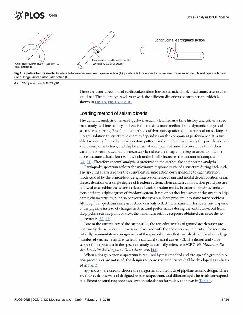
There are three directions of earthquake action: horizontal axial, horizontal transverse and lon-gitudinal. The failure types will vary with the different directions of earth action, which isshown in Fig. 1A, Fig. 1B, Fig. 1C.

Loading method of seismic loadsThe dynamic analysis of an earthquake is usually classified as a time history analysis or a spec-trum analysis. Time history analysis is the most accurate method in the dynamic analysis ofseismic engineering. Based on the methods of dynamic equations, it is a method for seeking anintegral solution to structural dynamics depending on the component performance. It is suit-able for solving forces that have a certain pattern, and can obtain accurately the particle acceler-ation, component stress, and displacement at each point of time. However, due to randomvariation of seismic action, it is necessary to reduce the integration step in order to obtain amore accurate calculation result, which undoubtedly increases the amount of computation[21–31]. Therefore spectral analysis is preferred in the earthquake engineering analysis.

Earthquake spectrum reflects the maximum response curve of a structure during each cycle.The spectral analysis solves the equivalent seismic action corresponding to each vibrationmode guided by the principle of designing response spectrum and modal decomposition usingthe acceleration of a single degree of freedom system. Then certain combination principles arefollowed to combine the seismic effects of each vibration mode, in order to obtain seismic ef-fects of the multiple degrees of freedom system. It not only takes into account the structural dy-namic characteristics, but also converts the dynamic force problem into static force problem.Although the spectrum analysis method can only reflect the maximum elastic seismic responseof the pipeline instead of changes in structural performance during the earthquake, but fromthe pipeline seismic point of view, the maximum seismic response obtained can meet the re-quirements [32–41].

Due to the uncertainty of the earthquake, the recorded results of ground acceleration arenot exactly the same even in the same place and with the same seismic intensity. The most sta-tistically representative average curve of the spectral curves that are calculated based on a largenumber of seismic records is called the standard spectral curve [42]. The design and valuescope of the spectrum in the spectrum analysis normally refers to ASCE 7–05:Minimum De-sign Loads for Buildings and Other Structures [43].

When a design response spectrum is required by this standard and site-specific ground mo-tion procedures are not used, the design response spectrum curve shall be developed as indicat-ed in Fig. 2.

SDS and SD1 are used to choose the categories and methods of pipeline seismic design. Thereare four cycle intervals of designed response spectrum, and different cycle intervals correspondto different spectral response acceleration calculation formulae, as shown in Table 1.

Fig 1. Pipeline failure mode. Pipeline failure under axial earthquake action (A), pipeline failure under transverse earthquake action (B) and pipeline failureunder longitudinal earthquake action (C).

doi:10.1371/journal.pone.0115299.g001



Stress analysis methodThe finite element is a commonly used method in pipe stress analysis. Different from softwaressuch as ANSYS, CAESAR II reflects pipe stress and displacement by calculating the pipelineunit endpoint, and the method is simpler to add constraints or load.

The analysis of long-distance pipeline stress in the earthquake region is generally dividedinto two modules: (1) static analysis and (2) dynamic analysis. Static analysis is the basis ofstress analysis. Its main purpose is to analyse the distribution of stress or displacement of thepipe in the absence of seismic conditions. Dynamic analysis is used to analyse the stress and

Fig 2. Design response spectrums.


Table 1. Spectral response acceleration calculation formulae.

Interval Computational formula

0�T�T0 Sa ¼ 23FaSsð0:4þ 0:6 Tp

T0Þ

T0�T�Ts Sa ¼ 23FaSs

Ts�T�TL Sa ¼ 2FvS13Tp

TL�T Sa ¼ 2FvS1TL3T2

p

Sa: Spectral acceleration, g (g is the local gravitational acceleration, with the unit of m/s2); SS: Spectral

acceleration for short cycles (damping factor is 5%); S1: Spectral acceleration with the cycle as 1s

(damping factor is 5%); Fa, Fv: Venue coefficient; Tp: Inherent cycle of a structure; T0: Cycle of response

spectral characteristics, T0 = 0.2SD1/SDS; Ts: Cycle of response spectrum characteristics Ts = SD1/SDS; TL:

Transitional period of long cycle; SDS: Design spectral response acceleration for short cycle (damping

factor is 5%); SD1: Design spectral acceleration with the cycle of 1s (damping factor is 5%).

doi:10.1371/journal.pone.0115299.t001



displacement of the pipeline under the earthquake situation. For pipelines in special terrains(such as those crossing earthquake zones, landslide areas and swamps), usually both modulesare needed in the analysis.

1. Static stress analysis. The main content of static analysis is to establish the correspondingmodel in accordance with the pipeline construction plans, and to determine the combinationtype of the working conditions based on pipeline loads, whereby the static analysisis performed.

Establishment of the pipeline system: the basic pipeline parameters (i.e., pipeline diameter,pipeline thickness, materials, etc.) and the environmental parameters (i.e., pipeline operatingtemperature and pressure) must be input into the operational interface.

Establishment of constraints: based on engineering practice, constraints must be simplifiedand then input into the operational interface.

Establishment of load cases: because the medium inside the pipeline and its environmentare different at different stages, the load cases must be established based on the different loadsfrom production to operation.

Exporting analysis results: the static stress analysis report is generated from thesoftware calculations.

2. Dynamic earthquake analysis. Depending on the load characteristics of the earthquakezone, dynamic analysis is adding seismic effects on the pipe to make it as close as possible tothe actual project. By calculating the various ground motion parameters, the calculated acceler-ation will be transformed into seismic effects and added onto the basic pipe model, enablingdynamic analysis of the pipeline to be performed.

Define the frequency spectrum: input the earthquake related coefficients and CAESAR IIcan generate the corresponding frequency spectrogram.

Spectrum loading: define the loading coefficients, direction, and the seismically affectedstart and end points of the pipeline.

Dynamic load condition combination: the loads are combined and loaded in thepipeline model.

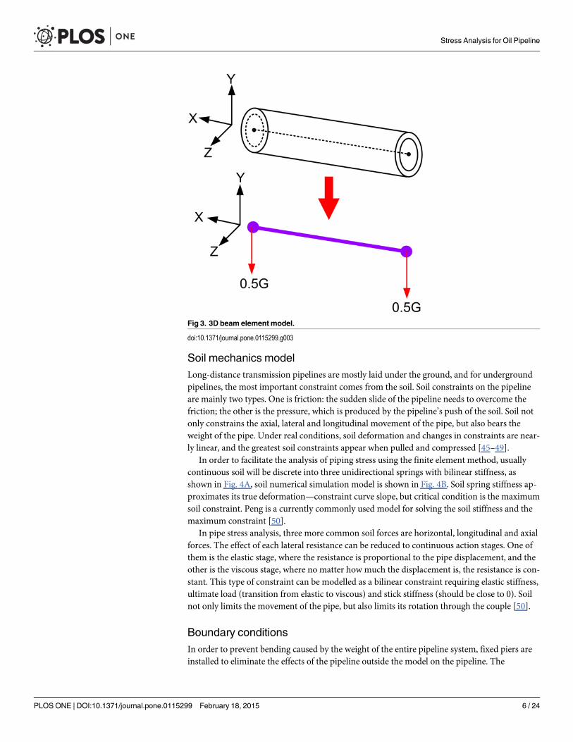
Pipeline mechanics modelPipe stress analysis is based on the finite element method, and the finite element models cangenerally be divided into the beam model and the shell model. As the pipeline itself is an axi-symmetric closed cylindrical shell, the shell model for analysis would be more accurate. How-ever, in order to save computer resources, usually 3D beam element model is adopted. This isbecause in an earthquake area, the length of the pipe is much larger than its diameter, and themajor consideration is the bending deformation rather than the deformation and stress withinthe pipe cross-section. Long-term engineering practice has also shown that for pipes withthe diameter no more than 100, using beam element model can meet the computationalaccuracy [17].

As shown in Fig. 3, the 3D beam element model’s simulation of the pipeline is a rigid ele-ment with six degrees of freedom. The mechanical behaviour of each unit (each pipe section) isdescribed with the endpoints, i.e., the objects of stress calculation are the two ends of a pipeunit, and the weight of the pipe is evenly distributed to both ends of the pipe unit [20, 44]. Themechanical hypothesis of the 3D beam unit is as follows:

1. The pipe is a pure bending deformation, which obeys Hooke’s law;

2. Ignore the effects of shear stress;

3. Constraint effects are on the centre line of the unit.



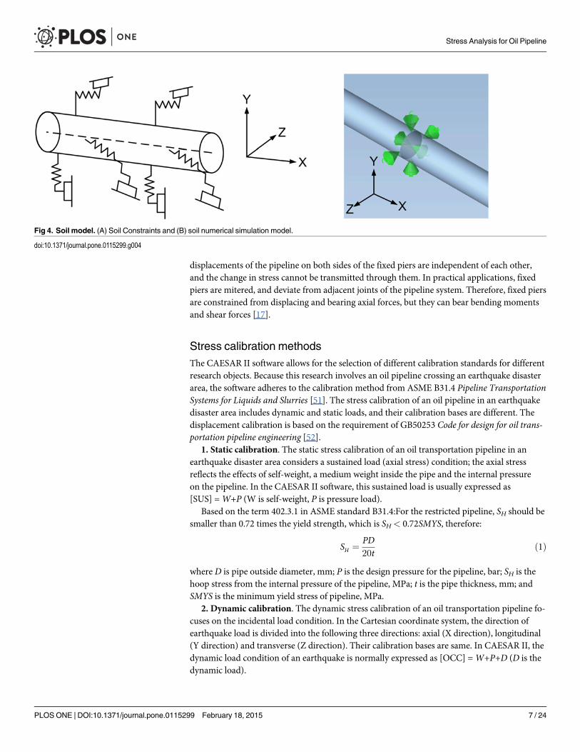
Soil mechanics modelLong-distance transmission pipelines are mostly laid under the ground, and for undergroundpipelines, the most important constraint comes from the soil. Soil constraints on the pipelineare mainly two types. One is friction: the sudden slide of the pipeline needs to overcome thefriction; the other is the pressure, which is produced by the pipeline’s push of the soil. Soil notonly constrains the axial, lateral and longitudinal movement of the pipe, but also bears theweight of the pipe. Under real conditions, soil deformation and changes in constraints are near-ly linear, and the greatest soil constraints appear when pulled and compressed [45–49].

In order to facilitate the analysis of piping stress using the finite element method, usuallycontinuous soil will be discrete into three unidirectional springs with bilinear stiffness, asshown in Fig. 4A, soil numerical simulation model is shown in Fig. 4B. Soil spring stiffness ap-proximates its true deformation—constraint curve slope, but critical condition is the maximumsoil constraint. Peng is a currently commonly used model for solving the soil stiffness and themaximum constraint [50].

In pipe stress analysis, three more common soil forces are horizontal, longitudinal and axialforces. The effect of each lateral resistance can be reduced to continuous action stages. One ofthem is the elastic stage, where the resistance is proportional to the pipe displacement, and theother is the viscous stage, where no matter how much the displacement is, the resistance is con-stant. This type of constraint can be modelled as a bilinear constraint requiring elastic stiffness,ultimate load (transition from elastic to viscous) and stick stiffness (should be close to 0). Soilnot only limits the movement of the pipe, but also limits its rotation through the couple [50].

Boundary conditionsIn order to prevent bending caused by the weight of the entire pipeline system, fixed piers areinstalled to eliminate the effects of the pipeline outside the model on the pipeline. The

Fig 3. 3D beam element model.




displacements of the pipeline on both sides of the fixed piers are independent of each other,and the change in stress cannot be transmitted through them. In practical applications, fixedpiers are mitered, and deviate from adjacent joints of the pipeline system. Therefore, fixed piersare constrained from displacing and bearing axial forces, but they can bear bending momentsand shear forces [17].

Stress calibration methodsThe CAESAR II software allows for the selection of different calibration standards for differentresearch objects. Because this research involves an oil pipeline crossing an earthquake disasterarea, the software adheres to the calibration method from ASME B31.4 Pipeline TransportationSystems for Liquids and Slurries [51]. The stress calibration of an oil pipeline in an earthquakedisaster area includes dynamic and static loads, and their calibration bases are different. Thedisplacement calibration is based on the requirement of GB50253 Code for design for oil trans-portation pipeline engineering [52].

1. Static calibration. The static stress calibration of an oil transportation pipeline in anearthquake disaster area considers a sustained load (axial stress) condition; the axial stressreflects the effects of self-weight, a medium weight inside the pipe and the internal pressureon the pipeline. In the CAESAR II software, this sustained load is usually expressed as[SUS] =W+P (W is self-weight, P is pressure load).

Based on the term 402.3.1 in ASME standard B31.4:For the restricted pipeline, SH should besmaller than 0.72 times the yield strength, which is SH< 0.72SMYS, therefore:

SH ¼ PD20t

ð1Þ

where D is pipe outside diameter, mm; P is the design pressure for the pipeline, bar; SH is thehoop stress from the internal pressure of the pipeline, MPa; t is the pipe thickness, mm; andSMYS is the minimum yield stress of pipeline, MPa.

2. Dynamic calibration. The dynamic stress calibration of an oil transportation pipeline fo-cuses on the incidental load condition. In the Cartesian coordinate system, the direction ofearthquake load is divided into the following three directions: axial (X direction), longitudinal(Y direction) and transverse (Z direction). Their calibration bases are same. In CAESAR II, thedynamic load condition of an earthquake is normally expressed as [OCC] =W+P+D (D is thedynamic load).

Fig 4. Soil model. (A) Soil Constraints and (B) soil numerical simulation model.




Based on the term 402.3.1 in ASME standard B31.4: The sum of the longitudinal stressesproduced by pressure, live and dead loads, and those produced by occasional loads, such aswind or earthquake, shall not exceed 80% of the specified minimum yield strength of the pipe,which is SL � 0.80SMYS, therefore:

SL ¼ EaðT2 � T1Þ � nSh ð2Þ

where SL is longitudinal stresses, MPa; SMYS is the minimum yield strength of the pipe, MPa;E is the modulus of elasticity of steel, MPa; Sh is the hoop stress from fluid pressure, MPa; T1 isthe temperature at time of installation, °C; T2 is the maximum or minimum operating tempera-ture, °C; α is the linear coefficient of thermal expansion, mm/mm°C; ν is Poisson’s ratio(ν = 0.30 for steel).

3. Displacement calibration. There is no accurate standard for the pipeline displacementcalibration. In section 5.6.2 of GB50253 Code for design for oil transportation pipeline engineer-ing, there is a general specification for the displacement condition of a steel pipeline: the maxi-mum displacement of a steel pipeline in the horizontal direction should not exceed 0.03 timesthe average diameter of the steel pipeline, which is

Dx � 0:03D ð3Þwhere Δx is the maximum displacement of the steel pipeline in the horizontal direction, m; andD is the average diameter of the steel pipeline, m.

Case Study

Project introductionBased on the design materials for the XX earthquake disaster location, X80 steel pipe is usedfor the oil pipeline, the installation temperature is 20°C, the running temperature is 80°C andthe operating pressure is 8 MPa. The ambient temperature of the pipeline is 20°C, the backfillsoil is saturated coarse sand and the seismic intensity level is 7, (a low probability earthquakefor limit-state design consideration). The basic seismic acceleration is 0.30 g, the elevation ofthe bottom slope at the west side of the pipeline is 361.66 m, the elevation of the middle slope is383.95 m and the elevation of the top slope is 408.33 m. The direction of the pipeline is shownas Fig. 5. The detailed parameters of the pipeline layout are shown in Table 2. The specific pipe-line, soil and earthquake parameters are shown in Tables 3–5.

The pipe is a spatial model, i.e., there are the length components in all three directions of X,Y, Z. The total length of the pipeline model is 780 m. fixed piers 1 and 2 are set at the start andend points, respectively, of the pipeline. There is 30 m of pipeline before the west side soil en-trance (guidance point B), and the entrance angle is 30°. The west horizontal section is 110 mand the inclined pipeline is 215 m. There is 30 m of pipeline after the east exit (guidancepoint I), and the exit angle is 30°. The east horizontal section is 105 m and the east inclinedpipeline is 290 m. The curvature radius of the bended pipeline is R = 10D, in which D is theoutside diameter [16].

Earthquake analysis and loadingBased on the earthquake related materials for the XX pipeline and the GB50011–2010 Code forseismic design of buildings, the ground’s characteristic period and the maximum value of thehorizontal seismic coefficient can be obtained. According to Formulas (4) and (5), the responseacceleration SS of the short period design spectrum of the damping coefficient is 4% (the U.S.nuclear pipeline design manual requires that the damping coefficient equals 4%) and the



response acceleration S1 of the design spectrum with a one second period is calculated. Basedon Tables 11.4–1 and 11.4–2, from ASCE 7–05, the site coefficients Fa and Fv are determined.After inputting the related earthquake frequency spectrum parameters into the frequency spec-trum analysis modules, the analysis chart will be generated by the software. The frequencyspectrum parameters of the XX pipeline are shown in Table 6.

SS ¼ 1:604amax=Fa ð4Þ

S1 ¼ 1:604T0:918g amax=Fv ð5Þ

where αmax is the maximum value of the horizontal earthquake affecting factor, 0.72 in thiscase; and Tg is the characteristic period of the ground.

After loading the spectrum to the pipeline model, the earthquake working conditions mustbe established. We analysed one static working condition and four dynamic working condi-tions. The dynamic condition comprises occasional load condition in each of the axial direction(X direction), the longitudinal direction (Y direction) and the transverse direction (Z direc-tion), as well as the occasional load condition with three directions combined with the stresschecking method identical to one-direction occasional load conditions. Of particular note isthat the combined occasional load condition is established through transforming into seismicaction the acceleration calculated based on the spectrum in three directions, and loading theseismic action on the pipeline by combining load conditions. The integrated seismic

Fig 5. Spatial layout of a pipeline in an earthquake disaster area.


Table 2. Special location parameters of pipelines.

Azimuth Pipe Segment Axial Deviation (°) Longitudinal Grade (°) Remarks

West Side AB 30 0 A is the pipe’s starting point, that is anchor block 1

BC 0 0 B is the guiding point for the west side pipe

CD 0–15 15 ——

DE 0–10 5 ——

EF 0–15 15 ——

FG 0–10 10 ——

East Side GH 0–15 15 ——

HI 0 0 I is the guiding point for the east side pipe

IJ 30 0 J is the pipe’s end point, which is anchor block 2




acceleration (force) is calculated following acceleration (force) synthesis theorem in the Carte-sian coordinate system. The working condition combinations are listed Table 7.

Results

Numerical Simulation resultAfter building the dynamic load and combining the working conditions, the CAESAR II soft-ware can produce the dynamic stress analysis report, which includes the details of the pipelinestress, displacement, constraints loading, etc. Because the pipeline start points, end points, westside guidance section and east side guidance section aim to reduce the influence from the pipe-line located outside the model, when performing the stress analysis, the displacement and stressof these four special locations can be neglected in the XX earthquake disaster section. Conse-quently, the pipeline is studied from 32 m-740 m (I.e., from point B to point I, and not includ-ing bends 1 and 8).

After gathering the maximum displacement and stress (Tables 8 and 9), in the comprehensiveseismic load condition, the maximum axial, longitudinal displacement and transverse displace-ment are generated at the bend in the pipeline on the top of the slope (bend 6). The followingconclusions can be drawn after calibrating the static stress, dynamic stress and displacement: themaximum stress ratio does not exceed calibrated stress, which meets the strength requirement;and the maximum transverse displacement does not exceed 0.03D = 12.2 mm, which meets thedisplacement requirement. Comparing the maximum axial displacement and the longitudinaldisplacement during seismic activity, the maximum transverse displacement is larger. Therefore,in actual projects, it is suggested to add the corresponding pipeline parts necessary to restrain thetransverse displacement of the pipeline.

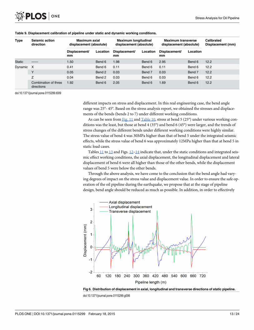
Figs. 6–9 shows the axial, longitudinal and transverse displacement distributions along thepipeline under static conditions and earthquake activity, respectively. The displacement duringearthquake activity is calculated using the SRSS (Square Root of the Sum of the Squares) meth-od [53–60] (This is one of the many types of modal combination method. This method as-sumes that events involved in data processing are completely independent of each other. Whenthe difference between natural vibration states of a structure or between the natural vibrationfrequencies is large, it can be approximately considered that the vibration of each mode is inde-pendent of each other, so that a better result can be obtained, but the symbol of the vibration

Table 3. Pipeline parameters.

Material Diameter (mm) Thickness (mm) Corrosion allowance (mm) Thickness of insulation layer (mm)

X80 406 7.1 1 60

Density of oil (kg�m-3) Installation temperature (°C) Operation temp (°C) Operation pressure (MPa) Minimum yield strength (MPa)

900 20 80 8 551.58


Table 4. Soil parameters.

Type Friction coefficient Density (kg�m-3) Temperature variation (°C)

Dried coarse sand 0.6 2600 60

Soil Friction Angle (°) Compaction coefficient Thermal expansion coefficient Yield Displacement Factor (L/L/°C)

30 5 11.214×10–6 0.015




model cannot be displayed.). All calculated values are positive, which indicates the pipeline’smaximum distance at a certain moment but does not show the movement direction; therefore,the static displacement situation has been presented separately. Fig. 10 displays the distributionof stress ratios along the pipeline under static conditions and earthquake activity. Based onFigs. 6–10, the following can be concluded:

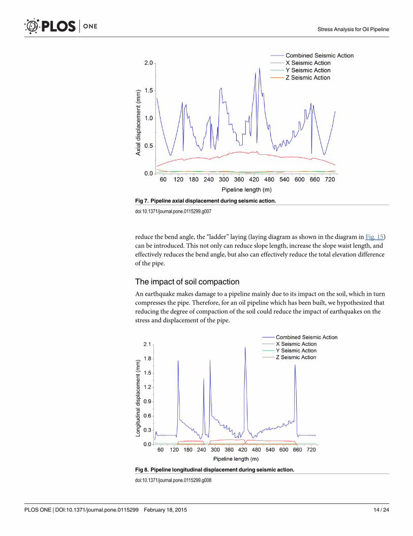
1. Compared to the transverse and longitudinal earthquake action, the axial (X direction)earthquake action causes greater changes to the axial, longitudinal and transverse displace-ments, which suggests the necessity to include axial earthquake action controls intothe design.

2. The pipeline stress distribution trends during earthquake activity and static conditions ex-hibit a high degree of unity; the stress value under dynamic earthquake activity is relativelygreater. For earthquake action in a single direction, the transverse earthquake activity effectis slightly larger than the effects of the earthquake activity in the other two directions

3. Under combined seismic activity, the displacement and stress of a pipeline are greater thanany one single direction seismic activity, indicating that the combined earthquake activitycauses the greatest damage to the pipeline.

4. The maximum displacement value and maximum stress are generated at the bent pipe onthe top of the slope and on the bottom of the west slope; the stress value at the bent pipechanges suddenly. Consequently, during oil pipeline operation, there is a stress concentra-tion at the bend location, which is the critical section of the oil pipeline in an earthquake di-saster area. The stress calibrations for the bent pipeline at the top and bottom of the slopemust be calculated. If the stress and displacement exceed the limits, a reinforcement mea-sure must be implemented.

5. Stress analysis usually occurs before the pipeline is put into production, and the objects ofthe analysis are new steel pipes. In actual engineering, there may be cracks on the pipe dueto construction and other reasons. Based on the analysis results, we can conclude that theearthquake will exacerbate cracks in the pipe in varying degrees. As the earthquake has sig-nificant impact on the lateral displacement of the pipeline, it means that the earthquake hasgreat impact on the extension of cracks along the axial direction of the pipeline. It is there-fore proposed that in oil pipeline defect detection in earthquake regions, attention should bepaid to issues such as crack repair.

Table 6. Spectrum Parameters.

Component significant coefficient Land coefficient SS S1 Modified response coefficient

Fa Fv

1.5 1.0 1.3 1.24 0.70 3.5


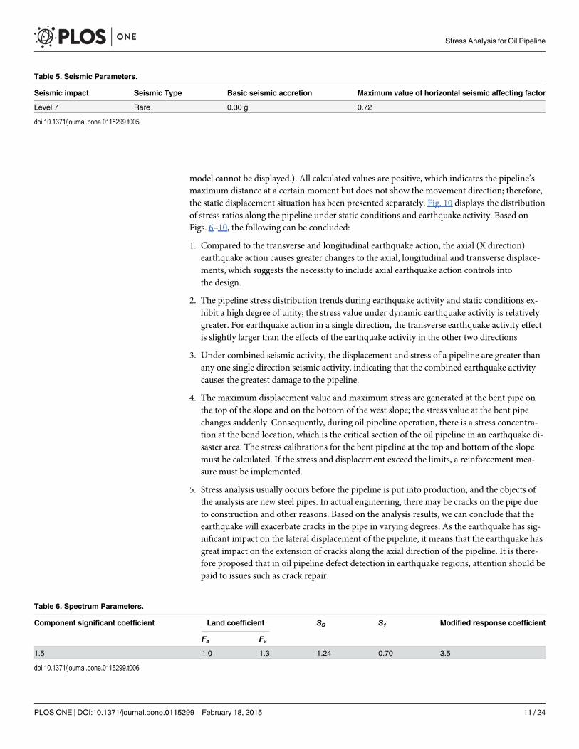
Table 5. Seismic Parameters.

Seismic impact Seismic Type Basic seismic accretion Maximum value of horizontal seismic affecting factor

Level 7 Rare 0.30 g 0.72




Experiment resultIn order to verify the correctness of the numerical simulation results and the reasonableness ofthe model, field experiments were conducted and the results were compared with numericalsimulation results. As the test system, which includes the work strain gauges, compensationstrain gages, strain gauges and computers installed on the multiple sections of the pipe, hadbeen installed before the pipeline was put into production, we selected earlier recorded resultsof stress and strain with the seismic intensity of 7. Because the pipeline was long, we only se-lected data at the section of critical stress (bends 2 to 7), and compared them with the numeri-cal simulation results. Relative error analysis (two decimal places) of the numerical simulationand field experimental data is calculated as follows:

Relative error ¼Numerical simulation data� Experimental dataExperimental data

� 100% ð6Þ

The main factors leading to the experimental measurement error were: wire resistance, temper-ature, sensitivity coefficient, and moisture of strain gauges. Since the annual rainfall in the areais relatively small, the environment relatively dry, and the impact of wire resistance, tempera-ture and the sensitivity coefficients on the measurement relatively small, they were negligible.Error analysis results showed that the range of the absolute value of the relative error of thestress test was 0.95%-3.09%, and the absolute value range of the relative error of the displace-ment was 0.51%-4.49%, within the acceptable range. This suggested that numerical simulationdata had a certain degree of credibility, and the model was relatively reasonable.

Discussions

The impact of the bend anglesOil transmission pipelines adopt the elastic laying method, that is, when the line directionchanges, the spatial direction of the pipe can be changed relying on the gravity and elasticbending, without on-site installation of cold simmer bends. Different bend angles have

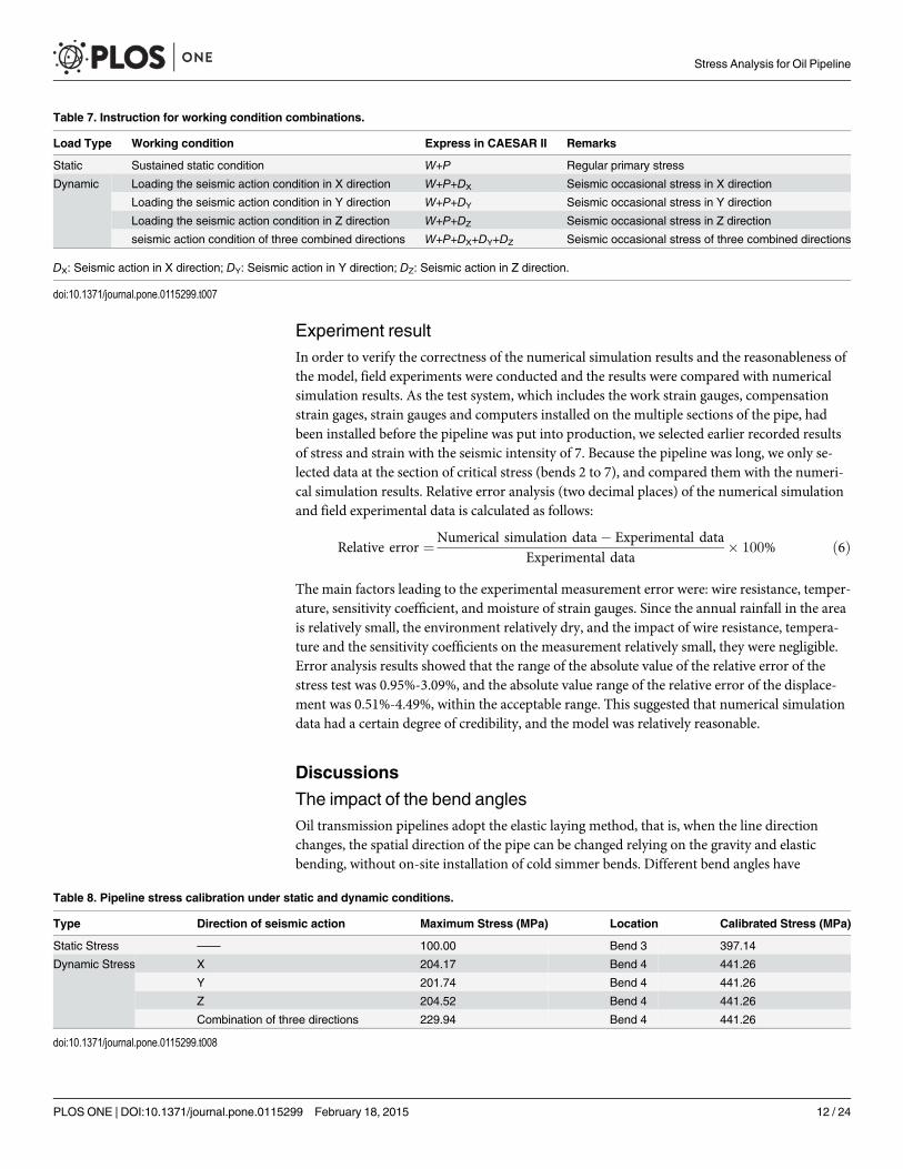
Table 7. Instruction for working condition combinations.

Load Type Working condition Express in CAESAR II Remarks

Static Sustained static condition W+P Regular primary stress

Dynamic Loading the seismic action condition in X direction W+P+DX Seismic occasional stress in X direction

Loading the seismic action condition in Y direction W+P+DY Seismic occasional stress in Y direction

Loading the seismic action condition in Z direction W+P+DZ Seismic occasional stress in Z direction

seismic action condition of three combined directions W+P+DX+DY+DZ Seismic occasional stress of three combined directions

DX: Seismic action in X direction; DY: Seismic action in Y direction; DZ: Seismic action in Z direction.


Table 8. Pipeline stress calibration under static and dynamic conditions.

Type Direction of seismic action Maximum Stress (MPa) Location Calibrated Stress (MPa)

Static Stress —— 100.00 Bend 3 397.14

Dynamic Stress X 204.17 Bend 4 441.26

Y 201.74 Bend 4 441.26

Z 204.52 Bend 4 441.26

Combination of three directions 229.94 Bend 4 441.26




different impacts on stress and displacement. In this real engineering case, the bend anglerange was 25°- 45°. Based on the stress analysis report, we obtained the stresses and displace-ments of the bends (bends 2 to 7) under different working conditions.

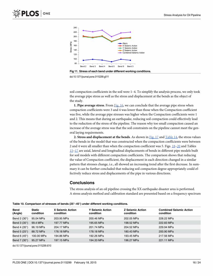
As can be seen from Fig. 11 and Table 10, stress at bend 5 (25°) under various working con-ditions was the least, but those at bend 4 (35°) and bend 6 (45°) were larger, and the trends ofstress changes of the different bends under different working conditions were highly similar.The stress value of bend 4 was 30MPa higher than that of bend 5 under the integrated seismiceffects, while the stress value of bend 6 was approximately 12MPa higher than that at bend 5 instatic load cases.

Tables 11 to 13 and Figs. 12–14 indicate that, under the static conditions and integrated seis-mic effect working conditions, the axial displacement, the longitudinal displacement and lateraldisplacement of bend 6 were all higher than those of the other bends, while the displacementvalues of bend 5 were below the other bends.

Through the above analysis, we have come to the conclusion that the bend angle had vary-ing degrees of impact on the stress value and displacement value. In order to ensure the safe op-eration of the oil pipeline during the earthquake, we propose that at the stage of pipelinedesign, bend angle should be reduced as much as possible. In addition, in order to effectively

Table 9. Displacement calibration of pipeline under static and dynamic working conditions.

Type Seismic actiondirection

Maximum axialdisplacement (absolute)

Maximum longitudinaldisplacement (absolute)

Maximum transversedisplacement (absolute)

CalibratedDisplacement (mm)

Displacement/mm

Location Displacement/mm

Location Displacement/mm

Location

Static —— 1.50 Bend 6 1.98 Bend 6 2.95 Bend 6 12.2

Dynamic X 0.41 Bend 6 0.11 Bend 6 0.11 Bend 6 12.2

Y 0.05 Bend 2 0.03 Bend 7 0.03 Bend 7 12.2

Z 0.04 Bend 2 0.03 Bend 6 0.03 Bend 6 12.2

Combination of threedirections

1.92 Bend 6 2.05 Bend 6 1.69 Bend 6 12.2


Fig 6. Distribution of displacement in axial, longitudinal and transverse directions of static pipeline.




reduce the bend angle, the “ladder” laying (laying diagram as shown in the diagram in Fig. 15)can be introduced. This not only can reduce slope length, increase the slope waist length, andeffectively reduces the bend angle, but also can effectively reduce the total elevation differenceof the pipe.

The impact of soil compactionAn earthquake makes damage to a pipeline mainly due to its impact on the soil, which in turncompresses the pipe. Therefore, for an oil pipeline which has been built, we hypothesized thatreducing the degree of compaction of the soil could reduce the impact of earthquakes on thestress and displacement of the pipe.

Fig 7. Pipeline axial displacement during seismic action.


Fig 8. Pipeline longitudinal displacement during seismic action.




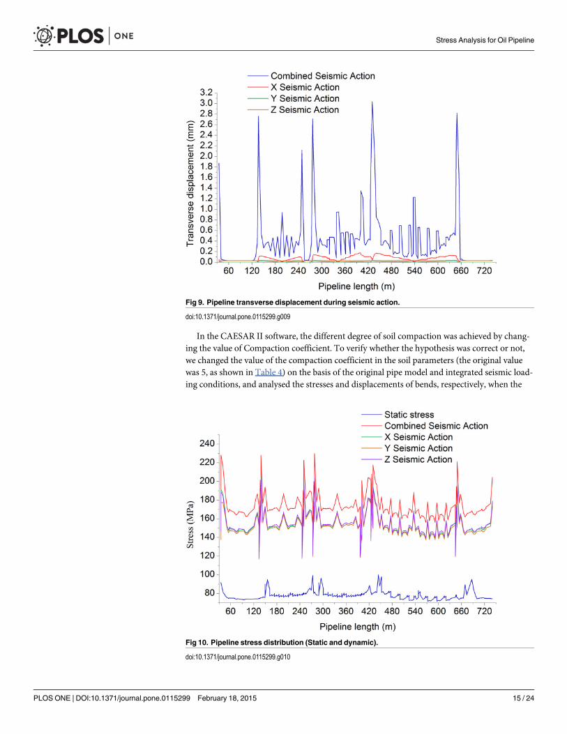
In the CAESAR II software, the different degree of soil compaction was achieved by chang-ing the value of Compaction coefficient. To verify whether the hypothesis was correct or not,we changed the value of the compaction coefficient in the soil parameters (the original valuewas 5, as shown in Table 4) on the basis of the original pipe model and integrated seismic load-ing conditions, and analysed the stresses and displacements of bends, respectively, when the

Fig 9. Pipeline transverse displacement during seismic action.


Fig 10. Pipeline stress distribution (Static and dynamic).




soil compaction coefficients in the soil were 1–4. To simplify the analysis process, we only tookthe average pipe stress as well as the stress and displacement at the bends as the object ofthe study.

1. Pipe average stress. From Fig. 16, we can conclude that the average pipe stress whencompaction coefficients were 3 and 4 was lower than those when the Compaction coefficientwas five, while the average pipe stresses was higher when the Compaction coefficients were 1and 2. This means that during an earthquake, reducing soil compaction could effectively leadto the reduction of the stress of the pipeline. The reason why too small compaction caused anincrease of the average stress was that the soil constraints on the pipeline cannot meet the gen-eral laying requirements.

2. Stress and displacement at the bends. As shown in Fig. 17 and Table 14, the stress valuesof the bends in the model that was constructed when the compaction coefficients were between2 and 4 were all smaller than when the compaction coefficient was 5. Figs. 18–20 and Tables15–17 are axial, lateral and longitudinal displacements of bends in different pipe models builtfor soil models with different compaction coefficients. The comparison shows that reducingthe value of Compaction coefficient, the displacement in each direction changed in a similarpattern that stresses change, i.e., all showed an increasing trend after the first decrease. In sum-mary it can be further concluded that reducing soil compaction degree appropriately could ef-fectively reduce stress and displacements of the pipe in various directions.

ConclusionsThe stress analysis of an oil pipeline crossing the XX earthquake disaster area is performed.A stress analysis method and calibration standard are presented based on a frequency spectrum

Fig 11. Stress of each bend under different working conditions.


Table 10. Comparison of stresses of bends (25°–45°) under different working conditions.

Bend(Angle)

Staticcondition

X Seismic Actioncondition

Y Seismic Actioncondition

Z Seismic Actioncondition

Combined Seismic Actioncondition

Bend 2 (30°) 95.04 MPa 203.95 MPa 200.46 MPa 202.05 MPa 228.22 MPa









method. The location of the critical section and maximum stress area can be pinpointed clearlythrough this stress analysis. The corresponding remediation measures should be implementedbased on the stress analysis.

Based on the limit-state design thinking for strength, the seismic activity with a smallerprobability but severe destructive effect is loaded on the pipeline. Analysis of the stress to theXX oil transportation pipeline confirms that the bent section of the pipeline is the critical sec-tion, particularly the bended pipe at the top and bottom of the slope. The maximum axial,transverse and longitudinal displacements are generated at the bend in the pipe at the top ofthe slope. The earthquake activity in the axial direction poses a greater influence on the axial,longitudinal and transverse displacements. The following recommendation is presented basedon the analysis: during the construction process in earthquake disaster areas, if the displace-ment will approach or exceed the allowable standard when the pipeline is in operation, then itis imperative to install the necessary pipe parts and shock absorbers to control the displacementof pipeline.

In addition, our discussion about the bend angle and degree of soil compaction as the de-pendent variables led to the conclusion that: (1) reducing the bend angle could reduce the stressand displacement of the underground pipe during an earthquake, and “Ladder” could beadopted for laying pipes; (2) appropriately reducing the degree of soil compaction could reducethe impact of the earthquake on the stress and displacement.

The proposed calibration standard, frequency analysis method and working condition load-ing for earthquake stress on a pipeline provides a safety reference for the design of an oil pipe-line crossing an earthquake disaster area. This also fills the technology gap for the stressanalysis of an oil transportation pipeline in seismic disaster locations.

Table 11. Comparison of axial displacements of bends (25°–45°) under different conditions.

Bend(Angle)

Staticcondition





Bend 2 (30°) 0.933 mm 0.273 mm 0.048 mm 0.043 mm 1.299 mm

Bend 3 (35°) 0.701 mm 0.264 mm 0.044 mm 0.036 mm 1.044 mm

Bend 4 (35°) 1.152 mm 0.314 mm 0.043 mm 0.043 mm 1.553 mm

Bend 5 (25°) 0.629 mm 0.383 mm 0.020 mm 0.039 mm 0.936 mm

Bend 6 (45°) 1.500 mm 0.410 mm 0.025 mm 0.035 mm 1.917 mm

Bend 7 (30°) 0.930 mm 0.260 mm 0.041 mm 0.044 mm 1.280 mm


Table 12. Comparison of longitudinal displacements of different bends (25°–45°) under different working conditions.

Bend(Angle)

Staticcondition





Bend 2 (30°) 1.678 mm 0.065 mm 0.029 mm 0.017 mm 1.767 mm

Bend 3 (35°) 1.304 mm 0.041 mm 0.027 mm 0.018 mm 1.391 mm

Bend 4 (35°) 1.676 mm 0.080 mm 0.027 mm 0.017 mm 1.775 mm

Bend 5 (25°) 0.048 mm 0.100 mm 0.027 mm 0.010 mm 0.138 mm

Bend 6 (45°) 1.977 mm 0.108 mm 0.023 mm 0.026 mm 2.048 mm

Bend 7 (30°) 1.598 mm 0.073 mm 0.030 mm 0.013 mm 1.686 mm




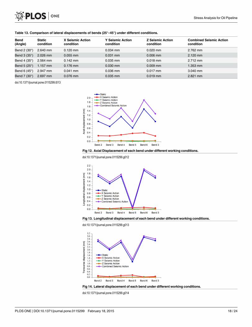
Table 13. Comparison of lateral displacements of bends (25°–45°) under different conditions.

Bend(Angle)

Staticcondition





Bend 2 (30°) 2.640 mm 0.120 mm 0.034 mm 0.020 mm 2.762 mm

Bend 3 (35°) 2.026 mm 0.055 mm 0.031 mm 0.006 mm 2.120 mm

Bend 4 (35°) 2.564 mm 0.142 mm 0.035 mm 0.018 mm 2.712 mm

Bend 5 (25°) 1.157 mm 0.176 mm 0.030 mm 0.009 mm 1.353 mm

Bend 6 (45°) 2.947 mm 0.041 mm 0.036 mm 0.017 mm 3.040 mm

Bend 7 (30°) 2.697 mm 0.076 mm 0.035 mm 0.019 mm 2.821 mm


Fig 12. Axial Displacement of each bend under different working conditions.


Fig 13. Longitudinal displacement of each bend under different working conditions.


Fig 14. Lateral displacement of each bend under different working conditions.




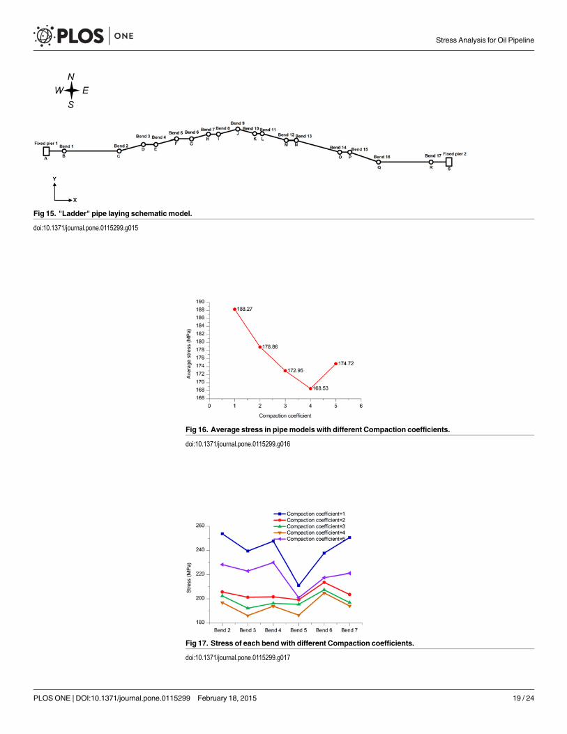
Fig 17. Stress of each bend with different Compaction coefficients.


Fig 15. "Ladder" pipe laying schematic model.


Fig 16. Average stress in pipemodels with different Compaction coefficients.




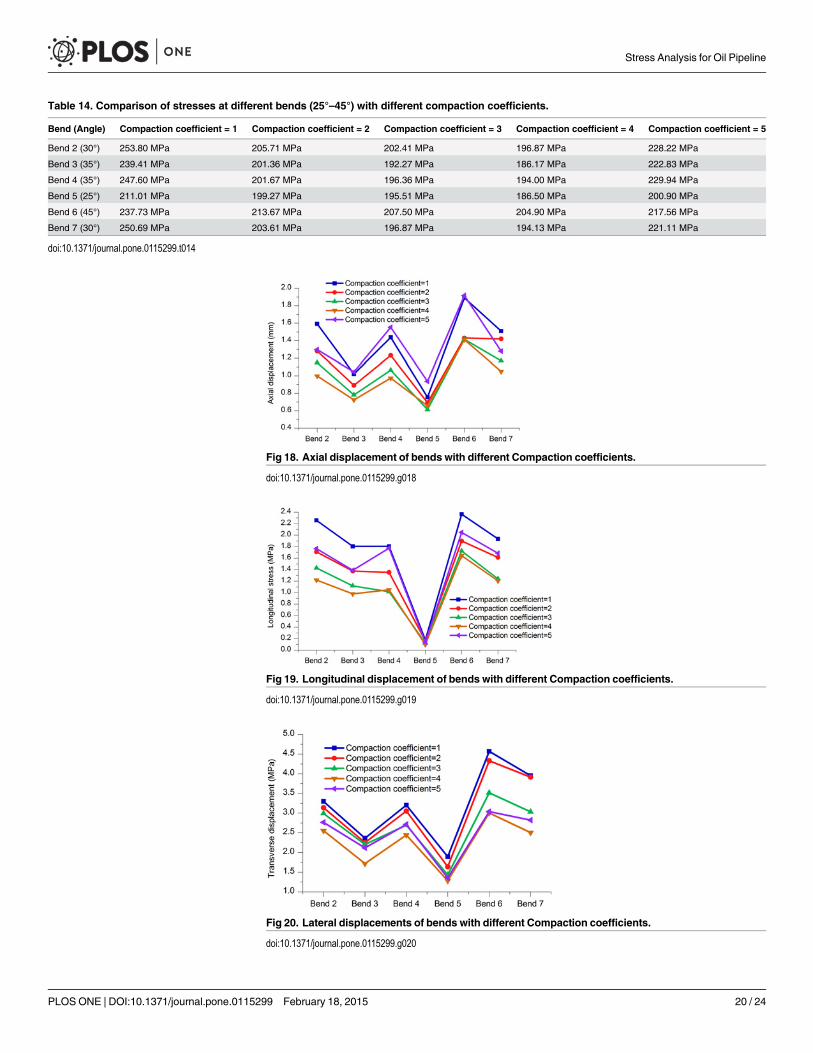
Fig 18. Axial displacement of bends with different Compaction coefficients.


Table 14. Comparison of stresses at different bends (25°–45°) with different compaction coefficients.

Bend (Angle) Compaction coefficient = 1 Compaction coefficient = 2 Compaction coefficient = 3 Compaction coefficient = 4 Compaction coefficient = 5








Fig 20. Lateral displacements of bends with different Compaction coefficients.


Fig 19. Longitudinal displacement of bends with different Compaction coefficients.




Author ContributionsConceived and designed the experiments: XNWHFL. Performed the experiments: HFL. Ana-lyzed the data: HFL SJW. Contributed reagents/materials/analysis tools: XNWHFL KHWBQ.Wrote the paper: HFL SJW.

References1. Metropolo PL, Brown AEP (2004) Natural gas pipeline accident consequence analysis. Process Safety

Progress 23(4): 307–310.

2. Hao JB, Liu JP, Zhang J, Jing HY, Han B, et al. (2009) Risk of earthquake hazard to long-distance oiland gas pipelines. Oil and Gas Storage and Transportation 28(11): 27–30.

3. Zhang HB, Feng QS, Zheng HL, Zhou LJ, Wu XY (2010) Earthquake risk evaluation method of oil andgas pipelines. Oil and Gas Storage and Transportation 29(1): 15–17.

4. Zeng J, Xu JC, Chen GH, Yuan JB (2007) Applicability of Risk Assessment Method for Urban BuriedGas Pipeline. Gas & Heat 5: 55–61. doi: 10.1016/j.ijscr.2014.10.038 PMID: 25603393

Table 15. Comparison of axial displacements of bends (25°–45°) with different Compaction coefficients.


Bend 2 (30°) 1.592 mm 1.281 mm 1.150 mm 0.999 mm 1.299 mm

Bend 3 (35°) 1.020 mm 0.890 mm 0.782 mm 0.725 mm 1.044 mm

Bend 4 (35°) 1.437 mm 1.233 mm 1.064 mm 0.973 mm 1.553 mm

Bend 5 (25°) 0.755 mm 0.693 mm 0.613 mm 0.657 mm 0.936 mm

Bend 6 (45°) 1.890 mm 1.430 mm 1.416 mm 1.412 mm 1.917 mm

Bend 7 (30°) 1.510 mm 1.420 mm 1.170 mm 1.050 mm 1.280 mm


Table 17. Comparison of lateral displacements of bends (25°–45°) with different Compaction coefficients.


Bend 2 (30°) 3.295 mm 3.139 mm 2.989 mm 2.554 mm 2.762 mm

Bend 3 (35°) 2.362 mm 2.250 mm 2.205 mm 1.718 mm 2.120 mm

Bend 4 (35°) 3.205 mm 3.052 mm 2.693 mm 2.443 mm 2.712 mm

Bend 5 (25°) 1.890 mm 1.635 mm 1.430 mm 1.283 mm 1.353 mm

Bend 6 (45°) 4.569 mm 4.330 mm 3.513 mm 3.006 mm 3.040 mm

Bend 7 (30°) 3.955 mm 3.913 mm 3.032 mm 2.503 mm 2.821 mm


Table 16. Comparison of longitudinal displacements of bends (25°- 45°) with different Compaction coefficients.


Bend 2 (30°) 2.259 mm 1.709 mm 1.430 mm 1.221 mm 1.767 mm

Bend 3 (35°) 1.805 mm 1.376 mm 1.119 mm 0.979 mm 1.391 mm

Bend 4 (35°) 1.806 mm 1.353 mm 1.017 mm 1.050 mm 1.775 mm

Bend 5 (25°) 0.176 mm 0.160 mm 0.123 mm 0.097 mm 0.138 mm

Bend 6 (45°) 2.366 mm 1.899 mm 1.725 mm 1.643 mm 2.048 mm

Bend 7 (30°) 1.935 mm 1.613 mm 1.240 mm 1.205 mm 1.686 mm




http://dx.doi.org/10.1016/j.ijscr.2014.10.038

http://www.ncbi.nlm.nih.gov/pubmed/25603393

5. Zhang P, Duan YH (1998) An idea and method of the long distance transmission pipeline risk tech-nique. Natural Gas Industry 18(5): 72–76.

6. China National Petroleum Corporation (2009) GB 50470–2008 Seismic technical code for oil and gastransmission pipeline engineering. Beijing: China Planning Press.

7. Watkins RK, Anderson LR (1999) Structural mechanics of buried pipes. Boca Raton: CRC press.

8. Yu GQ, Lv ZH (2008). Load calculation and analysis of heating pipeline based on elastic center method.Gas and Heat 28(12): 20–24.

9. Rajani BB, Robertson PK, Morgenstern NR (1995). Simplified design methods for pipelines subject totransverse and longitudinal soil movements. Canadian Geotechnical Journal 32(2): 309–323.

10. Zhang DH, Lv YM (1999). Calculation of thermal stress intensity factor for semi-elliptical surface cracksof thin pipeline. Oil and Gas Storage and Transportation 18(1): 13–17.

11. Wu XN, Xian Y, Huang K, Hu ML, Shang BJ (2012) The stress analysis of tunnel gas pipeline under op-erating situation. Oil and Gas Storage and Transportation 31(12): 927–930.

12. Huang K, Wu SJ, Lu HF, Xian Y, Su QW (2012) Stress analysis of the pipeline laid along the slope. Nat-ural Gas and Oil 30(4): 1–4.

13. Wu XN, Shu HW, Zan LF, Jiang X, Hu DH, et al. (2013) Stress analysis of a gas pipeline through shieldtunnels under pressure test conditions. Natural Gas Industry 33(3): 73–77.

14. Wu XN, Lu HF, Wu SJ, Huang K, Chen X, et al. (2014) Analysis of suspended pipeline stress sensitivity.Applied Mechanics and Materials 501–504: 2331–2334.

15. Huang K, Lu HF, Shen KR, Shu HW, Wang YJ (2013) Study on Buttresses Distance of Gas Pipelines inthe DeviatedWell Based on Stress Analysis Method. Advance Journal of Food Science and Technolo-gy 5(9): 1249–1254.

16. Wu XN, Lu HF, Huang K, Tang XY, Wu SJ, et al. (2014) Stress analysis of gas pipelines at seismicbelts based on the spectrum analysis. Natural Gas Industry 34(5): 152–157.

17. Jiang X, Wang TY, Sun L, Wu X (2013) Stress analysis of unburied gas pipelines laid in high slopes.Natural Gas and Oil 31(6): 26–30.

18. Chen LQ, Wu SJ, Lu HF, Huang K, Lv YT, et al. (2014) Stress analysis of buried gas pipeline traversingsliding mass. Open Civil Engineering Journal 8: 239–243.

19. Wu XG, Zhou Q, Lu HF (2014) Stress analysis of CAESAR II—based buried oil pipelines. PipelineTechnique and Equipment 2: 16–18.

20. George M (1998). Pipe stress analysis theory guide. Beijing: COADE Inc China Technical Service andTraning Center.

21. Lilhanand K, TsengWS (1988) Development and application of realistic earthquake time histories com-patible with multiple-damping design spectra. Development 3: 7–8.

22. Gupta AK, Chu SL (1976) Design of reinforced concrete structures subjected to three components ofearthquake. Nuclear Engineering and Design 36(1): 96–101.

23. Scanlan RH, Sachs K (1974) Earthquake time histories and response spectra. Journal of the Engineer-ing Mechanics Division 100(4): 635–655.

24. Kim S, D’Amore E (1999) Push-over analysis procedure in earthquake engineering. Earthquake Spec-tra 15(3): 417–434.

25. Singh MP, Ghafory-Ashtiany M (1986) Modal time history analysis of non-classically damped structuresfor seismic motions. Earthquake Engineering & Structural Dynamics 14(1): 133–146. doi: 10.1098/rsta.2014.0086 PMID: 25583865

26. Ji C, Wald DJ, Helmberger DV (2002) Source description of the 1999 Hector Mine, California, earth-quake, part I: Wavelet domain inversion theory and resolution analysis. Bulletin of the SeismologicalSociety of America 92(4): 1192–1207.

27. Cheng M, Popplewell N (1994). Neural network for earthquake selection in structural time history analy-sis. Earthquake Engineering & Structural Dynamics 23(3): 303–319. doi: 10.1098/rsta.2014.0086PMID: 25583865

28. Naeim F, Lew M (1995) On the use of design spectrum compatible time histories. Earthquake Spectra11(1): 111–127.

29. Spanos PD, Vargas Loli LM (1985) A statistical approach to generation of design spectrumcompatible earthquake time histories. International Journal of Soil Dynamics and Earthquake Engineer-ing 4(1): 2–8.

30. WangW (2012) The comparative analysis of response spectrummethod and time analysis method inanti-seismic design of tall building. Master dissertation, South China University of Technology,Guangzhou.



http://dx.doi.org/10.1098/rsta.2014.0086





31. Li JL, Zhao J, Li FH, He YL, Kang CC (2011) Analysis of time—history analysis method on the seismicdesign. Earthquake Research in Sichuan 4: 25–28.

32. Brune JN (1970) Tectonic stress and the spectra of seismic shear waves from earthquakes. Journal ofGeophysical Research 75(26): 4997–5009.

33. Rautian TG, Khalturin VI (1978) The use of the coda for determination of the earthquake source spec-trum. Bulletin of the Seismological Society of America 68(4): 923–948.

34. Sabetta F, Pugliese A (1996) Estimation of response spectra and simulation of nonstationary earth-quake ground motions. Bulletin of the Seismological Society of America 86(2): 337–352.

35. Boore DM (1983) Stochastic simulation of high-frequency ground motions based on seismologicalmodels of the radiated spectra. Bulletin of the Seismological Society of America 73(6A): 1865–1894.

36. Wyss M (1973) Towards a physical understanding of the earthquake frequency distribution. Geophys-ical Journal International 31(4): 341–359.

37. Hanks TC (1979) b values andω−γ seismic source models: Implications for tectonic stress variationsalong active crustal fault zones and the estimation of high—frequency strong ground motion. Journal ofGeophysical Research: Solid Earth (1978–2012) 84(B5): 2235–2242.

38. Aki K (1969) Analysis of the seismic coda of local earthquakes as scattered waves. Journal of Geo-physical Research 74(2): 615–631.

39. Frankel A (1991) High—frequency spectral falloff of earthquakes, fractal dimension of complex rupture,b value, and the scaling of strength on faults. Journal of Geophysical Research: Solid Earth(1978–2012) 96(B4): 6291–6302.

40. Atkinson GM, Silva W (1997) An empirical study of earthquake source spectra for California earth-quakes. Bulletin of the Seismological Society of America 87(1): 97–113.

41. Aki K (1984) Asperities, barriers, characteristic earthquakes and strong motion prediction. Journal ofGeophysical Research: Solid Earth (1978–2012) 89(B7): 5867–5872.

42. Ministry of Housing and Urban-Rural Development of the People’s Republic of China (2009) GB50011–2010 Code for seismic design of buildings. Beijing: China Architecture and Building Press. doi:10.1016/j.vetimm.2014.02.004 PMID: 24629764

43. ASCE (2005) ASCE 7–05 Minimum Design Loads for Buildings and Other Structures. Reston: Ameri-can Society of Civil Engineers Press. doi: 10.1016/j.febslet.2014.10.035 PMID: 25447518

44. Sreejith B, Jayaraj K, Ganesan N, Padmanabhan C, Chellapandi P, Selvaraj P (2004) Finite elementanalysis of fluid—structure interaction in pipeline systems. Nuclear Engineering and Design 227(3):313–322.

45. Pyke R (1979) Nonlinear soil models for irregular cyclic loadings. Journal of the Geotechnical Engineer-ing Division 105(6): 715–725.

46. Gysi M (2001) Compaction of a Eutric Cambisol under heavy wheel traffic in Switzerland: Field dataand a critical state soil mechanics model approach. Soil and Tillage Research 61(3): 133–142.

47. Hettiaratchi DRP (1987) A critical state soil mechanics model for agricultural soils. Soil Use and Man-agement 3(3): 94–105.

48. Roscoe KH (1970). The influence of strains in soil mechanics. Geotechnique 20(2): 129–170.

49. Ting JM, Corkum BT, Kauffman CR, Greco C (1989) Discrete numerical model for soil mechanics. Jour-nal of Geotechnical Engineering 115(3): 379–398.

50. Peng LC (1978) Stress analysis methods for underground pipelines. Pipe Line Industry, 47(5): 65–74.

51. ASME (2013) ASME B31.4–2012 Pipeline Transportation Systems for Liquids and Slurries.New York: American Society of Mechanical Engineers Press, 2013. doi: 10.1115/1.4028414 PMID:25554734

52. CNPC (2007) GB 50253–2006 Code for design of oil transportation pipeline engineering. Beijing:China Planning Press.

53. Wilson EL, Der Kiureghian A, Bayo EP (1981) A replacement for the SRSSmethod in seismic analysis.Earthquake Engineering & Structural Dynamics 9(2): 187–192. doi: 10.1098/rsta.2014.0086 PMID:25583865

54. Sinha R, Igusa T (1995) CQC and SRSSmethods for non-classically damped structures. EarthquakeEngineering & Structural Dynamics 24(4):615–619. doi: 10.1098/rsta.2014.0086 PMID: 25583865

55. Menun C, Der Kiureghian A (1998) A replacement for the 30%, 40%, and SRSS rules for multicompo-nent seismic analysis. Earthquake Spectra 14(1): 153–163.

56. Lopez OA, Chopra AK, Hernandez JJ (2000) Critical response of structures to multicomponent earth-quake excitation. Earthquake Engineering & Structural Dynamics 29(12): 1759–1778. doi: 10.1098/rsta.2014.0086 PMID: 25583865



http://dx.doi.org/10.1016/j.vetimm.2014.02.004


http://dx.doi.org/10.1016/j.febslet.2014.10.035


http://dx.doi.org/10.1115/1.4028414









57. SmebyW, Der Kiureghian A (1985) Modal combination rules for multicomponent earthquake excitation.Earthquake Engineering & Structural Dynamics 13(1): 1–12. doi: 10.1098/rsta.2014.0086 PMID:25583865

58. Wilson EL, Suharwardy I, Habibullah A (1995) A clarification of the orthogonal effects in a three-dimensional seismic analysis. Earthquake Spectra 11(4): 659–666.

59. Penzien J (1997) Evaluation of building separation distance required to prevent pounding during strongearthquakes. Earthquake Engineering & Structural Dynamics 26(8): 849–858. doi: 10.1098/rsta.2014.0086 PMID: 25583865

60. Singh MP (1980) Seismic response by SRSS for no proportional damping. Journal of the EngineeringMechanics Division 106(6): 1405–1419.








frequency spectrum method-based stress analysis for oil pipelines

Documents