MASTER’S THESIS

2010:003 PB

MASTER’S THESIS

Universitetstryckeriet, Luleå

2010:003 PB

Shaojie Kang

Friction and Elasto-Plastic deformation in Asperity Collision

M.Sc. in Engineering mechanics CONTINUATION COURSES

Luleå University of Technology Department of Applied Physics and Mechanical Engineering

Division of Machine Elements

MASTER’S THESIS

Universitetstryckeriet, Luleå

2010:003 PB

Shaojie Kang

Friction and Elasto-Plastic deformation in Asperity Collision

M.Sc. in Engineering mechanics CONTINUATION COURSES

Luleå University of Technology Department of Applied Physics and Mechanical Engineering

Division of Machine Elements

Master Thesis

Friction and Elasto-plastic Deformation in Asperity Collision

Shaojie Kang

MASTER OF SCIENCE PROGRAMME

Division of Machine Element

Abstract The collision of cylindrical asperities is studied in this thesis. Numerical results are first compared and validated with classical Hertzian theory. Effects of the substrate material under the mating surface are considered in the simulation. Materials of top and bottom surfaces are given different properties. Elasto-plastic deformation and friction are determined along the process of collision. Strain hardening is included in the elasto-plastic deformation. Effects of interferences change and friction coefficient increase on deformation and friction are studied. Deformed shapes of each asperity are given after collision. In the end, a preliminary wear curve is created.

Nomenclature Interference Friction coefficient

1R Radius for top asperity

2R Radius for bottom asperity 'R Effective radius

1 Poisson ratio for top asperity

2 Poisson ratio for bottom asperity

1E Module of elasticity for top asperity

2E Module of elasticity for bottom asperity 'E Effective module of elasticity

nF Load per unit length

a Semi contact length P Contact pressure

2J Second invariant of the stress deviation A parameter

1 First principle stress

2 Second principle stress

3 Third principle stress

y Yield stress

eff Effective strain

ep Effective plastic strain

Q Total volume of wear debris produced W Total normal load H Hardness K Dimensionless constant L Sliding distance

Contents Chapter 1 Introduction..................................................................................................... 2 1.1 Boundary lubrication.................................................................................................. 4 1.2 Asperity collision ......................................................................................................... 5 1.3 Effects of lubricants .................................................................................................... 5 1.4 Objectives..................................................................................................................... 8 Chapter 2 Modeling process and material property setting ......................................... 9 2.1 Geometry of simulation model................................................................................... 9 2.2 Model settings............................................................................................................ 11 Chapter 3 Verificationof simulation results ................................................................. 13 3.1 Comparison between numerical and analytical results......................................... 13 Chapter 4 Plastic deformation and effects of friction components ............................ 16 4.1 Theory background of elasto-plastic deformation................................................. 17 Chapter 5 Results of elasto-plastic deformation and friction after collsion ............. 20 5.1 Elasto-plastic deformation ....................................................................................... 20 5.2 Friction....................................................................................................................... 28 5.3 Normal load ............................................................................................................... 31 Chapter 6 Preliminary wear model............................................................................... 33 6.1 Wear mechanisms ..................................................................................................... 33 6.2 Wear rate ................................................................................................................... 34 6.3 Preliminary wear curve ............................................................................................ 35 Conclusion ....................................................................................................................... 38 Future work ..................................................................................................................... 39 Acknowledgement ........................................................................................................... 40 Reference ......................................................................................................................... 41

1

Chapter 1

Introduction Tribology is the science and technology of interacting surfaces in relative motion. It incorporates various scientific and technological disciplines such as surface chemistry, fluid mechanics, materials, contact mechanics, electromagnetics, and lubrication systems. The study of tribology is commonly applied in bearing design but extends into almost all other aspects of modern technology, even to such unlikely areas as hair conditioners and cosmetics such as lipstick, powders and lip gloss. Any product where one material slides or rubs over another is affected by complex tribological interactions, lubricated cases as hip implants and other artificial prosthesis are widely used; for some cases if the conventional lubricants can not be used as in high temperature sliding wear, the formation of oxide layer have been observed to protect against wear. Tribology also plays an important role in manufacturing. In metal-forming operations, friction increases tool wear and the energy required to form a work piece. This results in increased costs due to more frequent tool replacement, loss of tolerance as tool dimensions shift, and greater forces are required to shape a piece. A layer of lubricant which eliminates surface contact virtually eliminates tool wear and decreases needed energy. Tribology is customarily divided into three branches: friction, lubrication, and wear. Friction is encountered whenever there is relative motion between contacting surfaces, and it always opposes the motion. As no mechanically prepared surfaces are perfectly smooth, when the surfaces are first brought into contact under light load, they touch only along the asperities (real area of contact). The early theories attributed friction to the interlocking of asperities; however, it is now understood that the phenomenon is far more complicated. Lubrication can greatly decrease friction and wear. When clean surfaces are brought into contact, their coefficient of friction decreases drastically if even a single molecular layer of a foreign substance (for example, an oxide) is introduced between the surfaces. For thicker lubricant films, the coefficient of friction can be quite small and no longer dependent on the properties of the surfaces but only on the bulk properties of the lubricant. Most common lubricants are liquids and gases, but solids such as molybdenum disulfide or graphite may be used. Wear is the progressive loss of substance of one body because of rubbing by another body. There are many different types of wear, including sliding wear, abrasive wear, corrosion, and surface fatigue. In sliding or rolling contacts different regimes of lubrication may exist, specified by Boundary Lubrication (BL), Mixed Lubrication (ML) and (Elasto) Hydrodynamic lubrication (EHL). In boundary lubrication the load is mainly carried by mechanical contact, this is for example the case at low velocity when the hydrodynamic pressure build up is negligible. In the BL regime the lubricant’s main function is to reduce friction and wear between the contacting surfaces. Mixed lubrication is in the region between the BL and HL regimes. The load is partly transmitted by hydrodynamic pressure, with the rest being transmitted by mechanical contact. Hence, friction levels will be between boundary and hydrodynamic lubrication. In (Elasto-) hydrodynamic lubrication, lubricant

2

film is formed between the mating surfaces in relative sliding or rolling motion because of the wedge-shaped macro-geometry. So the friction is greatly reduced and there is no mechanical contact.

Figure 1.1. Stribeck curve for different lubrication regimes The Stribeck curve is used to represent different lubrication regimes; on the y-axis is the friction coefficient, and is the film thickness parameter, which is usually defined as

2/122

21

min

)( RqRq

h

(1.1)

minh is film thickness. and are RMS surface roughness parameters, which describe the roughness height of the two surfaces. If surface roughness value can be smaller, then the boundaries between different lubrication regimes can be moved to the left.

1Rq 2Rq

Surface roughness is a very important parameter in the field of tribology. The real surface is not that smooth if a micro scale picture was taken, the real surface will look like in Fig.1.2.

3

1

Boundary Mixed Lubrication

Full film LubricationLubrication

3

Figure 1.2. Surface roughness

Each peak in Fig.1.2 is called an asperity. The purpose of this thesis is to simulate the collision between different asperities in the mating surface when there is a relative motion. First of all, two terms must be distinguished; they are nominal contact area and real contact area. If the load is applied on the top surface and brought into contact with the bottom surface, the load will be carried by the peaks of high asperities. Some of the low area in the valleys may not be in contact, so contact area is not the same as the nominal area which was used to calculate the pressure achieved by normal force divide nominal contact area. The real contact area is less than the nominal contact area, how much of the real contact area here is decided by normal load, surface roughness value, hardness, and elastic module etc.

1.1 Boundary lubrication As mentioned above, boundary lubrication is the lubrication regime where hydrodynamic action is negligible. The contact load is carried by asperities on both surfaces. High peak pressures and temperatures occur at the asperity summits when the surfaces slide relative to each other. The lubricant has an important role even if the lubricant cannot provide any hydrodynamic lift, but the lubricant can act with the surfaces to form a thin protective layer. Under more severe conditions, EP-additives have a similar behavior where for example sulphide films are formed instead of oxide films. If the protective layer is not strong enough, it may be ruptured and the bare surfaces may come into contact resulting in severe adhesive wear. So it can be said that, with all the three lubrication regimes, boundary lubrication is the most severe and dangerous regime because of the high level of friction and wear. If we can predict the friction and wear in boundary lubrication, then the life of the machine components may be greatly increased. Even though boundary lubrication is very common, only a few and highly simplified BL models can be found. These models are normally empirical and are only valid within a very limited parameter range.

4

1.2 Asperity collision The new surface is relatively rough. When two surfaces are sliding in relative motion, peaks of some high asperities will be sheared off; some asperities will be flattened down. This process is called running-in. Running-in is a severe wear mode because of the material loss. There will be more surfaces coming into contact after running in, the contact pressure will be greatly reduced; another phenomenon is that asperities whose initial high peaks were worn off will be harder due to strain hardening of the new surface. Reduced pressure and hardened new surface will cause a decrease in wear, so after running in wear will be in a mild state.

Figure 1.3. Modeling of asperity collision unit:[ m ] In boundary lubrication, the load is mainly carried by asperities, so it is necessary to model the collision behavior of asperities. If some parameters as contact pressure and friction force can be achieved from asperity collision, risks can be predicted. This will offer a possibility for engineers to reduce wear and prolong the lifetime of machine components. 1.3 Effects of lubricants In dry contact, the loads are all carried by metallic contact of asperities. Metallic contact of asperities can be greatly reduced when there is lubricant film between the mating surfaces. Parameters as the thickness of lubricant film, additives, viscosity of lubricant, operating temperature are very important in boundary lubrication.

5

Figure 1.4. Different reaction phenomenon in boundary lubrication

Figure 1.4 shows different reaction phenomena in boundary lubrication. The interactions occurs between additives and bare metal surface. There will be some bonds formed between molecules of additives and molecules on metal surface. The bonds in physisorption and chemisorption are weaker than metallic bonds in the bulk material. Anti-wear (AW) and Extreme pressure (EP) are two different types of chemical reactions. Both AW and EP additives can form a protective layer by chemical reaction with the metal surface. AW additives are used in the case of high temperature, and EP additives also called as anti-seizure or anti-scuffing additives are used in the case of high temperature and high load. In order to let the readers to get a more clear sense about additives, the mechanism of EP lubrication is introduced. If there is a high load applied leading the machine components to severe contacts between asperities, oxide layers will be removed at first, then bare metal surfaces come in contact with high reactivity and adhesion; in this situation, EP additives will rapidly forms sulphides, phosphides or phosphates, thus adhesion can be decreased and scuffing is avoided. Since this is just a fundamental research in the field of boundary lubrication, dry contacts or mechanical contacts are studied using the finite element method. Some researchers have already presented a lot of results in this field; their works are beneficial to this thesis. Greenwood and Williamson [1] established a framework for the asperity-contact based models of two contacting surfaces; but they did not include friction which can significantly affect the behavior of the asperity contacts. Zhang et al. [2] have presented a research on the effects of friction on the contact and deformation behavior in sliding asperity contacts; in their paper, the contact pressure and sub-surface stresses are calculated for a range of the normal approach and friction coefficient. But they did not include the strain hardening phenomenon in their simulation, which in reality will significantly affect the contact.

6

Tabor [3] in 1959 introduced the idea of junction grow, which is depending on a constant von Mises stress will be at the yield stress point. In his paper, he studied the effects of tangential load, he pointed out that when surfaces are first placed together under a normal load, plastic deformation occurs and the real contact area is proportional to the load and independent of the size of the bodies. Unfortunately Tabor did not give the exact solution for the stress field in the contact region and his model was suitable for high preload which can cause the elastic-plastic deformation. Many of researchers did their research based on Tabor’s work, Brizmer et al. [4] developed Tabor’s work, they proved the empirical relation between the junction growth and the normal preload with their numerical simulation results, and the effects of combined normal and tangential load on the evolution of contact area are investigated. The model they used was a deformable sphere in contact with a rigid flat under combined normal and tangential loading, the lack of this model is that it did not consider the deformation or the stress development in the bulk material. Jeng and Peng [5] also studied the junction growth of single asperity contact using almost the same model as the model given by Brizmer et al., but include the stress development in the bulk material. They studied the effects of the adsorbed layer on plastic deformation, the conclusion was that adsorbed layer has a significant effect on plastic deformation on small interference, but has no effects when the interference increases to a value of 35 o

A . But from the view of tribological contact, two asperities contact should be considered, not an asperity with a rigid flat surface. In this thesis, two dimensional asperity-asperity collision have been modeled in Comsol Multiphysics; The method is that the top asperity will move from left to right while at the same time the bottom asperity will stand still, thus depending on different interferences, the collision between two asperities will cause a serious level of contact pressures and friction forces. First of all numerical simulation results are compared with analytical solution within elastic deformation; then the effects of different interferences and friction coefficients are studied with elasto-plastic deformation, results as contact pressure and friction force are achieved. Moreover the plastic deformation zone and residual stress after contact are found. The results show that, for the same normal load, the friction reduces the contact pressure and increases the contact area. In the end, a simple wear model is created.

7

1.4 Objectives The goals of this thesis is to

Establish a first micro model for sliding contact surface-a collision model

Determine the deformations, stress distribution and friction force of colliding asperities

Find out the limits of damage for collision between asperities and the influence of

asperity interference and contact friction

Create a preliminary wear model

8

Chapter 2 Modeling process and material property setting The shapes of asperities are irregular in reality and there will be different shapes of each single asperity on the mating surfaces. Since this is a basic research into the field of asperity collision, the model to start with is a cylindrical shaped asperity in order to ease the modeling process. Compared with the model of one flat surface on half cylinder, this model is more close to the reality, because both of the surfaces are rough in reality. The author believes that this simplified model will offer some insights to the simulation with a model of irregular shaped asperities.

2.1 Geometry of simulation model To simulate asperity-asperity contact, Comsol Multiphysics has been used. First of all, a model of two half-cylinder contact has been created because less number of elements and simple geometry can reduce the calculating time. Figure 2.1 shows mesh of the model and simulation result for elastic deformation. The idea of this simulation is to move the top asperity from left to right while the bottom asperity is fixed on the bottom boundary. Simulation result was compared with Hertizian theory, which did not return a good comparison result.

Figure 2.1. Preliminary model of asperity collision. Left figure shows mesh of the

model and right figure shows the maximum von Mises stress The simulation result of this model is not well fit with Hertzian contact theory. Moreover it is not realistic, because when there is a large plastic deformation, the collision of asperities will affect the substrate material under the mating surfaces. So another more complicated model which has more boundaries and more meshes was developed.

9

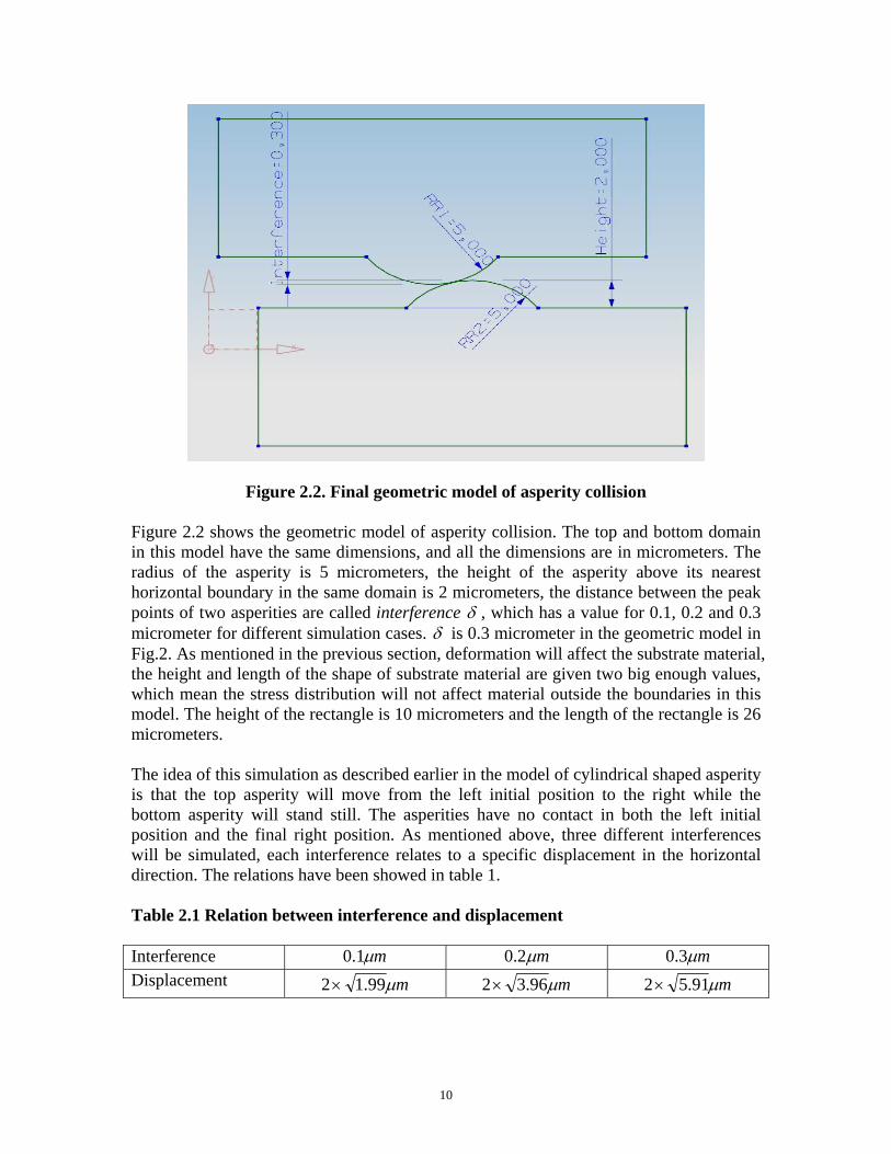
Figure 2.2. Final geometric model of asperity collision

Figure 2.2 shows the geometric model of asperity collision. The top and bottom domain in this model have the same dimensions, and all the dimensions are in micrometers. The radius of the asperity is 5 micrometers, the height of the asperity above its nearest horizontal boundary in the same domain is 2 micrometers, the distance between the peak points of two asperities are called interference , which has a value for 0.1, 0.2 and 0.3 micrometer for different simulation cases. is 0.3 micrometer in the geometric model in Fig.2. As mentioned in the previous section, deformation will affect the substrate material, the height and length of the shape of substrate material are given two big enough values, which mean the stress distribution will not affect material outside the boundaries in this model. The height of the rectangle is 10 micrometers and the length of the rectangle is 26 micrometers. The idea of this simulation as described earlier in the model of cylindrical shaped asperity is that the top asperity will move from the left initial position to the right while the bottom asperity will stand still. The asperities have no contact in both the left initial position and the final right position. As mentioned above, three different interferences will be simulated, each interference relates to a specific displacement in the horizontal direction. The relations have been showed in table 1. Table 2.1 Relation between interference and displacement

mInterference 1.0 m 2.0 m 3.0 Displacement m99.12 m96.32 m91.52

10

2.2 Model settings The plane strain module is used in Comsol since this is a two dimensional problem. For a contact problem, the contact pair has to be made between the contact boundaries; in this simulation, the top domain was considered as a stiff material and the bottom domain was considered as a soft material, so the boundaries in the top asperity were set as the master boundary and the boundaries in the bottom asperity were set as the slave boundary. Isotropic and elasto-plastic material modules were selected for elastic deformation and elastic-plastic deformation respectively.

Figure 2.3. Boundary conditions Boundary conditions Boundaries in red color in the top domain are free to move in the x direction but constrained in the y direction; Boundaries in green color in the bottom domain have been totally fixed in both x and y direction. Another boundary condition like that all the three boundaries of red color and two vertical boundaries of green color were released in y direction have also been applied to compare with the initial boundary conditions, the result shows that there is just 1% difference of von Mises stress. Material properties Stiffness difference is desired in order to let one asperity has a less plastic deformation and the other has more plastic deformation. Isotropic hardening mechanism has been used here for plastic deformation; this choice will be explained in Chapter 4. All the material data have been listed in table 2. Table 2.2 Properties of Material Young’s

module Yield stress Hardening

module Poisson ratio

Top asperity 210 GPa 1000 MPa 4500 MPa 0.3 Bottom asperity 160 GPa 600 MPa 4000 MPa 0.3

11

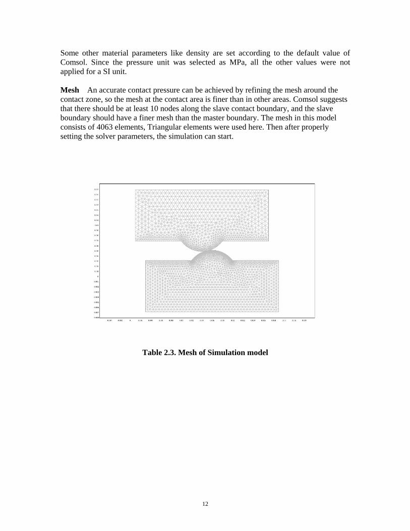
Some other material parameters like density are set according to the default value of Comsol. Since the pressure unit was selected as MPa, all the other values were not applied for a SI unit. Mesh An accurate contact pressure can be achieved by refining the mesh around the contact zone, so the mesh at the contact area is finer than in other areas. Comsol suggests that there should be at least 10 nodes along the slave contact boundary, and the slave boundary should have a finer mesh than the master boundary. The mesh in this model consists of 4063 elements, Triangular elements were used here. Then after properly setting the solver parameters, the simulation can start.

Table 2.3. Mesh of Simulation model

12

Chapter 3

Verification of simulation results Numerical simulation results are always based on either experimental result or analytical theory. Since the behavior of asperity collision is in the micro scale, it is very hard to compare with experimental results here. Fortunately Hertzian contact theory can be used to compare with the numerical results if linear elastic deformation is assumed.

3.1 Comparison between numerical and analytical results To prove that this simulation has been made in a correct way, the simulation result of elastic deformation has been compared with the analytical result calculated from Hertzian theory. For elastic deformation, isotropic material module which has the property of linear elastic deformation was used in order to avoid plastic deformation. Elastically deformed asperities will be returned to the initial shape after collision.

Figure 3.1. Contact stress when two asperities are symmetrical Figure 4 was taken from the position which had the biggest contact stress and pressure, von Mises criterion was used to present the stress level. The interference for this validation model is 0.1 micrometer. The unit in figure 4 is in millimeter. For line contact, the Hertz theory is given as below.

1

21

11'

RRR (1)

13

1

2

22

1

21 1()1(

2'

EEE

(2)

'

'8

E

RFa n

(3)

))(1(' 2xEF

P n

1R

2R'

'2 aR (4)

Where: Radius for top asperity

Radius for bottom asperity R Effective radius

1 Poisson ratio for top asperity

2 Poisson ratio for bottom asperity

Module of elasticity for top asperity 1E

Module of elasticity for bottom asperity 2E 'E Effective module of elasticity Load per unit length nF

a Contact length P Contact pressure

Figure 3.2. Comparison between analytical solution (dashed red) and numerical results (solid blue).

The solid blue curve and the dashed red curve are numerical and analytical result respectively. The reason to the slight deviation at the bottom might be because the mesh

14

of the model is not fine enough. The other reason maybe because the boundary conditions are not one hundred percent the same as in reality, as mentioned in the section of boundary conditions, results will differ 1% with different boundary conditions. The answer from Comsol Multiphysics Corporation is that maybe the deviation with negative contact pressure is a numerical error. Without this “numerical error”, Figure 3.2 shows a good agreement between numerical results and analytical solution.

15

Chapter 4 Plastic deformation and effects of friction components From mechanics point of view, when tensile load is applied to a specimen of ductile metal, extension of the specimen will occur and specimen will return to its initial shape when tensile load is removed, this deformation process is called elastic deformation. Each increment of load is related to corresponding increment in extension. But when the effect of load makes the tensile stress exceed yield stress, the specimen will not return to the initial shape after removing load, this deformation process is called plastic deformation.

Figure 4.1. Stress and strain relation

Elasto-plastic material was used in this simulation, which means the deformation will undergo an elastic deformation process when the stress is less than yield stress, but afterwards the mixed deformation of elastic and plastic will appear when the continually increasing stress exceeds yielding point. The shape of plastically deformed asperity will be permanently changed after contact. Figure 4.1 shows the stress and strain relation from the test of tensile load, x axis is effective strain and y axis is effective stress. y in the

figure is yield stress, when effective stress below it, the deformation is in elastic region, when effective stress above it, plastic flow starts. If the effective strain is exceeding the fracture point, the material can be sheared off. Such a phenomenon occurs in the running-in process.

Friction is undesirable in contacts such as between a camshaft and follower, because in most of the cases friction results in higher fuel or power consumption, and also because friction energy is transformed into heat which may cause machine elements to overheat.

16

Frictional heating may reduce the hardness of steel elements through metallurgical transformation, effective lubrication may fail or lubricant life decrease, machine parts may jam because of thermal expansion. In the field of tribology, friction is mainly divided into ploughing and adhesion. This can be explained with combination of the collision model in this thesis. The adhesive friction is modeled by a friction coefficient while the ploughing friction is modeled by the elastic-plastic deformation. There are totally 12 cases that have been simulated; they are 3 interferences cases and 4 friction coefficient cases in each interference case. But just some of the representative results will be showed to explain the collision process.

4.1 Theory background of elasto-plastic deformation If the stress exceeds the yield strength, the material will undergo plastic deformation. This critical stress can be tensile or compressive. Von Mises criteria [6] is commonly used to determine whether a material has yielded.

Von Mises criteria: This criterion is based on the Tresca criterion but takes into account the assumption that hydrostatic stresses do not contribute to material failure. Von Mises solves for an effective stress under uniaxial loading, subtracting out hydrostatic stresses, and claims that all effective stresses greater than that which causes material failure in uniaxial loading will result in plastic deformation.

In solid mechanics, von Mises criteria is usually defined as

0 22 JJf (4.1)

Where is a parameter and is the second invariant of the stress deviation, which is in the form of

2J

232

231

2212 6

1 J

1

(4.2)

Where , 2 and 3 are the first, second and third principal stresses respectively. The

yield stress can also be defined as follow:

2

322

312

212

1 y (4.3)

Von Mises criteria are used in the simulations of this thesis.

17

Work hardening: Work hardening is the strengthening of a material by plastic deformation. As the material becomes increasingly saturated with new dislocations, more dislocations are prevented from nucleating (a resistance to dislocation-formation develops). This resistance to dislocation-formation manifests itself as a resistance to plastic deformation; hence, the observed strengthening.

In metallic crystals, irreversible deformation is usually carried out on a microscopic scale by defects called dislocations, which are created by fluctuations in local stress fields within the material culminating in a lattice rearrangement as the dislocations propagate through the lattice. At normal temperatures the dislocations are not annihilated by annealing. Instead, the dislocations accumulate, interact with one another, and serve as pinning points or obstacles that significantly impede their motion. This leads to an increase in the yield strength of the material and a subsequent decrease in ductility.

For hardening materials, the yield surface will evolve in space in one of three ways. The first form of yield surface evolution is called isotropic hardening. For isotropic hardening, the yield surface grows in size while the center remains at a fixed point in stress space. The second form of surface evolution is called kinematic hardening. For kinematic hardening, the center of the yield surface translates in stress space, while the size remains fixed. The third type of surface evolution is called mixed hardening where both isotropic and kinematic hardening characteristics are evident. For mixed hardening, the orientation of the yield surface may also change as well. Although isotropic hardening is the most common form of yield surface evolution assumed in finite element models for metal forming simulation, it is not necessarily the most accurate. The mixed hardening model is most likely the most accurate of the three models.

Figure 4.3. Isotropic (left) and kinematic (right) hardening Circle represents the yield surface

18

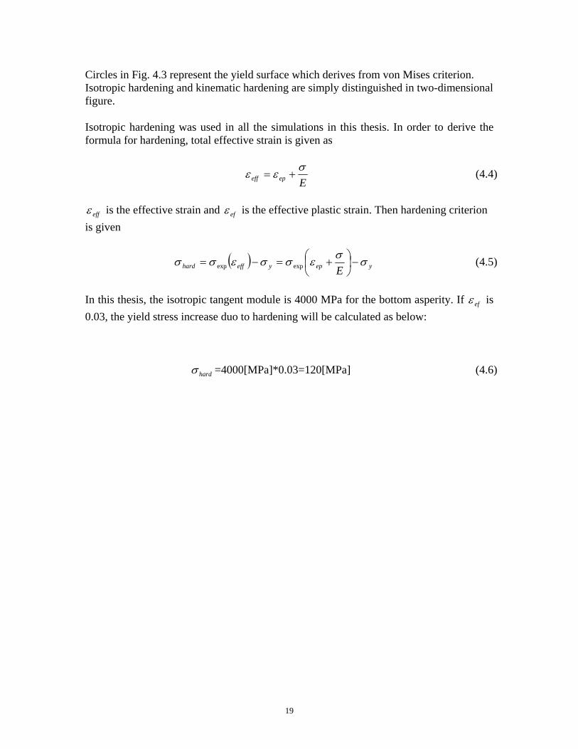
Circles in Fig. 4.3 represent the yield surface which derives from von Mises criterion. Isotropic hardening and kinematic hardening are simply distinguished in two-dimensional figure.

Isotropic hardening was used in all the simulations in this thesis. In order to derive the formula for hardening, total effective strain is given as

(4.4)

Eepeff

eff is the effective strain and ef is the effective plastic strain. Then hardening criterion

is given

yepyeffhard E

expexp

ef

(4.5)

In this thesis, the isotropic tangent module is 4000 MPa for the bottom asperity. If is

0.03, the yield stress increase duo to hardening will be calculated as below: hard =4000[MPa]*0.03=120[MPa] (4.6)

19

Chapter 5

Results of elasto-plastic deformation and friction after collision In this chapter, the development of the deformation will be given for interference 0.1 micrometers without friction coefficient and with friction coefficient 0.3 and interference 0.3 micrometers without friction coefficient and with friction coefficient 0.3.

5.1 Elasto-plastic deformation Eight sub graphs at different time steps will be given to show the collision process. Stress distribution can be clearly seen from each sub graph. The maximum von Mises stress in color scale is 1000 MPa which is the yield stress for top asperity. Material of top asperity is assumed to be protected, so it is harder than the bottom material and it is interesting to show a more accurate plastic deformation in top asperity. A color scale list is given in Table 5.1 to improve readability. Table 5.1 Color scale of von Mises stress Color Blue Green Yellow Orange Light red Deep red Stress [MPa] 0-400 400-600 600-700 700-800 800-900 900-1000 First of all, four different collision cases will be established with each case taking one complete page. Then the analysis of each case will be given after showing the collision process.

20

Figure 5.1. Collision process of 1.0 micrometer with 0

21

Figure 5.2. Collision process of micrometer with 3.01.0

22

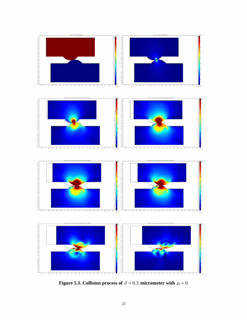
Figure 5.3. Collision process of micrometer with 03.0

23

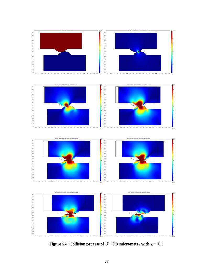
Figure 5.4. Collision process of micrometer with 3.03.0

24

Figure 5.1 shows the development of von Mises stress for micrometer with 1.00 . Maximum von Mises stress value was set to 1000 MPa in the color scale, so the

areas which exceed this value will be represented in the same deep red color. The stress development is not that regular as in elastic deformation because the plastically deformed shape will affect the lateral contact behavior.

micrometer with Figure 5.2 shows the development of the von Mises stress for 1.03.0 . Compared with the stress development in Fig. 5.1, there are not much

significant changes. The reason maybe because when the interference is not big enough, the effects of the friction coefficient on deformation and stress will not be significant.

0micrometer withFigure 5.3 shows the stress development for 3.0 ; Compared to the Figs. 5.1 and 5.2 above, the result will show that the increase of plastic deformation is very significant when the interference is increased. Compared to Fig. 5.3, the plastic deformation increase is still not significant in Fig. 5.4 when the interferences are the same but friction coefficient was increased from 0 to 3.0 . So the result can be given as interference changes contributed more on plastic deformation than friction coefficient changes.

25

0,1.0 m 31.0 .0, m

0,3.0 m 3.0,3.0 m

Figure 5.5. Deformed shapes of asperities after collision

When the plastic deformation is large, such as in Figs. 5.3 and 5.4, the asperity with permanently deformed shape will be clearly seen after the collision. The colors without blue left in the asperities means that there is some residual stress after the whole collision process. The residual stress is also larger with a bigger and value. Some materials will even be sheared off during this process, which is called running-in in the early chapter. Unfortunately it is still not possible to get rid of the removed material in Comsol, but when the strain of the material is larger than 0.3, this part of material was assumed to be sheared off. There will be more surface coming into contact because of plastically deformed asperity and removal of material, the pressure and stress level are not that high, thus high risk can be avoided. The asymmetric of the stress field in Fig. 5.5 is because the plastically deformed asperity will affect the lateral contact behavior which will give a different result compared to the stress distribution in elastically deformed asperity. Strain hardening might be another contribution to the asymmetric stress distribution.

26

Figure 5.6. Plastic deformation areas for top (upper) and bottom (down) asperity

Since the shape of asperities will be permanently changed when there is a plastic deformation, it is very interest to know how much of the areas are plastically deformed after the contact. Figure 5.6 shows the areas which are plastically deformed after contact for top and bottom asperity respectively. The bottom asperity has a bigger plastic deformation area than the top asperity because the yield stress for bottom asperity is lower than the top asperity. From both the top and bottom figure, it can be seen that the deformation change

27

is not significant with interference 0.1 micrometer even if there is a friction coefficient increase. It can be seen that when there is a friction coefficient increase, plastic deformation areas are not significantly changed, but after some value, especially with large interference, the friction coefficient increase will cause a clearly plastic deformation increase because more contacting surface can make the friction take more responsible for plastic deformation. This phenomenon will be explained in detail in next section.

5.2 Friction Bowden and Tabor in 1942 gave the definition of friction, which is defined as “Interfacial friction is caused by the ploughing of asperities in the mating surface and adhesion forces between the interacting asperity summits”. In this simulation, variation of different adhesive friction coefficients were presented, and variations of different ploughing frictions were presented. Comparison of both components showed that adhesion plays an important role in the overall friction. Definitions of ploughing and adhesion are given as below: Ploughing: If the hardness of sliding surfaces differs by>20% the roughness summits of the harder face penetrate the softer surface. During sliding motion this leads to the so-called ploughing of hard asperities into the softer mating surface. Hard particles, metal debris or dust particles from the environment may also contribute to this deformation. Adhesion: When two very smoothly-finished and cleaned surfaces are pressed together, they may stick together through atomic or inter-molecular forces. A distinction should be made between cohesive forces, which occur between identical mating materials, and adhesive forces, which occur between dissimilar mating materials. In this thesis, the surface traction force achieved form boundaries on the top asperity is called friction which is combined by ploughing and adhesion as normal sense; the force obtained from the boundaries between the top and bottom asperities is called adhesion. Ploughing will be related to interference and adhesion will be related to the applied friction coefficient on boundaries between top and bottom asperity.

28

Figure 5.7. Friction (left) and adhesion (right) for different interferences The total friction (left) and adhesion (right) are given in Fig. 5.7. When the friction coefficient applied on the boundaries between top and bottom asperities is zero, then there is no adhesion and the friction is purely formed by ploughing component. So there are four curves in each of the left graphs and three curves in each of the right graphs. It can be seen from all graphs that when the friction coefficient has been increased, the maximum friction and adhesion value will be moved from left to right. This is also duo to the plastic deformation increase.

29

Table 5.2 Maximum and average friction m =0 =0.1 =0.2 =0.3

Maximum value[N/mm]

0.153

0.327

0.535

0.772

0.1

Average value[N/mm]

0.0571

0.193

0.348

0.506

Maximum value[N/mm]

0.355

0.643

0.924

1.28

0.2

Average value[N/mm]

0.169

0.361

0.575

0.908

Maximum value[N/mm]

0.592

0.963

1.26

1.85

0.3

Average value[N/mm]

0.292

0.604

0.820

1.31

All the maximum and average frictions are calculated and listed in Table 5.2; the average friction is more meaningful because it represents the energy for one complete collision process. The trend of friction increase is also given in the figure below.

Figure 5.8. Maximum friction forces versus adhesive friction coefficient, =0.1 m ,

0.2 m , 0.3 m

30

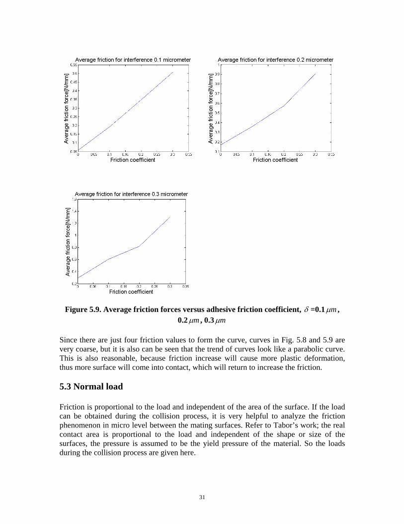
mFigure 5.9. Average friction forces versus adhesive friction coefficient, =0.1 , 0.2 m m , 0.3

Since there are just four friction values to form the curve, curves in Fig. 5.8 and 5.9 are very coarse, but it is also can be seen that the trend of curves look like a parabolic curve. This is also reasonable, because friction increase will cause more plastic deformation, thus more surface will come into contact, which will return to increase the friction. 5.3 Normal load Friction is proportional to the load and independent of the area of the surface. If the load can be obtained during the collision process, it is very helpful to analyze the friction phenomenon in micro level between the mating surfaces. Refer to Tabor’s work; the real contact area is proportional to the load and independent of the shape or size of the surfaces, the pressure is assumed to be the yield pressure of the material. So the loads during the collision process are given here.

31

In Fig. 5.10 below, vertical load applied on the top asperity is obtained from the integral of the contact pressure on the bottom asperity.

Figure 5.10. Normal load without (left) and with =0.3 (right) There is no significant change with normal load when friction coefficient changes, so the combination of load curve in the same interference is not to be given here. But compared with the two red curves in both graphs, it can be seen the maximum values are both around 4 N/mm. The cases with same friction coefficient and different interferences are given in Fig. 5.11. The difference is clearly enough to see when there is an interference increase, it can be said that interference change has a great effect on normal load. The maximum load is achieved at time step 0.5 when the top and bottom domain are symmetric in all four cases. When the collision process is finished, the load should be returned back to zero. The reason for nonzero load in the end in Fig. 5.11 is that the displacement is the same as in the elastic deformation. Because the shape of asperities are plastically deformed in this case, the displacement of the top asperity after the center line of the bottom asperity should be bigger than the displacement of top asperity before the centerline of the bottom asperity; then the two asperity can be totally separated. Since time is limited and the development of the load is interested here, not all the completely separated contact cases are done for the loads. But in all the average friction cases, the asperities in the end are completely separated.

32

Chapter 6 Preliminary wear model Wear [7] is defined as “the progressive loss of substance from the operating surface of a body occurring as a result of relative motion at the surface”. The loss of substance is what the engineers try to avoid in industry because of its enormous economic importance. Wear is very harmful to the machine performance because it increases clearances between the components, downgrading the precision of the machine and resulting in vibrations. In materials science, wear is the erosion of material from a solid surface by the action of another surface. It is related to surface interactions and more specifically the removal of material from a surface as a result of mechanical action. The need for mechanical action, in the form of contact due to relative motion, is an important distinction between mechanical wear and other processes with similar outcomes. 6.1 Wear mechanisms There are two main wear mechanisms which are two-body wear mechanism and three-body mechanism. Wear mechanisms that take place at the interface between two contacting bodies are defined as two-body wear mechanisms. Three-body wear mechanisms are classified as free solid particles between the surfaces which contribute to the wear process. Three body wear is a particular form of two-body wear. There are four fundamental classifications of two-body wear mechanisms, which are adhesive wear, abrasive wear, corrosive wear and surface fatigue. Two main wear mechanisms as adhesive wear and abrasive wear will be introduced in detail in the next section. Adhesive wear occurs when strong adhesive bonding between interacting asperities causes micro-welding, it is classified as formation and breaking of interfacial adhesive bonds. In a continuous movement, junctions shear off whereby material may transfer from one surface to the mating surface. Transfer can be either temporary or permanent. Temporary adhesion gives rise to free wear particles. Adhesive wear is generally so serious that it stops the machine. The surface becomes badly damaged and very high levels of friction and heat develop. Adhesive wear is commonly referred to as sliding wear. There are some methods which can decrease adhesive wear:

Combinations of non-metals or a non-metal against a metal Carburising or nitriding High hardness of both surfaces Strong oxide film Lubricant, liquid or solid Thin layer with low shear strength

33

Abrasive wear occurs when a hard rough surface slides across a softer surface. ASTM (American Society for Testing and Materials) define it as the loss of material due to hard particles or hard asperities that are forced against and move along a solid surface.

Abrasive wear is commonly classified according to the type of contact and the contact environment. The type of contact determines the mode of abrasive wear. The two modes of abrasive wear are known as two-body and three-body abrasive wear. Two-body wear occurs when the grits, or hard particles, are rigidly mounted or adhere to a surface, when they remove the material from the surface. The common analogy is that of material being removed with sand paper. Three-body wear occurs when the particles are not constrained, and are free to roll and slide down a surface. The contact environment determines whether the wear is classified as open or closed. An open contact environment occurs when the surfaces are sufficiently displaced to be independent of one another. There are some methods which can decrease abrasive wear as differing hardness between the surfaces less than 10%, high hardness of both surfaces, low roughness of the harder surface etc. 6.2 Wear rate In general, under constant conditions (load, velocity, temperature and environment), wear processes tend to stabilize after a running-in period. It is certainly not the case that every tribo system has a running-in period after which the wear takes on a milder form. If the wear rate remains constant the service life of the system can be calculated by extrapolation in time. Archard’s equation: After running-in, wear rate will be in a steady state and it can be calculated using Archard’s equation which is a simple model used to describe sliding wear and is based on the theory of asperity contact.

H

KWLQ (6.1)

Where:

Q is the total volume of wear debris produced W is the total normal load H is the hardness K is a dimensionless constant L is the sliding distance

Instead of relating the wear rate to the volume of wear Q, it can be related to the mass loss m according Q=m/ or the thickness of the layer removed by wear according to:

H

KPL

A

Qd (6.2)

34

In which A is the area subjected to wear and P=W/A where A is the contact area. With a constant sliding velocity, the length of sliding L can be replaced by the product of the sliding velocity V and the time. L=Vt so that:

KPVtA

Qd (6.3)

It appears that the wear rate is determined by the PV-value. Fig. 6.1 shows different wear state depending on PV factor.

V

Severe wear

Mild wear

P

Figure 6.1. Different wear modes with the relation of pressure and velocity Wear is mild when PV factor is inside the curve; while PV factor is larger than some value, then wear will be considered as severe wear. Severe wear should be avoided to reduce the risk of failure. 6.3 Preliminary wear curve The failure strain of the material used for bottom asperity is set to 0.3. First of all, the material loss is achieved for strain larger than 0.3 in Fig. 6.2.

35

Figure 6.2. Material loss of bottom asperity The curve is taken for effective plastic strain larger than 0.2625. Why the effective plastic strain value of 0.2625 is given here? Recall the material parameters of bottom asperity in Table 2.2 and stress-strain relation, the equation is given below:

epy

E

(6.4)

2625.016000

6003.0 ep (6.5)

So when the effective plastic strain is larger than 0.2625, then the material will be shear off. Based on this theory, a preliminary wear curve is made with PV factor in the x-axis.

Figure 6.3. Preliminary wear curve

36

It can be clearly seen that there is a transition between PV factor 150 and 250, but after PV factor around 300, the wear rate will be approximate steady state. This is a preliminary wear curve which has not been compared with any experiments. And it is not sufficient to compare with Archard’s equation. The author believes that there will be a valid wear curve in the final doctoral thesis based on this fundamental curve and analysis on the comparison with Archard’s equation.

37

Conclusion

Numerical result of elastic deformation was compared to Hertzian result; the good agreement partly showed that it is able to hire finite element method to simulate the process of asperity collision. Plastically deformed area was obtained after the collision process of elasto-plastic deformation, it can be seen from the result that how much substrate material will be affected by the asperity collision. Residual stress was showed within the deformed asperities; this is very helpful to the future work of repeated collision. The contribution to plastic deformation from interference and friction coefficient was studied, which showed that interference increase has a larger affection on plastic deformation. The average friction curves were made to show the energy needed to conquer one collision process; this is very meaningful because energy means money in some sense. The preliminary wear curve made in the end still has some shortcomings, because this is the first step to try to use the meaningful PV factor from the simulation results. A good enough wear model based on PV factor will bring a great challenge to the future work, but it is also a good opportunity for the author to have a big improvement in this field.

38

Future work Friction force will produce heat during the collision process, this will cause the phenomenon of temperature increase, and then the temperature increase will in return affect material properties. Thermal effects should be considered in future work. In reality, machine components are always covered by some harder material or oxide layers, so oxide layers will be investigated in later simulations. The preliminary wear curve made in this thesis still has some flaws, so more investigation on this curve should be carry out in future work.

39

Acknowledgement The author would like to thank Prof Roland Larsson, who not only brought me into this tribology field, but also kindly guided me to do this thesis. I also want to thank Patrik Isaksson who gave me a lot help on Comsol Multiphysics.

40

41

Reference

1. J.A. Greenwood, and J.B.P.Williamson, (1966), Contact of nominally flat surfaces in Proc. Roy. Soc. (London), Ser.A295, pp 300-319.

2. Zhang, Chang et al. Effects of Friction on the Contact and Deformation Behavior in Sliding Asperity Contacts, Tribology transactions Vol. 46 (2003), 4, 514-521.

3. D.Tabor, Proc. R. Soc. London, Ser. A 251, 378 (1959). 4. V. Brizmer Y. Kligerman I. Etsion A Model for Junction Growth of a Spherical

Contact Under Full Stick Condition. ASME, J. Tribol.,129, pp783-790. 5. Yeau-Ren Jeng and Shin-Rung Peng Investigation into the lateral junction growth

of single asperity contact using static atomistic simulations. APPLIED PHYSICS LETTERS 94, 163103 (2009).

6. Y.C.Fung, and P.Tong, Classical and computational solid mechanics ISBN-13 978-981-02-3912-1.

7. Anton van Beek Advanced engineering design Life performance and reliability ISBN-10: 90-810406-1-8.