from probability distributions to common secrets · to common secrets anna otto june 2004. 1...

From Probability Distributions

to Common Secrets

Anna Otto

June 2004

1

Examensarbete 20 pJune 2004

AbstractThis thesis investigates generating a common secret between two entities

by extracting a stream of random numbers obtained from measurements of thesame process. The creation of the secret is based on the algorithm of Ueli Maurerdescribed in [1], and is independent of the fact that the communication channelbetween the two entities may be listened to by an adversary. I implement theextraction of a useful sequence and the creation of the secret practically, andanalyse the practicality, security and other aspects of it.

Contents

1 Cryptographic systems 31.1 Cryptographic secret . . . . . . . . . . . . . . . . . . . . . . . . . 41.2 Shared secret . . . . . . . . . . . . . . . . . . . . . . . . . . . . . 41.3 The goal of the thesis . . . . . . . . . . . . . . . . . . . . . . . . 51.4 Outline of the thesis . . . . . . . . . . . . . . . . . . . . . . . . . 5

2 Randomness 62.1 Models . . . . . . . . . . . . . . . . . . . . . . . . . . . . . . . . . 62.2 Hypothesis testing. . . . . . . . . . . . . . . . . . . . . . . . . . . 6

2.2.1 Significance level. . . . . . . . . . . . . . . . . . . . . . . . 72.3 Frequency test (monobit test) [2] . . . . . . . . . . . . . . . . . . 72.4 Serial test (two-bit test) [2] . . . . . . . . . . . . . . . . . . . . . 72.5 Poker test [2] . . . . . . . . . . . . . . . . . . . . . . . . . . . . . 72.6 Runs test [2] . . . . . . . . . . . . . . . . . . . . . . . . . . . . . 82.7 Autocorrelation test [2] . . . . . . . . . . . . . . . . . . . . . . . 82.8 Example sequence [2] . . . . . . . . . . . . . . . . . . . . . . . . . 82.9 Universal statistical test [2] . . . . . . . . . . . . . . . . . . . . . 9

3 Randomness of Measurement Values 103.1 Measurements & distributions . . . . . . . . . . . . . . . . . . . . 103.2 The expected results of the tests . . . . . . . . . . . . . . . . . . 113.3 The results of the experiments . . . . . . . . . . . . . . . . . . . 12

3.3.1 The influence of the significance level . . . . . . . . . . . . 143.3.2 The effect of the variance . . . . . . . . . . . . . . . . . . 143.3.3 The effect of the bit pattern of the mean value . . . . . . 143.3.4 The binary pattern effecting randomness. . . . . . . . . . 17

4 Creating Common Secrets 204.1 Generating Similar Random Sequences . . . . . . . . . . . . . . . 204.2 Similarity & Difference . . . . . . . . . . . . . . . . . . . . . . . . 214.3 The algorithm [3] . . . . . . . . . . . . . . . . . . . . . . . . . . . 224.4 The choice of bit numbers . . . . . . . . . . . . . . . . . . . . . . 224.5 The effects of the algorithm’s thresholds . . . . . . . . . . . . . . 24

4.5.1 An analogy: The pen experiment . . . . . . . . . . . . . . 244.5.2 The real situation . . . . . . . . . . . . . . . . . . . . . . 244.5.3 Probability of improvement . . . . . . . . . . . . . . . . . 264.5.4 How much information does Eve get . . . . . . . . . . . . 28

4.6 The effects of the length of blocks . . . . . . . . . . . . . . . . . . 28

2

CONTENTS 3

4.6.1 The probability . . . . . . . . . . . . . . . . . . . . . . . . 29

5 Implementation 305.1 Compare module . . . . . . . . . . . . . . . . . . . . . . . . . . . 305.2 Create key module . . . . . . . . . . . . . . . . . . . . . . . . . . 305.3 Test module . . . . . . . . . . . . . . . . . . . . . . . . . . . . . . 31

6 Conclusion/Discussion 326.1 Conclusions . . . . . . . . . . . . . . . . . . . . . . . . . . . . . . 326.2 What can be done . . . . . . . . . . . . . . . . . . . . . . . . . . 32

7 Appendix 347.1 Chi-square χ2 distribution. [4][6] . . . . . . . . . . . . . . . . . . 34

Chapter 1

Cryptographic systems

When designing a cryptographic system, three factors are being considered. Itis efficiency, practicality and the strength of security. The security can be mea-sured computationally and unconditionally. The first means that the computingpower and resources needed by the adversary to break the code are big enoughto make an attack unfeasible. The second means that the nature of the under-lying encryption algorithms in the system does not allow the adversary to breakthe code irrespectively of the computing power the adversary possesses.

Since computing power costs are decreasing with time, computationally se-cure encryption algorithms invented today to protect communication may beuseless tomorrow. This is not the case for algorithms which are unconditionallysecure. The proofs of unconditional security are based on information theory.Perfect secrecy is the strongest notion of unconditional security and means thatplain text is statistically independent of the encrypted text. If this is the casean adversary can receive the same information as the legal users and still notbe able to make a better guess about the plaintext than without looking at theencrypted text.

Perfect secrecy is proven though to be impractical by the founder of infor-mation theory, Claude E. Shannon, because of the fact that to achieve thatyou need a key that is as long and the text itself, and the key can not bereused. Shannon’s model was in further development modified to allow prac-tical provably secure cryptosystems. The complete statistical independence isthen exchanged to arbitrarily small correlation, and the assumption that theadversary receives exactly the same information as the legal users is removed.

If the adversary is not able to receive exactly the same information as thelegal users in spite of the fact that the channel is public, it implies that at leastone of the legal users does not get the exact information either. That means thatthe communication channel between the entities is not fault free. This couldbe done in a natural way (using a channel that is faulty from the beginning)or by adding some disturbance to a channel to increase its fault rate. Due tothis fault rate, the sequences that are extracted later by the users (for furthercreation of a key) are similar but not exactly the same. The difference betweenthose can be calculated given the fault rate.

The similarity of the sequences produced is a tradeoff between not revealingtoo much from the beginning and the possibility to create a common secret.The sequences should be similar enough between the legal users to make the

4

CHAPTER 1. CRYPTOGRAPHIC SYSTEMS 5

construction of a common (same) sequence possible, by sending of small amountsof information between the peers, amounts small enough that an unauthorizeduser listening to the channel does not improve his knowledge about the sequencemuch. The sequence should be different enough to follow the fault frequencythat does not give the adversary too much information from the beginning.

1.1 Cryptographic secret

To create a cryptographic secret one needs random numbers / random bit se-quences. Everything that can be created with the help of a computer needs analgorithm and is always deterministic. That means that creating a random bitgenerator in software must involve something else to not always get the sameoutput given the same input; a source of randomness. One can use random-ness which occurs in physical phenomena, such as radioactive decay or datafrom other processes, such as video input from a camera, mouse movement oroperating system values such as network statistics.

To get a higher degree of security those sources can be mixed. One can alsoneed to apply de-skewing techniques if the data is biased or correlated. Thatmeans applying some logical or mathematical functions to the data to reach thebalance in occurrences which is expected from a random sequence.

Since the process of getting true random sequences demands a lot of com-puter power and resources, pseudo-random bit sequences could be a satisfactorysolution, as long as an adversary would not be able to repeat it, guess the nextoutput or distinguish the sequence from a random sequence. Hence a pseudo-random sequence needs a check for having statistical characteristics of a randomsequence. The result of such a check is probabilistic, i.e. there is a certain per-cent of certain that our sequence is as good as a random one.

1.2 Shared secret

There are a couple of different approaches that can be used to achieve the resultof having a common secret number known by two peers. The plain installa-tion, which would involve travelling or transfer over a secure channel, the useof mathematical functions, like the Diffie-Hellman algorithm [3], or using thedifference eliminating algorithm on two similar random sequences at the peers(like the one described by Ueli M. Maurer in [1]).

To get two sequences that are similar, but not equal, one can use a mea-surement of the same process by the two entities that would like to create ashared key. The process can be hard to measure exactly and then the fault rateis bigger than 0 already, or a noisy channel can be used between the measured

CHAPTER 1. CRYPTOGRAPHIC SYSTEMS 6

entity and the two entities that wish to construct a common secret. The noisychannel can transfer a bit sequence that can be interpreted a little different bythe two peers by having a low signal-to-noise ratio for example. The algorithmproceeds by lowering the differences between the sequences without revealingmuch for eavesdroppers.

1.3 The goal of the thesis

My goal is to distill, using a measurement that can be performed by the involvedentities, a pseudo-random bit sequence on each of them. Each of the sequencesshould be random enough to be a starting point for a key generation, and thetwo sequences should be dependent of each other so they can generate a commonsecret. The common information might come from the measurement itself andthe difference in information from the system clock, clock drift or other systemsettings on each computer.

1.4 Outline of the thesis

In chapter 2 I shortly describe some statistical terms used in this thesis, I de-scribe the model and the type of hypothesis I am stating and trying to findan answer to. I describe the different statistical tests I use for my hypothesisthat would answer the question whether or not it is possible to create a crypto-graphically secure pseudo-random sequence from an arbitrary measurement ofthe same process made on two different computers.

I start chapter 3 with discussing expected results and the real results fromthe measurements I have done. I present different characteristics of the testsand sequences that I have found to influence the results.

In chapter 4 I get to the creation of the secret with the premise that I havetwo just-enough equal sequences. I describe the choices that has been madefrom the information I have got from my tests, how the algorithm works andwhat conclusions about different thresholds in various steps of the algorithmthat has been drawn.

Chapter 5 describes the details of the implementation of the tests, the al-gorithm and tool for the analysis of fault rate, and changes in the fault rate indifferent stages of the process of key creation. Chapter 6 discusses all differentconclusions I have come to during my work.

Chapter 2

Randomness

As it was stated in Introduction, the sequences that are used for key creationshould have properties of random sequences. The five statistical tests describedin this chapter (taken from [2]) are commonly used to determine whether abinary sequence possesses characteristics that a truly random sequence wouldbe likely to exhibit. The result is probabilistic; if a sequence passes all five tests,there is no guarantee that it was indeed produced by a random generator.

2.1 Models

Abstract models are often used in mathematical and experimental sciences.The models can be deterministic or stochastic. If an experiment outcome canbe completely determined by conditions under which it is carried out one canuse a deterministic model. If the outcome varies from one trial to another, i.e.the outcome is affected by conditions that cannot be identified or measured, astochastic model (probability model) must be used. When some properties inexperimental data are discovered, conclusions about the model can be drawn bystatistical inference. Before applying statistics to the results of an experiment,one has to set up a model that describes how the result varies and what itmeans.

The ingredients of a stochastic model are sample space, collection of events,and probabilities of events. The sample space is simply the set of possibleoutcomes (which in case of experimenting with a binary sequence would be allthe different combinations of 0s and 1s), and events are subsets of the samplespace (0 and 1, or 00, 11, 01 and 10 or longer combinations like that, in the caseof a binary sequence). Probabilities of events have to be calculated by makinga hypothesis and testing it.

2.2 Hypothesis testing.

A statistical hypothesis is an assertion about a distribution of one or morerandom variables. A test of such a hypothesis is a procedure that gives asoutput an acceptance or rejection of the hypothesis. The test only gives ameasure of the strength of the evidence that the data gives and not a definite

7

CHAPTER 2. RANDOMNESS 8

answer. In this case I will assert that our set of data has a distribution that islikely in a random set of data.

2.2.1 Significance level.

Each of the tests I am going to perform are tests of the hypothesis that mymeasured values have a certain distribution, i.e. the occurrence of differentsequences of digits are evenly distributed in the whole sequence. For each hy-pothesis, a significance level must be set. That would be the probability ofrejecting the hypothesis when it is true.

Since those tests will form the decision for randomness of the sequence, thatwould mean the chance to reject a random sequence. If the significance levelis chosen to be 0.05 that would mean that if the sequence will be rejected itis only a five percent chance that a mistake has been made, i.e. the sequencewas really random. Thresholds for the five tests grow when significance level isreduced. The significance level of 0.01 allows more sequences to pass the tests.

In this work I use the significance level of 0.05. Different significance levelshave been tested and are described in 3.3.1.

2.3 Frequency test (monobit test) [2]

The purpose of this test is to determine whether the number of 0’s and 1’s in sare approximately the same, as would be expected for a random sequence. Letn0, n1 denote the number of 0’s and 1’s in s, respectively. The statistic used is

X1 = (n0−n1)2

nwhich approximately follows a x2 distribution with 1 degree of freedom if n

¿ 10.

2.4 Serial test (two-bit test) [2]

The purpose of this test is to determine whether the number of occurrences of00, 01, 10 and 11 as subsequences of s are approximately the same, as would beexpected for a random sequence. Let n0, n1 denote the number of 0’s and 1’sin s, respectively, and letn00, n01, n10 and n11denote the number of occurrencesof 00, 01, 10 and 11 in s, respectively. Note that n00 +n01 +n10 +n11 = (n− 1)since the subsequences are allowed to overlap. The statistic used is

X2 =4

(n− 1)(n2

00 + n201 + n2

10 + n211)−

2n

(n20 + n2

1) + 1

which approximately follows a x2 distribution with 2 degrees of freedom ifn ¿21.

2.5 Poker test [2]

Let m be a positive integer such thatb n

mc ≥ 5 ∗ 2mand let k = nm


Divide the sequence s into k non-overlapping parts each of length m, andlet n(i) be the number of occurrences of the i th type of sequence of length m,1 ≤ i ≤ 2m.

The poker test determines whether the sequences of length m each appearapproximately the same number of times in s, as would be expected for a randomsequence. The statistic used is

X3 = 2m

k (∑2m

i=1 ni2)− k

which approximately follows a x2 distribution with 2m−1 degrees of freedom.Note that the poker test is a generalization of the frequency test: setting m =1 in the poker test yields the frequency test.

2.6 Runs test [2]

The purpose of the runs test is to determine whether the number of runs (ofeither zeros or ones; see Definition 1) of various lengths in the sequence s is asexpected for a random sequence. The expected number of gaps (or blocks) oflength i in a random sequence of length n is ei = (n− i+3)/2i+2 Let k be equalto the largest integer i for which ei 1 5. Let Bi, Gi be the number of blocks andgaps, respectively, of length i in s for each i, 1 6 i 6 k. The statistic used is

X4 =∑k

i=1(Bi−ei)

2

ei+

∑ki=1

(Gi−ei)2

ei

which approximately follows a x2 distribution with 2k−2 degrees of freedom.

2.7 Autocorrelation test [2]

The purpose of this test is to check for correlations between the sequence s and(non-cyclic) shifted versions of it. Let d be a fixed integer, 1 ≥ d ≥ xn/2y. Thenumber of bits in s not equal to their d-shifts is A(d) =

∑n−d−1i=0 si ~si+d, where

~ is the XOR operation.The statistic used isX5 = 2(A(d)− n−d

2 )/√

(n− d)which approximately follows an N(0, 1) distribution if n − d ≥ 10. Since

small values of A(d) are as unexpected as large values of A(d), a two-sided testshould be used.

2.8 Example sequence [2]

Consider the non-random sequence s of length n = 160 obtained by replicatingthe following sequence four times:

11100 01100 01000 10100 11101 11100 10010 01001.(i)(frequency test) n0 = 84, n1 = 76, and the value of the statistic X1 is 0.4.(ii) (serial test) n00 = 44, n01= 40, n10 = 40, n11 = 35, and the value of the

statistic X2 is 0.6252.(iii)(poker test) Here m = 3 and k = 53. The blocks 000, 001, 010, 011, 100,

101, 110, 111 appear 5, 10, 6, 4, 12, 3, 6 and 7 times, respectively, and the valueof the statistic X3 is 9.6415.

(iv)(runs test) Here e1 = 20.25, e2 = 10.0625, e3 = 5, and k = 3. There are25, 4, 5 blocks of lengths 1, 2, 3, respectively, and 8, 20, 12 gaps of lengths 1, 2,3 respectively. The value of the statistic X4 is 31.7913.


(v)(autocorrelation test) If d = 8, then A(8) = 100. The value of the statisticX5 is 3.8933.

For a significance level of = 0.05, the threshold values for X1, X2, X3, X4 andX5

are 3.8415, 5.9915, 14.0671, 9.4877, and 1.96, respectively. Hence, the given se-quence s passes the frequency, serial, and poker tests, but fails the runs andautocorrelation tests.

2.9 Universal statistical test [2]

There is one test, known as Maurer’s test that can detect any of the defects arandom generator might have that are detected by the five general tests. It alsotests if the sequence is significantly compressible. A pseudo random sequenceused for cryptographic means should not be able to compress a lot withoutinformation loss. The test does not compress the sequence but computes ameasure of the length of the losslessly compressed sequence.

To be able to compute this measure, the sample sequence has to be muchlonger than for the other five tests. The algorithm itself is very efficient and ifthe generator is producing large sequences efficiently, this is the test one shoulduse. Due to the drawback of having to have at least 384000 values to performthis test I only did one measurement that has been exposed to the test. Theresults of it shows that the result of this test conforms to the results from thefive tests above. A sequence passed Maurer’s test if and only if it also passedthe five tests of randomness. The results of the five tests are presented in thenext chapter.

Chapter 3

The Randomness ofMeasurement Values -Analysis and Results

Our idea is to generate a random sequence based on measurement values. In thischapter I describe what results could be expected and what affects the results.Aside from keeping in mind that the result is not definite but probabilistic,I discovered that there are more things one has to consider in the choice ofsequence. One example is the binary pattern of the numbers around the meanvalue of the measurement values.

3.1 Measurements & distributions

In many natural processes, random variation conforms to a particular probabil-ity distribution known as the normal distribution, which is the most commonlyobserved probability distribution. Normal distribution is completely describedby two parameters: mean value and standard deviation. In many cases, thenormal distribution is only a rough approximation of the actual distribution.Nonetheless, the resulting errors may be negligible or within acceptable limits.

Let a natural process be measured and the values of the measurement beput in a file. I want to measure if changes in each pair of two consecutive valuesare random. Every measurement value can be expressed as a sequence of digits.Those could decimal, binary etc. Let b0, b1...b31 be the binary digits in themeasurement values, from 1st to 32nd bit. Let us extract bi for all the valuesin the file and call them sequence si. If the digits are binary si contains 0s and1s and the proportion of those varies a lot for different i. Statistical data aboutsequence s can be measured by the different statistical tests described furtheron in this chapter.

We assume that the measurements we are using for generating a random se-quence are normal distributed with mean m and variance v, denoted as N(m,v).For the analysis shown in this chapter we simulate the measurement values withhelp of the random generator built into the computer. This helps us to havethe analysis under strict control and vary the parameters.

11

CHAPTER 3. RANDOMNESS OF MEASUREMENT VALUES 12

Figure 3.1: The normally distributed values in the measurement are representedas a sequences of binary digits b0, b1, ...b31. Then a sequence constructed of bit iof all the values is si. That is the sequence exposed to the tests of randomness.

If the variation (and standard deviation) of values is small compared to thevalues themselves there will be lots of zeros in the left part of the sequences inthe file in picture 3.1. With growing variation the number of ones grow andmore variation of cases are encountered in sequences formed from sequencess0, s1and other low number of i in si.

3.2 The expected results of the tests

Let us express each number in the measurement in binary form as a sequenceof bits b , b0, b1, b2...b31.

If the variance (and standard deviation) of values is small compared to thevalues themselves, the most significant bits, b0, b1... are zeros. There is not muchvariation in the sequence extracted as described in figure 3.1 from bits bi, fori as small as 1, 2, 3. The measure of randomness in a sequence like this is 0%chance.

As i increases and the significance of bits lessen, more ones are encounteredsince the difference is growing. And since one of the statistical indicums of truerandomness is even distribution of all the cases, one could expect the randomnessmeasure to grow with greater i.

If the variance (and standard deviation) of the values is big in the relationshipto the values itself, less zeros are encountered among the more significant bits.Thus randomness grow with growing variance. That can be observed in practicein the results of the experiments.


0102030400

1

2

3

4

5

990 995 1000 1005 10100

500

1000

1500

2000

0510152025303510

−4

10−2

100

102

104

Frequency (4)Serial (4)Poker (4)Runs (4)Autocorrelation (3)

3a kjsdkjas

Fig 3.1b. The bits that gave pseudorandom sequeces

Fig 3.1a. The histogram of the values.

Results

All the thresholds are at y=1, the x−axis

Fig 3.1c. The result values and thresholds. Logaritmic scale on y−axis.

Figure 3.2: Generated values from N(1000,5) and the results of the tests per-formed on this set of values.

3.3 The results of the experiments

As I stated earlier, when discussing the normal distribution, the distributiongraph would stretch to left and right as variance grows. Less zeros are seen inthe beginning of diff-values and the randomness measures would be higher forearlier bit numbers.

Figure 3.1 shows a histograms of random values from the distribution N(1000,5).Those value are saved in a file after generating them and then the five tests ofrandomness are performed on them. All of the values lie about 1000 and varywith 5 entities in every direction. Since 1000 (= 103) is approximately 210 thefirst 21 or 22 digits would be 0. After those zeros the digits start to vary butnot much since the variance in only 5. The picture to the right shows that onlylast 4 digits have enough variation to pass the tests of randomness.

The next picture shows 1000 random value from distribution N(100, 30).One can reason in the same way here. the first 23 or 24 digits will be 0. Thensome small variations occur. From bit 27 the variation gets bigger and the last4 bits give sequences that have features of a random sequence. (See figure 3.3)

My conclusion is: The number of bits in the sequence that passes the ran-domness tests varies with variance and is also depending on what the meanvalue looks like in binary form.


0102030400

1

2

3

4

5

70 80 90 100 110 1200

200

400

600

800

0510152025303510

−4

10−2

100

102

104


Fig 3.2b. The bits that gave pseudorandom sequeces

Fig 3.2a. The histogram of the values.

Results

All the thresholds are at y=1, the x−axis

Fig 3.2c. The result values and thresholds. Logaritmic scale on y−axis.

Figure 3.3: Generated values from N(100,30) and the results of the tests per-formed on this set of values.


960 970 980 990 1000 1010 1020 1030 10400

50

100

150

200

250

300

350

0 5 10 15 20 25 30 3510

−2

10−1

100

101

102

103

104

The bit number

The

thre

shol

d re

sp s

tatis

tic

The measurment statistic0.05 sing. level threshold0.01 sign. level threshold0.001 sign. level threshold

Figure 3.4: Normally distributed random numbers from N(1000,100) and Theresult of one test and the thresholds for different significance levels.

3.3.1 The influence of the significance level

If I generate 10000 random normally distributed numbers and apply randomnesstests to the sequences with significance level 0.05, only a couple of sequenceswill be labeled random. In the done experiment, only the last four sequencescontracted from b28, b29, b30, b31from the set in figure 3.3.1 were passing thethresholds.

If I change significance level from 0.05 to 0.01 it means that there is only a1 percent chance that a sequence that has been rejected by the tests is random.That means that more sequences are accepted, e.i. the choice is less strict.Going further, to a significance level of 0.001 would mean there is only 0.1percent that a rejected sequence is random. The number of sequences acceptedshould grow with decreasing significance level.

When I make a practical experiment with the measurement values I use, thefollowing can be observed.

There is no difference in the number of sequences that are being acceptedby the randomness tests if I lower the significance level to 0.01 or even 0.001.The conclusion I make here is that I proceed with five percent chance to rejecta truly random sequence and the significance level of 0.05 is the one used in allthe further tests.

3.3.2 The effect of the variance

To illustrate that a following experiment has been done. 10000 *2 values fromdistributions N(1365, 5)and N(1365, 30)has been generated by matlab randomnumber generator. The five tests of randomness has been done on those values.

The variance of 30 gives 5 bits that produces a bit sequence suitable forusage as pseudo random sequence. The variance of 5 gives only 2 bits.

3.3.3 The effect of the bit pattern of the mean value

The following shows two sets of values from normal distribution.N(10922, 30) and N(16384, 30)


0 5 10 15 20 25 30 3510

−2

10−1

100

101

102

103

104

105

Number of bit

Thr

esho

lds

resp

test

res

ult v

alue

s

FrequencySerialPocketRunsAutocorrelation

The results of the tests

Threshold lines

Figure 3.5: The values and the thresholds for significance level 0.05 (logarithmicy-axis)

28 28.5 29 29.5 30 30.5 31 31.5 32−20

0

20

40

60

80

100FrequencySerialPocketRunsAutocorrelation

28 28.5 29 29.5 30 30.5 31 31.5 32−20

0

20

40

60

80


28 28.5 29 29.5 30 30.5 31 31.5 32−20

0

20

40

60

80


Figure 3.6: The values and the thresholds for the last bits and significance of0.05, 0.01 resp 0.001.


1340 1345 1350 1355 1360 1365 1370 1375 1380 1385 13900

200

400

600

800

1000

1200

1400

1600

1800

051015202530350

0.5

1

1.5

2

2.5

3

3.5

4

4.5

5Frequency (2)Serial (2)Poker (2)Runs (2)Autocorrelation (2)

Figure 3.7: The normally distributed values N(1365,5) and the passes tests.

1340 1345 1350 1355 1360 1365 1370 1375 1380 1385 13900

200

400

600

800

1000

1200

1400

1600

1800

051015202530350

0.5

1

1.5

2

2.5

3

3.5

4

4.5

5


Figure 3.8: The normally distributed values N(1365,30) and the passes tests.

1.089 1.0895 1.09 1.0905 1.091 1.0915 1.092 1.0925 1.093 1.0935 1.094

x 104

0

200

400

600

800

1000

1200

1400

1600

1800

2000

1.636 1.6365 1.637 1.6375 1.638 1.6385 1.639 1.6395 1.64 1.6405 1.641

x 104

0

200

400

600

800

1000

1200

1400

1600

1800

2000

Figure 3.9: The normally distributed values N(10922,30) and N(1365,30).


051015202530350

0.5

1

1.5

2

2.5

3

3.5

4

4.5

5Frequency (3)Serial (3)Poker (3)Runs (3)Autocorrelation (4)

051015202530350

0.5

1

1.5

2

2.5

3

3.5

4

4.5

5


Figure 3.10: The passed tests for 10000 values from distributions N(10922)respectively N(16384)

Since the variance is the same for both sets of data, the histograms have thesame shape. The size of the mean does not influence the distribution much, itjust moves the histogram poles on different directions on the x-axis.

When the same sets of data is exposed to the randomness tests the pic-ture is different. Much more sequences extracted from the set of values withdistribution N(16384, 30) (to the right) passes the statistical tests.

Why does it look like that? The answer is in binary representation of10922 –1010101010101 and 16384 – 10000000000000.The numbers in the distributions varies up and down with 15 decimal digits.

Which in th first case only affect the last 6 digits:10937 - 0000000000000000001010101011100110907 - 00000000000000000010101010011011And 15 binary digits in the second case.16387 0000000000000000010000000000001116383 00000000000000000011111111111111That means that one should be careful when choosing the number of bits

used to construct sequences from the measured data. To be certain about thedecision of i for which bi will be random enough I must take into considerationthe worst case, which would be the numbers that look more like 10101010 intheir binary form. The next subsection discusses what does affect the numberof bits that are random.

3.3.4 The binary pattern effecting randomness.

Let a set of values S belong to a normal distribution with mean value µ =1032(1000000000 )where most of the values are in the interval [µ-16,µ+16].

16 = 10000 in binary form. As all numbers are represented as 32 bit stringsand lots of them are zeros in this distribution. The binary strings that occuramong numbers between µ and µ+15 are all the different combinations of 0sand 1s on the last four places.

The whole string Shortly written with only the bits currently examined

0...010000000001 00010...010000000010 00100...010000000011 0011


...and so onSince getting a random sequence is dependent of having approximately equal

number of 0s and 1s, those last four bits would construct a random sequence,since the different combinations of those four will appear approximately equallyoften if the measurement is large (n¿= 10000). Thus b31, b30, b29and b28fromthis distribution can be able to contract a pseudo random sequence. In thisdistribution there are more bit sequences that give different combinations forthe last four digits. Those on the other side of the x-axis. But the samething is valid for those. Since the greater part of the values are between µ −16 (1016) and µ(1032) those bits will give sequences with evenly distributednumber of zeros and ones. The rest of this discussion also applies equally to thevalues to the left of the mean, but I discuss only the right part for simplicity.

What about the more significant bits? What is the probability that the nextbinary digit is 1? (bit 27 (b27)). I denote the bit strings shortly and write 16,17, 18 each time I mean µ+16,µ+17,µ+18 .

16 = 10000 in binary form, 17= 10001, 18= 10010. These numbers gives1 on “cell” 27. Actually all numbers between 16 up to 31 (11111 ) give a onethere. 32 gives a zero again, and coming up to 110000 (48) makes b27 = 1 again.1000000 (64) turns b27to zero once again. The probability of b27being 1 is

P (b27 = 1) = P (32 > X ≥ 16) + P (64 > X ≥ 48) + P (128 > X ≥ 80) + ...= F (32)− F (16) + F (64)− F (48)...But already by examining the graph above one could say that the probability

of it being 1 is much less than being 0 and that would mean that b27will notconstruct a random sequence. This can be expressed as follows : When most ofthe values are under a number k log2k bits give a random sequence. Since theexperiments of generating the numbers with normal distribution does involvechance (different sequences are generated different times), this “most of thevalues” can not be defined exactly, but in the probabilistic terms.

One of the important conclusions here is that since I can not influence the


mean value of the numbers in the measurement, I should check the pattern ofthe numbers in binary form before deciding which sequences to extract or justtake the worst case every time. Then I would only have to take variance intoconsideration to decide the number of bit sequences suitable for secret creation.

Chapter 4

Creating Common Secrets

To create a key used to encrypt communication between two entities one needsthe same random sequence installed on the two entities. If you do not havean opportunity to install those, a measurement from a common process canbe used. Since the adversary could also perform the same measurement, thesequences extracted from the measurement should differ from each other. Afterapplying the algorithm described in 4.3 in this chapter, the similarity in thesequence of the legal users grow, without revealing much information to theadversary.

This chapter proceeds with explanation of how the measurement of the in-creasing likeness of the sequences involved in the key creation is done. I analysethe rate in which the likeness increase and how the different thresholds in thethree steps of the algorithm influence this rate.

4.1 Generating Similar Random Sequences

As mentioned earlier, we are using measurements on a random experiment togenerate random sequences for the two entities A and B that want to agreeon a common secret. In the previous chapter we discussed how to generaterandom sequences. In order to allow A and B to agree on a common secret, thesequences measured by A and B have to be similar. They should not be exactthe same because that increases the chances for the adversary E to get the samesequence as well.

If you measure a process that can be measured exactly, you have to create asimulated noisy channel between the measured process and the two participantsin the key creation in order to get these two sets of values from which youcan extract those random sequences, i.e. increase the error probability for allreceivers. If the process can not be measured exactly the error probabilitymight be already high enough. If not you need to insert some disturbancesin the channel between the measured and the measuring entities even in thiscase. Both similarity and independence of the received data are important fora creation of a shared secret key.

In our experiment we generate random values on the computer, extract arandom sequence for entity A, and flip some of the bits with probability epsilonto generate the sequence for entity B.

21

CHAPTER 4. CREATING COMMON SECRETS 22

4.2 Similarity & Difference

Having two bit sequences that passed through the statistical tests above, i.e.having the statistical properties of random sequences the are two ways of mea-suring how similar the two sequences are. The direct one: one of the sequencesis sent over to another computer and the comparison is done. The differencecan be expressed as the number of differences per every bit. For each bit i fromb0 to b31 in the sets of numbers, if bit i from the sequence in computer 1 isdifferent from bit i in computer 2, the number of differences for bit i increases.The result that can be expected in these measurements is a lot of zeros in thebeginning of the sequence (no differences).

Another way would be to approximate the fault rate of the transmissionfrom the satellite or the measurement done and calculate the difference.

LetP (Af)− probability that Alice receives a wrong bitP (Bf)− probability that Bob receives a wrong bitThen P (mismatch)- probability that a bit is different between Alice and

Bob is the probability that both bits are correct + the probability that bothare wrong

P (mismatch) = (1− P (Af)) ∗ (1− P (Bf)) + (P (Af) ∗ P (Bf))An example would be when Alice and Bob get transmission from a noisy

channel and the error probability is 0.25 for Alice and 0.35 for Bob. Then theprobability to have the same bit for them would be

P (mismatch) = 0.75 ∗ 0.65 + 0.25 ∗ 0.35 = 0.575To create a key of such a different pair of sequences Ueli Maurer’s algorithm

suggested in [1] could be used. The algorithm contains three steps which I brieflydescribe in the following section. The closer details about it can be found in [1].

During the run of the algorithm, the similarity of the two sequences grow. Imeasure the differences before the run with the direct comparison and furtheron with the number of found errors. Then I can express the quality of differentsteps by computing the percentage of found errors in the step, and that is alsothe percentage of the difference between the two sequences since I do not have a


“correct” sequence but assume one of the measurements being the correct one.

4.3 The algorithm [3]

Given that Alice and Bob have received sequences sAand sB from a measurement:

1 Advantage distillation: Get rid of the differencesAlice computes parity bits of her sequence as s

′

i = sA(i+1)~sAi Where ~isan exor operator. The parity bit sequence is sent over to Bob where hecompares it to his own. For each bit the following is done for both Aliceand Bob:if the parity bit is different then both digits are thrown away.if the parity bit is the same only the first digit is thrown away.This goes on until a certain threshold value that can contain the percentageof differences found and the number of bits left in a sequence.

2 Information reconciliation: Correct remaining differences.A size b is chosen and Alice’s sequence is divided in blocks of size b. Par-ities of blocks are computed and sent over to Bob. If the parities doesnot match further control is applied and the block is divided into smallerpieces to find error. When the error is located the bit in one of the se-quences is flipped.On further rounds of step 2 the bits are mixed up (with the same func-tion for both Alice and Bob) and the block size is increased. The samecomparison is done and more differences can be corrected. This processis recursive and earlier not found errors can be found after the mixturechecks.

3 Privacy amplification: Error amplification to mislead the adversary. Forstep three a set of hash functions is used. The same function, chosenrandomly is applied to the sequence and a key is generated. This stepresults in amplifying errors misleading and confusing Eve.

4.4 The choice of bit numbers

In this subsection the choice of sequences from the measurements I work withis being described and the choice of thresholds for different steps in algorithm(4.3) is being discussed.

As I already have stated and showed in the simulation graphs, the digitsequences that fulfil the tests of randomness are the last 4 to 5 bit of the mea-surement values for the data from the experiment I use. I also need similarity ofdata received by two different computers if the machines are trying to constructthe same cryptographic key together. The similarity is checked by followingprocedure.

The first step of advantage distillation is shorting the sequence by at leasthalf for every round. I stop when the the percentage of corrected bits are about20% of the sequence length. The following table shows the length, the correctedbits and the percentage of corrected errors in different steps for the last 5 bits.


27 28 29 30 310

10

20

30

40

50

60

70

The number of bit the sequence is built of

The

pro

cent

age

of c

orre

cted

err

ors

Figure 4.1: The percentage of corrected errors for different bits and rounds inadvantage distillation. If advantage distillation is performed to the point of nothaving any sequence left to throw away bits from or to the point of max 5%difference between the two sequences.


The sequences built of the last 2 bits are very different. And their similaritydoes not grow much with the advantage distillation rounds. One of the experi-ments for bit 31 actually end up with a sequence that was 24 bit long and had66% differences.

The sequences built of bits lower than 28 are very much alike. When Istart with a sequence of the length of 10000 bits the difference is under 1% formajority of the measurements.

Combining this information with the results of the randomness tests I drawthe conclusion to concentrate the work on sequences built of bits number 28 and29.

4.5 The effects of the algorithm’s thresholds

4.5.1 An analogy: The pen experiment

To express how the probability of error changes through stages in advantagedistillation the following experiment can be done.

I have R red and B blue pens in a box. Total, that’s T = R + B pens. Theratio between red and blue pens is ε = R

T , and hence R = ε ∗T . I take two pensat the same time and throw them away if they don’t have the same color. If thepens have the same color, I put them aside and use them in a second round.

Let’s assume I have T = 10000 pens, where R = 1541 are red. I get thereforeε = 0.1541.

R = 1541 = εTB = 8459 = (1− ε)TIn the experiment I expect to find k = ε(1 − ε)T = 1303 collisions (a pair

where the colors are different). And then the whole pair is thrown away. Afterthe experiment I have R′red pens and B′blue pens over that I use for a newexperiment:

R′ = R− k= [ε− ε(1− ε)T ]= [1− (1− ε)]εT= ε2T= 237B′ = B − k= [(1− ε)− ε(1− ε)T ]= [1− ε](1− ε)T= (1− ε)2T= 7155T ′ = R′ + B′ = (ε2 + (1− ε)2)T = 7393ε′ = R′

T ′ = ε2

ε2+(1−ε)2 = 0.0321The above is valid for the case where I just throw away the unmatched

couples. But according to the algorithm I should also discard the first bit in thepair where parity matches (even number of errors).

4.5.2 The real situation

If d is the block error, and t is the sequence length, let


0 0.05 0.1 0.15 0.2 0.25 0.3 0.35 0.4 0.45 0.50

0.05

0.1

0.15

0.2

0.25

0.3

0.35

0.4

0.45

0.5

epsilon

Siz

e of

the

sequ

ence

RE

SP

Num

ber

of d

isca

rded

err

ors

1st round2nd round3rd round4th round

The number of bitsleft in the sequenceafter each round

The number of discarded errors

Figure 4.2: The trade-off between the number of corrections done and the de-creasing size of the sequence.

D = # (number) of errors I found by the means of discarding pairs with oneerror. D = d t

2 (if block is consisting of 2 bits).E = # of errors in the sequence (total). L= # of errors left in the sequence

if I only discard the bits that come in unmatched pairs (odd number of errors).E = εt.L = E −DL = εt− d t

2 .But if one bit in the pairs with even number of errors is discarded as well, I

get rid of one half of those errors.R = L

2 - # of errors that are taken away “for free” (by discarding one ofthe bits in a block with even number of errors) = the rest of the error (whichremain in the sequence).

R = 12 (εt− d t

2 )K is # of errors that are discarded on one round. In total.K = D + RK = d t

2 + 12 (εt− d t

2 )K = 1

2 t(d + ε− d2 ) = 1

2 t(ε + d2 ) = 1

4 t(2ε + d)And for the next round of advantage distillation, the new K can be computed

by using t′and ε′.The following graph shows how k (y-axis) grows with growing ε(x-axis) for

4 consequent rounds of advantage distillation. In the same graph you can seehow t, the number of bits in the sequence, is reduced.


0 0.05 0.1 0.15 0.2 0.25 0.3 0.35 0.4 0.45 0.50.7

0.75

0.8

0.85

0.9

0.95

1

epsilon

Rem

oved

err

ors

rela

tive

to th

e si

ze o

f the

seq

uenc

e


Starts with 0.7. i.e 70%

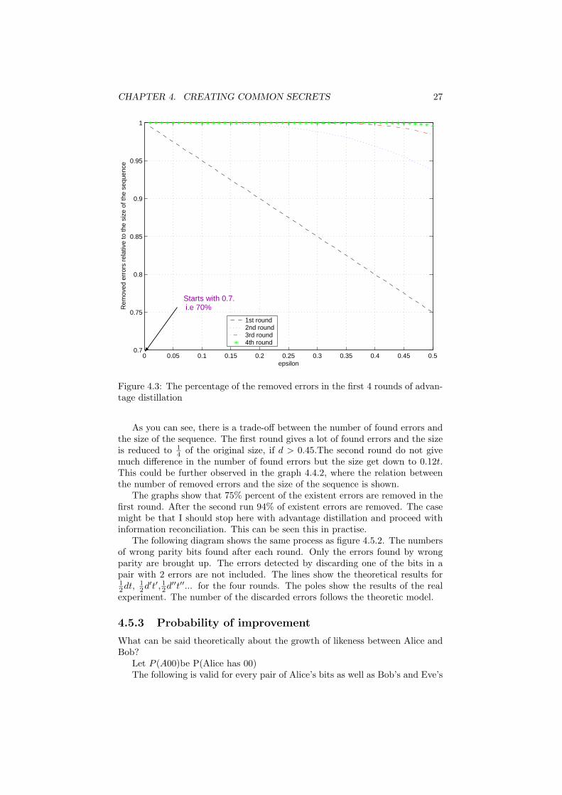
Figure 4.3: The percentage of the removed errors in the first 4 rounds of advan-tage distillation

As you can see, there is a trade-off between the number of found errors andthe size of the sequence. The first round gives a lot of found errors and the sizeis reduced to 1

4 of the original size, if d > 0.45.The second round do not givemuch difference in the number of found errors but the size get down to 0.12t.This could be further observed in the graph 4.4.2, where the relation betweenthe number of removed errors and the size of the sequence is shown.

The graphs show that 75% percent of the existent errors are removed in thefirst round. After the second run 94% of existent errors are removed. The casemight be that I should stop here with advantage distillation and proceed withinformation reconciliation. This can be seen this in practise.

The following diagram shows the same process as figure 4.5.2. The numbersof wrong parity bits found after each round. Only the errors found by wrongparity are brought up. The errors detected by discarding one of the bits in apair with 2 errors are not included. The lines show the theoretical results for12dt, 1

2d′t′, 12d′′t′′... for the four rounds. The poles show the results of the realexperiment. The number of the discarded errors follows the theoretic model.

4.5.3 Probability of improvement

What can be said theoretically about the growth of likeness between Alice andBob?

Let P (A00)be P(Alice has 00)The following is valid for every pair of Alice’s bits as well as Bob’s and Eve’s


0 0.05 0.1 0.15 0.2 0.25 0.3 0.35 0.4 0.45 0.50

500

1000

1500

2000

2500

3000

3500

Epsilon

Num

ber

of d

isca

rded

err

ors


Figure 4.4: Fig 4.4.3. The theoretical and the real number of errors discardedby removing pairs with odd number of errors


P (00) = 0.25 = P (01) = P (10) = P (11)The probability that Alice and Bob have the same pair of bits isP (A00)∧P (B00)+P (A10)∧P (B10)+P (A11)∧P (B11)+P (A01)∧P (B01) =

0.0625 ∗ 4 = 0.25The probability of having different bits is then 0.75.The probability that

Alice and Bob will have different bit after a parity bit is compared will be:P (The bits were different but the parities matched)P (A01)∧P (B10)+P (A00)∧P (B11)+P (A10)∧P (B01)+P (A11)∧P (B00)(0.25 ∗ 0.25 ∗ 4) = 0.25 (Se table 4.4.3)

4.5.4 How much information does Eve get

Eve gets the information about Alice’s bits and Bobs bits. She is able to listen tothe answer of the synchronizer, but she can compute it by herself. Now severalcases are possible. If all tree have the same parity, than the probability for Eveto get the right digit is the same as for Alice and Bob. That is 0.25 since thereis only 0.25 chance of having the same parity when the last digit differs.

A B m r/w11 00 m w11 01 mm11 10 mm11 11 m r00 00 m r00 01 mm00 10 mm00 11 m w01 00 mm01 01 m r01 10 m w01 11 mm10 00 mm10 01 m w10 10 m r10 11 mm

Table 4.4.3. The different combinations and the results. Match (m) and mismatch(mm) and right (r) or wrong (w) digit.

In case of a mismatch between Alice and Bob, Eve gets the same amount ofinformation as Bob, since she knows that the current two bits should be thrownaway. But here she is a loser by not being able to control the discarding, since ifshe has a match with one of the participants, she can not influence the sequenceas the other participant can.

In the case of a match between Alice and Bob, when Eves parity does notmatch she can only guess the answer and her information is not better thanguessing without listening.

4.6 The effects of the length of blocks

In the second phase of the given algorithm, Table-4.4.3.-The information recon-ciliation, you use a certain block size to compute parity over and send to the one


you want to create the key with. The size of these blocks effects the probabilityto correct errors and the amount of information Eve gets.

4.6.1 The probability

Let s be the block size, d- the block error, and ε−the fault rate. Then, theprobability of getting the odd number of errors in block is:

P (i errors in a block with lenght s) = (si ) ∗ εi(1− ε)s−i

P (to have an odd number of errors) = Σi is odd (si ) ∗ εi(1− ε)s−i

P (to have an odd number of errors) =(si ) (1− ε)s−i

Σi is odd (si ) ∗ εi(1− ε)s−i

s = 2-¿P (to have an odd number of errors) =P (1error) =2ε(1− ε)s = 3-¿P (tohaveanoddnumberof errors) =P (1error)+P (3errors)=3ε(1−

ε)+(32

)(1− ε)3−2

s = 4-¿P (tohaveanoddnumberof errors) =P (1error)+P (3errors)=4ε(1−ε)+

(42

)(1− ε)4−2

s = 5-¿P (to have an odd number of errors) =P (1error) + P (3errors) +P (5errors)

= Σi is odd

(5i

)∗ εi(1− ε)5−i

Let n ∈ ℵ={ 0,1,2,...} and i = 2*n+1. Then i ∈Odd natural numbers, {1,3,5...}.

The block length s starts with 2. s = n+2The maximum number of errors discovered in the block of length s is p( s

2 )q∗2− 1

P(to find error in the block of length s) = Σ(s−2)∗2+1i=1 (s

i ) ∗ εi(1− ε)s−i

Taking a closer look into the experiment which values was discussed andshown in 4.5.2 and fig 4.4.2 you can see that from the beginning I had 10000bits in the sequence built of 28thbits of measurement values. The number ofdifferences between the sequences is 2891. After the first round I find 1937blocks with odd number of errors and and I get rid of (2891-1937)/2 = 477errors “for free”. The number of error left for the second round is 477 and thenumber of bits left (the sequence length) is (10000-(2*1937))/2 = 3063. In thenext round I find 395 blocks with odd number of errors. I get rid of (477-395)/2= 41 errors. And if I stop the advantage distillation after this second round likeI suggested in 4.5.2 because more than 98 % of all the errors is gone I end upwith 41 errors in (3062 - (395*2))/2 = 1136 bits long sequence.

Let’s take a couple of examples. If I take a block length 20 in the phase ofinformation reconciliation I have:

P(to find error in the block of length s) = Σ(s−2)∗2+1i=1 (s

i ) ∗ εi(1− ε)s−i

Since one can theoretically predict the error rate in the sequence that ishanded over to the phase of information reconciliation one can make conclusionsabout the size of the block needed for a certain sequence. The greater the faultrate, the shorter block length I should pick. The trade-off here is like in the casesbefore that of Eve getting more information the shorter the block size is. Butin the same time if the fault rate, or difference, between Alice and Bob is biggerthan usual, the differences between Eve and the legal users can be expected tobe bigger than usual as well. A default value of the block size should be set andincreased or decreased depending on the calculated fault rate at that stage.

Chapter 5

Implementation

This chapter describes the main features of the implementation. Three differentmodules with some overlapping functions have been implemented. Those arethe compare module, the create key module and the test module. The first oneis only used to measure the changes in the differences between sequences. Thecreate key module is used for the key creation and in the test module all thestatistical tests of randomness are implemented.

5.1 Compare module

The compare module is used for the investigation and analysis of the sequencesbefore and after different steps in the main assignment. The program takes twofiles with measured or generated values, it constructs bit sequences as describedin figure 3.1 (chapter 2) and counts the number of differences for every bitbetween those two files. It also translates and writes down the values to binaryform to files if a flag is given.

5.2 Create key module

The module creates a secret key for two machines with two sequences (whichare values from a common measurement). It contains the process of exchangingthe messages to get information about the other part’s data and making theown data more alike the other one’s through synchronization. The synchronizermodule can also be installed on some other machine than the two who are inthe process of creating a common secret.

It starts and waits for some create key program to contact it. When thecommunication channel to one of the machines wishing to synchronize the se-quence is opened, only the machine with the ip-address of the machine the firstone want to synchronize data with is able to open a socket connection to thesynchronizer.

The messages exchanged are sent in tcp packets. Both of the participants,let us call them Alice and Bob, send their parity bits in a packet with a sequencenumber to the synchronizer. The synchronizer compares them and sends theresult that Alice and Bob respond to according to the algorithm (4.3). Thesecond phase of the algorithm is implemented in exactly the same way but the

31

CHAPTER 5. IMPLEMENTATION 32

parity at Alice’s and Bob’s are counted over a block larger than 2 bits. Also,since the participants do not throw away parts of the sequence but “repair”it, someone’s sequence has to be “the right one”. I decide that the one whosepacket arrived first is the right one, and hence the other one is the one who flipshis bits in case of parity mismatch.

5.3 Test module

The test module implements the decision of taking out a sequence for key con-struction. It exposes the measurement (or generated) values to the tests ofrandomness and returns the information about which bits from b0, b1, ...b31 canconstruct a sequence useful for key creation. If the measurement is shorterthan 384000 values only the five tests are applied. If it is longer than that, theuniversal Maurer’s test is applied.

Chapter 6

Conclusion/Discussion

6.1 Conclusions

One of the main conclusions I can make from this work is that it is both possibleto extract a binary sequence from the measurements and create a key by usinga public discussion algorithm[1].

In this work I looked at* extraction of a random enough sequence from the measurements of a pro-

cess* the similarity of 2 extracted pseudo random sequences when 2 entities do

the same measurement* implementation of the algorithm [1] to increase the similarity of the se-

quences and create a common key.Concerning extraction of the sequence I conclude that the bits that should be

used for creating a pseudo random sequence are number 28 and 29. Those buildsequences that both pass through the randomness tests and are alike enough toconverge in the reduction of the differences by the algorithm.

When it comes to implementation and analysing the algorithm for key cre-ation, one of the conclusions I make is that it is possible to theoretically calcu-late/predict how many bits are erased in each round of advantage distillation,what the error probability is after each round, and how many errors are left tothe second step.

Since reduction of the sequence length is huge in advantage distillation andafter the two rounds the algorithm removes more than 90 percent of errors theadvantage distillation should only run two rounds and leave the remaining errorsto be removed by the second step, information reconciliation.

Then the block size for the second step of the algorithm (information recon-ciliation) can be chosen with knowledge of the probable number of errors left.One of the conclusions I make is that you can go far in analysing this algorithmwhile only working with probabilities.

6.2 What can be done

Keeping track of what just been said, one can go a long way just counting withprobabilities in this analysis but a more proper and deep way to do this would

33

CHAPTER 6. CONCLUSION/DISCUSSION 34

involve information theoretical terms.Using information theory, entropy and the amount of information Eve gains

could be analysed more thoroughly. I was not able to estimate the amountof information she gets working with just probabilities, but it still could bethe case that deeper knowledge in statistics could give a better result. A deepinformation theoretical analysis of this can be found in [4].

Another thing that still remains to be analysed is the effect of the length ofthe blocks used in step 2 (information reconciliation) of the algorithm, which Ijust touched by expressing the probability of finding an odd number of errorsgiven the block length.

It would be interesting to look at whether an algorithm that makes a se-cret agreement by public discussion for more than two participants is possible.The present algorithm cannot be extended or generalised to involve more legalusers but the idea might be useful when constructing a suitable algorithm orheuristics.

I did not implement the last step, privacy amplification, due to the lack oftime.

Chapter 7

Appendix

7.1 Chi-square χ2 distribution. [4][6]

The χ2 distribution results when independent variables with standard normaldistributions are squared and summed. The χ2 distribution is typically usedto develop hypothesis tests and determining confidence intervals. Dependingon the shape parameter - degree of freedom df , the density function can lookvery differently. Following is the plot of the χ2probability density function for4 different degrees of freedom.

35

CHAPTER 7. APPENDIX 36

Figure 7.1: Chi-square distribution with 4 different degrees of freedom. (source:[6])

Bibliography

[1] Ueli M. Maurer. “Secret Key Agreement by Public Discussion From CommonInformation.

[2] A.Menezes, P.van Oorschot, S. Vanstone. “Handbook of Applied Cryptog-raphy.”

[3] “Secret Key Agreement by Public Discussion”. Ueli M. Mau-rer. Information Security and Cryptography. Can be found athttp://www.crypto.ethz.ch/research/keydemo

[4] Ueli M. Maurer. “Secret-Key Agreement over Unauthenticated Public Chan-nels - Part I: Definitions and a completeness result.”

[5] “Sannolikhetsteori och statistikteori med tillampningar.” Gunnar Blom.

[6] Chi-Square Distribution. Engineering statistics handbook. Can be found athttp://www.itl.nist.gov/div898/handbook/eda/section3/eda3666.htm

37

from probability distributions to common secrets · to common secrets anna otto june 2004. 1...

Documents