from random matrix theory to number theory

Introduction Classical RMT Intro to L-Function Dirichlet L-functions Cuspidal Newforms Refs

From Random Matrix Theoryto Number Theory

Steven J MillerWilliams College

[email protected]://www.williams.edu/go/math/sjmiller/

Graduate Workshop on Zeta Functions,L-Functions and their ApplicationsUtah Valley University, June 2009

1


Goals

Determine correct scale and statistics to study zerosof L-functions.

See similar behavior in different systems.

Discuss the tools and techniques needed to prove theresults.

2


Introduction

3


Fundamental Problem: Spacing Between Events

General Formulation: Studying system, observe values att1, t2, t3, . . . .

Question: What rules govern the spacings between the ti?

Examples:

Spacings b/w Energy Levels of Nuclei.Spacings b/w Eigenvalues of Matrices.Spacings b/w Primes.Spacings b/w nkα mod 1.Spacings b/w Zeros of L-functions.

4


Sketch of proofs

In studying many statistics, often three key steps:

1 Determine correct scale for events.

2 Develop an explicit formula relating what we want tostudy to something we understand.

3 Use an averaging formula to analyze the quantitiesabove.

It is not always trivial to figure out what is the correctstatistic to study!

5


ClassicalRandom Matrix Theory

6


Origins of Random Matrix Theory

Classical Mechanics: 3 Body Problem Intractable.

Heavy nuclei (Uranium: 200+ protons / neutrons) worse!

Get some info by shooting high-energy neutrons intonucleus, see what comes out.

Fundamental Equation:

Hψn = Enψn

H : matrix, entries depend on systemEn : energy levelsψn : energy eigenfunctions

7


Origins (continued)

Statistical Mechanics: for each configuration,calculate quantity (say pressure).Average over all configurations – most configurationsclose to system average.Nuclear physics: choose matrix at random, calculateeigenvalues, average over matrices (real SymmetricA = AT , complex Hermitian A

T= A).

8


Random Matrix Ensembles

A =

a11 a12 a13 · · · a1N

a12 a22 a23 · · · a2N...

......

. . ....

a1N a2N a3N · · · aNN

= AT , aij = aji

Fix p, define

Prob(A) =∏

1≤i≤j≤N

p(aij).

This means

Prob (A : aij ∈ [αij , βij ]) =∏

1≤i≤j≤N

∫ βij

xij=αij

p(xij)dxij .

Want to understand eigenvalues of A.9


Eigenvalue Distribution

δ(x − x0) is a unit point mass at x0.

To each A, attach a probability measure:

µA,N(x) =1N

N∑

i=1

δ

(x − λi(A)

2√

N

)

∫ b

aµA,N(x)dx =

#{λi : λi(A)

2√

N∈ [a, b]

}

N

kth moment =

∑Ni=1 λi(A)k

2kNk2 +1

=Trace(Ak )

2k Nk2 +1

.

10


Wigner’s Semi-Circle Law

Wigner’s Semi-Circle Law

N × N real symmetric matrices, entries i.i.d.r.v. from afixed p(x) with mean 0, variance 1, and other momentsfinite. Then for almost all A, as N →∞

µA,N(x) −→{

2π

√1− x2 if |x | ≤ 1

0 otherwise.

11


SKETCH OF PROOF: Eigenvalue Trace Lemma

Want to understand the eigenvalues of A, but it is thematrix elements that are chosen randomly andindependently.

Eigenvalue Trace Lemma

Let A be an N × N matrix with eigenvalues λi(A). Then

Trace(Ak ) =N∑

n=1

λi(A)k ,

where

Trace(Ak) =N∑

i1=1

· · ·N∑

ik=1

ai1i2ai2i3 · · ·aiN i1.

12


SKETCH OF PROOF: Correct Scale

Trace(A2) =N∑

i=1

λi(A)2.

By the Central Limit Theorem:

Trace(A2) =

N∑

i=1

N∑

j=1

aijaji =

N∑

i=1

N∑

j=1

a2ij ∼ N2

N∑

i=1

λi(A)2 ∼ N2

Gives NAve(λi(A)2) ∼ N2 or Ave(λi(A)) ∼√

N.

13


SKETCH OF PROOF: Averaging Formula

Recall k -th moment of µA,N(x) is Trace(Ak )/2kNk/2+1.

Average k -th moment is∫· · ·∫

Trace(Ak)

2kNk/2+1

∏

i≤j

p(aij)daij .

Proof by method of moments: Two steps

Show average of k -th moments converge to momentsof semi-circle as N →∞;Control variance (show it tends to zero as N →∞).

14


SKETCH OF PROOF: Averaging Formula for Second Moment

Substituting into expansion gives

122N2

∫ ∞

−∞· · ·∫ ∞

−∞

N∑

i=1

N∑

j=1

a2ji · p(a11)da11 · · ·p(aNN)daNN

Integration factors as∫ ∞

aij=−∞a2

ij p(aij)daij ·∏

(k,l) 6=(i,j)k<l

∫ ∞

akl=−∞p(akl)dakl = 1.

Higher moments involve more advanced combinatorics(Catalan numbers).

15


SKETCH OF PROOF: Averaging Formula for Higher Moments

Higher moments involve more advanced combinatorics(Catalan numbers).

12k Nk/2+1

∫ ∞

−∞· · ·∫ ∞

−∞

N∑

i1=1

· · ·N∑

ik=1

ai1i2 · · ·aik i1 ·∏

i≤j

p(aij)daij .

Main contribution when the aiℓiℓ+1 ’s matched in pairs, notall matchings contribute equally (if did would get aGaussian and not a semi-circle; this is seen in RealSymmetric Palindromic Toeplitz matrices).

16


Numerical examples

−1.5 −1 −0.5 0 0.5 1 1.50

0.005

0.01

0.015

0.02

0.025Distribution of eigenvalues−−Gaussian, N=400, 500 matrices

500 Matrices: Gaussian 400× 400p(x) = 1√

2πe−x2/2

17


Numerical examples

−300 −200 −100 0 100 200 3000

500

1000

1500

2000

2500

The eigenvalues of the Cauchydistribution are NOT semicirular.

Cauchy Distribution: p(x) = 1π(1+x2)

18


Introductionto L-Functions

19


Riemann Zeta Function

ζ(s) =∞∑

n=1

1ns

=∏

p prime

(1− 1

ps

)−1

, Re(s) > 1.

Functional Equation:

ξ(s) = Γ(s

2

)π− s

2 ζ(s) = ξ(1− s).

Riemann Hypothesis (RH):

All non-trivial zeros have Re(s) =12

; can write zeros as12

+iγ.

Observation: Spacings b/w zeros appear same as b/weigenvalues of Complex Hermitian matrices A

T= A.

20


Zeros of ζ(s) vs GUE

70 million spacings b/w adjacent zeros of ζ(s), starting atthe 1020th zero (from Odlyzko)

21


Explicit Formula (Contour Integration)

−ζ′(s)

ζ(s)= − d

dslog ζ(s)

=dds

∑

p

log(1− p−s

)

=∑

p

log p · p−s

1− p−s=∑

p

log pps

+ Good(s).

Contour Integration:∫− ζ ′(s)

ζ(s)

xs

sds vs

∑

p

log p∫ (

xp

)s dss.

Knowledge of zeros gives info on coefficients.22


Measures of Spacings: n-Level Correlations

{αj} increasing sequence, box B ⊂ Rn−1.

n-level correlation

limN→∞

#

{(αj1 − αj2 , . . . , αjn−1 − αjn

)∈ B, ji 6= jk

}

N

(Instead of using a box, can use a smooth test function.)

23


Measures of Spacings: n-Level Correlations

{αj} increasing sequence, box B ⊂ Rn−1.

1 Normalized spacings of ζ(s) starting at 1020

(Odlyzko).2 2 and 3-correlations of ζ(s) (Montgomery, Hejhal).3 n-level correlations for all automorphic cupsidal

L-functions (Rudnick-Sarnak).4 n-level correlations for the classical compact groups

(Katz-Sarnak).5 Insensitive to any finite set of zeros.

24


Measures of Spacings: n-Level Density and Families

φ(x) :=∏

i φi(xi), φi even Schwartz functions whoseFourier Transforms are compactly supported.

n-level density

Dn,f (φ) =∑

j1,...,jndistinct

φ1

(Lfγ

(j1)f

)· · ·φn

(Lfγ

(jn)f

)

1 Individual zeros contribute in limit.2 Most of contribution is from low zeros.3 Average over similar curves (family).

Katz-Sarnak ConjecturesFor a ‘nice’ family of L-functions, the n-level densitydepends only on a symmetry group attached to the family.

25


Normalization of Zeros

Local (hard, use Cf ) vs Global (easier, use log C =|FN |−1

∑f∈FN

log Cf ). Hope: φ a good even test functionwith compact support, as |F| → ∞,

1|F|N

∑

f∈FN

Dn,f (φ) =1|F|N

∑

f∈FN

∑

j1,...,jnji 6=±jk

∏

i

φi

(log Cf

2πγ

(ji )E

)

→∫· · ·∫φ(x)Wn,G(F)(x)dx .

Katz-Sarnak Conjecture

As Cf →∞ the behavior of zeros near 1/2 agrees withN →∞ limit of eigenvalues of a classical compact group.

26


1-Level Densities

The Fourier Transforms for the 1-level densities are

W1,SO(even)(u) = δ0(u) +12η(u)

W1,SO(u) = δ0(u) +12

W1,SO(odd)(u) = δ0(u)− 12η(u) + 1

W1,Sp(u) = δ0(u)− 12η(u)

W1,U(u) = δ0(u)

where δ0(u) is the Dirac Delta functional and

η(u) =

{ 1 if |u| < 112 if |u| = 10 if |u| > 1

27


Correspondences

Similarities between L-Functions and Nuclei:

Zeros ←→ Energy Levels

Support of test function ←→ Neutron Energy.

28


Some Number Theory Results

Orthogonal: Iwaniec-Luo-Sarnak, Ricotta-Royer:1-level density for holomorphic even weight kcuspidal newforms of square-free level N (SO(even)and SO(odd) if split by sign).Symplectic: Rubinstein, Gao: n-level densities fortwists L(s, χd) of the zeta-function.Unitary: Miller, Hughes-Rudnick: Families of PrimitiveDirichlet Characters.Orthogonal: Miller, Young: One and two-parameterfamilies of elliptic curves.

29


Main Tools

1 Control of conductors: Usually monotone, gives scaleto study low-lying zeros.

2 Explicit Formula: Relates sums over zeros to sumsover primes.

3 Averaging Formulas: Petersson formula inIwaniec-Luo-Sarnak, Orthogonality of characters inRubinstein, Miller, Hughes-Rudnick.

30


Example:Dirichlet L-functions

31


Dirichlet Characters

(Z/mZ)∗ is cyclic of order m − 1 with generator g. Letζm−1 = e2πi/(m−1). The principal character χ0 is given by

χ0(k) =

{1 (k ,m) = 10 (k ,m) > 1.

The m − 2 primitive characters are determined (bymultiplicativity) by action on g.

As each χ : (Z/mZ)∗ → C∗, for each χ there exists an lsuch that χ(g) = ζ l

m−1. Hence for each l , 1 ≤ l ≤ m− 2 wehave

χl(k) =

{ζ la

m−1 k ≡ ga(m)

0 (k ,m) > 0

32


Dirichlet L-Functions

Let χ be a primitive character mod m. Let

c(m, χ) =

m−1∑

k=0

χ(k)e2πik/m.

c(m, χ) is a Gauss sum of modulus√

m.

L(s, χ) =∏

p

(1− χ(p)p−s)−1

Λ(s, χ) = π− 12 (s+ǫ)Γ

(s + ǫ

2

)m

12 (s+ǫ)L(s, χ),

where

ǫ =

{0 if χ(−1) = 11 if χ(−1) = −1

c(m, χ)33


Explicit Formula

Let φ be an even Schwartz function with compact support(−σ, σ), let χ be a non-trivial primitive Dirichlet characterof conductor m.

∑φ

(γ

log(mπ)

2π

)

=

∫ ∞

−∞φ(y)dy

−∑

p

log plog(m/π)

φ( log p

log(m/π)

)[χ(p) + χ(p)]p− 1

2

−∑

p

log plog(m/π)

φ(

2log p

log(m/π)

)[χ2(p) + χ2(p)]p−1

+O( 1

log m

).

34


Expansion

{χ0} ∪ {χl}1≤l≤m−2 are all the characters mod m.Consider the family of primitive characters mod a prime m(m − 2 characters):

∫ ∞

−∞φ(y)dy

− 1m − 2

∑

χ 6=χ0

∑

p

log plog(m/π)

φ( log p

log(m/π)

)[χ(p) + χ(p)]p− 1

2

− 1m − 2

∑

χ 6=χ0

∑

p

log plog(m/π)

φ(

2log p

log(m/π)

)[χ2(p) + χ2(p)]p−1

+ O( 1

log m

).

Note can pass Character Sum through Test Function.35


Character Sums

∑

χ

χ(k) =

{m − 1 k ≡ 1(m)

0 otherwise.

For any prime p 6= m

∑

χ 6=χ0

χ(p) =

{m − 1− 1 p ≡ 1(m)

−1 otherwise.

Substitute into

1m − 2

∑

χ 6=χ0

∑

p

log plog(m/π)

φ( log p

log(m/π)

)[χ(p) + χ(p)]p− 1

2

36


First Sum: no contribution if σ < 2

−2m − 2

mσ∑

p

log plog(m/π)

φ( log p

log(m/π)

)p− 1

2

+ 2m − 1m − 2

mσ∑

p≡1(m)

log plog(m/π)

φ( log p

log(m/π)

)p− 1

2

≪ 1m

mσ∑

p

p− 12 +

mσ∑

p≡1(m)

p− 12 ≪ 1

m

mσ∑

k

k− 12 +

mσ∑

k≡1(m)k≥m+1

k− 12

≪ 1m

mσ∑

k

k− 12 +

1m

mσ∑

k

k− 12 ≪ 1

mmσ/2.

37


Second Sum

1m − 2

∑

χ 6=χ0

∑

p

log plog(m/π)

φ(

2log p

log(m/π)

)χ2(p) + χ2(p)

p.

∑

χ 6=χ0

[χ2(p) + χ2(p)] =

{2(m − 2) p ≡ ±1(m)

−2 p 6≡ ±1(m)

Up to O(

1log m

)we find that

≪ 1m − 2

mσ/2∑

p

p−1 +2m − 2m − 2

mσ/2∑

p≡±1(m)

p−1

≪ 1m − 2

mσ/2∑

k

k−1 +

mσ/2∑

k≡1(m)k≥m+1

k−1 +

mσ/2∑

k≡−1(m)k≥m−1

k−1

38


Dirichlet Characters: m Square-free

Fix an r and let m1, . . . ,mr be distinct odd primes.

m = m1m2 · · ·mr

M1 = (m1 − 1)(m2 − 1) · · · (mr − 1) = φ(m)

M2 = (m1 − 2)(m2 − 2) · · · (mr − 2).

M2 is the number of primitive characters mod m, each ofconductor m. A general primitive character mod m isgiven by χ(u) = χl1(u)χl2(u) · · ·χlr (u). LetF = {χ : χ = χl1χl2 · · ·χlr}.

1M2

∑

p

log plog(m/π)

φ( log p

log(m/π)

)p− 1

2

∑

χ∈F[χ(p) + χ(p)]

1M2

∑

p

log plog(m/π)

φ(

2log p

log(m/π)

)p−1

∑

χ∈F[χ2(p) + χ2(p)]

39


Characters Sums

mi−2∑

li=1

χli (p) =

{mi − 1− 1 p ≡ 1(mi)

−1 otherwise.

Define

δmi (p, 1) =

{1 p ≡ 1(mi)

0 otherwise.

Then∑

χ∈Fχ(p) =

m1−2∑

l1=1

· · ·mr−2∑

lr =1

χl1(p) · · ·χlr (p)

=

r∏

i=1

mi−2∑

li=1

χli (p) =

r∏

i=1

(− 1 + (mi − 1)δmi (p, 1)

).

40


Expansion Preliminaries

k(s) is an s-tuple (k1, k2, . . . , ks) with k1 < k2 < · · · < ks.This is just a subset of (1, 2, . . . , r), 2r possible choices fork(s).

δk(s)(p, 1) =

s∏

i=1

δmki(p, 1).

If s = 0 we define δk(0)(p, 1) = 1 ∀p.Then

r∏

i=1

(− 1 + (mi − 1)δmi (p, 1)

)

=r∑

s=0

∑

k(s)

(−1)r−sδk(s)(p, 1)s∏

i=1

(mki − 1).

41


First Sum

≪mσ∑

p

p− 12

1M2

(1 +

r∑

s=1

∑

k(s)

δk(s)(p, 1)

s∏

i=1

(mki − 1)).

As m/M2 ≤ 3r , s = 0 sum contributes

S1,0 =1

M2

mσ∑

p

p− 12 ≪ 3r m

12 σ−1,

hence negligible for σ < 2.

42


First Sum

≪mσ∑

p

p− 12

1M2

(1 +

r∑

s=1

∑

k(s)

δk(s)(p, 1)

s∏

i=1

(mki − 1)).

Now we study

S1,k(s) =1

M2

s∏

i=1

(mki − 1)

mσ∑

p

p− 12 δk(s)(p, 1)

≪ 1M2

s∏

i=1

(mki − 1)

mσ∑

n≡1(mk(s))

n− 12

≪ 1M2

s∏

i=1

(mki − 1)1∏s

i=1(mki )

mσ∑

n

n− 12 ≪ 3r m

12 σ−1.

43


First Sum (continued)

There are 2r choices, yielding

S1 ≪ 6r m12 σ−1,

which is negligible as m goes to infinity for fixed r if σ < 2.Cannot let r go to infinity.If m is the product of the first r primes,

log m =

r∑

k=1

log pk

=∑

p≤r

log p ≈ r

Therefore6r ≈ mlog 6 ≈ m1.79.

44


Second Sum Expansions

mi−2∑

li=1

χ2li (p) =

{mi − 1− 1 p ≡ ±1(mi)

−1 otherwise

∑

χ∈Fχ2(p) =

m1−2∑

l1=1

· · ·mr−2∑

lr =1

χ2l1(p) · · ·χ2

lr (p)

=r∏

i=1

mi−2∑

li=1

χ2li (p)

=

r∏

i=1

(− 1 + (mi − 1)δmi (p, 1) + (mi − 1)δmi (p,−1)

).

45


Second Sum Bounds

Handle similarly as before. Say

p ≡ 1 mod mk1 , . . . ,mka

p ≡ −1 mod mka+1, . . . ,mkb

How small can p be?+1 congruences imply p ≥ mk1 · · ·mka + 1.−1 congruences imply p ≥ mka+1 · · ·mkb − 1.Since the product of these two lower bounds is greaterthan

∏bi=1(mki − 1), at least one must be greater than

(∏bi=1(mki − 1)

) 12.

There are 3r pairs, yielding

Second Sum =r∑

s=0

∑

k(s)

∑

j(s)

S2,k(s),j(s) ≪ 9r m− 12 .

46


Summary

Agrees with Unitary for σ < 2 for square-free m ∈ [N, 2N]from:

Theoremm square-free odd integer with r = r(m) factors;m =

∏ri=1 mi ;

M2 =∏r

i=1(mi − 2).

Then family Fm of primitive characters mod m has

First Sum ≪ 1M2

2r m12 σ

Second Sum ≪ 1M2

3r m12 .

47


CuspidalNewforms

48


Results from Iwaniec-Luo-Sarnak

Orthogonal: Iwaniec-Luo-Sarnak: 1-level density forholomorphic even weight k cuspidal newforms ofsquare-free level N (SO(even) and SO(odd) if split bysign).

Symplectic: Iwaniec-Luo-Sarnak: 1-level density forsym2(f ), f holomorphic cuspidal newform.

Will review Orthogonal case and talk about extensions(joint with Chris Hughes).

49


Modular Form Preliminaries

Γ0(N) =

{(a bc d

):

ad − bc = 1c ≡ 0(N)

}

f is a weight k holomorphic cuspform of level N if

∀γ ∈ Γ0(N), f (γz) = (cz + d)k f (z).

Fourier Expansion: f (z) =∑∞

n=1 af (n)e2πiz ,L(s, f ) =

∑∞n=1 ann−s.

Petersson Norm: 〈f , g〉 =∫Γ0(N)\H f (z)g(z)y k−2dxdy .

Normalized coefficients:

ψf (n) =

√Γ(k − 1)

(4πn)k−1

1||f ||af (n).

50


Petersson Formula

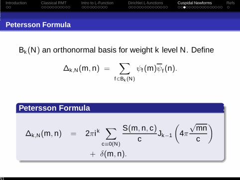
Bk (N) an orthonormal basis for weight k level N. Define

∆k ,N(m, n) =∑

f∈Bk (N)

ψf (m)ψf (n).

Petersson Formula

∆k ,N(m, n) = 2πik∑

c≡0(N)

S(m, n, c)

cJk−1

(4π

√mnc

)

+ δ(m, n).

51


Fourier Coefficient Review

λf (n) = af (n)nk−1

2

λf (m)λf (n) =∑

d|(m,n)(d,M)=1

λf

(mnd

).

For a newform of level N, λf (N) is trivially related to thesign of the form:

ǫf = ikµ(N)λf (N)√

N.

The above will allow us to split into even and odd families:1± ǫf .

52


Key Kloosterman-Bessel integral from ILS

Ramanujan sum:

R(n, q) =∑∗

a mod q

e(an/q) =∑

d |(n,q)

µ(q/d)d ,

where ∗ restricts the summation to be over all a relativelyprime to q.

Theorem (ILS)

Let Ψ be an even Schwartz function with supp(Ψ) ⊂ (−2, 2). Then

∑

m≤Nǫ

1

m2

∑

(b,N)=1

R(m2, b)R(1, b)

ϕ(b)

∫∞

y=0Jk−1(y)Ψ

(2 log(by

√N/4πm)

log R

)dy

log R

= −1

2

[∫∞

−∞Ψ(x)

sin 2πx

2πxdx −

1

2Ψ(0)

]+ O

(k log log kN

log kN

),

where R = k2N and ϕ is Euler’s totient function.

53


Limited Support ( σ < 1): Sketch of proof

Estimate Kloosterman-Bessel terms trivially.⋄ Kloosterman sum: dd ≡ 1 mod q, τ(q) is thenumber of divisors of q,

S(m, n; q) =∑∗

d mod q

e

(mdq

+ndq

)

|S(m, n; q)| ≤ (m, n, q)

√

min{

q(m, q)

,q

(n, q)

}τ(q).

⋄ Bessel function: integer k ≥ 2,Jk−1(x)≪ min

(x , xk−1, x−1/2

).

Use Fourier Coefficients to split by sign: N fixed:±∑f λf (N) ∗ (· · · ).

54


Increasing Support ( σ < 2): Sketch of the proof

Using Dirichlet Characters, handle Kloostermanterms.

Have terms like∫ ∞

0Jk−1

(4π

√m2yNc

)φ

(log ylog R

)dy√

y

with arithmetic factors to sum outside.

Works for support up to 2.

55


Increasing Support ( σ < 2): Kloosterman-Bessel details

Stating in greater generality for later use.

Gauss sum: χ a character modulo q: |Gχ(n)| ≤ √q with

Gχ(n) =∑

a mod q

χ(a) exp(2πian/q).

56


Increasing Support ( σ < 2): Kloosterman-Bessel details

Kloosterman expansion:

S(m2, p1 · · ·pnN; Nb)

=−1ϕ(b)

∑

χ(mod b)

χ(N)Gχ(m2)Gχ(1)χ(p1 · · ·pn).

Lemma: Assuming GRH for Dirichlet L-functions,supp(φ) ⊂

(−2

n ,2n

), non-principal characters negligible.

Proof: use Jk−1(x)≪ x and see

≪ 1√N

∑

m≤Nǫ

1m

∑

(b,N)=1b<N2006

1b

1ϕ(b)

∑

χ(mod b)χ6=χ0

∣∣Gχ(m2)Gχ(1)∣∣

× m

b√

N

n∏

j=1

∣∣∣∣∣∣

∑

pj 6=N

χ(pj) log pj ·1

log Rφ

(log pj

log R

)∣∣∣∣∣∣.

57


2-Level Density

∫ Rσ

x1=2

∫ Rσ

x2=2φ

(log x1

log R

)φ

(log x2

log R

)Jk−1

(4π

√m2x1x2N

c

)dx1dx2√

x1x2

Change of variables and Jacobean:

u2 = x1x2 x2 = u2u1

u1 = x1 x1 = u1

∣∣∣∣∂x∂u

∣∣∣∣ =

∣∣∣∣∣1 0−u2

u21

1u1

∣∣∣∣∣ =1u1.

Left with∫ ∫

φ

(log u1

log R

)φ

log(

u2u1

)

log R

1√

u2Jk−1

(4π

√m2u2N

c

)du1du2

u1

58


2-Level Density (continued)

Changing variables, u1-integral is∫ σ

w1=log u2log R −σ

φ (w1) φ

(log u2

log R− w1

)dw1.

Support conditions imply

Ψ2

(log u2

log R

)=

∫ ∞

w1=−∞φ (w1) φ

(log u2

log R− w1

)dw1.

Substituting gives∫ ∞

u2=0Jk−1

(4π

√m2u2N

c

)Ψ2

(log u2

log R

)du2√

u2

59


3-Level Density

∫ Rσ

x1=2

∫ Rσ

x2=2

∫ Rσ

x3=2φ

(log x1

log R

)φ

(log x2

log R

)φ

(log x3

log R

)

∗ Jk−1

(4π

√m2x1x2x3N

c

)dx1dx2dx3√

x1x2x3

Change variables as below and get Jacobean:

u3 = x1x2x3 x3 = u3u2

u2 = x1x2 x2 = u2u1

u1 = x1 x1 = u1

∣∣∣∣∂x∂u

∣∣∣∣ =

∣∣∣∣∣∣∣

1 0 0−u2

u21

1u1

0

0 −u3u2

2

1u2

∣∣∣∣∣∣∣=

1u1u2

.

60


n-Level Density: Determinant Expansions from RMT

U(N), Uk(N): det(

K0(xj , xk))

1≤j ,k≤n

USp(N): det(

K−1(xj , xk))

1≤j ,k≤n

SO(even): det(

K1(xj , xk))

1≤j ,k≤n

SO(odd): det (K−1(xj , xk))1≤j ,k≤n +∑n

ν=1 δ(xν) det(

K−1(xj , xk))

1≤j ,k 6=ν≤n

where

Kǫ(x , y) =sin(π(x − y)

)

π(x − y)+ ǫ

sin(π(x + y)

)

π(x + y).

61


n-Level Density: Sketch of proof

Expand Bessel-Kloosterman piece, use GRH to dropnon-principal characters, change variables, main term is

b√

N2πm

∫ ∞

0Jk−1(x)Φn

(2 log(bx

√N/4πm)

log R

)dx

log R

with Φn(x) = φ(x)n.

Main IdeaDifficulty in comparison with classical RMT is that insteadof having an n-dimensional integral of φ1(x1) · · ·φn(xn) wehave a 1-dimensional integral of a new test function. Thisleads to harder combinatorics but allows us to appeal tothe result from ILS.

62


Support for n-Level Density

Careful book-keeping gives (originally just had 1n−1/2 )

σn <1

n − 1.

n-Level Density is trivial for σn <1n , non-trivial up to 1

n−1 .

Expected 2n . Obstruction from partial summation on

primes.

63


Support Problems: 2-Level Density

Partial Summation on p1 first, looks like

∑

p1p1 6=p2

S(m2, p1p2N, c)2 log p1√p1 log R

φ

(log p1

log R

)Jk−1

(4π

√m2p1p2N

c

)

Similar to ILS, obtain (c = bN):∑

p1≤x1p1∤b

S(m2, p1p2N, c)log p√

p=

2µ(N)

φ(b)R(m2, b, p2)x

12

1 +O (b(bx1N)ǫ)

∑p1

to∫

x1, error≪ b(bN)ǫm

√p2NNσ2/2/bN, yields

√N∑

m≤Nǫ

1m

∑

b≤N5

1bN

∑

p2≤Nσ2

1√p2

b(bN)ǫm√

p2NNσ22

bN

≪ N12 +ǫ′+σ2+

12+

σ22 −2 ≪ N

32 σ2−1+ǫ′

64


Support Problems: n-Level Density: Why is σ2 < 1?

If no∑

p2, have above without the Nσ which arose

from∑

p2, giving

≪ N12+ǫ′+ 1

2 +σ12 −2 = N

12 σ1−1+ǫ′.

Fine for σ1 < 2. For 3-Level, have two sums overprimes giving Nσ3, giving

≪ N12 +ǫ′+2σ3+

12 +

σ32 −2 = N

52 σ3−1+ǫ′

n-Level, have an additional (n − 1) prime sums, eachgiving Nσn , yields

≪ N12 +ǫ′+(n−1)σn+ 1

2 + σn2 −2 = N

(2n−1)2 σn−1+ǫ′

65


Summary

More support for RMT Conjectures.

Control of Conductors.

Averaging Formulas.

Theorem (Hughes-Miller)

n-level densities of weight k cuspidal newforms of primelevel N, N →∞, agree with orthogonal in non-trivialrange (with or without splitting by sign).

66


Bibliography

67


B. Conrey, D. Farmer, P. Keating, M. Rubinstein and N. Snaith, Integral Moments of L-Functions, Proc. Lond.Math. Soc. 91 (2005), 33–104.

H. Davenport, Multiplicative Number Theory, 3rd edition, Graduate Texts in Mathematics 74, Springer-Verlag,New York, 2000, revised by H. Montgomery.

E. Dueñez and S. J. Miller, The Low Lying Zeros of a GL4 and a GL6 family of L-functions (preprint)arxiv.org/abs/math.NT/0506462.

E. Fouvry and H. Iwaniec, Low-lying zeros of dihedral L-functions, Duke Math. J. 116 (2003), 189–217.

P. Gao, N-level density of the low-lying zeros of quadratic Dirichlet L-functions, Ph. D thesis, University ofMichigan, 2005.

68


A. Güloglu, Low Lying Zeros of Symmetric Power L-Functions, Internat. Math. Res. Notices (2005), no. 9,517–550.

D. Hejhal, On the triple correlation of zeros of the zeta function, Internat. Math. Res. Notices (1994), no. 7,294–302.

J. Hoffstein and P. Lockhart, Coefficients of Maass forms and the Siegel zero. With an appendix by DorianGoldfeld, Hoffstein and Daniel Lieman, Ann. of Math. (2) 140 (1994), no. 1, 161–181.

C. Hughes and Z. Rudnick, Mock Gaussian behaviour for linear statistics of classical compact groups, J.Phys. A 36 (2003), 2919–2932.

C. Hughes and Z. Rudnick, Linear Statistics of Low-Lying Zeros of L-functions, Quart. J. Math. Oxford 54(2003), 309–333.

69


H. Iwaniec, Small eigenvalues of Laplacian for Γ0(N), Acta Arith. 56 (1990), no. 1, 65–82.

H. Iwaniec, Topics in Classical Automorphic Forms, Graduate Texts in Mathematics 17, AMS, Providence,1997.

H. Iwaniec, W. Luo and P. Sarnak, Low lying zeros of families of L-functions, Inst. Hautes Études Sci. Publ.Math. 91 (2000), 55–131.

N. Katz and P. Sarnak, Random Matrices, Frobenius Eigenvalues and Monodromy, AMS ColloquiumPublications 45, AMS, Providence, 1999.

N. Katz and P. Sarnak, Zeros of zeta functions and symmetries, Bull. AMS 36 (1999), 1–26.

70


J. P. Keating and N. C. Snaith, Random matrices and L-functions, Random matrix theory, J. Phys. A 36(2003), 2859–2881.

S. J. Miller, 1- and 2-Level Densities for Families of lliptic Curves: Evidence for the Underlying GroupSymmetries, Ph.D. Thesis, Princeton University, 2002,http://www.math.princeton.edu/∼sjmiller/thesis/thesis.pdf.

S. J. Miller, 1- and 2-Level Densities for Families of Elliptic Curves: Evidence for the Underlying GroupSymmetries, Compositio Mathematica 104 (2004), 952–992.

H. Montgomery, The pair correlation of zeros of the zeta function, Analytic Number Theory, Proc. Sympos.Pure Math. AMS 24 (1973), 181–193.

E. Royer, Petits zéros de fonctions L de formes modulaires, Acta Arith. 99 (2001), 47–172.

71


M. Rubinstein, Low-lying zeros of L-functions and random matrix theory, Duke Math. J. 109 (2001), 147–181.

Z. Rudnick and P. Sarnak, Zeros of principal L-functions and random matrix theory, Duke Math. J. 81 (1996),269–322.

E. C. Titchmarsh, The Theory of the Riemann Zeta-Function 2nd ed., revised by D. R. Heath-Brown, OxfordScience Publications, 1986.

A. Soshnikov, Central limit theorem for local linear statistics in classical compact groups and relatedcombinatorial identities, Ann. Probab. 28 (2000), 1353–1370.

G. N. Watson, A Treatise on the Theory of Bessel Functions, second edition, Cambridge University Press,1966.

M. Young, Low Lying Zeros of Families of Elliptic Curves, J. Amer. Math. Soc. 19 (2006), no. 1, 205–250.

72

from random matrix theory to number theory

Documents