Computing the Least Common Subsumer

w.r.t. a Background Terminology 1

Franz Baader ∗, Baris Sertkaya, Anni-Yasmin Turhan

Theoretical Computer Science, TU Dresden, Germany

Abstract

Methods for computing the least common subsumer (lcs) are usually restricted torather inexpressive Description Logics (DLs) whereas existing knowledge bases arewritten in very expressive DLs. In order to allow the user to re-use concepts definedin such terminologies and still support the definition of new concepts by computingthe lcs, we extend the notion of the lcs of concept descriptions to the notion of thelcs w.r.t. a background terminology. We will show both theoretical results on theexistence of the least common subsumer in this setting, and describe a practicalapproach—based on a method from formal concept analysis—for computing goodcommon subsumers, which may, however, not be the least ones. We will also describeresults obtained in a first evaluation of this practical approach.

Key words: Description Logic, Non-standard Inferences

1 Introduction

Description Logics (DLs) [1] are a class of knowledge representation formalismsin the tradition of semantic networks and frames, which can be used to repre-sent the terminological knowledge of an application domain in a structured andformally well-understood way. The name description logics is motivated by thefact that, on the one hand, the important notions of the domain are describedby concept descriptions, i.e., expressions that are built from atomic concepts

∗ Corresponding AuthorEmail addresses: baader@tcs.inf.tu-dresden.de (Franz Baader),

sertkaya@tcs.inf.tu-dresden.de (Baris Sertkaya),turhan@tcs.inf.tu-dresden.de (Anni-Yasmin Turhan).1 This work was supported by the German Science Foundation (DFG) under thegrants GRK 334/3 and BA 1122/4-4.

Preprint submitted to Elsevier Science 4 December 2006

(unary predicates) and atomic roles (binary predicates) using the concept androle constructors provided by the particular DL. On the other hand, DLs differfrom their predecessors, such as semantic networks and frames [2,3], in thatthey are equipped with a formal, logic-based semantics, which can, e.g., begiven by a translation into first-order predicate logic.

Knowledge representation systems based on description logics (DL systems)[4,5] provide their users with various inference capabilities that allow them todeduce implicit knowledge from the explicitly represented knowledge. Stan-dard inference services are subsumption and instance checking. Subsumptionallows the user to determine subconcept-superconcept relationships, and hencecompute the concept hierarchy: C is subsumed by D iff all instances of C arealso instances of D, i.e., the first description is always interpreted as a subsetof the second description. Instance checking asks whether a given individualnecessarily belongs to a given concept, i.e., whether this instance relationshiplogically follows from the descriptions of the concept and of the individual.

In order to ensure a reasonable and predictable behaviour of a DL reasoner,these inference problems should at least be decidable for the DL employed bythe reasoner, and preferably of low complexity. Consequently, the expressivepower of the DL in question must be restricted in an appropriate way. If theimposed restrictions are too severe, however, then the important notions ofthe application domain can no longer be expressed. Investigating this trade-offbetween the expressivity of DLs and the complexity of their inference prob-lems has been one of the most important issues of DL research in the 1990ies.As a consequence of this research, the complexity of reasoning in various DLsof different expressive power is now well-investigated (see [6] for an overview ofthese complexity results). In addition, there are highly optimized implemen-tations of reasoners for very expressive DLs [7–9], which—despite their highworst-case complexity—behave very well in practice [10,11].

DLs have been applied in many domains, such as medical informatics, softwareengineering, configuration of technical systems, natural language processing,databases, and web-based information systems (see Part III of [1] for detailson these and other applications). A recent success story is the use of DLs asontology languages [12,13] for the Semantic Web [14]. In particular, the W3Crecommended ontology web language OWL [15] is based on an expressivedescription logic [16,17].

Editors—such as OilEd [18] and the OWL plug-in of Protege [19]—supportingthe design of ontologies in various application domains usually allow their usersto access a DL reasoner, which realizes the aforementioned standard inferencessuch as subsumption and instance checking. Reasoning is not only useful whenworking with “finished” ontologies: it can also support the ontology engineerwhile building an ontology, by pointing out inconsistencies and unwanted con-

2

sequences. The ontology engineer can thus use reasoning to check whetherthe definition of a concept or the description of an individual makes sense.However, the standard DL inferences—subsumption and instance checking—provide only little support for actually coming up with a first version of thedefinition of a concept.

More recently, non-standard inferences [20] were introduced to support build-ing and maintaining large DL knowledge bases. In particular, they overcomethe deficit mentioned above, by allowing the user to construct new knowledgefrom the existing one. For example, such non-standard inferences can be usedto support the so-called bottom-up construction of DL knowledge bases, asintroduced in [21,22]: instead of directly defining a new concept, the knowl-edge engineer introduces several typical examples as individuals, which arethen automatically generalized into a concept description by the system. Thisdescription is offered to the knowledge engineer as a possible candidate for adefinition of the concept. The task of computing such a concept descriptioncan be split into two subtasks: computing the most specific concepts of thegiven individuals, and then computing the least common subsumer of theseconcepts. The most specific concept (msc) of an individual i (the least com-mon subsumer (lcs) of concept descriptions C1, . . . , Cn) is the most specificconcept description C expressible in the given DL language that has i as an in-stance (that subsumes C1, . . . , Cn). The problem of computing the lcs and (toa more limited extent) the msc has already been investigated in the literature[23,24,21,22,25–29].

The methods for computing the least common subsumer are restricted torather inexpressive descriptions logics not allowing for disjunction (and thusnot allowing for full negation). In fact, for languages with disjunction, the lcsof a collection of concepts is just their disjunction, and nothing new can belearned from building it. In contrast, for languages without disjunction, thelcs extracts the “commonalities” of the given collection of concepts. ModernDL systems like FaCT [7] and Racer [8] are based on very expressive DLs,and there exist large knowledge bases that use this expressive power and canbe processed by these systems [30,31,11]. In order to allow the user to re-useconcepts defined in such existing knowledge bases and still support the userduring the definition of new concepts with the bottom-up approach sketchedabove, we propose in this work the following extended bottom-up approach. Inthis approach we assume that there is a fixed background terminology definedin an expressive DL; e.g., a large ontology written by experts, which the userhas bought from some ontology provider. The user then wants to extend thisterminology in order to adapt it to the needs of a particular application do-main. However, since the user is not a DL expert, he employs a less expressiveDL and needs support through the bottom-up approach when building thisuser-specific extension of the background terminology. There are several rea-sons for the user to employing a restricted DL in this setting: first, such a

3

restricted DL may be easier to comprehend and use for a non-expert; second,it may allow for a more intuitive graphical or frame-like user interface; third,to use the bottom-up approach, the lcs must exist and make sense, and it mustbe possible to compute it with reasonable effort.

To make this more precise, consider a background terminology (TBox) T de-fined in an expressive DL L2. When defining new concepts, the user employsonly a sublanguage L1 of L2, for which computing the lcs makes sense. How-ever, in addition to primitive concepts and roles, the concept descriptionswritten in the DL L1 may also contain names of concepts defined in T . Letus call such concept descriptions L1(T )-concept descriptions. Given L1(T )-concept descriptions C1, . . . , Cn, we are now looking for their lcs in L1(T ),i.e., the least L1(T )-concept description that subsumes C1, . . . , Cn w.r.t. T .

In this article, we consider the case where L1 is the DL ALE and L2 is theDL ALC. We first show (in Section 3) the following two results:

• If T is an acyclic ALC-TBox, then the lcs w.r.t. T of ALE(T )-conceptdescriptions always exists.

• If T is a general ALC-TBox allowing for general concept inclusion axioms(GCIs), then the lcs w.r.t. T ofALE(T )-concept descriptions need not exist.

The result on the existence and computability of the lcs w.r.t. an acyclicbackground terminology is theoretical in the sense that it does not yield apractical algorithm.

In Section 4 we follow a more practical approach. Assume that L1 is a DLfor which least common subsumers (without background TBox) always ex-ist. Given L1(T )-concept descriptions C1, . . . , Cn, one can compute a commonsubsumer w.r.t. T by just ignoring T , i.e., by treating the defined names inC1, . . . , Cn as primitive and computing the lcs of C1, . . . , Cn in L1. However,the common subsumer obtained this way will usually be too general. In Sec-tion 4 we sketch a practical method for computing “good” common subsumersw.r.t. background TBoxes, which may not be the least common subsumers,but which are better than the common subsumers computed by ignoring theTBox. As a tool, this method uses attribute exploration (possibly with a prioriknowledge) [32–34], an algorithm developed in Formal Concept Analysis [35]for computing concept lattices. The application of attribute exploration forthis purpose is described in Section 5.

In Section 6 we report on first experimental results. On the one hand, weinvestigate whether using a priori knowledge in attribute exploration speedsup the exploration process. On the other hand, we compare the approachdescribed above with two other approaches (introduced in Subsection 4.4)for computing common subsumers: one based on approximating L2-conceptdescriptions by L1-concept descriptions, and one using only the information

4

provided by the subsumption relationships between concepts defined in thebackground TBox T .

2 Basic definitions and results

In this section, we introduce basic notions from description logics and formalconcept analysis.

2.1 Description logic

In order to define concepts in a DL knowledge base, one starts with a set NC

of concept names (unary predicates) and a set NR of role names (binary pred-icates), and defines more complex concept descriptions using the constructorsprovided by the concept description language of the particular system. In thispaper, we consider the DL ALC and its sublanguages ALE and EL, whichallow for concept descriptions built from the indicated subsets of the con-structors shown in Table 1. In this table, r stands for a role name, A for aconcept name, and C, D for arbitrary concept descriptions.

A concept definition (see Table 1) assigns a concept name A to a complexconcept description C. A finite set of such definitions is called an acyclic TBoxiff it is acyclic (i.e., no definition refers, directly or indirectly, to the name itdefines) and unambiguous (i.e., each name has at most one definition). Ifthe TBox is unambiguous, but not acyclic, then it is called a cyclic TBox.The concept names occurring on the left-hand side of a concept definition arecalled defined concepts, and the others primitive. A general concept inclusion(GCI) (see Table 1) states a subconcept/superconcept constraint between two(possibly complex) concept descriptions. A finite set of GCIs is called a generalTBox. If we say just TBox then this means an acyclic, a cyclic or a generalTBox. An acyclic or a cyclic ALE-TBox must satisfy the additional restrictionthat no defined concept occurs negated in it (i.e., negation can only be appliedto primitive concepts).

The semantics of concept descriptions is defined in terms of an interpretationI = (∆I , ·I). The domain ∆I of I is a non-empty set and the interpretationfunction ·I maps each concept name A ∈ NC to a set AI ⊆ ∆I and eachrole name r ∈ NR to a binary relation rI ⊆ ∆I×∆I . The extension of ·Ito arbitrary concept descriptions is inductively defined, as shown in the thirdcolumn of Table 1. The interpretation I is a model of the (a)cyclic TBox Tiff it satisfies all its concept definitions, i.e., AI = CI holds for all A ≡ C inT . It is a model of the general TBox T iff it satisfies all its concept inclusions,

5

Name of constructor Syntax Semantics ALC ALE EL

top-concept > ∆I x x x

bottom-concept ⊥ ∅ x x

negation ¬C ∆I \ CI x

atomic negation ¬A ∆I \AI x x

conjunction C uD CI ∩DI x x x

disjunction C tD CI ∪DI x

value restriction ∀r.C {x ∈ ∆I | ∀y : (x, y) ∈ rI

→ y ∈ CI}x x

existential restriction ∃r.C {x ∈ ∆I | ∃y : (x, y) ∈ rI

∧ y ∈ CI}x x x

concept definition A ≡ C AI = CI (a)cyclic TBox

concept inclusion C v D CI ⊆ DI general TBox

Table 1Syntax and semantics of concept descriptions, definitions, and inclusions.

i.e., CI v DI holds for all C v D in T .

Given this semantics, we can now define the most important traditional infer-ence service provided by DL systems, i.e., computing subconcept/superconceptrelationships, so-called subsumption relationships.

Definition 1 The concept description C2 subsumes the concept descriptionC1 w.r.t. the TBox T (C1 vT C2) iff CI

1 ⊆ CI2 for all models I of T . We

write C1 v C2 iff C1 is subsumed by C2 w.r.t. the empty TBox. Two conceptdescriptions C1, C2 are called equivalent w.r.t. T iff they subsume each other,i.e., C1 ≡T C2 iff C1 vT C2 and C2 vT C1. The concept description C isunsatisfiable w.r.t. the TBox T iff it is subsumed by ⊥ w.r.t. T ; otherwise, itis satisfiable w.r.t. T .

The subsumption relation vT is a preorder (i.e., reflexive and transitive), butin general not a partial order since it need not be antisymmetric (i.e., theremay exist equivalent descriptions that are not syntactically equal). As usual,the preorder vT induces a partial order v≡

T on the equivalence classes ofconcept descriptions:

[C1]≡ v≡T [C2]≡ iff C1 vT C2,

where [Ci]≡ := {D | Ci ≡T D} is the equivalence class of Ci (i = 1, 2).Whentalking about the subsumption hierarchy, we mean this induced partial order.

6

The complexity of the subsumption problem depends on the DL under consid-eration, and on what kind of TBox formalism is used. Subsumption w.r.t. theempty TBox (usually called subsumption of concept descriptions) is polyno-mial for EL [22], NP-complete for ALE [36], and PSPACE-complete for ALC[37]. Subsumption in EL stays polynomial both in the presence of (a)cyclic [38]and general TBoxes [39]. Subsumption in ALC stays PSPACE-complete w.r.t.acyclic TBoxes [40], but it becomes EXPTIME-complete in the presence ofgeneral TBoxes [41]. EXPTIME-completeness already holds for subsumptionin ALE w.r.t. general TBoxes [42].

It should be noted that subsumption w.r.t. acyclic TBoxes can be reduced tosubsumption of concept descriptions by expanding the TBox, i.e. by replacingthe defined concepts by their definitions until no more defined concepts occurin the concept descriptions to be tested for subsumption. To be more precise,let C, D be concept descriptions and T an acyclic TBox. If C ′, D′ are theconcept descriptions obtained by expanding C, D w.r.t. T , then C vT D iffC ′ v D′. However, this reduction cannot be used to obtain the complexityresults for subsumption w.r.t. acyclic TBoxes mentioned above since the ex-pansion process may cause an exponential blow-up of the concept descriptions[43].

In addition to standard inferences like computing the subsumption hierarchy,so-called non-standard inferences have been introduced and investigated inthe DL community (see, e.g., [20]). In this paper, we concentrate on the prob-lem of computing the least common subsumer. Originally, this problem wasintroduced for concept descriptions (i.e., w.r.t. the empty TBox). In the pres-ence of acyclic TBoxes, one can apply this inference if one first expands theconcept descriptions. Let L be some description logic.

Definition 2 Given a collection C1, . . . , Cn of L-concept descriptions, theleast common subsumer (lcs) of C1, . . . , Cn in L is the most specific L-conceptdescription that subsumes C1, . . . , Cn, i.e., it is an L-concept description Dsuch that

(1) Ci v D for i = 1, . . . , n (D is a common subsumer);(2) if E is an L-concept description satisfying

Ci v E for i = 1, . . . , n, then D v E (D is least).

As an easy consequence of this definition, the lcs is unique up to equivalence,which justifies talking about the lcs. In addition, the n-ary lcs as defined abovecan be reduced to the binary lcs (the case n = 2 above). Indeed, it is easy tosee that the lcs of C1, . . . , Cn can be obtained by building the lcs of C1, C2,then the lcs of this concept description with C3, etc. Thus, it is enough todevise algorithms for computing the binary lcs.

It should be noted, however, that the lcs need not always exist. This can

7

have different reasons: (a) there may not exist a concept description in Lsatisfying (1) of the definition (i.e., subsuming C1, . . . , Cn); (b) there may beseveral subsumption incomparable minimal concept descriptions satisfying (1)of the definition; (c) there may be an infinite chain of more and more specificdescriptions satisfying (1) of the definition. Obviously, (a) cannot occur forDLs containing the top-concept. It is easy to see that, for DLs allowing forconjunction of descriptions, (b) cannot occur.

It is also clear that in DLs allowing for disjunction, the lcs of C1, . . . , Cn is theirdisjunction C1 t . . .tCn. In this case, the lcs is not really of interest. Insteadof extracting properties common to C1, . . . , Cn, it just gives their disjunction,which does not provide us with new information. For the DLs introducedabove, this means that it makes sense to look at the lcs in EL and ALE , butnot in ALC. Both for EL and ALE , the lcs always exists, and can be effectivelycomputed [22]. For EL, the size and computation time for the binary lcs ispolynomial, but exponential in the n-ary case. For ALE , already the size of thebinary lcs may grow exponentially in the size of the input concept descriptions.

Let us now define the new non-standard inference introduced in this paper,which is a generalization of the lcs to (a)cyclic or general background TBoxes.Let L1,L2 be DLs such that L1 is a sub-DL of L2, i.e., L1 allows for lessconstructors. For a given L2-TBox T , we call L1(T )-concept descriptions thoseL1-concept descriptions that may contain concepts defined in T .

Definition 3 Given an L2-TBox T and L1(T )-concept descriptions C1, . . . ,Cn, the least common subsumer (lcs) of C1, . . . , Cn in L1(T ) w.r.t. T is themost specific L1(T )-concept description that subsumes C1, . . . , Cn w.r.t. T ,i.e., it is an L1(T )-concept description D such that

(1) Ci vT D for i = 1, . . . , n (D is a common subsumer);(2) if E is an L1(T )-concept description satisfying

Ci vT E for i = 1, . . . , n, then D vT E (D is least).

Depending on the DLs L1 and L2, least common subsumers of L1(T )-conceptdescriptions w.r.t. an L2-TBox T may exist or not. Note that this lcs mayuse only concept constructors from L1, but may also contain concept namesdefined in the L2-TBox T . This is the main distinguishing feature of this newnotion of a least common subsumer w.r.t. a background terminology. Let usillustrate this by a trivial example.

Example 4 Assume that L1 is the DL ALE and L2 is ALC. Consider theALC-TBox T := {A ≡ P tQ}, and assume that we want to compute the lcsof the ALE(T )-concept descriptions P and Q. Obviously, A is the lcs of Pand Q w.r.t. T . If we were not allowed to use the name A defined in T , thenthe only common subsumer of P and Q in ALE would be the top-concept >.

8

At first sight, one might think that, in the case of an acyclic background TBox,the problem of computing the lcs in ALE(T ) w.r.t. an ALC-TBox T can bereduced to the problem of computing the lcs in ALE by expanding the TBoxand using results on the approximation of ALC by ALE [44]. To make thismore precise, we must introduce the non-standard inference of approximatingconcept descriptions of one DL by descriptions of another DL. Let L1,L2 beDLs such that L1 is a sub-DL of L2.

Definition 5 Given an L2-concept description C, the L1-concept descriptionD approximates C from above iff D is the least L1-concept description satis-fying C v D.

In [44] it is shown that the approximation from above of an ALC-concept de-scription by an ALE-concept description always exists, and can be computedin double-exponential time.

Thus, given an acyclic ALC-TBox T and a collection of ALE(T )-concept de-scriptions C1, . . . , Cn, one can first expand C1, . . . , Cn w.r.t. T to concept de-scriptions C ′

1, . . . , C′n. These descriptions are ALC-concept descriptions since

they may contain constructors of ALC that are not allowed in ALE . One canthen build the ALC-concept description C := C ′

1 t . . . t C ′n, and finally ap-

proximate C from above by an ALE-concept description D. By construction,D is a common subsumer of C1, . . . , Cn.

However, D does not contain concept names defined in T , and thus it isnot necessarily the least ALE(T )-concept description subsuming C1, . . . , Cn

w.r.t. T . Indeed, this is the case in Example 4 above, where the approachbased on approximation that we have just sketched yields > rather than thelcs A. One might now assume that this can be overcome by applying knownresults on rewriting concept descriptions w.r.t. a terminology [45]. However,in Example 4, the concept description > cannot be rewritten using the TBoxT := {A ≡ P tQ}.

2.2 Formal concept analysis

We will introduce only those notions and results from formal concept analysis(FCA) that are necessary for our purposes. Since it is the main FCA toolthat we will employ, we will describe how the attribute exploration algorithmworks. Note, however, that explaining why it works is beyond the scope of thispaper (see [35] for more information on this and FCA in general).

Definition 6 A formal context is a triple K = (O,P ,S), where O is a set ofobjects, P is a set of attributes (or properties), and S ⊆ O × P is a relationthat connects each object o with the attributes satisfied by o.

9

Let K = (O,P ,S) be a formal context. For a set of objects A ⊆ O, the intentA′ of A is the set of attributes that are satisfied by all objects in A, i.e.,

A′ := {p ∈ P | ∀a ∈ A: (a, p) ∈ S}.

Similarly, for a set of attributes B ⊆ P, the extent B′ of B is the set of objectsthat satisfy all attributes in B, i.e.,

B′ := {o ∈ O | ∀b ∈ B: (o, b) ∈ S}.

It is easy to see that, for A1 ⊆ A2 ⊆ O (resp. B1 ⊆ B2 ⊆ P), we have

• A′2 ⊆ A′

1 (resp. B′2 ⊆ B′

1),• A1 ⊆ A′′

1 and A′1 = A′′′

1 (resp. B1 ⊆ B′′1 and B′

1 = B′′′1 ).

A formal concept is a pair (A, B) consisting of an extent A ⊆ O and anintent B ⊆ P such that A′ = B and B′ = A. Such formal concepts can behierarchically ordered by inclusion of their extents, and this order (denotedby ≤ in the following) induces a complete lattice, the concept lattice of thecontext. The supremum and infimum in the concept lattice induced by K canbe obtained as follows:

∨i∈I(Ai, Bi) =

((⋃

i∈I Ai)′′ ,

⋂i∈I Bi

),∧

i∈I(Ai, Bi) =(⋂

i∈I Ai, (⋃

i∈I Bi)′′).

The following are easy consequences of the definition of formal concepts andthe properties of the · ′ operation introduced above:

Lemma 7 All formal concepts are of the form (A′′, A′) for a subset A of O,and any such pair is a formal concept. In addition, (A′′

1, A′1) ≤ (A′′

2, A′2) iff

A′2 ⊆ A′

1.

The dual of this lemma is also true, i.e., all formal concepts are of the form(B′, B′′) for a subset B of P , and any such pair is a formal concept. In addition,(B′

1, B′′1 ) ≤ (B′

2, B′′2 ) iff B′

1 ⊆ B′2.

Given a formal context, the first step for analyzing this context is usually tocompute the concept lattice. If the context is finite, then Lemma 7 implies thatthe concept lattices can in principle be computed by enumerating the subsetsA of O, and applying the operations · ′ and · ′′. However, this naıve algorithmis usually very inefficient. In many applications [46], one has a large (or eveninfinite) set of objects, but only a relatively small set of attributes. In such asituation, Ganter’s attribute exploration algorithm [32,35] has turned out to bean efficient approach for computing the concept lattice. Before we can describethis algorithm, we must introduce some notation. The most important notion

10

is the one of an implication between sets of attributes. Intuitively, such animplication B1 → B2 holds if any object satisfying all elements of B1 alsosatisfies all elements of B2.

Definition 8 Let K = (O,P ,S) be a formal context and B1, B2 be subsetsof P. The implication B1 → B2 holds in K (K |= B1 → B2) iff B′

1 ⊆ B′2. An

object o violates the implication B1 → B2 iff o ∈ B′1 \B′

2.

It is easy to see that an implication B1 → B2 holds in K iff B2 ⊆ B′′1 . In

particular, given a set of attributes B, the implications B → B′′ and B →(B′′ \B) always hold in K. We denote the set of all implications that hold inK by Imp(K). This set can be very large, and thus one is interested in (small)generating sets.

Definition 9 Let J be a set of implications, i.e., the elements of J are ofthe form B1 → B2 for sets of attributes B1, B2 ⊆ P. For a subset B of P, theimplication hull of B with respect to J is denoted by J (B). It is the smallestsubset H of P such that

• B ⊆ H, and• B1 → B2 ∈ J and B1 ⊆ H imply B2 ⊆ H.

The set of implications generated by J consists of all implications B1 → B2

such that B2 ⊆ J (B1). It will be denoted by Cons(J ). We say that a set ofimplications J is a base of Imp(K) iff Cons(J ) = Imp(K) and no propersubset of J satisfies this property.

From a logician’s point of view, computing the implication hull of a set ofattributes B is just computing logical consequences. In fact, the notions wehave just defined can easily be reformulated in propositional logic. To thispurpose, we view the attributes as propositional variables. An implicationB1 → B2 can then be expressed by the formula φB1→B2 :=

∧p∈B1

p → ∧p′∈B2

p′.Let ΓJ be the set of formulae corresponding to the set of implications J . Then

J (B) = {b ∈ P | ΓJ ∪ {∧

p∈B

p} |= b},

where |= stands for classical propositional consequence. Obviously, the formu-lae in ΓJ are Horn clauses. For this reason, the implication hull J (B) of aset of attributes B can be computed in time linear in the size of J and Busing methods for deciding satisfiability of sets of propositional Horn clauses[47]. Alternatively, these formulae can be viewed as expressing functional de-pendencies in relational database, and thus the linearity result can also beobtained using methods for deriving new functional dependencies from givenones [48].

11

If J is a base for Imp(K), then it can be shown that B′′ = J (B) for all B ⊆ P.Consequently, given a base J for Imp(K), any question of the form “B1 →B2 ∈ Imp(K)?” can be answered in time linear in the size of J ∪ {B1 → B2}since it is equivalent to asking whether B2 ⊆ B′′

1 = J (B1).

There may exist different implication bases of Imp(K), and not all of themneed to be of minimal cardinality. A base J of Imp(K) is called minimalbase iff no base of Imp(K) has a cardinality smaller than the cardinality ofJ . Duquenne and Guigues have given a description of such a minimal base[49]. Ganter’s attribute exploration algorithm computes this minimal base as aby-product. In the following, we define the Duquenne-Guigues base and showhow it can be computed using the attribute exploration algorithm.

The definition of the Duquenne-Guigues base given below is based on a modi-fication of the closure operator B 7→ J (B) defined by a set J of implications.For a subset B of P , the implication pseudo-hull of B with respect to J isdenoted by J ∗(B). It is the smallest subset H of P such that

• B ⊆ H, and• B1 → B2 ∈ J and B1 ⊂ H (strict subset) imply B2 ⊆ H.

Given J , the pseudo-hull of a set B ⊆ P can again be computed in timelinear in the size of J and B (e.g., by adapting the algorithms in [47,48]appropriately). A subset B of P is called pseudo-closed in a formal context Kiff Imp(K)∗(B) = B and Imp(K)(B) = B′′ 6= B.

Definition 10 The Duquenne-Guigues base of a formal context K consistsof all implications B1 → B2 where B1 ⊆ P is pseudo-closed in K and B2 =B′′

1 \B1.

When trying to use this definition for actually computing the Duquenne-Guigues base of a formal context, one encounters two problems:

(1) The definition of pseudo-closed refers to the set of all valid implicationsImp(K), and our goal is to avoid explicitly computing all of them.

(2) The closure operator B 7→ B′′ is used, and computing it via B 7→ B′ 7→B′′ may not be feasible for a context with a larger or infinite set of objects.

Ganter solves the first problem by enumerating the pseudo-closed sets of Kin a particular order, called lectic order. This order makes sure that it issufficient to use the already computed part J of the base when computingthe pseudo-hull. To define the lectic order, fix an arbitrary linear order on theset of attributes P = {p1, . . . , pn}, say p1 < · · · < pn. For all j, 1 ≤ j ≤ n, andB1, B2 ⊆ P we define

B1 <j B2 iff pj ∈ B2 \B1 and B1 ∩ {p1, . . . , pj−1} = B2 ∩ {p1, . . . , pj−1}.

12

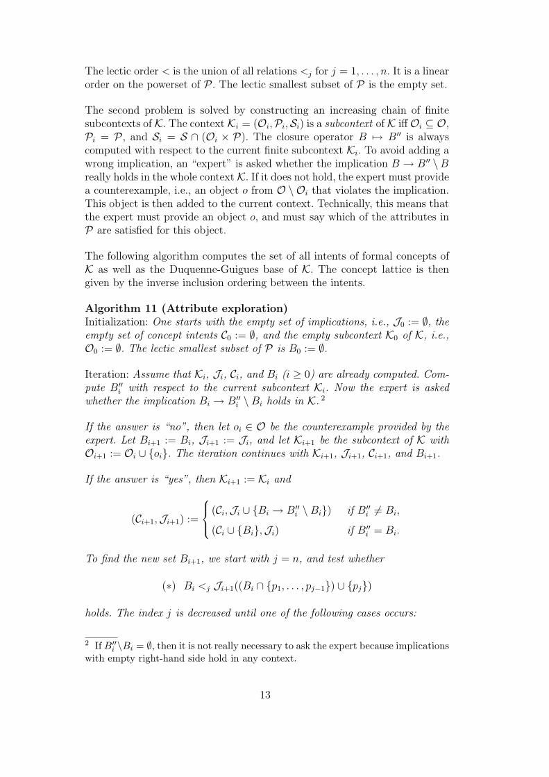
The lectic order < is the union of all relations <j for j = 1, . . . , n. It is a linearorder on the powerset of P . The lectic smallest subset of P is the empty set.

The second problem is solved by constructing an increasing chain of finitesubcontexts of K. The context Ki = (Oi,Pi,Si) is a subcontext of K iffOi ⊆ O,Pi = P , and Si = S ∩ (Oi × P). The closure operator B 7→ B′′ is alwayscomputed with respect to the current finite subcontext Ki. To avoid adding awrong implication, an “expert” is asked whether the implication B → B′′ \Breally holds in the whole context K. If it does not hold, the expert must providea counterexample, i.e., an object o from O \ Oi that violates the implication.This object is then added to the current context. Technically, this means thatthe expert must provide an object o, and must say which of the attributes inP are satisfied for this object.

The following algorithm computes the set of all intents of formal concepts ofK as well as the Duquenne-Guigues base of K. The concept lattice is thengiven by the inverse inclusion ordering between the intents.

Algorithm 11 (Attribute exploration)Initialization: One starts with the empty set of implications, i.e., J0 := ∅, theempty set of concept intents C0 := ∅, and the empty subcontext K0 of K, i.e.,O0 := ∅. The lectic smallest subset of P is B0 := ∅.

Iteration: Assume that Ki, Ji, Ci, and Bi (i ≥ 0) are already computed. Com-pute B′′

i with respect to the current subcontext Ki. Now the expert is askedwhether the implication Bi → B′′

i \Bi holds in K. 2

If the answer is “no”, then let oi ∈ O be the counterexample provided by theexpert. Let Bi+1 := Bi, Ji+1 := Ji, and let Ki+1 be the subcontext of K withOi+1 := Oi ∪ {oi}. The iteration continues with Ki+1, Ji+1, Ci+1, and Bi+1.

If the answer is “yes”, then Ki+1 := Ki and

(Ci+1,Ji+1) :=

(Ci,Ji ∪ {Bi → B′′i \Bi}) if B′′

i 6= Bi,

(Ci ∪ {Bi},Ji) if B′′i = Bi.

To find the new set Bi+1, we start with j = n, and test whether

(∗) Bi <j Ji+1((Bi ∩ {p1, . . . , pj−1}) ∪ {pj})

holds. The index j is decreased until one of the following cases occurs:

2 If B′′i \Bi = ∅, then it is not really necessary to ask the expert because implications

with empty right-hand side hold in any context.

13

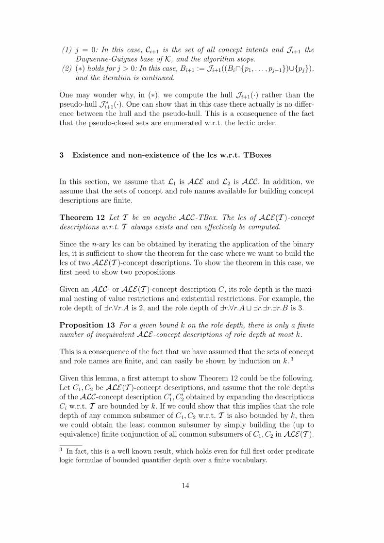
(1) j = 0: In this case, Ci+1 is the set of all concept intents and Ji+1 theDuquenne-Guigues base of K, and the algorithm stops.

(2) (∗) holds for j > 0: In this case, Bi+1 := Ji+1((Bi∩{p1, . . . , pj−1})∪{pj}),and the iteration is continued.

One may wonder why, in (∗), we compute the hull Ji+1(·) rather than thepseudo-hull J ∗

i+1(·). One can show that in this case there actually is no differ-ence between the hull and the pseudo-hull. This is a consequence of the factthat the pseudo-closed sets are enumerated w.r.t. the lectic order.

3 Existence and non-existence of the lcs w.r.t. TBoxes

In this section, we assume that L1 is ALE and L2 is ALC. In addition, weassume that the sets of concept and role names available for building conceptdescriptions are finite.

Theorem 12 Let T be an acyclic ALC-TBox. The lcs of ALE(T )-conceptdescriptions w.r.t. T always exists and can effectively be computed.

Since the n-ary lcs can be obtained by iterating the application of the binarylcs, it is sufficient to show the theorem for the case where we want to build thelcs of two ALE(T )-concept descriptions. To show the theorem in this case, wefirst need to show two propositions.

Given an ALC- or ALE(T )-concept description C, its role depth is the maxi-mal nesting of value restrictions and existential restrictions. For example, therole depth of ∃r.∀r.A is 2, and the role depth of ∃r.∀r.A t ∃r.∃r.∃r.B is 3.

Proposition 13 For a given bound k on the role depth, there is only a finitenumber of inequivalent ALE-concept descriptions of role depth at most k.

This is a consequence of the fact that we have assumed that the sets of conceptand role names are finite, and can easily be shown by induction on k. 3

Given this lemma, a first attempt to show Theorem 12 could be the following.Let C1, C2 be ALE(T )-concept descriptions, and assume that the role depthsof the ALC-concept description C ′

1, C′2 obtained by expanding the descriptions

Ci w.r.t. T are bounded by k. If we could show that this implies that the roledepth of any common subsumer of C1, C2 w.r.t. T is also bounded by k, thenwe could obtain the least common subsumer by simply building the (up toequivalence) finite conjunction of all common subsumers of C1, C2 in ALE(T ).

3 In fact, this is a well-known result, which holds even for full first-order predicatelogic formulae of bounded quantifier depth over a finite vocabulary.

14

However, due to the fact that in ALC and ALE we can define unsatisfiableconcepts, this simple approach does not work. In fact,⊥ has role depth 0, but itis subsumed by any concept description. Given this counterexample, the nextconjecture could be that it is enough to prevent this pathological case, i.e.,assume that at least one of the concept descriptions C1, C2 is satisfiable w.r.t.T , i.e., not subsumed by ⊥ w.r.t. T . This assumption can be made withoutloss of generality. In fact, if C1 is unsatisfiable w.r.t. T (i.e., equivalent to ⊥w.r.t. T ), then C2 is the lcs of C1, C2 w.r.t. T . For the DL EL in place of ALE ,this modification of the simple approach sketched above really works (see[50] for details). However, due to the presence of value restrictions, it does notwork for ALE . For example, ∀r.⊥ is subsumed by ∀r.F for arbitrary ALE(T )-concept descriptions F , and thus the role depth of common subsumers cannotbe bounded. However, we can show that common subsumers having a largerole depth are too general anyway.

Before giving a more formal statement of this result in Proposition 18, weshow some basic model-theoretic facts about ALE and ALC, which will beemployed in the proof of this proposition. An interpretation I is tree-shaped ifthe role relationships in I form a tree, i.e., if the directed graph GI = (VI , EI)with VI = ∆I and

EI = {(d, d′) | (d, d′) ∈ rI for some role r ∈ NR}

is a tree. An interpretation I is a tree-shaped counterexample to the subsump-tion question C v?

T D iff I is a tree-shaped model of T with root d0 ∈ CI\DI .

Lemma 14 Let T be an acyclic ALC-TBox and C, D ALC-concept descrip-tions. If C 6vT D, then the subsumption question C v?

T D has a tree-shapedcounterexample.

Proof. Assume that C 6vT D, and let C ′, D′ be the ALC-concept descrip-tions obtained by expanding C, D w.r.t. T . Then C ′ u ¬D′ is satisfiable. It iswell-known that the tableau-based satisfiability procedure for ALC [37] thenproduces a tree-shaped interpretation I whose root d0 satisfies d0 ∈ C ′I \D′I .Since C ′, D′ do not contain concept names defined in T , and since T is acyclic,we can assume without loss of generality that I is a model of T . In fact, oth-erwise we can modify I by setting AI := C ′I

A for all defined concepts A, whereA ≡ CA is the definition of A in T , and C ′

A is the expansion of CA w.r.t. T .

In case D = ⊥, the statement C 6vT D is equivalent to saying that C issatisfiable w.r.t. T , and thus the lemma also implies that any ALC-conceptdescription that is satisfiable w.r.t. T has a tree-shaped model, i.e., a tree-shaped model of T with root d0 ∈ CI . Of course, this and the above lemmaalso hold when the TBox is empty, i.e., for satisfiability and subsumption ofconcept descriptions.

15

Let I be a tree-shaped model of the acyclic ALC-TBox T , and C0 be an ALC-concept description. An element d of I is at level k if the unique path fromthe root d0 of I to d has length k. A subdescription F of C0 is at level k if itoccurs within k nestings of value and existential restrictions. For example, inthe description A u ∃r.(B t ∀r.C), the subdescription A occurs at level 0, Boccurs at level 1, and C occurs at level 2.

When evaluating C0 in I, i.e., when checking whether the root d0 of I belongsto CI

0 , we can directly use the inductive definition of the semantics of ALC-concept descriptions. During this evaluation process, one recursively checkswhether certain elements d of I belong to F I for subdescriptions F of C0. Itis easy to see that, in such a recursive test, the level of F in C0 always coincideswith the level of d in I. In particular, this means that elements of I that areat a level higher than the role depth of C0 are irrelevant when evaluating C0.The following lemma is an immediate consequence of this observation.

Lemma 15 Let C0 be an ALC-concept description of role depth `, and letI, I ′ be tree-shaped interpretations that differ from each other only on elementsat levels larger than `. Then d0 ∈ CI

0 iff d0 ∈ CI′0 , where d0 is the (common)

root of I and I ′.

In the proof of Proposition 18 we will need a specific result regarding the eval-uation of ALC-concept descriptions that are obtained by expanding ALE(T )-concept descriptions, where T is an acyclic ALC-TBox. Before we can formu-late this result in Lemma 17, we must introduce some more notation.

Let C0 be an ALC-concept description. We define under what conditions asubdescription F of C0 occurs conjunctively in C0 by induction on the level `of F in C0:

• if ` = 0, then C0 must be of the form F0 u F ; 4

• if ` > 0, then C0 must be of the form F0 u ∃r.C ′ or F0 u ∀r.C ′, where Foccurs conjunctively in C ′ on level `− 1. 5

The following lemma, which can easily be proved by induction on `, links thisnotion to ALE(T )-concept descriptions. Given an an acyclic ALC-TBox Tand an ALE(T )-concept description C0, the subdescription F of C0 is calledpositive if it is not a concept name that occurs within an atomic negation. Forexample, in the concept description C0 = ¬A u ∃r.¬B, the subdescriptions Aand B are not positive, but all other subdescriptions (e.g., ¬A or ∃r.¬B) arepositive.

4 The representation of C0 as F0 uF is meant modulo associativity and commuta-tivity of conjunction, and the fact that > is a unit for conjunction.5 Again, this representation of C0 should be read modulo associativity and com-mutativity of conjunction, and the fact that > is a unit for conjunction.

16

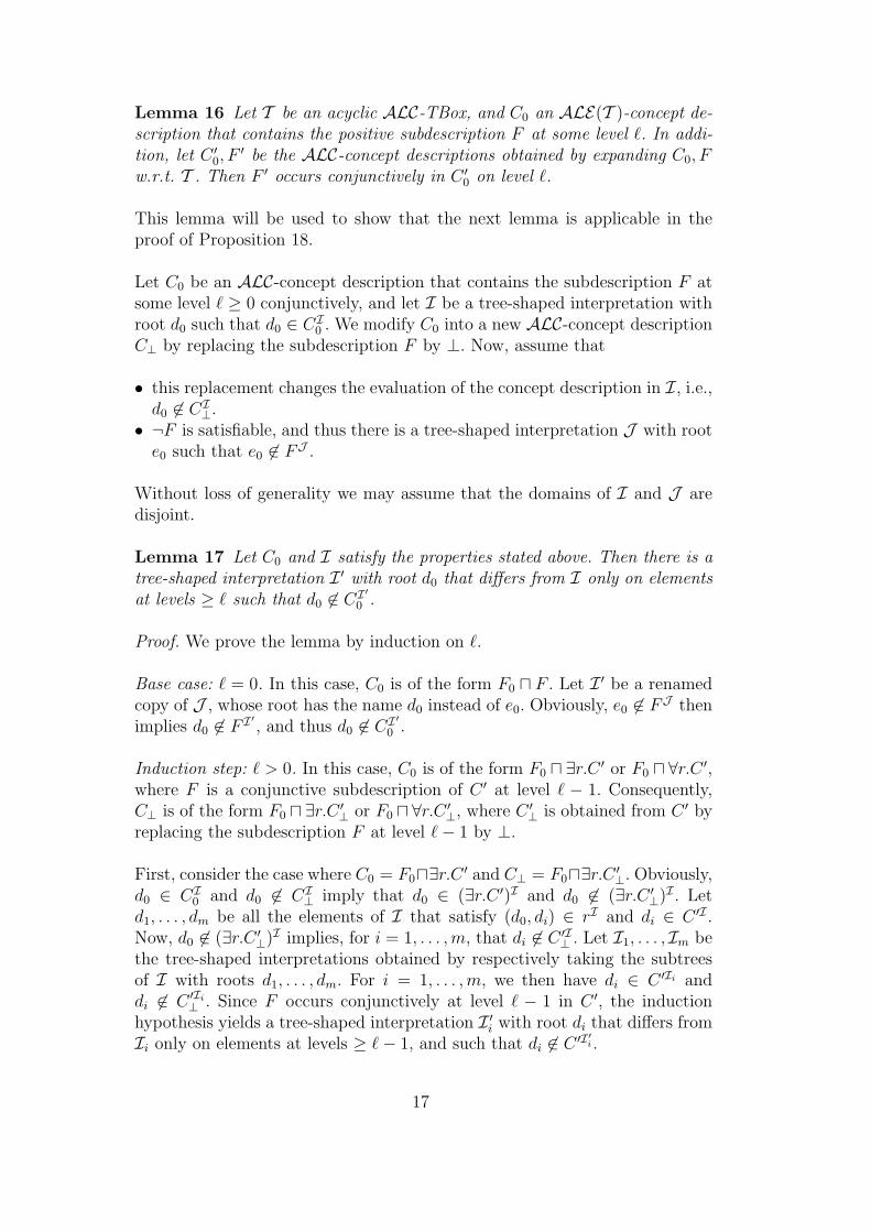
Lemma 16 Let T be an acyclic ALC-TBox, and C0 an ALE(T )-concept de-scription that contains the positive subdescription F at some level `. In addi-tion, let C ′

0, F′ be the ALC-concept descriptions obtained by expanding C0, F

w.r.t. T . Then F ′ occurs conjunctively in C ′0 on level `.

This lemma will be used to show that the next lemma is applicable in theproof of Proposition 18.

Let C0 be an ALC-concept description that contains the subdescription F atsome level ` ≥ 0 conjunctively, and let I be a tree-shaped interpretation withroot d0 such that d0 ∈ CI

0 . We modify C0 into a new ALC-concept descriptionC⊥ by replacing the subdescription F by ⊥. Now, assume that

• this replacement changes the evaluation of the concept description in I, i.e.,d0 6∈ CI

⊥.• ¬F is satisfiable, and thus there is a tree-shaped interpretation J with root

e0 such that e0 6∈ FJ .

Without loss of generality we may assume that the domains of I and J aredisjoint.

Lemma 17 Let C0 and I satisfy the properties stated above. Then there is atree-shaped interpretation I ′ with root d0 that differs from I only on elementsat levels ≥ ` such that d0 6∈ CI′

0 .

Proof. We prove the lemma by induction on `.

Base case: ` = 0. In this case, C0 is of the form F0 u F . Let I ′ be a renamedcopy of J , whose root has the name d0 instead of e0. Obviously, e0 6∈ FJ thenimplies d0 6∈ F I′ , and thus d0 6∈ CI′

0 .

Induction step: ` > 0. In this case, C0 is of the form F0 u ∃r.C ′ or F0 u ∀r.C ′,where F is a conjunctive subdescription of C ′ at level ` − 1. Consequently,C⊥ is of the form F0 u ∃r.C ′

⊥ or F0 u ∀r.C ′⊥, where C ′

⊥ is obtained from C ′ byreplacing the subdescription F at level `− 1 by ⊥.

First, consider the case where C0 = F0u∃r.C ′ and C⊥ = F0u∃r.C ′⊥. Obviously,

d0 ∈ CI0 and d0 6∈ CI

⊥ imply that d0 ∈ (∃r.C ′)I and d0 6∈ (∃r.C ′⊥)I . Let

d1, . . . , dm be all the elements of I that satisfy (d0, di) ∈ rI and di ∈ C ′I .Now, d0 6∈ (∃r.C ′

⊥)I implies, for i = 1, . . . ,m, that di 6∈ C ′I⊥ . Let I1, . . . , Im be

the tree-shaped interpretations obtained by respectively taking the subtreesof I with roots d1, . . . , dm. For i = 1, . . . ,m, we then have di ∈ C ′Ii anddi 6∈ C ′Ii

⊥ . Since F occurs conjunctively at level ` − 1 in C ′, the inductionhypothesis yields a tree-shaped interpretation I ′i with root di that differs fromIi only on elements at levels ≥ `− 1, and such that di 6∈ C ′I′i .

17

The interpretation I ′ is obtained from I be replacing, for i = 1, . . . ,m, thesubtree Ii with root di by I ′i. Obviously, I is tree-shaped and it differs fromI ′ only on elements at levels ≥ `. We claim that d0 6∈ (∃r.C ′)I

′, and thus

d0 6∈ CI′0 . In fact, let d be such that (d0, d) ∈ rI

′. By the definition of I ′, this

implies that (d0, d) ∈ rI . If d = di for some i, 1 ≤ i ≤ m, then d = di 6∈ C ′I′i ,and thus d = di 6∈ C ′I′ since the subtree with root di of I ′ coincides withI ′i. Otherwise, d 6∈ C ′I , and thus d 6∈ C ′I′ since I coincides with I ′ on therespective subtrees with root d.

Second, consider the case where C0 = F0 u ∀r.C ′ and C⊥ = F0 u ∀r.C ′⊥.

Obviously, d0 ∈ CI0 and d0 6∈ CI

⊥ imply that d0 ∈ (∀r.C ′)I and d0 6∈ (∀r.C ′⊥)I .

Let d1, . . . , dm be all the elements of I that satisfy (d0, di) ∈ rI . Now, d0 ∈(∀r.C ′)I implies di ∈ C ′I for all i, 1 ≤ i ≤ m. In addition, d0 6∈ (∀r.C ′

⊥)I

implies that there exists a j, 1 ≤ j ≤ m, such that dj 6∈ C ′I⊥ . Let Ij be the

tree-shaped interpretation obtained by taking the subtree of I with root dj.

Then, we have dj ∈ C ′Ij and dj 6∈ C′Ij

⊥ . Since F occurs conjunctively at level` − 1 in C ′, the induction hypothesis yields a tree-shaped interpretation I ′jwith root dj that differs from Ij only on elements at levels ≥ `− 1, and such

that dj 6∈ C ′I′j .

The interpretation I ′ is obtained from I be replacing the subtree Ij with rootdj by I ′j. Obviously, I is tree-shaped and it differs from I ′ only on elements

at levels ≥ `. We claim that d0 6∈ (∀r.C ′)I′, and thus d0 6∈ CI′

0 . This is animmediate consequence of the following two facts: (i) (d0, dj) ∈ rI

′, and (ii)

dj 6∈ C ′I′j , and thus dj 6∈ C ′I′ since the subtree with root dj of I ′ coincideswith I ′j.

We are now ready to prove the key proposition.

Proposition 18 Let C1, C2 be ALE(T )-concept descriptions that are bothsatisfiable w.r.t. T , and assume that the role depths of the ALC-concept de-scriptions C ′

1, C′2 obtained by expanding the descriptions C1, C2 w.r.t. T are

bounded by k. If the ALE(T )-concept description D is a common subsumerof C1, C2 w.r.t. T , then there is an ALE(T )-concept description D0 vT D ofrole depth at most k + 1 that is also a common subsumer of C1, C2 w.r.t. T .

Proof. Let D be an ALE(T )-concept description that is a common subsumerof C1, C2 w.r.t. T . If the role depth of D is bounded by k+1, then we are donesince we can take D0 = D. Otherwise, D contains at least one subdescriptionon level k+1 that is an existential or a value restriction. Choose such a subde-scription F . Obviously, F is positive. We modify D into a concept descriptionD as follows. We replace F by either > or ⊥:

• if F is equivalent to > w.r.t. T , then it is replaced by >;• otherwise, F is replaced by ⊥.

18

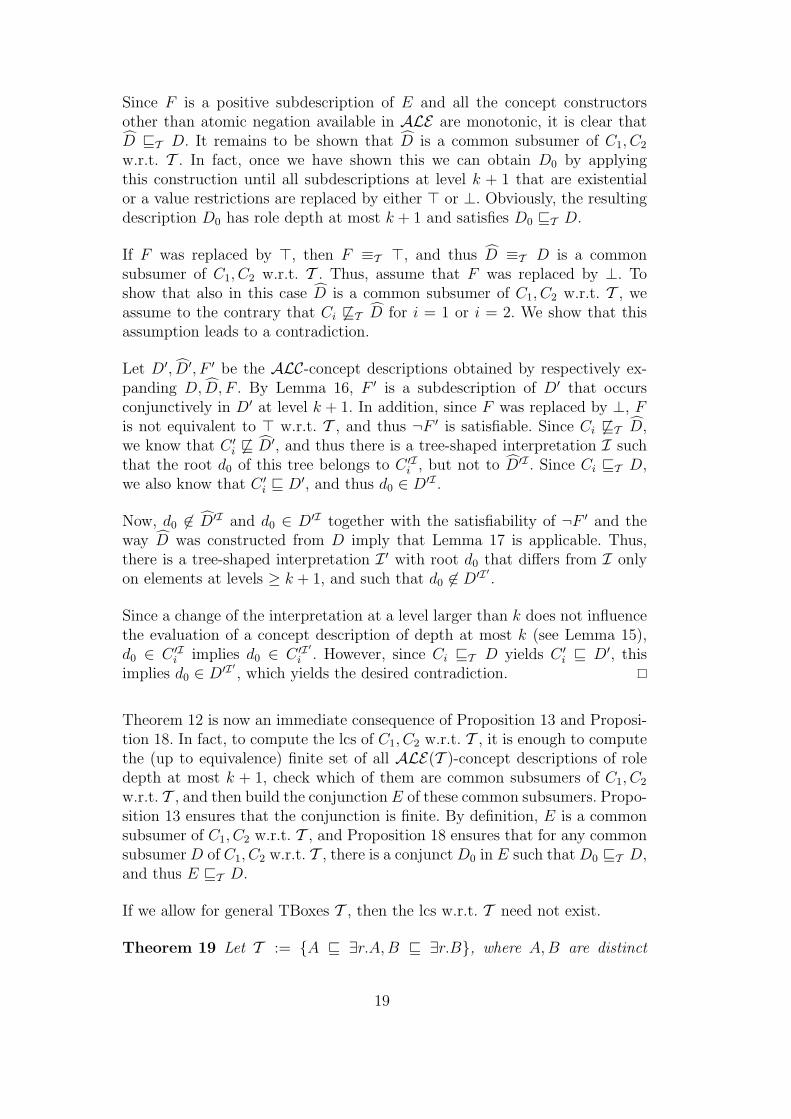
Since F is a positive subdescription of E and all the concept constructorsother than atomic negation available in ALE are monotonic, it is clear thatD vT D. It remains to be shown that D is a common subsumer of C1, C2

w.r.t. T . In fact, once we have shown this we can obtain D0 by applyingthis construction until all subdescriptions at level k + 1 that are existentialor a value restrictions are replaced by either > or ⊥. Obviously, the resultingdescription D0 has role depth at most k + 1 and satisfies D0 vT D.

If F was replaced by >, then F ≡T >, and thus D ≡T D is a commonsubsumer of C1, C2 w.r.t. T . Thus, assume that F was replaced by ⊥. Toshow that also in this case D is a common subsumer of C1, C2 w.r.t. T , weassume to the contrary that Ci 6vT D for i = 1 or i = 2. We show that thisassumption leads to a contradiction.

Let D′, D′, F ′ be the ALC-concept descriptions obtained by respectively ex-panding D, D, F . By Lemma 16, F ′ is a subdescription of D′ that occursconjunctively in D′ at level k + 1. In addition, since F was replaced by ⊥, Fis not equivalent to > w.r.t. T , and thus ¬F ′ is satisfiable. Since Ci 6vT D,we know that C ′

i 6v D′, and thus there is a tree-shaped interpretation I suchthat the root d0 of this tree belongs to C ′I

i , but not to D′I . Since Ci vT D,we also know that C ′

i v D′, and thus d0 ∈ D′I .

Now, d0 6∈ D′I and d0 ∈ D′I together with the satisfiability of ¬F ′ and theway D was constructed from D imply that Lemma 17 is applicable. Thus,there is a tree-shaped interpretation I ′ with root d0 that differs from I onlyon elements at levels ≥ k + 1, and such that d0 6∈ D′I′ .

Since a change of the interpretation at a level larger than k does not influencethe evaluation of a concept description of depth at most k (see Lemma 15),d0 ∈ C ′I

i implies d0 ∈ C ′I′i . However, since Ci vT D yields C ′

i v D′, thisimplies d0 ∈ D′I′ , which yields the desired contradiction.

Theorem 12 is now an immediate consequence of Proposition 13 and Proposi-tion 18. In fact, to compute the lcs of C1, C2 w.r.t. T , it is enough to computethe (up to equivalence) finite set of all ALE(T )-concept descriptions of roledepth at most k + 1, check which of them are common subsumers of C1, C2

w.r.t. T , and then build the conjunction E of these common subsumers. Propo-sition 13 ensures that the conjunction is finite. By definition, E is a commonsubsumer of C1, C2 w.r.t. T , and Proposition 18 ensures that for any commonsubsumer D of C1, C2 w.r.t. T , there is a conjunct D0 in E such that D0 vT D,and thus E vT D.

If we allow for general TBoxes T , then the lcs w.r.t. T need not exist.

Theorem 19 Let T := {A v ∃r.A, B v ∃r.B}, where A, B are distinct

19

concept names. Then, the lcs of the ALE(T )-concept descriptions A, B w.r.t.T does not exist.

Proof. Consider a common subsumer E of A, B w.r.t. T . Without loss of gen-erality we can assume that the ALE(T )-concept description E is a conjunctionof (negated) concept names, value restrictions, and existential restrictions. Weclaim that this conjunction can actually only contain existential restrictionsfor the role r.

Assume that the concept name P is contained in this conjunction. We restrictour attention to the case where P is different from A (otherwise, P is differentfrom B, and we can proceed analogously). Consider the interpretation I thatconsists of one element a, which belongs to A and to no other concept name,and which is related to itself via the role r. Then I is a model of T , anda ∈ AI . However, a 6∈ P I , which is a contradiction since P occurs in thetop-level conjunction of E, and we have assumed that A vT E. Similarly, wecan show that no negated concept name can occur in this conjunction.

For similar reasons, the conjunction cannot contain a value restriction ∀s.Fwhere F is not equivalent to > w.r.t. T . 6 In fact, if F is not equivalent to> w.r.t. T , then there is a model I¬F of T that contains an element d0 withd0 6∈ F I¬F . We extend I¬F to an interpretation I by adding a new elementa, which belongs to A and to no other concept name, and which is related toitself via the role r, and to d0 via the role s. Then I is a model of T , anda ∈ AI . However, a 6∈ (∀s.F )I , which is a contradiction since A vT E.

Thus, we may assume without loss of generality that both the conjunction of(negated) concept names and the conjunction of value restrictions is empty.Now, consider an existential restriction ∃s.F . By using a construction similarto the ones above, we can show that s must in fact be equal to r, i.e., we havean existential restriction of the form ∃r.F . We claim that F is again a commonsubsumer of A, B w.r.t. T . Otherwise, we assume without loss of generalitythat A 6vT F , i.e., there is a model I0 of T that contains an element d0 suchthat d0 ∈ AI0 \ F I0 . This is a contradiction to A vT E vT ∃r.F since usingI0 we can easily construct a model I of T that contains an element a thatbelongs to A, but not to ∃r.F . In fact, I is obtained from I0 by adding a newelement a, which belongs to A and to no other concept name, and which isrelated to d0 via the role r.

We can now apply induction over the role depth of the common subsumer Eof A, B to show that E is equivalent w.r.t. T to an ALE-concept descriptionfrom the following set of descriptions: S is the smallest set of ALE-conceptdescriptions such that

6 If F is equivalent to >, then ∀s.F is equivalent to >, and thus it can be removed.

20

• > belongs to S;• S is closed under conjunction;• if F belongs to S, then ∃r.F also belongs to S.

Conversely, it is easy to show (by induction on the size of elements of S) thatany element of S is a common subsumer of A, B w.r.t. T .

Thus, a least common subsumer of A, B w.r.t. T must be a least element of S.Since the elements of S do not contain A, B, least is meant w.r.t. subsumptionof concept descriptions (i.e., without a TBox). However, S does not have a leastelement w.r.t. subsumption. On the one hand, S obviously contains elementsof arbitrary role depth. On the other hand, an element D of role depth `cannot be subsumed by an element E of role depth k > `: if d ∈ EI forsome interpretation I and element d of I, then there is a path of length kstarting from d in the graph GI ; in contrast, there is an interpretation I0 andan element d0 of I0 such that d0 ∈ DI0 , but all paths in GI0 starting with d0

have length ≤ ` < k.

It is easy to see that the same proof also works for the cyclic TBox T := {A ≡∃r.A, B ≡ ∃r.B}.

Corollary 20 Let T := {A ≡ ∃r.A, B ≡ ∃r.B}, where A, B are distinctconcept names. Then, the lcs of the ALE(T )-concept descriptions A, B w.r.t.T does not exist.

4 Good common subsumers

The brute-force algorithm for computing the lcs in ALE(T ) w.r.t. an acyclicbackground ALC-TBox described in the previous section is not useful in prac-tice since the number of concept descriptions that must be considered is verylarge (super-exponential in the role depth). In addition, w.r.t. cyclic or generalTBoxes the lcs need not exist. In the bottom-up construction of DL knowl-edge bases, it is not really necessary to take the least common subsumer, 7 acommon subsumer that is not too general can also be used. In this section, weintroduce an approach for computing such “good” common subsumers w.r.t.a background TBox. In order to explain this approach, we must first recallhow the lcs of ALE-concept descriptions (without background TBox) can becomputed.

7 Using it may even result in over-fitting.

21

4.1 The lcs of ALE-concept descriptions

Since the lcs of n concept descriptions can be obtained by iterating the applica-tion of the binary lcs, we describe how to compute the least common subsumerlcsALE(C, D) of two ALE-concept descriptions C, D (see [22] for more detailsand a proof of correctness).

First, the input descriptions C, D are normalized by applying the followingequivalence-preserving rules modulo associativity and commutativity of con-junction:

∀r.E u ∀r.F −→ ∀r.(E u F ), ∀r.E u ∃r.F −→ ∀r.E u ∃r.(E u F ),

∀r.> −→ >, E u > −→ E,

∃r.⊥ −→ ⊥, E u ⊥ −→ ⊥,

A u ¬A −→ ⊥ for each A ∈ NC .

Note that, due to the second rule in the first line, this normalization may leadto an exponential blow-up of the concept descriptions. In the following, weassume that the input descriptions C, D are normalized.

In order to describe the lcs algorithm, we need to introduce some notation.Let C be a normalized ALE-concept description. Then names(C) (names(C))denotes the set of (negated) concept names occurring in the top-level conjunc-tion of C, roles∃(C) (roles∀(C)) the set of role names occurring in an existential(value) restriction on the top-level of C, and restrict∃r (C) (restrict∀r (C)) denotesthe set of all concept descriptions occurring in an existential (value) restrictionon the role r in the top-level conjunction of C.

Now, let C, D be normalized ALE-concept descriptions. If C (D) is equivalentto ⊥, then lcsALE(C, D) = D (lcsALE(C, D) = C). Otherwise, we have

lcsALE(C, D) = uA∈names(C)∩names(D)

A u u¬B∈names(C)∩names(D)

¬B u

ur∈roles∃(C)∩roles∃(D)

uE∈restrict∃r (C),F∈restrict∃r (D)

∃r.lcsALE(E, F ) u

ur∈roles∀(C)∩roles∀(D)

uE∈restrict∀r (C),F∈restrict∀r (D)

∀r.lcsALE(E, F ).

Here, the empty conjunction stands for the top-concept >. The recursive callsof lcsALE are well-founded since the role depth decreases with each call.

22

4.2 A good common subsumer in ALE w.r.t. a background TBox

Let T be a background TBox in some DL L2 extending ALE such that sub-sumption in L2 w.r.t. this kind of TBoxes is decidable. 8 Let C, D be normal-ized ALE(T )-concept descriptions. If we ignore the TBox, then we can simplyapply the above algorithm for ALE-concept descriptions without backgroundterminology to compute a common subsumer. However, in this context, taking

uA∈names(C)∩names(D)

A u u¬B∈names(C)∩names(D)

¬B

is not the best we can do. In fact, some of these concept names may beconstrained by the TBox, and thus there may be relationships between themthat we ignore by simply using the intersection. Instead, we propose to takethe smallest (w.r.t. subsumption w.r.t. T ) conjunction of concept names andnegated concept names that subsumes (w.r.t. T ) both

uA∈names(C)

A u u¬B∈names(C)

¬B and uA′∈names(D)

A′ u u¬B′∈names(D)

¬B′.

We modify the above lcs algorithm in this way, not only on the top-level ofthe input concepts, but also in the recursive steps. It is easy to show that theALE(T )-concept description computed by this modified algorithm still is acommon subsumer of A, B w.r.t. T .

Proposition 21 The ALE(T )-concept description E obtained by applying themodified lcs algorithm to ALE(T )-concept descriptions C, D is a common sub-sumer of C and D w.r.t. T , i.e., C vT E and D vT E.

In general, this common subsumer will be more specific than the one obtainedby ignoring T , though it need not be the least common subsumer. In thefollowing, we will call the common subsumer computed this way good commonsubsumer (gcs), and the algorithm that computes it the gcs algorithm.

Example 22 As a simple example, consider the ALC-TBox T :

NoSon ≡ ∀has-child.Female,

NoDaughter ≡ ∀has-child.¬Female,

SonRichDoctor ≡ ∀has-child.(Female t (Doctor u Rich)),

DaughterHappyDoctor ≡ ∀has-child.(¬Female t (Doctor u Happy)),

ChildrenDoctor ≡ ∀has-child.Doctor,

8 Note that the TBox T used as background terminology may be a general TBox.

23

and the ALE-concept descriptions

C := ∃has-child.(NoSon u DaughterHappyDoctor),

D := ∃has-child.(NoDaughter u SonRichDoctor).

By ignoring the TBox, we obtain theALE(T )-concept description ∃has-child.>as common subsumer of C, D. However, if we take into account that bothNoSonuDaughterHappyDoctor and NoDaughteruSonRichDoctor are subsumedby the concept ChildrenDoctor, then we obtain the more specific commonsubsumer ∃has-child.ChildrenDoctor. The gcs of C, D is even more specific.In fact, the least conjunction of (negated) concept names subsuming bothNoSon u DaughterHappyDoctor and NoDaughter u SonRichDoctor is

ChildrenDoctor u DaughterHappyDoctor u SonRichDoctor,

and thus the gcs of C, D is

∃has-child.(ChildrenDoctor u DaughterHappyDoctor u SonRichDoctor).

The conjunct ChildrenDoctor is actually redundant since it is implied by theremainder of the conjunction.

In order to implement the gcs algorithm, we must be able to compute thesmallest conjunction of (negated) concept names that subsumes two such con-junctions C1 and C2 w.r.t. T . In principle, one can compute this smallest con-junction by testing, for every (negated) concept name whether it subsumesboth C1 and C2 w.r.t. T , and then take the conjunction of those (negated)concept names for which the test was positive. However, this results in alarge number of (possibly quite expensive) calls to the subsumption algorithmfor L2 w.r.t. (general or (a)cyclic) TBoxes. Since in our application scenario(bottom-up construction of DL knowledge bases w.r.t. a given background ter-minology), the TBox T is assumed to be fixed, it makes sense to precomputethis information. In Section 5 we will show that attribute exploration can beused for this purpose.

4.3 Using ALE-expansion when computing the gcs

If the background terminology is an acyclic TBox T , then one can employan appropriate partial expansion of T in order to uncover ALE-parts hiddenwithin the defined concepts. The idea is that the gcs algorithm will possiblyyield a more specific common subsumer if it can make use of ALE-concepts“hidden” within the defined concepts.

24

For instance, in Example 22, the concepts defining NoSon and NoDaughter areactually ALE(T )-concept descriptions, and thus C, D can be expanded to

C ′ := ∃has-child.(∀has-child.Female u DaughterHappyDoctor),

D′ := ∃has-child.(∀has-child.¬Female u SonRichDoctor),

before computing the gcs. The concepts defining DaughterHappyDoctor andSonRichDoctor are notALE(T )-concept descriptions, and thus these two namescannot be expanded. However, in this example, the common subsumer com-puted by applying the gcs algorithm to the expanded concepts C ′, D′ is

∃has-child.>,

which is actually less specific than the result of applying the gcs algorithm tothe unexpanded concepts C, D. To overcome this problem, we do the partialexpansion, but also keep the defined concepts that we have expanded. In theexample, this yields the expanded concepts

C ′′ := ∃has-child.(∀has-child.Female u NoSon u DaughterHappyDoctor),

D′′ := ∃has-child.(∀has-child.¬Female u NoDaughter u SonRichDoctor).

If we apply the gcs algorithm to C ′′, D′′, then we obtain (up to equivalencew.r.t. T ) the same common subsumer as obtained from C, D, i.e., in this casethe expansion does not yield a more specific result.

However, it is easy to construct examples where this kind of expansion leads tobetter results. For instance, if we apply the gcs algorithm to ∀has-child.(FemaleuDoctor) and NoSon u ∀has-child.Happy, then the result is >. In contrast, if weapply it to the expanded concept descriptions ∀has-child.(Female u Doctor)and NoSon u ∀has-child.Female u ∀has-child.Happy, then the result is the morespecific common subsumer ∀has-child.Female.

Before checking whether a defined concept can be expanded, it is useful totransform it into negation normal form (NNF) by pushing all negations intothe description until they occur only in front of concept names, using deMorgan’ rules and the facts that ¬¬D ≡ D and ¬> ≡ ⊥. For example, theconcept description ¬∀has-child.Female is not anALE-concept description, butits negation normal form ∃has-child.¬Female is.

More formally, we define the ALE-expansion of (negated) concept names de-fined in T and of ALE(T )-concept descriptions as follows.

Definition 23 (ALE-expansion) Let T be an acyclic TBox, let A be a con-cept name defined in T , and let A ≡ C be its definition. We first build thenegation normal form C ′ of C. If C ′ is not an ALE(T )-concept description,

25

then the ALE-expansion of A is A. Otherwise, it is A u C ′′, where C ′′ isobtained from C ′ by replacing all (negated) defined concept names in C ′ bytheir ALE-expansion. To obtain the ALE-expansion of ¬A, we just apply thesame approach to ¬C. The ALE-expansion of an ALE(T )-concept descriptionis obtained by replacing all (negated) defined concept names by their ALE-expansions.

Note that this recursive definition of an ALE-expansion is well-founded sincethe TBox is assumed to be acyclic. As an example, consider the TBox Tconsisting of

A ≡ ¬∀r.(B1 tB2), B1 ≡ P tQ, B2 ≡ P uQ.

Then we obtain A u ∃r.(¬B1 u ¬P u ¬Q u ¬B2) as ALE-expansion of A.

It is easy to see that ALE-expansion may lead to more specific common sub-sumers, but never to less specific ones.

Proposition 24 Let T be an acyclic L2-TBox, C, D ALE(T )-concept de-scriptions with ALE-expansion C ′, D′, and let E (E ′) be the result of applyingthe gcs algorithm to C, D (C ′, D′). Then E ′ is a common subsumer of C, Dthat is at least as good as E, i.e., C vT E ′, D vT E ′, and E ′ vT E.

ALE-expansion can also be applied to cyclic L2-TBoxes, provided that thecycles go through non-ALE parts of the TBox. This is, for example, the casein the TBox T := {A ≡ ∃r.B, B ≡ P t A}.

4.4 Alternative approaches for computing common subsumers

In Section 2.1 we have already sketched an approach based on approximation,which works if the TBox T is acyclic, L2 allows for disjunction, and onecan compute the approximation from above of L2-concept descriptions byALE-concept descriptions. For example, if we take ALC as L2, then all theseconditions are satisfied.

Definition 25 (Common subsumer by approximation) Assume that L2

allows for disjunction, and that one can compute the approximation from aboveof L2-concept descriptions by ALE-concept descriptions. Let T be an acyclicL2-TBox. Given ALE(T )-concept descriptions C, D, one first fully expandsthem into L2-concept descriptions C ′, D′. Then one approximates their dis-junction C ′ t D′ from above by an ALE-concept description. The commonsubsumer of C, D obtained this way is called the common subsumer by ap-proximation (acs) of C, D w.r.t. T .

26

In Section 2.1, we have shown by an example that the acs can be less specificthan the lcs. In this example (Example 4), the gcs coincides with the lcs, andthus is also more specific than the acs: in fact, w.r.t. the TBox T = {A ≡P tQ}, the smallest conjunction of concept names above both P and Q is A,and thus the gcs of P and Q is A.

There are, however, also examples where the gcs is less specific than the acs.For instance, consider the TBox

T = {A ≡ ∃r.A1 t ∃r.A2, B ≡ ∃r.B1 t ∃r.B2}.

With respect to this TBox, the gcs of A, B is >, whereas the acs is the morespecific common subsumer ∃r.>.

The gcs algorithm makes use of the subsumption relationships between con-junctions of (negated) concept names. Usually, these relationships are notknown for a given TBox, and thus we must either precompute them (seeSection 5) or compute them on the fly (as sketched in Section 4.2). Bothmay be quite expensive. What is usually known for a given TBox T are allsubsumption relationships between the concept names occurring in T . 9 Thisinformation can be used as follows. Given two conjunctions

uA∈names(C)

A u u¬B∈names(C)

¬B and uA′∈names(D)

A′ u u¬B′∈names(D)

¬B′,

the gcs algorithm takes the smallest (w.r.t. subsumption w.r.t. T ) conjunctionof concept names and negated concept names that subsumes (w.r.t. T ) bothconjunctions. In contrast, the algorithm that just ignores the TBox would take

uA∈names(C)∩names(D)

A u u¬B∈names(C)∩names(D)

¬B.

Using the subsumption relationships between concept names, we can come upwith a new approach that lies between these two approaches.

Definition 26 (Subsumption closure) Let T be a TBox, and S (S) a setof (negated) concept names. The subsumption closure of S (S) w.r.t. T is aset of (negated) concept names, which is defined as follows:

SC(S) := {A | ∃B ∈ S. B vT A},

SC(S) := {¬A | ∃¬B ∈ S. A vT B}.

Instead of using the intersection names(C)∩names(D) (names(C)∩names(D)),as in the approach that ignores T , one can first build the subsumption closures,

9 Most DL system compute these automatically when reading in a TBox.

27

and then intersect the closures, i.e., use

uA∈SC(names(C))∩SC(names(D))

A u u¬B∈SC(names(C))∩SC(names(D))

¬B.

We call the algorithm for computing common subsumers obtained this way thescs algorithm, and the result of applying it to ALE(T )-concept descriptionsC, D the scs of C, D w.r.t. T .

Proposition 27 Let T be an L2-TBox, C, D ALE(T )-concept descriptions,and let E (E ′) be the result of applying the gcs (scs) algorithm to C, D. ThenE ′ is a common subsumer of C, D that is at most as good as the gcs E, i.e.,C vT E ′, D vT E ′, and E vT E ′.

5 Computing the subsumption lattice of conjunctions of (negated)concept names w.r.t. a TBox

To obtain a practical gcs algorithm, we must be able to compute in an effi-cient way the smallest conjunction of (negated) concept names that subsumestwo such conjunctions w.r.t. T . Since in our application scenario (bottom-upconstruction of DL knowledge bases w.r.t. a given background terminology),the TBox T is assumed to be fixed, it makes sense to precompute this in-formation. Obviously, a naıve approach that calls the subsumption algorithmfor each pair of conjunctions of (negated) concept names is too expensive forTBoxes of a realistic size. Instead, we propose to use attribute exploration forthis purpose.

In order to apply attribute exploration to the task of computing the subsump-tion lattice 10 of conjunctions of (negated) concept names (some of which maybe defined concepts in an L2-TBox T ), we define a formal context whoseconcept lattice is isomorphic to the subsumption lattice we are interested in.

For the case of conjunctions of concept names (without negated names), thisproblem was first addressed in [51], where the objects of the context were basi-cally all possible counterexamples to subsumption relationships, i.e., interpre-tations together with an element of the interpretation domain. The resulting“semantic context” has the disadvantage that an “expert” for this contextmust be able to deliver such counterexamples, i.e., it is not sufficient to havea simple subsumption algorithm for the DL in question. One needs one that,given a subsumption problem “C v D?”, is able to compute a counterexample

10 In general, the subsumption relation induces a partial order, and not a latticestructure on concepts. However, in the case of conjunctions of (negated) conceptnames, all infima exist, and thus also all suprema.

28

if the subsumption relationship does not hold, i.e., an interpretation I and anelement d of its domain such that d ∈ CI \DI . Since the usual tableau-basedsubsumption algorithms [52] in principle try to generate finite countermodelsto subsumption relationships, they can usually be extended such that theyyield such an object in case the subsumption relationship does not hold. Forinstance, in [51], this is explicitly shown for the DL ALC. However, the highlyoptimized algorithms in systems like FaCT and Racer do not produce suchcountermodels as output. For this reason, we are interested in a context thathas the same attributes and the same concept lattice (up to isomorphism),but for which a standard subsumption algorithm can function as an expert.Such a context was first introduced in [53]:

Definition 28 Let T be an L2-TBox. The context KT = (O,P ,S) is definedas follows:

O := {E | E is an L2-concept description},P := {A1, . . . , An} is the set of concept names occurring in T ,

S := {(E, A) | E vT A}.

Before we can prove that this context has the desired properties, it is useful toshow the following lemma, which relates subsumption in T with implicationsholding in KT . If B is a set of attributes of KT (i.e., a set of concept names

occurring in T ), then uB denotes their conjunction, i.e., uB := uA∈B

A.

Lemma 29 Let B1, B2 be subsets of P. The implication B1 → B2 holds inKT iff uB1 vT uB2.

Proof. First, we prove the only if direction. If the implication B1 → B2 holdsin KT , then this means that the following holds for all objects E ∈ O: ifE vT p holds for all p ∈ B1, then E vT p also holds for all p ∈ B2. Thus,if we take uB1 as object E, we obviously have uB1 vT p for all p ∈ B1, andthus uB1 vT p for all p ∈ B2, which shows uB1 vT uB2.

Second, we prove the if direction. If uB1 vT uB2, then any object E satisfyingE vT uB1 also satisfies E vT uB2 by the transitivity of the subsumptionrelation. Consequently, if E is subsumed by all concepts in B1, then it is alsosubsumed by all concepts in B2, i.e., if E satisfies all attributes in B1, it alsosatisfies all attributes in B2. This shows that the implication B1 → B2 holdsin KT .

Given this lemma, we can now prove the main theorem of this section:

Theorem 30 The concept lattice of the context KT is isomorphic to the sub-

29

sumption hierarchy of all conjunctions of subsets of P w.r.t. T .

Proof. In order to obtain an appropriate isomorphism, we define a mappingπ from the formal concepts of the context KT to the set of all (equivalenceclasses of) conjunctions of subsets of P as follows:

π(A, B) = [uB]≡.

For formal concepts (A1, B1), (A2, B2) of KT we have (A1, B1) ≤ (A2, B2) iffB2 ⊆ B1. Since B1 is the intent of the formal concept (A1, B1), we have B1 =A′

1 = A′′′1 = B′′

1 , and thus B2 ⊆ B1 iff B2 ⊆ B′′1 iff the implication B1 → B2

holds in KT iff uB1 vT uB2. Overall, we have thus shown that π is an orderembedding (and thus injective): (A1, B1) ≤ (A2, B2) iff [uB1]≡ v≡

T [uB2]≡.

It remains to be shown that π is surjective as well. Let B be an arbitrarysubset of P . We must show that [uB]≡ can be obtained as an image underthe mapping π. We know that (B′, B′′) is a formal concept of KT , and thus itis sufficient to show that π(B′, B′′) = [uB]≡, i.e., u(B′′) ≡T uB. Obviously,B ⊆ B′′ implies u(B′′) vT uB. Conversely, the implication B → B′′ holds inKT , and thus Lemma 29 yields uB vT uB′′.

Attribute exploration can be used to compute the concept lattice of KT sinceany standard subsumption algorithm for the DL under consideration is anexpert for KT .

Proposition 31 Any decision procedure for subsumption w.r.t. TBoxes in L2

functions as an expert for the context KT .

Proof. The attribute exploration algorithm asks questions of the form “B1 →B2?” By Lemma 29, we can translate these questions into subsumption ques-tions of the form “uB1 vT uB2?” Obviously, any decision procedure for sub-sumption can answer these questions correctly.

Now, assume that B1 → B2 does not hold in KT , i.e., uB1 6vT uB2. Weclaim that uB1 is a counterexample, i.e., uB1 ∈ B′

1, but uB1 /∈ B′2. This is

an immediate consequence of the facts that B′i = {E | E vT uBi} (i = 1, 2)

and that uB1 vT uB1 and uB1 6vT uB2.

The expert must provide for each counterexample the information which at-tributes it satisfies and which it does not. This can again be realized by thesubsumption algorithm: uB1 satisfies the attribute Ai iff uB1 vT Ai.

In order to compute the gcs, we consider not only conjunctions of conceptnames, but rather conjunctions of concept names and negated concept names.The above results can easily be adapted to this case. In fact, one can simply

30

extend the TBox T by a definition for each negated concept name, and thenapply the approach to this extended TBox. To be more precise, if {A1, . . . , An}is the set of concept names occurring in T , then we introduce new conceptnames A1, . . . , An, and extend T to a TBox T by adding the definitions A1 ≡¬A1, . . . , An ≡ ¬An. 11

Corollary 32 The concept lattice of the context KT is isomorphic to the sub-sumption hierarchy of all conjunctions of concept names and negated conceptnames occurring in T .

How can this result be used to support computing the gcs? The above corollarytogether with Proposition 31 shows that attribute exploration applied to KTcan be used to compute the Duquenne-Guigues base of KT . Given this base,we can compute the supremum in the concept lattice of KT as follows:

Lemma 33 Let J be the Duquenne-Guigues base of KT , and let B1, B2 besets of attributes of KT . Then J (B1) ∩ J (B2) is the intent of the supremumof the formal concepts (B′

1, B′′1 ) and (B′

2, B′′2 ).

Proof. We know that the intent of the supremum of the formal concepts(B′

1, B′′1 ) and (B′

2, B′′2 ) is just the intersection B′′

1 ∩ B′′2 of their intents. In

addition, since Cons(J ) = Imp(KT ), we know that B′′i = J (Bi) for i = 1, 2.

As an immediate consequence of this lemma together with Theorem 30 andits proof, the supremum in the hierarchy of all conjunctions of concept namesand negated concept names occurring in T can be computed as follows:

Proposition 34 Let J be the Duquenne-Guigues base of KT , and let B1, B2

be sets of (negated) concept names occurring in T . Then

uL∈J (B1)∩J (B2)

L

is the least conjunction of (negated) concept names occurring in T that lies

above both uL∈B1

L and uL∈B2

L.

As mentioned in Section 2.2, computing the implication hull J (B) for a set ofattributes B can be done in time linear in the size of J and B. This means thatthe supremum can be computed efficiently as long as the Duquenne-Guiguesbase of KT is relatively small.

The experimental results reported in [53] show that using attribute explo-ration for computing the subsumption lattice of all conjunctions of (negated)

11 For T to be an L2-TBox, we must assume that L2 allows for full negation.

31

concept names gives a huge increase of efficiency compared to the semi-naıveapproach, which introduces a new definition for each of the exponentiallymany such conjunctions, and then applies the usual algorithm for comput-ing the subsumption hierarchy. Nevertheless, these results also show that theapproach can only be applied if the number of concept names is relativelysmall. Although these experiments were done almost 10 years ago on a ratherslow computer, using randomly generated TBoxes and the semantic context,our more recent experiments (see Section 6) come to a similar result. For thisreason, we have also experimented with an improved algorithm for comput-ing concept lattices [33,34], which can employ additional knowledge that isreadily available in our case, but not used by the basic attribute explorationalgorithm.

Using attribute exploration with a priori knowledge

When starting the exploration process, all the basic attribute exploration al-gorithm knows about the context is the set of its attributes. It acquires all thenecessary knowledge about the context by asking the expert, which in our set-ting means: by calling the subsumption algorithm for L2. Since L2 is usuallyan expressive DL, the complexity of the subsumption problem is usually quitehigh, and thus asking the expert may be expensive. For this reason it makessense to employ approaches that can avoid some of these expensive calls ofthe subsumption algorithm.

In our application, we already have some a priori knowledge about relation-ships between attributes. In fact, we know that the attributes Ai and Ai standfor a concept and its negation. In addition, since the background TBox T isassumed to be an existing terminology, we can usually assume that the sub-sumption hierarchy between the concept names occurring in T has alreadybeen computed. This provides us with the following a priori knowledge aboutthe relationships between attributes:

(1) If Ai vT Aj holds, then we know on the FCA side that in the contextKT all objects satisfying the attribute Ai also satisfy the attribute Aj,i.e., the implication {Ai} → {Aj} holds in KT .

(2) Since Ai vT Aj implies ¬Aj vT ¬Ai, we also know that all objects sat-isfying the attribute Aj also satisfy the attribute Ai, i.e., the implication{Aj} → {Ai} holds in KT .

(3) We know that no object can simultaneously satisfy Ai and Ai, and thusthe implication {Ai, Ai} → ⊥K

T holds, where ⊥KT stands for the set of

all attributes of KT .(4) Every object satisfies either Ai or Ai.

32

The a priori knowledge mentioned in (4) differs from the one mentioned inthe other points in that it cannot be represented by Horn clauses. This isthe reason why it does not correspond to an implication of the context. Inaddition, whereas reasoning with respect to Horn clauses (implications) ispolynomial, the presence of knowledge of the form mentioned in (4) meansthat reasoning about the a priori knowledge becomes NP-complete (since it isgeneral propositional reasoning).

Depending on the TBox, there may exist other relationships between at-tributes that can be deduced, but it should be noted that deducing themmakes sense only if this can be done without too much effort: otherwise, theadvantage obtained by using the information might be outweighed by theeffort of obtaining the a priori knowledge.

Attribute exploration with a priori knowledge [54,33,34] is able to use suchadditional information (like the one mentioned in (1)–(4)) to create less callsto the expert and generate less additional implications. 12

If the a priori knowledge is purely implicational (in our case, if we use onlythe implications mentioned in (1)–(3)), then it is easy to modify the attributeexploration algorithm such that it takes this knowledge into account. In fact,in the initialization phase we simply replace the assignment J0 := ∅ by

J0 := {{Ai} → {Aj} | Ai vT Aj} ∪

{{Aj} → {Ai} | Ai vT Aj} ∪

{{Ai, Ai} → ⊥KT | i = 1, . . . , n},

where ⊥KT = {A1, . . . , An, A1, . . . , An}. The effect of this modification is that,

when computing the implication hull Ji+1(·) during attribute exploration,these a priori known implications are also taken into account. The other effectis, of course, that the overall set of implications obtained by the explorationprocess need not be of minimal cardinality or even free of redundancies.

In principle, non-implicational a priori knowledge (in our case, the one men-tioned in (4)) can be utilized in the same way. In this case, the implication hullJi+1(·) is replaced by the deductive closure, i.e., given a set of computed im-plications Ji+1, the a priori knowledge Γ (which is a finite set of propositionalformulae), and a set of attributes B (which we view as propositional variables),we ask which other propositional variables follow from Γ ∪ ΓJi+1

∪ {∧b∈B b},where ΓJi+1

is the set of propositional formulae obtained by translating theimplications in Ji+1 to the corresponding propositional formulae.

12 In [54,33,34], the a priori knowledge is actually called background knowledge.Here we prefer the name “a priori knowledge” to avoid confusion with our notionof a background TBox.

33

The problem with using the non-implicational knowledge in this way is thatcomputing the deductive closure of propositional formulae is an NP-completeproblem, whereas computing the implication hull is polynomial. During theattribute exploration process, it might make sense to use such a more complexclosure operator if this saves us calls to the (in general even more complex)subsumption algorithm realizing the expert. However, we also need to usethis closure operation when computing the supremum of two conjunctions of(negated) concept names during the gcs computation. Computing the con-cept lattice is done only once for the given background TBox, whereas thesupremum operation is executed several times whenever the user wants thesystem to compute a gcs. For this reason, the algorithm for computing thesupremum operation should be very efficient, and thus we do not want to usefull propositional reasoning when computing the supremum.

This does not mean that the non-implicational a priori knowledge cannot beused at all during attribute exploration. For example, one can use it to opti-mize the expert. In fact, assume that we use only the implicational knowledgewhen computing the hull during attribute exploration. If the exploration pro-cess generates an implication question “Bi → B′′

i \ Bi,” then one can firstcheck (by propositional reasoning) whether this implication follows from theimplications together with the non-implicational a priori knowledge. If theanswer is “yes,” then one knows that this is a valid implication. Only if theanswer is “no” does one need to call the expert. These propositional pre-testmake sense if the expert is realized by an algorithm that is more complexthan the algorithm used for propositional reasoning. Since this approach onlyoptimizes the expert, the set of implications computed by it is identical to theone computed when using only the implicational a priori knowledge. Thus,the supremum can be obtained by computing only the implication hull.

6 Experimental results

In order to obtain a first impression of the applicability of the gcs algorithmand to identify parts where further optimization is necessary, we have doneexperiments using several rather small background TBoxes. The reason forusing small knowledge bases is that computing the subsumption hierarchy ofall conjunctions of (negated) concept names is rather time consuming. In fact,if the TBox contains n concept names (this includes the primitive ones), thenthe corresponding context has 2n attributes, and in the worst case attributeexploration must run through 22n iterations. Since this is done only once for agiven background TBox, long run-times are not prohibitive as long as the com-puted implication base is rather small, and thus computing the supremum inthe gcs algorithm is fast. However, these long run-times would have preventedus from experimenting with different kinds of TBoxes.

34

TBox name DL numberconceptnames

numberrolenames

size ex-pandedTBox

roledepthexpandedTBox

layerssubs.hier.

DICE1 ALC 10 5 88 1 4

DICE2 ALC 12 4 cyclic cyclic 3

DICE3 ALC 13 4 cyclic cyclic 3

PA-6 ALE 12 3 118 3 3

HC Boolean 14 0 33 0 4

Family ALC 9 1 18 1 2Table 2The background TBoxes used in our experiments

The experiments were performed on a machine with a Pentium 4 processor at2.40 GHz and 2GB of memory, under Linux. The implementation was made inLISP using version 19a of CMU Common Lisp. We used version 1.7.23 of theDL System Racer [8] as the expert answering subsumption questions duringattribute exploration. For the computation of the implication hull, we imple-mented the linear time implicational closure algorithm linclosure described inSection 4.6 of [48].

6.1 The background TBoxes

In order to obtain experimental results that are relevant in practice, we usedTBoxes that closely resemble fragments of knowledge bases from applications.

Three such fragments, called DICE1, DICE2, and DICE3 in the following,were obtained from the DICE knowledge base [55], which comes from a med-ical application and defines concepts from the intensive care domain. Theoriginal DICE knowledge base contains more than 2000 concept definitions,is acyclic, and is written in the DL ALCQ, which extends ALC by so-calledqualified number restrictions [56]. The TBoxes DICE1, DICE2, and DICE3were obtained from DICE by selecting a relatively small number of conceptdefinitions and modifying these definitions such that the obtained fragmentbelongs to ALC and the number of concept names used in the TBox is small.In addition, two of these TBoxes (DICE2 and DICE3) were modified such thatthey contain cyclic concept definitions.

A fourth fragment, called PA-6 in the following, was obtained from a processengineering application [57]. The original knowledge base describes reactormodels and parts of reactors from a polyamide process, consists of about 60

35

acyclic concept definitions, and is an ALE knowledge base. Again, we selecteda small number of concept definitions from this knowledge base to constructthe TBox used in our experiments. Note that the fact that PA-6 is an ALE-TBox does not mean that we can simply expand ALE(PA-6)-concept descrip-tions into ALE-concept descriptions. The reason is that concepts defined inPA-6 may occur negated in ALE(PA-6)-concept descriptions.

The other two knowledge bases used in our experiments were handcrafted. Oneis the family TBox from Example 22, called Family in the following. The otherone is a small acyclic TBox, called HC, which uses only Boolean operations. Itwas built such that there are relationships between conjunctions of (negated)concept names that do not follow from the subsumption relationships betweenthe names. This was achieved by introducing concept names for disjunctionsof other concept names.

Table 2 contains information on the structure of the six TBoxes used in ourexperiments. Most of the column names should be self-explaining. The mostimportant number is probably the number of concept names since this numberdetermines the number of attributes in the context: if it is n then we have 2nattributes. The size of the expanded TBox gives an upper-bound on the sizeof the concepts for which the expert must decide subsumption. The number oflayers of the subsumption hierarchy counts the maximal chain in the hierarchy,not counting > or ⊥.

In order to obtainALE(T )-concept descriptions for which to compute commonsubsumers, we randomly generated ALE-concept descriptions of size at least6 using the concept and role names of the respective background KB. The sizebound was meant to ensure that the description has a significant ALE part.

6.2 Computing the subsumption lattice

We computed the subsumption lattices of all conjunctions of (negated) conceptnames for the six TBoxes introduced in the previous subsection, using threedifferent variants of Ganter’s attribute exploration algorithm:

Type 0: The usual attribute exploration algorithm that does not use any apriori knowledge.

Type 1: The attribute exploration algorithm that uses the implicational a pri-ori knowledge (1)–(3) introduced in Section 5.

Type 2: Like Type 1, but now the non-implicational a priori knowledge (4) isused to optimize the expert, as sketched at the end of Section 5. Proposi-tional consequences are computed using an algorithm by Ganter [34], whichis linear in the size of the implicational part of the a priori knowledge, butexponential in the size of the non-implicational part.

36

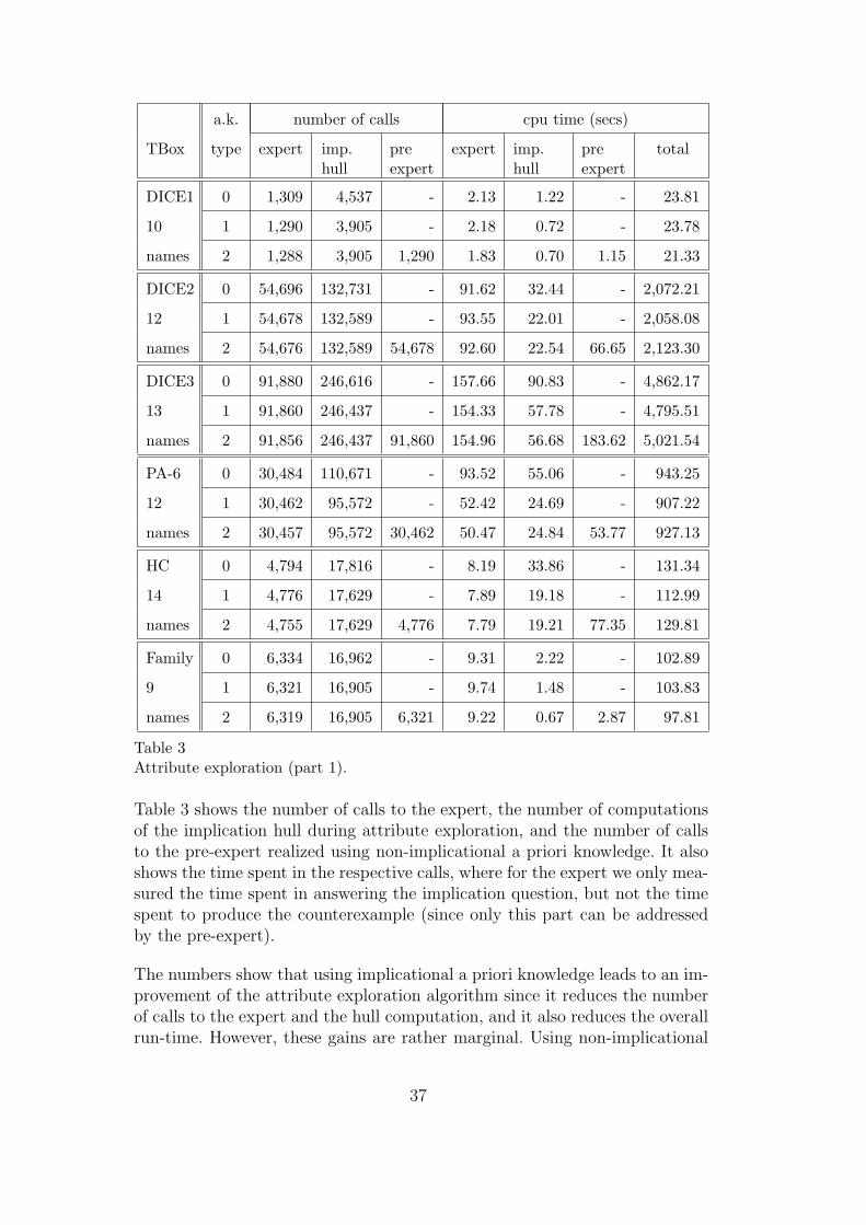
a.k. number of calls cpu time (secs)

TBox type expert imp.hull

preexpert

expert imp.hull

preexpert

total

DICE1 0 1,309 4,537 - 2.13 1.22 - 23.81

10 1 1,290 3,905 - 2.18 0.72 - 23.78

names 2 1,288 3,905 1,290 1.83 0.70 1.15 21.33

DICE2 0 54,696 132,731 - 91.62 32.44 - 2,072.21

12 1 54,678 132,589 - 93.55 22.01 - 2,058.08

names 2 54,676 132,589 54,678 92.60 22.54 66.65 2,123.30

DICE3 0 91,880 246,616 - 157.66 90.83 - 4,862.17

13 1 91,860 246,437 - 154.33 57.78 - 4,795.51

names 2 91,856 246,437 91,860 154.96 56.68 183.62 5,021.54

PA-6 0 30,484 110,671 - 93.52 55.06 - 943.25

12 1 30,462 95,572 - 52.42 24.69 - 907.22

names 2 30,457 95,572 30,462 50.47 24.84 53.77 927.13

HC 0 4,794 17,816 - 8.19 33.86 - 131.34

14 1 4,776 17,629 - 7.89 19.18 - 112.99

names 2 4,755 17,629 4,776 7.79 19.21 77.35 129.81

Family 0 6,334 16,962 - 9.31 2.22 - 102.89

9 1 6,321 16,905 - 9.74 1.48 - 103.83

names 2 6,319 16,905 6,321 9.22 0.67 2.87 97.81

Table 3Attribute exploration (part 1).

Table 3 shows the number of calls to the expert, the number of computationsof the implication hull during attribute exploration, and the number of callsto the pre-expert realized using non-implicational a priori knowledge. It alsoshows the time spent in the respective calls, where for the expert we only mea-sured the time spent in answering the implication question, but not the timespent to produce the counterexample (since only this part can be addressedby the pre-expert).

The numbers show that using implicational a priori knowledge leads to an im-provement of the attribute exploration algorithm since it reduces the numberof calls to the expert and the hull computation, and it also reduces the overallrun-time. However, these gains are rather marginal. Using non-implicational

37

a priori knowledge in the way we currently do is not advisable: there is onlya very moderate reduction of the number of calls to the expert, and the ad-ditional calls to the pre-expert often take more time than is is gained thisway. However, things may change if one uses a highly optimized propositionalreasoner to realize the pre-expert, and when calls to the expert become moreexpensive for larger background TBoxes.

What Table 3 also shows is that most of the time spent in attribute explo-ration is not spent answering implication questions or computing the implica-tion hull. The major culprit actually turns out to be the computation of theoperation Bi 7→ B′′

i . The reason is that the number of objects in the contextscomputed during attribute exploration becomes very large. For example, con-sider the DICE3 TBox. There, we have 91,880 calls to the expert, but only27 implications (see Table 4 below). This means that in all but 27 cases, theexpert produces a counterexample. Thus, the final context consists of 91,853objects. In addition to the problem caused by the large number of objectswhen computing the operation Bi 7→ B′′

i , the expert also spends quite sometime actually producing the counterexample, i.e., checking by subsumptiontests which attributes the counterexample satisfies and which it does not. Asmentioned above, this time was not measured in the column for the run-timeof the expert. The high number of calls to the expert and the long run-timesfor the TBoxes DICE-2, DICE-3, and PA-6 are due to the fact that for theseTBoxes (i) the number of concept names is relatively high, while (ii) thereare not many subsumption relationships between conjunctions of (negated)concept names. For the TBox HC, the measured values are much lower, al-though this TBox contains more concept names. As mentioned before, HCwas built to contain new subsumption relationships between conjunctions of(negated) concept names, i.e., relationships that do not directly follow from thesubsumption relationships between the names. Thus, there are less counterex-amples and more implications. This is the reason why computing the extendedsubsumption hierarchy for this TBox takes much less time compared to theTBoxes DICE-2, DICE-3, and PA-6.

Table 4 shows the sizes of the final set of implications computed by the at-tribute exploration algorithm. Since the third variant of the attribute explo-ration algorithm (type 2) only “optimizes” the expert, but does not change thethe attribute exploration process, the results for it coincide with the secondvariant (type 1). Thus, it is not explicitly included in the table. For type 1 wedistinguish between the set of all implications and the ones computed duringthe exploration process. For example, for PA-6 we had 24 implications as apriori knowledge and computed 7 additional implications.

The most interesting result that can be drawn from this table is that thenumber of implications stays rather small (in particular compared to the hugenumber of objects in the final context). Consequently, computing implication

38

a.k. size of base

TBox type computed total

DICE1 0 24 24

10 names 1 3 25

DICE2 0 21 21

12 names 1 3 22

DICE3 0 27 27

13 names 1 6 28

a.k. size of base

TBox type computed total

PA-6 0 31 31

12 names 1 7 31

HC 0 56 56

14 names 1 32 62

Family 0 16 16

9 names 1 3 16

Table 4Attribute exploration (part 2).

hulls for these sets of implications will be fast (see Subsection 6.4 below).

6.3 Computing the gcs

The first set of experiments was used to find out whether usingALE-expansionleads to a more specific common subsumer. To this purpose we ran experimentsw.r.t. all six background TBoxes, computing the gcs of randomly generatedALE(T )-concept descriptions once with ALE-expansion and once without,and comparing the computed common subsumers w.r.t. subsumption. Table 5summarizes the obtained results: the entries describe how often

• the gcs computed from the ALE-expanded concept descriptions was equiva-lent to the gcs computed from the unexpanded descriptions (ALE-expansionsame);

• the gcs computed from the ALE-expanded concept descriptions was strictlymore specific than the gcs computed from the unexpanded descriptions(ALE-expansion better);

• the gcs computed from the ALE-expanded concept descriptions was morespecific than > whereas the gcs computed from the unexpanded descriptionswas equivalent to > (ALE-expansion much better).

The results show that in the majority of the tests ALE-expansion does notyield a more specific common subsumer. Nevertheless, the fact that in 13% ofall tests ALE-expansion results in a more specific common subsumer justifiesusing it. The comparison with > was done since the common subsumer > istotally useless, and thus the last column of Table 5 shows how often ALE-expansion generated a useful result whereas the common subsumer obtainedfrom the unexpanded descriptions was useless.

39

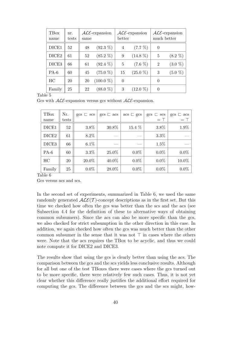
TBoxname

nr.tests

ALE-expansionsame

ALE-expansionbetter

ALE-expansionmuch better

DICE1 52 48 (92.3 %) 4 (7.7 %) 0

DICE2 61 52 (85.2 %) 9 (14.8 %) 5 (8.2 %)

DICE3 66 61 (92.4 %) 5 (7.6 %) 2 (3.0 %)

PA-6 60 45 (75.0 %) 15 (25.0 %) 3 (5.0 %)

HC 20 20 (100.0 %) 0 0

Family 25 22 (88.0 %) 3 (12.0 %) 0Table 5Gcs with ALE-expansion versus gcs without ALE-expansion.

TBoxname

Nr.tests

gcs < scs gcs < acs acs < gcs gcs < scs= >

gcs < acs= >

DICE1 52 3.8% 30.8% 15.4 % 3.8% 1.9%

DICE2 61 8.2% — — 3.3% —

DICE3 66 6.1% — — 1.5% —

PA-6 60 3.3% 25.0% 0.0% 0.0% 0.0%

HC 20 20.0% 40.0% 0.0% 0.0% 10.0%

Family 25 0.0% 28.0% 0.0% 0.0% 0.0%Table 6Gcs versus acs and scs.

In the second set of experiments, summarized in Table 6, we used the samerandomly generated ALE(T )-concept descriptions as in the first set. But thistime we checked how often the gcs was better than the scs and the acs (seeSubsection 4.4 for the definition of these to alternative ways of obtainingcommon subsumers). Since the acs can also be more specific than the gcs,we also checked for strict subsumption in the other direction in this case. Inaddition, we again checked how often the gcs was much better than the othercommon subsumer in the sense that it was not > in cases where the otherswere. Note that the acs requires the TBox to be acyclic, and thus we couldnote compute it for DICE2 and DICE3.

The results show that using the gcs is clearly better than using the acs. Thecomparison between the gcs and the scs yields less conclusive results. Althoughfor all but one of the test TBoxes there were cases where the gcs turned outto be more specific, there were relatively few such cases. Thus, it is not yetclear whether this difference really justifies the additional effort required forcomputing the gcs. The difference between the gcs and the scs might, how-

40

ever, become more important for larger knowledge bases with more complexrelationships between the concept names occurring in them. This is also sup-ported by the results for the handcrafted TBox HC, which was designed tocontain such relationships.

6.4 Computing the supremum

Table 7 shows the time spent in supremum calls that were generated duringthe computation of the gcs in the experiments described in the previous sub-section. We measured the run-time for three different methods of computingthe supremum:

Type 0: The supremum is computed by building the implication hull w.r.t.the implication base computed without using a priori knowledge duringattribute exploration.

Type 1: The supremum is computed by building the implication hull w.r.t.the implication base computed using a priori knowledge during attributeexploration.

Type 2: The supremum is computed naıvely using iterated calls of the sub-sumption algorithm, as sketched at the end of Subsection 4.2.

Since the implication base computed with a priori knowledge is usually a bitlarger than the one without, using this base takes a bit longer, but in bothcases the supremum is computed very fast. In contrast, the naıve approach istwo orders of magnitude slower. Thus, it really pays to have the implicationbase available.

7 Related and future work

In a preliminary version of this paper [50], we have considered computing thelcs in EL w.r.t. a background ALC-terminology. We have shown that the lcsw.r.t. acyclic TBoxes always exists in this setting, and that the lcs w.r.t. gen-eral TBoxes need not exist. We have also sketched a practical approach forcomputing good common subsumers similar to the one described above. SinceEL does not allow for atomic negation, we only had to consider conjunctions ofconcepts names (no negated names). The present version of the paper (whichwas first published in a shorter version as [58]) improves on this by using theconsiderably more expressive DL ALE in place of EL (which makes the proofof Theorem 12 much harder), by extending the approach for computing thesubsumption lattice of all conjunctions of concept names to conjunctions ofconcept names and negated concept names, by using attribute exploration

41

exp. cpu time (secs) base

TBox type average total size

DICE1 0 0.00015 0.01 24

67 supremum 1 0.0003 0.02 25

calls 2 0.03045 2.04 –

DICE2 0 0.00016 0.02 21

121 supremum 1 0.00016 0.02 22

calls 2 0.04330 5.24 –

DICE3 0 0.00039 0.04 27

101 supremum 1 0.00049 0.05 28

calls 2 0.0403 4.07 –

PA-6 0 0.00046 0.11 31

237 supremum 1 0.00046 0.11 31

calls 2 0.04810 11.40 –

HC 0 0.00166 0.07 56

42 supremum 1 0.00238 0.10 62

calls 2 0.06 2.52 –

Family 0 0.0001 0.01 16

98 supremum 1 0.0002 0.02 16

calls 2 0.03775 3.70 –Table 7Computing the supremum of conjunctions of (negated) concept names.

with a priori knowledge and ALE-expansion, and by providing first experi-mental results on the run-time for computing the subsumption lattice, and onthe quality of the computed gcs (compared to other approaches for computingcommon subsumers).

It should be noted that formal concept analysis and attribute exploration havealready been applied in a different context to the problem of computing theleast common subsumer. In [59], the following problem is addressed: givena finite collection C of concept descriptions, compute the subsumption hier-archy of all least common subsumers of subsets of C. Again, this extendedsubsumption hierarchy can be computed by defining a formal context whoseconcept lattice is isomorphic to the subsumption lattice we are interested in,and then applying attribute exploration (see [59] for details). In [53], it is

42

shown that this approach and the one used in the present paper can be seenas two instances of a more abstract approach.

On the theoretical side, the main topic for future research is to try to findexact algorithms for computing the least common subsumer that are betterthan the brute-force algorithm sketched in the proof of Theorem 12. On thepractical side, we will, on the one hand, try to improve the formal conceptanalysis part of our approach by (i) improving the implementation of the at-tribute exploration algorithm such that it can handle larger knowledge bases,and (ii) checking whether efficient SAT solvers (see, e.g., [60]) can be used tohandle non-implicational a priori knowledge. On the other hand, we want tointegrate the implementation of the scs computation into our non-standardinference system Sonic [61]. So far, this system offers the lcs and approxima-tion inference as a plug-in of the ontology editor OilEd. The integration ofthe scs in Sonic will enable us to see whether this fairly inexpensive way ofcomputing a common subsumer is already useful for practical applications, orwhether the more expensive gcs or lcs is needed.

References

[1] F. Baader, D. Calvanese, D. McGuinness, D. Nardi, P. F. Patel-Schneider(Eds.), The Description Logic Handbook: Theory, Implementation, andApplications, Cambridge University Press, 2003.

[2] M. R. Quillian, Word concepts: A theory and simulation of some basiccapabilities, Behavioral Science 12 (1967) 410–430, republished in [62].

[3] M. Minsky, A framework for representing knowledge, in: J. Haugeland (Ed.),Mind Design, The MIT Press, 1981, a longer version appeared in The Psychologyof Computer Vision (1975). Republished in [62].

[4] W. A. Woods, J. G. Schmolze, The KL-ONE family, in: F. W. Lehmann (Ed.),Semantic Networks in Artificial Intelligence, Pergamon Press, 1992, pp. 133–178, published as a special issue of Computers & Mathematics with Applications,Volume 23, Number 2–9.

[5] R. Moller, V. Haarslev, Description logic systems, in: [1], 2003, pp. 282–305.

[6] F. Donini, Complexity of reasoning, in: [1], 2003, pp. 96–136.

[7] I. Horrocks, Using an expressive description logic: FaCT or fiction?, in: Proc.of the 6th Int. Conf. on Principles of Knowledge Representation and Reasoning(KR’98), 1998, pp. 636–647.

[8] V. Haarslev, R. Moller, RACER system description, in: Proc. of the Int. JointConf. on Automated Reasoning (IJCAR 2001), 2001.

43

[9] I. Horrocks, Implementation and optimization techniques, in: [1], 2003, pp. 306–346.

[10] I. Horrocks, The FaCT system, in: H. de Swart (Ed.), Proc. of the 2nd Int.Conf. on Analytic Tableaux and Related Methods (TABLEAUX’98), Vol. 1397of Lecture Notes in Artificial Intelligence, Springer-Verlag, 1998, pp. 307–312.

[11] V. Haarslev, R. Moller, High performance reasoning with very large knowledgebases: A practical case study, in: Proc. of the 17th Int. Joint Conf. on ArtificialIntelligence (IJCAI 2001), 2001.

[12] F. Baader, I. Horrocks, U. Sattler, Description logics for the semantic web, KI– Kunstliche Intelligenz 2002 (4).

[13] F. Baader, I. Horrocks, U. Sattler, Description logics, in: S. Staab, R. Studer(Eds.), Handbook on Ontologies, International Handbooks in InformationSystems, Springer–Verlag, Berlin, Germany, 2003, pp. 3–28.

[14] T. Berners-Lee, J. Hendler, O. Lassila, The semantic Web, Scientific American284 (5) (2001) 34–43.

[15] I. Horrocks, P. F. Patel-Schneider, F. van Harmelen, From SHIQ and RDF toOWL: The making of a web ontology language, Journal of Web Semantics 1 (1)(2003) 7–26.

[16] I. Horrocks, U. Sattler, S. Tobies, Practical reasoning for very expressivedescription logics, J. of the Interest Group in Pure and Applied Logic 8 (3)(2000) 239–264.

[17] I. Horrocks, U. Sattler, Ontology reasoning in the SHOQ(D) description logic,in: Proc. of the 17th Int. Joint Conf. on Artificial Intelligence (IJCAI 2001),Morgan Kaufmann, Los Altos, 2001.

[18] S. Bechhofer, I. Horrocks, C. Goble, R. Stevens, OilEd: A reason-able ontologyeditor for the semantic web, in: F. Baader, G. Brewka, T. Eiter (Eds.), KI-2001: Advances in Artificial Intelligence, Vol. 2174 of Lecture Notes in ArtificialIntelligence, Springer-Verlag, 2001, pp. 396–408.

[19] H. Knublauch, R. W. Fergerson, N. F. Noy, M. A. Musen, The Protege OWLplugin: An open development environment for semantic web applications, in:Proceedings of the Third International Semantic Web Conference, Hiroshima,Japan, 2004.

[20] R. Kusters, Non-standard Inferences in Description Logics, Vol. 2100 of LectureNotes in Artificial Intelligence, Springer-Verlag, 2001.

[21] F. Baader, R. Kusters, Computing the least common subsumer and the mostspecific concept in the presence of cyclic ALN -concept descriptions, in: Proc.of the 22nd German Annual Conf. on Artificial Intelligence (KI’98), Vol. 1504of Lecture Notes in Computer Science, Springer-Verlag, 1998, pp. 129–140.

[22] F. Baader, R. Kusters, R. Molitor, Computing least common subsumers indescription logics with existential restrictions, in: Proc. of the 16th Int. JointConf. on Artificial Intelligence (IJCAI’99), 1999, pp. 96–101.

44

[23] W. W. Cohen, H. Hirsh, Learning the CLASSIC description logics: Theoreticaland experimental results, in: J. Doyle, E. Sandewall, P. Torasso (Eds.), Proc. ofthe 4th Int. Conf. on the Principles of Knowledge Representation and Reasoning(KR’94), 1994, pp. 121–133.

[24] M. Frazier, L. Pitt, CLASSIC learning, Machine Learning 25 (1996) 151–193.

[25] R. Kusters, R. Molitor, Computing least common subsumers in ALEN , in:Proc. of the 17th Int. Joint Conf. on Artificial Intelligence (IJCAI 2001), 2001,pp. 219–224.

[26] R. Kusters, R. Molitor, Approximating most specific concepts in descriptionlogics with existential restrictions, in: F. Baader, G. Brewka, T. Eiter (Eds.),Proceedings of the Joint German/Austrian Conference on Artificial Intelligence(KI 2001), Vol. 2174 of Lecture Notes in Artificial Intelligence, Springer-Verlag,Vienna, Austria, 2001, pp. 33–47.

[27] R. Kusters, A. Borgida, What’s in an attribute? Consequences for the leastcommon subsumer, J. of Artificial Intelligence Research 14 (2001) 167–203.

[28] F. Baader, Least common subsumers and most specific concepts in a descriptionlogic with existential restrictions and terminological cycles, in: G. Gottlob,T. Walsh (Eds.), Proceedings of the 18th International Joint Conference onArtificial Intelligence, Morgan Kaufmann, 2003, pp. 319–324.

[29] S. Brandt, A.-Y. Turhan, R. Kusters, Extensions of non-standard inferencesfor description logics with transitive roles, in: M. Vardi, A. Voronkov (Eds.),Proceedings of the 10th International Conference on Logic for Programmingand Automated Reasoning (LPAR’03), Vol. 2850 of Lecture Notes in ArtificialIntelligence, Springer-Verlag, 2003, pp. 122–136.

[30] A. Rector, I. Horrocks, Experience building a large, re-usable medicalontology using a description logic with transitivity and concept inclusions,in: Proceedings of the Workshop on Ontological Engineering, AAAI SpringSymposium (AAAI’97), AAAI Press, Stanford, CA, 1997.

[31] S. Schultz, U. Hahn, Knowledge engineering by large-scale knowledge reuse—experience from the medical domain, in: A. G. Cohn, F. Giunchiglia, B. Selman(Eds.), Proc. of the 7th Int. Conf. on Principles of Knowledge Representationand Reasoning (KR’2000), Morgan Kaufmann, 2000, pp. 601–610.

[32] B. Ganter, Finding all closed sets: A general approach, Order 8 (1991) 283–290.

[33] B. Ganter, Attribute exploration with background knowledge, TheoreticalComputer Science 217 (2) (1999) 215–233.

[34] B. Ganter, R. Krauße, Pseudo models and propositional Horn inference, Tech.Rep. MATH-AL-15-1999, Institut fur Algebra, Technische Universitat Dresden,Dresden, Germany (1999).

[35] B. Ganter, R. Wille, Formal Concept Analysis: Mathematical Foundations,Springer-Verlag, Berlin, 1999.

45

[36] F. M. Donini, B. Hollunder, M. Lenzerini, A. M. Spaccamela, D. Nardi, W. Nutt,The complexity of existential quantification in concept languages, ArtificialIntelligence 2–3 (1992) 309–327.

[37] M. Schmidt-Schauß, G. Smolka, Attributive concept descriptions withcomplements, Artificial Intelligence 48 (1) (1991) 1–26.

[38] F. Baader, Terminological cycles in a description logic with existentialrestrictions, in: G. Gottlob, T. Walsh (Eds.), Proceedings of the 18thInternational Joint Conference on Artificial Intelligence, Morgan Kaufmann,2003, pp. 325–330.

[39] S. Brandt, Polynomial time reasoning in a description logic with existentialrestrictions, GCI axioms, and—what else?, in: R. L. de Mantaras, L. Saitta(Eds.), Proc. of the 16th Eur. Conf. on Artificial Intelligence (ECAI 2004),2004, pp. 298–302.

[40] C. Lutz, Complexity of terminological reasoning revisited, in: Proc. of the 6thInt. Conf. on Logic for Programming and Automated Reasoning (LPAR’99),Vol. 1705 of Lecture Notes in Artificial Intelligence, Springer-Verlag, 1999, pp.181–200.

[41] K. Schild, A correspondence theory for terminological logics: Preliminaryreport, in: Proc. of the 12th Int. Joint Conf. on Artificial Intelligence (IJCAI’91),1991, pp. 466–471.

[42] F. Baader, S. Brandt, C. Lutz, Pushing the EL envelope, in: Proceedings of theNineteenth International Joint Conference on Artificial Intelligence IJCAI-05,Morgan-Kaufmann Publishers, Edinburgh, UK, 2005.

[43] B. Nebel, Terminological reasoning is inherently intractable, ArtificialIntelligence 43 (1990) 235–249.

[44] S. Brandt, R. Kusters, A.-Y. Turhan, Approximation and difference indescription logics, in: D. Fensel, F. Giunchiglia, D. McGuiness, M.-A. Williams(Eds.), Proceedings of the Eighth International Conference on Principles ofKnowledge Representation and Reasoning (KR2002), Morgan Kaufman, SanFrancisco, CA, 2002, pp. 203–214.

[45] F. Baader, R. Kusters, R. Molitor, Rewriting concepts using terminologies, in:Proc. of the 7th Int. Conf. on Principles of Knowledge Representation andReasoning (KR’2000), 2000, pp. 297–308.

[46] G. Stumme, R. Wille, Begriffliche Wissensverarbeitung – Methoden undAnwendungen, Springer-Verlag, 2000.

[47] W. F. Dowling, J. H. Gallier, Linear-time algorithms for testing the satisfiabilityof propositional horn formulae, Journal of Logic Programming 1 (3) (1984) 267–284.

[48] D. Maier, The Theory of Relational Databases, Computer Science Press,Potomac, Maryland, 1983.

46

[49] V. Duquenne, Contextual implications between attributes and somerepresentational properties for finite lattices, in: B. Ganter, R. Wille, K. E.Wolf (Eds.), Beitrage zur Begriffsanalyse, B.I. Wissenschaftsverlag, Mannheim,1987, pp. 213–239.

[50] F. Baader, B. Sertkaya, A.-Y. Turhan, Computing the least common subsumerw.r.t. a background terminology, in: Proceedings of the 2004 InternationalWorkshop on Description Logics (DL2004), 2004.

[51] F. Baader, Computing a minimal representation of the subsumption lattice of allconjunctions of concepts defined in a terminology, in: G. Ellis, R. A. Levinson,A. Fall, V. Dahl (Eds.), Knowledge Retrieval, Use and Storage for Efficiency:Proc. of the 1st Int. KRUSE Symposium, 1995, pp. 168–178.

[52] F. Baader, U. Sattler, An overview of tableau algorithms for description logics,Studia Logica 69 (2001) 5–40.

[53] F. Baader, B. Sertkaya, Applying formal concept analysis to description logics,in: P. Eklund (Ed.), Proceedings of the 2nd International Conference on FormalConcept Analysis (ICFCA 2004), Vol. 2961 of Lecture Notes in ComputerScience, Springer-Verlag, Sydney, Australia, 2004, pp. 261–286.

[54] G. Stumme, Attribute exploration with background implications andexceptions, in: H.-H. Bock, W. Polasek (Eds.), Data Analysis and InformationSystems: Statistical and Conceptual Approaches (GfKl’95), Vol. 7 of Studies inClassification, Data Analysis, and Knowledge Organization, 1996, pp. 457–469.

[55] R. Cornet, A. Abu-Hanna, Using description logics for managing medicalterminologies, in: M. Dojat, E. Keravnou, P. Barahona (Eds.), 9th Conferenceon Artificial Intelligence in Medicine in Europe (AIME 2003), Lecture Notes inComputer Science, Springer-Verlag, 2003, pp. 61–70.

[56] B. Hollunder, F. Baader, Qualifying number restrictions in concept languages,Tech. Rep. RR-91-03, Deutsches Forschungszentrum fur Kunstliche Intelligenz(DFKI), Kaiserslautern (Germany), an abridged version appeared in Proc.of the 2nd Int. Conf. on the Principles of Knowledge Representation andReasoning (KR’91)(1991).

[57] G. Schopfer, A. Yang, L. von Wedel, W. Marquardt, CHEOPS: Atool-integration platform for chemical process modelling and simulation,International Journal on Software Tools for Technology Transfer 6 (3) (2004)186–202.

[58] F. Baader, B. Sertkaya, A.-Y. Turhan, Computing the least common subsumerw.r.t. a background terminology, in: J. J. Alferes, J. A. Leite (Eds.), Proceedingsof the 9th European Conference on Logics in Artificial Intelligence (JELIA2004), Vol. 3229 of Lecture Notes in Computer Science, Springer-Verlag, Lisbon,Portugal, 2004, pp. 400–412.

[59] F. Baader, R. Molitor, Building and structuring description logic knowledgebases using least common subsumers and concept analysis,

47

in: B. Ganter, G. Mineau (Eds.), Conceptual Structures: Logical, Linguistic,and Computational Issues – Proceedings of the 8th International Conferenceon Conceptual Structures (ICCS2000), Vol. 1867 of Lecture Notes in ArtificialIntelligence, Springer-Verlag, 2000, pp. 290–303.

[60] L. Zhang, S. Malik, The quest for efficient Boolean satisfiability solvers, in:A. Voronkov (Ed.), 18th International Conference on Automated Deduction(CADE-18), Vol. 2392 of Lecture Notes in Computer Science, Springer-Verlag,Copenhagen, Denmark, 2002, pp. 295–313.

[61] A.-Y. Turhan, C. Kissig, Sonic — Non-standard inferences go OilEd, in:D. Basin, M. Rusinowitch (Eds.), Proc. of the Int. Joint Conf. on AutomatedReasoning (IJCAR 2004), Vol. 3097 of Lecture Notes in Computer Science,Springer-Verlag, 2004, pp. 321–325.

[62] R. J. Brachman, H. J. Levesque (Eds.), Readings in Knowledge Representation,Morgan Kaufmann, Los Altos, 1985.

48