See other formats

Full text of "Wind tunnels and their instrumentation"

NASA

TT

F‐3U6

c.l

S.M.Gorlin and I.I.SIezinger

WIND TUNNELS

ANDTHEIR

INSTRUMENTATION

LOAN COPY: RETURN ^

AFVVL (WUL‐21 —

KIRTLAND AFBr N Mtg^ £

g 30

 

tr II >

Oa 3

03 . "*

•n

TRANSLATED FROM RUSSIAN

\ ‐ ■ I

Published for the National Aeronautics and Space Administration, U.S.A.

and the National Science Foundation, Washington, D.C.

by the Israel Program for Scientific Translations

TECH LIBRARY KAFB, NM

D0t>QQ51

S. M, GORLIN and 1. 1. SLEZINGER

 

WIND TUNNELS

AND

THEIR INSTRUMENTATION

(Aeromekhanicheskie izmerenia. Metody i pribory)

Izdatel'stvo "Nauka"

Moskva 1964

Translated from Russian

Israel Program for Scientific Translations

Jerusalem 1966

NASA TTP‐346

TT 66‐51026

Published Pursuant to an Agreement with

THE U.S. NATIONAL AERONAUTICS AND SPACE ADMINISTRATION

and

THE NATIONAL SCIENCE FOUNDATION, WASHINGTON, D. C.

 

Copyright © 1966

Israel Program for Scientific Translations Ltd.

IPST Cat. No. 1680

Translated by P. Boltiansky, E.E.

Edited by IPST Staff

Printed in Jerusalem by S.Monson

Binding: Wiener Bindery Ltd.. Jerusalem

Price: $ 9. 00

Available from the

U.S. DEPARTMENT OF COMMERCE

Clearinghouse for Federal Scientific and Technical Information

Springfield, Va. 22151

Xn/13/4.5

TABLE OF CONTENTS

FOREWORD V

 

INTRODUCTION 1

Chapter I. THE DESIGN OF MODELS FOR AERODYNAMIC EXPERIMENTS , . 3

§ 1, Criteria of similarity 3

§ 2. Coordinate axes. Aerodynamic coefficients 8

Chapter n. WIND TUNNELS AND INSTALLATIONS 13

§ 3. Operating principles of wind tunnels 13

§ 4. Subsonic wind tunnels. Open‐circuit tunnels 24

§ 5. Transonic tunnels 48

§ 6. Supersonic wind tunnels 63

§ 7. Hypersonic wind tunnels 86

§ 8. Wind tunnels for testing aircraft engines 115

Chapter III. WIND TUNNEL DESIGN CALCULATIONS 122

§ 9. Design of subsonic tunnels 122

§10. Gas dynamics of supersonic tunnels 142

Chapter IV. MEASUREMENT OF FLOW PARAMETERS IN WIND TUNNELS . ‐ 156

§11. Pressure measurement 160

§12. The measurement of the Mach number and flow velocity . . 173

 

§13. The measurement of flow direction 195

§14. Measurement of temperature in flow 207

§15. Measurement of density: humidity corrections 219

§16. Boundary ‐layer measurements 223

§n. Instruments for mapping distributions 232

§18. Visual and optical methods of flow distributions .... 239

Chapter V. INSTRUMENTS AND APPARATUS FOR PRESSURE MEASUREMENT . 255

§19. Liquid‐column manometers 257

§20. Mechanical manometers 270

§21. Electrical pressure transducers and micromanometers . . . 281

§22. Equipment for measuring presaute distribution. Multiple

manometers 294

§23. Transmission lag in manometric systems 310

§24. Manometric instruments for determining dimensionless

characteristics 314

Chapter VI. WIND‐TUNNEL BALANCES

§25. Wind‐tunnel balances located outside the model

 

§26. Design examples of wind‐tunnel balances •

§27. Balance elements of wind‐tunnel balances .

§28. Wind‐tunnel balances located inside the model

§29. The errors of wind‐tunnel balances. Calibration

Chapter VII. TECHNIQUES AND METHODS OF AERODYNAMIC

MEASUREMENTS

§30.

§31.

§32.

§33.

§34.

§35.

§36.

§37.

§38.

§39.

326

328

357

362

379

425

438

Adjustment of wind tunnels 438

 

Techniques and methods of balance measurements . . . 445

Determination of pressure and velocity distributions . . . 451

The testing of propellers 458

Testing of blade cascades 476

Testing of fans 490

Experimental determination of local resistances .... 496

Testing of wind turbines 503

Testing of ejectors 508

Determining rotational derivatives 510

Chapter VIII. PROCESSING THE RESULTS OF WIND‐TUNNEL TESTS ... 527

§40. Interference between tunnel and model 527

§41. Interference between model and supports 547

§42. Accuracy and reproducibility of tests 555

Chapter IX. AUTOMATIC DATA RECORDING AND PROCESSING OF

WIND‐TUNNEL MEASUREMENTS 564

§43. Methods of automatically processing measured data . . . 564

§44. Digital conversion of measured values. Digital

 

conversion of angles 569

§45. Processing the measured data on computers 586

IV

FOREWORD

Aerodynamic measuring techniques and theoretical aerohydrodynamics

have developed together. The connection is seen vividly in the works of

N.E. Joukowski and S. A. Chaplygin, who established the basis of modern

aerodynamic theory, and founded the aerodynamics laboratories of the

Soviet Union.

Although the relationship between theory and experinaent has changed as

aerodynamics developed, there has always been a paucity of experimental

data from which to develop the theory.

Some of the measuring techniques and instruments described in this

book are mentioned in the well‐known books of A. K. Martinov,

"Eksperinaental'naya aerodinamika" (Experimental Aerodynamics) (1950),

S.G.Popov, "Nekotorye zadachi eksperimental'noi aeromekhaniki" (Some

Problems in Experimental Aeromechanics) (1952), and N. A.Zaks,

"Osnovy eksperimental'noi aerodinamiki" (The Basis of Experimental

Aerodynamics) (1957). In these textbooks for advanced students measuring

techniques and instruments are necessarily described only briefly and in

passing. R. C. Pankhurst and D. W. Holder discuss a wide range of

experimental problems in their textbook "Wind ‐Tunnel Technique" (1952),

but the treatment is general and sometimes superficial. Since the

 

publication of these works the technology of aerodynamics has advanced

greatly.

We try in this book to treat systematically certain modern techniques of

aerodynamic measurement, formerly described only in periodicals. We

have made wide use of experience in the USSR and abroad, selecting

material to enable readers with a knowledge of theoretical aerodynamics

to become familiar with experimental practice and with the instruments

and apparatus used in practice.

The book is intended mainly for experimental ‐research workers in

aerodynamics and for those using their results and also for students of

fluid dynamics. We think that engineers and technicians designing and

constructing aerodynamic installations, and developing measuring equipment,

will also find the book useful.

Chapters I, II, III, VII, and VIII were written by S, M. Gorlin and

Chapters IV, V, VI, IX and Sections 7 and 34 by I. I. Slezinger.

S.M.G.

I.I.S.

INTRODUCTION

The development of fluid mechanics involves observation and study of

the physical phenomena which form the basis of the theory. Experimental

aerodynamics serve to check the existing theory, and also its extension.

On the other hand, theoretical developments strongly influence experimental

techniques, installations and measuring equipnaent.

 

Since aircraft first appeared aerodynanmics have been directed toward the

study of increasingly large flight speeds. There has been a corresponding

development of equipment and techniques for experimental research and for

measurement. The type of installation and the techniques currently used

depend on the flight speed in the five ranges:

1. Low subsonic speeds [Incompressible flow].

2. High subsonic speeds [Subsonic compressible flow].

3. Transonic speeds.

4. Supersonic speeds.

5. Hypersonic speeds.

Experimental aerodynamics are at low speeds are based on the

fundamental work of N. E. Joukowski, L, Prandtl, and other leading

scientists. This speed range is still important for research in industrial

aerodynamics, surface vehicles, and the take‐off and landing

characteristics of aircraft. There are low‐speed wind tunnels, of

comparatively low power, in almost every university and institute of

advanced learning. For simulating natural conditions in the testing of

aircraft, large aerodynamics laboratories of scientific research institutes

possess low‐speed wind tunnels whose powers extend to tens and even

hundreds of megawatts. The techniques for measuring forces, pressures,

and speeds, and for visual observation of the flow around bodies at low

speeds, are widely used in research at higher speeds, and have merited

extensive treatment in this book.

The study of flight at high subsonic speeds, which first became important

about 1930, demands considerably more power and complicated equipment,

because as speed increases, the compressibility of the air becomes as

important as its viscosity. Variable ‐density wind tunnels are therefore

 

used which must have automatic instrumentation and control and permit

measurements of a wide range of parameters. The optical techniques

developed for this speed range are even more important at still higher

speeds.

We have paid special attention to transonic techniques because of the

acoustic effects of aircraft flying at speeds near the velocity of sound.

Important techniques are described for measuring parameters and

calculating effects which cannot be neglected in experiments in this speed

range. We also describe the design of instrumentation for transonic

installations.

■■niiiiiii IN

Even more involved are supersonic wind tunnels, where the power may

reach tens, and even hundreds, of megawatts. Measuring techniques,

developed for use at lower speeds, can still, with care, be used, but

optical techniques become more important, and supplementary techniques

must be introduced. The installations are far more expensive; a

considerable part of the book is devoted to the use of automatic measuring

and data ‐processing techniques which thus become economical.

Hypersonic speeds, only lately being studied, involve high temperatures

and physicochemical processes in gases. They demand a new approach

to wind‐tunnel design; techniques and instrumentation are being evolved

rapidly, and their full description would justify a separate volume. Here

we have merely reviewed this aspect of the subject in order to acquaint

readers with the trends.

Within each of the five speed ranges it is impossible to separate sharply

 

measuring techniques and use of equipment from installation design. We

have therefore alloted individual chapters to the description of aerodynamic

research installations, to the measurement of the various flow parameters,

to wind‐tunnel balances, etc. We hope that this method of presentation will

permit the reader to study each problem in detail, while avoiding the

repetition which would inevitably follow from a division of the material by

speed range. An exception has been made in the chapter on hypersonic

speeds, which combines a brief description of experimental installations anc

common measuring techniques.

Chapter I

THE DESIGN OF MODELS FOR AERODYNAMIC

EXPERIMENTS

§ 1 . CRITERIA OF SIMILARITY

It is very difficult to reproduce flight conditions exactly in aerodynamic

experiments, whether the body is moving through a stationary gas or the

gas past a stationary body. Models are therefore commonly used in wind

tunnels of limited dimensions, to predict the behavior of prototypes in

flight.

The accuracy of predictions from tests on models depends on the

fidelity with which flow around the model or in a channel of limited size

reproduces the flow around the full‐scale body or in the full‐scale channel,

i. e., it depends on the fulfilment of "criteria of similarity. "

As L.I. Sedov III has pointed out, scaling‐down will be sucessful if we

are able to substitute for the phenomena which interest us, closely analogous

phenomena on another scale. Scale‐naodel testing is thus based on studying

physically similar phenomena. Geometric similarity* is fundamental to

 

aerodynamic experimentation. The coefficient of geometric similarity, i.e.,

the geometric scale factor of the model, is the ratio of the dimensions of

the model to the dimensions of the (geometrically similar) natural object.

Mechanical or physical similarity implies that we should be able to calculate

physical effects from observations on a different scale. However, certain

conditions must be fulfilled if this similarity is to be achieved.

We define two systems as being similar to each other if all the physical

characteristics at corresponding points** in the two systems have the same

relationship. The relationship between masses, velocities, viscosities,

and other parameters in two such systems can be derived by considering

the conditions and relationships within each system at any instant.

For the flow of viscous, incompressible fluids such considerations /2/

show that at corresponding points within the systems mechanical

similarity demands that

^» __ •»! . Pt __ Pi

Two bodies are "geometrically similar" if the ratio of all corresponding linear dimensions is uniform.

By corresponding points of similar systems we understand points which are similarly placed geometrically

in relation to geometrically similar bodies within the two systems.

Here / is a representative time, I a representative length, p the density,

V the coefficient of kinematic viscosity, Z the body force [gravity,

centrifugal force, etc.; Z has the dimensions of acceleration], V is the

velocity, p the pressure; the subscripts 1 and 2 refer to the first and

second system, respectively.

The first of these relationships is the condition for kinematic similarity.

 

The other esqaressions define the conditions of dynamical similarity, i, e.,

the similarity of forces arising during motion.

To ensure similarity when studying rotational m.otion of liquids or

bodies (the flow of liquid around a rotating propellor, or the velocity

fluctuations in a wake) the [dimensionless] coefficient J~ must be the

sam^e for both model and prototype! In practice, for cyclic phenom.ena,

we use Strouhal's criterion that

4=Sh,

be constant, n being the frequency and V the free ‐stream velocity of the

flow. For example, when comparing performance and efficiencies of

propellers we maintain constancy of the advance ratio

Here ric is the nunaber of revolutions of the screw; the advance ratio,

relating the flight speed to the circumferential velocity of the blade tips,

is a form of the Strouhal number, which ensures similarity of the systems.

For steady flow of viscous, incompressible liquids two conditions of

similarity apply. Both the Froude number

and the Reynolds number

gi, gt, ^'^'

 

must be the same for the two systems.

Thus, in aviscous, connpressibleliquidunder the action of the force of

gravity only, two systems which have the same Reynolds and Froude numbers

are similar. Whenever we mention "similarity" phenomena, we consider

geometrically similar bodies, similarly oriented with respect to the flow.

When there are no body forces the criteria of simiilarity are greatly

simplified; two flows will then be sim.ilar if the Reynolds numbers are the

same. The aerodynamic forces on a body depend in this case only on the

Reynolds number and the orientation of the body to the flow.

When allowance is made for inertia, viscosity, compressibility, and

thermal conductivity*, the conditions for the mechanical similarity of

motion in fluids, of geometrically similar, similarly placed solid bodies,

are more complicated. It is then necessary to maintain equality of the

• Neglecting buoyancy and radiant heat transfer.

following dimensionless parameters in the two systems:

Re = ‐. M = y==. Pr‐— .

« = — 1 ‐yr‐ and 'y •

Here M is the Mach number, which relates flight speed to the velocity

of sound a = V^xgRT",. Pr is the Prandtl nunaber; C is Sutherland's constant

(which has the dimensions of tem.perature, and for air is about 113°C)**;

 

X is the coefficient of thermal conductivity; n is the ratio of the specific

heat Cp at constant pressure to the specific heat c« at constant volume; T\, is

the absolute temperature at the surface of the body; and T is the absolute

temperature of the gas.

In som.e cases T\m T , and the parameter Ti/T may be ignored. It is

often permissible to ignore C/T , which expresses the influence of the

temperature on the viscosity and thermal conductivity^. Thus, in

studying motion through gases of equal compressibility and atomicity,

and for which the values of‐j^‐and Pr are therefore the same, similarity will be

ensured if the Reynolds and Mach numbers are the same in both gases.

These two magnitudes are the most important similarity criteria in

aerodynamics .

For an ideal, incompressible fluid, the criterion of similarity for the

pressures at corresponding points is expressed by

Pt _ Pi

PjV? P.V1 "

It thus follows that the ratio of the reactions Ri and /?j of the fluid on

geometrically similar (and similarly oriented) bodies is

^2 f2'ih

where Nw is Newton's [dimensionless] nunaber.

Newton's number defines the similarity in this case.

Thus in an ideal, incompressible fluid, the hydrodynamic forces on a

body are proportional to the square of the relative velocity (Square Law).

 

• The criterion C/T is important when the gases have different nutt^bers of atoms per molecule. For

gases of the same atomicities the values of « and Pr will be the same.

•• Sutherland's Criterion can be written

1 , C

I _>!_ "'" 273.1 ^ / T

^~ ‐ ,,C V 273.1 '

" n_

where Xo and |io correspond to T = 273.1°.

t This may be done by using the criterion

k

1 + ‐

which does not contain the dimensional constant C.

 

This law is exact only when the fluid displays ideal behavior during the

experiment.

For viscous flow of a fluid at sufficiently high Reynolds number this

law is a good approximation. At very low velocities, corresponding to

small values of Re, the influence of the viscous forces increases. When

inertia forces become negligible in comparison with the viscous drag, the

force on a body is proportional to the velocity, to the linear dixnensions of

the body, and to the coefficient of viscosity (Stokes Law). At very high

Reynolds numbers viscosity effects decrease while compressibility effects

increase. As the flow velocity increases, the forces due to the elasticity

of the gas, which depend on its pressure, become comparable with the

forces of friction, inertia etc. This causes not only a quantitative change in

the aerodynamic characteristics of the body (e.g., drag), but also in the

nature of the flow around the body. In particular, as M approaches unity,

the flow becomes locally supersonic in several regions around the body;

this causes shock waves and dissipation of energy. The pressure distribution

over the body and the moments due to the applied forces will change, and the

drag will increase sharply. It may, therefore, be best to accept variations

of the Reynolds number in experiments, to avoid changes in the Mach number

Attainment of full similarity i.e., similarity of all parameters, may

in practice be impossible. If we choose the same medium for the two

systems (e.g., water or air) at the same temperature and pressure, then

for equality of Fr, Re, and M we must have pi = p2, v, = vj, , and ^i = ^2; so

that V, = V, and /, = 4, i. e., it is impossible to obtain similar motions in the

same medium for two bodies of different sizes. Although in principle it is

possible to achieve similarity using two different liquids, it is in practice

difficult to select satisfactory values of v and a .

For these reasons it is possible to obtain only partial similarity in most

aerodynamic experiments, and we must select those criteria on which the

phenomena of interest most strongly depend.

 

In practice, geometric similarity is fully maintained only when testing

full‐scale prototypes under field conditions, or when a full‐scale model is

much smaller than the test section of the wind tunnel. In most cases the

full‐scale prototype is much larger than the tunnel, and tests must be

made on a reduced scale, at which it is difficult to reproduce faithfully the

shape of small projections and the surface finish of the prototype. This

unavoidably introduces inaccuracy, especially at high test velocities.

Dimensional tolerances in scale‐model production are therefore sometimes

tenths or hundredths of millimeters. Often, we model only the main

elements of a prototype: during comparative wing tests the ailerons and

flaps are not modelled.

In current practice the orientation of bodies in space can be reproduced

with sufficiently high accuracy (0.1 to 0.2°). The Reynolds number is an

adequate criterion of similarity at low velocities. At Mach numbers above

0.3 or 0.4 (depending on the shape of the body and its orientation in the fluid)

compressibility becomes increasingly important, and the Mach number must

be reproduced in the model test. Aerodynamic characteristics will still,

however, be considerably influenced by viscosity, and for accuracy in such

tests it is necessary to reproduce both Reynolds and Mach numbers.

When compressibility effects predominate (e. g., in a jet airplane or

rocket) it is sufficient to consider only the Mach number. In the same

medium at equal temperatures, similarity then requires only that

V, = K, .

The Reynolds number can be reproduced in a small‐scale model by

increasing the velocity in inverse proportion to the geometric scale factor,

or by increasing the density of the test medium in inverse proportion to the

product VI *. It is technically difficult to increase the velocity, since the

power required is proportional to l^^. Even when adequate power is

 

available, it must be remembered that as the velocity increases,

compressibility effects become increasingly important, so that by

maintaining the Reynolds number constant we may cause changes in the Mach

number. It is therefore common practice to reproduce the Reynolds number

by increasing the density, using variable ‐density wind tunnels, the flow

velocity being sufficient to permit simultaneous reproduction of the Mach

number.

Reproduction of the Mach number requires reproduction of the ratio of the

flow velocity to the velocity of sound. Since the velocity of sound is

a = Y*gRT it can be altered by varying either T or the product kR .

The use of other gases instead of air /3/ (e. g., Freon, which has a lower

value of kR , and requires much less power for a given M) is technically

difficult.

In this discussion of similarity criteria we have assumed that other things

being equal the same velocities in ihe two systems corresponded to equal

forces. However, there are usually velocity fluctuations superimposed on the

mean velocities in a wind tunnel. The effect of these fluctuations on the flow

and on the forces acting on the model, is in many ways analogous to the

effect of increasing the Reynolds number. The ratio of the r. m. s.

fluctuating velocity to the mean velocity of the undisturbed flow is the

turbulence level e of the undisturbed flow. It is necessary to reproduce the

value of E as closely as possible in the model, since there is no practical

way of calculating its effect on the aerodynamic characteristics. In few

wind tunnels are the values of e as low as in nature. Wind tunnels in which

e exceeds 0.5 to 1% are unsuitable for physical aerodynamic research** and

for these purposes it is usual to build special low‐turbulence tunnels.

When studying the flow of rarified gases, an important criterion of

similarity is the Knudsen number J , which is the ratio of the molecular

mean free path Z, to a representative length of the body or the thickness of

the boundary layer. Molecular motion is important to a decreasing extent

 

/4/ in free molecule flow and slip flow, and can be ignored generally in

gas dynamics (Figure 1.1).

Other characteristics of the gas or body, which may play an important

part in the motion, will each involve new criteria and similarity conditions.

For instance, in the study of a vibrating wing in a gas stream, dynamic

similarity depends on the dimensionless parameters fV^IE; G/E and wi/pP

where E is Young's modulus, G the shear modulus, and m, the mass of the

wing.

In experimental work our problem is to select those similarity criteria

which most 'influence the test results. Imperfect similarity will lead tO'

* It sliould be remembered thar the coefficient of dynamic viscosity (i is mdependent of density, and there‐

fore of pressure. The coefficient of kinematic viscosity v = |t/p depends on density, and thus on pressure.

** Investigations of the structure of the boundary layer, the position of the transition point from laminar to

turbulant flow, etc.

errors which must be evaluated when making predictions of prototype

behavior from results of tests on models. This is a particular case of the

basic problem of aerodynamics, i. e., to determine the criteria and

similarity conditions relevant to particular aerodynamic characteristics;

methods, instruments, and technology of all aeromechanical measurements

depend on the solution of this problem.

FIGURE 1.1, Flow regimes in fluids.

 

§ 2. COORDINATK AXKS. AERODYNAMIC COEFFICIENTS

In experimental aerodynanaics and aircraft design we use (as specified

in COST 1075‐41) one of the following coordinate systems: velocity, fixed, or

semifixed. All these are right‐hand systems, in which positive rotation

about any axis appears clockwise to an observer placed at the origin.

All these systems of coordinates have a common origin at the center

of gravity of the aircraft. In the velocity system of coordinates

Oxyz (Figure 1. 2) the .«: ‐axis is positive in the direction of flight. The

y ‐axis lies in the plane of symm.etry of the body; its direction is parallel

to the lift on the aircraft, being positive upwards. The z‐axis is normal to

the Oxy plane, and is positive to starboard (toward the right when looking

forward).

The fixed system of coordinates Ox\yxZ\ corresponds to the geometric axes

of the aircraft; the x, ‐axis is directed forward parallel to the horizontal

center line or the wing chord which determines the angle of attack. The

semifixed system of coordinates coincides with the velocity system when

there is no sideslip or drift (p = 0).

When the angle of sideslip changes, the semifixed system rotates with the

body around the v "axis. The velocity system of coordinates differs from the

the semifixed system by the angle of attack. The angle of attack

thus defines the orientation of i'.ie body with respect to the semifixed axes.

■ laiif III

In wind ‐tunnel tests of fixed models, the free ‐stream velocity is

opposed to the velocity of free flight; to avoid having negative drag forces

 

we sometimes use a flow coordinate system in which we replace the'x ‐axis

of the velocity system by an axis OQ in the opposite direction. The

directions of positive rotations in the flow system of coordinates are the

same as in the velocity system. In the literature the OQ axis is often

denoted by Ox for simplicity; the reader should be aware of this.

X

FIGURE 1.2. Velocity and fixed systems of coordinates

In wind‐tunnel tests in which the angles of attack and sideslip both

vary it is usual to apply not the flow system of coordinates but a modified

semifixed system in which the positive direction of the x ‐axis is reversed.

When there is no sideslip (p = 0) this semifixed "tunnel" system coincides

with the flow system, but when the sideslip angle changes the semifixed

system follows the model, rotating about Oy by the angle p . In wind tunnels

the primary measurements of foi‐ces and moments are usually made in the

so‐called "weight system of coordinates" (Chapter VI), while the results are

expressed in the flow or "tunnel" systems. This is very important when

determining moment coefficients. The signs of moments and angles of

rotation of the control surfaces are shown in Figure 1. 3 for a velocity

system of coordinates.

The total aerodynamic force which acts on a body moving in a fluid is

proportional to the density, the square of the velocity, and the square of

the linear dimensions: R = CRpV^P . The constant of proportionality ch depends

on the shape of the body, its orientation in the flow, and the conditions of

similarity; it is called the coefficient of total aerodynamic force.

In experimental aerodynamics we often use a representative area S

 

(for instance, the wing aret. of an aircraft, or the cross section of a body)

rather than P ; and the velocity head pV^ of the flow instead of pVV2 The total

aerodynamic forces is then

R=ckP~S, (1.1)

where c^ is the coefficient of total aerodynamic force.

A positive moment

H„ tends to move the

right‐hand (starboard)

A positive moment H^

tends to move the

starboard wing

downwards

FIGURE 1. 3. Signs of angles and moments in the velocity system of coordinates

The moment M = RL due to the total aerodynam.ic force is taken about a

specified point, usually the center of gravity of the body; it can be expressed

expressed as

 

y2

M — mjtfi‐^‐SL,

(1.2)

where m^ is the coefficient of total aerodynamic moment.

The projections of the total aerodynamic force on the velocity axes are:

The lift ( c„ is the coefficient of lift)

(1.3)

The force parallel to the direction of flight ( — Cx is the coefficient of

chordwise force for velocity axes)

‐c.cP ‐5‐

(1.4)

 

The side force (c, is the coefficient of side force)

2

(1.5)

The comiponents of the moments, due to the total aerodynamic force, with

respect to the coordinate axes are:

The heeling moment (m. is the coefficient of heel)

V

M^ = m^p ‐K‐ SL

(1.6)

 

The yawing moment (m^is the coefficient of yaw)

V'

yW = m p ‐=‐ SL,

(1.7)

The pitching moment (m^is the coefficient of pitching)

M, = m,?~SL. (1.8)

In the flow system of coordinates we use the concept of drag Q = — X,

positive in the direction of the undisturbed flow; correspondingly, the

coefficient of drag is Cx ■ The positive directions of the forces

Y and Z coincide respectively with the positive directions of the y and z axes.

In the fixed system of coordinates Ox\y\Z\ the total aerodynamic force R

has the following components :

Tangential force

X,=‐‐c^,9~S, (1.9)

 

or drag

Normal force

and transverse force

Q, = ‐X,=c,,P‐^5; (1.10)

yi^c,i?~s, (1.11)

2,=t„p‐^5. (1.12)

The symbols for the components of the total moment and their coefficients

are the same in the flow and fixed systems, the subscript "l" denoting the

fixed system. We can determine the signs of the moments by the following

rule: the origin of coordinates is at the center of gravity of the model. To

an observer placed at the distant end of an axis, a positive moment will tend

to turn the model about that axis in a counterclockwise direction.

A detailed description of the coordinates systems used in experimental

aerodynamics, and the formula for transformation from one system to

another will be found in /5/ and /6/.

 

BIBLIOGRAPHY

1. Sedov, L. I. Metody podobiya i razmernosti v mekhanike (Similarity

Methods and Dimensions in Mechanics). — GTTI. 1957.

2. Kochin, N. E., I. A. Kib e l' and N. V. R oz e . Teoreticheskaya

gidromekhanika (Theoretical Hydromechanics), — Gostekhizdat, 1948.

3. Pankhur st, R, C. and D. W. Hoi d e r . Wind ‐Tunnel Technique. —

Pitman, London. 1952. [Russian translation, 1955.]

4. Tsien, H, S. Aerodinamika razrezhennykh gazov (Aerodynamics of

Rarified Gases). — Review of "Gas Dynamics", IL. 1950.

Illillllllllllllllilllllll III

Martynov. A.K. Eksperimental'naya aerodinamika (Experimental

Aerodynamics). — Oborongiz. 1958.

Zaks, N. A. Osnovy eksperimental'noi aerodinamiki (Fundamentals

of Experimental Aerodynamics). — Oborongiz. 1953.

[Pankhurst, R. C. Dimensional Analysis and Scale Factors.

 

Institute of Physics and the Physical Society, London. 1964.

(Especially Chapter VII)].

12

Chapter II

WIND TUNNELS AND INSTALLATIONS

§ 3. OPERATING PRINCIPLES OF WIND TUNNELS

The effects of air on a body moving in it can be studied by imparting to the

body a velocity in relation to the stationary air, or imparting to the air a

velocity in relation to a stationary body.

Most problems of experimental aerodynamics are connected with the study

of motion of a body in relation to a stationary fluid (direct problem).

However, we can reverse the problem and study the motion of a fluid

in relation to a stationary body (inverse problem). When the conditions

of motion reversal are strictly maintained, and all effects are

excluded which are due to the wind‐tunnel boundaries, which are

commensurable with the body investigated, full agreement of the laws of

fluid flow around a body is obtained between the direct and the inverse

problem.

Nowadays, direct investigations with complex equipment and special

measuring techniques are undertaken in different types of flight and

airfield tests of flying machines (airplanes, rockets, etc.) and their

models, and for testing separate elements of these machines.

 

Airfield and flight tests make it possible to maintain full dynamic

similarity, but their main drawback is that in addition to the high cost

and complications, research on many types of machines, the study of the

interaction of separate elements (e, g., of wing and tail, or propeller

and fuselage), testing under similar operating conditions, etc. present

difficult problems, sometimes impossible to solve. Therefore, aerodynamic

full‐scale tests supplement and complete the tests made in wind tunnels.

Aerodynamic measurements are also possible on a whirling arm

(Figure 2. 1), where the tested body moves together with the rotating

armof the machine. However, the body is in this case moving in air

agitated by the arm of the machine. This affects both in magnitude and

in direction the flow velocity relative to the model. Thus, in tests on

the whirling arm, similar conditions are not obtained, and this method is

only used in special problems, e. g., for finding the heeling and

yawing moments acting on an airplane, which are due to the continuous

rotation about a vertical axis.

The main method of research, which determines the success of

aerodynamics as a science and its wide application in many fields of

technology, is the testing in wind tunnels. The wind tunnel is a physical

instrument, which makes it possible to obtain in one of its elements,

i.e., in the test section where the body under test is placed, uniform

13

IIIIIIIIH

 

rectilinear steady air flow at a given velocity. A simple wind tunnel for

low subsonic speeds (low ‐speed tunnel) is shown in Figure 2,2.

FIGURE 2.1. Whirling arm.

Air from the outside is drawn in by a fan at the end of the tunnel. The

air enters first a nozzle whose cross section gradually decreases in the

flow direction. The flow velocity is thus increased. After attaining its

maximum velocity in the narrowest section of the nozzle, the air enters

the test section, whose cross section is constant. The test section contains

v^

 — ' i

‐*

 

•^

^H

;ff1~Tti‐

^

"trvILD

"/

 

V

A

FIGURE 2. 2. Simple wind tunnel.

the body to be tested around which the air flows uniformly at constant

velocity. Behind the test section there is the diffuser, whose gradually

increasing cross section permits a gradual reduction of the flow velocity.

14

The fan is installed at the end of the diffuser. The flow velocity in tho

tunnel is changed by adjusting the rotational speed of the fan.

The tunnel shown in Figure 2. 2 operates on the open‐circuit principle

with closed test section. In this tunnel the flow around the model is

confined between solid walls. If in such a tunnel we increase the diffuser

length, providing a return duct, and connect it to the nozzle, we

obtain a closed‐circuit wind tunnel with closed test section in which

the air circulates continuously in a closed cycle. If we remove the walls

 

of the test section, we obtain a closed ‐circuit tunnel with open test section,

in which the air also circulates in a closed cycle.

If in the open‐ circuit tunnel (Figure 2. 2) we remove the walls of the test

section, the latter has to be surrounded by a hermetically sealed chamber

(Eiffel chamber) in order to obtain correct air flow through the tunnel.

Design requirements for wind tunnels

Already invented at the end of the 19th century, wind tunnels are nowadays

widely used in developed countries. The dimensions of existing tunnels vary

over a wide range — from tunnels with test sections whose cross ‐sectional

areas are a few cm^, to tunnels which enable modern bombers to be tested in

full‐scale size. The power, necessary to operate such a tunnel, may attain

hundreds of thousands of kw. However, despite the great variety of types,

dimensions, and designs of wind tunnels, their principal characteristics

are the same; and differences are due only to the specific requirements

which a given wind tunnel must fulfil.

The main requirement of a wind tunnel is the possibility of obtaining a

translational uniform rectilinear air flow. The fulfillment of this

requirement is very difficult. To a first approximation linearity and flow

uniformity are provided by the geometry of the tunnel walls and by internal

constructional elements. *

Figure 2. 3 shows the velocity distribution in the test section. As can

be seen, over a large part of the cross section the velocity is uniform

and rectilinear, forming a large "core" in which the tested body can be

placed. Outside this core the velocity decreases to zero at the boundaries

or walls. The core should be as large as possible.

The velocity distribution should not vary greatly over the length of the

 

test section, in which the static pressure should be constant; otherwise,

the wing of an airplane would be tested under different conditions than the

tail. The flow velocity in the test section** should not deviate from the

* Special attention should be paid to the shape of the nozzle, test section, and diffuser. The linear

dimensions of transonic tunnels should be accurate to within i 1/20Q to lAOOO, while thestraightnessof the

tunnel axis and the Made angles of the fan, should be exact to within i 0.25" to 4 0,5° .

In supersonic wind tunnels the contour coordinates of the nozzles are practically accurate to within

± 0,05 mm. Especially in the case of a high‐speed tunnel, the inner wails must be not only smooth (the

permissible roughness is i0,01 to 0.3mm), but also sufficiently strong and elastic to withstand

damage by broken parts of the model and its supports in the test section and at the leading edges of the

blades of high‐speed fans and compressors. For this reason, in closed‐circuit high‐speed tunnels,

provision must be made for systematic dust removal,

•* The flow conditions in other parts of the tunnel are important only in as much as they affect the flow

conditions in the test section and the operation of the fan.

15

mean value by more than ±0,5 to 0,75%, while the flow direction in the

horizontal or vertical plane should not deviate from the axial direction

by more than ±0.25°.

FIGURE 2.3. Velocity distribution in the test section of a wind tunnel.

Usually the static pressure varies linearly along the test section in low‐

 

speed tunnels (V ~ lOOm/sec); with open test sections*‐5j= 0.01 m~^ (where p

is the difference between the static pressure of the flowing medium and

atmospheric pressure, divided by the velocity head).

No less important, but more difficult is the naaintenance of low initial

turbulence in the test section of the tunnel. The air flow in the tunnel is

always turbulent to a certain degree. A high level of turbulence or vorti‐

city affects the test results, due to changes in the flow pattern, caused

by premature transition from laminar to turbulent flow in the boundary

layer around the tested body. Strong turbulence also causes the transition

region to be displaced forward along the body, changes the frictional

resistance, etc. Thus, an increase in turbulence is to a certain degree

analogous to an increase of the Reynolds number.

The influence of initial turbulence in the tunnel depends on the test

conditions. In air at rest, under noxnaal conditions of free flight or

naotion of a body, turbulence is small and can even be ignored. To

determine the influence of the Reynolds number, turbulence in the test

section should be reduced as far as possible. The turbulence level is

where

"/i7

Vdi is the root‐mean square of the velocity and

 

; is a time interval during which a large number of velocity fluctuations

occur. The value e is given in %. Since conventional tunnels are most

frequently equipped with measuring instrunaents giving averaged velocities,

the turbulence level m.ust be taken into account when analyzing and

interpreting the test results .

For indirect evaluation of the turbulence level in a wind tunnel we use

the results of measuring the drag of a sphere. Such tests in wind tunnels

having different turbulence levels, give different values of drag. Figure 2.4

shows the results of such tests.

• In tunnels with closed test sections, steps are also taken to reduce the pressure gradient (see below).

16

FIGURE 2,4. Drag of a sphere, obtained by tests in different tunnels.

Knowing the turbulence level we can plot the diagram in Figure 2.4

as a functional relationship e% =f(Recr) where Recr is the Reynolds number

for which c^, is 0.3=!". In Figure 2. 5, the curve e% = flRecrUs very smooth

and agrees well with the results of various experiments. To find the

turbulence level in a newly built tunnel, the drag of a sphere should be

determined at different flow velocities (or of spheres of different diameter

at a constant velocity) and the relationships c, = /(Re) plotted.

Determining from this diagram the Reynolds number at which

Cx= 0.3, we find from Figure 2. 5 the value of e %. According to flight

tests, the critical Reynolds number for a sphere under atmospheric

 

turbulence conditions is 385,000.

In properly designed wind tunnels the critical Reynolds number for

a sphere does not exceed 360,000 — 375,000 (s= 0.2 to 0.3%). The critical

Reynolds number can also be determined from, the pressure difference

between the frontal stagnation point and the point of flow separation from the

sphere. It was shown experimentally that the value Cx = 0.3 corresponds

to a ratio of 1.22 between this pressure difference and the velocity head in

the undisturbed flow.

An important requirement for wind tunnels is the absence of flow‐velocity

fluctuations, which are mainly caused by the periodical shedding of

vortices from poorly streamlined elem.ents of the tunnel, (fans, fairings,

protruding parts, etc.), and by the poor streamlining of the tunnel in general,

especially in the nozzle (in tunnels with open test sections), diffuser, and

• At C;c = 0.3 there is an abrupt change in c^ = /(Re.e) : this presents a more accurate determination of

Ro<,f=/(e).

17

and corners. As a rule, such fluctuations do not cause considerable

changes in the aerodynamic characteristics of the test body, but lengthen

the time required for measuring the aerodynamic forces, and cause

damage to the tunnel.

5

 

\

o

©

Different designs

\

c

 

Flight conditions

\

®

o

"h.^

 

e>^

>‐‐,

L

*1 .

Re W

cr

FIGURE 2,5. Dependence of Re„j. for a sphere on turbulence in tunnels.

Velocity fluctuations can be eliminated by proper streamlining of the

 

tunnel and installing special devices for breaking up vortices (outlets in

the diffuser, etc.).

Requirements of wind‐tunnel instruments

Wind‐tunnel test instruments can be divided into 3 main groups.

The first group comprises instruments for measuring the flow

parameters of the air — velocity, density, temperature, and humidity.

The second group comprises instruments to determine the aerodynamic

forces on the test models. The third group consists of instruments for

determining the pattern of airflow around models.

Instruments and devices for controlling and monitoring the operation

of the tunnel itself and of the auxiliary installations, are not discussed here.

The main requirements of wind‐tunnel instrumentations are as follows:

1 . Stability in the period between instrument calibrations and test

checks; the systematic (instrument) errors must be constant.

2. Minimum flow perturbation by instruments both near the instrument

and near the test object.

3. Small random errors of measurement.

To fulfill this last requirement it is essential, before making any

measurements in the tunnel, to determine carefully, with the aid of the error

theory, the accuracy anticipated in the tests. The error AF in a function f

of a number of arguments a?, respectively subject to random errors Ax,

 

(i. e., the error of indirect measurement) can be expressed in terms of

the partial derivatives of the functions III

^F^±/'Z{t^^^)\

taking the random errors /SXi as the errors in a single measurement, as

determined by static calibration of the instrument. Although no definite

conclusion can be drawn in this way on the accuracy of the whole experiment,

which is affected by the dynamic characteristics of the instruments and by

other factors, the method does permit evaluation of the effects of the

various errors on the total error AF , and provides an adequate basis for

selecting measuring instruments and equipment. For instance, four

instruments are used in wind tunnel investigations of propeller efficiency,

viz. of wind‐ tunnel balance for measuring the thrust P and the torque M,

a tachometer to measure the rotational speed «o of the propeller, and

a manometer to measure the flow velocity of the air.

If the test results are to be used for predicting to an accuracy of 1%,

the flight speed of an aircraft equipped with this propeller, and if we

assume that all the errors ire of a random nature and arise from the

determination of the propeller efficiency, the latter has to be determined

with a random error of not more than ±3%, since the flight speed V is

proportional to the cube root of the propeller efficiency

.=ir

 

75A^‐.l

Each of the four instrument systems used in determining the efficiency

must therefore have a random error considerably smaller than ±3%. It

can be shown that the relative error of the efficiency measurement is

so that if each of the instruments has the same accuracy, the limit

of the permissible random error for each of them can be found from the

expression

± 3% = ± V"4i2,

whence

A=±4%.

However, the flight speed of the aircraft is a function not only of the propeller

efficiency but also of the drag coefficient Cx of the airframe and the power N

of the engine. If we suppose that each of these is subject to the same random

error as the efficiency, the latter will have to be measured to an accuracy

of ± Y 3%. Hence, the permissible random error in each of the four

1/3‐

measuring systems used to determine magnitude of ri is ± ~‐%. In

 

aerodynamic research the accuracy of standard instruments is thus likely

to be inadequate.

19

The accuracy of experiments depends not only on the accuracy of the

instruments but also on the degree to which similarity conditions are

maintained in the experiment, the exactness of boundary‐layer corrections,

the allowance made for the interference between the model and its

supports, etc.

Types of wind‐tunnel tests

Tests in wind tunnels can be divided into the following kinds:

1 . Investigating the effects of the shape of the model on its aerodynamic

characteristics as functions of the free‐stream velocity and the attitude of

the model. Such experiments are, as a rule, carried out in two stages;

the effect of various shapes is first investigated at a constant flow velocity

(usually in a low‐speed tunnel), and, having selected the optimum shape,

further tests are carried out at different flow velocities in a high‐speed*

tunnel.

2. Testing of gas turbines, com.pressors, propellers, fans, etc.

3. Testing the characteristics of aircraft engines (piston engines, turbo‐

jets, ramjets, etc.).

 

4. Investigations of flight dynamics.

5. Investigations of the effects of aerodynam.ic forces on the elastic

characteristics of structures of flying machines (for instance, the study of

wing flutter).

6. Physical testing concerned with the flow of air under different

conditions. Studies of the boundary layer and of supersonic flow, etc.

7. Methodological research involving wind tunnels as physical

instruments, the development of test methods, andthe processingof derived

data.

Although the techniques used in all these investigations have much in

common, it is necessary as a rule to build wind tunnels with facilities

specifically designed for a lim.ited range of investigations.

This has led to the creation of the m.any types and designs of modern

wind tunnels.

The effect of experimental conditions in wind tunnels

Application of the results of wind‐tunnel tests to bodies moving under

actual flow conditions is possible only if experimental and actual conditions

are completely similar. However, even then (similarity conditions will be

discussed below) the results of tests in any wind tunnel require corrections

specific to the experimental conditions of testing a particular model in a

given wind tunnel.

These corrections are chiefly concerned with the following parameters

of the experiment:

 

High‐ and low‐speed tunnels require models of different strengths and designs.

20

1. Effect of flow quality. This is the effect of nonuniformities of

velocity distribution and of flow direction in the empty tunnel, i. e., when its

test section contains no model and is devoid of obstructions to the flow.

After determining the characteristics of the tunnel, we can Introduce a

correction for the nonuniformity of flow velocity, using for processing the

experimental results the arithmetic mean velocity at the point where the

model has its maximum span. Flow inclinations snaaller than 0.25° can

be neglected since the relevant correction will be only 1 to 1.5% of the

measured value. However, if the total flow inclination in the tunnel is as

high as ±1°, the correction for the inclination must take into account the

fact that as a rule, wind‐tunnel balances measure the components of

the aerodynamic forces in directions parallel and perpendicular to the

constructional axis of the tunnel, while the components to be measured

are parallel and perpendicular to the flow direction.

•I Axis of drag

FIGURE 2.6, Effect of flow inclination on force coefficients.

 

Figure 2. 6 shows the influence of the angle of flow inclination i on the

magnitude of the coefficients of lift c, and of drag c^ of the model. Since c

is small we may write

where a is measured in radians. For modern airfoils, which have

small drag, ac^ is small (of the order 2 to 3% of the value of c' ); the

magnitude of ac^ is comparable with that of cj^. For instance, the

correction in Cj when 1=1° and c„ = 0.25 (corresponding to an angle of

attack of about 2°) is approximately 0.0045, whereas the true magnitude

of cj under these conditions is 0.015.

2. The effect of the model supports and struts. The components used to

support the naodel obstruct the flow, and cause a general change in velocity

and pressure distributions around them; this, in turn, affects the magnitude

of the aerodyhamic forces acting on the model. The supports also cause

interference with nearby components of the model. Furthermore, the

aerodynamic forces acting on the supports are partially transmitted to

the wind‐tunnel balance used for measuring the aerodynamic forces acting

21

on the model. All these effects must be taken into account and eliminated

 

from, the test results. Methods for eliminating the effects on the supports,

and deriving test results referring to the "clean" model are described below

(Chapter VIH).

3. Wall effects. Under actual conditions of tests in wind tunnels the flow

boundaries have an important influence on the experimental results. In

general, this effect consists in that the model is surrounded by air moving

at a different velocity than that in a tunnel of infinite dimensions or in free

space, while the streamlines near the model are distorted.

FIGURE 2. 7. Wall effects in a closed test section of a wind tunnel. The solid

lines show the streamlines corresponding to infinite flow; the broken lines re‐

present the tunnel walls which constrain the flow.

Figure 2. 7 shows flow around an airfoil in a tunnel with closed test

section. It can be seen that the upper and lower walls of the test section

constrain the streamlines near the model; this affects in particular the

lift of the airfoil. In addition, the flow velocity at the model is greater

than the velocity upstream. Since the mass flow rate is constant through‐

out the test section, this change in velocity at the model leads to a

change in the static pressure. This cannot be avoided in practice, since

the walls of the test section cannot be shaped strictly to conform to the

streamlines in an infinite medium for models tested at various angles of

attack. Wall‐effect in a tunnel with open test section will differ from those

in a tunnel with closed test section.

The most important factor determining wall effects is the magnitude

of the velocity in the test section. At velocities approaching the speed of

sound, the nature of the wall effects changes sharply. Due to the

 

complexity of the phenomena related to bounded flow around models in wind

tunnels, the correction of the test results consists in allowing separately for

each kind of interference.

Flow blockage. The degree of blockage, as well as its effect,

depend on the angle of attack and on the free‐stream velocity. At

low flow velocities the blockage effect is small, but it becomes considerable

22

at large subsonic velocities, when supersonic regions of flow and shocks

appear in the vicinity of the model.

In low‐speed tunnels, the permissible degree of blockage by the model and

its supports is 5 to 6%. In transonic tunnels the perm.issible degree of

blockage is only 2 to 3%.

Figure 2. 8 illustrates the blockage effect in a tunnel at large subsonic

velocities. The data have been calculated assuming M = 1 at the model

and its supports, although the velocity of the undisturbed flow is

considerably less than the speed of sound. Figure 2. 8 shows that the

permissible dimensions of the model and supports (their cross ‐sectional

area F) rapidly decrease with increasingfree‐stream velocity; at M = 0.9

f is only about 1% of the cross ‐sectional area

of the test section /2/. Additional effects are

due to the increasing thickness of the boundary

layer, so that it is very difficult to correct

adequately the results of tests made at near‐

sonic flow velocities.

 

In addition to flow blockage by the model, the

blockage effect of wakes in closed‐section wind

tunnels is also important. Because of pressure

losses in the flow around a model the total

pressure in the wake is smaller than the total

pressure outside it, while the static pressures

in and outside the wake are practically the same:

thus, by Bernoulli's Law, the velocity head and

the velocity in the wake will be less than outside

the wake. Because the mass flow rate remains

constant, the wake causes a local increase in

velocity near the model.

Wakes appear in the test section not only

downstream of the model, but also downstream

of structural tunnel elements situated upstream

of the test section. Such elements include air

coolers, supports, vanes, etc.

Static ‐pressure gradient. Because

of the velocity increase near the model, the static pressure in the flow

decreases and a horizontal buoyancy force appears, giving rise to spurious

drag in measurements with wind‐tunnel balances or with manometers used

for measuring the static‐pressure distribution on the surface of the model*.

K, however, the form drag is determined by measuring the total pressures

upstream and downstream of the model, the static ‐pressure gradient in

the test section has no effect.

An axial static‐pressure gradient can also be caused by an increase in

boundarj?‐layer thickness along the walls of the test sections or the nozzles

since this causes a reduction in the effective cross section of the tunnel;

the resulting velocity increase in the flow core leads to a decrease in static

pressure. This effect can be greatly reduced by gradually increasing the

 

cross section of the tunnel by amounts calculated to compensate for the

gradual increase in boundary‐layer thickness. For this purpose the test

section is slightly conical (diverging at an angle of 0.5 to 0.75°).

• when the static pressure increases toward the diffuser, the horizontal buoyancy force will reduce the

value of the drag as measured by the wind tunnel.

1.0

Free‐stream Mach number at which

local supersonic flow occurs .

FIGURE 2.8. The influence of the

blockage effect in the test section on

the onset of supersonic flow, f, is the

cross‐scciional area of the lest section;

F is the cross‐sectional area of the

model and supports.

23

Lift effect. Lift effect is due to the constraints to flow around

a lift ‐producing airfoil, caused by the boundary layer. The resulting

increase in velocity, and thus in lift, is apparent even in models whose

dimensions are very small in relation to those of the tunnel. The effect

disappears completely for airfoils of zero lift.

 

It is necessary to reduce the dimensions of models in wind tunnels

operated at near‐sonic velocities in order to avoid local velocity increases

and shocks. This reduction in size causes a corresponding reduction

in the corrections for the lift effect.

Energy ratio and economical design of wind tunnels

The energy ratio of a wind tunnel was defined by Joukowski as the ratio

of the power available in the test section to the installed power N . The

power available is measured in terms of the rate of flow of kinetic energy

in the test section, and is

where p is the density and V the flow velocity of the air in the test section

whose cross ‐sectional area is F . The energy ratio is thus

The energy ratio X may attain a value of 4 or more in a well‐designed

tunnel, since part of the kinetic energy of the air in the test section is

derived in the nozzle from, the potential energy of pressure.

However, the economical design of wind tunnels is not merely a matter

of maximizing ?,; the installation must be designed as a whole to provide

uniform flow through the test section, ease of testing with the highest

possible mass flow rate and careful maintenance of the similarity

conditions.

§4. SUBSONIC WIND TUNNELS.

OPEN‐ CIRCUIT TUNNELS

 

In this type of wind tunnel the air is ejected to atmosphere after passage

through the tunnel. The velocity distribution in open‐circuit wind tunnels

(Figure 2. 2) is uniform to within 3 to 5%, while the flow inclination may be

as low as ±2 — 3°. The critical Reynolds nunaber for a sphere is about

200,000 in such tunnels; this corresponds to a turbulence level of

about 1.5%.

The velocity distribution and flow inclination in open‐circuit tunnels

can be improved, and the turbulence level reduced, by using a two‐

stage nozzle and by installing special straightening grids (honeycombs)*.

• The absence of wake from recirculated air in an open‐circuit wind tunnel enables a very low initial‐

turbulence level be obtained in specially constructed low‐ turbulence tunnels of this type.

24

Figure 2. 9 shows schematically the layout of the TsAGI‐Tl;2 tunnel /3/, built

in 1926. The tunnel has two octagonal closed test sections whose widths

are 3 and 6 m, and in which maximum flow velocities of 75 and 30m/sec

respectively are obtained with a 600h. p. fan.

In open‐ circuit tunnels with closed test sections the pressure is lower than

in the surrounding m.edium. This makes it more difficult to carry out tests,

and introduces inaccuracies into the determination of the forces acting on

the model, since atmospheric air leaks through the glands where the model

supports pass through the walls of the test section. For these reasons.

^///////// ///////////////////////////////////////////////////////////////W^^

 

FIGURE 2.9. The TsAGI‐Tl; 2 tunnel.

tunnels with open test sections came into use; such tunnels are

surrounded by so‐called Eiffel chambers (Figure 2. 10). In such a chamber,

which is usually sufficiently large to provide working space for personnel

and test equipment, the pressure is equalized to that of the flow. Although the

total‐pressure losses in the test section of such a chamber are about 20%

higher than those in closed test sections, tunnels with Eiffel chambers are

successfully used.

Eiffel chambe

■'//////y///////////////////////////////////////////^

FIGURE 2,10. Wind tunnel with Eiffel chamber.

The Eiffel chamber surrounding the open test section permits tests of

larger models and reduces the wall effects in comparison with a closed

test section, but when an Eiffel chamber is provided, open‐circuit tunnels

have a nonuniform velocity distribution and a relatively large power

consumption (low energy ratio).

The siting of the tunnel in the tunnel house, especially its height above

 

the floor and the distance of the air intake from the wall, as well as absence

of obstacles to flow, such as roof pillars, all affect the quality of the flow in

the test section.

25

If the tunnel‐house cross section is large compared with the cross

section of the tunnel (e. g., a tunnel‐house width of about 5 or 6 times

the tunnel diameter), the velocity distribution in the tunnel will be

satisfactory. Air should not be drawn directly from atmosphere into

an open‐ circuit tunnel, since this leads to instability and nonuniformity

of flow in the test section.

The TsAGI‐Tl; 2 tunnel (Figure 2.9) is of a type, intermediate between

the open‐circuit and the closed ‐circuit type, which is most widely used.

A characteristic feature of the T‐l;2 tunnel is the fact that the tunnel

house forms a reverse diffuser, so that the flow velocity in this tunnel is

uniform to v/ithin 1%; the energy ratio is 3.5, when a honeycomb is provided.

Corner No. 3

ti

Corner No. 4

FIGURE 2.11. TsAGI T‐5 tunnel ( v^^^ = 60 m/sec) .

 

Closed ‐Circuit ‐Tunnels

In this type of tunnel a gradually widening diffuser leads the air back

into the nozzle, so that the air continually recirculates in a closed loop.

Typical closed‐circuit tunnels with open and closed test sections are

shown in Figures 2.11 and 2. 12.

Figure 2. 13 shows the test section of a closed‐circuit full‐size tunnel

(NASA, U.S.A.). The main elements of such tunnels are: nozzle, test

Cold air from

atmosphere

Test section

l!'2.7Tn,

Contrarotating

fans

1JN‐I7000h.p.

Warm air

vent

 

FIGURE 2. 12. PVL tunnel.

1680

26

FIGURE 2. 13. Test section of large NASA tunnel. Dimensions ISnr 9.1 m;

V = 53 m/sec; A' = 8000 h. p.

section, diffuser, fan, corners with vanes, return duct, and settling

chamber with straighteners.

These elements are essential not only in low‐speed tunnels, but also in

tunnels for large subsonic and supersonic velocities. Their use in sub‐

sonic wind tunnels will be discussed below. The further discussion of

transonic or supersonic tunnels will deal specifically with those characteris‐

tic features which arise from the presence of sonic and supersonic flow

in certain regions in certain regions of the tunnels.

Nozzle

The principal function of the nozzle is the acceleration of the low‐speed

air entering it from the settling chamber to the velocity required in the test

 

section. In addition, because of its gradually decreasing cross section,

the nozzle reduces the velocity nonuniformiity. The shape and dimensions

of the nozzle determine not only the magnitude of the velocity, but also

its uniformity, and affect the energy loss in the nozzle mainly due to

friction at the walls. The'se losses are expressed as a fraction of the

velocity head or of the total head p + p‐^ in design calculations, where p

is the static pressure and V the flow velocity in the test section.

The working principle of the nozzle is as follows:

Suppose that the air moves with velocity Vi at one point of the cross

section I, at the nozzle inlet, and with velocity Vi + AVi at another point of

this cross section. The pressure can be considered constant at all points

of this cross section where the flow velocities are considerably less than the

speed of sound at which pressure perturbations are propagated. Let the

velocities at two points of a cross section II in the test section be V2 and

V2 + AV2. Neglecting the squares of the small quantities AVi and AV2 we

obtain from Bernoulli's equation for the two streamlines, we obtain

27

V,AV, = V2AV8 or AV, = AV2‐^.

4!/',

 

K the frrctional velocity variation at the nozzle inlet is ai = ^r^, and that

in the test section is a^=‐y^, we may write

‐AV.‐^‐

= iK

_Ji_ —

« Oj,

where n = ‐^ = ‐p^ is the nozzle contraction ratio. Thus, the velocity

variations in the test section are n^ times less than the velocity variations

at the nozzle inlet.

yrii^,

FIGURE 2. 14. Velocity equalization in

 

a nozzle.

The reduction of velocity variations in the nozzle leads also to a

reduced turbulence in the test section. Figure 2.15 shows the results of

Flow direction

0.W

i? i?

0.05

Nozzle ^

 

\

/

V

^

_\

i^ 60 m wo

Distance from honeycomb at nozzle inlet

Mesh size of honeycomb

FIGURE 2.15. Variation of the components of the velocity fluctuation along

a nozzle.

28

measurements of the r.m.s. longitudinal component {V u'^ ) and transverse

 

component [V v''' ) of the velocity fluctuation expressed as fractions of the

velocity Vo upstream of the nozzle and plotted as functions of the distance from

the nozzle inlet. The contraction ratio n of this nozzle was 10:1, and the

air had first to pass through a honeycomb and a gauze screen. Figure 2. 16

shows the critical Reynolds number for a sphere as a function of the

contraction ratio n (as measured by Horner)/ 4/.

Recr 10'

.

. —

 

^

X‐‐

/

/

 

r

 

Z « 6 8

FIGURE 2. 16. Effect of nozzle contraction tatio

on the critical Reynolds number for a sphere.

It can be seen that with increasing contraction ratio of the nozzle,

the critical Reynolds number increases; this proves the reduction in

turbulence. A high contraction ratio reduces the tunnel‐power

requirements considerably, since it permits low velocities almost

throughout the tunnel, causing small energy losses. In modern tunnels

the contraction ratio varies between 4 and 25, depending on the type of

tunnel.

The nozzle contraction ratio is determined, in designing the tunnel,

from the required velocity in the test section and from constructional

consideration. To avoid unnecessary losses, the designed velocity of the

air entering the nozzle is held within the limits of 1 to 25m/sec in low‐

speed tunnels (maximum flow velocity, 100 to 150m/sec) and 20 to50m/sec

in tunnels for large subsonic speeds (maximum flow velocity 250 to 300 m/ sec).

For a test section of given size, any increase in nozzle contraction ratio

necessitates a considerable increase of all other tunnel dimensions which

complicates construction and adds to the cost.

 

The nozzle profile is designed to provide uniform velocity distribution

at the outlet. The velocity variation along the walls must be such that

no boundary layer separation occurs, although this is inevitable under real

conditions of gas flow. From this point of view a longer nozzle is to be

preferred. However, a very long nozzle not only causes a large increase

in the boundary‐layer thickness, but is also inadmissible because of the

design considerations mentioned above. It is standard practice based

on operating experience to make the nozzle length equal to about 1.5

to 2.5 times the diameter.

At the outlet of the nozzle there is usually a straight cylindrical section

0.1 to 0,2 nozzle inlet diameters long, to provide a gradual transition from

the nozzle to the test section.

29

The nozzle profile is usually designed to follow the curve (due to

Vitoshinskii)

/^‐[^‐mm

iz^la')'

 

3iVa»)'

where r is the radius of the nozzle cross section at a distance z along the

axis from the inlet, and the inlet and outlet radii are denoted by /•; and

ro respectively (when z = ~!= r = rfj). The values of rj and Tq are given,

y 3

and a is usually taken, as ir^.

Since the settling chamber is often of square or rectangular cross

section, and the nozzle‐outlet section (test‐section inlet) is an ellipse,

transition pieces are provided between them in order to ensure stream‐

line flow. If the settling chamber is rectangular and the nozzle is of

eliptical section it is sufficient to hav3 eight such pieces for each quarter

of the ellipse. The shape of the nozzle

walls thus obtained is usually corrected

for the effect of boundary‐layer thickening*.

Frequently, the nozzles are not axi‐

symmetric. Either the two vertical walls

are plane and the upper and lower walls

curved, or all four walls may be curved,

as shown in Figure 2. 17. This shape is

dictated by production considerations,

FIGURE 2. 17. Nozzle with four curved since It is difficult to manufacture a large

"^''^ ■ (axisymmetrical) nozzle with a high

degree of accuracy, and also because of the

 

general layout of the tunnel. The side ratio of the nozzle is governed by

the intended function of the tunnel. If, for instance, the tunnel is intended

for testing airfoils at small angles of attack, it is best to have a wide test

section and thus to remove the central cross section of the airfoil, which is the

sectionmost frequently tested, from the tunnel walls which might otherwise

affect the experiment. In wind tunnels for testing models of complete

aircraft, the test section should be wider than its height (usually

1.5 times as much), so as to permit testing aircraft of large wing span

in a tunnel of given cross‐sectional area, thus improving the conditions

of similarity.

In tunnels for large subsonic velocities, the nozzle outlet is made square

or round, to facilitate three‐dimensional studies.

If tests at large angles of attack are intended, the model should be

installed at some distance from the upper and lower walls of the test section.

In such cases the height of the nozzle is much larger than the width, side

ratios of 3 : 1 being connmon.

Before building large and expensive wind tunnels, models of the tunnels

are tested for nozzle ‐outlet flow quality, so that the design may be

corrected.

• Particularly in supersonic tunnels, since a quite small change in the effective cross section of the nozzle

(due to boundary layer thickening) causes a considerable change in velocity. For instance, a 1%

reduction in the nozzle cross section near the throat will cause a velocity increase of 9% at M = 1.

30

Test section ‐ ‐

 

The test section has the same cross section as the nozzle outlet, and

may be either open or closed.

An open test section has the great advantage of providing freer access

to test models and Instruments. Open test‐section tunnels are sometimes

subject to severe lo‐w‐frequency flow pulsation which can endanger the

tunnel structure; they arise from eddies at the nozzle outlet and at the .

free jet boundaries. Pulsations can be damped out by providing the diffuser

inlet with several rows of vents, and by mounting triangular or parabolic

tabs, bent outward from the flow axis at an angle of 20° (Figure 2. 18),

FIGURE 2.18.

nozzle outlet .

Open test section with tabs at the

at the periphery of the nozzle outlet. Sometimes "knives" [spoilers] are

installed for this purpose around the edge of the nozzle, projecting

slightly into the jet. In spite of these drawbacks, most modern wind tunnels

for flow velocities below 100 to 150m/sec have open test sections. This is

especially true for large tunnels, for which the ease of mounting and

adjusting models‐ is of decisive importance in choosing the type of test

section.

At higher maximum flow velocities in the tunnel the required fan power

may be reduced by enclosing the test section. The length of the closed

 

section is designed to permit tests of different types of models. ‐ For tunnels

31

designed for testing models of wings, aircraft, etc., a 1.5 to 2 diameters long test

section is sufficient. In tunnels intended for testing elongated bodies, such as

rockets and hulls of submarines and ships, the length of the test section is

2 to 4 diameters. To maintain a constant axial flow velocity, the cross ‐

sectional area of a closed test section should gradually increase in the flow

direction to compensate for the thickening of the boundary layer. Despite

the dependence of this phenomenon on the velocity, pressure and

temperature, which all vary in space and time, in practice, a constant

taper of the test section is sufficient. For instance, in circular test sections

/5/ the taper should be between 0.1 and 0.25° for large Reynolds number

(Re= lO'' to 10^) and between 0.25 and 0.5° for small Reynolds numbers

(Re= 10^ to 10®). The static pressure can be maintained constant throughout

very long test sections by providing vents to atmosphere. Such a test

section, whose length equals 5 diameters, is used in the wind tunnel

of the Hanaburg Shipbuilding Institute.

Some experiments require exceptionally

long test sections. In particular, a

special wind tunnel for studying low‐speed

rising air currents (5 to 15cm./sec) has

a conical test section some 10 diameters

long (Figure 2. 19). The test section is

equipped with a fan for boundary‐layer

removal.

 

Tunnel fan

Fan for

removal

of boundary

layer

Diffuser

Slots

through which

the boundary

layer h drawn \^^

The diffuser of the tunnel is a

gradually widening duct downstream of the

test section and serving for the more

efficient conversion of the kinetic energy

of the air into pressure energy. In closed‐

circuit tunnels a diffuser is also necessary

 

to prevent excessive friction (and large

power requirements) due to high flow

velocities which would also cause poor

flow quality in the test section and render

impossible the reliable m.easurements of

aerodynamic forces. The perform.ance

of a diffuser, i. e., its capability of

converting the kinetic energy into pressure

energy, is mainly influenced by the

magnitude and distribution of the velocity

at its inlet, its divergence angle, and the

expansion ratio.

The total‐pressure losses in the

diffuser (Figure 2. 20) are conveniently

expressed as fractions of the velocity head at its outlet and inlet, where the flow

parameters are respectively Vj , p^j , and po d ^'^^ Kts , pts , and potj. respectively.

^/MttHv"^

FIGURE 2.19.

test section .

Tunnel with very long

32

 

Thus:

v.

^P = l^dPod "2 • = ^"0 15 — Po d>

where t,^ is the resistance coefficient of the diffuser, and is related to the

total‐pressure recovery coefficient vj of the diffuser by the expression / 6/:

(a) IS

= Vd=l‐

where ), = — is the reference Mach number in the diffuser outlet and v.

is the ratio of specific heats.

r.

 

V

ts

/ts

PoA

FIGURE 2.20. A diffuser.

The resistance coefficient £d greatly depends on the Reynolds number at

the diffuser inlet, especially when Re is less than lo' (Figure 2.21).

0.18

0.16

\^‐'

, , 1

(including exhs

losses)

 

1

\

\

0.1't

0.12

\

"\

1

 

^‐'7.2

1

27

0.10

o\

N.

 

0.08

~N.°_

'^V^

2 4 6 8

Re //?■*

FIGURE 2.21. Variation of resistance

coefficient of a diffuser at low Reynolds

numbers.

33

 

The resistance coefficient of the diffuser is virtually constant above

Re= lO'^ (Figure 2. 22). It has been shown experimentally that the Mach

number of the diffuser inlet has little influence at subsonic flow velocities.

fie W

FIGURE 2. 22. Variation of resistance of a conical

diffuser with Reynolds number .

The coefficient ^j depends on the diffuser divergence and on the expansion

ratio in it. The optimum divergence angle at which a is minimum, is about 6°

At smaller divergence angles t^ increases because of the consequent

increase in the diffuser length. At divergence angles above 8°, losses increase

due to nonuniform velocity distribution across the diffuser.

m

0.96

0.92

 

a = 5'

^^

\

. r_

X

 

0.2

O.i

0.6

0.8 ^ 1.0

FIGURE 2.23. Influence of divergence angle of a

conical diffuser on total‐pressure recovery coefficient .

Figure 2.23 shows the influence of the divergence angle on the total‐ pressure

recovery coefficient of the diffuser 111 .

In practice t,^ is frequently determined in a simpler manner.

Experimental evidence shows that the expression

‐hA'~^1'

is a satisfactory approximation of the losses in a diffuser.

 

For conventional diffusers with divergence angles below 10°, at which no

flow separation occurs at the diffuser walls, Hf^^^ = 0.15 to 0.20. When the

air from the diffuser is discharged into a large chamber, additional losses

have to be taken into account in determining the total ‐pressure recovery

34

■ ■I ■ II ■ ■■■■■

coefficient. These losses are due to the finite velocity of the air leaving

the diffuser, whose kinetic energy is not recovered, since the static

pressure at the diffuser outlet is equal to the total pressure in the

chamber. These losses are usually called exhaust losses. At the diffuser

outlet

^d

‐Po,{l‐^^t‐''

where p^, pod and X^ are the static pressure, total pressure, and Mach number

at the diffuser outlet. However, p^ = p^,where p^ is the pressure in the chamber.

 

Hence

exh Pai

Taking into account exhaust losses, the total‐pressure recovery coefficient

of the diffuser is

The length of the diffuser is determined, on the one hand, by its

divergence angle, and on the other, by the overall dimensions of the tunnel

and the tunnel house.

Actually, the whole return circuit of the tunnel between test section

and settling chamber forms a diffuser with small cylindrical portions in

the zones where the fan is installed and at the corners which are difficult

to construct in tapering form. In practice the term "diffuser" is applied

to the first part of the circuit situated between the test section and the first

corner (Figure 2. 11). Between the first and second corners there is usually

a short cylindrical portion. The portion between the second and third

corners (the "return duct") is, with the exception of the fan naounting, also

a diffuser with a slightly larger divergence angle (8° to 10°) than that of the

diffuser after the test section. In a tunnel with an open test section the

dimensions of the diffuser inlet are selected to enable the diffuser to

collect most of the air enierging from the nozzle in a diverging stream. *

The half‐width and half‐height of the diffuser inlet should therefore exceed

the corresponding dimensions of the nozzle exit by an amount kl, where k

is the tangent of the angle between the free jet boundary and the test section

axis, and ( is the distance between the nozzle outlet and the diffuser inlet

 

/8/. The measurements by G. N. Abramovich suggest that k = 0.045.

Fan installation

It is necessary to supply energy to replace losses and maintain the air

flow in a wind tunnel. In closed‐circuit tunnels this is provided by means

of fans or blowers; subsonic tunnels usually employ single‐ or two‐stage

fans.

The power required by the fan is a function of the fan head, which is

calculated from, the aerodynamic design data for the tunnel, by considering

• The fitting of a collar to the inlet of the diffuser (Figure 2. 11) reduces the static‐ pressure gradient in

the test section.

35

the hydraulic losses as the air passes through it. The details ‐will be

explained below.

The maximum angular velocity and the diameter of the fan are limited

by the fan tip speed, which must not exceed 180 to 200m/sec.

A net of 25 to 50m.m mesh is mounted upstream of the fan to protect

it fromi mechanical damage, by trapping any components which may

accidentally break loose from the model or its supports in the test section.

Straightening vanes are installed behind the fan impeller to reduce

 

turbulence. In a two ‐stage fan an intermediate flow straightener, placed

between the impellers of the first and the second stage, creates the

necessary flow conditions at the inlet to the second stage.

Generally, the flow velocity is adjusted by altering the fan speed, the

fan motor being provided with continuously variable speed control.

The multistage compressors of transonic and supersonic tunnels

usually have fixed air‐straightening vanes fitted with a feathering mechanism,

either on the vanes themselves or on flaps attached to them, for controlling

the delivery and compression ratio of the compressor to suit different

operating conditions (values of Re and M ) of the tunnel. The ARA (Great

Britain) tunnel compressor is shown in Figure 2. 24.

Compressor

blades

Intermediate

guide vanes

Inlet guide

vanes

Outlet

straightening

 

Adjustable

flaps

FIGURE 2. 24. Two‐stage compressor for the ARA (Great Britain) tunnel .

In large high‐speed tunnels, designed for operation over a large range

of Mach numbers, it is sometimes more suitable to regulate the flow

velocity in the test section by switching off some stages of the compressor,

or to use separate compressors part of which can be bypassed. Such a

system, is used, for instance, in the AEDC supersonic tunnel (U.S.A.), which

has a power consumption of 216,000h.p., the test‐section Mach number being

variable from 1.4 to 3.5 by de‐energising some of the compressors. In

several tunnels the velocity is controlledbyfeatheringthe fan or compressor

blades at constant speed. However, the complications of such a design are

hardly justified.

36

The characteristics of the fan depend strongly on the clearance between the

blade tips and the tunnel wall, which should be as small as possible. There

is some danger of breaking the blades, and the clearance should be between

30 and 40mm when the fan diameter exceeds 5 m, although a 20 or 30mm

clearance is suitable for fans having diameters of 2 to 5 m, and 5 to 15 mm

for smaller fans. At these clearances the fan efficiency will not decrease

more than 1 or 2%. To avoid destructive vibrations, the fan naust be

 

balanced statically to an accuracy better than 5 or 10 grams per meter

diameter, and the blade angles must be set with a tolerance not exceeding

±0.25°.

Corners

In closed‐circuit tunnels the air which emerges from the test section

must be returned to the nozzle, i. e., must circulate through 360°. The

turn is made in four corners, each of 90°,

The shape of the return corners, and

especially of the fourth (Figure 2. 26)

should not cause uneven or turbulent

flow. Rounded corners are aerodynamic ‐

ally better than sharp right angles. It is,

however, structurally easier to make

corners of small curvature.

The resistance coefficient of corners

and thus, the flow uniformity, depend on

the ratios Rl W and R/H, where R is the

radius of curvature, W the width, and H

the height of the corner. The higher

these ratios (up to certain limits), the

smaller the losses. Figure 2. 25 shows

the resistance coefficient ^ of corners

as a function of RIH:

H‐Po

 

m

u

1.0

0.S

c=^

Here Apo is the total‐pressure loss in

the corner and pV^/2 is the velocity head

at the inlet. Low flow velocities are

conducive to small energy losses at the

corners, and should be adhered to when‐

ever possible.

The wind‐tunnel design will generally

permit an increase in R/H hy increasing R,

 

but there is little freedom in selecting

W/N whose value is intimately related to the

test‐sectiondimensions. The effective value

of W/H can be increased by reducing//;

a cascade of turning vanes is installed

at the corner to divide the corner into a set of smaller corners.

The vanes used in wind tunnels are either airfoil sections or thin sheet‐

steel baffles bent into arcs of circles. Airfoil sections accommodate

0.6

OA

0.2

FIGURE 2. 25. Variation of resistance

coefficient with ladius of bend .

37

internal braces inside them whose surfaces can be used to cool the

 

air.

Figure 2. 26 shows corner vanee and bends for the A‐6MGU closed‐

circuit wind tunnel which has a rated flow velocity of lOOm/sec. To

reduce turbulence the number of vanes in the fourth corner is larger,

and their chord length is less than in other corners.

In order to adjust the flow direction downstream, vanes with adjustable

flaps are sometimes fitted at the corners. (in particular the fourth), the

axes of the flaps being perpendicular to the vane chords. In large tunnels

these flaps also provide structural support for the vanes, it being difficult

to manufacture and mount vanes of very large span. The effect of corner

vanes is illustrated in Figures 2. 27 and 2. 28. When vanes of airfoil

section are fitted, the velocity distribution becomes approximately uniform

at a distance of 1 to 1.5 widths from the corner, whereas without vanes

the velocity distribution is still nonuniform at a distance of about 4 widths

downstream.

Settling chambers

The settling chamber serves to straighten and smooth the flow down‐

stream of the fourth corner; it is normally 1 . 5 to 2 widths long. A honeycomb

FIGURE 2. 26. Vanes fitted to the corners of a wind tunnel .

and gauze anti‐turbulence screens are fitted at the inlet for straightening

the flow.

 

38

A honeycomb consists of a grid with cells of 0.5 to 2 nam* wall thickness,

the thickness of the honeycomb being some 5 to 10 times the mean cell

width. The honeycom.b straightens the flow by breaking up large eddies,

and also reduces the spread of longitudinal velocities. At the same time,

the honeycomb itself causes a certain turbulence due to the wake formed

by the cell walls. In settling cham.bers, therefore, where the honeyconab

is the only fitting, the overall length of the chamber naust be increased

so that this turbulence decays before the nozzle inlet.

#.

t.o

0.75

0.5

0.25

 

‐4— *„^

\^m

y/bo

^

1

 

^

/

n

1.0

0.75

0.5

0.25

‐b„‐

=v

k

i

 

1

X

^A

1.5 ,

rrrn

FIGURE 2.27. Velocity‐head distribution

downstream of a corner fitted with guide vanes.

FIGURE 2. 28. Velocity‐head distribution

downstream of a corner without guide vanes.

4‐ = o.i.

 

In recent years it has become common practice to install a wire net

behind the honeycomb, in order to dampen turbulence and to increase the

uniformity of the velocity distribution. Such a screen must be made of

small‐gage wire and be of fine naesh. Figure 2. 29 shows the effect of

screens having different resistance coefficients, on the evenness of the

flow /9/.

£ = /?/'no screen^

• • • •

• • • •

• • • •

• • • •

• • • •

• • • •

• • • •

• • • •

 

• • •

• • •

• ••

• ••

• • •

• ••

0.2 0.4 0.9 0.3 1.0 02 0.4 0.6 0.B0 0.2 0.4 0.6 OSO 0.2 0.4 0.60 0.2 0.4 0.6 0,2 0.4 0.6

FIGURE 2. 29. The smoothing effect of screens having different resistance coefficients .

The mean cell width is normally between 1 % and 2% of the mean width of the settling chamber.

39

 

The smoothing action of screens is based on the fact that losses are

proportional to the square of the velocity [so that the relative velocity

reduction of the faster moving particles is much greater]. Theory

suggests that a velocity perturbation AV, upstream of the screen will

produce a corresponding perturbation AV^ downstream, where

41/2 = 1^‐^^^,, and t, is the resistance coefficient of the screen. When

t, = 2„ the perturbation downstream should be zero. Tunnel e3q)eriments

amply confirm this prediction.

A screen, fitted over the whole cross section of the tunnel, acts as

a distributed [nonlinear] hydraulic resistance, and completely smooths

out flow irregularities.

To minimize the turbulence caused by the screen, it is necessary

to use a net made from wire of very light gage, and to install it at the

section of minimum velocity. The Reynolds number with thus be low

ht

[Re =— ^ = 50j and turbulence arising from the screen will be so sligl

that it will decay completely, upstream of the test section. The

principalfunctionof settling‐chamber screens is, however, to reduce the free‐

stream turbulence in the test section. They serve toreduceboth the intensity

of the initial turbulence in the test section, and the scale of turbulence L

defined by the formula / 1 0/

 

I = liBAf,

where s.=‐,/ ‐| is the calculated value and e the

turbulence level when a screen of aperture size M is in position, Xeff

is the distance downstream to the point where turbulence is effectively

dam.ped out; e, is the turbulence level without a screen, and A is &

dimensionless constant. Experiments by Dryden /ll/ suggest that

the constant A has a value of 0‐.206. The scale of turbulence at the plane

of the honeycomb or screen is equal to the size of its apertures. The

net effect of the intensity and the scale of turbulence is given by Taylor's

conaplex parameter

where D is a tjrpical dim.ension of the test body (for instance the diam.eter

of a sphere). Test results of the reduction in the turbulence level,

caused by the installation of a screen, agree with calculations of the

corresponding decrease in the naagnitude of the parameter T.

Figure 2.30 shows the dependence of the ratio of the turbulence level

in the test section to the free‐stream turbulence level go on the distance

Xeff needed to reduce turbulence to negligible proportions . As can be seen,

the turbulence is substantially reduced at a distance of only 5000 aperture

sizes downstream of the screen. The screen selected should have an

aperture size between 2 and 5 mm and a resistance coefficient t. between 1.8

 

40

and 2.2, and should be installed as far as possible from the test section.

In selecting screens the following expression /12/ obtained from

tests of screens at Reynolds numbers between 500 and 2000 may be used:

c=(,_7)+(i=zy.

where t, is the resistance coefficient of the screen and

/=■, ‐ f, _ r.

Fi denoting the projected area of the screen wires.

0.8

0.6

 

a*

\

\^

^''~^^‐— ‐

 

■ —

■

eo

^;.‐

FIGURE 2.30. Influence of screen location on turbulence in test section.

/.«

;.;

0.5

 

200

m

600

800

Re

FIGURE 2, .31. Influence of Reynolds number on [hydraulic] resistance of screen.

At Reynolds numbers below 500, a correction must be made whereby

41

the coefficient f being determined from Figure 2.31. The Reynolds number

at the screen should be calculated from the free‐stream velocity and the

 

mean wire diameter.

Variable ‐density wind tunnels

Variable‐ density wind tunnels were originally developed as a means for

increasing the Reynolds number without increasing either the tunnel

dimensions or the power required. Later such tunnels were built also for

large velocities.

Comparing the formulas for the power required

and for the Reynolds number in the test section

we see, that if the Reynolds number is increased by raising the flow velocity,

the power required will increase as the cube of the velocity; if the Reynolds

number is increased by increasing the linear dimensions, the power

required will increase as the square of the linear dimensions, but when the

Reynolds number is increased by raising the density, the power required

will be directly proportional to the density of air. The expressions for

N,Re, and M = ~r=^ show that at the same values of Re and M the power

V‐>‐pif

required is inversely proportional to the static pressure p in the test

section:

Raising the tunnel pressure complicates its design and adds to the difficulty

of experimental work because of the need for remote measurements and

monitoring. However, this is compensated by increased accuracy and lower

power requirements.

 

The earliest variable ‐density tunnels operated at comparatively high

pressures; the contraction ratios of the nozzles were small, so that the

velocity distribution was very nonuniform. Later, tun'nels with initial

pressure of 4 to 8 atm and high nozzle‐ contraction ratios were increasingly

used. Figure 2. 32 shows a variable ‐density tunnel at the California Institute

of Technology** .

This tunnel features a decompression sphere containing the test rig.

Entry to the tunnel to alter or adjust the model is through airlocks which

isolate the decompression sphere from the rest the tunnel, whose pressure

need not be released.

• The properties and temperature of the medium are assumed constant.

•• The tunnel has now been modernized. Its power has been increased from 12,000 h. p. to 40,000 h. p.

at M = 1.8. [See MilUkan.C.B, High Speed Testing in the Southern California Co‐operative Wind

Tunnel. Aeromechanical Conference, London 1947, p. 137. — Roy. Aero. S. 1948.] The tunnel

is equipped with 3 test sections, for subsonic, transonic and supersonic velocities.

42

Variable ‐density wind tunnels can be operated at pressures either above

or below atmospheric. The maximum free‐ stream velocity can thus be

obtained in the tunnel for any given power. This facility is useful when

Adjustable

guide vanes

Twin 16‐blade

 

impellers

‐E>

Variable‐speed

motors

FIGURE 2. 32, California Institute of Technology variable density wind tunnel ( p — Q.2 to 4atm,

M =0.7 to 1.3; dimensions of test section 2.59 x 3.66 m^.

only com.pressibiUty effects are being studied, although the Reynolds number

decreases with the density. Variable ‐density tunnels are particularly useful

when testing the combined influence of Reynolds aiid Mach numbers on

aerodynamic characteristics. Figure 2.33 shows another variable‐density

tunnel (U.S.A. )

Special low‐speed tunnels

Certain aerodynamic problems demand special wind tunnels adapted to

particular kinds of tests. Such tunnels include airspin tunnels, free‐flight

tunnels, low‐turbulence tunnels, wind‐gust tunnels, vertical ‐flow tunnels,

tunnels for cooled and humidified media, radiator‐ type , and other tunnels.

All these tunnels have much in common with standard wind tunnels,

but differ from them considerably in design, equipment, and testing

 

techniques.

Airspin tunnels

Airspin tunnels were developed to assist in solving problenns of non‐

steady motion of aircraft, and especially of spin. They are also used

for tests of helicopters, parachutes, bodies of small resistance, etc.

43

Settling

chamber

Compressor

Motor

/room

Test

section'

with *

 

model

FIGURE 2.33. NASA variable‐density tunnel .

(N^ 11, OOOh.p.; M= 0.97;Di ,,= 3.66 m; ;>= 0. 17—6 atm)

Airspin tunnels are installed vertically with the air flowing upwards as

shown in Figure 2. 34. One of the largest airspin tunnels is the vertical

NASA tunnel which has a dodecagonal test section 6.1 meters across,

and a rated flow velocity of 30 m/ sec at a

power of 400 h. p. Figure 2.35 shows the

test section of this tunnel.

Cli / ""^e cfe? ^o\ Free ‐flight photographs in the test

section of this tunnel permit the spin

characteristics of the model to be investi‐

gated. In the nozzle and diffuser, and

around the test section, nets are installed

for catching the model when the flow is

stopped.

Free ‐flight tunnels

Models for free ‐flight testing in tunnels

must, like the models for airspin tunnels,

have mass and rigidity characteristics

similar to those of the full‐scale aircraft.

The model is usually provided with a light‐

weight electrical motor driving a small

 

propeller. The control surfaces of the

model (rudder and ailerons) are adjusted

by electromagnetically operated remote controls.

Figure 2.36 shows schematically a large free‐flight tunnel of NASA.

The octagonal closed test section has an inscribed‐circle diameter of

3 66m‐ the maximum flow velocity is 27.5m/sec, and the power required

FIGURE 2.34. Airspin tunnel at the

Monticelli laboratory (Italy),

N =150 h.p., v‐„„=25m/sec .

44

is 600 h.p. To adjust the Reynolds number, which considerably affects

the characteristics of flight stability, the tunnel is housed in a steel sphere

of 18.3 m diameter, which can be either evacuated, or pressurized to 4 atm.

FIGURE 2.35. Test section of the vertical NASA tunnel.

At the beginning of the test the model is installed stationary on the

 

horizontal floor of the test section.

The flow velocity is then increased,

and at the appropriate instant the

elevators are operated so that the model

rises from, the floor. Free ‐flight tests

are begun when the model has risen

almost to the axis of the tunnel, photo‐

graphs under various flight conditions

being taken with a movie camera

from which the characteristics of the

motion of the model can be determined.

Low‐turbulence wind tunnels

FIGURE 2.36. NASA Ftee‐flight tunnel

O is the axis of rotation of the tunnel .

A turbulence level, approximating

the turbulence of the free atmosphere,

can be obtained by using a nozzle having

a very high contraction ratio, which may

exceed 25 : 1. In the long settling chamber upstream of the nozzle of such

a tunnel, perforated‐sheet turbulence screens are com.monly fitted. Low‐

 

turbulence tunnels usually have squat test sections (the height may be only

half of the width) to accommodate wings. The chord of the model airfoil

section is sometimes equal to its span, or even 2 or 3 tim.es as much, in

order to increase the Reynolds number*; the sides of the airfoil may be

* In certain low‐turbulence tiinnels the Reynolds nuinber may be increased by reducing the free‐stream

pressure.

45

mounted on the vertical side walls of the tunnel, so that the flow at the

center line of the model closely approximates the flow around a wing of

infinite span. Low ‐turbulence tunnels are used mainly for studying the

boundary‐layer structure of the air flow around variously shaped bodies and

for investigating the influence of turbulence and the state of the surfaces of

bodies on their aerodynamic characteristics.

■^'•^'•^^^'■'•^^^^^^^'

FIGURE 2.37. A.V.A. low‐turbulent wind tunnel

Figure 2. 37 shows schematically the low ‐turbulence A.V.A. open‐ciruit

 

wind tunnel Gottingen, (Germany).

Air from the large room in which the tunnel is housed is drawn through

a conical cloth filter. A honeycomb is fitted at the entrance of the settling

chamber, and a series of wire ‐gauze screens inside the settling chamber.

The nozzle contraction ratio is 27 : 1. The diameter of the test section is

3m, but flat side‐walls 1.5 meters apart can also be installed. The

maximum flow velocity is lOOm/sec at a rated power of 1000 ICW.

FIGURE 2.38. NASA low‐turbulence variable‐density tunnel.

Figure 2. 38 shows a plane low‐turbulence variable‐density tunnel of

the NASA*. The test section measures 0.91 mX2. 29m; [3'X7i'];

the maximum velocity is 150m./sec at a maximum fan power of 2000h.p.

and operating pressures up to lOatm. Screens are fitted to reduce

turbulence in the test section, and the boundary layer is extracted from

the walls of the test section, the air being reinjected into the diffuser.

Special corners are also provided.

* [vonDoenhoff, A.E. and L.H.Abbot. The Langley Two‐Dimensional Low ‐Turbulence Pressure Tunnel.

N.A.C.A. Technical Note 1283. 1947.]

46

 

Thermal and altitude tunnels

A number of special tunnels have been built for the study of cooling,

heat exchange, heat transfer from air to water and oil, wing icing, and

the operational effects of high altitudes and low temperatures on the

components of fin‐stabilized ballistic missiles and their instruments.

The wind tunnel shown in Figure 2. 39 is intended for the study of icing

(NASA. Cleveland, U.S.A.). It has a closed test section measuring 2 . 74 m

by 1.83 m. The maximum flow velocity is 180m/sec, and the minimum

temperature is ‐55°C. The power is 4,160 h. p. The return duct of the

tunnel is also used for testing propellers, etc. A cooler is installed

between the third and fourth corners, and water‐spray nozzles are located

in the settling chamber.

FIGURE 2.39. Tunnel for studying icing (NASA) .

A large chamber has been built by Vickers Armstrong Ltd. (U.K.) for

testing aircraft components and equipment under different temperature and

altitude conditions. The chamber is actually a closed‐circuit tunnel. With four

return ducts, each 2.05 m in diameter. The test section is circular, with

a diameter of 7.6m and a length of 15.2m. The maximum liow velocity

in the tunnel is 31m/sec. The refrigeration plant, to provide air cooling

down to ‐65°C, consists of four 150 h.p. two‐stage ammonia compressors.

The coolant is methyl alcohol, which circulates inside the copper guide

vanes of the 16 tunnel elbows. Cooling from +15°C to ‐65°C requires

about 300 hours.

 

Altitude conditions for pressure‐effect studies are obtained with the

aid of a 140 h.p. two‐stage vacuum pump so that various rates of ascent

and altitudes of level flight can be simulated.

At an air temperature of ‐eO'C, ascent conditions to a height of

18,000m (pressure, 56m.mHg) can be simulated with a climbing rate of

300m/min. Special release valves permit the simulation of a descent

from 15,000m to ground level in 160 seconds. The tunnel permits various

kinds of aerodynanaic tests: study of cold starting of engines and control

of turbine starters, wear of the slipring brushes of generators, high‐

altitude behavior of aircraft and guided missiles and their control surfaces,

and investigation of electronic equipment of radar installations, radio

probes , hermetically sealed cabins, etc.

47

In wind‐tunnel tests of radiosondes, the use of infrared and ultraviolet

radiation makes it possible to simulate solar radiation and to maintain

inside the probes a temperature of +40"'C, despite ambient tunnel‐air

temperatures of ‐60°C.

/F=»

From smoke generator

 

Honeycomb

FIGURE 2.40. Smoke‐jet wind tunnel .

Smoke‐jet tunnels are used for visualizing the pattern and characteristics

of flow around bodies at small velocities. The principle of such a tunnel is

shown in Figure 2.40.

§ 5. TRANSONIC TUNNELS

In transonic tunnels the test‐section Mach number ranges from 0.85

to 1.4. Tests in transonic tunnels may be of short or long duration. In

continuous‐operation tunnels the pressure difference is created by a fan

or a compressor, which is rated for continuous operation over an extended

period.

In intermittent ‐operation tunnels, flow is caused by the pressure

difference between the settling chamber and the diffuser outlet, a

compressed‐air or vacuum chamber being used. The air is highly

compressed before each test and discharged through a reduction valve to

the settling chamber and thence through the test section to the atmosphere.

In vacuum‐chamber tunnels the "high" pressure is the atnaospheric

pressure at which air is drawn through the tunnel by virtue of the lower

pressure in the vacuum chamber.

The test duration in intermittent ‐operation tunnels usually depends on the

 

reserve of compressed air or on the volume of the vacuum chamber, and

varies between 1 and 5 minutes.

For M< 1 the shape of the tunnel may be almost the same as for

conventional subsonic tunnels. Because the flow becomes unstable at M = 1 ,

facilities for studies at these velocities should be provided.

48

■ ■■■■■■■■■III ■■■■■ IIHII

■ ■■■ I ■■■■■■■^l III

As the free‐stream velocity increases, a critical value is reached at

which the local velocity at certain points on the surface of the test model

becomes sonic, although the flow is subsonic everywhere else. The Mach

number corresponding to this critical free‐streami velocity is denoted by

Mcrj its value depends on the shape of the model; for airfoils and stream‐

lined fuselages it varies between 0.8 and 0.85. When the free‐stream

velocity approaches the velocity of sound the whole model, except, perhaps,

a very small area beneath the lower surface of a thin airfoil (Figure 2.41),

[^y

 

Local velocity approaching

the speed of sound

Sound

waves Wake

At M>fliS the shocks move to

Formation of a shock on the ji,g mailing edge of the airfoil

upper surface of the airfoil ^ <* highly turbulent

without flow separation M>; M<7 fig^

c‐^ f u , u , m=‐/\m</

Formation of a shock on the lower .. . f, j . u^^

I f , . f .. „ . . At supersonic flow a detached

surface of the airfoil. Beginning . ,

c c\ ,■ V. I,. J t‐ ^ 1 shock appears

of flow separation behind the shock

/ M>;

''^' /X

 

■J ‐ — , M^/ \ m‐., Y

M>/\M<; \ \MW

Shock "^ Detached shock ^

FIGURE 4.21. Variation with increasing Mach number of the position

of shocks on airfoil.

is in a region of supersonic flow. At such velocities, shocks will propagate

from the model in the test section toward the tunnel walls, reaching them

as soon as the free‐stream velocity becomes sonic. Further increase of

flow velocity in the tunnel is impossible, irrespective of upstream pressure;

the tunnel becomes choked. Further pressure increase will only cause

the shocks to be displaced toward the trailing edge of the model, becom‐

ing oblique and distorted; finally, further shocks will appear (from

the supports of the model to the walls of the tunnel etc. ). Choking is also

likely to occur in an empty tunnel when the velocity in a particular cross

section becomes sonic, at the outlet of the test section because of boundary‐

layer thickening, or because of the wake. When the tunnel is choked,

different parts of the model and its supports are under completely different

flow conditions. Part of the model is in a subsonic region, and part in a

supersonic region. The lack of methods for taking into account the different

flow patterns makes it practically impossible to process the results of

measurements, and tunnel choking should therefore be prevented.

An important factor in tunnel choking is the extent to which flow is

im.peded bj* the model and its supports . Reduction in the dimensions of the

model (and correspondingly of the supports) is possible only to a limited

 

extent. Even if the model is made from high‐quality steel (with an ultimate

strength‐of 120 to 130kg/ mm^), rigidity requirements lead to a minimum

blockage of 1.5 to 2%, or taking the supports into account, between 2.5

and 3%, even if the supports are of the arrow type.

49

Therefore, endeavors have been made to work out methods for model

tests at transonic velocities in conditions where tunnel choking is prevented.

One method is to increase considerably the flow area of the test section or the

dimensions of the test model, so that blockage by the model will be less

than 1%, However, an enlargement of the test section necessitates more

power; thus, for instance, for testing an aircraft model having a wing

span of 1.5 to 1.6 m, the diameter of the test section would have to be at

least 4.5 m and the required power to obtain sonic flow in such a tunnel

would be 50,000 kw.

Another method of eliminating tunnel choking is to provide an open

test section. Choking is far less pronounced in such tunnels, and the

corrections for its effect are much smaller than in tunnels with closed

test sections. This method was used in several high‐speed tunnels of

early design, but was abandoned later because of the large power

requirements, and the difficulties in obtaining a satisfactory velocity

distribution. All high‐speed tunnels have at present closed test sections.

The best method to prevent choking is to provide a test section with

perforated walls. A steady flow, increasing in velocity from rest to

supersonic speed, can be obtained in a Laval nozzle which consists of a

converging (inlet) part, a throat — the narrowest section of the nozzle,

where the free ‐stream velocity is equal to the local velocity of sound,

 

i. e., to the critical velocity * — and a diverging part in which the velocity

continues to increase. However, a Laval nozzle is not the only device

for obtaining supersonic flow velocities. Supersonic flow can also be

obtained in a cylindrical duct /1 3/, if we remove from, it part of the

medium.

Supersonic wind tunnels generally have divergent nozzles provided with

extraction sections where part of the mediunti is exhausted from the test

sections. Bypassing the medium, even when a conventional rather than a

Laval nozzle is used, permits velocities close to, or even slightly in

excess of, the speed of sound to be obtained in the test section in the

presence of a model. The bypass consists of openings or slots (Figure 2.42)

in the walls of the test section, through which the medium from, the nozzle

can expand, so that sonic flow is preserved throughout almost the entire

length of the test section provided that the pressure drop is sufficient. The

bypassed medium may reenter the tunnel at the end of the test section, and

is mixed with the remainder flowing into the diffuser. However, the velocity

distribution in the test section is improved by forced extraction through

the walls of the test section.

In certain tunnels, air is extracted from the test section and reinjected

into the diffuser to restore the total pressure in the boundary layer. This

is done in the above‐mentioned NASA low ‐turbulence tunnel (Figure 2. 38).

Numerous tests have shown that interference between model and tunnel in

the region of transonic flow can be reduced in test sections with perforated

or slotted walls.

Figure 2.43 shows comparative measurements of the resistance

coefficient of a system of wings and fuselage, obtained in free flight (rocket

tests) and in a transonic tunnel of the Langley Laboratory (NASA, U.S.A.)

• The critical velocity, which depends on the characteristics of the gas and its stagnation temperature To , is

 

50

with a slotted test section measuring 2.44 mX 2.44 m. . It is seen that the

slots in the test section permit reliable measurements in transonic tunnels.

Test section

Body of revolution

FIGURE 2.42. Test section with slotted walls.

The ratio of the area of the openings to the total area of the walls

(degree of perforation) depends on the Mach number in the test section.

Cj;

 —

Free flight

 

OJ

o‐

Wind tunnel

0.2

‐

0.1

/^

 

0.6 a.7 as 03 1.0 u a

M

FIGURE 2. 43. Comparative values of the

resistance of a system of wings and fuselage

obtained in free flight and in a transonic

tunnel with slotted test‐section walls.

Figure 2.44 shows this dependence. The use of perforated wall is feasible

up to M = 1.3 to 1.5. Such walls, and the forced extraction of air, also

permit a better utilization of the test section. Longer models, can be tested.

51

since the shock waves are not reflected from the perforated walls toward

the model, as happens when the walls are solid (Figure 2. 45).

W

I 20

 

/

^

y

/

y

 

y

ID

1.2

U

1.6

 

FIGURE 2.44. Variation with Mach number of the optimum

degree of perforation .

The extraction of air from the test section makes it possible not only

to obtain transonic velocities, and to reduce the interference between tunnel

and model; but also to reduce the losses in the diffuser, since the

boundary layer at the diffuser inlet will be thinner.

Diffusers in transonic tunnels

The diffuser plays a very important role in transonic tunnels when

the Mach number exceeds unity since it is then necessary to reduce,

with nainimum energy loss, the flow velocity downstream of the test section

to subsonic before contraction takes place again in the nozzle (of closed‐

circuit tunnels) or release to atmosphere (in open‐circuit tunnels). The

simplest method of reducing the flow velocity in the diffuser is to permit

normal shocks to occur in the diffuser. The quality of a diffuser is very

often characterized by its isentropic efficiency rij.

■^d=

‐1 M?

 

m

where Mj is the Mach numtber at the diffuser inlet, and pi and p^ are the

pressures at the inlet and outlet of the diffuser. The full line in

Figure 2.46 shows the dependence of the diffuser efficiency rid on

the Mach number; the relationship was obtained using the standard

equations for normal shocks. Such values of rid are impossible in practice

because of the pressure losses due to the interaction between shock and

boundary layer at the wall. The same figure shows experimental values

of the efficiency of such diffusers. Despite the considerable scatter of the

experimental points, we see clearly that the losses in a normal‐shock

diffuser are still very high. Nevertheless such low‐divergence diffusers

(from. 3 to 5°) are used in most transonic wind tunnels.

52

In modern transonic continuous‐operation tunnels the test sectionmay be

as large as 5mX5m, Very often the static pressure can be varied in

such tunnels: underpressure is used for operating at high Mach numbers.

KIGURE 2. 45. Reflection of shocks from the walls of

 

\sind tunaels with solid and perforated test‐section walls.

and high pressure for obtaining large Reynolds numbers. Mostly, the test

section is rectangular (with the width larger than the height); less often

it is square or round.

1.0 r‐‐

7d

OS

06

O

OJ

^

s

 

■ ±r\ "

rn

\

>.

\

Normal shock with

subsequent loss‐free

velocity reduction

 

;(

Experimental

» 1

e

\

\

O

\

>

">

 

d

^

•

"‐^

 

1.0

10

J.0

*.o

5J0

FIGURE 2, 46. Variation with Mach number of isentropic

diffuser efficiency.

53

Figures 2. 47 to 2. 49 show conventional modern transonic tunnels for

 

continuous operation.

FIGURE 2.47. Test section of transonic tunnel (ARA‐Great Britain). 1 — Adjustable

nozzle; 2 — perforated test‐section walls; 3 —observation windows; 4 — model

carriage; 5 — pipes for air extraction through test‐section walls.

Figure 2.47 shows the 2.74mX2.44m test section of the ARA tunnel

(Great Britain). Velocities up to M 1.3 can be obtained in this tunnel

in which the pressure can be varied between 0.8 and 1.2 atm. The

Reynolds number for a test at M = 1 on a model of 1.1m wing span is

6X10^. The tunnel is equipped with an adjustable nozzle and a test section

with perforated walls. A 13,750h.p. eleven‐stage axial compressor

extracts air through the perforated walls at a rate of up to 8500m^/min,

thus effectively reducing interaction between model and boundary layer

and preventing choking of the tunnel. The model in the test section of the

tunnel is installed on a telescopic support mounted on a carriage at the

diffuser inlet, so that it can easily be withdrawn from the tunnel for

calibration adjustment.

The carriage supports a wind‐tunnel balance and a cradle for adjustment

of the angle of attack. The tunnel is equipped with a i‐adiation air cooler

54

which maintains the tunnel air temperature below 50°C. An absorption‐

type dryer reduces the water content to a level of 1 g of water per kilogram,

of air, which is equivalent to a relative humidity of 10% at 50°C. The air

 

is impelled through the tunnel by two tandem‐mounted 20‐blade fans with

an impeller diameter of 6.5m, driven at a maximum speed of 485r,p.m.

by a 25,000 h. p. motor. The guide vanes before the first fan stage and

between the stages, have flaps (25% of the chord) which during tunnel

operation can be rotated to angles between 10 and 20° from the normal

position, to supplement velocity regulation by fan‐speed adjustment.

The test results are processed in an electronic computer.

FIGURE 2.48. Test section of a transonic tunnel (NASA) with slotted walls.

The dimensions of the test‐section flow area are 4.28 m X 4.28 m. M < 1.2.

Figure 2.48 shows a test section with slotted walls in a NASA transonic

tunnel, while Figure 2. 49 shows the HLL transonic tunnel (Netherlands).

Modern transonic (and supersonic) tunnels are equipped with sliding

test‐beds for easy withdrawal of the model (Figure 2. 50), television

monitoring of model and tunnel, automatic test equipment, and remotely

controlled tunnel facilities. The powers required are very large, and a

single drive unit may be designed to serve several tunnels. For instance,

intheMoffett Field Laboratory (NASA) the 216,000 h. p. drive serves

3 tunnels (Figure 2. 51).

Intermittent‐operation transonic tunnels

A typical tunnel of this type is shown in Figure 2. 52. High‐pressure

air is discharged from a system of gas bottles='' through a manifold into the

settling chamber of the tunnel. After passing through the settling chamber,

 

the test section, and the diffuser, the air is exhausted to atmosphere.

* In some tunnels a single gas reservoir is used instead of a number of bottles. For instance, in the AEDC

gas dynamics laboratory (U.S. A.) the E‐1 unit operates from a gas reservoir 220m long and 0.9m in

diameter, which can hold about 50 tons of air at a pressure of 283kg/cm^.

55

56

FIGURE 2.50.. Sliding test bed of the California

Institute of Technology wind tunnel (M = 1.8);

test‐section dimensions:" 2.6nix3.4m).

FIGURE 2. 51. General view of a triple tunnel (Moffett Field).

The 216,000 h. p. drive (with booster) serves 3 tunnels; test

section: 3.35m X 3.35m, M = 0.07 to 1.5; test section (2):

2.13m X 2.74m, M = 1.4 to 2.7; test‐section (3): 2.13m'x

X 2.74m, M = 2.4 to 3.

57

 

To obtain velocities up to M = 1.4 in the test section of such a tunnel,

its settling ‐chamber pressure must be between 1.5 and 1.7 atm. To

extend the duration of tunnel operation the reservoir pressure should be

much higher. A butterfly control valve is installed between the reservoirs

and the settling chamber; it is operated by a pressure regulator to maintain

constant pressure in the settling chamber, so that tests can be performied

at constant Reynolds numbers. The designed operating duration of the

tunnel depends on the measuring facilities available and on the kind of test

undertaken. If an automatic wind‐tunnel balance is used, a minimum, of

15 to 30 seconds will be required for equilibrium conditions to be attained

before each observation. Several readings could be made within this

interval with a strain ‐gage balance, but a high‐speed attitude cradle would

be required.

Compressor

Dryer

Motor

Exhaust duct

with silencer

 

Reduction valve Heater Nozzle with Adjustable

flexible diffuser

walls

FIGURE 2. 52. Intermittent‐operation wind tunnel supplied with compressed air from bottles .

The design mass flow through the test section depends on the dimensions

of the latter, the flow velocity, and the flow deceleration, and can be

calculated from the formula for mass flow rate through unit area

P«

= MobPo [

2 + (x‐l)M"j

12(.‐I)

 

Figure 2. 53 shows how the operating duration / (expressed as a fraction

of the operating duration at M = 1) of a reservoir‐type tunnel depends on M.

Figure 2. 54 shows how the reservoir capacity for unit operating duration

at M = 1 depends on the pressure when the flow area of the test section is

1 m^. These results have been confirmed by experiments, and can be used

to calculate the number and capacity of the compressed‐air bottles needed

for intermittent ‐operation tunnels. As the diagram shov/s, the re.quired

reservoir volunae decreases sharply as reservoir pressure increases.

However, experience in the construction and use of reservoir‐powered

intermittent‐operation tunnels has shown that the pressure in the bottles

should not exceed 20 atm, since the weight of the bottles cannot

be substantially reduced further, while the rated power of the compressor

must be increased. In addition, high pressures complicate design and

1680

58

operation of the equipment. It is therefore usual to operate this type of

wind tunnel at a maximum pressure in the bottle of 8 to 20 atm.

r

1.5

 

w

0.5

K

/^\

A

\

 

4 5

M

FIGURE 2. 53. Mach‐number dependence of

operating duration of wind tunnels supplied

with compressed air from storage bottles.

SO I

25

1

 

\

\

^

^

X

 

m

p. ata

FIGURE 2. 54. Pressure dependence of

the reservoir volume at M= 1, / — 1 sec,

flow area of test section = 1 m^.

Intermittent‐operation induced‐flow wind tunnels

Transonic intermittent ‐operation tunnels may also function on the indue ed‐

flow principle. In such tunnels, high‐pressure air is supplied to

ejectors installed at the test section outlet. The air flows at high velocity

through annular or axial slots in the walls of the ejector, so that it entrains

low‐pressure tunnel air and induces air flow through the test section to

atmosphere. In comparison with continuous ‐operation tunnels, induced

flow tunnels have the advantage, shared by reservoir ‐type tunnels, of

great simplicity of design. Their drawbacks are low efficiency in comparison

with continuous ‐operation tunnels, and the necessity to regulate the pressure

at the ejector inlet or to adjust the flow area of the inlet slot of the ejector

as the reservoir pressure decreases.

Induced‐ flow tunnels may also have semi‐closed circuits, in which the

surplus air is removed through outlet slots in the return duct

(Figure 2. 55). Such tunnels are more economical, since part of the air is

recirculated; the duration of their operation is 30 to 50% longer than that

 

of Ordinary induced‐flow tunnels.

Jet‐engine exhaust is sometimes used to induce transonic flow.

Figure 2. 56 shows a tunnel powered by the exhausts of three jet engines.

A feature of this tunnel is the use of part of the hot air, which is circulated

through the tunnel to heat the cold atmospheric air. The cross‐sectional

area of the test section is 0.23 m^, and a maximum velocity of M = 1,2

can be obtained.

59

Illlllllllllllllllllllllllllllll

High‐pressure air

FIGURE 2.55. NPL induced‐ flow transonic tunnel; M = to 1.8; test section dimensions:

0.23 m X 0.077 m.

‐f / /~\

 

FIGURE 2,56. Induced‐flow transonic tunnel operated by jet‐engine exhaust.

When sufficient reserves of air are available at only a linnited pressure

it is better to supply air to the settling chamber, and the remainder to an

ejector usually placed immediately downstream of the test section.

In this case the required test‐section velocity can be obtained at a

considerably lower settling‐chamber pressure. The operating duration

of induced ‐flow tunnels is proportional to the induction coefficient, i. e.,

to the ratio of the exhaust‐air flow rate to the air injection rate.

Figures 2, 57 and 2. 58 show the dependence of the induction coefficient

on the relative flow areas of slot and test section, and on the ratio of

total pressures of injected and indiiced air for various numbers.

As can be seen from Figure 2. 57 the induction coefficient decreases

sharply with increasing Mach number; for this reason intermittent ‐

operation induced‐flow tunnels, of the type shown in Figure 2.55, are less

widely used than tunnels in which the ejectors serve only to reduce

the pressure at the test‐section outlet. In certain induced‐flow tunnels,

steam is used instead of compressed air.

60

‐

 

2 .5

/

2

7

/

h

Jl

 

■ ■ ‐ ■

Sn

/

^/l

y

/

 

x^

/

/

7/

//

7

/

 

/

z

//

%

‐^

‐

g

 

/

^

y,

y

/l

T~l

 —

‐*»•

^

^

 

^^

4^

"■^

‐—

^

i:^‐‐

/

c^

 

^

:=^

§

o

.2i S

«

 

o °

<<3

Si Si

ca

!S "

CS

 

^ rtl

S

.1

o «

O

«2

%

o c:

tN, tC» **^ ‐=»‐

^ ^ <o es^ Vi »*:>

 

jiE paonpuT JO 3jnss3Jd i^iox

JtB pa3D9fui JO 3jnss3jd ibiox

U )i ‐^

 —■ — ' CD

 —

^‐

‐ ‐1

 —

 

1

 

r

1

‐

:

 

in test section

0.1 08 0.9 0.

'//

 

ffl

j

 

 —

‐

number

0.5 0.6

1

 

1

?)i

x: ■»

.5 "^

 

\

'h

/

s

II

2 I

t

 

A

^

/

/,

‐^

^

 

^

■

■~"

‐

*

■

 

S "^^ '

93^J UOpoatUT JTV

3:bj Moij jtp‐]snBqx3

(O 5^ t^ o‐

Sl au3TDIJj300 UOTSDnpuI

s

o

te E

g

 

61

Vacuum‐powered tunnels

An intermittent‐operation vacuum ‐powered wind tunnel is shown in

Figure 2.59. Atmospheric air is drawn through the dryer, settling

chamber, nozzle, test section, and diffuser into the vacuum reservoir

(usually a sphere), from which air is either evacuated beforehand, or

continuously exhausted to atmosphere by means of a vacuum pump. The

pressure drop in these tunnels may be varied within very wide lim.its by

changing the pressure in the evacuated reservoir.

Dryer

M otot

Vacuum pump

FIGURE 2.59. An intermittent operation, vacuum‐powered wind tunnel.

 

Figure 2. 60 shows the pressure ‐dependence of the capacity required

of the evacuated reservoir for 1 second operation of a tunnel with a test

section 1 m^ in cross ‐sectional area at M = 1, It can be seen that even

at a very low reservoir pressure, the volume required for the conditions

stated exceeds 250 m^ per second of operation.

wo ISO

mmHg

FIGURE 2. 60. Required reservoir capacity as

function of the pressures in it, for M = 1,

operation duration, / ‐ sec, flow area of izn

section is 1 m .

15

t_

f

1.0

as

 

FIGURE 2.61. Mach number‐

dependence of the operating

duration of a vacuum‐ powered

tunnel C initial reservoir pres‐

sure is 100 mm Hg).

Figure 2. 61 shows the Mach number‐dependence of the ratio of the

operating duration of a vacuum‐powered tunnel to the operating

duration at M = 1. The very high reservoir capacities required

considerably restrict the use of such tunnels.

62

The need to dry the atmospheric air drawn through the tunnel is a

serious problem in intermittent ‐operation vacuum‐powered tunnels. If

the tunnel is operated at a rated moisture content of jO.1 g water per kg

of air, the designed surface area of the dryer amounts to about 400 m^

per square meter of test‐section flow area.

§ 6. SUPERSONIC WIND TUNNELS

Supersonic wind tunnels are by convention, tunnels with operational

Mach numbers above 1.4 or 1.5. Like transonic tunnels these tunnels

may either be for continuous or for intermittent operation, and are

designed and equipped accordingly. However, the aerodynamic profile

of supersonic tunnels, from settling chamber to diffuser, is independent

 

of operating method and type of drive. In general, the test section of

supersonic tunnels is rectangular to facilitates optical studies and simplify

tunnel design.

Nozzle

Modern design methods permit uniform straight axial supersonic flow

to be obtained at the nozzle outlet and test‐section inlet. The designed

nozzle profile can usually be realized. The tolerances for the internal

surface of supersonic nozzles are quite fine (as little as ±0.01 to 0.05 mm

with a polished surface). Existing productionmethods permit such tolerances

to be achieved even in the manufacture of nozzles of considerable dimensions.

m

180

W

\M

f

 

f

■jTftjJi'— OJ:

/

? ft .oAi) 4oa^o«cvf JU>

Li>

/

prrrF+**''*'*+T‐‐VVT *^‐ *^+‐y4‐rP

 

*\A=2.00 (1st correction)

"M^I.SO (2nd correction)

+ M = /.5Z7 (3rd correction)

primary calculation

‐^■‐^■■r''fr^■■r4■r■^t■,

20

25

30 35 ^0 tS

Distance from nozzle inlet, cm.

FIGURE 2. 62. Velocity distribution in nozzles.

Design techniques are sometimes inadequate to ensure a sufficiently

Uniform flow over the entire test section, and in practice nozzles require

experimental "tuning. "

 

63

Figure 2. 62 shows the velocity distribution in a test section before and

after tuning of the nozzle /2/. For large supersonic tunnels the design

is checked and adjusted on models. In modern well‐tuned tunnels we can

obtain a test‐section velocity distribution uniform to within less than ±1%.

Inserts

FIGURE 2. 63. Interchangeable nozzle ("insert') of a supersonic wind tunnel.

The Mach number in rectangular test sections of supersonic tunnels

can be varied by fitting interchangeable nozzles ("inserts". Figure 2, 63)

or by using adjustable nozzles (Figure 2. 64), in which the lower and upper

FIGURE 2. 64. Adjustable nozzle of a supersonic tunnel (M <4)NASA (Pasadena).

walls forming the nozzle profile can be deformed at will. Interchangeable

nozzles for very large tunnels are mounted on carriages weighing several

tons and sliding on rails. Such a design necessitates a large tunnel‐house,

and special devices for connecting the nozzle to the settling chamber and

 

test section. It is for these reasons that in recent years many supersonic

64

tunnels have been equipped with adjustable nozzles, in which the profile

needed is obtained through elastic deformation of tunnel floor and roof.

There are many designs of adjustable nozzles differing in the degree

to which the flexible wall can be made to approximate the required nozzle

profile. The perfection depends mainly on the number of adjusting jacks

used to determine the profile (Figure 2. 64). Modern tunnels may have

as many as 25 to 30 jacking points. In the supersonic wind tunnel of the

Lewis laboratory, whichhas a test section measuring 3.05 nnXS. 05m, the

adjustable nozzle has 27 jacks and Mach numbers ranging from 2 to 3.5

can be obtained.

Although at the same Mach number, rigid interchangeable nozzles

produce a better velocity distribution than the corresponding adjustable

nozzles, the latter are being increasingly used, since with careful design

they do produce a sufficiently uniform velocity distribution while their use

considerably reduces the cost of tests and increases the testing capacity

of the tunnel.

Plane nozzles are only adequate up to M= 7. Beyond this their critical

cross section becomes very small, so that they are difficult to manufacture,

and the slot is subject to appreciable thermal deformation, with resulting

deterioration in the flow uniformity. Axisymmetric or three‐dimensional

nozzles should therefore be used at high Mach numbers. It is common

practice to use nozzles whose shapes can be automatically adjusted by

remote control during tunnel operation, so that the Mach number can be

 

varied swiftly. This is especially important in tests of fixed models at

different flow velocities in intermittent‐operation tunnels, and recent designs

permit adjustment for small Mach‐number changes to be completed in a

few seconds. This is achieved with a programming m.echanism at the

control panel, consisting, for example, of a series of templates reproducing

the nozzle profile, appropriate to each Mach number, very accurately to a

small scale. Push‐button selection of a template causes depression of a

series of spring‐loaded cordinate rods, equal in number to the jacking

points. A selsyn system operates each jack so that it follows the movements

of its cordinate rod, thereby setting up the desired tunnel profile.

Recent designs employ digital control of the nozzle profile, using either

punched cards or tapes on which the nozzle profiles for various Mach

numbers are programmed.

When the program card is inserted, the control device automatically

moves the adjusting jacks into the appropriate positions.

A simpler system of nozzle control is used in certain tunnels to permit

Mach‐number changes of 0.05 to 0.1 0, e.g., from M = 1.5 to M = 1 .6 .

Such a change can be achieved without seriously impairing the quality of

flow in the test section by adjusting the throat section and suitably

deforming nearby parts of the nozzle.

In the design of adjustable nozzles careful attention must be paid to the

rigidity of the adjustable walls, and to hermetical sealing between the walls

and the housing of the nozzle ("nozzle box").

K the adjustable wall is not sufficiently rigid, it will "flap" and the

distortion of the nozzle profile will impair the flow in the test section.

Hermetical sealing of the space behind the flexible wall of the nozzle is

very important to prevent large loads on the wall when the tunnel is

started up or when operating conditions are changed; the position of the

 

65

shock may change so rapidly that the pressures inside and outside the wall

do not have time to become equalized. In designing supersonic tunnels

special attention must also be paid to the connection between the nozzle and

the test section. The slightest projections give rise not only to nonuniform

velocity distributions, but also to serious inclinations of the flow in the

test section. For example, a 1.5 mm projection at the inlet to a

lOOOmmXlOOOmm test section operating at Mach numbers between 1,5

and 3 will cause a flow inclination of up to ±3°.

The optimum results in terms of uniform, supersonic flow with a thin

boundary layer may be obtained by using porous nozzle walls, so that

boundary‐layer thickening can be abated by controlling the flow through

the walls, and a more uniform pressure distribution obtained at the test‐

section inlet.

Porous nozzle walls are used in high ‐vacuum supersonic tunnels where

the boundary layer would otherwise occupy a considerable part of the test

section.

Test section

Closed test sections are generally used in supersonic tunnels, largely

because of the considerably greater power needed for tunnels with open

test sections (Figure 2. 65). The test section is, as a rule, not more than

1.5 to 2 widths in length, and sometimes an even shorter test section is

adequate. This is because very small models are used in supersonic tunnels.

 

Open test section

(d^SOOm)

Vented test section

(d=30DMH)

Closed test section

(d^Mm)

FIGURE 2, 65, Dependence of the power of supersonic

tunnels on the type of test section .

a practice enforced by the need to place the model in the test section in such

a way that the shock from its nose will not be reflected from the tunnel walls

onto either the tail itself or the wake immediately downstream. The test

section of a modern high‐speed tunnel is a complicated structure equipped

with a variety of mechanisms and devices. Its inner surface must be

polished and the liners, frames of optical glass ports, etc., must be made

of stamped parts polished flush with the tunnel walls. Figures 2. 66 to 2. 68

show test sections of different supersonic wind tunnels.

 

66

3

67

FITURE 2.67. Test section of the FFA supersonic vacuum‐

powered tunnel (Stockholm). Test‐section dimensions

0.9m X 1.15m; M = 1 to 2.5; Vacuum‐reservoir volume =

9,000 m ; Operating duration — 30 sec.

FIGURE 2.68. External view of the test section of the FFA supersonic tunnel.

68

Diffuser for supersonic tunnels

 

Efficient deceleration from supersonic velocities is a very difficult

problem not only in wind tunnels but in other fields of aerodynamics.

Deceleration by means of a normal shock might be acceptable for

test‐section velocities up to M = 1.3 or 1.4, but the energy losses

become excessive at large velocities, and an adjustable diffuser with

a series of oblique shocks is then often used.

At inlet Mach numbers greater than 1, standard subsonic diffusers

are subject to large energy losses, which exceed the losses due to

deceleration to subsonic velocities by means of normal shocks. Figure 2.69

illustrates the effectiveness of flow deceleration in standard diffusers of

various angles/17/. Pressure losses are least for small divergence angles,

but even then they still exceed the losses in normal shocks. With further

increase in inlet Mach number the pressure losses in a standard diffuser

rise sharply: the pressure ratio exceeds 100 at M = 6 (Figure 2, 70).

^

zoo

WD

80

60

W

ZO

w

d

 

6

z

;

er/

?•‐

~F)

/

/

/

 

1 1

Plane diffus

y

A

Normal shock

1 1

 

p

1

(theoretical)

Conical

/

/

 

‐

s

r

/

I

 

‐‐

 —

i

 

10 12

FIGURE 2.69. The influence of Mach number and

divergence angle on the effectiveness of flow decelera‐

tion by shocks.

HGURE 2. 70, Mach number dependence of

pressures in diffuser without contraction .

The diffusers used in supersonic tunnels are therefore fitted with

either fixed or adjustable throats /18/. In a converging duct with supersonic

flow, a nearly normal shock will form in the narrowest section, down‐

stream of which the velocity will be subsonic. The velocity can then

be further reduced in a subsonic diffuser. This method of decelerating

a supersonic flow considerably reduces the losses in the diffuser, as

can be seen, for example, in Figure 2.71. In the adjustable diffuser

(Figure 2.72) supersonic flow can be obtained throughout the test

 

69

section by widening the diffuser throat during start‐up so as to ensure that

the shock travels the full length of the test section and is swallowed by the

diffuser as the inlet Mach number is gradually increased. After start‐up.

Normal shock

(theoretical)

FIGURE 2.71. The Mach‐number dependence

of pressures in diffuser with fixed contraction

ratio. Experimental points refer to divergence

angles between S and 20' at Ra= 3.0x10°.

the throat area is reduced so that the shock is stabilized at the diffuser

throat; a high pressure‐recovery coefficient can be obtained in this way.

Adjust‐

able

super‐

sonic

diffuser.

 

5iicSS£;f»

FIGURE 2. 72, Test section of tunnel with adjustable supersonic diffuser, M=4.5 to 8.5;

test section dimensions O.b'S m x 0.53 m, (California Institute of Technology).

70

Figure 2. 73 shows the Mach‐number dependence of the ratio of throat area

to inlet area of the diffuser, for start‐up and for operation of the tunnel.

1.2

U

O

‐£ DA

>

a:

 

M

 

2 1

^

 

‐

\

2

‐‐

‐‐

 —

 —

FIGUre 2. 73. Mach‐number dependence of

relative throat area, required for start‐up (1) and

 

operation (2).

At M = 6, the ratio of inlet to outlet total pressure is 100 for diffusers

without contraction, 35 for a diffuser with fixed contraction ratio, and 15

for an adjustable diffuser.

FIGURE 2. 74, Variations of isentropic efficiency with

Mach number in a diffuser employing various alternative

means of flow deceleration. 1 —diffuser throat with

maximum relative contraction and subsequent complete

(loss‐ free) deceleration of subsonic flow; 2 — experi‐

mental results for diffuser with contraction; 3 — experi‐

mental results for diffuser with wedge.

71

At M = 3 the corresponding pressure ratios are 5 to 6, 3.5, and 2.5.

Thus, adjustable diffusers are preferable even at small supersonic

velocities.

However, a better method of decelerating supersonic flow in the

diffuser is by means of several oblique shocks. It has been shown both

theoretically and experinaentally that this method is more efficient than

the use of a single normal shock. Deceleration by oblique shocks is

successfully employed at the inlet to jet engines, in which the flow velocity

 

must be subsonic although the flight speed is supersonic.

The same principle is used for supersonic diffusers in wind tunnels,

and consists of fitting a wedge into an ordinary diffuser. Figure 2. 74 shows

the values of the isentropic efficiency of a diffuser in which deceleration

from supersonic to subsonic velocities was carried out in different ways

/14/. This was done most efficiently by means of oblique shocks. The

diffuser wedge is also sometimes used as a base for the model, which in

this case is installed on a telescopic support connected to the wedge.

Reduction gear

Electric motor

y/////////// /////y///////y^

■zazzzzzzzzzzzizzi'

'.■/■'?'/.'////''r

ltZ^Cj Tp<j

 

FIGURE 2.75. Variation of diffuser geometry, using rigid adjustable wait sections.

The design of a supersonic diffuser can be further improved by

extracting the boundary layer through the walls of the diffuser, so as to

prevent choking of the diffuser throat, with consequent transfer of the

shock to the test section. A better effect is obtained if the boundary layer

is extracted through the walls of both test section and diffuser.

Boundary‐layer extraction in the test section not only assists the

development of supersonic flow and reduces the interference between

model and tunnel, but it also considerably reduces the boundary‐layer

thickness at the diffuser inlet.

In certain supersonic tunnels (usually for intermittent operation), the

necessary pressure drop is obtained by ejectors installed immediately

upstream and downstream of the diffuser. Velocities up to M = 10 are

72

possible in such tunnels without any further devices in the diffuser if two

ejectors are installed. In such a diffuser shocks form, as a rule, behind

the second ejector, where the supersonic velocity is not large.

Despite many theoretical and experimental studies, there remains a

paucity of design data and methods on diffusers for high‐speed tunnels;

the power consumption of supersonic tunnels could be reduced by a more

 

rational design of diffusers in which the main operating losses of the tunnel

occur.

The design of a supersonic diffuser is considerably simpler than that of

an adjustable nozzle, since the aerodynamic requirements for diffusers are

less severe.

It is simpler in practice to design diffusers with adjustable walls than

with adjustable wedges, so that the latest designs of supersonic tunnels favor

the principles of diffuser regulation by altering the geometry of successive

diffuser cross sections in the manner illustrated in Figure 2. 75. The

position of the wall sections of such a diffuser is usually adjusted by remote

control. Electric motors, installed outside the tunnel and remotely controlled,

adjust the wall sections through hinged lead screws. The positions of the

wall sections and the geometry of the adjustable diffuser are determined

with the aid of limit switches, which de‐energise the electric m.otors when

the programmed position of the lead screws, appropriate to preset operating

conditions, has been reached.

The hermetic sealing of the joints between the wall sections of the

diffuser and the vertical walls of the tunnel is very important when the

supply of air is limited. Unless the joints are properly sealed leaks will

occur, and high settling‐chamber pressures will be required to obtain the

designed supersonic velocities in the test section.

Air drying and preheating

Acceleration of the moist air entering a wind tunnel causes a reduction

in its tenaperature and pressure, and may lead to saturation,

supersaturation, and condensation of water vapor. Figure 2. 76 shows the

Mach numbers at which saturation occurs in the test section, plotted as a

function of the relative hum.idity at the tunnel inlet /14/.

 

Condensation does not always take place immediately after saturation

occurs, but only when a supersaturated condition is reached, generally

corresponding to a strong adiabatic supercooling, and to a large difference

between the dew point and the true air temperature. Condensation of water

vapors occurs suddenly as a shock accompanied by liberation of the latent

heat of vaporization. The consequent change in the behavior of the medium

affects the test characteristics of the model.

In supersonic tunnels, condensation, which very often takes place near

the nozzle throat, impairs the flow uniformity and reduces the test‐section

Mach number in comparison with the calculated value for dry air. In

subsonic tunnels condensation begins, as a rule, in regions of large local

velocities near the model and very often, condensation and compression

shocks are formed together around the model, changing the flow‐pattern.

73

Figure 2.77 gives the results of tests of the Mach‐number distribution

along the half‐section of a thick symmetrical airfoil in a tunnel at

a free‐stream Mach number of 0.72 and with a relative humidity

r = 61 % /19/. The shocks shown in the diagram changed their position,

and one of them disappeared, when the relative humidity decreased,

demonstrating the pronounced effect of condensation on the aerodynamic

characteristics of the airfoil. The aim in modern supersonic tunnels is

therefore to prevent naoisture condensation and limit the absolute humidity.

 

<

' ■

‐

 

"?

\

0'

‐

^11

\

 

52

o

\

^

‐

'

^

 

'^

s.

a.

^

Nj

 

t,C^50‐

QJ

\

N

s

‐

/

,3ir

5

 

■i^/

/

3

'•<i

 

/

s:

‐

o

 

nJ

e

 

to

itO 60

Relative humidity at inlet, %

80

FIGURE 2.76. Dependence of Mach number at which saturation occurs on relative humidity

at tunnel inlet, p' is the partial pressure of water vapor; p^ is the saturation water‐vapor

pressure; /g is the dry‐bulb temperature at the Inlet.

thereby reducing the maximum amount of heat that can be liberated during

condensation. If the quantity of water vapor in the air is limited to

0.5 grams per kilogram* of vapor‐air mixture, the effects of condensation

become negligible below M = 4.

Since the saturation vapor pressure increases with temperature,

condensation can be prevented by heating the air so that its relative

humidity is reduced. Although this process does not remove mioistiire,

and leaves the absolute humidity unchanged, it does reduce the effects

of condensation, should it still occur, by virtue of the increased heat

content of air. Increase of the stagnation temperature is particularly

necessary to prevent condensation at high Mach numbers (M > 4) of other

 

gases in the air. In continuous ‐operation tunnels, however, the stagnation

Current practice is to reduce the inlet humidity even further down to 0.1 grams water vapor per kilogram

of air‐ vapor mixture in order to ensure uniform air flow at the outlet of supersonic tunnels.

74

temperature can only be increased to a limited extent, since although the

increase can be achieved very easily by reducing the cooling, no great

increase is permissible in the temperatures of the model and instruments;

in particular, dangerous overheating of the compressor bearings might

occur, since the ambient air temperature reaches 200° to 350°C in their

vicinity, even without air heating. Air heating is therefore only used in

intermittent ‐operation tunnels, the air passing through heaters (see below)

as it enters the settling chamber.

Half ‐section airfoil

10

0.5

 

°9

o

_

o

 

o

o

 

/

\

rr.

^

^

'S

m

^

 

^

?7n

/ 50 \ too

/ \ X,MM

Condensation Compression

shock

shock

•‐^

Air‐lock

bulkheads

 

>^^^^=^

til Dehumidifier fan

i

Desiccant

\

IEIectrl

ric heater

l‐^wwvvv^—

 

Mjp w*)'«n»i«ii‐.

FIGUl^ 2.77. Mach‐number distribution along

half‐section of an airfoil in the presence of a

condensation shock.

FIGUl^ 2.78. Wind‐tunnel dehumidifier. The dash‐

and‐dot lines and arrows show the circuit used for dry‐

ing the tunnel air, and the broken lines, the circuit

for desiccant regeneration.

In continuous ‐operation supersonic closed‐circuit tunnels, condensation

is prevented by slightly increasing the temperature of the air, from which

much of the moisture has been removed by absorption. The inlet air is

forced by the dehumidifier fan to pass at low velocity* over layers of a

desiccant, usually silica gel or alumina (AI2O3) . The desiccant is afterwards

regenerated by passing hot air through the dehumidifier (Figure 2. 78), This

method of drying is necessarily slow, and to avoid reprocessing all the air

in the tunnel after each adjustment or instrument calibration in the test

section, the latter is often isolated by means of bulkheads.

The compressed air used in intermittent‐operation high‐pressure

tunnels, supplied from reservoirs, is dried both by absorption and by

refrigeration condensation of the moisture. Heat exchangers (usually the

refrigerant is ammonia) are installed between the air compressors and the

reservoirs to cool the air to between ‐20° and — 25°C, sufficient to remove

the moistui'e. This is more effective than drying with desiccants. The

multistage compressors usually employed for filling the reservoir should

 

have inter‐ and aftercoolers fitted with water‐ separating columns and

draincocks so that much of the moisture is removed during compression of

the air.

• The air velocity in the dryer must not exceed 0.5 to 1.6 m/sec.

75

Drying the air in vacuum‐powered intermittent ‐operation is very‐

difficult, since the entire air drawn in through the tunnel in each test

must first pass through absorption‐type dryers. This is one reason why

such tunnels have comparatively small test sections which require only

small mass flow rates and hence, small dryers. A tunnel of this type with

a test section measuring 1.8 m X 1.8m would require a dryer having a

surface area of about 1700m^, the weight of desiccant (aluminagel) being

410,000kg. With such a dryer the tunnel could be operated three times

per hour for 20 sec. The dimensions and weight of the dryer can be

reduced by collecting the used dried air in a special reservoir. How‐

ever, the capacity of the latter would not be much less than the volume

of the vacuum reservoir, amounting to about 200 m per square naeter of

test‐section flow area in a tunnel operating at M = 1 for 1 sec, (assuming

the dry‐air reservoir to be at atmospheric measure).

It is no less difficult to dry the air in tunnels for testing jet engines,

where clean dry air must be supplied to the engine in very large quantities.

The dryers needed are large and rather complicated in design. Thus,

for instance, the drying installation of a continuous ‐operation tunnel for

testing jet engines (see below) is 25m high, and its desiccant charge of

1200 tons can absorb up to 1500 kg/min of moisture. The installation is

equipped with heaters and fans for regeneration of the alumina gel.

 

Tunnel air‐cooling systems

The air temperature In closed‐circuit wind tunnels rises continuously

because of the heat generated by the fan. The process cannot be allowed

to continue indefinitely, because it increases the difficulties in aerodynamic

measurement leading to thermal distortion of the model and interference

with the normal operation of the motor and fan. This is especially

important in hypersonic wind tunnels, where the com.pression ratios are

large, and where the temperature in the last com.pressor stages may rise

to between 350 and 370°C. At test‐section velocities of 100 to 150m/sec

the rate of stagnation‐temperature increase is about l°C/min, so that forced

cooling of the air is necessary to prevent differences of 3 or 40°C between

the temperatures at the beginning and end of a test.

As the velocity increases, the higher powers required necessitate

installation of the drive outside the tunnel. The air can be cooled in

liquid‐filled heat exchangers, or by the continuous withdrawal of a fraction

of the hot air, and its replacement by cool air. * (Figures 2,79 and 2.12)

Liquid ‐filled honeycomb or tubular coolers are most widely used, being

installed across a whole section of the return duct. Water is most

commonly employed as coolant, though less frequently a saline solution

is used. In some tunnels the coolant circulates through the corner vanes

or through cooling jackets lining the tunnel walls. The latter method is

more complicated and less easy to operate. The total amount of heat

to be extracted by the heat exchanger is calculated from the shaft power

• This method is also used to replace the air contaminated by the combustion products of engines being

tested in special tunnels.

 

76

of the fan or compressor, but the heat content of the tunnel shell and

heat transfer through the walls should be neglected, because the inside

and outside of the tunnel are usually coated with several layers of oil‐

bound or nitro‐ cellulose paint, which has negligible heat conductivity.

Thus, for instance, in a special test at a tunnel stagnation temperature

of +60°C, and an ambient air temperature of +10°C, the external

tenriperature of the tunnel shell was found to be +20°C. The temperature

rise during an experiment should preferably not exceed 10 to 20''C.

155 m

FIGURE 2.79. Air cooling system of the ONERA tunnel ( M = 0.95, «= 100,000 h. p.).

Aerodynamically, the most suitable heat exchangers are honeycomb

radiators of the aircraft type (in a nunaber of tunnels these serve

simultaneously as flow ‐straightening honeycombs) or tubular radiators.

The installation of radiators involves additional pressure losses, which

however, comprise only a negligible fraction (2% to 5%) of the total losses.

In modern tunnels the air‐cooling system is a complicated installation,

because a large flow rate of cooling water is needed; thus, for instance, in

the above‐mentioned ARA transonic tunnel (see page 54) which requires

25,000 kw to operate at M = 1.6 in its 2.74 mX2. 44 m test section, the

radiator installation measures 9mXll m. and requires 27 m^ of water per

minute. The system maintains the air temperature below 30 C.

 

A modern supersonic tunnel for continuous operation necessarily

incorporates the following components: adjustable inlet nozzle, supersonic

diffuser, cooler, air‐drying installation, heater*, and variable‐speed

electric motors driving (usually) multistage compressors.

Figure 2.80 shows a continuous ‐operation supersonic tunnel.

Drives for continuous ‐operation supersonic tunnels

The proper choice of drives for supersonic tunnels is based on the

aerodynamic design calculations of the tunnel, which determine the losses

in the tunnel circuit and the required ratio of the pressures before and

after the compressor in order to obtain the desired range of Mach num.bers

in the test section.

• A heater is necessary when the Mach number exceeds about 4 or 5,

77

8., S^K =5

9. B

 

aJ ,2 W

I I

Q‐ .‐I

a s

I <^

H

m

 

<

1)

1

.K

n)

^

 

<u

nl

O

a

3

1

h

(U

I i

S ‐ S i I

 

52 I A

DO '^

I i

78

Supersonic velocities in a closed‐circuit tunnel with closed test section

demand pressure ratios beyond the capabilities of normal fans, and multi‐

stage compressors are therefore used. The AEDC supersonic tunnel (U.S.A.)

is equipped with four tandem axial‐flow compressors, three having two

stages, and the fourth having six stages, to a total power of 216,000h.p.

Such an arrangement of the compressors provides for flexibility and

effective operation of the compressor

plant over a wide range of compression

ratios and air flow rates, the latter

changing with test‐ section Mach number

from 37,000 m^/min at M = 1.4 to

20,000 mVmin at M = 3.5. This

compressor is a rather complicated

engineering structure with a rotor

weighing 5000 tons. The rated shaft

end‐thrust is 1100 tons, while the

temperature in the final compression

 

stages is 350 to 370°C. The centrifugal

force on the blades is 800 tons. Such a

machine requires special starting and

"braking systems. This tunnel has two

asynchronous 25,000 kv starting motors,

which bring the compressor up to the

synchronous speed of the two main

83,000 kw motors, and are then

switched out. After the required out‐

put of 166,000h.p., has been reached

the starting motors may be switched

in again to increase the total power

of the tunnel to 21 6,000 h.p. Start‐up

FIGURE 2.81. Multi‐stage compressor of the super‐ „ , , , , . ,

, , , .,,,... „ u^ . of motors and tunnel requires about

sonic tunnel of the NASA Ames Research Center, ^

Moffett Field, California. Rotor diameter =6.6m; 1° minutes. Figure 2.81 shows the

delivery = 90 tons/min; compression ratio = 3.5; Compressor of the NASA Supersonic

/I = 720 rpm; N = 216,000h.p. tunnel.

Intermittent‐operation supersonic tunnels

Such tunnels may be operated by pressure, vacuum, or by a combination

of the two. Pressure‐powered tunnels have high inlet pressures and exhaust

 

to atmosphere, whereas the inlet pressure of vacuum.‐powered tunnels is

atmospheric and the exhaust is below atmospheric. In combination vacuum‐

pressure tunnels, the inlet pressure is above, and the outlet below,

atmospheric. Intermittent‐operation tunnels do not require coolers; they

are very often equipped with ejectors fitted just downstream of the test

section. High‐speed instrumentation and control systems are essential, and

this is particularly true of the rapid‐action valve, normally operated from

the pressure regulator in the settling chamber.

Pressure‐powered tunnels. Preheating of the air supplied to

pressure‐powered tunnels working at Mach numbers up to 3.5 or 4 is

unnecessary if the air is dried before storage in the reservoir. Reservoir

pressure for tunnels operating at Mach numbers up to 4 does not usually

exceed 8 to 10 atm.; in tunnels for higher velocities the reservoir pressure

79

may be as much as 100 or 200atmij although the settling‐chamber pressure

is only 30 or 40atni. Large wind tunnels are, as a rule, supplied with air

through manifolds from batteries of standard industrial gas cylinders, which

are recharged by powerful (up to 500m^/min) compressors. Compressors

designed for metallurgical industries lend them.selves well to this type of

continuous duty; highrpressure compressors are needed, however, for the

charging of high‐pressure reservoirs. Figure 2. 82 shows the flowsheet of

a connpressor plant for charging a cylinder storage unit. In both transonic

and supersonic tunnels it is very important to maintain po and To constant at

the tunnel inlet (settling chamber). Current types of pressure regulators,

acting through special control valves, permit stabilization of settling‐

chamber pressure to an accuracy of about 10 mm Hg; this ensures adequate

constancy of Reynolds number and minimum expenditure of air to establish

 

the required conditions in the test section.

Rapid‐action valve

Sh Shutoff valve

Z Throttle valve

a Nonreturn valve

FIGURE 2.82. Flowsheet of air‐compressor plant .

It is important to maintain the stagnation temperature of small ‐volume

high‐pressure reservoirs constant; as the air in the tanks is used up the

pressure drop may be accompanied by a rapid lowering of the temperature

to the point where the air becomes supercooled and even liquified. Heat

storage has recently gained favor as a means to overcome this problem:

metal tubes of high thermal capacity release their stored heat to the air

and reduce its cooling rate to about 0.5''C/sec. This is not necessary when

low‐pressure high‐volunae reservoirs are used, since the temperature

drop is then negligible. Thus, when cylinders of 5000 m.^ volume with

pressures of 8 to lOatm are used for a wind tunnel with a 0.3mX0.4m

test section, the settling ‐chamber temperature falls at the rate of only

0.1°C/sec, so that experiments lasting 100 to 150 seconds can be performed

without additional air heating.

80

 

The operating duration of a pressure‐powered tunnel depends on the

dimensions of the test section, the flow velocity/ and the reserve of air.

Most tunnels of this type, used for model testing, can operate for periods

ranging between 1/2 or 1 minute and 3 or 4 minutes.

Larger pressure drops, and often longer operating durations, can

be achieved in pressure‐powered tunnels by injecting air at the diffuser

inlet, permitting a reduction in the rated settling‐chamber pressure.

Supersonic vacuuna‐p o wer e d inter m.itt ent ‐ op e ration

tunnels. The principle of this type of tunnels is shown in Figure 2. 59;

nozzle, test section, and diffuser are similar to those in other types of

supersonic wind tunnel, and a dryer is usually installed before the settling

chamber.

FIGURE 2.83. Vacuum powered supersonic wind tunnel.

The test section is lim.ited in size by the complications introduced by

the air dryer and by the very large capacity required of the evacuated

reservoir. The Reynolds ‐number range is also restricted, in contrast to

pressure‐powered tunnels in which the Reynolds number of the ejsperiment

can be raised by increasing the pressure (density) in the^settling chamber

and test section. The pressure in the test section of vacuum.‐powered

tunnels is necessarily low, and the Reynolds number can therefore only

be increased by enlarging the test section. This is a distinct disadvantage.

Figure 2.83 shows the NOL, (U.S.A.) vacuum ‐powered tunnel installation,

 

in which three wind tunnels havingtest sections measuring up to 0.4 m X 0.4 m,

are operated at Mach numbers up to 6.5 from a single spherical evacuated

reservoir.

reservoir. The vacuum pumps are driven by motors of 300 h. p. total output.

The principle of a combination vacuum ‐pressure timnel is illustrated

in Figure 2. 84. The flow through the 0.28 mX0.25mtest section is created

by compressed air from an 11 m^ , 50atm reservoir. After traversing

the test section and the supersonic diffuser the air is collected in a 340m

reservoir at about 0.01 ata, so that pressure ratios of 5000 are possible.

Using air as the working fluid, test‐section velocities corresponding to

M = 7 can be attained, but larger Mach numbers are possible by using

gases having smaller velocities of sound; M = 11 is possible with xenon,

and M = 17 with krypton. The air is heated to 425°C before reaching the

test section in which its tem.perature decreases to ‐ 180°C. Without

supersonic diffuser the tunnel can be operated for up to 25 seconds; if

a supersonic diffuser and a radiator are installed at the inlet of the

evacuated reservoir, the operating duration increases to 1 or 1.5 minutes.

/~>^

L^

'/

 

1

v_>

FIGUEffi 2.84. Principle of the combination vacuum‐pressure, intermittent‐

operation supersonic tunnel. 1 — High‐pressure storage tank; 2 — air heater;

3 — rapid‐action valve; 4 — test section; 5 — adjustable supersonic diffuser;

6 — cooler: 7 — evacuated reservoir.

To obtain Mach numbers above 15 or 20 both high temperatures and

large pressure drops are required. The technical difficulties of solving

these problems, using air as the working fluid, are so great that the

operation of conventional wind tunnels is currently limited to M = 10

or 12.

Selection of type of supersonic tunnel

If no limitations are imposed on the naaximum. instantaneous power

available for operating the wind tunnel, continuous operation is the best

 

solution, despite its much higher capital cost in comparison with

intermittent operation. The total power required for a continuous ‐

operation supersonic tunnel (including the dryers, coolers, etc.) at

M = 3.5 is no less than 12,000 to 15,000 h. p. per square meter of test‐

section flow area.

Continuous ‐operation tunnels having test‐section flow areas less than

0.5 to 0.6m^ are of limited usefulness because of the difficulties in accurate

scaling and the reduced Reynolds num.bers of the tests. If no naore than

5000 or 10,000kw is available a pressure‐powered intermittent ‐operation

tunnel, using compressed air at 6 to 10 atm, is preferable. A single

82

^

^^"^

 

<

y

 — "‐

4000 kw compressor charging a 4000 to 5000m? battery of cylinders

can provide one start‐up every 2 or 3 hours for a tunnel having a 0.4 to

0.5 m^ test‐section and operating at M = 4.

Although intermittent‐operation tunnels require far less installed power

(Figure 2. 85) than continuous ‐operation tunnels /20/, their capital cost

has tended to increase as larger test sections

have become necessary to meet the

requirements of even larger models and

even lower Reynolds numbers, adding to

the complexity and size of the installation.

It is becoming standard practice, however,

to compensate for the increased size of the

 

test section by reducing the operating

duration in such tunnels to 30 or 40 seconds

or less, and to use high‐speed automatic test

equipment to measure forces and pressures

over a considerable range of model attitudes

during the brief test period available. The

cost advantage of intermittent ‐operation

tunnels is thus maintained, and even a rapid

change in model attitude does not affect the

measurements, since the translational velocity of a point on the periphery

of the model is still only about 1 part in 10,000 of the free ‐stream velocity.

Using strain‐gage transducers and high‐speed self ‐balancing potentiometer

recorders, forces and pressures can be measured within fractions of a

second.

If the available power is less than 1000 or 1500 kw it is better to build

an intermittent‐operation pressure‐powered tunnel with high‐ pressure re‐

servoirs. A tunnel with a 0.4 to 0.5 vc? test section for M = 4 requires three

or four 250 kw high‐pressure compressors discharging into a 200 to250m^

battery of 200 atm gas cylinders .

If the available power is only lOOkw or less, a vacuumi‐powered tunnel is

more suitable, the only difficulties being the construction of the spherical

vacuum tank and of the dryer.

Notable cost advantages over a continuous ‐operation tunnel are possible

when a group of intermittent ‐operation tunnels can be served by a central

compressor plant, especially since it is fairly easy to modernize existing

tunnels if their compressor plants need not be enlarged.

o

 

rt 5

M

FIGURE 2.85. Power requirements of con‐

tinuous‐ and intermittent‐operation tun‐

nels at equal Reynolds numbers. 1— ratio

of installed powers of continuous‐operation

and vacuum‐powered tunnels; 2— ratio of

installed powers of continuous‐operation

and pressure‐powered tunnels.

Low ‐density wind tunnels

Wind tunnels for large flow velocities and low gas densities are

increasingly being used for investigations of high‐speed rarified‐gas

flow. Problems of the forces acting on high‐speed rockets at large

altitudes, and of the heat exchange between them and the surrounding

medium, are particularly important. Low‐density wind tunnels have

specific features, and involve test methods which take account of the flow

properties of rarified gases at pressures of the order of a fewmmHg

(absolute) or less. Consequent upon a reduction in pressure or increase

83

in altitude, the mimber of molecules per unit volume of a gas decreases

 

and the distance naean free path — the average distance travelled by an

individual molecule before colliding with another — increases. For instance,

at a height of 120 km, the mean free path is about 0.3 m; for bodies whose

Without bo

With bound

\

lind

ary

ary‐layer extraction

‐layer extraction

H

 

\

\

I

 

^

‐&

L

^^t2‐

o‐c

>‐a

 

>

y

X

»i

 

2

V

'

\

\

 

/

r'

N

v

 

/

fj^

 

\

'

 

t

}

n

_

 

‐2032‐152A ‐WI.6 ‐50.5 50.8 W1.8 152.'/ 203.2

Radial distance from flow axis, (mm)

FIGURE 2.86. Nozzle‐exit velocity distribution of a

low‐density high‐speed tunnel.

dimensions are comparable to this, the atmosphere cannot be considered

as a continuous mediunn..

Rarified gases can be investigated under natural conditions in the upper

layers of the atmosphere and in special installations, such as "altitude"

chambers, into which a model is projected. However, supersonic wind

tunnels adapted for low‐pressure operation provide much better experimental

conditions /21/.

There are two main difficulties in designing low‐density tunnels,

 

namely, achieving the required low pressure and a sufficiently uniform

velocity distribution in the test section of the tunnel. An oil‐diffusion pump

and a backing pump are necessary to obtain the required high vacuum

(10"* to 10'^ mm Hg). Although the boundary layer can be extracted to

obviate a nonuniform velocity distribution in the test section, it is not

good practice to attempt to evacuate the tunnel through porous walls; it is

far better to use a tunnel whose large dimensions make allowance for the

thickening of the boundary layer, the required range of uniform velocities

being obtained in the central flow core.

Figure 2. 86 shows the nozzle‐exit velocity distributions in an axi‐

symmetrical wind tunnel (Hyams Laboratory, (NASA) U.S.A.) operated at

a static pressure of 115 mHg with and without boundary ‐layer extraction.

The nozzle ‐exit diameter of this tunnel is 50.8 mm [2 inches].

Figure 2. 87 shows this tunnel schematically. The gas is supplied to

the receiver of the tunnel from cylinders via a throttle valve. From the

receiver the gas flows into a nozzle to which the (Eiffel ‐type) test section

is connected. Beyond this is a plenum tank, continuously evacuated by

four oil‐diffusion pumps connected in parallel and discharging to backing

pumps exhausting to atmosphere. The gas inlet rate into the system can

84

be adjusted to obtain the required pressure and Mach number; Mach

numbers up to 2.75 can be obtained by using interchangeable nozzles. The

total pressure in the receiver and the static pressure in the test section are

measured by McLeod gages.

 

acking pumps

Nozzle with

porous walls

Working

medium

FIGURE 2.87. Supersonic low‐density tunnel.

Boundary‐layer growth at low pressures causes a considerable reduction

in Mach number in comparison with the Mach numbers obtained for given

pressure ratios at higher pressures. It is therefore necessary to control

in each test both the pressure ratio and the magnitudes of the pressures

themselves. The higher the static pressure in helium.‐and nitrogen‐filled

wind tunnels, the closer the Mach nurnber approaches its calculated valve.

The distribution of static and total pressures across a test section is

shown in Figure 2. 88. Low‐density tunnels are equipped with special

microbalances for determining drag.

Low‐density wind tunnels demand special care in the choice of the

equipment for measuring the gas parameters and for visualizing the flow.

McLeod, Pirani, and other types of vacuum gages are used for measuring

the pressure. The flow pattern at pressures below a few mmHg cannot

be studied with standard optical techniques, using Topler instruments

or interferometers. Instead, the flow pattern is visualized and the positions

of shocks established by using either the afterglow of nitrogen which has

been ionized by passage through a grid connected to an a. c. supply, or with

 

the aid of a monochromator. The latter is used in conjunction with a

source of ultraviolet radiation (for instance a Xenon pulse lamp) and special

photographic plates*.

• The absorption of ultraviolet radiation by oxygen is a function of the density of the oxygen. The intensity

of radiation transmitted through a region of low density will be higher than that of radiation transmitted

through a region of high density, and the flow pattern can be judged from the shadows thus formed.

85

The design, construction, and operation of low‐density wind tunnels

demand special techniques, and many unusual features are involved in

both their construction and their instrumentation. The high‐ vacuum technology

700'

BOO

500

\30D

 

100

wo

"^

\

\

‐A

t

\

^'

 

^

^/

*"^

5.08 10.15 15.2J/ mz 85.'i

Radial distance from center line of test section, mm

FIGURE 2.88. Variation in total and static

pressure across a nitrogen‐ filled test section.

1 — total pressure; 2 — static pressure.

and exact physical m.easurements are very dem.anding, bo that such tunnels

are comparatively few in number, and experimental techniques are still in

process of developm.ent.

 

§ 7. HYPERSONIC WIND TUNNELS

In the supersonic wind tunnels described in the preceding sections, velocities

up to M = 4 or 4.5 could be obtained. This range of velocities is sufficient

for tests of supersonic aircraft and ballistic missiles. However, the rapid

expansion of rocket technology in recent years has made it necessary to

study phenomena of flight through the earth's atmosphere at velocities

greater than lOkm/sec, i. e., 20 or m.ore times the velocity of sound.

Entirely new physical phenomena arise when vehicles move at such

hypersonic velocities through a gas, caused by the rise in temperature

of the gas layer close to the surface of the vehicle. For instance, at a

flight velocity of 6 km^/sec in the stratosphere the compression of the gas

in the shock preceding the nose of the vehicle, and friction in the boundary

layer, cause a temperature rise of the order of 10,000°K. At temperatures

above 1500 to 2000°K, the dissociation of the gases composing the air and

the excitation of molecular vibrations increasingly change the physical and

chemical characteristics of the air.

86

After the onset of gas dissociation the air can no longer be considered

as a perfect gas, for which the equation of state pv = RT holds true and the

ratio jc of the specific heats is constant. Typical changes in the properties

of air are shown in Figure 2. 89, where the ratio pvjRT (which can be

considered as the degree of dissociation) is shown as a function of velocity

for the conditions behind normal and oblique shocks at sea level and at

75 km altitude. The value of x at a velocity of 7 km/ sec and at altitudes of

 

30 to 60km decreases /22/ from 1.4 to 1.13.

Oblique shock

6.0

K, km /sec

FIGURE 2. 89. Change of air properties behind normal and

oblique shocks at an altitude of 75km and at sea level.

Ionization of the components of the atmosphere becom.es increasingly

pronounced at temperatures above 2000 to 3000°K, corresponding to flight

velocities above 6 km./ sec, and large numbers of positively and negatively

charged particles appear. New gas species, such as NO, are also formed

by chemical reactions.

The presence of ionized particles makes the gas conductive, so that at

speeds close to the gravitational escape velocity, electromagnetic forces

might become considerable at least in the boundary layer. The interaction

of the flow of the conducting naedium with a magnetic field, which is the

subject of a new branch of hydrodynamics — magnet ohydrodynamics —

affects the forces acting during flight, and influences the heat transfer in

the boundary layer. The degree of dissociation and, therefore, the

temperature of air at velocities above 2.5 to 3 km/sec, depends on the

pressure: the lower the pressure, the higher the degree of dissociation,

and the higher the divergence from perfect‐gas conditions. Figure 2. 90

shows the stagnation temperature as a function of flight velocity of a body,

calculated for different conditions of compression / 26/ . For isentropic

 

compression at constant ratio of specific heats, the variation of temperature

with velocity is shown in curve 1, which is plotted from the equation

7"o =

87

10000

6000

mo

2000

~" 7;'

 

Hh<

‐ Ji^^

p'^r

7

2 i

a) Height 30.5 km

6

V. km /sec

At velocities greater than 1 500 m/ sec the curve for isentropic compression

of the real gas diverges considerably from the curve for y,= \A (curve 2).

Curve 3 illustrates the temperature

increase across the nose shock in front

of a thermally insulated body from which

there is no radiation. Com.pression in the

nose shock is followed by isentropic

compression at the stagnation point of the

 

body. Because of the shock, the total

pressure is less than with isentropic

compression, while the degree of

dissociation is higher and the temperature

is lower at a given heat content of the gas.

Curve 4 shows the temperature on the

surface of a flat plate having a perfectly

sharp leading edge when there is no heat

exchange and the coefficient of temperature

recovery is unity. In this case the pressure

at the surface of the plate equals the

surrounding pressure and the temperature

is much lower [than with isentropic

conapression]. We see that when dis‐

sociation occurs the stagnation temperature

depends strongly on the pressure, and thus

on the altitude. The first inflexion point of

curve 4, corresponding to a velocity of

about 3 km/sec, is the result of the

dissociation of oxygen, which is conapleted

before the next inflexion point (4.5 to

6 km/ sec), which is caused by the

dissociation of nitrogen.

These considerations are important

in the design of wind tunnels. To provide

the necessary conditions in the test section

the gas m.ust expand isentropically from

rest in the settling cham.ber to full flow

in the test section. Thus, for instance,

if the density and temperature in the test

section are to correspond to flight at

4.5 km/ sec at altitudes of 30 and 60km.,

the stagnation temperature should be

 

about 7500 and 6500°K. and the total

mo

1 /

N .

/

 

i

1/^

'/<

^

/

b) Height 61 km

6

V, km /sec

FIGURE 2.90. Variation of stagnation

 

temperature with conditions of compres‐

sion at altitudes of 30.6 km and 61km.

1 — isemto^ic compression of air * = 1.4;

2 — isentropic compression of real gas;

3 — temperature at stagnation point of a

blunt‐nose body; 4 — temperature on

the surface of a plate.

pressures 10* and 10^ atm respectively.

The changes in the properties of the

gas make it difficult to simulate the flow around bodies at hypersonic

velocities. In aerodynamics of steady flow at velocities above M = 7 or 8,

sim.ilarity is achieved by reproducing the Reynolds and Mach numbers ,

corresponding to natural conditions (similiarity for x is maintained

automatically if the tests are made in air). In hypersonic tests new

similarity criteria have to be introduced because the ratio of specific

heats and other properties of the air change at high temperatures.

In addition to measuring forces and pressure distributions, it becomes

necessary to study the heat exchange between the medium and the body,

so that the relevant process in the model m.ust be exactly similar to the

natural phenomena. Special installations and experimental techniques

are used for the investigation of heat exchange in the boundary layer.

In many cases reliable results can be achieved by testing at the natural

 

values of stagnation temperature and total pressure, while carefully

maintaining the thermodynamic equilibrium.

However, it is in practice impossible to achieve full similarity of all

the conditions in the laboratory, so that in the installations described below

full similarity conditions are observed only for the phenomena most strongly

affecting the parameters of immediate interest, the influence of each

separate pararaeter being studied in turn. Thus, heat transfer depends

strongly on the flow regime in the boundary layer, whose transition from

laminar to turbulent flow depends on the Reynolds number; hence, in heat‐

transfer studies at hypersonic velocities a wide range of Reynolds

numbers must be obtainable. This is possible in wind tunnels, where

hypersonic velocities are achieved by isentropic expansion of the gas

in a Laval nozzle, at comparatively small Mach ‐numbers changes by

adjustment of the nozzle divergence (or the area of the tunnel). Thus,

for a test‐section velocity of 4.5 km/sec (corresponding to M ~ 15 at an

altitude of 60km) a 32‐fold increase of the divergence angle of the nozzle

will increase the 60 km‐altitude Reynolds number by a factor of 10;

the Mach number will be reduced only to about 1/2 of its previous value,

while the change in flow velocity is only 4% because the total ‐heat content

of the air is very large in comparison with its static ‐heat content.

New types of wind tunnels have been developed during the past ten years

for high ‐temperature hypersonic tests. These include:

1) hypersonic wind tunnels with air heaters;

2) installations with adiabatic compression;

3) shock tubes of various types;

4) electric plasma wind tunnels;

5) installations for free flight of the model (ballistic ranges).

 

Of these devices only the installations of the first type are capable of

providing steady flow lasting seconds or minutes. All the others enable

high‐temperature high‐speed flow to be obtained only for periods of micro‐

or milliseconds.

Wind tunnels with air heaters

It is impossible to obtain Mach numbers greater than 4 or 4.5 in standard

supersonic wind tunnels at normal stagnation temperatures since cooling

of the air during expansion causes liquefaction at the nozzle outlet. The

Mach number can only be further increased by using a gas, such as helium,

which has a lower boiling point than air, or by heating the air before it

reaches the nozzle outlet. The minimum stagnation temperatures to

prevent condensation of air are shown in Figure 2. 91.

89

3000

mo

woo

 

M

II

M

IS

Mach numbers of 20 or 30 can be obtained in helium ‐filled wind tunnels

without external gas heating. Whereas similarity as regards Mach and

Reynolds numbers can be achieved in helium‐

filled tunnels, the fact that helium is a

monatomic gas precludes its use in the study

of phenomena associated with the properties

of air at high temperatures. A further draw‐

back of helium‐filled tunnels is the need for

perfectly pure helium, since the large amount

of latent heat, released during condensation of

impurities, considerably impairs the flow

uniformity.

Mach numbers greater than 4.5 can be

obtained in intermittent‐operation pressure‐

powered tunnels fitted with heaters upstream

of the settling chamber. By these means,

 

Mach numbers up to M =10 can be obtained.

It is difficult to obtain Mach numbers above

5 or 5.5 in continuous ‐operation tunnels,

since the high stagnation temperatures

greatly impair the operating conditions

and reduce the mechanical strength of the components, especially of the

compressor. An example of such a tunnel is the hypersonic tunnel of the RAE.

It has a 1.2mXl,2m test section operated at velocities up to M = 5 and

stagnation temperatures up to 130°C, using 88,000h.p. compressors.

The total pressure in the test section of pressure‐powered wind tunnels

must be kept very high (up to 350 atm) lest the Reynolds number become

too low. The air can be heated by:

1 ) combustion of fuel

2) use of storage heaters

3) use of continuously operating electric heaters

4) use of electric plasma heaters.

Fuel combustion can be easily arranged by installing a jet engine at the

settling‐chamber inlet of a continuous ‐operation tunnel to provide

simultaneously heat and mechanical energy. The drawback of this

arrangement is that the jet‐engine combustion products have physical

properties quite different from those of air.

FIGURE 2.91. Stagnation tempera‐

ture required to prevent condensa‐

tion of air in a wind tunnel.

 

TABLE 1

ThOz

3240

Zr02 + 5%CaO

2550

MgO

2880

AljOj

Melting point, 'K

2200

Maximum permissible temperature

 

in still air, 'K

2700

2500

2400

1400

Density, g/cm'

9.7

6.4

3.65

4.0

 

Specific heat at 1300. K,

Kcal/kg‐'Ki ....

0.04

0.09

0.17

0.16

Thermal ‐storage units in hot‐air tunnels are made from special

refractory materials heated by combustion of a fuel or by means of

electric resistance heaters. Hydrocarbon fuels can be used to provide

tem.peratures up to 2400°K, or, if burned in pure oxygen, up to 3000°K.

 

1680

90

When the refractory has reached its maximum perm.issible temperature

(the values of which for various refractory materials are shown in Table 1)

air is led from cylinders through the thernaal‐ storage unit into the settling

chamber, whence it flows through the nozzle and test section of the tunnel

in the usual way. The temperature 7"o , attained by the air after it has

absorbed heat from the thermal ‐storage unit, depends on the temperature,

dimensions, and heat‐transfer coefficient of the unit.

A section through the thermal‐ storage air heater, used in a wind tunnel

at the Brooklyn Polytechnic Institute (U.S.A.), is shown in Figure 2.92. The

air passes through a 600 mm ‐ diameter tube made of refractory

material and charged to a depth

of 1.8 ra. with 9.5 mm‐diameter

zirconia balls. The tube is surrounded

by a pressure chamber which is pre‐

heated by passing an electric current

through heating rods containing silicon

carbide. This storage heater will heat

4.4 kg/ sec of air at 40atm, to ISOO^K.

It is more common to heat the air

entering the settling channber by passing

it over electric resistance heaters

switched in throughout the operating

 

period of the tunnel. Metallic or

graphite resistors are installed for this

purpose in a tube upstream, of the

settling chamber, so that the air must

pass over their heated surfaces. Much

trouble has been experienced with metal

failure and insulator breakdown at these

high operating temperatures and

pressures, and low‐voltage systems are

now favored. Table 2 shows the

characteristics of the air heaters used

in several U.S. wind tunnels; it is seen

that the performance of low‐voltage

systems is superior in terms of heat

flow rate per unit surface area and volume

of heating element. Graphite, whose

melting point is above 4000°K at lOOatm,

is the best material for the heating

elements, but special coatings must be used to prevent rapid oxidation and

crumbling of its surface. Figure 2.94 shows, as an example of a hypersonic

heated wind tunnel, the AEDC tunnel in the U. S. A. It has a test section

dianneter of 1270mm, in which velocities corresponding to M = 7 can be

reached at stagnation tem^peratures of 600°K and total pressures of 30atm.

The most vulnerable part of a high ‐temperature wind tunnel is the nozzle

inlet, which undergoes large stresses at high temperatures. Heat transfer

from, the nozzle walls can be improved by making them thin and by cooling

them externally with high‐speed air or water; nevertheless, the throat tends

to burn out very quickly, and is usually made of exchangeable inserts.

FIGURE 2.92. Thermal‐storage air heater.

 

1 — air inlet; 2 — refractory balls; 3 —

operating mechanism; 4 — valve to start

wind tunnel; 5 — nozzle; 6 — ceramic tube;

1 — thermal insulation; 8 — thermocouple;

9 — high‐ pressure chamber; 10 — heating

elements.

91

o

H

c

O

c‐

(N

 

CO

"a)

o

lU

o

CI

 

o

o

CO

<D

2

M

rt

CO

 

‐^

O

^

>

lO

 

lO

^

K

lo'

5

CN

iJ

C4

o

 

c

^

2

w

to

o

 

lO

^

o

CO

CM

 

O

>^

o

"ta

o

T5 *‐■

 

lo

o

J o

(N

"ttt

CjD

2 >

5

 

>N

o

o

 

t^J

o

CO

o

CN

2

o

0)

 

DO

U

O

 

X3

bO

 

X

S

o

o

o

o

o

 

CO

x:

lO

CJ

2

^

 

(U

E

_aj

0)

■~‐.

 

QJ

o]

>

<U

0)

E

5

 

!U

S

‐:c:

o

DO

^

2

w

 

>>

o

>

o

3

H

.2

o

_>>

 

Ci.

"S‐

QJ

CL

nj

3

s

s

 

^ Ml ■

s s>

= a E

02 H X

E o c

^‐ I •«

E „

92

 

Many difficulties are experienced in the construction of thermal ‐storage

units and electric heaters rated for operating temperatures in the region

of 1000°K at powers of hundreds of megawatts. Figure 2. 91 shows that

Enlarged cross‐

section A— A

of graphite tod

FIGURE 2.93. Electric heater with graphite resistor element.

1— insulators; 2 — busbars; 3 —graphiieheating element; 4 —

irisulation; 5 — nozzle; 6 — thermocouples: 7 — radiation

pyrometer fittings,

this temperature is only sufficient to prevent liquefaction of air at velocities

up to M = 10; simulation of the far larger velocities of space craft reentering

the earth's atmosphere requires much higher temperatures of the order of

4000 to 8000°K.

Modern engineering has solved these problems by the use in wind

tunnels of electric‐arc heaters (plasma generators) , and by shock tubes.

The electric‐arc (plasm.a) wind tunnel is the only type in which high‐

temperature hypersonic flow can be realised for extended periods. The

plasma generator (Figure 2. 95) consists of a cylindrical chamber along

whose axis a cylindrical cathode either solid or hollow, and a tubular or

conical anode forming a nozzle, are installed.

 

The working medium, general ly air, is led into the chamber tangentially

through openings in the walls. An arc forms between the electrodes when

a high potential difference is applied across them, and this is stabilized by

the turbulent flow of the gas, electrode erosion being abated by rotation of

the arc about the electrodes. The discharge is maintained by thermal

ionization in the discharge duct and by emission from the electrodes. The

ionized gas in the discharge duct is called plasma. The gas stream cools

the outside of the plasma jet, so that there is less ionization and reduced

conductivity at its surface. The electric current becomes concentrated in

the central hot region of the plasma, increasing its temperature and

conductivity, and, at the same time its pressure. Under the influence of

the electronaagnetic force and of this pressure the plasma Is ejected from

the nozzle as a jet.

93

g

94

A more uniform flow is obtained if the jet is led initially into a settling

chamber where flow fluctuations are damped out. The gas then passes

into a second nozzle. (P'igure 2. 96), in which it expands and is accelerated

to a high speed.

 

Gas

Water ^

* ‐1

^Arc

Water ‐f‐

, ‐J

Gas

°^

 

FIGURE 2.95. Principle of the electric‐arc heater

(plasmauon). a — viiih giaphue elecuodes‐, b — viith

metal electrodes.

The model under test is placed in the free jet or in the test section at

the end of the nozzle. The shock in front of the model reionizes the gas,

which had cooled during the expansion in the nozzle, transforming it again

into a plasma and reheating it approximately to its former temperature.

Gas Cooling

I 1 water

II II

Vacuum chamber

hanger

um pump

* { Cooling

 

water

FIGURE 2.96. Wind tunnel with electric‐arc heater.

95

The gas is sometimes accelerated in the test section by evacuating the

latter, the gas being cooled in a heat exchanger before passing to the

vacuum pump.

Temperatures of 6000 to 10,000°K can be obtained with plasm.a

generators, the main operational difficulties being rapid nozzle erosion and

burning away of the electrodes, which limits the period for which the

installation can be continuously operated and contaminates the jet with

combustion products. The contaminants themselves may abrade or corrode

the m.odel.

The electrodes are made of graphite, copper, steel, or tungsten.

Graphite can withstand very high temperatures for brief periods. However,

at very high powers, particles tend to become detached from the graphite

mass, contaminating the plasma. The flow velocity can be increased by

reducing the cross section of the nozzle throat; however, the smaller the

throat, the more is it subject to erosion and to blockage by electrode

fragments .

Contamination is less serious if metal electrodes are employed. Thus, a

12.7 mm. graphite cathode rod and a hollow thin‐walled water‐cooled anode

are used in the AVCO tunnel /23/. The walls of the second nozzle and the

chamber are similarly water cooled. The AVCO tunnel has an installed

power of 130kw. The throat diameters of the first and second nozzles are

 

15.2 and 7,6mm respectively. The cham.ber is spherical with a diameter

of 76.2 ncun. The diameter of the test section is 152.4 mm. The nose of the

model is 6.5 mm. upstream of the nozzle outlet.

Plasma tunnels are chiefly used for the study of heat‐exchange problems

of blunt axisymmetrical bodies, and for the investigation of surface fusion

and mass removal from bodies in hypersonic flight. Studies of m.ass

removal from bodies re‐entering the earth's atmosphere can only be carried

out in plasma tunnels because shock‐tube tunnels can be operated only for

brief periods.

Free ‐stream velocities up to 3600 m/ sec can be attained in plasma

tunnels with Laval nozzles; the maximum velocity is limited chiefly by

erosion of the nozzle throat. Although the arc is comparatively small, its

power m.ay be many thousands of kw. The specific power in the nozzle

throat may be of the order of tens of kilowatts per square millimeter, which

is many times the specific power of the heat flow of a liquid‐fuel jet engine.

Ionized gas

FIGURE 2.97. A magnetohydrodynamic plasma

accelerator.

96

 

It is proposed to increase the flow velocity in plasma tunnels still

further, up to between 5000 and 9000 m/sec, by accelerating the plasma,

as shown in Figure 2. 97, through the interaction of a current passing

through it and an applied magnetic field.

A voltage E is applied between the two electrodes forming opposite

walls of a rectangular duct, so that a current I flows through the plasma

in the direction shown by an arrow in Figure 2.97. A magnetic field of

strength His applied in a direction perpendicular both to the direction

of plasma flow and to that of the electric current, so that a force

(Lorentz force), proportional to H and to / acts on the plasm.a, accelerating

it along the tunnel axis from the initial velocity 1/ to a velocity K + AK.

The nozzle throat of a hypersonic tunnel is the most highly stressed part

and is most difficult to make. At free‐stream velocities corresponding to

iVl = 3 to 5, the simplest structural solution is a plane ‐parallel nozzle.

When M exceeds 10, however, even in a large wind tunnel, the throat

height of a plane nozzle is only tenths or hundredths of a millimeter, being

several thousand times smaller than the nozzle width. In such a narrow

nozzle heat transfer from the gas to the walls is very high, and it becomes

difficult to maintain the height uniform over the full nozzle width because of

the high thermal stresses.

Axisymmetric nozzles are of the optimum shape from the viewpoint of

heat transfer and dimensional stability, and can be efficiently water‐cooled.

The axisymmetric nozzles can be formed by turning, precision casting, or

electroforming in dies previously machined to the required nozzle profile.

Shock tubes

The shock tube was the first apparatus in which research demanding

simultaneously high temperatures and high flow velocities could be carried

 

out. The simplest form of shock tube (Figure 2. 98) is a long cylindrical

tube closed at both ends and separated into two unequal parts (chambers)by a

[frangible] diaphragm. The smaller left‐hand chamber is filled with high‐

pressure gas "propellant", while the right hand chamber is filled with the

working gas at low pressure. In the equations below initial states of the

propellant and working gases are indicated by the subsripts 4 and 1

respectively. The diaphragm is ruptured, so that the propellant gas

expands to state 3 (Figure 2. 98b), A rarefaction wave is formed in the

high‐pressure chamber, and a compression shock moves into the low‐

pressure chamber at a propagation velocity u, [in relation to the tube at

rest].

As the shock moves through the tube, the working gas behind it is

compressed, heated, and forced to flow in the direction of the shock wave.

If the shock‐propagation velocity in the tube is constant, a region of steady

high‐temperature flow forms behind the shock (stage 2). Under these

conditions, the flow around models installed in the right‐hand part of the

tube, nonsteady aerodynamic processes, the kinetics of chemical reactions,

etc. can be studied. The column of the working gas moving at a constant

velocity I'l is delimited by the so‐called contact discontinuity, which

separates the regions at states 2 and 3, and defines the propellant‐ gas front.

97

The propagation velocity //, of the shock wave is higher than the particle

velocity V2 of the gas, which equals the velocity with which the contact

discontinuity moves along the tube. The duration A/ of steady flow past point yl

of the tube where the test model is installed can be calculated approxim.ately

from the difference between these velocities; M = l{llVi~ 1/u,), where /

is the distance from the diaphragm to point A (Figure 2,98c),

 

Model

Zone of

steady flow

Distance \ > ■

Duration of steady

flow past model

FIGURE 2, 98, Principle of the shock tube.

Given the Mach number Mi = Us/ci of the shock it is possible to determine

the parameters of the moving gas. Here, a is the velocity of sound in

the undisturbed working gas in front of the shock Mi . Assuming the

propellant and working fluids to be perfect gases with constant specific

heats, and neglecting the influence of viscosity and turbulence on the

contact discontinuity. Mi is given by /24/:

P, 2x,M?

 

^,‐1

r 1

P. I'^i + l

'•1 + 1 J

^' y, + \ a,[^' M,)

(2,1)

For an infinitely high ratio of propellant pressure to working‐gas pressure

we have

' X,— 1 o,

(2,2)

 

Knowing Mi we can find the flow velocity and Mach number behind the

shock:

‐Er='^==idn‐(M'~srr)‐s7

(2.3)

98

The pressure ratio across the shock is

while the ratio of the temperature in the region of steady flow to the

temperature of the propellant gas is :

t:~‐k; — l"^^:^^] 1X7' ^‐ '

where n is the molecular weight of the gas. From. (2. 5) we can see, that

at a given propellant ‐gas temperature, the temperature of the working gas

can be increased by using a heavy working gas and a lighter propellant gas.

The force of the shock and the temperature of the moving gas can be

raised further by increasing the ratio of the velocities of sound ajoi through

heating the propellant gas. The most widely applied method is to use as

propellant gas a combustible mixture of oxygen and hydrogen, to which

helium is added to reduce the risk of detonation. After igniting the mixture

 

electrically (for instance, by an ordinary automobile spark plug), the

temperature in the channber rises to 1500 — 2000°C. In some shock tubes

maximum shock‐propagation velocities of 18 km/sec have been observed

after rupture of the diaphragm, with temperatures behind the shock

of 16,000°K. Another method of increasing the shock‐propagation velocity

at a given pressure ratio is to use a shock tube with more than one

diaphragm. The rupture of the first diaphragm causes propagation of a

shock through an intermediate chamber filled with argon; after rupturing

a second diaphragm, the shock reaches the working gas. Shock‐propagation

velocity is increased in this case at the expense of a reduction in the duration

of steady flow.

Since the shock‐propagation velocity exceeds the velocity at which the

contact discontinuity moves, the region of steady flow between the shock and the

contact discontinuity increases with tube length. In fact, viscosity causes

an increase in the velocity at which the contact discontinuity moves, often to

a degree where any further increase in tube length increases the region of

steady flow only slightly. Usually, the duration of steady flow is a few

milliseconds. The parameters of the steady flow are determined from

the shock‐propagation velocity and the initial states of the propellant and

working gases.

This type of shock tube cannot be used for complete simulation of

atm.ospheric‐re‐entry conditions of rockets or space craft. The ratio of

sound velocities in front and behind the shock is

flj ~ K 2(x, — 1)

1^

 

Substituting this value into (2. 3), we obtain for high shock‐ propagation

velocities

M,

l/ ?=

99

For airtheMach number of the flow cannot thus exceed 1.89, so that shock

tubes of this simple type are only used when it is not very important to

reproduce M, but high temperatures corresponding to the actual conditions

must be achieved (for instance, when studying heat exchange at the nose of a

blunt body).

Shock wind tunnels

The velocity of steady flow in shock tubes m.ay be increased by expanding

the gas, moving behind the shock wave, in a nozzle. Distinct from

cylindrical shock tubes, those with diverging nozzles (Figure 2. 99) are called

shock wind tunnels. The time interval required for the passage of the shock

waves formed during the initial flow in the nozzle can be reduced, by

 

installing a low‐strength auxiliary diaphragm at the nozzle inlet. However,

when a diverging nozzle is fitted the duration of steady uniform flow is less

than in a cylindrical shock tube. Figure 2.100 shows the principle of a shock

wind tunnel similar in design to the below‐mentioned tunnel, in which

adiabatic compression is employed. In addition to increasing the flow velocity

up to M = 20 to 25, this system permits the period of tunnel operation to be

High pressure ^ow pressure

I \ T ^

X.

/

Main

diaphragm

Auxiliary

diaphragm

Vacuum

 

zrt

Duration of steady

flow at nozzle inlet

nCURE 2.99. A simple shocl< wind tunnel.

increased. At the end of the chamber containing the working gas, which

forms the inlet of a converging ‐diverging [Laval] nozzle, a second, low‐

strength diaphragm is installed. After bursting the first diaphragm, the

shock reaches the nozzle inlet and is reflected from it, leaving between

the nozzle ii^et and the reflected shock a region of almost stationary hot

gas which, after rupturing the second diaphragm, flows through the nozzle

into the partially evacuated test section.

When the reflected shock reaches the contact discontinuity, it is

reflected as a secondary shock moving towards the nozzle. The velocity.

100

at which the contact discontinuity moves, is sharply decreased so that the

duration of steady flow, which ends at the instant when the contact

discontinuity reaches the nozzle inlet, is increased considerably

(Figure 2. 100b). The perturbations caused by the secondary reflected

 

shock must be attenuated in order to obtain uniform flow at the nozzle inlet.

Vacuum

High

pressure

Iniermediate

pressure

Primary

reflected shock

Duration of steady

flow at nozzle in‐

let when no reflec‐

tion occurs at con‐

tact discontinuriy

Duration of steady

flow at nozzle in‐

 

let when reflection

occurs at contact

discontinuity

FIGURE 2.100. A shock wind tunnel using a reflected shock.

Formation of a secondary reflected shock can be prevented by a so‐

called "matched" contact discontinuity /2b/ . The initial state of the

working and propellant gases is chosen so that the primary reflected

shock passes through the contact discontinuity without interaction.

The operating time of the tunnel can thus be increased 8 to 60 times.

In order to find the flow conditions behind the reflected shock, which

determine the initial state at the nozzle inlet, the following parameters

have to be measured: propellant ‐gas pressure at instant of diaphragm

rupture; initial working‐gas pressure; time variation of pressure behind

shock; propagation velocities of incident and reflected shocks. Detailed

data for shock tunnels are given in /36/.

Electromagnetic shock tunnels

A powerful recently ‐developed source of shocks whereby temperatures

up to tens of thousands of degrees may be achieved, relies on the spark

discharge of the electrical energy stored in a bank of large capacitors,

some 3 to 50% of which can be released as Joule heat close to the

electrodes. The electric current flowing through the instantaneously ionized

 

gas induces a magnetic field, and this, together with thermal expansion,

accelerates the gas, causing a strong shock to be propagated at a velocity

of tens, and even hundredths, of kilometers per second. This shock is

employed in electromagnetic shock tunnels in exactly the same way as

in pneum^atic shock tunnels; but the transit time of the steady flow behind

the shock wave is usually no m.ore than 20 or 30 microseconds, while the

Mach number is not more than 3 or 4 because of the high velocity of sound

in a very hot gas.

The high levels of ionization of the very hot gases in such tunnels are

suitable for experim.ents in m.agnetohydrodynamics. Figure 2. 101 shows

an installation of this type /27/. The tunnel is a glass tube of 76m.m.

inside diameter with the spark generator fitted at one end which forms a

truncated cone; the test m.odel is installed, with test probes, at the

other flat end. The central spark‐gap electrode is n:iounted at the

narrowest part of the truncated cone, the other, annular electrode is

placed at the intersection of the conical and cylindrical sections of the tube.

To vacuum

pump

Nittogen 15

FIGUEffi 2.101. Diagram of an electromagnetic

 

shock tunnel. 1 — glass tube; 2— test model;

3— ionization‐sensing element. 4— battery, 67.5 v;

5— moviecamera; 6— variable delay; 7— oscillo‐

graph; 8 — annular electrode 9 — conducting strips

(6#); 10 — oscillograph trigger pickup coil; 11 —

battery, 300 v; 12— auxiliary trigger supply unit

(30 kv); 13 — 30 kv. supply unit; 14 — capacitor

bank, 630 |iF; 15 — trigger electrodes; 16 —

central electrodes; 17 — insulator.

The discharge is initiated by means of an auxiliary spark gap, consisting

of two convex copper electrodes. One of these is formed by the back of

the central electrode; the other, mounted coaxially, is separated from it

by a ceramic insulator, s‐o as to form a charnber filled with nitrogen at

lOOmmHg to reduce erosion of the auxiliary electrodes.

The tunnel itself is evacuated to a pressure of 25 to 300 ^m Hg

before each test. The auxiliary gap, which is electrically in

series with the main gap, shields the central electrode, preventing it

102

from discharging to the annular electrode until a 15 kv trigger pulse is

applied to the auxiliary gap. As soon as this gap is ionized the main

capacitor (formed a bank of 6 ;uF capacitors) discharges through the

auxiliary gap and the main gap in series, the return path from the annular

electrode of the main gap being provided by six copper strips equally

spaced around the outside of the truncated cone.

 

High‐speed movie cameras can be used for observing the shock; the

cameras available in Soviet laboratories permit speeds of 2.5 million

frames per second /33/.

Test models, and probes for measuring ionization intensity and air

conductivity are placed in the test section of the tunnel. Figure 2. 102

shows a model used for studying the interaction between an air stream

and a magnetic field. A solenoid is placed inside a 20mm‐diameter

cylinder having a blunt nose of 1 nam‐thick Pyrex glass. A 40,000 gauss

magnetic field can be instantaneously created in front of the model by dis ‐

charging a 100/uF, 1500 volt capacitor bank through the solenoid. The field

is timed to synchronize with the passage of the shock, and photographs

demonstrate how the shock moves further away from the nose as the

magnetic ‐field intensity increases.

FIGURE 2. 102. Model to test interaction between

magnetic field and air stream. 1— current supply;

2— Plexiglas cote; 3 — solenoid; 4 —glass‐ fiber

reinforced plastic; 6— Pyrex glass.

Adiabatic shock tunnels

Tunnels in which high temperatures are obtained by adiabatic compression

of the air before it enters the tunnel are known as adiabatic shock tunnels.

Such a tunnel, shown in Figure 2.103, incorporates a long tube

(generally a gun barrel) down which a freely‐fitting lightweight piston

travels st supersonic speed, impelled by the air pressure released by

the rupture of a diaphragm sealing off a high‐pressure chamber at one

 

end. The shock formed ahead of the piston is repeatedly reflected from

a diaphragm at the far end of the tube back onto the piston, until the

piston is brought to rest. By this time the gas enclosed between the

piston and the second diaphragm has (virtually adiabatically) attained a

high temperature and pressure, so that rupture of the second diaphragm,

releases hot gas at very high velocity into the partially evacuated wind

tunnel of which this second diaphragm forms the inlet. Stagnation

103

temperatures up to 3000°K can thus be obtained in steady flow persisting

for 0.1 second.

High

pressure

il:

Evacuated

Test section chamber

Nozzle

 

Low pressure

\

Piston

First diaphragm

Second

diaphragm

FIGURE 2.103. Principle of the adiabatic shock tunnel.

Spark‐ operated wind tunnels

Electric ‐arc heating is increasingly replacing shock‐wave compression

heating in hypersonic wind tunnels. Such a tunnel (Figure 2.104) has a Laval

nozzle in which the gas attains a supersonic velocity, and a cylindrical test

section upstream of a pumped vacuum ‐chamber. A high‐pressure chamber,

corresponding to the reservoir and settling chamber of a pressure ‐powered

 

tunnel, is directly heated by an electric discharge.

Diaphragm

Working section

Nozzle

High‐ pressure chamber

Evacuated

chamber

FIGURE 2.104. Spark‐operated wind tunnel.

This chamber is initially filled with air or other gas at a pressure of

100 to 200 atm, the remainder of the tunnel being evacuated to a pressure

of 0.01 mm Hg. Electrodes inside the chamber are connected to a large

reservoir of electrical energy which can be liberated as a powerful pulse

discharge when the tunnel is started. The discharge is brief (a few micro‐

seconds) and the current intensity is 10^ amp, so that the temperature

and pressure rise virtually instantaneously to burst a diaphragm separating

 

the chamber from the Laval nozzle. After a short transition period, quasi‐

steady flow conditions are established in the test section.

To determine the flow parameters of the gas passing through the test

section, it is necessary to know the volume of the pressure chamber and

to measure the initial and variable temperatures and pressures in it.

104

The total‐ and static ‐pressure changes in the test section are also

determined. From these data, and from the stagnation temperature

and total pressure at the nozzle inlet, the velocity and state of the gas

flowing through the test section can be calculated.

FIGURE 2.105. Capacitive storage unit

for spark‐operated wind tunnel. 1 —high‐

pressure chamber; 2 — main electrodes;

3— auxiliary electrode; 4— fusible link

to trigger main discharge; 5— contactor

to apply trigger pulse; 6 — auxiliary

capacitor bank; 7 — main capacitorbank;

8 — control panel.

Electrical energy to power spark‐operated wind tunnels can be stored

either capacitively or inductively. The capacitive storage system used

 

in a wind tunnel at the Arnold Aerodynam.ic Center (U. S. A.) is shown in

Figure 2. 105, This tunnel has a test section of about 400mm diameter

for the simulation of flight conditions at 4.5km/sec at 50km altitude /22/.

FIGURE 2.106. Discharge chamber of spark‐operated wind tunnel, i— pneumatic cylinder for

advancing of electrode; 2 — tungsten electrode; 3~Plexiglas screen; 4 — graphite screen;

5— tungsten nozzle‐throat liner; 6 — diaphragm; 7 — beryllium‐bronze electrode.

105

The 10^ joule discharge (10^ kg • m) of a bank of one thousand 225 uF

capacitors raised to 4000 volts is initiated by means of an auxiliary‐

circuit, whereby a very much smaller capacitor is discharged through

a [fusible] thin wire joining one of the principal electrodes to an

auxiliary electrode.

The inductive storage system employs a very large coil fed from the

rotor of a single‐pole generator with a high‐inertia flywheel mounted on

its shaft, which is driven by an electric motor. The coil stores an energy

amounting to tens of m.illions of joules, a substantial proportion of which is

liberated in the arc formed when the coil is switched over from the

generator to the spark gap in the chamber.

Figure 2. 106 shows the design of a 700cm chamber intended for the

AEDC wind tunnel with a 1270mm‐diameter test section. The chamber

pressure during discharge is 3400 atm. The chamber is a cylindrical

pressure vessel into which a cartridge, containing the electrodes, pressure

 

and temperature transducers, a metal or plastic diaphragm, and a hard‐

metal interchangeable nozzle‐throat liner, is inserted. The electrodes

are supported externally by the tunnel, so that their insulators do not have

to bear the full pressure load. Although the nozzle is made of tungsten,

it burns out after a very few experim.ents. and the cartridge arrangement

permits its rapid replacement.

Spark‐operated wind tunnels have slightly longer operating periods than

shock tunnels of comparable dimensions; steady conditions can be main‐

tained for several tens of milliseconds. Spark‐operated tunnels have the

further advantage of reproducing natural conditions more closely, since the

operating pressure, and therefore the Reynolds number, can be higher.

Ballistic ranges

A further method of studying hypersonic flows is to observe the motion

of bodies in free flight. This can be done in the laboratory by using

"ballistic ranges" consisting of long tubes into which the test model is

launched from a special gun. Full‐scale values of M and temperature can

be obtained by projecting the model at the actual free‐flight velocity; the

required Reynolds number can be obtained by appropriately adjusting the

pressure in the tunnel.

Special guns, with muzzle velocities up to 4.5 km/sec, are used in

which light gas propellants are burned or heated by adiabatic compression

or electrical discharge. The maximum velocity obtained when using gun‐

powder is about 2.4 km/sec. The most promising method is electrical

discharge heating, using capacitive or inductive storage systems as in a

spark‐operated wind tunnel (Figure 2. 107).

The gas is heated at constant volume by the spark discharge, so that its

temperature and pressure rise sharply. At a given release of energy into

 

the gas, the final pressure is independent of the gas density, the final

temperature varying inversely with gas density. The gas density should

therefore be as low as possible if the maximum velocity is to be obtained.

The Arnold Research Center (U. S. A.) has a tunnel in which the high‐

pressure chamber is initially filled with hydrogen at 35 atm pressure.

106

and in which an electrical discharge causes the pressure to rise to 2600 atm,

corresponding to a temperature of 14,000''K.

FIGURE 2,107. Gas gun with inductive electrical‐ energy storage system. 1 —

motor: 2 — generator; 3 — flywheel; 4 — energy‐ storing solenoid; 6 — main

contactor; 6 — pressure transducer; 7 — evacuated chamber; 8 — barrel; 9 —

missile; 10 — electronic timer; 11 — electrodes, and pneumatic system for

adjusting spark gap; 12 — auxiliary contactor.

It is theoretically possible to obtain velocities of the order of 10 to

12km/sec with a spark‐fired gas gun, but this involved great technical

difficulties because of the heat losses and the erosion of the barrel at

these high temperatures.

Direction of wind

 

tunnel flow

Direction of model

flight

FIGURE 2.108. Ballistic range with air flow.

It is in practice easier to obtain very high relative velocities of model

and naedium by combining the wind tunnel and the ballistic range, projecting

the model upstream from the diffuser of a wind tunnel. (Figure 2. 108).

In ballistic tests the position and trajectory of the model are determined

in space and time by observing the model at a number of points along its

flight path. The aerodynamic characteristics of the model can then be

calculated. Ballistic ranges are the only type of installation which permit

the study of the steady process connected, for instance, with the stability of

107

flight at hypersonic velocities. To find the drag, it is necessary to

measure the time of flight of the body between several points.

Figure 2. 109 shows the CARDB ballistic installation /35/. It consists

 

of a gas gun and a long vacuum chamber whose wall has windows for the

schlieren photography of the model and for measuring its flight velocity

with photomultipliers and oscillographs. Pulses from, the photomultipliers

are also used to trigger the schlieren arcs at the instant the model passes

the window. The photographs thus obtained provide data not only on the

position of the model during flight, but also on the flow in the boundary

layer of the model and on the shape of the shock, so that the pressure

and density distributions near the model can be calculated.

Figure 2.109. Ballistic installation. 1 — gas gun; 2 — vacuum pump; 3 — window for

illumination and for photomultipliers; 4 — schlieren instrument; 5 — oscillographs;

6 — chronographs; 7 — vacuum gages.

Recently, radio telemetering equipment has been increasingly used for

measurements connected with the flight of models. A series of antennas are

installed along the trajectory to intercept the signals radiated by a

transmitter inside the model. All the components of the transmitter,

including its battery, are cast in epoxy resin which forms the body of the

model. The transmitter can thus withstand high accelerations.

Experiments in ballistic tunnels are considerably more labor ‐consunaing,

and require more connplicated instrumentation, than work in the naore usual

types of tunnel. The advantages of a ballistic range are the higher Mach and

Reynolds num.bers obtainable, the absence of interference from model

supports, and the directness of the measurennents of flight velocity and gas

parameters.

 

Measurem.ents in hypersonic tunnels

Experiments at the high temperatures and during the brief duration of

the steady flow in hypersonic wind tunnels demand special measurement

techniques. Slightly deviating from the sequence adopted in this book (the

measurements in wind tunnels are described in later chapters), we shall

discuss briefly several features of measurements in hypersonic tunnels.

108

Measurement of forces. In air‐heated hypersonic tunnels, where

the flow durations are measured in seconds or minutes and the stagnation

temperature may obtain 800°K, the technique of measuring forces is

practically the same as in supersonic tunnels. Aerodynamic forces can be

measured by wind‐tunnel balances of the mechanical and strain‐gage type.

The influence of temperature on the strain gages is reduced by cooling the

sensitive elements with water or air.

In spark‐operated wind tunnels and adiabatic shock tunnels, which

perm.it test durations from^ 10 to 100 nasec, it is possible to measure the

aerodynamic forces with the aid of strain‐gage transducers if the rigidity

of their elastic members is high and the mass of the model small. The

natural frequency of the mieasuring elements of the balances must be of the

order of 1000 cycles/sec.

Transducer

 

Membranes

FIGURE 2.110. Wind‐ lunnel balance for drag

measurements in a shock wind tunnel.

In the General‐Electric (U.S.A.) shock wind tunnel the drag of the

model is measured with a piezoelectric quartz transducer (Figure 2. 110).

The model is supported by a rod, mounted on metal diaphragms in a holder

and forced against the transducer at its free end. It is also possible to use

accelerometers to measure the drag. Attempts have also been m.ade to

measure the aerodynamic forces acting on a model during acceleration in

free flight in a tunnel, in which it was suspended initially on thin strings,

broken by the action of the flow. The motion of the m.odel can be photo‐

graphed with high‐speed movie cameras. Knowing the displacement 5

of the model from examination of the movie film, its acceleration can be

determined from the expression

with an accuracy of about 3%. The force Q = ma acting on a model of

mass m can be deternnined with the same accuracy. Using the value of

the velocity head q = ^ determined during the calibration of the tunnel,

the drag coefficient is determined as

109

 

The accuracy of this method of measuring Cx is not high, because of

the difficulty of making accurate m.easurements of q , which varies

substantially along the axis of the test section /30/ .

Measurement of pressures. Measurements of total and static

pressures in wind tunnels with conventional heaters can be performed by

the usual methods. In tunnels with plasma heaters water‐cooled tubes

are used to measure the total pressure.

In intermittent‐operation tunnels the pressures on the walls and on

the surface of the model are m.easured m.ainly with piezoelectric (quartz)

and barium ‐titanate transducers having natural frequencies of up to

100,000 cycles/sec. Barium‐titanate transducers are far more sensitive

than quartz transducers, but they cannot be used for long periods at high

temperatures and have a very low mechanical strength. Piezoelectric

transducers permit measurements of pressures from fractions of an

atmosphere to thousands of atmospheres. For the measurements of high

pressures (for instance, that of the propellant gas) transducers can be

equipped with devices to reduce their effective area. After fitting a

transducer to the model, it can be calibrated dynam.ically by placing the

model in a shock tube of constant cross section, through which a shock of

known characteristics is propagated. Some types of transducers respond

unduly to vibrations of the wall to which they are attached, and anti‐

vibration mountings must be used (Figure 2. 111). The tests in adiabatic

shock and spark‐operated tunnels are of comparatively long duration,

and strain‐gage, inductive, and capacitive pressure transducers can then

be used.

Measurement of temperature and density. Thermocouples

can be usedfor the measurement of wind‐tunnel gas temperatures up to 1000°C.

 

FIGURE 2.111. Ami‐ vibration mounting for a

pressure transducer.

Various types of fittings are available (see Chapter IV). Higher

temperatures are measured spectrometrically. Optical interferometers

are used for density measurements, supplemented, at low densities, by

measurements of the absorption of electrons or X‐rays. Quartz windows

are provided in the walls of the tunnels for this purpose.

JIO

Special techniques are required for optical investigations in hypersonic

tunnels, because of the very short tinae intervals during which the

measurements must be made, and because of the luminescence of the very

hot gases. The schlieren systems used employ microsecond‐spark

light sources. Optical filters are installed near the slot to reduce the

influence of gas luminescence. Often the luminescence at the shock provides

clear photographs of the nose shock in front of the model.

Measurement of s hoc k ‐ pr opagat ion velocity. The shock‐

propagation velocity in shock tubes can be measured with ionization

transducers or film ‐resistance thermometers. The ionization transducer

consists of an insulated electrode inside the tunnel at a short distance from

the wall, which forms the second electrode. A potential of some tens or

hundreds of volts is applied to the electrode and the change of resistance of

the air gap at the instant when the passage of the shock ionizes the air is

picked up and displayed on an oscilloscope with a crystal‐controlled time‐

base generator. A series of transducers, installed at known distances

 

along the tunnel, feed a single oscilloscope, so that the shock‐propagation

velocity in different parts of the tunnel can be determined. In electro‐

magnetic shock tunnels the shock ‐propagation velocity is measured with

ultrahigh‐speed movie cameras and photorecorders which photograph the

motion of the luminescent front.

Film‐resistance thermometers are used to detect comparatively weak

shocks, which are accompanied by ionization of air (see p. 113). The

shock‐propagation velocity is measured by recording the sudden temperature

increases as the shock passes two successive film‐resistance thermometers

installed a known distance apart.

Measurement of heat transfer. In continuous ‐operation wind

tunnels, having comparatively long operating durations, the amount of heat

transferred convectively by the gas to unit surface during unit time can be

determined with the aid of models having cooled (or heated) walls.

^^/ i‐^v

FIGURE 2.112. Measurement of heat transfer from a heated cone. 1 — voltage‐measurement

points; 2 — current‐measurement transformer; 3 — power transformer; 4 — autottansformer;

5 — electron‐tube voltmeter; 6 — ammeter; 7 ~ voltage‐ point selector switch; 8— thermo‐

couple‐selector switch; 9 — potentiometer: 10 — galvanometer; 11 — thermocouple cold

junction

Figure 2. 112 shows the measurement of the heat transfer from a cone,

the walls of which are heated by low‐voltage high‐intensity a. c. /28/.

 

The body of the model is made from stainless steel, which has high

ohmic resistance; all other parts are made from copper. The temperature

distribution at a number of points on the surface of the cone is determined

by means of thermocouples connected through a selector switch to a

potentiometer. Nearby points on the wall of the cone are connected by

wires through another selector switch to a voltmeter with which the potential

gradient along the cone can be measured. The supply voltage is adjusted

to maintain the temperature of the wall constant; the measured values of

temperature, voltage and current intensity determine the local heat input to

the wall of the model. The stagnation temperature, static pressure, and

humidity of the undisturbed air are measured at the same time.

■ir^ ‐‐‐‐‐p

Air inlet

Air

outlet

FIGURE 2.113. Measurement of heat transfer from a cooled model. 1 — containeti 2 —

pump: 3 — cooling vessel containing alcohol and solid carbon dioxide; 4 — air heat

exchanger; 6 — flow meter; 7 — model; 8 — wind tunnel.

 

The measurement of heat transfer by cooling the wall of the m.odel is

illustrated in Figure 2. 113. The outer wall of the model is continuously

cooled by air flowing in an annular gap between the wall and the body of

the model. To obtain a sufficiently uniform distribution of the cooling‐

air temperature, the Reynolds number in the gap should be high. At a

given model‐surface temperature, the temperature rise of the cooling

air (as measured by thermocouples), and its flow rate determine the

heat input Q per unit tinrie.

Knowing Q, the surface area F of the model, the recovery temperature Tr ,

and the temperature Ty, of the wall, the coefficient of heat transfer can be

determined from the expression

F(T,‐T^)‐

The recovery temperature can be found by measuring the surface

temperature of a heat ‐insulated naodel of the same shape.

Heat transfer can also be studied under transient conditions, for instance,

by suddenly inserting a model at known initial temperature into a stream of

hot air. In the AEDC tunnel (Figure 2. 94), a pair of cooling shrouds is

112

installed for this purpose on telescopic mountings attached to the walls of

the test section. The model is held within these shrouds at zero angle

of attack and is air‐cooled to the required temperature until the tunnel

 

flow is established. The shrouds are then hydraulically retracted into

the walls of the test section (Figure 2. 114), the model is turned to the

required attitude, and the temperature of the model wall is measured at

0.25 second intervals by 100 thernaocouples. Heat conduction parallel

to the surface can be neglected in a thin‐walled model, and the local

coefficient of heat transfer can be found from the thermal capacity of the

wall and the rate of change of its temperature.

FIGURE 2.114. Shiouds for model pre‐

cooling in a wind tunnel.

The coefficient of heat transfer is

mc dTa,

" — Z' dt r, ‐ r„ '

where m is the mass of the wall, c its specific heat, and t denotes time.

The shrouds serve also to protect the model from overloads caused by

shocks during start‐up and shut‐down of the tunnel.

In both shock and conventional wind tunnels, surface heat exchange

at the model nose can be investigated with film‐resistance thermometers

which have very small time constants. On the surface of the model, which

is m.ade from quartz or refractory glass, a 0.01 to 0.1/j thickfilm of platinum,

gold, or rhodium, is applied by evaporation or sintering. After deposition

the metal film is heat‐treated at a temperature of 610 to 670°C, and then

 

slowly cooled to ensure better penetration of the metal into the surface of

the model and to increase the wear resistance of the film. The electric

resistance of the film is

113

where Rt is the resistance of the film at initial temperature T = Ti, and

ft is a constant. For platinum or gold films k lies between 0.0015 and

0.002 degree"^. The resistance will be about 4 to 40 ohm, depending on

the dim.ensions of the thernaometer, A current of the order of 20 to

50 ma is passed through the thermometer to generate an output signal

(usually measured by an oscillograph) of 1.5 to 2.5mVper degree; the

tim^e constant is about 1 m.icrosecond.

FIGURE 2.115. Film temperature transducer.

Figure 2. 115 shows the diagram of a film temperature transducer, used

for the study of heat transfer at the wall of a shock tube /34/ . The trans‐

ducer consists of a glass cylinder of 5 mm diameter and 6 mm height.

Platinum leads, welded to the body of the transducer, are at their ends

polished flush with the surface before the film is deposited. The film is

sintered to the face in the form of a 3 mm long and 1 .5 mm wide strip.

When the temperatures are so high that gas becomes ionized, the metal

film is covered with a very thin layer of insulating material, such as silica,

 

which prevents short‐circuiting of the m.etal film by the conductive gas,

without seriously increasing the time constant. The surface of the m.etal

film is first covered by evaporation with a film of SiO having a thickness

of the order of 0.01|U. The model is then heat‐treated in a furnace at a

temperature of about 540°C, so that the SiO is oxidized to Si02, which is

a better Insulator /32/. Such a film can withstand a potential difference

of up to 12 V, corresponding to a breakdown voltage of about 1000 kV/em,

Heat flux is measured with film ‐resistance thermometers as follows.

Neglecting the lag due to the thermal capacitance of the film, the

instantaneous value of the specific heat flux Q is

^^^^‐V^Ivhif.^^

cal

where p, A,, and care density, coefficient of thermal conductivity, and

specific heat of the film substrate while t is the variable time.

The specific heat flux can also be expressed in terms of the voltage u,

measured by the film ‐resistance thermiometer

Q(t)‐‐

 

iRik y‐.

‐ f‐^

du_

dz,

114

where Rt is the electrical resistance of the film and / is the current flowing

through it.

Thus, to determine Q from the time‐voltage oscillogram we must

know the constant

^— k >

which is evaluated by passing through the film a rectangular current pulse,

using the discharge of a capacitator, so that a predetermined quantity of heat

flows into the surface of the model. By comparing the theoretical

relationships between the temperature and time with the tinae ‐voltage

oscillogram, we can find A.

 

§8. WIND TUNNELS FOR TESTING AIRCRAFT ENGINES

Tests in which similarity of velocity and flight altitude is maintained

are important in the study of aircraft take‐off and the interaction between

the aircraft and its propeller or jet stream.

Full‐scale aircraft and propeller‐testing tunnels were built in several

countries in the thirties for solving these problems. In the NASA laboratory

at Moffett Field a full‐scale aircraft tunnel with a test section having a flow

area of 24.4 mX 12.2 m and a length of 24.4 m was built. The maximum

velocity in the tunnel is 90m/sec, and the drive power 40,000h. p. Full‐

scale tunnels usually have six‐component wind‐tunnel balances on which

the aircraft is installed, traversing cradles for investigating the pressure

and velocity distributions and the flow inclination, and also a centralized

system of fuel supply to the engines of the aircraft, since it is hazardous

to supply fuel directly to the engines from the tanks within the aircraft.

Periodical changes of air and removal of combustion products are

necessary when an engine is run in the tunnel, because even with

intermittent operation of the engine (15 — 20min), the air circulating in

the tunnel beconries contarainated so that the engine power is reduced,

and the accuracy of nneasurements suffers; there is also a hazard to the

operators. In closed‐circuit full‐scale tunnels with open test sections,

partial natural exchange takes place between the tunnel air and that of the

room around the test section, and a powerful ventilation system is required

(Figure 2. 116).

In tunnels with closed‐test sections, contaminated air is bled off in the

return duct, using additional fans or compressors, or as shown in

Figure 2. 79.

In these full‐scale tunnels pressures corresponding to high altitudes

 

cannot be simulated, and tests are made only for ground conditions. The

advent of jet engines made necessary special wind tunnels for large test‐

section velocities and variable pressures and temperatures to approximate

altitude conditions; these tunnels are equipped with systems for cleaning

and renewing the air.

For the study of problems in gas dynamics related to engine intake,

air flow in engines, and combustion, special engine ‐testing tunnels and rigs

of various types are required.

115

One of the largest tunnels for testing the characteristics of jet engines

in aircraft or rockets is the high‐speed AEDC wind tunnel mentioned on

p. 79.

:c!:^

Exhaust shaft

I I Left‐hand return duct

 

Section A ‐ A

FIGURE 2.116. Wind‐tunnel ventilation system.

The jet engines tested in this tunnel have high fuel consumptions, and

a powerful system of compressors and extractors is required to supply

the tunnel with fresh dry air and remove contaminated air at rates up to

21 0kg/ sec, meanwhile maintaining a tunnel pressure appropriate to flight

at altitudes of about 30km.

The large dimensions of the test section of this tunnel (4. 88m.X4. 88 m)

permit investigations of the flows both around the jet engines and,

simultaneously, within it. The flow rate of air through the engine is so

great as to influence substantially the external resistance and stability of

the aircraft or missile.

A modern continuous ‐operation wind tunnel for jet‐engine testing exists

at the Lewis Laboratory of NASA (Figure 2. 117).

This tunnel has a test section of 3.05 mX 3. 05 m flow area in which a

maximum velocity corresponding to M = 3.5 can be obtained. The total

electric drive power of the tunnel is about 250,000h.p. (or 300,000 h. p.

when the booster is used). The main compressor of the tunnel is an eight‐

stage unit with a diameter of 6.1 m of 131,000 m^/min capacity, with a

compression ratio of 2.8 and requiring 150,000 h.p. With this compressor

Mach numbers of 2.5 can be obtained. A booster compressor, used when

higher Mach numbers (up to M = 3.5) are needed, has ten stages; it has a

compression ratio of 2.8, a capacity of 38,200m'/min, and requires

 

100,000 h.p.

The tunftel can be operated either as closed‐circuit tunnel, or as open‐

circuit tunnel, exhausting to atmosphere. The ranges of tunnel pressures

and velocities possible in either case are shown in Figure 2. 118 (shaded

areas). The tunnel has an adjustable nozzle, a supersonic diffuser, an

installation for air cooling and drying, extractors to reduce the initial

116

pressure, automatic instrumentation, and a remote‐control system for the

model and for tunnel operation. Data processing is fully automatic,

employing computers and automatic curve ‐plotting equipm.ent.

FIGURE 2,117. NASA lunnel for tesang jei engines ( Lewis Laboratory) . i — adjustable nozzle;

2 — test section, 1 — cooler No. 1,4 — niain motor, 5 — main compressor, 6 — air drier;

7 — extratlor; a — valve, '.'— cooler No. 2, 10 booster motor, 11 — booster compressor.

Specially built exhaust‐test rigs are used for testing internal components

of jet engines. A compressor supplies air to a container or settling

chamber, and thence to a nozzle, whence it passes directly to the jet‐

engine intake. If it is not desired to measure thrust, the engine may be

flanged directly to the nozzle, to avoid leakages and pressure losses. The

air flow rate through the test rig is arranged to equal the flow rate through the

engine under the corresponding flight conditions, taking into account

 

altitude and mixture composition.

3 moo

A

m

^

^

9

fc

 

w

s

w

^

p

moon

Meters

zmo

18300

 

^^^\

ismon

 

2J] 2J SJO 3.5 M

a)

10 3.5 3.0 3.5 M

b)

FIGURE 2.118, Pressures obtainable in the test section, a — closed‐ circuit tunnel:

b — open‐circuit tunnel.

117

Conventional test rigs permit tests under ground conditions or under

conditions of flight at low altitudes, since the rarefaction from flow

acceleration in the nozzle up to M= 0.85 to 0.95 is not high.

For simulating conditions at higher altitudes a diffuser can be connected

to the engine exhaust. It is better, however, to exhaust the engine into a

separate diffuser, so that the jet thrust can also be measured. The

equivalent altitude of such test rigs can be further increased by fitting

one or m.ore extractors. Using a diffuser and two extractors the pressure

at the nozzle inlet is substantially reduced, so that by changing the pressure

in the settling chamber, the internal gas dynamics of the engine and the

combustion conditions at different densities and Reynolds numbers can be

 

investigated.

ii^ii&^

vV

FIGURE 2.119. Turbo‐jet engine test facility (AEDC test rig T‐1).

FIGURE 2. 120. Mounting a jet engine on the test rig.

With the increase of jet‐engine power, velocity, and altitude of flight

it has become necessary to build test rigs, in which full‐scale engines

are supplied with clean, dry, and heated air in the state and velocity

corresponding to flight conditions. The test rigs constructed in recent

years for studying jet engines and their equipment are not, therefore,

very different from supersonic tunnels for engine testing. The power of

the conapressors supplying air to the engines and removing the exhaust

gases may attain 50,000 to 100,000 h.p., and jet‐intake Mach numbers of

4 to 5 are obtained.

 

^^K A. A'.k'.^'.M.^vvkk'.i.ky k^^^.^^^^^^^

I fi n

FIGURE 2. 121 . Adjustable nozzle system used in the AEDC jet‐ engine test rig.

Figure 2. 119 shows the AEDC (USA) T‐1 test rig for turbo‐jet engines.

Figure 2. 120 shows a jet engine being installed for tests, and Figure 2. 121,

the adjustable nozzle system used by AEDC, which permits the angle of

attack of the engine to be varied.

When engines are tested, the following magnitudes are measured: jet

thrust, air flow rate, air pressures and temperatures at engine intake and

exhaust, fuel flow rate and pressure, velocity distribution at inlet and exit

of engine diffuser. and at outlet nozzle, parameters related to fuel

atomization and combustion.

Bibliography 11.

1. Malikov.M.F. Osnovy metrologii (Fundamentals of Metrology).

Moskva. 1959.

2. Howarth, L. (Editor) (Modern State of High‐Speed Aerodynamics,

Vol. 2). [Russian translation. 1956].

 

3. Spravochnik aviakonstruktora Vol.1. Aerodinamika samoleta (Hand‐

book of Aircraft Design, Vol.1. Aircraft Aerodynamics). —

Izdanie TsAGI, Moskva. 1937.

119

4. Hoerner, S. Versuche mit Kugeln betreffend Kennzahl, Turbulenzund

Oberfl5chenbeschaffenheit. — Luftfahrforschung, Vol. XII, No. 1.

1935.

5. S olo dkin, E. E. and A. S. Gine vs kii . Turbulentnoe techenie vyazkoi

zhidkosti v nachal'nom uchastke osesimmetrichnykh 1 ploskikh

Kanalov (Turbulent Flow of Viscous Liquids inthe Initial Length of

Axisymmetrical and Plane Ducts). — Trudy TsAGI, Vol.701. 1957.

6. Abramovich, G.N. Prikladnaya gazovaya dinamika (Applied Gas

Dynamics).— GTTI. 1953.

7. Szilard, K.S. Issledovanie diffuzorov aerodinamicheskikh trub

bol'shikh skorostei (Testing Diffusers of High‐Speed Wind Tunnels).

Tekhnicheskie zametki TsAGI No, 160. 1938.

8. Ab r am o vi c h, G. N. Aerodinamika potoka v otkrytoi chasti

aerodinamicheskoi (Aerodynamics of Flow in the Open Test

 

Section of Wind Tunnels).— Trudy TsAGI No. 218. 1935.

9. Taganov, G.I. Vyravnivayushchee deistvie setki v potokakh

zhidkosti i gazov (The Smoothing Effect of Screens Inserted in

Streams of Fluids).— Trudy TsAGI No. 604. 1947.

10. M ins kii, E.M. O gashenii turbulentnosti sponioshch'yu setochnykh

fil'trov (Smoothing of Turbulence with the Aid of Screens). —

Tekhnicheskie zametki TsAGI, No. 63. 1946.

11. Dryden, H.L. A Review of the Statistical Theory of Turbulence. —

Quart, of Appl. Math., Vol.1, No. 1. 1943.

12. Id e 1 ' c hik, 1. E. Spravochnikpo gidravlicheskim soprotivleniyam

(Handbook of Hydraulic Resistances). — Gosenergoizdat. 1960.

[Translated by IPST, Cat. No. 1505.— AEC ‐ tr‐ 6630. ]

13. Vulis, L. A. O prekhode cherez skorost' zvuka v gazovom techenii

(Passage of a Gas Flow Through the Sound Barrier). — Doklady

AN SSSR, Vol.54, No. 8. 1946.

14. Pankhurst, R.C. and D. W. H o 1 de r . Wind Tunnel Technique. 1954

[Russian translation. 1955. )

15. Holder, D. and North. The 9 X 3 in. NPL Induced‐ Flow High‐

Speed Wind Tunnel.— Rep. ARC, No. 12, 387. 1949.

 

16. Holder, D. The High‐ Speed Laboratory of the Aerodynamics

Division NPL.— R. a. M., ARC, No. 2, 560.1946.

17. Lukasiewicz,!. Diffuzory dlya sverkhzvukovykh aerodinamiches‐

kikh trub (Diffusers for Supersonic Wind Tunnels). Collection of

translations and reviews of foreign periodical literature. —

"Mekhanica", No. 5 (28).‐ IL. 1954.

18. German, R. Sverkhzvukovye vkhodnye diffuzory (Supersonic Intake

Diffusers).— Fizmatgiz. 1960.

19. Andreev, V.A. and S. Z. B e le n ki i . Vliyanie kondensatsii parov

vody na sverkhzvukovye techeniya (The Influence of Condensation

of Water Vapors on Supersonic Flow).— Trudy TsAGI, No. 579.

1946.

20. Lu ka s i ew ic z , J. Razvitie bol'shikh aerodinamicheskikh trub

kratko vremennogo deistviya (Development of Large Intermittent ‐

Operation Wind Tunnels). — Collection of translations and reviews

of foreign periodical literature "Mekhanica", No. 6 (34).— IL. 1955.

120

21. Tsien, H. S. Problemy issledovanii po aerodinamike

 

razrezhennykh gazov v trubakh (Investigation of the Aerodynamics

of Rarefied Gases in Wind Tunnels). Collection of papers "Gas

Dynamics".— IL. 1950.

22. Luka s ie w i c z , J. Experimental Investigations in Hypervelocity

Flight. — Advances in Aeronautical Sciences, Vol.11, Pergamon

Press, London, N.Y. 1959.

23. Brogan, T.R. The Electric Arc Wind Tunnel . A Tool for

Atmospheric Reentry Research. — ARS J., Vol.29. No. 9. 1959.

24. Resler, E. L. The Production of High Temperature Gases in Shock

Tubes.— J. Appl. Phys., Vol.23, No. 12. 1952.

25. Wittlif f, C. F. The Tailored‐ Interface Hypersonic Shock Tunnel.—

J. Aero/Space Sciences, Vol.26, No. 4. 1959.

26. Monoghan, R.J. Features of Hypersonic Heat Transfer. — Advances

in Aeronautical Sciences, Vol. I. Pergamon Press, London,

N.Y. 1959.

27. Ziemer,R.W. Experimental Investigations in Magneto‐ Aerodyna‐

mics.— ARS J., Vol.29, No. 9. 1959.

28. Scherrer,J.R. Comparison of Theoretical and Experimental

Heat‐ Transfer Characteristics of Bodies of Revolution at

Supersonic Speeds.— NACA Rept. No. 1055. 1951.

 

29. Hall, J. and A. H e r t z b e r g . Recent Advances in Transient

Surface Temperature Thermometry. — Jet Propulsion, Vol.28,

No. 11. 1958.

30. Bloxom, D. E. Supersonic Aerodynamic Experiments Using Very

High Teraperature Air Wind Tunnels. — Jet Propulsion, Vol. 28,

No. 9. 1958.

31. Bloom, M.H. A High Temperature ‐ Pressure Air Heater.— ASME

Paper, No. 59 ‐ A ‐ 233. 1959.

32. Marrone, P. V. Thin‐ Film Thermometer Measurements in

Partially Ionised Shock‐ Tube Flows.— Phys. of Fluids, Vol. 2,

No. 6. 1959.

33. Borzunov, N.A., D.V. Orlinskii and S.M. Osovets.

Issledovanie moshchnogo impul'snogo razryuda v konicheskikh

kamerakh (Investigation of Intense Pulse Discharges in Conical

Chambers). — Zhurnal Eksperimental'noi i Teoreticheskoi Fiziki,

Vol. 36, No. 3. 1959.

34. Poly a ko V, Yu. A. and E. A. M i t ' kin a . Tonkoplenochnyi

termometr soprotivleniya (Film ‐ Resistance Thermoraeters). —

Pribory i Tekhnika Eksperimenta, No. 4. 1961.

35. Bull, G.V. Reentry Studies in Free Flight Ranges. — JAS Paper,

 

No. 143. 1959.

36. Udarnye truby (Shock Tubes). Collection of translated papers. —

IL. 1962.

121

Chapter III

WIND‐TUNNEL DESIGN CALCULATIONS

The design calculations of wind tunnels involve the determination of the

velocities, pressures, densities, and temperatures throughout the tunnel

circuit in terms of the test‐section velocity. Aerodynamic calculations

begin from a draft tunnel layout based on the required test‐section

dimensions, Mach number, and Reynolds number.

The tj^e of test section (openor closed) is selected by considering the

available power and the requirements of the tests. In addition, the

contraction ratio of the nozzle must be chosen. For a given test‐section

velocity and with maximum permissible diffuser divergence, the contraction

ratio determines the velocity distribution throughout the tunnel circuit,

the tunnel length and the geometry of all elements forming the return circuit.

Aerodynamic calculation determines the compression ratio, discharge

capacity, and power of the com.pressor or the fan* necessary for obtaining

the flow in the test section, and also the pressure loads on all the elements

of the tunnel.

 

§ 9. DESIGN OF SUBSONIC TUNNELS

The influence of compressibility may be ignored in the design of

subsonic wind tunnels, because the flow throughout the tunnel circuit

is at velocities considerably less than that of sound. Energy losses in the

airstream are due mainly to frictional resistance and to pressure losses

due to eddies, in the diffusers, in the turning vanes at the corners, etc.

The total hydraulic resistance A// tot of the wind tunnel, which defines

the loss of energy (of total head) when air flows in it, can be divided

arbitrarily into two components: the frictional resistance A/Zf^ , which

depends on the flow regime (i. e., Reynolds number) and on the degree

of roughness s of the wall, and the local resistance Afi^^^, caused by

local flow separation and turbulent mixing, which depends on the geometry

of the tunnel elements. The resistance of the duct is usually expressed in

terms of the velocity head

'i^tot = ^totP‐2" Vm'.

where £to, = t,;^ + ^ is the coefficient of total hydraulic resistance. Here

• Or the required pressure gradients and air flow rates for intermittent‐operation tunnels.

1680 122

'•= /i^^^^ ^^® coefficient of local resistance; c, = ^^ is the coefficient

r ' I ■^ ir p 1/^/2

of frictional resistance* and V is the mean velocity in the section considered.

Thus, the first stage Qfi aerodynamic design consists of determining

 

the magnitudes of the coefficients t, and gfj for each tunnel element.

To facilitate calculations and comparisons of losses in each element

of the tunnel, the values of ^ and Cft are expressed in terms of the velocity

head in the test section, by multiplying the calculated values of the

coefficients 2; and Zu by the factor j—t^) where F is the cross ‐sectional

area of the tunnel element considered, and Fi,s, that of the test section.

The magnitudes of t, and t,f^ are estimated from measured data for the local

and frictional resistances of various tunnel elements of different shapes**.

The hydraulic resistance of parts of ducts depends not only on their

geometry, but also on certain external factors, including:

1) The velocity distribution at the inlet to the element considered, which in

turn is related to the flow conditions, the shape of the inlet, the influence

of upstream elements of the tunnel, and the length of straight duct

immediately preceding the element considered.

Design handbooks generally give the hydraulic‐ resistance data for

elements through which air flows at uniform velocity, except where the

contrary is stated.

2) The Reynolds number (Re = )> which affects the frictional‐

resistance coefficient, and also the local‐resistance coefficient at

comparatively low values (Re < (0,1 —0.2) ‐10^), though only slightly at large

values; when the Reynolds number at which the measurement was made

is not quoted in the handbook, it can be assumed that the value of ^ is

independent of Re even at small Reynolds numbers.

 

3) The Mach number M = ~, which influences the local resistance (and

the frictional resistance) considerably, although this effect has been little

studied. Since large velocities are not usual in the ducts ( M ^0.3 to 0.4),

data in the handbooks, compiled from low‐velocity (M < 0.3) tests, can

generally be used in practice.

4) The roughness of internal surfaces, which strongly affects the

frictional resistance, and should be considered in each individual case

on the basis of the experimental data available. Where design handbooks

fail to specify the degree of surface roughness it should be assumed that

the coefficient of friction quoted relates to smooth walls.

5) Shape of the cross section. For noncircular sections (square or

rectangular with side ratios between 0.6 and 1.7), the coefficient of

resistance can often be taken as for circular sections.

AHf.

As dLsttiict from the coefficient A‐^= 1/2/0^ /777T\ *^ frictional resistance per unit length of duct of constant

cross section.

The data below for local and frictional resistances are due to Idelchik, I.E. Spravochnik po gidravlicheskim

soproiivlenam (Handbook of Hydraulic Resistances) .— Gosenergoizdat M.‐L. 1960. [English translation,

IPST, Cat. No. 1505; AEC ir‐ 66:i0. J

123

 

Frictional resistance

In general the pressure drop per unit length due to friction in a duct is

X s v;

'^^h^‐i‐K^‐i

where >. is the coefficient of frictional resistance per unit of length of the

duct (usually called the friction coefficient), Ko is the mean flow velocity,

Fo is the cross ‐sectional area of the duct, and S is the friction surface area.

This formula can also be written

n

Here, / is the length of the duct whose resistance is being determined, and

Dhis the hydraulic diameter of the duct cross section; for a circular

section £)t,=Oo ; for a rectangular section whose sides are ooandio.

h (/o Oo ‐f 6o '

where U^is the perimeter.

 

The coefficient X depends mainly on the Reynolds number and the

roughness. The roughness is characterized by the average height k of the

surface irregularities (projections), called the absolute geometrical

roughness; the ratio of the average projection height to the hydraulic

diameter e = ‐^ is the relative geometrical roughness.

Since the geometrical roughness characteristics are an inadequate

mieasure of the resistance of the tunnel, we introduce the concept of

hydraulic roughness, based on resistance measurements. The presence

of a laminar sub‐layer determines the effect of surface roughness on the

hydraulic resistance. When the thickness of the laminar sub‐layer exceeds

the height of the projections, air flows uniformly over them at the low

velocities characteristic of the sub‐layer, and the height of the projections

has no influence. The frictional ‐resistance coefficient A therefore

decreases as Re increases. However, as Re increases the thickness of

the laminar sub‐layer decreases, until it is smaller than the largest

projections, which thus intensify the turbulence. The consequent increase

in pressure loss is reflected in the increasing value of \ as Re rises further.

Tunnels can be considered smooth (both hydraulically and technically),

if the height of the projections is less than the thickness of the laminar sub‐

layer. The corresponding limiting value of the relative [geometrical]

roughness is

•m

UZ‐SSRe‐o‐^''.

 

Figure 3. 1 shows the value of the friction coefficient as a function of

the Reynolds number for tunnels of uniform roughness (obtained by

sprinkling the surface with sand of fixed grain size). This relationship

is used when calculating the frictional losses in the elements of wind tunnels.

124

Determination of X for laminar f 1 ow (Re < 2000).

1) Circular section;

Re

2) Rectangular section of side ratio .5l.^i.o:

X ^ = Xcp,,

whf .‐e (p, is determined from Figure 3.2.

'.0

M

^0.6

 

Od

w

0.2

jjm

Be

TO!

»e‐^'0.B333

. ■■ B.0W3

o •■ o.om

 

. ‐ Mm

. ‐ 0.000S8

Regime //; ;l‐^ CRe, ff )

•.(I ■^wi *■' ^"ll ^^ "^^^ "«‐< w**

2« 3.0

Regimelll,K‐fj(s)^

log Re

FIGURE 3.1. Friction coefficient I as function of Reynoids number lor lunnels of

uniform toughness. Regime no. 1 — laminar; regime no. 2 — transitional, regime

no. 3 — turbulent.

Determination of X for tunnels with smooth walls

(Re > 2000).

 

1) Circular section:

0.3164

4000 < Re < 100,000 X= "j^ (Figure 3. 3a),

|/Re

Re > 4000 >‐=(,gRe'!W <Figure 3. 3b).

2) Rectangular section (‐|i‐ = 0.7 — i .o] ;

where tpz is found from Figure 3. 4.

Determination of X for tunnels with uniform wall

roughness (Re > 2000) .

1) Circular section:

X =

[ai + ^(Relg/X) + c,lg‐i‐J ■

125

 

0? OA 0.6 0.9 1.0

FIGURE 3 2 Correction coefficient for rectangular

lunnel section (Re < 2000).

0.01b

0.0111

0.012

0.010

0.009

0.008

0.007

0.006

0.005

0.015

■

ZW^ iW'S‐IO^ to* 210* iW" „ W*

 

Re

W' 2 ^6 10

FIGURE 3 3 Variation of friction coefficient wuli Reynolds number for tunnels with

smooth walls (Re >2U00, [ranstlional regime ).

The values of a,,6,,c,, are given in Table 3. The value of X can be determined

from Figure 3. 5.

2) Rectangular section f|5‐ = 0.7 to l.o]:

where $3=92 (Figure 3.4).

Xj =Xcf3,

126

■■■■■■■■■■■■■■■■I ■■■■■■I ■■■^■■■■■■■■■■1 I ■■■■■■■iiii^ii 11 nil I I

 

10

0.95

0.90

0J5

/

^

/

 

/^

^

 

kW

1210^

Re

FIGURE 3.4 Correction coefficient for rectangular

tunnel sections.

Determination of ^for tunnels with rough walls

(turbulent regime).

1) Circular section:

 

^=, '‐^jj‐T (Figure 3.6).

(2Ig3.7^J3)

2) Rectangular section (‐|2‐ = 0.7 to l.o):

).i =a<pj (Figure 3. 4).

The Reynolds number is

V

where v => ji/p depends on the temperature and pressure (for p = 1 atm, the

value of V is found from Figure 3. 7). The temperature dependence of p, is

lOV = 1 .712 |/l ‐h 0.003665/ (1 4‐ 0.00080',

where t is in °C.

Table 3. Values of a,, 6,, c, for determining the

coefficient X for tunnels of circular section and

uniform wall roughness (Re > 2000),

.Ro/r

 —0.8

 

2.0

<:>

3.6 — 10

10 — 20

0.068

1.13

‐0.87

20‐40

1.538

 

 —2.0

40 — 191

2.471

 —0.588

 —2.588

191

1.138

 —2.0

127

 

O.DW

0.009

0.008

I liSbSIO'' 2 3't56df0' 2 3 156SW^ I I'iSSSW'' 2 J'tSBSW"

Re

FIGURE 3.5. Variation of friction coefficient with Reynolds number for tunnels of uniform

wall roughness; transitional regime CRe>2000).

The following values of the projection height k (mm) can be assum.ed

for materials generally used in the construction of wind tunnels.

Clean seamless brass, copper, or lead

pipes 0.0015‐0.001

New seamless steel pipes 0.04‐0.17

Galvanized iron pipes 0.39

New cast‐iron pipes 0,25‐0.42

Birch plywood 0,025‐0.05

Pine plywood 0.1

Wooden pipes 0.25‐1.25

Planed‐wood flumes 0.25‐2.0

 

Clean cement surfaces 0.25‐1,25

Plaster with cemem mortar 0.45‐3.0

Concrete ducts 0,8‐9,0

Glazed ceramic tubes. ,,....,, 0.25‐6,

Glass tubes 0,0015‐0,01

Oil paint applied on a priming coat , , 0.1

128

A

om

m

m

m

903

OM

m

 

 —

^

 

‐‐

"^

■^

 

y

 

/

r

t

 

FIGURE 3.6. Variation of resistance coefficient of tunnel

with wall roughness in turbulent regime.

:, T \‐m‐w\ \w\20 \to\so leo \m/ss\ms5s\M\m4mm!)Oo

v‐W‐*mVsecI//.j|tf./|«ff|/5/;W.^|/;:ff|/S^la7l^dw.JtowWWJ7|J75M72il«M

vWfi

m'/sec

eo

70

60

50

10

 

30

to

to

.

W 80 W m 200 M 280 320 360 100 m

t,'C

FIGURE 3.7 Variation with temperaiure of kinemaLic coefficient of air viscosity

(p = 1 atm).

Losses in the nozzle

Losses in the nozzle are mainly due to friction, and can thus be

calculated for a given nozzle profile from the expression

where 'K = U (Re. e) is calculated from the formulas and graphs above.

129

while e and / are coefficients by which allowance is made for the contraction

ratio.

 

 — ftr='‐i‐

‐' sin ci/2 "

'■ft~ 8sinc/2

l^'M‐

The frictional resistance of the nozzle can be more accurately calculated

from the expressions

C, = ^ —1^ ± (5» i!!r:l + i ^=^\ for a plane nozzle and

4 , / n'I'—l

'' 9 D[,n''Mn — 1)

for a nozzle of circular or rectangular section.

 

Losses in the test section

Open test section:

1) circular or rectangular cross section

C „t = 0.0845 ~ — 0.0053 (‐~^) (Figur e 3 . 8 ) ;

2) elliptical cross section

!;tot = 0‐08 ^‐0.0015^ (Figure 3.9).

Here li.%.is the length of the test section while Qc and be are lengths of the

major and minor semi‐axes of the ellipse.

tJI VS 3J) kO 5JS 6.0

it.s,/i3h

FIGURE 3.8. Resistance coefficient of open circular or rectangular test sections as

function of the test‐section dimensions.

 

The angle a is the convergence angle of a conical nozzle equivalent to the given curvilinear nozzle.

130

In a closed test section the frictional losses can be determined from

the values of Re and s .

Resistance of a model in the test section

The resistance of the model and its supports in the test section forms

a considerable part of the total resistance of the wind tunnel, and depends

on the degree of blockage ‐#^''by the model and the supports, and their

i.s.

streamilining. The resistance can be found from the expression

C = c,

^med

''•■('‐M'

 

where Cx is the drag of the model and its supports, given in handbooks of

aerodynamics as a function of the Reynolds number (calculated in terms of

the velocity in the tunnel); Sj^^jis the area of the median section of the model

and its supports.

‐Ok=

«/;

h u„

Uq ~ Perimeter

Major and minor semi‐axes

of the ellipse

0.015 I 0075

0.019 0.075

0020 I 0.077

 

2.0

3.0

4.0

5.0

OtI

0.14

0.14

01 S

0.20

0.23

0.24

0.25

0.27

0.29

030

0.33

 

"c^c

1.5(a^*b,)‐WJ,

DSk

Section A‐A

Va_

■'t.s^

B.20

0.16

0.12

0.08

0.04

 

/

/

/

 

/

1.0 211 3J) 4.0 5.0

 

^.s/^h

60

FIGURE 3.9 Variation of resistance coefficient of an open elliptical test section with

tesi‐section dimensions.

Losses in the diffuser

The resistance coefficient of a subsonic diffuser is arbitrarily separated

into the coefficient of the resistance due to cross ‐section enlargement, and

131

the friction coefficient, i.e.,

where

Here tpeni is the shock coefficient, i, e., the ratio of the expansion losses

to the theoretical losses at a sudden change from a narrow to a wide flow

section :

AW

 

fenl — ■

^(v^‐v,r

Vq and I'l are the mean velocities in the inlet and exit sections respectively;

ft is a correction factor for the nonuniformity of the velocity distribution at

the diffuser inlet or for the boundary‐layer regime; and (l ~‐~‐j^d is

a coefficient which takes into account the effect of the diffuser divergence.

"‐T‐iS^‐Sg

FIGURE 3.10, Conical diffuser.

For conical or plane diffusers with divergence angles a between 0°

and 40° (Figure 3.10)

 

fenl

= 3.2(tg|)'".

In a diffuser with square or rectangular cross sections in a pyramidal or

wedge‐shaped diffuser (Figure 3.11), for which 0° < a < 25°,

9enl =6.2(tg|y/'.

The coefficient k is determined from Figure 3. 12 as a function of

132

3^—

e

 

s

‐^

■\

u

1.2

11

W

8

iO

15

 

20

I.S

w

FIGURE 3.11. Diffusers with square and rectaagular cross

sections, a — wedge‐shaped; b — pyramidal.

./'»

Behind straight duct

 

 —

 

 —

'"

 

I.S

W Zi 32 UO tiS jL

Behind free jet ^h n

L2

y

 

y

Citculr‐r

 

"^

/

y

^

'M'lane

^

 

■—

w i.e n 3j *.o

 

1.0

a‐yi

/

y

 

/

/m‐

A

/

J

7

 

A

/

/

IT‐

«

y

/

/

 

^

y

^

‐^

^if

1

^

"^

!»•

 

10

IO* I.OS U2

FIGURE 3.12. Effect of velocity nonuniformity at diffuser inlet ( v^^V, ) on diffuser

resistance (coefficient »).

The friction coefficient for conical and wedge‐shaped diffusers (with

square or rectangular cross sections) is

r ^ ^

'^fr=8^/'

where \, e and / are found in the same way as for a nozzle. For a pyramidal

diffuser (with square or rectangular cross sections) the resistance

coefficient is

^fr = ^ «(/+/'),

133

 

where

/=

sin a/2

/'=

sin?/2

^='‐(^r

Here a and p are respectively the divergence angles of the pyramidal

diffuser in the two orthogonal planes. The additional resistance of slots,

provided in the diffuser wall in order to dampen pulsations, can be

determined from Figure 3.13. The flow area of the slots is assumed to

be about 25 to 35% of that of the' diffuser inlet, and the flow velocity past

the slots as equal to the velocity in the test section; the velocity immediately

downstream of the slots is taken as 0.8 times the velocity immediately up‐

stream.

 

'JU

" OA 0.8 1.2 1.6 ]L

FIGURE 3.13. Dependence of resistance coefficient Cci of slots on

velocity immediately downstream.

Resistance of corners

The corners of wind tunnels are fitted with turning vanes, which may

be circular or airfoil sections, subtending arcs of 95 to 107°. The corners

may be curved or sharp. For the corner shapes and radii, and the numbers

and types of vanes generally used, the resistance coefficients are given in

Table 4, expressed in terms of the velocity head at the corner inlet.

Resistance of the fan installation

The resistance of the fan installation (motor casing, shaft bearings, etc.)

can be determined in the same way as the resistance of the model in the

test section, using the expression

^m^d f

 

^medfV '

‐ft)

134

CO rH

I‐, O

I

a ,o

a .3

I I I

 

135

Here c^f is the drag coefficient of the fan installation, expressed in terms

of the velocity immediately upstream, (generally Cxf is 0.25), S^edl is the

m.edian section of the fan installation (Smedfis usually about 0.4 Ff), and Ff

is the flow area at the fan.

The resistance coefficient of the safety net in front of the fan is ^ = 0.02.

Resistance of the return duct. When the return duct is

cylindrical its resistance is entirely frictional, and can be calculated from

the frictional‐resistance fornriulas above. When the return duct is of

variable cross section its resistance is calculated in the sam.e way as for

a diffuser.

Resistance of radiators

The total resistance of a radiator, installed in the return duct for cooling

the tunnel air, consist of:

1) losses at the inlet to the radiator tubes;

2) losses due to friction of the air against the tube walls;

3) losses due to sudden expansion of the air leaving the tubes.

For a honeycomb coefficient (Figure 3. 14) with hexagonal or round

tubes, the resistance coefficient is

 

'•rad=

7f.‐Mo‐3 + i)(^)+(^‐0^^

where Vi is the flow velocity in the tunnel immediately upstream of the

radiator, ‐^ is the flow ‐area ratio of the radiator, / is the length of the

radiator tubes (radiator depth), dt, is the hydraulic diameter of the radiator

tubes. X is the resistance coefficient per unit length of a radiator tube

(A. depends on the local Reynolds number Re*==— ^ where Vo is the flow

velocity in the radiator tubes), and k is the naean height of the roughness

peaks of the tube walls.

The relationship X = /(Re*,e) is shown in Figure 3. 14. For 35 < Re*<275,

X = 0.375 (Re*)'°'6'''.

For 275 <Re*<500, ^ is practically independent of the Reynolds number:

X=0.214e»'«.

For a hot radiator, the resistance coefficient is higher by an amount

.c=(,.7+xi^)e,

where e =^ ^' ~ ^ is the ratio of the difference of the air temperatures at the

 

outlet and inlet to the absolute air temperature at the inlet. For the

136

radiators shown in Figures 3.15 and 3.16, the resistance coefficient is

1 r\ is a coefficient which takes into account the losses due

to the constriction and expansion of the air stream between the tubes.

Radiator/'/^‐ flow area)

V^, ^o/o'‐

aou^

0.03

0.02

 

m

1 1

 

e

'

■00150

■0.0120

 

■0.0 WO

^

■""

■— '

‐i

,

_

^

 

‐—

 — 1

 — ■

'

■ —

_^

~"

^^

. y

 

y^

^

‐

,

■ _

 — ■■

 —

 —

‐I

'.'.' — 4

t:

 

"■""

b

^

 — ,

_^

_

 —

^

 

 —

 — ^

».

^

 — ■■ ^ ™

‐ ■ ■ . "^

 

" ■ s ^

■ ‐ ‐ . ' ^

^

^^^

^^

^^^

 

\

<,'

00

IM

 

\^

■0.0OSO —

 

"s

‐■

 

1

 

30 iO

SO 80 WO

ISO

300 m „

Re

 

FIGURE 3.14 Variation wiih Reynolds number of resistance coefficient of a

honeyconnb radiator.

Fo is the total projected area of the gaps between the radiator tubes at the

point where the gap is narrowest, Fo is the total projected flow area

between two adjacent plates, F\ is the overall area of the radiator front,

and n is the number of rows of radiator tubes.

137

"

‐

 

‐

‐

 

*^

 

^.

 —

 

2fO^ JW^ 5W^ to''

210* Re

FIGURE 3,15 Variation with Reynolds number of the resistance coefficient of tube‐and‐ plate

radiators.

The friction coefficient l. must be calculated in terms of the Reynolds

 

number Re=‐^^ wh

2/i«,

ere i^ii=nri"' Fo'" tube ‐and ‐plate radiators

0.77

(3,000 < Re <25,000) (see Figure 3.15).

0.D5

 

^

^

om

 

•‐^

‐

0.03

 

002

 

'‐

‐

 

‐

1.

 

2W^ 310^ 5W' W"

11 I 1

210* 310* Be

FIGURE 3.16, Variation wi.h Reynolds number

of resisiance coefficient of ribbed‐ tube radiators.

For ribbed‐tube radiators:

X =

0.98

(4.000 < Re < 10,000)

138

 

■■■■■ 11 II II II ■ II ■■III! Illlllillllflllll 111 I

and

>.= ,?:?L for Re>10,000 (see Figure 3. 16).

]/Re

The additional resistance of hot tube ‐and ‐plate and ribbed ‐tube radiators

is found in the same way as for honeycomb radiators.

Resistance of settling chambers fitted with

turbulence screens and honeycombs

The resistance of the settling chamber is frictional. For a honeycomb

it is found in the same way as for a honeycomb radiator.

The resistance coefficient of turbulence screens is

^=:s[>‐3(.‐^)+(^‐in.

where F\ is the cross ‐sectional area of the tunnel, fo is the flow area,

and n is the number of turbulence screens selected to obtain ^ = 2.0.

 

Head and capacity ratings for a wind‐tunnel fan

Table 5 shows the values of the resistance coefficients, referred to the

velocity head in the test section, of the various elements of a wind tunnel

for a maximum test‐section velocity of lOOm/sec (Figure 3. 17).

The head and capacity of the fan required for this tunnel can be

calculated from the data given in Table 5, The required fan head is

' i

where V is the flow velocity in the test section and C; is the resistance

coefficient of a tunnel element, referred to the velocity head in the test

section.

The required fan capacity is

Q = F^ ^y m /sec

The power of the fan motor is

where t) is the fan efficiency (usually about 0.65 to 0.75).

139

IHIi

 

TABLE 5

Tunnel element

Nozzle

Open lesi section

Closed test secton

Circular or elliptical

Rectangular

Circular or elliptical

Rectangular

Model in a test section ...

 

Four corners .

Fan

Radiator . ,

Settling chamber and return circuit

Hone)conib

Turbulence screens ....

c

0.01

Test section

0.11

Slotted diffuser

0.15

Test section

 

0.11

Slotted diffuser

0.10

Test section

0.014

Diffuser

0.10

Test section

0.016

Diffuser

0.10

 

0.030

0.05

0.02

0.02

0.05

0.02

0.08

 

• Referred to velocit) head in the test section: C = Ci (~p— ') •

The energy ratio X of the tunnel (see p. 24), which depencJs on the tunnel

resistance and the fan efficiency, is

Calculation of velocities, pressures,

and temperatures

The velocities, pressures, and temperatures must be calculated in

order to forecast the loads on tunnel elements, the operating conditions of

equipment installed in the tunnel, and the extent to which air cooling is

necessary. The velocity distribution varies along the tunnel in accordance

with the changing tunnel cross section since the mass flow rate is constant

throughout the tunnel.

The static ‐pressure and velocity‐head distributions at various sections

of the tunnel are determined from Bernouilli's law

Pi‐

 

=/'(+

^1.,

r ^

where the subscripts i, i+ I correspond to the inlet and exit respectively

of the tunnel element considered, whose total‐resistance coefficient is J.

140

C( Corner ^^

FIGURE 3.17. Geometry of subsonic wind tunnel.

Since the velocity is low, compressibility can be neglected, and we

 

can assume that pi = pj + , .

kg/m^K m/sec

600

Static pressure (above atmospheric)

Pressure head

Velocity

FIGURE 3.18 Distribution of velocities and pressures in a cjosed‐circuit wind tunnel

(V^nax " 1"'' m/sec).

Pressurjes in tunnels with open test sections are best determined by

beginning with the test section, where the total pressure is

141

the calculations are best begun with the fan outlet for tunnels with closed

test sections. Figure 3.18 shows the distribution of velocities and pressures

for the tunnel shown in Figure 3.17.

 

The temperatures in low‐speed closed ‐circuit tunnels can be calculated

by assuming that the entire power of the drive is converted into heat. In

tunnels with open test sections and slots in the diffuser it should be

assumed that about 10% of the tunnel air will be drawn from the room which

surrounds the tunnel.

§ 10. GAS DYNAMICS OF SUPERSONIC TUNNELS

The design problem, of subsonic and supersonic wind tunnels consists

in calculating the pressure, density and temperature in the test section in

terms of the velocity, and in determining the capacity, compression ratio,

and power of the compressor needed (in a continuous ‐operation tunnel) to

provide the required Reynolds and Mach numbers in the test section. In

an intermittent ‐operation tunnel, corresponding calculations must yield

the nainimum reservoir volume and pressure to obtain the required values

of Re and M during the operating period t.

Compressor

7 I 6 5' 5

Air cooler

/ Settling chamber

/ / Nozzle

 

FIGURE 3,19. Supersonic wind tunnel.

The design of supersonic tunnels differs considerably from that of

subsonic tunnels by virtue of the large variations of pressure, density,

and temperature throughout the tunnel. Furthermore, the losses due to

the resistance of tunnel elements are small com.pared with the losses in

the diffuser and in the test section when the naodel is installed.

Design calculations of continuous ‐operation tunnels

Consider a closed‐circuit continuous ‐operation wind tunnel (Figure 3.19).

The calculations for supersonic tunnels are most easily carried out if the

pressure and temperature in any part of the tunnel are expressed in terms

142

of the total pressure poi and stagnation temperature in the settling

chamber, which, in tunnels of this type, approximate the pressure and

teniperature respectively of the still air in the tunnel when the fan is at

rest. The values of the velocity X2 [referred to the critical speed] at the

test‐section inlet, and of the corresponding Mach number M = M2, are

assumed to be given.

We designate the ratio of total pressures at the inlet and outlet of any

 

tunnel element as its coefficient of pressure recovery ^;= ^""^' while the

corresponding ratio of stagnation temperatures is OJ

The ratio of stagnation densities is

tu+t___2L

901 «? ■

The static temperatures, pressures, and densities are found from

the expressions

= 1

I

The velocities at the inlet section f,‐ and outlet section f ,■ + 1 of any tunnel

element are related to each other by the equation of continuity

where

 

The function q = f{k) is given in Figure 3. 20 and in Table 6 (for x = 1.4).

Table 6. Values of q {X)

0.05

0.10

0.15

0.20

0.25

0.30

0.35

0,40

0.45

0.50

0.55

0.60

 

?('■)

\

■jC.)

A

?lM i

0.65

08541

1,25

0,9271

0.0787

 

0.70

0.8920

1.30

8965

0.1570

0.75

0.9246

1.35

0,8629

0.2343

0.80

 

0.9515

1.40

0.8213

0.3101

0.85

0.9726

1.45

0.7775

0.3841

0.90

0.9877

 

1.50

0.7902

0.4555

0.95

0.9967

1.55

0,6802

0.5242

1.00

1.0000

1.60

0.6278

 

0.5895

1.05

0,9965

1.65

0.5737

0.6512

1.10

0,9877

1.70

0,5182

0.7088

 

1.15

0,9728

1.75

0.4625

0.7621

1.20

0.9528

1.80

0.4070

0.8105

 

1.85

1.90

1.95

2,00

2.05

2.10

2.15

2.20

2.25

2,30

2.35

2.40

0..3527

0.2999

0.2494

0.2021

0.1586

0.1196

0.0854

0.0569

0.0342

0.0174

0.0065

0.0012

 

143

Let us now consider the changes in velocity, pressure, and air

temperature in different parts of the tunnel.

Settling chamber and nozzle (vi). The air flow in the settling

chamber and nozzle is approximately adiabatic. The losses in the nozzle

are relatively small in comparison with those in other tunnel elements,

and are due mainly to friction. At supersonic velocities, the nozzle

losses 8= 1 — V are less than 0.01 to 0.02, i. e., the total ‐pressure loss is

about 1 to 2%. It is safe to assume in calculations that vi = 0. 98.

FIGURE 3.20 Values of jW.

Since heat transfer through the walls of the settling chamber and nozzle

(as well as of other tunnel elements) is negligible, we can write

'

Test section and model (vz). Total ‐pressure losses in the test

section are due to friction at the rigid walls and to the resistance of the

model and its supports. In an open test section, a large resistance is

caused by the intense turbulence at the free jet boundary.

The coefficient of pressure recovery in a closed cylindrical test section

Can be calculated from the ratio of the velocities at its inlet and outlet:

 

v(h)

?M

At velocities close to the speed of sound

.+ 1

A^

144

where A is found from X2 = li(\ —A). The relation between the Is and A is

given approximately by the expression

't s

For given values of ‐p^^ , I2 and Ci we obtain the relationships between X,

and A (or, which is the same, between ^3 and As) and can find <?(X2), qiKs) and

 

't s

V2.. In supersonic tunnels, ‐p^^ = 1 to 3. The resistance coefficient of the

test section is calculated in the same way as for subsonic tunnels. For a

closed test section ^2 = 0.014, while for an open test section ^2= 0.1.

Thus, the parameter C, ‐^^ varies between 0.014 and 0.042 (0.03 on the

average). The drag coefficient c^j of the nnodel and supports is maximum

at velocities close to M = 1 (ci= 0.2). The ratio ‐^= ‐2'' is generally

''t.S. ''!

between 0.1 and 0.15. In designing the test sections of supersonic tunnels,

we can assume

Cj o'^ = V = n.03,

c^ p"i^'^=n.02.

where r=/, 5/0,5.

If the walls have perforations or slots, the resistance of the test section is

higher. The increase in resistance depends on the degree of perforation, i.e.,

the ratio of the area of the perforations to the total wall area of the test

section; this ratio varies from about 0.10 for M= 1.2 — 1.3 to about 0.40

for M = 1.7 — 1.8. The resistance of a test section with perforated

walls can be assumed to be about 50% higher than that of a test section with

unperforated walls (c, £,— = 0.045|. The range of the transonic velocities

 

obtainable at the inlet of a closed test section is limited because the model

and its supports block the tunnel and thus increase the velocities.

Using the continuity equation, the dependence of the test‐section inlet

velocity (X2) on the cross ‐sectional area (Fmod) of the model can be found by

assuming that the velocity at the median section of the model is sonic

(X~ 1). In this case,

1‐ ^^'^=9(X,) = 9(1‐A)^1‐^A».

This formula is derived from the momentum equation:

By dividing both sides by PiV^Fja, = p,V,F,a, and substituting

P ^ ■'■+'1

P

‐5(l‐^X=)

145

It thus follows that the referred velocity at the test ‐section inlet will

be less than unity by an amount

 

, 1 / •^ ''mod

Expressing the referred velocity ^2 in terms of the Mach number,

obtain (neglecting A^ by comparison with A)

For air (x = 1.4)

AM = 1.11/^".

If the area of the median section comprises 2% of the cross section

of the tunnel, then AM =0.15, i. e., the maximum, velocity at the inlet of

the cylindrical test section will be 0,85 times the velocity of sound ='=.

In modern transonic tunnels this obstacle to the increase of the free‐

stream Mach number is overcome, as we have seen, by perforating the

walls, or by forced extraction of air through the walls.

For an open test section pa = Ps, and we obtain from the momentum

equation

•■b‐H‐k^^^)]‐

where ^2 = 0.1 is the resistance coefficient of the free jet.

It should be noted that X3 < X2, i. e., the velocity decreases along an

open test section.

 

The pressure ‐recovery coefficient is

P02

1 ‐ 7+ 1 ^J

Assuming that in an open test section A.3 = A.2(l — A) we have approximately*

v‐l __•'•+' '

2—' . V.‐1

when X2 = 1

V, = 1 — xA

The value AM is called the velocii) induction coriection ol ttie tunnel, and should be taken into account

when testing models at transonic velocities in a closed test section

For cylindrical closed test sections the outlet velocity is

1 X2

 

146

^=\‐Uc^^'+v].

"mod_

For E2 = 0.1;c^‐pS°°=o.02; 1 = 2, we obtain

' t.s.

vj = 0.846 (model in test section)

^2 = 0.86 (no model in test section).

For open test sections we can assume that v = 0.85.

Losses in the diffuser

The value of the pressure‐recovery coefficient va in a diffuser is

inferred from test results of diffusers of design similar to that projected.

The pressure ‐recovery coefficient can be estimated approximately from

 

the total pressure and equivalent test‐section velocity, using the data of

Figure 3. 21.

1.0

FIGURE 3.21. Theoretical pressure‐recovery coeffi‐

cient of a diffuser as a function of total pressure and

referred velocity. 1 — normal shock; 2 — oblique

shock: 3— normal +oblique shocks; 4— two oblique shocks;

5 — three oblique shocks; 6 — four oblique shocks.

Losses in the return duct

In the section between the diffuser and compressor the velocity is low,

so that changes in the air density and temperature may be ignored. The

change in to^al pressure is

Poi—Poi+^='^iHi

147

 

But

whence

The values of ^,‐ are calculated by the method used for low‐speed tunnels.

For the duct between the diffuser and the compressor (two corners

+ second diffuser + two cylindrical parts, etc.), the value of J,‐, expressed

in terms of the velocity head in these elements, is about 0.75.

The respective velocities are calculated using the mass flow‐rate

equation

For velocities below 45m/sec k is generally less than 0.15.

In these conditions, the total‐pressure losses between the diffuser and

the compressor are, for air,

V, = 1 — 0.75 ‐^ 0. 1 52 = 0.99.

A considerable velocity increase takes place between sections 5 and 5'

(Figure 3.19) since the compressor rotor occupies a considerable part

of the tunnel cross section. The velocity increase can be calculated from

the equation

by assuming that

»5 = ^5=1.

Selection of compressor. The total pressure immediately

upstream of the compressor depends on the resistance of the tunnel

return duct between the compressor and the settling chamber*. In the

settling chamber and air cooler X is small (generally below 0.1), so

that we can assume that

 

Setting vs= 1, we have '.8 = ti"p"^i‐ Here &i = 4!^is the stagnation‐

's ^8 Tqs

temperature ratio across the air cooler.

• For Mach numbers below 2, the total‐ pressure recovery coefficient V7 in this part, allowing for the

resistance of radiator, corners, honeycomb, and turbulence screens, is about 0.9^

148

Assuming that the air cooler removes all the heat generated from the

mechanical‐energy output of the compressor, we have

but since 7"o5 = 7"o,, and ‐^ = ^1, it follows that »5 = i‐ .

Here, % = e *■' where e is the compression ratio of the compressor (which

depends on the resistance of the entire tunnel) and t) is the compressor

efficiency. The compression ratio must be equal to the total‐pressure

ratio between the beginning and end of the tunnel:

, __ Pot

Pm

where v is the pressure‐recovery coefficient for the entire tunnel. The

 

compression ratio is found to a first approximation by assuming that

va = V7 = V6 = I. Using the value of e thus determined we calculate As from

the expressions #5 = ^'''' ,So=‐j‐and l.^=‐„ 0^1,, and also determine v? and ve

from which a more exact value of e is then calculated. The mass flow

rate at the inlet of the compressor is

Ps

Expressing Q in terms of the referred velocity in the test section and the

total pressure and stagnation temperature in the settling chamber, taking

into account that

1 1

P2 = pc(l‐ x^^')""'=Po?W(^)""' and Po=^,

we obtain

The power of the compressor will thus be

■'^ 102

In hermetically sealed tunnels, it is necessary to take into account the

variation with test‐section velocity of the total pressure in the settling

chamber. Let the initial pressure and temperature at zero flow be

Pin and 7"i„; assuming that 7";^ = r,,,, we have

 

^MPoiWi ^'"'

149

where W is the volume of the tunnel, and Wi the volume of the i‐th

element of the tunnel where the density is pi.

Figure 3. 22 shows the compressor power required per square meter

of the test‐section flow area as a function of the referred velocity in the test

section. It is assumed that poi = 1 atm and To\ = 288° K, and examples are

given of different systems of pressure recovery in the diffuser.

yV, kw

nooo

 

10000

■

F =;m2

t.s.

^\

5000

‐^— ^

1.0

u

 

2.0

FIGURE 3.22, Variation of rated compres‐

sor power with referred vefocit) in the test

section of a wing tunnel C/' = Im ),

1 — normal+ oblique shock; behind the

300

Q , m /sec

FIGURE 3 23 Theoretical variation of com‐

pression ratio with mass flow rate at compres‐

sor inlet for differeni systems of pressure re‐

covery in the diffuser.

shocks v=0.93; 2 — normal shock;

behind the shock y " 0*93

For the same initial conditions Figure 3, 23 shows the variation of

compression ratio e with naass flow rate at the compressor inlet for

different systems of pressure recovery in the diffuser (at T = 288° K).

Figure 3. 24 shows how the minimum required compression ratio varies with

the mass flow rate and the Mach number of a continuous ‐operationtunnel /I /'■'.

Figure 3. 25 shows comparative values of the loss coefficients (5, = i — v,)

 

in different parts of the tunnel. As can be seen, at high test‐section

velocities the losses are mainly concentrated in the diffuser. The losses

throughout the return circuit are negligible; the losses in the test section

(or the naodel‐resistance losses in a closed test section) are several tinaes

as great as the losses (h^) in the return circuit . Thus, in supersonic tunnels

attention should be paid to the correct design of the diffuser and the test

section.

The relationship between M and Re in the test section is the main

criterion of the testing capacity of the tunnel. The determination of this

* Experimental values for the minimum required compression ratio are given for fixed‐geometry diffusers up to

M = 2.5, and for variable‐geometry diffusers at M > 2.5 (see /2/).

150

relationship is the final stage in the tunnel design. The Mach number

in the test section is

and the Reynolds number

For air x = 1 .4, and

 

{i + 1=1m')''‐'>

M = 0.91 , =

]^1— O.I66X|

„ b 0.07

Re = ‐,‐7^=‐ i^oi

>>■ /r^ (1+0.2M=)' '

where 6 is a typical linear dimension of the model.

\o

 

V?.5

N

,3.0

\

J

 

M =

0‐2^

h.O

0.2 O.'t as 03 1.0 1.2

Q/Q'

FIGURE 3.24. Variation of ihe nunimum

required compression ratio with mass flow rate

and Mach number of a contmuous‐operation

tunnel. Q* is the mass flow rate at A/=l in

the test section.

FIGUIIE 3.25. Comparative values of loss coefficients

in different parts of the tunnel.

 

Design calculation of intermittent ‐operation tunnels

Pressure‐powered tunnels (Figure 3. 26). The calculation

consists in determining: a) the minimum pressure po min in the storage cylinders

necessary to obtain the required Mach and Reynolds numbers in the test

* Here p. is the viscosity coefficient of ihe air temperature in the test section (see p. 5).

151

section, and b) the volume W required for given operating duration t and

initial pressure pj^.

Air ducts

Storage

cylinder ft' ^

/

 

Nozzle Test section

Diffuser

FIGURE 3.26. Intermittent‐operation pressure‐ powered wind

tunnel

The values of pomin for given Mach numbers arefoundfrom the total ‐pressure

losses in the tunnel, in the air duct between the cylinder and the tunnel (va)

and from the exhaust losses to atmosphere. The total‐pressure losses in

the air duct ( va ), the settling chamber and nozzle ( vi ), the test section

( V2 ), and the diffuser ( V3 ) are found from the above formulas. The

exhaust losses can be found from the expression /3/

^ Pa .

•X — I i2\»‐l

 

,.‐\‐\

where pa is the atmospheric pressure, pod is the total pressure at the

diffuser exit and Xjis the referred velocity at the diffuser exit.

Assuming that the pressure at the tunnel exit is atmospheric, we obtain

Po min "

Pa

VjV, ... V, 1‐

The Reynolds number in the test section is

When Re is given

 

^Omln 1 2

r.+ 1 \W^ t>Re / gRT,,

with x= 1.4, assuming T^ = 7"i„(in the storage cylinders) we obtain

n =24 4 t?? i/tT

The operating duration of the tunnel is

2 m

x+1 C?i,

/'Or

Pcin

 

152

where

min is the mass of air initially in the cylinders, Qin is the initial mass flow

rate of the air.

When the storage ‐cylinder pressures fall rapidly*, we naust replace x

by riK (where tj < 1 ). For air t) « 0.8.

If the storage cylinder pressure falls slowly** the expansion of the stored

air is virtually isothermal, because of heat transfer to the walls. We then

have

and

Q = const

, _ '"inf. fOmln]

'~ L' Po J•

 

Vacuum ‐ p o we r e d tunnel (Figure 3. 27). In this case the air mass

flow rate is constant:

1

Pa

The operating duration of the tunnel is

W

QgRTa ^ P"'" ‐^pin/'

where /'p„,„=/'„v^v, ... v^(l _A_i_x2J" ' is the final, and Ppjj,the initial pressure

in the evacuated reservoir [whose volume is W].

r

 

Nozzle Test section Diffuser

>^ , / ■ / ' r^o the evacuated

reservoir

,^W

FIGURE 3 27 Vacuum‐ powered v/ind tunnel.

Induced‐flow tunnel (Figure 3. 28). Air from high‐pressure

cylinders (po, To) is supplied to an ejector provided with a mixing chamber

at whose outlet the total pressure of the compressed air is ;ciq and its

stagnation temperature is To. The inlet area of the mixing chamber is F'.

• Tunnel‐operating duration 1 to 2 min

** Tunnel‐operating duration 10 to 16 min

153

 

The values of poi and 7"oi of the low‐pressure air flowing through the

test section are known from the design calculations for the tunnel (from

its inlet to the location of the ejector). The total pressure pcz at the mixing ‐

chamber outlet (i.e., diffuser inlet in the considered system) is determined

from the total‐pressure recovery factor of the diffuser.

P02 =

Pa

The compressed‐air pressure Po can be held constant with the aid of a

pressure regulator. It is, however, better to supply high‐pressure air

to the ejector without throttling by slowly increasing the area F' to

compensate for the decrease in total pressure pj. For the design

calculations of ejectors, cf, /3/.

Air from storage . ‐ .

I cylinders 'Po>Q^

Pc'h,‐^

FIGURE 3. 2« Induced‐ flow tunnel

 

The operating duration of a tunnel in which the area F' (and thus the

area F) is adjustable, so that the compressed‐air pressure is variable,

is in the case of adiabatic expansion*

^?(^i) i/^nf 2 r / Po^|„ N 2» 1 2^2 [/ Pam V^ ,11

‐ 0(^o.//'..‐l) t^ T‐o. U‐I L' I Poin J (''■‐')^/'oinLUomi„j \\

Po\ ^*] I 2 \ x‐i

where Q = Fq (\) ‐j^‐^^ \^+^l ^^ ^^^ mass flow rate of air through the test

section p^^^ is the initial (total) pressure in the storage cylinders, foinis

the initial (stagnation) teraperature in the storage cylinders, ntm is the m.ass

Pn

of air initially contained in the cylinders, and p„^,^ = — is the minimum

pressure at which the tunnel can operate.

In tunnels operated at constant compressed‐air pressure, the

operating duration of the tunnel is

t =

 

minliK)

x+1

^(e‐0

Here poa and v^ are assumed to be constant.

1680

154

Some remarks on the design of hypersonic tunnels

As we have seen (Chapter II), a characteristic feature of hypersonic

tunnels is the provision of a heater and a nozzle ‐cooling system, whose

effects on the temperature and the resistance to flow have to be taken

 

into account.

The resistance of the heater, which is located in a region of low

velocities, can be determined from its geometry. The change of

resistance in the nozzle, due to its cooling, can be accounted for by

considering flow with heat removal.

The main difficulty is the design of hypersonic tunnels arises in the

determination of the resistance of the diffuser and the test section with the

model in it. The resistance of these tunnel elements is an important factor

in selecting the compression ratios required to obtain the rated velocity in

the test section. The resistance is determined more exactly by experiment

than by calculation.

BIBLIOGRAPHY

1. Lukasiewicz, J.D. Razvitie bol'shikh aerodinamcheskikh trub

krateovreniennogo deistviya (The Development of Large Inter‐

mittent‐Operation Wind Tunnels). [Russian Translation,]

Collection of Translations and Reviews, "Mekhanika", No. 6 (34).

 — IL. 1955.

2. Lukasiewicz, J.D. Diffuzory sverkhzvukovykh aerodinamicheskikh

trub (Diffusers of Supersonic Wind Tunnels). [Russian

Translation.] Collection of Translations and Reviews, "Mekhanika"

No. 5(28).— IL. 1954.

3. Abramovich, G.N. Prikladnaya gasovaya dinamika (Applied Gas

Dynamics). —Gostekhizdat. 1953.

 

155

illHI I II III

Chapter IV

MEASUREMENT OF FLOW PARAMETERS

IN WIND TUNNELS

In this chapter we will consider test methods in wind tunnels where

conditions are steady, i. e., the flow parameters are constant in time.

The most important parameters in aerodynamic experiments are pressure,

temperature, velocity, and direction of flow.

Pressure is defined as force per unit surface area. It results from, the

collision of gas molecules with a surface. The magnitude of the pressure

exerted by a perfect gas on a wall is determined by the m.ean velocity of

these molecules and by the number of collisions with the wall in unit time.

The number of the colliding molecules depends on the gas density, while

the velocity of the molecules is a function of the absolute temperature, and

is thus determined by the kinetic energy of the molecules in their

translational, rotational, and vibratory motion. The pressure p ,

temperature T , and density p of a perfect gas are related by the equation of

state

p = 9gRT, (4.1)

 

where R is the gas constant (for air R = 29.27 m/ degree).

Steady flow in wind tunnels can generally be considered to be one‐

dimensional and adiabatic (no heat exchange with the outside). It is also

often permissible to neglect the viscosity and thermal conductivity of

the gas and to consider the gas as a perfect fluid. Continuous adiabatic

flow of a perfect gas is isentropic because in the absence of internal friction

and heat transfer, all processes in a perfect gas are reversible.

The energy equation for adiabatic flow between two regions 1 and 2,

where the velocities are V| and V2, is

'2 + 2^ = '. + 2^‐ (4.2)

This equation is also valid for a real gas, in which viscosity and heat

transfer affect the flow.

The quantity (4. 2) is called heat content or enthalpy. For gas with

specific heats Cj, and c„, satisfying the equation of state (4.1), i = CpT .

The mechanical equivalent of heat / is equal to 427 kg • m/kcal.

If Vj‐o the energy equation takes the form:

<^pT‐+‐^j = <:pTf;, (4.3)

where CpT^ = i'o is the heat content of the stagnant gas.

156

The local velocity of sound at any point in the gas is given by

 

a^ = >.gRT, (4.3 a)

also

We can thus use (4. 3) to relate the stagnation temperature to the static

temperature of the gas and the Mach number M = V/a ,

‐^=1+^^M2. (4.4)

In subsonic and supersonic tunnels, heating is negligible or zero, and

X = Cplc„ can be assumed to be constant (for air, y. = 1. 4).

From (4.4) and the equation of adiabatic expansion of a perfect gas.

Pt, I Po / \Tal

we obtain the relationships between the pressures and densities and the

Mach number for isentropic flow,

^ = (l+^r‐M^)^. (4.5)

^ = (l + ‐'‐^M^)^. (4.6)

The pressure po , the temperature To, and the density po , which

correspond to a gas isentropically brought to rest, are called stagnation

parameters, and are the most important characteristics of the gas. The

stagnation parameters are fully determined by (4.1) if any two of them,

are known. The stagnation pressure po is also called total pressure.

 

The parameters po and po are constant everywhere in an isentropic flow.

The stagnation temperature is constant everywhere in a one‐dimensional

adiabatic flow, in which there is no heat exchange with the outside, although

there may be internal dissipation of energy, as, for example, in a shock

wave. Equations (4.4) through (4. 6) are used in measuring and determining

the gas ‐flow parameters in wind tunnels. Different conditions apply when

shock waves occur, and we then use relationships, whose derivation can be

found in textbooks on aerodynamics (e. g.. Ill), between the flow parameters

upstream and downstream of the shock ‐wave.

The Rankine‐Hugoniot equations (4. 7 and 4. 8) relate the pressures and

densities upstream (unprimed symbols) to those downstream (primed) of a

normal plane shock wave (see Figure 4. 1).

x+1 p'

x‐l p

1 1 "+•

9

p'

 

' 1 X— 1

p

pI_

p

1—1'p

(4.7)

(4.8)

157

The change of velocity in passing through the shock wave is given by

VV'=al (4.9)

where

<^.= \/^eRTo (4.10)

 

is the critical velocity of sound, which depends only on the initial gas

temperature. The critical velocity of sound also determines a further

parameter, similar to the Mach number:

X = ^. (4.11)

The ratio of velocities upstream and downstream of a shock wave can

conveniently be expressed in terms of the upstream value of K .

•^=X2. (4.12)

The ratios of static pressures, of densities, and of total pressures

upstream and downstream of a shock wave can be expressed as follows

in terms of the Mach number:

"' ^"^ M'‐^. (4.13)

Po

The relationship between the Mach numbers upstream and downstream

of the shock wave is

2 i + ^M^

For an oblique shock wave, the ratios of static pressures, densities,

and total pressures are given by formulas in which the angle p between

 

the shock wave and the upstream flow direction (Figure 4. 2), depends

on the angle 6 through which the flow direction changes. These equations

differ from those for a normal shock wave only in that they contain the

component of the Mach number in the direction perpendicular to the shock

wave.

^ = ^M'sin=P‐^. (4.17)

p, _ (x + l)M'si n'P ,. .

p ~ (X— l)M2sin2p + 2 ■ \‐±. i‐O)

P" ^{ 2^ M'sin^B ^‐M‐^^r ^‐')M 'sin'P + 2l7^ ,. , gv

158

The Mach number downstream of an oblique shock wave is

i + iriw^

M cos2 p

xM^sin^p‐

 

1 +

1—1

(4.20)

M sin^ p

In (4. 17) through (4. 20) the subscripts 1 refer to the parameters downstream,

of the shock wave.

/x/////y// ////^/////////

PP

T

M.V

 

P‐P'

y777777777777?y7777777>

FIGURE 4.1. Normal plane shock.

Shock

//////////////>7i

FIGURE 4.2. Oblique shock.

The test method used determines which of these formulas apply in any

particular case. The method of measurement will, in turn, depend on the

equipment used and on the type of problem. It is important in all

measurements to know the paranaeters of the undisturbed flow. Quantitative

measurements, such as the determination of the aerodynannic coefficients of

a scale model in a wind tunnel, demand that these parameters be known to

a much higher degree of accuracy than when merely investigating the nature

of the flow around the model. Measurements in the region where the flow is

 

disturbed by the model and is no longer isentropic are more difficult than

measurements upstream of the model. Miniature test probes may have to

be mounted in such regions when testing blade and wing cascades,

determining the drag by pulse techniques, studying the boundary layer, etc.

The pressure and temperature of a gas, which can be directly measured,

fully determine its state, and pernnit calculation of the density, viscosity,

thermal conductivity, and other physical quantities, whose direct

measurement may be difficult or impossible.

In a stationary medium the direct measurement of pressure and

temperature is not difficult, since the results are unlikely to be affected

by changes in the attitude of the sensors. When the medium is moving,

the measurement of pressure and temperature is considerably more

difficult. Depending on its orientation, and in some cases on the design

of the instrument, the indicated pressure or temperature can range from

the "static" value, which corresponds to the true flow velocity, up to a

value corresponding to stagnation conditions. Due to its finite size, a

sensor will disturb the moving medium. In designing probes, pick‐ups,

and transducers for measuring pressures and tenaperatures, it is there‐

fore important to minimize the disturbances they cause by making them,

of small size and correct shape.

159

Measurement methods not requiring the insertion of probes into the

medium are commonly used. Thus, for instance, if the flow between the

settling chamber and the test section of a tunnel is isentropic, the velocity,

pressure, and temperature of the flow in the test section can often be

calculated from the initial data (stagnation pressure and temperature in

 

the settling chamber), supplenaented by measurements of the pressure at

the wall. If the nature of the gas flow (e.g., possible heat transfer to the

gas) is uncertain, it will be necessary to measure the temperature or

density in addition to the pressure. The density is commonly determined

by optical methods, which are very important in the study of compressible

gas flow in boundary layers where the insertion of probes might substantially

distort the flow pattern.

§11. PRESSURK MEASUREMENT*

Pressure measurement in experimental aerodynamics is important

not only for determining the state of the gas. From the pressure distribution

on a body we can determine the forces acting on it; by measuring the

pressures at appropriate points on the surface of the model or the wall of

the wind tunnel, we can determine the local velocity and the velocity of the

undisturbed flow.

The above formulas are based on absolute pressures. Pressure

measurements are often made with manometers, which measure the

difference in pressure between two regions. Only if in one of these there

exists perfect vacuum, will the manometer measure the absolute pressure;

if the reference region is at atmospheric pressure the instrument will

indicate gage pressure; to determine the absolute pressure, an additional

barometer must be used. In aerodynamic experiments it is often useful to

measure the difference between a given pressure and the static pressure in

the undisturbed flow; a differential manometer is employed for this purpose.

When studying the motion of a liquid, knowledge of the static and total

(stagnation) pressures is very important. The static pressure in the

undisturbed flow may be defined as the pressure acting on the wall of a body

imagined to be moving at the sanne velocity as the medium.. The stagnation

pressure is the pressure of the fluid imagined to be brought to rest

 

isentropically.

Measurement of static pressure

It is virtually impossible to use a probe moving with the stream to

m.easure static pressure. A common technique is to connect a

stationaryi probe to an orifice drilled perpendicularly to the wall of the

test model at a point where the streamlines are undistorted and parallel

to the streamlines in the undisturbed flow. Neglecting minor disturbances

caused by the orifice the pressure sensed by the manometer is equal to

the static pressure in the flow.

• [For pressure‐measurement devices see Chapter V.]

160

The static pressure in a flow can only vary between points in a plane,

normal to the undisturbed flow, if the streamlines are curved. If the

streamlines are straight, transverse velocity gradients do not affect the

static pressure. It is therefore best to measure the static pressure in an

undisturbed flow at a point where the medium moves parallel to a wall

(Figure 4. 3a), and all the streamlines are straight (neglecting boundary‐

layer disturbances). The (effectively constant) pressure difference across

a thin boundary layer at a curved wall does not affect the static pressure

acting at the sensor orifice.

 

^^fe

1

To the

manometer

To the

manometer

FIGURE 4.3. Measurement of static pressure, a — at a flat wall;

b — at a curved wall.

The static pressure in the undisturbed flow in a wind tunnel is often

measured with the aid of orifices in the flat or cylindrical walls at the

entrance to the test section.

The static pressure at an orifice drilled perpendicularly to a curved

wall, past which the streamlines are curved (Figure 4. 3b), differs in

general from the normal pressure at this point.

K the static pressure across the wind tunnel is not constant it can be

mapped using a static ‐pressure sensor consisting of a body placed in

the stream. Sensing holes drilled at certain points of this body are

connected to the manometer. At the nose of a body (of any shape) the

 

streamlines are always curved. At one point at the nose, the medium

is stationary, and the pressure at this point of the sensing body is

equal to the total or stagnation pressure. At other points of the surface

of the body the pressures differ in general from both the stagnation and

static pressures in the undisturbed flow.

Static ‐pressure sensors can be divided into two groups. The first

group comprises sensors having the form of short tubes inserted in the flow

direction. In such tubes the sensing orifices are placed at points where the

pressure is close to the static pressure, but where a considerable pressure

gradient exists along the surface. Thus, on the surface of a circular

cylinder whose axis is perpendicular to the flow, such points are located at

angles of about 30° to the flow direction (Figure 4. 4).

161

The characteristics of a static ‐pressure sensor are expressed in

terms of the parameter (determined by calibration)

or (,' = S.iZUL^

P

where p is the true static pressure in the undisturbed flow, and pj is the

pressure measured by the manom.eter connected with the sensor.

For tubes of the first group the values of t, and %' are usually

influenced considerably by the values of Re and M . A further drawback

is that small errors in the position of the orifices considerably influence

the calibration. They are therefore seldom used for measuring the static

pressure in the undisturbed flow in wind tunnels. However, due to their

 

small cross section, these tubes are often combined with sensors for measuring

the total pressure in the flow direction, when the flow is very disturbed

and space is limited (for instance, in the clearances between the discs of

axial turbomachines).

PrP

1.0 r

‐w

‐ID

‐3.0

A‐^

/

 

\

\\

\\

‐"^

1

1

1

/

\\

1

1

1

\

 

\

n

\^.

\Vv

1/

^^v^

/

jH‐im

W^

 

\ v^

^

1

\ vO

Y

'

V \

/ >

 

\ ^‐'

' 1

1

Potential

\

\

flow

W BO 120 WD

FIGURE 4.4. Pressure distribution on the

surface of a cylinder placed transversely

 

to the flow.

FIGU!^ 4.5. Pressure distribution on the

surface of a cylinder with a faired nose ,

aligned parallel to the stream .

The second group includes tubes parts of whose surfaces are cylindrical

with generatrices parallel to the direction of the undisturbed flow. The

orifices are sufficiently downstream, so that the initial disturbances are

already attenuated and the streamlines are practically parallel to the

direction of the undisturbed flow. Usually such probes are axisymmetrical

or disc‐shaped. The pressure distribution at the surface of a cylindrical

body, with streamlined flow around its nose, is shown in Figure 4. 5. On

the cylindrical part of the body, at a certain distance from the nose, there

is always a region where the pressure at the wall is equal to the static

pressure in the undisturbed flow.

The static pressure at points inside wind tunnels for low subsonic speeds

are usually measured by means of Prandtl tubes (Figure 4. 6a), which have

162

semispherical noses. The tube is inserted into the stream so that its axis

lies in the direction of the undisturbed flow. The static pressure is

transmitted into the tube through openings or slots located between the

nose and the stem used for mounting the tube and connecting It to a

 

manometer. The stem disturbs the flow [stem effect], and causes a

local increase in the static pressure near the orifices. On the other hand,

the disturbances at the nose cause a local velocity increase and a pressure

decrease. Figure 4. 7 shows the influence of the position of nose and stem

of a Prandtl tube on the error in measuring the static pressure. The

difference between the indicated pressure p; and the true pressure p ,

FIGURE 4. 6. Tubes for measuring static pressure, a —Prandtl tube;

b — disc tube; c — tube with conical nose; d — tube with ogival nose.

expressed as a percentage of the velocity head, is plotted as a function of

the distances of the orifice from the nose and from the stem axis. The

most suitable position for the orifice is where the effects of both nose and

stem are small, or balance each other. For subsonic measurements the

orifices are usually placed at a distance of 3 to 8 diameters from the nose.

The dimensions of the tube depend on its purpose. In large wind

tunnels, tubes of diameters up to 10mm may be used. For measuring

the static pressure in very narrow channels and in the boundary layer the

external diameter may be from 0.3 to 2 mm.

163

^

 

Disc tubes (Figure 4.6b), have orifices drilled in the center of one

side of the disc, and are inserted into the stream so that the surface of

the disc is parallel to the flow direction

These tubes are very sensitive to

the orientation of the disc in the stream.

The orifices in the walls of the tube

or tunnel cause certain disturbances in

the flow close to the wall; the medium,

flowing past the orifices is partially

mixed with the stagnant medium inside

them. This and the centrifugal forces

acting on the fluid, causes the stream‐

lines adjacent to the orifices to become

curved, so that the pressure inside the

tube is not exactly equal to the static

pressure in the flow. The principal

errors in static ‐pressure measurements

by m.eans of orifices arise from the

viscosity of the fluid which manifests

itself in the boundary layer. The

pressure in fairly deep orifices exceeds

the true pressure, the error decreasing

as the diameter of the orifice is reduced.

If the orifice diameter is small

compared with the thickness 6 of the

boundary layer, the difference between

the orifice pressure and the true static

 

pressure can be expressed as follows

in dimensionless form /2/:

‐/

1

Stem

effect

 

J

28 "^

20

12

*

i

/' —

' e

Jose

ffect

20

 

28

/

in

_L

FIGURE 4. 7. Influence of nose and stem

on errors in measuring static pressure.

Ap

‐cRs'

 

Here, to is the frictional shearing stress at the wall:

% = V‐

■ av \

where n is the viscosity coefficient of the fluid and Re is the Reynolds

number, calculated from the orifice diameter d and the velocity Vj at a

distance y = d from the wall, assuming a linear velocity distribution in the

boundary layer. Thus,

"®"~' (X ~ dy V '

where v = n/p. The Reynolds num.ber can also be expressed in terms of to ;

Re=4^.

The coefficient c depends on the ratio of the orifice depth /

d, and varies from 1.0 (for //rf= 1.75) to 2.16 (for //d= 0.1),

3.0 < Re < 1000.

 

to the diameter

with

164

Figure 4. 8 shows the values of this error determined in dimensionless

form as a function of Reynolds number from turbulent ‐flow measurements

/2/. For orifices drilled perpendicular to the wall and connected to the

manonaeter through a tube of diameter 2d, the error is independent of Ijd

when 1.5 <‐j <6

The Orifice diameter is generally between 0.25 and 2 mm,

the ratio Ijd being not less than 2.

ID

ip

2.0

 

1.0

l./(t‐l.5itiB.O

/

tid‐l

^^"^

^^X>*

IJd'ol"

 

m m 600 m

as

FIGURE 4.8. Orifice error (expressed in dimensionless

form) in static‐pressure measurements .

In practice, the error caused by the orifice is small. Thus, for

instance. Figure 4. 9 shows the errors in measuring the static pressure

for both water and air in a 25,4 mm ‐bore pipe, polished internally /3/.

For orifice diameters less than 0.5mm the error does not exceed 0.3%

of the velocity head of the flow.

Compressibility effects on the readings of a hemispherical‐nose static‐

pressure tube become noticeable when the free ‐stream Mach number M

rises above 0.8. At large subsonic velocities local supersonic regions

appear on the cylindrical part of the probe, which are accompanied by shock

waves. These regions are upstream of the orifices, so that the pressure

measured exceeds the true static pressure. As M approaches unity, the

zone of supersonic flow spreads over the orifices, which thus experience

pressures below that in the undisturbed flow.

When M is greater than 1, a detached shock appears upstream of the

tube. Near the tube the shock wave is normal to the tube axis;

the static pressure directly downstream of the shock is related to the

static pressure upstream of it by (4, 13).

If we move the orifices along the tube so that they are well downstream of

the shock wave, the measured static pressure will tend towards the value

for the undisturbed flow. This is clearly seen in Figure 4. 10, which

shows the errors in static ‐pressure measurement for various distances

between the hemispherical nose and the orifices /4/. We can also

 

see from Figure 4. 10 that the errors in measuring the static pressure at

high subsonic velocities are even smaller with conical nozzles

(Figure 4. 6c).

165

1.6

/.♦

"^ I 1.2

^^'

& W

s‐ as

 

° as

a

6

5 0.^

0.2

‐4

■4' /

/"

 

Mt

tA‐fl<

/V^^^^

U^'"

//

1 f

 

7/

//

^

1 i J

1

1

 

J

7

flj /.^ /.5 10 Z.5

Cf,MM

FIGURE 4.9. Effect of orifice dimensions on indicated static pressure.

‐H 2il

<1

 

^

FIGURE 4.10. Errors in static‐pressure measurement at transonic

velocities.

166

Good results are also obtained with ogival tubes (Figure 4. 6d). The

tube shown in Figure 4. 11 has a systematic error not exceeding 1% /4/.

tl— Jrf

FIGURE4.il. Ogival tube.

Conical or ogival tubes must be used at supersonic velocities to reduce

the strength of the Shockwave. The taper angle of the conical nose

should be less than the angle at which the shock wave becomes detached

from the cone (Figure 4. 12). The orifices must be placed at a distance

not less than 10 to 15 diameters from the beginning of the cylindrical part

 

of the tube. Special care should be taken when drilling these holes

since at supersonic velocities the smallest roughness at the edges may

cause large errors in the pressure measurement.

5.0

3.0

1.0

V

/

/

Attached shock /

wave ^

^^^j^Detached

^^,„0‐''^^ ' shock

 

_‐‐H wave

20

W

a'

m

FIGURE 4. 12. Conditions for attachment

and detachment of a shock wave in front

of a cone.

Pointed tubes are also necessary because the shock waves propagated

from the noses may be reflected from the tunnel wall and affect conditions

near the orifices (Figure 4. 13). The pressure increase behind the shock

wave will ther^ propagate upstream in the subsonic part of the boundary layer,

so that the pressure at the orifices may exceed the static pressure in the

undisturbed flow.

If a tube is inserted at an angle to the undisturbed‐flow direction, the

streamlines near the orifices will be distorted and the pressure

 

167

measurements become inaccurate. The dependence of its calibration

coefficient on yaw («) is therefore an important characteristic of a tube.

Orifice

y////////////////////A

FIGURE 4.13. Effect of tube

measurements in supersonic flow.

Figure 4.23 shows this dependence for a Prandtl tube (curve 1). The

effect of yaw is reduced by arranging several orifices so that the pressure

inside the tube is an average value. Usually the tube has from 4 to 8

orifices whose diameters are about 1/lOth of the outside diameter of the tube.

.^ WBd \ .

 

lOd ■

0.35 mm hole

e

til

/‐A

/,

y

fz

^

 

^

‐—‐

/'

Shock

wave

w

15

Section aa

 

FIGUEIE 4. 14. Effect of yaw on the indication of a tube at M = 1.6.

FIGURE 4.15. Static‐pressure

tube for supersonic flow.

Figure 4. 14 shows the effect of yaw on the indications of a tube with

a long ogival nose at M = 1. 6 /5/. The different curves correspond to

different orientations of the orifices. The error is least for a tube with

two openings situated in the plane of yaw, since the pressure increase at

one orifice is then compensated by the pressure decrease at the other.

The static pressure at transonic or supersonic velocities may be

measured with a wedge‐shaped tube (Figure 4. 15). The orifice should

be inside the triangle ABC formed by the leading edge AB and the shock

waves propagated from the corners A and B.

168

Measurement of total pressure

The gas particles come to rest so quickly at the stagnation point of a

body, that heat transfer and friction losses are negligible. In subsonic

flow the gas therefore undergoes only isentropic changes, and the total

pressure at the stagnation point is almost exactly equal to the initial

 

stagnation pressure in the settling

chamber of the tunnel. This pressure

is related to the static pressure of the

undisturbed flow by (4. 5). Friction

losses take place in the boundary layer

only downstream of the stagnation point.

The flow velocity at the surface of a

body is also equal to zero, but here

this is due to friction, and the change is

not isentropic.

Total pressure is measured with a

cylindrical tube having an orifice pointing

toward the flow. The shape of the nose

and the ratio of the orifice diameter to

the external diameter of the tube do not

influence the total‐pres sure measurements

over a wide range of velocities, provided

that the axis of the tube coincides with

the flow direction. It is therefore

standard practice to use tubes with blunt

ends (Figure 4.16) which are insensitive to yaw at angles of up to ±10 to 12°.

At supersonic velocities, a shock wave appears upstream, of the tube nose;

behind this shock wave the gas moves at subsonic velocity, so that the

tube measures only the total pressure behind the shock wave, which differs

from the free ‐stream total pressure because of energy dissipation in the

shock. The ratio of the total pressures upstream and downstream of the

shock wave can be calculated from (4.15). In order to measure the total

pressure more exactly, the tube orifice is made much smaller than the

outside diameter of the tube. This ensures that the orifice is completely

behind the normal part of the shock wave. The total ‐pressure loss in

shock waves at velocities between M = 1.0 and M = 1.25 is less than 1%. If

 

such an error is acceptable, the readings of the pressure tube can be used

without correction.

Viscosity has a negligible effect on the readings of total ‐pressure tubes

over a very wide range of Reynolds numbers. Viscosity can indeed

generally be ignored in aerodynamic experiments, since it affects flow at

atmospheric pressure only when the velocity is well below 1 m/sec. This

happens only in boundary layers at walls. It has been experimentally shown

/3/ that the correction for the effect of Reynolds ‐number variation on the

indication of thin‐walled cylindrical tubes is given by

FIGURE 4.16. Total‐ pressure tube.

Pui — P

2

■■\ +

5.6

Re '

(4.21)

 

where Re is calculated from the radius of the orifice. In supersonic ‐flow

experiments at 2.3<M<3.6, viscosity can be neglected at Reynolds numbers

169

above 200 /6/; in measuring po the error is only 2 or 3% when Re= 100.

Total‐pressure tubes are less sensitive to yaw than static ‐pressure

tubes. The influence of yaw on the readings of tubes of various nose

shapes is shown in Figures 4. 17 through 4. 19, where poi — Po is the error

due to yaw.

FIGURE 4. 17. Error in measuring the total pressure, as a function of the

angle of yaw.

We see from Figure 4. 17 that the accuracy of a total‐pressure tube with

a hemispherical nose depends on the angle of yaw and varies inversely with

the ratio of the orifice diameter to the outer tube diameter. Figure 4. 18

‐0.1

‐0.2

 

Poj‐Po

Po

‐0.3

‐0.1

^

^

^>

\

 

\

"

•

o M‐fl5

 

^g

 — a

A

‐ —

\

1

 

W. 20

30

W 50

60

FIGURE 4.18. Error in measuring the totalpressure, as

a function of angle of yaw for tubes with rounded and

plane noses .

shows the results of comparative tests at two values of M for two tubes,

one with a hemispherical head, the other cut off at a right angle.

170

Blunt‐nosed tubes are less sensitive to yaw than tubes with rounded‐off

noses. Comparison between tubes with conical noses and tubes with

 

orifices conical inward (Figure 4. 19) shows that the latter are less

affected by yaw.

‐I

^r

^^ TPZT? ,

g?? ????

^ — n

W^ PP?\

m^,

'/////A \

 

yy^y^yyA \

^

^

$

^^////A \

^ =o./^5

^‐0.96

'OM

 

W

' \ so‐

lo

0.66

0.33

M'0.26

t ir

^23‐

‐13‐

~18‐

121‐

* 13‐

±10.5‐

 

n'1.62

t ((•

‐20‐

‐32‐

t29‐

tlT

till‐

FIGURE 4.19. Types of total‐pressure tube, showing yaw at which the'

error in measuring the total pressure is 1 /b of the velocity head.

When measuring the total pressure in a strongly converging flow,

devices are used in which the tube is placed inside a shield which guides

‐~\0S?1)\‐

a‐t'iTx.ih&nl'D

a = i:6'i\‐i\\mL=O.I5D

■^0.57Ifi‐.

 

0.51D

0.5ID

a'±3d.5'

«.*«/. J°

FIGUi^ 4.20. Shielded total‐pressure tubes. « is the yaw angle below which the

error in measuring the total pressure is less than 1 "yo. a — shield with open

outlet; b — shield with closed outlet; c — shield with a single row of out‐

let openings; d — shield with 3 rows of outlet openings.

the air flow to the orifice (Figure 4. 20). The sensitivity to yaw of such

tubes depends on the taper of the inlet cone of the shield and on the

171

 

cross ‐sectional area of the openings through which the air leaves the shield.

Best results are obtained with shields whose outlet cross sections are equal to

or slightly exceed the inlet cross sections. If the inlet taper angle is large

the angle of yaw may attain ± 64° before the error in measuring the total

pressure exceeds 1% of the velocity head. Simplified shielded miniature

tubes for measuring the total pressures in turbo ‐machines are shown in

Figure 4. 21. The orifices of total‐pressure tubes are placed near the

apex of the shield cone. At subsonic flow such tubes /4/, 111, l8l show

errors of less than 0.5% at yaw angles of ±30 to 40°.

‐ <limVI>

w

H¥

FIGURE 4.21. Shielded miniature tubes.

The com.pressibility of the gas affects the range of permissible angles

of yaw. For unshielded total‐pressure tubes this range increases with the

Mach number, but for shielded tubes it decreases slightly.

Care must be taken when measuring the total pressure in flows with large

transverse velocity gradients, e.g., in turbine‐blade cascades, and in

 

boundary layers. A transverse velocity gradient causes the "effective"

center of total pressure of the tube (i. e., of the point at which the local

velocity V corresponds to a velocity head equal to the measured total

pressure) to move from the tube axis toward the region of higher velocity.

The m.agnitude 5 of this displacennent depends on the inside and outside

diameters of the total‐pressure tube (Figure 4. 22) and is for subsonic flow

determ.ined by /9/

‐^=0.1314‐0.082‐^,

(4. 22)

applicable for

= 0.1 to 1.2,

172

where

 

This displacement of the effective center causes an increase in the total

pressure indicated by the tube. For this reason the width of

the wake behind a turbine blade will appear to be smaller than it really is.

Geometrical

'■^^^^^■‐■^"^''■^^'"^'T

axis

■//////////////////////////////////////////,

FIGURE 4.22. Displacement of the effective center of a total

pressure lube in a flow with transverse velocity gradient.

The efficiency of a turbine ‐blade cascade determined from such

measurements is thus excessive.

 

§ 12. THE MEASUREMENT OF THE MACH NUMBER

AND FLOW VELOCITY

The flow velocity of a liquid or gas can be measured directly by

observing the displacement of tracer particles. Either the time to travel a

measured distance or the distance moved in given time can be measured.

Different investigators have used ions, alpha particles, fluorescent, or

light ‐reflecting particles in tracer experiments of this kind. Such methods

are in practice seldom used, because although they demand very accurate

physical measurements they yield only the average velocity, and give no

information about its local variations. Flow‐velocity measurements are

therefore generally indirect, being based either on physical effects

resulting from the movement of the medium, or on the relationship between

the velocity or Mach number and other more easily measured flow

parameters. Thus, for instance, hot‐wire anemometers (see p. 192) are

based on the relationship between flow velocity and rate of heat removal

from a body. In isentropic flow the Mach number can be found, using

(4.4), (4.5), or (4. 6), from a knowledge of static and stagnation values

of either temperature, density, or pressure. The stagnation parameters />„

and 7"o of the fluid remain unchanged in isentropic flow; they can easily be

measured directly, for instance in the settling chamber of the wind tunnel,

where the flow velocity is small. Knowing po and7"o, Po can be found from

the equation of state (4. 1). On the other hand, if there is any exchange

173

of heat with the surroundings upstream of the point where the flow velocity

or Mach number is to be determined the local value of po can be found with

 

the aid of a total‐pressure tube, while the local value of To can be determined

by a static ‐pressure tube, as described in § 14. At present no method exists for

direct measurement of the static temperature T of the gas. It can be

determined indirectly by m.easuring the velocity of sound in the fluid; for

a given gas, the velocity of sound depends only on temperature (a' = v.gRT).

However, there must be a finite distance between the sound source and the

receiver used for this m.easurement, so that an average, rather than a

local, temperature value is obtained.

Measurennent of the density p in a stream of compressible fluid is

considerably easier, using indirect methods based on the relationships

between the density and the coefficients of refraction, absorption, and

radiation of the medium.. The refraction method (described in § 18) permits

density measurements even in regions where the flow is not isentropic.

By measuring p at different points we can determine the local Mach number at

these points from the known value of po, using (4. 6).

Of the three static parameters, T, p , and p , only the static pressure

can generally be measured directly. Hence the "pneumometric" method,

based on the measurement of pressures, has become the principal, and the

most accurate, method of Mach‐number determination, and is used up to

hypersonic velocities. Mach number in an isentropic flow can be calculated

from (4. 5), which may be rewritten in the form

M=l/7^[(f)""'‐l]‐ (4.23)

From this expression we can also find the local flow velocity. Expressing

the local velocity of sound in terms of the temperature, and remembering

that V = aM , we obtain

 

^'=/W[(ir^‐ (4.24)

From this expression it can be seen that for determining the velocity in

terms of pressure, the local values of three parameters, p, p„ , and Tare

needed. Since direct measurement of 7" is difficult, the local temperature

is determined by mieasuring the local value of To.

r=

This is then substituted in (4. 24). Since no heat is transferred to the

medium between the settling chamber and the test section of a wind

tunnel, the free‐stream velocity in the heat section (excluding the boundary

layer) can be found by naeasuring p in the test section, and p,, and 7"o in the

settling chamber. The velocity in the boundary layer is found from the

local value of T^. The pressure p is constant throughout the boundary

layer, and can be measured with the aid of an orifice in the wall.

Expanding the right‐hand side of (4. 5) as a binomial series we have

^ = 1+|MMH‐^), (4.25)

174

 

where

Since

M' . (2‐x)M< (2‐:.)(3 ‐2%)M' . ,. pf;^

‐4‐+ 24 1" 192 ^••‐ ^*. ^t3^

xV2 _ »K2 _ pV

2 2a= — 2»Z 2p

P

we can write (4. 25) in the form

Po = P + ?(l+^)‐ (4.27)

The quantity q = pKV2, is called the velocity head; it is often used in

experimental aerodynamics. The local values of the various dimensionless

aerodynamic coefficients are usually determined by expressing the forces

and pressures acting on the test nriodel in terms of the velocity head of the

undisturbed flow in the tunnel.

For sufficiently sm.all Mach numbers, (4. 27) becomes Bernoulli's

 

equat on for an ncompress ble flu d.

Po~P = ^‐ (4.28)

As will be shown below, the value po — p = &p can be measured with the

aid of a dual‐purpose tube and a differential manometer. We can thus

determine the aerodynamic coefficients (for instance, c^ = Q/qS ) without

resorting to indirect mieasurements of p and V. The coefficient c,. thus

is determined by directly measuring &p and the drag Q of the model (with

a wind‐tunnel balance).

In compressible fluids the value of Ap exceeds the velocity head which

must be determined from

^=P^=|aW = |(x‐^)M' = |xpM^. (4.29)

Thus, for a compressible fluid, the velocity head depends on the static

pressure and Mach number of the flow.

Measurements of velocity in incompressible fluids

Dual‐purpose tubes

Equation (4. 28) shows that the free‐stream velocity of an incompressible

fluid is

V =

l/^(/'i^^ = ./25. (43 0)

 

for its determination it is necessary to know the difference between the

total and static pressures and the density of the fluid. Methods of

determining the density are described in § 15.

175

In general, for measuring the free ‐stream velocity, orifices at two

points on the surface of a streamlined body are connected to a differential

manom.eter. One of these orifices is usually arranged at the stagnation

point of the body so that the total pressure acts on the corresponding leg

of the manom‐eter. The pressure difference between these two points is

expressed through the free‐stream velocity head

(4.31)

where g is the tube coefficient. At a given orientation in the flow, its

value depends on the geometry of the tube and the position of the orifices.

In general, | depends on Re and M (and also on several other similarity

criteria, which are, however, of secondary importance).

 

^ ‐30

>^^

V

\

 

\

\^

3

s /

\

w

 

30 W «•

'^

i/‐;

(i4>

FIGURE 4.23. Dual‐purpose tube, a — Pitot‐Prandtl tube and its characteristics

at various angles of yaw; b — NPL tube; c —tube with circular lateral orifices.

176

 

For velocity measurements in wind tunnels, dual‐purpose tubes are

used. They are shaped in such a way as to provide a coefficient as close to

unity as possible. Such a tube consists of a static ‐pressure tube which

measures p, and a total‐pressure tube which measures po, combined as a

single device.

Figure 4. 23 shows the Pitot‐Prandtl and NPL tubes. The NPL tube has

circular orifices to sense the static pressure, while the Pitot‐Prandtl tube

has slots.

Slots are less liable to clogging, but the measured static pressure is

more sensitive to the geometry of the slot. Circular orifices are there‐

fore generally used in hemispherical ‐nose tubes (Figure 4. 23c).

There is a simple relationship between the pressure difference Ap;,

measured by a differential manometer connected across the dual‐purpose

tube, and the true value Ap :

^Pi^Poi—Pi — jyi‐o — j‐i — j

so that if we know |, the velocity can be determined from

■‐j{Po~P) = \'^P,

I be dete

(4.32)

 

4.33

For dual‐purpose tubes the coefficient g is constant and close to unity over a

wide range of Reynolds numbers. For standard NPL (and geometrically

similar) tubes, |= 1 for Reynolds numbers between 330 and 360,000, where

Re is calculated from the outside diameter of the tube.

The lower limit of velocities which can be measured by dual‐purpose

tubes in tunnels with atmospheric ‐pressure test sections, is in the region of

1 to 2m/sec. Below these velocities, measurements of total pressure are

affected by viscosity and I is no longer unity (Figure 4. 24). A further

;

T

101

1.00

0.98

 

\

\

\

\

\

 — ^

 

^

1.2

2.1*

16

1.8

6.0

Vf m/sec

FIGURE 4. 24. Variation of the tube coefficient at

small free‐stream velocities. 1 — NPL tube; 2 —

Pitot‐Prandtl tube.

 

difficulty is the extremely high sensitivity required of micromanometers

used at such low velocities. To measure a velocity of 2 m/sec with an

accuracy of 1%, the micromanonaeter error must be less than 0.005 mm.

W. G. The flow direction affects the readings of a Pitot‐Prandtl tube

when the yaw angle exceeds 5° (Figure 4. 23).

177

The velocity is sometimes measured with tubes for which | is not unity,

e. g., when using dual‐purpose tubes for yaw measurenaents. Usually,

variations in Re and M considerably affect the value of | of such tubes,

and they are less accurate than standard tubes.

The advantage of dual‐purpose tubes is that the value of | can be

reproduced in a new tube if its geometry is a good replica of the original.

However, calibration against a reference tube is recommended if accuracies

better than 1 or 2% are required. Reference tubes are calibrated on a

rotary‐arm machine (see §3). A reference tube which has been carefully

calibrated on a rotary‐ arm machine is then used for the secondary calibration

of other tubes in a special wind tunnel havinguniformflowinthetest sections.

P'r‐

 

ip •p‐p'

FIGURE 4. 25. Calibration of tubes in

a wind tunnel. 1 — tube to be calibrated;

2 — reference tube.

FIGURE 4.26. Determination of velocity

from the static‐pressure gradient in a

tunnel with closed test section .

For calibration in a wind tunnel, the tube is installed beside the

reference tube (Figure 4. 25). The static ‐pressure arms of both tubes

are connected to opposite legs of a sensitive differential manometer Mj.

The difference of the static pressures Apstat. measured by the two tubes,

is then determined at various flow velocities. Thereafter, the tubes are

interchanged and the measurements repeated at the same velocities. By

taking the average of the two pressure differences the effects of any static‐

pressure nonuniformity in the wind tunnel are eliminated.

The average static ‐pressure difference, measured by the manometer Af,

is

'^'"stata"!? ij\ 2 Jav'

 

where I andj^^^‐are the tube coefficients of the tube being calibrated and of

the reference tube respectively.

The manometer Mi is connected to both arms of the reference tube in

order to determine the difference between total and static pressure:

^P^

. 1 lfV'\

«refl 2 Jav'

178

Eliminating the velocity head , we obtain an expression for the tube

coefficient of the tube being calibrated.

jrefli _ '^/'siata v

E ~ 'iA'av ■

It is assumed, that in this method there is no error in measuring the

total pressure by either tubes. We have already seen that a high

accuracy of measuring po can be obtained with tubes of very different

nose shapes.

Measurement of operational velocity in low‐speed wind tunnels

 

In wind tunnels with closed test sections the free ‐streami velocity can be

measured by the static ‐pressure drop between two sections of the tunnel. These

sections are most conveniently chosen in such a way that one is in the

settling chamber of the tunnel (section A, Figure 4.26), while the other

is at the entrance to the test section, far enough away from the model to

be unaffected by its presence (section B). By Bernoulli's equation the total‐

pressure difference between these two sections will be equal to the losses

between them:

;'/! ‐t‐ ~2‐ = /'b + ‐5‐ + "‐i ^— •

where Si is the loss coefficient, andp^, ps, Va . and Vb are the static pressures

and velocities in sections A and B, respectively. If the cross sections at

i4 and B, and the area of the test section at C (where the model is located)

are Fa, Fb, and Fc respectively, then according to the continuity equation

for an incompressible fluid

FaVa = FbVb = FcVc‐

Substituting in Bernoulli's equation the values of the velocity heads in

sections A and B, expressed through the velocity head in the test section

[section C], we obtain

Pa — Pb = ^ 2~ ■

where

‐[m‐‐‐‐m'\

 

With the aid of this last equation we can obtain the velocity head in the test

section of the tunnel, by measuring the static ‐pressure drop between

sections A and B. For this purpose we must also know the value of Z,.

This is determined by calibrating the empty tunnel with a dual‐purpose

tube. At different flow velocities the average value of the velocity head

in section C is determined simultaneously with the pressure drop pa — Pb‐

The value of ^ can be found from these measurements. Setting \/t, = yi

we obtain

/

^( Pa‐Pb)

 —„ ^

179

where |.i is the pressure ‐drop coefficient. For more accurate measurement

of the pressure‐drop, sections A and B are provided with several openings

(usually from 4 to 8), which are interconnected by tubes, thus forming

"piezometric" rings.

The operationalflow velocity of a wind tunnel is usually specified as the

average flow velocity in the em.pty tunnel, at the point in the test section where

models are installed, and at the same m.ass flow rate as when a model is

 

present. This condition ensures equal pressure drops p.4 — ps with and

without the model.

FIGURE 4.27. Velocity measurement in

a tunntil with an open test section.

The static pressure in an open test section is equal to the static pressure

in the surrounding space. Therefore, the operational flow velocity in the

test section can be established, after calibrating the tunnel, from, the

difference between the total pressure in the settling chamber and the room,

pressure (Figure 4. 27).

Measurement of high subsonic velocities

Equation (4. 27) shows that in a compressible fluid the difference Ap

between the total and static pressures exceeds the velocity head. In order

to determine the latter (and therefore the velocity) it is necessary to find

the compressibility correction e. If the value of Ap were measured with a

dual‐purpose tube placed in the test section of the wind tunnel, a shock

wave would appear upstream of the tube at supersonic free‐stream

velocities. The pressure at the orifice in the tube nose would then not be

equal to the total pressure p^. Equations (4. 25) and (4. 27) are therefore

only fully applicable to dual‐purpose tubes at subsonic flow velocities, for

which

M

 

= /

%.

V‐‐

(4.34)

(4.35)

Here Api is the pressure difference across a differential manometer

connected to the dual‐purpose tube.

180

I OS

 

In compressible gas flow the value of 5 is no longer constant, as was the

case at low flow velocities. As can be seen from Figure 4. 28 (curve No. 1),

at high subsonic free‐stream velocities

the total ‐pressure arm of a Pitot‐Prandtl

tube functioned correctly up to M = 1, where‐

as the appearance of local shock waves

affected the readings of the static ‐pressure

arm even at Mach number of 0.8 to 0.85

(curve No. 2). Thus, the overall tube

coefficient l at high subsonic velocities

differs considerably from unity (curve No. 3).

At low flow velocities the nose and the

stem effects compensate mutually even when

the orifices are quite near to the nose and

the stem (Figure 4. 7). At high flow

velocities these effects must be reduced;

this is usually done by increasing the

distance of the orifices from both nose and

stem. Hence, dual‐purpose tubes for high‐

velocity measurements are usually long.

The accuracy of dual‐purpose tubes at

high subsonic velocities can be improved by

the use of pointed noses. Figure 4. 29

shows a miniature TsAGI‐type tube. The needle‐shaped tube nose gradually

merges into the cylindrical part. At the stagnation point the nose has an

orifice for measuring the total pressure. Static ‐pressure orifices are

drilled in the assumed plane of yaw. These tubes are widely used in

investigations of compressor and turbine‐blade cascades, and narrow

channels.

The first term of the general correction formula (4. 26) for the

 

compress b l ty effect g ves a 0.5% veloc ty correct on at M = 0.2, as

calculated from tube measurements. The error caused by neglecting the

second term amounts to 0.5% at M = 0.8, so that in practice, we can use the

correction for < M < 0,8 .

104

1.0

0.9B

0.92

0.5

/I

 

2

/

>

\

'^'t

1 1 1

0.6

 

0.7 0.8

0.9 1.0

M

FIGURE 4.28. Effect of local shock Kaves

on pressure measurement with a Pitot‐

Prandtl tube.

4'

We can determine M and V either from (4. 34) and (4. 35), or from (4. 23)

and (4. 24). The latter are used when, instead of measuring the pressure

difference Ap, separate manometers are used to determine po and p. In

this case the magnitude palp in (4. 23) and (4. 24) must be replaced by

PoihIPih., where li and ^2 are the tube coefficients for the total‐ and static ‐

pressure arms of the dual‐purpose tube (Figure 4. 28).

However, at high velocities Ap itself can be measured very accurately

by a sensitive differential manometer, so that (4. 34) and (4. 35) are

ordinarily used. The value of p is then measured by a separate manometer

connected to the static‐pressure arm of the dual‐purpose tube, and

the value of p jj2 is substituted for the value of p in(4.34). In addition to Api and

Pi, (4.34) and (4.35) also contain the compressibility correction e. The value

 

of e is determined directly fromi Ap and p by noting that in (4. 5),

Pa

p

p

181

Expanding (£^\ " as a series in powers of ~‐ • and writing

2v. p 6%^ \ p I '' 24x» \ P I '

we obtain

l/=|/2g/?r‐^(l^e').

 

4.36

(4.37)

FIGURE 4.29. Miniature needle‐nosed TsAGI‐type tube.

Values of e' = e/(1 + e) as function of &p/p are given in Table 7.

During experiments it is not good practice to use measuring tubes

mounted in i the test section, since they considerably affect the flow

around the model. The average values of the operational free‐

stream velocity and of the operational Mach number in the test section

are usually found by substituting in (4. 36) and (4. 37) the difference

between the total pressure pi> in the settling chamber of the tunnel and

the static pressure p at the wall of the test section; p is measured

182

Table

7

 

M

3p

_,

M

ip

M

p

p

 

p

1.1

1.1349

0.2537

2.1

8.1491

0.6212

 

0.1

0.0070

0.0025

1.2

1.4248

0.2925

2.2

9.6952

0.6506

0.2

0.0283

 

0.0099

1.3

1.7716

0.3323

2.3

11.315

0.6780

0.3

0.0644

0.0222

1.4

 

2.1827

0.3714

2.4

13.620

0.7040

0.4

0.1166

0,0395

1.5

2.6711

0.4104

2.5

 

16.094

0.7282

0.5

0.1862

0.0602

1.6

3.2517

0.4489

2.6

18.960

0.7504

 

0.6

0.2753

0.0846

1.7

3.9383

0.4863

2.7

22.310

0.7712

0.7

0.3872

 

0.1141

1.8

4.7471

0.5222

2.8

26.100

0.7897

0.8

0.5244

0.1457

1.9

5.7024

 

0.5568

2.9

30.646

0.8079

0.9

0.6915

0.1800

2.0

6.8247

0.5897

3.0

 

35.765

0.8239

1.0

8932

0.2163

separately. The static pressure over the whole cross section is then

assumed to equal the pressure at the wall. In the control stretch at the

beginning of the test section, orifices are drilled for static ‐pressure

tubes connected in parallel.

 

FIGURE 4.30, Layout for measuring the operational velocity and Mach

number in wind tunnels.

The total pressure in the settling chamber is determined with one or

several similarly interconnected tubes (Figure 4. 30). Due to the

considerable flow contraction at the entrance to the test section the

presence of measuring tubes in the settling chanaber causes practically no

flow disturbance.

A subsonic wind tunnel is calibrated by comparing the pressure drop

between the settling chamber and the test section (Figure 4. 3 0) with the

average pressure drop at different points of one or several different cross

sections of the test section; this pressure drop is measured either with a

dual‐purpose tube or with separate total‐ and static ‐pressure tubes. At

flow velocities close to the speed of sound, the cross ‐sectional area of the

tube should be small in relation to the cross ‐sectional area of the test

section. The relative change in flow velocity due to the local reduction of

the tunnel cross ‐sectional area F by the area Af of the measuring tube

183

can be found from

LV 4f

 

V F W~\

m_AF ■+^ "'

Thus for M = 0.95 the error in measuring the velocity and the Mach

num.ber, due to the presence of a tube whose cross‐sectional area is 0.1%

of that of the test section, is about 1%.

Measurement of supersonic velocities

The Mach number is one of the most important parameters of supersonic

flow and must often be determined with maximum possible accuracy. It can

be determined optically by observing the inclination angles of the shock

waves. A shock wave of infinitely small intensity lies along the Mach line

FIGURE 4.31. Mach lines.

whose angle of inclination (Figure 4. 31) is

B^arcsin ‐rj‐ .

It is not possible to observe Mach lines directly, but shock waves of

finite intensity (caused, for instance, by irregularities on solid walls)

can be observed. The value of M found in this way is slightly less than

its actual value, since the propagation velocity of weak shocks is slightly

 

greater than the veloc ty of sound; the shock‐wave envelope observed

will thus be inclined to the flow direction at an angle slightly greater than p.

The Mach number is best determined by measuring the inclination

angle of the shock wave appearing at a wedge‐ or a cone‐shaped obstacle

placed with its apex at the test point and with its axis in the flow direction.

We miay then use the relationship between the Mach number, the inclination

angle p of the shock wave, and the taper angle 26 of the obstacle.

184

For a wedge we have

t‐t‐ 1 sin ? cosp _1_ .

2 COS — 0) ^ M2 »

(4.38)

for a cone the curves in Figure 4. 32 may be used.

It should be remembered, however, that if the taper angle of the

obstacle is higher, or the Mach number lower, than a certain limiting

value, the shock wave will be detached from the apex of the obstacle,

 

and will becom.e curved, so that the measurement will be incorrect. The

limiting values of g as function of Mach number for cones of various

angles are shown in Figure 4.32, and for wedges, in Figure 4.33.

SO

•

f

M

•^ .

‐^

 —

§ 6/?

 

^

o

x:

‐‐

•S ‐iO

‐

 

a

o

~^

. —

‐

 

 — ■

S'

55

50

«

W

30

20

10

8.0

7.0

6.0 ‐ ‐^

 

5.0

^0

I 3.0

e

I ^o

1.0

T

/

«. z

 

e

\\

V‐,

k

a,

E

<

.

Attac

V

\

i

 

hed shock /

v'ave /

y

^Detached

shock wave

^

1.0

3.0

50

 

70

S.0

10 BO 30 iO

Maximum value of 8'

50

FIGURE 4.32. Variation with Mach number of angle

of iiicUnation of the shock wave at a cone apex.

FIGUi^E 4,33. Conditions for detachment of

the shock wave in front of a wedge .

In order to eliminate any influence of the rarefaction waves at the

trailing edge of the obstacle on the shape of the nose shock wave, the

angle of inclination of the latter must be determined near the nose.

The optical method of measuring Mach numbers is tinae‐ consuming

 

and requires complicated equipment. Wind‐tunnel Mach numbers are

therefore generally determined on the basis of pressure measurements.

Supersonic flow in the nozzle of a supersonic wind tunnel is attained

isentropically. The total pressure throughout the test section,

excluding the boundary layer and the region downstream of the shock caused

by the model, can be considered equal to the total pressure in the settling

chamber. Hence, the operational velocity and Mach number in the test

section of a supersonic tunnel can be determined by the same method

(Figure 4. 30), using (4. 5), as for subsonic velocities. At subsonic

velocities &p = pa — p, is snaall, and can be measured with high accuracy by

a sensitive micromanometer. At supersonic velocities Ap is of the same

order of magnitude as po , and we can measure po and p separately without

loss of accuracy.

185

In order to find the Mach‐number distribution across the test section

of the wind tunnel (i. e,, to calibrate the test section), it is necessary to

use a tube in turn at each test point. In principle, we can use for this

purpose a Pitot‐Prandtl tube and measure with separate manometers the

total pressure p^ at a given point behind the normal shock and the static

pressure p of the undisturbed flow. The Mach nunnber can then be found

from Rayleigh's formula, obtained from (4.5) and (4.15):

p

l^‐‐

 

Po

(^

X— 1

x+1

r‐

(4.3 9)

However, this formula is reliable only when the nose orifice of the tube

is in its entirety behind the shock. The tube with which the total pressure

p'g is measured must therefore have a blunt nose. On the other hand,

considerable errors arise in measuring the static pressure p with a

blunt ‐nose tube; these errors cannot always be eliminated by locating the

side orifices away from the tube nose. Hence, total and static pressures

in supersonic flow are usually measured by separate tubes: p^ with a tube

having a blunt nose, and p with a tube having a sharp conical or ogival tip.

When calibrating the test section we can also use (4. 5); it is then

necessary to measure the total pressure in the settling chamber, and the

 

static pressure in the test section separately (Figure 4. 34a).

"^^

FIGURE 4.34. Measuring the Mach number in the test section of a supersonic wind

tunnel by determining the totaJ pressure p in the settling chamber and the following

in the test section; a — static pressure p ; b — total pressure p'; c — static pres‐

sure p on the surface of a wedge; d — total pressure ^' in inclined flow.

A further method of measuring M is by mounting one total ‐pressure

tube in the test section and another in the settling chamber (Figure 4.34b).

1680

186

From the ratio of the total pressures infrontof and behind the shock, given

by (4.15), we then find the Mach number. Equations (4.5), (4.15), and

 

4. 39 enable us to determ ne the Mach number by var ous methods w th

the aid of total‐pressure and static ‐pressure tubes. Rayleigh's formula

(4.39) is to be preferred when measuring the distribution of M in the

boundary layer of a supersonic flow. In this case (4. 5) cannot be used

because due to friction losses, the total pressure in the boundary layer

is not equal to the total pressure in the settling chamber. The total

pressure p'^ in the boundary layer is therefore measured by means of a

miniature total‐pressure tube, and the static pressure with the aid of an

orifice in the wall (Figure 4.35) or a pointed probe.

Further methods of determining the Mach number in supersonic flow

consist in measuring the static pressure pi at the surface of a wedge and

the total pressure pj„ behind the oblique shock, formed at the sharp corner

of a wedge (Figure 4. 36). For an oblique shock M is determined directly

from the angle p between the shock wave and the flow direction. The

relationship between p and the Mach number in the undisturbed flow is given

by (4. 38) for different taper angles of the wedge, while the relationships

between the pressures infrontof, and behind an oblique shock are given

by (4. 17) and (4. 19).

^^^F^^^

ir^

z^^

 

Po

FIGURE 4.35. Determining

the Mach number in the

boundary layer.

FIGURE 4.36. Wedge‐shaped obstacle for measur‐

ing Mach number.

Thus the Mach number can be found by measuring any two of the

following pressures: p^, p, p\. p' p'^^ and p, . The accuracy of determination

depends on which different pressures are chosen, and we can use the

error theory /lO/ to select those pressures pj and p2, which will give the

least error in the calculated value of M. When k = const, the ratio of any

of these pressures must be a function of M only,

p = |L=/(M).

Differentiating both sides of this equation, we obtain

rfM

^ /(M) dp

 

(4.40)

If the standard deviations op, and op, of the pressures p, andpzare governed

by the Gaussian law of random error distributions we may use the

187

error summation formula to determine the standard deviation of the

pressure ratio

i/]i^r+(f‐.)'‐

whence

vWH^f‐

Since the measuring errors are considered to be small, the error in the

 

calculated standard deviation value of M can be approximated by substituting

o‐ for the differential dp in (4.40).

p

If Pi and p2 are m.easured by manom.eters with the same error throughout

the whole range:

the error by indirectly measuring will be /lO/

"p

where

M ° p

(4.41)

^‐mvWMif‐

Equation (4.41) shows that the error in determining M is inversely

proportional to the rate of change of p with M. Figure 4. 37 shows the

values of the coefficient g for three pressure ratios measured in head‐on

 

flow.

g

4.0

1.0

OA

0.1

\

___!,

;

1 ;

 

\

‐

.

^‐‐.

FIGURE 4,37. Errors in Mach‐number determination

by various mettiods (coefficient g) .

Using (4. 5) and (4. 41) we can also find the errors in determining the

operational value of M in the test section when p„ is measured in the

188

 

settling chamber and p at the wall of the test section:

■ I

M

°M^

(4.42)

The error in determining M is thus inversely proportional to the pressure po

in the settling chamber. Figure 4. 38 shows the relative error in M if the

manometer used for measuring po and p is accurate to 1 mmHg. From the

graphs, simple calculation gives o„ for other errors in measuring p,, andjp

If the pressures /;, and /)^, are measured with a wedge‐shaped obstacle

(Figure 4. 36) the error in M is

= .Si

(4.43)

 

where the coeff c ent g

on the wedge angle 8 .

whose values are shown in Figure 4. 39, depends

•vfk

‐

 

1

1

/

 

/

/

Po'

1.0

/

 

/

^

/

.‐"

/

^

/■

/p^=ld B.ta. 1

 

/

^

^

Pa

= 4ata

 

AO

iO

FIGURE 4.38. Relative error in determination of Mach number by measuring p, and p .

Technically most suitable for determining M are those methods in which

the total pressure in the settling chamber is one of the measured pressures.

The other may be the static pressure, the total pressure downstream of

a normal shock, or the total or static pressure behind the oblique shock at

a wedge (Figure 4. 34). For determining the Mach number and the true

velocity in subsonic flow, static pressure is usually measured. This

method (Figure 4.34a) is suitable up to M = 1. 6 to 1 ,8. At larger Mach

numbers the static pressure in the test section falls sharply; because the

manometer error remains the same, the accuracy of determining M will be

greatly reduced.

Determination of the Mach number from measurements of the total pressure

Pg behind a normal shock, (Figure 4. 34b) is inaccurate at velocities only

lilightly higher than the sound velocity, because the pressure p^ then

 

189

differs only slightly from po. However, as M increases, the shock losses

increase, and when M = 1,6 the accuracy of the methods using the static

pressure p and the total pressure pj, is the same. This point corresponds

to the intersection of the curves g =/l‐S!‐\ and g=//‐2f \ in Figure 4. 37.

hs'

^‐‐"Z 9

1.0

OA

0.1

■

 

^

■^

'^

\

15‐

•^

■^

\

""'

/

^^:

■ p,/fi

Poi/Po

 

PcfP

1

r^"

‐ 25'

iH

FIGURE 4. 39. Errors in measuring M with a wedge

(values of j,).

When M is greater than 1.6 the measuring method shown in Figure 4. 34b

is preferable. When the Mach number exceeds 3 an even higher accuracy

is obtained by measuring the total full pressure p^^^ behind an oblique shock

(Figure 4.34d), though in practice measurement of p^li provides sufficient

accuracy.

This analysis has so far dealt only with random errors of pressure

measurements. The system.atic errors demand further consideration.

For instance, at high Mach numbers there can be considerable total‐

pressure losses by condensation in the shock, and the determination of M

from the values of pjp'^ or /7„//j,„ can be unreliable. System.atic errors can

be caused also by the tubes themselves; for instance, static‐pressure

tubes are sometimes affected by shocks forming at a snaall distance down‐

stream of the orifices. In this case, the measured pressure may be too

 

high since the pressure increase in the shock is transmitted upstream,

within the boundary layer.

When using a wedge‐shaped tube, a systematic error can be caused by

the boundary layer on the surface of tbe tube which changes the effective

value of the angle e and therefore of the pressure p^^. This error can be

allowed, for instance, by measuring the angle of inclination of the oblique

shock by the schlieren method. The curve of the total pressure p

190

downstream of an oblique shock as a function of the angle 6 has a maximum

for each value of M. Near this maximum p^j is almost independent of 6 .

Wedge‐shaped tubes should be used at the optimum value of 6 (i. e., the

angle which corresponds to the indicated maximum) so that no

great accuracy is required in measuring the angle p. For instance,

when M = 3.5 an error of ±0.5%inthemeasurement of g causes an error in M of

about ±0.001.

The true flow velocity in a high‐speed wind tunnel is a less important

parameter than the Mach number, but it is necessary to determine it, for

instance, for calculating the operational Reynolds number. When

determining aerodynamic coefficients we use the velocity head, and no

direct determination of V is required. The velocity is related to the Mach

number by

Instead of the temperature in the flow we measure the total temperature

in the settling chamber of the tunnel and determine T from (4. 4). Thus,

 

the veloc ty can be expressed n terms of the Mach number and the total

temperature:

Y i + J^m

= Ml/ '^^‐■ (4.44)

Using the error ‐summation formula, v/e can find the absolute and

relative errors in determining V :

^^‐V {^^^M^^rl (4.45)

where a,‐, is the error in measuring To .

The error in determining M thus depends on the error of the

manometers and on the type of pressure being measured. Usually po

and p are measured. The error in the mean operational velocity in the

test section of the wind tunnel, obtained by inserting into (4.46) the value

of o„ from (4.42), becomes

In subsonic and supersonic flow, the coefficient of the first term within

the square root is large compared with that of the second; hence, accuracy

of pressure measurement is most important. At hypersonic velocities

these coefficients differ very little: hence, the total temperature must

be measured accurately.

 

191

Wire

\

/

. Fork

The hot‐wire anemometer method of

measuring the flow velocity

The principle of the hot‐wire anemometer is based on the variation in

the rate of cooling of electrically‐heated wires, with the flow velocity of

fluid streaming past them. The rate of heat transfer from the heated

wire to the particles of the moving fluid depends on the diameter and

composition of the wire and the physical characteristics of the flowing

m.edium. Since the electrical resistance of the wire depends on its

temperature, a simple electrical‐resistance measurement can be used

to deternaine the velocity. The dependence of the anemometer resistance

on the velocity is determined by calibration in a wind‐tunnel against a

 

reference nstrument.

The main advantage of hot‐wire anemometers over pneumonaetric

devices is their rapid response. Change of pressure causes the flow of

a finite mass of fluid between the orifices of a tube

v^ and the manometer, which therefore registers the

X, change only after a finite time lag [transmission

lag]. Except at resonance, the amplitude of

pressure oscillations will be underestimated in

manometer measurements; the error will depend

on the amplitude and frequency of the pulsations

and on the geometry of the tube (primarily on the

dimensions of the orifices and on the diameters of

the connecting pipes). Considerable difficulty is

experienced in measuring the amplitudes of pressure

and velocity fluctuations at frequencies higher than

a few cycles per second. A more exact knowledge of

the conaplex laws of gas flow depends on the

instantaneous measurement of velocities. The hot‐

wire anemometer is thus the principle instrument

for measuring turbulence.

Another innportant advantage of the hot‐wire

anemometer is its high sensitivity. Whereas the

sensitivity of the pneumometric method of velocity

measurement decreases with velocity decrease,

that of the hot‐wire anemometer increases, so that the latter is more

suitable for measuring velocities below 5 to 10 m/ sec in spite of the more

complicated measuring equipment required.

A further important advantage of hot‐wire anemometers is that they

 

can be ncorporated n very small probes for the study of the boundary layer

at a solid wall.

The design of a hot‐wire anemometer is shown schematically in Figure

4.40. The wire, of a pure, chemically inert metal (platinum, tungsten,

or nickel) is silver‐soldered or welded to two electrodes which form a fork.

The wire has a diameter of 0.005 to 0.15 mm., and is from 3 to 12mm long.

It is installed at right angles to the direction of flow.

The rate of heat loss per unit length of wire and per degree of the

tenaperature difference between the surrounding medium and the wire is

according to King /1 2/,

Q = B yV‐Jr C,

FIGURE 4.40,

anemometer.

Holder

Hot‐wire

192

 

where B and C are funct ons of the temperature d fference and of the

properties of medium and wire. For a wire of given dimensions and

with a constant excess temperature above that of a particular medium

(e. g., air). B and C are constants which can be determined for the

particular conditions. The above equation agrees well with the experimental

data for velocities up to about 30m/sec, and down to about O.lm/sec, which

is comparable to the velocity of convection currents around the hot wire.

At equilibrium the wire will transmit heat to the surrounding medium at

the rate of I'^RjJ cal/sec, where / is the mechanical equivalent of heat in

joules/cal. Hence

!^=BYY‐{‐C.

If the temperature of the wire is held constant, its electrical resistance

is also constant. For a particular wire in a given mediura we then obtain

where k is a constant, and /„ is the current at zero free ‐stream velocity

of the given medium. An example is given in Figure 4. 41, which shows

O.i

^

‐"t^Tt

^^

 

.^^^

X

^____^

C

/

 

,^..^‐‐'

^"mx

3 0‐^

r A

‐^^

Platinum wire.

/

 

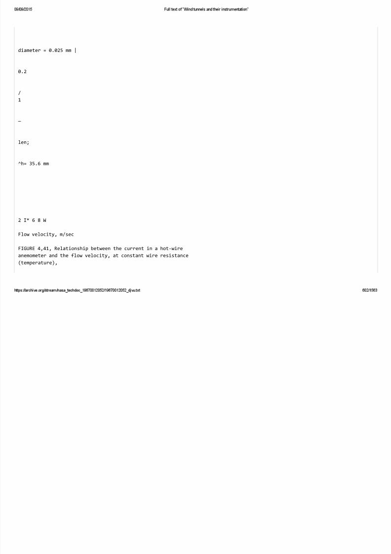
diameter = 0.025 mm |

0.2

/

1

 —

len;

^h= 35.6 mm

2 I* 6 8 W

Flow velocity, m/sec

FIGURE 4,41, Relationship between the current in a hot‐wire

anemometer and the flow velocity, at constant wire resistance

(temperature),

 

the main characteristic of the hot‐wire anemometer, namely its high

sensitivity at low flow velocities. At constant resistance the current

changes with velocity most rapidly at small free ‐stream velocities.

Sensitivity increases with the wire temperature throughout the velocity

range. The temperature of the wire is, however, limited by aging and

strength considerations and should not exceed 400 to 500°C.

If the current through the wire is held constant, the changes in

temperatui'e and resistance of the wire can be predicted. Hot‐wire

anemometers may therefore be used to measure velocity either at constant

resistance or at constant current, as shown in Figure 4.42.

For measurements at constant resistance the wire forms one arm. of

a Wheatstone bridge, the other arms being resistors (e.g., manganin)

193

having a negligible temperature coefficient. A change in the velocity

causes the temperature and resistance of the wire to change; this

unbalances the bridge. In order to restore the balance of the bridge

the wire temperature is restored to its initial value by adjusting the

resistance of the adjacent arm or of an auxiliary resistor (4. 42a).

Velocity is measured in terms of the current in the wire, as indicated,

for instance, by an am.meter connected in an ejcternal circuit.

W 20 SO

 

Velocity, m/sec

bj

®

^

B.5

2.0

''J.5

1.0

[Piatinum wire

<^0.f27mml=Wmu]

'Heating current

|0ai8 amp

 

W 20 30

Velocity, m/sec

FIGURE 4.42. Circuits and calibration curves for hot‐

wire anemometers, a — by the constant‐resistance

method: b — by the constant‐ curreni method.

Higher sensitivity is obtained by a potentiometric method (Figure 4.43)

in which the wire current is determined in terms of the voltage drop across

a constant resistance R having a negligibly small temperature coefficient.

Thus, in the constant‐resistance m.ethod the velocity is determined in terms

of the current (or voltage) needed to maintain a constant temperature, and

thus constant resistance, of the wire.

The circuit for constant‐current measurements is shown in Figure 4.42b.

In this case the velocity is determined from the value of the resistance of

the wire. The current in the wire is adjusted to the required constant value

by means of a rheostat in series with the supply battery. The wire

resistance is measured by a voltmeter of high internal resistance, connected

in parallel. The constant‐resistance method is more widely used, because

it involves simpler measuring equipment. Complex electronic amplifiers

are used to study turbulence.

In recent years, shielded hot‐wire anemometers have been used to

measure low velocities in steady flow (Figure 4.44). A wire heater made

from nichrome (which has a low temperature coefficient of resistance) is

194

 

Hot wire

placed in one of the bores of a twin‐bore ceramic tube of 0.8 to 1 mm

outside diameter ='=. A copper ‐constantan thermocouple in the other bore

serves to measure the temperature of the hot tube. The heater current

is held constant, so that the temperature of the

ceramic tube depends on the flow velocity. By‐

measuring the thermoelectric emS of the thermo‐

couple with a potentiometer or galvometer we can

determine the temperature of the tube, and thus

the flow velocity.

Figure 4. 45 shows a circuit for maintaining a

constant current in the heater wire. An auxiliary

hot‐wire anemometer B, which is an exact replica

of the principal anemometer A, is placed in an

enclosure in which the velocity is zero and the

temperature is constant. The heaters of the

anemonaeters are connected in series. Under

these conditions, the thermal emf Endeveloped

accross the thermocouple of B depends only on the

current / passing through both heaters. A rheostat

R is used to maintain this current constant in

accordance with the indications of the thermo‐

couple B. [For Figures 4.44 and 4. 45 see p. 196. ]

§ 13. THE MEASUREMENT OF FLOW DIRECTION

 

FIGURE 4.43. Potentio‐

metric method for mea‐

suring current in a hot‐

wire anemometer at

constant resistance.

It was mentioned before that the total‐ and

static ‐pressure readings by tubes are affected by

the flow direction. The best instruments are,

therefore, those which depend least on yaw.

Exactly the contrary is true for tubes which are

used for measuring the flow direction.

Usually yawmeters also measure other flow characteristics. An ideal

tube would be suitable for measuring independently four quantities: the

angles a. and 3 of the inclination of the three‐dimensional flow to two

mutually perpendicular planes, the total pressure p„ , and static pressure f

The first pair of measurements determines the directions, and the second,

the magnitude, of the velocity vector.

All‐purpose tubes of this kind find wide application in investigations

of turbomachines. They are, however, less accurate than dual‐purpose

tubes in the measurement of the magnitude of the velocity vector, due to

the difficulty of measuring the static pressure accurately.

Pressure‐sensing instruments for measuring the flow direction can

be divided into two groups. The first group consists of devices in which

the yaw is measured in terms of the pressure difference between two

tubes whose orifices are arranged at a fixed angle with respect to each

other.

 

[Simmons, I.. F. G. A Shielded Hot‐wire Anemometer for Low Speeds. — J. S. I. Vol. 26, p. 407. 1949. ]

195

A total ‐pressure tube cut at a right angle to its axis is not

very sensitive to variations of the yaw angle a between its axis

Thermocouple

(copper‐ consranian)

therm'

r

Auxiliary j |l||

Tioanemometerl B

 

't>r‐3.

Enclosure

SaMV

To the galvanometer (/

Principal

thetmoanemometer A

FIGURE 4. 44. Shielded hot‐wire anemometer.

FIGURE 4.45. Circuit diagram of shielded

hot‐wire anemometer.

and the flow direction when a is less than 15 to 20°. The sensitivity

increases sharply when a is between 40° and 60°; if the tube is cut at an

angle to its axis, the same order of sensitivity can be obtained /3/ when

 

a = F gure 4.46 .

FIGURE 4.46. Variation with angle « of the difference between

the pressure in the tube and the static pressure in the flow for plot

tubes faced off at various angles 9.

196

The second group includes devices based on measuring the pressure

difference between two points on the surface of a streamlined symmetrical

body (sphere, cylinder, wedge, or cone). When the axis (or the plane of

symmetry) of the body coincides with the direction of flow, the pressure

at symmetrically located points is equal.

The orifices are situated on the body (or the direction of the tubes is

chosen) in such a way that small changes in flow direction cause large

pressure differences between the orifices which are connected to a

differential manometer.

The sensitivity p( of the tube is determined by the change in pressure at

one of the orifices, due to a change in yaw:

dp , ‐ p—p

The sensitivity is thus defined as the slope of the tangent to the curve

p = /(a) The pressure at an orifice in a circular cylinder, whose axis is

perpendicular to the flow, is most affected by the flow direction if the

 

rad us through the or f ce makes an angle of 40 to 50° w th the flow

direction (see Figure 4.4).

A differential manometer connected to the yawmeter measures the

pressure difference between two such orifices (1 and 2) so that the

true sensitivity of the nozzle

<%

Pi'

da

must be twice the value of dp/dn, obtained from the slope of the curves in

Figure 4.4. The value of k varies between 0.04 and 0,08 per degree for

different types of tubes.

The yawmeters are sensitive to transverse velocity gradients, which

cause the pressures at two points situated symmetrically about the axis of

the tube to be unequal, even when the tube axis coincides with the direction

of flow. In this case the pressure difference between the orifices is zero

at an angle which depends on the magnitude of the gradient, the distance

between the orifices, their size, and the sensitivity of the tube [to pressure

changes]. The best method to reduce the error due to transverse velocity

gradients is to decrease the distance between the orifices. This, however,

causes a decrease in the diameter of the orifices and of the tubes between

the orifices and the manometer, which, in turn, increases the lag of the

manometer indications because of the high flow impedance of the tubes.

 

Th s should be taken nto account when choos ng the tube and manometer.

Yawmeters can be used directly or as null instruments. In the null

method the yawmeter is rotated on a cradle until its axis coincides with

the direction of the flow, as indicated by zero pressure difference in the

differential manometer connected to the orifices. The direction of flow

is then indicated by graduations on the cradle.

In the direct method the tube is held at a constant angle to the tunnel

wall, and the yaw is determined in terms of the pressure drop between the

orifices, measured by a differential manometer. The relationship between

yaw and manometer indication is established by calibrating the tube in a

wind tunnel of negligibly small transverse velocity gradients and flow

197

inclination. The direct measuring method requires less complicated

equipment and less time than the null method, but is less accurate,

especially at large angles of yaw. Because of its simplicity, and because

it is possible to obtain simultaneous readings from an array of tubes, the

direct method is usually employed in the calibration of wind tunnels, where

normally the flow inclination is small. In the direct method the tubes can

be easily adapted for measuring the velocity and direction of the flow in two

planes.

The advantage of the null method of yaw measurement lies in the

independence of the measurements on M and Re. It is also less important

to locate the orifices very accurately on the tube in this method, since their

positions merely affect the relationship between yaw and pressure drop.

The null method is usually chosen for measuring flow angles in wakes, e. g.,

 

n exper ments w th blade cascades.

The combination of a direct and a null method is sometimes used in

studying three‐dimensional flow.

p,', h'>.

'0'

c)

FIGURE 4. 47. Tubular yavv'incters cut ar right angles, a and b —for Iwo‐dimenstona] flow;

c — for three‐dimensional flow.

Tubular yawmeters shown in Figure 4. 47 consist of coplanar bent tubes,

with ends cut at right angles, inclined to each other at an angle of 90°. The

tube in Figure 4.47c is intended for three‐dimensional flow. The angle of

flow inclination in the a‐,? plane can be measured by the null method (by

rotating the tube about the y axis until the pressures in orifices 1 and 3 are

equal), while the angle of inclination in the xy plane is found by the direct

method in terms of the pressures difference between tubes 4 and 5, For

 

measur ng the flow veloc ty, yawmeters of th s type are equ pped w th the

additional tube 2, which senses the total pressure. The flow velocity can be

determined from the pressure difference between the orifices of this tube

and one of the lateral tubes, if the tube is calibrated against a

reference dual‐purpose tube. The drawback of these tubes is their

low rigidity. Small deformations of the tubes can cause considerable errors

when measuring yaw.

198

Recently, tubular yawmeters with beveled ends are increasingly being

used for the study of blade cascades. Such tubes have external diameters

of 0.5 to 2 mm. The tubes are mounted parallel to each other, so that the

distance between their orifices is very small. In two‐dimensional flow

the influence of velocity gradients can be almost completely eliminated by

locating the tube axes not in the plane of flow inclination but in a plane

perpendicular to it, as shown in Figure 4.48d.

Figure 4.46 shows that in order to obtain maximum sensitivity to yaw,

the tubes should be cut at an angle between 30 and 45°. Figure 4.48a gives

the sensitivity characteristics of a two‐tube yawmeter designed for small

flow velocities. The characteristics of three ‐tube yawmeters for the

direct method of measurement are usually expressed as a graph showing x^

as a function of a , where

^ Pi — Pz

(Pi — Pi) + (Pi — Pi)

 

Figure 4.48b shows the variation of n.^ with a for three‐tube yawmeters of

various bevel angles ip.

At small flow velocities (up to M = 0.3 to 0.4) a beveled‐tube yawmeter

can be used for the measurment of both direction and speed. The total and

static pressures can be determined with a two‐tube yawmeter (4. 48a),

for example, by the following method: the yawmeter is turned until the

pressures in tubes 1 and 2 are equal (pi = ps = p'). The values of p, and pj are

then determined after further rotation of the tube by angles of ±10°. The

total and static pressures are then found with the aid of experimentally

determined calibration coefficients k, and Aj /13/,

/'o = P' + *A

p=p' + k^^,

where

A = 4‐ {(Pi) , w ‐ (P2) , ,0" — (/'i>‐ .0‐ + (/'2)‐io'l >

whence

The yawmeter shown in Figure 4. 48b is fitted with a central tube 2 for

measuring the total pressure po, which can be determined by adjusting the

tube so that pi = P3 = p' . The flow velocity can be found with the aid of the

coefficient 5^, :

t _ ? p« :^p_

 

''' 2 p,‐p' ~ 2 p,‐p' •

which is also determined by calibration against a reference tube.

Figure 4.48c shows the design of a four‐tube yawmeter for three‐

dimensional flow measurements. The yawmeter consists of tubes whose

outside and inside diameters are 0.8 mm and 0.5 mm respectively; the

199

^^

 

•\\

\^

«^

tt

^v

 

^

is

^

^

‐

‐

 

5:

i:

"^

 

s

>4

H («3 ^ ^ ^

C=‐ « ■=6‐ =

3

y csj ^ to oo c:^

^3 Ca‐ ca <^ ‐^

 

op

iS'

^

^

1

‐

\

 —

 

‐

 

_

_

_\

^

200

tubes are connected at the nose, and cut at 45°. The characteristics of

this tube for M= 1.86 and 2.67 are shown in the same figure /14/. The

sensitivity to yaw of such tubes is similar to that of wedges (Figure 4.53)

and other types of yawmeter for supersonic velocities.

Cylindrical yawmeters

Cylindrical yawmeters (Figure 4.49) are used for determining the

 

direction of two‐dimensional flow. As can be seen from the characteristics

shown in Figure 4. 49b, their sensitivity is highest when the included angle

2‐[ between orifices (1) and (3) is between 90 and 100°. A third orifice, for

m.easuring the total pressure, is drilled in the center between the two yaw‐

meter orifices. Cylindrical yawmeters are generally used for the null

method; the total pressure is measured when the pressures at the outer

orifices are equal. The flow velocity can thus be determined from the pressure

difference between the central and one of the outer orifices, provided

that the velocity‐calibration coefficient J,‐ is known; it is determined in

the same way as for multiple ‐tube yawmeters. The value of Iv depends

on the flow regime around the tube. The pressure at the front of the

cylinder may differ from the theoretical value for potential flow (see

Figure 4.4) because of boundary‐layer separation. If boundary‐layer

separation takes place symmetrically on the upper and lower surfaces

of the front quadrants of the cylinder, the change of pressure at the wall,

due to the consequent change in Reynolds number , will not affect the yaw

calibration coefficient x„, but there may be a considerable change in the

velocity‐calibration coefficient Iv . Figure 4.49c shows that x^ is virtually

independent of Re, and is directly proportional to the yaw angle a for values

below 15°, Nevertheless, the cylindrical yawmeter should be used with

caution at M>0,6, since local asymmetrical shocks may appear. The

velocity coefficient iv begins to be affected by compressibility at A. » 0.3

as can be seen from the graph of Figure 4. 49d.

The advantage of the cylindrical yawmeter over other types is its small

diameter, since it occupies an area, perpendicular to the flow, determined

merely by the outside diameter of the tube, which can be very small. This

is important, e. g., when investigating the flow between stator and rotor

blades of axial turbomachines. Tubes with outside diameters up to 2.5 or

3 mm are used for blade‐cascade investigations.

Spherical yawmeters

 

Spherical yawmeters (Figure 4, 50) permit flow‐direction measurements

in three‐dimensional flow with the aid of four orifices located in pairs in

two mutually perpendicular planes, A fifth opening, at the intersection of

these planes, serves for measuring the total pressure. The determination

of the direction of a three‐dimensional flow by the null method requires

the use of a complicated cradle giving indications of the angular position in

two planes. Only the angle g, in the Aryplane, is therefore measured by

201

r

‐^

^

^

 

 —

s:

^

^

:^

5'

^

\

 

202

the null method; the angle a in a plane perpendicular to the xy plane Is

determined by the direct method with the aid of a calibration curve obtained

by two‐dimensional flow tests (Figure 4. 50).

‐2.0

PrPs

‐1.2

OS

‐0.4

A _

S W IS

Bevel ingle a: •

 

20 25

FIGURK ‐1. .^)0, Splierical yavvineter and its cliaracteristics

(!iicliidt.‐d angle btluuen orifices is '.*0°"t.

When the yawmeter cannot be turned (e. g., when it is mounted on a

turbine rotor) we can measure both angles directly with an accuracy of

± 1 to 2", while simultaneously measuring the velocity and static pressure

with an accuracy of the order of ±3% /I 5/.

The drawback of spherical yawmeters is the limited range of Reynolds

numbers (from. 4X10^ to 1.5X10^) within which their calibration coefficients

are constant. When the laminar boundary layer becomes turbulant, the

point of flow separation on the surface of the sphere becomes indeterminate;

the flow around the sphere becomes asymmetrical, and this causes

inaccuracies in measurement.

Hemispherical yawmeters

If we replace the rear half of the sphere by a cylinder, the flow

conditions are improved and the point of boundary‐layer separation is

removed from the neighborhood of the orifices. Hemispherical yaw‐

meters have the same sensitivity as spherical ones, but the influence

 

203

of the Reynolds number on their characteristics is much smaller. The

sensitivity of hemispherical yawm.eters decreases at large Mach numbers.

Figure 4. 51 shows the TsAGI six‐bore yawmeter /22/. In addition

to the five openings in the hemispherical nose for measuring total pressure

and flow direction, the yawmeter has an opening on its cylindrical stem

for measuring the static pressure.

FIGURE 4.51. TsAGI six‐ bore yawmeter.

The TsAGI yawmeter is used for determining the magnitude and

direction of the flow velocity in subsonic wind tunnels. The flow

inclination in wind tunnels is generally small, so that the measurenaents

are made by the direct method, i, e,, without rotating the yawmeter. By

calibrating [the yawmeter] in a wind tunnel in which the flow inclination is

very small, we obtain

Pi—Pz

T=/K

 

(.Pi — P2) + (Pi — P2)

(P,‐P2) + (P,‐P2) ^^^''

where pi, ps and P4, ps are the pressures in the orifices located in the vertical and

horizontal planes respectively. At small yaw angles the yaw measurements

in one plane are independent of the yaw in the other. Corrections must,

however, be made when the yaw exceeds 5°, and these are determined by

calibration as o = /(a)and « = f(^).

Wedge‐type and conical yawmeters

Wedge‐type yawmeters (Figure 4. 52) can be used for measuring the

flow inclination at velocities above those at which shocks appear on the

surface of a sphere or cylinder, i. e. , at M > 0.55 to 0.6 /1 6/. The

advantage of these over cylindrical yawmeters is that the position of the

orifices on the surface is less critical. The pressure‐distribution curves

204

in Figure 4. 52 show that with wedge‐type yawmeters the pressure

measurement is far less sensitive to the location of the orifices than

with cylindrical yawmeters, so that manufacturing tolerances can be far

wider. Either a separate orifice on the leading edge of the wedge, or a

 

FIGURE 4, 52. Wedge‐type yawmeter and its characteristics (the pressure

distribution on the surface of a cylindrical yawmeter is shown for comparison).

completely separate tube, can be used for measuring the total pressure.

Wedge‐type yawmeters can be used to measure the static pressure at

higher Mach numbers than cylindrical yawmeters.

O.IS

OJO

0.05

‐0B5

‐0.W

‐0.15

‐^

 

‐s

^

PrPi

!S

■^

^

^

■

(^

 

J

'^'

^*

H.

%

mm W. G.

500

250

‐250

■500

 

‐J*

At n'lk.p.‐is

r z‐

Yaw angle of the wedge

■M‐/.«

FIGURE 4. 53. Wedge‐type yawmeter for measuring

the direction of supersonic flow.

205

Wedge‐type and conical yawmeters with small included angles are

among the most reliable instruments for investigating supersonic

flow. Figure 4. 53 shows the characteristic of a wedge‐type yawmeter

designed by the NAE Laboratory (Great Britain) for calibrating the

 

0.9 mXO.9 m test sect on of a cont nuous‐ operat dn superson c w nd tunnel / 17/.

The wedge yawmeter is installed on

a spherical cradle so that it can be

used for null‐method measurenaents

of the flow inclination.

Figure 4. 54 shows the character‐

istics of conical and pyramidal RAE

yawmeters for the direct‐method

measurement in three‐dimensional

supersonic flow. The sensitivity of

A^‐ ^"^ b) >» y' conical yawmeters increases with the

^J J‐f Jy^ Vp cone angle, but an included angle of

15° provides sufficient sensitivity,

since an error of 1 ram W.G. in the

naeasured pressure causes an error

of only 0.02° in the yaw determination.

Yawmeters can therefore be designed

with other (e.g., production)

considerations in mind. If the nose is

pyramidal (Figure 4. 54c) the exact

location of the orifices is much less

critical than for circular cones (where

they m.ust lie exactly in two mutually

perpendicular planes) because flow

round a pyramid is much less precisely

defined. The calibration curves for

these yawnaeters rem.ain linear even

when the shock has become detached.

All measurements in a series must, however, be carried out with the shock

either attached or detached, since the calibration differs in these two

 

cases / 18/.

FIGURE 4.54. Characteristics of yawmeters for

three‐dimensional supersonic flow, a and b —

conical yawmeters; c — pyramidal yawmeters .

Heated wires

Galvanometer

FIGURE 4. 55. Hot‐wire yawmeters .

206

Measurements of flow direction with

a hot‐wire yawmeter

If two identical wires arl heated by the same current and placed in

a uniform flow parallel to their plane, their rates of cooling will

 

d ffer unless they are ncl ned at the same angles to the flow d rect on.

Hot‐wire yawmeters function on this principle. The wires are stretched

between manganin posts A, B , and C (Figure 4. 55) so as to include an angle

p, and are connected to adjacent arms of aWheatstone bridge. The instrument

is rotated about an axis perpendicular both to the flow and to the plane of

the wires, until both wires are at the same temperature and have the same

resistance, so that the Wheatstone bridge is balanced. The flow direction

is then parallel to a line bisecting the angle p. Since the dimensions and

the electrical characteristics of the wires may differ, the instrument must

be calibrated in a wind tunnel where the flow direction is known.

§ 14. MEASUREMENT OF TEMPERATURE IN FLOW

The measurement of the temperature of a flowing gas is important in

investigations of the aerodynamic heating of the surfaces of aircraft and

rockets, and in studies of the operation of gas turbines, compressors,

aircraft engines, etc.

The state of a stationary perfect gas can be defined by two independent

physical magnitudes, one of which may be the temperature. If the flow

velocity is such that compressibility effects are important it is necessary

to differentiate between the static temperature T and the stagnation (total)

temperature 7"o . A thermometer moving with the fluid, and emitting no

thermal radiation would measure the static temperature. In practice the

static temperature can be determined only indirectly, for instance by

measuring the static pressure with a tube and the density optically, and

then using (4. 1); or by measuring the velocity of sound a and using (4.3a).

Measurements of the velocity of sound in a moving medium must be

corrected for the flow velocity. Both electronic and optical methods are used

for these measurements, but only a mean temperature within a certain region

can be determined thus, so that this method is seldom used. It is much simpler

 

to determ ne the temperature T by measur ng the stagnat on temperature

and the Mach number. The stagnation temperature is the temperature which

the gas would attain if brought to rest adiabatically, so that its entire kinetic

energy is transformed without loss into heat. This temperature would be

shown by a thermometer placed at the stagnation point of a body in the

stream, provided no heat is lost to the surrounding medium. However, it

is virtually impossible to make a thermometer which loses no heat at all.

Furthermore, it would always have finite dimensions and thus cause

turbulence, thus changing the local temperature. A thermometer

inserted into a fast‐flowing gas will therefore indicate a temperature

lying between the static and the stagnation temperatures.

The difference between the stagnation temperature To and the true

temperature T of a moving perfect gas (in which temperature changes

207

are adiabatic) can be determined from

T,~T =

2,?/c/ «

Since shocks do not affect the enthalpy of a gas, this equation is true both

for subsonic and supersonic flow.

 

A thermally nsulated surface w ll be heated by a gas flow ng past t

to a temperature called the recovery temperature Ta . The recovery

temperature depends on the local Mach number (or on the static temperature)

at the outside limit of the boundary layer, on the dissipation of kinetic

energy by friction in the boundary layer, and on the rate of heat exchange.

The difference between the recovery temperature and the static

temperature is a fraction r of the adiabatic temperature rise:

^'.‐^ = '‐2i^‐ (4.48)

The coefficient r, called the coefficient of thermal recovery, is defined by

/‐ = ^^. (4.49)

In general the coefficient of thermal recovery, which represents the

proportion of the kinetic energy of the medium recovered as heat, depends

on the shape of the body, and on M, Re, Pr and x. For a given gas, Pr and x

are constant over a wide range of the temperatures usual in subsonic and

supersonic wind tunnels (for air, Pr = 0.72, x = 1‐4 ) and we can thus consider

r as a function of M and Re only. The value of r may vary over the surface.

For laminar flow of an incompressible fluid around a flat plate, r depends

only on the rate of heat exchange and the friction in the boundary layer on

the surface of the plate. When Pr = 1, heat exchange and frictional heating

compensate each other, and the adiabatic temiperature on the surface is

equal to the stagnation temperature To , i. e., r = 1.

Theoretically the recovery coefficient in laminar and turbulent boundary

layers at a flat plate should be /• = Pr''» and r = Pr''' respectively, but

experimental values of 0.85 and 0.89 respectively, have been obtained.

The coefficient of thermal recovery depends on the shape of the surface.

Studies in supersonic wind tunnels have shown that for poorly streamlined

 

bod es r var es between 0,6 and 0.7, and for well streaml ned bod es,

between 0,8 and 0.9.

The relationship between the recovery temperature and the stagnation

temperature depends on the Mach number, and can be deduced from (4.4)

and (4.49):

‐^=1 Izrr (!‐'•)• (4.50)

This function is plotted for x = 1.4 and various values of r in Figure 4. 56.

In subsonic flow T„ decreases with increasing velocity. When M exceeds

unity, a shock appears upstream of the body whose leading edge is

therefore in a subsonic region; hence, the Mach number in (4. 50) is less

208

than unity. With increasing supersonic free‐stream velocity, the strength

of the shock increases, the Mach number decreases, and therefore the

value of Ta rises.

In the absence of heat transfer, a thermometer on the wall of a tube

inserted into a gas stream would indicate a recovery temperature Ta

dependent only on the flow characteristics in the boundary layer around

the tube. When r= \.0,Ta= To‐ However, an actual thermometer, in which

heat exchange with the surrounding medium cannot be prevented, will

indicate a temperature Tn differing from the recovery temperature '/'„.

The principal characteristic of a thermometer is therefore the

dimensionless quantity

 

T‐n‐T‐

(4.51)

which is called the recovery coefficient of the instrument. By definition,

the recovery coefficient C, allows for the effects of heat exchange between

the thermometer and the surrounding atmosphere caused by the heat

conductivity of the instrument holder and by heat radiation.

The value of ^ for a given instrument can be established experimentally

by calibration in a special wind tunnel. Knowing the temperature Tn, as

measured by the instrument, and its recovery coefficient g, we can

determine the stagnation temperature T„, by substituting Ta and r for T^

and 5 in (4. 50).

t.O 1.5 2.0 2.S 3.0

Free‐stream Mach number (upstream of the shock)

1.0

 

O.WI 0.577 0.513 0.475

Mach number do‐wnstream of the shock

FIGURE 4. 56. Ratio TJT^ as a function of the Mach number for a thermometer

of finite dimensions in subsonic flow, and in supersonic How vvith a shock.

209

lllllllllllllllllllllllllllllllllllllllllllllllllllllllllll Mini

II II lllllllllll III lllllllll lllllll

nil III

Sensors for measuring stagnation temperature

The design of a temperature sensor depends on the intended range of flow

velocities and temperatures. The design and naaterial of the sensor can be

so chosen that it will indicate a temperature 7"n which is sufficiently close to

the stagnation temperature of the flow. Such a sensor can be called a

stagnation‐temperature sensor.

 

For a good stagnation‐temperature sensor, the value of ^ should be close

to unity. However, it is even more important that J should be constant,

or change very little over the relevant range of velocities and temperatures.

The deviation from unity of the value of 5 depends on: 1) convectional

heat exchange between sensing element and medium; 2) heat loss by

conduction from the sensor through the device holding it; 3) radiant‐heat

exchange between sensor and the surroundings.

Since the processes by which heat exchange takes place vary with flow

velocity and temperature, the design of the sensor depends on the values

within the test range of all the physical parameters. Sensors can be

roughly divided into three groups depending on the range of measurements:

1) sensors for low and high velocities at lowtemperatures; 2) sensorsfor high

velocities, and temperatures up to 300 and 400°C; 3) sensors for low and

high velocities at high temperatures (up to 1000 — 1200°C).

Low‐temperature sensors. The effect of [heat] radiation can be

neglected if the temperature of the wall on which the sensor is raounted

differs very little from the temperature of the flowing medium. To

determine the latter in the test section of most wind tunnels (for low or

high velocities) it is sufficient to measure the stagnation temperature in the

settling chamber of the tunnel. Since there is practically no input or removal of

heat between the settling chamber and the test section, the stagnation

temperature remains constant. The flow velocity in the settling chamber

does not usually exceed some tens of m/sec and the temperature,

some tens of degrees centigrade.

Mercury thermometers can be used as sensing elements in this range,

but resistance thermometers and thermocouples provide faster operation

and permit remote indication. The design of a resistance thermometer for

measuring temperatures in the settling chamber of a wind tunnel is shown in

Figure 4. 57. The change in the resistance of the wire, as a function of

 

temperature, can be measured w th the a d of a rat ometer or a Wheat‐

stone bridge. If all other parameters in a wind tunnel or on a test bench

are measured and recorded automatically, it is better to use the automatic

electronic bridges (currently made by Soviet industry). Standard bridges

have usually a recording or indicating device actuated by a balancing motor

placed inside the instrument. For automatic recording of temperature together

with other parameters the balancing motor of the bridge is connected to a

recorder or printer by means of a Selsyn or a digital converter (see

Chapter DC). Automatic bridges permit the temperature to be measured

to an accuracy of tenths of a degree.

Sensors for high velocities and medium temperatures.

When testing compressors it is necessary to measure temperatures up to

3 00° Or 400°C at up to sonic velocities. The same range of stagnation

temperature is found in supersonic wind tunnels fitted with air heating

and in tunnels for heat‐exchange tests. In most cases the sensors are

210

mounted in relatively narrow channels; in order to reduce the disturbances

caused by them, the sensors should be small, for which the best sensing

element is a thermocouple with wires of 0.1 to 0.2mm diameter. For the

range of temperatures considered iron‐constantan or copper‐constantan

therraocouples are generally employed; they have sensitivities of 5 and

4 millivolts per 100°C respectively. The thermal capacity of the junction

of the thermocouple is very small, so that it responds rapidly and

measurement can be made at rapidly changing temperatures.

 

empera ure

sensor

Frame made of insulating

material

Copper

spiral

Electronic

bridge

console

FIGURE 4. 57. Resistance thertjiometer

for measuring the temperature in the

settling‐chainber of a wind tunnel.

FIGURE 4. 58. Rt‐sisrance thcnnotuctcT tor

measuring the temperature ui the settling‐

chamber of a wind tuiinei.

 

When there is no radiant‐heat exchange, a thermocouple consisting of

butt‐welded copper and constantan wires, inserted lengthwise into the

flowing medium, will have a stable recovery coefficient [T, = 0.9) for

0,2 < M < 1,0 and 3.8‐ 10^ <Re<14.4‐ lO^. The value of ^ is not constant for a

thermocouple inserted transversely, since the recovery coefficient increases

with velocity /1 9/. Although t, is constant for bare wires inserted length‐

wise, temperature sensors of this type are not widely used because of

manufacturing difficulties .

Attempts have been made to measure the stagnation temperature with

thermocouples installed at the frontal stagnation point of a streamlined

sensor. It was found possible in such sensors to achieve a balance between

heat exchange by convection with the medium and heat exchange by conduction

with the supports. However, this type of sensor is very sensitive to slight

changes in its shape, yaw, and radiant‐heat exchange, and is not widely used

The most reliable design of stagnation‐temperature sensors, having

recovery coefficients close to unity over a wide range of velocities, relies

on bringing the fluid to rest adiabatically near the thermocouple junction.

211

The gas upstream of the junction can be slowed down to a certain optimum

velocity, where heat gained by the junction due to thermal convection in the

gas is balanced by the heat lost from the junction due to the heat conduction of the

supports. In low‐ velocity flow the temperature and velocity gradients are

small, so that heat exchange and friction in the boundary layer at the junction

of the thermocouple are insignificant. The medium is brought to rest adiabati‐

cally in a total‐ pressure tube, and the best temperature sensors so far developed

 

are based on such tubes of mod f ed shape. A further advantage of th s

design is that the tube can also be used as a radiation shield to prevent

radiant‐heat exchange with the surrounding medium. In order to prevent

the gas from coming to rest completely, and to maintain a certain convective

heat transfer to the junction in order to balance the loss through thermal

conduction, the tube has outlet orifices whose area is 1/4 to 1/8 of the area

of the inlet orifice. The dimensions and shape of a sensor within the

stagnation zone inside a tube are less critical, and naeasurement

reproducibility is better than if the thernnometer were placed on the surface,

where the recovery coefficient would depend on the flow conditions around

the body. Thus, it has been possible to design sensors with recovery

coefficients of the order of 0.99 for 0.2 < M < 3.0.

0.98

ass

OM

0.32

312m/

sec

 

5^

y^^

m

180

129

 

‐80' ‐W W 20'

Yaw angle

150 300 m/sec

Free‐stream velocity

FIGURE 4. 59. Section and characteristics of the Pratt and

and Whitney Pitot thermocouple .

212

In one of the earliest designs of shielded temperature sensors used at

high velocities, the thermocouple was placed in the stagnation chamber

of a round‐nosed tube. Air entered into the chamber through a diffuser

and small ventilating holes were drilled in the chamber walls to make up

the heat losses from, conduction and radiation. Figure 4.58 shows the design

and characteristics of a sensor of this type, having an external diameter

of 4.7mm [20]. Such a sensor is highly sensitive to yaw; there is a large,

random error in its calibration curve, caused by flow instability in the

diffuser. The reason for the abrupt change in recovery coefficient at a velocity

of about 90 m/ sec is the transition from laminar to turbulent flow at the

diffuser inlet, where Re = 2000 to 3000.

 

Subsequent investigations of Pitot thermocouples have shown that better

reproducibility and reduced sensitivity to yaw is obtained by placing the

thermocouple in a cylindrical stagnation chamber. Figure 4. 59 shows the

design and characteristics of such a sensor. These sensors are very

widely used because of their simple design. Their recovery coefficients

vary between 0.95 and 0.999.

Aluminum

'0**‐

1

FIGURE 4.60. Double‐shielded Pitot thermocouple.

Figure 4.60 shows the sensor designed at the Swedish Royal Technological

Institute. It has a recovery coefficient very close to unity. The thermo‐

couple junction, 0.15 mm in diameter and made from iron‐constantan ,

is surrounded by two aluminum tubes, joined at the nose of the sensor by

means of heat ‐insulating material. At zero yaw the recovery coefficients

of round‐ and conical‐nosed instruments of this type are 0.998 and 0.996

 

213

respectively. Yaws of 5 to 10° have practically no effect on the recovery

coefficients, which have also been found to remain practically constant at

temperatures of up to 250''C /21/.

Sensors for measuring the stagnation temperatures between the stages

of turbocompressors and gas turbines must be as small as possible both

in diameter and length. The designs of two such instruments are shown in

Figures 4. 61 and 4, 62.

Boundary‐layer temperature measurements are made with miniature

instruments, similar to that shown in Figure 4. 59. Medical hypodermic

needles, whose diameters are fractions of millimeters, are used for the

external tubes.

The value of J tends to decrease at low velocities, at which heat input

by convection to the thermocouple no longer balances losses by conduction

through the supports.

High‐temperature sensors

For high temperatures (above 3 00° or 400°C), at which the temperature

difference between the sensor and the surrounding m.edium is of the order

of 50°C or more, radiant‐heat losses become the principal source of error.

 

Exact measurements of stagnation temperatures

are very difficult in this range, where even slight

changes in ambient temperature lead to considerable

changes in the temperature of the sensor.

The amount of heat lost by radiation is

proportional to the surface area of the sensor,

so that for high‐tenaperature duty, sensors should

be as small as is consistent with strength

requirements. The radiation capacity of the surface

of the body on which the sensor is mounted should

also be very low: this can be achieved, for instance,

by polishing the surface. It is difficult, however, to

avoid gradual oxidation of the surface of a sensor

immersed in hot gases. The best method of reducing

radiation is to improve the shielding of the sensor.

The thermocouple of the sensor is mounted in a

diffuser surrounded by several concentric

tubular screens ( Figure 4. 63 ). The external

screens are heated by the gas flowing through

the annular gaps. The thermocouple junction

may be either mounted in the middle of the central

tube or welded to it. In the first case the

recovery coefficient of the sensor is similar to

that of a poorly streamlined body (I » 0.65). In the second case, the value

of the recovery coefficient approaches that of a flat plate {t, ~ 0.9). Good

results have been obtained at temperatures up to 900 to 1000°C with

chromel‐alumel thermocouples miounted in enclosures of the above described

type. The inner screen may be made of porcelain, and the three outer

screens of heat‐resistant steel.

 

FIGURE 4. 61. Cylindrical

temperature sensor

( M = 1 , c = 0. 98) .

214

Radiation losses in high‐temperature sensors can be reduced by heating

the shield to a temperature close to the ambient temperature of the medium.

1.02

1.00

ass

0.96

094

t

1.02

 

:

^

‐

.

 —

■ —

 

60

120

WO 240

V, m/sec

^ 1.00

‐^0.93

096

 

0.94

0.92

/■

r

‐ar

^

 

^

^‐P

cc‐

V

\

 

‐40‐ ‐20'

20' 40'

FIGURE 4. 62. Cylindrical temperature sensor with

open mlet.

Figure 4. 64 shows the design of a miniature stagnation ‐temperature sensor

developed by the California Institute of Technology /23/. In this sensor,

an electrically heated wire on the shield reduces direct radiation losses

and losses by heat conduction from the shield. To compensate for heat

losses by conduction through the leads from the thermocouple and its holder,

the latter is heated by a separate nichrome resistor heater. The

temperatures of the shield 7"s and of the holder fi, are measured by separate

 

thermocouples, and controlled to be as nearly as poss ble equal to the

215

temperature ?"„ of the main thermocouple. Figure 4.65 shows the values of the

recovery coefficients Ss‐Eh‐ ^^'^ ^ obtained by inserting the corresponding

FIGURE 4. 63. Shielded sensor for high temperatures.

FIGURE 4. 64. Temperature sensor with heated shield.

1— main thermocouple mounting and heating element;

2— radiation shield and heating element.

Re W*

FIGURE 4. 65. Characteristics of a temperature sensor with heated shield and

holder (M = 5.75).

 

values of T^, T^ and 7"n into (4. 51). In the absence of heating, t,^ and J

depend on boththe Reynolds number and the stagnation temperature To .

216

If we heat the thermocouple holder in such a way that7"i, = T^ , i. e., if we

eliminate the heat losses due to conduction, then the recovery coefficient

?n=?h will be higher. If both the holder and the shield are heated, so that

7"l, = 7*5 = Tn, there will be no temperature gradients and the temperature of

the main thermocouple will be exactly equal to the stagnation temperature

(5=1)‐

Calibration of temperature sensors

Figure 4. 66 shows a wind‐tunnel layout for the calibration of temperature

sensors. The air from the compressor is cleaned in oil ‐filled air filters, and

after suitable cooling is led into a vertical chamber, whose upper part is a

smoothly tapering cone with asmallcylindricalportthrough which the air is

ejected to the atmosphere. The chamber is placed vertically in order to

avoid flow asymmetry due to convection.

FIGURE 4, 66. Installation for calibrating temperature sensors.

1 —wind tunnel; 2 —compressor; 3 —receiver, cooler and

 

f lter; 4 —rad at on sh eld and heater; 5 ‐a r heater; 6 —

sensor being calibrated; 7 ‐stagnation‐temperature sensor;

8 ‐total‐pressure tube; 9 —potentiometer.

The stagriation ‐temperature sensor (6) to be calibrated is mounted above

the outlet port. Another stagnation‐temperature sensor (7) and a total‐

pressure tube (8) are installed at the center of the chamber, where the flow

velocity is small. Assuming that there are no energy losses by friction and

heat transfer, the stagnation temperature and the total pressure must have

217

equal values at the outlet and in the centre of the chamber. The walls of

the port are lagged in order to reduce heat exchange through them.

Radiation effects are studied using an electrically heated radiation

shield (4). A further electrical heater (5) is provided at the wind‐tunnel

inlet, for studying the performance of the sensor at high temperatures.

The cold junctions of the thermocouples are brought out to ice‐water

baths placed close to the lead‐through of each sensor. The thermal emf

of the sensors is measured with a high‐accuracy potentiometer connected

to a center ‐zero galvanometer. Temperatures can be measured with an

accuracy of 0.05°C at a galvanometer sensitivity of 10"^ amps.

The proportionality constants k, and k2 of emf versus temperature

for the thermocouples in the reference sensor and the sensor being

calibrated are determined beforehand by static calibration against a standard

thermometer.

 

e ore eac es , e sensor o e ca ra e s moun e n e c am er nex

to the reference sensor in steady flow conditions . The difference between the

indications (thermal emfs of the sensors, in this case at the same

temperature to ) is due only to the difference Af between their calibration

coefficients. This difference

\U=U,‐U, = ^

^0 ^

is measured by the differential method. The sensor being calibrated is then

placed at the outlet port. The indication of the reference sensor remains

unchanged, being U, = ‐^. The indication of the sensor being calibrated will

have the new value 6^2 = ‐7r 'where t„ is the corresponding temperature, which

depends on the recovery coefficient t,. The difference between the

indications of the two sensors, measured by the differential method, is

A6f ' = i/, — i/,'= A — 4a‐ .

We can thus determine the true temperature difference between the two

sensors :

A6f ; — Ai/ = £72 — i/2 = ‐^^^ ,

This method has the advantage of measuring the small differences AU

 

and A l' so that the cal brat on errors are much smaller than f the

thermal emf of each thermocouple were measured separately.

The recovery coefficient can be found from

2gJc„

where the flow velocity is determined by measuring the total

stagnation temperature in the settling chamber.

1680

218

§ 15. MEASUREMENT OF DENSITY:

HUMIDITY CORRECTIONS

The density of a perfect gas can be determined from the equation of

state (4. 1). For air at S.T.P. U = 15°C, p = 10,331 kg/m^ or B,5 = 760 mm Hg,

S = 9.81 m/sec^, R = 29.27 m/ degree) we have

p.3 = 0.125i^.

To calculate the density of air for other conditions we use the concept

of relative density

 

Inserting into this the value for the density determined from the equation of

state, we obtain

A — ZZlL— B( 273+\5) . .

T p,s ~ "760(273 + ' ^ '

where B is the barometric pressure in mm Hg. This value of A is used

for determining the flow velocity in wind tunnels having open test sections,

by inserting into (4. 30) the value of p = pisA.

Clapeyron's equation of state no longer applies exactly to vapors near

the condensation point, and we must use more complicated equations,

such as that of van der Waals:

cd‐cT‐) a

where a is the volumetric coefficient of thermal expansion of the vapor

at constant pressure, c is a constant whose magnitude depends on the

molecular weight of the gas, and 1) = — is the specific volume.

The constants a and b in van der Waals' equation are very small, so

that for the densities usually encountered in aerodynamic experiments,

van der Waals ' equation reduces to that of Clapeyron.

In low‐velocity wind tunnels the density can be determined from

formula (A). At high velocites, the density of the gas can be found by

(4.6) from the stagnation density po :

 

ii = (l+^Mf

The value of po is usually determined from measurements in the

settling chamber of the wind tunnel, where the flow velocity is small

and we can use formula (A) for A . In this case t° is equal to the

stagnation temperature measured by a sensor in the settling chamber.

In high‐velocity wind tunnels the tenaperature of the flowing medium

Is appreciably lower than the temperature at the nozzle inlet; therefore,

the relative humidity rises sharply in the nozzle throat and In the super‐

sonic region downstream. Under certain conditions saturation occurs.

219

and the water vapor in the air condenses. The onset of condensation may

be sharply defined. Condensation shocks are similar to ordinary shocks,

and cause sudden changes in the flow parameters in the test section. For

these reasons condensation shocks should be elim.inated, either by drying

the air or by increasing the initial stagnation temperature (see Chapter II).

In the absence of condensation the presence of m.oisture does not affect the

flow, but alters the density p.

In determining the density of moist air, we must take into account

changes in the gas constant. The value Rj„^^oi the gas constant for a

m.ixture of air and water vapor can be found by m.easuring the partial vapor

pressure p', which is related to the saturation vapor pressure p^ by

 

  = s‐

where 9 is the relative humidity.

Knowing the value of p', the value of ;?jj,jjjCan be found from the

following equation based on Dalton's law, which states that the pressure

of a mixture is equal to the sum of the partial pressures of its components

p V rJ

Substituting into this expression the values of the gas constant for air

( /?a = 29.27 m/ degree) and superheated steam { Rs =47.1 m/degree) we obtain

D ^29.27

£_

p

whence the density of the mixture is

mix

where pa is the density of dry air at the temperature and pressure of

the m.ixture, while X, = 1 — 0.378 p'/p is the correction coefficient for the

moisture constant of the air. The correction coefficient for moisture

content can be significant, especially at low pressures. Thus, e.g.,

 

for 9 = 0.8, p = O.lata, and T = 303° , the density is 13% less than for dry air.

Thus, the effect of moisture must be taken into account by determining

the partial vapor pressure p' at the given temperature. Partial pressures

are measured with various types of psychrometers. Figure 4. 67 shows a

psychrometer consisting of two thermometers placed in tubes through which

passes the air whose humidity is to be measured. The top of one

thermometer is covered by a moist cloth. When thernaal equilibrium is

reached, the quantity of heat lost by the wet‐bulb thermometer, will be

equal to the heat gained by it from, the surrounding medium. The lower the

relative humidity of the air surrounding the wet‐bulb thermom.eter, the

higher will be the rate of moisture evaporation. The condition of thermal

equilibrium is defined by

220

where p' is the saturation water‐vapor pressure at the temperature t'

measured by the wet ‐bulb thermometer, p^ is the air pressure at which

the measurement was made, t is the temperature measured by the dry‐

bulb thermometer, and a is a calibration constant whose magnitude

depends on the design of the psychrometer. The saturation water ‐vapor

FIGURE 4. 67. Measuring the relative humidity

in a wind tunnel. 1 — dry‐bulb thermometer:

2 — wet‐bulb thermometer; 3 — small container;

4 — fan; 5 — wind tunnel.

 

pressure p' depends only on temperature; its values are given in Table 8,

which can be used In conjunction with the values of t and t' determined by

the psychrometer and the wind‐tunnel pressure p^, in order to determ.ine

p' from, the formula above.

TABLE 8. Saturation vapor pressures of water

(, •c

P's' '<g/"1

' ,, 'C

pi.kg/m'

1, ‐c

pj.kg/m'

 

62

16

185

31

458

1

67

17

198

32

485

 

2

72

18

210

33

513

3

77

19

224

34

542

 

4

83

20

238

35

573

5

89

21

254

36

 

606

6

95

22

270

37

640

7

102

23

286

 

38

676

8

109

24

304

39

713

9

117

25

323

 

40

752

10

125

26

343

41

793

11

134

27

 

364

42

836

12

143

28

385

43

881

13

153

 

29

408

44

928

14

163

30

433

45

977

15

174

 

1, °c

Pf kg/hi'

46

1029

47

1082

48

1138

 

49

1197

50

1258

51

1322

52

1388

53

1458

54

 

 

55

1605

56

1683

57

1765

58

1850

59

1939

60

 

2031

221

For measuring the relative humidity of air in a wind tunnel, the

psychrom.eter is placed in a small container, through which a fan circulates

air drawn from the tunnel. The circulation must be sufficient to prevent the

moisture, evaporated from the wet cloth, from affecting the humidity of the

air in the container. In order to avoid moisture condensation in the

container, the temperature in it must rot be less than the tunnel temperature

The readings of the psychrometer m.ust be corrected for temperature and

pressure differences between the air in the wind tunnel and that in the

container. In the absence of moisture condensation in the container, the gas

constant of the air in it and in the tunnel are equal, and we may write

where p, p , and T are the pressure, density, and temperature of the air

in the tunnel, while pi, pi , and 7", are the respective values for the air

in the container.

From the definition of partial pressure, p[jp' =fJ'^jfT, where p' and />,'

 

are e par a pressures n e unne an n e con a ner respec ve y,

we obtain

P'==P[

P\

i.e., the partial pressure varies in direct proportion to the pressure of

the moist air.

Another method of measuring the relative humidity of the air in wind

tunnels is based on dew‐point determination. We observe, either

visually, or with a photoelectric device, the instant at which dew forms

on the surface of a metal mirror when its temperature is lowered.

Knowing the temperature i of the mirror surface and the air pressure Pa we

can find the relative humidity and partial vapor pressure from available

tables.

FIGURE 4. 68. Determining relative humidity by

measurement of dew‐point temperature.

222

 

Figure 4. 68 shows an instrument of this type, which is used in an RAE

supersonic wind tunnel. The air from the settling chamber is led into a

hermetically sealed chamber (A) containing a copper disk (1) whose polished

surface can be viewed through a glass window (2). The air pressure pa

in the chamber is measured by a pressure gage (3). Through tube (6),

whose internal diameter is 0.5 mm, CO2 is fed from the bottle (7) into a

second sealed chamber (B) on the opposite side of the disk. As the gas

flows from the tube into chamber (B) it expands, thus cooling the disk.

A precise relationship exists between the pressure and the temperature

of the expanding CO^, so that by controlling the gas flow rate with a needle

valve (8), connecting (B) to atmosphere, we can change the temperature of

the disk (1); this temperature can be determined from the pressure

measured by a gage (4). The exact temperature of the disk is determined

with the millivoltmeter (5), which measures the emf of a copper ‐constantan

thermocouple welded to the disk (1).

Dew‐point instruments measure relative humidity accurately to 0.05%

and determine the water‐vapor pressure to ±1%.

§16. BOUNDARY‐ LAYER MEASUREMENTS

Measurements of the flow parameters in the boundary layer around

streanalined bodies are necessary m.ainly in studies of drag. The

parameters depend almost entirely on skin friction. The skin friction of a

body can be determined by subtracting from the total drag (determined,

for instance, by wake traverse) the value of the form drag, obtained by

measuring the pressure distribution over the surface (Chapter VH),

Since both quantities, especially the form drag, are very difficult to

measure accurately, skin friction, in practice, is determined by other

 

means. s e er o e erm ne e s r u on over e sur ace o e

body of the frictional shearing stress

where u is the velocity component parallel to the wall in the boundary layer

at a distance y from the wall, and ji is the viscosity coefficient of the fluid at

the wall temperature.

Boundary‐layer investigations involve the determination of certain

arbitrarily defined characteristics, namely, the boundary‐layer thickness 5

the displacement thick.iess 3*, and the momentum thickness 8** . The

boundary layer thickness is understood as the distance from the wall at

which the velocity is 0.99 of the undisturbed flow. The magnitudes of the

displacement and momentum thicknesses are defined as

1 'CO 03 * '

223

where f and v are the density and flow velocity at the outer

limit of the boundary layer. Boundary‐layer studies demand more precise

methods of measvirement and more sensitive equipment than is usual in

experimental aerodynamics. The boundary layer has a small thickness

and large transverse velocity gradients, so that elaborate miniature

instruments are needed.

Velocity‐profile determinations

 

n the boundary layer

In a thin boundary layer the static pressure, measured perpendicular

to a wall of small curvature, is constant, while the transverse velocity

gradients are very large. Velocity distributions can therefore be

determined by measuring the total pressure at different points along the

normal to the surface, and the static pressure at the wall.

At high flow velocities it is also necessary to know the temperature

of the medium, which can be determined, for instance, by

measuring the density in the boundary layer with an interferometer and

using the equation of state (4. 1). In the absence of heat exchange between

the medium and the wall, the stagnation temperature in the boundary layer

will differ very little from the free ‐stream stagnation temperature and

the velocity in the boundary layer can then be determined from (4. 44).

The insertion of a tube into the boundary layer may seriously modify

the flow conditions in it. Disturbances so caused are propagated upstream

and affect the flow conditions at the wall ahead of the tube. The measured

pressure will not then correspond to the pressure in the undisturbed

boundary layer. The magnitude of the disturbances introduced by the

tube depends on its thickness in relation to the local thickness of the

boundary layer. The effect of introducing the tube is therefore determined

by measuring the velocity distribution in the boundary layer with tubes of

different diameters. A second difficulty, related to the first, is that the

tube will function in a large transverse velocity gradient, so that a

correction for the displacement of its effective center must be introduced

(see §11).

These difficulties can be reduced by using microprobes, i. e., total ‐

pressure tubes with internal diameters of 0.05 to 0.3 mm (such as the tubing

used for manufacturing hypodermic [medical] needles). However, pressures

measured with tubes of these very small diameters are subject to

considerable transmission lags in the readings of the associated

 

pressure gage. s s o en re uce y us ng u es w a ene noses

(Figure 4. 69a), which provide a sufficiently large cross section, while the

part inserted into the boundary layer is thin. The transmission lag may

nevertheless still be many tenths of seconds, so that measurements in the

boundary layer are very complicated and time‐consuming.

The tube dimensions are very im.portant in the study of boundary layers

in supersonic flow. Thus, for instance, for flow around a cone at M— 2,

the thickness of the laminar boundary layer at a distance of 250 rnm from

the apex may be less than 0.8 mm, The distortion of the velocity profile in

this layer, due to the comparatively large thickness of the tube, is shown

224

schematically in Figure 4.70 / 24/ . This distortion results in the

displacement of the whole of the boundary ‐layer profile (som.etimes

accompanied by changes in the velocity gradient), in changes of the shape

of the velocity profile near the wall, and in the appearance of a peak on

the velocity profile close to the outer limit of the boundary layer. This

displacement of the whole profile is caused by the displacement of the

"effective center" of the tube. In supersonic flow this displacement may

be toward lower velocities, i. e., in the direction which is opposite to the

displacement in noncompressible flow (see §11). Close to the wall the

^)

 

jy / /////////////y>//.

E

S

h

i

S5

§

o

n ^

«

/ \ ■&

 

f \

1

i=_i_

f '///J////,

Distortion close to

boundary ‐layer limit

''//////y////////////^^/777777777777777?777r.

FIGURE 4.69. Miniature total‐pressure tube,

a— flattened metal tube; b —quartz tube.

 

FIGURE 4.70. Effect of total‐pressure tube

dimensions on the velocity distribution in the

boundary layer.

error is due also to the influence of the Reynolds number, since at Re < 200,

indications of total‐pressure tubes are excessive. At supersonic

velocities this error can be considerable, since the gas densities are

small.

The appearance of a peak on the velocity profile close to the outer limit

of the boundary layer can affect the determination of the displacement

and momentum thicknesses. In supersonic flow, the actual values of these

quantities can be determined by multiplying with a correction coefficient,

due to Davis, the respective values determined from velocity ‐profile

measurements /24/,

^•ac=co ‐4r= c=Ce(i‐4;

where d denotes the outside diameter of the total‐pressure tube.

In addition to flattened tubes, conical quartz tubes with a circular orifice

of 0. 1 mm dianaeter are used for measurements in a supersonic boundary

layer. In spite of the sm.aller orifice, the quartz tube has a smaller

225

 

transmission lag than the flattened metal tube, because of the

smoothness of its walls and thin conical shape (Figure 4. 69b). E\irther,

FIGURE 4. 71. Velocity profiles in the boundary layer .

any condensed moisture in the orifice or dust which may have entered it,

are more easily observed in a transparent tube.

For investigating the velocity distributions in boundary layers, special

traversing cradles are used, having micrometer screws which permit

the distance of the tube from the wall to be

measured accurately to 0.02 mm. Contact

by the tube nose with the surface of the

body is detected electrically. To prevent

arcing which might otherwise occur at

very small clearances, the applied voltage

is sometimes reduced by inserting the

contacts into the grid circuit of an electron

tube.

When the surface of the model has a large

curvature, the static pressure along a

nornaal to the wall is not constant; it is then

necessary to use static ‐pressure micro‐

 

probes. The stat c‐ and total ‐pressure

tubes are then fixed on a common traversing

cradle and are moved simultaneously.

The results of measurements of the

velocity distribution in the boundary layer

are presented in the form of curves

ufV = f{y/S} (Figure 4. 71 ) or in the form of

velocity isolines. These are families of

curves , each of which joins the points at

which the ratio of local to free ‐stream

velocity is the same.

Lately, low‐speed wind tunnels have

been used for intensive research on the

flow around sweptback and delta wings.

For a detailed study of three‐dimensional

boundary layers, we require exact and

FIGURE 4. 72. Microtraversing cradle. .simultaneous measurements of the

226

magnitude and direction of the velocity in a traverse of a given cross

section of the boundary layer. Figure 4. 72 shows a microtraversing

cradle which permits such measurements to be made with the aid of double

or triple tubes (Figure 4. 48). Difficulties in the use of pneumometric

microprobes (due to clogging of the orifices, or the necessity to correct for

the displacement of the effective center) have encouraged use of miniature

hot‐wire anemometers for velocity measurement in the boundary ‐layer.

However, because of the fragility of such instruments, and the complication

 

of us ng t, most exper mental stud es of boundary ‐layer cond t ons are

still made with pneumometric probes.

Determination of the local coefficient

of surface friction

For plane‐parallel flow, the frictional drag of a cylindrical body, whose

generatrix is perpendicular to the undisturbed flow, can be expressed as

where / is the chord length, and b the width of the body; c/ is the local

coefficient of skin friction:

P.

,v

»/2 '

and X denotes distance along the chord.

Below, several experimental methods are described for determining

To and Cj .

 

Direct method. The frictional force acting on an element of the

surface of a body can be measured directly. Such measurements usually

are made on a flat wall. A rectangular or circular surface element is

separated from the remainder by an annular gap, 0.1 to 0.15 mm wide,

and is placed on a balance. The surfaces are polished and adjusted together

to ensure that the plane of the element coincides exactly with that of the

wall; this is checked with a micrometer or an optical interferometer. It

is especially important that the disk should not project from the surface of

the wall, though it may be recessed to the extent of 0.01 mm without adverse

effect. A balance for measuring the friction on a 50mm diameter disk is

shown in Figure 4. 73. The disk is mounted on a pair of leaf springs in an

annular gap. Since changes in the width of this gap during the measurement

are undesirable, the force is measured by a null method. The force acting

on the disk causes it to be displaced by an amount indicated by the

displacement transducer. The force is then balanced with the aid of an

electromagnet which returns the disk to its initial position in the gap.

The current through the electromagnet is a measure of the restoring

force, and thus of the friction. To avoid the adverse effects of a non‐

uniform pressure distribution in the gap, this pressure is measured at

a series of orifices arranged uniformly around the disk. Since the frictional

force on the disk is only 10 to 20 gram, a high ‐sensitivity balance is necessary.

227

To manomet

 

D splacement

transducer

Displacement

indicator

FIGURE 4. 73. friction balance.

Surface‐tube method. In this method the velocity at a point very‐

close to the surface, and just inside the boundary layer, is measured with

a so‐called surface tube. In estimating the skin friction by this method it

0.3

.02

 

^

^

^

^

V'Zii‐i

9.1 m/s&c

1

1

 

Z 0..

? OA

S OM

I BOM

« i,O0

I X. 0.05

O.Oi

4 r^ .

 

v

^^

‐h‐O.OS

.h'O.II

‐^fS

:^

 

1.3 3.0 i.2 5.4 6.6

Velocity as measured by the

tube, m/sec

FIGURE 4. 74. Surface tube for total‐pressure measurement, a— Stanton tube;

b— Fage and Faulltner tube.

is assumed that the velocity increases linearly from zero at the wall to a

value corresponding to the pressure indicated by the surface tube.

228

i. e.. To = liu/y , where y is the distance of the "effective center" of the

tube from the wall.

Figure 4. 74 illustrates two types of surface tubes used by Stanton and

Fage for determining xo . The Stanton tube is rectangular, its inner surface

being formed by the wall. The Fage tube consists of a thin rectangular

plate, three edges of which are bent over and soldered to a circular rod

let into the surface. The inlet orifice of the tube is formed by the straight

leading edge of the plate and the butt end of the rod. The graphs show the

distance of the "effective center" from the wall as a function of the width of

the inlet port; this dimension can be adjusted with a micrometer screw.

 

e re a ons p s e erm ne rom ca ra ons o e ns rumen n a

laminar ‐flow boundary layer of khown profile, but may also be used when

interpreting measurements in turbulent boundary layers.

It is very difficult to prepare surface tubes so short that the inlet port

(Figure 4. 74) is entirely within the viscous sublayer, and to is more simply

estimated from measurements in the turbulent layer, as suggested by

Preston. In this method to is measured with the aid of circular total ‐

pressure tubes held against the wall 125/ . The method is based on the

observation, that there is a region close to the wall in which

f=/(™').

where u. =Vwp is called friction velocity (dynamic velocity). This region

is much thicker than the viscous sublayer, so that a tube of comparatively

large section can be placed in it. In the viscous sublayer the above equation

becomes u/ii, =^ yu, h, and the use of the Fage and Stanton surface tubes is

based on this. The above equation can be rewritten

where po is the total pressure as indicated by a tube held against

the wall, p is the static pressure at the wall, and d is the diameter of the

total ‐pressure tube. All the test results from four tubes of different diameters,

and internal to external diameter ratio d/D = 0.6, lay with small scatter on a

curve, which, for lg{po — P)''V‐}pv^ > 5.0 can be expressed in the form

Ig 4pv^ ‐ 2.604 ‐I‐ g‐ Ig ^p^, — .

The value of to can be derived from this relationship,

P r o j e c t ing ‐ p la t e method. This method consists in measuring the

 

d fference n pressures on the wall upstream and downstream of a plate

projecting from the surface of the body by some hundredths of a millimeter.

Assuming that beyond the projection the velocity increases linearly with

distance from the wall, this pressure difference is proportional to to :

AjB = 2.90‐^ = 2.90v

where u is the flow velocity at the level of the upper edge of the projection

where y = h . This equation is of the form 4p = kt^ in which the value of the

coefficient k depends only on the height of the projection I 2Ql .

229

Methods based on measuring velocity profiles. The

frictional stress to on the wall of a body can be found in principle by

determining the value of dujdy at the wall from the velocity distribution

in the boundary layer as determined with a miniature total‐pressure tube and

an orifice in the wall. Since the minimum distance of the "effective center"

of the tube from the wall is limited by the tube dimensions, the curve

u = f(u)V^ m.ust be extrapolated to i/ = 0; values of to found by this manner

are not sufficiently accurate.

However, if the velocity profile is known, a more accurate value of to

can be found from calculating the change of m.omentum in the boundary

layer. The relevant equation for the momentum is 111

^^ ‐I‐ ‐IK ± COS" J‐ 8*) = ‐i5‐

where the x coordinate is taken along the surface of the body. To determine

to from this equation it is thus necessary to find the variables for several

 

va ues o x. e mean va ue o o over a cer a n reg on o e sur ace can

be found simply by measuring the parameters at the boundaries x, and X2

of the region and integrating the momentum equation between the limits

Xi and X2.

In the case of infinite flow around a flat plate, the momentum equation

takes the form (when the velocity V does not depend on a:) of

^„=^:,f?(V‐u)udy.

All of the above methods of measuring the coefficient of friction give

good results for incompressible fluids. For the turbulent boundary layer

in supersonic flow, balance measurements of to give the most accurate

results.

Determining the transition point from laminar

to turbulent flow in the boundary layer

The accurate determination of frictional drag on a body depends upon

knowledge of the transition point from laminar to turbulent flow in the

boundary layer, and of the point of flow separation from the surface of the

body. Relevant experimental studies provide auxiliary qualitative criteria

for comparative evaluation of the aerodynamic characteristics of models

and for checking theoretical predictions of these characteristics.

With the increasing velocity of modern aircraft it becomes necessary

to design for lower drag, more uniform moments and increased flight

stability. This requires extended maintenance of laminar flow in the

 

boundary layer, and delayed separat on.

For the study of transition phenomena in the boundary layer the tunnel

should have a low free‐stream turbulence, and the surface of the model

should be well finished. Special low‐turbulence wind tunnels are therefore

used for boundary‐layer studies.

230

Boundary ‐layer transition is accompanied by a more rapid increase of

velocity with distance from the surface and by faster thickening of the

boundary layer. These phenomena form the basis of several experimental

methods for transition ‐point determination. The principal methods are:

1. Method based on measuring the velocity profiles. The velocity

profile is determined in several sections along a chord. The transition

point (or more exactly the transition zone) is established from the change

in shape of the velocity profile, which has a very steep slope in the

turbulent region (Figure 4. 71).

2. Method based on detection of turbulent velocity fluctuations. The

transition from laminar to turbulent flow is accompanied by velocity

fluctuations, whose onset indicates the position of the transition point.

Velocity fluctuations are detected most easily with a hot‐wire anemometer

or a total‐pressure tube connected by a short pipe to a low‐inertia

pressure transducer (Chapter V). The tube or the hot‐wire anemo‐

meter is moved in a traversing cradle along the surface. The

oscillogram of the pulses received at various distances from the stagnation

point indicates the transition position (or zone) clearly by the sharp

increase in pulsation amplitude associated with it.

 

3. Method of total measurement. A miniature total ‐pressure tube is

moved along the wall in contact with the surface of the body parallel to

the flow direction. In the transition zone there is a marked increase in

total pressure, since at a given distance from the wall the velocity is

higher in a turbulent boundary layer than in a laminar boundary layer.

However, if the tube is moved at a constant distance from the surface which

is slightly greater than the boundary ‐layer thickness upstream of the

transition point, then the rapid growth of the layer behind the transition

point will give rise to a sudden decrease of the total pressure indicated by

the tube, as it enters the thicker turbulent boundary layer.

4. Visualization methods at velocities up to 30m/sec. Wing‐profile

boundary layers are observed by injecting smoke filaments into the flow

through openings drilled 5 to 10% of the chord length from the leading edge.

In laminar flow the smoke has a well‐defined stratified appearance and

the point of flow separation is easy found since at it the smoke filaments

leave the surface. In the turbulent boundary layer the smoke filaments

merge.

Chemical methods are used nowadays for higher velocities. In

one of these the body is coated with a thin layer of material which reacts

chemically with an active gas added to the wind‐tunnel air or injected

directly into the boundary layer. The rate of mixing, and the rate at which

visible reaction products appear in the turbulent region is higher than in

the laminar region, so that the transition between the two is readily

observed.

Other chemical methods (the sublinnation method. Kaolin method, and

fluid ‐film method) do not require the use of an active gas and are therefore

m.ore widely used in wind tunnels. These methods make use of the increased

diffusion rate in the turbulent boundary layer, which causes more rapid

evaporation or sublimation of the active material from the surface of the

body in that region 1 21 1 .

 

231

;§ 17. INSTRUMENTS FOR MAPPING DISTRIBUTIONS

■ For investigating the distributions of velocity, pressure, and temperature

withinfluids.traversingdevlces and combs or rakes of probes are commonly

used..' Traversing cradles are instruments for moving a measuring tube and

accurately indicating its position in terms of the coordinates of the tunnel.

Probe combs are devices for measuring the flow parameters simultaneously

at a large number of points; some probe combs can also be traversed. When

using conabs, calibration coefficients for each of the tubes must be

separately taken into account, and the mutual interaction of tubes may not be

overlooked. The advantage of traversing cradles with single tubes is the

simplicity of processing and the high accuracy of the results, since the

systematic errors introduced by the tube are the same throughout the

field. However, investigation of a field with a traversed tube requires

more time than with a comb of tubes. Equipment for this purpose should

therefore be selected in accordance with the required accuracy and rapidity

of measurement. In intermittent‐operation supersonic wind tunnels, it is better

to make mieasurements simultaneously by several tubes which are installed

on a comb; In low‐speed tunnels the velocity distribution is usually mapped

with a single tube installed onatraversingcradle. In installations for

investigating blade cascades both traversing cradles and combs are used.

Traversing cradles. When investigating the flow in wind tunnels

having open test sections, the tube is installed on a streamlined support

which is moved along guides, parallel to the jc‐axis of the flow system of

coordinates (Figure 4. 75). Pitot‐Prandtl tubes are generally used. Dual‐

 

purpose s ‐ ype u es are use w en sma ang es o yaw ave o e

determined. (Figure 4. 51).

FIGURE 4. 75. Traversing cradle for a wind tunnel with

open test section.

232

In strongly inclined flow this indirect method of yaw measurenaent is

often insufficiently accurate; in such cases the traversing cradle is fitted

with a goniometer, so that yaw can be measured by the null method.

In small, low‐speed wind tunnels the traversing cradle is adjusted

manually, and the coordinates are shown on a scale attached td it.

1

6

 

4^' y [tlYk n‐‐‐^Tr g]

# ' o=

^

=@]

stf

B

ffi '

^

W E

 

* 1

*Cp=5=^™]

^

FIGURE 4.76. Remote control of a traversing cradle. 1 —main motor; 2 — traversing cradle;

3 and 3' —reduction gear boxes with equal transmission ratios; 4 — displacement register; 5 —

recording or integrating device; 6 — control panel; st — selsyn transmitter; sr—selsyn receiver

a —amplifier; stf — selsyn‐transformer.

The high noise‐levels associated with the operation of high‐speed wind

tunnels can be very tiring to the operator, so that the accuracy of the

experiment suffers. Further, it is hazardous to approach too closely

bench‐test rigs of rotating equipment, e.g., turbine disks. Modern wind

tunnels are therefore equipped with remotely controlled traversing

cradles and automatic data‐handling and recoring equipment.

Among other methods, selsyns are often used for electrical control

of the position and altitude of the remotely controlled equipment.

Three possible systems for selsyn remote ‐control of the position of a

probe are shown in Figure 4. 76. The selsyn developes only a small torque,

so that the direct drive (system A) can be used only when the resistance

to rotation of the remotely controlled shaft is small. The main motor is

 

nstalled n the control cab n and s d rectly connected to the selsyn

transmitter and to the counting and recording devices; the remotely

controlled shaft of the traversing cradle is driven by the selsyn receiver

233

through a reduction gear box. System B is used if large torques are needed

to drive the control shaft of the traversing cradle. The motor (which may‐

be of any power) is connected through a reduction gear box directly to the

traversing cradle, and the selsyns drive the register and the recording

instruments. System C is used when considerable power is needed for

driving both the traversing cradle and the recording gear. It is a servo

system in which the selsyn receiver operates as a transformer to produce

a noncoincidence signal which is amplified and controls the servo drive.

An example of the design of a remotely ‐controlled traversing cradle,

used in a high‐speed tunnel for testing blade cascades /28/, is shown

in Figure 4.77. The carriage (A), carrying a goniometer and tube A', is

moved with the aid of a screw (C) alongtwo cylindrical guides (B). The

guides are installed parallel to the axis of the cascade. The screw can

be turned either through a reduction gear by the selsyn receiver (Z,), or

by handwheel (/?). The tube is fixed to a special holder, mounted on a

worm wheel, whose worm is driven by another selsyn receiver ( N ) or

handwheel (Af). Springs to take up backlash are inserted between the lead

screw and the nut, which is fixed to the carriage, and also between the

worm wheel and the worm. A nut ( V) is turned in order to move the tube in planes

perpendicular to the blade edges; this causes the tube to slide along a key

inside the worm gear. Limit switches(t/)cut the power to the servomotors

when the carriage reaches its extreme positions.

 

Yawmeters . Flow nvest gat ons are performed e ther by mov ng

the traversing cradle to a series of chosen points or by continuous

movement. In the first case the tube can be directed manually (by turning

a handwheel on the rotating mechanism or by remote servocontrol). The

attitude of the tube is adjusted by equalizing the heights of the columns in

the legs of a U‐tube manometer and the angles of the goniometer, read

directly from scales on the head, are used in the subsequent calculations.

For continuous displacement of the tube carried, the equipment should include

recording or integrating instruments, to determine the average value of

the quantities measured by the tube (see Chapter VII). In this case

servo systems are needed for aligning the yawmeter in the flow

direction. Figure 4. 78 is a simplified diagram of an automatic yawmeter

fitted with a diaphragm ‐type differential ‐pressure transducer. The

diaphragm is made of phosphorus‐bronze; its diameter is 125 mm, its

thickness is 0.06mm, and it is fixed between two hermetically sealed disks.

The pressures from the yawmeter tube are transmitted to the two sides of

the diaphragm to which platinum contacts are soldered. Each chamber

contains a fixed insulated contact. When the attitude of the tube differs from

the flow direction, the diaphragm bends, closing one of the contacts; an

intermediate relay then switches on a servomotor which rotates the yaw‐

meter until the pressure is equalized and the diaphragm returns to its

central position. Push buttons and signal lamps are fitted for overriding

manual control. The tendency of the system to hunt is reduced by small air‐

chambers in the differential ‐pressure transducer and short air pipes to

the tube. At a separation of 0.025 mm between the diaphragm and each of

the contacts, the transducer is actuated by a pressure difference

of about 1 . 25 mm W. G .

234

 

£ DO

^ a

^ S

> 2

I

2

U ‐3

T3

00 >

CQ <0

^i

 

s s >

o ‐S 1

E 3 S

235

device

FIGURE 4,78. Automatic device for continuous measurement

of flow direction by null method. 1 —diaphragm transducer of

pressure difference in tube orifices; 2 — rotating head; 3 —

servomotor; 4 and 4' —relays; 5 and 5' —push buttons; 6 and

6' —signal lamps; 7 — selsyn‐transmitter.

To the recording

device

 

FIGURE 4.79. Automatic yawmeter with photoelectric transducer,

1 —U‐tube manometer; 2 —rotating head; 3 —servomotor; 4 and

4' —photoelectric cells; 5— lamp; 6 —Wheatstone bridge; 7 —

transformer; 8 —amplifier; 9 — selsyn‐transmitter.

236

Pt

Pi

FIGURE 4. 80 Safety

device to prevent loss of

water from a U‐tube

manometer.

Figure 4. 79 shows an automatic yawmeter using a photoelectric servo

system. The light source consists of an incandescent wire, placed

between the two glass legs of a U‐tube water manometer. Two photoelectric

cells are installed on the other sides of the tubes. Any liquid in one of

the legs acts as cylindrical lens and concentrates the light onto the

 

corresDond ng photoelectr c cell. In the empty tube the l ght s d spersed. Thus,

the photoelectric cell adjacent to the leg at lower pressure will be illuminated

more strongly than the other. A corresponding electrical

imbalance signal is fed to the amplifier in the supply

circuit of the goniometer servomotor, which turns

the yawmeter tube into the flow direction. This restores

the liquid in the manometer to the null position.

This photoelectric system reacts to a change in

water level of 2 mm, which at M = 0.2 and 0.6

corresponds to changes in yaw by 0.2° and 0.02°

respectively when a cylindrical yawmeter tube is used.

h |jArl[~"n "'■^ ni3‐y happen that when the wind tunnel is started up,

H Y ‐Li^^ the yawmeter is not installed in the flow direction,

■ _ I _ _ ""_~ so that a large pressure difference will act on the

1 manometer before the automatic attitude‐adjustment

system becomes operative. A safety device, such as

that shown in Figure 4. 80, is installed to prevent loss

of water from the U‐tube manometer in this eventuality.

At pressure differences above a predetermined value AA

the legs of the U‐tube are automatically interconnected.

For simultaneous measurement of the flow parameters at several points

Pitot combs are used; they consist of streamlined supports carrying arrays

of measuring tubes. The combs are suitable for measuring total pressure,

static pressure, and temperature over the height of blade cascades. In

addition to the total‐ and static‐pressure combs, combined combs, fitted

alternatingly with total‐ and static‐pressure tubes, are employed.

Figure 4. 81 shows a comb for measuring the total pressure over the pitch

of annular and flat blade cascades /4/. To reduce the measuring error

 

cause y e ownwas e n e casca e, e o a ‐pressure u es are

mounted as nearly as possible in the theoretical flow direction. The

tubes are sometimes spaced nonuniformly on the comb in order

to increase the measuring accuracy in regions of large pressure gradients.

To avoid interference between the tubes of a static ‐pressure comb, the

distance between individual tubes should not be too small. Interference is

especially pronounced at high subsonic velocities, at which the distance

between the tube centers should not be less than 15 to 20 tube diameters.

Total‐pressure tubes are considerably less sensitive, and can even be

installed in contact with each other.

Combs of total‐ and static ‐pressure tubes are also used for calibrating

the test section in supersonic wind tunnels. Thus, Figure 4. 82 shows a

cross ‐shaped comb for pressure measurements along two perpendicular

axes of the test section. The comb can be moved along the axis of the test

section.

237

nci I \ 'fc' ^ i (‐^ '7 Probe tubes (diameter 0.6x0.8)

t£J J |_fc? //Ptobe tubes (diameter 0.5x0.8)

 

•D

2^ I |i? /7Probe tubes ( diameter 0,5x0.8)

FIGURE 4. 81. Plane and arc‐formed combs of total‐ pressure tubes.

238

FIGURE 4. 82. Cross‐shaped comb for supersonic

wind tunnels.

§ 18. VISUAL AND OPTICAL METHODS OF

FLOW INVESTIGATIONS

When discussing methods for the visualization of fluid flow, one must

consider the difference between streamlines, particle paths, and filament

lines of tracer particles. The tangent to the streamline coincides with

the velocity vector at that point and instant. The streamlines give an

instantaneous picture of the flow directions. At different instants the

streamline at each point are determined by the directions of motion of the

different particles of the fluid.

 

  par c e pa s e pa raverse y an n v u a p ar c e o e

fluid during a definite period of time.

A filament line is the line drawn at a given instant through the positions

of all tracer particles which have passed through a given point.

In steady flow the streamlines, particle paths, and filament lines coincide.

In this case their positions can be established from long‐exposure

photographs of a stream into which particles have been injected. If, how‐

ever, we photograph a nonsteady flow, the lines on the picture will indicate

the motion of the separate particles, i. e., they will be the particle paths.

If we photograph the nonsteady flow at a short exposure time 4/, the picture

will show a number of separate lines of length V(A/, where l/,‐ is the velocity

of each separate particle. The envelopes of these lines will be the stream‐

lines at the instant of exposure. Thus, by injecting into the stream at some

point tracer particles, differing in optical density or color from the fluid,

or by coloring parts of the flowing medium (e. g., fuchsin in water), we can

determine the filament line by instantaneous photography.

In addition, it should be remembered that an observer at rest with

respect to the model will observe a different flow pattern than an observer

at rest with respect to the undisturbed flow.

Methods of visual flow investigation. Direct observation

and photography of details of fluid flow is impossible, because the

uniformity of the medium does not provide any contrast between the various

239

particles . Flow visualization involves giving different physical qualities to the

 

tested reg on, to enable deta ls of the flow to the d scerned e ther d rectly,

or with an instrument which amplifies the discriminating power of the

naked eye.

The most widely used method of visualization is that of injecting solid

liquid or gas particles into the stream, and viewing them in reflected or

dispersed light. It is implicitly assumed that the particles have a very

low inertia and acquire the local direction of motion of the fluid, and

that they are of sufficiently small weight to obviate any disturbances due

to gravity. Visualization techniques include smoke filaments, the

observation of very small particles which occur naturally in the stream

and can be seen with the aid of a microscope and an intense light source,

and the observation of fixed tufts, used widely for investigations near

the surface of a body.

Sm.oke method. This method is widely applied at low flow velocities

(up to 40 or 50m/sec) and consists in injecting smoke filaments into a

transparent gas stream through nozzles or openings in the model. The

smoke is produced in special generators either by burning organic

substances (rotten wood, tobacco), or by combining or evaporating

different chemicals, such as, titanium and stannic tetrachloride, mineral

oil, etc.

The tuft method consists in fixing light silk threads to thin wires

inside the stream. The threads remain in a definite position in steady flow,

but vibrate at points where the flow is nonsteady or turbulent. It is thus

possible to establish the flow direction and regime at the surface of a

model; quiescence of the tufts indicates a laminar boundary layer. Behind

the point of boundary ‐layer separation the vibrations of the threads become

very intense. The tuft method is widely used in qualitative analyses of

flow around models, since the motion and location of the tufts can be easily

observed and photographed (Figure 7. 13).

 

Optical methods of flow investigation

Optical investigation methods have found wide application in high‐velocity

flow, where compressibility effects are important. At hypersonic velocities

these are powerful methods for determining the flow pattern; they make

possible tests which cannot be performed by other means. The main

advantage of the optical methods is the complete absence of transmission

lag and of the need to insert mechanical devices into the stream. Using

spark illumination, we can photograph processes completed in a millionth

part of a second. Spark sources are used to obtain sequences of flow

photographs, separated by very small intervals, showing the development of

processes in nonsteady flow. Even better results can be obtained in the

study of nonsteady processes by combining several of the instruments

described below with an ultrahigh‐speed movie camera, (for instance,

model SFR, which has speeds of up to 2 1/2 million frames per second).

Optical methods of flow investigation are based on the dependence of

the index of refraction on the density of a gas, which is given by the

240

[Gladstone ‐Dale] equation

no— 1

Po

 

= const.

Kere n and no are the respective indices of refraction at densities p and po,

and « = — •, where c is the velocity of light in vacuo, and v is the velocity of

light in the medium at density p.

For air of density po = 0.125 kg ■ sec'' • m"^; n^ = 1.000294, whence

;i = 1 + 0.00235 p.

For optical study of flow around a model in a wind tunnel, optically‐

parallel glass ports are installed in the walls of the tunnel. A light beam

is projected through the ports across the tunnel perpendicularly to the

direction of undisturbed flow, and fall on a screen at Pi (Figure 4. 83).

Liglit ray

FIGURE 4. >^'^. Deflection of a liglit ray in a gas of varying

dunsirv.

In the neighborhood of the model the change in gas density causes a change

in the index of refraction, so thnt the light beam is refracted through an

 

ang e an a s on e screen a , . e re rac on ue o passage roug

a gas layer of thickness / is

1 dn ,

where ^ is the gradient of the index of refraction in a direction

perpendicular to the direction of incidence of the light. For air, using the

above relationship between n and p, we have

= /

00235_ rfp_

I + 0.00235 'dx

The refraction angles 7 are usually very small. For example, if / = 1 m,

p= 0.125, and the density doubles along a light path of 1 m length, then

T = 0.015°. The refraction of the light beam can be detected by the shadow

method or by schlieren photography.

The shadow method. The shadow method is less sensitive than

other optical methods and it is therefore used only for detecting large

density gradients, for instance in shock waves in supersonic flow. It

has the advantage of simplicity. A shadowgraph of the flow around a model

can be obtained with the aid of a powerful point source of light (Figure 4.84).

 

241

The diverging beam from the source is projected onto the screen. In each

region of optical inhomogeneity, the rays will be refracted, causing

corresponding shadows on the screen where the different areas will be

illuminated at different intensities.

The ratio of the brightness of the direct beam (solid lines) to that of the .

refracted beam (broken lines) is expressed by

i.c 1

iix + lA‐!

1 + '

d‐i

The above relationship between f and p shows that the brightness ratio

depends on the second derivative with respect to x of the density and we

must integrate twice to find p . It is very difficult to interpret the brightness

changes of shadowgraphs quantitatively, and this method is used in practice

 

Screen

Region of

optical

inhomogeneity

FIGURE 4.84. Shadowgraph method foe studying the

flow aroEind a model .

only for qualitative investigation. An example of the shadowgraph of flow

around a blade cascade is shown in Figure 4.85. The photographs were

taken with the aid of a spark light source of about 10"® sec duration.

FIGURE 4. 85. Shadowgraph of the flow around a blade

cascade.

242

The photograph shows shocks of different configurations in the local

supersonic regions, and the boundary ‐layer separations on the convex

surfaces of the blades.

 

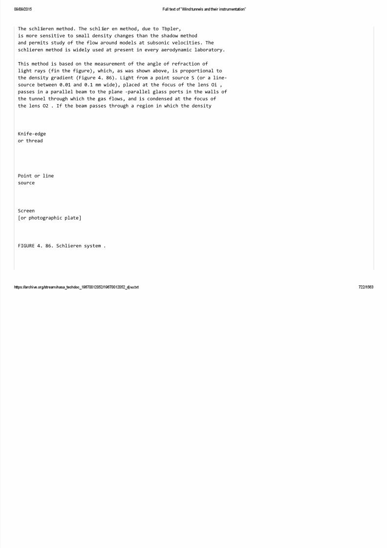
The schl eren method. The schl er en method, due to Tbpler,

is more sensitive to small density changes than the shadow method

and permits study of the flow around models at subsonic velocities. The

schlieren method is widely used at present in every aerodynamic laboratory.

This method is based on the measurement of the angle of refraction of

light rays (fin the figure), which, as was shown above, is proportional to

the density gradient (Figure 4. 86). Light from a point source S (or a line‐

source between 0.01 and 0.1 mm wide), placed at the focus of the lens Oi ,

passes in a parallel beam to the plane ‐parallel glass ports in the walls of

the tunnel through which the gas flows, and is condensed at the focus of

the lens O2 . If the beam passes through a region in which the density

Knife‐edge

or thread

Point or line

source

Screen

[or photographic plate]

FIGURE 4. 86. Schlieren system .

 

varies in the flow direction it is refracted through an angle f and crosses

the focal plane of the lens O2 at a distance B from the optical axis (point A/),

where 8=/‐f , / being the focal length of the lens O2 ■

A thin thread (of about 0.1 mm diameter), passing parallel to the line

source through point N , will cast a shadow on the ground‐glass screen

of a camera, focused on the center line of the tunnel. This shadow indicates

the regions in which the density variations cause the beam to be refracted

through an angle ■( .

Micrometer adjustment, parallel to itself of the shadow thread [or

knife edge] to another position 8| in the focal plane, will cause it to stop all

rays refracted by an angle 71, and so on. Each shaded area (stripe) on the

screen will correspond to a region in which a definite density gradient

exists.

Knowing the value of 5 for each position of the thread we can integrate

the expression

5r^w;r„^» 0.00235 df

to obtain p(.«;), which is approximately

p{x) = p{Xo) + ‐Qj^^jj‐fh(x)dx.

243

 

Thus , knowing the density at a certain point xo , we can determine p at

every point by a single integration.

Instead of a single thread it is possible to use a grid, consisting of

many threads, so that an instantaneous photographic record is obtained

of the fam.ily shadow stripes corresponding to the different density

gradients.

If a knife edge is placed in the focal plane instead of the thread, it will

stop all rays deflected by am.ounts larger than the distance of the knife

edge from the optical axis. The screen of the camera will be shaded for

all regions in which the density gradient exceeds the corresponding value

(Figure 4. 87), and the qualitative flow pattern (compression and

condensation shocks, flow separation, etc.) will appear on the schlieren

photograph.

Wind tunnel

FIGURE 4.87. [Modified] schlieren instrument (according to D. D.Maksutov) ,

Getting sharp (high ‐definition) images by the schlieren method requires

not only great experimental skill and careful adjustment of the instrument,

but also the use of very good telephotographic lenses of the type used in

astronomy. The preparation of such lenses, or of the large parabolic

mirrors sometimes used instead, is very difficult so that it is difficult

 

o cons ruc goo sc eren ns rumen s w e ame ers arger an

200mm. D. D. Maksutov suggested an improved optical design, providing,

at comparative ease, an instrument of high quality and large field of view.

In this system (Figure 4. 87) the light beam from a line source is reflected

from a spherical mirror (1), and passes as a parallel beam first through a

meniscus lens (2), then through the glass port of the wind tunnel and across

the inhomogeneous stream. After emerging from the second port, the light

passes through the second meniscus lens (3), and is reflected by a second

spherical mirror (4) first onto a flat diagonal mirror (5) and then through

the diaphragm (6) (situated at the focus of the second spherical mirror),

onto a screen (7) or onto the eyepiece of a magnifying glass (8). The

preparation of spherical mirrors and meniscus lenses is relatively sinriple,

and by assembling them so as to compensate for their mutual aberration,

high‐quality optical systems can be obtained with considerable field

diameters (up to between 300 and 500mm).

244

Figure 4.88 shows the IAB‐451 [Soviet Union] schlieren instrument,

designed according to Maksutov's principle. The instrument has two main

parts: a collimator I, designed to project a parallel light beam of 230 mm

diameter through the field investigated, and an observation tube n, designed

for visual observation and photography of the schlieren picture.

FIGURE 4. 88. IAB‐451 type schlieren instrument .

 

Meniscus lenses (2) and mirrors (3) are fixed in holders in both

collimator and observation tube. The tubes (1) are mounted on brackets

on opposite sides of the test section of the wind tunnel so that the optical

axes of the mirrors and lenses coincide.

The collimator is fitted with a light source (4), condenser lens (5),

and slit carriage (6), ao that the collimator slit can slide along (for

adjustment at the focus of the optical system) and be rotated about the

collimator axis. The sharpest definition is obtained when the slit is

perpendicular to the direction of the largest density gradient. The slot

is fornned by parallel knife edges with micrometer adjustment of their

separation, so that the slot width can be read off with an accuracy of

0.01mm.

245

The observation tube is fitted with a carriage (7) for the knife edge and

for either interchangeable lenses (8), or a camera adaptor (9). The

carriage (7) serves for focusing the knife edge and for rotating it about

an axis parallel to the slot. In addition, the carriage has a micrometer

slide for adjusting the knife edge in a plane perpendicular to the axis, for

the purpose of stopping the rays from the lens. The position of the knife

edge is indicated on the scale to an accuracy of 0.01 mm..

A drawback of schlieren instruments with large fields of view is that they

extend over a considerable distance outside the wind‐tunnel perpendicular

to its axis. In the design of modern schlieren instruments with 500‐mm.

field diameters the collimator and observation tube are shortened by up

 

o . m y repea e y en ng e op ca ax s w e a o sp er ca

mirrors and inclined lenses.

The interferometric method. The interferometric method

of flow investigation is based on the difference in the velocity of light in

media of different densities. The phenomenon of interference of light

can be understood by considering a light beam as a train of waves. When‐

ever two light beams intersect, they reinforce each other at points where

the wave peaks of one train coincide with those of the other, but cancel

each other at points where the peaks of one train coincide with the

troughs of the other. If two coherent light beams (i. e., beams from two

sources which oscillate in phase or at constant phase difference) converge

at a point on a screen after traveling by different paths, their relative

phase will be determined by the difference between their optical path

lengths. Depending on this difference, they will reinforce or weaken one

another. [Two coherent parallel line sources] will thus project onto a

screen a sequence of dark and light fringes. If both light beams have

passed through a medium of the same density, the interference fringes

will be parallel to each other. If the density of the medium is different over

part of the path of one beam, the light‐propagation velocity (which depends on

density) in this beam will change, and the interference pattern will be

disturbed. Density gradients in the medium will also distort the fringes.

The magnitude of the displacement and change of shape of the fringes

provide a measure of the density changes within the field of view. The

optical interferometer can thus be used for quantitative and qualitative

investigations of the density and for determining the flow pattern around

a model.

The Mach‐Zehnder interferometer is used for aerodynamic research.

The schematic diagram of this instrument is shown in Figure 4. 89. An

image of the light source (1) is focused on the slot (2) of the collimator (l),

situated at the focus of the lens (3). The parallel light beam. from, the

lens (3) falls on the interferometer (II), of which the principal components

are the two half‐silvered plates (4) and (5) and the two mirrors (6) and (7).

 

e p a e v es e g n o wo eams o an o . e eam a, passes

through the glasses (10) and (11) on either side of the test section of the

wind tunnel, and is reflected by the mirror (6) and the half‐silvered

plate (5) onto observation tube (III). The beam aj is reflected by mirror

(7) through the half‐silvered plate (5) onto the observation tube. In this

way plate (4) divides the beam from the collimator (I) into two parts,

which are reunited by plate (5) and focused by lens (8) onto the plane of the

photographic plate or the screen.

246

Depending on the transit time from the common light source to the

camera or screen, the waves in beams ci and 02 will arrive either in

phase or with a finite phase difference. The superimposed beams

produce an interference pattern on the screen, which can be observed

visually or can be photographed.

'Saa^

FIGURE 4. 89. The Mach‐Zehnder interferometer. 1 —collimator with light source;

II —interferometer mirror system; III —observation tube; IV —compensator.

The velocity of light in air increases with decreasing density, so that

 

the trans t t me along a g ven a r path w ll decrease w th decreas ng

density. The interference pattern will be affected by changes in density

along the paths of the beams a, and oj and in particular, by changes in

density in the test section of the wind tunnel, through which beam a, has

passed.

The interferometer can be arranged to obtain, fringes of either infinite

or finite* width. These two methods yield different interference patterns.

For infinite‐width fringes, the plates and mirrors of the interferometer

are installed parallel to each other at an angle of 45° to the flow direction.

When both beams a, and 02 pass through media of the same density, their

optical paths will be equal; they will arrive in phase on the screen, and

the screen will be uinformly illuminated. When the density of the medium

changes uniformly in the test section, the transit time of beam a, will

differ from that of beam oj , so that the light waves in the two beams (which

are coherent since they originate in the same light source) will arrive out

of phase at the screen. A gradual change in density throughout the test

section will cause a corresponding gradual change in the brightness of

the screen, which will be maximum for phase differences corresponding to

1, 2, 3, etc., wavelengths and minimum for phase differences corresponding

to i‐, ii.,2y, 3^. etc. , wavelengths. When the wind tunnel is first

started up the density changes around the model will produce a complicated

interference pattern on the screen, each line being a contour of equal

density. The distance between adjacent lines corresponds to one wave length,

or, as will be shown below, to a change in air density of

4.68 X10‐* kg‐ sec^/m* for a test‐section width of SOOmm. Setting up the

• [Also called fringe‐displacement method.]

 

 

interferometer for fringes of infinite width does not give high accuracy,

since the number of interference fringes is small, and this method is

used only for qualitative analysis.

To obtain data from a large number of points in the field the plate (5)

of the interferometer is rotated so that light beams a, and oj emerge from

it at a small angle a to each other. With undisturbed flow in the test

section, the different path lengths of the beams give rise to an interference

pattern consisting of alternately dark and light straight fringes, whose width

(the distance between the centers of adjacent dark and light regions) is

B = ‐; their direction is perpendicular to the plane containing the axes of the

beams oj , aj • The width and direction of the fringes can be changed by

adjusting the mirrors of the interferometer. When the density of the

air in the test section changes gradually and uniformly, the whole system

of straight interference fringes becomes displaced parallel to itself. A

density change causing a phase shift equivalent to one wavelength X (for

the green spectrum line generally used, I can be taken as 5.5X10~*mm),

will cause the pattern to move by one fringe width. If different rays of

the beam ci cross the test section of the wind tunnel in regions of

different density, (i. e., of different index of refraction n), there will be

a corresponding shift of parts of the interference pattern and deformation

of the fringes. We can measure these shifts, and calculate the difference

of the indices of refraction An — n2 — ni in the corresponding sections of the

tunnel to determine the density changes Ap = p2 — pi in these sections,

assuming that the density along each light path across the test section is

constant, i. e., that the flow is two‐dimensional.

In order to calculate Ap for two‐dimensional air flow we can use the

 

above relat onsh p between the ndex of refract on and the dens ty.

Differentiating, we obtain

af/i = 0.00235 fifp.

The magnitude of the shift of an interference line at a given point in the

xypXaxie, which is perpendicular to the optical axis, is determined by two

photographs, one under static conditions, and the other with full flow in

the test section. This shift is expressed by the number N(x,y) which is

equal to the ratio of the interference ‐fringe shift at the point (x, y) to the

width of this fringe. Knowing N(x,y) we can calculate the corresponding

difference in transit time with and without flow

'2 — f 1 ‐f '

where subscript 1 denotes static conditions and subscript 2, full flow in the

test section, and f is the frequency of light, which is a constant for a

given color and depends on the filter used.

The difference between the transit times of the beams can be expressed

in terms of the change in the speed of light in the test section

‐<, = /( '

i f 2 {x, y) f 1 (AT, y)

)■

 

248

where I is the path length of the beam in the test section. Equating the

last two expressions, we obtain

f \ "2 (x, y) v, (x, y) ] ■

By definition the index of refraction is the ratio of the velocity of light in

vacuo tjyac 'to its velocity v in the given medium:

so that

‐‐7^«vac='l«2(‐<. V) — n^{x, y)l = Mre(A:, y);

since the length of a light wave in vacuo is

then

 

and

1 "vac

vac — f •

N(x, y)X^^^=IAn{x, y) = /• 0.00235 Ap (x, y),

i^P^x, y)— 0,00235; •

If the density pi at zero flow in the tunnel is known, the density of the

flowing medium at a given point can be found from

P2{x, y) = p, + ip(;c, y).

If a monochromatic light source with a green filter is used in the

interferometer, we can take Xvac= 5,5X10"''. In a wind tunnel with a test‐

section width of 500mm, the density change corresponding to a pattern

shift of one fringe width is

'^P= o.*l55^ = '*‐68 ■ '0'* kg‐ secVm*.

The displacement or distortion of the interference fringes can be

measured to an accuracy of 0.1 or 0.2 fringe widths, which correspond to

4p«5‐10"''tol0"' kg‐secVm*.

 

The processing of interferograms in density determinations is shown

schematically in Figure 4. 90. The interference fringes corresponding

to zero flow are indicated by broken lines; those obtained during tunnel

operation, by full lines. We denote by A/1 and AS the changes in

[horizontal] distance from an arbitrary point M at the edge of the field to

points A and B. In the figure, AA is 0.7 of a fringe width and ABis 0.9

of a fringe width. Taking the fringe width as as 4.68X10"*‐ kg‐sec^/m.*,

we obtain the absolute values of the density differences:

ap^ = P^ — P^ = 0.7‐4.68‐ 10' = 3.38‐10~'' kg‐ sec2/m4,

Apg = Pa — P^ = 0.9‐4.68‐ 10^ = 4.21 • 10"" kg‐ sec^ /m* .

249

Illllll

By this method we can measure the difference in densities at points situated

on a vertical line in the field of view. To measure the difference in

densities in the horizontal direction the fringes are obtained horizontally.

The relative error of measuring

the density by the interferometer

increases with Mach number, because

of the decrease in absolute density.

It is simpler to determine the shift

of the fringes if they are first aligned

 

perpend cularly to the chord of the

model or to the wall. Thus, for

instance. Figure 4. 91 shows the

interferogram of flow past a flat plate

with a laminar boundary layer for which

M = 2.04. In this case the density

gradient is normal to the direction of

the fringes at zero flow and each fringe

on the photograph is a line of [constant]

density difference (with density as the

abscissa).

Knowing the density distribution,

we can find the pressure distribution,

for instance, on the surface of a wing.

In this respect the advantage of the interference m.ethod over the mano‐

metric method is that it provides pressure data for a larger number of

points and does not require the preparation of a complicated model with

many orifices.

Pressure can be determined as follows: at any point on the wall of the

test section, a measured pressure p, will correspond to a density p,.

These are related to the flow parameters at any other point by the

expression

FIGURE 4.90. Quantitative interpretation

of interferograms .

P (x. y) ^ fr

 

Po Po

0,00235/p„

or, since po = /)o/g/?7"o.

Po Pa

where

b _ Jvac?^

0.00235/ '

If the flow is isentropic up to the point where the pressure is known,

then p,lpo = (pr/po)", whence

p (X, y)

Po \PJ Po ^ "

 

if the flow is also isentropic up to the point (a;, y) where the pressure is to

be determined, then

p (x, y)

Po

={(tr+*i7^(''>')

1680

250

Thus, in order to determine the pressure at any point (a:, y), it is necessary

to measure the stagnation temperature To, the total pressure po, the

pressure p,, and the relative fringe displacement A^(a:, j/). The pressures

determined in this way are in good agreement with the results of mano‐

metric measurements.

FIGURE 4. 91. Interferogram of a laminar boundary layer on a flat plate ( M = 2.04; Re = 200,000).

 

For accurate quantitative analyses with an interferometer the light

source must be as perfectly monochromatic as possible. The mercury

lamps mostly used for this purpose are fitted with interference filters

which isolate the green mercury line (X= 5. 46X10"* mm). Since clear

interferance pictures demand very short exposures, spark‐light sources

having durations of a few microseconds are also used.

In some modern instruments the interferometer is combined with

a schlieren apparatus, using a separate observation tube mounted

coaxially with the collimator.

The error in measuring the distortion or shift of the fringes of the

interference pattern is about 0.2 fringe width in visual observation and

0.1 fringe width when using photographs. This accuracy is achieved

by the use of a wedge compensator (IV) (Figure 4. 89) inserted into

one branch of the interferometer. The compensator consists of a

hermetically sealed air chamber, one wall of which is formed by a

plane ‐parallel glass plate (12), and the other by a pair of wedge‐shaped

glass plates (13) and (14). Plate (14) can slide over plate (13), thus

forming a plane‐parallel plate, whose thickness can be adjusted to

compensate for the effect of the beam Qi having to pass through the glass

windows of the wind tunnel. The magnitude of the adjustment also indicates

the effects on light‐transit time of changes of air density in the wind tunnel.

The displacement is measured by a micrometer. The compensating air

chamber serves to compensate for changes in the initial density of the air

in the wind tunnel. By changing the pressure inside the chamber, we can

change its equivalent optical thickness.

The interferometric method provides more accurate quantitative results,

than the schlieren method. The principal difficulties in both methods are

due to the fact that all inhomogeneities encountered along the light path in

the wind tunnel are superimposed.

 

In two‐d mens onal flow, where the dens ty s constant along any l ght

path, quantitative measurements present no difficulty to an experienced

251

worker. It is much more difficult to determ.ine the density changes,

when the axis of flow symmetry is perpendicular to the direction of the

light beam.s. Quantitative optical investigations are therefore largely

restricted to two‐dim.ensional problems.

When comparing the use, in qualitative studies, of the interferometer,

shadowgraph, and schlieren instrument, the following should be noted.

The shift of the interference fringes is proportional to the changes in

density of the flowing medium, whereas the results obtained by schlieren

and shadow methods depend to a first approximation respectively on the

first and second derivatives of the density with respect to distance.

a

',ji ' 1 » ■ b

FIGURE 4. 92. Interference (a) and shadow photographs (b)

of flow around airfoil ( M = 0. 95; o = 6° ) .

 

Interference photographs therefore show clearly changes in density for

which other naethods are not sufficiently sensitive. Thus, for instance.

Figure 4. 92 shows interference and shadow photographs for a flow around an

airfoil at M = 0.95. The outer zones of expansion of the gas at the leading

edge, and the density change behind the compression shock and along the

lower surface of the wing can be clearly seen on the interference

photograph. On the other hand, the interferometer is less sensitive to

small sudden changes in density, which are more readily seen on the

shadow picture. This insensitivity to small but sudden changes is useful

because flaws in the windows, or dust on them, reduce the clarity of the

schlieren photographs.

252

Bibliography

1. Loitsy anskii, L. G. Mekhanika zhidkosti i gaza (Mechanics of

Liquids and Gases). — GTTI, Moskva. 1957.

2. Shaw, R. Influence of Hole Dimensions on Static Pressure Measure‐

ments.— J. Fluid Mech., Vol.7, pt.4.1960.

3. Dean, R.C. Aerodynamic Measurements. — Mass. Inst, of

Technology. 1953. ,

 

4. Petunin,A.N. Priemniki dlya izmereniya davleniya i skorosti v

gazovykh potokakh (Probes for Measuring Pressure and Velocity

in Gas Flows). — TsAGI. Collection of articles "Promyshlennaya

Aerodinamiko" Issue No. 19. Oborongiz. 1960,

5. Holder, D.W. Experiments with Static Tubes in Supersonic Air‐

stream. — ARC Rep. Mem., No. 27827 19537‐ "

6. Fizicheskie izmereniya v gazovoi dinamike i pri gorenii (Physical

Measurement in Gas Dynamics and Combustion). — Moskva IL.

1957.

7. Wint e r nit z , F, A. I. Simple Shielded Total Pressure Probes. —

Aircraft Engng., Vol.30, No. 356. 1958.

8. Markowski, S.J. and E. M. Moffat . Instrumentation for

Development of Aircraft Powerplant Components Involving Fluid

Flow. — SAE Quarterly Trans., Vol. 2, No. 1 . 1948.

9. Young, A.D. and J.N. Maas . The Behavior of a Pitot‐Tube in a

Transverse Total ‐ Pressure Gradient. — ARC Rep. and Mem.,

No. 1770. 1937.

10. Barry, F.W. Determination of Mach Number from Pressure

Measurements.— Trans. ASME, Vol.78, No. 3. 1956.

 

. a ov, . . snovy rae ro og un amen a s o e ro ogy . —

Moskva. 1949. ‐

12. Ower,E. The Measurement of Air Streams [Russian Translation]. —

Moskva ‐Leningrad. 1935.

13. Bryer , D.W. Pressure Probes Selected for Three ‐Dimensional

Flow Measurements. — ARC Rep. and Mem., No. 3037. 1958.

14. Fusfeld, K.D. A Probe for Measurements of Flow Inclination

in a Supersonic Air Stream. — J. Aero. Sci., Vol. 18, No. 5. 1951 .

15. Lee, J. C. andJ. E. Ash. A Three ‐Dimensional Spherical Pitot

Probe.— Trans. ASME, Vol.78, No. 5. 1956.

16. Keast,F,H. High Speed Cascade Testing Technique. — Trans.

ASME, Vol.74, No. 5. 1952.

17. Morris, D.E. Calibration of the Flow in the Working Section of the

3 ft X 3 ft Tunnel NAE. — ARC C. P., No. 261. 1956.

18. Raney , D.J. Flow Direction Measurements in Supersonic Wind

Tunnels. — ARC C. P., No. 262. 1956.

19. Gukhmati, A. A. and others. Eksperimental'noe issledovanie

 

pro o no o e aemo ermopary pr ec en gaza s o s o

skorost'ya (Experimental Study of High ‐ Speed Hot Gas Flowing

Lengthwise around a Thermocouple). — Sbornik Trudy TsKTI,

No. 21. 1951.

20. Hottel,H.C. and A. Kalitins ky . Temperature Measurements in

High ‐Velocity Air Streams. ^ J. Appl. Mechanics, Vol.12,

No. 1.1945.

253

21. Malmquist,L. Temperature Measurements in High ‐Velocity Gas

Streams. — Kungl. Tekniska Hogskolans Handlinger. Trans, of the

Royal Inst, of Techn. Stockholm, Sweden, No. 15. 1948.

22. Martinov.A.K. Eksperimental'naya Aerodinamika (Experimental

Aerodynamics). — Oborongiz. 1958.

23. Wood, R.D. A Heated Hypersonic Stagnation Temperature Probe.—

J. of the Aero ‐Space Sci., Vol.27, No. 7. 1960.

24. Monaghan, R. J. The Use of Pitot ‐ Tubes in the Measurements of

Laminar Boundary Layers in Supersonic Flow. — ARC Rep. and

Mem., No. 3056. 1957.

 

. res on, . e erm na on o ur u en ur ace r c on w e

Aid of Pitot Tubes. [Russian Translation] In: Sbornik Perevodov

i obzorov inostrannoi literatury "Mekhanika", No. 6. 1955.

26. Ko ns t ant i no V , N. I. and G. L. D r agny sh . K voprosu ob

izmerenii poverkhnostnogo treniya (The Problem of Measuring

Skin Friction). — Trudy Leningradskogo Politekhnicheskogo

Instituta, No. 176. 1955.

27. Preston, J. H. Visualisation of Boundary Layer Flow. — ARC Rep.

and Mem., No. 2267. 1946.

28. C arter , A.D.S. Some Fluid Dynamic Research Techniques. — The

Institution of Mechanical Engineers Proceedings, Vol. 163

(W.E.P. No. 60). 1950.

254

Chapter V

INSTRUMENTS AND APPARATUS FOR

PRESSURE MEASUREMENT

The pressure measurement is the most important measurement in the

experimental study of the motion of a liquid or a gas. It is sufficient to

note that measuring the pressure is the simplest way to find the magnitude

 

an rec on o e ow ve oc y; y measur ng e s r u on o e

pressures on the surface of a model or in the wake behind it, we can

determine the aerodynamic forces and moments which act on the model

and its separate parts.

The methods of measuring the pressure in a moving liquid or gas are

the subjects of much theoretical and experimental research. Instruments

for measuring pressures are continuously being improved. However,

despite the large number of available designs for measuring instruments,

the researcher sometinnes needs a special instrument which will satisfy

in the best way possible the requirements of certain problems, since very

often standard equipment cannot be used for this purpose.

The pressure of a liquid or gas is determined by the force acting

normally on unit surface. In aerodynamic calculations, the unit of

pressure very often used is that of the technical m‐ kg‐s system, (meter,

kilogram force, sec) which is equal to 1 kg/m^. A pressure of 1 kg per cm^

is called one technical atmosphere or simply one atmosphere. Units of

pressure ordinarily used are the mm of water column (mm H2O) and the

mm of mercury colum.n (mm Hg), i. e., the pressure exerted on its base

by a 1 mm‐high column of the given liquid. The height of the column

corresponds to the normal gravitational acceleration (980.665 cm/sec^)

and to different temperatures (4°C for water and 0°C for mercury). When

measuring pressures by U‐tube manometers, liquids other than water or

mercury are ordinarily used, but the heights of the columns of these

liquids are referred to the heights of the corresponding column of water

or mercury.

The use as unit of measurement of 1 kg/m^ is very convenient in

experimental aerodynamics. The pressure of Ikg/m^ corresponds to

a 1 mm‐high water column. This simplifies calculations according to

the data provided by U‐tube manometers. When measuring pressures

the researcher has to take into account the absolute pressure p, the

gage pressure pg, and the pressure difference Ap . The absolute pressure

 

s e pressure re erre o per ec vacuum. e gage pressure s e

difference between the absolute pressure and the atmospheric (barometric)

pressure B

255

A negative gage pressure is called rarefaction. The pressure difference

is the difference between any two absolute pressures pi and pi

In most cases a manometer is an instrument which measures the gage

pressure. An instrument for naeasuring the pressure difference is usually

called a differential manom.eter. This term is to a certain degree arbitrary,

since the gage pressure also represents the difference between the pressure,

which is of interest to the researcher, and the atmospheric pressure.

In many aerodynamic experiments the most important magnitudes

measured are the pressure differences from which the flow velocity, the

mass flow, and the coefficients of pressure are determined. In other

experiments the absolute pressures are most important. Thus, for

instance, absolute pressure enters in many formulas of gas dynamics.

Most often the absolute pressure is deterniined as the algebraic sum of

the readings of a barometer and of a manometer showing the gage pressure.

A barometer is an instrument which measures the atmospheric pressure

referred to perfect vacuum, and is an essential part of the equipment of

an aerodynamic laboratory.

In addition to manometers which measure pressure differences,

aerodynamic laboratories also use manometers which measure directly

the absolute pressure. The use of "absolute" manometers of special

design for aerodynamic research prevents additional errors due to the

 

arome ers, us re uc ng e me nee e or ca cu a ons.

The main characteristics of manometers are pressure range, accuracy,

sensitivity, linearity, and speed of response.

The range of pressures which can be measured in aerodynamic tests

extends from almost perfect vacuum (for instance in wind tunnels for free

molecular flow) up to several hundreds of atmospheres in supersonic

installations. In shock and pulse tunnels, steady and nonsteady pressures

attaining 3000 to 5000 atm have to be measured. For any given wind tunnel

the pressure range is narrower, but still cannot always be covered by a

single type of manometer.

The accuracy of a manometer can be improved by increasing its

sensitivity. However, an increase in sensitivity is usually concomitant

with a smaller pressure range, since the smaller the permissible relative

error, the more complicated, expensive, and difficult to operate becomes

the m.anometer. The pressure range can be reduced, for instance, by

choosing a comparison pressure close to the measured pressure.

Excessive sensitivity is undesirable in manometers, since a sensitive

manometer, reacting to small disturbances causes an increase in the time

needed for, and sometimes a reduced accuracy of, the measurements.

Maximum accuracy is required in measuring static and total pressures

in wind tunnels for continuous and intermittent operation, since the velocity,

the Mach number of the flow, and all aerodynamic coefficients are determined

from these magnitudes. U‐tube manometers are used for these

measurements, providing measuring accuracies from 0.02 to 0.1% of the

maximum measured value.

256

 

The accuracy requirements are lower for multiple m.anometers by

which the pressure distributions on surfaces are determined, since with

a large number of experim.ental points, the pressure distribution curve

can be drawn sufficiently accurately even if it does not pass through all

points. It is difficult to provide a high measuring accuracy in each

separate tube of a multiple manometer because the absolute pressure

at different points of the body can differ considerably (at hypersonic

velocities by several orders of magnitude).

Linearity is also related to accuracy, because, when the instrument

scale is nonlinear, we have to use approximate functional relationships

in order to simplify the calculations. Therefore, we always try to ensure

proportionality between the measured pressure and the readings of the

manometer, even if this leads to more complicated instruments.

The instruments used for naeasuring pressures in aerodynamic research

can be divided into the following groups :

1) liquid ‐colunrin manometers,

2) pressure gages with elastic sensing elements,

3) pressure transducers,

4) manometers for measuring low absolute pressures.

The operating principle of manometers of the last group is based on

the change of several physical properties of rarified gases when their

pressure varies. A description of these manometers, used for measuring

pressures below 1 mm Hg in special wind tunnels, can be found in the

literature on vacuum techniques /!/.

 

§ 1 9. LIQUID‐ COLUMN MANOMETERS

According to their operating principle, liquid‐column manonaeters can

be divided into two groups : manometers for direct reading, and

manometers of the null type. Manometers for direct reading are used for

measuring the difference in height between the two levels of a liquid in

communicating vessels. Each height is determined in relation to the

stationary instrument frame. In manometers of the null type the franne

is displaced, this displacement being measured after the displacement of

the liquid in relation to the frame is reduced to zero.

Manometric liquids

The medium used in liquid ‐column manometers is most often alcohol,

water, or mercury; the properties of these and other manometric fluids,

which are complicated organic compounds /2/, are shown in Table 9.

The main requirements for manometric fluids are: high chemical

stability, low viscosity, low capillary constant, low coefficient of thermal

expansion, low volatility, low tendency to be contaminated, and low tendency

to absorb moisture from the air. All these requirements are aimed at

increasing the measuring accuracy. Thus, a high chemical stability and

low volatility are important for maintaining a constant specific

257

 

grav ty of the manometr c flu d, on wh ch the manometr c constant depends.

A high viscosity causes an increased transmission lag of the instrument.

Properties of manometric fluids at t‐20°C

Fluid

Methyl alcohol

CH3OH

Ethyl alcohol

CjHjOH

Distilled water

Tetrabromo‐

ethane

02113814

Carbon tetra‐

chloride

CCI4

Ethylene bro‐

mide

Mercury

 

Specific

gravity

g/cm'

Boiling

point

°C at a

pressure

of 760

mm Hg

Surface

tension

dyn/cm

Ethyl bromide

Toluene

0.792

64.7

 

0.789

78.4

0.999

100

(l.Oat

4'C)

3.42

189.5

1 594

76.8

 

2.18

L32

13.55

356,9

(13.59

at O'C)

1.43

38.4

0.866

110.8

 

22.6

22.0

72.8

76.8

26.8

38

465

28,4

TABLE 9

Viscosity

centipoise

 

0.69

1.9

1.000

Coefficient of

volumetric ex‐

pansion X 10

Remarks

Physiological

effects

0.97

1.55

110

15.0

 

18.0

Optimum fluid.

When water is

added, the

specific gravity

increases.

Reacts strongly

with metals

Conodes rubber

Reacts strongly

with rubber

Reacts strongly

with aluminum

copper, and sol‐

dering alloys:

weakly with

iron and steel

the meniscus

should be co‐

 

vere w an

oil film.

Narcotic. Strong

poison

Narcotic. Poison

Narcotic. Poison

Very toxic vapors

Narcotic. Poison

Thernaal expansion of the liquid, causing changes in its specific gravity,

also causes changes in the zero reading and the instrument constant.

Capillarity affects the level of the fluid in the tube, which depends on the

surface tension of the liquid and on its wetting properties. For wetting

liquids the meniscus inside the tube is concave upward and the liquid in

the tube rises under the action of capillary forces above the level of the

liquid in a wide vessel (Figure 5. la). For nonwetting liquids the meniscus

is convex upward and the level of the liquid in the tube is lower than in a

 

w de vessel F gure 5. lb .

The rise and fall of a liquid (the capillary depression) is

A/! =

4o cos (

(5.1)

258

where ‐j is the specific gravity of the liquid, d is the internal diameter

of the tube, 9 is the wetting angle. For a given fluid the coefficient of

surface tension o varies inversely with temperature. Tentatively, we can

write for water: ^h =

30

 

 

for alcohol: AA =

for mercury: AA= — ‐

When measuring low pressures, an important parameter of the liquid

is its vapor pressure, since at a pressure equal to the vapor pressure of

the liquid at a given temperature, the liquid evaporates.

‐^rf U—

b^‐(

1

■C:

 

,

‐

‐l^h

},‐„,„j,„„i,::n,,,,,,irrrri

a ^

<)

■c: ^

V

'

 

FIGURE 5.1. Capiliary change in level of liquid in a tube,

a — wemng liquid: b — nonwetting liquid.

When the internal dianaeter of the manometrlc tube is constant along its

length, the capillary change in level of the liquid can be ignored, since it

will be equal for both tube legs. In noncalibrated tubes the capillary

depression may vary along the height of the tube. In addition, the capillary

depression depends on the state of the internal tube surface and on the

purity of the liquid. For these reasons low values of the capillary

depression should be aimed at. This is achieved by using tubes having

large internal diameters (8 to 12 mm) and by choosing a liquid having a

low surface tension. Alcohol is used in manometers having tubes of snaall

diameter (2 to 5 mm). It should be remembered, however, that alcohol

has a higher coefficient of thermal expansion than water or mercury, so

that alcohol manometers require accurate temperature verification.

Impurities in mercury greatly influence the value of its surface tension, so tha

that mercury has to be cleaned frequently. Dirt on the tube walls not

only prevents accurate reading, but also increases random changes in

shape of the meniscus and in the capillary forces when the mercury rises

or falls in the tube. Contamination of the mercury can be reduced by a

thin film of oil or alcohol on its surface.

U‐tube manometers

The U‐tube manometer consists of two communicating vertical glass

 

u es egs gure . . e pressure erence o e measure s

related to the level difference h in the tubes (legs) of the manometer by the

equation

P\—Pi = ‐\h* ,

(5.2)

More exactly from p, _ p^ = y/i (1 — yi/v) . where hf^ is the specific gravity of the liquid in the left ■

hand leg. The value of Yi/Y 's usually neglected.

259

where t is the specific gravity of the manometric liquid.

This equation shows that the range of the measured pressure differences can

be altered by changing the specific gravity of the liquid and theheight of the tube.

FIGURE S.2. A U‐

tube manomeier.

 

a‐^p^t

FIGURE 5.3. U‐tube mano‐

meter with totaling device.

1 — lead screws; 2 — optical

sighting devices; 3— differential

gear; 4 — counter; 5 — handle

for turning screws.

The sensitivity dh/d{pi — ps), varies inversely with the specific gravity

of the liquid. The maximum practical tube height is about 3 m (i. e., the

height of the laboratory room); hence, the range of pressures which can be

measured by mercury manometers is limited to about 4atmi. The same

height for tubes filled with alcohol corresponds to a pressure range of

about 0.24 atm. It may happen that mercury manometers are not sensitive

enough, while alcohol or water manometers cannot provide the required

measuring range. In such cases recourse is had to heavy liquids, such as

tetrabromoethane, carbon tetrachloride, and Thoulet solution (a solution of

mercuric iodide in potassium iodide).

When the manometer is filled with water, the reading of the height

differences in m.m gives the numerical value of the pressure difference in

kg/m^.

Since the diameters of the glass tubes are in general not uniform along

their length, the level difference h must be calculated from the change in

 

e g o e co umns o qu n o egs. n excep on o s ru e s

260

a specially calibrated tube. Usually U‐tube manometers are equipped with

sliding scales; before the experiment the zero graduation is adjusted to the

level of the liquid in both legs.

If the height of the column of liquid is read by the naked eye, the absolute

error in height may be about 0.5 mm. Since two readings are required

for determining the height difference, the error may attain 1 to 2 mm.

When higher accuracy is required, the manometers are equipped with optical

reading devices.

Figure 5.3 shows a U‐tube manometer with a device permitting the

difference in height in both legs to be determined without intermediate

calculations. For this purpose the sighting devices (2) are located at the

level of the meniscuses with the aid of lead screws (1) which are connected

to the differential gear (3). The latter is connected to counter (4), on which

the height difference ft is read off.

If the above precautions are taken to reduce the influence of surface

tension in the U‐tube manometer, it can be used as a primary instrument

which requires no calibration by another [reference] instrument. The only

correction necessary is for the influence of temperature. The true

difference in the levels of the liquid, expressed through the specific gravity

of the liquid at temperature to, is

 

w ere , an correspon o e empera ure

is made, or

(5.3)

at which the measurement

A,r =''/

l‐HPC^‐'o) '

where g is the coefficient of volumetric expansion of the liquid.

(5.4)

Pi‐Pe'/A^yifi

FIGURE 5. 4. Effect of liquid, present in the

connecting tube on the manometer readings.

 

  . . e ‐ ype mano‐

meter.

For accurate pressure m.easurements, it is sometimes necessary to

make a correction for temperature distortions of the scale. In order to

reduce the reading to the temperature to at which the scale was etched,

we use the equation

Ao = Att b + <^it‐io)l

(5.5)

261

where a is the coefficient of linear expansion of the material from which

the scale is naade.

In order to prevent loss of liquid from the manometer when the pressure

varies abruptly, traps in the form of wells or widenings in the upper parts

of the tubes are provided. When liquid is present in the inclined connecting

tube (due to overflowing or condensation), the actual pressure difference

will exceed by fzhi the readings of the manometer (Figure 5.4). In order to

prevent the collection of liquid in the tube bends they are best arranged in

the m.anner shown in Figure 5. 4 by broken lines.

 

Well ‐type manometers

The drawback of U‐tube naanometers is the necessity to read the

indications of two tubes. This is avoided in the well‐type manometer.

(Figure 5. 5) which is a U‐tube manometer one of whose legs has a

larger cross section than the other. The higher pressure acts on the

leg having the larger cross section (well). Under the action of the

pressure difference, the liquid rises in the glass tube to a height hi, and

falls in the well by an amount fe . The height of the columin which balances

the pressure difference is

A = Ai ‐j‐ ^2‐

Since the volume of the liquid displaced from the well, whose cross ‐

sectional area is F2, is equal to the volume of the liquid which enters the

measuring tube, whose cross ‐sectional area is Fi, the measured pressure

difference is

/'.‐/'2 = M(i‐F‐^)‐ (5.6)

The ratio F,/F2 allows for the change in level of the manometric fluid

in the well. To avoid additional calculations, the cross ‐sectional area

ratio should be very small (< 1/500); it is either ignored, or special

scales are made.

Figure 5. 6. shows schematically an electrical device for automatically

measuring the level of the liquid in the tube of a well ‐type mercury

 

manome er . cons s s o a servo sys em, w ose sens ng e emen

is a photo‐electric cell mounted on a movable carriage together with a

lamp throwing a light beam, through the liquid onto the photo‐electric cell.

When the meniscus moves in relation to the light beam, the Wheatstone

bridge into one arm of which the photoelectric cell in inserted (semiconductor

resistance), becomes unbalanced, and an amplified imbalance signal is fed

to a servomotor which with the aid of a naicrometer screw returns the

carriage to a position fixed in relation to the meniscus. The displacement

of the carriage is m.easured by a counter connected to the micrometer

screw. The range of the measured pressures is only limited by the length

of the micrometer screw, while the accuracy of the device depends on the

262

accuracy of the alignment of the carriage with the meniscus

(0.15 to 0.25 mm). Such a servo device simplifies the task of the

FIGURE 5.6. Device for automatically

measuring the height of a mercury column. 1 —

tube filled with mercury: 2 ~ micrometric

screw : 3 — guide column: 4 — carriage; 5 —

photoelectric cell; 6 — Wheatstone bridge;

7— a.c. amplifier; 8 —bridge ‐supply transformer;

9 — lamp‐supply transformer: 10 — rectifier;

11 — lamp; 12 — servomotor; 13— counter.

experimenter, freeing him from, the work of visually aligning the sighting

 

dev ce w th the men scus n the tube.

Liquid ‐column micronianom.eters

These are sensitive manometers designed for indicating pressure

differences from a few up to 500 mm W.G. at errors between a few

tenths and a few thousandths of a millimeter. The lower limit of the

pressure range mentioned is found, for instance, in boundary‐layer

velocity investigations. Thus, the velocity head of air at atm.ospherIc

pressure, flowing at 10 and Im/sec, is 6 and 0.06 mm W.G. respectively;

for measuring these velocities with an accuracy of 1%, the micromanometer

error must not exceed 0.12 and 0.0012 mm W.G. respectively.

The sensitivity of liquid‐column manometers is raised by increasing the

displacement per unit pressure difference, of the meniscus in relation to

263

the stationary tube walls and by increasing the accuracy in measuring this

displacement with the aid of optical devices.

Two ‐fluid micromanometers. If the legs of a U‐tube manometer

are enlarged at the top to form two wide vessels and are filled with two

immiscible liquids whose specific gravities are ti and T2 (Figure 5.7), we

can observe the displacement of the interface separating the two liquids.

 

 

Interface

1

Ml

‐1'

un

At

r,

FIGURE 5.7. Two‐ fluid

 

m cromanometer.

FIGURE 5.8. Increase of meniscus dis‐

placement in a narrow connecting tube.

We then have

A ‐ ‐"2 = ‐^ [(T2 ‐ 71) + ^ (T2‐f Ti)]^

(5.7)

where h is the displacement of the interface under the action of a pressure

difference pi — pi = ls.p, and F| and F^ are respectively the cross ‐sectional areas

of the tube and the well, which for simplicity are assumed to be the same

for both legs. When F^IF^ is very small, the displacement is approximately

T2 — Ti

(5.8)

 

The immiscible liquids may be, for instance, ethyl alcohol and kerosene.

For naeasuring small pressure differences in rarefied gases it is

suggested /14/ to use liquid organosilicon polymers whose vapor pressures

vary between 10"* and 10"^ mm Hg (the vapor pressures of mercury and

water are 1.2X10"^ and 17.5mm Hg respectively). The value of 72 — 11

varies between 0,07 and 0,2g/cm , The use of liquids whose specific

gravities differ less reduces the response of the naanometer and causes

large temperature errors.

Bubble micromanometers. A widely used method of increasing

the displacement of the meniscus is illustrated in Figure 5.8. The

displacement / of an air bubble or an oil drop in the tube connecting the

wide vessels (1) and (2), can be found for a two‐fluid manometer frora (5. 7),

if we put ‐[I = f2 = f . In this case the sensitivity of the instrument is

h

2 F, If

(5.9)

264

 

The designs of many sensitive micromanometers intended for measuring

very small pressure differences are based on this principle, e, g,, the

Chattock gage, which is widely used in Great Britain and the U. S. A. /5/.

,p.

^ A^

^i>'

II

/». ^^^

h, h

r

2

 

‐~"‐^^‐_r‐

^

FIGURE 6.9. Inclined micromanometer.

A peculiarity of this micromanometer is that small pressure differences

are measured by returning the bubble to its initial position in relation

to the instrument frame, which is tilted with the aid of a micro‐

metric screw connected to the scale which is graduated in units of pressure.

D i r e c t ‐ r e a d i ng in cl in e d ‐ tub e micromanometers. A

simple method of increasing the displacement of a meniscus in relation to

the tube walls consists in inclining the tube at an acute angle to the horizontal

(Figure 5. 9). This is one of the most widely used instruments for

measuring flow velocities in low‐speed tunnels. The relationship between

the displacement of the liquid along the tube axis and the measured pressure

difference is

/>.— i'2 = T'(sina + ‐^j.

(5.10)

 

The sensitivity of the micromanometer can thus be increased by

reducing the specific gravity of the liquid, the angle of inclination of the

tube a, or the area ratio FilF^. Alcohol is ordinarily used in inclined‐

tube micromanometers. In order to reduce capillarity effects, calibrated

tubes having internal diam.eters of 1.5 to 3 mm are used.

Soviet wind tunnels are largely equipped with TsAGI micromanometers

(Figure 5. 10). This instrument has a cylindrical well rigidly connected to

a glass tube enclosed in a metal casing. The tube is provided with a

manometric scale graduated to 200 mm. By rotating the well about its

horizontal axis, the tube can be inclined so thatsina= 0.125; 0.25; 0.5;

and 1.0. The ratio between the cross ‐sectional areas of the tube and the

well is 1/700.

Inclined ‐tube micromanometers are equipped with levels which permit

adjustments of the horizontal position of the stand. These micromano‐

meters have to be calibrated, since slight bends in the tubes or small

changes in capillary depression, due to small variations of the internal

tube diameter, may cause considerable errors.

The errors due to capillarity in inclined‐tube manometers are the

same as in vertical manometers. There exists therefore a minimum

265

{■■■■III ■Hill

 

angle a, below which no increase in sensitivity is obtained because of

the capillarity error. In practice a = 6°.

FIGURE 5.10. TsAGI mioromanometer. 1— clamp‐

ing device ; 2 — glass tube; 3 — spigot: 4— rotating

well; 5 — casing.

FIGURE 5.11 Null‐type liquid‐column micromanometer. a — with movable

inclined tube; b — with movable well; 1 — inclined tube; 2 — micrometric screw;

3 — scale for reading number of screw turns; 4 — scale for reading angle of rotation

of screw; 5 — well; 6, 7 — flexible tubes; 8 — sighting device.

Inclined null rQicromanometers. The capillarity error can be

reduced considerably by using manometers in which the level of the liquid

is held in a constant null position in relation to the walls of the capillary

tube.

In the null mioromanometer shown in Figure 5. 11a, the inclined

capillary tube is movable and has a null line on it. The position in which

the m.eniscus is aligned with this line is called the zero position of the

 

266

instrument. When the pressure difference changes, the inclined tube is

moved until the meniscus is again aligned with the null. This is done

with the aid of a micrometric screw. The meniscus is observed with the

aid of a sighting device which moves together with the inclined tube.

The second type of null micromanometer (5. lib) differs from the former

in that the inclined tube is stationary; in order to return the meniscus to the

null position the well has to be moved. Because of this, the meniscus can

be observed with the aid of a stationary microscope, while the eye of the

observer is always at constant level. Such a device permits the measured

pressure difference to be increased up to 500 or 600 mm W.G. The reading

accuracy of the column of liquid depends mainly on the manufacturing

accuracy of the micrometric screw, and attains 0.03 to 0.05 mm.

In experinnents requiring accurate measurements of pressure, attention

must be paid to reducing the transmission lag of manometers. For instance,

when determining the velocity profile in a boundary layer by a tube having an

internal diameter of 0.2 to 0.4 mm, the transmission lag of the manometer

amounts to tens of seconds and sometimes to minutes. The errors caused

by the lag are not only due to the fact that readings are made before the

pressure in the tube orifice is in equilibrium with the pressure in the well,

but because during the time required for the complete series of measurements,

the temperature of the surroundings can change (for instance, due to heat

transfer through the walls of the wind tunnel). The volume of liquid in both

legs of a liquid‐column null micromanometer at the instance of reading

remains the same, irrespective of the measured pressure difference. The lag,

due to the flow of liquid from one leg to the other, therefore depends only on

 

e s o e exper men er or on e response o e au oma c ev ce

used) in realigning the meniscus with the null line.

Increasing the sensitivity of a null micromanometer by increasing the

inclination of the capillary tube increases the lag (the volume of displaced

liquid increases for a given pressure difference).

A temperature change of the liquid in a well ‐type micromanometer

causes a change in the zero reading; for this there are two reasons:

1) the change in volume of the liquid due to thermal expansion;

2) the change of the surface tension of the liquid in the capillary tube.

These factors act in opposition, and thus may compensate mutually.

The relationship between the geometrical parameters of the manometer,

necessary for the compensation of temperature changes, is when the well

is made of steel and is filled with alcohol /6/:

T^ = 0.29 cm',

where v is the volume of the liquid‐column micromanometer; d is the

internal diameter of the tube; Ft is the area of the well cross section.

This compensation enables the temperature error of the micromano‐

meter to be reduced to less than 0,01 mm/l°C /7/.

Float ‐type micromanometers. Determining the position of a

meniscus "by accurate measurements requires much effort. In float ‐type

micromanometers, the position of a solid body floating on the surface of

the liquid is determined instead of the position of the meniscus.

 

 

Figure 5.12 shows a float ‐type raicromanonieter ‐which enables

differences up to 200 mm W.G. to be measured. The difference in level of

the liquid between the annular well (2) and the cylinder (1) is measured

with the aid of scale (3) which is attached to a body floating on the surface

of the liquid in the cylinder. The scale can be observed and the difference

in level read off through window (4) and microscope (5). The micrometric

device (6) serves for aligning the sighting line of the microscope with the

null line of the scale.

Bridge —

Recording

Springs

FIGURE 5.12 Float‐type micromanometer with

optical reading. 1 — cylinder ; 2 — annular welt

3 — scale; 4 — window; 5 — microscope; 6 —

aligning device.

 

FIGURE 5.13. Float‐ type micromanometer with

remote indication.

In another float ‐type micromanometer /8/, intended for m.easuring

pressure differences up to 25 mm W. G., the position of the float in relation

to the walls of the vessel is recorded with the aid of an induction‐type

displacement transducer connected to an electronic bridge. The float is

secured to the walls of the vessel with the aid of six 0.075 mm thick wires,

which are tensioned in pairs by 3 flat springs located at angles of 120°

around the axis of the float (Figure 5. 13). This instrument is calibrated

by displacing the liquid with the aid of a piston moved by a micrometric

screw. The accuracy of the instrument depends on the sensitivity of the

transducer and the measuring system, connected to it.

An error of less than 0.5% of the measurement range is difficult to obtain,

but by reducing the m.easurement range to 1 mm W. G., the absolute error

can be reduced to about 0.005 mm.

268

Balance ‐type mi c r omanomet er s. Very high sensitivity and

accuracy can be obtained with micromanometers in which measuring

the height of a column of liquid is replaced by measuring forces with the

aid of balances.

In the instrument shown in Figure 5. 14 the pressures pi and pj act via

 

e as c me a u es on e qu n commun ca ng vesse s moun e on e

arms of a balance. If the right‐hand vessel is at a higher pressure,

some liquid will flow from, it into the left‐hand vessel. Equilibrium is

restored either nnanually or automatically by moving a counterweight. The

sensitivity of this instrument is independent of the specific gravity of the

manometric liquid. For vessels of given height, a change in the liquid is

only reflected in the range of measured pressure differences.

x‐jpy

^

y‐Pz

l^'^^^^

^

/

 

'>/////////.

FIGURE S,14. Compensated manometer. 1 — lever;

2 — servomotor for lead screw; 3 — movable counter‐

weight; 4 — contact system for switching on the servo‐

motor when the lever is not in null position; 5 — com‐

municating vessels; 6 — elastic tubes.

Figure 5. 15 shows a bell‐type manometer for direct readi.‐.g. Pressures

/?, and p2 act on the inside of communicating vessels (bells) (1) and (2),

FIGURE 5.15. Bell‐type manometer. 1 and 2 — bells; 3 — balance lever;

4 — communicating vessels; 5 — UJ.iisparent scale; 6— screen; 7 — mirror;

8 — light source.

269

which are suspended from a balance lever (3). The open ends of the bells

are immersed in the liquid contained in vessels (4). Under the action of the

pressure difference som.e liquid is forced out from one bell into the other, and

the lever tilts by a small angle which is proportional to the pressure

difference and depends on the sensitivity of the balance. This angle can be

 

measure y eren me o s, or ns ance, w e a o an op ca

system which projects an enlarged image of the transparent scale (5) onto

the screen (6).

In compensated bell‐type manometers (Figure 5. 14) the lever is returned

to the null position with the aid of a movable counterweight, whose travel

is proportional to the measured pressure difference.

Damping the pulsations of the columns of

liquid in manometers

The pressures measured in different aerodynamic test installations

are very seldom steady. Usually the pressure fluctuates about a certain

mean value. The amplitude and wave form of these pulsations depend on

the design and type of the installation. The oscillations of the columns of

liquid in manometric tubes, caused by the pressure pulsations,

reduce the measuring accuracy. In order to prevent build‐up of oscillations,

forced damping sometimes becomes necessary.

There exist three ways of damping in manometers: inertial, volumetric,

and resistance damping. Volumetric damping is applied to manometers

in which large changes in volume are required for measuring small

pressure differences, as for instance, in manometers where the cross ‐

sectional areas of the tubes are large. Inertial damping is used when the

liquid has a large mass. The inertia of the mass prevents motion caused

by sudden pressure pulses of short duration. Inertial dam.ping is not always

sufficient for damping oscillations of the level of the liquid. Resistance

damping is caused by resistance ofthesystem, which limits the flow velocity

of the liquid during sudden pressure pulsations. This type of damping is

very effective, and is easily obtained in existing manometers by inserting

a damping resistance. In order that the manometer readings correspond to

a mean value, the resistance must be linear, i. e., proportional to the flow

 

ve oc y o e qu . on near amp ng may occur a ro e s nser e

into the pneumatic or hydraulic line of the instrument. Linear ("viscous")

damping is obtained simply by inserting a capillary tube into the pneumatic

line of the instrument. The tube length is chosen by experiment, taking

into account that an excessive length may cause considerable transmission

lag in the manometer. Another method of resistance damping of the liquid ‐

column oscillations in a m.anomieter is to insert small felt or cotton‐wool

pads into the pneumatic line of the instrument.

§ 20. MECHANICAL MANOMETERS

Manometers with elastic sensing elennents and small moving masses

have a quicker response than liquid‐column manometers. The transmission

270

lag in such manometers is determined mainly by the time required for

the equalization of the pressure in the chamber of the elastic element with

the pressure to be mieasured, whereas in liquid‐column manometers an

additional lag is caused by the displacement of the liquid. Using elastic

elements, and keeping the volume of the pressure chamber small, we can

reduce the dinaensions of the manometer and install it near the place where

the pressure is being measured. When the volume of the chamber and the

length of the connecting tube are reduced, the transmission lag of the

manometer decreases.

Due to their high natural frequency, elastic elements can be used for

measuring not only steady but also fluctuating pressures. Pressures are

 

measure y m.eans o e as c e emen s y e erm n ng e er e

defornaation of an elastic element or the force required to prevent the

deformation (force ‐compensation method).

The deformation of the elastic elem.ents is measured with the aid of

kinenaatic, optical, or electric systems. Kinenaatic pointer ‐type or

recording instruments and optical devices are used mainly in spring‐type

m.anometers, while electric systems are found in pressure transducers.

In comparison with the method of determining the pressure from the

deformation of elastic elements, the force‐compensation method is more

exact since it enables the effects of elastic hysteresis to be reduced. How‐

ever, the force ‐compensation method requires more time. When measuring

rapidly fluctuating pressures, only the first method is therefore used. The

force ‐compensation method is used for measuring steady or slowly varying

pressures when the error must not exceed 0.1 to 0.5% of the upper limit

of the measured value.

Types of elastic elements

The following three types of elastic sensing elements are most widely

used: Bourdon tubes, bellows, and diaphragms (flat or corrugated).

The operating principle of a Bourdon‐tube manometer is well‐known.

Under the action of the pressure, a tube of oval or elliptic cross section,

bent in a circular arc (Figure 5. 16a), tends to straighten itself. The

displacement of the tube end is measured with the aid of a kinematic device.

 

I I

FIGURE 5.16 Elastic elements for measuring pressures, a — Bourdon tube;

b — spiral tube; c — tlat diaphragm; d — corrugated diaphragm and set of

aneroid boxes; e — bellows.

271

The action of a spiral tube (Figure 5. 16b) is based on the same principle.

Flat diaphragms (Figure 5. 16c), which have higher natural frequencies

than Bourdon tubes, can be used for measuring high‐frequency pressure

pulsations. Flat diaphragms can be installed flush with the surface of a

body. The pressure to be m.easured acts directly on the diaphragm, hence

there is no transmission lag, due to the resistance of the connecting tubes

and the volume of air in the system.

The sensitivity of a flat diaphragm, which can be considered as a plate

fixed along a circular contour, can be defined as the ratio of the deformation

8 at the center of the diaphragm to the pressure p

._ 6 _ 3(1‐1x2) r'

 

16£ k'

The natural frequency of the diaphragm, which should be 3 to 4 times

higher than the frequency of the pressure pulsations, is

'^^■^[‐wvc^J'

where r and h are respectively the radius and the thickness of the diaphragm,

while E, n, and pare respectively the modulus of elasticity, Poisson's ratio,

and the density of the diaphragm material. Thus, the sensitivity and the

natural frequency are related by the equation

The sensitivity of a diaphragm, is inversely proportional to the square

of its natural frequency and to its thickness. The sensitivity of a diaphragm

can therefore be increased by lowering its natural frequency. The

sensitivity of a diaphragm ‐type manoraeter depends not only on the value of

k but also on the method used for measuring the deformation of the

diaphragm.

The range of pressure differences which can be measured with a single

diaphragm depends on its thickness and diameter, and varies from hundredths

of a mm Hg to thousands of atmospheres. Since the absolute deformations

of a flat diaphragm are very small, they are measured by optical or

electrical methods. Mechanical naethods change the natural frequency of

the system because of the masses connected to the instrument. Electrical

methods are simpler and do not lead to large dimensions, as do optical

 

methods. For a g ven sens t v ty of the d aphragm, the sens t v ty of the

manometric system can be increased only by anaplifying the output signal

which corresponds to a given deflection of the diaphragm.

Corrugated diaphragms permit considerably larger deflections than

flat diaphragms. For even larger deflections, corrugated diaphragms

are m.ade in the form of boxes which can be assembled into sets

(Figure 5. 16d).

Bellows are most widely used in the design of manometers employed

for m.easuring steady pressures in wind tunnels. A bellows (Figure 16e)

is a cylindrical thin‐walled tube with uniform folds. The presence of a

large number of folds makes possible large deformations of the moving

bottom of the bellows under the action of pressure differences.

272

The gage pressure acts inside the bellows or the vessel which surrounds

it. The movable bottom of the bellows, which is connected with the

measuring mechanisna of the manometer, can be considered as a piston

moving without friction in a cylinder under the action of the pressure

forces, and loaded by a spring which, in this case, is formed by the folds

of the bellows.

The bellows is nnade of brass, phosphorus‐bronze, beryllium‐bronze,

or stainless steel. Brass bellows are most widely used, but their hysteresis

is high (up to 3% of the full travel). The hysteresis of bellows made of

beryllium ‐bronze or phosphorus‐bronze is lower.

The characteristics of a bellows as a mieasuring element depend on two

 

ac ors: e r g y c, an e e ec ve area . e r g y s e

ratio of the force acting on the moving bottom of the bellows to its travel 5.

The effective area of the bellows is the ratio of the force N to the gage

pressure p required to restore the bottom of the bellows to its original

position:

The maximum permissible travel of the bottom of the bellows is about

5 to 10% of the bellows length, if residual deformations are to be avoided.

Proportionality between the travel and the force acting on the bottom is

best maintained if the bellows is subjected to compression.

The ratio of the length to the outside diameter of the bellows should be

less than unity. When the bellows is longer, there is a danger of longitudinal

instability caused by bending and transverse deformation of the bellows. In

order to prevent this the movable bottom of the bellows is usually connected

to a guiding device which ensures axial travel of the bottom.

Spring‐type manometers

Sta.ndard manometers with spring‐type sensing elements in the form of

Bourdon tubes have errors of 1 to 3% of the scale range, which are

inacceptible for aerodynamic measurements. For certain types of multi‐

point measurements (for instance, in testing engines or compressors), B our don ‐

tube reference manometers made by the Soviet industry are suitable ; they are

from high‐quality material and have low hysteresis. The scale of a

reference manometer has 300 one‐degree graduations on a convex scale.

Reference manometers are available for measuring negative pressures

down to 760mm Hg vacuum, and positive pressures up to 1.5, 5, 10,

25, and 50 kg/cm ^ or more. According to the existing specifications for

mianometers, the permissible measurement errors are as follows: for

vacuum meters and manometers for pressures up to 2 kg /cm," ±0.35% of

the scale limit; for manometers for pressures above 2kg/ cm^, ±0.2%

 

of the scale l m t.

The accuracy of spring‐type manometers can be increased by reducing

or eliminating friction in the transmission mechanism. When friction is

eliminated, the accuracy of the manometer is mainly determined by the

hysteresis of the elastic element.

273

An example of a frictionless spring‐type manometer is the manometer

in which the deflection of the Bourdon tube is measured with the aid of an

accurate micrometric mechanism or a dial indicator (5) (Figure 5.17). The

micrometric mechanism is isolated from the tube (1), to which the flexible

contact plate (2) is soldered. A second flexible plate (3) is soldered to the

micrometer screw. Electric contact between the plates is sensed by a so‐

called "magic eye" electronic tube normally used in radio receivers. The

wiring diagram is shown in Figure 5.17. To measure the pressure, contact

between the screw and tube is first broken. Plate (3) is then slowly brought

back into contact with plate (2); this is sensed by the "m.agic eye. " Such a

device permits the error to be reduced to 1/2 or 1/3 of the error of a

reference manometer with pointer, but this is acconnpanied by an increase

in time required.

‐1

 

Mi..

FIGURE 5.17. Spring‐type manometer with contacts.

1 — Bourdon tube; 2 and 3— contact plates; 4 —

micrometric device: 5 — dial indicator.

FIGURE 6.18. Pendulum‐t>pe manometer. 1 —

pendulum; 2 — lamp; 3 — lens; 4 — transparent

scale; 5 — screen.

When using bellows made of tompac or semitompac for spring‐type

manometers, the influence of hysteresis of the bellows is reduced by an

additional spring of high‐quality steel or beryllium‐bronze. In this case

the elastic force of the bellows is small in comparison with the elastic

force of the spring which has a low hysteresis, and therefore, the error

due to hysteresis of the bellows decreases proportionally with the ratio

of the rigidities of bellows and spring. The reduction in sensitivity of

the elastic element, caused by the additional spring, is compensated for

by the higher transmission ratio to the pointer.

Bellows manometers have measurement errors of the order of 1%.

The error can be reduced to 0.2 to 0.5% when the bellows are of

beryllium‐bronze or phosphorous‐bronze. Bellows manometers can be

used to measure pressures between perfect vacuum and 10 to 20 atm.

 

In the bellows ‐type pendulum manometer, shown schematically in

Figure 5.18, the elastic force of the additional spring is replaced by

the restoring moment of the pendulum (1), which eliminates the influence

of the hysteresis of the bellows. For angles of pendulum inclination

below a = 6°, the relationship between the pressure and the angle is linear.

274

being expressed as follows with an accuracy better than 3%:

Here, G is the weight of the pendulum counterpoise, p is the gage pressure

acting inside the bellows, a is the distance between the pendulum support

and the center line of the bellows. By altering the weight of the counter‐

poise or the length / of the pendulum, we can vary the range of the

measured pressures. The influence of hysteresis of the bellows can be

almost eliminated by selecting the ratio of the static moment of the

pendulum to the rigidity of the bellows so that Gl'^ca''. Accurate

measurement of the angular displacement of the pendulum is ensured

by an optical system consisting of lamp (2) which projects, with the aid

of lens (3), a large image of scale (4) on screen (5).

Force‐compensation manometers

Manometers in which the deflections of elastic elements are measured

have errors caused by hysteresis and the influence of temperature on the

rigidity of those elements. Such errors can almost completely be avoided if

the pressure force acting on the elastic element is equilibrated by a force

 

w c re urns e e as c e emen o s n a pos on.

The equilibrating force can be caused by mechanical or electric

mechanisms. The former include devices which use counterweights or

springs; the latter include devices based on the interaction of magnetic or

electrostatic fields. Compensation is effected automatically in certain

instruments.

Oneof thebest designs of force‐compensation manometers for wind

tunnels is a combination of bellows or sets of aneroid boxes with automatic

beam‐type balances. Such a bellows ‐type manometer is shown in

Figure 5. 19. Bellows (1) and (2) are connected to balance lever (3) on either

FIGURE 5 19. Automatic force‐competisation beam‐type mano‐

meter 1 and 2 — bellows; 3 — balance lever; 4 — transducer

cont'rollng the servomotor, 5 — servomotor; 6 — lead screw; 7 —

counterweight: 8 — counter.

side of the knife edge. The pressures p, and p^, whose difference has to

be measured, act inside the bellows. When the pressure difference changes.

275

the equilibrium is disturbed and transducer (4) reacts to the displacement

of the beam end by switching on servomotor (5), which turns lead screw

(6) to move counterweight (7), creating a moment which restores the lever

 

o s n a pos on. e rave o e coun erwe g s measure y‐

counter (8). The wiring diagrams of automatic servomotor controls for

lever ‐type balances are described in Chapter VI.

Let the beam be in the initial position when px—p^ . When the pressures

are varied, the equation of equilibrium becomes

<^/'2^efj‐«i/'i^efi=0'^'

where a, and Oa are the arms of the pressure forces acting respectively

on bellows 1 and 2; fef, and Fef^are the effective areas of these bellows.

G is the weight of the counterweight; x is the displacement of the counter‐

weight from its initial equilibrium position (for pi = pj ).

In order that the displacment of the counterweight be proportional to

the pressure difference p, — p^, it is necessary that

In this case the equilibrium conditions for the lever is

t^p=Pi — Pi = An,

where n is the number of turns of the lead screw, corresponding to the

displacement x , recorded by counter (8) (the screw has a pitch /)■

^— aF ■

If the bellows (1) is acted upon by atmospheric pressure (p, = b) , then

P2 — B = An, and the instrument will naeasure gage pressure. If bellows

(1) is evacuated (pi = 0) and soldered, the manometer will show the

absolute pressure p2 = An. In the latter case we naust take into account

that when bellows (2) is connected to atmosphere, a force BFgi, will act

on bellows (1), which naust be balanced with the aid of an additional

counterweight.

 

n prac ce s cu o o a n a pa r o e ows w c ave equa

effective areas. In accurate bellows ‐type manometers, one of the arms oi

or Qi is therefore adjustable.

Figure 5. 20 shows a set, consisting of two automatic lever‐type balance

elements, which serve to measure pressure differences and the static gage

pressure in the Moskva University wind tunnel. The lever‐type

balances are installed one on top of the other, while the bellows are located

on a bracket fixed to the instrument base, and linked to the levers by rods

and cross beams. The static pressure acts on the bellows at the extrem.e

right, which is linked by a rod to the lever of the upper balance.

The accuracy of such manometers depends largely on the design of the

connections between the bellows and the crossbeams, which must ensure

perfectly axial displacement of the bellows. For this purpose elastic

hinged sleeves are provided (shown in the lower part of the picture).

276

FIGURE 5.20. Sel of lever‐type balances for measuring

Ap and p,

which prevent displacement of the rods in the direction perpendicular to

the center line of the bellows. In order that the forces acting on the knife

edges at the contact points between the rods and the levers be of constant

sign, irrespective of the pressures in the bellows, the cross beams are

provided with counterweights, so that the total weight acting on each knife

edge exceeds the produrt of maximum negative pressure and effective

area of the bellows.

 

FIGURE 5 21 RAE automatic self‐ balancing capsule iranometer 1 — servomotor;

2 — lead screw; 3 — elastic cross‐shaped hinge; 4 — counterweight; 5 — induc‐

tive transducer; 6 — set of evacuated aneroid boxes; 7 — connecting element; 8 —

set of aneroid boxes under pressure.

277

Figure 5. 21 shows the connections between the aneroid boxes and the

levers in the automatic self ‐balancing capsule manometer of the RAE

laboratory /9/. The lever is mounted on a cross ‐shaped hinge and linked

to the aneroid boxes, which are rigidly interconnected, by a flexible strip.

The drawback of this design is the requirement that the aneroid boxes have

exactly equal effective areas.

The accuracy of such a manometer is mainly determined by two factors :

the insensitivity of transducers to displacements and the rigidity of the

bellows. If the insensitivity range of the transducer corresponds to a bellows

displacement ±5, the random error of pressure measurement, due to the

unbalanced residual electric force, will not exceed

%=±7;

 

e

For most industrial bellows the ratio of the rigidity c to the effective area

Fgf varies between 0.1 and Ikg/cm^. In order that the value of o^ should

not exceed 1 mm Hg, the value of s must be less than from 0.013 to 0.13 mm.

The contact and inductive transducers

at the end of the lever, whose dis‐

placement is many times larger than

the deflection of the bellows, permit

measurenaent of 5 with an error of

10"^ to 10"^ mm. With a good ‐quality

lead screw, which moves the counter‐

weight, and when pressure differences

up to 3000 to 4000mm Hg are being

measured, the errors of compensation‐

type manometers may be a few

hundredths of a percent of the maximum

measured value. With bellows of low

rigidity and large effective area, such

m.anometers perm.it measurements of

absolute pressures between 10 and

20mjmi Hg with an error not exceeding

0.1 mm Hg. In order to reduce the

influence of rigidity of the bellows, the

sensitivity of the lever system of the

manometer is increased with the aid

of compensating devices described in

Chapter VI.

Since remote indication of the angle

of turn of the lead screw is possible,

 

ever ‐ ype e ows manome ers are

widely used for measuring total

pressure, static pressure, and

the pressure drop in the test section of subsonic and continuously

or intermittently operating supersonic wind tunnels.

Another manometer design in which a bellows is also used as elastic

element and a counterweight as a compensating element is shown in

Figure 5. 22. Pressures, whose difference has to be m.easured, act

inside the hermetically sealed chamber (1) and the bellows (2), which

FIGURE 5.22. Pendulum‐type compensation

manometer, 1 — hermetically sealed chamber;

2 — bellows; 3 — lever; 4 — elastic cross‐shaped

hinge; 5 — counterweight ; 6 — contacts; 7 —

signal lamps; 8 — micrometric screw; 9 and

10 — links for scale linearizing; 11 — hinge.

278

is connected to lever (3) fixed to an elastic hinge (4). A rod with counter‐

weight (5) is fixed to the lever. In order to return to its initial relative position

the lever (3), which is deflected by the action of the difference of pressure

on the movable bottom of the bellows, the charaber is turned about hinge

(11) by an angle a. This is controlled with the aid of contacts (6) and signal

lamps (7) which go out when the initial position is reached. The value of the

angle a is related to the measured pressure difference as follows:

 

(P2—P\) Fsl^ = Q' sin a,

where f^f is the effective area of the bellows, a is the distance from the

point of support of the lever to the center line of the bellows, / is the

distance from the point of support to the center of gravity of the pendulum,

Q is the weight of the pendulum together with the counterweight. It is

assumed that when pj — Pi =0 then a = 0, i.e., the center of gravity of the

pendulum and part of the bellows lies on the vertical through the point of

support.

HGURE 5 23 Elecironugnetic conipeiuaiion‐

lype manometer 1 — bellows; 2 — di?place‐

niem transducer, '1 — coil; 4 — permanent

magnet, ■') — amplifier, b — tiutliammeter

To provide a linear scale, the micrometric screw (8) moves the

chamber with the aid of an intermediate link (9) hinged to chamber (1)

and link (10) of length L. The relationship between the pressure difference

and the travel y of the screw is given by p2 — p, = my , where m = QljF^^aL is

the instrument constant.

Figure 5. 23 shows a manometer with electromagnetic force compensation

/lO/, which can be used for measuring pressures fluctuating at frequencies

of up to lOkc. The pressure acting on bellows (1) displaces the moving

system with fixed coil (3) which is placed in the field of permanent

magnet (4). The displacement transducer (2) sends a signal to amplifier

(5). The output current of the amplifier passes through coil (3), its

intensity and direction being such that the interaction force between the

 

279

II ■ 1 1 1 1 1 1 II ■ I I

11 III I III

■III II la II I I I I 1 1 II

III IBIIIIIIiaBBII I

coil and the magnet balances the pressure force. The pressure is

determined from the current intensity /, indicated by milliammeter (6),

or from the voltage U across an output resistance R. When the voltage

is m.easured, this circuit provides for a sufficiently strong signal, and

the measurements can be automatically recorded. Thus, at a maximum

current intensity /= 30 ma and with a resistance R— 2500 ohm the voltage

U= 75 V. The error of such an electromagnetic manometer is only 0.1%;

for measuring pressure differences from several millimeters to several

hundreds of millimeters Hg, it can compete with liquid‐column

manometers.

 

‐ <!,.. .....,.....»>>A'! \'^\\^

y

FIGURE 5. 24. Capacitive compensation‐type manometer. 1— diaphragm;

2 —metal electrodes: 3 —annular inserts: 4 —ceramic insulators: 5 — nuts.

For measuring very small pressure differences (up to 1 mm Hg) the

manometer shown in Figure 5. 24 can be used. It is a compensation ‐type

manometer in which the force of the pressure acting on the diaphragm is

balanced by an electrostatic force /ll/. The 0.02mm‐thick stainless ‐

steel diaphragm (1) is held between annular inserts (3). Metal electrodes

(2) are rigidly connected to the inserts (3) by means of ceramic insulators

(4). The tension of the diaphragm can be adjusted by nuts (5).

The capacitor formed by the diaphragm and the electrodes is connected

to the arms of a capacitive bridge fed from a 500kc signal generator

according to the circuit shown in Figure 5. 25. The displacement of the

diaphragm, due to the difference in pressures on either side, is compensated

280

 

by an electrostatic force, adjusted with the aid of a calibrated

potentiometer /?, . At a constant supply voltage Vo, the scale of the micro‐

manometer is linear. By varying Ko, we change the sensitivity of the

instrument. The series ‐connected inductances and capacitances i‐iC,, Z.2C2 ,

L3C3 and L^C, are tuned to the signal‐generator frequency. The signal at

the bridge output, caused by the deflection of the diaphragm, is amplified,

and then measured by a microammeter. Observing the latter, the reading

is reduced to zero by means of the calibrated potentiometer. At zero

reading, the diaphragm returns to its initial position, and the position of

the potentiometer R2 gives the pressure difference. The potentiometer R,

serves for the initial balancing of the bridge. In the pressure range from

10"^ to 10"^ mm Hg, the instrument error is only 0.1%. The design of

the manometer permits pressure differences up to one atmosphere; there‐

fore, if we connect one side of the diaphragm to vacuum (obtained, for

instance, with the aid of a diffusion pump) the instrument will indicate

absolute pressures in the above‐mentioned range.

Signal ® 2iC^

 — [Ampli T^

LferJ‐S^ ,

y di, Meter (null

ohmp^^^^h indicator)

 

generator

ZWpf

ZiOpf?^^:

Wohn

/MQ

V.‐u

ffi^#r#^

JTL

 

jm \^

‐(^0*0)

J^ Capacitive

; Micro‐

manometer

FIGURE 5 25 Wiring diagram of a capacitive

compensation‐t>pe manometer

§ 21. ELECTRICAL PRESSURE TRANSDUCERS

AND MICROMANOMETERS

Pressure transducers are instruments which convert the deformation

of an elastic pressure‐sensitive element into an electric signal.

In connection with experimental research on high‐speed aircraft,

methods for measuring variable pressures have been developed in

recent years. These measurements are necessary when investigating

dynamic loads due to vibrations, and also for studying problems of dynamic

stability of aircraft components. Thus, for instance, when considering wing

 

281

flutter, we sometimes determine transient aerodynamic forces by

investigating the pressure distribution on a vibrating wing. The

measurements are made by special miniature pressure transducers,

(of 5 to 6 mm diameter),, which are placed directly on the surface of the

model or inside its body, close to the orifices. The nature of the

investigated problems does not demand a high measuring accuracy.

Good transducers permit the error in measuring the amplitude of pressure

pulsations to be reduced to between 1 and 2%, but often transducers are

acceptable which permit the pressure to be measured with an accuracy of

from 5 to 10% of the maximum amplitude.

Quite different requirements apply to high‐ sensitivity transducers, used

for measuring steady or slowly‐varying pressures. Such transducers are

used in intermittently‐operated supersonic wind tunnels where measurement

by liquid‐column manometers is not always possible because of high lag.

Such transducers can have comparatively low natural frequencies, but must

have much smaller errors than transducers for measuring dynamic

processes. High sensitivity is usually obtained with transducers of

relatively large dimensions.

If the transducer is connected by a tube to an orifice in the wall, then,

with high‐frequency pulsations the pressure close to the elastic pressure‐

sensing element of the transducer may differ in phase and amplitude from

the pressure on the wall. To reduce dynamic distortions, the lowest

5

 

1^2^3‐*^‐^5‐^6

FIGURE 5,26, Schematic layout for recording

pressure pulsations. 1 — carrier ‐frequency

oscillator; 2— measuring bridge; 3— amplifier;

4— rectifier; 5— filter; 6— oscillograph; 7—

transducer.

resonance frequency of the pressure‐measuring system must be higher than

the highest frequency of the measured pressure pulsations. The lowest

acoustic‐resonance frequency of a closed pipe of length L is

a

where a is the velocity of sound. The amplitude distortions caused by

the elastic pressure‐sensing element can be reduced by increasing its

natural frequency. In order that the error should not exceed 6 to 7%,

this natural frequency must be 4 to 5 times higher than that of the measured

pressure pulsations. Best results are obtained by sensing elements

shaped like flat diaphragms.

Pressure transducers whose operating principle is based on measuring

changes in inductive, capacitive, or ohmic resistances, caused by the

deformation of an elastic element, are mainly used in aerodynamic

experiments. Bridge systems are most widely used for these measurements.

 

1680

282

Although there exist many different schemes for measuring varying

pressures, the above‐mentioned types of transducers are usually

employed as shown schematically in Figure 5. 26. The measuring bridge,

one, two, or all four arms of which are formed by transducers, is fed from,

a carrier ‐frequency oscillator. The amplifier, connected to the measuring

diagonal of the bridge, amplifies the imbalance signals caused by the

changes in transducer resistance due to the pressure variations. The

amplified signals are transmitted through a phase ‐sensitive detector and

a filter, which discriminates the carrier frequency, and are then

measured by a galvanonaeter or loop oscillograph. The carrier frequency

must be 6 to 10 tim.es higher than the frequency of the investigated process.

Inductive transducers

The design principle of inductive transducers is based on the changes

in the inductance of a coil, caused by changes in the magnetic permeability of a

circuit consisting of a core, a magnetic circuit, and a ferromagnetic

elastic element. The latter is usually a flat steel diaphragm, which, when

deformed, alters the air gap between it and the core of the coil which is

Tt

 

‐o o‐

_^,

§

s

 — o o‐

 — ‐■‐— " — ■■■■ »■■■■■

jm BBj gg jH[

J

 

FIGURE 5. 27. Circuits for inductive pressure transducers.

connected to an a. c. circuit. The reactance of the coil depends on the air

gap, and when the coil is inserted into a measuring bridge ‐circuit, the

change in air gap, due to the variation of the pressure acting on the

diaphragm, causes a proportional imbalance signal.

283

Figure 5.27 shows three arrangements for connecting inductive

transducers in a measuring bridge fed from a transformer 7"^ . In

Figure 5.27a, three arms of the bridge are fixed inductors. The fourth arm Lj

is a variable inductor. One of the pressures whose difference is being

measured acts directly on the outer surface of the diaphragm, while

the other pressure acts upon the internal area of the transducer. A

differential circuit (Figure 5. 27b) is ordinarily used for increased

sensitivity. The diaphragm is placed between two inductive coils i, and Li.

FIGURE 5. 28. Miniature inductive

transducer, i — body; 2 — coiis;

3 — coil leads: 4 — diaphragm sol‐

dered to body .

 

FIGURE 5,29 Circuit diagram of an

indiictive transducer with rectifiers. 1 —

supply voltage; 2 — differential inductive

transducer; 3 — rectifiers; 4 — zero ad‐

justment; 5 — oscillograph.

The movement of the diaphragm causes an increase in the inductance of one

coil and a decrease in the inductance of the other coil; the amplitude of the

signal is twice that obtained in the circuit shown in Figure 5. 27a.

The circuit in Figure 5. 27c has an even higher sensitivity, A pivoted

armature connected to the elastic element of the nnanometer changes the

inductance of all four arms of the bridge.

Figure 5. 28 shows a typical miniature inductive transducer for measuring

pulsating pressures. The thickness of the diaphragm can vary from 0.025 mm

(for measuring pressure differences of the order of 25 mm Hg)

to 0.25 m.m for measuring pressure difference of the order of 7atm. When

the am.plitude of pressure pulsations, small in comparison with the

mean pressure, has to be measured, the diaphragm has a hole whose

diameter is between 0.05 and 0.1mm. To reduce temperature effects, the

transducer coil is made of naanganin wire. The accuracy of measuring

the am.plitudes of pressure pulsations with these transducers depend on

the type of equipment used, and naay vary from 2 to 10% of the mtaxim‐um

measured value.

Since the frequencies used in inductive transducers do not exceed a few

kc, the indications are usually recorded by loop oscillographs. When two

or four arms of the bridge have variable inductors, a sufficiently strong

 

s gna can e o a ne w ou an amp er. s s mp es e use o

inductive transducers for simultaneous pressure measurements at several

284

points. A simple and sensitive bridge circuit in which one half of the

bridge is formed by semiconductor rectifiers is shown in Figure 5. 29.

To record low‐frequency pressure pulsations (up to 4 to 5 cycles), balanced

measuring circuits with fast‐acting electronic bridges can be used

(Figure 5.30).

FIGURE S.30. Circuit diagram of a balanced

bridge for measuring liie signal Irom an in‐

ductive transducer. 1 — inductive tranducer ;

2 — sensitivity adjustment: 3 — zero

adjusttnent; 4 — transformer; 5 — servo‐

motor; 6 — amplifier.

An example of an inductive pressure transducer, whose sensitivity is

comparable to that of liquid ‐column manometers, is the NPL inductive

micromanometer /12/ shown in Figure 5.31. This instrument is intended

for remote measurement of pressure differences of up to 100 mm W. G., and

 

FIGURE 5,31. NPL inductive micromanometer. 1 — lever; 2 — elastic hinge; 3 and

4— bellows acted upon by pressures to be measured; 5 and 6— bellows serving for

damping vibrations; 7 — connecting cfiannel ; 8 —soft‐iron plate; 9 — counterweight;

Lj— primary induction coll.

285

consists of four bellows connected to lever (1) which is supported on an

elastic cross ‐shaped hinge (2). Bellows (3) 'and (4) are acted upon by the

pressures whose difference has to be measured; the other two bellows (5)

and (6), interconnected by channel (7), are filled with oil and serve as

dampers. One end of lever (1) carries a soft ‐iron plate (8), balanced by

counterweight (9) on the other end of the lever. When the lever is displaced

due to the pressure difference p,— pjin bellows (3) and (4), the air gap

between plate (8) and the induction coil i, changes. This causes an

imbalance in the inductive bridge (Figure 5. 32). The rectified imbalance

current causes the pointer of galvanometer (6) to be deflected.

Pressure transducer

(Figure 5,31)

^^gb^‐jTjfl Balancing and

counting device

 

{W/i

FIGURE 5.32 Circuit diagram of an inductive

micromanometer. 1 — iron plate; 2 —micro‐

metric screw; 3 — reversible electric motor;

4 ~ reduction gear; 5 — counter; 6 — galvano‐

meter; Li — primary induction coil; Lg — secondary

induction coil.

The bridge is balanced by adjusting the air gap in the secondary induction

coil Z,2 with the aid of iron plate (1) which is moved in the magnetic field of

coil Z,2 by micrometric screw (2). The screw is rotated by a low‐power

electric motor (3) through a reduction gear (4) having a large transmission

ratio. The displacement of plate (1) in relation to coil Li , required to

restore the balance of the bridge, is proportional to the difference between

the pressures in the bellows, and is measured by counter (5) connected

to the reduction gear. Very sm.all pressure differences can be naeasured

directly v/ith the galvanometer by the unbalanced ‐bridge method.

Capacitive transducers

A capacitive transducer for measuring the deflection of an elastic diaphragm

uses a capacitor one of whose plates is the diaphragm itself, the other plate

286

 

being fixed. The capacitor is connected into a suitable electric circuit

which produces a signal which depends on the capacitance.

Maximum sensitivity to pressure changes is ensured in a capacitive

manometer by a very small air gap. However, a linear relationship

between the change in capacitance and the change in pressure requires

the distance between the plates to be large in comparison with the mean

deflection of the diaphragm. Thus, the increased sensitivity of a

capacitive manometer reduces the linearity, and vice versa. In practice,

a compromise has to be accepted. Sometimes, a thick diaphragm is used.

Its deflections are small, but the air gap can be reduced. However, it

should be taken into account that when the air gap is reduced, temperature

effects increase; temperature changes can cause harmful deformations of

the diaphragm.

FIGURE 5,33. Capacitive pressure

transducer. 1 — diaphragm; 2 —

indeformable electrode: 3 — high‐

frequency insulator

Figure 5. 33 shows a small capacitive pressure transducer in which the

diaphragm is integral with the body. The insulation of the fixed plate is

made of ceramic material offering a large impedance to high frequencies.

To remove internal stresses in the transducer diaphragm, which are

liable to increase temperature effects, the diaphragm is heat‐treated

before and after being machined.

 

  ap ragm n egra w e o y as a ower ys eres s an one

clamped at the edges. However, the range of measured pressures is

easier to change in clamped diaphragms. With diaphragms of different

thicknesses and diameters we can make capacitive manometers and

transducers for pressures ranging from fractions of a mm Hg to thousands

of atmospheres. In the lower part of this range, corrugated diaphragms

having thicknesses of up to 0.025 mm and diameters fromi 50 to 100mm

are used; they are made of silver or bronze. When low absolute pressures

have to be measured, one side of the diaphragm is subjected to a pressure

close to perfect vacuum.

In addition to ordinary capacitive transducers, wide use is made of

differential capacitive transducers. Such a transducer consists of two

series‐connected capacitors, with a common plate in the middle serving

as the diaphragm. When the differential transducer is connected to the

287

measuring circuit, the sensitivity is doubled in comparison with an

ordinary transducer; a linear relationship between the deflection of the

diaphragm and the output voltage of the circuit is obtained.

The RAE miniature differential capacitive transducer intended for

investigating wing flutter /13/, is shown in Figure 5.34. The diaphragm

is located between two fixed electrodes, while the air gaps on both sides

of the diaphragm are connected to the upper and lower wing surfaces.

Several tens of these transducers, which permit the force normal to the

wing section to be measured, are fixed to the wing.

 

FIGURE 5.34. Differential capacitive

pressure transducer. 1 — diaphragm ;

2 — electrodes; 3 — electric leads.

When the diaphragm is deflected due to a difference in pressure across

it, the capacitance of the condenser formed by the diaphragm and one of

the fixed electrodes increases, while the capacitance of the condenser

formed by the diaphragm and the other electrode decreases.

FIGURE 5.35. Circuit diagram of a differential capa‐

citive pressure transducer. 1 — transducer; 2 —

carrier‐ frequency amplifier; 3 — demodulator; 4 —

filter; 5 — zero adjustment; 6 — carrier‐ frequency

oscillator.

288

The capacitors are connected to adjacent arms of an a. c. bridge whose

other two arms are formed by mutually coupled induction coils (Figure 5. 35).

The coils are wound in opposite directions; when the bridge is balanced

equal currents pass through them, and the resulting field equals zero. The

output signal of the bridge is taken from a third winding inductively coupled

to the first two. The capacitor C serves for noise suppression. The bridge

 

s e rom a c carr er‐ requency osc a or, w c perm s requenc es

up to about 3000 cycles to be recorded. The output voltage of the bridge,

which is about lOOmV at a maximum pressure difference of 0,3kg/cm^, is

fed via an amplifier to an oscillograph.

B2 Rubber

Polysterene

Mica

FIGURE 5, 36. Differential capacilive manometer. 1— diaphragm:

2 — fixed disc.

The combined errors of these transducers and the measuring circuits

are about ±3% of full scale. The transducers are not sensitive to

accelerations normal to the plane of the diaphragm; this is very important

when measuring pressures acting on a vibrating wing. When the bridge iS

fed at a carrier frequency of 400 kc, it is possible to measure transient

processes (for instance, in shock tubes). At an input‐tube length of

3 mm, the transducers permit pulsation frequencies of up to 15,000 cycles

to be measured; they can be used for turbulence investigations.

A capacitive micromanometer, designed for measuring pressure

differences from zero to 10mm W.G. at low frequencies, is shown in

Figure 5. 36,

A steel diaphragm (1), having a thickness of 0.05 mm and a diameter

 

o mm, s c ampe e ween s ee anges. mm‐ ame er sc s xe

at a distance of 0.01 mm from diaphragm (1). The capacitance of the

condenser is about 80pF, its sensitivity being 0.23 pF per mm W.G.

289

A peculiarity of this manometer is the low temperature dependence of the

capacitance, which at room temperature is about 0.1% per 1°C /14/.

To measure the frequency signals of capacitive transducers, resonance

circuits are used in addition to bridge systenns. A simple resonance

circuit of an electronic amplifier, used in measuring very low steady

pressures, is shown in Figure 5. 37 /15/. The circuit contains only one

electronic tube, which operates as an oscillator. The frequency of

oscillations is determined by the capacitance of the condenser Ci , which

changes when the pressure acting on the diaphragm, varies.

The resonant circuit used for measuring this frequency consists of

inductance Ij and capacitor Cs. The shaft of the latter is connected to an

indicating pointer and to a handle, with the aid of which the capacitor is

tuned into resonance with the second harmonic frequency of the oscillator.

The point of resonance is determined approximately when minimum plate

current, measured by milliammeter Mi, flows through the tube. Final

tuning of the capacitor Cs is carried out using the fine ‐adjustment galvano‐

meter Afj .

250t

 

FIGURE 5.37. Resonance measuring circuit; Ci‐

capacitive manometer; d ‐ 20 pF maximum:

c,i = lOOpF; c, = 15pF maximum; c, ‐ 0.01 uF;

c, = 0.1 uF; c„ c, = O.OliiF ; /?, = l&O K oiim;

Ri, /?, = 85 K ohm; ^, ‐ 60 K ohm, VR, , vr, =

60 K ohm; z.,, i, ‐ 15 turns, ai, ‐ nuliiam‐

mecer for 5 ma; /iij ‐ galvanometer for 540 oiim.

Capacitive manometers of this type are used for measuring pressures

from 0.001 to 0.1 mm Hg. The corrugated diaphragm, made of silver,

copper, or bronze, has a thickness of 0.025 mm and an external diameter

of 76 mm; the diameter of the flat central part is 18 mm. The same

electronic circuit is suitable for other pressure ranges and diaphragm

dimensions.

The drawback of this measurement method is the effect of parasitic

capacitances, mainly in the connecting wires. To reduce errors caused

by parasitic capacitances the transducers are connected to the measuring

circuit by screened cables.

290

strain‐gage transducers

Strain gages, whose operating principle is described in Chapter VI,

 

prov e s mp e n n a ure rans ucers or measur ng var a e pressures

acting on the surface of a model. Both glued wire and foil strain gages are

used for pressure transducers, as are nonglued tension wires.

In small transducers, wire strain‐gages having 2.5 to 5mm bases are

glued directly to diaphragms which are integral with the body or soldered

to it (Figure 5. 38). Such transducers are used by

NACA for installation in airfoils, and are employed

in investigating pressure pulsations ranging from.

0.07 to 1.4kg/cm^ 116/ . Temperature compensation

in transducers of this type whose diameters are

between 6 and 12 mm is effected with the aid of a

second strain gage glued to the body. When the

mean pressure need not be measured, temperature

compensation is not necessary. In ONERA

transducers, intended for this purpose, (Figure 5.39)

the deflection of the corrugated diaphragm is

measured with the aid of wire strain gages glued to

both sides of the diaphragm for temperature

compensation. The diaphragm is located inside a

cylindrical body having a diameter of 10 mm and a

height of 3 mm 1 11 1 . The strain gages, whose

dimensions are 6X2.5 mm and whose resistance is 120 ohm, are inserted

into the arms of a half ‐bridge. At the maximum deflection of the diaphragm,

which corresponds to a pressure difference of 0.15 kg/ cm^, the relative

imbalance of the bridge is 0.5 ‐10"^.

FIGURE 5.38. Strain‐gage

pressure transducer, 1 —

body; 2 — diaphragm; 3 —

 

res s ance s ra n gage.

FIGURE 5,39. Strain‐gage pressure

transducer with corrugated diaphragm.

1 — diaphragm; 2 — body; 3 — strain

gage; 4 — leads.

Glued strain gages with small bases, used in the pressure

transducers described, have low resistances, and consequently, to

limit the current, a low supply voltage is required. At large currents

the heat dissolves the glue. A low supply voltage necessitates a higher

291

signal amplification, Nonglued resistance strain gages are used to obtain

stronger signals. They disperse heat better and therefore permit higher

supply voltages, and hence stronger output signals.

yjK

 

FIGURE 5.40. Pressure transducer with a nonglued strain gage. 1 — cross‐

shaped spring; 2 — rod; 3 — disc; 4 — body; 5 _ diaphragm; 6 — sup‐

port of insulating material; 7 — leads.

In the transducer shown in Figure 5. 40 /18/, the deflection of the

diaphragm is transmitted to an elastic element consisting of two cross ‐

shaped springs (1) interconnected by four rods (2). The spring is fixed

to a disc (3) whose position can be adjusted along the center line of body

(4) which is covered by diaphragm (5). When the diaphragm is deflected,

an axial force acts on the elastic element, bending springs (1) and

causing rods (2), to move outward. The strain gage, which is wound

around rods (2), is inserted into two opposite arms of a Wheatstone bridge.

The other two arnas, which serve for temperature compensation of the

bridge, are formed by a wire wound around the undeformed supports (6)

which are fixed to disc (3). Since all four bridge arms are located in the

sam.e way inside one housing, temperature equilibrium is attained very

quickly. When fitting the springs into body (4), the position of disc (3)

is adjusted in such a way that the strain‐ gage wire is slightly prestressed.

A variable resistance is inserted between adjacent bridge arms in order

to balance the bridge after this adjustnaent. When the supply is 10 V d. c.

the transducers can be connected to sensitive galvanom^eters or oscillo‐

graphs without amplification.

In transducers intended for measuring steady pressures, the wire

strain ‐gages are very often placed on auxiliary elastic elenaents (for

instance, on cantilever beams) connected to the sensing elements

(diaphragms, aneroid boxes, or bellows) on which the pressures act

(Figure 5. 41). A bellows is best, since for equal diam.eters of the elastic

elements and at equal rigidities of the auxiliary elements it permits the

292

 

highest load to be taken up.

are respectively

For bellows and for diaphragms these loads

' + ^

and N^ = \p‐rl

where Cc and Cm are respectively the rigidities of the bellows and the

diaphragm when acted upon by a concentrated load, c^^ is the rigidity

of the beam, r^ is the effective radius of the bellows and r„ is the

radius at which the diaphragm is fixed. When re = r„ Cm is much larger than

Cc at the same pressures, hence Nc>Nk, i.e., considerably higher loads

can be transmitted to the beam by means of a bellows than by means of a

diaphragm.

P!

 

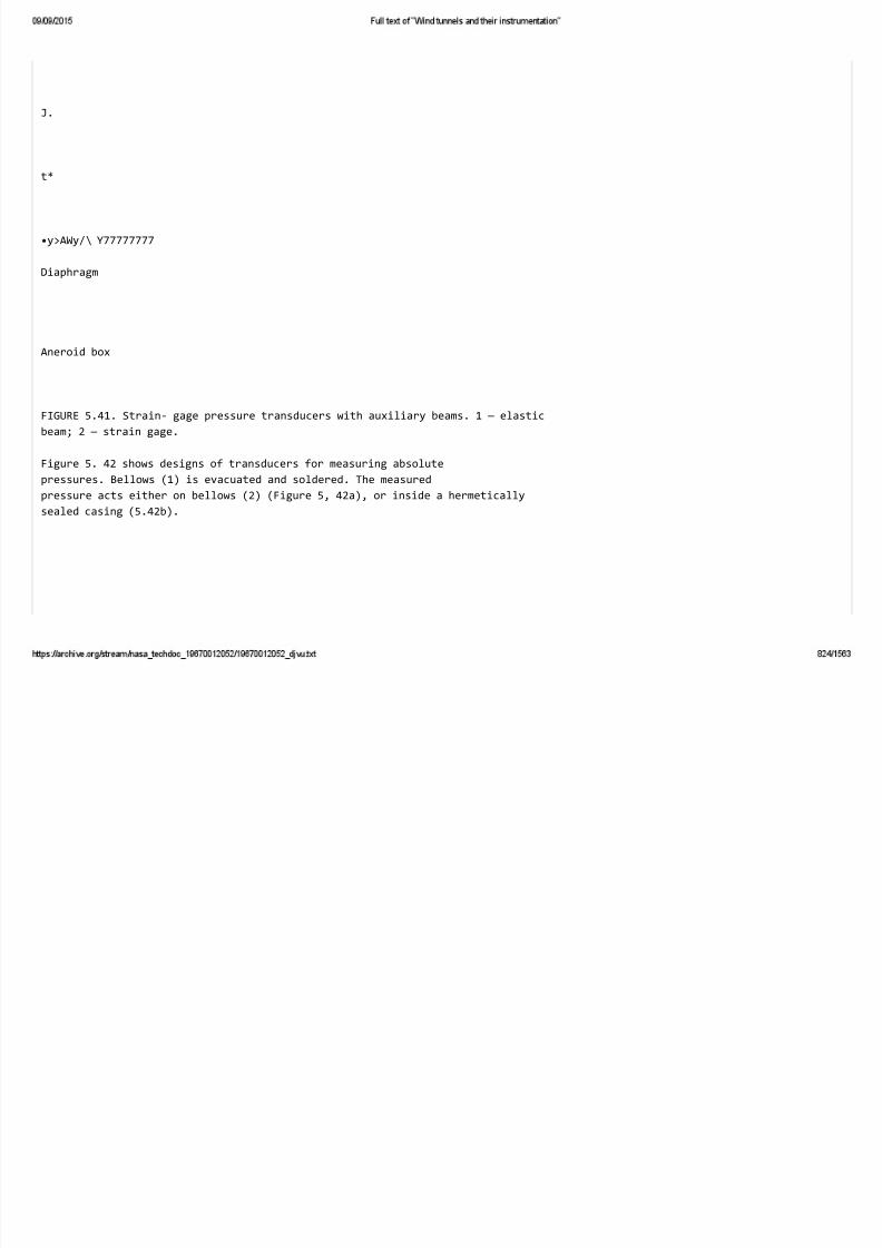
J.

t*

•y>AWy/\ Y77777777

Diaphragm

Aneroid box

FIGURE 5.41. Strain‐ gage pressure transducers with auxiliary beams. 1 — elastic

beam; 2 — strain gage.

Figure 5. 42 shows designs of transducers for measuring absolute

pressures. Bellows (1) is evacuated and soldered. The measured

pressure acts either on bellows (2) (Figure 5, 42a), or inside a hermetically

sealed casing (5.42b).

 

FIGURE 6.42. Transducers for measuring

absolute pressures. 1 and 2— bellows;

3 — elastic element; 4 — hermetically

sealed casing.

293

In addition to diaphragms and bellows, pressure transducers are also

used in which the axial and tangential stresses are determined on the walls

of a tube whose inside is under the pressure to be measured. When metal

tubes are used, such transducers have high natural frequencies, but due

to the difficulties in making thin‐walled tubes they can be used only for high

pressures (tens and hundreds of atmospheres). If rubber or plastic tubes

instead of metal tubes are employed, such transducers can be used for

much lower pressures.

15 MM

FIGURE 5.43. Pressure transducers in a vibrating

wing.

 

n u e‐ ype s ra n‐gage rans ucer or measur ng pressures on

airfoils oscillating at frequencies of up to twenty cycles in a low‐speed wind

tunnel /19/ is shown in Figure 5. 43. The main element of the transducer

is a cylindrical rubber tube to which a wire strain gage forming two arms

of a Wheatstone bridge is glued. The tube itself is glued to a plastic beam,

which has openings for leading in the pressure acting on one of the

measuring points on the wing. The outside wall of the rubber tube is under

the pressure acting on a point on the opposite surface of the wing; the

transducer thus records the difference of the pressures on both surfaces.

The resistance of each bridge arm is 250ohm. The signals of the

transducer, which is suitable for pressure differences up to 3 00 mm

mercury, can be measured without amplifier with the aid of a sensitive

recording galvanometer.

§ 22. EQUIPMENT FOR MEASURING PRESSURE

DISTRIBUTION. MULTIPLE MANOMETERS

The most widely used instrument for measuring pressure distributions

is a liquid‐ column multiple manometer. Such manometers very often

294

I ■■■■■IIIIIH^IH

function according to the principle of well‐type manometers. U‐tube

manometers are used only when the measured pressure differences may

 

ave eren s gns.

^^

^\.jujMt‐W‐'«‐tujt

FIGURE 5.44. Schematic view of a

well‐type multiple manometer.

A well‐type multiple manometer is shown in Figure 5. 44. The well

and the outermost tubes are under the pressure p with which the other

pressures p,‐ are to be compared. The outermost tubes serve for controlling

the level of the liquid in the well.

@^

\n^C^5\\\\V;;^V^^\\n\<^\N^

Plexiglas

Glass tubes

 

FIGURE 5.45. Well‐ type multiple manometer.

A typical well ‐type multiple manometer designed for measuring

pressures corresponding to relatively high columns of liquid (up to 2

or 3 m) is shown in Figure 5. 45. To prevent bending of the glass tubes

they are located in slots milled into Plexiglas shields. Marks, spaced

5 or 10mm, into which black paint is rubbed, are etched on the Plexi‐

glas. Numbers which correspond to the column height in centimeters

are written on both sides of these lines. The use of Plexiglas permits

295

the scale and the tubes to be illuminated from the rear for photographing.

The upper part of the instrument contains a nunaerator, which enables

the number of the experiment, the number of the model, and the date of

the experiment to be photographed.

The lower ends of the glass tubes are connected through gaskets or

rubber tubes to a common auxiliary tube which passes along the width of

the manometer frame and is connected at the center to a well by means of

a rubber tube. The height of the well can be adjusted to align the lower

mark on the scale to zero level. The upper parts of the glass tubes are

connected to rubber tubes with metal nipples, to which tubes from the tested

object are connected.

 

FIGURE 5.46. Multiple U‐tube manometer.

In Sonne multiple manometers the glass tubes are replaced by channels

drilled into plates of Plexiglas.

2%

When the number of tubes is large, it is practically impossible to take into

consideration the meniscus‐level changes caused by capillary effect, and

the change in level of the liquid in the well. Multiple manometers therefore have

tubes of sufficiently large internal diameters and wells with large cross ‐

sectional areas. Nevertheless, when the multiple manometers contain

twenty to thirty tubes of diameters between 8 and 10 mm, and the heights of

the columns exceed 100 cm, a change of 2 to 3 mm in the level of the liquid

in the well is acceptable. Such an error is permissible, since with long

scales, analysis of the photographs with an accuracy exceeding 3 to 5mm

is difficult.

For high‐density transonic wind tunnels, 2 or 3 mm high well‐type

multiple manometers are used which are filled with mercury or tetra‐

bromoethane.

Long glass tubes are difficult to bend and to fill with liquid; in U‐tube

multiple manometers (Figure 5.46) the lower ends of each pair of glass tubes

are therefore interconnected by rubber, PVC, or polyethylene tubes. The

design of connections permitting drainage of contaminated liquid is shown

 

n gure . . n or er o preven oss o qu rom e g ass u es

during sudden pressure variations a protective device should be used.

FIGURE 5.47. Device for the drainage of liquid

Irum a U‐rube manometer. 1 — glass tubes; 2 —

nut for gasket tightening; 3 ‐ gasket; 4— drain

plug‐

Traps in the form of wells or widenings in the upper parts of the tubes

are not suitable for multiple manometers due to their large size and

the increase in air space which causes additional transmission lags.

A good protective device is the nonreturn valve shown in Figure 5. 48.

A wooden or plastic ball in the lower part of the nipple permits the

entry of air into the glass tube. When liquid is suddenly ejected from the

glass tube, the ball is forced upward and closes an opening in the upper

part of the nipple, thus preventing further loss of liquid.

The vapors of mercury, tetrabromoethane and some other liquids

used in manometers are very toxic; recharging and adjustment of

manometers filled with these liquids is carried out in special rooms.

297

Multiple manometers designed for wide measuring ranges, which are very

heavy, are mounted on carriages which facilitate removal from the room

where the experiments are made.

 

e manome er n ca ons can e recor e y any p o ograp c camera,

but for ease of analysis of the negatives, wide‐film cameras should be used.

V//////,,

FIGURE 5.48. Nonreturn valve to

prevent loss of liquid from the

manometer. 1 — upper end of

glass tube; 2 — rubber tube;

3— ball.

nGURE 5.49. Illumination when

photographing manometer scales,

a — transillumination: b — illumina‐

tion from the front. 1 — camera;

2 — reflectors; 3 — fluorescent lamp;

4 — manometer tubes.

When the pressure distribution is measured simultaneously with other

magnitudes (for instance, with the forces acting on wind‐tunnel balances),

remotely controlled cameras are used. By pressing a button on the control

panel, the experimenter obtains simultaneously all magnitudes of interest.

Clarity of the pictures is ensured by intensive and uniform, illumination

 

o u es an sca e. a onary mu p e manome ers w ex g as pane s

are illuminated from behind (Figure 5.49a). In order to reduce glare the

Plexiglas should be frosted on one side. Uniform lighting is more easily

provided by a large number of low‐power, then by a small number of high‐

power lamps. Good uniform lighting is obtained by fluorescent lanaps.

Portable manometers can also be illuminated from the front

(Figure 5. 49b) with the aid of high‐power lamps having reflectors or

projectors, but transillumination gives better defined pictures.

298

In order to increase the reading accuracy, inclined multiple manometers

with 600 to 700 mm long tubes are sometimes used in low‐speed wind

tunnels (Figure 5.50). The manometric liquid is usually alcohol. Glass tubes

and the connecting metal tube are mounted on a common table which can be

pivoted together with the camera about a horizontal axis. A multiple

FIGURE 5.60. Inclined multiple manometer. 1

2 — inclined table with tubes; 3 — camera.

manometer can be read visually with an accuracy of up to 1 mm by fixing

the manometer indications with the aid of a valve. While the indications

are being recorded the conditions in the wind tunnel change; the pressure

in the connecting tubes has time to become partially or fully equalized with

 

e measure pressure.

FIGURE 5.51. Multiple manometer with photo‐

electrical counter. 1 — base with nipples for

connecting the pressure tubes; 2 — upper frame

with bearing for spindle; 3 — glass tubes; 4 —

spindle; 5 — carriage with photoelectric elements.

299

Figure 5. 51 shows a Gottingen Aerodynamic Institute multiple manom.eter

with automatic recording of the indications in numerical form /20/. Vertical

tubes, whose lower ends are connected to a common vessel, are placed in a

ring. The heights of the colunans of liquid in the tubes are read with the aid

of photoelectric cells, which are moved on a common annular carriage by a

lead screw (Figure 5. 52). Counting mechanisms for each tube are switched

on when the carriage passes through a zero level while moving upward.

FIGURE 5.52. Recording the indications of a pliotoeleclric multiple manometer.

1 — multiple manometer; 2 — relay installation; 3 — converter; 4 — electro‐

mechanical counter; 5 — punch‐card system; 6 — punch‐card reader; 7 —

curve plotter.

 

At the instant when the light beam from a lamp (also installed on the

carriage) falls on the meniscus in a tube, the counter sends a pulse to

a relay installation which records the height of the meniscus. After a

series of measurements has been taken the values recorded by the relay

installation are fed to punch‐ cards. The punch cards are sent to a

conaputing office, where the recorded values are automatically decoded

and fed to a plotter which records on paper the coordinates of the points

through which the pressure distribution curve can be drawn.

Rubber tubes to model

Model

Wall of chamber

FIGURE 5.53. Wiring diagram for a multiple manometer with measuring orifices

in the model and on the wind‐tunnel walls.

Rubber tubes are used to connect the manometer to the measured

pressure, as are tubes from various plastics, which are more stable than

rubber tubes and resist chemicals better. If the pressure in the tubes is

 

300

above atmospheric, the tubes are secured to the nipples by soft iron or

copper wire. When the pressure in the tubes is below atmospheric,

special thick‐walled rubber tubes are used, since thin‐walled tubes may‐

be forced in under the action of the external pressure.

In supersonic tunnels it is not always possible to connect the multiple

manometer directly by flexible tubes to the metal tubes in the model. A

good outlet from the variable ‐pressure cham.ber is shown in Figure 5. 53.

Two similar metal panels (1) and (2) are installed respectively in the

chamber and close to the multiple manometer. The shields are rigidly

fixed together by copper tubes. The tubes are led out through the chamber

wall by means of a copper bushing to which all tubes are soldered. The

coupling elements of panel (1) are connected before the experiment by

rubber tubes to the metal tubes in the model, while the coupling elements

of panel (2) are connected to the multiple manometer.

The orifices in the walls of the wind tunnel are permanently connected

by metal tubes to panel (3) which is located outside the chamber.

Mechanical multipoint manometers

With all their simplicity, liquid‐column multiple manometers have

several serious drawbacks. They are unwieldy and take up much space.

Thus, a multiple manometer designed for measuring pressures up to 4 at at

100 points takes up an area of about 20 m.^ (in the vertical plane). The

 

anger o ea ages o qu ncreases n propor on o e num er o

separate tubes in the multiple manometer. Photographing the indications of

multiple manometers, analyzing the pictures, and subsequent processing

of the measurements, requires much work and causes delays in obtaining

the final results of the experiment.

Sometinaes groups of standard spring ‐type manometers are used for

multipoint measurements, their indications being recorded by photography.

However, analyzing the photographs of dials of standard manometers is

even more difficult than analyzing the photographs of the scales of liquid ‐

column manometers.

The best way of satisfying the requirements of aerodynamic experim.ents

is by special multipoint manometers with elastic sensing elements and

automatic recording of their indications. The small dimensions of multi‐

point manometers permit their siting in close proximity to the points of

measurement; the reduction in length of the connecting tubes also causes a

reduction in transmission lag of the manometers and in the total duration of

the experiment.

Automatic recording of the indications of multipoint manometers can be

simultaneous or consecutive. With consecutive recording all readings are

made during a certain period of time. Consecutive recording is employed

mainly in continuous ‐operation wind tunnels, where the pressures during a

measurement cycle remain constant. In intermittent ‐operation wind tunnels

it is preferable to record all indications simultaneously, but when the cycle

lasts only a few seconds, consecutive recording with the aid of electronic

circuits is also possible.

301

 

Simultaneous recording of pressures. Lever ‐type mano‐

meters with moving counterweights can be used for simultaneous multipoint

pressure measurements. The main difficulty in using such manometers is

their size and complexity. The reduction of the dimensions of RAE

manometers (Figure 5.21) is achieved by connecting the bellows to

the vertical lever arm. In a supersonic RAE wind tunnel a group of fifty

such m.anometers is used for measuring the distribution of pressures

varying from zero to 1800 xo‐Ui Hg / 9/ . The indications of the m.anometers

are printed on a diagram in the console of the observation cabin of the

tunnel. For visual observation of the pressure distribution on the surface

of the model and for discovering faults in the manometers, a vertical panel

is provided on which the servo systems of the manometers move

colored ribbons. Externally, such a panel looks like a liquid ‐column

multiple manometer.

Lever‐type manometers of simpler design are those in which the forces

due to the pressure on the bellows bottom are not balanced by a counter‐

weight but by a spring [spring‐opposed bellows], one end of which is

connected to the lever, and the other to a tensioning device. The tensioning

device is located on a fixed base; hence, the dimensions of spring‐type

balances are considerably less than those of balances with movable counter‐

weights. In GRM group manometers produced by the Soviet industry

(Figure 5. 54), twenty lever‐type manometers are equilibrated with the aid

of one motor. When any one of the levers is moved out of its equilibrium

position, the circuit of a corresponding electromagnetic reversing clutch,

whose drive shaft is continuously rotated by the motor, is closed. The

clutch connects the shaft to a micrometric screw, which changes the

tension of the spring and restores the lever to its equilibrium position.

The pressures are determined from the turning angles of the microm.etric

screws each of which is connected to a digital printing counter. When a

button is pressed, the indications of all twenty counters are printed on a

paper tape with the aid of an electromagnetic m.echanism . Vertical scales

for visual observation are provided on the front wall of the instrument.

 

e po n ers on e sca es are nema ca y n e w e m crome r c

screws. The maxim.um error of the GRM manometer is about 0.5% of the

nnaximum pressure measured.

Consecutive (cyclic) recording of pressures. Figure 5.55

shows a multipoint recording manometer, based on the consecutive

measurement of the deformation of ten or more Bourdon tubes grouped

together /21/. Carriage (l)has flexible contacts (3) and the Bourdon tubes

(7) have flat contacts (5), Carriage (1) is periodically moved by a lead

screw toward the Bourdon tubes in such a way that contacts (3) are

consecutively closed with all contacts (5). Synchronously with carriage (1),

but at a speed a hundred times higher, travels carriage (2), which has

sharp‐tipped naetal electrodes (4) m.oving above a paper tape. When contacts

(3) and (5) touch the circuit of sparking device (8) is closed which causes

a spark to be discharged from electrodes (4) through the paper to ground.

This forms a pinhole in the paper. When carriage (1) moves farther,

contacts (3'), also on it, close with fixed rigid contacts (6) in positions

corresponding to the zero position of the springs. This causes a second

hole on the tape. Thus, the deformation of each Bourdon tube, which is

302

proportional to the measured pressure, is determined by the distance

between two pinholes on the tape.

FIGURE 5.54. GRM‐ 2 recording group manometer. 1 — bellows; 2— elastic

hinge; 3 — lever; 4 — balancing spring; 5 — destabilizing device ior in‐

 

creas ng e sens v y; — con ac or sw c ng on e e ec romagne o

the reversing clutch of the tensioning device; 7 — tensioning device; 8 —

electromagnets; 9 — driven shaft of reversing clutch(20 nos.); 10— driving

shaft of reversing clutch, continuously rotated by electric motor; 11 — visual

pressure mdicator; 12 ~ printing device for recording serial number of

reading .

arrangement

FIGURE 5. 55. Multipoint Bourdon manometer. 1 —carriage with contacts; 2 — car‐

riage with electrodes; 3 —3' contacts; 4 — electrodes; 5— flat contacts on Bourdon

tubes; 6 — fixed contacts; 7 — Bourdon tubes; 8 — sparking device.

303

The strain ‐gage manometers and pressure transducers described in

§ 20 can be used for multipoint measurenaents if they are combined with

autonaatic compensation (for instance by means of an automatic bridge).

With the aid of a commutation arrangement, the transducers are

consecutively connected in a given order to a single automatic compensator.

Compensating

pressure

 

Pressure to be measured

FIGURE 5.56‐ Diaphragm contact‐type pressure transducer.

The commutator can be driven from a telephone uniselector or by a

small electric motor. The commutation period must be longer than the

time taken by the compensator to process the maximum signal. Modern

automatic bridges permit the consecutive recording during one to two

minutes of indications from 50 to 100 transducers with a maximum error

of ±0.5%. Such circuits usually contain auxiliary devices, which permit

the recording, simultaneously with the measured value, of the serial

number of the transducer. Certain designs permit the recording in digital

form of the strain‐gage indications.

Dynamic ‐compensation method. Aerodynamic laboratories in

the U. S. A. widely use a method of consecutive pressure measurement in

which the pressures to be measured are compared with a variable

compensating pressure with the aid of diaphragm contact‐type transducers

(dynamic ‐compensation method) (Figure 5. 56). A 0.05 to 0.075 mm thick

diaphragm made from beryllium bronze and clamped at its rim between two

plastic flanges, divides the transducer body into two chambers; one

chamber is acted upon by the measured pressure while the other is acted

upon by the compensating pressure which is the same for all transducers.

Under the action of the pressure difference, the center of the diaphragm is

displaced a small distance, closing or opening an electric circuit at the

instant the measured and compensating pressures are equal. The magnitude

of the compensating pressure at this instant is measured by an accurate

manometer. To prevent residual deformation or rupture of the diaphragm

 

w en e pressure erence s arge, e e ec on o e ap ragm s

limited by plastic discs located at small distances on either side. Multi‐

point instruments functioning on this principle, in which the compensating

pressure is measured by electronic digital devices 124/ , are described in

Chapter IX .

304

The electromagnetic manometer shown in Figure 5. 23 can also be used

for multipoint measurements by the dynamic ‐compensation method. The

wiring diagram of a multipoint electromagnetic manometer is shown in

Figure 5. 57. The movable coils (3) of all nnanometers are fed from, a

common generator (5), whose current varies linearly from zero to maximum

(or vice versa). The coils convert the current into compensating forces

simultaneously at all m.easuring points. A highly accurate linear

relationship exists between the current and the force. Knowing the

instantaneous current intensity at which the elastic element (bellows or

diaphragm) connected to the coil returns to its zero position, we can

determine the compensating force, and thus the magnitude of the measured

FRU'RE 5.57. Multipoint electromagnetic manometer. 1— bellows; 2 — zero‐position

transducers, 'i — movable coils; 4 — permanent magnets, 5 — generator of linearly

var) ing current; 6 — counters; 7 — recording device.

pressure. Before the measurement cycle is begun, all elastic elements

 

  are sp ace un er e ac on o e measure pressures. en e

generator, which has a saw‐tooth characteristic, is started, the electro‐

magnetic interaction forces between the coils and the permanent magnets

deform the elastic elements. At the instant when the electromagnetic force

balances the pressure force acting on a given elastic element, the latter

returns to its zero position and a transducer emits a signal. This signal

is received by the current recorder; the latter measures the instantaneous

current intensity which is proportional to the measured pressure,

memorizes it for the duration of the cycle, and records it.

305

In the multipoint manometer shown in Figure 5. 58, the compensating

pressure serves at the same time to measure the pressure /22/. The

manometer consists of a number of contact transducers (1), a recording

device (2), a compensating‐pressure regulator (3), and air pumps (4)

"H ♦ *

iIDd

FIGURE 5.58. Multipoint manomeier with conLaci‐type pressure transducers. 1 — contact

transducers: 2 — recording device; 3 — compensating‐pressure regulator; 4 — air pumps;

 

  — a w pens; ~ zero‐rea ng rans ucers; — amper.

which continuously supply air to the cylindrical chambers A and B of the

compensating‐pressure regulator. A fine micrometric screw F , rotated

by a small naotor, moves along the paper tape lath (5) with pens

(electrodes), each of which is inserted into the circuit of a contact

transducer. The paper is covered with a thin conductive layer, which

becomes black where it touches a pen when a current flows through it.

A second lead screw G, which is connected by gears to the screw F , moves

an iron piston //inside a U‐tube containing mercury. The mercury level

in both legs of the U‐tube will change in proportion to the travel of the lath

with the pens; this alters the effective weight of the second iron piston /

which floats on the mercury. The variation of this weight causes a

proportional change of the pressure in chamber A. When this pressure is

less than the measured pressure, the diaphragm of the transducer keeps

open the electric circuit into which the corresponding pen is inserted. At

the instant when the compensating pressure becomes equal to the measured

pressure, the electric circuit is closed. Since the electrode draws a line

on the paper only when the electric circuit is closed, the length of this line

is proportional to the pressure acting on the given diaphragm of the

transducer. All pressures must be compared with the static pressure in

the wind tunnel; hence, one of the transducers is acted upon by the static

pressure, and the contacts of this transducer are connected to two recording

pens located on either side of the paper tape. The horizontal line which

can be drawn by pencil on the paper in prolongation of the short line,

marked by these pens, is the zero line. The instrument, intended for

306

 

relatively small pressure ranges (from 650 to 900mm W. G.), permits

in one minute thirty pressures to be recorded with a maximum error of 0.4%

of the maximum measured value.

Selector valves

Due to the small cross ‐sectional area of the supports of the model

in the test section of the wind tunnel, it is not always possible to lead

out of the model a sufficiently large number of tubes. Sometimes the

number of tubes will be less than the number of measuring points.

The ends of the tubes are connected inside the model to the measuring

points by flexible rubber tubes. Between two experiments, the tubes

are disconnected from one group of measuring points and connected to

another group. The complete pressure‐distribution pattern is obtained

after several experiments.

FIGURE 5,59, Selector valve with transmission of pressure

through one tube. 1 — 1' ‐ stationary discs; 2 —

2' ‐ rotating discs; 3 — 3' ‐ reduction gears; 4—4' ‐

synchronized electric motors; 5 ~‐ multiple manometer.

When testing models of airplanes, rockets, etc,, whose central part is

axisymmetric, re ‐installation of the tubes can be avoided by means of the

selector valve shown in Figure 5. 59. The device requires only one

 

ou e u e an one e ec r c connec on. perm s nves ga on o e

pressure distribution together with the measurement of the aerodynamic

forces acting on the model, which is suspended from wind ‐tunnel balances by

307

wires or a rigid support. There are two synchronized selector valves

one of which, consisting of a stationary disc (1) and a rotating disc (2), is

located inside the model. The other valve, which consists of a stationary

disc (1') and a rotating disc (2'), is located in the observation cabin of the

tunnel. The openings on the periphery of the stationary discs (1) and (1')

are connected respectively to the orifices on the surface of the model and to

the tubes of the multiple manometer. The central openings in the discs

(1) and (1') are interconnected by the outlet tube. When the discs (2) and

(2') are rotated by the synchronized electric m.otors (4) and (4') through

reduction gears (3) and (3'), the channels in these discs successively

connect each orifice with a corresponding tube of the multiple manometer.

FIGURE 5. 60. Selector valve with electric transmission of

signals. 1 — stationary disc; 2 — rotating disc; 3 — reduction

gear; 4 — miniature motor; 5 — pressure transducer; 6 — electro‐

nic bridge or oscillograph; 7 — recording tape.

In order that the pressure in the manometer tubes can become ecjualized

with the measured pressure, discs (2) and (2') are automatically stopped

 

w en e c anne s co nc e w e per p era open ngs o scs an

(1'). After a certain interval the motors are switched on again and turn

the discs (2) and (2') by an angle which corresponds to the distance between

neighboring openings in the discs (1) and (1'). When one of the openings

is connected to the corresponding tube of the m.anonrieter, all other mano‐

metric tubes are sealed off. Thus, when the discs (2) and (2') have

com‐pleted a full turn, the heights of the columns in the tubes of the multiple

manometer correspond to the pressure distribution on the surface of the

model. Similar devices are used when testing relatively large models

in subsonic wind tunnels, if the transmission lag of the manometer is

small due to large tube cross sections and sm.all pressure changes.

Figure 5. 60 shows a selector valve which can be located in

a body of revolution having a maximum diameter of 40 mm, and is therefore

suitable for supersonic wind tunnels /23/. The device permits the

pressures at twenty to thirty points to be naeasured with the aid of one

308

strain‐gage transducer which is installed inside the model. The transducer

(5) is directly connected to the central opening of stationary disc (1). Due

to the short connecting tube and small volum.e of the transducer chamber,

the device permits pressures to be recorded at the rate of up to three points

per second. A quick‐acting electronic bridge or oscillograph (6)

serves for recording. The movement of the recording tape (7) is

synchronized by a servo system with miniature motor (4) which rotates

disc (2) through reduction gear (3). The pressure distribution is recorded

as a series of equidistant peaks whose heights are proportional to the

pressures at the corresponding points of the model. The obvious advantage

of locating the selector valve inside the m.odel is the complete absence of

 

ou e u es, w c n conven ona es gns pass roug e suppor s o e

model.

S ‐

9 ‐

y

,3

14

 

1!

FIGURE 5. 61. Layout for measuring pressures at 192 points. 1 ‐model;

2 — panel with tubes; 3 — shut‐off valves; 4 — visual‐observation multiple

manometer; 5 —selector valves; 6 —main selector valve; 7 —vacuum

pump; 8 — digital converter; 9 —memory device: 10 —puncher; 11 —

punched tape; 12 — read ‐off device; 13 — print‐out device; 14 — chart

recorder.

Figure 5. 61 shows a layout for measuring pressure at 192 points with

the aid of selector valves, used at the Jet Propulsion I^aboratory of the

California Institute of Technology /25/. The tubes from model (1) are led

to panel (2). The 192 points are divided into 8 groups of 24 points each, each

group being served by a selector valve (5). The central openings of the discs

of all eight valves (5) are connected to eight peripheral openings of the

 

s a onary sc o e ma n se ec or va ve w c s so es gne a

before each reading the air space between the valves (5) and (6) can be

connected to vacuum. This permits rapid pressure equalization in the

strain‐gage transducer connected to the central opening of valve (6). Shut‐off

valves (3) serve for visual pressure observation with the aid of multiple

manometer (4). The use of one transducer for measuring all pressures

makes possible a measuring accuracy of 0.2% of the full scale.

With the aid of an automatic electronic bridge and a digital converter (8)

(see Chapter IX), the signal of the transducer is converted to a four‐digit

decimal number, which is stored in the memory device (9) and then punched

309

by puncher (10) on tape (11). Data recorded on the tape can be read off

at any time with the aid of read ‐off device (12) which is connected to the

print‐out device (13) and the chart recorder (14).

Such selector devices are widely used outside the USSR. For instance, the

ARA Aerodynamic Laboratory uses a system of six 48 ‐channel "Scanivalve"

valves, each of which is connected to a nonglued strain gage having a flat

12.7 mm ‐diameter diaphragm (as in Figure 5.40). The accuracy of these trans‐

ducers amounts to 0.1% of the measurement range (0.1 5 to 1 atm). The small

air space in the transducers (0.08 cmS ) permits all 288 pressures to be recorded

within about one minute. Together with the pressures, the punched tape also

records the moments and forces, measured on a wind ‐tunnel balance /26/.

§ 23. TRANSMISSION LAG IN MANOMETRIC SYSTEMS

 

When the pressure changes near the orifice or probe which is connected

by a tube to the manometer, equilibrium in the manometer is established

not immediately, but after a certain time. If the manometer is read off

earlier, this can cause gross errors affecting the final results of the

experiment. Small transmission lags are necessary not only for high

reliablility but also in order to reduce the duration of the experiments.

Thus, the performance of intermittent ‐operation wind tunnels depends on

the transmission lag of the manometric systems. When starting such wind

tunnels the pressure in the test section changes suddenly, after which a

constant pressure is established at each orifice of the model. Equilibrium

will be established in those manometers, which are connected to points

where the pressure changes most sharply, later than in other manometers.

Therefore, for determining the pressure distribution, the intervals must be

not less than the longest transmission lag. Unsuitable selection of the

manometric system may sometimes cause the duration of steady tunnel

operation to be less than the transmission lag.

The transmission lag is mainly caused by the resistance of the tubes,

the change in air density, and the inertia of the moving masses. The

transmission lag increases with the volume of air in the manometric

‐\r

d,

L

 

d

I

ffl

'c

FIGURE 6.62. Pneumatic circuit. 1 — model: 2 —

capillary tube; 3 — connecting tube; 4 — air space

of sensing element of manometer.

system, and with the resistance of the connecting tubes. When measuring

pressures by m.icroprobes in the boundary layer, the transmission lag

attains several minutes. Airfoil models tested in supersonic wind tunnels

have usually small cross sections; the pneumatic connections in them are

310

 

made by tubes having internal diameters less than 1 to 1.5 mm, and the

Orifices on the surface of the model have diameters of 0.2 to 0.5 mm. To

reduce the transmission lag, optimum dim.ensions of the connecting

tubing must be selected. Usually, the pneumatic system for measuring

the pressure on the surface of the model consists of a metal tube fixed to

the model, a flexible connecting tube, and a manometer (Figure 5. 62).

30

20

10

8

(J

 

1=600 mm

p

p‐

d=0.6Z

 

‐

‐

aso

‐

 

‐

 

■^

■

•^

 

_^

1.07

1 J_

N

‐^

^

 

1 1

V

■—

1.37

1.60

 

200

WO

50

^20

'"to

6

4

2

I

V {fQ= 0.6 J mm

h

^s^

S^^U‐— ‐

 

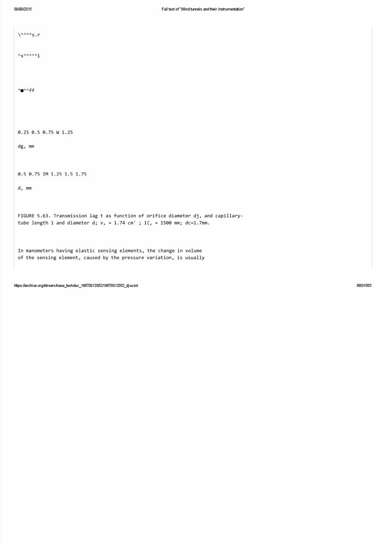
\^^^^s.r

^s^^^^^i

^■^^ff

0.25 0.5 0.75 W 1.25

dg, mm

0.5 0.75 IM 1.25 1.5 1.75

d, mm

FIGURE 5.63. Transmission lag t as function of orifice diameter dj, and capillary‐

tube length 1 and diameter d; v, = 1.74 cm' ; 1(, = 1500 mm; dc=1.7mm.

In manometers having elastic sensing elements, the change in volume

of the sensing element, caused by the pressure variation, is usually

 

so sma a can e gnore . e ma n ac ors n uenc ng e

transmission lag are the orifice diameter do, the internal diameters d of

the capillary tube and dc of the connecting tube, and their respective lengths

/ and ic .

Figure 5. 63 shows the relationships between the transmission lag and

do, d , and / for u„ = 1.74 cm^ (Figure 5. 62), d^ = 1.7 mm, and h= 1500mm

I 21 1 . Initially this system was under atmospheric pressure; the pressure

at the orifice was then suddenly reduced to 20 mm Hg. These conditions

approximate those of manometers in intermittent ‐operation supersonic

wind tunnels.

The orifice diameter is of small influence when rf/do < 2.5 . When d/do>2.5

the transmission lag increases sharply. The orifice diameter should therefore

not be less than half the diameter of the capillary tube. An increase in

orifice diameter up to the diameter of the capillary tube has little effect on

the transmission lag.

The influence of the diameter of the capillary tube is very strong. A

reduction of this diameter has as its main effect an increase in the resistance

to the flow of gas. A length increase of the capillary tube has a greater

311

■IIIIIIIIIIHIIIIIIIII I III! ■■■III!

effect when its diameter is small. Capillary tubes should therefore have

diameters as large as possible and be as short as possible.

 

The influence of the connecting tube is twofold. Firstly, the connecting

tube has the largest volume in the system, and secondly, it offers resistance

to the gas flow. When dc is small, the transmission

lag is, as in a capillary tube, increased due to this

resistance. When dc is large, the lag increases

due to the volume increase. The connecting tubes

should therefore be as short as possible. The

optimum diameter is between 1.25d and 1.50d.

At very low pressures, for instance, in wind

tunnels with free molecular flow, where the mean

free ‐path length of the molecules is large in

comparison with the cross section of the orifice

for the tube leading to the manometer, the

transmission lag can be considerable. For d = dc

the lag can be determined according to the

following approximate formula I "ill:

FIGURE 5.64. Determination

of manometer transmission lag.

I Svl

/ =

 

32u SiidH

4‐

8^\

r.d]

V2ii RT

where v is the volume of the manometer chamber. As in the case

considered above, an optimum value exists for the internal diameter

of the tube.

Liquid ‐column manometers have in most cases larger transmission lags

than manometers provided with elastic sensing elements. This is due to

the large volumes of the air, the large moving masses, the viscosity of the

liquid, and the additional volume change when the liquid flows from one leg

to the other. In well ‐type manometers the lag depends on the method of

connection. The air volume above the capillary tube in a well‐type mano‐

meter is many times less than the volume of the air in the well. Whenever

possible, the well should be at that pressure which varies less during the

process (for instance, the total pressure).

 

or e manome r c sys em s own sc ema ca y n gure . , e

transmission lag is /28/:

where

k = ‐

/ =

Pfm‐P,

tMXp

‐Iq Piin‐Pmix.

7 ^

■— „ '""‐f v^

is the time constant of the system, i. e., the time during which the pressure

p, in the manometer changes by 63.2% of the total pressure difference

 

(p = Pjjjjj) at the orifice; u„ is the volume of the air after the final pressure

equalization.

These formulas take into account the compressibility of the air in the

manometer but ignore the inertia and viscosity of the liquid.

In the second formula, Lgq is the "equivalent length" of the capillary

tube which, when there are several connecting tubes of different diameters, is

4cr^. + i^(lr^V...+z„(|^y,

312

where L\ is the length of the tube whose diameter is d,.

The time‐averaged pressure p in the manometer is

I^.

dt

 

ns ea o s va ue, we can su s u e n s ornnu a e approx ma e

value of p up to the instant / when the pressure change in the manometer

amounts to 98% of the total pressure difference:

P — ^fin 4

The equivalent area F^^, which depends on the geometry of the manometric

system, can be determined from Figure 5. 65.

Measured pressure

acting in capillary

tube

f'

\zzzzJ

F = J^

eq «

General case

 

  u es o eren ame ers

t"

F =

KH'

Measured pressure

acting on

U‐tube manometer

with legs of

equal diameter

 

 

yS ffiif ^

\,BnJf

^ef"

tti'

FIGURE 5. 65, Determination of equivalent area of a manometer.

Thus, when the pressure changes abruptly, we can assume that the

transmission lag is inversely proportional to the fourth power of the

diam.eter of the capilllary tube, directly proportional to the length of the

tube, and depends also on the volume of the air in the instrument and the

geometry of the system.

313

 

§ 24. MANOMETRIC INSTRUMENTS FOR DETERMINING

DIMENSIONLESS CHARACTERISTICS

Many dimensionless coefficients and parameters of experimental

aerodynanaics are deternained as the ratios between dimensional magnitudes.

For instance, all aerodynamic coefficients (Chapter I) are proportional to

the ratios of the forces and moments to the velocity head of the undisturbed

flow, while the Mach number is a function of the ratio between two pressures

(Chapter IV). When each magnitude entering into the nominator and

denominator of the ratio is measured independently, it is assumed that these

magnitudes refer to the same flow conditions. However, if these

magnitudes are not read off at the same instant, then, due to the fluctuations

in flow velocity or pressure in the wind tunnel, this assumption leads to not

accurately determinable errors in the calculated ratios. In naost cases

these errors can be reduced by obtaining more steady flow conditions in the

wind tunnel or using quick‐acting measuring instruments with sim.ultaneous

automatic recording of their indications. However, in some cases a better

accuracy can be achieved by measuring not each magnitude separately but

their ratio directly. Such a "coefficient meter", which is mainly a

simplified computing device, was first used by K. A. Ushakov in 1924 for

determining the aerodynamic coefficients of airfoils in the TsAGl wind

tunnel /29/.

Nowadays, aerodynamic experimental techniques are so developed that

in many large wind tunnels the coefficients are automatically calculated on

digital coraputers. The simple devices described in this section permit

automation of these calculations in those small wind tunnels and installations

where the use of computers and complicated devices for measurements and

data input is not justified.

 

ns rumen s or measur ng orce an pressure coe c en s

At low flow velocities, any of the aerodynamic coefficients c,, Cy, d, OTx,

niy, nil are proportional to the ratio of the force or moment to the difference

between total and static pressure, e. g..

The principle of measuring the coefficient of lift in a wind tunnel is

schematically shown in Figure 5. 66. The aerodynamic force V, which

acts on the model installed on the wind‐tunnelbalance, is transmitted by rod

(1) to beam (2), at whose end contact (3) is located between two stationary

contacts (4). Beam (2) is connected with lath (6) by means of link (5), which

can be moved along the beam and the lath by lead screw (7) which is turned

by servomotor (8). The force, which acts on the lever‐type manometer

consisting of bellows (11) and lever (9), is transmitted to lath (6) by

means of two levers (10) which have the same arm ratio. When beam (2)

becomes unbalanced, one of the contacts (4) is closed, servomotor (8) is

switched on, and lead screw (7) moves link (5) to the position at which the

m.oment acting on the beam, due to force Y , is balanced in its absolute value

1680 3J4

by the moment due to pressure on the bellows, which is proportional to Ap.

It is easy to see that the distance x from the fulcrum of beam (2) to

link (5), at the instant when equilibrium is attained, is

^ " Up'

where k depends on the transmission ratio of the levers and on the area of

the bellows. The weight of levers (9) and (10), link (5), the connecting rods,

and lath (6) is balanced by counterweight (13), while the weight of beam (2)

 

an e par s connec e o s a ance y coun erwe g . e va ue o

X, which is proportional to c„, can be read off from a counter connected to

the lead screw.

nGURE 5.66. Direct measurement of coefficient of lift. 1 — cod; 2— beam;

3 — contact at end of beam (2); 4 — stationary contacts; 5 — link; 6 — lath

parallel to beam C 2); 7 — lead screw; 8 — servomotor; 9— lever; 10— levers

with equal arm ratios; 11 —bellows acted upon by pressure difference ap ;

12 and 13— counterweights.

Figure 5. 67 illustrates how the dimensionless total‐pressure coefficient

// of a fan is determined. Here,

where u is the peripheral velocity of the impeller tip. The pressure Pe , which

is proportional to pu^, is created by a so‐called unit fan, rotating at the

same speed as the tested fan and operating in air of the same density /30/.

The pressure H , created by the tested fan, and the pressure p^ act

respectively on bellows (5) and bell (4), whose effective areas are F]

and f 2 . The force on the bellows acts on the left‐hand arm of lever (1).

315

Bell (4) is mounted on a carriage moving along guides (3); the force pef2,

acting on the bell, is transmitted to the other arm of the lever by means

 

o a ro er. ever s a ance w e a o ea screw , ro a e

in either direction by means of a servo system consisting of a continuously

rotating friction wheel (6) and electromagnets (7), switched in by contacts

(8). The total‐pressure coefficient H is proportional to the distance x

between the roller and the fulcrum of lever (1), which can be read off from

a scale or counter.

^77777777.

FIGURE 5.67, Determination of the total‐pressure coe\liciQXii oi & ian. 1 —lever;

2 — lead screw; 3 — guides; 4 — bell; 5 — bellows; 6 — friction wheel; 7 — electro‐

magnets; 8 — contacts.

Whenthebeamis in equilibrium, Wfio = pcF^x, whence

Pe " F\a

Since the pressure pc is proportional to pu', the value of x is proportional

to the total ‐pressure coefficient of the tested fan:

x = cor\%iH.

Similar instruments can be used for n:ieasuring pressure coefficients

when investigating the pressure distributions on bodies.

 

ns rumen s or measur ng e ac num er

of the flow

Since in high‐speed tunnels the flow characteristics depend to a large

degree on the Mach number, its free ‐stream value must be controlled

316

during the experiment. The use of a Machmeter (as instruments for

measuring the Mach number are called) simplifies experiments at high

subsonic velocities, where models are very often tested by varying the flow

velocity at constant angle of attack. This instrument is also suitable

for modern supersonic wind tunnels with adjustable nozzles. The Mach

number in the test section of such a tunnel is changed gradually by adjusting

the shape of the nozzle, and the direct measurement of M permits control

of the flow conditions in the tunnel.

The Mach number is a function of the ratio of two selected pressures pi

and p2 inthe gas (see Chapter IV). Therefore, any instrument which measures

the ratio of p, and p^ can be used as

Machmeter. The scale of such an

instrument need not be linear, since

the functional relationship M = flpilpi)

is not linear. The Mach number can

be determined from the ratio of the

total pressure po (or the pressure

difference Ap = po — p ) to the static

pressure p in the undisturbed flow.

 

e s mp es ev ce or measur ng

the Mach number is shown in Figure

5. 68. It consists of a well‐type mano‐

meter with measures Ap , and a mano‐

meter which measures the absolute

static pressure p. The zero markings

of the scales of both instruments are

interconnected by a diagonal line AB .

A string is stretched between the

moving verniers C and D . When the

verniers are aligned with the meniscuses

in the manometric tubes, the inter‐

section of lines AB and CD divides the

former into two parts whose ratio is

Ap/p. Thus, the divisions marked on

line AB correspond to values of the

Mach number, which is read off with

the aid of string CD.

Figure 5. 69 shows another device,

which permits control of the Mach

number when the pressures are measured with the aid of two pendulum‐

type manometers. When the pressure p, changes, the angle of inclination

of pendulum (1), to which a curved mirror (3) is fixed, also changes. A

light beam falls on mirror (3) from light source (4) and is reflected onto

plane mirror (5). The latter is turned around a vertical axis OO when

pendulum (2) is inclined by the action of pressure p2. The beam is

reflected from mirror (5) onto screen (6). The vertical displacenaent of

the beam is proportional to p, and its horizontal displacement to pj — p,.

The Mach number is determined from the lines M = const, drawn on the

screen.

Automatic instruments for measuring M can be divided into two

groups. The first group includes instruments which are simple electrical

 

FIGURE 5,68. Liquid‐column Machmeter.

317

analog computers, while the second group includes instruments which are

based on force ‐balancing principles. In instruments of the first group, the

Pi P,

nGURE 6.69. Optical Machmeter with

pendulum‐type manometers. 1 and

2 — pendulum type manometers; 3 —

curved mirrori 4 — light source; 5 —

plane mirror; 6 —screen.

input into the conaputer is formed by magnitudes proportional to the

pressures pi and p^ which are measured by separate nnanometers. Automiatic

self ‐balancing nnanometers, whose output is an angular displacenaent of the

 

FIGURE 5.70. Determining the Mach number

with the aid of a balanced bridge. 1 — servo‐

motors or selsyn receivers connected to self‐

balancing manometers; 2 — amplifier ( zero

indicator); 3 — balancing servomotor; 4 —

resistor with scale for M .

FIGURE 5.71. Potentiometric deter‐

mination of Mach number. 1 and

2 — selsyn receivers connected to

manometers measuring p and ap ; 3 —

automatic potentiometer.

servomotor shaft, are most suitable for this purpose. Figure 5.70 shows

a wiring diagram used in the automatic computation of M with the aid of a

318

balanced bridge, in which the resistances of two arms are changed in

proportion to the indications p and Ap of the manometers. The other two

bridge arms are formed by a constant resistance R<i and a variable

resistance /?<. The bridge is balanced by varying the resistance /?» with the

 

a o a a anc ng servomo or w c moves e con ac o e res s or n o

the position which corresponds to the balancing of the bridge, so that

R, _ R,

R, Ri

whence

R^ = k^=.k[{l+^Mf''‐^]‐

If the resistance Rt varies in proportion to the displacement x of the

contact of the resistor and the counter connected to it, then x is linearly

related to the pressure ratio and nonlinearly to the Mach number. The

scale from which M is determined is thus nonlinear. For x to be proportional

to M, it is necessary that the following relationship exist between the

resistance and the displacement of the contact:

/?4 = a[(

where ‐k andjfci, are constants.

1 +

 

I— I

M)"‐'‐iJ

l.€

0.S

"IT 0.6

0.8

a‐l

u/x/

YMA

02 OM 0.6 0.6

 

1.0

a‐05

\

y

\

^^

 —

^

 

i^

Y

/•'

0.Z O.'i 0.6 0.6 1.0

FIGUflE 5.72. Output voltage of potentiometric system as function of Mach number.

Figure 5. 71 shows the wiring diagram, of a computing device based on the

 

pr nc p e o e po en ome er. cons an vo age ua orms e npu o

the potentiometer which consists of two variable resistances /?, and /?,. The

output voltage ui is a function of the ratio of the resistances i?i and i?2. If

the resistances R^ and ^2 vary in such a way that /?, = kip and R^ = AjAp , then

[ui = uo/(/ + k\plki^p)\ and UjWill therefore depend only on the Mach number.

The output voltage can be measured with high accuracy by the null method,

for instance, by an automatic electronic potentiometer. By changing the

raio ft, /As the function u, =/(M) can be varied considerably. Thus, for

instance, for fti/*2 = 0.5 , the output voltage changes almost linearly with the

Mach number in the range 0.3 < M < 1 . The linearity can be improved if the

319

resistance R, and R2 change with the pressure in such a way that

Ri= fiiP' and Ri — k^l^p'.

In this case the functional relationship between «i and the pressure

ratio is

„ "0

By varying a. , we obtain different functional relationships, so that in

different parts of the Mach ‐number range linearity will be maintained as

closely as possible. Figure 5, 72 shows that for ktjkz = 5 and a = 0.5 we

obtain a relatively high linearity in the entire range 0<M<l/32/.

 

‐| Manometer zE‐

(Machmeter) P

Flow‐velocity mea‐

suring bridge " V "

FIGURE 6.73. Determination of the Mach number with the aid of electro‐

magnetic manometers and of the flow velocity with the aid of a resistance

bridge. 1— 1'‐ lever‐type manometers; 2— 2' ‐transducers; 3 —

3' '‐ coils; 4 — . 4' ‐ permanent magnets; CM^ , Cm, , CM, ‐ servo‐

motors; y„ y, H y,‐ amplifiers.

Figure 5, 73 shows the wiring diagram of a manometric system which

permits the Mach number and the actual flow velocity to be measured

320

simultaneously. The system consists of two electromagnetic lever ‐type

manometers and a comiputing device in the form of an automatic m.easuring

bridge. One manometer serves for measuring the absolute static pressure

p. When p changes, the equilibrium of lever (1) is disturbed, and transducer

(2), through amplifier Vi, switches on servomotor CM, which, with the aid

 

o var a e r eos a , c anges e curren n ens y , n co . e

latter is fixed to the lever, and the variation in current intensity causes the

force of interaction between the magnetic fields of the coil and the permanent

magnet (4) to change in such a way that lever (1) returns to its equilibrium

position. The current, which is proportional to p, can be measured by the

position of the shaft of the servomotor CMi or of the slider of the rheostat Pi.

A second manometer differs from the first only in that its balancing coil

(3'), connected to lever (1'), is acted upon by electromagnet (4'), whose

winding is connected in series with coil (3). Hence, the force of interaction

between coil (3') and electromagnet (4') is proportional to the product of the

current intensities i, and ij. Lever (1') is acted upon by a moment which is

proportional to the pressure difference Ap. When Ap changes, transducer

(2'), through amplifier (y2), switches on servomotor CAf2, which moves the

slider of the variable rheostat Pj. This alters the current intensity ij in

the circuit of coil (3'), and restores lever (1') to its equilibrium position.

Since i, is proportional to p, the current intensity I'j at the instant when lever

(1) returns to its equilibrium position depends only on the pressure ratio:

1 = const ‐^=/(M);

the second manometer is therefore a Machmeter,

The device for com.puting K is a four‐arm bridge, two of whose arms

are formed by resistances /?i and /?2. The magnitudes of the latter are changed

by servomotor CM^ simultaneously with that of rheostat P2. The third arm

of the bridge consists of a resistance thermometer in the settling chamber

of the wind tunnel. The magnitude of this resistance is

'■<o = '‐oIl+«(7"o‐ 273)1,

where ro is the resistance of the thermometer at 0°C, a is the temperature

coefficient of the resistance, and To is the stagnation temperature of the

gas. The resistance no is connected in series with a constant resistance

which has a negligibly small temperature coefficient, and is equal to

 

  = ■ — a . ence, e o a res s ance o e arm w e

^3 = '""oT'o‐

When the supply voltage u of the coils is constant, the rotation angle

of the shaft of servomotorCAfj and the displacements of the sliders of

rheostats /?i and R2 are proportional to Ap/p. The resistances Ri and R2,

which vary with the displacements of the sliders, can be chosen in such a

way that they are proportional respectively to

M^and i + ^^M^.

321

The bridge is balanced by servomotor CM3 which is fed from amplifier

(null indicator) Y3. When the bridge is balanced.

R,

M'

i + ‐

 

‐M2

whence

/?4 = ‐

arjTjM^

1 + ‐

‐1

M=

The actual flow velocity is expressed through the Mach number and the

stagnation temperature:

 

  =

v.gRT„M'

1 + ^

M^

Since for a given gas x and R are constant, Ra is proportional to V''. If Rt

varies like the square of the slider displacement, the rotation angle of the

shaft of servomotor CM3 will be directly proportional to the actual flow

velocity.

In all these instruments one or both pressures entering into the functional

relationship M = [(Pi/Pi) are measured independently, so that the Mach number

is determined indirectly.

Vacuum

•jww7w//y/}///yy////y/y///^(/'//'/y'/////'///////, v///\'//a vtz.

 

  . . ec romec an ca ac me er. an — evers; an — xe

knife edges; 5 — movable knife edge; 6 — lead screw; 7 —servomotor; 8— transducer;

9 —counter; 10 —counterweight.

Figure 5. 74 shows an electromechanical device which directly measures

the ratio of two pressures, i. e., permits the Mach number to be found

directly. The advantage of such devices is that there is no need to balance

each pressure separately. The device consists of two levers (1) and (2),

resting on fixed knife edges (3) and (4). Each lever is connected to a pair

322

of bellows, acted upon by the total pressure, static pressure, and vacuum

in such a way that the moments of the pressure forces, about the fulcrums

of levers (1) and (2) are proportional to Ap and p respectively. These moments

are balanced by the moment of the reaction A/ of movable knife edge (5), which

connects levers (1) and (2). The position of knife edge (5) can be changed with

the aid of lead screw (6), which is rotated by servomotor (7). The change in the

moment about the fulcrum of lever (2), of the weight of knife edge (5) when the

latter is displaced, is compensated by moving counterweight (10), in the

opposite direction.

For this purpose part of lead screw (6) has a left‐hand thread. When

the equilibrium of the levers is disturbed by a pressure variation, the

servomotor is switched on by transducer (8) and moves knife edge (5) into

a new position at which the equilibrium of the levers is restored. The

equilibrium condition is given by

 

Nx = Ap/^ifl

_ .^‐1

L — x

77 Pt<^<

where L is the distance between knife edges (3) and (4), while f and a

with corresponding subscripts are the effective areas of the bellows and

the distances between their center lines and knife edges (3) and (4),

respectively. When the static pressure is equal to the total pressure ,

i. e., when the flow velocity is zero, lever (1) exerts no force on lever (2),

because in this case the reaction N passes through the fulcrum of lever (1),

The initial position of knife edge (5) is in line with knife edge (3), its

displacement from this initial position being

x^L

k + hpip

 

where k= /— is constant.

Thus X is a function of the Mach number which can be determined with

high accuracy from the indications of counter (9), which is connected to

lead screw (6).

10

0.5

^

 

=

^

*

»'

 

 

.^

‐‐

^

i

/

/

/

 

/'

y

■'

•

^

k‐

V'

/

 

 

/

/

/

,/

X

 

 

i

A

/

/

/

/

'

A

 

/

V

^

y

 

/K'W

y

y

 

^

 

1.0

10

3.0

FIGURE 5.75. Dependence of relative knife‐edge displacement on Mach

number.

323

Figure 5. 75 shows the dependence of the relative displacement xlL

on the Mach number. By selecting different values of k, we can obtain

maximum sensitivity of the instrument dx/dM for different sections of the

Mach ‐number range. In practice^ use of the instrument is limited to the

range 0.5 < M < 3 , since for M> 3 the static pressure p drops very sharply

and the accuracy of the instrument is reduced due to the small displacements

of knife edge (5), required to restore the system to its equilibrium

position.

 

Bibliography

1. Deshman,S. Nauchnye osnovy vakuumnoi tekhniki (Scientific

Basis of Vacuum Technology). [Russian translation. 1950. ]

2. Spravochnik kJtiimika (Chemical Handbook). — Goskhimizdat. 1951.

3. Farquharson,J. and H. A. K e r nikl e . Precise Automatic

Manometer Reader. — Rev. Sci, Instr., Vol. 28, No. 5. 1957.

4. Zhukova, L. A., N. A. Kolokol o va , and V. A. Sukhn e v .

Izmerenie malykh perepadov davleniya v razrezhennykh gazak

(Measurennent of Small Pressure Drops in Rarified Gases). —

Izvestiya AN SSSR, OTN, Mekhanika i Mashinostroenie, No. 6.

1961.

5. Falkner.V. M. A Modified Chattock Gauge of High Sensitivity. —

ARC Rep. and Mem. 1589.1934.

6. MacMillan^F. A, Liquid Micromanometers with High Sensitivity

and Small Time Lag. — J. Sci. Instr., Vol. 31, No. 1. 1954.

7. Smith, A. and J. S. M ur phy . Micromanometer for Measuring

Boundary Layer Profiles.— Rev. Sci. Instr. Vol.26, No. 8. 1955.

8. Hart,H.R. Electric Micromanometer. — J. Sci. Instr., Vol.38,

 

No. 7. 1961.

9. Midwood,G.F. and R. W. Hay w ar d . An Automatic Self ‐Balancing

Capsule Manometer. — ARC Cur. Pap., No. 231. 1956.

10. Kinkel, J.F. A Precision Pressure Balance. — Proc. Instr. Soc.

Am., Vol. 7. 1952.

11. Op St el t en , J. J. and N. Wa r m ol t z . A Double‐Sided Micromano‐

meter.— Appl. Sci. Res., B 4, No. 5. 1955.

12. H all i day , A. S. and H. Deacon. A Distant Reading Manometer for

Particular Application to the Measurement of Small Pressures. —

ARC Rep. and Mem., No. 2744. 1952.

13. Neubert, N.K.P., W. R. M a c donal d, and P.W.Cole. Sub‐

Miniature Pressure and Acceleration Transducers. — Control,

Vol.4, No. 37. 1961.

14. Pressey, D. C. Temperature‐Stable Capacitance Pressure Gauges. —

J. Sci. Instr., Vol.30, No. 1. 1953.

15. Cook, D.B. and C. J. Danby. A Simple Diaphragm Manometer.—

J. Sci. Instr., Vol.30, No. 7. 1953.

16. Wrathall,T. Miniature Pressure Cells. — Proc. Instr. Soc. Am.,

 

Vol. 7. 1952.

17. Bassiere, M. Une manometre differential miniature. — Technique

et science aeronautique, No. 3. 1956.

324

18. Delmonte,J. A Versatile Miniature Flush‐Diaphragm Pressure

Transducer. — Proc. Instr. Soc. Am., Vol. 7. 1952.

19. Molyneux.W. Measurement of the Aerodynamical Forces on

Oscillating Aerofoils. — Aircraft Engg. 28, 232. 1956.

20. Wuest,W. Vielfach‐Registrier‐Manometer fiir langsamverander‐

liche Driicke in der Stromungsmesstechnik. — ATM, Lief. 271.

Aug., 1958.

21. Taudler,W.S. Automatic Instunaent for Reading Bourdon Gages. —

Rev. Sci. Instr., Vol.27, No. 2. 1956.

22. Campbell, P. J. A Multiple Recording Manometer. — J. Aero. Sci.,

Vol. 10, No. 8. 1943.

 

. ar er, . . an . . emp e r on . cann ng a ve pee s p

Pressure Plots. — Aviation Age, Vol. 26, No. 4. 1956.

24. Sharp, E.M. A Digital Automatic Multipoint Pressure‐Recording

System. — Proc. Instr. Soc. Am., Vol. 7. 1952.

25. Bain,M. and M. Seamons. Economical On‐Line Data‐Reduction

System for Wind‐Tunnel Force and Pressure Tests. — IRE

Transact, on Instrumentation, Vol. 1‐7, No. 2. 1958.

26. Wood,M.B. and J. N. W. Baldwin. Digital Recording in Multipoint

Pressure Surveys. — Control, Vol. 3, No. 21. 1960.

27. Dyukov, A. Inertsiya izmeritelei davleniya v sverkhzvukovykh

aerodinanaicheskikh trubakh (Transmission Lag of Pressure

Meters in Supersonic Wind Tunnels). — "Mekhanika" No, 1,IL. 1955.

28. Benedict, R. P. The Response of a Pressure‐Sensing System. —

Trans. ASME, J. of Basic Engng., Vol. 82, No. 2. 1960.

29. Ushakov, K. A. Novyi metod izmereniya sil pri aerodinamicheskikh

ispytaniyakh (New Method for Measuring Forces during Aero‐

dynamic Tests). — Trudy TsAGI, No. 5. 1924.

30. Ushakov, K. A. Metod neposredstvennogo polucheniya bezrazmernykh

kharakteristik ventilyatorov (Method of Directly Determining

 

on mens ona arac er s cs o ans . — n; orn

"Promyshlennaya aerodinamika". No. 17, Oborongiz. 1960.

31. Schaaf,S.A. andR.R. Cyr. Time Constants for Vacuum Gage

Systems. ‐J. Appl. Phys., Vol.20, No. 9. 1949.

32. Manaldi,I.F. Mach Number Measurement. — ISA Journal, Vol.2,

No. 4. 1955.

325

Chapter VI

WIND‐TUNNEL BALANCES

The aerodynamic forces and moments acting on models tested in wind

tunnels can be determined indirectly by naeasuring the pressures at many

points of the model surface. A more accurate and reliable method is the

direct measurement of the forces and moments with the aid of wind‐tunnel

balances.

In contrast to ordinary scales, which serve to measure forces acting

in a known direction, wind‐tunnel balances must measure not only

aerodynamic forces, the direction of whose resultant is unknown, but also

the moments about certain axes, due to this resultant and to couples. In the

most general case, wind‐tunnel balances must measure the components of this

resultant (called total aerodynamic force), along three mutuallyperpendicular

axes passing through an arbitrary point, and the three components of the

total moment about these axes (Figure 6. 1). The peculiarity of an

 

aero ynam c exper men s a n e process e magn u e an rec on

of the total force and the moment can change; in the design of wind‐tunnel

balances this has to be taken into account.

Having determined the projections of the total aerodynam.ic force and the

moment in the coordinate system of the given wind‐tunnel balance, we can

transform them into another coordinate system., whose origin can be placed

at any desired point, for instance, at the center of gravity of the airplane

or rocket.

The main characteristic of wind‐tunnel balances is the number of

measured components. Depending on the problem considered, this number

can vary from. 1 to 6. The design of the balances must provide the

possibility of measuring and altering the angle of attack, and in many cases

also of the slip angle of the model. When solving a two‐dimensional

problem, for instance, for a symmetrical model of an airplane at zero

slip angle, three ‐component balances are used, which measure the lift,

the drag, and the pitching nnoment. In this case the balance must have a

m.echanism permitting only the angle of attack to be changed. When

problems connected with lateral control of flying missiles are investigated,

four ‐component balances are used which permit also the angle of heel to

be measured. In certain partial problems single‐ and two‐component

balances are used, most often for measuring drag and lift or one component

of the moment.

Depending on their location, wind‐tunnel balances can be divided into

two types: balances located outside the model and the test‐section of the

wind tunnel, and balances located inside the model or its supports. In the

326

 

balances of the first type, the total aerodynamic force and moment are

resolved into components with the aid of various mechanisms. These

balances will be called mechanical balances. The model is installed in

the test section of the tunnel with the aid of supports connected to these

mechanisms. The supports are also acted upon by aerodynamic forces

and moments whose values have to be taken into account when determining

the true aerodynamic forces and moments acting on the model. In addition,

it is necessary to take into account the interaction (interference) between

the supports and the model, caused by flow perturbation near the model

due to the presence of the supports. Methods of determining the influence

of the supports are described in Chapter VII.

FIGURE 6. 1. Coordinate axes and projections of aerody‐

namic loads acting on the model. The broken lines re‐

present the flow system of coordinates xyz. The full

lines represent a coordinate system fixed to the model.

The .r'‐axis belongs to the semifixed coordinate system

In many cases, especially at large flow velocities, the drag of the

supports can be considerable and lead to large systematic errors.

Hence, reducing the drag of the supports is very important, and the

design of the wind‐tunnel balances depends greatly on the type of support.

In "external" (mechanical) wind‐tunnel balances the components of

forces and moments are usually determined in a system of "balance" axes

parallel to the flow axes of coordinates. Some low‐speed tunnels have

revolving frames which serve to alter the slip angle of the model; the

indications of such balances refer to semifixed coordinate axes.

 

The drawback of mechanical wind‐tunnel balances is the comparatively

high weight of their elements; due to the inertia of the measuring system

such balances cannot be used in tunnels having short operating durations.

Wind‐tunnel balances located inside the model enable the influence of

the supports to be excluded almost completely at supersonic flow velocities.

The small dimensions of the models tested in supersonic wind tunnels do not

permit mechanical balances to be placed inside the miodels. Practical

327

■I

designs of "internal" wind‐tunnel balances became possible only with

the development of strain‐gage measurement methods during the past

two decades.

Methods of measuring forces by strain gages are based on the use of

elastic systems whose deformations (which are proportional to the

mechanical loads, and therefore to the forces and moments) are determined

with the aid of small strain gages. The latter emit electric signals whose

values are simple functions of the forces and moments. Using different

electric diagrams, we can convert these functions so as to obtain signals

which are proportional to the components of the aerodynamic forces and

moments.

At present, balances placed inside the models are widely used in high‐

 

spee w n unne s. no er a van age o w n ‐ unne a ances ase on

strain‐gage principles is their rapid response, which permits measurements

of forces in tunnels in which steady flow lasts only tenths of second.

§ 25. WIND‐TUNNEL BALANCES LOCATED

OUTSIDE THE MODEL

In spite of the many different designs of mechanical wind‐tunnel

balances, there are several elements which are common to most types.

These elements are: the supports for the model; the floating frame for

holding the supports and for taking up the forces acting on the model; the

mechanical system for resolving into components the forces taken up by

the floating frame, and balance elements or dynamometers connected to the

output links of this system; and mechanisms for changing the angle of

attack and the slip angle of the model.

According to the design of the devices supporting the model, we

distinguish between balances with rigid and with flexible model supports.

In balances with rigid supports the model is secured to the floating frame

with the aid of rigid supports or struts. In balances with flexible supports

the model is secured with the aid of wires, strings, or tapes tensioned with

the aid of auxiliary weights or springs. In several designs the separate

links of the flexible or rigid supports form the elements of the mechanical

system for resolving the aerodynamic force into components. In this case

no floating frame is required as a separate element.

The tested model is very often installed in a reverse position in the

test section of the wind tunnel so that the positive lift is added to the weight

of the model and the floating frame. In this case the balance is placed

above the test section. The weight of the floating frame is chosen in such

a way that at the maximum negative value of the lift, the hinges and links

of the mechanism will be subjected to a certain load, so as to maintain

 

em n con ac .

Models in the true ("flying") position are installed in large wind tunnels.

In such tunnels the weight of the tested models is large and it is good

practice to increase the accuracy of measurements by partly unloading

the floating frame of the lift acting upward. In addition, placing the

balance above the test section when the latter is large complicates the

design of the supporting devices for the balance .

328

The aerodynamic forces and moments taken up by the model and

transmitted to the floating frame (or to elements replacing it), are measured

by determining the reactions necessary to prevent translational and rotary

displacement of the model. This is done by force‐measuring instruments

(balance elements or dynamometers) in the links of the system for resolving

the force into components, which usually consists of a multi‐link articulated

mechanism. The links must be designed so as to reduce to a minimum the

work done by friction during the displacments. A number of non ‐Soviet wind

tunnels are provided with hydraulic and pneumatic mechanisms for

resolving the forces into components; they consist of kinematic pairs with

very low friction.

For better utilization of the wind tunnel and to speed up the tests, it is

desirable that the forces be measured on the balance as quickly as possible.

This is made possible in modern wind tunnels by using special balance

elements with automatic equilibration and recording of the indications.

In order to determine the dimensionless aerodynamic coefficients, it is

necessary to measure, simultaneously with the forces acting on the model,

 

e parame ers rom w c e ve oc y ea can e e erm ne see

Chapter IV).

The simultaneous measurement of all force and moment components is

very important for the accuracy of the experiment. In several old designs

of balances, which today have only historical interest, each component was

measured separately. The accuracy of determining dimensionless

coefficients by measuring forces at different instants is reduced, for

instance, because of possible variations of the velocity head between

readings. The dynamical characteristics of all balance elements should

be uniform and close to those of the instruments used for measuring the

flow parameters.

One of the most cumbersome operations when preparing the experiment

is the mounting of the model and its supports. In a modern wind tunnel

this takes far more time than the measurements. The tendency in

designing the supports is to provide maximum ease of model installation

and interchangeability of parts and sub‐assemblies. In several industrial

wind tunnels, two or three sets of balances are provided to speed up

replacement of the model. While one set is used for the experiment,

different models are mounted on the other sets. In supersonic tunnels, each

set of balances is installed in a separate test section provided with wheels

and carried on rails. Replacing the test section requires less work than

exchanging the model.

Mechanism for resolving the forces

into components

Depending on the method of resolving the forces into components, wind‐

tunnel balances can be divided into two groups:

1. Balances in which the loads taken by one or several elements depend

 

on wo or more componen s.

2. Balances in which each element takes up a load which is proportional

to only one component.

329

Balances of the first group have a simpler system for resolving the

forces into components than those belonging to the second group. In

balances of the first group the loads taken up by the elements are functions

of the sums or differences of two or more components. Some calculations

are required to determine the separate components; this makes observation

of the experiment difficult. In some earlier designs of such balances,

several magnitudes were measured separately, while after each

measurement certain naanipulations with the balance mechanism were

necessary. Such were, for instance, the balances based on the three ‐

moment principle, used in N. E. Joukowski's laboratory at the University

of Moscow and in the Eiffel Laboratory in France. In these balances, the

mom.ents about three points of the floating frame to which the tested model

is secured are measured successively. Solving equatations of statics, the

drag Q, the lift Y, and the pitching moment M^ are then determined.

In balances of the second group, each element is intended for measuring

a separate component. These balances require more com.plicated

naechanisms for resolving the forces into components, but their advantage

is the simplicity of processing the results of measurements and the

possibility of directly controlling the experiment. This is most important

in modern high‐power wind tunnels, in which maximum reliability of

experimental results is aimed at.

 

o s mp y e con ro o e exper men w en us ng a ances o e rs

group, primary automatic processing of the measurements is sometimes

employed. This processing consists of algebraically summimg up

indications of separate elements, resulting in "net" values of the components.

For all designs of mechanical wind‐tunnel balances it is possible to

deduce general conditions necessary for the independent measurement of

each component by one balance element. These conditions are that the

work done by the component of the total aerodynamic force or moment

over the corresponding displacement of the model must be equal to the

work done by the force acting on the balance element over the measuring

distance of the latter. In the absence of friction in all kinematic pairs, and

of deformation of the links in the mechanism which resolves the forces

into components, we obtain

Nm/m,‐

‐yM,5, = 0,

Nm/m^. ‐

‐M,5s=a

Nm/m,'

 

‐ yw,6, = 0.

Here 8«, 5y, 5, are the possible translational displacements of the model

parallel to the coordinate x, y , and ?‐axes, 8^, 5^ 6^ , are the possible

rotations of the model about these axes, Ao , Aaj^, are the displacements

of the input links of the balance elements, and A'^, . . . , N^ , are the loads

acting on the latter.

Kinematically these conditions mean that for a small translational

displacement of the model parallel to any axis, there must be a motion,

parallel to its axis, only of that link which connects the balance system

with the element intended to measure the force component acting in the

direction of the axis considered. For a small rotation of the model about

any axis, only that link must move parallel to its axis, which connects the

system with the element intended to measure the moment about said axis.

330

If we disconnect the balance elements from the mechanism resolving

the forces into components, the model will have a number of degrees of

freedom, equal to the number of the measured components. Each element

is connected to such a point of the mechanism that when the latter is fixed

the model is deprived of only one degree of freedom. Thus, if all the scale

elements were absolutely rigid and fixed (i.e., the link taking up the force

did not move under the action of the force), the system for resolving

 

e orces n o componen s wou ecome a s a ca y e erm ne sys em.

''*,. Y r

m

rrtujfinfjf^ffn

a)

b)

FIGURE 6.2. Parallelogram mechanisms for measuring forces, a — measurement of q ;

b ‐ measurement of k ; c — measurement ofQ and Y.

 

Thus, the components can be measured independently by using

mechanisms which permit free translational displacements of the model,

parallel to the coordinate axes, for measuring forces, and free rotational

displacements about the coordinate axes, for measuring moments. The

number of degrees of freedom of the mechanism must be equal to the

number of the measured components. Such systems can be formed from

a number of elementary mechanisms : mechanisms for translational

displacements, mechanisms for rotational displacements, and combined

mechanisms .

Mechanisms for translational displacements. The

simplest mechanism for measuring forces, which is widely used in wind‐

tunnel balances, is a hinged four‐link mechanism forming a parallelogram.

Figure 6. 2 shows balances for measuring the drag Q and the lift Y with the

aid of parallelogram mechanisms. The floating frame is connected to

rods AC and BD, whose direction is perpendicular to that of the measured

force and which are hinged at C and D respectively. By means of the rod

AE , which is parallel to the direction of the measured force, the floating

frame is connected directly (or through a lever transmission which is not

shown) with the corresponding balance element (BEq, BEy).

At a small displacement of the hinge E along AE , the frame AB together

with the model moves parallel to the direction of the drag Q (Figure 6. 2a)

331

or the lift Y (Figure 6. 2b). In these displacements, work is done only by the

force components Q and Y respectively; they are thus measured

independently of each other and of the pitching moment. If we measure

 

e orces an ac ng n e ro s an y separa e e emen s,

the indications of these elem.ents enable us to determine the moment M^

about any axis perpendicular to the xy plane. However, if the hinges C

and D are displaced in the direction of the rods AC and BD, work is done

(by the forces Y and Q in Figure 6. 2a or the force Q in Figure 6. 2b, and

the naoment M. ); the balance elements connected with these rods would

thus measure forces Wi and N2 depending both on the components of the

total force and on the moment. In this case the values of Y (or q) andAfj

can be determined from the indications of two or three balance elements

by solving the corresponding equations given in the figure.

By combining two parallelogram mechanisms, we obtain a mechanism

which permits independent measurement of two orthogonal forces

(Figure 6. 2c). This system employs, in addition to the main floating

frame to which the model is secured, a rigid auxiliary floating frame to

which the rods are hinged.

When measuring the horizontal forces with the aid of parallelogram

mechanisms, a small ratio of the horizontal force AQ to the horizontal

displacement Op of the floating frame, caused by it, is inaportant; ( Jq is

reckoned from the zero position at which the rods AC and BD are vertical

and perpendicular to AB (Figure 6. 2a). The force AQ represents the

horizontal components of the forces /V, and A'2 induced by the weight of the

floating frame in rods which are inclined at an angle of Sp/a . If the

weight of the floating frame is G while the length of the rods AC and BD

is a, then when 5p is small^

whence

AQ^iN, + N,)^^G^

 

AQ_

It follows from this that the sensitivity of the system measuring the

force Q can be increased by lengthening the rods or reducing the weight

of the floating franae.

When the floating frame is heavy, high sensitivity of the parallelogram

mechanism can be achieved only through long rods which require a high

room for installing the wind‐tunnel balances. The "antiparallelogram"

support of a floating frame (Figure 6.3a) increases the sensitivity when

short rods are used. The translational displacement of the frame is

obtained by hinging it at O, and O2 to the equal‐ arm levers P, and Pj linked

tovertical rods (1), (2) and (1') and (2'). The sensitivity is increasedby the

forces in rods (1) and (2) (and also in (1') and (2')) having different signs;

when the floating frame is displaced, the horizontal projections of the

forces in the inclined rods act pairwise in opposite directions. For

the antiparallelogram support we have

332

where a, and a2 are respectively the length of rods (1) and (2) (or (1') and

(2^)). If rods (1) and (2) are of equal length the sensitivity is infinitely large.

 

, .‐ . n.

■/■^rrrrrrr^f irf^ ^.•rrj^^fTTTTryrm

0‐:at« ‐T‐ G

FIGURE 6.3. Measurement of drag Q . a — with the aid of antiparallelograms ; b —

with the aid of Chebishev mechanisms .

In a parallelogram support this is possible only with infinitely long rods.

Figure 6. 3b shows a system which provides translational displacement

of the floating frame with the aid of Chebishev mechanisms, in which the

equal‐arm levers P| and P^ are carried by inclined crossed rods. The

advantage of this mechanism is in that the lift on the model and the weight

of the floating frame act on rods (1) and (2) (or (1') and (2')) in the same

direction. This facilitates the design of the hinges.

^7777777777777777777777

a)

 

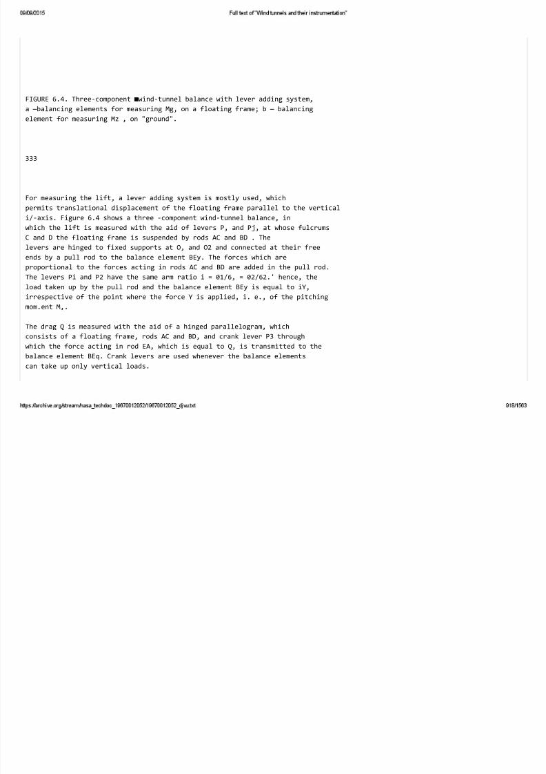
FIGURE 6.4. Three‐component ■wind‐tunnel balance with lever adding system,

a —balancing elements for measuring Mg, on a floating frame; b — balancing

element for measuring Mz , on "ground".

333

For measuring the lift, a lever adding system is mostly used, which

permits translational displacement of the floating frame parallel to the vertical

i/‐axis. Figure 6.4 shows a three ‐component wind‐tunnel balance, in

which the lift is measured with the aid of levers P, and Pj, at whose fulcrums

C and D the floating frame is suspended by rods AC and BD . The

levers are hinged to fixed supports at O, and O2 and connected at their free

ends by a pull rod to the balance element BEy. The forces which are

proportional to the forces acting in rods AC and BD are added in the pull rod.

The levers Pi and P2 have the same arm ratio i = 01/6, = 02/62.' hence, the

load taken up by the pull rod and the balance element BEy is equal to iY,

irrespective of the point where the force Y is applied, i. e., of the pitching

mom.ent M,.

The drag Q is measured with the aid of a hinged parallelogram, which

consists of a floating frame, rods AC and BD, and crank lever P3 through

which the force acting in rod EA, which is equal to Q, is transmitted to the

balance element BEq. Crank levers are used whenever the balance elements

can take up only vertical loads.

 

FIGURE 6.6. Method of removing excessive degrees of freedom of a floating

frame

Figure 6, 5 shows a method for rennoving excessive degrees of

freedom, in the directions of the components not measured, of a floating

three ‐component frame. For this purpose, the adding lever P2 has two

equal horizontal arms of length 02, which are connected to each other

and to the central arm (of length 62 ) by a rigid transverse element. The

lever Pj can rotate about axis O2OJ , at the same time preventing the

floating frame from rotating about any axis parallel to Ox . The crank

lever P3 which has two equal arms of length C, also interconnected by a

rigid transverse element, adds the forces acting on the rods AE and A'E'

which are parallel to the x‐axis, and transmits the load, which is

proportional to the drag Q, to the balance element BEq, This lever prevents

334

the frame from rotating about any axis parallel to Oy. Trans lational

displacement of the frame in the direction parallel to the z‐axis is

prevented by a hinged rod 00 which connects the frame to a fixed support.

Mechanisms for measuring moments. The transverse axis

Oz of wind‐tunnel balances is usually the axis about which the model rotates

when its angle of attack is altered. Hence, at all angles of attack, the

origin of the balance coordinate system remains fixed in relation to the

model. When the model is sufficiently large it can be hinged along the

 

z‐ax s o e xe par o e suppor . e a sec on o e mo e as

hinged to it a movable streamlined strut by means of which the angle of

attack is altered.

Mechanisms for measuring moments can be divided into two groups:

mechanisms with measuring hinges on the model and mechanisms without

measuring hinges. Measuring hinges are bearings on the supports with

whose aid the angle of attack of the model can be altered, while at the same

time a slight rotation of the model, at low friction, enables a force to be

transmitted through the tail strut to a balance element which measures the

pitching moment M,. An example of a three ‐component balance with a

measuring hinge on the model is shown in Figure 6.4a. The pitching

moment M, is measured with the aid of lever Pj and balance element BE^,

supported on the floating frame AB .

FIGUE^ 6.6. Load distribution on hinges of model supports.

335

The pitching moment is transmitted to lever p^ by strut T, hinged to

the tail section of the model and to an intermediate lever P^. Rotation

of the latter about support O4 of lever Pi causes the angle of attack of

the model to be altered.

 

«

FIGURE 6,7, Six‐component balance with measuring

hinges on the model.

If, in addition to the pitching moment M,, the components M^ and My have

to be determined, the measuring hinges have two or three steps. The

model, which is fixed to the supports at three points, can in this case be

considered as a three‐dimensional statically determined beam supported

at three points (Figure 6. 6). The components of the total aerodynamic

moment cause reactions at the hinge supports O, and O2, which can be

geometrically added to the reactions at these supports, caused by the

components of the total force.

A six‐component balance /2/ with measuring hinges on the model is

shown in Figure 6. 7. The model is supported at points d and O2, which are

located at a distance a from each other (transverse base) in the wings of the

model, bynieansof wires or tapes connected to two separate floating frames

Fi and F,. The tail hinge O3, located at a distance / (longitudinal base) from

336

the line 0, O^ (the z ‐axis), is connected by a wire or tape to the lever P,

whose rotation in relation to a lever Pj indicates the angle of attack of

the model. Levers P, and P^ are connected by means of a worm gear.

Lever Pi transmits the load due to the pitching moment Mt, to the balance

 

e emen y .

All vertical components acting at Oi, O2 and O3 are transmitted to balance

elements B£r,, B£y, and B£y, respectively through levers having equal

transmission ratios i^ . The horizontal components acting at Oi and O2,

which are parallel to the jc‐axis, are transmitted to balance elements BEq,

and B£q, through crank levers whose transmission ratio is (q, while the side

force Z is transmitted to balance element BE^ through a crank lever having

a transmission ratio i^ . If we denote the loads taken up by the balance

elements by N with the corresponding subscript, the different components

of forces and moments are:

Q =

iQ{NQ,+NQ,),

Y =

iy{N„ + Ny.+ Ny,)

Z =

izN^,

M.=

 

ha(JV„‐N,,).

M,=

iqlliNQ, — Nq,),

M,=

iylNy,

In order to permit negative values of M^, M, and Y to be measured,

the balance elements BEy, BEy, and B£i‐, are preloaded by weights G.

99

«?«,

9

^"‐^

 

p‐

FIGURE 6.8, "Pyramidal"* support for floating frame.

337

The design of this balance does not permit independent measurements of

the components. The above fornnulas show that only Z and M^ are

determined as the indications of a single balance element. The other

force components are deternnined as sums, and the other moment

components, as differences of the indications of balance elennents.

Measuring hinges are comparatively easily installed on models of wings

tested in subsonic wind tunnels. When models are tested at high flow

velocities, it is extremely difficult to install the measuring hinges, because

of the small dinaensions of the model and the large loads . Transonic and

supersonic wind tunnels often have, therefore, balances in which the

instantaneous axes of rotation of the model coincide with the coordinate

axes of the balances without measuring hinges being provided on the model.

 

Differing in design from balances with measuring hinges, where

displacements of the balance elements measuring the moments are caused

by displacements of the m.odel in relation to its supports, in balances with‐

out measuring hinges, displacements of the balance elements are caused

by displacements of the m.odel together with its supports. An example

of such a design, the so‐called "pyramidal" support (Figure 6.8), is

used in several types of wind‐tunnel balances in the U. S. A. and Britain

/3/. /4/.

FIGURE 6.9. System whose instantaneous axis of rota‐

tion coincides with Oz.

Frame (1), which rigidly supports the model with the aid of stream‐

lined struts (2), is suspended on three‐step hinges from four rods AC, A'C\

BD , and B'U', whose prolongations intersect at 0. This point is the

intersection of the three instantaneous axes of rotation, which coincide

with thex‐, y‐, and z‐axes, about which the frame with the model can turn

through small angles S , S. and 8 . These angles are transmitted as

measurement displacements to the balance elements BE^

connected to the fram.e by three rods.

BEny and BEm^c .

 

338

A simple two‐dimensional system with instantaneous center of rotation

in the model and with nautually perpendicular links is shown in Figure 6, 9.

The floating frame (1) is hinged by parallel rods (3) to beam (2). In the

direction parallel to the j:‐axis, the frame is connected to the fixed points

‐4 and B by two rods (4), located at either side of the test section of the

wind tunnel in the xz plane.

Beam (2) is connected by rod (5) to a balance element e^Mjlocated at

distance / from, the axis of rotation of the beam. The instantaneous axis

of rotation Oz of the model coincides with the intersection of the vertical

plane passing through the axis of rotation of beam (2), with the horizontal

plane containing rods (4). The pitching nnoment M, acting on the miodel is

taken up by beam (2) and transmitted to the balance element as load

N.

: MJl.

If points A and B are not fixed, but form the ends of a crank lever (6), as

shown by broken lines, the frame with the model has an additional degree of

freedom in translational motion along the .t‐axis, permitted by rods(3)of the

parallelogram. When lever (6) is connected to balance element BEq , we

 

o a n a sys em w wo egrees o ree om, w c perm s us o measure

simultaneously and independently the moment about the z‐axis and the drag Q.

Combined moment‐force mechanisms. Among the designs

of wind‐tunnel balances there exists a group of naechanisms which are

intended for simultaneous and independent measurements of coplanar forces

and couples. These mechanisms do not require measuring hinges on the

model.

Be, S£.

h^md^

FIGURE 6.10. Lever systems for measuring forces and moments.

Figure 6. 10 shows lever systems with two degrees of freedom,

developed by the author from original designs of wind‐tunnel balances

by G.M. Musinyants.

339

The system shown in Figure 6. 10a consists of a beam Pg supported on a

 

xe nge, an wo a ng evers , an , w ose ou er en s are suspen e

by rods from beam Pa, their inner ends being connected by a rod to balance

element BEy Beam P3 is connected to scale elem.ent BE^. The lengths of

these members are shown in the figure.

Let the link AS, connected by vertical rods to levers P, and P2, be acted

upon by a vertical force /passing through O and a couple M. The loads

acting on the levers are then respectively

The loads acting on balance elements BSy and BEm are

N.==(r,‐\‐y2)i‐=ri. (a)

N,

'^=.vl^[L‐^‐L,] + MipL, (b)

where i = ajbi = Cz/bz is the transmission ratio of levers Pi and Pz.

In order that the load Nm on balance element BEm be independent of the

force Y, it is necessary and sufficient to place the origin of the balance

coordinate system at a point between A and B so that the condition:

_L — ~

is satisfied.

In this case, when link AB rotates about 0, the inner ends of levers P,

and P2, which are connected to balance element BEy, remain stationary and

 

The link AB is usually the floating frame of the balance.

An example of the use of the combined system in three ‐component

balances is shown in Figure 6. 11. To increase the sensitivity of drag

measurements, the floating frame is supported on two antiparallelograms.

The upper rods of the antiparallelograms are connected to levers P, and P2

of the combined system. This permits /and M^ to be measured

independently by balance elements BEy and BEmz. In order to eliminate the

effect of drag on the pitching moment, a compensating lever p, is used

(see p. 344).

In the second lever system of G. M. Musinyants (Figure 6. 10b) the link

AB is connected by rods to an equal‐arm lever P, whose fulcrum is

suspended by a rod from balance element BEy. Two further equal‐arm

levers are provided: lever P^ with a fixed fulcrum and lever P3 whose fulcrum is

suspended by a rod from balance element BEm. Under the action of the force

Y the link AB undergoes a translational displacement 8y as shown by broken

lines in Figure 6, 10b. Levers Pj and P3 turn about their fulcrum.s and

transmit only the force A?y = 7 to balance element BEy. Under the action of

the moment M , the link AB rotates about O, levers Pi and P^ turn about their

fulcrums, and lever P3 is displaced parallel to itself over a distance 8m,

transmitting a force Nm = 2MIL to balance element BEm

340

Figure 6. 12 shows a six‐component wind‐tunnel balance consisting

of three ‐dimensionallevers with two‐step hinges /6/. The three‐

 

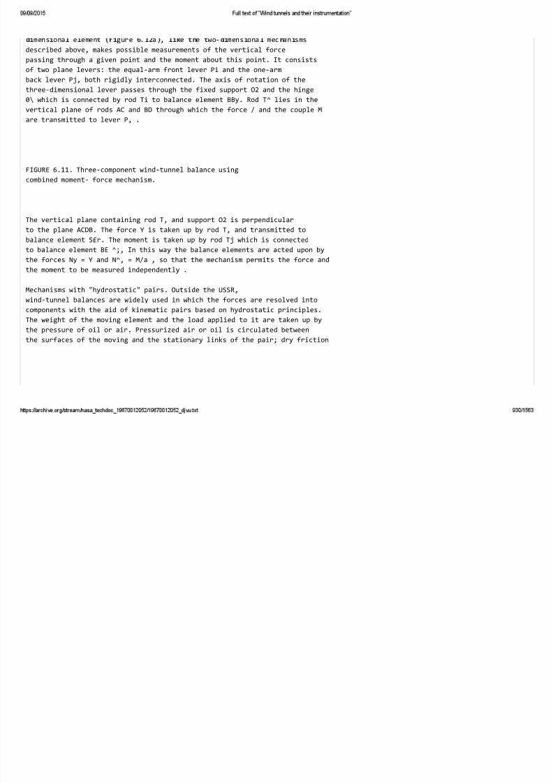
mens ona e emen gure . a , e e wo‐ mens ona mec an sms

described above, makes possible measurements of the vertical force

passing through a given point and the moment about this point. It consists

of two plane levers: the equal‐arm front lever Pi and the one‐arm

back lever Pj, both rigidly interconnected. The axis of rotation of the

three‐dimensional lever passes through the fixed support O2 and the hinge

0\ which is connected by rod Ti to balance element BBy. Rod T^ lies in the

vertical plane of rods AC and BD through which the force / and the couple M

are transmitted to lever P, .

FIGURE 6.11. Three‐component wind‐tunnel balance using

combined moment‐ force mechanism.

The vertical plane containing rod T, and support O2 is perpendicular

to the plane ACDB. The force Y is taken up by rod T, and transmitted to

balance element S£r. The moment is taken up by rod Tj which is connected

to balance element BE ^;, In this way the balance elements are acted upon by

the forces Ny = Y and N^, = M/a , so that the mechanism permits the force and

the moment to be measured independently .

Mechanisms with "hydrostatic" pairs. Outside the USSR,

wind‐tunnel balances are widely used in which the forces are resolved into

components with the aid of kinematic pairs based on hydrostatic principles.

The weight of the moving element and the load applied to it are taken up by

the pressure of oil or air. Pressurized air or oil is circulated between

the surfaces of the moving and the stationary links of the pair; dry friction

 

 

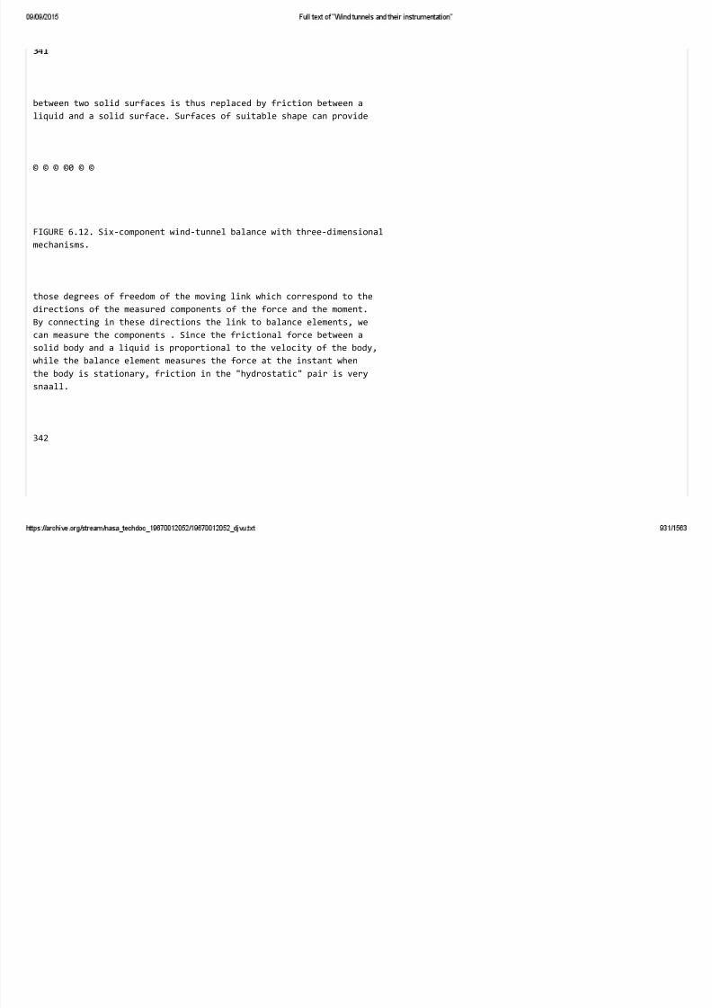
between two solid surfaces is thus replaced by friction between a

liquid and a solid surface. Surfaces of suitable shape can provide

© © © ©0 © ©

FIGURE 6.12. Six‐component wind‐tunnel balance with three‐dimensional

mechanisms.

those degrees of freedom of the moving link which correspond to the

directions of the measured components of the force and the moment.

By connecting in these directions the link to balance elements, we

can measure the components . Since the frictional force between a

solid body and a liquid is proportional to the velocity of the body,

while the balance element measures the force at the instant when

the body is stationary, friction in the "hydrostatic" pair is very

snaall.

342

 

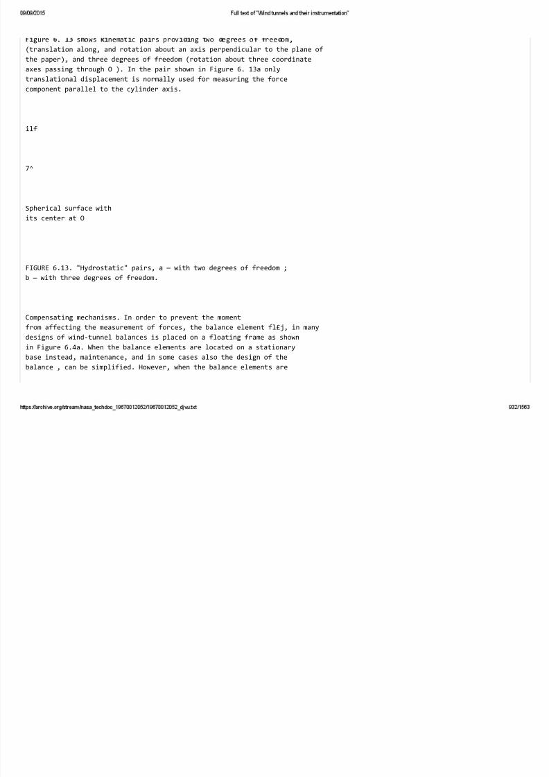
gure . s ows nema c pa rs prov ng wo egrees o ree om,

(translation along, and rotation about an axis perpendicular to the plane of

the paper), and three degrees of freedom (rotation about three coordinate

axes passing through O ). In the pair shown in Figure 6. 13a only

translational displacement is normally used for measuring the force

component parallel to the cylinder axis.

ilf

7^

Spherical surface with

its center at O

FIGURE 6.13. "Hydrostatic" pairs, a — with two degrees of freedom ;

b — with three degrees of freedom.

Compensating mechanisms. In order to prevent the moment

from affecting the measurement of forces, the balance element fl£j, in many

designs of wind‐tunnel balances is placed on a floating frame as shown

in Figure 6.4a. When the balance elements are located on a stationary

base instead, maintenance, and in some cases also the design of the

balance , can be simplified. However, when the balance elements are

 

oca e on groun , ecomes necessary o compensa e e a ona

force acting on the floating frame in the direction of the link rod of the

balance element /?£«

For instance, if in the system shown in Figure 6.4a we transfer the

balance element to "ground", as shown in Figure 6.4b, rod T\, which

connects lever P^ to the balance element BEm^ will also take up part of

the vertical load, unloading rods AC and BD. In order to direct this part

of the load to balance element BEy, a compensating lever P^, having the

same transmission ratio as levers P, and Pj, is provided.

Figure 6. 14 shows a three ‐component wind‐tunnel balance /3/. For

measuring drag and lift, the floating frame F, has two degrees of freedom

in translation, provided respectively by the parallelogram mechanism

ACDB and the adding mechanism consisting of levers P, and Pj. For

measuring the moement Af,, a second floating frame Fj is connected to F,

by a pyramidal support whose instantaneous center of rotation lies on

the ^‐axis. Since the balance element which measures the moment is

343

installed on the "ground", the external forces acting on floating frame f i

consist, in addition to the aerodynamic forces, also of the force MJl in

the horizontal rod EF connecting the "moment" frame F2 to balance

element BE^z ■

FIGURE 6.14. Removing the reaction moment from the balance element BEf^

 

Part 5C' of the horizontal rod 5I>', connecting frame Ft to the system

for measuring the force Q, is acted upon by a load ‐Q + M^jl . The

compensating device used in this system differs from the previous one

(Figure 6, 4b) in that the compensating lever P3 has a fixed fulcrum. An

equal‐arm lever Pj is hinged at the center d of lever P3 . One end of

lever P4 is connected to rod EF , and the other end to balance element BE^^

(through an intermediate crank lever). A force S/MJ/ acts on lever P4 at O, .

The moment due to this force, about the fixed support O2 of lever P3 ,

is balanced by the moment due to the force acting in part BC'of rod BD'.

Thus when only a couple acts on the model, the force in CD' is zero and

balance element BEq does not take up any load.

In wind‐tunnel balances without measuring hinges on the model, where

the naeasured moments are transmitted to the balance elements through a

floating frame, the latter is in addition to the components of the aero‐

dynamic moment, also acted upon by the moments due to the reactions in

the hinges of the links connecting the fram.e with the balance elements.

The effect of the reaction moments on the balance indications can also

be elmininated by comipensating devices.

Thus, for instance, in three ‐component wind‐tunnel balances

(Figure 6. 11) the drag is taken up by the horizontal rod T , connecting the

floating frame to the balance elements through crank lever Ps. Rod T

344

is connected to the floating frame at a distance h from the jc‐axis. Hence,

 

n a on o e momen e rame s a so ac e upon y a coun er‐

clockwise moment due to the couple Qh. The lower hinge of the rod

connecting lever P3 to balance element BEm^ is loaded by the force

A'^ = (VW, ‐QA)

1— /

To balance the moment Q/t, crank lever P5 is connected by a rod to the

fulcrum of a compensating lever P, whose ends are hinged to rods connected

to balance elements BEmz ^"^"^ ^^<3 ■ ^ ^^e arms of lever P5 are equal,

lever Pt transmits to balance element BE^z an additional load

The total load acting on balance element BEm^ is

1 — ; L

NM = NM + i^M = {M, ‐ Qh) ‐

I

 

Thus, when the compensating lever P4 has a transmission ratio

mln={\ — i)Lh/cl , the effect of the drag Q on the measurement of M,

can be eliminated. The loads on the balance elements will then be

N„ = ‐^— ‐J‐ M, ,

N^

(i‐t)Q‐

If the direction of rod T coincides with the ^c‐axis, as shown in

Figure 6. 11 by the broken line, then A = 0, min = , and no compensating

lever is necessary.

FIGURE 6.15. Compensating the reaction moment

by applying to the floating frame an opposing mo‐

ment.

345

 

n e sys em s own n gure . , e n uence o e reac on

moment Qh is eliminated by adding a load to balance element BEmz ■ A.n

alternative naethod is to apply to the floating frame a moment opposed to

the reaction moment (Figure 6. 15), The floating frame is suspended

at A and B from a lever system (not shown) which measures the vertical

load and the moment while at /I' and B' it is connected by rods to levers P^

and P3 which have the same arm ratio a/6. Lever P3 takes up part

of the load due to the force Q, which is transmitted by means of

lever Pi, having a transmission ratio m/n, and equal ‐arm crank lever P5 .

This load, equal to Qm/n, causes equal and opposite forces in rods A'C

and S'D' which cause a moment Qm{a + h)Llbn to act on the floating frame.

This moment is opposed to the reaction moment Qh. Hence, if the

transmission ratios of levers P2, P3, and P4 are such that

m (a+b) ^_

n b

the reaction moment will be fully compensated.

Elements of wind‐tunnel balances

The main elements in the described mechanisms of wind‐tunnel balances

are levers, hinges, and rods. Sensitivity and accuracy of the balances

depend on the design of these elements, which are very similar to those

used in ordinary balances. The main design requirements are:

1) small friction during measurement displacements;

2) high sensitivity;

3) high accuracy of the transmission ratios of the levers in the adding

and "moment" systems;

 

4) rigidity of all levers, rods and frames; this is necessary for minimum

distortion of the system under the action of aerodynamic loads;

5) adjustability of the fixed supports, to permit elimination of

systematic errors due to initial incorrect installation of the system.

The first two requirements are best met by lever systems employing

knife edges and elastic hinges. Ball bearings should be avoided, but

are sometimes used in highly loaded supports of crank levers. In this

case the effects of friction are reduced by using large lever arms; this

decreases the work done by friction when the levers undergo angular

displacements.

Knife edges. Figure 6.16 shows two types of knife edges which are

very often used in wind‐tunnel balances. A double knife edge (Figure 6. 16a)

ensures high stability of lever (1) in relation to its longitudinal axis, and

is generally used as fixed or main support of a lever. The second design

(Figure 6.16b) is employed for connecting a lever with a rod. In both types

of hinges, the working edges of the knives are obtained by milling surfaces

forming angles of 50 to 60° in cylindrical rods (2). Pads (3) are self‐

adjustable along pins (4) which are perpendicular to the knife edges.

The other degrees of freedom of the pads, necessary for aligning the

knife edges with the notch in the pad in case of manufacturing errors.

1680

346

 

are prov e y ra a an ransverse c earances e, an e o . o . mm.

To prevent lateral friction between knife edge and pad, the lateral surfaces of

the latter have conical protrusions whose peaks press against the knife

edge, while the end surfaces of the latter are milled at right angles to the

edge (Figure 6.16a). Alternatively the lateral surfaces of the pad are flat

while those of the knife edge are formed by two planes each, whose

intersections are coplanar with the edge and inclined to it at angles of

60 to 75° (Figure 6. 16b).

Lever support

FIGURE 6.16. Knife edges, a — for main support of lever; b — for con‐

necting lever and rod.

In order to prevent the knife edge from sticking between the pads, an

axial clearance es of 0.2 to 0.3 mm is provided. The knife edge is fixed

to the lever with the aid of integral flange (5). This design permits

adjustment of the lever ‐arm. lengths by turning the knife edge about the

axis of its cylindrical part, which is at a distance A from the edge. After

adjustment the knife edge is fixed in the lever with the aid of pin (6).

Figure 6. 17 shows another design of a knife edge used in fixed lever

supports. The triangular knife edge (1), which is pressed into lever (2),

is supported on a split pad consisting of two parts (3) and (4), inter‐

connected by rings (5) located on projections of said parts. The opening

between parts (3) and (4) contains, perpendicular to the knife edge.

 

347

a roller (6) on which pad (3) can turn. Rotation of the pad about an axis,

perpendicular to the axis of knife edge (1) and roller (6), is made possible

by the cylindrical tail of part (4) being inserted into a hole in support (7).

Axial displacement of the knife edge beyond the permitted clearance e^ is

prevented by plate (8), fixed by screws to pad (3).

FIGURE 6.17, Knife‐edge support.

The knife edge and pad are made from case‐hardened alloy steels

which are heat‐treated. The pads have a Rockwell hardness of 63 to 65.

FIGURE 6.18. Single‐stage elastic hinges; a — without fixed center;

b, c ~ with fixed center.

348

To prevent the knife edges from leaving marks on the pad surfaces, the

 

ar ness o e ormer s o egrees ess an a o e pa s. e

case‐hardened layer has a thickness of 0.8 to 1mm. Pads and knife edges

can also be made from noncarburized steel and have equal hardness. The

load acting on hardened knife edges is usually 200 to 400 kgs per cm of

edge length.

The drawback of knife edges is that they can take up only positive loads

which force the edge onto the pad. When negative loads have also to be

measured, the balances are preloaded by counterweights. These counter‐

weights are calculated in such a way that at the maximum possible negative

aerodynamic forces the loads on all hinges will still be positive.

Transverse loads on the knife edges are permitted only within small limits

(of the order of a few % of the normal load).

Elastic hinges. Elastic hinges are plates which have low bending

rigidity in one plane but a considerable rigidity in a plane perpendicular

to the first.

The advantages of elastic hinges over knife edges are: 1) simplicity

of manufacture, 2) high reliability in operation and ease of obtaining

hinges with two degrees of freedom, required for three‐dimensional

measurement systems, 3) complete absence of friction, 4) capability

of taking up loads of different signs.

FLGURH 6.19. Two‐siep elastic hinges.

There are two types of elastic hinges: hinges without fixed centers and

hinges with fixed centers. In an elastic hinge without fixed center

(Figure 6. 18a) the position of the instantaneous center of rotation depends

 

on e e orma on o e nge; suc nges are ere ore use or x ng

rods to levers and floating frames only when the displacements of the

latter are very small. Hinges without fixed centers cannot take up

transverse loads.

349

Hinges with fixed centers consist of two or more plates intersecting

at right angles (Figure 6. 18b and c). The hinge shown in Figure 6. 18c

is made by milling side openings into a hollow cylinder. Under the action

of the moment applied to it, the frontal part of the cylinder turns, in

relation to the rear part, by a small angle about the axis of the cylinder.

Hinges with fixed centers are used as principal supports of levers and can

take up considerable transverse loads.

FIGURE 6.20. Lever on elastic hinges.

The design of elastic two‐step hinges is shown in Figure 6. 19. A two‐

step hinge can be made by machining mutually perpendicular planes into

a rod (Figure 6. 19a). In this widely used design the instantaneous axes

FIGURE 6.21. Crank lever on elastic hinges.

 

of rotation in the two planes do not coincide, but this is usually not important.

Rods with such two‐step hinges at both ends are suitable for interconnecting

350

levers with nonparallel axes of rotation, or with parallel axes of rotation

when, due to manufacturing errors, the rods are slightly inclined to the

planes of rotation of the levers.

Figures 6. 20 and 6. 21 show levers on elastic hinges. The principal

hinges, which ensure the required transmission ratios (for instance, in

lever adding systems), are very often knife edges, while elastic hinges

are used for those links of the system which need not have accurate

transmission ratios, since they are adjusted with other links or parts

of the system.

Elastic hinges are milled from high‐alloy steel rolled sections.

Machining is carried out after heat treatment designed to provide a yield

stress of about 80kg/mm^. After this heat treatment steel can still be

machined. In order to avoid stress concentrations, transitions from thin

to thick sections must have fillet radii not smaller than the plate thickness.

The nnaximum permissible load must not exceed 0.3 to 0.4 times the yield

stress. Elastic hinges made from flat spring steel are simpler to

manufacture but less reliable, since it is difficult to fit them without

clearances. Reliable fixing is the main requirement for elastic hinges.

Experimenters sometimes waste much time finding out why the accuracy

in wind‐tunnel balances is reduced, while the only reason is small

 

c earances n some o e connec ons o e e as c nges.

The main characteristic of the elastic hinge is its rigidity or stability.

When the hinge is turned the bending stresses in the material cause a

restoring moment proportional to the angle of rotation. When this angle Is

very small, the restoring moment is much higher than the frictional

moment of an equivalent knife edge. Hence, these hinges are best used

in those elements of lever systems of wind‐tunnel balances, which take up

the highest loads, and thus have the smallest displacements. If necessary,

elastic hinges can be used when the angles of rotation are large (up to

several degrees of an arc); their extreme rigidity is then compensated by

inserting into the system unstable links, for instance, of the type shown in

Figure 6.43.

Hermetically sealed openings for rods. In several designs

of supersonic wind tunnels the floating frame of the balance is inside a

hermetically sealed chamber surrounding the test section, while the lever

system of the balance is outside the chamber. In order to lead out the

force ‐transmitting rods from the chamber, packings are used which prevent

entry of air into the chamber from the atmosphere. A reliable packing,

which frees the rod from the action of the difference of pressure in the

chamber and the surrounding atmosphere, is shown in Figure 6. 22.

Packings are made from multi ‐ribbed metal membranes (bellows) which

have a relatively small rigidity. Similar packings are sometimes used

to lead out parts of the model support from the test section of the wind

tunnel.

Model supports. According to the method of connecting the model

to the balance system we distinguish between flexible supports (wires or

tapes) and rigid supports (stands or struts). Wire supports, first used

by Prandtl in wind‐tunnel balances of his design, are still used in some low‐

speed wind tunnels. Many wind‐tunnel balances with wire supports have no

floating frames, since the wires (or tapes) themselves, when tensioned

by counterweights, can serve as links of the mechanism for resolving

 

e orces n o componen s.

351

The principle of measuring forces, used when the model is flexibly

supported, is illustrated in Figure 6. 23. The vertical force Y is directly

Balance lever

Chamber

FIGURE 6.22. Hermetically sealed rod outlets.

Chamber

taken up by wires (1) and (2), pre ‐tensioned by counterweights G, and G2.

When wires (4) and (5) are inclined at angles of 45°, the tension in wires

(2) and (3), due to the counterweight G2,is Q,Y2l2 . The change in

tension in wire (3), which is measured by balance element BEq, is equal

to the drag Q of the model.

 

^V'^f

GfH^

FIGURE 6.23. Resolving a force into components v/ith the aid of wire

supports.

The three‐strut support (Figure 6. 24) is m.ost widely used for fixing

the model to the floating fram.e of the balance in a subsonic tunnel. The

parts adjacent to the model have the shape of symmetrical airfoils. In

order to reduce the drag of the struts and increase the measurement

accuracy, those parts which are farthest away from the model are covered

with shrouds secured to the wind‐tunnel walls. The shroud of the trailing

352

support, which moves in the flow direction when the angle of attack of

the model is altered, has a large clearance in relation to the strut or is

moved with the aid of a servo mechanism along the tunnel wall in such

a way that the clearance between the support and the shroud remains

constant.

 

^ f ^

FIGURE 6.24. Three‐Strut support devices. 1 — leading strut; 2 — shrouds:

3 — trailing strut; 4 — mechanism for altering angle of attack.

At large flow velocities, interference between the supports and the

model increases, but its influence is difficult to determine. At transonic

velocities the additional blockage of the tunnel by struts and shrouds is

very serious, and may lead to premature choking of the tunnel. Shocks

at the unshrouded parts of the struts cause additional drag whose magnitude

varies considerably even with small changes in flow velocity.

'//////yyj//yy/yyy/y//y//y///yy////yyyy/////////^.

^777777^7y777777777777>7777?ZP77777777777?:^7777i

FIGURE 6.25. Arrow‐type struts.

The degree of tunnel blockage, the additional drag, and the effect of

 

e s ru s on e ow aroun e mo e can e re uce y e use o arrow‐

type struts (Figure 6. 25) or arrow‐type tape supports.

It is also possible to fix models of rockets or airplanes with short wings

on single rigid arrow‐type struts. The angle of attack of the model is in

this case altered with the aid of a rod inside the streamlined strut

(Figure 6. 26).

353

A serious drawback of wind‐tunnel balances with strut supports is

the reduced accuracy of measuring side forces and heeling moments.

Floating frame of balance

FIGURE 6.26. fvlodel fixed to single arrow‐type

strut

A small asymmetry of the supports, a small flow inclination, or non‐

symmetrical shocks cause a transverse force to act on the strut.

 

y y y .

FIGURE 6 27. Cantilever support . 1 — model; 2‐

cantilever support; 3 — strut; 4— shroud.

This force, taken up by the balance element measuring the side force,

also causes a moment about the x ‐axis of the balance, which is taken up

by the balance element measuring the heeling moment M^ on the model.

It is not always possible to eliminate completely the additional loads

taken up by the supports at large flow velocities.

The perturbations caused by the struts at the sides of the nriodel

distort the flow pattern near the model at supersonic velocities in a

way that cannot practically be taken into account. Hence, in a supersonic

wind tunnel the model is installed with the aid of a cantilever tail support

(Figure 6. 27). Downstream, the support is rigidly fixed to a strut

mounted at the rear of the test section, where its presence does not affect

354

FIGURE 6.28. Semicircular strut. 1

model; 2 — cantilever support ; 3

semicircular strut: 4— shroud.

 

the flow in the test‐section where the model is installed. This installation

is particularly suitable for models of naodern rockets and airplanes having

blunt tails. In mechanical wind‐tunnel balances, which are placed outside

the test section, suppo.rts and struts must

be shrouded.

A good system of supports in a super‐

sonic wind tunnel is shown in Figure 6. 28.

Model (1) is fixed at its tail to cylindrical

cantilever support (2), which is installed in

the central part of strut (3). The latter is

shaped like an arc of a circle whose center

is at the origin of coordinates of the

balance . The tail support and the strut

are covered by shroud (4), which turns

together with the strut when the angle of

attack of the model is altered. A servo

device, which synchronizes the rotation

of strut and shroud, permits a constant

small clearance to be maintained between

the strut, which is connected to the

balance , and the shroud, which is

connected to the tunnel walls. This design

permits the cross section of the shroud to

be reduced to a minimum.

The minimum sections of strut and tail

support are determined from their deformations. Under no circumstances

must the deflected support touch the shroud since otherwise part of the

aerodynamic forces would be taken up by the shroud and the balance would

 

g ve a se n ca ons. n or er o ncrease e range o ang es o a ac ,

supports curved in the xy‐plane are sometimes used. Curved supports

serve also in model tests at different slip angles. In this case the plane

of bending is perpendicular to the plane in which the angle of attack

changes.

Figure 6. 29 represents a simplified diagram of the balance for the

18"X20" cross‐section supersonic wind tunnel of the Jet‐Propulsion

Laboratory of the California Institute of Technology. The floating "moment"

frame of the balance , to which an arc ‐shaped strut is fixed, rests on a

pyramidal rod system. The instantaneous axis of rotation of the floating

frame coincides with the axis of the strut, about which the latter can turn

on the floating frame, and with the z ‐axis of the balance /7/.

For load tests of airfoils in supersonic wind tunnels the model is

inserted with a small clearance through the tunnel walls which can be

rotated in order to maintain the clearance constant at different angles of

attack. When optical observations of the flow around the model are under‐

taken simultaneously with the force measurements, the rotating walls are

made from , optical glass (Figure 6.30). Such designs are used also for

measuring forces acting on half‐models, i. e., three‐dimensional models

of wings or finned bodies which are installed on the tunnel wall in such

a way that the plane of synimetry of the model coincides with the plane

of the wall (Figure 6. 31).

355

FIGURE 6,29. Six‐component wind‐tunnel balance

with curved strut, of the California Institute of Technology.

 

 — suppor ; —momen a e; — a ance; —

force table; 5 —balance element ; D — drag; S —

side force; P — pitching moment; R — heeling moment;

Y —yawing moment; L — lift; 6 —struts of pyramidal

floating‐frame suspension; 7— shroud; 8 — wind

tunnel.

Airfoil

'/>/////////////,

To mechanism for

adjustment of angle

of attack

Slot

Protective glasses

rotated together

with model

 

FIGURE 6.30. Airfoil mounted in a supersonic wind tunnel.

356

•,,11111111, l>>lll>\)ll >l>lIlt>>irTTT.

■Balance

FIGURE 6.31. Half‐model mounted in

a supersonic wind tunnel.

§26. DESIGN EXAMPLES OF WIND‐TUNNEL

BALANCES

Wind ‐tunn el balances for low‐speed tunnels. Figure 6. 33

is a simplified diagram of a six‐component wind‐tunnel balance with a

s,(e;)tl t\B^(e;)

 

FIGURE 6.32. Six‐component wind‐tunnel balance i^ih flex‐

ible model suppofts.

357

flexible tape suspension. ._ Balances of this type are intended for tunnels

■with open test sections, as are installed in the subsonic tunnel of the

Moscow State University, The balance is mounted on a platform

supported by columns on a carriage located outside the flow. The

carriage with the balance and the suspended model (Figure 6. 33) is rolled

onto a rotating table in the test‐section floor; by turning this table about

a vertical axis/ the angle of yaw g of the naodel can be altered.

FIGURE 6.33. Carriage with wind‐tunnel balance (see diagram in Figure 6.32).

The tested model is suspended from the balance at points A, B and C

(Figure 6. 32) in inverted position by m.eans of a combined suspension which

consists partly of rigid shrouded rods and partly of tapes of streamlined

section. Th e origin of coordinates of the m.easuring system is at the mid‐

point of ^ S in the vertical, plane, of symmetry of the model. The same

plane contains the tail support point C of the model. At A andB , two

horizontal rods are secured ‐wrhich are connected at D and E to inclined

 

ens on w res, xe a an , an o ver ca apes connec e o e

horizontal beam Ti. Counterweights Gi, gI, Gs, G2 and G3 serve to pre‐

tension all tapes, as shown at the bottom of Figure 6.32. The tensions

in rods AD and BE , caused by the aerodynamic forces acting on the model,

are respectively ‐^‐\ i and— i. where / is the distance between ^4

and B.

Since the inclined tension wires form angles of 135° with the horizontals

and verticals, the total vertical force acting on beam 7"i is equal to the sxsxd.

of the forces acting on rods AD and BE . The drag Q is measured by balance

element SEq with the aid of levers Pi, Pj , and P3. The moment, due to the

358

vertical forces acting on beam 7"i, is equal to the moment /W„ measured

by balance element BE^y with the aid of lever P, . The lift is taken up

by tapes Li, L2, L3 and I,; the directions of tapes Li, L2 and ia lie in the

same vertical plane. Beam Ti takes up that part of the lift which acts

at A. Since tapes L, and 1,2 are inclined to the vertical, beam Ts takes up

also the total side force Z.

In order to transmit these forces to the balance elements BEy and BE, ,

beam Tj is suspended from rocking lever B| . This permits translational

motion of beam Tj in the yz plane. Rocking lever B\ takes up all moments

acting in the vertical plane on beam T2 and prevents its rotation. Tape I‐3

is fixed to beam Ts which is suspended from rocking lever Bj similarly as

beam T^ is suspended from rocking lever Bj.

 

y rearrang ng e po n s a w c e apes are xe o eams an

Ta, we can vary the length / without affecting the equilibrium conditions of

the system. Beams T^ and T3 are connected by rods to levers Ps, Ps and P^

intended for measuring the lift Y and the heeling moment Mx. The vertical

force acting on tape L^ is proportional to the pitching moment Mz. At C

this tape is fixed to a rotating lever of the mechanism for altering the angle

of attack (column K). The length L can be varied by fixing hinge C to

different holes in the lever. The mechanism for altering the angle of attack

is suspended from, lever P9, one end of which is connected to balance element

BEm, . The other end is connected to lever P,„ of the system for measuring

the lift Y.

The load transmitted to lever Pg is equal to the vertical force in tape

CC, since five horizontal rods, connecting column K to fixed points, prevent

its movement except for vertical translation. Heeling mom.ents are

measured with the aid of lever P7 which is connected by a rod to balance

element BEmx ■ The side force Z is taken up by beam T2 and transmitted to

balance element BE, with the aid of crank lever P,, and intermediate

lever P,2 .

The loads on the balance elements are

NQ = {Q+02 + Q'2)ix.

^M~

M,

 

  + ,‐ , ,, ,

NM‐{''^+02‐02)iMy.

^M=[

where (i,, . . . , im^) are the transmission ratios of the lever systems and a

is the angle of attack of the model.

Knowing the calibration coefficients (A^, . . ., kM^) the components of the

aerodynai^ic forces acting on the model are

Q=kj, (rix ‐nx.)—Qs, Mx = k^, [n„^ ‐ «^_^ j — M^^ ,

359

aerodynamic forces due to the supports, which are determined by operating

the tunnel without the model, while n with the corresponding subscript is

the indication of the balance element. The additional subscript

corresponds to the zero readings of the balance elements before the

experiment, when no aerodynamic forces act on the model.

 

The counterweights are selected not only for tightening the suspension

system but also for pre ‐tensioning certain balance elements to enable

them to measure negative loads . For this the following inequalities must

hold:

0.‐|‐0; + G3>l‐K,„!,

(0,‐0;)/>i‐yW,,„|,

03^C0S£t>|‐/M,„„|.

An example of a balance with rigid supports is the six‐component wind‐

tunnel balance of the University of Washington (Figure 6.34). This balance.

FIGURE 6.34. Six‐component wind‐tunnel balance of the University of Washington.

I — movable strut; 2 — fixed strut; 3 — motor‐driven lead screw for moving strut;

4 — shroud: 5 — motor for adjusting angle of attack a ; 6 — motor for adjusting

angle of yaw p ; 7 — rod for transmission of force; 8 — crank lever to take up drag;

9 — rods to take up lift; 10 — rods to take up reaction due to heeling moment;

II — crank lever to take up pitching moment; 12 — pedestal; 13 — electromagnetic

balance element.

360

 

n en e or measur ng orces n a ow‐spee unne av ng a c ose

test section measuring 3.6mX2.4m, has electromagnetic balance elements

and vertically disposed links of the lever system. The basic lever

system consists of tubes A,

B, C and E supported on universal elastic hinges.

The inner tube A contains the support for the

model and transmits the aerodynamic forces

acting on the latter to the outer tubes (levers)

B and E.

The outer tube C is a compensating lever

which permits independent measurement of Q

and M,, or Z and Mx, as illustrated in

Figure 6.34a which shows the connections of

the levers for measuring the components Q and

Mj. Similar connections of levers in the plane

passing through the vertical axis and

perpendicular to the plane of the paper, enable

Z and M,. to be measured. For independent

measuring of all four elements it is necessary

that the following relationships obtain between

the transmission ratios of the levers:

', 1 +

 

■)+^‐

The magnitudes entering into the above

formulas are indicated in Figure 6. 34a.

When these conditions are satisfied, the forces

in the rods connecting the levers with the

balance elements BEq and BEm, are respectively

FIGURE 6.35, Six‐component wind‐

tunnel balance on hydrostatic pairs. 1 —

support (dynamometer for measuringY);

2— main floating frame; 3— flat pad; 4 —

intermediate floating frame; 5— spherical

pad; 6— moment frame; 7 — dynamometer

for measuring M^; 8— rod; 9— dynamo‐

meters formeasuring ^^and m ; 10— jY = (/,‐[‐/) ‐—^ .

dynamometers for measuring z; 11 —

dynamometer for measuring g; 12‐rod. ^^^ ^^^^ conditions are necessary for the

independent measurement of Z and M». The lift is transmitted to the balance

element BEyV/ith the aid of rod (9).

Figure 6.34b shows the system for measuring My. The main lever /I is

connected by hinges through rods S, to floating lever P, . Rod Sj, which is

perpendicular to S, , connects the lever to the fixed hinge O. A couple thus

counteracts the moment My. One constituent force acts along rod S2 and

the other along rod 53 which is connected to balance element BEm^.

 

The model support consists of fixed strut (2), mounted on tube A, and

movable strut (1), which serves for altering the angle of attack by means of

a motor ‐driven lead screw. For changing the angle of yaw, the entire

support can be turned by another motor /26/.

Wind tunnel balances with hydrostatic pairs. Balances

with hydrostatic pairs are used mainly in large transonic wind tunnels where

the aerodynamic forces acting on the model amount to hundreds or thousands

of kilograms.

The designs of the six‐component balances for the wind tunnels in Modane

(France) and Pasadena (U.S.A.) are based on the same principle (Figure 6.35).

361

The main floating frame (2) rests on three supports (dynamometers) (1).

Three hydraulic dynamometers are inserted between the supports and

the fram.e in order to measure the lift. Three flat pads (3), resting on the

upper surface of the main frame, carry an intermediate floating frame (4).

The surfaces of the pads and the support plates of frame (4) are polished.

During measurennents oil (or air) is constantly circulated between the pads

and the internnediate frame, which is supported on a layer of liquid and can

slide over pads (3) with negligible friction. The intermediate frame is

restrained in the longitudal direction by rod (12) which connects the frame

to dynamometer (1 1 ) which is fixed to the main frame and takes up the drag

Q of the model. Frame (4) is restrained in the transverse direction by two

horizontal rods connecting it to frame (2) via two dynamometers (10). The

sum of the loads on these dynamometers is equal to the side force Z.

 

e upper par o e n erme a e rame carr es ree pa s w

spherical surfaces whose center lies on the wind‐tunnel axis and is the

origin of the balance coordinate system. The spherical pads carry on oil

films the m.oment frame (6), which takes up all moments and forces acting

on the model. The forces are transnaitted through the intermediate frame

to dynamonaeters (1), (10), and (11).

The moments tend to rotate frame (6) which can slide with negligible

friction on pads (5). Rotation of the frame in the vertical plane passing

through the tunnel axis is prevented by rod (8) which connects the monaent

frame to frame (4) via the dynamometer (7) which serves to measure

the pitching moment M,. Rotation of the frame in a transverse vertical

plane is prevented by two horizontal rods which connect frames (4) and (6)

via two dynamometers (9). The sum of the forces acting on these

dynamometers is proportional to the heeling moment M^, while their

difference is proportional to the yawing moment My. Adding and subtracting

is done outside of the balance with the aid of hydraulic measuring

instruments (Figure 6.42).

In wind‐tunnel balances of this type the total weight of the floating frame

can reach tens of tons, but the friction in the system is so small that with

this high weight the system for drag mieasurement is sensitive to forces

of a few hundreds of grams.

The model is usually installed in the normal position and positive lift

unloads the dynamometers.

§27. BALANCE ELEMENTS OF WIND‐TUNNEL

BALANCES

The naain characteristics of balance elements are their load capacities,

accuracy, and rapidity of response.

 

The transmission ratios of the levers used for measuring the separate

components of the aerodynamic forces and m.oments are chosen in such a

way that the maximum possible loads on all balance elem.ents are

approximately equal. In very small wind tunnels or in tunnels with very

low gas pressures the aerodynamic forces acting on the model may amount

to tens or single grams. At such small loads the transmission ratios of

the levers are sometimes less than unity. In large wind tunnels, where

362

the forces acting on the model may reach 1 to 20 tons, the transmission

ratios of the levers are very high (100 to 200).

Rapidity of response is very important in high‐power wind tunnels.

Rapid‐action balance elements permit the test program of wind tunnels to

be increased and the obtaining of experimental data to be speeded up.

The loads taken up by the balance elements can be equilibrated by

counterweights, pressure of a liquid or air, elastic forces, electro‐

magnetic or electrostatic forces. Irrespective of the nature of the

equilibrating force, the balance ‐element indications can be either direct

or by compensation, returning a movable link to its null position.

Elements of the compensating type are most widely used in wind‐tunnel

balances because they permit higher measurement accuracy. In addition,

outside energy sources are used in compensating instruments, which can be

easily used for operating remote‐recording devices.

The required accuracy of the balance elements is determined by the

range of measured values. This range can be very wide, since the same

 

a ance may e use or es ng we ‐ s ream ne o es o revo u on,

having small drag and lift, and transport craft having large drag and lift

at large angles of attack. At the same time wind‐tunnel balances must

enable us to determine relatively small advantages of one model over

another.

Experience shows that these requirements are best satisfied by balances

of the mechanical type, which under conditions of static calibration have

limiting errors of between 1/400 and 1/2000 of the maximum load. Highest

accuracy is only required when measuring drag and lift. Since the system

for resolving forces into components introduces by itself an error into the

measurement, mechanical wind‐tunnel balances have balance elements with

limiting errors from 1/500 to 1/5000 of the maximum load.

Balance elements equilibrated by counterweights

Balance elements based on the gravitational principle can be divided

into lever balances and pointer balances. Equilibrium in lever balances

is usually attained by compensation, the magnitude of the counterweight

being changed at constant lever arm, or by moving a counterweight of

constant magnitude (rider) in relation to the fulcrum of the lever. The

measurement is made at the instant when the lever is in equilibrium in a

given position.

Directly‐indicatingpointer balances equilibrate the load with the aid of

one or several pendulums whose displacements are indicated by a pointer

on a scale. The drawback of these balances is the large motion of the link

which takes up the load. In some cases this may alter the attitude of the

model, and this has to be taken into account. In addition, pointer balances

are less accurate than lever balances. The limiting error in the better

designs of pointer balances is about 1/1000 of the maximum load, while good

lever balances can have a limiting error of less than 1/5000. Pointer

 

a ances are or nar y use w en measur ng very arge oa s, or ns ance

in full‐scale wind tunnels where the size of the balance is unimportant. In

order to reduce the displacement of the model, pointer balances sometimes

have compensating devices (Figure 6.36),

363

iirnini ■■■■ Mill Ill iniiinin ■■iiinini^ ■ i i

Lever elements, equilibrated manually byweights or riders, were widely

used in old designs of wind ‐tunnel balances. Simultaneous measurement of all

components on a six‐component balance requires

many operators who communicate by sound or

sight. Flow fluctuations in the tunnel always

cause certain variations in the forces acting on

the model; hence, manual equilibration is

characterized by large subjective errors and

requires much tinne. At the same time, lever

balances belong to the most accurate measuring

instruments. Automatic lever balances were

therefore developed to provide rapid operation

with a high accuracy. In addition, these balance

elements permit transmission of the indications to

remote recording devices in a simple and readily

available form.

 

e au onaa c a ance e emen gure .

consists of a lever (balance beam) (1), supported

by a knife edge on stand (2). The measured

force P is taken up by the knife edge on the left‐

hand arm of the lever. The right‐hand arm has

an accurate lead screw (6), by which counterweight

(7) can be moved. The lead screw is connected to

a reversible servomotor (5). The rotation of the

servomotor is controlled by transducer (10), which

reacts to displacements of the right‐hand end of the

lever. When the load is increased, the right‐hand

lever end moves upwards, transducer (10) switches

in the servomotor, and the lead screw moves

counterweight (7) to the right, restoring the

equilibrium of the lever. At the instant of equilibrium

the signal of the transducer becomes zero and the

servomotor is stopped. When the load is reduced,

the right end of the lever moves downward, the transducer switches in the

servomotor in the reverse direction, and load (7) moves to the left until

equilibrium is attained again.

At a measured load P, the number of revolutions of the lead screw,

required to restore lever equilibrium, is

Pa

"■ = ‐01'

where t is the pitch of the lead screw, G is the weight of the counterweight,

and a is the length of the left‐hand lever arm. The value of n is shown by

decimal counter (9), in which the digit on the extreme right usually

corresponds to one tenth of a revolution of the lead screw.

The measurement accuracy is increased by using a screw with micro‐

 

me r c rea an y a ng up c earances w e a o spr ngs.

Oscillations of the lever are reduced by hydraulic shock absorber (8). The

electric supply to the motor on the lever is through flexible wires coiled

like spirals. Due to the snaall displacements of the points where the wires

are fixed to the panel, installed near the fulcrum of the lever, the influence

FIGURE 6 36. Displacement

compensation in pointer ba‐

lances. 1 — balance base ;

2 — rod; 3 — screw mechanisms

for adjusting rod length a; 4‐

servomotor; 5 — contacts for

automatic swiiching‐in of

servomotor when rod is pulled

down.

364

of the rigidity of the wires on the sensitivity of the lever is usually

negligible.

FIGURE 6,37 Automatic lever‐ balance element with inductive transducer.

1 — lever, 2 — stand; 3 — selsyn ttansmittet: 4— feedback tacho‐generator;

5 — servomotor: 6 — lead screw; 7 — traveling counterweight; 8 — hydrau‐

lic shock absorber, 9 — counter, 10 — inductive transducer; 11 — amplifier;

 

  — coun er; — rece ver se syn: — pr n ng ev ce.

In mocJern wind tunnels where the measurement data are transmitted

to control cabins, selsyn servo systems are often used. Such systems

consist of a selsyn transducer and a selsyn receiver, instruments which

resemble miniature electric motors. The rotor of selsyn transmission (3),

which has a three‐phase winding, is connected to the servomotor shaft of the

balance element, Underthe action of a variable magnetic field, createdbythe

single‐phase a.c. in the stator of the selsyn transmitter, the rotor of the

latter generates an a. c. voltage which is uniquely determined by the

angular position of the rotor in relation to the stator. Under the action of

this voltage, the rotor of selsyn receiver (13) in the control cabin turns

to the same angular position in relation to its stator. The rotor of the

selsyn receiver is connected with counter (12) and printing device (14).

which records the indications of the counters of several balance elements

in numerical form (see Chapter IX).

The displacement transducer forms together with the servonaotor a

closed‐loop automatic ‐control system in which the control parameter is

the angular position of the lever, the controlling member being the lead

screw with the counterweight. There are several designs of transducers.

The most widely used are inductive (transformer) and contact transducers.

The system shown in Figure 6.3 7 employs an inductive transducer

consisting of a moving coil fixed to the end of lever (1), and located between

two excitation coils wound on stationary iron cores /9/, /lO/. The coil is

excited from one phase of a three‐phase supply. Since the coils are wound

in opposite directions, they create opposed magnetic fields, which induce

in the moving coil an a.c. voltage whose amplitude and phase depend on the

position of the moving coil in the air gap between the stationary coils. The

voltage is amplified by amplifier (11), and is fed to the rotor of

 

 

II I I nil llllllllllllllll llllllllllll llllllllllll IIIIIIIIIHIIlllllllllini ■iiiiiii ■■■■iiiHii ■ ■■ nil II

servomotor (5) which is excited by another phase of the a. c. supply.

If the lever is in equilibrium and the moving coil is in a central position

between the stationary coils, the voltage in the moving coil is equal to

zero and the servomotor is at rest. When the equilibrium is disturbed,

the moving coil is brought nearer to one of the stationary coils, and a

voltage is induced. The servom.otor begins to rotate, and the lead screw

moves the counterweight in the direction required for restoring the

equilbrium of the lever.

The automatic mechanism for controlling the servomotor and the

counterweight must follow the changes in load caused by variations in flow

velocity or in the angle of attack of the model. In order to reduce

oscillations of lever and lead screw, the control system is equipped with

flexible feedback consisting of an inductive tacho‐generator mounted on the

servomotor shaft.

In contrast to inductive transducers, which provide continuous speed

regulation of the servomotor from zero to maximum, contact transducers

cause the servomotor to attain instantaneously a finite speed. The

simplest contact transducer consists of a flexible moving contact located

at the end of the lever in a small gap between two stationary contacts,

AAThen the equilibrium is disturbed, the moving contact closes a circuit

with one of the stationary contacts and the servomotor is switched in;

the latter moves a counterweight on the beam so as to restore the

equilibrium.

 

e raw ac o a ance e emen s w con ac rans ucers s e r

tendency to cause free oscillations of the entire automatic balancing

system when the sensitivity is increased. These oscillations are due

to the inertia of lever, servomotor, and rotating parts, and cause the

position of the counterweight on the lever to vary in relation to its static ‐

equilibrium position. If the amplitude of the load variations is less than

the permissible measurement error, these self‐induced oscillations do

not affect the measurements and cause only burning of contacts.

The counterweight displacements during self‐induced oscillations

increase with angular velocity of the servomotor but decrease with

increasing resistance torque acting on the servomotor shaft after breaking

contact. In addition, they depend on the degree of oscillation damping. In

order not to reduce the speed of operation of the balance elements (the

rapidity of equilibrating at a given load) a two‐speed system is used for

controlling the servomotor (Figure 6. 38), which provides for a sharp

reduction of the rotational speed of the servomotor immediately before

the counterweight attains a position corresponding to static equilibrium

of the lever, and powerful braking of the servomotor after it is switched off.

For this purpose the shaft of servomotor (5) and selsyn transmitter (8)

carries an electroraagnetic brake ( 6) , consisting of an iron rotor rotating in the

magnetic field of a d. c. ‐excited stator. When the rotor revolves (eddy)

currents are induced in it. This causes a torque proportional to the

rotational speed to act on the shaft. The lever has, in addition to the system

of "fine" contacts (1) and (2) also a second system of "coarse" contacts

(3) and (4). The gap between moving contact (3) and stationary contact (4)

is slightly larger than the gap between moving contact (1) and stationary

contact (2). The stator of the brake is supplied with current when contacts

(3) and (4) are open. At a small imbalance of the lever, contacts (1) and(2)

366

 

are closed and the servomotor rotates slowly. At a large imbalance,

the flexible plate containing contact (1) is bent and contacts (3) and (4)

are closed. The winding of the brake stator is short‐circuited, and the

servomotor begins to rotate rapidly.

‐'TTTTTTTTTTm

FIGURE 6.38. Automalic balance element with contact transducer. 1—

moving "fine" contact: 2 —stationary "tine" contact, 3 — moving

"coarse" contact; 4 — stationary "coarse" contact: 5 — servomotor:

6 — electromagnetic brake; 7 — limit switches; 8 — selsyn transmitter

Balance elements with contactless transducers can operate under

conditions of vibrations and fluctuations of the measured forces, when

balance elements with contact transducers lose their sensitivity due to

burning of contacts. Automatic balance elements contain limit switches

(7) (Figure 6. 38), which open the circuit of servomotor (5) when the

measured force exceeds predetermined limits.

 

ro+

YP

4~~^

ffl^a^

W

^'

FIGURE 6.39. Automaiic‐ loading mechanism. 1 — lever; 2 — counter‐

weight; 3, 4 — limit switches; 5 — servomotor for loading; 6 —

moving platform; 7 — weights; 8 — change‐over switch; 9— link for

load suspension.

367

 

The accuracy of measuring forces on wind ‐tunnel balances with lever

elements depends greatly on the degree of damping of the lever oscillations

caused by nonsteady loads on the model. Excessive damping causes delayed

opening of the "fine" contacts, especially if the contact plate is not very rigid.

This causes hunting of the counterweight and leads to self‐induced

oscillations. When damping is very weak after the "fine" contacts open,

the kinetic energy of the lever cannot be absorbed, and self‐induced

oscillations can occur at very small inertial overtravel of the counter‐

weight. Hence, the damping should be chosen in such a way that after

contact (1) and one of contacts (2) are opened, the kinetic energy of the

lever is absorbed before it is able to close the opposite contact.

The amplitudes and frequencies of the force pulsations, caused by

oscillations of the tested model and by flow fluctuations, vary with the flow

velocity, the angle of attack of the model, the rigidity of the suspension

device and lever system, etc. Hence the capacity of hydraulic shock

absorbers of automatic balance elements is sometimes varied with the

aid of electric motors during the experiment, or an electromagnetic damper

is used which is switched in only when the "fine" contacts are open; this

reduces the delay in contact breaking.

In order to increase the load capacity of the balance elements, the latter

are equipped with auxiliary naechanisms for automatic addition of weights.

A single weight balances a load corresponding to the full travel of the

counterweight between the limit switches. A simplified diagram of the

mechanism for weight addition is shown in Figure 6. 39. When the load P

on lever (1 ) exceeds a predetermined value, counterweight (2) moves to

the right and closes limit switch (3). Servomotor (5) is switched on and

lowers platform (6) with weight (7) to a predetermined height, after which

the current to the servomotor is cut off by change‐over switch (8), which

interrupts the circuit of limit switch (3). When the platform is lowered

one of weights (7) becomes suspended on link (9). When the load is

reduced below a predetermined value counterweight (2) closes limit

 

sw c ; s causes e p a orm o r se an a e o a we g rom

link (9).

Pneumatic and hydraulic balance elem.ents

Pneumatic and hydraulic balance elements usually consist of two

separate instruments: a primary instrument taking up the load

(dynamometer), and a secondary measuring instrument (manometer). The

manometers are connected with the primary instruments by metal tubes

up to 20 or 30m long. One of the principal advantages of pneunnatic and

hydraulic balance elements is the sinaplicity of their design, which makes

possible remote measurement. The simplest pneumatic measuring device

is shown in Figure 6. 40, The measured force P is transmitted to bell (1),

which is immersed in vessel (2), filled with mercury or some other liquid.

The pressure in the air space under the bell is thus raised; this increase

is transmitted by a tube to U‐tube manometer (3). If we neglect the wall

thickness of the bell, the differences in heights of the columns of liquid

368

in the bell and in the manometer are respectively

p P

ft, = ‐ET and A, = ‐ij ,

where F is the cross section of the bell, fi and fz are the specific gravities

of the liquids in the bell and in the manometer respectively. The errors

 

 

'WM

u

/3

FIGURE 6,40. Pneumatic balance element.

1 — bell: 2 — vessel with mercury; 'J —

manometer

of indications due to variations in the surface tension of mercury when it

becomes oxidized and contaminated, and by the temperature variation of

Ti and 12 . The range of the measured forces is determined by the

permissible height variation of the column of liquid in vessel (2), and by

the permissible travel of the bell, which is relatedtothe displacement of the

model in the wind tunnel.

FIGURE 6.41. Hydraulic dynamometer. 1 — piston, 2 — cylinder; 3 —

diaphragms; 4. 5— plates: 6 — rods taking up measured load; 7 —

baffle plate: B — nozzle; — air chamber; 10 ‐ bellows; 11 — spring

12 — rod with rack; 13 — pointer; 14 — Bourdon tube.

 

369

Figure 6.41 shows a systemof measuring forces with the aid of ahydraulic

dynamometer with a manometric spring device /ll/. In contrast to other

force‐measuring devices, hydraulic dynamometers permit loads of several

tons to be measured without intermediate lever systems of balance elenaents.

Such hydraulic dynamometers are used in U.S. balances, in which the forces

are resolved into components by means of hydrostatic pairs . In balances

of this type the vertical load, which includes the total weight of the floating

frame, is usually taken up by three dynanriometers which carry the frame.

The dynamometer consists of piston (1), inserted with a small clearance

in cylinder (2). The flat ends of the piston carry diaphragnas (3), which

seal the oil spaces in the upper and lower plates (4) and (5). The full travel

of the piston is about 0.05 mm. The lower oil space is connected by a metal

tube to a measuring device, while the upper oil space is under a constant

pressure po ‐

This design permits measurement not only of positive but also of negative

loads acting on the piston through rods (6). The pressure in the oil space

connected with the measuring system depends only on this load and on the

pressure pn . The pressure in the wind tunnel acts on both sides of the piston

and is therefore not transmitted to the measuring device. The dynamometer

is equipped with volumetric temperature compensation whose operating

principle is the same as in the system shown in Figure 6. 44. When the pressure

changes in the lower oil space, the Bourdon tube (14) of the m.easuring

device tends to bend and thus alter the gap between baffle plate (7) and

nozzle (8), through which air is discharged continuously from a throttle

opening in chamber (9). The change in the gap also causes the pressure

to vary in bellows (10), which is connected with the chamber. When this

 

, ,

of spring (11) in such a way that the position of the Bourdon tube remains

fixed at small displacements of the baffle plate. The tension of spring (11)

and thus, of rod (12) and pointer (13) connected to it, is proportional to

the oil pressure and therefore to the force P .

The spring is made of Elinvar which contains 35% nickel and 8%

chromium. The material has a stress ‐strain relationship which is linear

with an accuracy of 0.05%, and its properties vary very little with

temperature . In certain U. S. wind tunnels, where the balances are

equipped with such measuring devices, the angular motion of the

pointer is converted into electrical pulses which are fed to a system for

processing the measurement data.

Preliminary simplified processing of the data, in order to obtain net

values of the force and moment components, is carried out according

to the system shown in Figure 6. 42, which makes possible wind‐tunnel

balances without lever systems for resolving the forces into

components.

Figure 6. 43 shows a hydraulic system which is a combination of an

automatic lever ‐balance element with a certain type of hydraulic lever. Such a

system is advantageous when, due to space limitations or for other reasons,

the balance elements have to be at a certain distance from the wind tunnel.

The prim.ary instrument consists of bellows (1), connected with bellows (2)

by a brass tube of 2 to 4m.m diameter. Bellows and tube are filled with oil

or distilled water. The pressure, caused by the load P, on bellows (1),

370

 

 

m rpT^

f, ij

Ln in

lt;, ^

FIGURE 6.42. Adding and subtracting forces with the aid of a hydraulic force‐

measuring device.

FIGURE 6.43, Hydraulic transmission of forces 1 — bellows to take up load;

2 — bellows connected with balance element. 3 — balance lever; 4 —

 

  —

compensate for rigidity of bellows (2).

371

is transmitted through the tube to the bottom of bellows (2) which is

connected with lever (3) of the automatic balance element. The left‐hand

arm of the lever is thus acted upon by a force Pj which is equilibrated by

a counterweight.

The displacement of the bottom of bellows (2) depends on the distance

between the contacts of the automatic balance element and usually does

not exceed a few hundredths or even thousandths of a millimeter; when

the system is properly filled with liquid the displacement of the bottom of

bellows (1) is also very small. Hence, hysteresis effects on the bellows

do not influence the measurement of the force P, . The transmission ratio

of the hydraulic system is determined by calibration. It can be assumed

that P2/P1 = FilFi where f 1 and fz are respectively the effective areas of

bellows (1) and (2). When air bubbles are present in the system, the

initial part of the dependence curve can be nonlinear; to avoid this, the

system is filled under vacuum after all connections have been soldered,

or the bellows are preloaded.

^ D‐

 

_2

„ s

^TT‐

FIGURE 6 44. Volumetric temperature compensation for a hydraulic S)stem

1 — bellows to take up load; 2 — bellows connected to balance element: 3 ‐

compensating bellows, 4 — lead screw and reduction gear. 5 — servomotor.

6 — contact connected to movable part of bellows; 7 — stationary contact

In such closed hydraulic systems a change in the temperature of the

surroundings causes a change in the i^olume of the liquid and can be the

cause of systematic errors. If bellows (2) is connected with a null

instrument (as in the case considered), the difference Avi between the

thermal dilatations of the liquid and of the bellows material causes a

displacement 5; = Avt/F, This gives rise to an elastic restoring force

AP( = ciit acting on the bottom and opposing its motion. Here c^ is the

spring rate of bellows (1) and the links connected to it. The magnitude A/'i

is a systematic error of measuring the force P, and is very difficult to

take into account.

 

 

The temperature error AP| can be avoided by means of force or volumetric

compensation. Force compensation consists of applying to the bottom of

bellows (1) a force which is equal and opposite to the elastic restoring

force hPt. Figure 6.43 shows a force‐compensation system which consists

of crank lever (4), whose horizontal arm is hinged at A to bellows (1) and

whose vertical arm carries a weight Q, When the bottom of bellows (1)

moves a distance 8, , the force acting on it changes by

.P,= (.‐^)B,.

Full compensation ( APj = ) is obtained when Qih ~ cia\ ; this is

easily achieved by adjusting the value of U .

In order to compensate fully the reduction in sensitivity caused by lever

(3) being connected to bellows (2), it is sufficient to raise the center of

gravity of the lever by fixing to it a weight Q^ at a height 4 above the fulcrum

of the lever. Similarly to the above, full compensation of the elastic

restoring force acting on bellows (2) is obtained when Q2Z2 = C2a\ . When

02 is large, the weight Q2 becomes heavy; in this case, in its place, the

right‐hand end of the lever is connected to an additional crank lever (5),

shown by broken lines in Figure 6.43, carrying a weight Q'^. For full

compensation of the rigidity of the bellows, the static moment of this

weight about Oj must be

 

 

cia^i.

The ratio a'Jb2 is taken as 1/10 to 1/20, so that Q'^ is some hundreds of

times less than Qj.

I 1= 1 — I ; ^ nt I ^ mirror" • ^'^ Transparent

' [ ' i I I _ ^/4?i screen

Pendulum

FIGURE 6.45. Through‐flow dynamometer. 1— vessel; 2— pressure

regulator: 3 — throttle: 4 — disc: 5 — filter: 6 — pump.

Volum.etric compensation for a closed hydraulic system is illustrated in

Figure 6. 44. The system includes an additional compensating bellows (3),

whose volume can be changed with the aid of lead screw (4), turned by

servomotor (5).

 

373

There is no necessity for teinperat\are compensation in through‐flow

hydraulic dynamometers. Such asystem is shown in Figure 6.45. Oilisforced

by pump (6) into a cylindrical vessel (1), open at the top, after passing through

pressure regulator (2) and throttle (3). On the vessel there is adisc (4), which

takes up the force P whigh has to be determined. Under the action of the oil

pressure, an annular slot is formed between vessel (1 ) and disc (4), through

which the oil is continuously discharged into adrain. The disc thus floats on an

oil film. After being cleaned in filter (5), the oil is returned to pump (6).

When the disc floats up the force P is fully equilibrated by the force of the

oil pressure on the disc. The oil pressure in vessel (1), which is

proportional to the force P, can be measured by any type of manometer.

FIGURE 6,46. Operating principle of wind‐runnel balances resting

on through‐flow dynamometers. 1, 2, 11— through‐flow dy‐

namometers. 3, 4, 5, 6, 7 — piston ‐type manometers; 8 —

adding lever for measuring K; 9 — subtracting lever for measuring

M ; 10 — lever for measuring q .

Figure 6. 45 shows a system for measuring the pressure by a pendulum

piston‐type manometer with optical read ‐out. In order to reduce friction

between the piston and the cylinder the latter is kept vibrating continuously

by the action of an electromagnet.

 

n en e or measur ng orces perpen cu ar o e sc sur ace, e

through‐flow dynamometer permits free motion of the disc in its plane

at negligible friction, the disc floating on an oil film. These characteristics

of through‐flow dynamometers are used for measuring mutually perpendicular

forces. This is illustrated in Figure 6. 46 which is a simplified layout of a

wind‐tunnel balance. The floating frame A of the balance rests on two

through‐flow dynamometers (1) and (2), having equal effective areas.

Dynamometer (1) is connected by tubes to manometers (4) and (6), and

dynamometer (2) to manometers (3) and (5). The pistons of manometers (3)

and (4) are connected by rods to lever (8), which adds the forces acting

374

on these pistons; the indication of balance elements BEy , which is connected

to lever (8), is thus proportional to the vertical force Y . The pistons of

manometers (5) and (6) are connected to equal‐ arm lever (9), which serves

for measuring, by means of balance element BEm, the moment about point O

which is centrally located between dynamometers (1) and (2). Dynamometer

(11) takes up the horizontal component of the force, which is measured with

the aid of balance element BEq, connected by lever (10) to the piston of

manometer (7), on which the pressure in dynamometer (11) acts.

Spring and strain‐ gage balance elements

The accuracy of a spring balance element is mainly determined by the

accuracy of measuring the deformation of an elastic link and the physical

characteristics of its material. The error in measuring the deformations

can be easily reduced to a negligible value if we use an elastic link with a

 

arge a so u e e orma on, or ns ance, a sp ra spr ng.

Servomotor

Counter

FIGURE 6.47 Spring balance element.

Due to hysteresis effects and residual stresses, the error in measuring

forces with the aid of elastic links made from different types of steel is

about 0.2 to 0.5% of the maximum measured force. Better physical

properties are provided by special alloys like beryllium bronze and Elinvar

whose stress — strain relationships are linear with an accuracy of 0.02

to 0.05%.

When spiral springs are used, the effect of their deformation on the

attitude of the model in the test section is eliminated with the aid of a null

method of measurement. The spring is deformed manually or automatically

(Figure 6. 47) so that the lever, which takes up the load from the wind‐tunnel

balance, maintains its initial position. A visual indicator is read off when

the lever is in equilibrium.

Elastic force links in the form of beams subjected to bending have

usually such small deformations that the displacements of the model caused

by them can be ignored. Small deformations are measured with the aid of

different types of electric transducers which convert the magnitude of the

 

375

deformation into a change of inductance, capacitance, or resistance, which

is then measured by an appropriate electrical instrument.

Wide use is made of methods for measuring deformations of elastic

elements with the aid of glued resistance strain gages, which are

described in detail in the next section. A dynamometer with glued

wire transducers is shown in Figure 6. 64. Due to their small dimensions

in comparison with other types of balance elements, such dynamometers

are used in electric strain‐gage balances located inside the model.

FIGURE 6.48, Four‐componeni balance for testing wings. 1 — spindle; 2 —

spindle support: 3 — intermediate frame; 4, 6, 8 — elastic beams with strain‐

gage transducers; 5 — stationary support; 7 ‐ moment lever.

In balances located outside the test sections, strain‐gage transducers

are used very often for measuring aerodynamic loads on half‐models, i. e.

models whose plane of symmetry coincides with the test‐section wall.

Figure 6. 48 shows a four ‐component balance for testing models of wings

1 12/ . A wing model is mounted on spindle (1), by m.eans of which it can

be turned and the angle of attack altered. Spindle support (2) is carried

by a parallelogram, suspension on intermediate frame (3).

The lift Y is taken up by elastic beam (4), which connects spindle

support (2) with franae (3), and is measured by transducers glued to the

beam. Intermediate frame (3) is supported with the aid of beam (6)

on stationary support (5) which permits movement of support (2) and

 

rame para e o e ow rec on. rans ucers, w c measure e

drag Q, are glued to beam (6). The pitching mom.ent is measured with the

aid of lever (7), rigidly connected to the shaft, and beam (8) to which

transducers for measuring AIj are glued. The heeling moment Mj is

measured by transducers glued to spindle (1) where its cross section

is reduced.

The balance shown in Figure 6. 49 employs a support consisting of

curved strut (1) surrounded by shroud (2). The measuring elements A, B,

and C, which have the form of elastic parallelograms, are installed in

such a way that element A takes up only the lift K| while the loads on

elements B and C depend on the drag Q, and the pitching moment jVf,j .

376

The connections of the strain‐gage transducers, which are glued to elastic

elements B and C and arranged in bridge systems as shown at the bottom of the

drawing, permit Q, and /Mj, to be measured independently. The stationary

parts of the elastic parallelograms are fixed to the shroud. In order to

alter the angle of attack of the model, the shroud is turned about the

origin of coordinates O of the balance together with the strut, the elastic

elements, and the model.

Hermetically sealed

chamber

Test‐section

 

wa

FIGURE 6.49 Three‐componenl strain‐gage balance. 1 —

curved strut; 2 — shroud. A, B, C, — strain gages.

Mechanical wind‐tunnel balances may also be provided with balance

elements with nonglued wire resistance transducers. The characteristics

of these transducers are more constant in time than those of glued

transducers whose accuracy is affected by the nonstable properties of the

glue. In the balance element shown schematically in Figure 6. 50, thin

constantan wires are connected to an insulated plate at the end of a lever

mounted on an elastic support, and to two other insulated plates fixed to the

base of the balance element.

The tension in the wires is changed under the influence of the load to

be measured. The change in resistance thus caused is measured by a

Wheatstone bridge, in all four arms of which the wires are inserted.

377

The instrumentation used for this is described in the next section.

FIGURE 6.50. Balance element wiih

nonglued wire resistance transducers.

 

Electromagnetic balance elements

Figure 6. 51 shows two circuit diagrams of balance elements, based on

the interaction between the field of a permanent magnet and the field of ad. c‐

excited coil. Coil (4) is connected to the arm of lever (1), whose other arm.

is acted upon by the force P. The force F of the interaction between

permanent magnet (5) and coil (4) is

F=2KrInH,

where r is the mean radius of the coil, n is the number of turns, H is the

field strength of the permanent magnet, / is the current intensity in the

coil.

When the equilibrium of the lever is disturbed, lever‐motion transducer

(2) sends a signal to amplifier (3). In the circuit shown in Figure 6. 51a,

the lever is returned to equilibrium with the aid of servomotor (7), which

moves the slider of variable rheostat (6). This changes the current

intensity in the coil. The force P is determined from, the current intensity

which is read off from milliammeter (8), or from the position of the slider

of the variable rheostat (at a stable supply voltage), when the lever is

in equilibrium.

The circuit shown in Figure 6. 51b permits faster operation than that

shown in Figure 6. 51a, and can serve for measuring loads changing at

frequencies up to 10 to 20 cycles /13/, /15/. The electric signal from

transducer (2) (photoelectric element, capacitive or inductive transducer)

is am.plified by amplifier (3) feeding coil (4), The current intensity is

measured either directly or by the voltage drop across resistance R. In

this circuit the magnetic system, which consists of coil (4) and magnet (5),

is similar to a spring, since the force F is proportional to the displacement

 

1680

378

of lever (1). The amplification coefficient of amplifier (3) can be so

chosen that at the maximum load the coil moves less than 0.01 mm.

Hence, the rigidity of the electrical spring, on which the operating

speed of the system depends, can be very high. Thus, for instance,

the electromagnetic wind‐tunnel balance element of the University of

Washington has a spring rate of about 2000 kg/ cm and a natural frequency

/

^‐iV —

 

■HLJz:^

V .

h

,1T^5

1

+

1

F

‐©

7

 

FIGURE 6 61. Electromagneiic balance elements.

a ~ equilibration by means of servomotor; b —

static equilibration; 1 — lever; 2 — lever‐ motion

transducer; 3 — amplifier, 4 ‐ coil; 5 — perma‐

nent magnet, 6 rtieostat; 7 — servomotor; 8 —

millianimeier

of 200 cycles /14/. The maximum current in the coil of such a balance

element is between 30 and 50 ma at a maximum load of 3 to 5 kg. Using

an appropriate circuit, an accuracy and linearity of the order of 0.1% can

be obtained. Balance elements of this type can be used in special wind‐

tunnel balances serving, for instance, for measuring loads acting on

vibrating wings.

§28. WIND‐TUNNEL BALANCES

LOCATED INSIDE THE MODEL

As was already stated in the introduction to this chapter, wind‐tunnel

balances located inside the models were developed due to the need to

exclude forces acting on the supports. At supersonic velocities, flow

around the model is least affected by supports in the form of cantilever

379

 

suppor s, n erna w n ‐ unne a ances are ns a e a e o n s

between the models and such supports or in the supports themselves

(Figure 6. 52).

Cantilever support

Shroud

FIGURE 6.62. Installation of strain‐gage balances,

inside model; b — inside support.

When the balance is installed inside the model, the forces acting on the

support are not measured and the support only causes certain perturbations

in the flow at the tail of the model. When the balance is installed in the

support, the latter is protected from the flow by a cylindrical or conical

shroud. The "ground" pressure acting on the rear of the model is

measured with the aid of orifices through which the region behind the model

is connected to a naanometer.

The possibility of installing the wind‐tunnel balance inside the model is

so attractive, that in recent years balances of this type, called strain‐gage

balances, have found very wide use in spite of the fact that their accuracy

and the reproducibility of their indications are still less than those of

ordinary mechanical balances. A measuring error of the separate

components, equal to ±1% (under conditions of static calibration), is

 

  ,

conditions errors of about 0.1%. The latter are very reliable instrunnents

which maintain constant their characteristics for months. Internal

balances have to be calibrated and checked very often, sometimes before

and after each experiment. Particular care should be taken to eliminate

or take into account temperature errors.

A strain ‐gage balance forms an elastic system the deformations of

whose elements are proportional to the components or the algebraic sums

of the components of the total aerodynamic force and moment acting on the

model. These deformations are measured as electrical raagnitudes with

the aid of electrical converters. Wind‐tunnel balances employ almost

exclusively strain‐gage resistance transducers which are based on the

conversion of the deformation of an elastic element into a change of the

electrical resistance, which can be measured by a instrument connected

to a corresponding measuring circuit.

380

strain‐gage resistance transducers

Strain‐gage resistance transducers may be of different designs. Wire

and foil strain‐gage transducers are most widely used. Wind‐tunnel

balances have mostly wire strain‐gage transducers (Figure 6.53) which consist

Base (film or paper)

 

. Base length I

FIGURE 6.53, Wirestrain‐gage‐transducer

of several turns (grids) of wire of very small diameter (0.025 to 0.03 mm),

made from an alloy having a high electrical resistance, and glued between

two layers of paper or film. If the strain‐gage transducer is glued to the

surface of an elastic element, the transducer is deformed together with

this surface. The length / of the wire grid is called the base length of the

transducer. The characteristics of strain‐gage transducers are described

in detail in /1 6/, /17/.

The advantages of strain‐gage transducers, which make them particularly

suitable for measuring aerodynamic forces, are:

1) small dimensions and weight;

2) possibility of measuring very small relative deformations of elastic

elements (less than 10" ); this permits the use of very rigid elastic

elements having high natural frequencies;

3) small inertia, which permits not only static but also dynamic loads

to be measured;

4) possibility of remote measurements.

The main characteristic of resistance strain‐gage transducers is the

coefficient of strain sensitivity, which is determined as the ratio of the

relative change in electrical resistance of the wire to its relative linear

deformation

 

'— iri~r'

where R is the [initial] resistance of the wire, and I is its length.

Thus, if we determine the value of ARIR, we can, knowing the coefficient

of strain sensitivity, find the relative elongation of the wire and, therefore,

of the elastic element to which the strain‐gage transducer is glued:

4£ _ J_ &R_

381

For a monoaxial state of stress, the relationship between the strain e

and the stress a is, within the proportionality limits of the material,

given bye = cjE, where E is the modulus of elasticity of the nnaterial.

The stress at any point of an elastic element depends on the forces

and m.oments acting on this element. Hence, the relative change in the

resistance of the transducer, mounted on the elastic element, is

proportional to the components of the resultant force and moment,

causing the deformation of the element. The coefficient of proportionality

depends on the strain sensitivity of the transduer wire, on the elastic

characteristics of the material, and on the shape and size of the elastic

 

e emen .

In the general case, the state of stress on the surface of an elastic

element, to which a strain gage is glued, can vary from point to point.

Hence, the change in the resistance of the transducer is proportional

to a certain mean stress over the base of the transducer. In order that

the transducer measure the stress at a point (this is particularly important

due to the small dimensions of the elastic elements used in multi‐

component balances located inside models), its dimensions have to be

small. Wind‐tunnel balances employ transducers having bases of 5

to 20 mm and resistances of 100 to 200 ohm. It is possible to obtain

transducers having even smaller bases (down to 2 mm), but a small base

causes the resistance of the strain‐gage transducer to decrease; this

complicates the measurements.

The most commonly used material for wire transducers is constantan,

whose coefficient of strain sensitivity is 5 = 1.9 to 2.1. For approximative

calculations we assume s = 2.

Bridge measuring circuits. The resistance of a strain‐gage

transducer mounted on an elastic element changes very little when the

latter is deformed. Thus, at 0.1% strain

(which, for steel, corresponds to a stress

of about 2000 kg/ cm^), and at an [initial]

transducer resistance of 100 ohm, the change

in the resistance is

^R = Rst = \m■2■ 10"^ = 0.2 ohm

If the measuring accuracy required

corresponds to 0.1% of the maximum stress

(i.e., 2.0kg/cm^), the resistance must be

measured with an accuracy of 0.0002 ohm,

 

 

2X10"^. Such an accuracy can be obtained

only with a compensation method of

measurement, for instance, by means of a Wheatstone bridge.

The simplest measuring bridge consists of four ohmic resistances

(arms) ^1, R2, R3 , and Ri (Figure 6. 54). Points A and B (the supply diagonal)

are at a voltage difference a (from ana.c. ord.c. source), while points C

and D (naeasuring diagonal) are connected to the naeasuring instrument.

Inordinary systems, the strain‐gage transducers are usually inserted

into one or two arms of the bridge, while the other arms are formed by

constant resistances. In wind‐tunnel balances, however, the strain‐gage

FIGURE 6.54. Measuring bridge.

382

transducers are inserted into all four arms of the bridge; this increases

the sensitivity and exploits the bridge characteristics to compensate the

different errors.

If the ratios of the resistances of adjacentbridge arms are equal, i. e.,

/?. ^ ‐ff,

then the potential difference across the measuring diagonal is zero. The

bridge is then balanced.

 

When the resistance of one arm of an initially balanced bridge changes,

a potential difference Au appears between points C and D of the measuring

diagonal. This is the imbalance voltage of the bridge. At small relative

resistance changes the imbalance voltage depends linearly on the sum or

difference of these changes.

The imbalance voltage A" across the measuring diagonal is measured

by an indicating or recording instrument (millivoltmeter or oscillograph

galvanom.eter). Recording instruments of the oscillograph type permit

dynamic processes to be investigated.

In order to obtain high accuracy, A« is measured by a compensating

method with the aid of a separate compensator. In this case the measuring

instrument (zero indicator) serves only as an imbalance indicator for the

compensator circuit, while the measured value is read off from the

compensator scale at the instant of balancing. The indication is usually

in the form of a linear or angular magnitude, related to the imbalance

voltage by the expression n = mAu , where n is the number of divisions

of the scale, and m is a constant for the given compensator.

Most wind‐tunnel balances employ balanced systems which are far

more accurate than imbalance systems. Balanced systems are used

for measuring static or slowly varying magnitudes. In order to speed

up the measurements, the bridge is usually balanced automatically.

A measuring bridge is most sensitive when all arms are equal

(Ri = /?2 = ^3 = ^4 = R). Such bridges are normally used in wind‐tunnel

balances. The measuring diagonal is usually connected to a tube amplifier

for the imbalance voltage, whose input resistance is large in comparison

to that of the strain‐gage transducer. When the resistance of one arm of

the equal‐arm bridge changes by Ai? , an imbalance voltage

. u &R use

 

will appear across the measuring diagonal.

Hence, to increase the imbalance voltage Au it is best to increase the

supply voltage a. However, at a given resistance R of the transducer, an

increase in u will cause an increased current to flow through the wire of the

transducer, which becomes heated. This changes the resistance of the

strain‐gage transducer, introducing considerable measuring errors. It is

therefore better to increase the transducer resistance, while simultaneously

increasing the supply voltage, but to limit the current to a certain value

determined by the heating of the wire. Experience shows that in constantan

wires of about 25 mm diameter, currents of about 3 ma are permissible;

strain gages whose resistance is of the order of 200 ohms have limiting

supply voltages of about 6 v.

383

The relationship between the imbalance voltage of

the bridge and the strain in the transducer. Measuring

circuits of multi‐component wind‐tunnel balances employ bridges

consisting of 2, 4, 8, and sometimes 12 transducers. In addition to the

increased sensitivity, bridges with large numbers of transducers permit

independent measurement of the separate components of the forces. It is

particularly important that the output signal of a bridge circuit have a linear

relationship to the measured magnitude. If the measuring diagonal of the

bridge constitutes a high input impedance for a tube amplifier, then, in

the case of an equal ‐arm bridge, changes in the resistance of the arms,

amounting to A^i, ..., A^4 , cause an imbalance voltage at the extremities

of the measuring diagonal, which, for small values of aR, can be assumed

to be

 

_ u / AR, Aft; . A/?3 AR, \

^"~ 4 I /? R ^ R R )■

If all transducers have the same coefficient of strain sensitivity, the

imbalance voltage is

Au = ^ {£, — e, ‐f‐ £3 — e J.

The total imbalance voltage canbe considered as the sum of the imbalance

voltages of two half ‐bridges separated by the supply diagonal. If the

transducers of the lower half‐bridge are shunted by equal resistances /?sjj

(Figure 6. 55), then

AU = ‐!^ |e, — E., + C (S3 — E4)],

where c = Rshl(Rsh+ ^) determines the attenuation of the signal of the lower

half‐bridge. This method of attenuating the signal of one half ‐bridge in

strain‐gage balances is used for eliminating the m.utual influences of the

components.

Factors which influence the measuring accuracy

The errors which occur in force ‐measuring devices using strain‐gage

transducers are caused by hysteresis effects, temperature influences,

and the electrical characteristics of strain‐gage transducers and measuring

circuits. A special feature of wind‐tunnel balances using strain‐gage

 

rans ucers s e n uence o asymme ry o e e as c e emen s an e

strain‐gage transducers themselves (i. e., nonuniform mounting, different

resistance and coefficients of strain sensitivity, etc.).

The influence of asymmetry is reduced by inserting the strain‐gage

transducers into the measuring bridges in such a way that the electrically

and mechanically induced errors are mutually compensated.

The hysteresis effects depend on the mechanical properties of the

material of the elastic elements, of the wires of the strain‐gage transducers.

384

of the bases of the transducers, and of the glue used to fix the transducers

to the elastic elements.

FIGURE 6.55. Shunting of

transducers in a half‐btidge

by constant resistances.

For the same material of the elastic element, hysteresis varies directly

with the maximum strain of the material.

The material of the transducer wires is, in addition to hysteresis, also

characterized by variable absolute resistance and temperature coefficient

 

o res s ance. o s a ze ese va ues, e w re s su ec e o ag ng

by means of repeated heating and cooling.

Errors caused by the instability of the glue and the base of the strain‐

gage transducer are most important. They are caused by creep of the

strain‐gage transducers, and sliding of the wires on the base. Transducers

on a film, base are best; when polymerized, a good bond with the metal of

the elastic element is obtained. In order to improve the bond it is best to

use strain‐gage transducers with as large base lengths as the dimensions

of the elastic element permit.

Electrically induced errors are caused by temperature effects and by

the characteristics of the electric circuits used for measuring the

signals of the transducers.

Temperature effects and their compensation. The overall

relative change in resistance of a strain‐gage transducer with tennperature

is

4/?,

= |ct+5(p,‐Pj)]e,

where a is the temperature coefficient of the resistance of the transducer

wire. Pi and P2 are respectively the coefficients of temperature expansion

of the elastic element to which the transducer is glued, and of the wire,

while S is the change in temperature which causes the zero shift in the

measurement diagonal of the bridge. Denoting the overall temperature

 

coe c en o e rans ucer y a , we o a n

385

The value of a^ for constantan strain‐gage transducers glued to steel

is about 10"^, The strain which causes the same relative change in

resistance of the transducer is

Afl, 1 ^ a^O

Thus, the apparent strain per 1°C of a constantan transducer is about

Since the maximum strain usually does not exceed 0.5X10"^ to 1.0X10"^,

the error per 1°C may attain 0.5 to 1% of the maximum value. This large

tenaperature error makes its com.pensation very important.

When transducers are inserted into all arms of the bridge, the im‐

balance voltage due to the change in temperature of the transducers is

If all the transducers had the same temperature coefficient and were

at the same temperature, the imbalance voltage would be zero. The

same would happen if two half‐bridges were at different temperatures,

while the transducers of each half bridge were at the same temperature.

However, under actual conditions, the temperature coefficients of individual

transducers may differ, while separate transducers (even when belonging

to the same half ‐bridge) may be at different tennperatures .

The total imbalance voltage Au;, caused by the change in temperature,

is thus composed of two parts / 18/ :

 

u, = a. ‐ c ,

4

where As^ = <i|j — ajj)‐ ad— or.d is the total change of the temperature coefficients

aj for the entire bridge, while

is the sum of the temperature differences between the transducers of each

half ‐bridge.

The value of Aaj can be reduced by choosing strain‐gage transducers whose

overall temperature coefficients are as nearly equal as possible, or pairs

of strain‐gage transducers having overall temperature coefficients nearly

equal but differing in sign.

In order to deternaine their temperature sensitivity, strain‐gage

transducers are tested at different temperatures. One method of testing

consists of transferring the strain‐gage transducers from one medium

(for instance, paraffin) to another medium whose temperature is 20 to

SO'C higher. The change in overall resistance of the strain‐gage transducer

is determined by comparisonwith a reference [resistance] a few seconds

after transfer to the hot bath. Small changes in resistance occurring after

an hour or more are thus neglected. In order to prevent bending, the

strain‐gage transducers are sometimes held between copper plates during

heating.

386

The first part of the temperature error, which depends on Aaj, is

compensated by superimposing on the potential in the measuring diagonal

 

an a ona po en a propor o na u oppos e n s gn o u . s can

be done, for instance, with the aid of a resistance therm.ometer, which is

a small piece of copper wire connected in series with one of the strain‐

gage transducers of the half ‐bridge and having the same temperature.

The second part of the temperature error, which depends on AO, is

compensated by locating more closely together the transducers in the half‐

bridges. If the measuring bridge must respond to tensile or compressive

strains of the elastic element, ordinary measuring circuits employ

compensating transducers mounted on nondeformed elements which are

at the same temperatures as the deformed elements. These transducers

are inserted into the arms in series with the active transducers of the

bridge. In order to increase the sensitivity of the bridge in wind‐tunnel

balances all strain‐gage transducers are active, and teraperature effects

are reduced by symmetric disposition of the elastic elements. If the

measuring bridge must respond to bending strains the strain‐gage

transducers of one half ‐bridge are mounted on either side at equal distances

from the neutral axis of the element. In this case the compensating strain‐

gage transducer is also active.

Measuring equipment

The range of voltages measured with strain gages is determined by the

maximum strains of the elastic elements. When the bridge supply voltage

is u =6v and the maximum strain is e =10~^ the maximum voltage signal of

a four ‐arm bridge is Au = use =6X2X10'^ = 12 mv. In order to reduce

hysteresis of the elastic elements, the maximum strain should not exceed

0.25X10"^to 0.5X10"^ and therefore the instrument scale must be suitable

for a maximum value of au between 3 and 6mv.

Experience shows that in order to determine the components of the

aerodynamic loads with an accuracy of the order of i%, the measuring

 

equ pmen mus ave a sens v y o a ou . o e measure range.

Thus, the scale of the measuring or recording instrument must have at

least 1000 divisions, and must provide several ranges within the above‐

mentioned limits.

The number of channels in equipment used in wind‐tunnel balances

must be equal to the number of measured magnitudes. Usually, the

apparatus is equipped with additional channels which also permit the

pressures to be measured simultaneously. All channels should be

interchangeable and capable of being calibrated independently on the wind‐

tunnel balances.

The apparatus used for measurements with the aid of strain‐gage

transducers is mainly selected according to the type of supply to the

measuring bridges (d. c. or a. c.) and the operating conditions of the

measuring circuit (balanced or unbalanced). Since in aerodynamic

measurements the output signal has to be amplified, selection of the

amplifier also depends on the type of supply. D.c. amplifiers have the

387

advantage that they do not require rectification when they feed electro‐

magnetic instruments.

However, a considerable drawback of d. c. amplifiers is the instability

of their characteristics. In addition, a drawback of d.c. supply is the

potential difference caused by the welded joints between the copper

and the constantan wires forming the thermocouples. In fact, at abridge supply

voltage of6v, astrain e = 10 ‐''in one of the transducers causes avoltage im‐

balance of 3X 10"^ V in the measuring diagonal. On the other hand, a temperature

 

erence o n e o n s e ween e copper an e cons an an

creates an emf of 40X10"^ which corresponds to a strain of 13X10‐6

The values of the thermoelectric emf can be easily found by switching

off the supply source. However, taking into account temperature

changes during the experiment is rather difficult.

FIGURE 6.56. Carrier‐ frequency measuring circuit. 1 — gen‐

erator for bridge; 2 — measuring bridge: 3 — amplifier; 4 —

demodulator; 5 — filter; 6 ‐ measuring instrument.

The thermocouple effect is eliminated when the bridge is supplied by

a. c. In this case, the constant component caused by the thermoelectric

emf is transmitted through the amplifier.

Imbalance method of measurement. Rapidly‐varying loads

are most often measured by the imbalance method in which the bridge is

supplied with a. c. at a frequency which is called the carrier frequency

(Figure 6.56). Carrier‐ frequency amplifiers permit measurements

of static processes as well as of dynamic processes when the m.odulating

frequency does not exceed 10 to 15% of the carrier frequency.

A carrier‐frequency circuit is simple and stable, but when used in the

imbcilance naethod with loop‐oscillograph recording, the error is not less

than ±3% of the maximum. In strain‐gage balances this accuracy is not

always sufficient, hence, imbalance circuits are used for nneasuring the

dynamic components of the aerodynamic forces, and also for measurements

in shock wind tunnels of very short operating durations. Measurements of

mean or quasisteady aerodynamic forces by strain‐gage balances are

performed with the aid of balanced circuits, whose advantage over im‐

 

 

voltage and of the amplification coefficient of the amplifier.

Balance method of measurements. Balanced circuits

provide considerably higher measuring accuracies than the imbalance

circuits, and do not require accurate measuring instruments with wide

scales. Sensitive null‐type measuring instruments are used instead,

which show the imbalance of the circuit. The voltage imbalance of the

388

bridge is measured in this case by a compensating m.ethod, while the

compensator scale is read off at the instant when the signal of the null

instrument is zero.

Wind‐tunnel balances employ exclusively autonaatic bridges and

compensators in which the null instrument is replaced by an a.c. or d.c.

amplifier.

The circuit of an automatic bridge with a. c. amplifier is shown in

Figure 6.57. The bridge is supplied from a transformer T . A change

in the resistance of the transducers causes a disturbance of the bridge

balance, causing an a.c. voltage, whose amplitude is proportional to the

measured strain, to appear across the measuring diagonal. The voltage

is amplified and fed to the field winding of a miniature asynchronous

reversible motor which restores the bridge balance by moving the contact

of rheostat P. Many automatic bridges produced by Soviet industry work

on this principle. However, direct use of standard bridges in automatic

balances is difficult. In standard instruments the moving contact of the

rheostat is connected to a pen writing on a tape driven by a clockwork

 

mec an sm. n w n ‐ unne a ances severa magn u es ave o e

recorded simultaneously, while standard multipoint instruments record

the indications at fixed time intervals. Standard bridges can be

used for automatic measurements if the tapes are moved by the mechanismi

which alters the angle of attack of the model. Wind‐tunnel balances employ

special multi‐channel automatic bridges permitting simultaneous recording

of several magnitudes in digital form, which is more suitable for subsequent

C_

Phase

baiancin

FIGURE 6 57 Automatic a.c. bridge. 1 — digital converter; 2 — reduc‐

tion gear. 3 — servomotor, 4 — power amplifier, 5 — phase discriminator;

6 — band filter; 7 — amplifier; 8 — phase‐ sensitive rectifier; 9 — reactive‐

balance indicator, S— sensitivity switch.

decoding and processing (see Chapter DC). Because the digital device

is connected directly to the rotor of the servomotor, the accuracy

of such compensators attains 0.1% of the scale maximum, while tape‐

type recording instruments have an accuracy of only 0.5%.

389

 

Modern rapid ‐action automatic bridges with electronic amplifiers enable

values corresponding to the scale maximum to be measured during 0.1 to

0.5 seconds. Automatic bridges are suitable for measuring not only static

but also slowly varying loads, for instance, when the angle of attack of the

model is continuously altered.

Another a.c. compensator is the automatic measuring conapensator with

decade resistances /1 9/, /20/. In this circuit the imbalance voltage of one

or several bridges with strain‐gage transducers is balanced by the imbalance

voltage of bridges with known resistances. Each bridge of the circuit is fed

from a separate winding of transfornaer T (Figure 6.58). The rheostat in this

system is replaced by a resistance box, the resistors of which are switched

over by a balancing motor M. The box has decades of ten (n/lO), hundred

(n/100), and thousand (n/lOOO) divisions, assembled from stable resistors.

The decades are connected to the corners of two bridges. The decades of

tl

nsism

^ W^~"J ^S

FIGURE 6.58 Automatic compensator with box of decade resistors, h — zero set:

 

  — a anc ng mo or; c — pr n ng coun er; — amp er; — rans ucer r ge;

P— contactless inductive converter.

units (n) have a round contactless inductive converter P , whose imbalance

voltage depends linearly on the angle of rotation of the core and is in phase

with the transducer ‐bridge supply. The brushes for switching over the

decade resistors are connected with the decade drums of the digital counter,

whose unit shaft is directly connected with the balancing motor. The

indications of the counter, which correspond to the signal of the transducer

bridge, are printed on a tape.

An example of a balancing system with d. c. bridge is a circuit developed

by ONERA, based on the Speedomax potentiometer /18/. The bridge is

balanced by rheostat Rhi (Figure 6. 59). The imbalance voltage across the

diagonal AB is amplified and fed to reversible motor M which moves the

slider of rheostat Rhj in the direction required for balancing the bridge.

In order to eliminate the influence of the thermoelectric emf, the latter is

balanced by an equal voltage taken from an auxiliary source Eu and adjusted

by potentiometer Rh2.

390

For this, the supply to the transducer bridge is periodically cut off by

switch S, and motor M connected to potentiometer Rh2 instead of Rhi.

Since the bridge then creates no potential difference induced by its

imbalance, the amplifier is fed only with the voltage of the thermoelectric

emf . The motor drives the slider of Rh2 until the sum of the thermo‐

electric emf and the voltage of the compensating circuit is equal to zero.

 

FIGURE 6.59. Circuit of automatic d.c. bridge. 1 —

amplifier; Ej^ '~ soutce of d.c. voltage for feeding

transducer bridge; E]^ — source of d.c. voltage for

compensation of thermoelectric emf; U — source of

a.c. voltage for heating transducers of measuring

bridge during compensation of thermoelectric emf;

S— switches "measuring — compensation of thermo‐

electric emf" .

After the motor is again connected with potentionieter Rhj, the adjustment

which was made when it was connected with Rhj is still in force and

compensates the thermoelectric emf during the measurements. The

duration of switch‐over for compensation is about 1 second in every 6 seconds.

In order to prevent cooling of the strain‐gage transducers during

compensation of the thermoelectric emf, switch S simultaneously connects

the bridge to an a.c. supply.

A. c. and d.c. supply circuits for transducer bridges have advantages and

disadvantages. A. c. systenas are mostly used in the USSR; their advantage

lies in the absence of complicated devices for compensating the thermoelectric

emf. Their disadvantage is the necessity for balancing not only the active

(ohmiic), but also the reactive (capacitive) component of the impedance of

the strain‐gage transducers and the connecting wires.

Circuits for bridge balancing. For accurate measurements

of the aerodynamic forces by strain‐gage balances, a correct choice of the

m.easuring system is very important. Account must be taken of the

operating characteristics of strain‐gage transducers, and the possibility

of compensating the errors introduced must be provided. Manual initial

 

391

regulation (zero regulation) is provided in the measuring system in addition

to the principal automatic bridge balancing. It is intended for compensating

the bridge asym.metry caused by the resistance spread of the separate

strain‐gage transducers, the weight of the model, the influence of the

resistance of the connecting wires, the initial temperature distribution

in the elastic elements, etc.

The rheostat of the automatic compensator is inserted into the bridge

circuit in different ways, providing a linear relationship between the

variation of the measured magnitude and the displacement of the sliding

contact of the rheostat. The rheostat of the automatic compensator can

be connected either in series with the arms of a transducer half ‐bridge

(Figure 6. 60a) or parallel to them (Figure 6. 60b). The latter is possible

Rheostat

a)

b)

 

  . .

regulation a — in series, b — in parallel, qu — initial imbalance

voltage which is reduced to zero by the rheostat

only with a high‐resistance rheostat, since with a low‐resistance rheostat

the relationship between the displacem.ent of the sliding contact of the

rheostat and the variation of the measured magnitude is nonlinear. Either

a low‐ or a high‐resistance rheostat shunted by a low resistance can be

connected in series with the arnas of the half‐bridge.

When a high‐resistance rheostat is inserted between the arnas of a

bridge (Figure 6. 60a) we can, by changing the shunting resistor R^^ with

the aid of switch S, change the range of measured values corresponding to

the full travel of the rheostat contact. When the rheostat is in parallel

with the supply diagonal (Figure 6. 60b), the range is changed with the aid

of switch S, which inserts different resistors between the corners of the

bridge and the sliding contact of the rheostat. In addition, the measuring

range can be changed by expanding the scale.

392

When during strain measurements the rheostat contact reaches

either of the linnits of its travel, this switches in the shunting

resistor r and the bridge is balanced at the strain attained by the

transducers. This corresponds to a displacement of the strain readings

over the whole travel of the sliding contact. Using a number of resistors r

which are switched in automatically, we can expand the measuring range.

The initial balancing of the bridge is miost often carried out with the

aid of a rheostat connected in parallel to the supply diagonal (Figure 6. 60b).

 

r ge arms an are s un e n suc a way a e ra os o e r

equivalent resistances is equal to the ratio of the equivalent resistances of

the other pair of armis when the slider of the rheostat is in a position which

corresponds to zero strain. The shunting resistances are not mounted on

the elastic element; thus, when the strain of the latter lis e, the relative

change of the equivalent resistance of the shunted arm is

where R^h. is the shunting resistance of the strain gage whose resistance is/?.

The value R^iJiRsb + R) = c determines the attenuation of the signal of the shunted

arm.

If the resistances of strain gages (1) and (2) differ from their nom.inal

values by +aR and — aR respectively, where a is small, while strain‐gage

transducers (3) and (4) actually have the nominal resistance R, the

balancing shunting resistance for strain‐gage transducer (1), is determined

from

whence R^^'^ RI2a and c « 1/(1 + 2a).

If strain‐gages (1) and (2) are subjected to equal and opposite strains e,

the imbalance signal of the bridge is

, use I , , , as^ ,. ,

Aa = ^‐(c‐|‐ 1) « ‐2‐(l — a).

Thus, if the resistance of transducers (1) and (2) differs from the

nominal value by 1% (a= 0.01), the sensitivity of the half‐bridge also

changes by 1%. This should be taken into account when designing the

measuring circuit. If the elastic element is deformed only by the force

to be measured, the error introduced by the balancing shunt causes a

difference between the measured and the true strain of the element. If

 

  . ., ,

additional strains of the elastic element. When their compensation is

provided in the bridge circuit, the error introduced by the shunt appears

as a shift of the zero position of the automatic compensator, which depends

on the magnitudes of these forces /7/, /2l/.

When the bridge is fed by a. c, balancing of the reactive impedance

component is provided with the aid of a capacitor (Cin Figure 6.57) in

addition to balancing of the active component .

393

The principles of strain‐gage balances

Wind‐tunnel balances of the strain‐gage type measure the forces of

interaction between the model and the cantilever support, caused by the

aerodynamic loads on the model. Since the angle of attack of the model

is adjusted by m.oving it together with its support, the com.ponents of the

total aerodymamic force and moment are measured in the fixed

coordinate system. x^yiZi . When analyzing the forces acting on a wind‐

tunnel balance located inside the model of an airplane or rocket representing

an elongated body with an axis or plane of symmetry, the components are

best considered in pairs: lift and pitching moment ( KjandA/i,); side force

and yawing m.oment (Zi and My,). These components cause bending of the

balance represented in Figure 6. 61 as a cylindrical cantilever beam, while

the drag Q, and the heeling moment Mx, cause respectively axial compression

and torsion of the beam.

 

FIGURE 6.61. Strain‐gage balance as beam bent in two planes.

Multi‐ component wind‐tunnel balances located inside the model can be

classified by the following design characteristics:

1) balances entirely inside the cantilever supports of the models;

2) balances with floating frames.

The arrangement of a balance of the cantilever type is based on the

characteristics of the measuring bridge, which permit its use as a simple

computing device. The various components of the aerodynamic load can

be determined by measuring the strains at different points of the surface

of the cantilever beam. By suitably connecting the strain‐gage transducers

mounted at these points to m.easuring bridges, the output signal of each

bridge can be made to depend miainly on one component of the aerodynamic

load. Examples of such wind‐tunnel balances are the "beam" balances

394

which are widely used in aerodynamic laboratories in the U. S. A., U. K,,

and France /22/, /23/.

Balances in the form of simple cantilever beams make it possible to

measure at a sufficiently high accuracy, forces and moments causing

bending strains in the beam (Y,, M^,,Zu Afy,). The drag Q, and the heeling

moment M^, usually cause in the beam only very small compressive and

 

  .

To permit measurement of these components and also to increase the

accuracy of measuring other components when the model is only slightly

loaded, the cantilever beami is machined in a complicated manner so as to

form a number of elastic elements. These elastic elements permit the

influence of any single component of the aerodynamic load to be separated

partially or entirely from those of the other components.

In a wind‐tunnel balance located outside the model, the aerodynamic

load is resolved into components with the aid of kinematic mechanisms

consisting of links which are considered undeformable. Such kinematic

mechanisms cannot in practice be placed inside a small model whose breadth

varies between 2 and 20 cm, as inmost supersonic wind tunnels. However, if we

replace the usual kinematic hinges by elastic hinges, the model is converted

into a kind of floating frame connected to the cantilever support by a

statically determined system of links. By measuring the reactions in these

links with the aid of elastic measuring elements, we can determine the

components of the aerodynamic load as functions of the strain of one or

several elastic elements.

Direct resolution of the aerodynamic load into components can be carried

out in a dynamometric cantilever with the aid of either elastic kinematic or

elastic measuring elements. Elastic kinematic elements are used to permit

translational or rotational motion (kinematic isolation) of any rigid element

of the balance , while elastic measuring elements are intended to prevent

such motion. The reaction between two elastic elements, of the first and

the second type respectively, is proportional to the measured component.

The higher the ratio of the rigidity of the elastic measuring element to the

rigidity of the elastic kinematic element, the more exact is this

proportionality. Strain‐gage transducers mounted on the elastic measuring

element permit this reaction tobe measuredby calibrating the balances, the

reactions are compared with the measured components. Thus, Figure 6. 62

shows an elastic element consisting of two parallel plates (1), interconnected

by rigid elements (an elastic parallelogram) and serving for the kinematic

 

so a on o e orce ; e e as c nge s n en e o so a e e

moment M. The elastic measuring elements (3) and (4) measure

respectively P and M.

By suitably mounting the strain‐gage transducers, the kinematic

element can at the same time act as measuring element. In this case the

entire measured force (or moment) is equilibrated by the elastic restoring

force, while the strain‐gage transducers are located at the points of

maximum strain. The strains at these points are affected also by the

components which are not being measured.

By suitably selecting the shape of the elastic element the strain caused

by the component to be mieasured can be made to exceed that caused by

any other component. This can in particular be achieved when the

component to be measured induces bending strains in the element, while the

395

other components cause compression or tension. The residual interference

varies directly with the absolute deformation (displacement) of the elastic

To model

Strain‐ gage , j^ support

transducers / \

 

FIGURE 6.62. Direct measuremem of force and moment.

element, and can be reduced or entirely eliminated with the aid of

compensating systems based on the properties of the m.easuring bridges

into which the strain‐gage transducers are inserted.

Elastic elements for measuring forces

The siixiplest elastic element for measuring forces is a beam

(Figure 6. 63).

FIGURE 6.63. Systems for measuring tlie components of a force

resultant, a — axial component Rx; b — vertical component Ry;

c — all three components Rx, Ry, and R2.

396

For measuring the component R^ along the beam axis (Figure 6. 63a),

the active transducers (1) and (3) are mounted on opposite surfaces of

 

e eam n suc a way a e r ases are para e o e rec on o

the longitudinal strains. Transducers (2) and (4), which serve for

temperature compensation, are mounted perpendicular to the longitudinal

direction. If the neutral surface of the rod lies in the middle between the

wire grids of transducers (1) and (3), the strains of the latter, caused

by the bending ofthebeam, are equal and opposite (ei t =— st,). Hence, when

transducers (1) and (3) are inserted into opposite arms of the bridge, the

vertical component Ry does not cause an imbalance, and the latter is

determined only by the axial component of the force.

For measuring the vertical com.ponent Ry (Figure 6. 63b), the transducers

are glued to opposite 'sides of the beam and inserted into adjacent arm.s of

the bridge. The active transducers serve at the same time for compensation;

this increases the sensitivity of the bridge. In contrast to the arrangement

in Figure 6. 63a, which permits the axial coraponent R^, to be determined

irrespective of its point of application, the arrangement in Figure 6. 63b

permits the component /?„ to be determined only if its point of application O

is known and if the axial com.ponent /?, does not cause bending of the beam,

i. e., causes no moment about the origin of coordinates on the neutral

axis of the beam at a distance ; from the midpoints of the transducers.

If the point of application of the resultant force is known and lies on the

intersection of the neutral planes of the beam, we can, with the aid of

three separate measuringbridges, measure independently each of the

coraponents Rx, Ry, and Rz, by suitably mounting transducers on the surface

of the beam (Figure 6. 63c). The accuracy of measuring the components

depends on the ratios of their magnitudes, the accurate mounting of the

transducers, their individual strain sensitivities, the uniform stress

distribution at the points where the transducers are mounted, and several

other factors.

When a cantilever beam of height h is bent by a transverse force, the

maximum signal voltage at a distance / from the point of force application

is 6//ft times higher than when a rod of equal cross section is tensioned

 

or compresse y an equa orce. ence, ax a y s resse ro s are use

mainly for measuring large loads. However, for equal strains, the dis‐

placement of the point of load application is larger in bending than in axial

loading.

Large displacements in multi‐ component strain‐gage balances should

be prevented, since they cause interaction between the components and

displacements of the points where the forces are applied. A compromise

design is therefore usually adopted, in which both sensitivity and

displacements are restricted. Sensitivity is frequently more important,

so that strain‐gage balances are mostly provided with elastic dynamometric

elements subjected to bending. Only when the loads to be measured are

large or when the natural frequency of the balance has to be increased,

is recourse had to elastic elements subjected to compression or tension.

This is necessary, for instance, in hypersonic wind tunnels with very

short operating durations .

Elastic elements in the form of eccentrically loaded rods (Figure 6.64a)

have the disadvantage that during bending the arm of the force changes;

397

this causes nonlinearity of the force ‐strain relationship. This drawback

is eliminated in symmetrical elastic elem.ents (Figure 6. 64b).

FIGURE 6.64. Elastic elements for measuring forces.

 

If the point of force application is unknown, the force is measured by

elastic elements permitting displacem.ent, in the direction of the force,

of the balance link taking up this force. For instance, an elastic

parallelogram (Figure 6. 65) permits measurement of the force component

perpendicular to two thin plates connecting two rigid links. This com.ponent

(/?j) causes S ‐shaped bending of the plates, so that the rigid links are

translated one with respect to the other. The strains on both surfaces of

each plate are determined by two straight lines intersecting in the center

of the plate. At the ends of the plates the strains are equal and opposite;

their absolute value is Ryl/AWE, where / is the length and W is the modulus

of section of the plate.

When transducers mounted on both sides of one or both plates are

inserted into the measuring bridge according to diagram a or 6 in

Figure 6. 65 the bridge must respond only to the vertical component Ry.

The component /?», parallel to the plate, and the moment M cause

compression or tension in the plates, which influence the bridge

indications only when the plates are deflected (/). This influence can be

reduced, if a third, thick plate is inserted between the two outermost

plates (Figure 6. 66a), which takes up the greater part of the vertical

component. The bending moment is almost com.pletely taken up by tension

or compression of the outermost plates. The elastic parallelogram is thus

mainly a purely kinematic element while the center plate is the elastic

measuring (dynamometric) element, and carries strain ‐gage transducers

which respond to transverse deformation. The dynamometric elem.ent for

measuring the axial force Qi is usually a plate which is sufficiently thin to

provide the necessary signal voltage due to tension or compression

(Figure 6. 66b). If an elastic parallelogram is used as kinematic element

the thickness of the plates is small in relation to their length, and the greater

398

 

part of the force to be measured is taken up by the measuring element.

If the elastic parallelogram is at the same time also the measuring

element, the plates are thicker in order to reduce their deflections.

Plates

To model

Possible

connections

of transducers

for measuring

component

FIGURE 6.65. Force measurement with the aid of an

elastic parallelogram.

To support To model

‐A A

 

I^Z

Bridge for

measuring (Y^.Q)

l

Bridge for

measui:ing(Y^, Q)

To support

/

‐^‐

To model

 

1

3

b)

FIGURE 6,66. Elastic parallelogram used as kinematic

element.

399

i

'3 3\

A.

&

 

ij

n

to model

FIGURE 6. 67. Double elastic parallelogram for drag measurements.

Transducers

FIGURE 6.68. Single‐component balance for drag measurements . 1 — measuring ele‐

ment; 2 — model; 3 — support; 4 — moving linl< of parallelogram; 5 — elastic plates of

parallelogram; 6 — rigid connecting walls.

FIGURE 6.69. Measuring drag with the aid of supports mounted on ball bearings (a) and i

diaphragms (b).

 

400

Figure 6. 67 shows a slightly modified design of an elastic parallelogram

intended for measuring drag. The model is fixed to the rigid center link of

the elastic element, whose outermost links are rigidly connected to the

support. The center link is the common moving link of the two elastic

parallelograms. This design permits the influence of transverse forces to

be reduced, since the bending moments caused by them are mutually

compensated.

In the single ‐component balance for drag measurements (Figure 6. 68),

the measuring element (1) is an eccentrically loaded bent rod, inserted

between model (2) and support (3). Moving link (4) of the parallelogram

is rigidly connected with the naodel and elastically with the support,

whose front and back are connected by rigid walls (6).

The use of kinematic elements for measuring the drag reduces the

influence of the components Vi and M,,. Hence, the drag can also be

measured with the aid of other devices which permit axial translation of

the model, such as ball‐bearing guides or elastic diaphragms of small

rigidity in the axial direction (Figure 6. 69).

FIGURE 6.70, Torque measurements.

 

Elastic elements for measuring moments

Since the heeling moment /Vf^, causes twisting of the cantilever support

(Figure 6. 61), Af^, can be determined by measuring the strains on the

surface of a circular rod or a tube. In a twisted circular rod the principal

stresses are equal and opposite in directions inclined at 45° to the rod

axis. Transducers glued to the rod and connected to the measuring bridge

401

as shown in Figure 6. 70 undergo strains equivalent to a state of pure shear

here (i and E are respectively Poisson's ratio and the modulus of elasticity

of the rod material, and Wp is the polar moment of resistance of the rod

cross section where the transducers are mounted.

Thus, the imbalance voltage of the measuring bridge is

Au = ‐^ (s, — Ej 4‐ £3 _ 64) = ‐jl^vr ( 1 + (I.) jW.

In bending of the rod the strains of the transducers connected to the

adjacent arms of the bridge are equal in sign and magnitude. The same

 

FIGURE 6.71. Elastic elements for measuring moments, a and b — mea‐

surement of Ai_r, : c — elastic element for taking up the siiearing forces: d"~

measurement of M^^ (or vWy, ).

applies to compression and tension. Hence, the bridge is theoretically

not sensitive to any component other than Mx,. Nevertheless, in order to

402

reduce the influence of the components causing bending of the rod, due to

nonsymmetrical mounting of the transducers, the latter are mounted as

close as possible to the front of the rod. When the separate transducers

are at the same temperature, the bridge is fully compensated.

A higher sensitivity to the moment M^, than in a twisted rod can be

provided with the aid of elastic elements in which the torque causes

bending of one or more pairs of beams or plates (Figure 6. 71). The

design of the elastic element (Figure 6. 71a) is similar to that of an

elastic hinge with fixed center (Figure 6. 18). The moment Mx, causes

S‐shaped bending of the plates. Strain‐gage transducers for measuring

Mi, are mounted on both sides of the plate roots. The influence of the

forces Yi and Z, and the moments My, and M„ , which cause bending of the

plates in the radial directions, is very small when the ratio of the plate

height h to the thickness b is large. The influences of the forces Yi and Zj

can be still further reduced if the axis of the elastic element is formed by

a central rod taking up the greater part of these forces (Figure 6. 71c).

An elastic element (Figure 6, 71b) which externally is similar to an elastic

 

, , , ,

also moments acting in longitudinal planes (My, and M^,). The transducers

are then mounted and inserted into the measuring bridge in such a way that

the bridge responds to tension and compression of the rods (Figure 6. 71d).

To model

FIGURE 6,72, Measuremeni of Mj‐ by an ejasric

element subjected to compression and tension.

In the elastic element shown in Figure 6. 72, the central part of element

(1) is an elastic hinge which takes up only a small part of the moment M^,.

The greater part of the moment is taken up by lateral plates (2) carrying

strain‐gage transducers connected to the measuring bridge, which responds

to tensile and compressive strains of the plates. The rigid top and bottom

of the elastic element are fixed respectively to the model and to the support.

Necks (3) reduce the rigidity of the elastic parallelogram, one of whose

links forms the elastic element when the drag is being measured.

Figure 6. 73 shows the measurement of the moment Mx, by a kinematic

method. The support is mounted on ball bearings inside a shroud and is

connected to an elastic plate fixed at its other end to a stationary strut.

403

 

The moment Mx, causes bending of the plate in a plane perpendicular to

the axis of the support.

FIGURE 6.73. Measuring the moment M^^ with the aid of a kinematic

device.

If the origin of coordinates of the balance is placed in the beam section

which passes through the center of the transducer base, the bending

moment in this section will be equal to the aerodynamic moment in the plane

of bending of the beam; hence, the unbalance of the bridge consisting of

these transducers will be proportional to TM^, (or VMj.,). The origin of

coordinates can be transferred to any point on the axis of the support by

inserting into the circuit auxiliary transducers whose strains are proportional

to a force. Thus, for instance, in the circuit shown in Figure 6. 74,

Transducers for

measuring force K,

Y///////////Ay/////mm ^

^???^

 

Auxiliary trans‐

ducers for trans‐

ferring the origin

of coordinates to O

//

/V L‐ SY.

^•^Nx*'

\

</

Xi s;~ /y

V

 

' yi^~ 1

V

// "^

i

«N

/<

=i‐

K

ar‐

2'\

 

 

4> ^

*\

\//3

1 I

tj, i

UJ‐k,H'^

 

V^‐Vfl\

FIGLiK^'^ 4. Circuit for transferring the origin of coordinates.

404

the moment Af^, about the origin of coordinates O can be measured by‐

bridge I. which consists of transducers (1), (!'), (2), and (2'). In order

to transfer the origin of coordinates to O' , where the bending moTa&nX is

VMj, = /M2, — aK, abridge n is connected in series with bridge I, whose arms

consist of the auxiliary transducers (3), (3'), (4). and (4'), glued to the

members of an elastic parallelogram. Since these members are only

strained by the transverse force Y\ , the imbalance signal of bridge 11 is

proportional to this force. The proportionality coefficient depends on the

supply voltage of the bridge. Hence, the total signal of bridges I and 11 is

where k\ and ^2 are constants which characterize the sensitivities of

bridges I and II. The supply voltage of bridge II can be chosen in such

a way that k^ = — k\a, so that

A« = *, (M^^ + aK,) = /fe,yM; ,

i. e., the total signal is proportional to the TD.oraenX about O' .

 

 

single bridge III in which the force ‐sensitive strain‐gage transducers

are shunted by equal resistances r.

Independent measurement of forces and couples

The circuit shown in Figure 6. 74 corresponds to two‐component balances

which permit independent measurement of a force and a moment about a

given point with the aid of two separate elastic elements. This problem

can also be solved with the aid of two elastic elements which are so placed

that they are kinematic elements in relation to one another. Thus, for

instance, in the elastic element shown in Figure 6. 75, the central rod (1)

Bridge for /^X //g Bridge for ij^

measuring/ >y^ measuring//

FIGURE 6.75. Elastic element for measuring force and

moment, 1 — rod taking up transverse force; 2 — rods

taking up bending moment; 3 — rigid link.

405

is subjected to bending, as in an elastic parallelogram (Figure 6. 66a),

taking up the greater part of the force Y. The outer rods (2) form the

links of an elastic parallelogram permitting translation of link (3) under

 

e ac on o s orce. ra n‐gage rans ucers moun e on cen ra ro

(1) are inserted into a measuring bridge, which permits the force Y to be

measured independently of the couple. The couple, whose moment is M,

is taken up almost entirely by the outer rods. These rods are eccentrically

loaded by axial forces of opposite signs, which cause bending. The central

beam forms an elastic hinge (i. e., a kinematic element), about which link

(3) rotates. E we insert the strain‐gage transducers mounted on the outer

rods into a measuring bridge which responds to the algebraic sums of their

bending strains, the bridge will measure the moment M about a point lying

on the axis of symmetry of the elastic element.

Section I‐I

Section II‐ U

FIGURE 6.76. Five‐ component elastic element.

Similarly, to measure a force together with a moment we can use the

central rod in the elastic element shown in Figure 6. 71c. A combination

of two such elastic elements with a common central rod (Figure 6. 76)

permits simultaneous measurement of two forces and two moments in

mutually perpendicular planes, i.e., Ki, TM^,, and Zi, /M^,.

The forces are determined with the aid of measuring bridges responding

to strains caused by bending of the central rod in two planes, while the

 

 

compressive strains of the outer rods. The same complex elastic element

can be used for measuring a fifth component {M'^) with the aid of strain‐gage

transducers mounted at the roots of the rods and inserted into a measuring

bridge responding to S‐shaped bending of the rods (Figure 6. 71a). The

strain‐gage transducers which are connected to bridges measuring Af,,

and /Vfj, are mounted at the center of the rods, where the deformation is

closest to pure tension or compression.

A basically different method of measuring forces and moments ( Vi and

yVIj, or Zi and My,) consists in determining by two separate elastic measuring

elements, the reactions R] and R2 between the model and the support at two

points lying on the .x‐axis (Figure 6. 77). A couple and a force can be

406

determined as in a mechanical wind‐tunnel balance, since the rigid balance

link, which is connected to the model, serves as a floating frame.

If the resultant of the forces passes through O, which is equidistant

from the m.easuring elements, the force is determined as the sum of the

measured reactions, while themom.ent is proportional to their difference.

This corresponds to determining the forces and mom.ents from the

indications of balance elements of mechanical wind‐tunnel balances in

which the forces are not resolved into components. However, the

characteristics of the bridge make possible adding and subtracting

operations similar to those performed in moment‐ and‐ force lever

mechanisms (Figure 6. 1 0).

 

To model

P Connection of

transducers for

measuring Ri

and Rj

Connection of

transducers for

measuring Y

and M

FIGURE 6.77, Installation of internal balances

with floating frames.

In fact, these lever systems are actually mechanical computing devices

which add and subtract the forces acting in the rods connected to the floating

frame. Measuring bridges perform the same operations on the values of

the strains which depend linearly on the forces and moments. An example

of such a connection of strain‐gage transducers to measuring bridges for

the independent measurement of forces and moments is shown in Figure 6.77.

An example of a strain‐gage balance with floating frame is shown in

Figure 6.88.

 

A force and a couple can also be determined from the bending moments

in two cross sections of the cantilever support of the m.odel. The solution

of the problem is obtained from the fact that a bending moment due to a

transverse force ( Ki or Z,) is proportional to the distance between the point

of application of the force and the considered cross section of the rod, while

the bending moment due to a couple is constant over the length of the rod.

By measuring the strains in two different cross sections of the rod we

obtain two independent equations whose solution yields the unknown force

407

and couple. The design of beam‐type strain‐gage balances (Figure 6. 78)

is based on this principle.

2T2'

Section ,4 Section 8

* Diagram of moments

Siting of transducers

 

 

^ Measuring of signals

fc* with subsequent cal‐

^ culation of Yi and Mz

^ Independent

V measurement

.§ of Yi amd Mz

FIGURE 6.78. Beam‐type strain‐gage balance.

A prismatic or circular beam carries at A and B strain‐gage transducers

which respond to strains caused by bending moments acting in the plane

of the paper.

If the origin of coordinates is at O, the bending moments in sections A

and B are respectively

M^ = ^.. ‐ ^i^A' ^B = ^z, ‐ ^l^B‐

When the cross sections A and B are equal, the strains of the sensitive

grids of the transducers are:

M

for transducers (1) and (1 ') Si = ‐j^.

 

408

for transducers (2) and (2') ^= — ^,

M

for transducers (3) and (3') 53 = ‐^,

M

for transducers (4) and (4') s^ = ^^^,

where E is the modulus of elasticity of the beam material and W is the

modulus of section of the beam.

If we insert the strain‐gage transducers in sections A and B into

separate measuring bridges a) and b), the output voltages of the bridges

will be

Substituting in the expressions for the bending moments the measured

values of Aw^and Aub, we obtain two equations with two unknowns; solving

for the required components we find.

' X X

where k = WEIus.

The constants entering into these formulas, which depend on the elastic

properties of the beam, the characteristics of the transducers, and their

siting, are determined by calibration. K the origin of coordinates lies in

 

  ,

Xa = and the indications of bridge a) in Figure 6. 78 will depend only

on M^^.

In order to increase the measuring accuracy, strain‐gage transducers

can be mounted in m.ore than two sections /22/. The number of equations

then exceeds the number of unknowns; and the moment and force are

determined by the method of least squares. The unknowns Yi and Mj, are

found from the following equations:

'"', = « '" ,r‐n = — 5 •

nHxj — (^x,y

In these equations n is the number of sections where strain‐gage

transducers are mounted, while xi are the coordinates of these sections, and

Au( are the output signals of the measuring bridges, which are proportional

to the bending moments in the corresponding sections.

The last equations can be transformed into a simpler form, which permits

the unknowns to be found by multiplying the known values of Aui by the constants

of the system:

r, = A(a„Aa,‐l‐a,2aa2 + <ii3'^"3+ •••).

Af^, = ft(a„Aa,‐f‐a22A«2 + a33^«3+ • • ■).

409

where

 

«2»

n2^‐(S^,f

For independent measurements of the force and the moment we can use

the measuring bridge as a simple computing device. Thus, if all strain‐

gage transducers in sections A and B are inserted respectively into the

upper and lower half ‐bridge in such a way that the signal of one half‐

bridge is subtracted from that of the other, the imbalance voltage at the

output of bridge c) (Figure 6. 78) will be proportional to the difference of

the bending moments acting in sections A and B:

A«. = X ("> — '2 + "< ‐ '3) = ‐Sft (^^ — ^fl) = ^TF^ ^>‐

The imbalance voltage of bridge c) is thus proportional to the force Yt and

does not depend on the pitching mom.ent Afj, . In order to measure Mz,, the

strain‐gage transducers of the lower half ‐bridge are shunted by equal

resistances /?sh‐ This reduces the imbalance signal causedby a change in the

resistance of the transducers of this half‐bridge to m times its former value

(m<I). The total imbalance signal of bridge d) is then

i"2 = ‐^\h—^2 + 'n (64 — £3)! = 2;j‐ |M^, (1 — m) — K, (jc^ — x^m)].

If we choose the resistance of the shunt in such a way that (m = Xa/xb),

the coefficient of Yi vanishes so that the imbalance voltage of bridge d)

is proportional to the moment:

By adjusting the resistance of the shunt, the origin of coordinates can

 

  ‐ .

In order to measure the side force Z\ and the yawing moment My,,

transducers are mounted on the beam in planes parallel to the plane of

the paper, and are inserted into measuring bridges in a manner similar to

the above.

The disadvantage of beam‐ type balances is their comparatively low

sensitivity, since, in order to avoid large displacements of the model

caused by bending of the beam, the signal strains have to be limited. In

order to increase the signal strength, the cross section of the beami is

locally reduced at the points where the strain‐gage transducers are mounted

(Figure 6. 79). The total rigidity of the rod is thus only insignificantly

reduced.

When the cross section of the model is sufficiently large, the sensitivity

can be increased at a smaller loss of rigidity, if the beam has internal

cutouts as shown in Figure 6. 79a. The total number of strain‐gage

transducers can then be increased by mounting them on both sides of the

thin outer plates.

1680

410

a;

‐c^

 

b)

FIGURE 6.79. Local reductions of beam cross

section in order to increase output signal.

Design requirements of strain‐gage bal

ances

The design of an internal wind‐tunnel balance is determined firstly

by the components to be measured and their limit values, and secondly,

by the dinnensions of the tested models. By combining in different ways

the elastic elements described above, we obtain multi‐ component

balances. The main requirements of elastic elements are large signal

strains at an adequate safety factor, linearity, absence of hysteresis, and

reproducibility of the measurements.

In order to increase the electrical signal for a given signal strain,

the elastic element is usually provided with a large number of strain‐

gage transducers connected in such a way that each arm of the measuring

bridge contains two, three, and sometimes four strain‐gage transducers.

 

 

vary between 0.03 and 0.1%. In order that the greatest part of the

components to be measured be taken up by the measuring elements, the

kinematic elements must have a low rigidity in the direction of this

component and the highest possible rigidity in the directions of the

components not measured.

Both linearity and reproducibility can be increased by giving to most

or all elastic elem.ents in the balances the form of integral cantilevers.

If for some reason this is impossible, all connections of the elastic

elements must be such that no relative displacements occur (except those

caused by elastic deformations). This refers also to the connections

between model and balance.

In order to reduce hysteresis, the elastic elements must be made of

high‐strength alloy steel having good elastic properties, small warping when

heat‐treated, and a high fatigue strength. One of the Soviet materials which

satisfies these requirements is heat‐treated grade 30 KhGSA steel which has

a yield strength of 80 to 90kg/mm^. The best material for elastic elements

is beryllium bronze.

A small interaction of the components and a small temperature sensitivity

are also important requirements for balances.

The effects on the results of other components should anaount to less

than 1% of the limiting value of the component to be measured. If this is

411

III INI Mill

 

not achieved, corrections are introduced whose sum must not exceed 3

to 5% of the limiting value mentioned. Interaction decreases with

decreasing displacements of the model caused by deformation of the

elastic elements and the cantilever support. A high rigidity of the balance

should therefore be aimed at, primarily in those elements which do not

take part in the measurements.

When the rigidity of the cantilever support is reduced, the amplitude

of the vibrations of the m.odel, due to load variations caused by nonuniform,

flow around the model, shock fluctuations, etc., increases. Vibrations of

the support may introduce considerable dynamical errors into the

measurements. The measuring instrument should record the mean value

of the measured parameter. However, if the variations of the parameter

are large, the imbalance‐ signal amplifier operates under saturation

condition and will emit a signal even when the constant component is zero.

Sometimes it is necessary to reduce sensitivity in order to increase rigidity.

Interaction depends to a large degree on the geometrical accuracy and

symmetrical disposition of the elastic elements and on the correct mounting

of the strain‐gage transducers on them. This is done in such a way that

the errors introduced by the symmetrically located elements are mutually

compensated. In addition, the design of the balance must ensure accurate

coincidence of the axes of model and balance. Local deformations at the

joints between elastic elements must be avoided on surfaces on which strain‐

gage transducers are mounted.

Temperature effects are due to dynamic and static temperature gradients

between individual strain‐gage transducers and elastic elements. These

effects can be reduced if a change in temperature does not affect the

symmetry of the elastic elements or cause changes in their shape.

Temperature effects in wind tunnels with high stagnation temperatures are

 

 

channels. When the operating duration of the tunnel is short, cooling can

be replaced by heat insulation.

Design examples of strain‐gage balances

In wind‐tunnel balances of the cantilever type, the different load

components are usually measured with the aid of several elastic elements

installed in series. Thus, in a three ‐component balance (Figure 6. 80),

three elastic elements are located along the x‐axis, each of which is

intended for measuring a separate component. The leading cross ‐shaped

element (Figure 6. 71a) is intended for measuring AJ^,, the thin element in

the center for measuring Af^,, and the elastic parallelogram (Figure 6. 65),

for measuring y,. All elastic elements are produced by milling of a

cylindrical rod.

The design shown schematically in Figure P. 81 permits three

components of a plane system of forces (Qi, y, and M^,) to be measured.

The elastic parallelogram in the center serves for measuring the lift,

and the other, for measuring the drag. In balances of this design the

rigidity of the cantilever beam is lowered by reducing its cross section

at the joint between the elastic element measuring drag and the model.

412

Bending of the beam, due to the component Yi and Afj, or Zi and My^, causes

changes in the attitude of the model, displacement of the point of force

application, and changes in the shapes of the elastic elements, which in

 

urn cause a ona n erac on e ween e measure componen s.

FIGURE 6.80. Three‐component strain‐gage balance.

Support

a) b) c)

FIGURE 6.81. Three‐ component balance with elastic parallelograms.

Balances for drag measurement by means of an elastic parallelogram

can be inserted in a model with a minimum height of 40 to 50 mm. When

the height of the model is less, the plates become very short; this

makes it difficult to mount strain‐gage transducers on them and limits the

accuracy of drag measurements.

The components Ki and M^, (or Zi and My) subject the plates of the elastic

parallelogram to tension and compression. When the moving and

stationary parts of the elastic parallelogram undergo relative

413

 

 

plates (Figure 6. 82). This causes the components Yi and Afz, to affect the

measurement of Qi.

me £

nOURE 6.82. Interaction of load

components in an elastic parallelo‐

gram.

In the six‐com.ponent ARA wind‐tunnel balance (Figure 6. 83) this effect

is reduced by using the elastic parallelogram only as kinematic element

(Figure 6. 66). In addition, the rigidity of the cantilever beam is

increased in this balance by securing the model directly to the "moving"

part of the elastic element which measures the drag /24/. The other

To suppon

FIGURE 6.83. Six‐component ARA balance.

five components are measured by an elastic element (Figure 6. 76) which

connects the stationary part of the elastic elem.ent measuring the drag Qi

with the rear of the cantilever connected to the support.

 

In the wind‐tunnel balance developed by the Royal Institute of Technology

Sweden, the components Ki.Af^, , and Z}, My, are, in contract, measured

by elastic elements located in two sections on either side of the inner

part, used for measuring Qi and M^c,‐ (Figure 6. 84). This internal strain‐

gage balance is intended for a low‐ speed wind tunnel (up to 100 m/ sec) with

an open test section measuring 4.2 mX2.7ni /25/.

414

The maximum loads which can be measured by the balance are: lift,

1100 kg, side force and drag, 225 kg, pitching mom.ent, 70kgm, heeling

and yawing moments, 55kgm. The balance consists of an inner part and

two equal outer parts above and below the inner part. The components

Yi, M^^, and Zi, Afy, are measured in pairs with the aid of strain‐gage

transducers mounted on tension and compression plates formed by cuts

in the outer parts (Figure 6. 79).

Section 4 A

FIGURE 6.84, Elastic elements of six‐component strain‐gage balance for

low‐speed tunnels, a —outer part; b — inner part.

The heeling moment and the drag are measured by elements of the

 

  ,

connected by four vertical links and two horizontal strips. The drag

causes tension in one and com.pression in the other strip. Two percent

of the drag is taken up by the four links, in addition to the lift and the

yawing moment. Of the heeling mom.ent, 87% is taken up by two lateral

links forming elastic elements (Figure 6. 72) and 13% by the central links.

When the model is small the device for measuring the drag is often

placed behin'd the model in the cylindrical part of the support strut whose

cross section may exceed that of the model (Figure 6. 69). The cantilever

beam is covered by a shroud, which immediately behind the model forms a

cylinder whose diameter is less than that of the model. At M = 1.5 to 3,

the distance between the trailing edge of the model and the beginning of

415

the conical transition is between 3 and 5 diameters of the cylindrical part

of the shroud. The cone angle should be as small as possible, and the

cylindrical part of the strut must be located downstream of the test section

where it cannot affect the flow in the latter.

An example of a six‐component strain‐gage balance, in which the device

for m.easuring the drag is contained inside the strut, is the balance in the

supersonic ONERA wind tunnel /1 2/ at Courneuve (France), whose test

section measures 0.28mX0.28m (Figure 6,85), The drag is measured with

the aid of the kinematic suspension of support (1) on two diaphragms (2)

located in the cylindrical part of strut (4). The spiral‐shaped cut‐outs

reduce the rigidity of the diaphragms in the axial direction. The drag is

taken up by elastic element (3) forming an eccentrically loaded beam. The

rod in the leading part of the support has mutually perpendicular cut‐outs

 

w c ncrease e sens v y o e sys ems measur ng e componen s

Ki, Zi, My,, and M^^. The sensitivity of heeling‐m.om.ent measurements(jM^J

is increased by the cross ‐shaped form of the section in which the

transducers are glued. The 12 mm‐diameter rod allows forces up to 5 kg

and moments up to 15 kg • cm to be measured.

FIGURE 6.85. Six‐component strain‐gage balance ONERA, Courneuve. 1 — support;

2 — diaphragms; 3 — elastic element for measuring Qj; 4 — strut.

The six‐component balance of the transonic and supersonic

ONERA wind tunnel (Figure 6, 86) is intended for measuring the

following loads : Qi = 1.5kg; ri = Z, = 5kg; M:., = My, = jM^, =50 kg • mm. The

test section of the tunnel measures 0,2m.X0.3m. In order to increase the

rigidity of the balance the components Yi,M,, and Z,, ^My, are naeasured with

the aid of a cantilever beam inside the model (Figure 6. 78) while the

components Q\ and M^, are measured by a kinematic method with the aid

of a device in the central part of the streamlined strut. In order to reduce

416

the number of transducers and increase the rigidity of the support the six

components are measured in two stages by switching over the electrical

circuits. The lift Y\ and the pitching moment Alj, are measured by three

half ‐bridges located in three reduced sections of the leading part of the

support. One half‐bridge is used in comimon for measuring Y\ and Afj,.

 

Half‐ bridge K','^

Connected to

the support

Connected to

the strut

4‐

FIGURE ti. ^6. Six‐component strain‐gage balance, ONERA, 1 — support;

2— elastic element for measuring q^ and Mj^^ (shown separately below): 3 —

cylindrical pan o( strut; 4 — ball bearing; 5 — shroud; 6 — half‐ bridge for measuring

K| and M^^ ; 7 — half‐ bridge lor measuring Z^ and My^ ; 8 — half‐ bridge for measuring

9 — iialf‐bridge for measuring K^; 10 — half‐bridge for measuring My ; 11 — half‐

‐w^,

 

  .

The transducers for measuring the side force Z| and the yawing moment

Aly, are raounted similarly. The origin of coordinates is at 0. The heeling

moment and the drag are measured by elastic element (2). The latter is

connected by pins to the trailing part of the support and to the cylindrical

part of strut (3) in which support (1) is carried on ball bearings (4) which

permit rotation and axial displacement of the support. Elastic element (2),

shown separately in Figure 6. 86, is made integral from beryllium bronze.

The drag Qi is measured with the aid of an elastic parallelogram whose

beams are bent in the x\y^ plane by the action of this force. The wide plate,

on which the transducers measuring Mx, are glued, is bent in the y\Zi plane.

A simplified electrical diagram of the balance. (Figure 6. 86) is shown

in Figure 6. 87. Two half ‐bridges Y' and Z', which consist of transducers

417

Illllll

mounted in front of the leading ball bearing, serve for compensating the

effects of inaccurate mounting of the transducers, differences in their

strain sensitivity, etc. Half ‐bridge T supplies a compensating signal to

the circuit for measuring Z\ and Afy,, while half ‐bridge Z' supplies a

compensating signal to the circuit for measuring K, and yM^_. The influences

of K, on Mz, and of AIj, on Ki are compensated by variable resistances

 

,

voltage.

Internal wind‐tunnel balances with floating frames, whose design is based

on the measurement of two pairs of reactions in two mutually perpendicular

planes (Figure 6. 77), are naore complicated than the above designs.

FIGURE 6.87. Simplified circuit diagram of balance

shown in Figure 6.86.

The advantage of a balance with floating fram.e is the possibility of

obtaining higher transverse rigidity, since the elastic measuring

elements, which take up the transverse reactions, can be located at

a considerable distance from each other. At given strains of the

measuring elements, the angular displacement of the model is inversely

proportional to this distance. A balance of this type (Figure 6. 88) consists

of a rigid support connected by the measuring elements with a tubular body

carrying the model under test. TheU.S. firm of Task Corporation developed

a series of balances with floating frames having external diameters from 19

to 100mm for loads (lift) from 45 to 1800kg /7/, 125/ . All reactions are

determined with the aid of annular elastic elements while the heeling

moment is determined by a tubular elastic element (Figure 6. 70). Four

418

 

  ,

Z\, My, and Mz, are determined) participate in the strain of the elastic

element measuring Q,. These elastic elements must therefore have a small

rigidity in the direction of the x‐axis, since othenvise their temperature

influence on the measurement of Q, may be large. The temperature

influence can also be reduced by siting the transverse elastic elements

symmetrically in relation to the elastic element measuring Q,. The axial

forces, due to temperature‐induced displacements of the transverse elastic

elements on either side of the elastic element measuring Qi, are then

mutually compensated.

FIGURE 6.88. Six‐component strain‐gage balance with floating frame. 1 and 5 — elements

for measuring c,; 8 and 11 — elements for measuring Zii 2 — elements for measuring ,Mj. ; 3 —

hole for securing model; 4 — thermocouple; 6 — internal rod; 7 — connectiontosuppon; 9 —

element for measuring Qr, 10 — external cylinder.

The mounting of balances

An important element in the design of wind‐tunnel balances of the

strain‐gage type is the strut which serves for holding the cantilever

support and for altering the angle of attack (and sometimes the angle

of yaw) of the model. The wires from the strain‐gage transducers, tubes

for measuring the ground pressure, and (in high‐temperature tunnels)

pipes for the balance coolant are brought out through this strut.

When the angle of attack is altered, the model should remain in the

region of uniform flow outside the zone of reflected shocks. For this

purpose a strut forming a circular arc, which permits the model to be

turned in such a way that its center remiains on the test ‐section axis, is

 

  . .

419

In the supersonic wind tunnel of Cornell University the mechanism

for adjusting the angle of attack (Figure 6. 89) consists of two arcs sliding

in guide slots in the side walls of the tunnel. Between these arcs a

horizontal streamlined carrying strut is fixed, whose center has a

cylindrical element for securing the tail support with the balance and the

model. The arcs are moved by an electric motor via a reduction gear.

The joints between the mechanism for angle ‐of ‐attack adjustment and the

wind‐tunnel walls are sealed with rubber tubes into which air is blown

after each adjustment.

FIGURE 6.89. Mechanism for adjusting the

angle of attack with two arc‐shaped struts.

Figure 6. 90 shows the mechanism for securing a model and adjusting

its angle of attack, used in the supersonic wind tunnel of the Armstrong‐

Whitworth Aircraft (AWA) laboratory (U. K. ). The test‐section dimensions

are approximately 0.5mX0.5m. In this balance the angle of attack is

adjusted in relation to an axis far downstream of the model; the balance

is therefore equipped with a device permitting simultaneous translational

motion of the model. The rear of the cantilever support is hinged inside

the shrouding to two vertical struts. Each strut can be adjusted vertically

with the aid of a lead screw driven by an electric motor. The movement

of the struts is remotely controlled. The balance with the model is

 

  .

the struts. The angle of attack is altered by raising one and lowering the

other strut. A separate lead screw permits the model with the balance to be

moved in the test section in the longitudinal direction.

Figure 6. 91 shows the mechanism for mounting a six‐component balance

in a transonic wind tunnel of the Aircraft Research Association (ARA)

laboratory (U.K.), whose test section measures 2. 74mX2.44m. To speed

up the tests, five equal test sections, mounted on carriages, are provided.

Each carriage is equipped with a balance and all necessary instruntients .

The cantilever support is hinged to the finely streamlined vertical strut.

The lever mechanism for adjusting the angle of attack is located inside the

shrouding. The angle of attack is altered by vertically moving the leading

part of the strut which carries the axis of rotation of the model.

The kinematics of the mechanism are such that displacement of the model

in relation to the horizontal tunnel walls, caused by a change in its attitude,

is compensated by translational motion together with the strut.

420

FIGURE 6.90. Mechanism for adjusting the angle of attack

and moving the balance in the AWA laboratory.

1‐C5.

 

FIGURE 6.91. Mounting of model on a traveling

carriage in the ARA wind tunnel. 1 — model support;

2 — sliding vertical strut; 3 — stationary vertical

strut; 4 — lead screw; 5 — carriage; 6 — reduction

gear; 7 — motor; 8— and 9 — upper and lower

tunnel walls.

421

Interaction between load components

The main causes of interaction between the load components in strain‐

gage balances are:

1) Differences in strain sensitivity and initial absolute resistance of

the strain‐gage transducers constituting the bridge;

2) Inaccurate machining of the elastic elements;

3) Inaccurate and nonsymm.etrical mounting of the strain‐gage

transducers on the elastic elements;

4) Displacements of the elastic elements causing changes in their shape

and affecting the symmetry;

5) Relative angular displacements between model and support, caused by

deformation of the latter together with the balance.

In order to reduce the influence of differences in strain sensitivity, all

 

 

same batch, m.ade from wire of the same melt. In order that the resistances

of the strain‐gage transducers be as similar as possible, the transducers

are divided into groups within which the resistance differs by not more than

0.1 ohm.

The influence of inaccurate machining of the elastic elements, or of the

nonsymmetrical mounting of the strain‐gage transducers on it, can be

deduced from the elastic parallelogram (Figure 6. 92). Let the subscript y

denote bending strains of the transducers, caused by the measured force,

while the subscript m denotes tensile strains caused by the moment. The

imbalance signal of the bridge which serves for measuring the force Y is

then

A« = f (Ee,‐AeJ,

where

^Sy = h, + ^y, + h; + h,' '^^m = e»,

,‐f s„,— E„

If at the points where the strain‐ gage transducers are mounted, the cross‐

sectional areas of the plate are not equal, or local nonsymmetrical strains

exist, Aem ¥=0 . The bridge responds then not only to the force Y but also

to the moment M.

 

*«m

•«r

3

1

2

Y

 

 

FIGURE 6.92. Influence of errors.

422

The same happens when the strain sensitivities of the transducers

differ. If

l%,l = |e)..i = Iej.l = l^y.l

and

then

 

where

Sm. = e„. = s.

l^u = ‐^{e^T.Si—e„As),

If As = 0, then Au depends only on the force Y.

Inaccurate mounting of transducers in beam‐type balances may also

cause the base axes of the transducers measuring, e.g., Ki and M^,, not to

lie in the Xij/i plane, which naust be the neutral plane of bending for the

force Z, and the mom.ent M„ acting in the xtZi plane. In this case the

measuring bridges (Figure 6. 78) respond not only to the components y,

and Mi, , which tend to bend the beam in the xii/i plane, but also to the

components Zi and M,, which cause bending of the beam in the x^zi plane.

When eight transducers are inserted into one measuring bridge, the

transducers on the left and right of the a:;/ ‐plane can be connected into a

half‐bridge as shown in Figure 6. 93, their response being balanced in a

correction circuit with the aid of a variable resistance r. We can

To measuring

■^‐ .

 

circuit

FIGURE 6.93. Compensating for incorrect mounting and different sensitivities

of transducers.

experimentally choose this resistance in such a way that the force Z, which

tends to bend the rod in the xz‐plane, causes no response in the entire half‐

bridge. The circuits of the compensated bridges measuring Vi and M^^,

which consist of transducers mounted on the beam according to Figure 6.78,

423

IIHIIIIIWII flflllB II

iiiin mill niiiiiKiBi

are shown in Figure 6. 94. This method of eliminating interactions, used at

the ONERA laboratory /23/, complicates the design of the balances, since

a large number of leads are required.

 

FIGURE 6.94. Circuii diagrams of compensated bridges for measuring K, and Ai^,‐

More often, the arms of a bridge measuring one component contain

auxiliary transducers responding to that component which introduces an

error into the measurement of the first component. The location of these

auxiliary transducers and their resistance are chosen in such a way that

their signal is equal and opposite to the error in the main signal. This

m.ethod is applicable to all types of strain‐gage balances.

Another naethod for reducing the interaction of components causing

bending of the support in two m.utually perpendicular planes consists in

feeding compensating signals to the measuring bridges. Close to the

point where it is secured, the support carries two half‐bridges, one of which

responds to the bending mom.ent in the xy ‐plane (half ‐bridge Y' in

Figure 6. 95) while the other responds to the bending moment in the

FIGURE 6.95. Circuit diagram for compensating the influ‐

ence of y, on z, and M,.

horizontal plane. At the point where the transducers are naounted far from

where the forces are applied (the origin of coordinates of the balance), the

bending moments due to couples are small in comparison with the bending

m.oments due to the forces; we can thus assume the responses of the half‐

bridges to be proportional to the components Y, and Z,. The influence of

 

424

the component Vi on the coraponents Z\ and jVfy, is compensated by connecting

the ends of half ‐bridge 7' to the corners of bridges Z\ and My^. The

rheostats fe„z and A„jf allow the compensating corrections to be adjusted.

Similarly, for compensating the influence of the component Zj on the

components K] and M^^, the ends of half‐bridge Z' are connected to the

corners of bridges Y\ and Af^, (see Figure 6.87).

Calibration of strain‐gage balances

Calibration of strain‐gage balances is basically similar to the calibration

of mechanical wind‐tunnel balances. Using a calibration device, known

loads are applied in the direction of each component, and calibration

curves are plotted from the indications of the instruments of each measuring

channel. The calibration device is installed either instead or on the model

in such a way that the directions of the loads coincide with the balance axes.

The balance support is deformed under the action of the load. To maintain

the model in the position corresponding to zero angle of attack irrespective of the

deformation of the support, its position is corrected with the aid of a

separate mechanism.

If the balance is to be operated under varying temperatures, it should

be calibrated at different temperatures between 10 and 70°C in order to

determine the zero drift.

Whereas in mechanical balances we can almost completely eliminate

interaction between the components, this is not always possible in strain‐

 

gage a ances. pec a a en on s ou ere ore e pa ur ng

calibration to determ.ine these interactions.

In three ‐component wind‐tunnel balances, the true values of drag, lift,

and pitching moment are

Q, = k^nx — kyxly — ^MX'^M'

^^, = ^mn‐K — ^YKn‐y ~ kxM"‐X'

where tix, "y and n^ are the indications of the measuring instruments,

while kx, ky and k^ are the calibration coefficients for the corresponding

components. The coefficients accounting for the interaction between the

components are kyx, kxr, ftw, where the first subscript denotes the

component which affects the component denoted by the second subscript.

§ 29. THE ERRORS OF WIND‐TUNNEL

BALANCES. CALIBRATION

The errors of "external" aerodynamic balances are introduced by the

balance elements and the system for resolving the forces into components.

When the balance elements are sufficiently isolated from the effects of

temperature and pressure variations, the accuracy of the balance depends

mainly on random errors. The latter are found usually by calibrating the

balance elements separately.

425

 

The main sources of intrinsic errors of the wind‐tunnel balances are:

1) Inaccurate assembly of the system for separating the forces into

components ;

2) Displacements and deformations of the links due to variations in load,

temperature, and pressure;

3) Inexact transm.ission ratios of levers;

4) Deformation of the model supports.

These are systematic errors which can be found and eliminated when

calibrating the balance. In wind‐tunnel balances the most characteristic

systematic errors are those expressed by the interaction of the components.

Random errors are caused mainly by friction in the hinges of the links and

can be found by processing the calibration data by the method explained

below.

For correct calibration of the wind‐tunnel balances the sources of

systematic errors must be known. Below, these sources are discussed

in the order in which they are best discovered during calibration. For

the sake of sinaplicity, we shall consider a two‐dimensional system, of

forces (Q, Y and M^).

Errors due to inaccurate assembly of the balance

The main cause of this type of errors is the nonparallelity between

the directions of the coordinate axes and the directions of the links which

connect the model or the floating frame with the measuring system of the

 

a ance.

Thus, for instance, if rods (1) and (2), by which floating frame (3) is

suspended from the lever system which measures the lift Y and the pitching

moment jWj, are inclined at an angle <f to the vertical (Figure 6. 96), the

FIGURE 6.96. Effect of initial inclination of

rods on drag measurement,

forces acting in these rods have horizontal components. Rod (4), which

connects the floating frame to balance element BEq, will then take up.

426

in addition to the horizontal component Q, an additional load which, when

9 is small, is

AQ = (P+r)<p,

where P is the weight of the floating frame and the model.

The value of Pcf is constant and can be easily found from the initial

indication of balance element BEq. Inclination of the rods therefore causes

an error in the measurement of Q , which is proportional to the lift and

to the angle of inclination:

^Q' = r<p.

 

With a low‐drag model, a small inclination of the rods can cause

considerable errors when measuring Q, Thus, for instance, in order

that the correction AQ' be less than 0.5% of Q when Y/Q = 20, it is necessary

that

The angle of inclination of the rods should therefore not exceed ? = 1/4000.

When the length of the rods is /, their upper and lower hinges should

lie on one vertical with an accuracy of //4000 . The longer the rods,

the easier it is to obtain this accuracy. The adjustment must be made by

a weight method. The supports of the lever carrying the upper hinges

of the rods are moved horizontally to a position at which the placing of

weights on the frame near hinges A and B does not affect the indications

of balance element BEq. To prevent changes in this position during

operation of the balance, the supports must rest on very rigid bases.

After adjustment the supports are fixed by control pins. Adjustment is

facilitated if the floating frame has additional hinges for suspending

calibration weights near the hinges A and B.

The influence of displacements of the measuring

links. The pendulum effect

The forces acting on the floating frame cause deformation of the

balance links and displacements of the load‐ supporting links of the

balance elements . The changes thus introduced in the geometry of the system

for resolving the forces into components give rise to interactions between

the latter. Horizontal displacements of the floating frame, causing the lift

to affect measurement of the horizontal components, are most critical.

A system consisting of a floating frame suspended on vertical rods can

be considered as a load, whose weight P is equal to the total weight of the

frame and the model, suspended from a stationary hinge on a vertical rod

 

  . . .

with the system measuring Q can be simulated by the elasticity of spring

(1) having a spring rate c, , while the stability of the balance element can

be simulated by a spring whose spring rate is cj . If the stability

427

coefficient of the balance element (i. e., the ratio between the force acting

on the measuring linkof the balance element and the displacement of this link)

is k, then c^^kP, where i is the transmission ratio of the lever system.

AAA/ — VW^

FIGURE 6.9T. The pendulum effect.

The angle of inclination of the pendulum (Figure 6. 97), caused by the action

of force Q, is

where Si and Sa are respectively the deformations of springs (1) and (2).

Setting up the equilbrium equation for the load P and considering the

horizontal components, we obtain

 

where Nq is the force acting in link A by which the horizontal rod is

connected to the balance element BEq. Expressing the deformations 8i and

82 through the compressive force and the spring rates, we obtain

Since the angle 9 is usually very small, we‐ can assume Nq ^ Q and

AQ=aQ‐f 6ry,

where a and 6 are constants for the given suspension and naodel.

Since the weight P of the floating frame is constant, the influence

of the first term on the right‐hand side of the last equation is expressed

in the change of the transmission coefficient of the drag‐measuring

system. If the same suspension were always used and the weight of the

model were constant, this change could easily be compensated by adjusting

the arm of a lever or by changing the scale of the measuring elements. The

miagnitude bYQ is the absolute error in measuring the drag Q and is called

428

the pendulum effect. The pendulum effect, which influences also

measurements of the side force Z, causes the largest systematic errors

in wind‐tunnel balances and must be found by calibration.

The pendulum effect varies inversely with Cj and Cj. If the balance

element used for measuring Q is based on the null method, the pendulum

effect is caused only by the elasticity of the connecting links, since in

 

  = .

elements of the compensating type and by increasing the rigidity of the

connecting links in the system for measuring the horizontal component.

The above relationships for evaluating the pendulum effect are also

valid for any other mechanism of translational motion of the floating frame.

It is only necessary to replace the lengths / of the rods by the equivalent

length /^.q . Thus, for the antiparallelogram mechanism (Figure 6.3a)

/^.q = ^ ^2 ‐ _ When 01 and aa are rel'itively small and equal /eq = 00. Hence,

in this case there is no pendulum effect and the system is neutral with

respect to the lift. Adjustment of the balance is facilitated if the floating

frame on antiparallelograms has a small positive stability. For this, we

take a, >a2 , so that /^q = 5 to 10m.

Sometimes the pendulum effect can be prevented with the aid of

devices which automatically return the floating frame to its initial

position by changing the length of the horizontal rod connecting the floating

frame with the balance element.

Inexact transmission ratios

The effects of inexact transmission ratios of the levers can be analyzed

by considering the moment‐and‐force lever system shown in Figure 6. 10a,

Let us assume that due to a manufacturing error the transmission ratios of

the levers are not exact, i. e..

We assume for the sake of simplicity that the line of action of Y passes

through a point midway between hinges A and S(/, = ‐2). Writing

£='■'+12‐; 4j='._rL{2‐; M^L — 2L,.

 

  , ,

A^,= n‐^i,‐, (a')

Nm = ^1 vV IC ‐ '■) ^' + ^'' ^^1 + ^ [(' ‐ /) Ai + ML\. (b')

which differ only slightly from formulas (a ) and (b ) on page 340. The

second terms on the right‐hand sides of equations (a') and (b') are the

errors due to the interaction between lift and pitching moment.

429

The influence of the pitching monient on the lift measurement is

i it

and is due only to the inequality of the transmission ratios of levers P,

and P2. Since Ai‐AL is a magnitude of second order of smallness, the

error in measuring the moment is

AA. = ^‐A..^^ = ‐^(‐+^).

Thus, the influence of the lift on the pitching ‐moment measurem.ent

depends on the inequality of the transmission ratios of levers Pj and P2,

also on the inequality of the arm.s of lever P3, i. e,, on AL.

 

and

Deformations of the supports

In the general case, deformations of the supports under the action of

aerodynamic loads on the m.odel cause translation and rotation of the model

in relation to the floating frame of the balance.

During translation the vectors of the total aerodynamic force and the

total aerodynamic moment move together with the model without changing

in magnitude or direction. If the origin of coordinates of the balance is

fixed in relation to the floating frame, displacement of the point of force

application from the origin of coordinates O to point d (Figure 6. 98)

FIGURE 6.98. Effect of sup‐

port deformations.

causes the pitching moment acting on the floating frame to change by

AMz = 8iK^5yQ, where 5x and 8„ are the projections of the distance OSi

on the X‐ and y‐ axes. Within the elastic limit the displacem^ents of the

suspension are proportional to the forces:

5, ==‐2‐ and 8., = — ,

 

430

where ci and ca are the "spring rates" of the model suspension in the x‐

and (/‐directions. Hence

Thus, deformation of the suspension accompanied by translational motion

of the model causes an error in measuring the pitching moment, which is

proportional to the components of the forces. If the moment about the

measuring hinge on the model is measured with the aid of a balance elenaent

located on the floating frame, translational motion of the model does not affect

the measurement of M^.

In wind‐tunnel balances with flexible suspensions the wires or tapes

form the links of the measuring system. The influence of changes in the

directions of the vertical and inclined wires under the action of horizontal

forces is completely analogical to the pendulum effect. The error in

measuring the drag is again AQ = (a + bY)Q, where a depends on the

geometry of the wire suspension.

When the deformation of the suspension is accompanied by a change in

attitude of the model, the correction Aa for the angle of attack has to be

found. Usually, Aa depends linearly on Y and AJ, and does not depend on Q.

Aa is determined by special calibration of the balance together with a

suspension. The calibration results are used to plot curves of the

dependence Aa = /(Mj) for different values of Y. After the model has been

tested, the corrections for the angle of attack are found from the measured

values of Y and M^.

 

The calibration of mechanical wind‐tunnel balances

There are two types of calibration of wind‐tunnel balances: adjustment

(primary) calibrations and control calibrations. Adjustment calibration is

carried out immediately after manufacture and assembly of the balance on

a special test stand or in the test section of the wind tunnel. Levers and

balance elements are first calibrated separately, and are then adjusted and

calibrated as a complete balance. After calibration a document is prepared

setting out all calibration coefficients and corrections for the interaction

between the components. Control calibrations are carried out systematically

for checking the condition of the balance and introducing, where necessary,

corrections into the data obtained by initial calibration. The separate levers

are calibrated according to the method, suggested by D. I. Mendeleev, of

suspension at constant sensitivity.

Figure 6. 99 shows a device permiting determination of the transmission

ratio and the sensitivity (as function of the load) of lever (1) being calibrated,

at a constant sensitivity of calibrating lever (2). Plate (7) carries a load

which is equal to, or approximates the maximum load taken up at normal

operation by the lever being calibrated. This load is balanced by a load on

the plate (8), so that the pointer of lever (2) indicates zero on scale (9).

Lever (1) is calibrated by removing by stages the load from plate (7) and

balancing lever (2) by placing a load on plate (6). The transmission ratio

of the lever is equal to the slope of the straight line passing through the

431

experimental points on the graph G = /(P) where G is the load removed from

plate (7) while P is the load placed on plate (6). The number of

 

  .

FIGURE 6.99. Device for calibrating levers.

determined by the method of least squares (see page 434) with an error

not exceeding 1 /ID, 000. Standard weights are used for calibration.

Complete wind‐tunnel balances are calibrated with the aid of a calibrating

device which permits known loads to be applied in directions parallel to the

coordinate axes of the balance, as well as known moments about these axes.

In order to find systematic errors (interaction of components) the

measuring system for each component is calibrated with different loads

being applied to the systems measuring the other components. It is

sufficient usually to determine the influence of the lift Y and the pitching

moment M^ on the system for measuring the drag Q, and the influence of Q

on y and Mz.

The calibration device for three ‐component wind‐tunnel balances

(Figure 6, 100) is a frame (1) fixed to the support in place of the model.

The frame carries knife edges (2), (3), (4), and (5) to take up weights.

The tip of knife edge (2) coincides with the z‐axis. This permits the

floating frame of the balance to be loaded by a vertical force Y by placing

weights on plate (6) without applying a pitching moment M^.

K the model is tested in its upright position, knife edge (2) is installed

with its tip downward and the balance is loaded by a force directed up‐

ward. The system for measuring the drag Q is calibrated by knife edge

 

, ,

suspended from a rope passed over roller (8). The rope must lie in the

x‐direction. In order that deformation of frame (1) will not cause the

point of application of the horizontal force to move in the vertical direction,

the tip of knife edge (3) must be as near as possible to the origin of

coordinates.

Knife edges (4) and (5) serve for loading the balance by the pitching

moment M.. The distance between the knife edges is known exactly.

432

Plates (9) and (10), which are suspended from these knife edges, carry

at first equal weights which are then partly moved from one plate to the

other. The floating frame is thus subjected to a pure mLOment which is

equal to the product of the length / and the transferred weight. The

vertical load on the floating frame remains unchanged.

Balance supports

FIGURE 6.100. Calibration device for three‐ component wind‐tunnel

balances.

 

n or er o re uce o a m n mum e sp acemen o e ca ra on

device in relation to the origin of coordinates of the balance, the device

is fixed to the floating frame by special brackets during adjustment of

the balance. These brackets are more rigid than the model support and

permit the interaction between the components, caused by the suspension

to be eliminated. The remaining errors, due to interaction of the

components and angular displacement of the model, are determined with the

aid of the calibration device which is fixed to the support on which the model

is tested in the wind tunnel. If different supports are used for holding the

models, the balance is calibrated for each support separately.

Processing of calibration data

The main purpose of calibrating measuring instruments is to establish

the dependence between the measured value t and the indication u of the

measuring instrument. The dependence is in most cases linear and for its

determination it is sufficient to find the calibration constant of the

instrument, i.e., k^‐

To determine k, the measured physical magnitude

is replaced by a standard. The standards in wind‐tunnel balances are loads

applied with the aid of weights. Other measuring instruments, such as

manometers, thermometers, etc., are usually calibrated by comparing

their indications with the indications of a reference instrument whose

 

 

being calibrated.

Another purpose of calibration is to determine the accuracy

characteristics of the instrument, i. e., to find the random and

systematic errors of measurement. Knowing the errors of a given

433

instrument, we can determine their influence on the accuracy of the

experiment as a whole.

The calibration constant is determined on the basis of p measurements

of Ui corresponding to standard values it (i varies from 1 to p). The

m.aximum value of tt should be as close as possible to the lim.iting value

which can be m.easured by the instrument. If the values of Uj and U are

plotted (Figure 6. 101), a straight line can be drawn through the experimental

points, whose equation is

where a=‐^, and «o is the null reading of the instrument.

(1)

 

nGURE 6.101. Calibration curves.

If Ui and ii contain no system.atic errors, the most probable values of

a and up can be found by the method of least squares. These values are

These equations can also be written in the form

(2)

(3)

(4)

(5)

where u, and tt are the mean values of the variables u and t:

• P ' '~ p

434

 

The equation of the most probable straight line passing through the

experimental points can be presented in the form

u — u,^a{i — t,),

i.e., the straight line must pass through the point ("*, if).

After determ.ining the parameters a and Uo of the most probable straight

line, we can find the standard deviation of a single naeasurement of u, which

characterizes the accuracy of the calibrated instrument. The standard

deviation is

‐‐1/3

where U( = «< — ati — uo are the random errors of measurement (Figure 6. 101).

The value of o„ is used for determining the accuracy of the values

obtained for a and uo. Suitable expressions for determining oa and o,„

were given by B. A. Ushakov /8/, based on the highest frequency of

cumulative mean errors in the equations for a and u,i:

o„. = ± <=„ /

2(2p‐0

P (/> + 1)

 

When the number of experimental points is large (above 12 to 16) we can

write

8 =+ _^?s__J_

t„‐t, 1/37 •

"• ~ yj

At a given standard deviation ou of the calibration curve, the error in a

depends on the number of experimental points and on the interval {tp — /,).

In order to increase its accuracy, the calibration should be carried out over

the full range of loads, dividing the latter into a large number of intervals.

In order to simplify the calculations necessary for deternaining a and uo,

the values Uj in (2) and (3) or (4) and (5) are replaced by u]^u^‐‐at^,

where a is an approximate value of the coefficient a. The value of a is

determined as the slope‐ of the straight line drawn by eye through the

experimental points plotted on graph paper. The value found from (2)

or (4) represents a correction of the approximate value of the slope, whose

exact value is

a — a + a'.

The points corresponding to u\ are plotted in Figure 6. 101b. The

deviations of these points from the straight line u' = a't + uo determine

the deviations of the experimental points from the linear dependence.

The missing points can then be found.

435

 

Bibliography

1. Joukowski,N. E. Polnoe sobranie sochinerii. Teoreticheskie

osnovy vozdukhoplavaniya (Collection of Works. Theoretical

Bases of Flight).‐ ONTI NKTP. SSSR. 1938.

2. Moller, E. Die mechanischen Waagen im Windkanal. p. 162.—

ATM, L. 1949.

3. Leavy.L.E. and C. G. S au n d e r s . A Modern Wind Tunnel

Balance. — J. Roy. Aero. Soc, Vol.57, No. 512. 1953.

4. Wind Tunnel Operating Equipment. — SAE Journal (Transactions),

Vol. 49, No. 3. 1943.

5. P ankhu r s t , R. C. and D. W. H ol d e r . Wind Tunnel Technique (an

account of experimental methods in low‐ and high‐speed wind

tunnels). — Pitman, London. 1952. [Russian translation. 1955].

6. H em , H. O. Aeroplane Testing Apparatus. — Aircraft Engineering,

Vol. 17, No. 192. 1945.

7. Allen, H.J. and J. M. S p i e g el . Wind Tunnel Measurements,

High Speed Aerodynamics and Jet Propulsion, Vol. 8, Sect. K. —

 

  . . .

8. Tj sh ako V, B. A. Opredelenie parametrov lineinoi zavismosti dvukh

peremennykh po sposoby naimen'shikh kvadratov (Determining

the Parameters of the Linear Dependence of Two Variables by

the Method of Least Squares). — Trudy [Translations] No. 680.

1949.

9. Midwood,G. F. and R. W. Ha y w a r d . An Automatic Self ‐balancing

Capsule Manometer. — ARC C, P., No. 231. 1956.

10. Barskii, B. A. Bezkontaktnye automaticheskie vesovye elementy

(Contactless Automatic ‐Balance Elements). — Promyshlennaya

aerodinamika. No. 19. Oborongiz. 1959.

11. Conard,M. Mesure des efforts aerodynamiques dans les

souffleries de grandes dimensions a vitesse elevee. — Technique

et Science Aeronautiques, No. 4. 1949.

12. Rebuffet.P. Quelques balances a jauges extensometriques des

souffleries franfaises. ‐ Note techn. ONERA, No. 31. 195 6.

13. Eastman, F. S. The Electromagnetic Balance, a High‐precision

Measurement and Control Device. — Instruments, Vol. 14, No. 10.

1941.

14. Bratt, J. B. Development of an Automatic Electric Balance for

 

  . — ,

Vol. 35, No. 248. 1944.

15. Kinkel, J.F, A Precision Pressure Balance. — ISA Proceedings,

Vol. 7. 1952.

16. T ur i ch in , A. M. and P. V. No vi t s ki i . Provolochnye

preobrazovateli i ikh primenenie (Strain Gages and Their Use). —

Moskva‐Leningrad, Gosenergoizdat. 1957.

17. Perry>C.C. and H. R. L i s sn e r . The Strain Gage Primer.

McGraw‐Hill. N. Y. 1955 [Russian translation. I960.]

18. Bassierre, M. Mesure et enregistrement des mesures sur les

balances aerodynamiques a jauges a fil resistant. — Note techn.

ONERA, No. 32. 1956.

436

19. Tsapenko, M. P. Avtomaticheskie kompensatory s dekadnym

magazinami soprotivleniya (Automatic Compensators with

Decade Resistance Boxes). — Priborostroenie, No. 1. 1957.

20. Tsapenko, M. P. Mnogomostovaya izmeritel'naya skhema

 

  . . ‐ . —

Izmeritel'naya Tekhnika, No. 6. 1956.

21. Tiffany, A. Precision Strain Gauge Techniques. — Electronic

Engng., Vol, 30, No. 367. 1958.

22. Haneman, V.S. Automatic Reduction of Wind‐ Tunnel Data. —

Aeron. Engng. Rev., Vol.12, No. 2. 1953.

23. Devacht, M. Balances dards a 6 composants. — La Recherche

Aeronautique, Vol. 52. 1956.

24. Tiffany, A. Wind Tunnel Instrumentation. — Electronic Engng.,

Vol.29, No. 3. 1957.

25. M o t s in ge r , R. N. Flexural Devices in Measurement Systems. —

Strain Gage Readings, Vol.5, No. 2. 1962.

26. Gratzer, L.B. Design of a New Balance System for the Kirsten

Wind Tunnel. — Trends in Engineering in the University of

Washington, July. 1952.

437

 

 

TECHNIQUES AND METHODS OF

AERODYNAMIC MEASUREMENTS

§30. ADJUSTMENT OF WIND TUNNELS

Adjustment of the flow in the tunnel. In subsonic wind ‐

tunnels the adjustment consists of deternnining the positions of vanes and

flaps, and the types and number of screens in the test section, in such a

way that the velocity nonuniformity, flow inclination, and turbulence remain

within permissible limits.

In transonic and supersonic tunnels the adjustment consists mainly

in the selection of nozzles providing uniform flow velocities, in determining

the position of the supersonic diffuser providing steady supersonic flow

in the test section both in the presence of, and without the model, and in

selecting the position of the perforated walls of the test section. Experience

shows that the adjustment of the tunnel must be carried out for each new

tunnel even when it was built according to the plans of a similar existing

tunnel. The adjustment of wind tunnels having complicated contours is

FIGURE 7.1. Velocity distribution in the diffuser

of a double tunnel.

particularly difficult (e. g., a tunnel with two return ducts leading into a

single common duct at the nozzle inlet; Figure 2. 116). In such a tunnel

the diffuser is usually divided by a partition into two parts. Because

the elliptical section of the diffuser passes over into two circles at the fan,

 

  , ‐

the velocity distribution is highly nonuniform. (Figure 7.1).

438

Measuring methods for determining and adjusting

the velocities in subsonic tunnels

The velocities are determined with the aid of traversing cradles which

permit the siting and securing of tubes measuring the magnitude and direction

of the velocity at any point in the test section. The permissible inaccuracy

in reading off the coordinates of the tube should not exceed 1 to 2mm per

meter length of the test section, while the angular displacements of the

nozzle, caused by the deforraation of the traversing cradles and the

inaccuracy of the mechanism itself, should not exceed 0.05 to 0.1 degrees.

The velocity head, the static pressure, and the angles of flow inclination

in the vertical and horizontal planes must be measured simultaneously.

These measurements are best made with the aid of the specially designed

TsAGI six ‐bore tube /I/ (Figure 4.51). First, by calibration with

a special device, we find

v_ Pi — Pi

(Pl—P2) + (Pi — P2)

 

 —

(/>. — P2) + (Ps — ^'2)

where pi, p2, and p^ are the pressures in the orifices located in the vertical

plane while p^, p^ , and pj a^re the pressures in the orifices located in the

horizontal plane. The calibration curve (a = / (}<)) for one of the tubes is given in

Figure 7. 2.

a‐

3

2

^

 

 

y

/

^

^

‐1

z ‐a

S ‐0

 

'{"

OA 0.3 a X

y

y

‐z

y

y^

‐J

 

FIGURE 7.2. Calibration curve «=/(») for a six‐

bore tube.

The pressure differences p, — P2, Pa — P2 , etc. are best measured with

the aid of a five ‐bore tube (Figure 7.3) equipped with a blocking

mechanism which permits the differences of pressure in the various

orifices to be determined simultaneously. It is seen from the form of the

expressions for x and o that when a five ‐bore tube is used, the

measuring errors, due to inaccuracies of determining the inclination of the

439

manometer, the density of the liquid, and the temperature, are eliminated.

The random error of a single measurement of the angle of flow inclination

does not exceed ±0.1° in this method.

The relative velocity head in the test section is determined according

 

  .

V‐ —

V2

2

Ps~P^

=t: 1

Pi—Pj

P%‐Pn

P6‐

Ps‐P,

 

'i\'

where ps and pe are respectively the total static and pressures measured by

the tube, (ps— Pa) is the difference between the pressure in the settling

chamber and in the room surrounding the tunnel, g is the correction

coefficient of the tube. The errors in this method, which enables

FIGURE 7.3. Connecting a six‐barrel‐

led tube to a five‐barrelled manometer

for calibrating the tube.

FIGUiiE 7.4. Connections of tubes and mano‐

meters for determining the relative velocity

head in a tunnel.

small corrections to be made for |x :

from

1.0, are less than when (i is found

 

V‐ = '^‐~

■Ps

and (p2 — Pe) is determined by a tube installed in the test section. The values

of [i, obtained at different points of the tunnel, serve for evaluating the

uniformity of the velocity distribution. Its values usually vary between

0.95 and 1.05. The results of processing the measurements of the angles

a and g, and also the values of \x at different positions in the test section,

are shown in Figures 7. 5 to 7. 7.

The best results after calibration are usually obtained by equalizing

the velocity distribution in the return ducts behind each corner, where a

nonuniformity of the velocities amounting to 10% is permitted. The angles

of inclination are equalized by suitably selecting the angles at which the

guide vanes are installed (especially in the fourth corner) and with the

aid of baffles, which are usually placed also on the horizontal partitions

of the fourth corner.

440

FIGURE 7.5. Distribution of angles of flow inclination, in the vertical plane (distance from

nozzle X = 1500 mm z = transverse coordinate, y = vertical coordinate).

 

Sometimes the reasons for unsatisfactory flow characteristics are the

unevenness of the aerodynamic contour (large diffuser angles, small

compression ratios, etc.). In these cases the velocity distribution can be

equalized only by changing some of the tunnel elements. Adjustment of the

jr. 15^0 mm

bLLUJ L

j(— ' ' — 'i — f) — ■■> — 'I — 1 — '

y,mm\

FIGURE 7.6. Distribution of angles of flow inclination in the horizontal plane.

flow in the the tunnel is very tedious, and is carried out by successive

tests. The flow is more uniform in the airstream core than at the

boundaries of the test section. In addition, the constant‐velocity core

becomes narrower in the direction from the nozzle to the diffuser

(Figure 7. 8). The turbulence level varies in the direction from the

 

 

■ ■■■■■^^■H

core to the flow boundaries. Figure 7. 9 gives the relationship

/^ ROcr.tun

for a sphere at different positions on the horizontal axis of the tunnel

section. It can be seen from Figure 7. 9 that turbulence is least in the

flow core.

y,mm

FIGURE 7.7. Distribution of relative velocity head in control section of tunnel.

The high turbulence level is mainly due to the same reasons as the

velocity nonuniformity, and also to an insufficient expansion ratio in the

nozzle, and can be partly reduced by the general flow adjustment in the

tunnel and by installing additional smoothening screens in the settling

chamber.

U,Mf1

 

Control section in which

the relative velocity head

is determined

FIGURE 7.8. Airstream boundaries in an open test section.

1680

442

Because the test section of a wind tunnel has restricted dimensions,

no regions exist in it in which the flow is not affected by the model.

FIGURE 7.9. Turbulence distribution across the

test section (x = constant).

Because of this the velocity is measured as far upstream as possible

from the tested body. However, due to the velocity nonuniformity

existing even in a calibrated tunnel, the mean velocity in the test section

 

can er rona e measure ow ve oc y.

We obtain the mean flow velocity in the test section near the model

from the measured velocity by calibrating the empty tunnel and determining

Hav. Multiplying by this the indications of the measuring tube, we obtain

the true free ‐stream velocity for the tested model.

Flow inclination. In spite of the fact that the angles of flow

inclination in the test section are small, their influence on the aerodynamic

characteristics is considerable. This is true particularly for angles of

inclination in the xOi/ ‐plane* (angles of vertical flow inclination). The

corrections of the results of determining the angle of inclination consist

in converting the values of the aerodynamic forces or coefficients, (c^, c') ,

measured in the balance system of coordinates, into the corresponding

values in the flow system of coordinates {c^, c^) :

Cj,=<;^cosa^— c^sina^.

where an is the mean angle of vertical flow inclination, which very seldom

exceeds 0.5 to 1°. Taking into account the smallness of a„ , and also the

smallness of Cx in comparison with c^, we can write

'^x = '^'x + V«'

c^ = c'.

The angle of attack is then

a=a'‐f a,.

 

The angle of inclination in the horizontal plane ( p ), which usually does not exceed 0.5 to 1' , does not

greatly influence the principal aerodynamic characteristics, and is usually neglected.

443

The angle a„ is considered positive if it tends to increase the angle of

attack. Vertical flow inclinations can necessitate considerable corrections

in the values of the drag coefficient.

The flow inclination is determined /2/ by measuring the maximum airfoil

efficiency in both upright and inverse positions

ftUP and fc'n

^‐max dliu /tmax‐

The angle of vertical flow inclination is then

^ \ *mai "max /

Another method of finding the angle of vertical flow inclination is by

the difference in drag coefficients in upright and inverse position for

different lift coefficients /3/:

'^x = ^j‐ up")" '^yup'^K'

 

  . ,

"‐x in Vup

Knowing the polars for the upright and inverse positions, we find a,, for

several values of Cy , and determine its mean value, which is sufficiently

accurate for correcting the values of the drag coefficients of different

airfoils, and also of the angles of attack.

Adjustment of transonic and supersonic

wind tunnels

The flow characteristics at transonic or supersonic velocities depend

mainly on the aerodynamic properties of nozzle and test section. The

flow characteristics of supersonic tunnels are determined for each Mach

number by measuring the pressure distribution at the test‐section walls,*

and by direct flow measurements in the test section by naeans of special

probes and tubes. The variation in static pressure along the test section,

which is very important in tunnels with closed test section, is determined

by tubes placed along the tunnel axis and by orifices in the walls of the

test section.

Direct measurement of the turbulence level in supersonic tunnels

is difficult. We can indirectly establish the relative turbulence level

by determining the position of the transition point in different tunnels or in the

same tunnel with and without smoothening screens in the settling chamber''"''.

• The orifices in the test section of the tunnel are usually arranged in two sections of the vertical wall (for

 

  .

** In some tests, installation in the settling chamber oi smoothening screens having a resistance coefficient

^ = 10 reduces the turbulence number in the test section from 3.5% to 1 "ye at M— 3 /4/.

444

With perforated test‐section walls, introduced in recent years in

transonic and supersonic tunnels, boundary ‐layer suction effected through

the tunnel walls, and other measures, permit the flow in the test section

to be uniform in magnitude and direction in the absence of a static‐pressure

gradient along the test section. In the best modern high‐speed tunnels the

velocity nonuniformity does not exceed ±(0.015 to 0.02)Af, the flow inclination

is less than ±(0.15 to 0.2°), while the static pressure along the test‐section

axis usually varies within the limits of ±3 to 5%.

Thus, the flow adjustment in transonic and supersonic tunnels, while

maintaining the aerodynannic requirements for the subsonic part of these

tunnels (settling chamber, return duct, etc.), consists in selecting the

correct shapes for nozzle and test section.

§ 31. TECHNIQUES AND METHODS OF

BALANCE MEASUREMENTS

Balance measurements consist in determining the aerodynamic

coefficients of forces and moments acting on the model at different

angles of attack and yaw.

 

 

yaw and constant velocity (constant values of Reynolds and Mach numbers),

at different angles of attack and yaw and varying Reynolds and Mach

numbers, and at different positions of the longitudinal and lateral control

surfaces at varying Reynolds and Mach numbers.

Tests of elements of the airplane model (wings, fuselage, tails, engine

nascelles, radomes, etc.) are intended for determining the best shapes by

comparison of several alternatives. The results of these tests can only be

used approximately for evaluating the specific influence of any element in

the general drag or lift balance. However, in some cases we can obtain

sufficiently accurate quantitative results for separate components, for

instance, when determ.ining the hinge moments of the control surfaces,

when testing the isolated tails, or when determining the effectiveness of

an aileron fitted to an isolated wing.

Balance tests at large flow velocities are usually accompanied by studies

of the flow pattern with the aid of a Topler instrum.ent or interferometer.

In a number of cases there arises the necessity to investigate ground

effects on the aerodynamic characteristics of an airplane. Such tests are

usually made with the aid of a screen which simulates the ground.

Figure 7. 10 shows the model installed in the "tunnel" position and the

screen. The screen is a rectangle whose horizontal dimensions correspond

to the width and length of the test section. The leading edge of the screen

has usually the shape of a semiellipse with an axis ratio of 1 : 2, while

the trailing edge has parabolic shape.

When tests are carried out with the screen, the distance between the

screen and the trailing edge of the control surface of the wing is varied

by moving the screen vertically with the aid of jacks.

 

 

In some experiuients the influence of the ground is simulated by a ribbon

moving at the same velocity as the air. This method is more accurate

(there is no boundary ‐layer thickening on the ribbon), and reproduces

the conditions in nature where the ground is stationary, while the airplane

moves in relation to it; however, because of its complexity, it is not

widely used. Another method, in which the boundary layer on the screen

simulating the ground is sucked off, can also be used in tests for

investigating ground effects.

FIGURE 7.10. Installation of a model and a screen.

It is also possible to test two sim.ilar models, one in upright, the other in

inverse position (wheel to wheel). In practice, despite its approximativeness,

the method of investigating ground effects with the aid of a stationary screen

is widely accepted.

Preparation of models and equipment for tests

The preparation of the models consists firstly in determining their

dimensions by measurement on marking‐off plates and in comparison

with the drawings by means of templates, i. e., in establishing the full

geometric similarity between model and full‐scale airplane. An example

of checking the dimensions of an airplane model is shown in Figure 7.11.

 

The condition of the model surface affects greatly the characteristics

of its streamlining. In subsonic tunnels the models are made from wood

and polished to a gloss corresponding to a roughness ‐peak height of ^p,.

In supersonic tunnels the models either have a metal core and a hard

coating of special glue, resin, or plastic, or are all‐metal.

446

The roughness ‐peak height is determined with the aid of special profilo‐

graphs, which permit roughness peaks more than to 2^ high to be measured.

Mean chord length

FIGURE 7.11. Checking the dimensions of an airplane model.

The equipment used in wind tunnels consists of permanently installed

instruments (for instance, instruments for measuring velocities, pressures,

temperatures, and humidity, wind‐tunnel balances, etc.) and instruments

installed especially for a particular experiment (for instance, manometer

racks for determining pressure distributions, thermocouples for measuring

temperatures when testing engines, tubes for measuring velocity

 

  , . .

calibration curves of all instruments and their errors are known, we can,

using the methods of the theory of probability, analyse the influence of

errors of the various instruments on the measurenaents .

The measuring instrumients used in the most common experiments should

have the following standard deviations of measurement:

drag

a) in region of c, „,(„ —

b) in region of linear variation c,, = /(«)‐

c) c, = f(U)

lift (at small angles of attaclt)

pitching moment ( rir^ and m^ )

angle of zero lift (jj^)

slope of curve Cy = / (a)

i 0.004

± 0.002

± 0.2°

± 0.0025

± 0.012

± 0.0004

 

  .

± 1.5 70

at small angles of

attack; for » > 10°

the permissible error

is about double

flow direction

propeller efficiency

magnitude of velocity

pressure coefficient p

±0.2

± 0.25°

± l^o

± l7o

±1%

447

Technique of experimentation

An experiment consists of the simultaneous measurement of all values

necessary for deternaining the tested phenomena. In addition to the

simultaneous measurem.ents, special procedures have been developed for

 

  ,

effectively from, the viewpoint of ensuring accuracy and reliability of

m.easurements, and also from the viewpoint of saving time.

These procedures comprise the technique of experim.entation. The

experim.ental method should permit tests to be repeated and reproducible

results to be obtained.

It is absolutely necessary to maintain constant conditions of the

experiment and the different phenomena occurring during it. This is

particularly important when testing new elements or little ‐known phenomena,

when the indications of the measuring equipment and the behavior of the

tested object differ from normal, although an accepted experimental method

is applied. The technique and methods of different dynamic tests are

described below.

Tests on wind‐tunnel balances. Before the experiment, a

check of the balance and other measuring instrum.ents, of the tightness of

the air lines to the tubes and manometers, etc. must be made. Model tests

on balances in low‐speed tunnels are, as a rule, carried out at constant

velocity and variable angle of attack. The angle of attack is varied from

small negative values, corresponding to a small negative lift, by single

degrees (sometimes by half degrees) up to angles exceeding the critical

angle by several degrees. Sometim.es, when the tests are made in upright

and inverse positions, the steps in angle variation in the upright position

are doubled. The readings in the inverse position are a check of the

operation of the balance and should coincide with the readings in the upright

position. Non‐ coincidence of the readings in these two positions indicates

either considerable friction, hysteresis, or some systematic error which

must be eliminated.

When the angle of attack is varied the velocity in the test section

changes slightly, and should be adjusted. The instruments are read off

only when, according to the indications of the control naanometer, the

 

  , ‐

meter always fluctuates within ± 2 mm about a certain mean value. The art of

experimenting consists in this case not only in choosing the instant of

read‐off, but also in the correct averaging of the control‐naanometer

indications. This also refers to personnel recording the indications of

the balance. In m.any modern tunnels in which the measurements are

automated, the selection of the instant of read‐off is less important.

In tunnels for large subsonic velocities the models are tested at

varying velocities and constant angles of attack. This permits the

tests to be carried out more rapidly, while the functional dependence of

the force coefficients on the free‐stream velocity (Mach number) can be

plotted m.ore accurately. When the tests are performed in variable ‐

density and high‐speed tunnels, the relationships c^, c„, ... = /(Re) should

first be determined, and then the relationships c^, Cy =/(M). The reason

for this is that in variable ‐velocity experiments the leading edge of the

model may become slightly deformed. Tests for determining the

448

dependence of the aerodynamic coefficients on the Reynolds number

(in variable‐density tunnels) are carried out at different pressures, beginning

at the maximum.

For each pressure the coefficients c^, c„, etc. are determined as

functions of the angle of attack, as for low velocities. Silk threads are

 

 

balance measurements, in order to avoid damaging the surface and

affecting the balance indications by the glued‐on silk threads. Flow‐

pattern visualization consists of drawing, and more often of photographing

the positions of the silk threads for each flow condition determined by the

angle of attack, pressure, velocity, etc. (Figure 7.12).

FIGURE 7.12. Flow pattern on a delta wing to which silk

threads have been glued.

The pressure, temperature, and humidity of the atmospheric air are

measured before and after each test. The temperature of the tunnel air

is measured in low‐speed tunnels before and after each test, while in high‐

speed and in variable‐density tunnels this is done during each measurement

on the balance. In addition, in variable ‐density tunnels the humidity of

air is also measured with wet‐ and dry‐bulb thermometers.

After each experiment on the balance of any type of tunnel, the null

reading (i. e., in the absence of aerodynamic loads and flow in the tunnel) of

the balance is compared with the null reading before the experiment. When

the difference between the null readings exceeds the permissible value for

the given balance, the experiment should be considered as unsuccessful;

further tests are often possible only after establishing and eliminating the

causes of the discrepancy. This refers also to other instruments, e. g.,

for measuring velocities, temperatures, etc.

Tests of models with different types of wings, engine nascelles, or tails,

are carried out similarly as above. Special attention should be paid to the

dimensional accuracy of each version (the cross ‐sectional area in the plane

 

  , , ,

distance between the horizontal tail and the wing, etc.). In addition, special

attention should be paid in tunnels for large subsonic velocities to

449

interference between wings and supports. Sometimes additional tests

are necessary for each conabination (for instance, wing and engine nascelle)

in order to determine accurately the interference between wings and

model. This is particularly innportant with thin low‐drag wings (swept‐

back and delta wings) which are tested at free ‐stream velocities at which

zones of supersonic flow may occur near the model, causing a large increase

in drag of the supports and interference between supports and the model.

Frequently, balance tests are accompanied by simultaneous measurement

of the air flow rate and the velocity and pressure distributions (for instance,

when testing models in large tunnels with the air flowing through intakes).

In order to avoid increasing the number of tests, the measuring tubes

should be inserted into special shrouds, which are not connected to the

balance and which insulate the tubes from the effects of the air flow.

The influence of the elasticity of the measuring tubes on the indications

of the balance is taken intu account by calibration. This effect is negligible

when the balance is equilibrated by the null method.

Optical measurements with the aid of the Topler instrument or an

interferometer, which accompany balance tests, are usually performed

either visually or by photography.

 

  ‐

is relatively simple, but is very difficult in supersonic tunnels. All

operations with adjustable nozzles, compressors, throttling valves,

supersonic ‐diffuser flaps, ejectors, etc. must be carried out in a strict

order which is established during calibration and tunnel adjustment. This

is necessary both in order to obtain the necessary flow conditions and to

prevent damage to the equipm.ent. During tests at supersonic velocities,

special attention should be paid to the Reynolds number which, in practice,

varies slightly due to changes in pressure and temperature in the settling

chamber, test section, etc. The range of variation of the Reynolds number

during and between experiments should be calculated, and its admissibility

verified before the experiments. When the Reynolds number cannot be

maintained constant, this should be taken into account in the analysis of

the results.

The effectiveness of ailerons (the influence of their chord length

and area, angle of deflection, etc. ) is, as a rule, determined when the

complete model is tested. The control surfaces of missiles and rockets

equipped with fins, in which problenas of stability and control are

decisive and complex, are tested on wind‐tunnel balances similarly as

above. The hinge moments of the control surfaces of large models are

measured on the same model on which the general aerodynamic

characteristics are determined. If tunnel and model are small, the

correct Reynolds number can be obtained if the hinge moments of the

control surfaces are determined on a separate large model of the tail.

The measurements are carried out with the aid of the ordinary or

additional balances which permit the hinge moments of the control

surfaces to be determined at various angles of deflection for different

angles of attack (and angles of tail slip) of the model or the fuselage,

corresponding to the conditions of take‐off and landing, different

maneuvers, and maximum velocity. The test methods are similar to

those used for models on wind‐tunnel balances.

 

450

The angle of attack of the fuselage or of the tail is adjusted with the aid

of the balance, while the angles of deflection of the control surfaces are

adjusted manually; this requires interruption of the tunnel operation.

Such tests are, therefore, performed by varying the angles of attack of

model, fuselage, and tail, the position of the control surfaces being kept

constant.

The optimum position of the tail on the model airplanes is best determined*

beforehand, using special combs with glued‐on silk threads which are

installed in the tail zone.

By determining optically or visually the angle of downwash in the

tail zone (with an accuracy of up to ±(0.5 to 1°)), we can find the region

where the downwash downstream of the wings or body is minimum and

where the effectiveness of the control surfaces is maxim.um, and can then

proceed with the balance measurements. Sometimes the combs are

replaced by nets or tightly stretched thin wires to which silk threads are

fixed. Such nets permit visual observation of the three‐dimensional flow

pattern downstream of the wings or body, determination of the zones of

turbulence, etc.

§32. DETERMINATION OF PRESSURE AND

VELOCITY DISTRIBUTIONS

Determination of the pressure and velocity distributions is one of the

most commonly performed experiments in low‐ and high‐speed tunnels.

 

 

surfaces of different bodies, of the velocity distributions around bodies,

inside channels, etc. Before the experiments are begun, the connections

between the orifices on the model or of the measuring tubes and the

manometers is checked, in particular, the correspondence between the

numbers of the measuring points on the model or on the tubes with the

numbers on the manometer rack, and the tightness of all joints. The

required degree of tightness has been obtained when the level of the spirit

column drops by 1 mm per minute at a constant nnean pressure in the system.

The tightness of the manometers used, their rigid mounting and fixed

inclination, the reliable attachment of the measuring tubes, and the

availability of calibration data for the manometers and tubes are then

checked.

The connecting tubes from the orifices and measuring tubes to the

manometers must be free of constrictions (especially when rubber tubes

are used). The absence of constriction is verified by the speed with which

the level of a column of liquid drops in the manometer when the pressure

at the orifice or measuring tube is reduced (usually with the aid of pumps).

The internal diameter and the length of the connecting tubes are chosen

so as to obtain a minimum transmission lag. Lag reduction is particularly

important in supersonic intermittent‐ operation tunnels, where, due to lag,

the time available for measurements may be insufficient to attain stabilized

conditions in all nnanometers.

* At small flow velocities.

451

 

‐

be suitable for the entire range of pressures assumed in the experiment,

the liquid neither being ejected from the tube, nor receding into the well.

The type and design of the tubes (Pitot‐Prandtl tubes. Tees, etc.) and

the m.anner of their attachment should be selected according to their

dimensions and those of the channels or the model. Steps should be taken

to prevent the tubes from affecting the flow inside the channel or in the

vicinity of the model, especially at large velocities.

Pressureand velocity distributions are determined by successive recording

or photographing* of the manometer indications at different flow velocities

and angles of attack. The pressure distributions on the surfaces of

models are determined from the forces acting on them and the nature of the flow

around them.

A knowledge of the pressure distribution over the body (with a sufficient

num.ber of properly chosen orifices) permits the total pressure force to

be determined. However, this method is very seldom used, since in most

aerodynamic problems, the total force acting on a body can be more simply,

accurately, and rapidly determined by measurement on a balance. In

modern practice the pressure distribution is therefore determined mainly

in order to find the local distribution of the forces and the nature of the flow

at the surface of the body.

Study of the pressure distribution is particularly important for

determining the proper shapes of wings and fuselages intended for large

flight velocities, of blades for compressors of jet engines, etc. Such

investigations are also important for determining the load distributions in

the strength calculations of airplanes, rockets, etc., and for determining

the flow pattern around wings of finite span.

 

  .

the chord length)

Upper surface

Lower surface

0.05

0.05

O.I 0,15

0,,‐

0.2

0.2

0.25

0.3

0.3

 

0.4

0.4

0.5

0.5

0.6

O.C

0.7

0.7

0.8

0.8

0.0

0.9

0.95

Determination of the pressure distribution at low velocities is of primary

importance when developing airfoils intended for large flight velocities.

Pressure troughs near the leading edge, and the pressure distribution on

the upper and lower surfaces deternnine not only the load‐carrying

 

  ,

velocities shocks m.ay appear and greatly affect all the aerodynamic

characteristics of the airfoil.

When the pressure distribution is investigated, the orifices m.ust be

arranged in such a way that all possible zones of abrupt change in pressure

gradient are detected. The recommended distances of the orifices from

the leading edge (infractions of the chord length) are given for an airfoil

in Table 10, while the arrangement of the orifices is shown in Figure 7.13.

In many cases it is sufficient to determine the pressure coefficient

Pi‐Po

Pi=‐

Pi=/(a) where p,‐ is the static pressure at the surface point

Or recording if recording manometers are used.

452

considered and q^p‐^ is the dynamic pressure of the free‐stream velocity

(velocity head).

 

Marking‐off the orifices

on the surface model

Section Y‐y || | li_KjyjU7 I6 ~

Section J

View of airfoil after

machining the grooves

'OTT^rT

Section / /

Installing the tubes

in the grooves

Surface of tube filed Nitrocellulose putty

off by 0.2 mm.

 

FIGURE 7.13. Orifices in an airfoil.

The velocity distribution on the surface of the body outside the boundary

layer is given by

The pressure forces acting on a wing element of unit width (Figure 7.14),

for which the pressure distributions on the lower and upper surfaces are

known (Figure 7. 15), are found (for fixed coordinate axes) from the

following formulas /3/. The horizontal force acting on the given element is

X = q j pdy;

FIGURE 7.14 Forces acting on a wing element.

453

The horizontal pressure force acting on the entire wing is

^w = 9 / dzfpdy.

 

‐ ,

The horizontal ‐force coefficient is

The normal pressure force acting on the element is

Y=g J pdx.

The vertical force acting on the entire wing is

+ 1/2 X,

K„=^ r dz(pdx,

‐Ift X,

The vertical‐ force coefficient is

/<

 

^

■'5

6

7

8

p

A

 

h

'0 II K 13 M 15

FIGURE 7.15. Pressure distribution on an airfoil at dif‐

ferent angles of attack.

454

The drag and lift coefficients determined by the pressure forces are

c_f = c„ sin a + f, cosa,

Cy = c„ cos a — c, sin a,

 

  .

The moment coefficients are found similarly /3/.

The values of .Y and Cx are less accurately determined than those of y and

Cy . This is explained by the smallness of c,: and by the fact that in this

method friction is not taken into account.

Determination of the profile drag by

impulse methods

The total drag Q consists of the profile drag Qj, and the induced drag Q,‐.

At small angles of attack andmaximum velocity, i.e. . at small lift coefficients,

the induced drag is small and the profile drag is decisive. The latter

consists of the form drag, caused by the normal components of the forces

acting on the surface of the body (pressure forces), and of the skin friction,

representing the tangential components of the forces acting on the surface

of the body (friction forces).

*‐

^‐

»‐

^‐

 

 

l"^'> " Outside of wake

Vr^o‐PrPo I

Within wake

FIGURE 7.16. Velocity profiles upstream and downstream of a wing.

The profile drag is determined by methods based on the impulse

theorem, according to which the change in momentum in any direction is

equal to the impulse due to the force acting in the same direction. In the

case of flow around a symmetrical airfoil at zero angle of attack

(Figure V. 16), the momentum change per second of the fluid passing

455

through the plane O — O or / — / in the flow direction is equal /3/ to the

profile drag of the wing element:

where dm is the mass of fluid which passes per second through the elemental

area da . For an incompressible fluid

dm = p V'o doo = pVi rfo,,

 

whence

2

1^

V{y^‐v^)do.

In practice it is difficult to perform, measurements in the plane / — /which

is at a large distance from, the wing. For this reason, a control plane

// — // (Figure 7. 16) is located at a distance of about 0.5 to 1 chord length

downstream of the wing and the integration is performed only over the wake.

FIGURE 7.17. Intersecting the wake by a vertical

plane.

i, e., from a to 6 and from 6 to c (or from — //2 to +//2 ) (Figure 7, 17),

After substituting

we obtain /3/

 

V V

da^ ^= y da != y dy dz

tip b

‐=li//S.‐('

)dy

dz.

456

It is thus necessary to determine the velocity head in the undisturbed

flow {Ho—po), the velocity head in the wake (// — ■ p) and the difference between

the total pressure in the wake and the static pressure in the undisturbed

 

  — ‐

tubes and three manometers (Figure 7. 18), or by one tube and a comb

(Figure 7. 19).

,/^,/, ,,,,f,y/ /„/,„/„, „///r//^^/,^//,,^

FIGURE 7.18. Connections of tubes to

manometers for determining the profile

drag. 1 — tube for measuring the flow

velocity: 2— microtube; 3, 4, 5 —

mlcromanometers.

n‐Po'(n‐pHPirF)

FIGURE 7.19. Connection of a comb for determining

the profile drag.

The results of the measurements are processed graphically. The

vertical distance between the tubes of the comb must not be less than

3 to 5 tube diameters, and the comb itself should not cause any disturbances

in the flow around the tubes and downstream of the wing. The tubes should

have little sensitivity to downwash when the profile drag of a body subjected

 

  .

measurement errors of the order of ±5%, and is used mainly for comparative

evaluation of the aerodynamic properties of airfoils, bodies of revolution, etc.

FIGURE 7.20. Comb installation for flight tests by the

Impulse method.

When measurements in the wake with the aid of a comb are impossible

(for instance, in flight), the comb is installed on the trailing edge of the

wing (Figure 7. 20) or the body of revolution /5/, and the profile‐drag

457

coefficient is determined from the Squire‐Young formula

,•• , ,, ,3,2

where 6" is the thickness of the wake at the trailing edge of the wing, b is

the wing‐chord length, f k is the velocity at the outer limit of the boundary

layer at the trailing edge.

 

The pulse method can also be applied to compressible gas, as long as

no regions of supersonic flow appear on the body(Meo< Met). I^i this case /6/

+ 1/2 ft 1 / ;^:rr

‐Ift a

X

c^„ = ‐

where

V 7L

(^r‐>]‐

It can be seen from these expressions that when compressibility effects

are taken into account, the measurement system is the same as at low

velocities.

 

§ 33. TESTING OF PROPELLERS

The installations for testing propellers. Installations

for testing propellers are intended for determining the following propeller

characteristics which depend on the blade angle (the propeller pitch) and

the advance ratio

^ = ^^

the thrust coefficient

the power coefficient of the propeller

the overall propeller efficiency

where P is the thrust of the propeller, A^ is the shaft power, n^ is the

number of revolutions per second, p is the density of air, D is the propeller

diameter.

458

In installations for testing propellers the following values must therefore

be measured: the thrust of the propeller, the shaft torque, and the rotational

speed.

 

 

propellers when the angles of attack of the corresponding blade elements

are equal. For equal blade angles this requirement means the equality of the

air outlet angles ::Pi = P2; substitutingfor the tangents of the angles the velocity

ratios (Figure 7. 21) we obtain

V^2

or

IlrD

= const = A.

The dimensionless coefficient X plays the same role in propellers as the

angle of attack in airfoils.

U,=r,o>,

 

FIGURE 7.21. Velocity triangles for corresponding blade

elements of geometrically similar propellers.

Dynamic similarity means that the forces acting on corresponding

elements of two geonietrically similar propellers are proportional, and

have the same directions with respect to the blades. Dynamic similarity

is provided by the equality of the dimensionless coefficients of thrust a and

power p .

OS

0.d

DM

0.2

^r

 

‐ ‐^

=‐

/

 

 

1W^

210^ JW' i W^ 5 W'

Re

FIGURE 7.22. Dependence of propeller efficiency

on Reynolds number at x = 0.

Viscosity effects are taken into account by requiring the Reynolds

numbers to be equal for model and full‐scale propeller . The effect of

 

 

the Reynolds number on the propeller efficiency is shown in Figure 7. 22.

Equality of Reynolds numbers requires that the rotational speed of the

model propeller be higher than that of the full‐scale propeller. This

may make attainment of equal Mach numbers impossible. It is there‐

fore the practice to provide test Reynolds numbers of the order of

Re> (4 to 5) X 10*, at which the efficiency varies very little with increasing

Reynolds number.

0.8

as

OA

0.6

0.8

W

 

___

^^^^

^

^

 

^\

^

50'

 

‐

1.2

"r a

FIGURE 7.23. Dependence of ‐.i max on the blade‐tip Mach number

and on the blade angle for a subsonic three‐blade propeller.

The compressibility effect on propellers becomes noticeable at

M(,r = = 0.'7 to 0.9 and depends on %, the aerodynamic coefficients,

and the Reynolds number. At M^r, the thrust coefficient decreases, the

power coefficient increases, and the efficiency drops. The effect on the

efficiency of the ratio between the resultant blade ‐tip velocity

U^«= V Vl‐V (j^icDf and the speed of sound is illustrated in Figure 7. 23.

Determination of propeller characteristics

of the aid of wind‐tunnel balances

The thrust of a propeller is very often measured with wind‐tunnel

balances. The system for measuring the component Q must then be

adapted to take up a force opposed to the usually measured drag. For

this, preloading by counterweights can be arranged. When the wind‐

tunnel balance has a system for measuring the component A‐f^ , the torque

of the propeller can be determined from the indications of the balance

 

  . ‐

measuring M:c, or the system measuring M,^ is not sufficiently accurate,

the propeller shaft torque can be determined with the aid of a separate

dynamometric device or according to the power consumed by an electric

motor.

Thus, for instance, in the high‐speed NASA tunnel at Langley Field,

which has a test‐section diameter of 2.4 m, the thrust of the propeller is

naeasured by the wind‐tunnel balance as a negative drag, while the torque

is measured by a separate hydraulic dynanaometer (Figure 7. 24). For

this purpose the stator of the motor driving the propeller is mounted on

460

bearings. The reaction torque, which acts on the stator and is equal to

the moment of resistance to rotation of the propeller, is taken up by the

hydraulic dynamometer connected to a lever secured to the stator.

FIGURE 7.24. NASA ptopellet‐testing installation. 1 — model of

fuselage or fairing; 2 — stator of driving motor mounted inside fairing;

3 — hydraulic dynamometer taking up reaction torque; 4 — lever trans‐

mitting torque to hydraulic dynamometer; 5 — receiver connected to

balance: 6 ~ balance; 7 — compensator for balance displacement; 8—

compensator for maintaining a constant volume in the hydraulic system.

 

, , ‐

also takes up the drag of the fairing, inside which the whole device is

installed, the thrust P of the propeller is determined from the measured

value Q according to the following expression:

P = Q + ^Q^ + (^Q, + AQ3 ‐1‐ AQ,),

where AQi is the resistance of the fairing without the propeller and of the

support on which the whole device is installed, AQ2 is the correction for

the longitudinal pressure gradient, AQ3 is the correction for AQ, on account

of the blocking effect of the propeller, AQ4 is the increase in drag of

fairing and support, due to the velocity increase in the propeller wake.

Of these magnitudes AQ, is determined by direct drag measurement when

the propeller is removed. The other corrections are determined as

functions of the thrust coefficient of the propeller.

Propeller instruments. Special installations for measuring

thrust and torque of propellers are called propeller instruments. The

main operating principles of propeller instruments are in many points

similar to wind‐tunnel balances. The design of a propeller instrument

depends considerably on the type of propeller drive used. The natural

tendency is to mount the propeller directly on the shaft of the motor or

of the reduction gear which is coaxial with the motor. This provides

the sinnplest transmission design. Since in this design the motor is

located inside the airstream, its diameter should be as small as possible

461

in order to reduce its influence on the propeller operation, and, in high‐

speed tunnels, to increase the critical Mach number at which blockage

 

  .

The high power of electric motors installed in test sections is achieved

by increased length, higher supply frequency, and special cooling methods.

This permits the motor diameter to be greatly reduced. Motors of this

type are suspended in the test section from special struts or braces, while

the measuring element of the propeller instrument is placed inside a casing

protecting the motor, or is located outside the flow boundaries.

When a large electric motor which cannot be placed in the air‐

stream is used, then arm‐type instruments are employed. In the

arm‐type instrument the propeller shaft is mounted in a special

body inside a casing shaped like a body of revolution and mounted on a

shroud which is perpendicular to the flow direction. A shaft, which

connects the propeller shaft with the electric motor, passes through the

shroud. All measuring elements or transducers for the thrust and the

torque are placed inside the casing and the shroud.

Propeller instruments of the suspension type. An

example of such a system is shown in Figure 7. 25. The body of electric

FIGURE 7.25. Suspension‐type propeller instrument. 1— electric motor;

2 — casing; 3 — braces; 4 — struts; 5 — torque lever; 6 — torque

rod; 7 — intermediate yoke.

motor (1), surrounded by streamlined casing (2), is suspended at fixed

points from four braces (3) placed in pairs in two vertical planes. The

braces are also used as electric leads for the motor. The streamlined

 

462

casing is suspended from fixed supports by means of struts (4). The

reaction torque acting on the frame of the electric motor^ equal to the

torque on the propeller shaft, is transmitted by lever (5) and rod (6)

to balance element (M) which is preloaded by counterweight Gm‐

The system of securing the braces (3) to the frame of the motor is

shown at the bottom of Figure 7. 25. The braces are connected to the

frame through intermediate yokes (7), supporting the frame by means of

pins carried in ball bearings. The articulated parallelogram, formed

by the braces and the frame, permits free axial movement of the frame in

order to transmit the thrust P to point A where it is resolved into

components. The vertical component, which at a = 45° equals the thrust,

is measured by balance element P . The braces are connected to the

yokes by means of hinges with ball bearings. The prolongations of the

brace axes intersect the propeller shaft. The yokes together with the frame

of the motor can therefore rotate about this shaft within the limits of the

measuring displacements, in order to transmit a force to a balance

element which measures the reaction torque acting on the motor frame.

The influence of friction in the bearings is taken into account when

calibrating the instrument with the propeller removed.

The drawbacks of a propeller instrument with brace suspension are

the relatively low power, the necessity of frequent calibration due to

elongation of the braces, and also the need for frequent adjustment of

the clearances between the stationary parts and those connected to the

balance.

 

Strain‐gage transducers

for measuring thrust

Strain‐gage

transducers for

measuring torque

m

'm~

ui I n.

FIGURE 7.26. Suspenston‐type propeller instrument with strain‐gage

elements.

463

 

c

^ s

t‐. o

tyD __j

^ ^ ‐d

 —^ U 1

O c I

E 5 oj

464

 

 

test sections (and sometimes in tunnels with open test sections) is very‐

inconvenient because of the necessity to install and calibrate the

instrument before testing the propeller and to dismantle it after the

tests.

These drawbacks are mostly eliminated in instruments where the brace

suspension is used only for fixing the instrument in the tunnel while the

whole measuring system is placed in one casing with the electric motor.

The design of such a propeller instrument, in which a strain ‐gage

measuring system is used, is shown in Figure 7. 26. Fairing (1) is rigidly

fixed in the test section by tapes or wires which also serve as electric leads

for the motor. The frame of the motor ismounted inside the fairing on

two elastic discs (2), whose design is shown at the bottom of Figure 7. 26.

The discs are made of single pieces of steel. The thrust causes

deformation of the elastic element A of the disc, which has low rigidity in

the axial direction.

Wire strain‐gage transducers are glued on the walls of these elements

in one of the discs. The torque acting on the stator of the motor is taken

up in the same way by strain‐gage transducers glued on the radial elements

B which have low rigidity in the tangential direction. The strain‐gage

transducers are inserted into the circuits of two automatic balancing

bridges which measure separately the torque and the thrust.

Propeller instruments of the arm type. Propeller

instruments of arm type make frequent reinstallation and calibration

unnecessary and permit quick change‐over from the propeller tests

to other types of experiments. For this purpose arm‐type instruments

are mounted on carriages or other devices for transport from and to the test

section. The typical example of such an instrument for a tunnel with

open test section is the B‐5 propeller instrument /7/ of the T‐5 TsAGI tunnel

(Figure 7. 27). The layout for measuring the thrust of a propeller is shown

in Figure 7. 28, and that for measuring the torque in Figure 7. 29.

 

Instruments of the arm type are used also in high‐speed tunnels for

testing propellers having large values of X while maintaining equality of

Mach numbers. The power required for driving the propeller can be

considerably reduced by lowering the pressure in the tunnel. The resultant

reduction in Reynolds number is not very important, since the influence

of the latter on the propeller characteristics is insignificant at large

velocities. An example of an instrument for testing propellers in tunnels

with closed test sections at high subsonic and transonic free‐stream

velocities is shown in Figure 7. 30 of the NASA tunnel at Langley Field.

The power of the instrument is 2000 h.p. The diameter of the closed

test section is 4.88 m, and the flow velocity, M = 1.2.

Propellers tested at high rotational speeds must be carefully balanced.

Inadequate balancing causes vibrations of the propeller and of the

instrument elements and reduces the measuring accuracy. For the sake

of safety, the propellers are first tested for their strength on a special

stand where they are rotated at a speed which exceeds by 10 to 15% their

maximum rotational speed in the wind tunnel.

465

A simple device for balancing propellers is shown schematically in

Figure 7.31. The device consists of a lever resting on a knife edge.

FIGURE 7.28. Measuring the thrust of a

 

  ‐ .

Spring dynamometer

FIGURE 7.29. Measuring the propeller torque

on the B‐5 instrument.

The weight of the propeller, mounted on one arm of the lever, is

equilibrated by weights. If the unbalanced propeller is rotated about its

axis the equilibrium of the lever is disturbed. Equilibrating the lever

FIGURE 7.30. Propeller instrument of the high‐speed NASA tunnel at Langley Field.

466

again by additional weight, we can determine the imbalance moment,

which is then equilibrated with the aid of weights secured to the

propeller hub.

 

FIGURE 7.31. Device for balancing propellers.

The calibration of propeller instruments

The system for measuring the thrust of the propeller instrument is

calibrated by loading the shaft with weights. A thrust plate, fixed to the

end of the shaft and running on ball bearings, transmits the load. The

stationary part of this thrust bearing is fixed to a rod passing through

a roller to a pan with weights. The system of measuring the torque is

calibrated by applying a torque to the instrument shaft by means of a

pneumatic or hydraulic brake and measuring independently the torque

acting on the brake.

A feature of arm instruments is that the flow perturbation caused

by them in the plane of rotation of the propeller is small‐^'. The velocity

decrease, due to the instrument, in the plane of the propeller causes an

increase in the thrust measured.

Measurement of the rotational speed. Errors in measuring

the number of revolutions ric affect the final accuracy of determining the

dimensionless coefficients a, p and r| more than errors in measuring the

other magnitudes. Special attention should therefore be paid to the

measuring of the rotational speed. Only special tjrpes of laboratory

tachometers can be used in aerodynamic experiments.

Tests of full‐scale propellers. The full‐scale propellers

are tested mainly in tunnels with open test sections. Experiments with

full‐scale propellers are performed in closed test sections only in variable

density full‐scale tunnels. The main purpose of such tests is to investigate

the operation of the propeller‐ and engine‐group at different altitude

conditions and temperatures, created by means of compressors, vacuum

 

, .

atmospheric permits high velocities (Mach numbers) to be attained, while

an increase of the pressure to above atmospheric increases the Reynolds

number of the experiment.

rhe correction due to velocity reduction Joes not exceed 0.5'^o of the measured thrust.

467

The thrust is measured by a wind‐tunnel balance or dynamometric

installation located inside a false fuselage. The torque applied to the

propeller shaft is measured by different methods depending mainly on the

type of engine driving the propeller. When an electric motor is used, the

power absorbed by the propeller can be measured very simply but not

accurately, because it is difficult to determine the efficiency of the motor and

the effects on it of temperature changes in the winding during the tests .

When an aircraft engine is used the power taken up by the propeller

can be determined by calibrating the engine. This method too is less

accurate than torque measurem.ents by special dynamometric devices

operating on the weighing principle. The torque applied to the propeller

shaft can be determined with the aid of devices in which the angle of twist

of a known length of the elastic shaft is measured with the aid of strain‐

gage, inductive, capacitive, or optical transducers. Determination of the

power by the electric method, from the engine characteristics or from the

shaft torsion, enables the torque to be found with an accuracy of ± 3 to 4%.

The field of application of these methods is therefore limited mainly to

comparative tests and to flight tests where the use of other types of

 

  .

Methods of testing propellers

Such tests are mainly performed on propeller instruments*. The basic

experinaents are tests of single and coaxial propellers both as isolated

units and in the presence of elements of the airplane. In the latter case

the aerodynamic forces acting on the airplane elements must also be

determined; this determines the interaction between propeller and airplane

body.

Measurements in the range of maximum propeller efficiency rimax must

be most accurate. This is difficult because in this range the thrust and

the propeller torque are small in absolute value. Measuring accuracy can

be improved by increasing the number of experimental points, and also by a high

accuracy of the naeasuring instruments used in the load range extending

from 1/5 to l/lO of the naaximum load.

Stationary tests (K=0; A, = 0) intended to determine the aerodynamic

characteristics of propellers, required for investigations of aircraft landing

and engine starting on the ground (small positive and negative blade angles),

can be carried out in wind tunnels with the fans nonoperative. Stationary

tests intended to provide the aerodynamic characteristics of propellers

required for investigations of aircraft take‐off, must be performed out‐

side the tunnel or, if possible, with the test installation at a right angle

to the tunnel axis, since at large blade angles the propellers themselves

create in the wind tunnel an air circulation corresponding to(X=s0.5).

Determination of the thrust of the propeller is difficult in stationary

tests because the blade roots operate under stalling conditions. Because

knowledge of the thrust in stationary tests is innportant, it has to be

determined by repeated measurements (3 or 4).

 

* The operation of individual blade sections is sometimes analyzed with the aid of measuring tubes by deter‐

mining the momentum and the moment of momentum of the air upstream and downstream of the blade

section considered.

468

Testing single propellers. Arm instruments are most

suitable for testing single propellers. The tests are perform.ed at constant

blade angles (<p= constant) and different values of the coefficient A., which is

varied by changing the free‐stream velocity from 1^ = to V = V„mx at different

rotational speeds. The minimum number of revolutions of the propeller

is chosen in such a way that the Reynolds number does not become too

small (Figure 7. 22). When this condition is satisfied the number of

revolutions is selected by taking into account the range of possible

measurements of thrust and propeller torque, and the limiting velocity in

the test section of the tunnel.

Excessive rotational speeds at a limited flow velocity in the tunnel do

not permit the full characteristics of the propellers to be determined at

large blade angles (large values of J,). Reducing the number of revolutions

permits the propeller characteristics to be obtained for all blade angles.

However, due to the smallness of the loads acting on the balance devices,

the accuracy of determining the efficiency, and particularly its maximum

value, is reduced. Tests of propellers of a given series (type and number

of blades, propeller diameter) must therefore be preceded by an analysis

of the experimental conditions and by the selection of the rotational speed of

the propeller and of the flow velocity.

The velocity intervals are chosen in such a way that the intervals of the

coefficient X, are equal to 0.1, and, in the neighborhood of T)max , to 0.05. The

highest velocities should correspond to a value of X at which the coefficients

 

  . . .

of zero thrust to be fixed more definitely.

Tests of single propellers in the presence of the fuselage or engine

nascelle with wing are performed in the same way as tests of isolated

propellers, but in addition the aerodynamic forces acting on these elements

are measured with and without the propeller. This permits the influence

of the propeller wake to be taken into account and the effective thrust and

propeller efficiency (ae, Oe) to be determined.

In such tests the instruments must be located inside the model and

attention should be paid to providing sufficient clearances between moving

and stationary parts. The results of propeller tests are usually given in

the form of "series" characteristics, i, e., of the charactei‐istics of a given

type of propeller for different blade angles and operating conditions

(o = /'(A),'|3 = /(A)), with lines of constant efficiency (Figure 7. 32). If the

free‐stream velocity exceeds 70 to 80 m/sec, a correction for

compressibility effects has to be introduced.

Several countries possess large wind tunnels mainly intended for testing

full‐size propellers. These tunnels are characterized by circular test

sections, usually of the open type, having diameters of 6 to 8 m and

comparatively high flow velocities (up to 100 to 150m/sec). The installed

powers of such tunnels attain from 20,000 to 30,000 kw. In such tunnels it

is possible to obtain with propeller instruments characteristics like those

shown in Figure 7. 32. When only wind tunnel balances and devices for

torque measurements or engine calibration are used, characteristics like

those shown in Figure 7. 33 are obtained.

It was shown by many tests that with the aid of the engine characteristics,

the thrust of the propeller at take‐off conditions at maximum airplane speed

can be determined with an accuracy of ±10 kg, and the maximum airplane

speed, with an accuracy of ±1%.

 

469

Testing of coaxial propellers

The testing of coaxial propellers, which were introduced as a result of

the increased power of aircraft engines, nowadays plays an important part

in propeller tests . For existing turboprop airplanes the aerodynamic

characteristics of propellers must be known for blade angle 90.75* < 0° up

to 90.75 = 90° at 0< % <oo, for both positive and negative thrusts and torques.

0.5

W lb 2.0 2.5 S.0

FIGURE 7.32. Characteristics of a propeller series.

15

i.O , i.S

 

 

Tests of propeller models over such wide parameter ranges are not

feasible in high‐speed tunnels. Investigations of propeller operation under

take‐off and landing conditions are simpler to carry out in low‐speed

tunnels (Figure 7.34). In high‐speed tunnels such tests are difficult to

perform because of the large loads acting on the balance devices which

must measure even small loads accurately.

Under flight conditions the difference in the blade angles of coaxial

propellers, taking up equal shares of the engine power (or installed on

similar engines in tandem), is 1 to 2° at Vmax. The reason for this is that

in the region of rimas, at equal blade angles and equal apparent flow angles,

due to the induced velocity, blade sections of the trailing propeller

operate at larger angles of attack and at higher free ‐stream velocities

than the corresponding blade sections of the leading propeller. In order

that the power required to overcome the aerodynamic resistance to

rotation be equal for both propellers, the blade angle of the trailing

propeller naust be 1 to 2° less than that of the leading propeller. For take‐

off conditions the difference attains 5 to 6°.

<Po.75 is the blade angle at r = 0.75 i? [where /^ is the propeller radius.]

470

During tests of coaxial propellers, the following magnitudes are

 

 

a) the thrust, torque, andnumber of revolutions of each propeller ,

b) the free‐stream velocity and density,

c) the pressure in the clearances between the propeller hubs and the

instrument fairing (Figure 7. 35),

^kg 1

I600f4l

noo

wo 'SO MO 160

y, m /sec

FIGURE 7.33. Velocity dcpendctice of tlirust and

propeller efficiency.

In order to analyze the propeller operation at high rotational speeds

(for instance, under conditions of take‐off, cruising, maximum speed,

landing, etc.) the results are given as variations of a, p and X with <f

(Figure 7. 32).

 

FIGURE 7.34. Installation of coaxial propellers on the B‐5 instrument

471

In order to investigate processes connected with the reduction of the

rotational speed of the propeller to values close to zero (for instance,

the feathering of the propellers to reduce the drag after sudden engine

shut‐down in flight, or the restarting of the engine in flight), the propeller

characteristics are given as coefficients Cp, c,„ and ‐^^^ =/ (9, X). These

coefficients are related to the coefficients a. p and K as follows;

V •

2t.I'

V

If tests are carried out in the range 0< X<oo , one part of the

 

 

coefficients a, p and X, while the remainder is expressed by the coefficients

cp. c,„ and‐^ .

TuT

m.p.

+ + +

t.p.

/n

t.b.

"i.b.

 

1. h.

nt

m. p.

i.p.

1

^^f<''l.b.‐''Lp.*'n,.p.‐Pl.h.

) ‐f (p +p ‐p ‐P ^ )

t. b. t.p. m.p.

FIGURE 7.35. Forces measured by thrust balances when testing coaxial propellers.

 

  .

are respectively

and c. = ‐

where P is the thrust of the isolated coaxial propellers, given by

P = Pi+Pt‐ii°h‐APp .

Here Pj and P^ are the forces measured respectively on the thrust balances

of the leading and trailing arms of the instrument, APh is the drag of the

hub without blades, measured on the thrust balance, APp is the total force of the

pressure in the clearances transmitted to the instrument balance: APp =

APi. p. — APt. p. . The force of the pressure between the hubs does not

472

affect the measurement of the total thrust (Figure 7. 36). The pressure

forces in the leading and trailing clearances are

1

n

 

where S^^is the cross‐sectional area of the hub, i is the specific gravity

of the manometric fluid, hu — h^, are the indications of the measuring

tubes connected to the corresponding orifices in the end discs of the

instrument fairing. The orifices are located at different radii in such a

way that equal areas are served, so that integration can be replaced by

summation.

^t. h. .

m. p.

l.h.

m. p.

t.p.

‐l.p.

/'bar^^m.p.‐^h.‐^l.p. )'( ".

 

m, p.

‐^t.h.^^.p. ^

FIGURE 7.06. Forces measured by the thrust balance when the hubs ate

tested without blades.

We introduce the dimensionless coefficients

where

iah =

APh

 

  = „ ‐ ‐

APn

p";

:D'

Aa. =

_."1P

fiD'

■ iCph — Acpp,

APj,

: ^<^pii = ‐,iiT3‐; '^'^

Pt

 

APn

"P

Determination of p and c„ for coaxial propellers.

The total torque of coaxial propellers is

where Mi is the torque of the leading propeller and AJj is the torque of

the trailing propeller.

We introduce dimensionless coefficients

h‐

7itMi

7r:Mt

("Id'

 

473

•while Cm = c„, 1 + c„ t where

Ml.

Mt

^ml pV2D3 • <^m^^‐ pV2£)3

The efficiency of coaxial propellers is

7,= ‐^X.

Figures 7. 37 and 7. 38 are typical propeller characteristics corresponding

to positive thrusts. Figure 7.37 gives the coefficient p for coaxial

propellers as a function of X for different values of 90,75, together with curves

of constant efficiency r\ .

 

FIGURE 7.37. Characteristics of a series of coaxial

propellers

Figure 7. 38 gives the coefficient a for isolated coaxial propellers as a

function of X for different values of 90.75 . Figures 7. 39 and 7. 40 give the

characteristics of coaxial propellers, expressed by the coefficients Cm

and Cp. Figure 7.39 gives the coefficient Cm for coaxial propellers as a

ticD

function of ^^ for different values of 90.75, while Figure 7. 40 gives the

coefficient Cp as a function of !^ for different values of 90.75 .

1680

474

FIGURE 7.38. Thrust characteristics of coaxial propellers.

 

FIGURE 7.39. Total torque characteristics of coaxial propellers.

475

FIGURE 7.40. Coefficient c as function of ^ .

§34. TESTING OF BLADE CASCADES

The main types of tests on turbomachine elements are static tests of

blade cascades in special wind tunnels and stand tests of separate stages

of turbines and compressors. This section deals with methods of

stationary tests of blade cascades.

Determining the main aerodynannic characteristics

of cascades

The efficiency of turbines, compressors, and other turbomachines is

determined largely by the losses of kinetic energy in the blade cascades

and impellers. If no energy is supplied to or removed from the flowing

medium, the energy loss (or dissipation) in a working medium flowing in

channels between blades is determined by the loss in total pressure. The

 

 

Figure 7. 41. The efficiency of a cascade is defined as the ratio of the

energy of a given mass of the working medium at the cascade outlet to the

energy of this mass at the cascade inlet.

The flow downstream of the cascade is nonuniform.. In different parts of

it, the velocities differ in magnitude and direction; hence, the mass flow‐

rate distribution is nonuniform. The amount of kinetic energy passing per

second through unit cross ‐sectional area of the cascade outlet is

2

(psi'z) n

(7.1)

476

I ■■■ ■■■mil

where V2 and p2 are respectively the flow velocity and density at the

cascade outlet, while Q is the mass flow rate per unit area. The efficiency

 

 

7) =

J £2 Sin ^2 rf^ r (p^KjSlnPj) Vi‐*^

< ■ /

Vl jQs\np,dx Vlj P2 Vj sin Pj dx

(7.2)

where V^t is the outlet velocity at isentropic flow through the cascade, p2 is

the air outlet angle, and ;.: is measured along the blade pitch.

FIGURE 7.41. Geometrical and

aerodynamic cascade parameters.

S,— air inlet angle; Sj— air out‐

let angle; y— blade angle.

 

We can easily see that

J(P2l'2Sln?j) Vldx

/(Pa^jSlnWd‐t

‐iV^i

(7.3)

is the square of the velocity, averaged over the mass flow rate. Hence

7, = —^. (7.4)

The theoretical velocity Vit is determined by the total pressure pm at

blade inlet and by the mean static pressure p2av at the blade outlet. The

value of V2 is determined by the local total pressure po2 and static pressure

Pi at the blade outlet.

477

 

■ill

The mean outlet velocity is determined by averaging over the mass flow

rate:

V2av=‐^‐j . (7.5)

JCPil/jsmPijcfj:

The efficiency can be expressed in dimensionless form as a function of

X = V/a, and

^w=^=(^)"‐'^('‐^)'‐'. (^‐6)

where p. is the critical density. Noting that the value of the critical

velocity does not depend on the losses in the cascade (i. e., upstream

and downstream of the cascade its values are the same), we can, by dividing

the numerator and denominator of the right‐hand part of expression (7. 2)

by a], replace Vl and vl‐, respectively by xl and xl^ .

Dividing the numerator and denominator by the unit critical mass flow

rate upstream of the cascade, equal to p*ia*, and using

 

. .

obtained from ‐^=— ^‐^, we determine the cascade efficiency as a function

P.2 POS P02

of dimensionless magnitudes

t

Pa I

(7.7)

4, fg(h)‐^sln^,djc

The mean value of the air outlet angle is found from

J Po]

■ a

»inp2av= —

 

(7.8)

/ 9 M

i^dx

Pax

Similarly, the mass flow coefficient is

J Pqi

,=^=i — '‐: . (7.9)

?(^2t)J slnpjij:

At low velocities (incompressible fluid) p is constant. Assuming the

static pressure at the outlet to be equal to the atmospheric pressure p„ ,

 

478

we obtain

1^2 = ]/ ‐^ iPia — Pa) ; 1^21 == y‐^ (Poi — Pj >

J VJV^ sin jij dx J (pai — Pa) V (P02 — Pa) sin ?2 dj:

7,= ° , = ° , ‐. (7.10)

Vl^ f V^sln Pj djc (p,, — p^) f /(/P02 — Pa) sin ?j d‐r

iJ

When we can assume P2 ~ const,

J (Pm — Pa) VPO! — Pa dx

■n^" , . (7.11)

(Pt,\ —Pa) jV Pt>2 — Pa dx

When the efficiency is averaged over the pitch, we obtain

i

I (Pm — Pa)ix

_i (7.12)

''' (P=,‐Pa)t ■

 

The following magnitudes have thus to be measured:

1) the total pressure po, at a sufficient distance upstream of the cascade;

2) the total‐pressure distribution p'f^=f(x) over the pitch downstream of

the cascade (by total‐pressure tube indications);

3) the static‐pi‐essure distribution p2'=l{x) over the pitch downstream of

the cascade;

4) the air‐outlet angle distribution p2 = /(^) over the pitch downstream of

the cascade.

At subsonic velocities, p'^^^=po2 while M2 and Xj are determined as functions

of pilpm‐ At supersonic velocities, M2 and A2 have to be determined from

Reyleigh's formula (Chapter IV), since the value oi p'^,, as measured by

the total‐pressure tube, is equal to the total pressure behind the normal

shock formed before the tube. Usually the following differences are

measured in tests:

1) i/^u, =/)„, — p„ where p^ is the atmospheric pressure,

2) /'■p^'=Poi —p'a2 (loss of total pressure),

3) l^P2 = P'2~Pa\

4) ip„2=P2‐Po'

As a rule, Ap2 is very small, since cascade tests are usually carried

out with discharge into atraosphere.

The layout for naeasuring these magnitudes with the aid of U‐tube

manometers is shown in Figure 7. 42.

 

Cascade testing installations

Special wind tunnels are used to test cascades of compressor and

turbine blades under static conditions. The main requirements for such

479

wind tunnels is the provision of operating conditions in the central part of

the cascade, approaching those in an infinite cascade. The number of

blades in the cascade usually varies from 7 to 14. Adjustment of the

magnitude and direction of the inlet velocity must be possible. The lay‐

outs and designs of the wind tunnels differ according to the velocities

obtained in them..

r‐T n

^^ah‐

FIGURE 7.42. Measuring pressures during cascade tests.

1 — tube for measuring total pressure upstream of cas‐

 

  —

direction downstream of cascade; 3 — tube for meas‐

tzring static pressure downstream of cascade.

Full‐scale Reynolds numbers can be obtained in low‐speed tunnels by

increasing the blade chord. In high‐speed tunnels the blade chords are

approximately equal to the mean chords of blades used in axial compressors

and turbines. By varying the pressure downstream of the cascade,

separate investigation of viscosity and compressibility effects can be

carried out. However, such tunnels are inconvenient because of the

difficult access to the tested cascade.

The simplest installation for testing cascades at small velocites has

the form of an ordinary open‐circuit wind tunnel. The air is aspirated

from the room by a fan and discharged into the room through the cascade.

To increase the flow uniformity at the cascade inlet, the air is discharged

through a nozzle with large expansion ratio (from 7 to 12). Better velocity

equalization is sometimes obtained by boundary‐layer removal through the

tunnel walls upstream of the cascade.

Tests at large flow velocities are performed in tunnels operated with

air supplied by compressors. The air from the compressor is usually

discharged through the cascade directly to atmosphere. An example of

such an installation is the NGTE high‐speed tunnel /8/, shown schematically

in Figure 7. 43.

480

If a back pressure is required in order to increase the Reynolds number,

a throttling device is inserted between the tunnel outlet and the tested

 

.

a regulating valve. This can be an ordinary valve actuated manually by a

■t'/«.'!v'i(t'ft.?;;ii!i

FIGURE 7.43 NGTE wind tunnel for testing cascades at large flow velocities. 1 —

throttling valve for accurate inlel‐pressure regulation: 2 — circular section; 3 —

rectangular section; 4 — corner; 5 — cascades; 6 — honeycomb; 7 — air discharge to

atmosphere through settling chamber.

motor. A special rapid‐action valve permits better regulation and

maintenance of pressure at the tunnel inlet. Such a valve, with hydraulic or

electric drive, connected to the automatic total‐ inlet‐pressure regulator,

facilitates tunnel operation and permits increased accuracy of the

experiments.

Figure 7.44 shows schematically the test section of the wind tunnel

for testing cascades at the Dresden Turbine Institute (East Germany).

This intermittent‐operation tunnel is powered by an ejector. The air

is sucked into a test section measuring 300X100 or 200X100mm^ in which

a flow velocity corresponding to M = 0.85 can be attained. The Reynolds

number can be varied from 1 . 1 0^ to 8‐10^ / 9/ .

The same institute has a high‐speed closed‐circuit tunnel. The drive

is by an axial 1200 kw compressor (Figure 7.45). The test section

measures SOOmmX 100 mm, and is suitable for testing blades having chords

of 50mm and lengths of 100 mm at 0,3 < M < 1.5 . By varying the initial

pressure between 0.3 and 4 atm, the Reynolds number can be changed from

10^ up to 2‐10^ /lO/.

 

481

The inlet angle is adjusted either by rotating the entire test section,

as shown in Figure 7.44, or by turning the cascade. In the former case.

FIGURE 7.44. Ejector tunnel for cascade tests. Tunnel elements: 1 — settling chamber and nozzle,‐

2 — intermediate‐ pressure chamber; 3 — segments serving for changing the blade inlet angle; 4 —

mixing chamber; 6 — diffusor; 6 — high‐ pressure air pipe; 7 — tubes tomultiplemanometer; 8 — inlet

for additional aspirated air; 9 — injector throat. Orifices and tubes: A— static pressure in settling

chamber; 'B ~ static and total pressures; C — static pressure ai cascade inlet; D ‐ static and total

pressures downstream of cascade; E — static pressure and temperattire of high‐ pressure air; F — tubes

for measuring the flow direction downstream of the cascade.

the traversing cradle serving for flow investigations downstream of

the cascade is installed on the movable tunnel wall, while in the latter case

it is mounted on the device for rotating the cascade (Figure 7. 46).

482

v!‐>i<^/z‐"///X*‐/x/y>y/^'^.Z/;y/////‐//^v//^

 

^^;x^

FIGURE 7.45, High‐speed wind tunnel for testing cascades. 1 — steam turbine; 2 — axial

compressor; 3 — cooler; 4 — nozzle; 6 — Eiffel chamber; 6 — schlieren instrument; 7 —

diffusor; 8 ~‐ bend; 9 — bypass; 10 — control panel.

Measurement methods and equipment. The total pressure

at the blade inlet is easily determined with the aid of stationary tubes.

FIGURE 7.46. Test section of high‐speed wind tunnel for testing cascades (see Figure

7.43). 1 — turntable for installing the cascade; 2 — vertical adjustable wall; 3 —

nozzle flange for attaching the test section; 4 — scale for read‐off of blade angle; 5—

static ‐pressure tap; 6 — turntable guides; 7 — bracket for coordinating device.

483

The flow parameters at the blade outlet are usually determined by tubes

of the type described in Chapter IV, for instance, cylindrical tubes with

central orifices for measuring the total pressure and lateral orifices for

measuring the flow inclination. Since the flow downstream of the cascade

is nonuniform, the values of Apo2i and P20 are measured at points whose

coordinates are Xi with the aid of the traversing cradle. The static

 

  .

values of Apozi and Paj we obtain by numerical integration the values of t), sin

P2av and g.

Recording and integrating instruments. In order to

determine the influence of different parameters on the characteristics of

the cascade, and to compare cascade tests, a large number of tests are

required, each of which consists of m.ultiple measurements.

Visual recording of a large number of readings and the subsequent

mathematical processing requires much effort and time. Large‐scale

cascade tests necessitate, therefore, automatic recording of the

measurenaents, together with remote control of the tubes with the aid of

automatic devices described in §17. The advantages of automatic control

and measurement systems are:

1) increased accuracy, because the parameters are recorded not at

distinct points but continuously over the whole pitch;

2) speed‐up of experiments and computation of final results;

3) improved work conditions due to distance from sources of noise.

Autom.ation permits processing of the measurement results during

the experiment. For this purpose special computing devices are used,

which integrate and average the measured magnitudes over the pitch.

An autonaatic continuous ‐measurement system for testing cascades in

low‐speed wind tunnels is shown in Figure 7.47 /ll/. This system

permits simultaneous recording on a tape of the total‐pressure loss

(poi — P02) and of the angle gs , and determination of the mean values over

the pitch of these magnitudes, with the aid of mechanical integrating

mechanisms. The cylindrical tube (1), which measures the total pressure

and the flow direction downstream of the cascade, is installed on the head

 

  .

is continuously moved along the cascade by motor Af,. The maximum

travel X2 — Xi , which is usually a multiple of the pitch, is determined by

limit switches (2) and (2'). Drum (3) of the recording device is turned in

proportion to the displacement of the tube with the aid of a servo system

which consists of a selsyn transmitter STj and the selsyn receiver SRi.

Tube (1) is continuously turned into the flow direction by servomotor M2

which is controlled by an automatic angle ‐measuring device and by

manometer A according to the system shown in Figure 4. 79. Carriage (7),

with pen (5), is moved in proportion to the turning angle of the tube by a

lead screw which is rotated by selsyn pair STj and SRj. This penmarksoff

on tape (4), parallel to the drum axis, the value of angle P2 . The total‐

pressure loss is m.easured by manometer B with the aid of a servo

device consisting of a photoelectric cell, amplifier Y2, and servo‐

motor M3 which moves the light source and the photoelectric cell along

the column of liquid (such a manometer is shown in Figure 5. 6). The

measured pressure difference is recorded on the tape by pen (6), secured

to carriage (8), which is naoved by a lead screw rotated by selsyn pair

ST3 and SR3.

484

The integrating device which serves to measure the mean values of

the angle pa and the loss in total pressure consists of discs (11) and (12),

and integrating friction rollers (9) and (10). The discs are rotated by the

selsynpair ST^andSR^at a velocity d(^2/dt ^ kidx/di where ki is a constant.

 

,

device

Integrating

device

h'‐^/h

FIGURE 7.47. Automatic recording and integrating of total pressures and angles.

The rotation is transmitted by friction to rollers (9) and (10) forced against

the disc edges. The rollers are mounted on carriages (7) and (8), and are

moved together with pens (5) and (6). The rotation of the rollers is

measured by counters (13) and (14), also mounted on the carriages.

The operating principle of the integrating device is explained by the

diagram in the bottom left‐hand corner of Figure 7. 47. The integrating

roller, whose radius is r\ , is moved by the lead screw along the radius

of the disc in such a way that the distance between the axis of the disc

and the point of contact with the roller is rz = k2l{x) where J(x) is the

functional dependence of the pressure drop, angle, or other measured

magnitude, on the distance along the pitch, while fe (like fti ) is a

proportionality coefficient which depends on the transmission ratio of

485

 

the mechanism. When the disc turns through a small angle d<fz = kidx the

angle through which the roller is rotated is

d<f, = ■!^d^^ = ^i^k,dx. (7.13)

Integrating this expression, we obtain the angle through which the

integrating roller is rotated when the tube moves from Xi to X2:

f,=^fAx)dx. (7.14)

"i

The magnitude 9 {X2 — Xi) is proportional to the mean value of f{x). The

total number of revolutions n of the counter, which is connected to the shaft

of the integrating roller, is proportional to this mean value

Thus the indications of counter (13) in Figure 7.47 are proportional

to the mean air‐outlet angle:

while the indications of counter (14) are proportional to the mean loss in total

pressure;

r"

J (Pt>,—Pa2)dx (7_ n)

«2='* J^ZTT, = '*(/'0!— Po2)av.

In (7. 16) and (7. 17), k = feife {x2 — Xi)/2T:ri is a constant coefficient which

depends on the kinematics of each integrating mechanism and on the

integration interval. Dividing the indications of counter (14) by (poi— Pa),

 

  ‐ ,

averaged over the pitch:

J (Pat — P112) dx

the cascade efficiency is then

The efficiency can be determined directly if manometer B is connected in

such a way that it measures poi— Pa . In this case the indications of

486

counter (14), are proportional to the mean total gage pressure downstream

of the cascade:

^1

J (Pm — Pa) dx

while by (7. 12), the efficiency is

(Poa — Pa) s.v "a

'' Put— Pa *(P0|— Pa)"

The first method of determining the efficiency from the pressure‐loss

 

  —

smaller than the differences poz — Pa , and can therefore be measured by a

more sensitive manometer; 2) the fluctuations of the total inlet pressure poi

affect very little the values of poi — P02. but considerably the values of po2 — Pa‐.

When carrying out experiments with the aid of the described automatic

instruments, the value of poi should remain unchanged when the

traversing device is moved for periods lasting one or several minutes.

For this purpose the wind tunnel must be equipped with an automatic

pressure regulator at the cascade inlet. A change of p„, affects the

theoretical velocity Vzt and Xr , and the processing of the experimental

results then becomes difficult.

Instruments for investigations of the flow downstream of guide vanes,

rotating compressor impellers, and turbine discs do not differ in principle

from the instruments used in static cascade tests. Due to energy supply

and removal, the stagnation temperature varies in the different flow

sections of these machines. Hence, when compressors and turbines are

tested, the temperature distribution is also investigated. Figure 7.48

shows a system for automatic plotting and integrating of pressures,

temperatures, and angles, designed by Pratt and Whitney /12/.

The casing of the tested turbine or compressor carries a traversing

device consisting of a carriage which is moved along the disc periphery

by electric motor G, controlled from panel M. On the carriage a combined

tube is installed for measuring three variables: total pressure, stagnation

temperature, and flow direction. The tube can be moved either in the

direction of the blade pitch together with the carriage by motor G , or along

the blade radius by motor J . The tube is turned into the flow direction by

motor H . Several similar mechanisms can be installed on the stand down‐

stream of the individual blade discs. All movements of the tubes are

transmitted to the recording and integrating instruments by servo systems

consisting of selsyns whose error signals act on a follower motor through

amplifiers. The servo systems permit movements to be measured with

 

  . . . .

In contrast to the other systems, the "Plottomac" integrating and

computing device is based not on a kinematic but on an electrical principle.

The schematic diagram, of the system is shown in Figure 7.49. The

drawings cover the recording and integrating of one variable, i. e., total

pressure. The other variables — temperature and angle — are recorded

and integrated similarly.

487

Connections between the separate units in the system are provided by

selsyn pairs each consisting of a transducer and a receiver which operate

as control transformers (Figure 4. 76).

FIGURE 7.48. "Plottomac" automatic traversing device. Ai—At —amplifiers: s, —

differential‐ pressure transducer of angle‐measuring tube: A — total‐ pressure transducer;

c — servomotor for automatic potentiometer and recording instrument: d — servomotor

for moving tape in synchronization with tube and generator of a signal proportional to tube

velocity; £ — integrating motor, counter, and feedback generator; F— servo system for

tube angle; o — motor and selsyn transmitter for motion of tube along disc periphery;

H — motor and selsyn transmitter for tube rotation; motor starts upon receipt of voltage

signal from transducer b, ; / — motor and selsyn transmitter lor radial motion of tube; l —

combined tube for measuring angle, total pressure, and stagnation temperature; m —

control panel.

When the tube is moved by the traversing device, the angle through

 

 

excitation unit whose duty is to transmit to the integrating device a signal

which is proportional to the tube velocity. The shaft of servomotor D

carries a small d.c. signal generator (1), cam disc (2) of a stroboscopic

contact device for calibration of the integrating instrument, and a selsyn

transm.itter. The corresponding selsyn receiver is carried on the shaft

of a second servomotor Di, which rotates the drum of the recording

instrument.

Generator (1) in the excitation unit creates a voltage which is

proportional to the tube velocity dxidi and to the excitation voltage u:

e, =k,u

dx

488

The slider of potentiometer P, of the recording device, which is fed by

the voltage e^^ is connected with a pen and with the slider of potentiometer

P3 of the measuring device, which are both moved by servomotor C The

Excitation unit

 

device for one of variables Po2ifii<^ii,

Recording of one variable

Measuring

device

r — T

"'J

FIGURE 7.49. Schematic diagram of the "Plottomac" traversing device. The designations A to M coincide with

those In Figure 7.48. 1 — d.c. signal generator(ff, = ft,iidx/flr): 2 — cam disc for closing contacts of stroboscopic

lamp; 3 — pulse light source; 4 — feedback generator: 5 — integrating counter: 6 — stroboscopic disc: ST —

selsyn transmitter: SR — selsyn receiver: Pi — potentiometer of product / {x) nx/iti; Pj —zeto‐adjustment potentio‐

meter: P3 — potentiometer of measuring device.

displacements of pen and sliders from their respective zero positions are

therefore proportional to the measured value f(x) (which may be the total

pressure, the air outlet angle, or the stagnation temperature).

The position of the slider of potentiometer P2, which is fed by the

voltage ei in parallel with potentiometer Pi, is adjusted in such a way that

 

 

when the measured variable j(x) is equal to zero. The voltage 62 is thus

proportional to the product of the measured variable and the tube velocity:

The difference between the voltage 62 and the voltage of feedback

generator (4) is fed through amplifier As to m.otor E driving the shaft

of generator (4) and counter (5) of the integrating device. The d. c,

voltage created by the feedback generator is

where 6 is the angle of rotation of the shaft common to motor £, generator

(4), and counter (5),

Since amplifier As has a very high amplification coefficient and requires

only a voltage of a few microvolts to drive the m.otor at full speed, ei can

489

be taken to be equal to ez, and therefore

Thus, the angle through which the shaft of counter (5) rotates when the

tube moves a distance xz — xt is

» = ‐^ f/i^)dx.

The mean value of the variable is

The constants kt, k^, and k, determine the number of revolutions of the

counter which are equivalent to unit area under the curve drawn by the

recording pen. The value of A3 can be adjusted by means of variable

rheostat R in order to change the scale. The scale is adjusted with the

aid of a stroboscopic device consisting of atroboscopic disc (6) and pulse

 

  , ,

proportional to the tube velocity. The transmission ratios of the reduction

gears in the traversing device and in the excitation unit are such that

light source is switched on 3750 times while the tube moves one inch

(25.4 mm).

The rotational speed of the motor shaft of the integrating device is

adjusted by the rheostat R in such a way that the shaft turns once between

two light flashes at the maximum value of the measured variable f(x).

Counter (5) of the integrating device records two units for each revolution

of the motor of the integrating device; thus, every inch of tube travel

corresponds to 7500 units on the counter at the maximum, value of f{x).

Since the chart of the recording mechanism moves ten times faster than

the tube, while for f(x) = ]j (x)]^^y^Vne full travel of the pen amounts to

10 inches, one square inch on the chart corresponds to 75 units on the

counter of the integrating device.

§35. TESTING OF FANS

The purpose of testing a fan is to determine its main characteristics

as a m.achine creating the pressure drop necessary to induce gas flow,

i. e., to determine the total head H created by the fan, the delivery Q, and

the power required.

For fan tests the law of energy conservation, as expressed by Bernoulli's

equation for* an incompressible fluid, is applied. The flow upstream and

downstream of the fan is assumed to be steady and uniform /13/.

Applying Bernoulli's equation to sections / and // upstream of fhe fan

(Figure 7. 50), sections // and /// on either side of the fan, and

 

490

sections /// and IV downstream of the fan, we obtain

P<, = ^2 + P^ + Csuc (for sections I — 11),

Vl vl

A ‐'‐P^‐=/'3 + P^^ ^t (for sections // — ///),

/'3+P^=/'4+ P~T~ "'"'•dis (for sections III — IV),

where P2> Ps. p«, Vz, V3, and Vout are respectively the static pressure and

velocity in the corresponding sections, Esuc and Sdu are the pressure losses

caused by the resistances of the suction and discharge ducts respectively,

and Ht is the total head created by the fan. After adding these equations

we obtain an expression for the total head created by the fan:

^out

^t = '^suc‐+'^dis +P— f^

[whenp4=/)J.

The total head created by the fan is thus used to overcome the

resistances in the suction and discharge ducts and for creating a velocity

head at the duct outlet. From the viewpoint of the results obtained, the

ratio between the losses ^syc and Edis is immaterial, but their sum is

important. During experiments it is better to insert a resistance only in

 

  ,

discharge section of the duct.

The fundamental equation then becomes

H,:

. + P‐

or

^t=^st +^d'

where //st= ^sqc i^ ^^^ static head created bythefan, H^^=f n"' is the velocity

head created by the fan.

FIGURE 7.50. Operation of a fan in a duct.

FIGURE 7.51. Oijeration of a fan installed

 

  .

Upstream of the fan the pressure is below atmospheric because of the

resistance of the suction duct and the flow velocity in it. This negative

491

Illllll

pressure can be found from Bernoulli's equation for sections / and //

K upstream of the fan there is a large expansion chamber (Figure 7. 51)

in which the flow velocity is negligible, we obtain

P2—Pa = — '^suc = ‐ ‐^st‐

i.e., the negative pressure measured in this chamber (for instance by a

differential manometer) is equal in magnitude to the static head

created by the fan. For this reason, in fan tests, expansion chambers

are preferable to ducts in which the flow velocity fluctuates considerably.

The output of the fan is expressed through the total head, the duct

cross section, and the velocity at the outlet:

where Q is the delivery in m^/sec. The ratio of the fan output (H^Q) to the

power requiredby the fan {N^ai) is the fan efficiency

 

' 3600‐75A'mot~ ^S‐Afmot'

The complete characteristic of the fan is thus obtained by determining

If, as is generally the case, an expansion chamber is used , H^i is

determined by measuring the negative pressure in the chamber upstream

of the fan, i. e., the static gage pressure, taking into account its sign.

These measurements are nriade with the aid of orifices in the chamber walls.

The delivery Q can be deterinined from the velocity in and area of any

section upstream of the tested fan. The section should be the same for

all measurements. The delivery is found by averaging the velocity over the

whole section. Ha is found from the velocity which is obtained by dividing

the delivery Q by the flow area of the outlet section.

The shaft power of the fan drive is determined with the aid of a balance

stand consisting of an electric motor whose stator can turn in bearings

and is connected by a lever to a balance beam. For determining the power

required by the fan, friction should be taken into account through calibration.

A typical fan characteristic at constant rotational speed is shown in

Figure 7. 52 /14/. To obtain the characteristics of a fan, the delivery and

duct resistance must be adjustable, or it must be possible to throttle the

flow. This is done with the aid of exchangeable orifice plates, screens,

or other types of resistances.

The need to test fans over wide delivery and resistance ranges,

including zero resistance, and also in parallel and series connections led

to the use of pressure chambers as principal installations for testing fans.

 

 

Such a chamber is shown in Figure 7. 53, in which the measuring points are

indicated. Atmospheric air enters the chamber through a cylindrical

measuring pipe with a smooth input collector, A screen* before the

collector prevents objects near the collector from affecting the velocity

distribution in the pipe and eliminates any turbulence in the airstream.

The cylindrical pipe is connected to a diffuser at whose end there is a

butterfly valve, by means of which the resistance to flow is altered.

Behind the butterfly valve, which also serves as guide vane, there is a

centrifugal blower intended to overcome partially or fully the resistance

of the duct.

^ Q, mVsec

FIGURE 7.62. Characteristics of TsAGI model TS 4‐

centrifugal fan. o = 5 m , n = 1,450 rpm and p =

0.122 kg‐secVm''.

70

From, the blower the air flows to a diffuser where its velocity is

greatly reduced (down to 1 or 2 m/sec). Screens and honeycombs behind

 

 

to the cylindrical chamber.

A panel on which the tested fan is mounted is installed at the outlet

section of the chamber. Special attention should be paid to the air‐

tightness of the chamber, since entry of air into it can reduce considerably

the accuracy of the experiments. The mean velocity over the inlet ‐pipe

section determines the delivery through the duct. The velocities are found

from the expression

V=\fk,‐^(Pa‐P.).

A screen is necessary when the dimensions of the room are restricted.

493

where ft„ is the calibration coefficient, whose value is usually between

0.96 and 0.98, which characterizes the uniformity of the velocity

distribution in the pipe, pn is the atmospheric pressure, and p„ is the static

FIGURE 7.53. Pressure chamber. 1 — tested fan; 2 — static‐pressure measurement; 3 —

chamber; 4 — honeycomb; 5 — screens; 6 — diffuser; 7 — blower drive; 8 — blower; 9 —

butterfly valve; 10 — drive for butterfly valve; 11 — drum; 12 — collector; 13 — delivery

 

  — .

pressure in the pipe. In order to reduce measuring errors the flow

velocity in the collector should not be less than 8 to 10m/ sec.

Further calculations are perfornaed in the dimensioned magnitudes

Q, H, N, or in the dimensionless magnitudes*

Q =

Q

u H

H

p4

N=‐

fF<

 

where p is the air density under experimental conditions, f is a

characteristic area, ur is the circumferential velocity of the blade tips.

" Some installations are equipped with instruments which permit the dimensionless coefficients to be

determined directly during tests. These instruments /15/ are based on the same principles as those

for Mach‐number determination (see § 24).

494

Expressing the test results in dimensionless form is very convenient,

since geometrically similar fans have the same dimensionless

characteristics irrespective of rotational speed, diameter, and air density*.

FIGURE 7.54. Testing a fan in a duct. 1 — orifice plate; 2 — straightening

screen; 3 — fan.

When the fan is tested in a duct (Figure 7. 54), the delivery can be

measured with the aid of orifice plates. The static pressure can be

measured with the aid of either orifices in the duct walls or tubes

installed on the duct axis. In either case the measurement must be made

at a distance not less than 8 diameters from the orifice plate, but up‐

stream of the protective net placed directly in front of the fan. In the

f ornner method, several orifices located in a plane perpendicular to the

duct axis are connected by a common tube to a manometer. The raano‐

 

  ,

the section of said plane has to be added in order to obtain the total head

created by the fan.

‐non ^

^ 'T^

4tn

Straightening

screen

FIGURE 7.55. Measuring the resistance of screens.

When a straightening screen is installed between the measurement

section and the fan, the resistance of the screen has to be added to the

• when ur > 80 — 100 m/sec a correction for compressibility effects has to be introduced.

 

495

static head. This resistance is measured in the same duct in which the

fan is tested (Figure 7. 55). The relationship between screen resistance

anddelivery is parabolic. The static ‐pressure head is corrected accordingly

for each delivery.

§36. EXPERIMENTAL DETERMINATION OP

LOCAL RESISTANCES

In many practical problems it is necessary to determine the energy

losses in a flowing gas or liquid. These losses result from the irreversible

transfer of naechanical energy into heat. They depend on the molecular and

turbulent viscosity of the moving medium and are called hydraulic losses or

resistances.

It was shown in Chapter III that two types of hydraulic losses (resistances)

can be distinguished:

1) Frictional losses A//fr.

2) Local losses (resistances) A//i.

Frictional losses are caused in real gases and liquids by momentum

exchange between molecules (in laminar flow) and also between separate

particles (in turbulent flow) of adjacent layers of the medium, moving at

different velocities. These losses take place along the whole length of

 

  . ., ,

over considerable lengths (branches, diffusers with small divergence angles,

etc.), or when they are commensurable with the local losses.

Local losses are caused by local perturbations of the flow, its separation

from the wall, vortex formation, or where obstructions are encountered,

(pipe inlets, widening, narrowing, turns, passage through measuring

devices, air reservoirs, screens, throttling devices etc.) Losses occurring

at the outlet from a pipe into a large volunne (for instance, to atmosphere)

are also considered as local losses. Except for exhaust losses, all local

pressure losses occur over a flow path of finite length, and are therefore in‐

distinguishable from frictional losses. For simplicity of calculation, they

are considered to be concentrated in one section and are not included in the

frictional losses. Summation of the losses is according to the principle

of superposition.

kg]

sum ir HmM

However, when experimental values of the local losses are used, it

should be remiembered that in certain cases they also include frictional

losses, which should not be taken again into account.

The local resistance is determined by causing a gas or liquid to flow

through the tested element*, which is connected to a line. The difference in

total pressure at the inlet and outlet of the element, and also the velocity in

a certain section (usually the inlet) are measured. The coefficient of local

* Data onfrictional resistance, its dependence on Reynolds number and degree of roughness for straight pipes

 

  .

496

resistance £i is defined as the ratio of the total‐ pressure loss A//i to the

7 V''

velocity head ‐|— £ in the section considered:

where Vp is the mean flow velocity in m/sec in the section considered under

the conditions of the experiment, V'p = ‐^, AAd is the volumetric

discharge under the conditions of the experiment, F is the flow area of the

measuring section.

When the test conditions differ from standard (0°C, 760mm. Hg, dry gas)

the specific gravity of the gas is determined by introducing corrections for

temperature, pressure, and humidity /1 6/ .

Determining the resistance coefficient

of a d iff user

The resistance coefficient of a diffuser is defined as the ratio of the

pressure loss AAjto the velocity head p^‐ at the diffuser inlet. In an ideal

 

diffuser the increase in static pressure is, by Bernoulli's law, equal to the

difference of the velocity heads at the inlet and exit

In reality, the static‐pressure increase is reduced by the loss tih^,

whence

p‐j‐ P‐j‐ P‐g‐

where n is the area ratio of the diffuser (« = ^j. This expression is used

when the coefficient t,^ is determined experimentally, proceeding from, the

assumption of one‐dimensional flow in the diffuser.

Test layout for determining l,^ is shown in Figure 7. 56 /17/. A smooth

collector with a short cylindrical part is installed infront of the diffuser. The

resistance is measured with the aid of orifices in the walls by the difference in

pressure A// = pi — ps infront of and behind the diffuser. The pressure pi is

measured at the wall of the cylindrical part of the collector, and the

pressure pj at the wall of the straight discharge duct at a distance of 5 or 6

diameters behind the diffuser exit, where the pressure and velocity

distributions are sufficiently uniform, over the cross section.

The velocity distribution in the exit section is usually determined by

means of a total‐ pressure tube in conjunction with static‐ pressure

497

measurements at the wall, or with the aid of a Pitot‐Prandtl tube. The

 

  ‐

head //„ = p„ — pi behind the collector.

To fan

FIGURE 7,56. Test layout for determining the resistance

of a diffuser, 1 — walls forming diffuser contour; 2 —

plane sides of diffuser; 3 — duct; 4 — collector; 5 — cylin‐

drical part of collector.

At large subsonic velocities the resistance coefficient of the diffuser

(Figure 7. 57) is

^d=4r(^‐i«^).

where

g_ P<s — P<s

Pa

Thus, to determine Z,^ in this case we have to m.easure the total pressure

 

  ,

FIGURE l.bl. Diffuser

diffuser exit. However, at the diffuser exit the nonunifornaity of total

pressure and velocity is considerable. This is taken into account by

averaging 8 over the exit section F

'=^/

Po~Po

Po

dF.

498

Sometimes it is advisable to average over the mass flow instead of

over the area. The measuring results are usually given in the

 

,

and Mach numbers and on the geometrical parameters (area ratio, etc.).

Determining the resistance coefficients

of wind‐tunnel elements

The resistance of certain wind‐tunnel elements (Figure 7. 58), in

particular of the nozzle, is best determined with the aid of a pressure

chamber (see above). Applying Bernoulli's equation to sections / — /

and a — a, and neglecting the small velocity in section/ — /, we obtain

■‐Pa‐

‐p^ + AH,

where V is the flow velocity in section a — a, and A// is the pressure loss

in the wind‐tunnel element. Remembering that pi — p„ = //jt is the static

Chamber

FIGURE 7.58. Test layout for determining

 

  ‐

a pressure chamber.

gage pressure in the chamber, and substituting pV'/2 ^ff^, we obtain AW = ^st — ^'d

from, which the resistance coefficient of the element is found to be

"" "St 1

The results are usually given in the formi of the functional relationship

J = /(c„) where c^ is the mean axial velocity in the exit section. The

resistance of the nozzle can be determined under "in‐site" conditions

from the expression

■■\^

P\—Pi

 — n'.

 

 

where pi and p^ are respectively the static pressures at the nozzle inlet

and exit, V, is the velocity at the nozzle inlet, and n is the nozzle area

ratio {n = ‐p‐\. It is assumed that the flow in the nozzle is one‐ dimensional.

The pressure difference p^ — p2 is usually measured with the aid of a micro‐

manometer and orifices in the wall at the nozzle inlet and exit, while the

velocity Vi is determined by one of the methods described above. By the

same method we can determine the resistance of the fan installation,

of screens installed across the flow, and of other elements. Thus, the

resistance of the screens can be determined in the duct in which a fan

is tested (Figure 7. 55), The screen is usually installed at a distance of

1.5 to 2 diameters from the collector and 3 to 4 diameters upstream of

the fan.

By measuring hy, to determine the velocity upstream of the screen, and

the difference AA in static pressure upstream and downstream of the screen,

we obtain the resistance coefficient of the screen

r Ah Ah

where kx is the calibration coefficient of the collector, which characterizes

the uniformity of the velocity distribution upstream of the screen

(*„«» 0.96 to 0.98).

The results are given as relationships between g and the screen

parameters (hole dimensions, wire gage, flow area, Reynolds number,

mass flow rate, etc.). At large subsonic velocities the influence of the

 

  .

The total‐pressure losses in supersonic tunnels are usually caused by

friction. The total pressure loss in the nozzle can be defined as /18/

' Px

n‐|‐ 1 id

'‐^'V

where X ij defines the nozzle exit velocity in the absence of losses, p^ is

the total pressure at the nozzle inlet, S' = ‐^‐^ is a coefficient by which the

exit‐velocity decrease due to losses is taken into account (9 = 0.97 to 0.99).

Knowing Xi^and measuring the true exit velocity (see Chapter IV), we can

determine the total pressure loss in the nozzle. This becomes considerable

at large Mach numbers even when 9 is small (Figure 7. 59).

In order to calculate the mass flow rate through the nozzle, taking into

account the losses, we replace in the relevant formulas poc by pocOc. For air

(x = 1.4) we obtain

== 0.4 ‐^ Pcco^.

Determining the resistance of a railcar ventilating

 

.

ventilating hood is shown in Figure 7. 60 /19/. The resistance coefficient is

500

defined as

4Wd

P^d/2

where &H^ is the pressure drop between receiver and atmosphere (measured

by micromanometer No. 2), Vj is the air velocity in the suction orifice

/.O

0.8

 

.

O.it

0.2

0.1

 — 2.0\

^■^

^

‐X

 

Vm

//

ml

/

/a

'1

'/.

//,

'

^^zy

 

 

1

^

zo/

/.

'/,

/''tO,

V.

 

:::^^0<M='

0.92

0.96

1.0

FIGURE 7.69. Dependence of total‐ pres‐

sure ratio on coefficient tp .

of the ventilating hood, and is determined from the mass flow rate through

the ventilating hood and the area of its suction orifice (i=‐7‐). The mass flow

rate is found from the cross section of the pipe behind the inlet collector

and from the velocity in it, determined by the pressure drop A//„ measured

 

  . .

Determining pressure losses in pipes

When a gas (liquid) flows in a pipe, the pressure loss AH is usually

determined from Darcy's formula

HH

p . 1^2/2 ■ lid

where % is the friction coefficient which has different values for laminar

and turbulent flow. In order to determine X, &H has to be measured by a

501

II I I

nil nil III iiiBi

 

II I

null ■■ III"

differential manometer connected to two points at a distance / from each

other on the pipe wall, and the mean velocity V has to be found.

For steady laminar flow in a pipe, the velocity distribution is parabolic

and the mean velocity is

where Vq is the flow velocity in the center of the pipe and can be measured

by a Pitot‐Prandtl tube. In this case the experimental value of % must

correspond to the theoretical value

X =

64

Re

(Re = i^)

 

for Re < 2000.

_Micromanometer No. 1 Micromanometer No. 2

Tested ventilating

hood

FIGURE 7. 60. Installation for determining the resistance of ventilating hoods.

For steady turbulent flow the experimental value of I must be compared

with the empirical data depending on the Reynolds number. Thus, for

Re<50,000.

, 0.3164

y Re

etc.

Determining the coefficient of local resistance of

bends . The coefficient of local resistance is

C =

 

iff

where AH is the difference in pressure at the inlet and exit from the bend,

Vin is the mean velocity at the inlet to the bend.

502

Determining the coefficients of local resistances in

pipelines . For orifice plates, cocks, or similar elements, the

coefficient of local resistance is

2

where V is the mean velocity in the pipe and A// is the pressure loss which

can be determined from the indications of a differential manometer

connected to the pipeline on either side as close as possible to the element

considered (Figure 7. 61).

To differential

 

 

To differential

manometer

FIGURE 7.61. Determining the resistance of elements in pipelines.

§ 37. TESTING OF WIND TURBINES

"Wind turbines convert the energy of an airstream into mechanical energy.

In all modern wind turbines the rotational speed and output is automatically

limited by changing their aerodynamic characteristics. Hence, laboratory

investigations of wind turbines are mainly connected with determining the

coefficient of wind‐energy utilization and the coefficients of the aerodynamic

forces and moments acting on the wind ‐turbine wheel.

Generally, the force acting on the wind‐turbine wheel, whose axis of

rotation forms an angle y with the wind direction in the xz‐ plane, can be

reduced to the total aerodynamic force and moment. The vector of the

total aerodynamic force lies in the Arz‐plane and can be separated into a

component P , normal to the plane of rotation of the wheel, and a tangential

component T . The vector of the moment has components along the three

axes: the torque At^, the blade ‐turning moment Af„, and the overturning

moment M^.

Figure 7. 62 shows the coordinate axes, the aerodynamic forces, and

the moments.

 

The coefficients obtained from tests have the following form:

Coefficient of wind‐energy utilization

E =

= Af.Z.

503

Axis

m' ♦ of rotation

FIGURE 7.62. Coordinate axes and aerodynami

forces and moments acting on a wind turbine.

torque coefficient

 

Af,=

1M^

^V'kR'

coefficient of blade ‐turning moment

M.

2M^

y~ pV=it/?3

coefficient of overturning moment

 

pressure coefficient

M.

2M^

B =

2P

'fV'nR^ '

coefficient of tangential force

2r

At a given blade geometry and fixed blade angles, all these coefficients

are functions of the advance ratio

 

 —

In these expressions A' is the shaft power of the turbine!— ^ — L to is the

(■> \ \ sec /

j, R is the radius of the turbine wheel (m).

Figure 7.63 shows schematically the three‐ component 3KTsP‐M instrument

intended for testing wind ‐turbine wheels in the TsAGI wind tunnel*. This

instrument permits determination by direct measurement of Af„ My, P,

and the rotational speed of the model. Simultaneously, the moment My,

• The 3KTsP‐M instrument and the method of its use were developed by G.I. Sholomovicb from the

3KTsP instrument designed by I. D.Mogilnitskii /20/.

504

(about the i/j‐axis) is measured, whence

r=^

‐Af„

or in dimensionless form

 

M„,

‐Af„

can be found.

In order to reduce errors arising from the determination of the difference

between two almost equal magnitudes, thevalueof a:, = ^ in the 3KTsP‐M

instrument is larger than in full‐scale wind turbines. Experiments show

that the measured values of My and M„^ depend considerably on the instrument

support. In a full‐scale wind turbine the supporting structure (mast, tower,

etc.) has relatively smaller dimensions than the instrument support. Hence,

FIGURE 7.63, Instrument for testing wind turbines. I— column; 2 — worm gear;

3 —tubular stand; 4 — rod; S— bellows; 6 — intermediate plate; 7 — bellows; 8 —

tubular stand; 9 — rod; 10 — upper plate; 11 —fairing; 12 and 13 — bellows; 14 —

electric tachometer; 15 — plain bearings; 16 — ball bearings; 17 — followers; 18 —

pins; 19— generator; 20— model of wind‐turbine wheel.

505

 

corrections for the interference of the supports are necessary‐j particularly

in wind turbines causing' considerable deflections of the flow.

The base of the instrument is column (1), secured by stays to the test‐

section floor or to a platform (in a tunnel with open test‐section). The

top of the instrument can, with the aid of worm gear (2), be turned about

the column in order to change the angle of flow inclination. Upper plate (10),

fixed to tubular stand (8), can turn on ball bearings about rod (9), rigidly

fixed to intermediate plate (6). The latter can turn on ball bearings about the

lower tubular stand (3).

The instrument is designed in such a way that the axis of‐ rod (4) lies in

the plane of rotation of the model. The moment U^, which tends to turn the

upper plate in relation to the intermediate plate, and My,, which tends to turn

the latter about stand (3), are taken up by bellows (7) and (5), the pressures

in which are usually measured by standard manometers (not shown). The

upper plate of the instrurnent carries generator (19) on whose shaft model

(20) is mounted. The generator is supported on plain bearings (15) which

permit axial displacement of the generator shaft. These bearings are

connected to the generator body by means of followers (17) and pins (18).

FIGURE 7. 64. „ Testing a wind‐turbine wheel in a wind tunnel .

This design permits the torque acting on the wind turbine to be

transmitted almost completely to the generator frame except for the

inconsiderable losses in ball bearings (16). P and M^ are nxeasured with

 

1680

506

the aid of bellows (13) and (12), the pressures in which are measured

as in bellows (5) and (7).

All force ‐measuring systems of the instrument are filled with water.

The presence of even small air bubbles can cause considerable deformations

of the bellows, and thus alter the position of the model during the experiment.

The rotational speed of the m.odel is measured either by electric tacho‐

meter (14), or by determining the time elapsing between pulses emitted

after every 100 revolutions of the model by a special contact device installed

instead of the tachometer. In order to include all moments, the tachometer

or contact device is fixed to the generator body.

The entire instrument top is covered by fairing (11), fixed to stand (3)

in order to avoid transmission of aerodynamic forces, caused by the flow

around the instrument, to the force‐measuring systems. An external view

of the instrument installed in a tunnel is shown in Figure 7. 64. Figure 7. 65

is an experimental characteristic of a wind ‐turbine wheel for a flow

inclination angle k = 45°.

0.06 0.6

 

0.3

■«"

aw 0.^ 0.2

0.02 0.2 0.1

f‐4w

/

1

 

^

^

i

X^

^

7^

Vj

oy{

0.8

12

 

Is Z

FIGURE 7,65, Experimental chdracierislic ol a wind‐lurbine wheel.

Since all coefficients are referred to the flow velocity in the tunnel,

this velocity must be determined reliably, in order to apply the results

of tests on models to full‐scale wind turbines operating in the free

atmosphere. Particularly important are the relative dimensions of the

test section and of the wind turbine. In a tunnel with closed test section,

the head induced by the wind turbine can considerably distort the flow:

hence, the ratio of the diameter of the model to the diameter of the test

section should not exceed 0.2 to 0.3. In tunnels with open test sections,

this ratio can be slightly increased to 0.4 or 0.5. In wind ‐turbine tests,

attention should be paid to the correct selection of the flow velocity in the

tunnel in order to obtain the appropriate Reynolds numbers, referred to

the blade chord at 70% blade radius. Wind ‐turbine tests usually consist of

simultaneous measurement of all parameters {Mx< My, P, etc.) as functions

of the variable load on the model shaft at a given position of the wheel and

at constant flow velocity. The load is adjusted by changing the resistance in

the circuit of the generator driven by the wheel.

507

§38. TESTING OF EJECTORS

 

Gas ejectors are aeromechanical devices for increasing the total‐

pressure of a gas stream by means of a second high ‐pressure gas stream,

and are widely used.

Ejectors are used in reservoir‐operated wind tunnels to increase the

operating duration. In this case, the ejector plays the role of the blower.

FIGURE 7,66. Ejecting air through a test stand for jet

engines. A — suction shaft: B — ejector; C — engine

on test stand; D — exhaust shaft.

supplying a large quantity of low‐pressure gas at the expense of the energy

contained in a small quantity of high‐pressure gas.

The ejector can be used as an exhauster to create a low pressure down‐

stream of the test section of the wind tunnel, or in a closed space. Very

often an ejector is used to maintain air flow in a channel or room.

Figure 7. 66 shows schematically a test stand for jet engines. A stream

of exhaust gases sucks air into ejector B through shaft A thus providing

ventilation of the room, and cooling of the engine.

ryipW

 

D 4

•0/b d —

FIGURE 7.61. Ejector.

Po

The constructional forms of ejectors differ, but they always include the

following principal elements: a nozzle for high‐pressure gas, a nozzle or

chamber for the low‐pressure gas, a mixing chamber, and a diffuser.

The disposition of the nozzles, their number, and their shape may vary,

but this does not greatly affect the operation and characteristics of the

ejector.

Consider a simple ejector with a cylindrical miixing chamber, whose

inlet coincides with the plane exit of a high‐pressure nozzle (Figure 7.67).

508

The operating principle of an ejector is as follows: Low‐pressure

(ejected) gas is sucked into mixing chamber D from reservoir A in which

the pressure is po, the density, po, and the temperature. To. High‐pressure

(ejecting) gas flows from annular chamber C through slot B also into mixing

 

  . , , ,

the temperature, T'^. In order to increase the compression efficiency, a

diffuser with a small divergence angle (6 to 8°) is usually placed downstream of

the mixing chamber. The pressure at the diffuser exit is Pp.

FIGURE 7.68. Installation for testing ejectors. 1 — pipe; 2 — valves; 3 — thermo‐

meters; 4 — measuring nozzles; 5 — standard manometers; 6 — differcprial mano‐

meters; 7 — chamber for high‐ pressure gas; 8 — central nozzle; ^ — chamber for

low‐pressure gas; 10 — mixing chamber; 11 — diffuser.

At steady operating conditions the pressure at the mixing‐ chamber inlet

is always lower than the total pressure of the low‐pressure (ejected) gas.

The pressure difference causes the low‐pressure gas to flow into the mixing

chamber.

For supersonic flow to occur at the mixing ‐chamber inlet, a Laval nozzle

has to be inserted between reservoir A and mixing chamber D. "When the

flow at the end of the mixing chamber is supersonic the diffuser must have

the shape of an inverse Laval nozzle.

The main assumption made in the analysis of ejector operation is that the

mixing chamber is so long that the velocity distribution at its end (section

c — d) is uniform.

It is also frequently assumed that in section a — 6 at the inlet to the

mixing chamber the velocities are distributed uniformly across the suction

pipe and the nozzle.

509

 

The theory of ejectors (cf. e.g., /18/) shows that from the experimental

viewpoint, determination of the ejector characteristics is reduced to finding

the pressures />„, /»„ , andp'^, the loss coefficient n of the suction system, and

the pressure‐restoration coefficient | of the diffuser. The coefficients n

and 5 are in practice also determined by pressure m.easurements.

Figure 7. 68 shows schematically an installation for investigating the

characteristics of ejectors. The installation consists of an ejector (or its

model) whose walls have orifices connected to manometers. If necessary,

the velocities in different sections of the ejector can be measured with the

aid of Pitot‐Prandtl tubes when the dimensions of the sections are suitable

The mixing process of two streams (determination of the velocity

distributions over the length of the mixing chamber, of the boundaries of the

ejecting stream, etc.) is studied at subsonic velocities with ordinary tubes

mounted on a traversing device, or (particularly at supersonic velocities)

by optical methods with the aid of a Topler instrument or an interferometer.

§ 39. DETERMrNING ROTATIONAL DERIVATIVES

The fact that various flying apparatus and objects (rockets, airplanes,

missiles, torpedoes, etc.) undergo, during certain periods of their motion,

large accelerations and considerable vibrations, while the trajectories

of their centers of mass are curved, necessitates special experimental

methods. The difficulties which arise are both technical and of principle.

Technically it is very difficult to measure instantaneous values of forces and

moments when the model vibrates; in principle it is almost impossible to

reproduce in the experiments the surroundings and the conditions

corresponding to the real flight or motion. This requires great caution in

the application of experimental results.

 

  ,

its position in relation to the body, the shape, number, and disposition

of shocks at large velocities, etc.) and thus its aerodynamic properties

depend considerably on the Reynolds number, the Strouhal number,

and the Mach number. In addition, the aerodynamic properties of a body

in a nonsteady flow also depend on the motion of the body during the period

preceding the instant at which the kinetic parameters were measured, i. e.,

on the motion as a whole.

Modern methods* permit the aerodynamic properties of bodies in non‐

steady motion to be determined experimentally. This is done by considering

a set of parameters which determ.ine the laws of nonsteady motion as a

whole, and by expressing the coefficients of the aerodynamic forces and

moments as functions of the coefficients of the rotational derivatives.

The dimensionless coefficients of the rotational derivative of the first order**

* See, for iiistance, B elot se r ko vskii, S.M. Predstavlenie nestatsionarnykh aerodinami‐

cheskikh momentov i sil pri pomoshchi koeffitsieniov vrashchatel'nykh proizvoliykh (Representation of

Nonsteady Aerodynamic Moments and Forces by means of the Coefficients of Rotational Derivatives). —

Izvestiya AN SSSR, OTN, No. 7, 1956.

*• The coefficients of linear expansions of the aerodynamic forces and moments by the dimensionless kinetic

parameters of motion and their derivatives. For instance, the coefficient of lift is

510

take into account, with an accuracy sufficient in practice, the main factors

caused by the nonsteady flow around the tested body.

When considering the nonsteady motion of an aerodynamic surface, it is

 

 

a) The naean translational velocity has a finite value, while the other

kinetic parameters (e. g., the angular velocity of the body) have relatively

small values.

b) The body moves in an infinite space which is at rest in infinity in

front of the body; there are no sources of disturbance except the body and

its wake.

Under these assumptions, the action of the medium on a body moving

in it is completely determined by the motion of the body in relation to the

stationary coordinate system xyz (Figure 7. 69). We introduce a coordinate

FIGURE 7.69. Coordinate systems.

system OiX]y,Zi moving with the body and project on its axes the vector

characteristics of motion, referred to the stationary coordinate system

(absolute translational velocity Uo and absolute angular velocity Qo). We

denote the projections of Qo in the moving system by Q^, Q„, Q,, and write

Uo{i) = U + AU{t), where the naean velocity U does not depend on the time t.

We also introduce the dimensionless magnitudes:

U '

U

= a(0;

 

P = ?(0;

where 6 is a characteristic linear dimension of the body, a is the angle

of attack, and p is the angle of slip*.

The aerodynamic forces and moments acting on the body in nonsteady

motion depends on the instantaneous values of these parameters, their time

When investigating the laws of deformation, e.g.. when studying flutter, additional parameters have to

be introduced in order to take into account the time variation of the shape, i.e., the instantaneous values

of that part of the local angle of attack which depends on the deformation of the aerodynamic surface.

In particular, in airplanes and rockets with fins, these parameters are the rudder‐ and aileron‐ deflection

angles.

511

derivatives*, and also on the whole system of factors which characterize

steady motion (compressibility, viscosity, density, translational

velocity etc.).

The dimensionless force and moment coefficients can be expressed

through the so‐called rotational derivatives which determine the change

in the force or moment, due to the time variation of any parameter. By

 

  , ,

of a body having six degrees of freedom is completely determined by the

parameters given above and their time derivatives. In the most important

cases the problem is simplified, since several parameters and their

derivatives vanish.

The rotational derivatives are mostly determined experimentally

by investigating the moments and forces acting on the aerodynamic

surface when the rudders, ailerons, and similar devices, which affect

the shape of the surface , are fixed. The coefficients of u and it

are determined by measuring the forces and moments acting on the

aerodynamic surface or body at C = const during translational oscillations of the

body in the direction of the corresponding axis. The coefficients of a>i and

coj, wy and (Hy, Mj and Wz can be found by m.easuring the forces and moments

acting during rotational oscillations of the body about the jc‐, i/‐, z‐axes

respectively. The effects of changes in p and a during rotation about the y‐ and

z‐axes are determined from the results obtained in investigations of the

translational oscillations of the body.

It is sometimes necessary to determine the coefficients of the rotational

derivatives of the forces and moments acting on the aerodynamic surface,

or the coefficients which express the hinge moments, which arise during

deflection of the control surfaces. This requires measuring the forces and

naoments appearing on the entire surface when the deflections of the control

surfaces are given, or determ.ining the hinge m.om.ents from the aero‐

dynamic forces.

Existing experim.ental methods for determining the rotational derivatives

can be grouped as follows :

1) Balance tests.

2) Use of whirling‐ arm machines.

 

  . .

4) Method of small oscillations.

For nonsteady motion of the body (oscillations about the z ‐axis and [steady]

translational motion along the ;c‐axis **), we obtain

r= (c,^ + c;a ‐+ c;i + <:;^<u^ + c;‐ i j p ‐^ *=,

.'. d^u b ‐ da b

"‐ dt W "' dt U '

b .

da, b' . dSy b'

dS,

b'

'~ dt W "y dt V •

"'' dt

 

Z7»

"'‐ dt u • "^ dt

b

If •

The most important case of nonsteady motion.

512

The dimensionless coefficients of a, a, o)z and (02 have to be determined

experimentally by the different methods discussed below.

Balance tests are usually undertaken in wind tunnels at constant velocity

and different angles of attack. The coefficients c° and m' are determined

from the slopes of the curves c„ = /(ii), mt = f{a). In addition, c^^ and m^^

are determined in the balance tests.

The whirling‐arm machine is used for measuring the aerodynamic

forces and moments acting on the model during its uniform rotation at an

angular velocity toz and at constant angle of attack. The aerodynamic forces

and moments can be expressed as follows ;

 

fj2

^. = {"I‐,, + <" + "J? "> J P T *^‐

We can find c^' and m"‐' from the experimentally determined straight

lines Y= y(io,) and M^^Miiait) . This method also permits other coefficients

(Cy, my to be determined, but all coefficients are determined for zero

Strouhal number*.

The method of deformed models also permits the coefficients c'"'

and m"' to be determined. It consists of ordinary testing of a deformed model in a

tunnel. The local angles of attack of the deform.ed model must be equal to

the local angles of attack of the undeformed model when it moves along a

circle. Figures 7. 70 and 7. 71 show the vectors of the velocity at

corresponding points of the undeformed and the deformed model. We can

see that

whence

x'

The model must thus be bent along the arc of a parabola. The forces and

moments acting on the deformed and on the undeformed model are found

from tests in the tunnel. The differences between these forces and

moments enables the coefficients m'^' and c^‐^ to be determined.

The method of small oscillations permits, in contrast to all the

above methods, all coefficients of the rotational derivatives to be determined.

For instance, those entering into the expressions for Y and M^ are found by

subjecting the model in a wind tunnel to small harmonic translational (along

the (/‐axis**) or rotational (about thez‐axis) oscillations, and measuring

the aerodynamic force and moment, or several parameters of the motion.

In the former case the method is called dynamic, in the latter, kinematic.

 

At uniform rotation of the model a = const; o) = const and a = Oj = 0.

For more details see Gurztiienko, G.A, Metod iskrivlenykti modelei primenenie ego k izucheniu kri‐

volineinogo noleta vozdushnykti korablei (The Method of Deformed Models and its Use in the Study of

Curved Flight of Airships). —Trudy TsAGI Issue 182. 1934.

513

The dynamic method of small oscillation. Let the model

be subjected to forced translational oscillations along the y‐axis:

y=y„cospt.

The angle of attack will then vary according to the law

a = — ^ = ‐^ sin pt = yp' sin pi,

where j)=‐|2‐ is the dimensionless anaplitude of the oscillations and p':=‐SL

is the dimensionless circular frequency.

1/

 

FIGURE 7.70. Velocity vector of rotating

undeformed model.

FIGURE 7.71. Velocity vector of a deformed [sta‐

tionary] model.

The time derivative of the angle of attack is

a =y^'2cosp<.

When ojz = 0); = 0, we obtain

y =~c^f^b^ cos (pi +e^) = {c^^+c;a‐\‐c;i)f>'^/,^

M, = m,? ‐^ 6' cos [pt + e„,) = (m,^ + ot> + m°a ) p ‐^ 6^ * .

The force and the moment thus also vary harmonically, with phase shifts

£,/ and En. in relation to the motion of the model.

The coefficients of the rotational derivatives are found by equating

the coefficients of the trigonometric functions:

 

ml = — =^5‐ sin e‐

yoP

S = ^‐^ COS E

ni ■■

yoP ■

Cy = Cy COS (pi + £y), //l^ = K^ COS (fi ‐f‐ £„).

514

The coefficients of the rotational derivatives (c"*, c"^, m"^ m"') can be

determined by measuring the aerodynamic forces and moments during

rotational oscillations of the model about the z‐axis. Let the model

undergo harmonic oscillations about the z‐axis. The angle of attack is

then

0l = C((|COS/><

 

 

U

z = —0.aP'^ COS pt.

'a = m^=: — ^^ sin pt = — aoP' Sin pt.

Substituting a, a = (Sz and b>z in the expressions for the lift and the

pitching moment, we obtain

y=:=dy9^b^cos(pt + t,),

M, = m.jf~^l^ cos {pt 4‐ e J.

The coefficients of the rotational derivatives are in this case

c; ‐/>*'<‐ = ^ cose,.

m:‐/''m> = ^coss„.

Thus, by determining experimentally the coefficients cj, c», m° and m°

during translational motion of the model, we can find the other coefficients

from a rotation test. If the raodel oscillates about the z‐axis, and only

the aerodynamic moments are measured, we can determine only the

conabinations of the coefficients

m° + m"« and m° — p'^rn"'.

 

The corresponding installation is shown schematically in Figure 7. 72.

It consists of a centering instrument* with a dynam.ometric mechanism,

a d. c. motor, and a system for recording the oscillations of the model,

all mounted on a carriage. The aerodynamic loads are measured with the

aid of strain gages, whose indications are recorded on an oscillograph

together with the position of the model and the period of its oscillations.

The centering instrument is a device which consists of a vertical shaft, carried in bearings, to whose upper

end the model is fixed. The lower end of the shaft is connected to a dynamometric mechanism. The model

can thus oscillate in the horizontal plane (Figure 7.72) or, when hinged, about other axes (for instance,

the jr‐axis (Figure 7.81).

515

The results of the measurements are processed by equating the general

expression for the moment in the form, of a Taylor series with an expression

for the moment in the form of a Fourier series whose coefficients are

Centering

instrument

Coupling

 

Flywheel Electric motor

Drive

FIGURE 7.72. Layout of an installation for decermining

the rotational derivatives by the dynamic method,

determined by harmonic analysis. We thus obtain

■ . //a

where P^~f‐ is the circular frequencey while T is the oscillation period

when the angle of attack varies according to the law

a = a*sinp< .

For pure rotation

a. ^ w ^r= a.* p* cos pt, <»2 = — a'p''sinpt,

where a* and p* are respectively the dimensionless amplitude and frequency

of the oscillation. Setting

^„ =

Mo

gSb

 

M,

qSb

B,=

Ml

qSb '

we obtain

[where q = p^\.

A <a I a ‐ni a. «2 a> Bt

Static calibrations are performed before testing in order to determine

the conversion factor from the m.om.ent, recorded on the oscillogram

in mm, to the actual moment in kg‐ m. The instrument is also set to zero

 

 

by compensating the imbalance of the model and the inertia forces;

the sensitivity of the amplifier and the recording range of the oscilloscope

are then chosen. For dynamic calibration the aerodynamic load is replaced

by a spring which connects the model to the stationary base. This permits

conversion from the first harmonic of the recording to the first harmonic

of the effect (amplitude sensitivity ‐i^ and time shift At) (Figure 7. 73).

"dyn

FIGURE 7.73. Dynamic‐calibration oscillogram.

The oscillograms have the form shown in Figure 7. 74. We can similarly

determine on the same installation the aerodynamic characteristics of the

model in the horizontal plane, i, e., the combinations of the derivatives

(m^y + mj) and (m.y — p' m"y) , and also the relationship 'n„ = m„(po) (Figure 7.75)

in the absence of oscillations.

FIGURE 7.74.

calibration.

 

Oxcillalions of a model, a — at zero flow; b — flow tests; c — dynamic

Results of tests on a dynamic strain‐gage installation to determine

the coefficients of the rotational derivatives are shown in Figures 7. 76

and 7. 77, which also contain the standard deviations of the measurem.ents

517

for determining the rotational derivatives

m'^'‐^ml and m° — P* nil'‐

Use of a special harmonic analyzer instead of the oscillograph permits

the accuracy of the measurements to be increased by about 50%.

1

 —

 

n

n

‐~

0.02

0.0)

 —

 — ‐

 —

 

 —

 —

 —

•^

'>^

 

‐

■^

•^

 

*^

>h

 

"*

 

‐0.!0

‐0.05

 —

‐

0_

Kw

 

0.05

a.w 15

 

■o.

»*

/

 

'

"»j

k

 

■k

 

»>,

 

• 'Dyna.mic mtthod

o Wind‐tunnel balance

FIGURE 7.75, Values of m=f0) obtained by dynamic method and

by ordinary tests on wind‐tunnel balances.

20

 

_

 

A

^

■—

 

W

^

 

005

o.w

 

015

P*

0.04

 

*

•

 

, «

1

P

fi

 

\

.J‐^

r ,

i^

_P

O.OS

 

/<

~^

^

~h

V~

^n"

S '

V

4s

/

P'

 

IS

o

/

 

m'‐p

•^/77,

i).

C

 

'f‐^

•V

S

av

FIGURE 7.76, Values of m'‐p m"^ obtained by dynamic method and standard

deviation of measurements.

The kinematic method of small oscillations permits the

coefficients of the rotational derivatives to be determined by measurements of

several parameters of motion. This can be done by either free or forced

oscillations; The installation for determining the rotational derivatives is

shown schematically in Figure 7.78. It consists of a system with one degree

of freedom. In the method of free oscillations, the model is first brought

 

 

out of equilibrium. It will then, under the action of springs Pi and Pj.

perform danaped oscillations about the axis of the centering instrument,

which are recorded on a moving chart by a pen fixed to a pendulum

(Figure 7. 79). This chart also contains time marks, which perm.it the

oscillation period of the model to be determined. In the method of forced

8

OA

0.8

c

•

s

 

i

‐

^^

 

‐

~ ,

i_Si,

\^

 

0.1

0.2

 

0.3

P'

brtS

‐W

^

 

x

^ .

ici‐

1

X

‐

 

/

r<

y

''*m

/

FIGURE 7. 77. Values of

of measurements.

 

 

vibrations, an electric motor actuates an oscillating roller, the model

being subjected to harmonic undamped oscillations. The tape on which

the recording is made is fixed on a carriage driven by the electric motor

FIGURE 7.78. Installation for determining the coefficients of the rotational

derivatives by the kinematic method. 1 — airfoil model; 2 — centering in‐

strument; 3 — oscillating roller; 4 — pendulum; 5 — carriage.

in a harmonic reciprocatory motion, perpendicular to the plane of

oscillation of the pendulum. By superposing the harmonic motions of the

carriage and the pendulum, the pen will draw an ellipse on the tape

519

(Figure 7. 80). The coefficients of the rotational derivatives of the

moment can then be determined from the parameters and position of this

ellipse.

AAAAAAA A

 

VVVl/VfVuuv

~xi — u — u— U~"

FIGURE 7.79. Recording of free oscillations.

The differential equation of motion of a model oscillating about the

z‐axis can be written as follows:

where ao is the angle of attack corresponding to the m.ean position of

the model, about which the oscillations take place, a is the deviation

7

a.

‐^i,

y^ b\

 

 

/ ^^

‐

y' ^^

a,

.

FIGURE 7.80. Recording of forced oscillations.

from ao, Jz~;m ^^ ^•'^^ moment [about the z‐axis] of the inertia forces of

the model‐ pendulum system, ■4 = ‐4mod‐H(‐5‐)‐/zpend' '^s is the moment exerted

by the springs and the weight of the pendulum, which does not depend on the

angle of attack, A*(ao + a) is the moment exerted by the springs and the weight

of the pendulum, which depends on the angle of attack (a + ao):

 

A2 = (A, + ki, c2 + A3 ( ^)' ;?3*+ Qr [^J ;

where ku k,,, k^ are the rates of springs Pi, P^, and P3, Q is the weight of

the pendulum, r and ^3 are linear dimensions (Figure 7. 78),

, da

H^‐jr is the moment due to viscous friction in the instrument, which

da

depends on the angular velocity ‐jr , Asmpt is the moment due to the

520

external force causing the oscillations (a = o.c'^I^\ k^\, Mi is the aerodynamic

moment on the model:

 

  ‐ ‐ .

For oscillations about the z ‐axis, when u>t = a; (02 = a we have

,. r , a , / ui , i\ b da. , i 6* d'aT ol

^^ = Lm., + '"^« + ('"z" + ™J TT "rfT + '"^ 7F ‐5?r J ^•5*‐

Substituting this expression into the initial differential equation we obtain

where

■jir + 2n ‐jj‐ + m'a + m^ — At sinpt,

2re = , ; m' = ‐, • ,

■'2 •'z

When the model oscillates about the y‐axis, the equation of motion is

4^ +2re ‐^ + m2p + /«„= A,s\npt

where

!''‐('«/ + '",) ‐77— ft=‐m;?SJ

2n= , ‐ ; m‐=^ J," — ,

Jy Jy

k'?'„ + M,‐m gSb A

Jy Jy

 

 

Po is the angle of yaw which corresponds to the mean position of the model,

and p is the deviation from go .

A similar expression can be found for oscillations of the model about

the X‐axis. For this motion, the model is suspended from the centering

instrument by a support which permits oscillations about the a: ‐axis

(Figure 7. 81). Processing of the results of the recordings permits the

coefficients of the rotational derivatives of the aerodynamic moment to

be determined with the aid of the above relationships. This is done by

* The coefficient tn^ must be positive, since otherwise tlle motion of the model will not be oscillatory. Tiie

«■ Sb'

condition that this coefficient be positive is when m^'p — 5‐ is negligible in comparison with y, :

k' — mlqSb>0.

521

determining the coefficients of the equation of motion, which for oscillations

about the z‐,y‐, or a; ‐axis has the same form

"575‐ + ?« ‐gr + '"^ + '"o = ^1 sin pt,

where 6 is the variable part of the angle of attack, slip, or heel.

|/Tj5wr>‐

 

Centering instrument

J...

c o

E ‐‐‐

o o

I

c

n* ‐ 'II

■nmp^^

 

FIGURE 7.81. Suspended model oscillating about the x‐axis.

The general solution of this equation is

e = 60+ eie‐"'sin(x< — 9) ‐1‐62 sin (pt ‐f e),

where So is the angle which corresponds to the mean position of the model.

Si sin {tit — 9)e‐"' is the free‐oscillation term, and 62 sin (pt + e) is the forced

response of the model.

For free oscillations (Ai = 0) the solution is

S = 9„ + 9,e‐'"sin(x< — (f),

where 9i and 9 are the integration constants which depend on the initial

conditions, x is the circular frequency of the free oscillations of the

system;

Between the amplitude 6*/" of the initial oscillation and the amplitude e'/'

of the i‐th oscillation there exists the following relationship:

6'," = 9',°'^‐'"'",

where T is the oscillation period.

522

Taking the logarithms of both sides of this equation and solving for n,

we obtain

 

1 of

IT OS')

Knowing n and x, we can find m. Experiments yield approximately m = ‐~‐.

The coefficient mo is determined from the equation

which is obtained after substituting the solution [6 = 60 + 616""' sin (x< — 9)]

in the equation of motion.

For forced oscillations the solution has the form

e = eo4‐ejSin(;)< — e)*),

where p is the circular frequency of the excitation force, and 62 is the

amplitude of the forced oscillations of the model.

Y(p' — m')‐\‐in.'p^

E is the phase shift between the excitation‐ force fluctuations and the forced

oscillations of the model,

tge — fL.

p'~m'

 

 

(see Figures 7. 78 and 7. 80):

6, = If 6, and sin£ = ‐^**).

Knowing the values of 82 and e we can find the coefficients m and n of the

equation of motion:

Henceforth, the coefficients of the rotational derivatives of the

aerodynamic moment will be deteimined from the coefficients

of the equation of motion. Thus, when the model oscillates about

• The factor e""' decreases rapidly since ra > 0, so that after a short time the amplitude becomes constant.

•• This expression is obtained by considering the parametric equation of the ellipse drawn by the pen on the

moving tape £ = iXt sin pt; 1= ^i sln(pt — t), where g and r\ are respectively the displacements of the

carriage and the pen from their equilibrium positions, while fl] and *, are respectively the amplitudes of

the oscillation of the carriage and pen.

523

the z‐axis, we can neglect the magnitude m."'pS‐^, which, during

tests in an airstream, is small in comparison with the moment of

inertia Jz. We then obtain

The method of determining the damping coefficient n was described above.

 

  . ,

natural frequency po of the system is found; a frequency pi is then obtained

by adding to the system, a weight whose moment of inertia in relation to the

axis of oscillations is A/j. The moment of inertia of the system is then

pI‐pI

The coefficient of friction in the instrument is found by replacing the

model by an equivalent load and determining the damping coefficient «*of

the system at U = ,

where /^ is the moment of inertia with the equivalent load. Then

(i> I a 2JU , w w ^

m,' + m^ = j^ (HiJz, — /fc/J.

The coefficient nu is usually determined from balance tests of the model

by graphical differentiation of the curve niz = /(a). Since during

oscillations the value of mj may differ from, that found in balance tests,

it is better determined from tests of the oscillating model:

where po and p are respectively the circular frequencies of the oscillations

of the model with and without flow.

The other coefficients of the rotational derivatives of the moments

m^^, mj and m"y + /raj (for oscillations about the y‐axis), m^, ot^; '"^"—^m^

(for oscillations about the x‐axis), and also the rotational derivatives of the

aerodynamic force and the complex rotational derivatives** are obtained

similarly. In the latter case the installations and the experiments are more

 

  , .

' n= nae + "i where ni is the damping coefficient of the insuument. At U = 0, /taev= , n = rti.

'" When the vectors of the moment and of the angular velocity of the model are mutually perpendicular,

t See for instance A. L. Raikh. Teoriya i metodika opredeleniya vrashchatel'nykh proizvodnykh.

(Theory and Method of Determining Rotation Derivatives). — Trudy TsAGI No. 49. 1939.

524

Bibliography

1. M a r ty no V . A. K. Eksperimental'naya aerodinamika (Experimental

Aerodynamics). — Moskva, Oborongiz. 1 958.

2. Spravochnik aviakonstruktora t. I. "Aerodinamika samoleta" (Handbook

for the Aircraft Designer, Volume 1: Aerodynamics of the

Airplane).— TsAGI.1937.

3. Zaks,N.A. Osnovy eksperimental'noi aerodinamiki (Fundamentals

of Experimental Aerodynamics). — Moskva, Oborongiz. 1953.

4. Evvard,I.C., M.Tucker, and W.C. Bur ge s . Transition‐Point

Fluctuations in Supersonic Flow. — JAS, No. 11. 1954.

 

. , . . .

Experiments in Flight on a Wing Glove of an F‐94A Airplane

with Suction Through a Large Number of Fine Slots. Boundary

Layer and Flow Control, Vol.2. — Pergamon Press. 1961.

6. Popov, S.G. Nekotorye zadachi i metody eksperimental'noi aero‐

mekhaniki (Certain Problems and Methods of Experimental

Aeromechanics). — Gostekhizdat. 1952.

7. Gorlin, S.M. Novyi pribor dlya ispytanii vintov v trubakh s

otkrytoi rabochei chast'yu (New Instrument for Testing Propellers

in Tunnels with Open Test Sections). — Tekhnicheskie Zametki

TsAGI, No. 114. 1935.

8. Carter, A.D.S. Some Fluid Dynamic Research Techniques.— Proc. ofthe

Institution of Mechanical Engineers , Vol.163 (W.E.P.

No. 60). 1950.

9. Vogel, R. Ein Windkanal mit Ejektorantrieb zur Untersuchung jyon

Einzelprofilen und Schaufelgittern. — Maschinenbautechnik, No. 9.

1959.

10. Zindner, E. Hochgeschwindigkeitskanal fiir Gitteruntersuchungen. —

Machinenbautechnik, No. 10. 1959.

11. Todd, K.W. Apparatus for Remote Recording of Flow Conditions.—

 

  , . , . . .

12. Perley,R. and B. E. M i 1 1 e r . Instrumentation for Automatic

Plotting and Integrating of Airflow Measurements. — Proc. Instr.

Soc. of America, Vol. VIII. 1 952.

13. Ushakov, B.A., N.V. Brusilovskii, and A.R. Bushel' .

Aerodinamika osevykh ventilyatorov i elementy ikh konstruktsii

(Aerodynamics of Axial Fans and their Constructional Elements). —

Moskva, Gosgortekhizdat. 1 959.

14. Bychkov.A.G., I.L. Lokshin, and P. O. M a z m any a nt s .

Novye tipy tsentrobezhnykh ventilyatorov TsAGI (New Types of

TsAGI Centrifugal Fans). — Promyshlennaya Aerodinamika.

In: Sbornik, No. 12. Oborongiz. 1959.

15. Ushakov, K. A. Metodika neposredstvennogo polucheniya

bezrazmernykh kharateristik ventilyatorov (Methods for Obtaining

Directly the Dimensionless Characteristics of Fans). —

Promyshlennaya Aerodinamika. In: Sbornik, No. 15. Oborongiz. 1960.

16. Idel'chik, I.E. Spravochnik po gidravlicheskim soprotivleniyam

(Handbook of Hydraulic Resistances). — Moskva, Gosenergoizdat.

1960. (IPST Cat. No. 1505).

525

 

17. Id e 1 ' ch ik , I.E. Aerodinamika potoka i poteri napora v

diffuzorakh (The Aerodynamics of Flow and Pressure Losses

in Diffusers). — Promyshlennaya Aerodinamika, In: Sbornik,

No. 3. BNT TsAGI. 1947.

18. Ab r am o vi ch , G. N. Prikladnaya gazovaya dinamika (Applied Gas

Dynamics). — Moskva, Gostekhizdat. 1953.

19. Khanzhonko V, V.I. Ventilyatornye deflektory dlya

zheleznodorozhnykh vagonov (Ventilation Hoods for Railcars).—

Promyshlennaya Aerodinamika, In: Sbornik, No. 3.

BNT TsAGI. 1947.

20. Sholomovich, G.I. Eksperimental'noe issledovanie modelei mnogo‐

lopastnykh vetrokoles v kosom potoke (Experimental Investiga‐

tions of Models of Multiblade Wind‐turbine Wheels in Inclined

Airstreams). — Promyshlennaya Aerodinamika , In: Sbornik,

No. 16. Oborongiz. 1960.

526

Chapter VIII

PROCESSING THE RESULTS OF

 

 

§ 40. INTERFERENCE BETWEEN TUNNEL

AND MODEL

It has already been noted that in order to apply the results of the tests on

models in wind tunnels to full‐scale phenomena, in addition to maintaining

geometrical similarity and equality of Reynolds and Mach numbers, certain

corrections have to be introduced to take into account the distortion of the

flow around the model, caused by the restricted cross ‐sectional area of

the test section, and the influence of the flow boundaries, supports, etc.

At small velocities, when the air can be considered as incompressible,

these corrections differ from the corresponding corrections when the flow

velocity in the tunnel approaches the value at which the tunnel becomes

blocked. At supersonic velocities it is necessary to ensure that

perturbations reflected from the walls do not reach the model, since in such

cases the distortion of the flow around it cannot be taken into account by

corrections.

In addition, when analyzing the experimental results it is necessary to

take into account the turbulence level, which considerably affects the

aerodynamic characteristics. In tests at transonic and supersonic

velocities it is imperative to maintain conditions at which the behavior of

the gas (air) is the same as under flight conditions. At large Mach numbers

in the tunnel, the pressures and temperatures differ from those experienced

in flight at the corresponding velocities, being lowered to such an extent

that condensation of water vapor and sometimes, in the absence of adequate

heating, liquefaction of air may occur.

In order to reduce the number and magnitude of the corrections applied

to the results of tests in wind tunnels, to increase the accuracy of these

tests, and to make the results correspond as closely as possible to full‐

scale conditions, the effects necessitating corrections should be reduced

to the minimum possible. Thus, by selecting the correct cone angle of the

 

  , ,

air through them, we can prevent the appearance of an adverse pressure

gradient along the test section and the increase of the boundary‐ layer thickness

along the walls. We can thus also prevent the reflection of shocks from the test‐

section walls, and local velocity increases due to flow constriction.

We can reduce the interference between naodel and supports by correctly

locating and properly streamlining the latter. A suitable selection of the

relative dimensions of model and test section sometimes enables the

527

corrections for tunnel blockage by the model and its wake to be reduced to

values less than 0.5 to 1% of the measured forces, so that they can be

ignored altogether. However, the introduction of corrections to the

results of tests in tunnels is often unavoidable, since their m.agnitudes

become comparable with those characterizing the tested phenomena.

For instance, the difference in drag of an airplane model with two different

wing designs is about 10 to 20%; for a tunnel with open test section, the

correction for induced drag, flow, inclination, etc., is about 15 to 20%

of the drag measured by the balance.

Methods of introducing corrections

If the test‐section walls were to have the shape of the streamlines for

unbounded flow around the body, no wall effects would be noticed at any

flow velocity in the absence of boundary layers. Since this requirement

cannot be satisfied even for one wing at different angles of attack, we have

 

 

boundaries.

The following conditions must obtain at the flow boundaries: in tunnels

with closed test sections (solid walls) the velocity component normal to the

wall surface must vanish; in tunnels with open test sections (free flow) the

pressure of the flowing medium must be constant, being equal to the

pressure in the room surrounding the test section. Hence, due to the

constancy of the mass flow rate in all cross sections of the tunnel, the

velocity near a model in a closed test section is higher than the velocity up‐

stream of it (e.g., at the nozzle exit). In tunnels with open test sections, the

position is different. The static pressure in the nondisturbed flow is higher

than the static pressure near the model. On the other hand, the condition of

constant pressure at the flow boundary means that the latter pressure equals

the static pressure in the nondisturbed flow. Hence, near the model the

static pressure will increase. According to Bernoulli's equation, this leads

to a velocity decrease near the model. The velocity correction for tunnels

with open test sections is opposite in sign to the corresponding correction

for tunnels with closed test sections.

The same effect as the blockage of the tunnel by the model is caused by

the wake behind the model in a closed test section. In order that the m.ass

flow rate along the tunnel remain constant, the reduction in velocity in the

wake behind the model must be compensated by an increase in velocity out‐

side the wake. This causes a certain velocity increase near the model. In

tunnels with open test sections wake effects are practically absent.

Thus, blockage of the tunnel by the naodel and its wake causes changes

in velocity near the model, which have to be taken into account in the test

results by introducing corrections to the velocity measured in the empty

tunnel or very far upstream of the model. This correction has the form

 

 

account. The blockage by the wake is similarly taken into account, £m being

replaced by Ew . If the coefficients err and s w are known, the corrections can

be inserted directly into the values of the force and moment coefficients

528

determined from the measured (uncorrected) velocity head. For this, the

force and m.om.ent coefficients are multiplied by the ratio of the scjuares

of the measured and true (corrected) velocities:

V

tr

Since

we obtain

 

 

V^„ =V^me(l+e),

I

(1 + 6)2 1+2e

Hence

P ^ me

Determining the blockage coefficients of

the model and its wake (smand ew)

The wall (flow‐boundary) effects and the blockage coefficients are

determined by considering the flow around an airfoil in an infinite lattice

system consisting of alternating upright and inverse images of the main air‐

foil (model). In flow around two equal airfoils placed symmetrically in

relation to the line /lyl' which is parallel to the flow direction (Figure 8.1),

the axis of symmetry /l/l' will be a streamline. In an ideal (nonviscous) fluid

this line can be replaced by a solid boundary (wall) without affecting the flow.

Inversely, the effects of the "ground" or the solid wall {AA') on the flow

around the airfoil B can be determined by replacing the wall by a mirror

image B' of airfoil B and considering the new problem of flow around two

airfoils / 1/ .

 

The flow around airfoil B, placed between two wind‐tunnel walls AiA[

and A2A2 (Figure 8. 2), can be siraulated to the flow around an infinite lattice

system consisting of alternating upright and inverse images of the airfoil,

while the wall effects on the flow around the model are reduced to the

influence of the infinite number of im.ages. An approximate solution is

obtained in tunnels with open test sections by the following boundary

conditions: the surface at which, in the presence of the model, the pressure

is constant (no increase in axial velocity) coincides with the flow boundary

before insertion of the model 12/ . The blockage coefficients are found by

replacing the model at its site by a system of sources and sinks (or a dipole

in the case of a wing), and the boundaries of the test section by an equivalent

system of mirror images of these sources and sinks (or dipoles in the case

of a wing). The blockage coefficient can be determined by considering the

velocities induced by these equivalent images. The images should not

529

induce velocities very far upstream of the model, where the measurements

are performed.

This method was used by different authors to determine the blockage

coefficients of the m.odel ( em) and its wake (e.w() for tunnels with closed and

open test sections of different cross ‐sectional shape . We present several

 

Figure 8.1. Replacing

a solid wall by a mir‐

ror image of the model.

■K

‐K

A A'

FIGURE 8.2. Two solid walls replaced

by mirror images of the model.

basic formulas /l/ for determining ernand e^ for subsonic tunnels.

I. Airfoils in two‐dimensional flow.

Rere t = ‐j2 = 0.822 for a closed test section, t= ‐24= 0.411 for an open

test section, t is the thickness of the airfoil, h is the height of the test

section (no floor or ceiling, only side walls), 1 is a coefficient which

depends on the airfoil geometry for an elliptical airfoil.

^=M'+t)>

 

where c is the chord length 13/ . The value of X can be determined from

Figure 8.3.

2. For a rectangular closed test section, Glauert /4/ suggested

= 1‐

where T| = /(y]is an em.pirical coefficient (Figure 8.4). The value of e„

can also be found from the drag: / 5/ , /6/

1 c

■ c

4 A ‐f

where Cx is the measured drag coefficient.

530

 

/

4^

/

V

 

/

C^

/

/J

w^

A

^

 

"^

4

^ 8 10 12

c/t

FIGURE 8.3. Coefficient i appearing in

formula for t (two‐dimensional flow).

1.0

 

7

0.8

0.6

0.4

0.2

‐ ‐

 

'^

L^

c/t

 

 

FIGURE 8.4. Coefficient i appearing in

formula for *^ (two‐dimensional flow).

II. Wings of infinite span in circular closed test

sections 111.

1. ^nf= '^Se). (4] . where d is the diameter of the tunnel.

2. e^ = 0.321‐^c^.

III. Models in three‐dimensional flow.

1. Body of revolution located on the tunnel axis /3/

where t is given in Table 11.

TABLE 11. Values of the coefficient x for three‐dimensional

flow around a body.

Cross‐sectional

shape of test

section

 

Circular

Square

Rectangular {b = 2h) . .

Rectangular {bjh == 9/7)

Octangular

Closed test

Open test

section

section

0.797

‐0.206

0. 809

‐0. 238

 

1. 03

0.83

0.75

The coefficient X, which depends on the shape of the body, is found

from Figure 8.5.

531

 

/

■

Rankine

ovoid —

r

/

/^

/ yl^

 

Spheroid

>

X

" 2 ^ 6 8 W

c/t

FIGURE 8.5. Coefficient > appearing in for‐

mula, for Sjjj (for body of revolution).

_ 1 S

where S is the area to which the coefficient c^ is referred / 5/ .

2. Wings of finite span, including sweptback wings /!/.

 

^=(TrM^+'‐4)7i

w

where W is the volume of the model, f t.s. is the cross ‐sectional area of the

test section, and t is found from Table 11.

3. The blockage coefficient of an airplane model is determined by‐

finding separately z^ for a body of revolution and for a wing, and adding.

For tunnels with closed rectangular test sections, we can use the

approximate formula of Young and Squire /9/:

iO.65

where h and b are respectively the height and the width of the test section.

This fornaula gives a correction with an accuracy of ±10%.

Taking into account the pressure gradient. The static

pressure varies linearly with ‐^^ along the test‐section axis, where p is the

 

  .

proportional to the volume W of the body

Q'^^.W.

532

The correction for the pressure gradient is*

dp W

dx S

where S is the area of the wing or the mid‐section of the body, U7=?^j^jj/t)

is the volume of the body, I is the length of the body, r\ is the coefficient

of fullness. For an airplane model, t|S0.6; for a wing model tj » 0.8,

The gradient ‐^ is assumed to be positive if the pressure decreases in

the flow direction. For ‐^^O.OOl m"'' the correction is negligibly sm.all.

A correction for the pressure gradient must be made to the drag

determined from the static‐pressure distribution on the surface of the

body. No correction need be made to the profile drag determined from

the total‐pressure distribution in the wake. Because of the smallness of

 

  ,

introduced in tunnels with open test sections**.

Blockage effects at large subsonic velocities

The corrections for the blockage by the model and its wake are

considerable, even at velocities at which compressibility effects are

still small. However, these corrections can frequently be ignored,

because low‐speed tunnels are intended for quantitative tests of models

whose dimensions are small in relation to those of the test section. More‐

over, progress in the aerodynamic design of bodies flying at hypersonic

velocities has led to relatively small thicknesses of the models, and

small values of c„ for the wings. This also reduces the blockage corrections

when such models are tested in low‐speed tunnels.

Although in principle the method of images is applicable to models of

any dimensions at all subsonic velocities, the particular method of

introducing corrections for boundary effects at low Mach numbers, which

is based on the linear theory, is not suitable for large Mach numbers

when zones of supersonic flow and shocks appear, since the equations of

flow are then nonlinear. However, when the model is small in comparison

with the tunnel, is not highly loaded, and the perturbations caused by it are small

in comparison with the free‐ stream velocity, the blockage corrections obtained

for small Mach numbers can also be introduced at large subsonic velocities.

According to the theory of small perturbations, the corrections obtained

for small velocities must be multiplied by the factor

'‐=‐ = p.

1^1 — M'

 

• We can also write /I/ c^ jj = c, ^g — ‐^ X I— j Cx me ■ where X is found in the same way as in the

determination of e „ and e

m ^^

■* The correction for the pressure gradient in such tunnels is determined by highly accurate tests.

533

The blockage coefficients of the model and its wake are then

, __ J_

, _1_

The corrections for the Mach number, density, and velocity head are / 5/

' me Tne'

where

For dimensionless force and moment coefficients, the correction is

The blockage corrections given above are applicable down to Mach

numbers at which no blockage of tunnels with closed test sections occurs.

 

Lift effects

In contrast to blockage effects of the model, the lift effect, which

causes a change in the velocity distribution in the test section, appears

even when the dimensions of the model are small in comparison with those

of the tunnel. This effect disappears completely only at zero lift. In order

to determine the lift effect, the wing is, according to Prandtl, replaced

by a system of bound vortices and vortices shed from the trailing edge of

the wing. The test‐section boundaries are replaced by an equivalent

system of images, as explained above. The perturbations of the flow

around the wing are expressed through the velocities induced by these

images .

A system of images simulating the boundary conditions at the walls,

with flow around a uniformly loaded wing of finite span in a tunnel with

closed rectangular test section, is shown in Figure 8. 6.

It can be shown /2/ that in the limit, when the span tends to zero,

the perturbations in a tunnel with open test section are equal and opposite

to the perturbations occurring in a tunnel with a closed test section of the

same shape when the wing is turned by 90° about the tunnel axis. In

other words, the flow perturbations in a tunnel with open test section of

height h and width b are equal and opposite to the perturbations in a tunnel

with a closed test section of height b and width h.

534

FIGURE 8.6. A system of images simulating the boundary

 

  ,

with flow around a wing of finite span,

‐~ '~.‐> ‐ <^ X

Lift effects in two‐dimensional flow

In a plane tunnel with closed test section the streamlines are the same

as in unbounded flow, curved in such a way (Figure 8. 7) that the velocity

component normal to the horizontal boundaries (floor and ceiling of the test

section) vanishes. The same reasoning

applies to the pressure distribution in

a tunnel with open test section. A small

curvature of the streamlines is equivalent

in its effects to bending and alteration of

the angle of attack of the airfoil. Figure 8. 8

shows schematically the flow around an air‐

foil in a tunnel with closed test section. The

vortex images lie on the line yy , which is

perpendicular to the tunnel axis. The lines

PP and QQ correspond qualitatively to the

stream‐lines of the induced flow, which

causes an increase in the effective curvature

of the airfoil. In addition, the vertical

components of the induced velocity change

the angle of attack of the airfoil. The

local change in the angle of attack is

 

FIGURE 8.7, Curvature of streamlines in'

duced by flow boundaries. 1 —curvature

of streamlines due to lift effects in un‐

bounded flow; 2 — curvature of stream‐

lines induced by test‐section walls; the

curvature must be such that the walls

are streamlines.

\yA where w is the vertical component of

the induced velocity at point O . In tunnels

with open test sections, the streamlines

are curved in the other direction, and the

effective curvature and the angle of attack of the airfoil are thus

reduced.

According to Glauert /2/, the lift effect for a thin airfoil is proportional

to (clhY; this result can be used with sufficient accuracy in most problems;

The change in curvature and angle of attack can be determined for a

tunnel with closed test section from the formulas / 2/

^T^+Wdr^^yme^

^" = + ^ (t)' ^''v me+ '^'^m me)|(in radians) ;

535

 

for a tunnel with open test section

'i'='=‐‐^(x)'(Cyme+4'^‐nmeUin radians) ,

where c^ is the coefficient of the pitching moment about the quarter ‐chord

point ( Cm is positive if the m.oment causes an increase in the angle of attack).

FIGURE 8.8. Flow pattern around airfoil in tunnel with closed

test section.

In tunnels with open test sections the angle of attack is additionally

reduced, because of the general downward inclination of the flow near the

airfoil, by an amount determined by Prandtl /lO/ as

Thus, in tunnels with open test sections the total change in +he angle

of attack is

t / c \2 , , , . ^ 1 c

^» = — IJ [if ('^y me+ 4C"ime) " T T ^:

yme»

 

the second term usually predominating. The change in the effective angle

of attack of the model, due to the boundary effects, necessitates correction

of the force coefficients measured by the balance ( c^and Cy). The measured

lift and drag are the components of the total aerodynamic force R and are

respectively normal and parallel to the axis (Figure 8. 9). Since the

effective angle of attack is changed by Aa, the measured forces must be

resolved in the x, and y^ directions. We obtain

pSin ia.

536

Since Cxme S‐^d Aa are small, we can write

*'y cor ' *^y me*

Also,

The magnitude (cyme^<i) is called the induced drag coefficient.

 

XTu,

FIGURE 8.9. Components of total aerodynamic force

We can, according to Glauert / 11/ , write

c, = 2^(a4‐2i),

c„ = — 't‐f‐

where T is the concavity of the equivalent circular arc. Assuming that

■‐y tr

.= 2it[a + 2(‐r + A‐f)l,

= 2‐(a + 2‐r),

= — UT,

we obtain

 

  — ,

'^ra tr ='^mme + ^^t‐

The final corrections /l/ for lift effects in two‐dimensional flow are

given in Table 12.

537

Table 12.

Corrections for lift effect in two‐

dirr

ensional flow

Correction

Closed test

section

Open test

 

 

ACy

48\hj ^ me

u2 / c \2

+ 24 iXJ '^'™e

ACm

+ 192 UJ '"^^

+ ‐^{j) (Cyme + 'l'mme*

 —

71

48‐

ll2 / c \2

96 [/i I ')■ me

Ad

 

 

(x) (<^yrne+'tc«me)‐

1 c

iCx

+ AaCyn,e

+ Aa(;yrne

Lift effects on wings of finite span. In most wind‐tunnel

tests the chord of the wing is small in comparison with the dimensions

of the test section, so that the curvature of the streamlines, caused by

the tunnel boundaries, canbe ignored. The lift effects can then be simulated

by the flow perturbations caused by the images of vortices shed from the

trailing edge (Figure 8. 10). Under these conditions the corrections for

wall effects become

Aa = 8

Ac,

 

= Aac„„p =

For tunnels with closed test sections, 5 is positive, since the effective

angle of attack is increased; for tunnels with open test sections, 8 is negative.

C»A,

B,ii

C»^»

e,»i

FIGURE 8.10. Wing of finite span

located between solid walls, and

its images.

 

Comparative values of 8 for different types of test sections are given in

Table 13 /I/.

However, experiments show that the corrections for flow‐boundary

effects not only differ from, the theoretical values but depend on the

1680

538

downwash and induced drag. This discrepancy is caused by the non‐

correspondence of the boundary conditions to the actual phenomena (in open

test sections), and the influence of the nozzle and diffuser which are in the

vicinity of the model. The difference between 8. and S^ can be explained

by the influence of the wing chord and the differences in downwash along

the chord, which cause a change in the effective curvature of the wing.

TABLE 13

Model span

 

Values of 6

a) Circular tunnel with closed test section

Tunnel diameter

Elliptical load distribution over

the span

Uniform load

0.1

0.2

0.3

0.4

 

0.5

0.6

0.7

0.125

0.125

0.125

0.125

0.125

0.127

0.128

0.131

 

.

0.125

0.125

0.126

0.126

0.127

0.130

136

0.8

0.137

0,148

 

 

b) Octagonal tunnel with closed test section

Model span

Tunnel diameter

Elliptical load distribution over

the span

Uniform load

Width

Height ,

Closed ,

Open . ,

0.1

0.2

0.3

 

0.4

0.5

0.6

0.7

0.8

0.126

0.126

0.127

0.127

0.128

0.130

 

0.133

0.139

0.126

0.126

0.127

0.127

0.129

0.132

0.138

0.151

0.126

0.126

 

c) Rectangular test section

0.25

0.5

0.75

1.0

1.66

2.0

4.0

0.524

0.262

 

.

0.137

0.120

0.137

0.262

‐0.262

‐0.137

‐0.120

‐0.137

‐0.196

‐0.262

‐0.524

 

d) Elliptical test section. Wing tips located at foci of ellipse

Width

Height .

Closed .

Open . .

1.0

1.5

2.0

2.5

0.125

0.10

0.084

 

0.072

‐0.125

‐0.15

‐0.166

‐0.178

3.0

0.062

‐0.188

For instance, with a chord length equal to 13% of the horizontal diameter

of the open test section, and c^ ir^ = 0.3, the difference in induced angle

•^ t. s.

of attack at the leading and trailing edges amounts to 1. 5°; the lift

therefore becomes smaller and the correction 5, . is reduced. For these

XI

 

reasons it is advisable to reduce the ratio between the dimensions of

the model and the test section (_g^), while 8. , 8, are determined for each

V^t.s.' ' "

tunnel experimentally*.

The coefficient 8,^ can be determined as follows: Experimental curves

c„ = /(a — ao) are plotted for geometrically similar models, where ao is the

angle of zero lift. All these curves pass through the origin of coordinates.

• The tabulated data should be used if the experimental values of 8^^ and 8„ ^ are not known for the

tunnel in which the tests are performed.

539

The relationships a — a.o=f(‐=^ jare then plotted for fixed values of Cy{cy — 0.l;

c„ = 0,2 ; etc. ) • these are extrapolated to the intersection with the ordinate

5

axis, i.e., to.=‐£^ = 0, which corresponds to unbounded flow. The values

c

of (a — ao) for ‐b^— are the angles of attack of the tested models at the

 

. .

given values of c„ in the case of unbounded flow, while the induced angle of

attack is

Aa,. = (a — ao)_5^^ — (a — '>^)s//^^o‐

Plotting the relationships

we can determine

K

The procedure foi‐ determining 8^^, is similar. Proceeding from the

experinaental polars Cx = l{cy) for the model, Cy and the relationships

c^ — c,, = /(7r‐^) are plotted for fixed values of Cy, where Cx^ is the coefficient

Cx at x = 0. We then obtain by extrapolating

iiCxI = (C^ — Cj,,)^,p — (Cj> — C:i,)sip .

which are corrections of c» for flow‐boundary effects at given values of

S/f^ 5 and Cy. After determining h^^ and plotting the relationships

we obtain B^ . = — |^. By experiments with geometrically similar wings

'y

in tunnels with elliptical test section, it was found that 8. =0‐24 and 8,, =0.17.

 

 

Corrections for c„max. At angles of attack approaching the critical

value, the expressions

Cy = 2Tt(a + 2T),

C;„ = — ■^7.

are no longer valid because of boundary‐layer separation. The value of

‐r^ becomes less than 4Tt, and ‐^ is less than it. Hence, no correction for

at 07

flow‐boundary effects is introduced inc„max, but in the curve Cy = l{a) the

change in the angle of attack is taken into account. For three‐dimensional

flow

540

^'^ = ^«; ‐p — <^y me >

for two‐dimensional flow

'^"^M'u) (Sme+4Cmme)

(in a tunnel with closed test section),

^<^= 48" I "a ) '^)' ™e"T‐ 4c„ me' 4" a" '^y

(in a tunnel with open test section).

 

Correction for blocking effect

In closed‐circuit tunnels with either open or closed test sections the

influence of lift on the free‐stream velocity distribution has also to be taken

into account.

J/.

om

 

'

 

n^

^

~1

‐0.01

‐/)0i

 

"»^

^

0!

0.2

0.3

 

a*

"v

‐

‐V

*s

=‐.

^

‐

^

 

 —

 —

 —

 

 —

_.

y

^

i

FIGURE 8.11. Blocking effect in a tunnel with open elliptical test section.

The downwash induced by lift is considerable, particularly in tunnels

with open test sections, and the velocity distribution at the diffuser inlet

is highly nonuniform. Despite the use of straightening devices in the

 

  ,

section will still be nonuniform. A tunnel containing a model subjected to

lift thus has a smaller velocity coefficient than an empty tunnel

(Figure 8. 11).

The change in the velocity coefficient, which depends on the lift, is

called blocking effect and miust be taken into account when determ.ining

the aerodynamic coefficients referred to the velocity head. The correction

has the formi

Ctr — '^me^^i^ .

where the correction for the blocking effect An is found by averaging the

results of experiments with different wings. In tunnels with closed test

sections or with single return ducts the correction for the blocking effect

is small and is mostly neglected. In tunnels with dual return ducts this

correction is considerable.

541

Different methods of introducing corrections

for the lift effect

In practice, corrections for the lift effect can be introduced by two

methods: all corrections can be reduced either to a change in the angle of

attack at constant lift (c„ ^j. = Cyms), or to a change in the lift at constant

angle of attack (atr = ame).

In order to reduce all corrections to a change in the angle, the

latter has to be corrected twice: firstly byAai, which depends on the change

 

  , ,

of the airfoil:

Ado

'‐(~(ti Tme) — '2^('^yU "^j me)‐

The total angle, to which the experimental value c^^e should be referred,

is (Figure 8. 12)

" = ='me+ ^"i + '^='2 =''me+ ^^«'‐

When all corrections are reduced to an equivalent change in the lift,

a certain slope, valid in the linear region, has to be assum.ed for curve

^B = /(i) *. The total change in lift will then be equal to the sum of Acj,, ,

FIGURE 8.12. Different methods of correcting

the curve c =/ia) ; A — point on uncorrected

curve obtained by direct measurement in tunnel;

B — correction for change in angle of attack and

lift; C — all corrections reduced to change in

lift(citf =:cijjj^; D — all corrections reduced to

change in angle of attack ic , ^c )■

 

dCv

Strictly speaking, the slope is — 3^ — , but the error is negligible.

542

due to the change in concavity (A‐;), and

dCvr

ACy, =

due to downwash induced by the flow boundaries:

Cy = Cyme — ACy, — ACj,, = Cy ms — S ACy.

Similar corrections should be introduced in the experimental coefficients

of drag and pitching moment, but because of the smallness of the ensuing

changes, these coefficients can be left unchanged, being referred to the

changed angle of attack. Similarly, for a wing of finite span, the correction

for the angle of attack ia = 8‐^Lc ^^ can be reduced to an equivalent change

 

 

The corrected curve Cy = /(a) is then obtained by plotting the relationship

(Cj,me+2ACy)=/(ctrne)‐

Influence of lift on the flow around

the horizontal tail

The induced downwash near the horizontal tail of a model in a tunnel differs

from the downwash near the wing. This necessitates corrections in the

measured value of the pitching‐moment coefficient ot^. The difference between

the pitching moments in unbounded flovsf and in a tunnel (at equal values of Cy)

is equal to the difference in the moments due to the horizontal tail:

Am^ h.t.= '"'„ — 'n^tu‐

The value of Amjh.t.can be found by testing geometrically similar models

and using the methods described above for determining S, and

where 5h.t,is the area of the horizontal tail, ij, j is the distance from, the

wing to the horizontal tail (usually from the center of gravity to the hinges

of the elevator), 6^ is the mean aerodynamic chord, and

(according to experimental data).

543

 

  . .

^h.t.

and

We can also use expression

^^'"^.1. = 0.061 ^~^Cy,

A

where r= ffih.t) is a coefficient which characterizes the influence of the

flow boundaries on the downwash near the tail in comparison with the down‐

wash near the wing.

ih.t.

0.6

0.16

08

0.27

 

1.0

0.395

1.2

0.535

14

0.685

1.6

83

1.8

0.98

2.0

t

1.12

With correctly selected dimensions of the model, A'n,j^ j. in most tunnels

is 1 to 1.5% of the mean aerodynamic chord.

 

 

The influence of the lift at large subsonic velocities is taken into account

by multiplying the expressions for At (see page 535) by p = ‐;= — — ^ . We

thus obtain:

M=+^m^:

192 (hi '""^ VT^nvf'

for a closed test section.

At = — I—] (r„rne ‐7 radians for an open test section

' 96 \A/ *^ /l — M'

^''=' + ^ii;)'''<'y'^^ + '^''

1

 

 

96 \h

4H\hl

1

I'^yme + '^m'me) ^/jz^f^p

radians for a closed test section

radians for an open test section.

In these formulas it is assumed that

^.= ,rarM‐(^+2‐r)'

 

T.

VI — M^

544

which is true for a thin airfoil. The additional correction to the angle

of attack Aa = — ‐y y Cyj^g. necessitated by the general flow inclination in an

open test section, should not be made; neither should there be a change

in the correction for the induced drag (Ac^,‐ = c„Aai).

Applicability of corrections

In most cases the dimensions of the model are small in comparison

with those of the test section (‐ir^ <0.15 — 0‐2l and the above corrections

give sufficiently reliable results at small velocities when compressibility

effects are absent.

With increasing lift, the method of introducing corrections becomes

less reliable for small models, since the velocities induced by the flow‐

boundary effects must be determined not only on the tunnel axis but at all

points of the model. Such calculations are very difficult. It is therefore

 

 

geometrically similar models in the same tunnel, or of the same model in

geometrically similar tunnels having different test‐section dimensions.

For example, a series of similar wings, rectangular in plane, were

tested in a tunnel with an open test section of elliptical shape (Figure 3. 18).

The wings had a relative thickness of 12% and aspect ratio X = 6; the ratio

of the span to the horizontal test‐section diameter was approximately

0.75. The aerodynamic characteristics obtained were corrected for

down wash, drag of supports, blocking effect, and lift effect. The

same series of wings was tested in a similar tunnel whose linear

dimensions were several times smaller. Practically the same correction

coefficients 8. ==0.25 and 8^^^=0.17 were obtained in both tunnels for all wing

dimensions. On the basis of experiments in low‐speed tunnels, it was

established that for the following relative dimensions of models and test

sections, it is possible to neglect blockage by the model, its wake, and the

boundary layer:

ratio of span to 75 for models with rectangular wings,

test‐section width O.ii for models with sweptback wings.

When these conditions obtain, there remain corrections for lift

effect (Af.vi, Aai; Amznt). blocking effect, downwash effect of the supports

(on drag and pitching moment), and pressure gradient.

When wings supported on the side walls of the tunnel are tested, the

pressure distribution is usually determined in the mid‐section. The

lift effect can then be ignored, only blockage corrections being

introduced in the velocity when quantitative results are required. When only

comparative data on the pressure distribution are needed, the corrections

can be omitted, but equality of Reynolds numbers must be maintained.

 

545

When balance measurements of a half ‐wing supported on the wall of a

closed test section are performed (such tests enable the span of the m.odel

and the Reynolds number to be increased), it can be assumed that the flow

perturbations caused by the boundaries, and thus, the relevant corrections,

will be the same as when a complete model is tested in a tunnel having a

test section of double the width.

The influence of the boundary layer at the tunnel wall on which a model

supported can be ignored if, on both sides of the tunnel, false end sections

of a wing of the same profile are placed with a clearance between the wall

and the model wing. These end sections should, on each side, extend a

distance a into the tunnel where i = tglO°, c being the chord length of the

wing. This is Illustrated in Figure 8.13. The influence of the boundary

layer on the wall is sometimes eliminated by placing, with clearances,

profile plates between the model and the wall.

To balance

Clearance

 

 

FIGURE 8.13. Installation of a wing with false end

sections.

The corrections for blockage by the model and its wake can be estimated

from the experimentally determined increase in velocity (or pressure) on

the tunnel wall opposite the model. If AVi is the increase in velocity at the

wall, due to blockage by the model and its wake, while AV2 is the velocity

increase far downstream of the model, then for small models / 5/

^ = ^w +^n,= j(AV,+AV,).

The blocking effect can be determined from the pressure distributions

on the upper and lower tunnel walls by means of the relationship

AV,

546

This method can be used as long as the theory of small perturbations

is applicable, i. e., for velocities at which the supersonic region on the

airfoil is small and shocks do not extend to the tunnel walls. At these

velocities more accurate results are obtained from the expressions /1 2/.

e = i(AK, + 2Al/2).

 

These methods are also used in high‐speed tunnels. Large subsonic

velocities are corrected for blockage by measuring the change

in pressure on the tunnel walls, and referring the results of the balance

measurements to the corrected free‐stream velocity.

In modern transonic tunnels it is possible to omit corrections for flow‐

boundary effects by perforating the test section walls, or by sucking off

the boundary‐layer through the walls in supersonic tunnels. Because of the

aerodynamic perfection of present‐day models (airplanes, rockets, etc.),

corrections for flow‐boundary effects can also be omitted in supersonic

tunnels, if no shocks are reflected from, the walls onto the model. In both

cases there remain experimentally determined corrections for the influence

of the nnodel suspensions and supports.

§41. INTERFERENCE BETWEEN MODEL

AND SUPPORTS

The tested model is mounted in the tunnel with the aid of different

types of suspensions, supports, struts, etc. Their influence on the flow

pattern in the tunnel and around the tested nnodel is considerable. In the

general case, these effects are expressed in changes in the velocity and

pressure distributions, which are noticed:

a) as changes in the average velocity in the test section, which

necessitates corrections in the velocity coefficient of the tunnel;

b) as changes in the pressure gradient, which create a horizontal

Archimedian force affecting the drag, thus necessitating a correction in

the pressure gradient;

c) as changes in the flow inclination in the vertical plane near the

 

,

of the m.odel and near the tail, and necessitate corrections in the angle

of flow inclination and in the downwash near the tail;

d) as changes in the downwash along the chord of the wing (along

the flow direction), which affect the lift and the pitching moment, and

necessitate corrections in the induced curvature of the streamlines;

e) as changes in flow velocity near the tail, which necessitate corrections

in the longitudinal‐stability characteristics;

f) as different local influences affecting boundary‐layer flow, vortex

formation, local flow separation, etc.

547

Figure 8, 14 shows the influence of supports of the type shown in

Figure 8.15 on the static pressure and the downwash in the test section

of the tunnel. Immediately behind the tail strut, the static pressure is

reduced by an amount equal to 8% of the velocity head. In front of and

lu.

p

 

a'

 

0.02

0.01

w ■

■0.5‐

_,

■<

^

 

P"

_

^

.

p.

‐om

‐0J02

^/r

 —

 

m

■^^

=■

^

Im

V

^

^

 

i

tZJ ‐

\

v^

^

 

^

a

1

 

<'

1

 

FIGCJRii 8.14. Influence of supports on static pressure and downwash in

test section (z=0, y ‐ 0).

above the tail strut a static‐pressure increase of the same order is observed.

Local pressure gradients of different signs are observed in various parts

of the test section, where the pressure differences attain 1 to 2% of the

FIGURE 8.15. Wing supports in a large tunnel.

 

  . , . ,

near the tail strut. These effects cause the forces and moments measured

by the balance to differ from those acting on the isolated model.

The system of supports shown in Figure 8. 15 has a drag which is equal

to about 30 to 50% of the minimum drag of a fighter‐plane [model]. The

same is true for the supports shown in Figure 8. 16. At the same time,

the drag of and the mom.ents acting on these supports when isolated, differ

548

considerably from the corresponding values in the presence of the model

because of its influence on the flow around the supports. Determination

of the effects of interference between

the model and its supports is there‐

fore important in aerodynamic

measurements, particularly in high‐

speed tunnels, where the supports can

radically change the flow pattern

around the model.

Due to the large differences in the

supports used, and the complexity

of the phenomena, it is difficult to

perform a generalized analysis of the

interference for different models

tested in tunnels of various dimensions

and types. In practice, in each wind

tunnel this problem is solved

 

 

data on which corrections in the test

results are based. The corrections

are obtained by several general

methods. In so‐called comparative

tests, at velocities at which

compressibility effects can be

neglected, it is sufficient to take into

account the drag of the supports by

testing the latter without the model.

This procedure is correct when the

overall change in velocity around the model, caused by the flow constriction

at the supports, is negligible, as in low‐speed tunnels, where wire and tape

supports are used. When the changes in velocity cannot be neglected,

tunnel blockage by the supports can be taken into account by the methods

described above (similar to the effects of blockage by the model itself).

Thus, a sufficiently accurate correction factor is /5/

FIGURE 8. 16. Model of an airplane with swept

back wings in a full‐scale tunnel.

^ ~ 4 bh •

where c^ is the drag coefficient of the supports, S is the area to which Ci

is referred, b and /; are respectively width and height of the test section.

The coefficient c^ is either determined experimentally or calculated on

the basis of tests of the support elements (wires, tapes, cylinders, etc.).

When the aerodynamic properties of the model must be determined very

accurately, interference between the model and the support must be fully

 

  . ,

by the method of "doubling", by testing the supports with the model, and by

the method of false supports.

The method of "doubling" consists of successive tests of the model on

the main supports and additional similar supports with different positions

of the m.odel. The difference in the balance indications permits

the influence of the supports to be determined. Thereafter, the forces

549

acting on the main supports at a given position of the model are deduced from the

test results, and the forces acting on the model alone are thus found.

QTo balance

Shroud —

Leading main

support

 

 

mai.

in y

\support ' f\

1 Leading

Xmain

support

Trailing main Shroud Trailing main support

support

FlGUilE 8.17. Interference determination by means of

false supports.

Testing of supports in the presence of the model

This method consists of determining the forces acting on the supports

in the presence of the model. For this the model must be mounted

independently of the balance, in such a way that the position of the supports

connected to the balance corresponds to their position during tests of the

model (Figure 8.18). The forces acting on the supports at different angles

 

To balance

‐To balance‐

FIGURE 8.18. Determining interference between model and supports by means of

calibrating support. The corrected result is "a"+ "c"‐ 'b".

of attack of the model are measured and then deducted from the corresponding

values obtained at the same angles of attack in tests of the model. The

forces acting on the model alone are thus found.

The method of false supports consists in testing the m.odel in the presence

of an additional false support, not connected to the balance, and located

close to the model in the same manner as the main support whose influence

is to be deterihined (Figure 8. 17). If the forces acting on the false support

are measured on an independent balance, the influence of the model on the

support can be determined. False or additional supports must be placed

at points where the interference between them and the model can be assumed

550

to be equal to the interference between the main supports and the model.

The false supports should therefore not be located at the wing tips, close

 

  , .

It is possible to combine these methods, and also other methods of

taking into account the interference between the model and the supports.

In particular, in high‐speed tunnels the influence of the supports is

determined not only by means of balances but by measuring the pressures

beneath the model, where it is connected to the supports. The difficulty

of accurately determining the interference between the model and the

supports makes it necessary to reduce its effects to minimum when the

balance and the model supports are designed. This can be done by

reducing the number of supports and their cross sections, and by suitably

selecting the point where they are fixed to the model. These points should not

be in the region of maximum wing thickness (especially on the upper surface)

near the leading edge or engine nascelles, at the wing tips, etc.

Symmetrical swept back supports are used in high‐speed tunnels. The

angle of sweepback exceeds by 5° to 10° the angle of sweepback of the wings

usually tested on tliese supports. Rigid shrouded tail supports are

successfully used in supersonic tunnels. It is mostly possible by repeated

tests, to determine accurately the interference effects of the supports

selected for a given tunnel and to take them into account in the results of

the aerodynamic measurements. When designing the supports, special

attention must be paid to their rigidity. This is particularly important

for tail supports in supersonic tunnels.

Influence of turbulence and Reynolds number

The direct influence of these factors on the aerodynamic characteristics

is not taken into account during preliminary processing of the test results.

However, for further analysis and comparison of the aerodynamic

properties of the tested model with those of other models, the turbulence

level, and the Reynolds number at which the test results were obtained,

 

  .

characteristics of models with laminar‐flow ( low‐drag) wing sections

(cxmin) and the values of the maximum lift (c,, max) are being determined. In order

to avoid inaccuracies in determining the value of c„max, the tests should be

performed at the maximum possible Reynolds number or over the whole

possible range of Reynolds numbers.

For the purposes of coraparison the test results are sometimes converted

to other Reynolds numbers. This is done on the basis of similar tests of

aerodynamically related airfoils and models, performed at various Reynolds

numbers. The results are not recalculated for other turbulence levels since

no tests are performed for different values of e. Only approximative

corrections, based on the results of tests of similar models in low‐turbulence

tunnels or in free flight, are introduced.

The main criterion of the appropriateness of the corrections, as of the

experimental procedure as a while, is the agreement between the results of

experiments on models in the tunnel and of tests on full‐scale objects*.

• Comparison of investigations in small tubes with the investigated model in larger natural tubes makes it

possible to solve many problems of the reliability of using some of the corrections. Such comparisons,

are carried out in all possible cases.

551

r

 

era

.

 —

Tfi

 

;

H^

/■

 

/

M

x‐

 —

s

+ 1

""t:

 

 

■o^jV»''

 

icia

 

£1

‐i

S_j

Li

|_

_

552

 

  ,

be made for most tests (different versions of models, etc.), but are

performed systematically in all cases in which the results of full‐scale

tests are available. Such comparisons include also an evaluation of

different methods for determining the aerodynamic characteristics. Thus,

for instance, when the drag coefficients, obtained by experiment on the

model in the tunnel and in flight (referred to the maximum air speed Vmax),

are compared, the accuracy with which the value of c^ is calculated for the

nonsimulated airplane elements, the influence on Cx of the Reynolds number,

and other factors are also considered.

n

h

 

a‐C

K

21

 —

 

 — '

 — '

 —

 — '

 —

‐>Mi.»

htti

■9H

_,

i

 

0.1

 

\—.

r‐

 —J

‐J

^i

 

rtri

n&

^

‐

IS.

 

~~'

 — '

■"

 

 

H

M

M

^

1^‐^

H

u*

r^

^

i^l

^

 

i

‐A

 — t

 

r

m

‐i

‐VM

‐CK

 

n

20

w

 

u,

t—i

MH

Uj

U

‐on f^.

1

 

1

1

r

 

FIGURE 8. 21. Typical presentation of measurement results of

of '"^=7 (P. 2j,) (fi^ = angle of rudder deflection).

a =

u

 

'‐)

‐01

 

,e,^20

JO‐

^

ETS^

^>^

 

/

M

p^^

 

/

/

^1

 

^

\^

■^

■^

^

^

'/

 

F^

^

td

‐x^

■*•.

 

/^

/

/

^

^

^

^

 

4^

^

20

W

 

\<t

'20 fi

 

•N

k

^

^

^

^‐fKH

 

K.

l^f^. 1

FIGURE 8.22. Typical presentation of measurement results of m =/(p, i\.

X‐D'

20

,

^

 

 

'^

"fc

'z

1 1

 

m

‐02

S^‐20‐

r'

‐‐

 

/

•^

‐0.1

//

 

^

^

//

1

/

 

‐

w

0.1

0.2

 

 

>^

‐20 J3'

 —

^

^^

 

 

^^

n

^

 

b^

^k

 

]

^

,

 

FIGURE 8.23. Typical presentation of measurement results of c =fK, s ).

553

illllll

TABLE 14. Example of program for processing the results of tests on a six‐component wind‐tunnel balance

in a low‐speed tunnel with open test section

N umber

10

11

12

13

14

15

 

16

17

18

19

20

Order of calculation

>'=*.(>'c

yco)

X

ia; = 1.88 SCy

/ COsr.O‐a?)^

 

.=.^i.C0sK_4)

'"^tr = '".‐'^'"^.

Z^

'^me~ qS

Afx

Dimensions

degrees

kg

degrees

degrees

ka

 

kg

Remarks

Angle of attack. The angle between the pro‐

jection of the velocity vector on the plane

of symmetry of the model, and the model

axis

*y— Coefficient of counter of lift balance Y

Kc —Indications of counter of lift balance Y

S— Wing area of model

? — Velocity head corrected for blocking

effect ? = ?nie*

iO!CyS'=‐2 b = 1.022,

for CyS= +2 * = 1.032,

for Cj,S= 6 = 1.0

Indications of drag balance

Cx^ —Drag of supports

Ic ■ = 0.17, F = 7.32m^

Drag correction for lift effect:

Ad; = 8 ‐jr c„\ 8

i i^ I

 

0.24

Correction in angle of attack for lift

effects

Indications of moment balance

/^—Longitudinal balance base

&^— Mean aerodynamic chord

a"^— Angle between chord and longitudinal base

Moment about balance axis (the axis which

passes through the front links)

CxO —Moment about the center of gravity due to drag

Sh.t.

Am^^= 0.061 ‐T — tCj,

Moment correction for downwash at tail

Indications of side‐ force balance

o

Cj s= — ^ , /?2 s is the side force of the support

 

referred to the velocity head, and depends on

the angle of slip.

B = 26° /?2s = — 0.0138,

P = «zs = 0,

p = — 26° ;?z 5 = + 0.0138

554

TABLE 14 (cont'd)

Number

21

22

23

24

Older of calculation

 

Dimensions

kg‐m

Remarks

"/njf s

mjrs‐ s7‐.

where Km^s is the heeling moment ot the supports

referred to the velocity head, and depends on po;

r^c^ is the moment, due to the side force, about

the center of gravity, i is the wing span

Yawing moment of supports referred to velocity head

s~ St

Rmy s ~ yawing moment of supports referred to

 

 

tyC^ = dimensionless moment, due to side force,

about center of gravity

Program for processing test results. The results of tests

on the balance shown in Figures 6. 34 and 6. 35 in a tunnel with an elliptical

open test section (Figure 3. 18) are processed in table 14. The results of

tests in low‐speed tunnels are usually presented in the form of diagrams

as shown in Figures 8. 19 to 8. 23. The results of tests in supersonic

tunnels are usually given in the form of dependences of the force and

moment coefficients on the Mach number at fixed angles of attack, which

can then be presented in the form of relationships Cx = i{a) etc. for fixed

Mach numbers.

§42. ACCURACY AND REPRODUCIBILITY OF TESTS

Accuracy and reproducibility of aerodynamic experiments are considered

from the following angles :

1. Accuracy of single tests of the same type.

2. Reproducibility of tests performed at different times and under

different conditions.

3. Agreement between the results of tests in different tunnels.

4. Agreement between the results obtained in tunnels and by full‐scale

tests.

 

  .

laboratory tests both random and systematic errors are encountered.

Random errors have a Gaussian distribution /13/. Systematic errors obey

certain laws which can be found and taken into account when the test results

are being processed. In order to estimate the correctness of the values

of the aerodynamic coefficients, which are always obtained by indirect

measurements, the accuracy of these measurements must be taken into

account. ^ This m.ust be done both when setting up an experiment and

designing the experimental equipment and after the experiment.

When setting up the experiment, it is necessary to consider the effects

of random errors of the different measuring instruments on the accuracy

of determining the required characteristic. This has already been

mentioned in Chapter II. Here we shall consider specifically the influence

555

of errors of the measuring instruments on the accuracy of measuring the

power coefficient of a propeller (see Chapter VII)

Comparison of results of tests in small and in full‐scale tunnels pernaits

many questions on the reliability of corrections to be solved. Such

comparisons are made whenever possible.

In this formula the measured m.agnitudes are the propeller resistance

torque M, the number of propeller revolutions per second n^, and the

air density p. Using the curve for the distribution of errors, we can

express the standard deviation op of the measurements of p through the

standard deviations of the m.easurements ofM, n„ , and p, which are

respectively o^, a„ and a,. We obtain

 

i‐/(Sv(^r+(‐y'

or, noting that the density p is also determined indirectly by measuring the

temperature 7" and the baronaetric pressure B (see §15):

(We are considering measurements in a low‐speed tunnel where

compressibility effects are neglected). We thus obtain

^ /(¥)'+ (^r‐H(;‐)V(4r

In this expression the random errors are best considered to be the

errors of single measurements, determined by static calibration of the

respective instruments. This does not permit conclusions to be drawn on

the accuracy of the experiment as a whole, which depends on the dynamic

characteristics of the instruments, the number of measurements, the

variation of p with X, etc. Nevertheless, the last expression enables us

to estimate the influence of errors of the different instruments on the

total error oj. If all relative errors were equal, the influence of each

on the error in measuring g would be the same, except for the influence

of the error in measuring the number of revolutions, which would be double

the influence of the other errors. Hence, the tachometer used for

m.easuring the number of propeller revolutions must be more accurate

than the other instrum.ents . On the other hand, the relative error of each

measurement increases when the measured magnitude itself decreases.

The tests should therefore be carried out in such a way that the measured

 

  . .

instance, if a propeller is tested in a variable‐density tunnel, the

maximum possible measured torque can be obtained by varying the pressure

in the tunnel. This method of experimentation is in this case permissible,

since the influence of the Reynolds number on the propeller characteristics

is small. The possibility of introducing corrections for systematic errors

has to be considered before the experiment. The magnitude of the

remaining systematic errors which are not taken into account and are later

treated as random errors, has to be determined approximately. After the

experim.ent, the accuracy of the results must be evaluated by the deviations

of the experimental points from the most probable line drawn through them.

556

This line can be drawn by eye or better, by using the method of least

squares (see §29).

An important characteristic of the precision of the experiment is the

accuracy of the "single test". Usually the test results are presented as a

series of curves (e.g., Cj = /(a) for different Mach numbers; p = /(^) for

different blade angles, etc.). It is very important to find the deviation

of the points from the smoothed curves (which can arbitrarily be made

by additional measurements of Cs, p, etc.) for one experiment (single test).

This is usually done by additional tests, which are periodically carried

out for methodological purposes and are included in multiple tests of any

model.

Multiple tests of a naodel are usually performed after adjusting the

tunnel and its equipment and developing the experimental method. In

order to reduce the influence of systematic errors, these tests should be

 

  ,

equipment, and the model, and at short intervals . The results of each

test are processed by the same method, and curves plotted. For any

value of the argument, the arithmetic mean of the ordinates is then

found for each measured value. The deviation of the points (for a fixed

value of the argument) on each curve from the mean value of the ordinate

(for instance p = ‐^) determines the standard deviation of the measurement

or the probable error

A typical example of the variation of the probable relative error Ji%

in propeller tests on a B‐5 instrument is shown in Figxire 8. 24. ''''

Multiple tests for determining the errors in single tests are in large aero‐

dynamic laboratories performed on so‐called control models, whose main

purpose is to enable the reproducibility of test results to be verified. This is a

criterion for the correctness of the experimental techniques and for the

state of the measuring equipment and the tunnel. Periodically (usually

once a naonth) the control model is tested under the same conditions at

which the ordinary tests are performed. Deviations of the curves from

the corresponding curves, obtained during previous tests of the model,

indicate systematic errors whose causes can be established from the

nature of the differences. Control models are usually made from steel

or duraluminum, and they are very carefully maintained in a proper

condition.

 

 

different wind tunnels yielded the following standard deviations of the

measurements of the aerodynamic coefficients:

‐0.0005. 0,^ = 0001 —0.0015,

= 0‐004 —0.005, o„,^ =0.0002—0.0003,

= 0.002 —0.003, o„, =0.0003‐0.0005.

557

The main sources of random errors in aerodynamic tests are in‐

accuracies, under static conditions, of the measuring equipment (about

20% of the errors), differences in the initial installation of the model in

the tunnel (ttinsi) (about 3 0% of the errors), and the nonsteady character of

the aerodynamic loads (about 50% of the errors). The random errors also

depend on the aerodynamic properties of the model: for high‐lift models

(large values of the derivative c») the values of a^ and o„ will be large.

Av

\

 

cm

‐6‐

\

 

\

\

0.05

‐5‐

 

\

\

^f .,

 

 

OM

‐«‐

 

\

A,‐

0.03

‐3‐

\

 

v

‐2‐

 

A

/

 

0.0!

\

^

/

Av

 

\

y

^

 

0.5

1.0

FIGURE 8.24. Probable relative error in measurements of

the power coefficient of a propeller on a B‐5 instrument.

especially in the region of c^max. The value of a^ increases with the

angle of attack, usually in proportion to V~c^. The accuracy of determining

the absolute values of the aerodynamic coefficients for airplanes, airfoils,

etc. by m.ultiple tests varies according to tunnel type and dimensions, flow

velocity, relative dimensions of model and tunnel, and balances used.

With correctly used equipment and appropriate test methods, the measuring

errors should not exceed the values given on page 447.

 

 

tunnels. Agreement between the results of tests of geometrically similar

models in different wind tunnels is not only desirable as additional

confirmation of the correctness of the experimental techniques applied in

the tunnel considered, but is important for the continuity of tests in

different tunnels at various ranges of Re and M. This applies especially

to jet aircraft, rockets, etc.

Thus, production of a nriodern supersonic airplane is preceded by lengthy

and systematic experimental research both in low‐speed tunnels (conditions

of take‐off and landing, etc.) and in supersonic tunnels (conditions of

maximum, velocity, etc.). The analysis of the results of such tests

558

frequently requires comparison and compilation of the aerodynamic

characteristics determined in different tunnels. Although such comparisons

are mainly possible for overlapping conditions, (e. g., at a velocity which is

the maximum possible in a low‐speed tunnel, the minimum possible in a

high‐speed tunnel, or at equal Reynolds numbers when compressibility

effects are neglected), agreement between the results of tests in different

tunnels permits the range of investigations to be extended. The possibility

of using results obtained in different tunnels permits superfluous expensive

tests to be avoided in many cases.

0.D7

0.06

 

.

a Tunnel A"^;

« ■■ /(■■2

o " /f3

• ‐ H"i

■ " K'5

Ri,.!‐10'^

10

FIGURE 8.25. Values of rfc /J;, obtiiined in difft‐rent tunnt‐ls .

Verifying the agreement between the results of tests in different

tunnels is a complicated, lengthy, and expensive process; nevertheless,

data are systematically collected in all aerodynamic laboratories for this

purpose. For such comparative analysis, the specific conditions under

which the tests are performed in each tunnel must be kept in mind

 

1.0

FIGURE 8.26. Values of c ^ obtained in different tunnels.

(boundary‐layer effects, interference between model and supports, errors

in measuring loads and flow velocity, precision of model, etc.).

Figures 8. 25 to 8. 27 show the results of tests performed in six different

wind tunnels, of the principal aerodynamic properties of a rectangular

Clark‐ Y section wing having an aspect ratio A,‐6 and a maximum relative

thickness c = 11.7%. The oomiparison was made for the following

559

aerodynamic properties as functions of the effective Reynolds number;

Cymax and ac^.o.

The effective Reynolds number

dCy

 

Reef = ^r'^'

where b is the length of the chord, and

Recr for sphere in free atmosphere

Re cr for sphere in tunnel

‐0

‐6.0

'5.0

‐'t.a

• •

 

<

■

•

•

■

;:.•

«‐i"

t^ .

 

H Tunnel A*/

o « m 1

Re^f 10‐

FIGURE 8.27. Values of angle of zero lift obtained in different tunnels.

The critical Reynolds number for a sphere in the free atmosphere

is usually 385,000. Values of Recr and "^f for the tunnels compared are

given in Table 15.

TABLE 15. Comparative characteristics of different tunnels

Type of tunnel

 

 

of

lunnel

Open test section, closed

circuit, two returns ducts

Ditto

Open test section, closed

circuit, single return duct

Open test section, closed

circuit, two returns ducts

Ditto

Open tesr section, closed

circuit, single return duct

Dimensions of test section

Elliptical

 

Elliptical , dimensions one

sixth of tunnel no. 1

Circular D ~ 1 m

Oval 18.3mX9.1m

Circular £> ~ 6. 1 m

Circular D = 6. 8 m

"Vr

n tunnel axis

354.000

1.09

 

348. 000

1. 11

365.000

1.06

360.000

1.10

321.000

1.20

150.000

 

2.6

560

Figures 8.2 5 and 8. 2 6 show that the values of ‐j^ and Cymax obtained in

different tunnels agree with an accuracy of 2 to 3%.

Figure 8. 28 shows comparative results of multiple tests of the same

model in a tunnel with an open elliptical test section and in a tunnel with

a closed circular test section. Noting the agreenaent between the

aerodynamic properties determined in different tunnels, we can assume

that the corrections introduced are sufficiently accurate. Thus, for instance.

'n

™7

 

 

^

r<

^1

:»

^

^

^

^

■^

 

■*

0.5

1

‐

r

 

 

yw ‐

HE

u

^

J5=

>‐

 

‐

n6

y

 

0.2

 

1

1 U.\

\_D.2

20

 

0.3

/:,

w

30 x'

‐02

 

L‐=‐

k‐

 — ■

r

/

m

m^.r^(x)

 

P

s

 

/.

'y

M ‐ 0.15

‐0.1

>

^

fie = 2.2‐10^

 

 

‐

 — 1

7\

~

‐m

^J

in

zL

 

iljy

Figure 8.28. Multipletesis of an airplane model in two

different tunnels. 1 —tunnel with open elliptical test

section; 2 —tunnel with closed circular test section.

dcy

the agreement between the values of ‐y^ shows that the corrections

introduced in the velocity measurements for the lift effect and the

blocking effect are appropriate, as are the corrections depending on the

angle of attack, the receiver pressure, etc. Comparison of nr =o as

function of the Reynolds number for different tunnels shows that the

errors in measuring the angles of attack and the flow inclination in these

tunnels do not exceed ± 0. 1 to 0.15°. Comparisons of different tunnels

are based not only on the results obtained in tests of models of airplanes,

airfoils, propellers, etc., but also of spheres. This permits tunnels to

be compared according to their turbulence level.

Agreement between tunnel and full‐scale tests. The

comparison of results of tunnel and full‐scale tests is the final stage

and the most effective method of evaluating the reliability of aerodynamic

measurements in tunnels. The suitability of any experimental method

must be finally proven by testing its results under natural conditions.

On the other hand, modern developments in high‐speed jet planes,

rocket technology, etc., make it particularly important to ensure safety

and flight stability of full‐scale objects by preliminary testing in wind

tunnels .

 

561

Figure 8. 29 shows the results of tests of the NACA RM‐10 model in

different wind tunnels and in flight, as functions of the Mach number /14/.

A 1860mm long model was tested in a tunnel whose test section m.easured

2.44mX1.83m. The total drag was measured by a balance. Two models,

of 229m.m and 186mm length were tested in a tunnel, whose test section

measured 0.23 mXO. 19m, by means of strain‐gage balances located in

the support outside the model. Nine models were tested in flight: five

were 3720mm and four were 1860mm long. The total drag was determined

X

0.3

D.2

0.1

 

 

4

~‐~~

 —

J

^ssst

^

1

 

3

y.

^m

^‐j

L^

^‐ ...

w

 

u

18

2.2

a Tunnel t.22 1.22m' ^t'(2.?^‐'l.5) W

O Tunnel 0.2J‐0.f 9 m'' Re = 2.6S W^

Total drag coefficient

Coefficient of bottom drag

M

FIGURE 8.29. Comparative results of tests in tunnels and in flight of a NACA RM‐10 model.

1 — model length 3720 mm, in tunnel; 2 — model length 3720 mm, in flight; 3 — model

 

  ,

Re= 30X10'.

model length 1860mm; in 2.44m y 1.83mm tunnel.

from, the deceleration of the models (after burn‐out of the gunpowder

rockets inserted in them) by means of the Dopplereffect, radar, and

telemetering equipment. The ground pressure was determined as the

difference between the pressure beneath the model and the static pressure

in the nondisturbed flow, multiplied by the bottom area of the m.odel.

Despite the differences in tunnels, models, measuring devices, etc.,

comparison of the results of these experiments showed that tests of a

model in a tunnel permit the aerodynamic properties of the full‐scale

object to be sufficiently accurately predicted under flight conditions.

BIBLIOGRAPHY

1. Pankhurst.R.C. and D. W. H o Id e r . Wind Tunnel Technique (an

account of experimental methods in low‐ and high‐speed wind

tunnels). — Pitman, London. 1952. [Russian translation. 1955.]

2. Glauert,H. Wind Tunnel Interference on Wings, Bodies and

Airscrews. — R. and M. 1966. 1933.

3. Lock,C.N.H. The Interference of Wind Tunnel on a Symmetrical

 

. . . . .

562

4. Glauert,H. The Interference of a Wind Tunnel on a Symmetrical

Body.— R. and M. 1544. 1933.

5. Thorn, A. Blockage Corrections and Choking in the RAE High‐Speed

Tunnel.— R. and M. 2033. 1943.

6. Allen, H. I. and W. G. Vincent i. Wall Interference in a Two‐

Dimensional Flow Wind Tunnel with Consideration of the Effect

of Compressibility, — NASA, T.R. 782. 1944.

7. Vincenti, W. G. and D. I. Graham. The Effect of Wall Interference

upon the Aerodynamic Characteristics of an Aerofoil Spanning

a Closed Throat Circular Wind Tunnel. — NASA, A. C. R. 5D21.

1945; T.R. 849. 1946.

8. Batchelor,G.K. Interference on Wings, Bodies and Airscrews in

a Closed Tunnel of Octagonal Section.— ASA 5. 1944.

9. Young, A. D. and H. B. S quir e . Blockage Corrections in a Closed

Rectangular Tunnel: Part I. Simple Approximate Formulae for

 

  . . ., . .

10. Prandtl,L,. Der Einfluss des Kennwertes auf die Luftkrafte von

Tragfliigeln. — Ergebnisse der Aerodynamischen Versuchsanstalt

zu Gottingen, Vol.'l, No. 54. 1920.

11. Glauert.H. Osnovy teorii kryl'ev i vinta iFundamentals of the

Theory of Wings and Airscrews) [Russian Title of Translator]. —

GNTI, Moscow‐Leningrad. 1931.

12. Mair,W. A. and H.E. Gamble . The Effect of Model Size on

Measurements in the High‐Speed Tunnel. Part I. Drag of Two‐

Dimensional Symmetrical Aerofoils at Zero Incidence. — R. and

M. 2527. 1944.

13. Malikov.M. F. Osnovy metrologii, Ch. I. uchenie ob izmerenii

(Fundamentals of Metrology. Part I. Theory of Measurem.ents). —

Komitet po delam mer i izmeritel'nykh priborov pri Sovete

Ministrov SSSR, Moscow. 1949.

14. Evans , A. I. The Zero‐Lift Drag of a Slender Body of Revolution

(NASA RM‐10 reserch model) as Determined from Tests in

Several Wind Tunnels and a Flight at Supersonic Speeds.—

Report NASA, 1160. 1954.

563

 

Chapter IX

AUTOMATIC DATA RECORDING AND PROCESSING

OF WIND‐TUNNEL MEASUREMENTS

After the Second World War many large wind tunnels for intermittent

and continuous operation were constructed in a number of countries.

Many of these tunnels are unique structures, requiring large capital

outlay and taking up energy measurable from a few to thousands of kilowatts.

To increase the number of experiments m.ade in these tunnels, new methods

had to be developed, for measuring different parameters. These methods

enable the length of time required for the experiment to be considerably

reduced.

However, the subsequent mathematical processing of the experimental

results with the aid of simple desk calculators took up considerably more

time than that taken up by the experiment, and very often it was found that

the results of the experiment were available to the designer only many

weeks after the end of the experiment itself. Ftarthermore, a considerable

part of this time was connected with the reduction of the recorded (or hand‐

written) information into a form suitable for calculations. An example of

such a labor‐ consuming operation is the making up of numerical tables from

photographs of manometers, which record the distribution of pressure on

the model.

Therefore, the necessity arose for using fast ‐operating automatic

computers for speeding up the research and design operations connected

with the development of aviation and rocket technology. The development

of these computers paralleled the development of new methods of measuring

in wind tunnels.

 

§ 43. METHODS OF AUTOMATICALLY PROCESSING

MEASURED DATA

There are two types of automatic computers in modern computer

technology, analog and digital. Analog computers receive signals from

measuring instruments as continuous, changing, physical values, most

often as electrical voltages. By operating on these values, called analog

signals, the computers produce signals whose values are proportional to

the sought function of the measured values and various parameters.

There are analog computers accepting signals from, measuring

instruments, and practically instantaneously processing and giving the

computed results. In comparison with digital computers, analog computers

are less accurate, but they are suitable for inserting initial data during

564

tests (for instance, inserting the values of aerodynamical coefficients

from a balance test of the model without taking into account the influence

of suspensions, interference, etc.).

During the last 10 years, electronic computers have been used for

processing experimental data. Notwithstanding the fact that electronic

digital computers are expensive and require complex systems for

converting the measurements into digital form, they are used in most large

modern aerodynamic laboratories.

As there is a large amount of literature on the use of electronic

computers (see, for instance. III, /2/), only the main principles of their

 

,

measured results for feeding to the computers, are explained here.

Electronic digital computers consist of the following main parts:

1) arithmetic unit, for operating on digits; 2) memory, for reception,

storage, and output of the digits; 3) control unit, for controlling the

automatic operation of the computer; 4) data input and output device,

(Figure 9, 1). The process of solving a problem on the computer, as with

Displayed result

Signals to

operator

‐*

of operation

Arithmetic

unit

Control by

operator

 

Operation

code

Instruction

Address

Numbers

and

instructions

Memory

Input

device

Output

of

results

 

FIGURE 9. 1. Block diagram of a digital ^ omputcr.

manual calculations, consists of doing a certain series of operations on the

initial digits. Each operation is carried out by the computer when acted

upon by a special instruction signal. The sequence of the instruction

signals is called the program of operation of the computer. The instructions

of the program are put into the computer in code and are stored in the

memory as words. Each instruction word is divided into several parts

having different functional purposes. One part, called the operation,

determines the type of operation which must be made by the computer.

Another part, called the address, shows where the words are stored on

which the operation must be made, and where the result must be sent In

addition to arithmetic instructions, there are instructions necessary for

the automatic operation of the computer. The program for each problem

is made beforehand and is fed into the computer together with the basic

data.

565

When processing basic data recorded on paper, the data are at first

transferred by the operator (manually, with push‐button devices), to punch

cards, punch tape, or magnetic tape. From the latter, these data are

automatically transferred to the computer memory.

Modern wind tunnels are equipped with instruments for recoring the

measured data on punch cards, punch tapes, or magnetic tapes without the

participation of the operator, and even for transferring them, directly to

 

  .

The output of the computed results from the computer is made in

reverse order, A puncher connected to the computer records the result

on punch cards or paper tapes. At the same time these data can be

tabulated by special electric t5?pewriters.

In electronic digital computers, the binary system is used to represent

numbers and instructions. This system requires only two digits, and 1.

The main advantage of the binary system is the possibility of using a

physical device having only two stable conditions, i.e., a device using the

m.ost simple principle of operation, on and off. Such devices are, for

instance, electromechanical or electronic relays. One stable condition of

the relay (for instance, energized) denotes a 1 and the other a 0. Each

relay can store only one bit of a binary number. In order to store a number

consisting of several bits, a corresponding number of relays is required.

The main cell for short‐term storage of a bit is a fast ‐acting electronic

relay. Electromechanical relays are thousands of times slower than

electronic relays but are used in devices which convert analog signals

from the measuring instrument to digital values for recording them on

punch cards or paper tape. The numbers (represented by the binary

digits and 1) are represented by definite punched holes on the card or

tape. The punched position indicates a 1 in the number, whereas an

unpunched position represents a 0.

In new wind tunnels, the measured data are processed both in series and

parallel. When using the parallel method all the measured data are fed

directly to the input of the computer. The final processed result comes

in tabulated form or graphs, giving the aerodynamic coefficients on an x—y

plotter, referred to desired coordinate axes, and are obtained during the

experiment. The serial method processes the measured results, at the

end of the experiment, and is used in aerodynamical laboratories having

conaputing centers equipped with general‐purpose computers. Data

processing on such computers, which are usually situated some distance

 

  .

However, the processed results from these computers become available

to the experimenter only after a certain period of time. The output of the

processed results is considerably speeded up when using the digital

converters described below.

In wind tunnels not equipped with digital computers operating during the

experiments, simple analog computing devices are sometimes used, which

give the operator the opportunity, during the experiment, to cancel bad

measurements before they are fed to the complex computing process. When

there are no methods of supervising the experiment, bad or unreliable data

must be checked by additional experiments after the first series of

experiments has veen processed. This causes considerable delays between

the beginning of a series of experiments and the giving out of the results.

566

Wind‐tunnel experiments consist of measuring a large number of

different parameters. Thus, for instance, when testing an airplane

model on six‐component balances, the following values must be measured:

three components of force, three com^ponents of moment, the full and

static pressure in the working part, and the braking temperature. Some‐

times, additional parameters are measured, for instance, the hinge

moments of the control organs, and the pressure at different points on

the model and walls of the tunnel. These are necessary for inserting

suitable corrections when subsequetly computing the dynamic coefficients.

One experimental point when testing the model is calculating a series of

the above‐mentioned values at the moment when these quantities are

constant. Sinaultaneously, the parameters given by the experimenter

must be calculated, for instance, the angle of attack and the angle of slip.

 

  ,

consist of a number of experimental points received with one independent

parameter, for instance, angle of attack or stream velocity. Testing an

airplane or a rocket in a wind tunnel consists of several series of tests,

for example: a series of tests according to velocity, according to the

angle of installation of the control surfaces, with a model having different

geometrical parameters, etc.

Thus, the full testing cycle of an airplane model consists of large

numbers of measurements, whose total can reach thousands. Other

types of experiments are no less labor‐consuming as, for instance,

testing a series of wing or propeller profiles. When testing turbojet

engines in wind tunnels, the principal parameters measured are pressure

and temperature. Sometimes hundreds of values are recorded in one read‐

off, and a full cycle of tests can contain several thousand measurements.

The manual recording of meter readings is connected with subjective

errors and errors caused by nonsimultaneous read‐downs from different

instruments. To reduce errors and to speed up experiments, the

indications of the separate balances and instruments are read down by

different operators according to an audio or visual signal from the chief

operator. This method is used at present only in wind tunnels with very

low loads. To improve the utilization of modern powerful tunnels, the

accuracy and speed of experiments are increased by autoraatically recording

all the measured values.

There are two possible methods of automatically recording primary

measurements: 1) graphically; 2) numerically.

By observing graphically recorded data, the senior experimenter can

easily find any maladjustment in the measuring system or tunnel. From

the tendency and shape of the curve, the experimenter can then plan the

next part of the experiment.

 

 

errors and loss of time when measuring and recomputing the coordinates

into digital form. For this reason, graphs are very seldom used for

prinnary measurements in modern wind tunnels, but rather, digital forms

of recording data. However, as the possibility of observing the process

of the experiment from graphs is very important, many wind tunnels use,

in addition to digital devices, all sorts of automatic graph recorders,

placed on a panel before the senior experimenter. It is particularly useful

567

to use graphs if, instead of recording the primary measured data, the

values of dimensionless coefficients automatically computed during the

experiment are recorded.

Pressures

and

temperatures

r

 

[®i®j^©|(^(&

/ I Register ^ |

Graphical recording I i

of the measured value . ^

Geometry of the model,

model no., date, record^,^

no., etc.

Program

 — ^1 Long‐term memory *

‐‐H (p

5‐1 (punch cards, etc.)

j:

 

Digital

computer

Punch card,

punch tape.

Graphic recording

of dimensionless

coefficients

^1

Tables with

final data

FIGURE 9. 2. Typical atrangement for automatic data recording and

processing in a wind tunnel, T — transducers; C — automatic compen‐

sators; D — digital converters; V — visual display.

 

Digital data in wind tunnels are recorded using two operations. The

first operation is the conversion of the measured signals into digital or

binary form; the second operation is the storing of the numbers

representing the measured values in a short‐term memory (register),

from which the digits are rewritten onto special forms. Columns of

decimal numbers are printed on these forms after passing through sim.ple

manual calculators. The primary data are recorded in digital code on

punch cards, paper tapes, or magnetic tapes for processing in an electric

computer. A sim.plified block diagram of a typical automatic data

recording and processing system in a wind tunnel is shown in Figure 9. 2.

The physical data are measured by transducers with automatic compensators,

converted by means of digital converters into digital form, and are then fed

via a register to a long‐termi memiory, which records these numbers on

punch cards, paper tape, or magnetic tape.

568

In addition to the measured data, some auxiliary quantities are recorded

(for instance, the point number, record number, model number, etc.). The

punch cards are put into the computer which makes all the necessary

computations according to a given program, which is usually recorded on

punch cards. The computed data are punched out by the computer onto

punch cards or paper tape. These data are transferred to a printer which

prints the results in the tabulated form, or to a plotter.

Very often, the physical values measured during tests, such as linear

and angular movements and voltages, must be converted into digital form.

 

, ,

balances, automatic bridges and potentiometers) have as the output signal

the angular movement of a shaft. Strain gages, resistance thermometers,

and thermocouples inserted into an unbalanced bridge produce signals in

the f ormi of voltages .

§44. DIGITAL CONVERSION OF MEASURED VALUES.

DIGITAL CONVERSION OF ANGLES

The simplest device for continuously registering angular movements

in digital form is a mechanical counter, consisting of a system of wheels

numbered from to 9. The lowest order wheel of the registered number

is fixed directly to the shaft of the counter, and the digits on it represent

Counter

Ribbon

FIGURE 9.3, Recording counter indications

with an electromagnet.

tenths of a turn of the shaft. When this wheel makes one rotation, the

wheel of the next order is pushed ahead by a step change of 0.1 turn.

Thus, the number of turns made can be read off the counter as a decimal

number to 0.1 of a rotation.

 

Decimal counters are suitable, in most cases, for the maximum number

of turns made by the balancing motor of an instrument. This can reach

hundreds of turns, as in automatic lever‐type balances.

The indications on the counters can be recorded using decimal wheels

with protruding numbers and an electromagnetic device, as shown in

Figure 9.3. Such a device is used for recording the indications of automatic

bridges in stress balances.

569

A multichannel digital printer (Figure 9. 4) is used for recording

simultaneously the indications of all instruments when testing a model

with mechanical wind‐tunnel balances.

FIGURE 9,4. A printing mechanism for wind tunnels.

This device has 11 counters connected by selsyn transmitters to the

balancing servomotors of the measuring instrument, and one counter

for recording the read‐down number. The recording is made by printing

the digital indications of all 11 counters in one row on a wide paper tape.

At the same time, electrical pulses can be fed to a puncher for storing

the data on cards. The selsyn receivers are synchronized with the selsyn

transmitters of the measuring instrument by visible counters installed in

 

 

with the built‐in counters.

A device whose simplified diagram is shown in Figure 9. 5 consists of

special counters where the decimal wheels are replaced by spiral‐type

cams, a printing mechanism, a pulse feeding mechanism driving a puncher,

and a distribution mechanism. The edge of the spiral‐ type can (1) is

formed of 10 equidistant radial steps. During read‐down, the ends of

levers (2) are pressed onto these steps. The levers turn about point 0,

through which passes a shaft common to all the levers.

The number of levers for each counter equals the number of decimal

wheels on it. A printing sector (4), on whose periphery protrude numbers

to 9, is connected by hinged link (3) to each lever. When measuring,

the shaft of the counter, with the aid of selsyn receiver (5), rotates

synchronously with the shaft of the balancing device of the measuring

instrument.

1680

570

A read‐down is made by depressing a print push‐button switching on

motor (6). The motor, via a cam distribution mechanism (7), first

lowers all levers to the corresponding spiral cams (1). Simultaneously,

the printing sectors (4) are turned by an angle corresponding to the

radius of the protrusion on the spiral cam, on which is pressed the given

lever. The digits of the sectors, equal to the digits in each of the decimal

 

  , ,

As the levers (2) turn, the toothed sector (9) closes contact (10), which

sends pulses to the puncher. The nunnber of pulses equals the number

recorded on the counter. The distribution mechanism then frees striker

(11), which under the action of prestressed spring (12) strikes the base

of all the printing sectors. The latter, moving by inertia, strike the rubber

roller, making an impression by means of copying paper on paper tape (13).

The registers are placed in one row, and therefore one strike of rod (11)

on the tape prints the indications of all the measuring instruments as four

digit numbers. The angle of attack and the read‐down number are recorded

by three‐order counters. The read‐down number on the counter changes

automatically with each measurement.

‐• — From measuring instrument

FIGURE 6. 5. Arrangement of a printing device. 1 —

spirals; 2 — counting levers; 3 — rods turning the print‐

ing sectors; 4 — printing sectors; 5 — selsyn receivers;

6— motor; 7— distributor; 8 — rubber roller; 9— toothed

sectors; 10 — contact; 11 ~ striker; 12 — force‐spring:

13 — paper tape.

Figure 9. 6 shows a block diagram of a system for recording

measurements in a high‐speed wind tunnel using mechanical balances

with automatic lever‐type balancing elements. A digital printer (2) is

installed on the left side of the control panel (3). On the right hand side

of the panel is concentrated the equipment controlling the units of the tunnel

 

571

and their operation. In the center is a graph recorder (5), an indicator

displaying the Mach number of the stream (4), and an angle‐of‐attack

indicator (6). This placing of the display instruments enables the

experiment to be overseen by 2 operators, one for recording the

measurements while the other changes the conditions in the tunnel, A

panel (7), containing the selsyn receivers of the automatic balancing

elements, is placed inside the desk, under the printer. The balancing

elements measure six components of the forces on a wind‐tunnel balance

(1), the static pressure p in the working part of the tunnel, and the

pressure drop Ap between the working part and the forechamber. In

addition, the selsyn receivers of the automatic balance are installed on

panel (7). This bridge measures the stream temperature with a resistance

thermometer. Another selsyn receiver is connected to the m.echanism

changing the angle of attack.

Signal

control

of tube

operation

 

FIGURE 9. 6, Recording measurements in a wind tunnel having mechanical balances. 1 — wind‐

tunnel balance with lever ‐type balancing elements: 2 — printer; 3 — control panel; 4— visual dis‐

play of the Mach number of the stream; 5 — chart recorder; 6— angle‐of‐attack indicator; 7 —

selsyn receivers; 8 — analog devices for measuring the Mach number of the stream; 9 — puncher.

All the selsyns are connected with the input shafts of the cams and

display counters of the printer. The analog computing device (8) for

automatically determining, during the process, the Mach number of the

stream., the velocity pressure Q , and one of the wind‐tunnel coefficients

572

Rheostat

Transducer

Digital

converter

FIGURE 9.7. Diagram of an automatic bridge with a digital converter.

 

(for instance, c, ), is connected to the instruments for measuring p A/5 and Q

with the aid of parallel selsyns. The computed values of c, are recorded

on a graph recorder as a function of

the computed values of the Mach

number. The puncher (9) can be

installed next to the desk or in the

computing center.

In fast‐acting measuring compensa‐

tion instruments electromechanical

or electronic devices are used instead

of mechanical registers. These convert

the angle to a binary coded number,

suitable for input to electronic digital

computers. An example of a simple

electromechanical converter for

converting the angular position of a

shaft is a device (Figure 9. 7) used in

English wind tunnels for reading down

digitally the indications of strain‐gage

wind‐tunnel balances /3/. The output

shaft of the instrument bears a

switching (coding) disk consisting of

a number of concentric rings with

conducting and non‐conducting segments.

A separate brush slides on each ring,

and responds to a definite binary bit.

The brush wiping a conducting segment

produces an electrical pulse,

representing a 1, while the brush wiping

 

 

a in the binary code. To obtain a

read‐out capability equal to 0.001 of a

complete rotation of the shaft, it is

necessary to have 10 rings, which allows the circumference to be divided

by 2lo = 1024 parts.

When a decimal number changes by one unit, the digits in a usual binary

number change in several orders (see the first two columns of Figure 9. 8).

Decimal

number

Hi nary

number

Reflected

code

Number of

path

6511321

00^'

 

000000

000000

n

01

000001

Sfi

u

OB

oooow

ll

03

 

00001!

omto

It

Oi

000100

OOOIIO

1

05

ODOIOI

0001 It

u

 

 

OOOIIO

OOOIOI

'1

0?

ooom

ooom

08

OOtOOB

OOIIOO

 

09

OOWO!

OOIWI

1

10

OOWW

OOltll

H

n

 

00 lot J

OOlltO

12

OOIIOO

OOWW

■M

13

OOIWI

OOIOII

 

 

ft

OOlltO

00100}

tB

15

OOll/l

OCWDO

w

tB

 

 

OIIOOO

II J

t?

010001

OIIOOI

ly

IS

DtOOlO

OltOlt

 

n

19

OlOOtt

OtIOlO

In

ZO

oiotoo

OIIIIO

inj

V

 

 

Olllll

u

22

OtOIIO

OlttOI

OIIIOO

'1

23

oioin

1

1

 

24

OIIOOO

OIOIOO

25

OIIOOI

OtOIOl

1

26

OIlOW

 

DIOItl

n

27

OllOlt

OtOIIO

In

26

O'.IOOO

otoow

u

29

 

 

OtOOII

ly

30

onito

010001

n

31

oinii

010000

 

 

32

wmo

wooh

110000

1

I

33

ttoooi

Hi

yy

FIGURE 9.8. Reflected binary code and the cor‐

responding position of the path on the coding disk.

 

573

To increase the operational reliability of the converter, the segments on

the coding disk are placed so as to produce a reflected binary code, as

shown in the third column of Figure 9. 8. This code differs from the

normal binary code in that in each subsequent number the digit changes

in only one order, thus reducing the possibility of an error in read ‐down.

The fourth column oi Figure 9. 8 shows the layout of a six‐ bit coding

disk. The darkened segments are the conducting ones.

Numbers, read off from a coding disk, coded according to the reflected

binary code, are not suitable for further use in electronic computers and

must be converted to normal binary codes. For conversion, switching

devices consisting of electromagnetic relays are switched into the brush

circuits of the coding disk (Figure 9. 9).

§■9 S S‐Ss‐§

^ tioq^ .‐ o a ^

FIGURE 9. 9. Reflected binary code to natural binary code converter.

 

  ,

to a 1 in the reflected binary code, the coil of the relay is energized,

opening one contact and closing another. Each bit of the natural binary

number has a definite output terminal. Binary ones in the natural binary

number correspond to those output terminals where a positive voltage

appears. Thus, for instance, when the position of the brushes corresponds

to decimal number 27, the relays of the second, third, and fifth bits of the

reflected code are energized, and this is read off from the disk in reflected

code as 0010110. The contacts of these relays feed a positive voltage to

the output terminals of the first, second, fourth and fifth bits of the

natural binary numbers and from the relays is read off number 0011011 in

the natural binary system, i. e., number 27 in the decimal system..

574

This relay converter serves at the same time as a short‐term memory

(register). The raeasured values are stored in a long‐term mennory (the

machine for punching cards) during a period of time necessary for

providing stabilized conditions in the stream before the next read‐down.

During the read‐down of the register by the long‐term memory, the

balancing motors of the compensating instruments can be either stationary

or rotating, watching the changing conditions. The second method is better,

as it reduces m.easuring time. To make this method possible, the relay

register is equipped with an additional blocking contact, which maintains

the currents in the relay circuits until the next read‐down.

Digital conversion of voltages

 

  , .

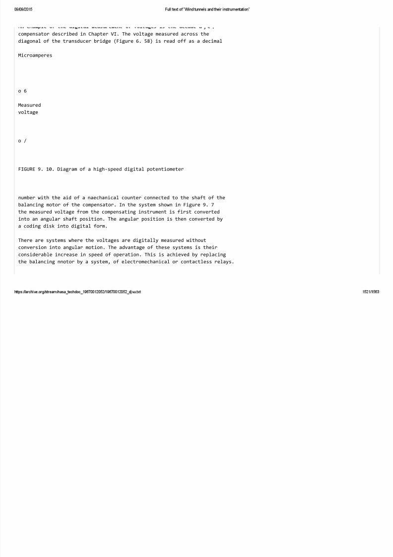
compensator described in Chapter VI. The voltage measured across the

diagonal of the transducer bridge (Figure 6. 58) is read off as a decimal

Microamperes

o 6

Measured

voltage

o /

FIGURE 9. 10. Diagram of a high‐speed digital potentiometer

number with the aid of a naechanical counter connected to the shaft of the

balancing motor of the compensator. In the system shown in Figure 9. 7

the measured voltage from the compensating instrument is first converted

into an angular shaft position. The angular position is then converted by

a coding disk into digital form.

There are systems where the voltages are digitally measured without

conversion into angular motion. The advantage of these systems is their

considerable increase in speed of operation. This is achieved by replacing

the balancing nnotor by a system, of electromechanical or contactless relays.

 

575

A circuit diagram of a high‐speed digital potentiometer is shown in

Figure 9. 10. This system was developed by the Lewis Aeronautical

Laboratory (NASA) for the multipoint measurement of thermocouple

signals, but is also suitable for measuring signals from strain gages /4/.

The instrument is designed for measuring voltages ranging from — 10

and — 40 millivolts in 72 channels during 48 seconds. The temperature

is read by comparing a compensating voltage with the measured voltage.

The difference between these voltages is amplified, and the output voltage

from the anaplifier is used for changing the compensating voltage until it

equals the m.easured voltage. Twelve fast‐acting relays switch on 12

resistors in the compensating circuit, for balancing the potentiometer.

The figures in Figure 9. 10 denote the current in microamperes passing

through the corresponding resistors when the relay contacts, in series with

the resistors, close. The sum of these currents pass through a 10 ohm

resistor for producing the compensating voltage.

Different relay switching combinations give any compensating voltage

between and 9.99 millivolts in steps of 0.01 millivolts. To obtain the

necessary voltage balance, the resistors are switched from left to right

by a step selector incorporated in a circuit consisting of 12 thyratrons.

Immediately after the first [selector] contact is closed, the relay contacts

to the input of the amplifier are broken, giving a positive pulse if the

balancing voltage is less than the unknown voltage, and a negative pulse

if it is greater than the unknown voltage. A positive pulse fires the

thyratron connected by the selector to the output of the amplifier, and

switches in via an intermediate relay the first resistor. If the balancing

voltage is greater than the unknown voltage, the first thyratron is not fired

 

  ,

energized. The same process takes place for each of the 12 steps. At the

end of the cycle, some thyratrons are conducting, the contacts of the

relays connected with them are closed, and the potentiometer is balanced.

The voltage is read from, the conducting or nonconducting condition of each

of the 12 thyratrons, which serve as a register.

The relay in the plate circuit of the thyratron gives the information to a

paper‐tape puncher. For the puncher to be operated constantly, two

thyratron assemblies are provided, one for obtaining the information from

the potentiometer, and the second for simultaneously transmitting to the

puncher the information received in the previous read‐down. The thermo‐

couples are switched successively into the circuit via a separate step

selector switch. Figure 9. 11 shows the simplified block diagram of the

system. The moment the amplifier transmits the information to the upper

thyratrons, the lower thyratron register transmits to the relay register

the information recorded during the previous read‐down. The information

in the registers is erased by momentarily shorting the plate supply voltage

of the thyratrons, thereby enabling the lower register to receive new

information from the amplifier. The relay register decodes the inform.ation

recorded on the thyratron register as a 1, 2, 2, 4 code into a natural

binary code. The programmer transmits to the tape, in the necessary

sequence, the information frona the relay register and from the channel

coder. The channel coder punches on the tape the num.ber of the channel

corresponding to the given read‐down.

576

Method of dynamic compensation

 

 

value with a compensating value changing linearly with time. The

compensating value is given as a sum of a certain number of pulses, each

corresponding to a given interval of change in the measured value. Usually

this interval is taken equal to the resolving capability of the measuring

instrument. The number of intervals corresponding (to an accuracy of 1

interval) to the measured value are read off by an electronic pulse counter

and recorded in a memory device (for instance on a magnetic tape or drum).

 

Source of

compensating

voltage

r

Thyratron

register

*•

Relay

register

~l

 

\

Comparator

Amplifier

i‐J^

 

J^

i

1

i\

 

1 A

/

I

Thyratron

register

♦

Relay

register

ii

 — Scanner

 

I

■

‐h

^ —

II

Coder

 

/

,"l,‐,r,,‐,‐^1 M^

1

 

 

Programmer

'*

Control

device

Tape puncher

 

FIGUI?E 9. 11. System for transmitting data from an automatic potentiometer to a puncher.

An exaxnple of a dynamic compensation system for measuring voltage

is given in Figure 9. 12. The voltage from one of the transducers (2)

is fed through amplifier (3) to zero indicator (4), which is supplied with

a saw‐tooth voltage from saw‐tooth voltage generator (10). The generator

is started by a pulse from control circuit (1). Zero indicator (4) compares

the amplified voltage ui from amplifier (3) with the momentary saw‐tooth

voltage U2 . When voltage u, and ui are equal, the zero indicator produces

a pulse, which is fed to gate (5) and data output pulse generator (6). Until

a pulse appears from the zero indicator (4), gate (5) is set by a control pulse

to a state where clock pulses from generator (9) pass through the gate to

binary counter (8). A pulse from the zero indicator (4) closes gate (5),

inhibiting the passage of these pulses to counter (8). At the same time, the

same pulse from zero indicator (4) starts data output generator (6) for

transmitting the pulses recorded by counter (8) to the memory device (7),

and subsequently resets the counter to zero. When the next control pulse

appears the saw‐tooth generator (10) starts again, gate (5) passes clock‐

pulses to counter (8), and the measuring cycle is repeated.

Thus the number of pulses recorded by counter (8) is proportional to

the voltage from transducer (2). The recording in the long‐term

577

memory (7) takes place between two measurem.ents. Each pulse

corresponds to a known small interval of voltage, and therefore knowing

the total number of pulses, it is easy to determine the measured voltage.

 

";

t

Control

"t

K,

in

 

r t

Gate

Clock pulses

Clock pulses passing

through gate

_ | 1^ Closed

" jiiiijt

'■■■ ■"'

FIGURE 9. 12. System for measuring a voltage as a number of pulses. 1 — control circuit;

2 — transducers; 3 — amplifiers; 4— zero indicator; 5 — gate; 6 — data output pulse genera‐

tor; 7 — long‐term memory; 8 — electronic counter; 9 — clock‐pulse generator; 10 — saw‐

tooth voltage generator; 11 — scanner.

The electronic binary counter consists of series ‐connected cells

(triggers) each corresponding to a binary bit. The on condition of each

cell represents a 1, while the off condition represents a 0. As pulses

are fed to the input of the counter, they are transmitted from one cell

 

  , .

pulses sent to the counter can be read off from the state of the cells.

Thus, for instance, if an on cell is represented by a dark rectangle and

/«?« 512 256 128 Bit 32 id 8 « 2 1

1111111111

10 1110 110 1=1261

FIGURE 9. 13. Electronic counter.

an off cell by a white one, then the display of the binary counter, as shown

schematically in Figure 9.13, will be 10011101101, i.e., the decimal

number 1261. For multipoint m^easurement, it is not required to count

578

the number of pulses in each measuring channel with separate electronic

counters. Due to their high speed of operation, one counter can successively

count the number of pulses in each channel and give this number as a binary code

 

  .

of 10^ cycles, it is possible by dynamic computation to record on magnetic

tape, during one second, 1000 values to an accuracy of 0.1%. To accomplish

this, a high‐speed electronic switch (11) should be placed at the amplifier

input (Figure 9. 12). Electromechanical switches can be used for measuring

up to 100 channels per second.

Compensating

pressure

FIGURE 9. 14. Converting compensating pressure

into a pulse train. 1 — pressure‐switch diaphragm;

2 — reservoir; 3— bellows; 4 — spring; 5— induc‐

tive pick‐up; 6 — amplifier; 7 — servomotor; 8 —

micrometric screw; 9 — nut; 10 — support for springs;

11, 12— levers; 13 — unloading pistons; 14— light

source; 15 — photo element.

The pulse method was specially developed in the Lewis Aeronautical

Laboratory, NASA (U.S.A.), where several thousand measurements are

made daily in wind tunnels designed for testing turbojet engines. In this

laboratory, naultipoint measurements are made by comparing with one

common conapensating pressure, which is cyclically changed from zero

to maximum. The compensating pressure, in its turn, is accurately

measured by one of two methods: 1) with the aid of a compensating

manometer producing a pulse train, each pulse corresponding to a fixed

small interval of movement of the manometer balancing element, or,

which is the same, to a fixed interval of change in pressure / 5/ ; 2) by

using equipment providing a pressure changing linearly with time. In this

case, the number of pulses generated by a clock‐pulse generator during

 

579

an interval of time are counted. These represent change in pressure

from a fixed initial value up to the measured quantity /6/,

An arrangement for measuring pressure using the first method is shown

in Figure 9. 14. The primary pressure measuring element is pressure

switch with a sensitive diaphragm (1) (Figure 5.56, Chapter V). For

simplicity, only one switch is shown in the figure, but the actual number

equals the number of pressures measured. The measured pressure p,‐ is

applied to one side of the diaphragm. The other side of the diaphragm is

connected with reservoir (2), in which is created a varying compensating

pressure. Initially, a vacuum is created in reservoir (2). As the measured

pressure is greater than the pressure in the reservoir, the diaphragm is

deflected and closes an electrical contact. The reservoir is connected to

an accurate manometer, which sends electrical pulses, with increasing

pressure in the reservoir, to a circuit closed through the diaphragm.

Each pulse corresponds to an increase in pressure of 0.25 mm Hg. The

pulses are counted until the pressure in the reservoir equals the measured

pressure. At this moment, the diaphragm opens its contact, and the pulses

stop reaching the counter which is connected to the diaphragm. The

measured pressure in mm Hg is eqaul to 0.25 n, where n is the number of

recorded pulses. The pressure in the reservoir continues to rise to a value

slightly higher than the highest measured pressure, after which a vacuum

is again created in the reservoir. A measuring cycle lasts 10 seconds.

A null‐instrument is used for measuring the compensating pressure and

for sending pulses. It consists of a bellows (3), whose movable cover is

connected with two flat cantilevered springs (4), and a differential trans‐

former (5), sensitive to movements of up to 0.00025 mm. As the pressure

 

  ,

springs move upward. As a result, a signal is induced in transformer (5),

which is amplified in amplifier (6), giving a voltage to servomotor (7). The

latter rotates micrometric screw (8). Nut (9) moves support (10), on

which are fixed springs (4), until the force exerted by the springs equals the

pressure on the cover of the bellows. This is carried out with the aid of

levers (11) and (12), which form, together with the moving support (10), a

parallelogram. This arrangement moves support (10) towards the bellows

by about the amount of deformation of the spring, and prevents the bellows

from, moving sideways. A piston (13) relieves nut (9) from the forces

acting on the bellows.

Servomotor (7) rotates the micrometric screw through a pair of gear

wheels. The gear wheel on the axis of the screw has 180 teeth. The

stiffness of springs (4), the area of bellows (3), the transmission ratio

of lever (11), and the pitch of the screw are chosen in such a way that a

turn of the screw by 2° corresponds to a change in pressure of 0.25 mm Hg,

Each of the 180 teeth of the gear wheel, when turning, interrupts a ray of

light between source (14) and photoelement (15).

Figure 9. 15 shows a block diagram of a pressure recorder, the

measured pressures pi p„ are fed by tubes to the diaphragm heads.

The electrical pulses generated by the photoelements of pressure meter (3)

are fed simultaneously via the closed contacts of all the diaphragm heads

(2) to the recording heads (4) of a short‐term magnetic memory. The

latter is a bronze drum with an external diameter of 300mm and a length of

100 mm. During the changing pressure cycle in the reservoir, the drum.

580

 

rotates uniformly. Recordings are made by magnetizing the ferromagnetic

coating on the surface of the drum which is at the given moment under the

recording head. The clearance between the recording head and drum

surface is 0.025 ixun.

L,

m

 — JtfTl

^ LLTl

I ^Bell

Bellows

7

Throttling valve [^ II

 

5^

4

Short‐term

memory

‐ s

10

~o

IE

 

FIGURE 9. 15. Diagram of a multipoint pressure measuring system. 1 — reservoir in which is

created the compensating pressure; 2— diaphragm pressure switch; 3 — pressure meter with pulse

generator; 4— magnetic recording heads; 5 — magnetic drum; 6 — scannei; 7 — electronic counter;

8 — coding and decoding; 9 — printer; 10— tape puncher; 11— control panel; 12 — pressure and

vacuum control.

The recording head is an open permalloy core, wound with a coil having

a small number of turns (to reduce inductance). During the passage of a

pulse, a field is created in the core gap which magnetizes the ferro‐

magnetic coating. The recording heads are uniformly placed around the

drum in 21 rows with 5 heads in each row. Thus, the drum can record

pressure from 105 measuring channels. The pulses are recorded on 85%

of the circumference of the drum as separate tracks for each measured

pressure. The maximum number of pulses is 400. The drum has two

speeds: a low speed of one rotation per 12 seconds for recording pulses;

a high speed of 1.5 sec per revolution for reading down the pulses from the

drum to the electronic counter. The counter is in turn switched by a

scanner to the recording head, which is switched beforehand for readings.

The pulses are read down in reverse order from that in which they were

recorded. As the magnetized sections of the drum pass under the head,

a voltage pulsfe is Induced in the head which is amplified and fed to an

electronic counter.

The data from the electronic counters are fed to a special relay

register, where the numbers are held for punching on paper tape and

for being printed in a form suitable for a computer. At the same time.

581

 

such data as the channel number, computer instructions, experiment

number, record number, date, and other necessary data are also recorded.

A characteristic example of using dynamic compensation methods is the

centralized measuring system at the Lewis Aeronautical Laboratory (NASA)

/6/. This system is the intermediate link between 9 wind tunnels and

electronic computers. The data previously recorded on intermediate

memory devices are transmitted as pulses over telephone wires to a

central encoder and are recorded on magnetic tape during the time the

necessary stream conditions are established for the next measurement.

Four types of data are recorded on the magnetic tape:

1) data common to the given job, e.g., read‐down number, record,

number, barometric pressure, date, etc.;

2) the pressure at 300 points measured with pressure switches;

3) voltages from 200 channels measured with thermocouples, and

voltages from strain gages of wind‐tunnel balances and potentiometers.

13

 

/;

10

t‐

9

 

FIGURE 9.16. Centralized data collection system— Lewis Aeronautical Laboratory

(NASA). 1 — pressures; 2 — voltages; 3— frequency pulses; 4— magnetic core matrix;

5,6 — electronic counters; 7 — central encoder; 8 — magnetic‐tape recorder; 9 — electro‐

nic computer; 10 — printer; 11 — graph plotter; 12 — common information (model no.,

test no. , etc.); 13 — encoder control.

indic?ating shaft positions. The voltages are recorded at a speed of 20

channels/sec using a system similar to that shown in Figure 9.12;

4) pulse frequencies produced by naagnetic pickups on tachometers

measuring the r.p.m. of the tested engine, and magnetic pickups on

flow meters measuring the amount of fuel entering the engine.

 

  ,

the central encoder, and output devices is shown in Figure 9. 16.

582

The connections are made with relays, which automatically switch the

different circuits during data recording. The dynamic compensation method

used in the given system differs fromi the system shown in Figure 9. 15 in

that instead of using a manometric instrument for controlling the

compensating pressure in the reservoir, a device providing a pressure

changing linearly with time is used. A magnetic matrix is used for

recording instead of a drum and the pulses recorded represent fixed intervals

of time instead of fixed interval pressure. The linearly changing pressure

is obtained by using a throttling nozzle which gives a constant critical flow.

FIGURE 9, 17, Arrangement for measuring pressure and recording the pulses in a magnetic core

memory, 1 — reservoirwiihlinearly changingpressure: 2 — diaphragm pressure switches; 3 —

clock‐pulse generator; 4— readout‐pulser; 5 — input from binary‐decimal electronic counter;

6 — matrix; 7 — output register; 8~gates.

By recording the moments corresponding to the known lowest pressure p, ,

and the known highest pressure pj , it is possible to determine the pressure

p^i at any internaediate moment. The time is measured using a 1000 cps

clock‐pulse generator. The number of pulses from the moment the pressure

begins to change in the reservoir to moments ft, txu h is counted by electronic

counter (5) (Figure 9.17). A magnetic core nnatrix is used for storingthe pulses

 

583

accumulated during time /,i in each of the 300 m.easuring channels. Each

magnetic core consists of a miniature ceramic bobbin wound with a tape of

m.agnetic material 0.12 mm thick. Through a hole in the bobbin three wires

pass for the voltage pulses.

The memory qualities of the cores are based on their magnetic

rectangular hysteresis loop. A minimum current / through one of the

wires is required to change the magnetic position of the core. With a

current of i‐j‐/, the core remains in its initial magnetic condition. How‐

ever, if two current pulses of^/ pass through two wires, the magnetic

flux caused by these two currents is summed and the magnetic condition of

the core changes. Thus, the core will remember the coincidence by

changing its magnetic condition. The cores are placed in horizontal and

vertical rows in the form of a matrix. Sixteen cores in one vertical

column form one information channel and can store a 4 digit decimal number

(a 16 digit binary number). To store the data of 300 channels, 300 vertical

columns are required.

A vacuum tube is connected to each vertical colunan. The tube passes

current only when a positive voltage is applied to the control grid. The

tube is controlled by the diaphragm pressure switch of the given measuring

channel. A horizontal wire passes through each of the 16 cores of one

column, and the current through the wire is controlled by the 16 bits from

the binary‐ decimal electronic counters. The function of each bit from, the

counter is to control the transmission of a pulse of ‐^/ along the horizontal

 

wire to the corresponding core. If the counter position contains a unit of

information, it will pass a pulse of‐g‐/ into one core of each of the 300

channels.

At the moment the measuring cycle starts, the 1000 cps clock‐pulse

generator switches on. The generator sends pulses to the electronic

counter and to each of the 300 tubes connected with the diaphragm

pressure switches. When the pressure in the reservoir equals the pressure

measured by the given pressure switch, the diaphragm opens its contact

and a signal is transmitted to the tube connected to this pressure switch.

With the next pulse from the generator, this tube passes a current pulse

of g‐/ into the 16 cores of the corresponding channel. Simultaneously,

the electronic counter sends pulses of ‐s‐^ along the horizontal wires

connected to those positions in the counter storing bits. Those cores

of the given channel receiving coincident pulses along the horizontal and

vertical wires change their magnetic condition, and thus remember the

number of pulses stored by the electronic counter when the tube was

switched on.

Those cores not receiving coincident pulses remain unchanged. After

the contacts' of all the diaphragm pressure switches have operated, a

signal is automatically sent to read down the information stored in the

matrix memory. The informiation is read down of a speed of 20 channels

per second by sending a current pulse larger or equal to / through each

vertical column via pulser (4). A second electronic counter (output register)

(7) records the voltage pulses appearing on the third wire of each horizontal

 

 

row of the matrix. These pulses are induced by changes in the magnetic

flux of the core and pass the recorded values to the central encoder. At

the end of read‐down the system, is reset to its initial condition and is

ready to receive the next measurement.

Engine r.p.m. and fuel output are recorded by electronic counters

counting the number of pulses produced by magnetic tranducers from

tachometers and flowmeters (Figure 9. 18) during an interval of 10 seconds.

FIGCJRE 9. 18. Measuring r. p. m. and flow.

1~ pulse transducers connected to a rotating element; 2 —gates;

3 — electronic counters; 4 — 10 sec interval generator; 5~central

register; 6 — read‐down control; 7 — magnetic tape recorder.

All the instrument indications are recorded after establishing the

conditions in the tunnel. When the operator presses a read‐down button,

all the instruments of the given tunnel are automatically switched to the

corresponding output device for recording on magnetic tape. The cycle

continues for 10 seconds, and when terminated, a light signal is switched

on in the control room of the given wind tunnel, allowing conditions to be

changed.

The time required to finish the recording cycle and prepare the

necessary circuits for recording the next point is about 15 seconds. If during

this time the operator of another wind tunnel presses a corresponding

button, the beginning of recording signals from this tunnel is delayed

 

  .

recording period, such delays remain unnoticed by the operator.

Depending on the type of experiment and the number of wind tunnels

working simultaneously, the data measured can be either directly fed

to electronic computers or accumulated on magnetic tape for further

processing. In addition, the primary values recorded on magnetic tapes

are printed on electric typewriters and recorded on high‐speed graph

plotters placed in the wind‐tunnel control rooms.

585

§45. PROCESSING THE MEASURED DATA

ON COMPUTERS

Data processing on an analog installation

Figure 9. 19 shows a block diagram of an electronic analog installation

at the Wright Brothers Scientific Research Center (U. S. A.) for automatically‐

processing the data from strain gages used for measuring stresses and

pressures 111 .

Channel

Transducers amplifiers

 

Load

Model

>‐ 3

Scale

factors

Torque

Sign inverter

and Adders

discontinuities

Stress

 

  . .

at the Wright Brothers Research Center.

The least squares method is used to determine the torque AJ,, and the

stress y, acting on the model installed on pivoted strain‐gage balances .

The device computes according to the formulas discussed in Chapter VT

(page 409)

AJi, = fljiAui ‐)‐ anCiU‐2 + ajsAua ■+ . . . ,

where Aui, Au2, • ■ • are the voltages from the strain‐gage bridges placed in

different sections of the beam. The measuring system of each transducer

operates with an a. c. carrier frequency. Filters at the output of the

information channels filter out the carrier frequency and d.c. signals

are received proportional to the measured values of Au,‐. The d.c. signals

are summed in operational amplifiers. Before summation, the signals

from different channels are multiplied by "weight" coefficients as

determined by the constants of the equation. These coefficients depend

on the design of the balances and the model, inserted by potentiometers

at the input of the operational amplifiers, and are easily controlled.

Correction factors are also inserted into the adders.

The pressure factor is determined by

^ Pa

Pa

 

.

1680

586

which is converted to

where p is the measured pressure at a given point, p„ is the static

pressure in the incoming stream, p^ is the barometric pressure.

mi = — can change during the day but is constant for the given test.

Pa

nii =— ‐IT is a constant for the given tunnel, mi = ‐^ is a combination

"M Pa,

of variable values constant for the given series of tests.

The above equation is solved by modulating the voltage of the carrier

with the amplitude of the signal from the pressure transducer. The

modulated signal is rectified, multiplied by coefficients m, and mj in the

information channel, and then summed in the operational amplifier with

a voltage proportional tonij. At the output of the adder, a voltage

proportional to the pressure factor is obtained.

 

 

processes having a frequency up to 500 cps.

Processing the measured data on digital computers

The processing of data from wind‐ tunnel measurements differs by two

specific characteristics. Firstly, the total amount of processed data is

large. Consequently, the data input and output devices of the computer

must have a large throughput capacity, and the internal mem.ory must

have a large storge capacity. Secondly, the necessary computations are

sim.pler than those required by most analytical problems. Therefore, high

computing speed is not a major requirement. Because of the above‐

mentioned reasons, in addition to universal electronic computers, special

machines are found with fixed programs, adaptable for solving problems

of a definite type. Special machines are usually simpler and less expensive.

The drawback of computers with fixed programs is that even small changes

in the computing sequence (which are sometimes met when processing data

from, different types of measurements) call for readjusting the computer.

Where relatively simple computations are required, but the computing

program cannot be given beforehand, small computers are used. Thus,

for instance, in the Lewis Aeronautical Laboratory (NASA), a small

IBM‐ 604 computer is used for processing the data of m.ultipolnt pressure

and temperature measurenaents of jet engines /8/. The basic data and

instructions are fed from punch cards. The results are produced on punch

cards at a speed of 100 cards per minute.

A property of the system is that the computer instructions are

automatically fed in directly during the tests. With each read‐down of

temperature and pressure, separate instructions are given to the

computer in the form of an operational code. Operational codes are

 

 

recorder, simultaneously with read‐down. Thus, the computer can

automatically change the computing sequence in accordance with the

1680

587

instructions transferred to the computor following each read‐down. This

simplifies the processing of data obtained from different experimental

objects and instruments.

The method of processing the measured data on an IBM‐604 computer

using punch cards can be seen in Figure 9. 20, where pressures are

measured with the aid of a multipoint digital recorder.

FIGURE 9. 20. Automatic data processing with a digital computer in the Lewis Aero‐

nautical Laboratory. 1 —reference pressure; 2 — tested engine; 3 — pressure in engine;

4 — paper tape: 5 — reader; 6 — codex; 7 — puncher; 8 — blank punch cards; 9 — punch

cards with additional punchings; 10 — sorter; 11 — computer; 12 —digital pressure recorder.

The recorder writes on a magnetic drum the digital values of the full

pressure at 6 points in front of the engine, the static pressure at 6 points

on the wind‐tunnel walls, the pressure at 6 points on the engine, and

3 reference pressures against which the full pressure is compared.

 

The computer determines the average value of the full pressure,

corrects for the losses between the sections where the pressure tranducers

are placed and the input section to the engine, finds the average value of

static pressure, and divides the static pressure and each of the pressures

measured in the engine by the corrected full pressure.

The data from the digital recorder are punched onto paper tape and

contain the coded digital values measured, the channel number, and the

operating instructions. These data are transferred for each meesurement

from the puncher to a separate punch card. The punch cards are fed via

a sorter to the computer.

Additional data, for instance, the calibration coefficients and corrections,

are put into the computer with the aid of additional punch cards. The sorter

compares the numbers punched on the main punch cards with the numbers in

588

the auxiliary punch cards and automatically puts the latter into the

appropriate places between the main punch cards.

Figure 9. 20 shows the sequence of feeding the main auxiliary punch

cards to the computer and the marking of the code of the operational

instructions. The first punch card is an auxiliary one and contains

information on the calibration coefficient and support pressure. The code

punched on this card instructs the machine as to the use of this information

for further computation. The next punch card, referring to channel 01, is

punched with a code 1, 3, and on those punch cards referring to channels

02 and 03, with code 3. Code 1, 3 instructs the machine to begin the

 

  ,

continued. The card in channel 03 is followed by an auxiliary card, coded

8, 9. Code 8 instructs the machine to divide the summed pressures from

channels 01, 02, and 03, by three, and to punch out the results. Code 9

instructs the machine to record the computed average pressure from all

the following punch cards. This is necessary because at this point the

complete limited capacity of the memory is used up.

The next card is an auxiliary card, coded X, 12, 1, 2, 3, 8, and 9. The

machine does an operation corresponding to the logical sum of the

instructions of this compound code. Code 12 instructs the machine to

operate with the average pressure of channels 01, 02, and 03. The

appropriate corrections are inserted into the average value, and the new

pressure is kept for comparing with the subsequent pressure according to

instruction code 2. The values of the full pressures are corrected by the

corrected value of the support pressure as given on the punch card, and

the next punch card with the code X gives a new calibration coefficient for

channels 04 to 09. The code on subsequent cards instructs the machine on

making further computations in the described order.

 — Jj

 

\ 7 \\ S \

12

.CD zn

Compu

ing center

FIGURE 9. 21, System for automatic data processing during an experiment. 1 —wind‐tunnel

balances; 2 —digital converters for wind‐tunnel balances; 3 —multipoint manometer; 4 —

digital converter for manometer; 5 — auxiliary data input; 6 —controller; 7 — punchers;

8 — readers; 9 — buffer memory; 10 —print‐out of primary data; 11 —graph recorder of advance

data; 12 ‐Datatron computer; 13 — print ‐out of processed data; 14 —distributor; 15— graph

plotter of final data.

589

 

 

Figure 9. 21 shows an automatic system for processing data during the

experiment intended for serving two supersonic wind tunnels at the

California Institute of Technology (U. S. A.). In these tunnels, the forces

acting on the model are measured by six‐component hydraulic and strain‐

gage balances using automiatic compensators. The output values of the

balances represent the angular position of shafts. The angular positions

are converted to digital form by relay converters.

Register V Readout

device

FIGURE 9. 22. System for automatically plotting graphs from digital data. 1 — table with

paper sheet; 2 — guide; 3— carriage; 4 — lead screw for pen; 5— pen; 6 — lead screw for

carriage; 7, 8 —servomotors; 9 —analog ‐to‐digital converters.

The distribution of pressures in the model is measured by a system

described in Chapter V. Selector valves connect, in turn, all the openings

in the drained model with one manometer, whose indications are measured

by an automatic compensator and converted into digital form.

The values of the forces and pressures, together with data referring

to the position of the model, the Mach number, experiment number, and

 

  ,

at a speed of 60 digits per second. The punched tape is fed at once to the

computer reader.

The control room of the wind tunnel is placed remotely from the

computing center, and the data read frorn the punch tape are fed to the

computer through wires. The data processed by the computer are recorded

on punch tapes and fed back to the control room where they are tabulated.

At the same time, graphs are plotted from the data. The readers, punchers,

graph plotters, and printers can be interconnected by different methods

depending on the test programs. For instance, with force measurements,

when the amount of measured data is comparatively small, but the

processing is more complicated, it is possible to prepare two identical

590

punch tapes with primary data. One is immediately fed to the comiputer,

while the other is used for operating a tabulator or an X‐Y plotter. With

combined tests, where the forces and pressures are measured

simultaneously, one tape records the indications of the balance, while the

other records the indications of the manometer.

The printing of tables and plotting of graphs are operated by the given

system during tests, thus allowing the senior engineer to monitor the

experiment. This is very important when doing basic research of new

phenomena.

( f‐

 

^

Cs^

i

br

o^^p

r _L_ 2

I

 

Don

T7

FIGURE 9. 23, A digital‐to‐analog converter for an automatic X— Y plotter.

1 — amplifier; 2 — balancing motor; 3 — rheostat: 4 — potentiometer con‐

trolled by relays.

Figure 9. 22 shows an arrangement of an automatic X‐Y plotter for

converting the digital numbers coded on paper tape to a continuous pen

motion. The X‐Y plotter can choose data from different measuring

channels and plot several of them as a function of a parameter measured

in any channel. Above the paper (1), parallel to the X‐axis, a carriage (3)

moves on guides (2), The carriage is driven by screw (6), The carriage

moving along the Y axis, carries a pen (5), with an electromagnetic marker.

The ruler and the pen are driven by balancing servomotors (7) and (8),

connected to digital‐to‐analog converters (9), The digital values read from

the paper tape are transmitted as pulses to the X‐Y registers from where

they are fed to the converters (9),

Each converter (Figure 9, 23) consists of a balanced Wheatstone bridge,

two branches of which are formed by a group of fixed resisters. The

resisters are switched into the branches by a systeni of electromagnetic

 

.

corresponding lead screw of the X‐Y plotter. When both bridges reach

591

balance, the electromagnetic marker frees the pen, which falls for a

momient on the paper, making a dot. The pen is then raised, the Y relay

register receives signals from the other channel, and the pen is moved to

a new position, making another dot.

BIBLICX3RAPHY

1. Kitov,A.N. and N. A . Kr init s kii. Elektronnye tsifrovie

vychislitel'nyemashiny (Electronic Digital Computers).— Moskva,

Fizmatgiz. 1961.

2. Leb e d ev, S. A. . Elektronnye vychislitel'nye mashiny (Electronic

Computers).— Izd. AN SSSR. 1956.

3. Scholes , J. F. M. The Automatic Handling of the Experimental Data in

Wind Tunnels. — British Communications and Electronics, Vol. 4,

No. 10. 1957.

4. Smiith,R.L. A High‐Speed Potentiometer for Recording on Punched

 

  , , . . .

5. Sharp, E.M. A Digital Multiple Point Pressure Recording System. ‐ISA

Proc, Vol.7, 1952.

6. Sharp, E.M. An Automatic Data Recording System for Aeronautical

Research — IRE Trans. Instrum., Vol.6, No. 7. 1957.

7. Haneman, V.S. Automatic Reduction of Wind Tunnel Data. — Aeron.

Engns. Rev., Vol.12, No. 2. 1953.

8. Rawlings , J.H. Mechanized DataHandling.— ISA Proc, Vol.7. 1952.

592

$ 9.00

NASA TT F‐346

Cover printed in Jerusalem, Israel TT 66‐51026