functional morphing for manufacturing ......functional morphing for manufacturing process design,...
TRANSCRIPT
FUNCTIONAL MORPHING FOR MANUFACTURING PROCESS
DESIGN, EVALUATION AND CONTROL
by
Liang Zhou
A dissertation submitted in partial fulfillment
of the requirements for the degree of
Doctor of Philosophy
(Mechanical Engineering)
in The University of Michigan
2010
Doctoral Committee:
Professor Shixin Jack Hu, Chair
Professor Gregory M. Hulbert
Associate Professor Jionghua Jin
Thomas B. Stoughton, General Motors

Liang Zhou
©
All Rights Reserved
2010

ii
ACKNOWLEDGMENTS
I would like to thank my advisor, committee members, colleagues, friends, and
family for their help and support. Without them, I would never have been able to finish
this dissertation.
Sincere gratitude goes to my advisor and chair Professor S. Jack Hu for his
continuous encouragement and help through my Ph.D. studies. His vast knowledge,
vision and support were fortunes to me during the past 5 years. Professor Hu taught me
how to think critically, and to write and express myself clearly.
I would also like to extend gratitude to my other committee members, Professor
Jionghua Jin, Professor Gregory M. Hulbert and Dr. Thomas B. Stoughton for their
constructive suggestions and valuable discussion while in pursuit of my studies. I
especially appreciate Dr. Stoughton‟s vision and support through the discussions of my
research.
I am also grateful to Dr. Pei-Chung Wang, who opened the door of automotive
manufacturing for me and gave me tremendous help in both research and life. My
interaction with Dr. Wang benefited me both professionally and personally.
I also want to express my acknowledgment to General Motors Corporation for the
financial and technical support of my research, especially Dr. Susan Smyth, Dr. Jeff
Abel and Dr. Roland Menassa who have always offered their constructive support. In
iii
remembrance, I would also like to thank Dr. Samuel P. Marin whose insight and
kindness have set a goal I wish to achieve in my life time. I also want to express my
thank to Dr. Raymond Sarraga, Dr. Wayne Cai, Dr. Chih-Cheng Hsu, Daniel Hayden,
John Fickes, Steve Koshorek, Dr. Wu Yang and all the colleagues I have worked with
for their support and help throughout these years.
Special thanks to Dr. Guosong Lin and Dr. Hui Wang who have worked with me
closely on my research. They offered me much help and encouragement to overcome
technical obstacles I have faced. I am deeply indebted to them.
My gratitude also goes to my friends and colleagues in Hu-Lab, Dr. Tae Kim, John
Wang, Jingjing Li, Sha Li, Xiaoning Jin, Shawn Lee, Hai Trong Nguyen, Saumuy
Suriano, Chenhui Shao, Robert Riggs, Taylor Tappe, Vernnaliz Carrasquillo, and
former colleagues Dr. Yuanyuan Zhou, Dr. Xiaowei Zhu, Dr. Jian Liu, Dr. April Bryan,
Dr. Luis Eduardo Izquierdo, Dr. Hao Du, Dr. Ugur Ersoy, Dr. Joenghan Ko and Dr.
Jianpeng Yue for providing a stimulating and open environment for thinking and
research. Special thank also goes to Constance Raymond-Schenk and Kathy Brotchner
for their continuous administrative help and support.
Most importantly, none of these would have been possible without the love and
support from my family. I want to express my greatest appreciation to my parents for
their faith in me and unconditional love, concern and support. I also owe gratitude to
my fiancé, Xiaohong Zhang, for the love, support and happiness she has brought to my
life.
I owe my gratitude to all those people who have made this dissertation possible
and made my doctoral study experience possible.
iv
TABLE OF CONTENTS
ACKNOWLEDGMENTS .......................................................................................... ii
LIST OF FIGURES .................................................................................................. vii
LIST OF TABLES ...................................................................................................... xi
ABSTRACT ........................................................................................................... xii
CHAPTER 1 INTRODUCTION ..............................................................................1
1.1. Motivation .................................................................................................1
1.2. Literature Review......................................................................................5
1.2.1. Image Transformation ....................................................................5
1.2.2. Morphing in Process Design, Evaluation and Control ...................6
1.2.3. Summary of Literature Review ....................................................10
1.3. Research Objectives ................................................................................10
1.4. Organization of Dissertation ................................................................... 11
References ........................................................................................................13
CHAPTER 2 FUNCTIONAL MORPHING BASED EVOLUTIONARY
STAMPING DIE DEVELOPMENT ..............................................19
2.1. Introduction .............................................................................................20
2.2. Die Face Morphing Algorithm ................................................................22
2.2.1. Free-Form Representation for Part and Die .................................24
2.2.2. Part-to-Part Mapping by FFD Based Transformation ..................25
2.2.3. Die-to-Die Morphing ....................................................................31
2.2.4. Consideration on Trimmed Surfaces ............................................31
2.3. Case Study ..............................................................................................33
2.3.1. 2D Study on Stamping U-shaped Channel ...................................33
2.3.2. 3D Case Study on Cup Drawing ..................................................36

v
2.3.3. Mapping of Trimmed Surface ......................................................39
2.4. Conclusion ..............................................................................................42
References ........................................................................................................42
CHAPTER 3 FUNCTIONAL MORPHING BASED FORMABILITY
ASSESSMENT IN STAMPING DIE FACE MORPHING USING
STRAIN INCREMENT METHOD ................................................44
3.1. Introduction .............................................................................................45
3.2. State-Of-The-Art .....................................................................................46
3.3. The Strain Increment Method .................................................................48
3.3.1. Geometric Mapping by Free-Form Deformation .........................48
3.3.2. Overview of the Strain Increment Method ...................................49
3.3.3. Mapping of FE Mesh to Geometry ...............................................50
3.3.4. Strain Increment from Displacement ...........................................52
3.3.5. Bending Energy and Strain Gradient Functions ...........................55
3.4. Case Study ..............................................................................................58
3.4.1. 2D U-shaped Channel Stamping ..................................................58
3.4.2. Generation of New Die Surface ...................................................59
3.4.3. Strain Prediction by Strain Increment Method .............................60
3.4.4. 3D Case Study on Cup Drawing ..................................................61
3.5. Conclusion ..............................................................................................64
References ........................................................................................................65
CHAPTER 4 FUNCTIONAL MORPHING IN MULTI-STAGE
MANUFACTURING AND ITS APPLICATIONS IN
HIGH-DEFINITION METROLOGY BASED PROCESS
CONTROL ........................................................................................68
4.1. Introduction .............................................................................................69
4.2. Modeling of Surface Changes Using Functional Morphing ...................72
4.2.1. Feature Extraction ........................................................................73
4.2.2. Functional Morphing for Surfaces ...............................................74

vi
4.2.3. Morphing Based Multi-stage Variation Modeling .......................79
4.3. Applications of Functional Morphing in Machining Process Control ....82
4.3.1. Inter-stage Process Adjustment ....................................................82
4.3.2. Backward Morphing Based Process Monitoring ..........................84
4.3.3. Process Tolerance Design ............................................................85
4.4. Case Study ..............................................................................................86
4.4.1. Experimental Setup ......................................................................86
4.4.2. Functional Morphing Between Stages .........................................88
4.4.3. Inter-stage Process Adjustment ....................................................89
4.4.4. Backward Morphing Based Process Monitoring ..........................93
4.5. Conclusion ..............................................................................................95
References ........................................................................................................97
CHAPTER 5 CONCLUSIONS AND FUTURE WORK ....................................100
5.1. Conclusions ...........................................................................................100
5.2. Future Work ..........................................................................................104

vii
LIST OF FIGURES
Figure 1.1 Example of morphing [Lee, et al. 1996] ................................................... 2
Figure 1.2 Feature based on product design [Hsiao and Liu, 2002] .......................... 2
Figure 1.3 Surface feature morphing ......................................................................... 4
Figure 1.4 Research framework ............................................................................... 12
Figure 2.1 Product family of Chevy Malibu from 1997 to 2008 ............................. 20
Figure 2.2 Mapping from old generation to new generation ................................... 21
Figure 2.3 Die face morphing concept ..................................................................... 24
Figure 2.4 NURBS surface defined by 16 (4×4) control points .............................. 25
Figure 2.5 Free form deformation: (x,y,z) is the original point, (X,Y,Z) is the new
point after FFD ....................................................................................... 27
Figure 2.6 Comparison with and without including smoothing function ................ 29
Figure 2.7 Sample of trimmed surface ..................................................................... 32
Figure 2.8 Boundary lines of sample trimmed surface ............................................ 32
Figure 2.9 (A) original die; (B) original part after springback; (C) desired new part
with a concave feature at bottom (after springback) .............................. 34
Figure 2.10 Part-to-part mapping (dots: lattice points, cross: control points of

viii
morphed original part, circle: desired new part, line: NURBS curve
generated from the control points) ......................................................... 35
Figure 2.11 Die-to-die morphing (dots: lattice points, Cross: control points of the
morphed die, solid line: Die surface, dashed line: desired part surface) 35
Figure 2.12 Comparison of the part generated from the morphed die (solid line) to the
desired part (circled line) ....................................................................... 36
Figure 2.13 3D cup drawing case study: (A) shape of the existing part; (B) shape of
the new part; (C) 1/8 modeling. (x: NURBS control points of the
existing part, o: NURBS control points of the new part) ....................... 37
Figure 2.14 Part-to-part mapping of 3D cup drawing ................................................. 38
Figure 2.15 The new die face generated from the evolutionary die morphing method
................................................................................................................ 38
Figure 2.16 Comparison of the part generated by the morphed die (point cloud) and
the desired part (surface) ........................................................................ 39
Figure 2.17 Case study of trimmed surfaces mapping ................................................ 40
Figure 2.18 Part-to-part mapping for trimmed surfaces ............................................. 40
Figure 2.19 Boundary groups by K-Means ................................................................. 41
Figure 2.20 Die face morphing for trimmed surface .................................................. 41
Figure 3.1 Mapping of finite element nodes (dots) on to geometry (crosses are
B-spline control points) .......................................................................... 51
Figure 3.2 Strain prediction in 2D by “length of the line”....................................... 53

ix
Figure 3.3 Lamina coordinate and fiber direction in a shell element [Hughes, 2000]
................................................................................................................ 53
Figure 3.4 2D U-shaped channel case study: (A) existing die and boundary
conditions; (B) shape of the existing part; (C) shape of the new part. ... 59
Figure 3.5 Mapping of finite element mesh onto geometry ..................................... 59
Figure 3.6 Part-to-part mapping solved from (3.13) ................................................ 59
Figure 3.7 Strain prediction on the existing and new parts by FEA ........................ 60
Figure 3.8 Strain increment ...................................................................................... 61
Figure 3.9 Strain prediction by FEA and strain increment method ......................... 61
Figure 3.10 Strain prediction on the existing and new parts by FEA ......................... 62
Figure 3.11 Strains from edge to center of the new part ............................................. 63
Figure 4.1 V-8 engine head measured by HDM device ........................................... 69
Figure 4.2 Projection of scattered data onto grids ................................................... 74
Figure 4.3 Schematic diagram for multi-stage process monitoring ......................... 84
Figure 4.4 Experimental setup ................................................................................. 87
Figure 4.5 Feature extraction for global shape deformation .................................... 89
Figure 4.6 Functional morphing for 2-stage manufacturing process ....................... 89
Figure 4.7 Finite element analysis of face milling process (displacement in Z) ..... 90
Figure 4.8 Finite element analysis of drilling process (displacement in Z) ............. 91
Figure 4.9 Case study on inter-stage form error compensation ............................... 93

x
Figure 4.10 Scree plot of 100 training data ................................................................. 94
Figure 4.11 Phase I Hotelling‟s T2 control chart at final stage ................................... 94
Figure 4.12 Phase I Hotelling‟s T2 control chart at prior stages ................................. 94
Figure 4.13 Phase II control charts ............................................................................. 95

xi
LIST OF TABLES
Table 2.1 Material properties of AA6111-T4 .............................................................. 36
Table 3.1 Element connectivity matrix ....................................................................... 52
Table 4.1 Comparison of Free-Form Deformation and Thin Plate Spline .................. 75
Table 4.2 Manufacturing system for inter-stage error compensation ......................... 83
Table 4.3 Mechanical properties of Aluminum Alloy 2024 ........................................ 87
Table 4.4 Variance sources in face milling stage ........................................................ 90
Table 4.5 Variance sources in drilling stage ................................................................ 91
Table 4.6 Adjustable process parameters and optimal values ..................................... 92
Table 4.7 Comparison of surface flatness with and without compensation ................ 93
xii
ABSTRACT
Shape changes are commonly identified in product development and
manufacturing. These changes include part shape changes in a product family from one
generation to another, surface geometric changes due to manufacturing operations, etc.
Morphing is one method to mathematically model these shape changes. However,
conventional morphing focuses only on geometric change without consideration of
process mechanics/physics. It thus has limitations in representing a complex physical
process involved in product development and manufacturing. This dissertation
proposes a functional morphing methodology which integrates physical properties and
feasibilities into geometric morphing to describe complex manufacturing processes
and applies it to manufacturing process design, evaluation, and control.
Three research topics are conducted in this dissertation in areas of manufacturing
process design, evaluation and control. These are:
Development of evolutionary stamping die face morphing: Similarities
which are identified among parts of the same product family allow the
possibilities for the knowledge learned from the die design of one
generation of sheet metal product to be morphed onto that of a new but
similar product. A new concept for evolutionary die design is proposed
using a functional morphing algorithm. Case studies show that the
proposed method is able to capture the added features in the new part
design as well as the springback compensation inherited from the existing
die face.
Formability assessment in die face morphing: A strain increment method
is proposed for early formability assessment by predicting strain
xiii
distribution directly from the part-to-part mapping process based on the
functional morphing algorithm. Since this method does not require the
knowledge on the new die surface, such formability assessment can serve
as an early manufacturing feasibility analysis on the new part design.
Functional morphing in monitoring and control of multi-stage
manufacturing processes: A functional free form deformation (FFD)
approach is developed to extract mapping functions between
manufacturing stages. The obtained mapping functions enable
multi-scale variation propagation analysis and intermediate-stage process
monitoring. It also allows for accurate inter-stage adjustment that
introduces shape deformation upstream to compensate for the errors
downstream.
1
CHAPTER 1
INTRODUCTION
1.1. MOTIVATION
Geometry or shape change exists everywhere in our daily life. The changes in an
object‟s location are described using words such as “translate”, “rotate”, “shift”, etc.,
while the changes in an object‟s shape are described using “deform”, “bend”,
“elongate”, etc. In computer graphics, the amount of change is quantitatively measured
by image transformation utilizing mathematical methods, in which rigid
transformation is used to characterize the change of location and non-rigid
transformation is used to describe the change of the object itself.
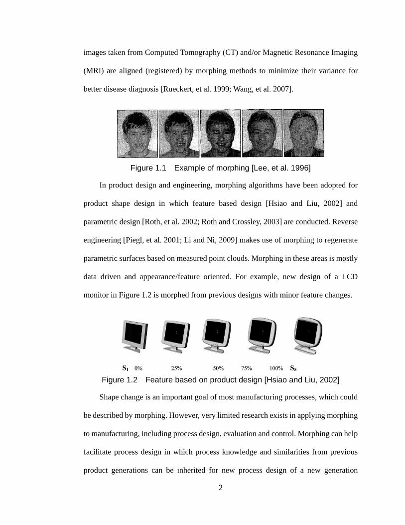
Morphing is one image transformation method describing a complex and seamless
transition of an object from one shape to another. It is widely used in the areas of
computer graphics, filming, medical imaging, etc. In computer graphics and filming,
morphing is an animation technique by which one graphic object is gradually turned
into another using methods such as cross-dissolve, warping, interpolation, etc. Figure
1.1 is an example of face morphing using cross-dissolve which combines the first and
last images with weights. Morphing is also used for video encoding and compression,
where static scenes are connected by morph models [Shum, et al. 2003; Galpin, et al.
2004]. Morphing algorithms are developed and utilized in medical imaging where
2
images taken from Computed Tomography (CT) and/or Magnetic Resonance Imaging
(MRI) are aligned (registered) by morphing methods to minimize their variance for
better disease diagnosis [Rueckert, et al. 1999; Wang, et al. 2007].
Figure 1.1 Example of morphing [Lee, et al. 1996]
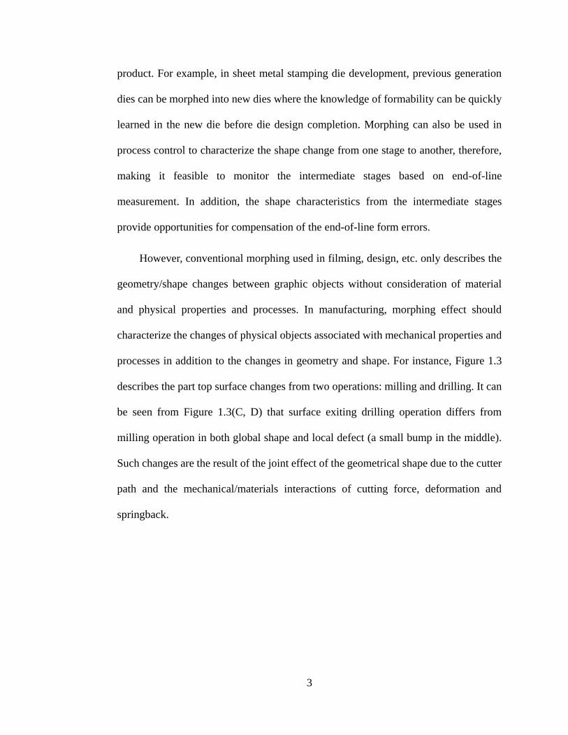
In product design and engineering, morphing algorithms have been adopted for
product shape design in which feature based design [Hsiao and Liu, 2002] and
parametric design [Roth, et al. 2002; Roth and Crossley, 2003] are conducted. Reverse
engineering [Piegl, et al. 2001; Li and Ni, 2009] makes use of morphing to regenerate
parametric surfaces based on measured point clouds. Morphing in these areas is mostly
data driven and appearance/feature oriented. For example, new design of a LCD
monitor in Figure 1.2 is morphed from previous designs with minor feature changes.
Figure 1.2 Feature based on product design [Hsiao and Liu, 2002]
Shape change is an important goal of most manufacturing processes, which could
be described by morphing. However, very limited research exists in applying morphing
to manufacturing, including process design, evaluation and control. Morphing can help
facilitate process design in which process knowledge and similarities from previous
product generations can be inherited for new process design of a new generation
3
product. For example, in sheet metal stamping die development, previous generation
dies can be morphed into new dies where the knowledge of formability can be quickly
learned in the new die before die design completion. Morphing can also be used in
process control to characterize the shape change from one stage to another, therefore,
making it feasible to monitor the intermediate stages based on end-of-line
measurement. In addition, the shape characteristics from the intermediate stages
provide opportunities for compensation of the end-of-line form errors.
However, conventional morphing used in filming, design, etc. only describes the
geometry/shape changes between graphic objects without consideration of material
and physical properties and processes. In manufacturing, morphing effect should
characterize the changes of physical objects associated with mechanical properties and
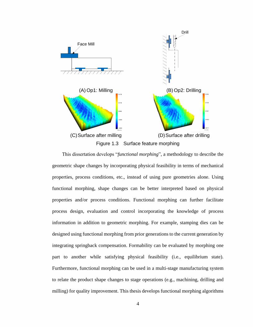
processes in addition to the changes in geometry and shape. For instance, Figure 1.3
describes the part top surface changes from two operations: milling and drilling. It can
be seen from Figure 1.3(C, D) that surface exiting drilling operation differs from
milling operation in both global shape and local defect (a small bump in the middle).
Such changes are the result of the joint effect of the geometrical shape due to the cutter
path and the mechanical/materials interactions of cutting force, deformation and
springback.
4
(A) Op1: Milling (B) Op2: Drilling
(C) Surface after milling (D) Surface after drilling
Figure 1.3 Surface feature morphing
This dissertation develops “functional morphing”, a methodology to describe the
geometric shape changes by incorporating physical feasibility in terms of mechanical
properties, process conditions, etc., instead of using pure geometries alone. Using
functional morphing, shape changes can be better interpreted based on physical
properties and/or process conditions. Functional morphing can further facilitate
process design, evaluation and control incorporating the knowledge of process
information in addition to geometric morphing. For example, stamping dies can be
designed using functional morphing from prior generations to the current generation by
integrating springback compensation. Formability can be evaluated by morphing one
part to another while satisfying physical feasibility (i.e., equilibrium state).
Furthermore, functional morphing can be used in a multi-stage manufacturing system
to relate the product shape changes to stage operations (e.g., machining, drilling and
milling) for quality improvement. This thesis develops functional morphing algorithms
Face Mill
Drill
5
and explores the applications in manufacturing process design, evaluation and control.
1.2. LITERATURE REVIEW
This section conducts a comprehensive review of related literature on morphing
and the research attempts using morphing in manufacturing process development and
control.
1.2.1. Image Transformation
In computer graphics, morphing effects are captured by mathematical
transformation which maps any point on the source object to the corresponding point
on the target object. The most commonly used transformation techniques include affine
transformation and quadratic transformation [Hearn and Baker, 1994], and free-form
deformation (FFD) [Sederberg and Parry, 1986; Coquillart, 1990]. The affine
transformation is usually utilized for rigid body but lacks the degrees of freedom
needed to describe the complex shape changes. Quadratic transformation offers more
but still limited degrees of freedom. FFD are commonly adopted for more complex
shape changes with localized deformation. However, these image transformation
methods and applications are mostly data-oriented and may yield transformations that
are difficult to be interpreted since no physical insights are provided.
Researches were attempted in integrating mechanical attributes into conventional
morphing algorithm. Thin-Plate Spline (TPS) [Bookstein, 1989], which is derived from
minimization of bending energy of a thin plate subjected to key points constraints, is
one such effort. Radial basis functions are introduced to interpolate the intermediate
points besides those key points. In medical imaging research, smoothness function is

6
also integrated into image transformation [Rueckert, et al. 1999; Hill, et al. 2001] so
that a smooth transformation concerning continuity is satisfied. In manufacturing, such
smoothness is not sufficient to accurately characterize the change of shape, for example,
of a non-homogenous density distribution or heterogeneous material. Therefore,
functional morphing in manufacturing will need a more accurate measure of physical
attributes.
1.2.2. Morphing in Process Design, Evaluation and Control
Manufacturing Process Design
Manufacturing process design often involves process selection, process parameter
design, and tooling/fixture design. Process selection and parameter design are
performed by examining the shape and tolerance requirements of individual features,
selecting a process that is capable of meeting the requirements and choosing the
process parameters so as to minimize the effects on performance arising from variation
in manufacture, environment and cumulative damage. This line of research includes
robust parameter design by Feng and Kusiak [1996, 1997, 2000], loss function based
tolerance allocation by Anwarul and Liu[1995], Choi et al. [2000], and Li [2000, 2002],
economic design by Jeang [2002] and multistage process tolerance design [Huang and
Shi, 2003; Ding, et al. 2005]. Efforts have also been made by researchers to address
several parameter issues at the same time. For example, Jeang and Chang [2002]
proposed to concurrently optimize process mean and tolerances. Zhang [1997]
developed simultaneous tolerance analysis and synthesis; Huang and Shi [2003]
developed simultaneous tolerance synthesis via variation propagation modeling.
Among these studies, design of experiment (DOE), response surface model and

7
Taguchi‟s robust parameter design are commonly used methodologies.
In tooling and fixture design, efforts were made to improve the key product
characteristics (KPC) by optimizing choice of fixture and location schemes. Cai et al.
[1997] proposed a variational method for robust fixture configuration design for 3D
rigid parts. Wang and Pelinescu [2001] developed an algorithm for fixture synthesis of
3D workpieces by selecting the positions of the clamps from a collection of locations.
In the design of fixtures for compliant parts, finite element method is used to model and
analyze workpiece behavior [Lee and Haynes, 1987]. Camelio et al. [2004] determined
the optimal fixture location to hold sheet metal parts considering out of plane variation
of fixtures. Cai and Hu [1996] studied the use of the “N-2-1” fixture to provide
additional support for the part and reduce the part‟s deformation. Izquierdo et al. [2009]
introduced robust fixture layout design for multistage manufacturing lines.
Morphing in design area mostly focuses on product design involving appearance
or shape evolutions. Research in product design using morphing can be found in [Hsiao
and Liu, 2002; Roth and Crossley, 2002; Roth, et al. 2003]. In process design,
morphing algorithms have recently been developed to facilitate CAD/CAE processes.
Mesh morphing is integrated into some commercial software such as DynaForm and
HyperMesh to improve development efficiency by quickly changing the finite element
mesh from one product to another. It is also used for multi-objective process
optimization [Liu and Yang, 2007]. Morphing is utilized in stamping die design to
iteratively compensate springback given the simulated springback information [Yin,
2004; Sarraga, 2004].
Process Evaluation

8
There are two major research topics on process evaluation: (1) manufacturability
evaluation to determine whether the designed process is capable of producing the
product, (2) process capability and sensitivity analysis to achieve high repeatability and
low variability. Traditionally, process evaluation followed an experience-based and
trial-and-error procedure. With the introduction of computer graphics and CAD/CAM
systems, numerical approaches have been widely adopted in process evaluation.
Finite element method (FEM) is one of the popular techniques to evaluate the
manufacturability of a given process design for a product [Wang and Tang, 1985; Lyu
and Saitou, 2005; Johansson, 2008; Choi, et al. 2009]. In process capability analysis,
Kazmer and Roser [1999] defined a capability index called „„robustness index‟‟ for
multiple simultaneous quality characteristics. Taguchi‟s Signal-to-Noise S/N ratio
[1986] is one of the commonly used methodologies. These indices depend on variation
input and are computed directly from the output data of KPCs (Key Product
Characteristics). On the other hand, design evaluation based on sensitivity analysis
defines and develops input-independent ratios. One of the characteristics of
sensitivity-based design evaluation is the characterization of product and process into
Key Characteristics (KC). This line of research can be found in [Ceglarek, et al. 1994;
Thornton, 1999] for single operation process and [Ding, 2002] for multi-station
assembly process using state space approach.
Process evaluation using morphing for shape prediction can be found in recent
research papers. Davis et al. [1996] predicted the wafer uniformity given discrete
measurement points using thin-plate spline interpolation. Similar methodologies can
also be found in Mahayotsanun et al. [2007] and Sah and Gao [2009] where TPS is

9
used to predict pressure distribution of the workpiece-tool interface in stamping sheet
metal for process monitoring and control. Combining design and evaluation, Ryken
and Vance [2000] developed a set of tools using virtual reality integrated with free form
deformation and finite element analysis to facilitate the real-time design process of a
tractor lift arm.
Process Monitoring and Control
The research on manufacturing process control focuses on the variation
propagation analysis that investigates the variations accumulated through upstream
stages and their impact on current and downstream stages. This line of research
includes multistage variation propagation modeling [Mantripragada and Whitney,
1999; Jin and Shi, 1999; Djurdjanovic and Ni, 2001; Zhou, et al. 2003; Camelio, et al.
2003], model based process fault diagnosis [Ding, et al. 2002; Zhou, et al. 2004], as
well as process adjustment with programmable toolings [Wang and Huang, 2007;
Zhong, et al. 2009].
In these studies, surface shape are represented utilizing vectorial surface model
[Huang, et al. 2003] or discrete nodes (obtained from CMM scanning) and
corresponding processes are modeled using engineering knowledge such as kinematics
for rigid bodies [Cai, et al. 1996] and finite element analysis for compliant parts
[Camelio, et al. 2003], or by data driven approach [Apley and Shi, 2001; Liu, et al.
2008]. However, research on morphing methodologies in manufacturing process
monitoring and control has not been attempted.

10
1.2.3. Summary of Literature Review
Shape changes are essential in most manufacturing processes. In manufacturing
process design and evaluation, current research still focuses only on one product or
product line. There is a lack of methodologies of using previously existed process
information for process development of evolutionary products. For process control
purpose, existing methodologies study discrete key product characteristics or surface
vectors and have limitations in analyzing complex shape changes involving material
properties and physical processes. Morphing is one promising method to facilitate
process design for new product based on previous knowledge, as well as process
monitoring and control by characterizing the interdependence of manufacturing stages.
Although morphing algorithms have been widely used in computer graphics, filming,
medical imaging, etc, it is rarely utilized in manufacturing process development. One
concern is that the conventional morphing is data-driven and may not fully characterize
a complex physical process that involves material, mechanics, process condition, etc.
Therefore, there exists a need to extend from the geometry morphing to the
aforementioned “functional morphing” and seek the opportunities in facilitating
manufacturing process development and control.
1.3. RESEARCH OBJECTIVES
The objective of this research is to develop functional morphing methodologies
and algorithms and explore the applications in manufacturing process development
including process design, evaluation and control, specifically for the topics of stamping
die development, formability evaluation and process control for multi-stage machining
process. The research tasks include:
11
1) To develop methodologies for morphing based die face design of
evolutionary product between its generations for sheet metal stamping
process;
2) To develop a strain increment method for formability evaluation based on
functional morphing;
3) To develop functional morphing based monitoring and control algorithms
for multi-stage manufacturing process to improve process stability and
reduce variation.
Fulfillment of the objectives will make it feasible to interpret shape changes based
on physical attributes and process conditions, and further facilitate process
development and improvement.
1.4. ORGANIZATION OF DISSERTATION
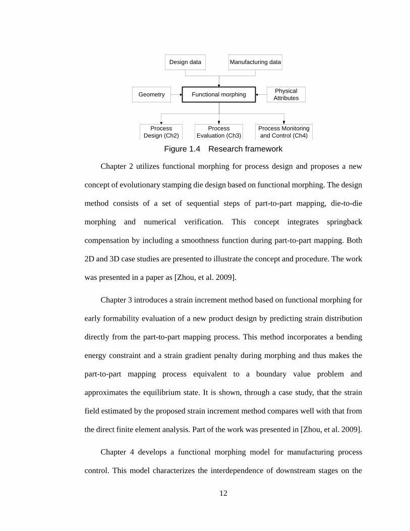
The organization of this dissertation is shown in Figure 1.4. Functional morphing
algorithms are developed by integrating design data (geometric) and manufacturing
information (physical) and then applied onto manufacturing process development
including design evaluation, monitoring and control. This dissertation is presented in a
multiple manuscript format. Chapter 2, 3 and 4 are written as individual research
papers that are partially revised for this dissertation.
12
Figure 1.4 Research framework
Chapter 2 utilizes functional morphing for process design and proposes a new
concept of evolutionary stamping die design based on functional morphing. The design
method consists of a set of sequential steps of part-to-part mapping, die-to-die
morphing and numerical verification. This concept integrates springback
compensation by including a smoothness function during part-to-part mapping. Both
2D and 3D case studies are presented to illustrate the concept and procedure. The work
was presented in a paper as [Zhou, et al. 2009].
Chapter 3 introduces a strain increment method based on functional morphing for
early formability evaluation of a new product design by predicting strain distribution
directly from the part-to-part mapping process. This method incorporates a bending
energy constraint and a strain gradient penalty during morphing and thus makes the
part-to-part mapping process equivalent to a boundary value problem and
approximates the equilibrium state. It is shown, through a case study, that the strain
field estimated by the proposed strain increment method compares well with that from
the direct finite element analysis. Part of the work was presented in [Zhou, et al. 2009].
Chapter 4 develops a functional morphing model for manufacturing process
control. This model characterizes the interdependence of downstream stages on the
Functional morphingGeometryPhysical
Attributes
Process
Design (Ch2)
Process
Evaluation (Ch3)
Process Monitoring
and Control (Ch4)
Design data Manufacturing data

13
surfaces that are generated during upstream stages and explores its applications in
improving variation reduction strategy. It enables multi-scale variation propagation
analysis and intermediate-stage process monitoring and further allows for accurate
inter-stage adjustment that introduces shape deformation upstream to compensate for
the errors downstream. A case study based on a two-stage machining process is
demonstrated to illustrate the monitoring and compensation algorithms. This work will
be published as [Zhou, et al. 2009].
Chapter 5 draws the conclusions and summarizes the original contributions of the
dissertation. Several topics are also proposed for future research.
REFERENCES
Anwarul, M. and Liu, M.C., (1995), “Optimal Manufacturing Tolerance: The Modified
Taguchi Approach”, Proceedings of the Fourth Industrial Engineering
Research Conference, pp. 379-383.
Apley, D. and Shi, J., (2001), “A Factor-Analysis Method for Diagnosing Variability in
Multivariate Manufacturing Processes”, Technometrics, Vol. 43, pp. 84-95.
Bookstein, F.L., (1989), “Principal Warps: Thin-Plate Splines and the Decomposition
of Deformations”, IEEE Transactions on Pattern Analysis and Machine
Intelligence, Vol. 11, pp. 567-585, 1989.
Cai, W. and Hu, S.J., (1996), “Optimal Fixture Configuration Design for Sheet Metal
Assembly With Spring Back”, Transactions of NAMRI/SME, Vol. 23, pp.
229-234
Cai, W., Hu, S.J. and Yuan, J.X., (1997), “A Variational Method of Robust Fixture
Configuration Design for 3-D Workpieces”, ASME Transactions: Journal of
Manufacturing Science and Engineering, Vol. 119 (4), pp. 593-602.
Camelio, J. and Hu, J., Ceglarek, D., (2003), “Modeling Variation Propagation of
Multi-Station Assembly Systems with Compliant Parts”, ASME Transactions:
Journal of Mechanical Design, Vol. 125, pp. 673-681.
Camelio, J., Hu, S.J. and Ceglarek, D., (2004), “Impact of Fixture Design on Sheet
Metal Assembly Variation”, Journal of Manufacturing Systems, Vol. 23 (3), pp.
182-193.
14
Ceglarek, D., Shi, J. and Wu, S.M., (1994), „„A Knowledge-Based Diagnostic
Approach for the Launch of the Auto-Body Assembly Process‟‟, ASME
Transactions: Journal of Engineering for Industry, Vol. 116, pp. 491-499.
Choi, H.G.R., Park, M.H. and Salisbury, E., (2000), “Optimal Tolerance Allocation
with Loss Function”, ASME Transactions: Journal of Manufacturing Science
and Engineering, Vol. 122 (3), pp. 529-535.
Choi, K.S., Liu, W.N., Sun, X., Khaleel, M.A. and Fekete, J.R., (2009), “Influence of
Manufacturing Processes and Microstructures on the Performance and
Manufacturability of Advanced High Strength Steels”, Journal of Engineering
Materials and Technology, Vol.131.
Coquillart, S., (1990), “Extended Free-form Deformation: A Sculpturing Tool for 3D
Geometric Modeling,” ACM SIGGRAPH Computer Graphics, Vol. 24, pp.
187-196.
Davis, J.C., Gyurcsik, R.S., Lu, J.-C. and Hughes-Oliver, J.M., (1996), “A Robust
Metric for Measuring Within-Wafer Uniformity”, IEEE Transactions on
Components, Packaging, and Manufacturing Technology – Part C, Vol. 19, pp.
283-289.
Ding, Y., Ceglarek, D., and Shi, J., (2002), “Design Evaluation of Multi-station
Assembly Processes by Using State Space Approach”, ASME Transactions:
Journal of Mechanical Design, Vol. 124, pp. 408-418.
Ding, Y., Ceglarek, D., and Shi, J., (2002), “Fault Diagnosis of Multistage
Manufacturing Processes by Using State Space Approach”, ASME
Transactions: Journal of Manufacturing Science and Engineering, Vol. 124 (2),
pp. 313-322.
Ding, Y., Jin, J., Ceglarek, D., and Shi, J., (2005), “Process-oriented Tolerancing for
Multi-station Assembly Systems”, IIE Transactions, Vol. 37, pp. 493-508.
Djurdjanovic, D. and Ni, J., (2001), “Linear State Space Modeling of Dimensional
Machining Errors”, Transactions of NAMRI/SME, Vol. 29, pp. 541-548.
Feng, C.X. and Kusiak, A., (1997), “Robust Tolerance Design with the Integer
Programming Approach,” ASME Transactions: Journal of Manufacturing
Science and Engineering, Vol. 119 (44), pp. 603-610.
Feng, C.X. and Kusiak, A., (2000), “Robust Tolerance Design with the Design of
Experiments Approach”, ASME Transactions: Journal of Manufacturing
Science and Engineering, Vol. 122 (3), pp. 520-528.
Galpin, F., Balter, R., Morin, L. and Deguchi, K., (2004), “3D Models Coding and
Morphing for Efficient Video Compression”, Proceedings of the Conference on
Computer Vision and Pattern Recognition, Washington, DC.
15
Hearn, D. and Baker, M.P., (1994), Computer Graphics. 2nd Edn., Prentice Hall.
Hill, D.L.G., Batchelor, P.G., Holden, M. and Hawkes, D.J., (2001), “Medical Image
Registration”, Physics in Medicine and Biology, Vol. 46, pp. R1-R45.
Hsiao, S.W. and Liu, M.C., (2002), “A Morphing Method for Shape Generation and
Image Prediction in Product Design”, Design Studies, Vol. 23 (6), pp. 533-556.
Huang, Q. and Shi, J., (2003), “Simultaneous Tolerance Synthesis through Variation
Propagation Modeling of Multistage Manufacturing Processes”, Transactions
of NAMRI/SME, Vol. 31, pp. 515-522.
Huang, Q., Shi, J. and Yuan, J., (2003), “Part Dimensional Error and its Propagation
Modeling in Multi-Stage Machining Processes,” ASME Transactions: Journal
of Manufacturing Science and Engineering, Vol. 125, pp. 255-262.
Izquierdo, L.E., Hu, S.J., Du, H., Jin, R., Jee, H. and Shi, J., (2009), “Robust Fixture
Layout Design for a Product Family Assembled in a Multistage Reconfigurable
Line”, ASME Transactions: Journal of Manufacturing Science and
Engineering, Vol. 131.
Jeang, A., (2002), “Optimal Parameter and Tolerance Design with a Complete
Inspection Plan”, International Journal of Advanced Manufacturing
Technology, Vol. 20 (2), pp.121-127.
Jeang, A. and Chang, C.L., (2002), “Concurrent Optimization of Parameter and
Tolerance Design via Computer Simulation and Statistical Method”,
International Journal of Advanced Manufacturing Technology, Vol. 19 (6), pp.
432-441.
Jin, J. and Shi, J., (1999), “State Space Modeling of Sheet Metal Assembly for
Dimensional Control”, ASME Transactions: Journal of Manufacturing Science
and Engineering, Vol. 121, pp. 756-762.
Johansson, J., (2008), “Manufacturability Analysis Using Integrated KBE, CAD and
FEM”, Proceedings of the ASME International Design Engineering Technical
Conferences and Computers and Information in Engineering Conference,
DETC 2008, Vol. 5, pp. 191-200.
Kazmer, D. and Roser, C., (1999), „„Evaluation of Product and Process Design
Robustness‟‟, Research in Engineering Design, Vol. 11 (1), pp. 21-30.
Kusiak, A. and Feng, C.X., (1996), “Robust Tolerance Design for Quality”, ASME
Transactions: Journal of Engineering for Industry, Vol. 118 (1), pp.166-169.
Lee, J. and Haynes, L., (1987), “Finite Element Analysis of Flexible Fixturing System”,
ASME Transactions: Journal of Engineering for Industry, Vol. 109 (22), pp.
579-584.

16
Lee, S., Wolberg, G., Chwa, K.Y. and Shin S.Y., (1996), “Image Metamorphosis with
Scattered Feature Constraints”, IEEE Transaction on Visualization and
Computer Graphics, Vol. 2 (4), pp. 337-354.
Li, M.H., (2000), “Quality Loss Function Based Manufacturing Process Setting
Models for Unbalanced Tolerance Design”, International Journal of Advanced
Manufacturing Technology, Vol. 16 (1), pp. 39-45.
Li, M.H., (2002), “Unbalanced Tolerance Design and Manufacturing Setting with
Asymmetrical Linear Loss Function”, International Journal of Advanced
Manufacturing Technology, Vol. 20 (5), pp. 334-340.
Li, Y. and Ni, J., (2009), “Constraints Based Nonrigid Registration for 2D Blade Profile
Reconstruction in Reverse Engineering”, Journal of Computing and
Information Science in Engineering, Vol. 9.
Liu, J., Shi, J. and Hu, S.J., (2008), “Engineering-Driven Factor Analysis for Variation
Sources Identification in Multistage Manufacturing Processes”, ASME
Transactions: Journal of Manufacturing Science and Engineering, Vol. 130 (4),
pp. 041009 1-10.
Liu, W. and Yang, Y., (2007), “Multi-Objective Optimization of an Auto Panel
Drawing Die Face Design by Mesh Morphing”, Computer-Aided Design, Vol.
39, pp. 863-869.
Lyu, N. and Saitou, K., (2005), “Topology Optimization of Multicomponent Beam
Structure via Decomposition-Based Assembly Synthesis”, ASME Transactions:
Journal of Mechanical Design, Vol. 127, pp. 170-183.
Mahayotsanun, N., Cao, J., Peshkin, M., Sah, S., Gao, R. and Wang, C.T., (2007),
“Integrated Sensing System for Stamping Monitoring Control”, Proceedings of
IEEE Sensors 2007 Conference, San Diego, CA, pp. 1376-1379.
Mantripragada, R. and Whitney, D.E., (1999), “Modeling and Controlling Variation
Propagation in Mechanical Assemblies Using State Transition Models”, IEEE
Transactions on Robotics and Automation, Vol. 15, pp. 124-140.
Menassa, R.J. and DeVries, W.R., (1991), “Optimization Methods Applied to Selecting
Support Positions in Fixture Design”, ASME Transactions: Journal of
Engineering for Industry, Vol. 113 (4), pp. 412-418.
Piegl, L.A. and Tiller, W., (2001), “Parameterization for Surface Fitting in Reverse
Engineering”, Computer-Aided Design, Vol. 33 (8), pp. 593-603.
Ryken, M. and Vance, J. M., (2000), “Applying Virtual Reality Techniques to The
Interactive Stress Analysis of a Tractor Lift Arm”, Finite Elements in Analysis
and Design, Vol. 35, pp. 141-155.

17
Roth, B. and Crossley, W.A., (2003), “Application of Optimization Techniques in the
Conceptual Design of Morphing Aircraft”, AIAA's 3rd Annual Aviation
Technology: Integration, and Operations (ATIO), Denver, CO.
Roth, B., Peters, C. and Crossley, W.A., (2002), “Aircraft Sizing with Morphing as an
Independent Variable: Motivation, Strategies, and Investigations”, AIAA Paper
2002-5840, Oct. 2002.
Rueckert, D., Sonoda, L.I., Hayes, C., Hill, D.L.G., Leach, M.O. and Hawkes, D.J.,
(1999), “Nonrigid Registration Using Free-Form Deformations: Application to
Breast MR Images”, IEEE Transactions on Medical Imaging, Vol. 18 (8),
pp.712- 721.
Sah, S. and Gao, R.X., (2009), “Integrated Sensing of Pressure Distribution at The
Workpiece-Tool Interface in Sheet Metal Stamping”, Proceedings of 2009
AMSE Manufacturing Science and Engineering Conference, West Lafayette,
IN, Paper No. MSEC2009-84342.
Sarraga, R., (2004). “Modifying CAD/CAM Surfaces According to Displacements
Prescribed at a Finite Set of Points”, Computer-Aided Design, Vol. 36, pp.
343-349.
Sederberg, T.W. and Parry, S.R., (1986), “Free-form Deformation of Polygonal Data”,
Proceedings of International Electronic Image Week, Nice, France, pp.
633-639.
Shum, H.Y., Sing, B.K. and Chan, S.C., (2003), “Survey of Image-Based
Representations and Compression Techniques”, IEEE Transactions on Circuits
and Systems for Video Technology, Vol. 13 (11), pp.1020-1037.
Taguchi, G., (1986), Introduction to Quality Engineering, Asian Productivity
Organization, Tokyo, Japan.
Thornton, A.C., (1999), „„A Mathematical Framework for the Key Characteristic
Process‟‟, Research in Engineering Design, Vol. 11, pp. 145-157.
Wang, H. and Huang, Q., (2007), “Using Error Equivalence Concept to Automatically
Adjust Discrete Manufacturing Processes for Dimensional Variation
Reduction”, ASME Transactions: Journal of Manufacturing Science and
Engineering, Vol. 129, pp. 644-652.
Wang, M., Hu, H. and Qin, B., (2007), “Non-Rigid Medical Image Registration Using
Optical Flow and Locally-Refined Multilevel Free Form Deformation”,
Nuclear Science Symposium Conference Record, Vol. 6, pp. 4552-4555.
Wang, M.Y. and Pelinescu, D.M., (2001), “Optimizing Fixture Layout in a Point-Set
Domain”, IEEE Transactions on Robotics and Automation, Vol. 17 (3), pp.
312-323.

18
Wang, N.M and Tang, S.C., (1985), Computer Modeling of Sheet Metal Forming
Processes: Theory, Verification and Application, Metallurgical Society.
Yin, Z., Song, J. and Jiang, S., (2004), “A New Strategy for Direct Generation of Tool
Shape from a CAD Model Based on a Meshless Method”, International
Journal of Computer Integrated Manufacturing, Vol. 17, pp. 327-338.
Zhang, G., (1997), “Simultaneous Tolerancing for Design and Manufacturing”,
Advanced Tolerancing Techniques, H. C. Zhang, ed., Wiley, New York,
pp.207-231.
Zhong, J., Liu, J. and Shi, J., (2009), “Predictive Control Considering Model
Uncertainty for Variation Reduction in Multistage Assembly Processes”, IEEE
Transactions on Automation Science and Engineering, Accepted as
TASE-2009-091.
Zhou, L., Hu, S.J. and Stoughton, T.B., (2009), “Formability Assessment in Stamping
Die Face Morphing Using Strain Increment Method”, Proceedings of the ASME
International Manufacturing Science and Engineering Conference (MSEC
2009), West Lafayette, IN.
Zhou, L., Hu, S.J., Stoughton, T.B. and Lin, G., (2009), “Evolutionary Stamping Die
Development Using Morphing Technology”, Transaction of NAMRI/SME, Vol.
37.
Zhou, L., Hu, S.J. and Stoughton, T.B., (2009), “Die Face Morphing with Formability
Assessment”, submitted to ASME Transactions: Journal of Manufacturing
Science and Engineering.
Zhou, L., Wang, H. and Hu, S. J, (2009), “Functional Morphing in Complex
Manufacturing Process and Its Applications in High-Definition Metrology
Based Process Control”, to be submitted to IEEE Transactions on Automation
Science and Engineering.
Zhou, S., Chen, Y. and Shi, J., (2004), “Statistical Estimation and Testing for Variation
Root-Cause Identification of Multistage Manufacturing Processes”, IEEE
Transactions on Robotics and Automation, Vol. 1, pp. 73-83.
Zhou, S., Huang, Q. and Shi, J., (2003) “State Space Modeling for Dimensional
Monitoring of Multistage Machining Process Using Differential Motion
Vector”, IEEE Transactions on Robotics and Automation, Vol. 19, pp.296-309.
19
CHAPTER 2 1
FUNCTIONAL MORPHING BASED EVOLUTIONARY
STAMPING DIE DEVELOPMENT
ABSTRACT
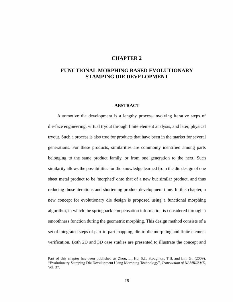
Automotive die development is a lengthy process involving iterative steps of
die-face engineering, virtual tryout through finite element analysis, and later, physical
tryout. Such a process is also true for products that have been in the market for several
generations. For these products, similarities are commonly identified among parts
belonging to the same product family, or from one generation to the next. Such
similarity allows the possibilities for the knowledge learned from the die design of one
sheet metal product to be 'morphed' onto that of a new but similar product, and thus
reducing those iterations and shortening product development time. In this chapter, a
new concept for evolutionary die design is proposed using a functional morphing
algorithm, in which the springback compensation information is considered through a
smoothness function during the geometric morphing. This design method consists of a
set of integrated steps of part-to-part mapping, die-to-die morphing and finite element
verification. Both 2D and 3D case studies are presented to illustrate the concept and
Part of this chapter has been published as Zhou, L., Hu, S.J., Stoughton, T.B. and Lin, G., (2009),
“Evolutionary Stamping Die Development Using Morphing Technology”, Transaction of NAMRI/SME,
Vol. 37.

20
procedure.
2.1. INTRODUCTION
In auto body development, forming is one of the most important manufacturing
processes to achieve streamlined body and stylish appearance. In forming process
development, Die Face Engineering (DFE) is the connection between design and
manufacturing [Okamoto et al. 1988], which is the step for not only the
parameterization from design concept to CAD models, but also the verification of
feasibility that the designed part can be manufactured cost effectively. However, DFE
is a very complicated and time-consuming procedure. Numerous iterations are usually
needed because both the design specifications and the process feasibility (e.g.,
formability and springback) need to be balanced and satisfied. To facilitate and
expedite the DFE process, systematic methodologies and tools need to be developed.
In vehicle families and product generations, similarities can be commonly
identified among parts belonging to the same product family, or from one generation to
the next (e.g. 1997-2003 vs. 2004-2007 or 2008 Chevy Malibu) (Figure 2.1). But, the
current die design approach does not make full use of such similarity and still requires
every step of DFE for each part in the new product generation. This process is not only
expensive but also time consuming.
Figure 2.1 Product family of Chevy Malibu from 1997 to 2008
21
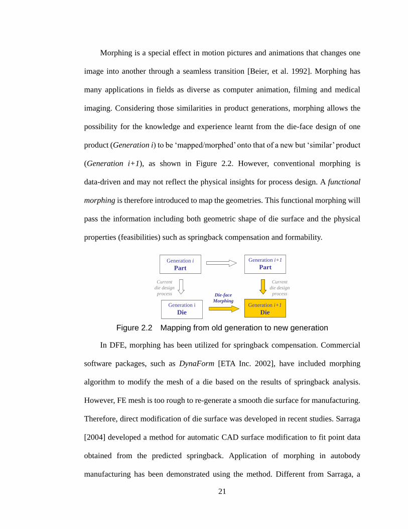
Morphing is a special effect in motion pictures and animations that changes one
image into another through a seamless transition [Beier, et al. 1992]. Morphing has
many applications in fields as diverse as computer animation, filming and medical
imaging. Considering those similarities in product generations, morphing allows the
possibility for the knowledge and experience learnt from the die-face design of one
product (Generation i) to be „mapped/morphed‟ onto that of a new but „similar‟ product
(Generation i+1), as shown in Figure 2.2. However, conventional morphing is
data-driven and may not reflect the physical insights for process design. A functional
morphing is therefore introduced to map the geometries. This functional morphing will
pass the information including both geometric shape of die surface and the physical
properties (feasibilities) such as springback compensation and formability.
Figure 2.2 Mapping from old generation to new generation
In DFE, morphing has been utilized for springback compensation. Commercial
software packages, such as DynaForm [ETA Inc. 2002], have included morphing
algorithm to modify the mesh of a die based on the results of springback analysis.
However, FE mesh is too rough to re-generate a smooth die surface for manufacturing.
Therefore, direct modification of die surface was developed in recent studies. Sarraga
[2004] developed a method for automatic CAD surface modification to fit point data
obtained from the predicted springback. Application of morphing in autobody
manufacturing has been demonstrated using the method. Different from Sarraga, a
Generation i
Part
Generation i
Die
Generation i+1
Part
Die-face
Morphing
Current
die design
process
Current
die design
process
Generation i+1
Die

22
meshless method was introduced for springback simulation by Yin [2004]. This
method is more efficient since it generates the new die surface directly by avoiding the
steps of meshing NURBS surface and separate finite element analysis.
However, very limited work exists in systematic evolutionary die design
incorporating existing part/die information while integrating both geometry and
physical constraints. Hence this chapter proposes a new concept of evolutionary die
design using functional morphing. This design method consists of a set of integrated
steps of part-to-part mapping, die-to-die morphing and finite element verification.
Success of this method will facilitate faster design processes of new products by
reducing iterations in the DFE process between design and manufacturing.
This chapter is organized as follows: Section 2.2 presents a method for die face
morphing described by a sequence of part-to-part mapping, die-to-die morphing and
numerical verification. Part geometry involving trimmed surfaces is also discussed.
Section 2.3 presents a 2D case study of U-shaped channel stamping and a 3D case
study of cup drawing using the proposed method. Section 2.4 summarizes the chapter
with conclusions.
2.2. DIE FACE MORPHING ALGORITHM
Assume that the part geometries from generation i and new generation i+1 are
known (Figure 2.2), denoted as the source and the target geometries. The existing part
and new part are defined by Non-Uniform Rational B-Spline (NURBS) curves/surfaces,
whose control points (CPs) and degrees of freedom (DOF) are both known. The
following die morphing procedures are proposed, as shown in Figure 2.3:

23
(1) A mapping function is obtained by functional morphing algorithm between the
old part geometry and the new part geometry, represented by a set of NURBS
control points. This registration is done by maximizing the correspondence
between the two geometries where the mutual distance between the two
surfaces is minimized.
(2) Using the same mapping function obtained from part-to-part mapping, the old
die geometry, which is also represented by a set of control points, is morphed
onto the new die surface. In this die-to-die morphing, springback information
from the previous generation die, which is reflected in the differences in shape
between the previous part and previous dieface in the part area, is expected to
be carried is expected to be carried into the next generation die.
(3) For verification, forming analysis is conducted using finite element analysis
(FEA) on the new morphed die. The part created by the morphed die is then
compared with the desired part geometry. If the part generated by the morphed
die is not within the design specification, then an iterative approach can be
applied to find the optimal die face.

24
Figure 2.3 Die face morphing concept
2.2.1. Free-Form Representation for Part and Die
In stamping CAD design, the free-form geometries of the part and die are
described by NURBS curves/surfaces [Mortenson 1985; Koivunen et al. 1995]. A
NURBS curve has the mathematical form of,
,
0
( ) ( )n
i p i
i
S R u PP , ,
,
,1
i p i
i p k
j p jj
N wR
N w
(2.1)
where , ( )i pR u is the NURBS basis function of degrees of freedom p, ( 1... )iw i k are
the corresponding weights, ,i pN is the B-Spline basis function, ] [ 10 nPPP P are the
n control points (CP), ] [ 10 muuu U is the knot vector of m knots, and m, n, p satisfy
1pnm .
A NURBS surface (Figure 2.4) is defined as,
Part-to-Part Mapping by Free-
From Deformation
Die-to-Die Morphing by the
same mapping function
Finite Element Verification
Within design
tolerance?
No
Yes
Output new die
geometry
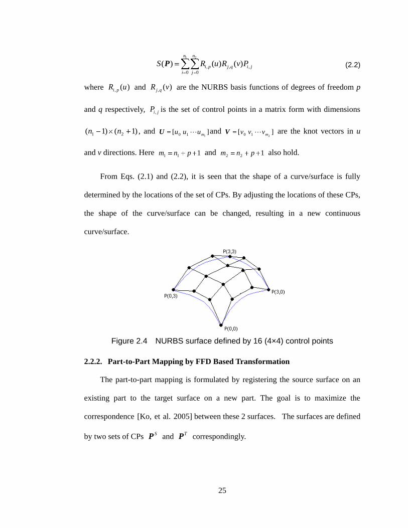
25
1 2
, , ,
0 0
( ) ( ) ( )n n
i p j q i j
i j
S R u R v PP (2.2)
where , ( )i pR u and , ( )j qR v are the NURBS basis functions of degrees of freedom p
and q respectively, jiP , is the set of control points in a matrix form with dimensions
)1()1( 21 nn , and ] [110 muuu U and ] [
210 mvvv V are the knot vectors in u
and v directions. Here 111 pnm and 122 pnm also hold.
From Eqs. (2.1) and (2.2), it is seen that the shape of a curve/surface is fully
determined by the locations of the set of CPs. By adjusting the locations of these CPs,
the shape of the curve/surface can be changed, resulting in a new continuous
curve/surface.
Figure 2.4 NURBS surface defined by 16 (4×4) control points
2.2.2. Part-to-Part Mapping by FFD Based Transformation
The part-to-part mapping is formulated by registering the source surface on an
existing part to the target surface on a new part. The goal is to maximize the
correspondence [Ko, et al. 2005] between these 2 surfaces. The surfaces are defined
by two sets of CPs S
P and T
P correspondingly.

26
1
1 1 1
11 1
1
S S
m
S
S S
n n m
P P
P P
P
2
2 2 2
11 1
1
T T
m
T
T T
n n m
P P
P P
P (2.3)
This correspondence is usually measured using the general distance 1g between
the two surfaces, defined as,
2
1( , )S T S Tg S T SP P P P (2.4)
where TS P is the target surface, )(T is the transformation function on the CP set,
and SS T P is the surface defined by the transformed CP set S
P . Maximizing the
correspondence is equivalent to finding a transformation function )(T to minimize
the general distance ),(1
TSg PP . This transformation function is also referred as a
part-to-part mapping function.
Cubic Free-Form Deformation (FFD) [Rueckert, et al. 1999] is selected as the
transformation method since it is commonly used for localized geometry
transformation in 3D space. The FFD is defined by a tensor-product of uniform cubic
B-Spline blending functions in the form of
3 3 3
, ,
0 0 0
( , , ) ( ) ( ) ( )i j k i j k
i j k
T x y z B u B v B w (2.5)
where, u, v, w are localized coordinates and B is the uniform cubic B-spline function.
u x x
v y y
w z z
, and (2.6)

27
3 2
0
3 2
1
3 2
2
3
3
( ) ( 3 3 1) / 6
( ) (3 6 4) / 6
( ) ( 3 3 1) / 6
( ) / 6
B t t t t
B t t t
B t t t t
B t t
Figure 2.5 Free form deformation: (x,y,z) is the original point, (X,Y,Z) is the new point after FFD
The FFD transformation in Figure 2.5 defines a mapping T: (x,y,z) (X,Y,Z)
where (x,y,z) is from the source space VS, and (X,Y,Z) is from the target space VT. Φ is
the set of lattice points (LP) in R3 which define the space, i.e., the mesh grids.
Let T(0)
denote an identity mapping from (x,y,z) to (x,y,z), i.e.,
3 3 3(0) (0)
, ,
0 0 0
( , , ) ( ) ( ) ( )i j k i j k
i j k
x
y T x y z B u B v B w
z
(2.7)
where kji ,,)0( can be regarded as the set of LPs which defines the original space and
)0(T is the set of CPs defining the source surface. Let T be the increment of the set
of CP while Φ be the increment of set of LP during transformation which satisfies
)0(ΦΦΦ and
TTzyxT )0(),,(
3 3 3 3 3 3(0)
, , , , , ,
0 0 0 0 0 0
( ) ( ) ( ) ( ) ( ) ( )i j k i j k i j k i j k i j k
i j k i j k
B u B v B w B u B v B w
(2.8)
Combining Eqs (2.7) and (2.8), it is seen that the difference between original CPs
VS
(x,y,z)(X,Y,Z)
VT
(X,Y,Z)

28
and new CPs is fully determined by the movement of the corresponding lattice points
Φ .
3 3 3
, ,
0 0 0
( , , ) ( ) ( ) ( )i j k i j k
i j k
T x y z B u B v B w (2.9)
In solving the part-to-part mapping, (x,y,z) is known as CP set S
P and (X,Y,Z) is
known as CP set SP~
, which contains the optimal locations of the CPs of the source
object after achieving the maximum correspondence to the target object. Therefore,
(0) ( , , )S T x y zP
and ( , , )S S T x y zP P (2.10)
From Eqs (2.4), (2.9) and (2.10), the objective 1g is a function of kji ,,, the
movement of the LP set. Therefore, , ,i j k
defines the mapping between the existing
part surface and the new part surface.
FFD based functional morphing for registration
The mathematical goal of the registration is to find a mapping function by moving
the lattice points kji ,, to warp the space VS to the space VT, so that the general
distance between the transformed source object and the target object is minimized. The
optimization problem can be formulated as,
2
1
1
( , )
.
( , )
S T S T
S T
g P P S T S
g
Min
s.t
P P
P P
(2.11)
where Φ is the optimization variable and is the maximum registration error. The
optimal locations of CPs SP~
are obtained by minimizing the general distance 1g
between the transformed source object and the target object.
29
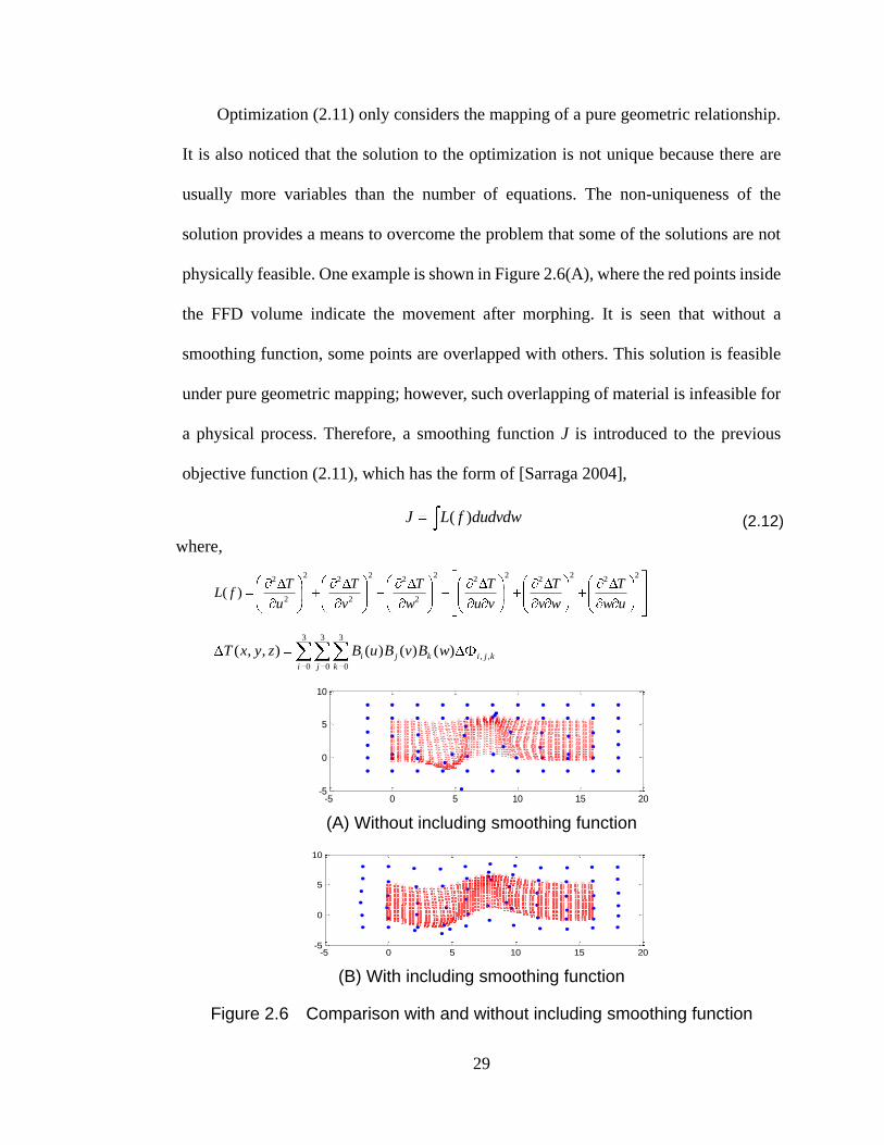
Optimization (2.11) only considers the mapping of a pure geometric relationship.
It is also noticed that the solution to the optimization is not unique because there are
usually more variables than the number of equations. The non-uniqueness of the
solution provides a means to overcome the problem that some of the solutions are not
physically feasible. One example is shown in Figure 2.6(A), where the red points inside
the FFD volume indicate the movement after morphing. It is seen that without a
smoothing function, some points are overlapped with others. This solution is feasible
under pure geometric mapping; however, such overlapping of material is infeasible for
a physical process. Therefore, a smoothing function J is introduced to the previous
objective function (2.11), which has the form of [Sarraga 2004],
( )J L f dudvdw
where,
2 2 2 2 2 22 2 2 2 2 2
2 2 2( )
T T T T T TL f
u v w u v v w w u
3 3 3
, ,
0 0 0
( , , ) ( ) ( ) ( )i j k i j k
i j k
T x y z B u B v B w
(2.12)
(A) Without including smoothing function
(B) With including smoothing function
Figure 2.6 Comparison with and without including smoothing function
-5 0 5 10 15 20-5
0
5
10
0 2 4 6 8 10 12 14 160
5
10
0
1
2
-5 0 5 10 15 20-5
0
5
10
0 2 4 6 8 10 12 14 160
5
10
0
0.5
1
1.5

30
Figure 2.6(B) shows the deformation with the smoothing function from the same
objective function. A smoother morphing result is given by including such a function.
Figure 2.6(B) indicates that inside the FFD volume, the material near the object to be
registered will move in the similar direction, resulting in a smooth deformation. In the
stamping die development, the die surface deviates from part surface for springback
compensation. If the parts from 2 generations are similar in terms of strain path during
stamping, by applying the functional morphing of combined geometric mapping and
smoothness, this springback information will be carried from the prior generation die
into the new generation.
Combining Eqs. (2.11) and (2.12), a final optimization problem (2.13) is defined,
1
2
(1 ) ( , )
(1 ) ( )
S T
S T
g P P J
S T P S P L f dudvdw
Min
s.t.
),(1
TSg PP
where,
1 2
, , ,
0 0
3 3 3(0)
, , , ,
0 0 0
3 3 3(0) (0)
, ,
0 0 0
2 2 22 2 2 2
2 2 2
( ) ( ) ( )
( , , ) ( ) ( ) ( )
( , , ) ( ) ( ) ( )
( )
n n
i p j q i j
i j
i j k i j k i j k
i j k
S
i j k i j k
i j k
S N u N v P
T x y z B u B v B w
T x y z B u B v B w
T T T TL f
u v w
P
P
2 2 22 2T T
u v v w w u
(2.13)
In this optimization problem, is a weight valued between 0 and 1, representing a

31
trade-off between the correspondence and the morphing smoothness. Since Eq. (2.13)
is a non-linear optimization problem, an iterative numerical method is applied to
solving the problem.
2.2.3. Die-to-Die Morphing
The mapping function between the part surfaces is then used to generate the new
die surface given an existing, generation i, die. Such a function, obtained by solving
Φ in the optimization problem (2.13), is then applied on the geometry of the existing
die surface, which is also defined by a set of CPs, to generate the new die surface.
Morphing of the die surface is done through free form deformation,
3 3 3(0)
, , , ,
0 0 0
( , , ) ( ) ( ) ( )d d d i d j d k d i j k i j k
i j k
T x y z B u B v B w (2.14)
where (ud, vd, wd) are local coordinates corresponding to the global coordinates (xd, yd,
zd) of the control points from the existing die face, (0)
, ,i j k are the LPs to define the
original FFD volume space while , ,i j k is the increment of LPs to define the
part-to-part mapping. Finally, the new die surface generated by Eq. (2.14) is verified
using finite element method and the result is compared with the desired part shape.
2.2.4. Consideration on Trimmed Surfaces
More complex product shape (surfaces) cannot be represented by NURBS
surfaces with their control points defined in a matrix form (Eq. (2.3)). In such a case,
trimmed surface is used which consists of both a NURBS surface and closed loop
boundaries. Trimmed surface is commonly used for the representations of feature
edges and the connection between multiple surface patches. For example, the green

32
surface shown in Figure 2.7 has a feature edge on the top right corner. It is trimmed
from the original NURBS surface (blue surface) by a close-loop boundary (red lines).
Figure 2.7 Sample of trimmed surface
In the Initial Graphics Exchange Specification (IGES) [IGES/PDES Organization,
1997], boundaries lines/curves are defined by a set of 2D B-spline curves in local
coordinate system between 0 and 1. For example, a regular B-spline surface consists of
4 straight lines with coordinates (0,0)-(1,0), (1,0)-(1,1), (1,1)-(0,1) and (0,1)-(0,0). The
sample surface shown above has the boundary lines plotted in Figure 2.8. It is seen that
there are 5 boundary lines connected together to trim the original NURBS surface.
Figure 2.8 Boundary lines of sample trimmed surface
In die face morphing for trimmed surfaces, the mapping function needs to include
Feature edge
Orig. surface
Trimmed surface
0 0.2 0.4 0.6 0.8 1
0
0.2
0.4
0.6
0.8
1

33
the boundaries, so that in the die-to-die morphing step, the morphed new die surface
can also be trimmed to produce the desired part. Therefore, the following part-to-part
mapping including boundary mapping is proposed:
1) Solve part-to-part mapping from Eq.(2.13) using the untrimmed source
surface to register with target surface. This step is the same as the mapping
of untrimmed surfaces.
2) Project the boundary points of target (points cloud) onto the transformed
source surface and cluster them into groups. The number of groups equals
to the number of boundary lines/curves. In this step, statistical clustering
techniques can be used to group these boundary points on the transformed
source surface, e.g., K-Means [Johnson and Wichern, 2001] is one of the
efficient methods to cluster the spatial distributed points.
3) Fit each group of boundary points to a spline in the local coordinate to
obtain the boundary curves. These boundary curves can be further used to
trim the morphed dies accordingly and generate new die surface.
A case study utilizing the proposed method will be demonstrated in Section 2.3.3.
2.3. CASE STUDY
2.3.1. 2D Study on Stamping U-shaped Channel
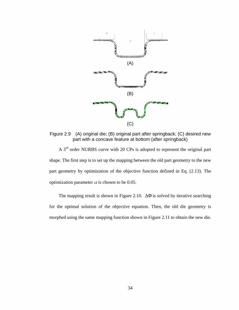
A stamping process for a U-shaped channel is shown in Figure 2.9 (A, B) with the
original part and die geometries both known. A concave feature is added onto the part
shape (Figure 2.9 (C)). The proposed morphing method is applied to generate a new die
shape for the new part.
34
(A)
(B)
(C)
Figure 2.9 (A) original die; (B) original part after springback; (C) desired new part with a concave feature at bottom (after springback)
A 3rd
order NURBS curve with 20 CPs is adopted to represent the original part
shape. The first step is to set up the mapping between the old part geometry to the new
part geometry by optimization of the objective function defined in Eq. (2.13). The
optimization parameter is chosen to be 0.05.
The mapping result is shown in Figure 2.10. is solved by iterative searching
for the optimal solution of the objective equation. Then, the old die geometry is
morphed using the same mapping function shown in Figure 2.11 to obtain the new die.

35
(A) Initial state
(B) After Mapping
Figure 2.10 Part-to-part mapping (dots: lattice points, cross: control points of morphed original part, circle: desired new part, line: NURBS curve generated
from the control points)
Figure 2.11 Die-to-die morphing (dots: lattice points, Cross: control points of the morphed die, solid line: Die surface, dashed line: desired part surface)
For the verification of the new die surface generated by the procedure, an FE
analysis is performed by extracting and meshing the die geometry. The simulation
environment is ABAQUS 6.8 with Explicit and Standard solver [ABAQUS Inc. 2008].
The material model is elastic/plastic using aluminum alloy AA6111-T4. The material
-10 0 10 20 30 40 50 60-4
-2
0
2
4
6
8
10
12
14
16
-10 0 10 20 30 40 50 60-4
0
4
8
12
16
-10 0 10 20 30 40 50 60-4
-2
0
2
4
6
8
10
12
14
16
-10 0 10 20 30 40 50 60-4
0
4
8
12
16
-10 0 10 20 30 40 50 60
0
5
10
15
Desired part surface
Old die surface
Morphed die surface
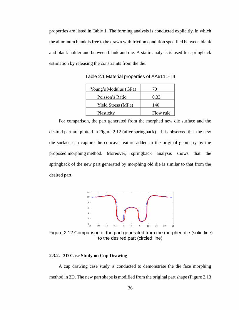
36
properties are listed in Table 1. The forming analysis is conducted explicitly, in which
the aluminum blank is free to be drawn with friction condition specified between blank
and blank holder and between blank and die. A static analysis is used for springback
estimation by releasing the constraints from the die.
Table 2.1 Material properties of AA6111-T4
Young‟s Modulus (GPa) 70
Poisson‟s Ratio 0.33
Yield Stress (MPa) 140
Plasticity Flow rule
For comparison, the part generated from the morphed new die surface and the
desired part are plotted in Figure 2.12 (after springback). It is observed that the new
die surface can capture the concave feature added to the original geometry by the
proposed morphing method. Moreover, springback analysis shows that the
springback of the new part generated by morphing old die is similar to that from the
desired part.
Figure 2.12 Comparison of the part generated from the morphed die (solid line) to the desired part (circled line)
2.3.2. 3D Case Study on Cup Drawing
A cup drawing case study is conducted to demonstrate the die face morphing
method in 3D. The new part shape is modified from the original part shape (Figure 2.13
0 5 10 15 20 25 30 35 40 45 500
2
4
6
8
10
12
-250
-20 -15 -10 -5 0 5 10 15 20 25
2
4
6
8
10
12
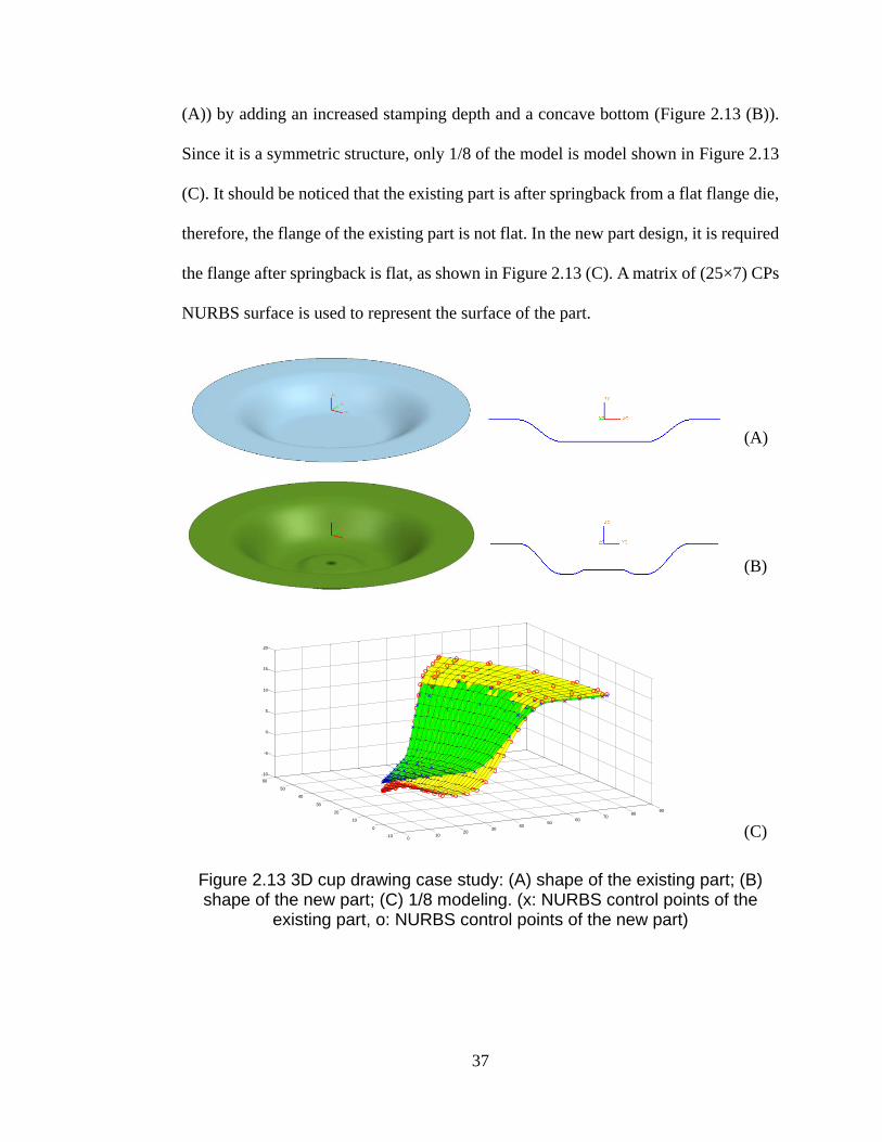
37
(A)) by adding an increased stamping depth and a concave bottom (Figure 2.13 (B)).
Since it is a symmetric structure, only 1/8 of the model is model shown in Figure 2.13
(C). It should be noticed that the existing part is after springback from a flat flange die,
therefore, the flange of the existing part is not flat. In the new part design, it is required
the flange after springback is flat, as shown in Figure 2.13 (C). A matrix of (25×7) CPs
NURBS surface is used to represent the surface of the part.
(A)
(B)
(C)
Figure 2.13 3D cup drawing case study: (A) shape of the existing part; (B) shape of the new part; (C) 1/8 modeling. (x: NURBS control points of the
existing part, o: NURBS control points of the new part)
010
2030
4050
6070
8090
-10
0
10
20
30
40
50
60
-10
-5
0
5
10
15
20
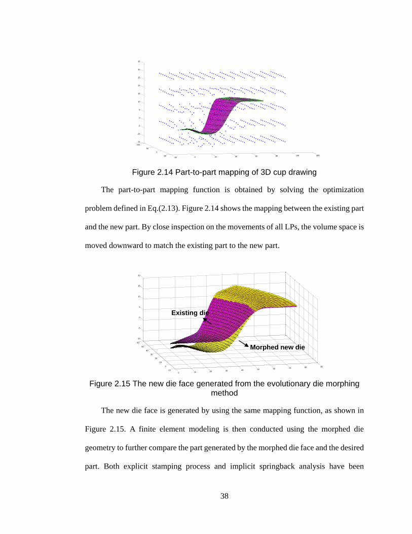
38
Figure 2.14 Part-to-part mapping of 3D cup drawing
The part-to-part mapping function is obtained by solving the optimization
problem defined in Eq.(2.13). Figure 2.14 shows the mapping between the existing part
and the new part. By close inspection on the movements of all LPs, the volume space is
moved downward to match the existing part to the new part.
Figure 2.15 The new die face generated from the evolutionary die morphing method
The new die face is generated by using the same mapping function, as shown in
Figure 2.15. A finite element modeling is then conducted using the morphed die
geometry to further compare the part generated by the morphed die face and the desired
part. Both explicit stamping process and implicit springback analysis have been
-20 0 20 40 60 80 100 120-50
0
50
100
-15
-10
-5
0
5
10
15
20
25
30
35
0 10 20 30 40 50 60 70 80 90
-10
0
10
20
30
40
50
60
-10
-5
0
5
10
15
20
Morphed new die
Existing die

39
performed. Figure 2.16 shows the comparison of the nodes from FEA results and the
surface of the desired part. It is seen that the part generated by the morphed die captures
both features (increased draw depth and concave bottom) added to the original part and
the springback in terms of the flange shape, where the new part has a flat flange as
desired.
Figure 2.16 Comparison of the part generated by the morphed die (point cloud) and the desired part (surface)
2.3.3. Mapping of Trimmed Surface
One challenge proposed in Section 2.2.4 is to deal with trimmed surfaces, in
which part-to-part mapping function will consist of 2 parts: NURBS surface mapping
and boundary mapping. A similar cup drawing case study is shown in Figure 2.17 with
a hole in the middle, in which the hole is trimmed from the original NURBS surface
(only a 1/8 of the surface is shown). The new surface has both increased draw depth
and hole diameter as shown in Figure 2.17(B).
0 10 20 30 40 50 60 70 80 90-20
0
20
40
60
-25
-20
-15
-10
-5
0
0 10 20 30 40 50 60 70 80 90-1000100-25
-20
-15
-10
-5
0

40
(A) old part surface (B) new part surface
Figure 2.17 Case study of trimmed surfaces mapping
Part-to-part mapping function starts from registering the original NURBS surface
of the old part to the new part. The original surface of the existing part is a full cup
without the hole in the middle (Figure 2.18(A)). After registration, only the trimmed
part areas are matched between old and new parts, while the tip area which is trimmed
from the old part surface deforms in the way to improve the smoothness (Figure
2.18(B)).
(A) before part-to-part mapping (surface: untrimmed existing part; circle: new
part surface; cross: control points to be mapped)
(B) after part-to-part mapping (surface: untrimmed existing part; circle: new
part surface; cross: control points to be mapped)
Figure 2.18 Part-to-part mapping for trimmed surfaces
-10 0 10 20 30 40 50 60 70 -200
2040
6080
100-10
-5
0
5
10
15
20
25
30
RED SOLID: Old Part
BLUE DASH: Old Die
GREEN CIR: New Part
-20
0
20
40
60
80-20 0 20 40 60 80 100 120
-15
-10
-5
0
5
10
15
20
25
30
35
02040 1020304050607080
0
5
10
15

41
Clustering method, e.g., K-Means, is utilized to group the boundary nodes. The
number of groups is determined by maximum Silhouette value. Result from K-Means
analysis shown in Figure 2.19 indicates that there are 5 groups, although 2 groups are
suggested on the left border. The boundary points in each group are then fitted into a
B-spline curve.
Figure 2.19 Boundary groups by K-Means
Finally, the new die surface is morphed using the same mapping function from the
old die surface and then trimmed by the fitted boundaries, as shown in Figure 2.20.
Figure 2.20 Die face morphing for trimmed surface
0.2 0.3 0.4 0.5 0.6 0.7 0.8 0.9 1
0
0.2
0.4
0.6
0.8
1
-20-10
010
2030
4050
6070 0
20
40
60
80-10
-5
0
5
10
15
20
25
Morphed new die
Old die

42
2.4. CONCLUSION
A new concept using functional morphing for evolutionary die development has
been proposed using three sequential steps: part-to-part mapping between the existing
part and the new part, die-to-die morphing using the same parts mapping function, and
finite element verification. The following conclusions are drawn:
1) A part-to-part mapping function is established between the part surfaces
from two generations by solving the optimization problem (2.13) based on
functional morphing. This functional morphing allows geometric mapping
with physical feasibility, in which the smoothness function helps inherit
the springback compensation from previous generation die to the new
generation.
2) Methodology for trimmed surfaces morphing is proposed by including a
mapping function of original NURBS surfaces and a boundary mapping.
Statistical clustering method, e.g. K-Means, can be used to group
boundary points to fit B-spline boundary curves.
3) Both 2D and 3D case studies show that, the feature change in the new part
can be captured by the part generated by the morphed die using the same
part-to-part mapping function. Springback is also found similar to the
desired part.
REFERENCES
ABAQUS Inc. (2008). ABAQUS User's Manual.
Beier, T. and Shawn, N., (1992), “Feature-Based Image Metamorphosis”, Computer
Graphics, Vol. 26 (2), pp. 36-42.

43
ETA Inc., (2002), Dynaform-PC User's Manual, Engineering Technology Associates,
Inc.
IGES/PDES Organization, (1997), “Initial Graphics Exchange Specification IGES 5.3”,
U.S. Product Data Association.
Johnson, R. A. and Wichern, D.W., (2001), “Applied Multivariate Statistical Analysis”,
5th Edn., Prentice Hall, New York.
Ko, K., Maekawa and T., Patrikalakis, N., (2005), “Algorithms for Optimal Partial
Matching of Free-Form Objects with Scaling Effects”, Graphical Models, Vol.
67, pp. 120-148.
Koivunen, V. and Bajcsy, R., (1995). “Spline Representations in 3-D Vision”,
Proceedings of International NSF-ARPA Workshop on Object Representation in
Computer Vision, pp. 177-190.
Mortenson, M., (1985), Geometric modeling. John Wiley & Sons, Inc., New York.
Okamoto, I., Takahashi, A., Sugiura, H., Yamada, N. and Mori, T., (1988). “Computer
Aided Design and Evaluation System for Stamping Dies at Toyota”, SAE
Publication: Advances and Trends in Automotive Sheet Steel Stamping, Vol.
206, pp. 79-89.
Rueckert, D., Sonoda, L., Hayes, C., Hill, D., Leach, M. and Hawkes, D., (1999),
“Nonrigid Registration Using Free-Form Deformations: Application to Breast
MR Images”, IEEE Transactions on Medical Imaging, Vol. 18, pp. 712-721.
Sarraga, R., (2004). “Modifying CAD/CAM Surfaces According to Displacements
Prescribed at a Finite Set of Points”, Computer Aided Design , Vol. 36, pp.
343-349.
Yin, Z., Song, J. and Jiang, S., (2004), “A New Strategy for Direct Generation of Tool
Shape from a CAD Model Based on a Meshless Method”, International
Journal of Computer Integrated Manufacturing , Vol. 17, pp. 327-338.

44
CHAPTER 3 2
FUNCTIONAL MORPHING BASED FORMABILITY
ASSESSMENT IN STAMPING DIE FACE MORPHING USING
STRAIN INCREMENT METHOD
ABSTRACT
A strain increment method is proposed for early formability assessment in die face
engineering by predicting the strain distribution directly from the part-to-part mapping
process based on functional morphing. This method consists of mapping the finite
element mesh to the geometry of an existing part, solving the part-to-part mapping
relation by functional morphing integrating a bending energy and strain gradient
penalty functions, and extracting strain increment from the part-to-part mapping
related displacement field. Case studies show that the strain field obtained using the
proposed strain increment method compares well with that from the finite element
analysis. Since this method does not require knowledge of the new die surface, such
formability assessment can serve as an early manufacturing feasibility analysis on the
new part design.
Contents of this chapter have been published as Zhou, L., Hu, S.J. and Stoughton, T.B., (2009),
“Formability Assessment in Stamping Die Face Morphing Using Strain Increment Method”,
Proceedings of the ASME International Manufacturing Science and Engineering Conference (MSEC
2009), West Lafayette, IN. and submitted to ASME Transactions: Journal of Manufacturing Science and
Engineering under Zhou, L., Hu, S.J. and Stoughton, T.B., (2009), “Die Face Morphing with Formability
Assessment”.
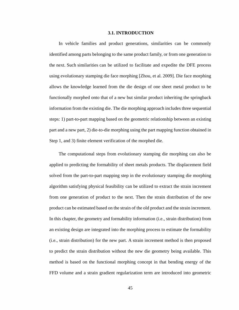
45
3.1. INTRODUCTION
In vehicle families and product generations, similarities can be commonly
identified among parts belonging to the same product family, or from one generation to
the next. Such similarities can be utilized to facilitate and expedite the DFE process
using evolutionary stamping die face morphing [Zhou, et al. 2009]. Die face morphing
allows the knowledge learned from the die design of one sheet metal product to be
functionally morphed onto that of a new but similar product inheriting the springback
information from the existing die. The die morphing approach includes three sequential
steps: 1) part-to-part mapping based on the geometric relationship between an existing
part and a new part, 2) die-to-die morphing using the part mapping function obtained in
Step 1, and 3) finite element verification of the morphed die.
The computational steps from evolutionary stamping die morphing can also be
applied to predicting the formability of sheet metals products. The displacement field
solved from the part-to-part mapping step in the evolutionary stamping die morphing
algorithm satisfying physical feasibility can be utilized to extract the strain increment
from one generation of product to the next. Then the strain distribution of the new
product can be estimated based on the strain of the old product and the strain increment.
In this chapter, the geometry and formability information (i.e., strain distribution) from
an existing design are integrated into the morphing process to estimate the formability
(i.e., strain distribution) for the new part. A strain increment method is then proposed
to predict the strain distribution without the new die geometry being available. This
method is based on the functional morphing concept in that bending energy of the
FFD volume and a strain gradient regularization term are introduced into geometric
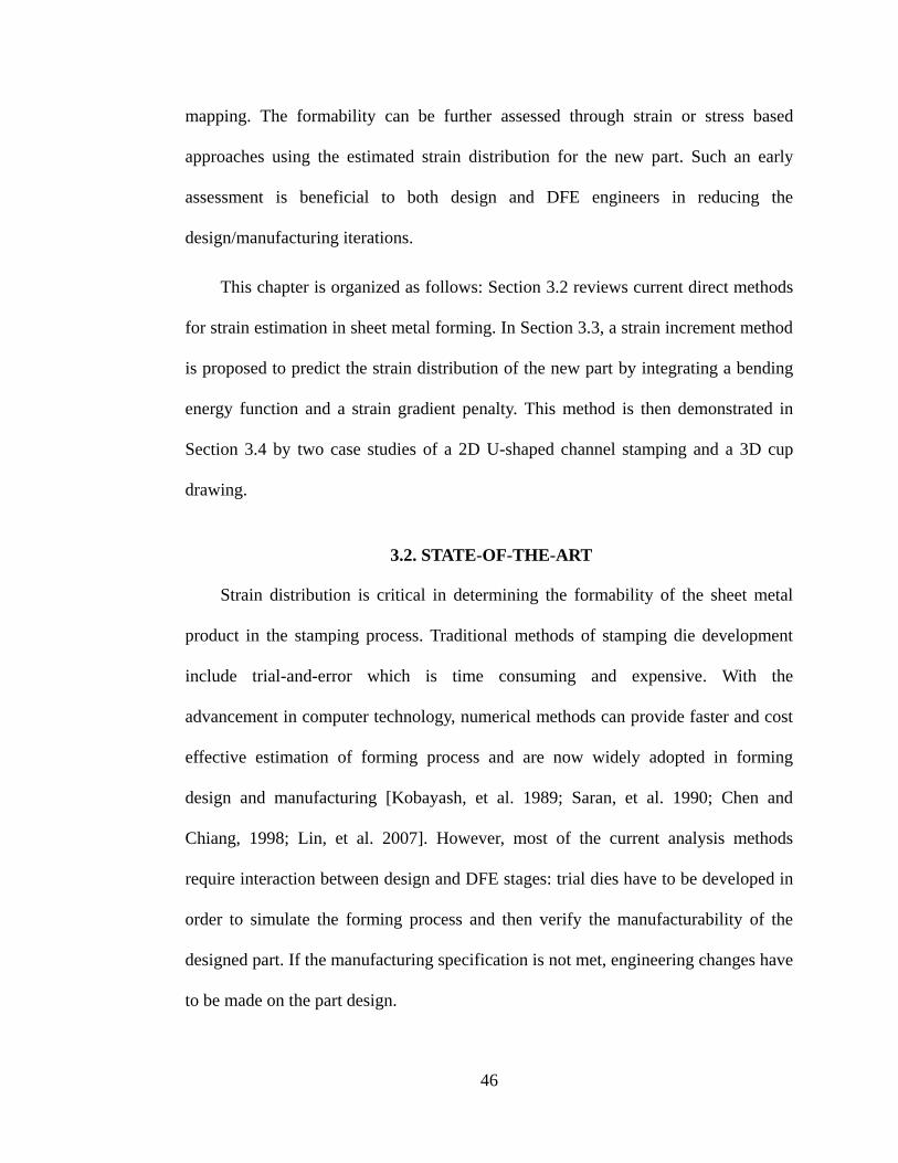
46
mapping. The formability can be further assessed through strain or stress based
approaches using the estimated strain distribution for the new part. Such an early
assessment is beneficial to both design and DFE engineers in reducing the
design/manufacturing iterations.
This chapter is organized as follows: Section 3.2 reviews current direct methods
for strain estimation in sheet metal forming. In Section 3.3, a strain increment method
is proposed to predict the strain distribution of the new part by integrating a bending
energy function and a strain gradient penalty. This method is then demonstrated in
Section 3.4 by two case studies of a 2D U-shaped channel stamping and a 3D cup
drawing.
3.2. STATE-OF-THE-ART
Strain distribution is critical in determining the formability of the sheet metal
product in the stamping process. Traditional methods of stamping die development
include trial-and-error which is time consuming and expensive. With the
advancement in computer technology, numerical methods can provide faster and cost
effective estimation of forming process and are now widely adopted in forming
design and manufacturing [Kobayash, et al. 1989; Saran, et al. 1990; Chen and
Chiang, 1998; Lin, et al. 2007]. However, most of the current analysis methods
require interaction between design and DFE stages: trial dies have to be developed in
order to simulate the forming process and then verify the manufacturability of the
designed part. If the manufacturing specification is not met, engineering changes have
to be made on the part design.
47
In order to reduce the iteration between design and DFE, some direct prediction
methods have been developed to predict the strain distribution directly from part
design. Such methods include ideal forming theory and inverse approach (one-step
solution). The ideal forming theory [Chung and Richmond, 1992, 1994; Chung, et al.
1997] is developed based on the principle of extremum work. In this approach, each
individual material element is locally prescribed to deform in a minimum work path
and the ideal global process is then defined as the one having optimal global plastic
work in a final shape. The inverse approach [Guo, et al. 1990, 2000; Naceur, et al.
2004] is based on the principle of virtual work. It discretizes the part surface by
triangular facet shell elements and computes the inverse deformation tensor to estimate
the large logarithmic strain and predict the initial blank shape. Applications using both
methods have been successfully demonstrated [Sabourin, et al. 2004; Lan, et al. 2005;
Ryou, et al. 2005].
For the design of evolutionary products, both direct methods are capable of
estimating the strain or formability at the design stage without DFE. However, both
methods require generating new finite element mesh once the part design is changed.
Considering the geometric similarity of sheet metal products within the same product
family or in multiple generations, more efficient algorithm can be developed if such
similarity information is utilized. With the implementation of geometric modeling
such as morphing on product design [Hong, et al. 2006; Chen, et al. 2003], morphing
methodology has shown great potential in evolutionary stamping die development.
An evolutionary die face morphing concept was recently developed using functional
morphing [Zhou, et al. 2009] for the stamping process development of metal products

48
from the same product family or different product generations. This functional
morphing algorithm maps geometries between part geometries considering
springback compensation. Based on this morphing algorithm, methodologies for
strain estimation of the similar parts from the same product families is to be
developed in this chapter.
3.3. THE STRAIN INCREMENT METHOD
3.3.1. Geometric Mapping by Free-Form Deformation
The part-to-part mapping procedure as proposed by Zhou, et al. [2009] is briefly
reviewed here. Assume that the part geometries from an existing generation, i, and a
new generation, i+1, are known. The existing part and new part are defined by
Non-Uniform Rational B-Spline (NURBS) curves/surfaces whose control points (CPs)
and degrees of freedom (DOF) are both known. A mapping function, denoted as
part-to-part mapping, is obtained by registration between the existing part geometry
and the new part geometry. This mapping function, defined by the movement ( ) of
Free-form deformation (FFD) [Sederberg and Parry, 1986] lattice points, is solved by
introducing an optimization problem as below:
2
1
1
( , )
.
( , )
S T S T
S T
g P P S T S
g
Min
s.t
P P
P P
(3.1)
where S
P and T
P are B-spline control points matrices of part surfaces from previous
and current generations with dimension of 1 2( 1) ( 1)
S Sn n and 1 2
( 1) ( 1)T T
n n
correspondingly. S is B-spline surface definition in Eq. (2.2). 1g is the general
distance (mutual distance) of the two B-spline surfaces. And is the maximum
49
registration error. The mathematical goal of the registration is to find a mapping
function by moving the lattice points i, j,kΔΦ to warp the FFD volume space VS to the
volume space VT, so that the mutual distance between the transformed part surface from
previous generation and the part surface of current generation is minimized. For the
details of the derivation, refer to Section 2.2.
3.3.2. Overview of the Strain Increment Method
The strain increment method can be explained as follows: since the strain
distribution on the existing part is known, if the incremental strain related to the
part-to-part mapping can be estimated, the final strain distribution can then be
predicted by superposition of both strains. In order to predict the strain from geometry
morphing, three assumptions need to be made:
1) Material of the new part is the same as that of the existing part. This
ensures that the strain and stress rely only on the deformed geometry, but
not influenced by material properties;
2) The new part design is “similar” to the existing part and the strain paths for
forming the new part are similar to that when forming the existing one;
3) Strain increment from geometry morphing is defined on the middle
surface of the shell, i.e. only membrane strain is considered.
The strain increment method is summarized in the following steps:
1) Mapping of the existing finite element mesh onto the part geometry: This is
the coordinate mapping of finite element mesh in global Cartesian
coordinate onto the geometry in the local coordinate, so that in the

50
following steps of part-to-part mapping, the increment strain can be
estimated and superimposed onto the strain distribution of the existing
part.
2) Incorporation of a bending energy function and a strain gradient penalty
term into part-to-part mapping Eq. (3.1): There is no material properties
associated to the geometric morphing. Thus, the strain estimation needs to
be controlled by a bending energy function and a penalty term to ensure
the physical feasibility.
3) Extraction of strain increment from morphing: The final strain increment
is calculated from the displacement field generated by the morphing
process and superimposed to the original strain to estimate the strain
distribution on the new part. With this strain distribution, further criteria
such as strain-based FLD can be used to detect formability.
3.3.3. Mapping of FE Mesh to Geometry
The mapping of existing finite element mesh consists of two parts: 1) Coordinate
mapping from global Cartesian coordinate to local (knot) coordinate between 0 and 1; 2)
Element connectivity matrix from the old node numbering scheme to new node
numbering scheme. In the coordinate mapping, for 2D beam element, it is equivalent to
map the nodes into knot vectors U of an NURBS curve (Figure 3.1) defined in Eq.
(3.2).

51
Figure 3.1 Mapping of finite element nodes (dots) on to geometry (crosses are B-spline control points)
,
, ,
0
( , )
( , ) ( )
node k k
n
k i p node k i
i
u f X x y
X x y R u P
(3.2)
where kX is the Cartesian coordinate of node k, ,i pR is the NURBS basis function of
degrees of freedom p, and 0 1[ ]nP P P P are the n+1 control points (CPs).
For 3D shell element, a matrix mapping needs to be setup in both U and V
directions as defined in Eq. (3.3).
1 2
, , 3
, , ,
0 0
( , , )
( , , ) ( ) ( )
node k node k D k
n n
k i p node j q node i j
i j
u v f X x y z
X x y z R u R v P
(3.3)
where kX is the Cartesian coordinate of node k, , ( )i pR u and
, ( )j qR v are the NURBS
basis functions of degrees of freedom p and q respectively, and ,i jP is the set of control
points in matrix form 1 2( 1) ( 1)n n .
0 2 4 6 8 10 12 14 16 18 202
3
4
5
6
7
8
RED SOLID: Old Part
BLUE DASH: Old Die
GREEN CIR: New Part
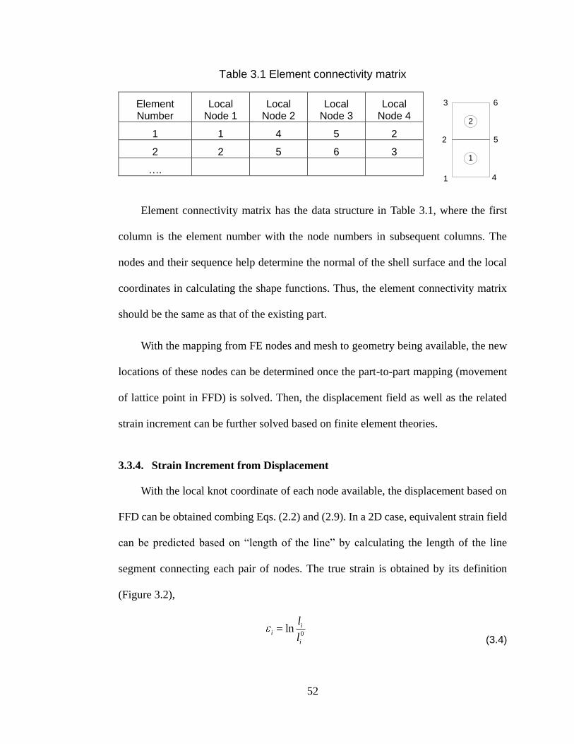
52
Table 3.1 Element connectivity matrix
Element Number
Local Node 1
Local Node 2
Local Node 3
Local Node 4
1 1 4 5 2
2 2 5 6 3
….
1
2
3
4
5
6
1
2
Element connectivity matrix has the data structure in Table 3.1, where the first
column is the element number with the node numbers in subsequent columns. The
nodes and their sequence help determine the normal of the shell surface and the local
coordinates in calculating the shape functions. Thus, the element connectivity matrix
should be the same as that of the existing part.
With the mapping from FE nodes and mesh to geometry being available, the new
locations of these nodes can be determined once the part-to-part mapping (movement
of lattice point in FFD) is solved. Then, the displacement field as well as the related
strain increment can be further solved based on finite element theories.
3.3.4. Strain Increment from Displacement
With the local knot coordinate of each node available, the displacement based on
FFD can be obtained combing Eqs. (2.2) and (2.9). In a 2D case, equivalent strain field
can be predicted based on “length of the line” by calculating the length of the line
segment connecting each pair of nodes. The true strain is obtained by its definition
(Figure 3.2),
0ln i
i
i
l
l
(3.4)
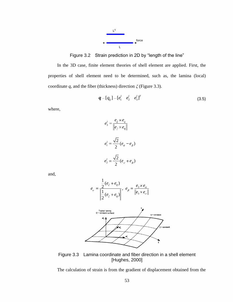
53
L0
L
force
Figure 3.2 Strain prediction in 2D by “length of the line”
In the 3D case, finite element theories of shell element are applied. First, the
properties of shell element need to be determined, such as, the lamina (local)
coordinate q, and the fiber (thickness) direction ξ (Figure 3.3).
1 2 3[ ] [ ]l l l T
ijq e e eq
where,
3
le e
ee e
1
2( )
2
le e e
2
2( )
2
le e e
and,
3
3
1( )
2 , 1
( )2
e ee e
e ee e
e e
(3.5)
Figure 3.3 Lamina coordinate and fiber direction in a shell element [Hughes, 2000]
The calculation of strain is from the gradient of displacement obtained from the
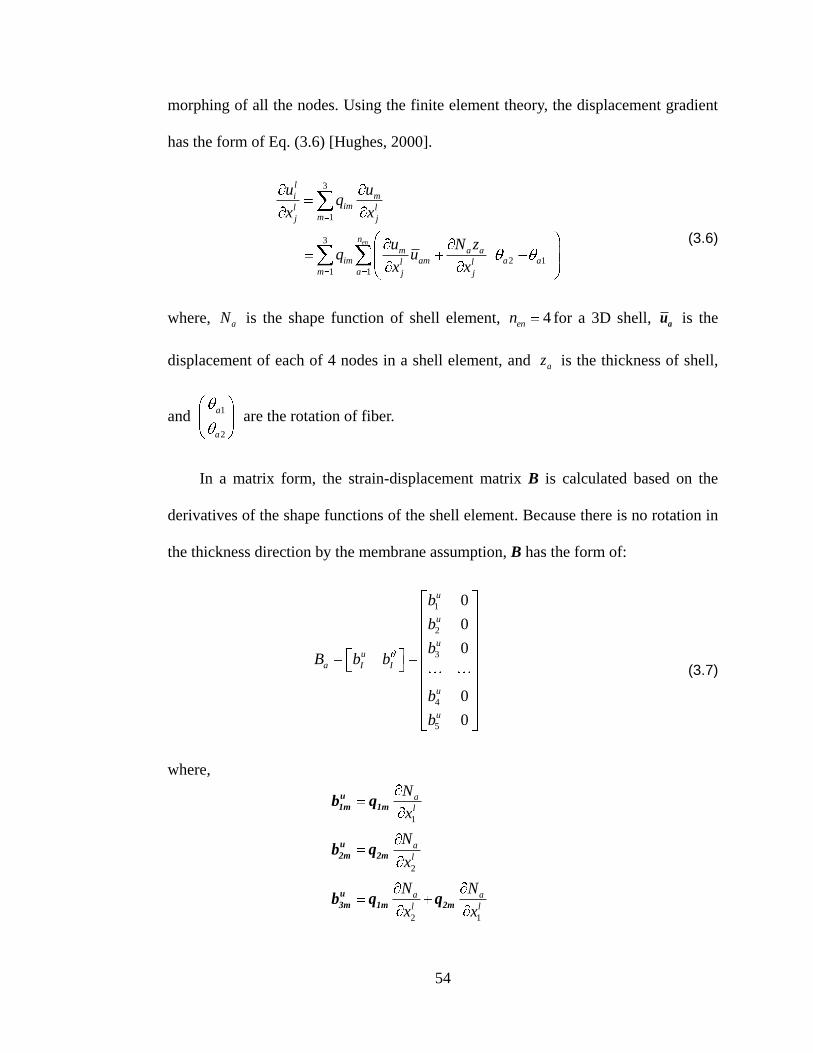
54
morphing of all the nodes. Using the finite element theory, the displacement gradient
has the form of Eq. (3.6) [Hughes, 2000].
3
1
3
2 1
1 1
en
l
i miml l
mj j
n
m a aim am a al l
m a j j
u uq
x x
u N zq u
x x
(3.6)
where, aN is the shape function of shell element, 4enn for a 3D shell, au is the
displacement of each of 4 nodes in a shell element, and az is the thickness of shell,
and 1
2
a
a
are the rotation of fiber.
In a matrix form, the strain-displacement matrix B is calculated based on the
derivatives of the shape functions of the shell element. Because there is no rotation in
the thickness direction by the membrane assumption, B has the form of:
1
2
3
4
5
0
0
0
0
0
u
u
u
u
a I I
u
u
b
b
bB b b
b
b
where,
1
a
l
N
x
u
1m 1mb q
2
a
l
N
x
u
2m 2mb q
2 1
a a
l l
N N
x x
u
3m 1m 2mb q q
(3.7)
55
3 2
a a
l l
N N
x x
u
4m 2m 3mb q q
1 3
a a
l l
N N
x x
u
5m 3m 1mb q q
Finally, strain vectors can be calculated by,
1
1 1
2
0
0
en enn n
a
a a
a
a a
a a
u u
ε B B (3.8)
3.3.5. Bending Energy and Strain Gradient Functions
The strain predicted directly from geometric morphing (3.1) may not have
physical feasibility since there is no material properties related to the geometric
morphing process. And solving the displacement field of the nodes using part-to-part
mapping is different from finite element theory in which the elastic/plastic constitutive
laws are satisfied. Therefore a functional morphing with physical feasibility during
geometric morphing is needed. In order to achieve morphing related physical feasibility,
two conditions are necessary during the geometric morphing: 1) Minimization of
bending energy associated with free-form deformation volume, and 2) Minimization of
the strain gradient on the mapped mesh.
A bending energy function J is introduced to the objective function (3.1) to
minimize the bending energy of the whole FFD volume. This bending energy function
is derived from the strain energy associated with a small deflection of a thin plate
[Ventsel, 2001]. It has been adopted for regularization of problems involving
discontinuities [Terzopoulos, 1986; Sarraga, 2004].
( )J L T dudvdw (3.9)

56
where,
2 2 22 2 2 2 2 2 2 2 2
2 2 2 2 2 2 2 2 2
2 2 22 2 2
( ) 2
2(1 )
T T T T T T T T TL T
u v w u v v w w u
T T T
u v v w w u
3
0
3
0
3
0
,,)()()(),,(
i j k
kjikji wBvBuBzyxT
where ν is the Poisson‟s ratio of the material. In this study, only design surfaces of
products are available and only membrane effect is considered. Therefore ν is chosen to
be 0.5 (incompressible material).
By including the bending energy function (3.9), the optimization problem of (3.1)
is thus equivalent to the Principle of Minimum Potential Energy, where U is the strain
energy stored in an elastic body and the external work W is defined by the loading
condition. Π is the total potential energy in the system. Thus, Eq. (3.10) can be written
as Eq. (3.11) when the total potential energy of a given system has a minimum. The
Principle of Minimum Potential Energy states that considering the small-deflection
theory of an elastic body, the potential energy is a minimum in an equilibrium state.
t b: f f t
T T
V S VU W dV u dV u dV
(3.10)
0 U W (3.11)
where ζ and ε are body stress and strain. u is the vector of displacement. fb and ft are
body force and surface load acting on the volume and boundary St correspondingly.
In this study on sheet metal parts from different generations, since only
geometries are considered and the materials of the parts are assumed to be the same, U
can be regarded as the bending energy function defined in (3.9). W is equivalent to the
57
objective function in (3.1) by satisfying the “pre-scribed boundary” where the general
distance between the parts is minimized. Thus, the solution of optimizing the problem
with including the bending energy function will approximate the equilibrium state.
Minimization of the bending energy related to the whole volume space will lead to
a feasible solution. However, sometimes the solved strain distribution is not uniform
within the part. Therefore, condition 2 focuses locally on the strain distribution of the
part, which is satisfied by introducing a penalty term (3.12) which defines the
summation of strain gradient in all directions:
Let j denote the strain associated with element number j,
ee sd
ii
ee sd n
j
n
i i
jn
j
n
ix
1 1
2
1 1
2j
iiεG (3.12)
where nsd is the dimension and nee is the total number of elements. With such gradient
term, no sharp changes in the strain of adjacent elements are allowed during geometric
morphing but resulting in much smoother increase or decrease.
Integrating (3.1), (3.9) and (3.12), the final optimization problem (3.13) for the
functional morphing between part surfaces is defined by linear combinations of general
distance from registration, bending energy function and strain gradient.
GJPPg TS ),()1( 1Min
s.t.
),(1TSg PP
( )L T dudvdwJ
2
2
1 1 1
ee ee sdn n n
ii
j j i ixiiG ε
(3.13)

58
where,
1 2
, , ,
0 0
3 3 3(0)
, , , ,
0 0 0
3 3 3(0) (0)
, ,
0 0 0
( ) ( ) ( )
( , , ) ( ) ( ) ( )
( , , ) ( ) ( ) ( )
n n
i p j q i j
i j
i j k i j k i j k
i j k
S
i j k i j k
i j k
S N u N v P
T x y z B u B v B w
T x y z B u B v B w
P
P
2 2 2 2 2 22 2 2 2 2 2
2 2 2
2 2 2 2 2 2
2 2 2 2 2 2
( )
+
T T T T T TL T
u v w u v v w w u
T T T T T T
u v v w w u
where α and β are weights valued between 0 and 1, representing trade-offs among the
correspondence, the stored bending energy in FFD volume and strain gradient in the
part surface. Newton-Raphson numerical method is applied to solving the problem.
After solving the mapping functions between existing part and new part, the strain
increment can be obtained from Eqs. (3.4)-(3.8). This strain increment is then
superposed to the strain distribution of the existing part. And the new strain will help
predict the formability using strain-based criteria.
3.4. CASE STUDY
3.4.1. 2D U-shaped Channel Stamping
A 2D U-shaped channel case study similar to Section 2.3.1 has been conducted to
demonstrate the strain increment method. A concave feature (Figure 3.4(C)) is added
into the original part shape (Figure 3.4 (B)). Both ends of the blank are fixed to prevent
material from flowing into the die freely (Figure 3.4 (A)). The purpose of the study is to
generate a new die face to produce the concave feature in the new part and compare the
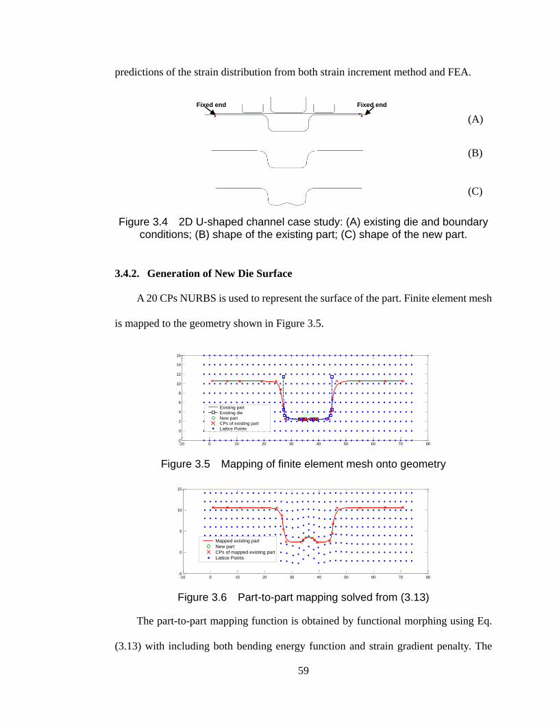
59
predictions of the strain distribution from both strain increment method and FEA.
(A)
(B)
(C)
Figure 3.4 2D U-shaped channel case study: (A) existing die and boundary conditions; (B) shape of the existing part; (C) shape of the new part.
3.4.2. Generation of New Die Surface
A 20 CPs NURBS is used to represent the surface of the part. Finite element mesh
is mapped to the geometry shown in Figure 3.5.
Figure 3.5 Mapping of finite element mesh onto geometry
Figure 3.6 Part-to-part mapping solved from (3.13)
The part-to-part mapping function is obtained by functional morphing using Eq.
(3.13) with including both bending energy function and strain gradient penalty. The
-10 0 10 20 30 40 50 60 70 80-2
0
2
4
6
8
10
12
14
16
-10 0 10 20 30 40 50 60 70 80-5
0
5
10
15
Fixed end Fixed end
Existing part
Existing die
New part
CPs of existing part
Lattice Points
Mapped existing part
New part
CPs of mapped existing part
Lattice Points

60
strain distribution is then calculated and superimposed to the original strain from the
existing part. The linear combination coefficients α and β are chosen to be 0.02 and
0.05 correspondingly. Figure 3.6 shows the mapping between the existing part and the
new part. By close inspection on the movements of all LPs, the whole space is squeezed
upward in the middle to generate the concave shape. Such deformation of the volume
space will result in a small bending energy in order to achieve the concave on the
bottom.
3.4.3. Strain Prediction by Strain Increment Method
Both the strain increment method and finite element analysis are used to calculate
the strain distribution of the new part. Strain distributions of the existing part and the
new part calculated from FEA are shown in Figure 3.7. With the concave feature, there
are two peaks on the walls of the concave because the material on the walls of the
concave is stretched.
Figure 3.7 Strain prediction on the existing and new parts by FEA
0 10 20 30 40 50 60 700
0.05
0.1
0.15
0.2
0.25
Element #
Strai
n
Existing part
New part

61
Figure 3.8 Strain increment
Figure 3.9 Strain prediction by FEA and strain increment method
The strain increment calculated from the strain increment method is shown in
Figure 3.8. Similar peaks are found near the walls. Combining both results, the
comparison of strain increment method and FEA is shown in Figure 3.9. It is seen that,
the strain prediction from the strain increment method without having the new die
shape is well compared with the strain predicted from FEA. This strain distribution can
be further used in formability analysis.
3.4.4. 3D Case Study on Cup Drawing
The same cup drawing case study as in Section 2.3.2 is conducted to demonstrate
the strain increment method in 3D. The new part shape is modified from the original
part shape by adding an increased stamping depth and a concave bottom.
Both the strain increment method and finite element analysis are used to calculate
0 10 20 30 40 50 60 70-0.1
-0.05
0
0.05
0.1
0.15
0.2
0.25
Element #
Strai
n
0 10 20 30 40 50 60 70-0.05
0
0.05
0.1
0.15
0.2
0.25
0.3
Element #
Strai
n
Strain Increment Method
FEA

62
the strain distribution of the new part. Aluminum alloy 6061 has been used for
simulation. The plastic strain distributions (circumferential and radial directions in
cylindrical coordinate, and in-plane maximum principal) of the new part are shown in
Figure 3.10. Both methods are capable to estimate the strain distributions. However,
the strain increment method can be applied without the knowledge of the new die face
and it is more convenient in the product design stage to quickly estimate the formability
a new part design.
(A) Plastic strain in the circumferential
direction from FEA
(B) Plastic strain in the circumferential
direction from strain increment method
(C) Plastic strain in the radial direction
from FEA
(D) Plastic strain in the radial direction
from strain increment method
(E) Plastic strain of maximum in-plane
principal from FEA
(F) Plastic strain of maximum in-plane
principal from strain increment method
Figure 3.10 Strain prediction on the existing and new parts by FEA
0
20
40
60
80
-20
0
20
40
60-10
-5
0
5
10
15
20
XY
-0.0223939
0.00369321
0.0297804
0.0558675
0.0819547
0.108042
0.134129
0
20
40
60
80
-20
0
20
40
60-10
-5
0
5
10
15
20
XY
-0.0352965
-0.00865852
0.0179794
0.0446174
0.0712554
0.0978933
0.124531
010
2030
4050
6070
80
-20
0
20
40
60-10
-5
0
5
10
15
20
XY
0.00653233
0.0280997
0.0496671
0.0712345
0.0928019
0.114369
0.135937
X
Y
Z
rθ
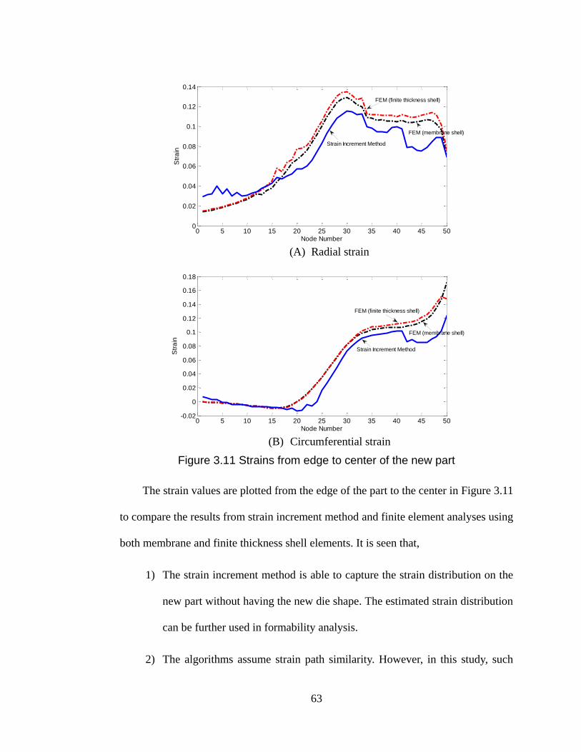
63
(A) Radial strain
(B) Circumferential strain
Figure 3.11 Strains from edge to center of the new part
The strain values are plotted from the edge of the part to the center in Figure 3.11
to compare the results from strain increment method and finite element analyses using
both membrane and finite thickness shell elements. It is seen that,
1) The strain increment method is able to capture the strain distribution on the
new part without having the new die shape. The estimated strain distribution
can be further used in formability analysis.
2) The algorithms assume strain path similarity. However, in this study, such
0 5 10 15 20 25 30 35 40 45 500
0.02
0.04
0.06
0.08
0.1
0.12
0.14
Node Number
Str
ain
Strain Increment Method
FEM (membrane shell)
FEM (finite thickness shell)
0 5 10 15 20 25 30 35 40 45 50-0.02
0
0.02
0.04
0.06
0.08
0.1
0.12
0.14
0.16
0.18
Node Number
Str
ain
Strain Increment Method
FEM (finite thickness shell)
FEM (membrane shell)

64
similarity exists only on the side wall and on the concave bottom of the cup
(except the wall area). Therefore, in regions where there exist strain path
difference, the prediction from the strain increment method has more error
compared with other regions.
3) Discrepancy exists between the predicted strain from strain increment method
and that from FEA. Such discrepancy is mainly from three sources: (i) while
it is the attempt to consider material/process information in functional
morphing, such consideration is still not complete in the functional morphing
algorithms, such as strain path history; (ii) different methodologies are used
to approach equilibrium state. In finite element analysis, the equilibrium is
satisfied during each iteration goverened by constitutive equations, but in the
strain increment method, it is approximated by minimizing the objective
function; (iii) membrane shell ignores the strain distribution in the thickness
direction. The difference in strain distribution using the membrane shell and
the finite thickness shell is shown in Figure 3.11.
3.5. CONCLUSION
Functional morphing enables fast die development through sequential steps of
part-to-part mapping, die-to-die morphing, and finite element verification. Based on
the die face morphing algorithm, a strain increment method has been introduced to
quickly predict the strain and evaluate the formability for a new generation of part. This
method includes mapping of finite element mesh from existing part to the geometry,
calculation of strain using finite element theories, and both bending energy and strain
gradient penalty terms in solving the functional morphing based part-to-part mapping

65
function. By superposition of the strain increment to the original strain distribution
from the existing part, the strain field on the new part can be estimated without the
knowledge of the new die shape. Such strain field can be further used to analyze part
formability. Case studies on a 2D U-shaped channel and a 3D cup drawing demonstrate
the strain increment method and the predicted strain is compared with the FE
simulations in which the new die face is generated by the evolutionary die face
morphing method. Results show that strain increment method is able to capture the
strain distribution on the new part.
Since the strain increment method does not require the knowledge on new die
surface, such formability assessment can be used as an early feasibility assessment of
the new part design. Therefore, it is beneficial to both design and DFE in reducing the
design/manufacturing iterations in stamping development.
REFERENCES
Chen, F. K. and Chiang, B. H., (1998), “Three-Dimensional Finite Element Analysis
for the Stamping of a Motorcycle Oil Tank”, ASME Transactions: Journal of
Manufacturing Science and Engineering, Vol. 120, pp. 770-773.
Chen, L. L., Wang, G. F., Hsiao, K. A. and Liang, J., (2003), “Affective Product Shapes
through Image Morphing”, Proceedings of the International Conference on
Designing Pleasurable Products and Interfaces, pp. 11-16.
Chung, K. and Richmond, O., (1992), “Ideal forming I: Homogeneous deformation
with minimum plastic work”, International Journal of Mechanical Sciences,
Vol. 34, pp. 575-591.
Chung, K. and Richmond, O., (1992), “Ideal forming II: Sheet forming with optimum
deformation”, International Journal of Mechanical Sciences, Vol. 34, pp.
617-633.
Chung, K. and Richmond, O., (1994), “Mechanics of Ideal Forming”, Journal of
Applied Mechanics, Vol. 61, pp. 176-181.

66
Chung, K., Barlat, F., Brem, J. C., Lege, D. J. and Richmond, O., (1997), “Blank Shape
Design for a Planar Anisotropic Sheet Based on Ideal Forming Design Theory
and FEM Analysis”, International Journal of Mechanical Sciences, Vol. 39
(1), pp. 105-120.
Guo, Y. Q., Batoz, J. L., Detraux, J. M. and Duroux, P., (1990), “Finite Element
Procedures for Strain Estimations of Sheet Metal Forming Parts”, International
Journal for Numerical Methods in Engineering, Vol. 30 (8), pp. 1385-1401.
Guo, Y. Q., Batoz, J. L., Naceur, H., Bouabdallah, S., Mercier, F. and Barlet, O., (2000),
“Recent Developments on the Analysis and Optimum Design of Sheet Metal
Forming Parts Using a Simplified Inverse Approach”, Computers and
Structures, Vol. 78 (1), pp. 133-148.
Hong, D., Fadel, G. M. and Blouin, V. Y., (2006), “Vehicle Component Layout with
Shape Morphing - An Initial Study”, Proceedings of 2006 ASME International
Design Engineering Technical Conferences and Computers and Information In
Engineering Conference, DETC 2006.
Hughes, T., (2000), “The Finite Element Method: Linear Static and Dynamic Finite
Element Analysis”, Dover Publications Inc., New York.
Kobayashi, S., Oh, S. and Altan, T., (1989), “Metal Forming and the Finite-Element
Method”, Oxford University Press.
Lan, J., Dong, X. and Li, Z., (2005), “Inverse Finite Element Approach and Its
Application in Sheet Metal Forming”, Journal of Materials Processing
Technology, Vol. 170 (3), pp. 624-631.
Lin, G., Li, J., Hu, S. J. and Cai, W., (2007), “A Computational Response Surface Study
of Three-Dimensional Aluminum Hemming Using Solid-to-Shell Mapping”,
Transactions of the ASME: Journal of Manufacturing Science and Engineering,
Vol. 129, pp. 360-368.
Naceur, H., Guo, Y. Q. and Batoz, J. L., (2004), “Blank Optimization in Sheet Metal
Forming Using an Evolutionary Algorithm”, Journal of Materials Processing
Technology, Vol. 151 (1-3), pp. 183-191.
Ryou, H., Chung, K., Yoon, J. W., Han, C. K., Youn, J. R. and Kang, T. J., (2005),
“Incorporation of Sheet-Forming Effects in Crash Simulations Using Ideal
Forming Theory and Hybrid Membrane and Shell Method”, ASME
Transactions: Journal of Manufacturing Science and Engineering, Vol. 127 (1),
pp. 182-192.
Sabourin, F., Morestin, F. and Brunet, M., (2004), “Sheet Forming with a Specific
Inverse Approach for a Further Springback Analysis”, AIP Conference
Proceedings, Vol. 712, pp. 832-837.

67
Saran, M. J., Schedin, E., Samuelsson, A., Melander, A. and Gustafsson, C., (1990),
“Numerical and Experimental Investigations of Deep Drawing of Metal
Sheets”, Journal of Engineering for Industry, Vol. 112, pp. 272-277.
Sarraga, R., (2004), “Modifying CAD/CAM Surfaces According to Displacements
Prescribed at a Finite Set of Points”, Computer Aided Design, Vol. 36, pp.
343-349.
Sederberg, T. and Parry, S., (1986), “Free-Form Deformation of Solid Geometric
Models”, Computer Graphics, Vol. 20, pp. 151-160.
Terzopoulos, D., (1986), “Regularization of Inverse Visual Problems Involving
Discontinuities”, IEEE Transactions on Pattern Analysis and Machine
Intelligence, Vol. 8 (4), pp. 413-424.
Ventsel, E. and Krauthammer, T., (2001), “Thin Plates and Shells: Theory, Analysis,
and Applications”, Marcel Dekker, New York.
Zhou, L., Hu, S. J., Lin, G. and Stoughton, T.B., (2009), “Evolutionary Stamping Die
Development Using Morphing Technology”, Transactions of the NAMRI/SME,
Vol. 37.
68
CHAPTER 4 3
FUNCTIONAL MORPHING IN MULTI-STAGE
MANUFACTURING AND ITS APPLICATIONS IN
HIGH-DEFINITION METROLOGY BASED PROCESS
CONTROL
ABSTRACT
In multi-stage manufacturing processes equipped with high-definition metrology
(HDM), part shapes can be observed to morph throughout the machining stages in
multiple deformation scales, which is caused by the interaction between machining
stages and physical attributes of the parts, as defined by functional morphing.
Functional morphing characterizes the dependence of surface characteristics at
downstream stages on surface characteristics from upstream stages. Conventional
methodology to study the inter-stage relationship focuses on variation propagation of
discrete key product characteristics or surface vectors and has limitations in analyzing
HDM data for complex shape changes. This chapter investigates the functional
morphing and explores its applications in improving variation reduction strategy. A
functional free form deformation approach is developed to extract mapping functions
between manufacturing stages. The obtained mapping functions enable multi-scale
Contents of this chapter are to be submitted to IEEE Transactions: Automation Science and
Engineering.

69
variation propagation analysis and intermediate stage process monitoring. It also
allows for accurate inter-stage adjustment that introduces shape deformation upstream
to compensate for the end-of-line errors. The developed monitoring and adjustment
algorithms are demonstrated via a case study of a two-stage machining process. Other
application such as process tolerance design is also discussed.
4.1. INTRODUCTION
High-definition metrology (HDM), a new surface inspection technology with high
resolution, has become a key enabler of high-precision manufacturing. Figure 4.1
shows a scanned surface on a V-8 engine head, where the color indicates the height
measurement (μm). It can be seen that the surface is of a “bowl” shape form.
Meanwhile, features in small scale related to tooling conditions (e.g., tool mark) are
also observed. When HDM is applied to a multistage manufacturing process, the
changes of part surfaces from stage to stage in a complex manner can be analyzed as
morphing. The inter-stage changes may occur at multiple scales: global shape, local
defects with different sizes, and waviness. Figure 1.3 shows a two-stage machining
process that mills the part top surface (Op1) followed by a drilling operation on its side
(Op2). It can be seen from Figure 1.3(C, D) that surface exiting Op2 differs from Op1
in both global shape and local defect (a small bump in the middle).
Figure 4.1 V-8 engine head measured by HDM device
70
In a multistage machining process, the part surface change includes shape,
waviness, and key product characteristics that reflect the inter-stage interaction of
given process settings and part physical properties such as mass density, casting pore
distribution, and mechanical properties. For instance, Figure 1.3 describes the change
from 2 operations: milling and drilling. Such change is the result of the joint effect of
the geometrical shape due to the cutter path and the mechanical/materials interactions
of cutting force, deformation and springback. Therefore, functional morphing is
needed to describe the part feature change between stages caused by the process
conditions and part physical properties, instead of using pure geometric morphing.
In computer graphics, morphing patterns are captured by mathematical
transformation which maps any point on the source object to the corresponding point
on the target object. The most commonly used transformation techniques include affine
transformation and quadratic transformation [Hearn and Baker, 1994], Thin Plate
Spline (TPS) [Bookstein, 1989], and Free-Form Deformation (FFD) [Sederberg, 1986;
Coquillart, 1990]. The affine transformation is usually utilized for rigid body but lacks
the degrees of freedom to describe the complex shape changes. Quadratic
transformation offers more but still limited degrees of freedom. TPS and FFD are
commonly adopted approaches for an accurate characterization of surfaces with
global-local feature changes. However, these methods are data-oriented and may yield
transformations that are difficult to interpret since no physical insights are provided.
For the control of a multistage manufacturing process, it is necessary to extend from the
geometry morphing to the functional morphing.
Existing research on manufacturing process control focuses on the variation
71
propagation that investigates the variations accumulated through upstream stages and
their impact on current and downstream stages, as reviewed by [Shi, 2006]. This line of
research includes multistage variation propagation modeling [Mantripragada and
Whitney, 1999; Jin and Shi, 1999; Djurdjanovic and Ni, 2001; Zhou, et al. 2003;
Camelio, et al. 2003], model based process fault diagnosis [Ding, et al. 2002; Zhou, et
al. 2004], multistage process tolerance design [Huang and Shi, 2003; Ding, et al. 2005],
as well as process adjustment with programmable toolings [Wang and Huang, 2007;
Zhong, et al. 2009]. Utilizing vectorial surface model [Huang, et al. 2003] or discrete
nodes (obtained from CMM scanning or finite element analysis) to represent the
surface shape [Camelio, et al. 2003], these methods modeled functional morphing
either by engineering knowledge such as rigid body kinematics for rigid parts [Cai, et al.
1996] and finite element analysis for compliant parts [Camelio, et al. 2003], or by data
driven approach [Apley and Shi, 2001; Liu, et al. 2008].
The aforementioned approaches used vectorial surface model and vector of
low-dimensional scanned data or FEM nodes to represent part surfaces. However, they
are not appropriate for HDM data analysis. The vectorial surface model presents
limited surface information in that it mainly captures the features with regular shape
such as planar or cylindrical. And using FEM nodes could increase the computational
load exponentially due to fine meshing. Furthermore, these approaches did not
distinguish feature changes in different scales such as global shape, local deformation,
or surface waviness and therefore the number of variation sources considered in
variation propagation modeling is limited (e.g., cutter‟s condition and cutting force,
variation of material properties). Engineering process models should be used in
72
conjunction with morphing technology in computer graphics to derive the functional
morphing.
This chapter develops functional morphing modeling for process variation
propagation analysis in a multistage machining process. Functional morphing models
are established based on the morphing technology in computer graphics among part
features. The extracted morphing patterns are applied in process control including
inter-stage process monitoring and adjustment and process design.
This chapter is organized as follows: Section 4.2 develops functional morphing
modeling and extracts morphing pattern based on free-form deformation (FFD), by
which the surface variation propagation is derived from HDM data. Section 4.3
presents the detailed algorithms in morphing based process monitoring and control.
The proposed algorithms are then demonstrated by a case study in Section 4.4.
Conclusions are drawn in Section 4.5.
4.2. MODELING OF SURFACE CHANGES USING FUNCTIONAL
MORPHING
Conventional morphing is a mapping between geometries where only pure
geometric relationship is considered. Functional morphing incorporates mechanical
properties in addition to geometric relationship, so that physical feasibility is satisfied
in a geometric mapping process. This section develops functional morphing to model
surface changes between stages using feature extraction of HDM data, forward and
backward mapping functions, and variation propagation through morphing.

73
4.2.1. Feature Extraction
Although HDM measurements can provide rich information on different scales
of features and the associated process conditions, HDM data may have redundancy
and cause unnecessary computational load. Thus, HDM data should be preprocessed
to the scale of interest. For example, global flatness is evaluated at a large scale, while
waviness or tool mark may require a much smaller scale.
The metrology using laser holographic interferometry produces scattered data for
x, y, and z coordinates on a machined surface. For variation control, the primary
concern is to analyze height (z) values that are spatially distributed along the x and y
directions. One way to extract such feature is to project the scattered HDM data onto
rectangular grids through interpolation and extrapolation methods, where the size of
the grids determines the scale of study, i.e., coarse grid extracts global scale features
(e.g., global flatness), while dense grid extracts small scale features (e.g., tool mark).
Figure 4.2 shows an example of using triangle interpolation to obtain surface grids,
where zi‟s are scattered data from measurements and 'iz ‟s are the projected data on
grids. The objective is to find an interpolation method A and 'z such that,
2
, 'min 'A Az z z (4.1)
where 1 2[ ...]Tz zz = and ' '
1 2[ ...]Tz zz = . For detailed procedures, refer to [Keim and
Herrmann, 1998].
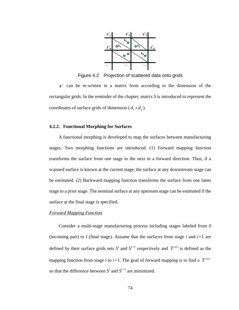
74
Figure 4.2 Projection of scattered data onto grids
'z can be re-written in a matrix form according to the dimension of the
rectangular grids. In the reminder of the chapter, matrix S is introduced to represent the
coordinates of surface grids of dimension ( 1 2d d ).
4.2.2. Functional Morphing for Surfaces
A functional morphing is developed to map the surfaces between manufacturing
stages. Two morphing functions are introduced: (1) Forward mapping function
transforms the surface from one stage to the next in a forward direction. Thus, if a
scanned surface is known at the current stage, the surface at any downstream stage can
be estimated. (2) Backward mapping function transforms the surface from one latter
stage to a prior stage. The nominal surface at any upstream stage can be estimated if the
surface at the final stage is specified.
Forward Mapping Function
Consider a multi-stage manufacturing process including stages labeled from 0
(incoming part) to I (final stage). Assume that the surfaces from stage i and i+1 are
defined by their surface grids sets Si and S
i+1 respectively and
1,i iT is defined as the
mapping function from stage i to i+1. The goal of forward mapping is to find a 1,i iT
so that the difference between Si and S
i+1 are minimized.
z‟1 z‟2 z‟3
z‟4 z‟6
… … …
z1
z2
z3
z4
z‟1 z‟2 z‟3
z‟4 z‟6
… … …
z1
z2
z3
z4
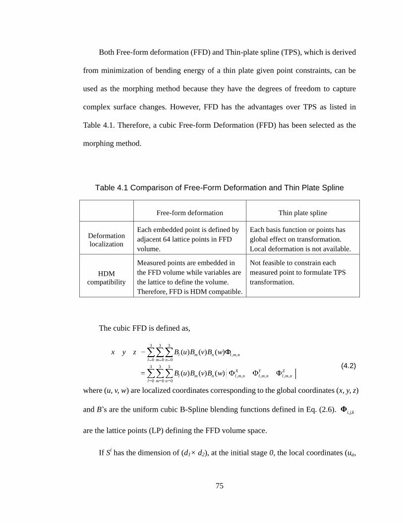
75
Both Free-form deformation (FFD) and Thin-plate spline (TPS), which is derived
from minimization of bending energy of a thin plate given point constraints, can be
used as the morphing method because they have the degrees of freedom to capture
complex surface changes. However, FFD has the advantages over TPS as listed in
Table 4.1. Therefore, a cubic Free-form Deformation (FFD) has been selected as the
morphing method.
Table 4.1 Comparison of Free-Form Deformation and Thin Plate Spline
Free-form deformation Thin plate spline
Deformation
localization
Each embedded point is defined by
adjacent 64 lattice points in FFD
volume.
Each basis function or points has
global effect on transformation.
Local deformation is not available.
HDM
compatibility
Measured points are embedded in
the FFD volume while variables are
the lattice to define the volume.
Therefore, FFD is HDM compatible.
Not feasible to constrain each
measured point to formulate TPS
transformation.
The cubic FFD is defined as,
3 3 3
, ,
0 0 0
3 3 3
, , , , , ,
0 0 0
( ) ( ) ( )
( ) ( ) ( )
l m n l m n
l m n
X Y Z
l m n l m n l m n l m n
l m n
x y z B u B v B w
B u B v B w (4.2)
where (u, v, w) are localized coordinates corresponding to the global coordinates (x, y, z)
and B‟s are the uniform cubic B-Spline blending functions defined in Eq. (2.6). i, j,kΦ
are the lattice points (LP) defining the FFD volume space.
If Si has the dimension of (d1× d2), at the initial stage 0, the local coordinates (ua,
76
va, wa) of point 0
aS in 0S , 21 ... 1 dda , are determined by (4.3),
3 3 30 0
0 0 0 0 , ,
0 0 0
| ( | ) ( | ) ( | )a l a m a n a l m n
l m n
S B u B v B w Φ (4.3)
where 0Φ is the initial FFD volume space. The notation 0| denotes that is
measured at stage 0. The local coordinates determined at stage 0 are invariant for the
morphing over the subsequent stages.
In FFD, new surface is generated by deforming the volume space Φ . Thus, at any
stage i, the surface grids Si can be written as,
3 3 3
0 0 0 0 , ,
0 0 0
| ( | ) ( | ) ( | )i i
a l a m a n a l m n
l m n
S B u B v B w Φ (4.4)
where iΦ is the FFD volume space at stage i.
Definition 1: Continuous Forward Mapping
Define ,j i
Φ be the deformation of FFD volume space from stage i to j.
Continuous forward mapping states that the volume space at any stage after
measurement at stage (i) is determined by the summation of all mapping functions from
stage j to i.
, 1, , 1 ( )j i j i i i i j j i jΦ Φ Φ Φ Φ Φ
Then,
3 3 3
0 0 0
1, , 1
, , , , , ,
ˆ | ( | ) ( | ) ( | )
j
a i l a i m a i n a i
l m n
i i i j j
l m n l m n l m n
S B u B v B w
Φ Φ Φ
where ˆ |j
a iS is the estimated surface grid matrix at stage i.
(4.5)
An optimization problem (4.6) considering only geometric relationship is

77
formulated to solve the mapping function 1,i iΦ for 2 consecutive stages.
1,
1
1 ( | , | )i i
i i
i ig S SΦ
Min
s.t. 1
1( | , | )i i
i ig S S (4.6)
where 1g is a mutual distance function measuring the distance between two surfaces
defined by surface grids, and is the maximum registration error between the surface
grids at stage i and i+1.
The solution to (4.6) is not unique, and constraints and penalty functions governed
by physical laws are needed to ensure the feasible solution region. In this study, the
penalty function is chosen to be bending energy J defined in Eq. (4.7), which is derived
from the strain energy associated with a small deflection of a plate [Ventsel and
Krauthammer, 2001].
( )J L dudvdwT
where,
2 2 22 2 2 2 2 2 2 2 2
2 2 2 2 2 2 2 2 2
2 2 22 2 2
( ) 2
2(1 )
L Du v w u v v w w u
u v v w w u
T T T T T T T T TT
T T T
and,
3
2
3 3 3
, ,
0 0 0
( , , ) ( , , )( , , )
12(1 )
( ) ( ) ( )l m n l m n
l m n
E u v w h u v wD u v w
B u B v B wT Φ
(4.7)
where E is the Young‟s modulus, h is an equivalent thickness function derived from the
real part and ν is the Poisson‟s ratio. Space-varying variable D can characterize
heterogeneous properties of parts.

78
Similar to the bending energy of FFD volume defined in Chapter 3 for strain
increment method, the optimization problem (4.6) is also equivalent to the Principle of
Minimum Potential Energy in Eq. (4.8) by including the energy term in Eq. (4.7) with
extended physical properties. In Eq. (4.8), δU is the change of strain energy stored in an
elastic body and the change of external work δW is defined by the loading condition. Π
is the total potential energy. The solution to Eq. (4.8) results in an equilibrium state.
0 U W
(4.8)
In our study where the material remains the same throughout the manufacturing
process, U can be regarded as the bending energy defined in (4.7). W is equivalent to
the objective function in (4.6) by satisfying the “pre-scribed boundary” where the
mutual distance between the part surfaces is minimized. Thus, the solution to the
optimization problem (4.6) combined with (4.7) will approximate the equilibrium state.
Finally, a new optimization problem is formulated in (4.9).
1,
1
1(1 ) ( | , | )+i i
i i
i ig S S JΦ
Min (4.9)
where is the optimization parameter between 0 and 1, which indicates the trade-off
between registration error and stored bending energy inside FFD volume.
Backward mapping function
Similar to the forward mapping which considers the mapping from a previous
stage to a latter one, when the desired final surface at stage (I) IIS | is specified, the
nominal surface shape (or desired surface shape) at any previous stage i can be
estimated by using backward mapping.
The backward mapping function can be derived based on the forward mapping
function by sharing the same FFD volume space iΦ ( 1...i I ) at each stage. Given the
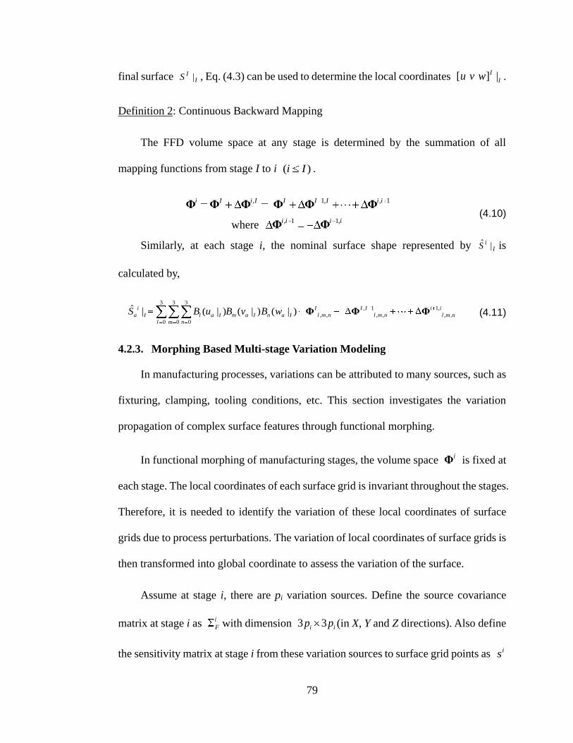
79
final surface IIS | , Eq. (4.3) can be used to determine the local coordinates [ ] |I
Iu v w .
Definition 2: Continuous Backward Mapping
The FFD volume space at any stage is determined by the summation of all
mapping functions from stage I to i ( )i I .
, 1, , 1 i I i I I I I i iΦ Φ Φ Φ Φ Φ
where , 1 1,i i i i
Φ Φ (4.10)
Similarly, at each stage i, the nominal surface shape represented by IiS |ˆ is
calculated by,
3 3 3, 1 1,
, , , , , ,
0 0 0
ˆ | ( | ) ( | ) ( | )i I I I i i
a I l a I m a I n a I l m n l m n l m n
l m n
S B u B v B w Φ Φ Φ (4.11)
4.2.3. Morphing Based Multi-stage Variation Modeling
In manufacturing processes, variations can be attributed to many sources, such as
fixturing, clamping, tooling conditions, etc. This section investigates the variation
propagation of complex surface features through functional morphing.
In functional morphing of manufacturing stages, the volume space i
Φ is fixed at
each stage. The local coordinates of each surface grid is invariant throughout the stages.
Therefore, it is needed to identify the variation of these local coordinates of surface
grids due to process perturbations. The variation of local coordinates of surface grids is
then transformed into global coordinate to assess the variation of the surface.
Assume at stage i, there are pi variation sources. Define the source covariance
matrix at stage i as i
F with dimension 3 3i ip p (in X, Y and Z directions). Also define
the sensitivity matrix at stage i from these variation sources to surface grid points as is

80
with the dimension of 1 23( ) 3 id d p , which measures how a unit change in variation
sources impacts the change of surface grids. In the global Cartesian coordinate, the
variation of the surface grids i
SF can be calculated by,
( )i i i i T
SF Fs s (4.12)
The surface grid variation iSF in the local coordinate can be calculated as,
1
1
1 1
( ) ( )
( ) ( ) ( )
( ) ( )
i i i i T
SF SF
i i i i T i T
F
Ti i i i i
F
J J
J s s J
J s J s
(4.13)
where iJ is the Jacobian matrix at stage i expressed as,
1,1 1,1 1,1
1,1 1,1 1,1
1,1 1,1 1,1
, , ,
, , ,
,
1,1 1,1 1,1
1,1 1,1 1,1
1,1 1,1 1,1
, , ,
, , ,
0 0
0 0
[ ]
a b a b a b
a b a b a b
a b
i i i
X X X
i i i
Y Y Y
ii iZZ Z
i i i
X X X
a b a b a b
i i iiY Y Y
a b a b a b
i
Z
S S S
u v w
S S S
u v w
SS S
u v w
S S S
u v w
S S SJ
u v w
S, ,
( ),( ) ( ),( ) ( ),( )1 2 1 2 1 2 1 2 1 2 1 2
1 2 1 2 1 2
( ),( ) ( ),( ) ( ),( )1 2 1 2 1 2 1 2 1 2 1 2
1 2 1 2 1 2
( ),(1 2
, , ,
0 0
a b a b
d d d d d d d d d d d d
d d d d d d d d d d d d
d d
i i
Z Z
a b a b a b
i i i
X X X
d d d d d d
i i i
Y Y Y
d d d d d d
Z
S S
u v w
S S S
u v w
S S S
u v w
S) ( ),( ) ( ),( )1 2 1 2 1 2 1 2 1 2
1 2 1 2 1 2
,
,
d d d d d d d d d d
i i i
Z Z
d d d d d d
i
a b
a b
S S
u v w
Sdiag
U
(4.14)
where 10 da and 20 db . The partial derivatives in Eq. (4.14) can be evaluated
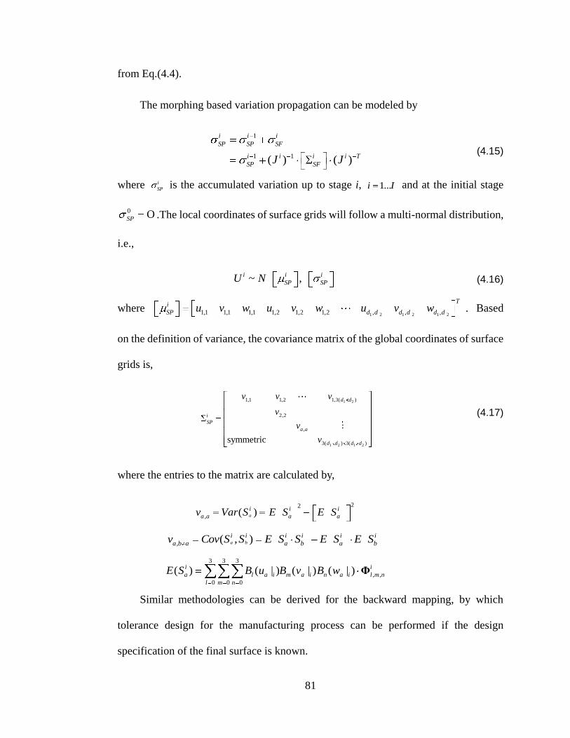
81
from Eq.(4.4).
The morphing based variation propagation can be modeled by
1
1 1( ) ( )
i i i
SP SP SF
i i i i T
SP SFJ J (4.15)
where i
SP is the accumulated variation up to stage i, Ii ...1 and at the initial stage
0 OSP .The local coordinates of surface grids will follow a multi-normal distribution,
i.e.,
~ , i i i
SP SPU N (4.16)
where 1 2 1 2 1 21,1 1,1 1,1 1,2 1,2 1,2 , , ,
Ti
SP d d d d d du v w u v w u v w . Based
on the definition of variance, the covariance matrix of the global coordinates of surface
grids is,
1 2
1 2 1 2
1,1 1,2 1,3( )
2,2
,
3( ) 3( )symmetric
d d
i
SP
a a
d d d d
v v v
v
v
v
where the entries to the matrix are calculated by,
22
, ( )a
i i i
a a a av Var S E S E S
, ( , )a b
i i i i i i
a b a a b a bv Cov S S E S S E S E S
3 3 3
, ,
0 0 0
( ) ( | ) ( | ) ( | )i i
a l a i m a i n a i l m n
l m n
E S B u B v B w Φ
(4.17)
Similar methodologies can be derived for the backward mapping, by which
tolerance design for the manufacturing process can be performed if the design
specification of the final surface is known.

82
4.3. APPLICATIONS OF FUNCTIONAL MORPHING IN MACHINING
PROCESS CONTROL
Using the morphing based variation propagation model, this section discusses
three potential applications for machining process control including inter-stage process
adjustment, process monitoring and tolerance design.
4.3.1. Inter-stage Process Adjustment
Functional morphing can be utilized to conduct an inter-stage process adjustment
by introducing deformation upstream to compensate for the end-of-line errors. The
artificially introduced deformation can be generated by adjusting process variables
such as fixturing, clamping, and machining parameters. The advantage of the
inter-stage process adjustment is that the compensation of complex form errors can be
allocated onto multiple stages, thus reducing adjustment cost for each stage.
Consider a multi-stage manufacturing system as shown in Table 4.2. Assume that
the measurement is conducted at stage i. The optimal strategy should apply adjustments
from stage i to I so that the surface at the end stage is as close as to the desired shape
IIS | with a minimum variance. The formulation is given in Eq. (4.18), where the
continuous forward mapping is used to estimate the surface at the final stage.
Meanwhile, the objective is obtained similar to the signal-to-noise ratio (SNR)
[Taguchi, 1986; Wu and Hamada, 2000] by calculating the inverse of sum square error
of surface grids over the sum of their variances.

83
Table 4.2 Manufacturing system for inter-stage error compensation
Stage 0 … Stage i Stage i+1 … Stage I
Shape
Surface Grids S0 Si Si+1 SI
FFD lattice Φ0 Φi Φi+1 ΦI
Covariance matrix 0F i
F 1iF I
F
( ) 10 2
10 10
1 110 log
ˆˆ || |
ˆ ˆ 10 2 log | | log |
j i j I II ISP ii I
I I I
i I SP i
traceS S
S S trace
Max
s.t.
jjjUL for all )( Iji
where,
3 3 3
, ,
0 0 0
ˆ | ( | | ) ( | | ) ( | | )I I II I
a i l a i a j m a i a j n a i a j l m nj i j i j il m n
S B u u B v v B w w Φ
( 1 21...a d d , | , | , |a j a j a ju v w is change of local coordinates of
surface grids due to the adjustments j with upper and lower limits being
jU and
jL , respectively.)
1 1 1( ) ( )i i i i i i i T
SP SP SF SP SFJ J
i
SP is derived based on i
SP using Eq. (4.17).
(4.18)
The solution to (4.18) gives the optimal adjustment strategy from the
measurement stage i to the end of the manufacturing process.
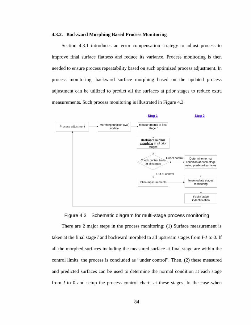
84
4.3.2. Backward Morphing Based Process Monitoring
Section 4.3.1 introduces an error compensation strategy to adjust process to
improve final surface flatness and reduce its variance. Process monitoring is then
needed to ensure process repeatability based on such optimized process adjustment. In
process monitoring, backward surface morphing based on the updated process
adjustment can be utilized to predict all the surfaces at prior stages to reduce extra
measurements. Such process monitoring is illustrated in Figure 4.3.
Check control limits
at all stages
Measurements at final
stage I
Backward surface
morphing at all prior
stages
Determine normal
condition at each stage
using predicted surfaces
Intermediate stages
monitoringInline measurements
Faulty stage
indentification
Under control
Out-of-control
Step 1 Step 2
Process adjustmentMorphing function (ΔΦi
)
update
Figure 4.3 Schematic diagram for multi-stage process monitoring
There are 2 major steps in the process monitoring: (1) Surface measurement is
taken at the final stage I and backward morphed to all upstream stages from I-1 to 0. If
all the morphed surfaces including the measured surface at final stage are within the
control limits, the process is concluded as “under control”. Then, (2) these measured
and predicted surfaces can be used to determine the normal condition at each stage
from I to 0 and setup the process control charts at these stages. In the case when
85
measured surface at final stage and/or some morphed surfaces at prior stages are
out-of-control, then inline measurements are taken at these stages and fed into control
charts to localize faulty stages. Compared with 100% inspection at all stages, the
proposed monitoring strategy requires fewer measurements.
The covariance matrix for the surface grids IISF | is first determined by a number
of measured parts to setup the control limits at the final stage. These surface grids
follow a multi-normal distribution ,I I
SFN S , where averaged surface IS estimates
the mean and multivariate monitoring methods can be applied for statistical process
control. Since the monitored surface grids, IS ‟s, can be highly spatial correlated,
dimension reduction techniques, such as Principal Component Analysis (PCA), can be
applied to filter out redundant information and reduce the misdetection rate. Process
control charts for intermediate stages can be constructed similarly by estimating the
surface grids using backward mapping functions (4.10)-(4.11) if the measured surfaces
from final stage I are all under control.
Once an out-of-control is detected at some stage, backward mapping will no long
work since it was established based on normal conditions. Further measurements are
needed at prior stages to identify the faulty stage as well as root causes.
4.3.3. Process Tolerance Design
Variation propagation modeling derived using forward morphing (Eq. (4.5)) could
improve the tolerance stackup prediction and tolerance allocation that minimizes the
tooling cost while ensures the final product dimensional tolerance. Typically,
minimizing tooling cost is equivalent to maximizing the sum of process tolerances. Let
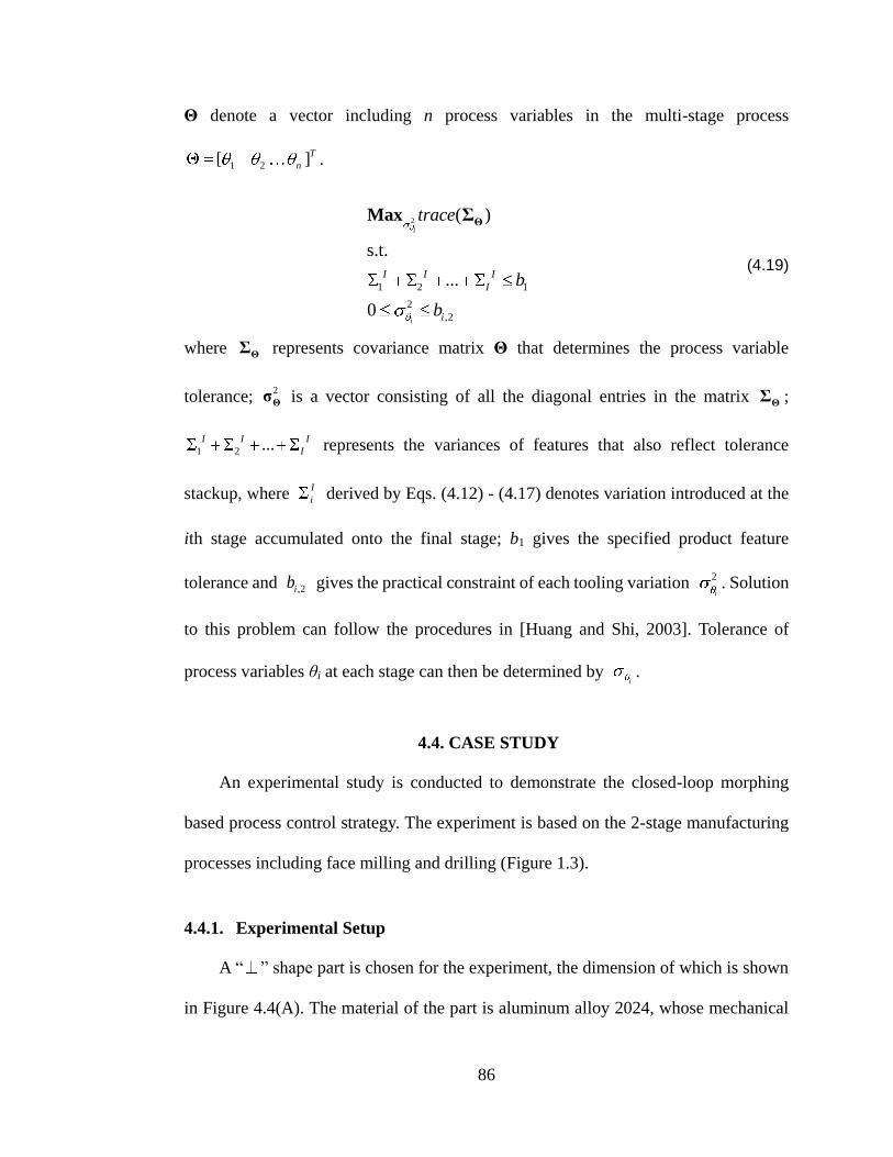
86
Θ denote a vector including n process variables in the multi-stage process
1 2[ ]T
n .
2
1 2 1
2
,2
( )
s.t.
...
0
i
i
I I I
I
i
trace
b
b
ΘMax Σ
(4.19)
where ΘΣ represents covariance matrix Θ that determines the process variable
tolerance; 2
Θσ is a vector consisting of all the diagonal entries in the matrix ΘΣ ;
1 2 ...I I I
I represents the variances of features that also reflect tolerance
stackup, where I
i derived by Eqs. (4.12) - (4.17) denotes variation introduced at the
ith stage accumulated onto the final stage; b1 gives the specified product feature
tolerance and ,2ib gives the practical constraint of each tooling variation 2
i. Solution
to this problem can follow the procedures in [Huang and Shi, 2003]. Tolerance of
process variables θi at each stage can then be determined by i.
4.4. CASE STUDY
An experimental study is conducted to demonstrate the closed-loop morphing
based process control strategy. The experiment is based on the 2-stage manufacturing
processes including face milling and drilling (Figure 1.3).
4.4.1. Experimental Setup
A “ ” shape part is chosen for the experiment, the dimension of which is shown
in Figure 4.4(A). The material of the part is aluminum alloy 2024, whose mechanical
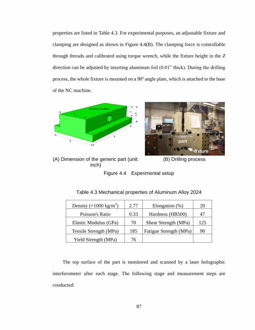
87
properties are listed in Table 4.3. For experimental purposes, an adjustable fixture and
clamping are designed as shown in Figure 4.4(B). The clamping force is controllable
through threads and calibrated using torque wrench, while the fixture height in the Z
direction can be adjusted by inserting aluminum foil (0.01” thick). During the drilling
process, the whole fixture is mounted on a 90º angle plate, which is attached to the base
of the NC machine.
5
3
1.5
1
2
0.7
5monitored surface
(A) Dimension of the generic part (unit:
inch) (B) Drilling process
Figure 4.4 Experimental setup
Table 4.3 Mechanical properties of Aluminum Alloy 2024
Density (×1000 kg/m3) 2.77 Elongation (%) 20
Poisson's Ratio 0.33 Hardness (HB500) 47
Elastic Modulus (GPa) 70 Shear Strength (MPa) 125
Tensile Strength (MPa) 185 Fatigue Strength (MPa) 90
Yield Strength (MPa) 76
The top surface of the part is monitored and scanned by a laser holographic
interferometer after each stage. The following stage and measurement steps are
conducted:

88
1) Face mill the top surface and take the initial measurement before releasing the
clamping. The measured surface profile is regarded as incoming surface.
2) Take the second measurement after releasing the clamping. By releasing the
clamping forces, some deformation on the top surface will be recovered
depending on the magnitude of the clamping forces.
3) Mount the part back to the fixture, drill the side hole (Figure 4.4(B)) and then
take the third measurement on the top surface after releasing from fixture. It is
expected that localized defect on the top surface will be generated due to
drilling.
4.4.2. Functional Morphing Between Stages
The forward mapping method in Section 4.2.2 is utilized to establish the
functional morphing between stages. Before mapping, the global feature is extracted
through triangular interpolation as shown in Figure 4.5. The data dimension is reduced
from 150k to 800 points on regularized grids.
Results of the functional morphing are shown in Figure 4.6 for both stages. The
coefficient α in the optimization is chosen to be 0.01 which is believed to well
incorporate the physical feasibility of each stage. It is seen that, after releasing the
clamping forces in the face milling stage, the surface tends to bend downward (Figure
4.6(B, D)). After the drilling stage, a local defect (bump) is created in the middle of the
top surface due to drill torque (Figure 4.6(C, E)).
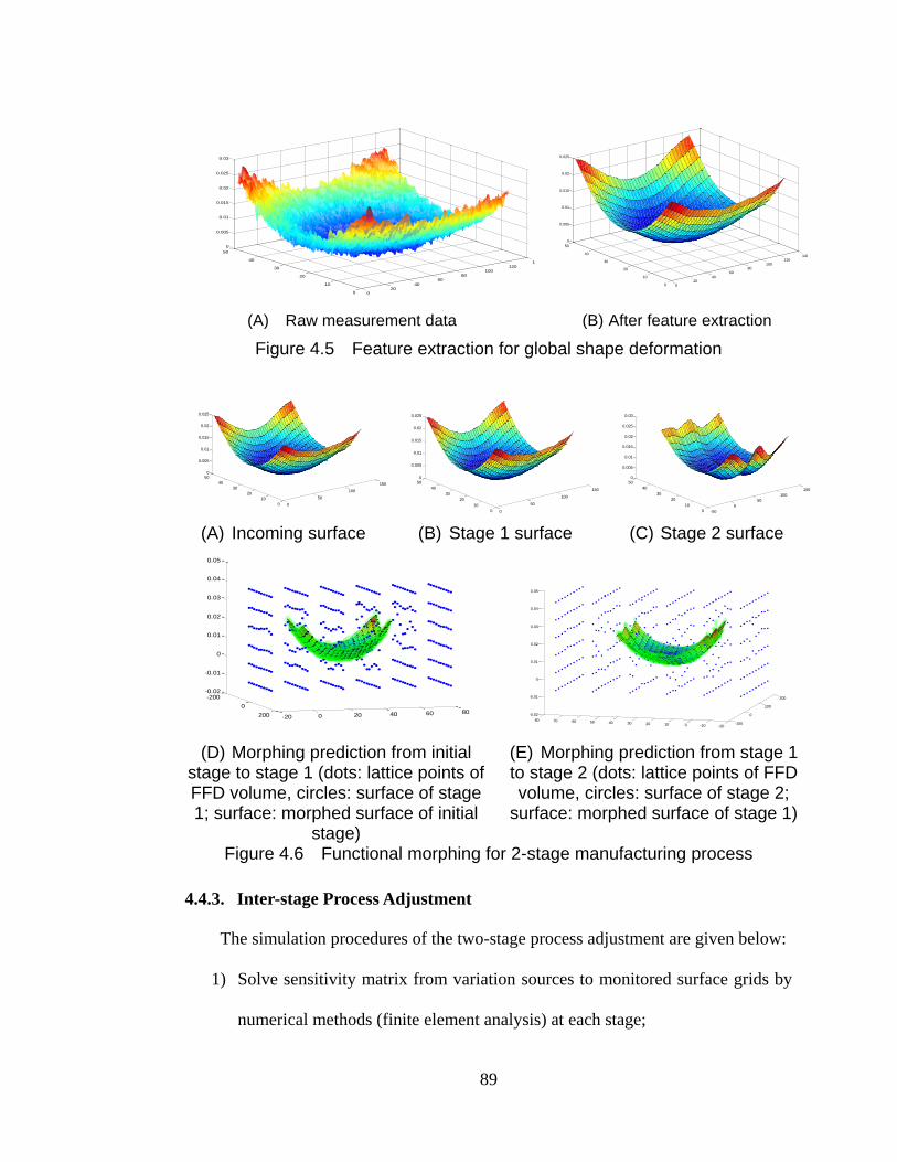
89
(A) Raw measurement data (B) After feature extraction
Figure 4.5 Feature extraction for global shape deformation
(A) Incoming surface (B) Stage 1 surface (C) Stage 2 surface
(D) Morphing prediction from initial stage to stage 1 (dots: lattice points of FFD volume, circles: surface of stage 1; surface: morphed surface of initial
stage)
(E) Morphing prediction from stage 1 to stage 2 (dots: lattice points of FFD volume, circles: surface of stage 2;
surface: morphed surface of stage 1)
Figure 4.6 Functional morphing for 2-stage manufacturing process
4.4.3. Inter-stage Process Adjustment
The simulation procedures of the two-stage process adjustment are given below:
1) Solve sensitivity matrix from variation sources to monitored surface grids by
numerical methods (finite element analysis) at each stage;
020
4060
80100
120140
0
10
20
30
40
50
0
0.005
0.01
0.015
0.02
0.025
0.03
020
4060
80100
120140
0
10
20
30
40
50
0
0.005
0.01
0.015
0.02
0.025
0
50
100
150
0
10
20
30
40
500
0.005
0.01
0.015
0.02
0.025
0
50
100
150
0
10
20
30
40
500
0.005
0.01
0.015
0.02
0.025
-50
0
50
100
150
0
10
20
30
40
500
0.005
0.01
0.015
0.02
0.025
0.03
-200
0
200 -20 0 20 40 60 80
-0.02
-0.01
0
0.01
0.02
0.03
0.04
0.05
-100
0
100
200
-20-1001020304050607080
-0.02
-0.01
0
0.01
0.02
0.03
0.04
0.05

90
2) Formulate the optimization problem defined in (4.18) and solve by iterative
method;
3) Estimate the final surface flatness and variance.
A finite element model for each stage is developed using commercial software
ABAQUS v6.8. In the face milling process (Figure 4.7), the initial surface is assumed
to be flat with clamping force still applied right after the milling stage. After releasing
the clamping force, deformation on the top surface is recorded. Four variation sources
including fixtures and clamping forces have been identified and their distributions are
listed in Table 4.4. Their sensitivity matrix for the face milling stage is then calculated.
Table 4.4 Variance sources in face milling stage
Variation Sources in Stage 1 Mean Std. deviation
Fixture 1 0 2 μ
Fixture 2 0 2 μ
Clamping 1 20 MPa 2 MPa
Clamping 2 20 MPa 2 MPa
(A) Apply clamping force (B) Element removal
during face mill (C) Release clamping
force
Figure 4.7 Finite element analysis of face milling process (displacement in Z)
The same procedure is conducted to simulate the sensitivity matrix for the drilling
process (Figure 4.8) on 6 identified variation sources, whose distributions are listed in
Table 4.5.
Fixture 2
Fixture 1
Clamping 1Clamping 2
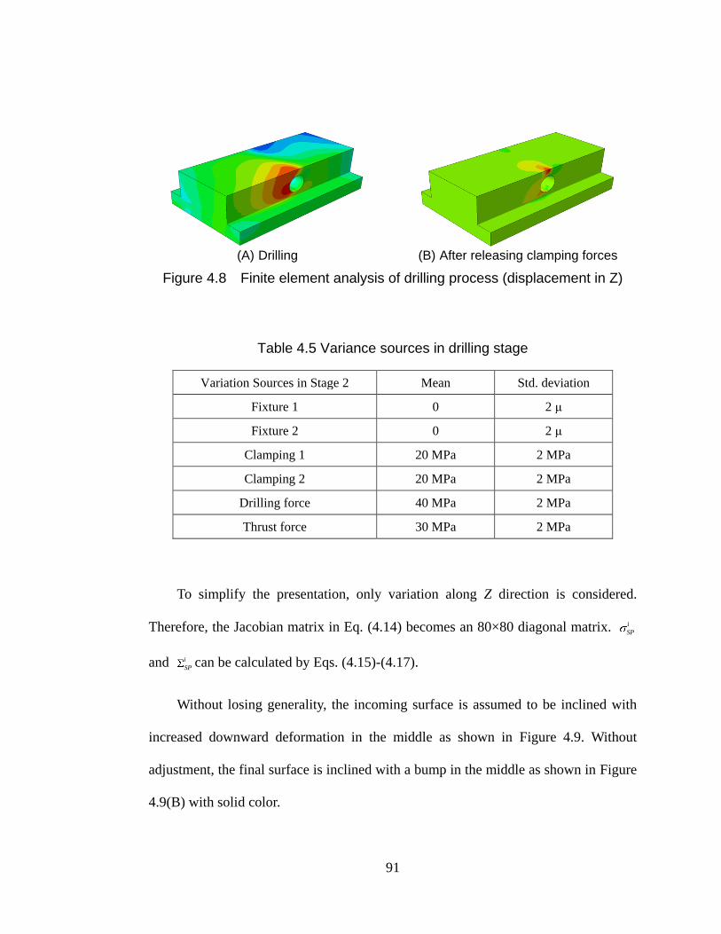
91
(A) Drilling (B) After releasing clamping forces
Figure 4.8 Finite element analysis of drilling process (displacement in Z)
Table 4.5 Variance sources in drilling stage
Variation Sources in Stage 2 Mean Std. deviation
Fixture 1 0 2 μ
Fixture 2 0 2 μ
Clamping 1 20 MPa 2 MPa
Clamping 2 20 MPa 2 MPa
Drilling force 40 MPa 2 MPa
Thrust force 30 MPa 2 MPa
To simplify the presentation, only variation along Z direction is considered.
Therefore, the Jacobian matrix in Eq. (4.14) becomes an 80×80 diagonal matrix. i
SP
and i
SPcan be calculated by Eqs. (4.15)-(4.17).
Without losing generality, the incoming surface is assumed to be inclined with
increased downward deformation in the middle as shown in Figure 4.9. Without
adjustment, the final surface is inclined with a bump in the middle as shown in Figure
4.9(B) with solid color.
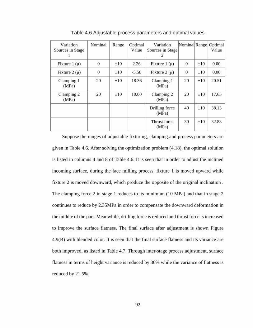
92
Table 4.6 Adjustable process parameters and optimal values
Variation
Sources in Stage
1
Nominal Range Optimal
Value
Variation
Sources in Stage
2
Nominal Range Optimal
Value
Fixture 1 (μ) 0 ±10 2.26 Fixture 1 (μ) 0 ±10 0.00
Fixture 2 (μ) 0 ±10 -5.58 Fixture 2 (μ) 0 ±10 0.00
Clamping 1
(MPa)
20 ±10 18.36 Clamping 1
(MPa)
20 ±10 20.51
Clamping 2
(MPa)
20 ±10 10.00 Clamping 2
(MPa)
20 ±10 17.65
Drilling force
(MPa)
40 ±10 38.13
Thrust force
(MPa)
30 ±10 32.83
Suppose the ranges of adjustable fixturing, clamping and process parameters are
given in Table 4.6. After solving the optimization problem (4.18), the optimal solution
is listed in columns 4 and 8 of Table 4.6. It is seen that in order to adjust the inclined
incoming surface, during the face milling process, fixture 1 is moved upward while
fixture 2 is moved downward, which produce the opposite of the original inclination .
The clamping force 2 in stage 1 reduces to its minimum (10 MPa) and that in stage 2
continues to reduce by 2.35MPa in order to compensate the downward deformation in
the middle of the part. Meanwhile, drilling force is reduced and thrust force is increased
to improve the surface flatness. The final surface after adjustment is shown Figure
4.9(B) with blended color. It is seen that the final surface flatness and its variance are
both improved, as listed in Table 4.7. Through inter-stage process adjustment, surface
flatness in terms of height variance is reduced by 36% while the variance of flatness is
reduced by 21.5%.

93
(A) Incoming surface (B) Final surfaces with (blended
color) and without (solid color) compensation
Figure 4.9 Case study on inter-stage form error compensation
Table 4.7 Comparison of surface flatness with and without compensation
Without error-compensation With error-compensation
Surface flatness 0.03431 0.02195
Sum of Variance 2.586×10⁻⁴
2.030×10⁻⁴
4.4.4. Backward Morphing Based Process Monitoring
This section demonstrates process monitoring through backward mapping and
multivariate control chart. 100 parts are simulated using the optimized process
parameters listed in Table 4.4 and Table 4.5 to estimate the between-part variation.
Principal component analysis is performed on the surface data and a scree plot is shown
in Figure 4.10. It is seen that the surface data are highly correlated since the first 3
principal components (PCs) capture over 99% of the total variation.
-50
0
50
100
150
010
2030
4050
0
0.01
0.02
0.03
0.04
-50
0
50
100
150
-100102030
4050
0
0.01
0.02
0.03
0.04

94
Figure 4.10 Scree plot of 100 training data
Figure 4.11 Phase I Hotelling’s T2 control chart at final stage
Assuming multivariate normality, Hotelling‟s T2 control charts based on the 3
PC‟s are constructed to monitor the backward morphed surfaces at intermediate stages.
The phase I control chart constructed by the 100 surfaces is shown in Figure 4.11.
Figure 4.12 shows the control charts for stages 0 and 1. It should be noted that both
control charts in Figure 4.12 are similar because clamping release at stage 1 has minor
impact on surface change (Figure 4.6).
(A) Control chart of stage 1 (B) Control chart of stage 0
Figure 4.12 Phase I Hotelling’s T2 control chart at prior stages
Phase II control chart is constructed to monitor 10 more surfaces that are
manipulated by adding inclining trend to parts as shown in Figure 4.13 (A). In Figure
4.13(B-D) all three T2 control charts shows out-of-control with linear trends.
1 2 3 4 50
0.2
0.4
0.6
0.8
1
Principle Component
Perc
enta
ge o
f Varia
nce
0 20 40 60 80 1000
2
4
6
8
10
Surface number
T2
sta
tistic
s
0 20 40 60 80 1000
2
4
6
8
10
Surface number
T2
sta
tistic
s
0 20 40 60 80 1000
2
4
6
8
10
Surface number
T2
sta
tistic
s
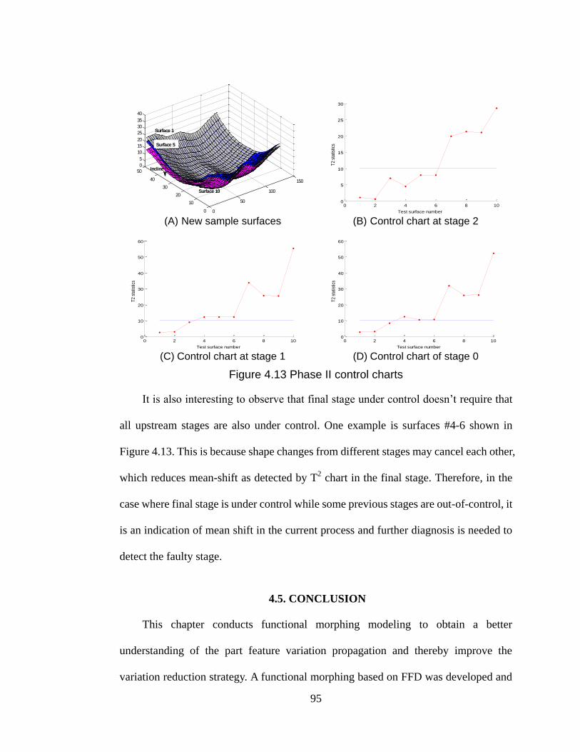
95
(A) New sample surfaces (B) Control chart at stage 2
(C) Control chart at stage 1 (D) Control chart of stage 0
Figure 4.13 Phase II control charts
It is also interesting to observe that final stage under control doesn‟t require that
all upstream stages are also under control. One example is surfaces #4-6 shown in
Figure 4.13. This is because shape changes from different stages may cancel each other,
which reduces mean-shift as detected by T2 chart in the final stage. Therefore, in the
case where final stage is under control while some previous stages are out-of-control, it
is an indication of mean shift in the current process and further diagnosis is needed to
detect the faulty stage.
4.5. CONCLUSION
This chapter conducts functional morphing modeling to obtain a better
understanding of the part feature variation propagation and thereby improve the
variation reduction strategy. A functional morphing based on FFD was developed and
0
50
100
150
0
10
20
30
40
50
0
5
10
15
20
25
30
35
40
Surface 5
Surface 10
Surface 1
Incline
0 2 4 6 8 100
5
10
15
20
25
30
Test surface number
T2
stat
istic
s
0 2 4 6 8 100
10
20
30
40
50
60
Test surface number
T2
stat
istic
s
0 2 4 6 8 100
10
20
30
40
50
60
Test surface number
T2
stat
istic
s

96
represented by forward and backward mapping functions that capture feature changes
as reflected from HDM data. Based on the established mapping functions, an
inter-stage process adjustment method was developed to compensate for the form
errors occurring at downstream stages. The repeatability of the adjustment strategy was
ensured by a backward-morphing based monitoring scheme. The morphing functions
in the adjustment algorithm need to be updated once an out-of-control signal indicates a
process change. A case study based on a cutting experiment along with simulation
demonstrated that the closed-loop adjustment strategy efficiently improved surface
flatness.
Compared with the conventional research on variation propagation, the
advantages of functional morphing for process control can be summarized as follows:
Improved geometry and texture characterization The FFD based functional
morphing can better describe the multi-scale feature changes (e.g., global shape,
local deformation or waviness.) as well as their variations. Such changes can take
place within each scale and potentially between scales. Thus, this approach will
lead to a multi-scale variation propagation analysis that incorporates more variation
sources for process control.
Incorporation of part physical properties The impact of part physical properties on
the surface feature change was considered via a bending energy term when deriving
the mapping functions. It should be noted that the physical properties can be
space-varying and time-varying. The functional morphing method therefore
provides the opportunities of utilizing heterogeneous physical properties (e.g.,

97
distributions of mass density or casting pore density) for variation control in
multistage precision machining.
Improved characterization of form error cancellation The cancellation among
complex form errors at different stages can be accurately acquired via morphing,
which enables an inter-stage process monitoring and adjustment.
High efficiency in dealing with HDM data The functional morphing methodology
facilitates the HDM data analysis efficiently since it defines a FFD volume space
on a sparse lattice and the volume space deforms between stages thereby avoiding
dealing with dense HDM data directly. This approach will improve computational
efficiency while satisfying both geometric constraint and physical feasibility.
REFERENCES
Apley, D. and Shi, J., (2001), “A Factor-Analysis Method for Diagnosing Variability in
Multivariate Manufacturing Processes”, Technometrics, Vol. 43, pp. 84-95.
Bookstein, F. L., (1989), “Principal Warps: Thin-Plate Splines and the Decomposition
of Deformations”, IEEE Transactions on Pattern Analysis and Machine
Intelligence, Vol. 11, pp. 567-585.
Cai, W., Hu, S.J. and Yuan, J., (1996), “A Variational Method of Robust Fixture
Configuration Design for 3-D Workpiece”, ASME Transactions: Journal of
Manufacturing Science and Engineering, Vol. 119, pp. 593-602.
Camelio, J., Hu, S.J. and Ceglarek, D., (2003), “Modeling Variation Propagation of
Multi-Station Assembly Systems with Compliant Parts”, ASME Transactions:
Journal of Mechanical Design, Vol. 125, pp. 673-681.
Coquillart, S., (1990), “Extended Free-form Deformation: A Sculpturing Tool for 3D
Geometric Modeling”, ACM SIGGRAPH Computer Graphics, Vol. 24, pp.
187-196.
Ding, Y., Ceglarek, D. and Shi, J., (2002), “Fault Diagnosis of Multistage
Manufacturing Processes by Using State Space Approach”, ASME
Transactions: Journal of Manufacturing Science and Engineering, Vol. 124 (2),
pp. 313-322.

98
Ding, Y., Jin, J., Ceglarek, D. and Shi, J., (2005), “Process-Oriented Tolerancing for
Multi-Station Assembly Systems”, IIE Transactions, Vol. 37, pp. 493-508.
Djurdjanovic, D. and Ni, J., (2001), “Linear State Space Modeling of Dimensional
Machining Errors”, Transactions of NAMRI/SME, Vol. 29, pp.541-548.
Hearn, D. and Baker, M.P., (1994), Computer Graphics, 2nd Edn., Prentice Hall, New
York.
Huang, Q. and Shi, J., (2003), “Simultaneous Tolerance Synthesis through Variation
Propagation Modeling of Multistage Manufacturing Processes”, Transactions
of NAMRI/SME, Vol. 31, pp. 515-522.
Huang, Q., Shi, J. and Yuan, J., (2003), “Part Dimensional Error and its Propagation
Modeling in Multi-Stage Machining Processes”, ASME Transactions: Journal
of Manufacturing Science and Engineering, Vol. 125, pp. 255-262.
Jin, J. and Shi, J., (1999), “State Space Modeling of Sheet Metal Assembly for
Dimensional Control,” ASME Transactions: Journal of Manufacturing Science
and Engineering, Vol. 121, pp. 756-762.
Keim, D. A. and Herrmann, A., (1998), “The Gridfit Algorithm: An Efficient and
Effective Approach to Visualizing Large Amounts of Spatial Data”, IEEE
Visualization: Proceedings of the Conference on Visualization, pp. 181-188.
Liu, J., Shi, J. and Hu, S.J., (2008) “Engineering-Driven Factor Analysis for Variation
Sources Identification in Multistage Manufacturing Processes”, ASME
Transactions: Journal of Manufacturing Science and Engineering, Vol. 130, pp.
0410091-10.
Mantripragada, R. and Whitney, D.E., (1999), “Modeling and Controlling Variation
Propagation in Mechanical Assemblies Using State Transition Models”, IEEE
Transactions on Robotics and Automation, Vol. 15, pp. 124-140.
Sederberg, T. W., and Parry, S. R., (1986), “Free-form Deformation of Polygonal Data”,
Proceedings of International Electronic Image Week, Nice, France pp. 633-639.
Shi, J., (2006), “Stream of Variation Modeling and Analysis for Multistage
Manufacturing Processes”, CRC Press, Taylor & Francis Group.
Taguchi, G., (1986), Introduction to Quality Engineering, Asian Productivity
Organization, Tokyo, Japan.
Ventsel, E. and Krauthammer, T., (2001), “Thin Plates and Shells: Theory, Analysis,
and Applications”, Marcel Dekker, New York.
Wang, H. and Huang, Q., (2007), “Using Error Equivalence Concept to Automatically
Adjust Discrete Manufacturing Processes for Dimensional Variation
99
Reduction", ASME Transactions: Journal of Manufacturing Science and
Engineering, Vol. 129, pp. 644-652.
Wu, C. F. J. and Hamada, M., (2000), “Experiments: Planning, Analysis, and Parameter
Design Optimization”, John Wiley and Sons Inc, New York.
Zhong, J., Liu, J. and Shi, J., (2009), “Predictive Control Considering Model
Uncertainty for Variation Reduction in Multistage Assembly Processes”, IEEE
Transactions on Automation Science and Engineering, Accepted as
TASE-2009-091.
Zhou, S., Chen, Y. and Shi, J., (2004), "Statistical Estimation and Testing for Variation
Root-Cause Identification of Multistage Manufacturing Processes", IEEE
transactions on Robotics and Automation, Vol. 1, pp.73-83.
Zhou, S., Huang, Q. and Shi, J., (2003), “State Space Modeling for Dimensional
Monitoring of Multistage Machining Process Using Differential Motion
Vector”, IEEE Transactions on Robotics and Automation, Vol. 19 (2), pp.
296-309.

100
CHAPTER 5
CONCLUSIONS AND FUTURE WORK
5.1. CONCLUSIONS
The research on functional morphing for manufacturing process design,
evaluation and control originates from the rapidly changing market requirement to
shorten product development time, as well as the constant need for manufacturing
process monitoring and control. Since shape change is an important goal of most
manufacturing processes, one potential solution facilitating process development is to
describe the shape changes using morphing, which has been widely utilized in the areas
of computer graphics, filming and medical imaging. However, current morphing
techniques are geometry driven without considering physical feasibility. Hence there
are limitations when these morphing techniques are used to characterize physical
processes. Therefore, a functional morphing concept has been proposed by
incorporating material and process considerations into geometric morphing. This
dissertation is aimed to develop functional morphing algorithms for manufacturing
process design and control. The developed methodologies enable an effective process
design and evaluation for evolutionary product development through functional
morphing between product generations. Meanwhile, these methodologies can also be
101
utilized for high-definition metrology based monitoring and control of multi-stage
manufacturing systems.
The major achievements of this dissertation can be summarized in three parts:
1) Development of a functional morphing methodology for stamping die face
design of evolutionary products: A new concept using functional
morphing for evolutionary die development has been proposed using three
sequential steps: part-to-part mapping between the existing part and the
new part, die-to-die morphing using the same parts mapping function, and
finite element verification. The mapping function is constructed by
functional morphing combining both geometric relationship between part
surfaces and a smoothness function which inherits the springback
compensation information. Results show that the morphed new die can
capture the difference of product design through generations as well as
springback compensation from previous die design. This study is
beneficial to die development of new product in the same product family
or different generations utilizing the existing product and die information.
2) Development of a functional morphing based strain increment method for
formability assessment in die face morphing: Based on the die face
morphing algorithm, a strain increment method has been introduced to
quickly predict the strain and evaluate the formability for a new part
generation. This method calculates the strain increment associated with
functional morphing between parts by introducing a bending energy and a
strain gradient penalty term. By superposition of the strain increment to

102
the original strain from the existing part, the strain field on the new part
can be estimated. Since this method does not require the knowledge on
new die surface, such formability assessment can be used as an early
feasibility assessment of the new part design.
3) Investigation of functional morphing in process control for multi-stage
manufacturing processes: A functional morphing model is developed to
investigate the part feature variation propagation for high-definition
metrology data through a multi-stage manufacturing process and thereby
improve the variation reduction strategy. This functional morphing
incorporates heterogeneous material properties such as density
distribution and is represented by forward and backward mapping
functions. Based on the established mapping function, this study also
develops an inter-stage process adjustment method to compensate for the
form errors occurring at downstream stages. And the repeatability of the
adjustment strategy is ensured by a backward-morphing based monitoring
scheme.
The original contributions of this research can be summarized as follows:
1) A new concept of functional morphing is introduced by incorporating
material and process information into the part geometry morphing. As
such functional morphing can better describe the physical changes in
manufacturing processes.
2) The concept of die face morphing is introduced to integrate the existing
die information into new die design for evolutionary product development.

103
Guidelines are proposed by using functional morphing based part-to-part
mapping, die-to-die morphing and finite element verification. It is found
that the morphed new die is able to capture the springback compensation
from the existing die by including a smoothness function in part-to-part
mapping and thus reduce the design-engineering iteration.
3) A strain increment method is developed to quickly assess the formability
of the new part using the geometric and strain information of its previous
generation. Functional morphing including a bending energy and a strain
gradient constraint is introduced to morph between part generations. It is
found that the predicted strain distribution is well compared with that from
finite element analysis.
4) The free-form deformation based functional morphing is developed to
describe feature changes as well as their variations through multi-stage
process. This approach can also lead to a multi-scale variation propagation
analysis that incorporates more variation sources for process control. The
cancellation among complex form errors at different stages is accurately
acquired via morphing, which enables an inter-stage process monitoring
and adjustment.
5) The functional morphing methodology is shown to improve computational
efficiency while satisfying both geometric constraint and physical
feasibility for the HDM data analysis.

104
5.2. FUTURE WORK
The methodologies and models proposed in this research could be further
improved and /or extended in the following directions:
1) The die face morphing method can be further extended to other
manufacturing processes designs for evolutionary products. For example,
in machining process, tool path can be morphed from existing product to
new product generation. In chemical mechanical polishing (CMP) process,
wafer topography can be morphed from one product to another to quickly
determine the process parameter adjustments.
2) The strain increment method can be improved by considering material
flow and complex boundary conditions. In sheet metal stamping, the
change of draw bead or blank holding force will affect material flows. The
strain increment method can incorporate these changes by transforming
them into equivalent constraints in functional morphing. Then, strain
distribution under these complex boundary conditions and material flows
can be estimated.
3) Formability estimation can be integrated into the die face morphing
algorithm for better determination of the new generation stamping die.
Formability is first estimated using the strain increment method combined
with strain or stress based approaches. During die face morphing, the
feasible solution region is further reduced by integrating the formability,
resulting in a better die face considering both springback compensation
and formability of the produced part.
105
4) The functional morphing modeling for multi-stage machining process can
be extended to multi-scale morphing, where the impact of one scale (e.g.,
global shape) can be morphed from other scales (e.g., localized features)
and vice versa. This can be done through morphing extrapolation from
small scale to large scale, or multi-level morphing from large scale to
small scale. Corresponding diagnosis and control strategies can be
developed for multi-stage multi-scale process monitoring and control.
5) The morphing based process control for multi-stage processes can be
extended to other manufacturing processes, such as multi-stage stamping
process including blanking, stamping, re-strikes, trimming, flanging and
hemming. Sheet metal products in the multi-stage stamping process can be
morphed through each operation. The developed inter-stage form error
compensation and monitoring methodologies can be utilized to adjust
these operations to compensate springback and reduce final product
variability.