fundamental mathematical techniques reviewed · fundamental mathematical techniques reviewed: ......

Fundamental mathematical techniques reviewed: • Mathematical induction • Recursion Typically taught in courses such as Calculus and Discrete Mathematics. Techniques introduced: • Divide-and-Conquer

Algorithms Covered: • Binary Search • Merge Sort

Russ Miller & Laurence Boxer Algorithms Sequential & Parallel: A Unified Approach, 3E Chapter 2 / Slide 1

Solutions From Simpler Cases

• Mathematical induction is a technique for proving statements about sets of consecutive integers. One can view this as being done by inducing our knowledge of the next case from that of its predecessor.

• Recursion is a technique where a solution to a problem consists of utilizing solutions to smaller versions of the problem.

• Divide-and-Conquer is a recursive technique:

i. Divide a large problem into smaller subproblems.

ii. Solve the subproblems recursively, unless the problems are small enough to be solved directly.

iii. Combine the solutions to the subproblems in order to obtain a solution to the original problem.


Mathematical Induction

• Given a statement about positive integers, show that the statement is always true.

• Let 𝑃(𝑛) be a predicate, a statement that is true or false, depending on its argument 𝑛. Assume 𝑛 is a positive integer.

• Example of Predicate: “The product of the positive integers from 1 to 𝑛 is divisible by 10.” • This predicate is true for 𝑛 = 5 since 1 × 2 × 3 × 4 × 5 = 120, which

is divisible by 10.

• This predicate is false for 𝑛 = 4 since 1 × 2 × 3 × 4 = 24, which is not divisible by 10.


Principle of Mathematical Induction

Given a predicate that it is true for all positive integers 𝑛, the predicate can typically be proved as follows.

• Let 𝑃(𝑛) be a predicate, where n is an arbitrary positive integer. Suppose the following can be accomplished.

1. Show that 𝑃(1) is true.

2. Show that whenever 𝑃(𝑘) is true, we can derive that 𝑃(𝑘 + 1) is also true.

• If these two goals can be achieved, then it follows that 𝑃(𝑛) is true for all positive integers n.


Why Does Mathematical Induction Work?

• Suppose the two steps on the previous slide have been proven.

• Then from step 1, 𝑃(1) is true, and thus by step 2, 𝑃 1 + 1 = 𝑃(2) is true, and thus by step 2, 𝑃 2 + 1 = 𝑃(3) is true, and thus by step 2, 𝑃 3 + 1 = 𝑃(4) is true, and so forth.

• That is, step 2 allows for the induction of the truth of 𝑃(𝑛) for every positive integer 𝑛 from the truth of 𝑃(1).

• Base Case: The statement 𝑃 1 = 𝑡𝑟𝑢𝑒 is referred to as the base case of the problem being considered.

• Inductive Hypothesis: The assumption in Step 2 that 𝑃 𝑘 = 𝑡𝑟𝑢𝑒 is called the Inductive Hypothesis. This is due to the fact that Step 2 is typically used to induce the conclusion that the statement 𝑃 𝑘 + 1 = 𝑡𝑟𝑢𝑒.


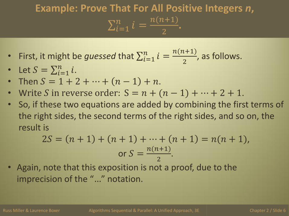
Example: Prove That For All Positive Integers n,

𝑖𝑛𝑖=1 =

𝑛(𝑛+1)

2.

Russ Miller & Laurence Boxer Algorithms Sequential & Parallel: A Unified Approach, 3E

• First, it might be guessed that 𝑖𝑛𝑖=1 =

𝑛(𝑛+1)

2, as follows.

• Let 𝑆 = 𝑖𝑛𝑖=1 .

• Then 𝑆 = 1 + 2 + ⋯+ 𝑛 − 1 + 𝑛. • Write 𝑆 in reverse order: S = 𝑛 + (𝑛 − 1) + ⋯+ 2 + 1. • So, if these two equations are added by combining the first terms of

the right sides, the second terms of the right sides, and so on, the result is

2𝑆 = 𝑛 + 1 + 𝑛 + 1 + ⋯+ 𝑛 + 1 = 𝑛(𝑛 + 1),

or 𝑆 =𝑛(𝑛+1)

2.

• Again, note that this exposition is not a proof, due to the imprecision of the “…” notation.

Chapter 2 / Slide 6

(continued)

Now, a formal proof is given of 𝑖𝑛𝑖=1 =

𝑛(𝑛+1)

2.

• The equation claims that the sum of the first 𝑛 positive

integers is 𝑛(𝑛+1)

2.

• Base case: For 𝑛 = 1, the left side of the asserted equation is 𝑖1

𝑖=1 = 1 and the right side of the asserted equation is 1(1+1)

2= 1.

• Thus, for 𝑛 = 1, the asserted equation is true. Therefore, the base case of the induction proof is achieved.


(continued)

• Inductive case: Suppose the asserted equation is valid for 𝑛 = 𝑘, for some positive integer 𝑘. Notice that it is justifiable to state this assumption due to the demonstration above that the case 𝑛 = 𝑘 = 1 is an instance for which the assumption is valid.

• Now, the asserted equation must be proven true for the next case, namely, 𝑛 = 𝑘 + 1. That is, by using the assumption for 𝑛 = 𝑘, it must be proven that

𝑖𝑘+1𝑖=1 =

(𝑘+1)(𝑘+2)

2.

• Notice that the left side of the latter equation can be rewritten as

𝑖𝑘+1𝑖=1 = 𝑖𝑘

𝑖=1 + (𝑘 + 1). • Substituting from the inductive hypothesis gives

𝑖𝑘+1𝑖=1 =

𝑘(𝑘+1)

2+ (𝑘 + 1) =

(𝑘+1)(𝑘+2)

2,

as desired. Thus, the proof is complete.


Recursion

• A subprogram that calls upon itself, either directly or indirectly, is called recursive. Formally, an algorithm exhibits recursive behavior when it can be defined by two properties.

• A simple base case or cases.

• A set of rules that reduce all other cases towards the base case.

• Recursive calls are made with a smaller/simpler set of data.

• When a call is made with a sufficiently small/simple enough set of data, the call is resolved directly.

• Notice the similarity of mathematical induction and recursion.

• Just as mathematical induction is a technique for inducing conclusions for “large n” from our knowledge of “small n,” recursion allows for the processing of large or complex data sets based on the ability to process smaller or less complex data sets.


Recursively Defined Factorial Function

Definition of n!: Let 𝑛 be a nonnegative integer. Then 𝑛! is defined as

𝑛! = 1 if 𝑛 = 0;

𝑛 × 𝑛 − 1 ! otherwise.

• Theorem: For 𝑛 > 0, 𝑛! is the product of the integers from 1 to 𝑛.

• So, 𝑛! can be computed using a tight loop.

• Note that the definition of 𝑛! is recursive and lends itself to a recursive calculation.


Example: Compute 3!

The definition of 𝑛! is used to compute 3! as follows.

• From the recursive definition, 3! = 3 × 2!.

• Thus, the value of 2! needs to be determined.

• Using the second line of the recursive definition, 3! = 3 ×2! = 3 × 2 × 1! = 3 × 2 × 1 × 0!.

• Notice that the first line of the Definition of n Factorial yields 0! = 1.

• This is the simplest case of 𝑛 considered by the definition of 𝑛!, a case that does not require further use of recursion and therefore is a base case.


Example: Compute 3! (continued)

A recursive definition or algorithm may have more than one base case. It is the existence of one or more base cases, and logic that drives the computation toward base cases, that prevent recursion from producing an infinite loop.

In the example, substitute 1 for 0! in order to resolve our calculations. If one were to proceed in the typical fashion of a person calculating with pencil and paper, this would yield

3! = 3 × 2 × 1 × 0! = 3 × 2 × 1 × 1 = 6.


Pseudocode for 𝑛!

Integer function factorial (integer 𝑛)

Input: 𝑛 is assumed to be a nonnegative integer.

Algorithm: Produce the value of n! by using recursion.

Action:

If 𝑛 = 0, then return 1

Else return 𝑛 × 𝑓𝑎𝑐𝑡𝑜𝑟𝑖𝑎𝑙 𝑛 − 1

- - - - - - - - - - - - - - - - - - - - - - - - - - - - - - - - - - - - - - - - - - - - -

How does one analyze the running time of this function?


Analysis of Factorial Function

• Let 𝑇(𝑛) denote the running time of the procedure with input value 𝑛.

• From the base case of the recursion, 𝑇 0 = Θ(1), since the time to compute 0! is constant.

• From the recurrence given above, the time to compute 𝑛!, for 𝑛 > 0, can be defined as 𝑇 𝑛 = 𝑇 𝑛 − 1 + Θ(1).

• The conditions

𝑇 0 = Θ(1);

𝑇 𝑛 = 𝑇 𝑛 − 1 + Θ 1 (1)

form a recursive relation.

• Now, evaluate 𝑇(𝑛) in such a way as to express 𝑇(𝑛) without recursion.


Analysis of Factorial Function (continued)

• Repeated substitution of the recursive relation results in 𝑇 𝑛 = 𝑇 𝑛 − 1 + Θ 1 =

𝑇 𝑛 − 2 + Θ 1 + Θ 1 = 𝑇 𝑛 − 2 + 2Θ 1 =

𝑇 𝑛 − 3 + Θ 1 + 2Θ 1 = 𝑇 𝑛 − 3 + 3Θ 1 .

• The emerging pattern is

𝑇 𝑛 = 𝑇 𝑛 − 𝑘 + 𝑘Θ 1 .

• Such a pattern will lead us to conjecture that

𝑇 𝑛 = 𝑇 0 + 𝑛Θ 1 ,

which, by the base case of the recursive definition, yields

𝑇 𝑛 = Θ 1 + 𝑛Θ 1 = Θ 𝑛 .

• Note the above is not a proof.


Analysis of factorial function (continued)

Observe that the Θ-notation in condition (1) is a generalization of proportionality. Suppose the simplified recursive relation is considered

𝑇 0 = 1;𝑇 𝑛 = 𝑇 𝑛 − 1 + 1.

(2)

Previous observations leads one to suspect that this yields 𝑇 𝑛 = 𝑛 + 1. A proof by mathematical induction follows.

• For 𝑛 = 0, the assertion is 𝑇 0 = 1, which is true.


Analysis of factorial function (continued)

• Suppose the assertion is true for some nonnegative integer k. Thus, the inductive hypothesis is the equation 𝑇 𝑘 = 𝑘 + 1.

• Now, one needs to show 𝑇 𝑘 + 1 = 𝑘 + 2. Using the recursive relation (2) and the inductive hypothesis yields 𝑇 𝑘 + 1 = 𝑇 𝑘 + 1 = 𝑘 + 1 +1 = 𝑘 + 2, as desired.

• Since condition (1) is a generalization of (2), in which the Θ-interpretation is not affected by the differences between (1) and (2), it follows that condition (1) satisfies 𝑇 𝑛 = Θ(𝑛).


Computing Fibonacci Numbers

RecursiveFibonacci(n)

Input: a non-negative number n

Output: the Fibonacci number with index n

If n=0 then return 1

If n=1 then return 1

f =RecursiveFibonacci(n-1) + RecursiveFibonacci(n-2)

Return(f)


Recursion Tree


RF(5)

RF(4) RF(3)

RF(1)

RF(0)

RF(3) RF(2)

RF(1) RF(1) RF(2)

RF(2)

RF(1) RF(0)

RF(1) RF(0)

Sequential Search (Non-Recursive)

The traditional non-recursive sequential search algorithm is presented so that it can be compared to the recursive implementation of binary search that is given later.

Consider the problem of searching an unordered set of data by a traditional sequential search.

• In the worst case, every item must be examined, since the item being sought i) might not exist or ii) might be the last item listed.

• So, without loss of generality, it is assumed that the sequential search starts at the beginning of the unordered data set and concludes based on one of the following conditions.

• The search succeeds when the required item is located.

• The search fails after every item has been examined without finding the item being sought.


Sequential Search (continued)

Since the data is not known to be ordered, the sequential examination of data items is necessary. Note that if any data item is skipped, that item could be the one being sought.

Figure 2-1. An example of sequential search. Given the array of data, a search for the value 4 requires five key comparisons. A search for the value 9 requires three key comparisons. A search for the value 1 requires seven key comparisons in order to determine that the requested value is not present.


Subprogram SequentialSearch (X, searchValue, success, foundAt) (continued)

Action:

position = 1

Do

success = (searchValue = X[position])

If success, then foundAt = position

Else position = position + 1

While (Not success) and (position ≤ 𝑛 ) {End Do}

Return success, foundAt

End Search


Analysis of Sequential Search

• The set of instructions inside the loop runs in Θ 1 time since each instruction runs in Θ 1 time.

• In the worst case, the body of the loop will be executed 𝑛 times.

• This occurs when either the search is unsuccessful or when the item we seek is the last item in the array X.

• Thus, the worst-case sequential search runs in Θ 𝑛 time.

• Assuming that the data is ordered in a truly random fashion, then a successful search will, on average, succeed after examining half of the entries.

• So, the average successful search runs in Θ 𝑛 time.

• Finally, since the data is presented in a random fashion, it is possible that the item being sought is found immediately. So, the time required for the best-case search is Θ 1 .


Binary Search

• Recursion is commonly used when every recursive call involves a significant reduction in the size of the current instance of the problem.

• An example of such a recursive algorithm is Binary Search.

• Consider the impact of performing a search on a sorted set of data. Think about designing an algorithm that mimics what you would do to find “Miller” in a hardcopy phone book.

• That is, grab a bunch of pages and flip back and forth, each time grabbing fewer and fewer pages, until the desired item is located.

• Notice that this method considers very few data values relative to the number considered by a sequential search.


Subprogram BinarySearch(X, searchValue, success, foundAt, minIndex, maxIndex)

Algorithm: Binary search algorithm to search ordered subarray for a key field equal to searchValue.

The algorithm is recursive. In order to search the entire array, assuming indices 1,… , 𝑛, the initial call is of the form Search(X, searchValue, success, foundAt, 1, 𝑛).

If searchValue is found, return success = true and foundAt as an index at which searchValue is found; otherwise, return success = false.

Local variable: index midIndex

Action:

If minIndex > maxIndex, then {The subarray is empty}

success = false, foundAt = 0

Else {The subarray is nonempty}


BinarySearch Algorithm (continued)

midIndex = (minIndex + maxIndex) / 2 If searchValue = X[midIndex].key, then success = true, foundAt = midIndex Else {searchValue ≠ X[midIndex].key} If searchValue < X[midIndex].key, then BinarySearch(X, searchValue, success, foundAt, minIndex, midIndex - 1) Else { searchValue > X[midIndex].key} BinarySearch(X, searchValue, success, foundAt, midIndex + 1, maxIndex); End {Else searchValue ≠ X[midIndex].key} End {Subarray is nonempty} End Search


Examples of Binary Search

Figure 2-2. Given the array of data, a search for the value 4 requires two key comparisons (6,4). A search for the value 9 requires three key comparisons (6,8,9). A search for the value 1 requires three key comparisons (6,4,3) in order to determine that the value is not present.


Analysis of Binary Search

• Each recursive call processes an interval of about ½ the length of the interval processed by the previous call, so the running time, 𝑇(𝑛), of the binary search algorithm satisfies the recursive relation

𝑇 1 = Θ(1);

𝑇 𝑛 ≤ 𝑇𝑛

2+ Θ(1).

• Seeking a pattern: Notice in the worst case,

𝑇 𝑛 = 𝑇𝑛

2+ Θ 1 =

𝑇𝑛

4+ Θ 1 + Θ 1 = 𝑇

𝑛

4+ 2Θ 1 =

𝑇𝑛

8+ Θ 1 + 2Θ 1 = 𝑇

𝑛

8+ 3Θ 1 .

• It appears 𝑇 𝑛 = 𝑇 𝑛/2𝑘 + 𝑘Θ 1 , where the argument of

T reaches the base value 1 = 𝑛/2𝑘 when 2𝑘 = 𝑛, or 𝑘 = log2 𝑛. Such a pattern leads us to the conjecture that

𝑇 𝑛 = 𝑇 1 + log2 𝑛 × Θ 1 = Θ log 𝑛 .


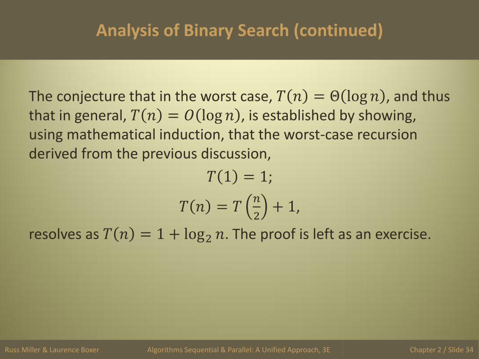
Analysis of Binary Search (continued)

The conjecture that in the worst case, 𝑇 𝑛 = Θ log 𝑛 , and thus that in general, 𝑇 𝑛 = 𝑂 log 𝑛 , is established by showing, using mathematical induction, that the worst-case recursion derived from the previous discussion,

𝑇 1 = 1;

𝑇 𝑛 = 𝑇𝑛

2+ 1,

resolves as 𝑇 𝑛 = 1 + log2 𝑛. The proof is left as an exercise.


Comparison of Sequential and Binary Searches

Sequential

search

Binary search

Data Not ordered Ordered by search

key

Time for search that fails Θ(𝑛) Θ(log 𝑛)

Worst-case time for search

that succeeds

Θ(𝑛) Θ(log 𝑛)

Expected-case time for

search that succeeds

Θ(𝑛) Θ(log 𝑛)

Best-case time for search

that succeeds

Θ(1) Θ(1)


Figure 2-3. Recursively sorting a set of data. Take the initial list and divide it into two lists, each roughly half the size of the original list. Recursively sort each of the sublists. Merge these sorted sublists to create the final sorted list.

Recursive Sorting Algorithms


Analyzing a Recursive Sorting Algorithm

The recursive relation that describes the running time of such an algorithm is given by

𝑇 1 = Θ 1 ; 𝑇 𝑛 = 𝑆 𝑛 + 2𝑇(𝑛 2) + 𝐶 𝑛 ,

where 𝑆 𝑛 is the time used by the algorithm to split a list of n entries into two sublists of approximately 𝑛/2 entries apiece, and 𝐶 𝑛 is the time used by the algorithm to combine two sorted lists of approximately 𝑛/2 entries apiece into a single sorted list. Discuss 𝑆 𝑛 = Θ(𝑛) since S = Split = Θ(𝑛) and C = Merge = Θ(𝑛)


Merge Sort: The Split Step


• Divide the input list X into 2 other lists Y and Z in a simple fashion. • A commonly used method: mimic how you might partition a deck

of cards into 2 piles of equal size. • Elements of X alternate between going into Y and going into Z. • E.g., a member whose initial rank in X is odd goes into Y and a

member whose initial rank in X is even goes into Z. • This is illustrated in Figure 2-3, above.

• Analysis: This step is essentially a scan of X, hence is performed in 𝑆 𝑛 = Θ(𝑛) time.

Chapter 2 / Slide 38

Merge Sort: The Combine Step


Combine step: since the recursive calls have produced Y and Z as sorted lists, merge these sorted lists into a sorted list X.

Figure 2-5. An example of merging two ordered lists, initially indexed by head1 and head2, to create an ordered list headMerge. Snapshots are presented at various stages of the algorithm. As the merge progresses, head1 and head2 each indexes the first unmerged node in their respective list.


Merging Two Lists


Input: lists Y and Z with a total of n members, each in ascending order Output: list X, initially empty, is output with members that were the input members of Y and Z , in ascending order Action: While Y and Z are both non-empty, do the following.

Compare the first members of Y and Z . Whichever has the smaller key value is removed from its list and placed at the end of X. Note one of Y and Z shrinks, and X grows. This is done in Θ(1) time.

End While. The time required for this loop is bounded above by 𝑂(𝑛) and below by the length of the shorter of the input lists. In a general merge, the best case runs in Θ(1) time. In Merge Sort, the input Y and Z have approximately 𝑛/2 members each. Thus, the loop runs in Θ(𝑛) time. Now, one of Y and Z is empty, and the other isn’t. Concatenate X and the non-empty one of Y and Z in Θ(1) time. Chapter 2 / Slide 40

Merge Sort: Analysis


• The running time of Merge Sort satisfies 𝑇 1 = Θ 1 ;

𝑇 𝑛 = 𝑆 𝑛 + 2𝑇(𝑛 2) + 𝐶 𝑛 , where the splitting time is 𝑆 𝑛 = Θ(𝑛) and the combine time is the time for a merge operation, 𝐶 𝑛 = Θ(𝑛).

• This yields 𝑇 1 = Θ 1 ;

𝑇 𝑛 = 2𝑇(𝑛 2) + Θ 𝑛 . • The recursive relation is resolved as

𝑇 1 = 1; 𝑇 𝑛 = 2𝑇(𝑛 2) + 𝑛 ,

by substituting 𝑛 = 2𝑘. This gives 𝑇 1 = 1;

𝑇 2𝑘 = 2𝑇 2𝑘−1 + 2𝑘.


} →Θ(n log n)

Merge Sort Analysis (continued)


• Using mathematical induction on k yields 𝑇 𝑛 = 𝑛 1 + log2 𝑛 .

The details of how this is done are left as an exercise. • Hence, Merge Sort runs in Θ 𝑛 log 𝑛 time.


fundamental mathematical techniques reviewed · fundamental mathematical techniques reviewed: ......

Documents