fundamental mathematical concepts for problems arising...
TRANSCRIPT

DIPLOMARBEIT
Titel der Diplomarbeit
“Fundamental Mathematical Conceptsfor Problems Arising in Robotics”
Verfasserin
Bettina Ponleitner
angestrebter akademischer Grad
Magistra der Naturwissenschaften (Mag.rer.nat)
Wien, im April 2013
Studienkennzahl lt. Studienblatt: A 405Studienrichtung lt. Studienblatt: MathematikBetreuer: ao. Univ.-Prof. Dipl.-Ing. Dr. Hermann Schichl

ii

Acknowledgements
First and foremost, my heartfelt and deepest thanks go to my family: to my par-ents Alice Stohl and Ulrich Ponleitner, who were throughout my studies alwaysencouraging and supporting me, and in particular, to my sister Nathalie Ponleit-ner, who provided me with invaluable advice and motivation, and always foundtime for talking with me–sometimes literally at night and day. Their absoluteand on-going belief in me and my abilities always have been and still are of greatsignificance to me. Further, I sincerely thank Tina Schrutka for her friendship, foralways listening to me, and if needed, for cheering me up. And, last but not least,I express my deep gratitude to my advisor Hermann Schichl, for his great support,patient guidance and enthusiastic inspiration.
iii

iv

Abstract
Robotics summarizes the aspects of designing, building and analyzing robots. Itposes a large number of challenging highly nonlinear, often algebraic problems ina moderate number of variables. Due to the nonlinearities the relevant (systemsof) equations usually have multiple solutions. Further, safety considerations orthe demand for a complete analysis require a worst case analysis of the possiblescenarios. Additionally, uncertainties like manufacturing tolerances on the me-chanical structure, sensor measurement errors, or numerical round-off errors haveto be taken into account.
A large number of research results is available in the field of robotics. This the-sis gives a survey of recent results concerning several geometrical and kinematicproblems (in particular for parallel robots), with emphasis on the mathematicaltools used for solving them. Due to the high interdisciplinary character of this re-search area, a wide variety of mathematical methods is used for solving the posedproblems, which cannot be covered here in total. Therefore, the mathematicalpart of the thesis is restricted to giving an overview of several methods for solvingsystems of nonlinear equations, and to outline main concepts of interval analysis.
v

vi

Zusammenfassung
Das Forschungsfeld der Robotik umfasst samtliche Aspekte, die die Entwicklung,Konstruktion und Analyse von Robotern betreffen. Es wirft eine Vielzahl vonanspruchsvollen Problemstellungen auf, die im Allgemeinen hochgradig nichtline-ar mit einer uberschaubaren Anzahl von Variablen sind. Aufgrund ihres nichtli-nearen Charakters haben die relevanten Gleichungen bzw. Gleichungssysteme imNormalfall mehrere Losungen. In vielen Fallen ist eine
”worst case“-Untersuchung
samtlicher moglicher Szenarien erforderlich, zum Beispiel wenn Sicherheitsaspektegepruft oder eine komplette Analyse des Problems durchgefuhrt werden sollen. Daes im realen Leben keinen idealen
”perfekten“ Roboter gibt, mussen zusatzlich
noch diverse Unsicherheitsfaktoren berucksichtigt werden, wie zum Beispiel Ferti-gungstoleranzen an der mechanischen Struktur eines Roboters, Sensor-Messfehleroder numerische Rundungsfehler.
Es gibt eine große Anzahl von Forschungspublikationen, die sich mit verschie-densten Fragestellungen der Robotik beschaftigen. Die vorliegende Arbeit gibteinen Uberblick uber Forschungsergebnisse der jungeren Vergangenheit, die sichauf verschiedene kinematische und Modellierungs-Problemstellungen beziehen, ins-besondere fur parallele Roboter. Dabei liegt der Fokus auf den mathematischenMethoden, die zur Losung herangezogen werden. Aufgrund des starken interdiszi-plinaren Charakters der Robotik sind die verwendeten mathematischen Technikensehr breit gefachert. Nachdem eine detaillierte Beschreibung samtlicher Methodenmehrere Bucher fullen wurde, beschrankt sich diese Arbeit darauf, einen Uberblickuber verschiedene Methoden zum Losen nichtlinearer Gleichungssysteme zu geben,und daruber hinaus wesentliche Konzepte der Intervall Analysis zu prasentieren.
vii

viii

Contents
Introduction 3
I Mathematical Methods 3
1 Solving Systems of Nonlinear Equations 5
1.1 Introduction . . . . . . . . . . . . . . . . . . . . . . . . . . . . . . . 5
1.2 Preleminaries . . . . . . . . . . . . . . . . . . . . . . . . . . . . . . 6
1.2.1 Polynomials . . . . . . . . . . . . . . . . . . . . . . . . . . . 6
1.2.2 Number of Solutions . . . . . . . . . . . . . . . . . . . . . . 7
1.3 Polynomial Continuation . . . . . . . . . . . . . . . . . . . . . . . . 8
1.4 Grobner Bases . . . . . . . . . . . . . . . . . . . . . . . . . . . . . . 13
1.5 Elimination . . . . . . . . . . . . . . . . . . . . . . . . . . . . . . . 17
2 Interval Analysis 23
2.1 Introduction . . . . . . . . . . . . . . . . . . . . . . . . . . . . . . . 23
2.2 Basic Properties of Interval Arithmetic . . . . . . . . . . . . . . . . 24
2.2.1 Intervals . . . . . . . . . . . . . . . . . . . . . . . . . . . . . 24
2.2.2 Rounded interval arithmetic . . . . . . . . . . . . . . . . . . 25
2.2.3 Boxes, interval vectors, and interval matrices . . . . . . . . . 26
2.2.4 Interval extensions of arithmetic expressions . . . . . . . . . 28
2.2.5 Enclosures for the range of a function . . . . . . . . . . . . . 29
2.3 Solving Linear Systems of Equations . . . . . . . . . . . . . . . . . 31
2.4 Solving Nonlinear Systems of Equations . . . . . . . . . . . . . . . 34
ix

x Contents
II Robotics 39
3 Architecture 41
3.1 Introduction . . . . . . . . . . . . . . . . . . . . . . . . . . . . . . . 41
3.2 General structure of robot mechanisms . . . . . . . . . . . . . . . . 41
3.3 Description of open-loop kinematic chains . . . . . . . . . . . . . . 45
3.3.1 Denavit-Hartenberg parameters . . . . . . . . . . . . . . . . 46
3.3.2 Screw displacements . . . . . . . . . . . . . . . . . . . . . . 50
3.4 Separable (parallel) robots . . . . . . . . . . . . . . . . . . . . . . . 51
4 Geometry 55
4.1 Introduction . . . . . . . . . . . . . . . . . . . . . . . . . . . . . . . 55
4.2 Sets and Maps . . . . . . . . . . . . . . . . . . . . . . . . . . . . . . 56
4.3 Generalized coordinates . . . . . . . . . . . . . . . . . . . . . . . . 57
4.4 Workspace . . . . . . . . . . . . . . . . . . . . . . . . . . . . . . . . 60
4.4.1 Workspace for parallel robots . . . . . . . . . . . . . . . . . 63
4.4.2 Workspace for serial manipulators . . . . . . . . . . . . . . . 66
4.4.3 Related problems . . . . . . . . . . . . . . . . . . . . . . . . 67
5 Geometric Kinematics: Forward and Inverse Kinematics 69
5.1 Introduction . . . . . . . . . . . . . . . . . . . . . . . . . . . . . . . 69
5.2 Serial Manipulators . . . . . . . . . . . . . . . . . . . . . . . . . . . 70
5.3 Parallel manipulators . . . . . . . . . . . . . . . . . . . . . . . . . . 73
5.3.1 Inverse kinematics of parallel manipulators . . . . . . . . . . 73
5.3.2 Direct kinematics of parallel manipulators . . . . . . . . . . 75
6 Differential kinematics 87
6.1 Introduction . . . . . . . . . . . . . . . . . . . . . . . . . . . . . . . 87
6.2 Velocity . . . . . . . . . . . . . . . . . . . . . . . . . . . . . . . . . 87
6.3 Jacobian and inverse Jacobian matrix . . . . . . . . . . . . . . . . . 89

Contents xi
6.3.1 Formulation of the (inverse) Jacobian of parallel robots . . . 90
6.3.2 Tasks . . . . . . . . . . . . . . . . . . . . . . . . . . . . . . . 93
6.4 Acceleration . . . . . . . . . . . . . . . . . . . . . . . . . . . . . . . 94
7 Dexterity and Error Bounds 97
7.1 Introduction . . . . . . . . . . . . . . . . . . . . . . . . . . . . . . . 97
7.2 Modelling the accuracy of a pose . . . . . . . . . . . . . . . . . . . 98
7.3 Dexterity indices . . . . . . . . . . . . . . . . . . . . . . . . . . . . 100
7.3.1 Error bounds depending on the norm . . . . . . . . . . . . . 101
7.3.2 The manipulability index . . . . . . . . . . . . . . . . . . . . 102
7.3.3 The condition number as error amplification factor . . . . . 102
7.3.4 Sensitivity indices . . . . . . . . . . . . . . . . . . . . . . . . 103
7.3.5 Global dexterity . . . . . . . . . . . . . . . . . . . . . . . . . 104
7.4 Errors and Global Optimization . . . . . . . . . . . . . . . . . . . . 105
8 Singularities 111
8.1 Introduction . . . . . . . . . . . . . . . . . . . . . . . . . . . . . . . 111
8.2 Singular configurations . . . . . . . . . . . . . . . . . . . . . . . . . 111
8.2.1 Singularities and velocities . . . . . . . . . . . . . . . . . . . 112
8.2.2 Singularities and forces . . . . . . . . . . . . . . . . . . . . . 113
8.2.3 Singularities and kinematics . . . . . . . . . . . . . . . . . . 113
8.3 Singularity Analysis . . . . . . . . . . . . . . . . . . . . . . . . . . . 114
8.3.1 Determination of the singularity-free workspace . . . . . . . 114
8.3.2 Singularity index . . . . . . . . . . . . . . . . . . . . . . . . 115
8.3.3 FKP and path planning . . . . . . . . . . . . . . . . . . . . 116
Conclusion 120
List of Figures 124

xii Contents
References 150
Curriculum Vitae 151

Introduction
Robotics summarizes the aspects of designing, building and analyzing robots. Itposes a large number of challenging highly nonlinear, often algebraic problems ina moderate number of variables. Due to the nonlinearities the relevant (systemsof) equations usually have multiple solutions. Further, safety considerations orthe demand for a complete analysis require a worst case analysis of the possiblescenarios. Therefore, the problems may be formulated as constraint satisfactionproblems or global optimization problems. Additionally, uncertainties like man-ufacturing tolerances on the mechanical structure, sensor measurement errors, ornumerical round-off errors have to be taken into account.
A large number of research results1 is available in the field of robotics. When werestrict our focus on the mechanical architecture of robots rather than on the ar-tificial intelligence aspect (therefore see, e.g., Russell & Norvig [267]), we canidentify two main classes of mechanical architectures: serial and parallel robots.This thesis gives a survey of recent results concerning geometrical and kinematicproblems arising in robotics. As parallel manipulators have become more and morepopular in the last two decades, and have taken the center stage in research, thefocus is laid on problems related to parallel robots. Since parallel robots may bedesigned in various different ways with specific properties, preferably results withgeneral character are presented here; in particular, so-called Gough-type manipu-lators are outlined, since these probably pose the most demanding problems in thefield. Thereby, the problems are looked at from a “mathematical” point of view,i.e., emphasis is placed on the formulation of the problems and the mathematicalmethods used for solving them. Robotics is a field with high interdisciplinary char-acter, and therefore, a wide variety of mathematical methods is used for solvingthe posed problems. Due to lack of space, only a few methods are outlined.
The goal of the thesis is to present several problems arising in robotics in sucha way, that they are accessible to a mathematician without specific engineeringknowledge, and further, to provide an overview of the major computational chal-lenges in the field, with the intention to pave the way for further research.
The thesis is organized as follows. Basically, it is divided in two main parts: Part Icovers fundamental mathematical concepts necessary for solving certain problems
1An extensive robotics bibliography library can be found at http://www-sop.inria.fr/members/Jean-Pierre.Merlet/references_robotique.html.
1

2 Introduction
arising in robotics; Part II then provides the contents particularly concerningrobotics.
In general, the kinematic analysis of robots relies on solving systems of nonlinear,and frequently algebraic equations. In Chapter 1 three different approaches arepresented, in particular polynomial continuation, Grobner bases and elimination,in order to provide a sufficient background on methods for achieving a solution ofsuch a system.
The methods discussed in the previous chapter may be insufficient, in particular,if all solutions of a certain problem are searched for, in the presence of uncer-tainties (such as round-off errors or measurement errors) or, if certified resultsare demanded. Therefore, in Chapter 2, main concepts of interval analysis areoutlined. Due to the specific structure of the field, the theory is introduced morethoroughly than the methods before.
In Chapter 3 the general structure of robot mechanisms is described, and basicdefinitions are given. Further, Denavit–Hartenberg parameters and screw displace-ments for the description of open-loop kinematic chains are introduced.
Chapter 4 deals with the geometry of robot manipulators. The notion of theequation of state is introduced and several sets and maps are defined, which areconvenient for formulating the main types of geometrical problems. Additionally,generalized coordinates are introduced and a parametrization in terms of quater-nions is presented. Finally, a description of several types of the workspace of arobot is given, as well as results concerning their determination.
A significant part of the kinematic analysis of a robot consists of deriving thesolution(s) of the forward and inverse kinematics problem, i.e., calculating thestate of a robot from measurements or poses. Therefore, Chapter 5 providesmain results about obtaining solutions to these problems.
Another main task of the kinematic analysis of a robot is to study the changesof geometry and the resulting translational and angular velocities and accelera-tions. Velocity, acceleration and the crucial notion of the kinematic Jacobian arediscussed in Chapter 6.
For applications it is important to know about the flexibility and accuracy withwhich the end-effector of a robot is placed in a given pose. Several methods havebeen proposed to quantify these features. So, in Chapter 7 an approach for themodeling of the accuracy of a pose, as well as a critical review of several dexterityindices are given. Additionally, the relationship between positioning errors and(global) optimization problems is summarized.
Finally, the singularity analysis of parallel robots is addressed in Chapter 8. Theconcept of singular configurations is considered briefly from different points ofview, and a summary of results concerning the determination of singularities isgiven.

Part I
Mathematical Methods
3


Chapter 1
Solving Systems of NonlinearEquations
1.1 Introduction
The kinematic analysis of a robotic manipulator usually depends on the solution ofsets of nonlinear equations. In Chapter 5 two basic problems where such systemsof nonlinear equations typically occur, the inverse kinematics problem for serialmanipulators and the forward kinematics problem of parallel manipulators, aredescribed. Furthermore, results concerning the number of (real) solutions and thespecific solutions are presented. There is a variety of both numerical and algebraictechniques available to solve such systems of equations and to give bounds onthe number of solutions. This chapter provides a summary of three often usedtechniques for solving algebraic systems, i.e., systems of polynomial equations
f(x) :=
f1(x1, . . . , xm)...
fn(x1, . . . , xm)
= 0, (1.1)
where f : Cm → Cn. The techniques presented are polynomial continuation,Grobner bases, and dialytic elimination. To begin with, some notation and re-marks about polynomials and the number of solutions are given.
5

6 Chapter 1. Solving Systems of Nonlinear Equations
1.2 Preleminaries
1.2.1 Polynomials
A polynomial f in variables x1, . . . , xn with coefficients aα ∈ K is a finite linearcombination of monomials, i.e.,
f =∑|α|≤m
aαxα,
where α = (α1, . . . , αm) is a multiindex with αi ≥ 0 for all i = 1, . . . ,m and
xα := xα11 x
α22 · · ·xαm
m .
The set of all polynomials in x1, . . . , xn and coefficients in a field K together withpointwise addition and multiplication is an integral domain, called the ring ofpolynomials, denoted by K[x1, . . . , xn]. The degree of each monomial is thesum of its exponents, i.e., |α| :=
∑i αi. For example, for f = 5x2
1 + 3x1x22 +x2− 3
the degrees of the monomials x21, x1x
22, and x2 are 2, 3, and 1, respectively. The
degree of the polynomial is equal to the degree of its highest degree term, whichis the so-called leading term, denoted by lt(f). The coefficient of the leadingterm of the polynomial is called the leading coefficient, denoted by lc(f). Theexpression power product refers to the monomials in a polynomial, e.g., forx3
1x2 + 4x21x3 + 2x3 + 1 = 0 the power products are x3
1x2, x21x3, x3, and 1. The
leading power product, denoted by lp(f), is the power product of the leadingterm of a polynomial; in the previous example, lp = x3
1x2.
The total degree of a system as in (1.1) is the product of the degrees of itsindividual polynomial equations [253].
Definition 1.2.1 (Affine variety). Let f1, . . . , fs be polynomials in K[x1, . . . , xn].Then
V (f1, . . . , fs) := (a1, . . . , an) ∈ Kn | fi(a1, . . . , an) = 0 ∀1 ≤ i ≤ n
is called the affine variety defined by f1, . . . , fs.
For example, f = x21 + x2
2 − x23 describes the cone, which is an affine variety given
by Vc := V (f) = (x1, x2, x3) ∈ Cn | x21 + x2
2 − x23 = 0. In particular, the set of
polynomials in (1.1) defines an affine variety.
Definition 1.2.2 (Ideal). A subset I ⊂ K[xa, . . . , xm] is an ideal if it satisfies
(i) 0 ∈ I,
(ii) if f, g ∈ I, then f + g ∈ I,
(iii) if f ∈ I and h ∈ K[x1, . . . , xm], then h · f ∈ I.

1.2. Preleminaries 7
E.g., for f = x21 +x2
2−x23 the set Ic = f, consisting of all polynomials vanishing
on Vc, is an ideal in the ring of polynomials C[x, y, z]. It can be shown that forf1, . . . , fs ∈ K[x1, . . . , xm],
〈f1, . . . , fn〉 :=∑s
i=1 hifi | h1, . . . , hn ∈ K[x1, . . . , xm]
is an ideal; 〈f1, . . . , fn〉 is said to be generated by f1, . . . , fn. For further informa-tion on varieties and ideals see, e.g., [56].
Definition 1.2.3 (Multiplicity [285]). The multiplicity µ(f, x∗) of an an isolatedsolution x∗ of (1.1) is defined as the dimension of the finite dimensional vectorspace
OCn,x∗/Ix∗ ,
where OCn,x∗ is the ring of convergent power series centered at x∗, and Ix∗ denotesthe ideal of OCn,x∗ generated by the polynomials f1, . . . , fn.
A solution x∗ being an isolated solution means that there are no other solutionsin the vicinity, i.e., the solution point x∗ does not belong to a higher dimensionalsolution set (such as a curve or a surface). For n = m = 1 this definition agreeswith the commonly used notion of multiplicity, i.e., given p(x) ∈ C[x], a notidentically zero polynomial in one variable, the multiplicity of a point x∗ ∈ V (p)is the integer µ > 0 such that p(x) = (x − x∗)µq(x) for a polynomial q(x) withq(x∗) 6= 0. In the case n = m > 1, µ has a simple geometrical interpretation. Ifx∗ is an isolated solution of (1.1) (with n = m > 1) and v ∈ Cn is a generic vectorsufficiently near 0, then the system f(x) = v has exactly µ nonsingular isolatedsolutions x∗1, . . . , x
∗µ near x∗. Thereby, nonsingular means that the Jacobian of
the system is invertible at each x∗1, . . . x∗µ. However, for n 6= m, the meaning of
multiplicity is not so closely connected to geometric intuition (see Sommese &Wampler [285]).
1.2.2 Number of Solutions
Systems of nonlinear polynomial equations generally have multiple solutions, incontrast to systems of linear equations. In a kinematic problem, the unknownsin such a system of equations represent information such as the joint angles orspatial displacements of a robot manipulator or platform. Thus, multiple solutionsof the system represent different possible poses of the mechanism under the statedconstraints. Bezout’s Theorem [301] states that the number of solutions of (1.1)is equal to the total degree of the system, if the multiplicity of each solution iscounted properly. Therefore, in general, two algebraic curves of degrees m and nintersect in m · n points and cannot meet in more than m · n points, unless theyhave a common component (see, e.g., [56, Ch. 8]). The number stated by Bezoutis called the Bezout number or Bezout bound. It contains both the finitesolutions as well as the so-called solutions at infinity and is a loose upper boundon the number of solutions of a polynomial system of equations.

8 Chapter 1. Solving Systems of Nonlinear Equations
A useful alternative to the total-degree Bezout number is the so-called multi-homogeneous (m-homogeneous) Bezout number. Morgan & Sommese[210] introduced the use of multi-homogeneous structures (see also, e.g., Li [164]).It is based on a partition on the set of unknowns, where m equals the numberof sets in the partition. Consider a system of n polynomial equations into n un-knowns. The unknowns are divided in m groups, S1, . . . , Sm, where Sj containsnj elements, such that n = n1 + n2 + · · ·+ nm. The degree of fi (i = 1, . . . , n) asa polynomial in only the variables in Sj is denoted by dij for j = 1, . . . ,m. Thenthe m-homogeneous Bezout number is the coefficient of the monomial
∏mj=1 α
nj
j
in the polynomial∏n
i=1(∑m
j=1 dijαj). It gives an upper bound on the number ofgeometrically isolated solutions of (1.1) in a product of projective spaces ×mi=1P
ni
[212]. Note, that the value of the m-homogeneous Bezout number depends on thegrouping of the variables [253]. The following example illustrates the computationof the m-homogeneous Bezout number.
Example 1.2.4 (Bezout number [253]). Consider the system of equations
f1 : a11x1x2 + a12x1 + a13 = 0
f2 : a21x1x2 + a22x1 + a23 = 0.(1.2)
The (total-degree) Bezout number of (1.2) is 4, because both f1 and f2 are contain-ing the term x1x2 and therefore are of degree two. For grouping the variables, thereare only two possibilities, either leading to one group x1, x2 or to two groups,x1, x2. If x1 and x2 are assigned to two separate groups, n1 = n2 = 1 andm = 2. The degrees d11 and d21 of f1 in the variable of group one and grouptwo, respectively, are clearly one; as are the degrees d12 and d22 of f2. Thus,∏n
i=1(∑m
j=1 dijαj) = (α1 + α2)(α1 + α2) and the 2-homogeneous Bezout number is
the coefficient of α11α
12 in this product, which is equal to 2.
The use of multi-homogeneous variables may reduce the number of solutions atinfinity in various situations and provides a good bound on the number of fi-nite solutions [253]. Especially for polynomial continuation approaches, the m-homogeneous Bezout number has shown to be a useful tool, as it equals the num-ber of solution paths used to compute all geometrically isolated solutions of asystem using multi-homogeneous continuation [210, 285, 309] . Wampler [309]has given an algorithm for an efficient computation of Bezout numbers. How-ever, Malajovich & Meer [175] proved that the computation of the optimalm-homogeneous Bezout number is an NP -hard problem. An alternative for com-puting bounds on the number of solutions is the so-called BKK bound, accordingto Bernstein, Khovanskii and Kushnirenko. For details see, e.g., Ragha-van & Roth [253], where a summary and further references are given.
1.3 Polynomial Continuation
The polynomial continuation method, also called homotopy method, is a numericalprocess for solving (1.1). In particular, isolated roots of the system are determined.

1.3. Polynomial Continuation 9
Polynomial continuation uses the fact that small changes in the parameters of thesystem of equations result in small changes in the numerical values of the solutions.Thus, the basic concept of polynomial continuation is to start with a suitablesystem of equations which is similar to the given one and of which the solutionsare known, and track the solution paths as the coefficients of the start systemare continuously transformed to the ones of the target system. A continuationalgorithm has three essential components [64]:
(i) a homotopy defining a collection of algebraic curves,
(ii) a set of start points on these curves, and
(iii) a prescription for how to advance along the curves from the start points toa set of endpoints.
Since the early 1990s, the polynomial continuation method developed into a conve-nient, reliable tool for solving problems in kinematics [283]. For example, Ragha-van [251] uses polynomial continuation for showing that the forward kinematicsproblem for a Stewart platform of general geometry (see Chapter 5) has 40 dis-tinct solutions. According to Sommese et al. [283], the continuation approach hasfirst been applied to kinematics problems by Roth & Freudenstein [82, 264]in 1963 as a heuristic. A modern approach with solid mathematical backgroundhas been given by Tsai & Morgan [299] in 1985. The modern approach makesessential use of complex numbers for avoiding singularities and other degeneraciesand is presented in, e.g., [209] for engineering and kinematic problems.
Continuation is naturally applied to square systems, i.e., where the number ofequations equals the number of unknowns. But especially in the past two decades,advances in the non-square case, i.e., when n 6= m in (1.1), have been made, see,e.g., Wampler & Sommese [313, Ch. 7] or Sommese & Wampler [285]. Aparticularly important case for non-square systems in robotics is that of overcon-strained mechanisms, which have more degrees of freedom of movement (cf. Chap-ter 3) than expected from the usual mobility calculation (for details on mobilityindices see, e.g., Gogu [86]). These mechanisms may have a mixture of isolatedsolutions and motion curves of various dimensions [283]. Sommese et al. [283]introduced some advances in solving such problems and presented examples ofmechanisms as well. In polynomial equations derived from kinematics problemsoften extraneous or degenerate (positive dimensional) solutions appear, which usu-ally do not have physical meanings [293]. One method to identify such positivedimensional solutions is the so-called regeneration method, introduced by Hauen-stein et al. [101], and further developed [102]. Another approach, the constrainedhomotopy method, is presented by Tari et al. [293]. Here, the basic idea is toaugment the original system by additional constraint polynomials and map theunwanted solutions to solutions at infinity in the augmented system.
In the following, the basics of the continuation method for finding isolated roots ofa square system of polynomial equations are briefly discussed. The explications are

10 Chapter 1. Solving Systems of Nonlinear Equations
based on the work of Wampler & Sommese [313]; for a more detailed descriptionsee, e.g., [164, 285, 313]. For information about solving non-square systems see,e.g., [284, 285, 313]. There the main idea is to reduce the non-square system to asquare one using a probabilistic method, which then allows to compute much ofthe information contained in the original system.
Definition 1.3.1 (Homotopy). A homotopy for (1.1) is a system of polynomials
h(x, t) :=
h1(x, t)...
hn(x, t)
,
with h : Cn → Cn, (x, t) ∈ Cn+1, and h(x, 0) = f(x).
According to Wampler & Sommese [313], one of the most classical homotopiesis the total-degree homotopy which is defined by
Definition 1.3.2 (Total-degree homotopy).
h(x, t) := (1− t)f(x) + tg(x), (1.3)
with g(x) = (g1(x), . . . , gn(x))T , where gi (for i = 1, . . . , n) is a polynomial ofdegree deg(gi) = deg(fi) = di, whose solutions are known.
Here, for t = 0 the original system (1.1) is obtained while t = 1 produces thesimplified system g(x) = 0. Note, that in several publications the parameters in(1.3) are chosen the opposite way, e.g., in [195, 253].
Bezout’s Theorem states that the solution set of the system g(x) = 0 of generalpolynomials gi with deg(gi) = di consists of
∏ni=1 di nonsingular isolated solutions.
The most general polynomials of degree dj may have a large number of terms.But this level of complexity can be avoided. According to Raghavan & Roth[253], the polynomials gi may be defined as gi = pdii x
dii − qdii , where pi and qi
are random (non-zero) numbers. Morgan & Sommese [211] states the γ-trick1
which justifies the use of the very simple start system defined as
gi(x) = xdii − 1 for i = 1, . . . , n.
For computing the solution set of the system h(x, 0) = f(x) = 0, consider there isa function x(t) : (0, 1]→ Cn such that
1The γ−trick states that with probability one, the homotopy
h(x, t) := (1− t)f(x) + γtg(x)
with f(x), g(x) as in (1.3) and γ a random complex number satisfies:
(i) (x, t) | t ∈ (0, 1], x ∈ Cn, h(x, t) = 0) =⋃D
j=1 x(t), where xj(t) is a good path starting
at the solutions of h(x, 1) = 0 and D :=∏n
i=1 di, and
(ii) the set of limits limt→0 xj(t) that are finite include all the isolated solutions of h(x, 0) =f(x) = 0 [313].

1.3. Polynomial Continuation 11
(i) x(1) = y∗, with y∗ is an isolated solution of h(x, 1) = 0,
(ii) h(x(t), t) = 0, and
(iii) the Jacobian Jxh(x, t) of h(x, t) with respect to the variables x is of maximalrank at (x(t), t) for t ∈ (0, 1].
Then the path x(t) satisfies the Davidenko differential equation
n∑j=1
∂h(x, t)
∂xj
dxj(t)
dt+∂h(x, t)
∂t= 0. (1.4)
Definition 1.3.3 (Good path). A path x(t) : (0, 1] → Cn satisfying conditions(i)–(iii) stated above and (1.4) is called a good path starting at y∗.
Given the initial condition x(1) = y∗, the differential equation (1.4) can be solvednumerically. This is typically done using a pathtracking procedure: an appro-priate predictor step in the variable t is done and then Newton’s method is usedon h(x, t) = 0 in the variables x1, . . . , xn to compute a correction step (for detailsabout pathtracking see, e.g., [2]). A solution x∗ of (1.1) can then be computed as
x∗ := limt→0
h(x(t), t),
or, in case of a diverging path, it can be concluded that the limit does not exist.
Different branches may be followed on a different node of a computer cluster, thusleading to parallel algorithms. A classical result is that a total-degree homotopystarting at a system g(x), with the gi being sufficiently general polynomials ofdegree deg(gi) = di, has good paths for the D :=
∏ni=1 di nonsingular isolated
solutions of g(x) = 0 [209]. Furthermore, the finite limits limt→0 h(x(t), t) of theD paths contain all the isolated solutions of (1.1), though they often contain somepoints lying on positive-dimensional components of the solution set of f = 0 aswell. The determination of the exact set of isolated solutions is a highly non-trivialtask; an algorithm for doing so was first presented by Sommese et al. [282].
The selection of homotopy can make quite a difference in the number of paths; con-sider, e.g., a 3-RPR planar parallel manipulator (see Chapter 3) and the forwardkinematics problem (see Chapter 5): a total-degree homotopy has 12 paths, whilea 2-homogeneous homotopy has only 6 paths, which is the same as the genericnumber of solutions [313]. The m-homogeneous form often eliminates solutionsat infinity [253]. Thus, if the m-homogeneous Bezout number for a given systemf(x) is smaller than the general Bezout number, it is wanted to construct a startsystem g(x) with the same m-homogeneous Bezout number. This leads to fewerpaths which have to be tracked than by using the general Bezout number [253].In this context the notion of good homotopies h(x, t) of an isolated solution x∗
of h(x, 0) = f(x) = 0 shall be mentioned.
Definition 1.3.4 (Good homotopy). A good homotopy is a homotopy with theproperties that

12 Chapter 1. Solving Systems of Nonlinear Equations
(i) there is at least one good path x(t) with x∗ = limt→0h(x(t), t), and
(ii) every path x(t) : (0, 1]→ Cn with x∗ = limt→0h(x(t), t) is a good path.
In the end of the 20th century it was an important research topic to constructgood homotopies where the number of paths is not too different from the numberof isolated solutions of (1.1) (see [285]). If h(x, t) is a good homotopy for a solutionx∗ of h(x, 0) = 0, it can be shown that the number of paths ending in x∗ equalsthe multiplicity of x∗ as a solution of h(x, 0) = 0 (see [285, 313]).
Continuation has been used to solve a variety of problems arising from kinematicanalysis and synthesis of robot manipulators. Its earliest known appliance is theso-called Bootstrap Method developed by Roth & Freudenstein [264] in the1960s. Two highly important examples of a successful application of polynomialcontinuation are the numerical proof that the inverse kinematics problem of ageneral 6R serial manipulator has 16 solutions [299] (see Chapters 3, 5), and theproof that the direct kinematics problem of a generalized Stewart-platform has 40solutions [251] (see Chapter 5). For the relatively new homotopy method for thenon-square case, Sommese et al. [283] report a few applications for solving overde-termined polynomial systems in kinematics, e.g., an overconstrained planar mech-anism or Griffis-Duffy examples of Stewart-Gough platform structures. For theplanar seven-bar mechanism the results of the non-square homotopy method areconsistent with known theory, while for the Griffis-Duffy II platform (see Fig. 5.4) asixth-degree component was found by continuation which was not reported before.
But although the achieved results are highly valuable, a few difficulties arise whenusing polynomial continuation for kinematics problems. According to Merlet[198], the main drawback of the continuation method is that the auxiliary systemg(x) should have at least the same number of possible complex solutions as thefinal system f(x), which is usually very large. Therefore, the number of branchesfollowed will be large (e.g., 960 in the algorithm of Raghavan [251]), which hasstrong influence on computation time. However, research has shifted towardslowering the number of tracks that must be followed [293].
Another problem is the difficulty of ensuring numerical robustness of the methodif a singularity, i.e., a point (x′, t′) at which the Jacobian of (1.1) is singular, isencountered. Singular solutions are difficult to handle numerically. With fixedprecision, numerical methods as homotopy will fail in the proximity of a singu-larity, due to the ill-conditioning of the Jacobian [11]; the convergence propertiesof Newton’s method are destroyed near the singular point due to the vanishingderivatives. Therefore, tracking paths to x∗ from a good homotopy for x∗ is com-putationally expensive and often impossible in double precision [313]. Methods fordealing with singular points effectively are endgames, adaptive precision and de-flation (see, e.g., [313]). Bates et al. [11] provide the first known set of heuristicsfor applying adaptive precision methods in the setting of higher-order predictormethods.
Finally, a well-known disadvantage of numerical methods for computing approxi-mate solutions to systems of polynomials is that the output is not certified [103].
1.4. Grobner Bases 13
However, recently Beltran & Leykin [13] have shown how to certify path-tracking by using Smale’s α-theory (see, e.g., [19, 103]), and hence, the outputof numerical homotopy algorithms [103]. Another algorithm (alphaCertified)has been proposed recently by Hauenstein & Sottile [103], which implementselements of α-theory to certify numerical solutions of systems of polynomial equa-tions (i.e., the output of a numerical computation) using both exact rational andarbitrary precision floating point arithmetic.
There are several software packages available for computing isolated solutions ofpolynomial systems, e.g., Bertini [12], HOM4PS-2.0 [159, 165], Hompack90 [290,320, 329] and PHCpack [303, 304] (see [313] for more details).
1.4 Grobner Bases
The Grobner basis approach gives a method for reformulating a system of algebraicequations (1.1) with finitely many solutions into a system g(x) which has thesame roots, but is in triangular form. The concept of Grobner bases togetherwith the characterization theorem were introduced by Buchberger in 1965 [32,33]. It has become an important field of computer algebra, is implemented inevery software system which does symbolic computation, and is applied to a largenumber of different seemingly unrelated problems [35]. To begin with, a fewalgebraic definitions are given.
Let K[x1, . . . , xm] be the set of polynomials in x1, . . . , xm with coefficients in K.A key ingredient for the triangularization of a set f1, . . . , fn of polynomials is thenotion of ordering of terms in polynomials. A monomial xα =
∏mi=1 x
αii can be
reconstructed from the n-tuple of exponents α = (α1, . . . , αm) ∈ Zm≥0. Therefore,any ordering established on Zm≥0 gives an ordering on monomials (for a formaldefinition see [56, §2]). An important example for a monomial ordering is thelexicographic order, which states that
xα11 x
α22 . . . xαr
r <lex xβ11 x
β22 . . . xβrr
if the leftmost nonzero entry in the difference of the exponent-vectors, i.e.,
[α1, α2, . . . , αr]− [β1, β2, . . . , βr],
is negative. The lexicographic order works analogously to the alphabetical orderingin dictionaries. For example, x1
1x42x
13 >lex x
11x
22x
53 since α − β = [0, 2,−4]. Other
examples for monomial orderings are the graded lexicographic order or the gradedreverse lexicographic order (see [56]). For further discussion, it will be assumedthat one particular monomial ordering has been selected; leading terms, etc., arecomputed relatively to that order.
If a monomial ordering is chosen, each f ∈ K[x1, . . . , xm] has a unique leadingterm lt(f). Thus, an ideal of leading terms can be defined for any ideal I 6= 0as 〈lt(I)〉, the ideal generated by the elements of
lt(I) := cxα | ∃f ∈ I with lt(f) = cxα.

14 Chapter 1. Solving Systems of Nonlinear Equations
Note, that for a finite generating set for I = 〈f1, . . . , fs〉 the ideals 〈lt(f1), . . . , lt(fs)〉and 〈lt(I)〉 may be different; in particular,
〈lt(f1), . . . , lt(fs)〉 ( 〈lt(I)〉. (1.5)
But it can be shown that there are g1, . . . , gt ∈ I such that
〈lt(I)〉 = 〈lt(g1), . . . , lt(gt)〉.
This leads to the following important result
Theorem 1.4.1 (Hilbert basis theorem). Let I ⊂ K[x1, . . . , xm] be an arbitraryideal. Then there exist g1, . . . , gt ∈ I such that I = 〈g1, . . . , gt〉, i.e., every idealI ⊂ K[x1, . . . , xm] has a finite generating set.
Proof. See [56, Ch. 2,§5, Thm. 4]
The basis g1, . . . , gt from Theorem 1.4.1 has the special property that equalityholds in (1.5). Therefore, these bases are given a name:
Definition 1.4.2 (Grobner basis I). A finite subset G = g1, . . . , gt of an idealI is said to be a Grobner basis if
〈lt(g1), . . . , lt(gt)〉 = 〈lt(I)〉.
A more informal way of formulating the definition above is, that G ⊂ I is aGrobner basis of I if and only if the leading term of any element of I is divisibleby a lt(gi) for i ∈ 1, . . . , t. Alternatively, the following property is given fordefining a Grobner basis:
Definition 1.4.3 (Grobner basis II). Let I ⊂ K[x1, . . . , xm], f ∈ K[x1, . . . , xm]and G = g1, . . . , gt ⊂ I. Then G is called a Grobner basis if the followingproperty holds:
f ∈ I ⇐⇒ the normal form of f modulo G is zero.
The normal form of f modulo G is introduced as follows [7, 56]:
Definition 1.4.4 (Reduction modulo and normal form modulo G). f is said tobe reducible modulo G, iff there exists gi ∈ G such that lp(gi) divides lp(f).Otherwise, f is irreducible modulo G and is said to be in normal form moduloG, denoted by fG. If f is reducible modulo gi and
lt(f) = t lt(gi)lc(f)
lc(g),
for a suitable power product t, then f is said to be reduced modulo G to
f ′ = f − t lc(f)
lc(g).

1.4. Grobner Bases 15
Consider for example [253]
f = 3x21x2 + 5x1x
22 + 2x1 + 8,
g = 7x21 + 4x2 + 14.
f may be reduced modulo g as follows:
f ′ = f − 3
7x2g = 5x1x
22 + 2x1 −
12
7x2
2 − 6x2 + 8.
As a consequence of Theorem 1.4.1 it can be shown that every ideal I 6= 0 has aGrobner basis. To decide wether a given basis of an ideal I is a Grobner basis, thefollowing key result was proved by Buchberger [32, 33]. The presented versionof computing the s-pair is taken from [253].
Theorem 1.4.5 (Buchberger’s criterion). A basis G = g1, . . . , gt for a polyno-mial ideal I is a Grobner basis for I if and only if for all pairs i 6= j ∈ 1, . . . , t the
normal form s(gi, gj)G
of s(gi, gj) modulo G is zero. The S-polynomial s(g1, g2)of two nonzero polynomials g1, g2 is defined as
s(g1, g2) :=b
lp(g1)· g1 −
lc(g1)
lc(g2)· b
lp(g2)g2,
where lp(gi) is the leading power product of gi, lc(gi) is the leading coefficient ofgi and b is the least common multiple of (lp(g1), lp(g2)).
Proof. See [56, Ch. 2, §6, Thm. 6].
The above s-pair criterion leads to an algorithm for computing Grobner bases [34].The main idea of the algorithm is to extend an arbitrary basis B of an ideal Ito a Grobner basis. Therefore remainders s(fi, fj)
B6= 0 are added successively to
B. Let F = [f1, . . . , fn] be a given set of polynomials and assume that the termsof F are arranged due to a monomial monomial ordering and decreasing from leftto right. Then Buchberger’s algorithm for computing a Grobner basis of Fproceeds as follows [253]:
Step 1. G := F .
Step 2. Construct a set B of all pairs of polynomials in G, i.e.,B = (fi, fj) | fi, fj ∈ G, fi 6= fj.
Step 3. While B 6= , perform the following steps
(3a) Pick an element (fi, fj) of B.
(3b) Remove this element from B, i.e., B = B\(fi, fj).(3c) Compute s(fi, fj).
(3d) Compute s(fi, fj)G
.

16 Chapter 1. Solving Systems of Nonlinear Equations
(3e) If s(fi, fj)G6= 0, perform
(i) G = G ∪ s(fi, fj)G.
(ii) Update B, i.e., B = B ∪ (g, s(fi, fj)G
) | g ∈ G.
Finding a Grobner basis for a given system f(x) of polynomial equations simplifiesthe form of the equations considerably. In particular, equations are obtainedwhere the variables are eliminated successively, therefore resulting in a systemof equations in triangular form in some sort. The last equation is a univariatepolynomial, and each subsequent equation adds at most one new variable [222].Such a system is easy to solve by applying one-variable techniques and substitutingback and solve for the other variables. An example is given below [253]:
Example 1.4.6. Consider the system of equations
f(x1, x2) =
(x2
2 + x21 − 10x1
x22 + x2
1 − 16
)= 0. (1.6)
Now, a Grobner basis for the system (1.6) is computed. Consider G = f1, f2,B = (f1, f2).
To begin with, consider the pair (f1, f2). B → B\(f1, f2) = and
s(f1, f2) = f1 − f2 = −10x1 + 16,
which is in normal form modulo G, i.e., s(f1, f2)G
= s(f1, f2) =: f3. Then, G andB are updated: G→ f1, f2, f3, B → (f1, f3), (f2, f3).
Next, considering the pair (f1, f3) leads to B → B\(f1, f3) = (f2, f3) and
s(f1, f3) = x1f1 −x2
2
10f3 =
16
10x2
2 + x31 − 10x2
1 =: f4,
which may be further reduced modulo the elements of G:
f4 −16
10f1 +
x21
10f3 − x1f3 = 0.
Now, the remaining pair of B, (f2, f3) shall be examined. B → B\(f2, f3) = ,and
s(f2, f3) = x1f2 +x2
2
10f3 =
16
10x2
2 + x31 − 16x2
1 =: f5,
which may be reduced modulo G:
f5 −16
10f1 +
x22
10f3 = 0.
Therefore, the normal forms of the s-polynomials of (f1, f3) and (f2, f3) are zero.Since B is empty, the algorithm terminates and G = f1, f2, f3 is a Grobnerbasis.

1.5. Elimination 17
Therefore, the system (1.6) can be solved by calculating the roots of
G(x1, x2) =
x22 + x2
1 − 10x1
x22 + x2
1 − 16−10x1 + 16
= 0,
leading to x1 = 1.6, x2 = ±3.67. Thus, the solutions of (1.6) are (1.6,±3.67).
The calculation time of Grobner bases heavily depends on the size of the systemof equations, i.e., the number of equations and their degree. Thus, to improve theefficiency of the algorithm, several improvements on Buchberger’s algorithm havebeen made; some of these are discussed in [56], but it is still an active area ofresearch. Also, the computation of a Grobner basis may consume a huge amountof storage space. The algorithm may produce quite large intermediate polyno-mials before converging to the Grobner basis; Mayr & Meyer [179] constructa Grobner basis for an ideal generated by polynomials of degree less or equal tosome d where polynomials of degree of the order 22d are involved.
Another drawback is that the calculation with floating point numbers is numeri-cally unstable. To fix this problem, initial floating point coefficients of the startingsystem may be converted to rational numbers, so Grobner calculations are doneover integers; but then the coefficients of the Grobner basis may become huge[198]. Nevertheless, the technique has been proven quite useful in kinematic anal-ysis; notable applications of the Grobner basis approach to mechanism analysishave been done, e.g., by [213]. Faugere et al. [74, 75, 78, 80] have providedseveral algorithms (e.g., F4, F5, FGb) for the calculation of Grobner bases. Further,recent developments of the Grobner basis method have been conducted, e.g., byMourrain & Trebuchet [214, 215]. A method is presented for computing bor-der bases of a zero-dimensional ideal; the given algorithm weakens the monomialordering requirement for Grobner basis computations.
See Chapter 5 for further discussion of recent applications of Grobner bases tokinematic problems.
1.5 Elimination
In the following, the basic idea for solving systems of polynomial equations asin (1.1) by Sylvester’s dialytic elimination procedure is described. Consider analgebraic system of n equations in the n unknowns x1, . . . , xn (m = n in (1.1)),where each equation is a sum of monomials. The main idea of the eliminationmethod is to first suppress one variable (x1), so the system is recast in polynomialsin x2, . . . , xn with coefficients depending on x1 [198, 312]. (Since the unknownsmay be renumbered at will, there is no loss of generality by assuming x1 as hiddenvariable.) In the next step, new polynomials are formed by algebraically combiningthe original polynomials, until a square system of K equations in K unknown

18 Chapter 1. Solving Systems of Nonlinear Equations
monomials is obtained. The augmented system of equations may be written inmatrix form as linear system
[A(x1)]m = 0, (1.7)
where m is a column vector of the monomials (including the constant monomial1). For this system to have a nontrivial solution, m 6= 0, it is necessary that
detA(x1) = 0. (1.8)
If the equations of (1.7) are linearly independent, the solutions of (1.8) containthe solutions of the original system. In general, some extraneous solutions may becontained as well. After solving the univariate polynomial (1.8), a backtrackingprocedure is used to determine all xi. The elimination procedure is illustrated bya simple example [222].
Example 1.5.1. Consider the system
3x21x
22 + 2x1 + 9 = 0
6x1x2 + x1 + 8 = 0 (1.9)
Now the system is rewritten with one variable “hidden” in the coefficient field. So,by suppressing x2, (1.9) becomes
(3x22)x2
1 + (2)x1 + (9)1 = 0
(6x2 + 1)x1 + (8)1 = 0, (1.10)
where the coefficients are in parentheses, and the constant 1 is treated as an un-known. The system in (1.10) is now linear in the unknowns x2
1, x1, 1, so there aretwo equations in three unknowns (note that the monomials x2
1 and x1 are treated asseparate linear variables). Thus, one more equation is needed to properly constrainthe system; it may be obtained by multiplying the second equation by x1. Rewritingthe set of equations in matrix form yields a system which is homogeneous in thethree “linear” unknowns: 3x2
2 2 90 6x2 + 1 8
6x2 + 1 8 0
x21
x1
1
=
000
. (1.11)
Thus, for solutions to exist, the determinant of the coefficient matrix, must vanish.Finding the zeros of the determinant yields all values of x2 for which a solution ofthe original system exists. The determinant of the coefficient matrix for (1.10) is
g(x2) = −516x22 − 12x2 + 7,
with zeros x21 = −0.12868 and x22 = 0.10542. The values for x1 can be ob-tained from (1.11) by omitting the last equation and treating the 1 as coeffi-cient. Thus, the solutions of (1.9) are (x11 , x21) = (−0.12868,−35.100), and(x12 , x22) = (0.10542,−4.9003).

1.5. Elimination 19
For two equations it is straightforward to specify the multiplying terms for theelimination procedure. The result is the classical Sylvester resultant of two binaryforms [222]; an example for three polynomials in three variables and an extension ofthe procedure for solving the inverse kinematics of a 6 d.o.f. serial manipulator (seeChapter 3) is given in [216, p. 108f]. Raghavan & Roth [252, 253] introduceda modification of Sylvester’s Dialytic Elimination procedure for solving a set ofnonlinear equations. It consists of six basic steps [253]:
Step 1. Rewrite all equations with one variable suppressed (w.l.o.g. x1).
Step 2. Define the new power products of remaining variables as new ”linear”unknowns.
Step 3. Generate as many new linearly independent equations as number of linearunknowns from the original equations, i.e., a K ×K system is obtained.
Step 4. Set the determinant of the coefficient matrix to zero. A polynomial inthe suppressed variable is obtained.
Step 5. Determine the roots of the characteristic polynomial or the eigenvaluesof the matrix. As a result all possible values for the suppressed variable x1
are derived.
Step 6. Substitute one of the roots (or eigenvalues) for x1 into the original systemof equations and solve the linear system for the remaining unknowns. Repeatthe procedure for each value of x1.
In principle, the described procedure will always work if enough new equations canbe determined in Step 1. Note, that it is important that the value ofK, i.e., the sizeof the new system of polynomials, is as small as possible. In kinematic analysisone possible approach for generating a minimal K is to use the trigonometricrelations that exist among the coefficients of the governing equations [253] (see,e.g., [158, 252]).
The computation of the determinant of A in Step 4 usually is quite challenging.In general, gathering an analytical form of the determinant is difficult, and asa rule of thumb it cannot be obtained for K > 5 [198]. Additionally, round-offerrors may affect the coefficients of the characteristic polynomial. Here, rationalscan be used instead of floating point numbers but this will lead to large integers,and using software which allows multiple precision is necessary. One way to avoidthis drawback of the elimination method is to compute the determinant of Anumerically for random values of x1; for a polynomial of degree m it is sufficientto compute the determinant at m + 1 random values for x1 to get a system ofm + 1 linear equations in the m + 1 coefficients of the polynomial. These aresolved numerically to get the coefficients. However, the resulting Vandermondesystem is extremely ill-conditioned. So this approach is very sensitive to round-offerrors and hence far from being numerically robust [198].
20 Chapter 1. Solving Systems of Nonlinear Equations
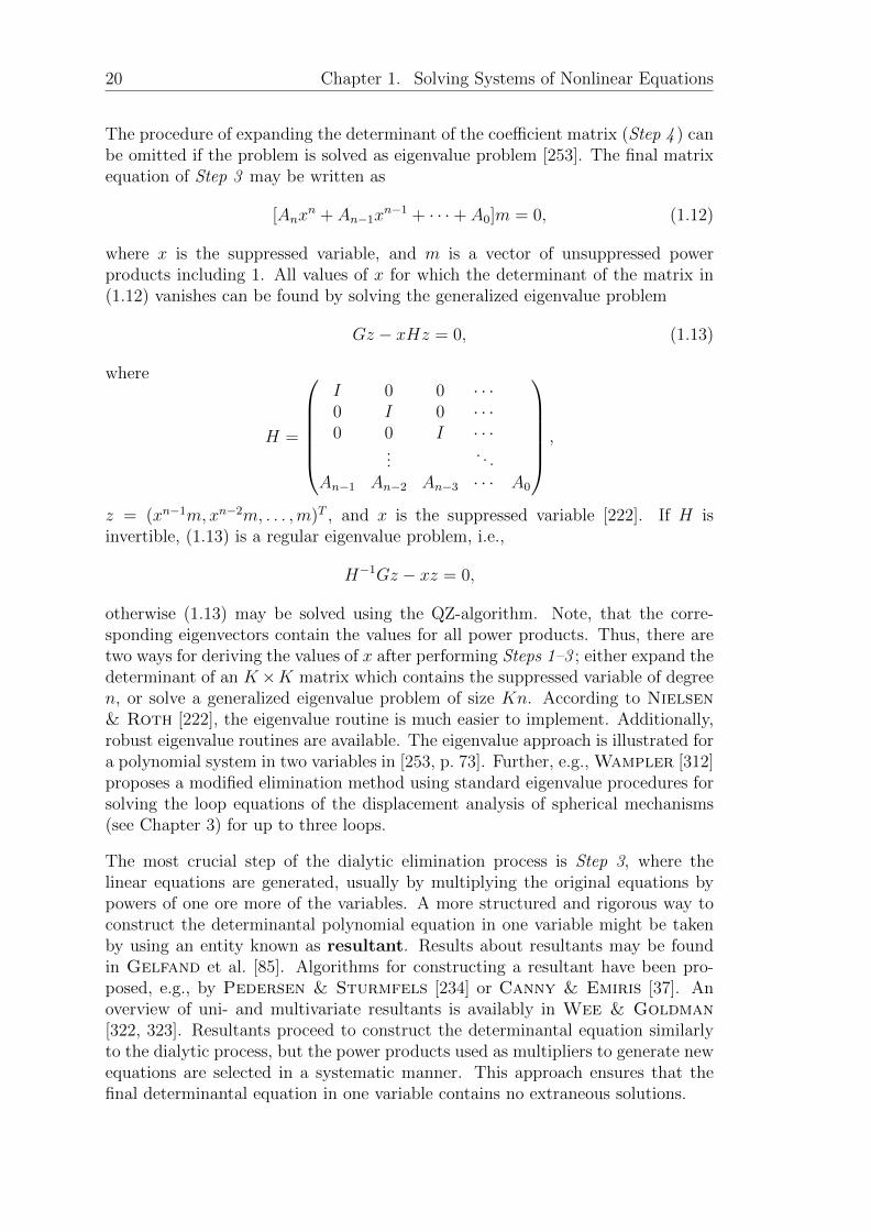
The procedure of expanding the determinant of the coefficient matrix (Step 4 ) canbe omitted if the problem is solved as eigenvalue problem [253]. The final matrixequation of Step 3 may be written as
[Anxn + An−1x
n−1 + · · ·+ A0]m = 0, (1.12)
where x is the suppressed variable, and m is a vector of unsuppressed powerproducts including 1. All values of x for which the determinant of the matrix in(1.12) vanishes can be found by solving the generalized eigenvalue problem
Gz − xHz = 0, (1.13)
where
H =
I 0 0 · · ·0 I 0 · · ·0 0 I · · ·
.... . .
An−1 An−2 An−3 · · · A0
,
z = (xn−1m,xn−2m, . . . ,m)T , and x is the suppressed variable [222]. If H isinvertible, (1.13) is a regular eigenvalue problem, i.e.,
H−1Gz − xz = 0,
otherwise (1.13) may be solved using the QZ-algorithm. Note, that the corre-sponding eigenvectors contain the values for all power products. Thus, there aretwo ways for deriving the values of x after performing Steps 1–3 ; either expand thedeterminant of an K×K matrix which contains the suppressed variable of degreen, or solve a generalized eigenvalue problem of size Kn. According to Nielsen& Roth [222], the eigenvalue routine is much easier to implement. Additionally,robust eigenvalue routines are available. The eigenvalue approach is illustrated fora polynomial system in two variables in [253, p. 73]. Further, e.g., Wampler [312]proposes a modified elimination method using standard eigenvalue procedures forsolving the loop equations of the displacement analysis of spherical mechanisms(see Chapter 3) for up to three loops.
The most crucial step of the dialytic elimination process is Step 3, where thelinear equations are generated, usually by multiplying the original equations bypowers of one ore more of the variables. A more structured and rigorous way toconstruct the determinantal polynomial equation in one variable might be takenby using an entity known as resultant. Results about resultants may be foundin Gelfand et al. [85]. Algorithms for constructing a resultant have been pro-posed, e.g., by Pedersen & Sturmfels [234] or Canny & Emiris [37]. Anoverview of uni- and multivariate resultants is availably in Wee & Goldman[322, 323]. Resultants proceed to construct the determinantal equation similarlyto the dialytic process, but the power products used as multipliers to generate newequations are selected in a systematic manner. This approach ensures that thefinal determinantal equation in one variable contains no extraneous solutions.

1.5. Elimination 21
The main disadvantage of Sylvester’s dialytic elimination method is the challengeof finding an appropriate multivariate eliminant for a particular problem. For morethan two equations there are various ways to produce the matrix A, which leadsto different polynomials with different degrees. Theoretically, Sylvester’s dialyticelimination method will reduce any system of multivariate polynomial equationsto a single polynomial in one unknown. But practically it only is applicable tosmall sets of polynomial equations, because the resulting polynomial may explodeexponentially with number and degree of equations, and may produce a largenumber of extraneous solutions [298].
The strength of elimination-based solution methods is computation time. If sucha method can be found for a particular problem, it is normally much faster thanpolynomial continuation or methods based on Grobner bases [222]. Raghavan& Roth [253] indicates that particularly dialytic procedures in combination witheigenvalue routines often produce computationally fast algorithms. Besides, theelimination method gives greater insight into a problem than purely numericalsolution methods by permitting studies of the solution space as a function of thestructural parameters of a linkage [253].
Sylvester’s dialytic elimination method is widely used in kinematics. In particular,the application to serial mechanisms is quite successful, because certain functionsof the equations are a composition of the same power products as the originalequations. Thus, the extra equations are obtained without introducing new powerproducts and so the eliminant calculation becomes feasible [222]. An example foran important application of elimination theory to kinematics is the solution of theinverse kinematics problem for serial manipulators by Raghavan & Roth [252]in 1991 (see also Chapters 3, 5). According to Raghavan & Roth [253], dialyticelimination methods are very useful for small problems with up to 6 variables,while polynomial continuation is more appropriate for large problems with manysolutions. Combinations of these methods are recommended as well, e.g., usingpolynomial continuation for determining the number of finite solutions of a largerproblem and then, if this number is not too large, constructing a solution usingdialytic elimination. More applications of the various methods are given in Chapter5.

22 Chapter 1. Solving Systems of Nonlinear Equations
Chapter 2
Interval Analysis
2.1 Introduction
The basic idea of interval analysis is to enclose numbers in intervals, and vectorsand matrices in boxes. Then, classical arithmetic and analysis are extended toor replaced by corresponding interval concepts. Intervals and ranges of functionsarise naturally in several applications. For example, measured variables (e.g., ajoint angle between two adjacent links of a robot arm) are only known approxi-mately. Hence, it is a realistic description, that the variable lies in a certain range,i.e., in an interval, whose width depends on the accuracy of the measurement.Further, in machine computations, numbers are represented with a finite numberof digits (finite precision arithmetic). This implies the presence of roundoff errorsfor the input data, the computations and, for mathematical constants. For ex-ample, with five significant digits, π ≈ 3.1416. But a sharper representation is togive the tightest representable lower and upper bounds. So, with five significantdecimal digits, π ∈ [3.1415, 3.1416] [218]. Thus, interval arithmetical tools andmethods are useful for solving problems in the presence of uncertainties in certainparameters and finite precision computer arithmetic. As uncertainties are (dueto, e.g., measurement errors) omnipresent in robotics and computations are donewith finite precision arithmetic, interval analysis methods are quite useful for thisfield of applications (see, e.g., [100, 149, 157, 195, 196, 203, 334])
Another aspect in the use of interval analysis is the certification of a derived result.For several applications in robotics for which safety is a crucial issue, e.g., medi-cal or space robotics, it is indispensable to ensure rigorous bounds on a solution(see [200, 201]). Interval algorithms provide rigorous and reliable enclosures forthe solution of numerical problems, even in the presence of round-off errors andmeasurement uncertainties.
In the following, basic properties of interval arithmetic as well as an overviewof several tools essential for solving linear and nonlinear systems of equations isgiven. The considerations are based on the book of Neumaier [218], where moredetailed explanations can be found.
23

24 Chapter 2. Interval Analysis
2.2 Basic Properties of Interval Arithmetic
2.2.1 Intervals
A (real) interval is a seta := [a, a],
with a ≤ a ∈ R := R ∪ −∞,∞, i.e., a = a ∈ R | a ≤ a ≤ a. The set of realintervals is denoted by IR and the set of nonempty bounded real intervalsby IR.
An unknown number may be represented by an approximation plus/minus an errorbound. Therefore, the midpoint a of an interval a is introduced as
a :=(a+ a)
2,
and the radius of a is given by
rad(a) :=(a− a)
2.
With these definitions the membership relation can now be expressed as
a ∈ a ⇐⇒ |a− a| ≤ rad(a),
i.e.,a = [a− rad(a), a+ rad(a)].
For the extension of the absolute value of a real number, several interval extensionsare possible. Two useful extensions are the magnitude
|a| := max|a| | a ∈ a,
and the mignitude〈a〉 := min|a| | a ∈ a
of an interval a. Usually, the terms “magnitude” and “absolute value” are usedsynonymously.
For an nonempty bounded subset S ∈ R we denote by
S := [inf (S), sup (S)]
the hull of S, i.e., the tightest interval enclosing S.
To define elementary operations, i.e., ∈ Ω := +,−, ∗, /,∧ , on the set ofintervals, let a,b ∈ IR. Then
a b := a b | a ∈ a, b ∈ b and (a, b) ∈ D[],

2.2. Basic Properties of Interval Arithmetic 25
where D[] denotes the domain of definition, in particular D[/] = IR× (IR \ 0)and D[∧] = IR+ × IR, where IR+ = a ∈ IR | a ≥ 0.
The extension of elementary functions ϕ : R→ R to ϕ : IR→ IR is defined as
ϕ(a) := ϕ(a) | a ∈ a, a ∈ D(ϕ).
We will only use this form of extending univariate functions for a fixed set Φ ofelementary functions
Φ = log, exp, sin, cos, sinh, cosh, •n(n ∈ N), n√•(n ∈ N), arctan, abs.
In most cases, the lower and upper bounds of the resulting intervals can be com-puted by using the endpoints of the given intervals. For example, the addition oftwo intervals is given by a + b = [a + b, a + b]. For multiplication and division,the result depends on the signs of a and b, and for division the result additionallydepends on whether 0 ∈ a and/or 0 ∈ b. A detailed description is given in [218,Ch. 1.2].
2.2.2 Rounded interval arithmetic
When interval arithmetic is realized on a computer, intervals in general haveto be rounded. This is because there is only a finite set M ∈ R of machine-representable numbers (in most cases the floating point numbers). Therefore,the optimal directed rounding operations are defined as
∇r := supxm ∈M | xm ≤ r, ∇ : R→M, and
∆r := infxm ∈M | xm ≥ r, ∆: R→M
for rounding downwards and for rounding upwards, respectively. With thisnotations, the optimal outward rounding is given by
: IR→ IM[a, a] 7→ [∇a,∆a],
where IM denotes the subset of IR such that a ∈ IM if and only if a, a ∈ M. So,all arithmetic operations ∈ Ω and elementary functions ϕ ∈ Φ on a computerare defined by
a b := (a b),
ϕ(a) := ϕ(a).
Note, that it implicitly is assumed that ±∞ ∈M, 0 ∈M and so, rounding upwardsand downwards, respectively, always exists.

26 Chapter 2. Interval Analysis
2.2.3 Boxes, interval vectors, and interval matrices
To cover expressions in several variables, some notation for interval vectors andinterval matrices is introduced. Let IRn be the space of interval vectors, i.e.,the space of column vectors of intervals, also called boxes. Then x ∈ IRn is givenby
x = [x, x] = x ∈ Rn | x ≤ x ≤ x
with x, x ∈ Rn. In a similar way, interval matrices are defined. An m× n interval
matrix is a rectangular array of intervals Aik ∈ IR. Let IRm×nbe the set of all
m× n interval matrices, then
A = [A,A] = A ∈ Rm×n | A ≤ A ≤ A
with A,A ∈ Rm×n. If Σ is a bounded set of real m × n matrices, then its hull is
defined asΣ := [inf(Σ), sup(Σ)],
which is the tightest interval matrix enclosing Σ.
An important abstract tool for the study of iterative methods for the solution oflinear and nonlinear systems of equations is the notion of sublinear mappings,which are mappings S : IRn → IRn which satisfy the axioms
(S1) x ⊆ y =⇒ Sx ⊆ Sy (inclusion isotonicity),
(S2) α ∈ R =⇒ S(αx) = α(Sx) (homogeneity), and
(S3) S(x + y) ⊆ Sx + Sy (subadditivity)
for all x,y ∈ IRn. If equality holds in (S3), the mapping is called linear. Twoimportant tools for analyzing sublinear mappings are the absolute value of S,defined as
|S| := |S[−1,1]|,
and the core of S, given by
cor(S) := S1 = (Se1, . . . , Se2).
Theorem 2.2.1. Let S : IRn → IRm be sublinear. Then
| cor(S)| ≤ |S|,Sx ⊆ cor(S)x+ |S|(x− x) ∀x ∈ IRn. (2.1)
If S is linear, then equality holds in (2.1). In particular, a linear mapping isuniquely determined by its core and its absolute value.
Proof. See Neumaier [218, Thm. 3.5.4].
2.2. Basic Properties of Interval Arithmetic 27
A linear interval equationAx = b
with coefficient matrix A ∈ IRm×n and right-hand side b ∈ IRm is defined as thefamily of linear equations
Ax = b with A ∈ A, b ∈ b. (2.2)
We are interested in enclosing its solution set, given by
Σ(A,b) := x ∈ Rn | Ax = b for some A ∈ A, b ∈ b. (2.3)
In general, Σ(A,b) is not an interval vector and may have a very complicatedstructure. In order to guarantee its boundedness, A is required to be regular,i.e., that rank(A) = n for all A ∈ A. Thus, if A ∈ IRn×n the hull of the solutionset
AHb := Σ(A,b)
is defined and, in particular, defines a mapping AH : IRn → IRn, the so-calledhull inverse of A. For rectangular matrices A ∈ IRm×n (and m ≥ n, becauseotherwise Σ(A,b) is either empty or unbounded and thus, AHb is not defined),it makes sense to consider instead of (2.3) the least squares solution set
ΣLS(A,b) := A†b | A ∈ A, b ∈ b,
where A† = (AT A)−1AT is the pseudo-inverse of A, and the least squares hullof A and b, given by
ALb := ΣLS(A,b).
Clearly,AHb ⊆ ALb.
The solution set Σ(A,b) of (2.2) has the following neat characterization
Theorem 2.2.2 (Beeck). Let A ∈ IRm×n,b ∈ IRm. Then
Σ(A,b) = x ∈ Rn | Ax ∩ b 6= 0 = x ∈ Rn | 0 ∈ Ax− b.
Proof. See Neumaier [218, Thm. 3.4.3].
The matrix inverse of a regular, square interval matrix A ∈ IRn×n can be definedas
A−1 := A−1 | A ∈ A.
An inverse positive matrix is a regular square interval matrix with nonnegativeinverse. The most important subclass of these consists of so-called M -matrices,which play a distinguished role in the context of interval calculations, as theybehave particularly well in algorithms for the solution of linear interval equations.An M -matrix is a square matrix A ∈ IRn×n such that Aik ≤ 0 for all i 6= k, andAu > 0 for some positive vector u ∈ Rn. Every M -matrix is regular. Furthermore,
28 Chapter 2. Interval Analysis
for inverse positive matrices the inverse A−1 and the hull inverse AHb can becomputed explicitly (see [218, Ch. 3.6]).
A generalization of M -matrices, the so-called H -matrices, are obtained by liftingthe restrictive sign condition in the definition of an M -matrix. Therefore, thecomparison matrix 〈A〉 with entries
〈A〉ik :=
〈Aik〉 if i = k
−|Aik| if i 6= k
is introduced for an arbitrary square matrix A ∈ IRn×n. The comparison matrixalways fullfills the sign-condition of an M -matrix. Now, an H -matrix is a squarematrix A ∈ IRn×n such that its comparison matrix 〈A〉 is an M -matrix; equiva-lently, A is an H -matrix if and only if 〈A〉u > 0 for some u > 0. In particular,every H -matrix is regular and 0 /∈ Aii for all i = 1, . . . , n.
Every M -matrix is an H -matrix. In the special case u = (1, . . . , 1)T , a matrixA satisfying 〈A〉u > 0 is called a strictly diagonally dominant matrix. It isan important fact, that a matrix which is sufficiently close to the identity matrix,is strictly diagonally dominant, and therefore an H -matrix. For example, everyregular (lower or upper) triangular matrix A ∈ IRn×n is an H -matrix.
2.2.4 Interval extensions of arithmetic expressions
If D ⊆ Rn, then ID is written for the set of intervals x ∈ IRn
with x ⊆ D. Aninterval function f : ID ⊆ IRn → IRm
is called inclusion isotone if,
a ⊆ b =⇒ f(a) ⊆ f(b) ∀a,b ∈ ID.
Further, an interval function f : IRn → IRmis said to be an interval extension
of the real function f0 : D ⊆ Rn → Rm if
f(x) = f0(x) ∀x ∈ D, (2.4a)
f0(x) ∈ f(x) ∀x ∈ x ∈ ID, (2.4b)
f(x) = NaN for x /∈ ID, (2.4c)
where the symbol NaN stands for “not a number”, which may be thought of as“undefined” or “unspecific value”. If only (2.4b) and (2.4c) are satisfied, f is calleda weak interval extension or an interval enclosure of f0. A large class of in-clusion isotone interval extensions of real functions can be defined through arith-metic expressions. An arithmetic expression in the formal variables ξ1, . . . , ξnis a member of the set A = A(ξ1, . . . , ξn) defined by
(i) R ∈ A,
(ii) ξl ∈ A for l = 1, . . . , n,

2.2. Basic Properties of Interval Arithmetic 29
(iii) g, h ∈ A =⇒ (g h) ∈ A for all ∈ Ω,
(iv) g ∈ A =⇒ ϕ(g) ∈ A for all elementary functions ϕ ∈ Φ,
(v) among the sets which satisfy (i)–(iv), A is minimal with respect to inclusion.
A subexpression of an arithmetic expression f is an expression occurring in therecursive definition of f , formally, k is a subexpression of f if either
(i) f = k, or
(ii) f = g h and k is a subexpression of g or h, or
(iii) f = ϕ(g) and k is a subexpression of g.
If f = f(ξ) is an arithmetic expression in n variables, the value f(x) of f atx ∈ IRn is obtained by substituting the intervals xi for the corresponding formalparameters ξi (interval evaluation). On a computer the interval evaluation issimulated by a rounded evaluation, the outward rounded value of f is denotedby f (x).
2.2.5 Enclosures for the range of a function
Useful general results about the interval evaluation of arithmetic functions can beobtained, if the evaluation at intervals are avoided, in which the expressions arenot sufficiently smooth. Therefore, Lipschitz properties for interval functions andarithmetic expressions are introduced.
An interval function f : IRn → IR is called Lipschitz continuous in x0 ∈ IRn,if x0 ⊆ D and there exists l0 ∈ Rn such that
q(f(x1), f(x2)) ≤ l0 q(x1,x2) ∀ x1,x2 ⊆ x0,
where q(a,b) := |a− b|+ | rad(a)− rad(b)| is the distance function, which is usedcomponent-wise on vectors. An arithmetic expression f in n variables is calledLipschitz at x0 ∈ IRn if for all subexpressions g, h of f , the relation g = hα
for 0 < α < 1 implies h(x0) > 0, and the relation g = ϕ(h) for ϕ ∈ Φ impliesthat ϕ is defined and Lipschitz continuous in a neighborhood of h(x0). f is calledlocally Lipschitz in x0 ∈ IRn if f is Lipschitz at every x ∈ x0. For the standardelementary functions the property of being Lipschitz only is marginally strongerthan the property of being defined.

30 Chapter 2. Interval Analysis
The mean value form and other centered forms
The interval evaluation f(x) of an arithmetic expression f in n variables at aninterval x ∈ IRn is an enclosure for the range
f ∗(x) := f(x) | x ∈ x.
However, the overestimation may be large. Therefore, methods are needed toenclose the range f ∗(x) in such a way that the overestimation remains small forsufficiently narrow boxes x. A very useful approach to bound the range is toconsider the deviation of f(x) from a fixed center z ∈ x. Thus, the resultingformulae are called centered forms. The simplest one is the mean value form
fm(x) := f(x) + f ′(x)(x− x). (2.5)
Note that different expressions for the derivative f ′ may change the value of (2.5)(sometimes quite drastically), while different expressions f for the same real func-tion do not affect the value of (2.5). The mean value form can be shown to beinclusion isotone. Further, it satisfies the important quadratic approximationproperty
0 ≤ rad(fm(x))− rad(f ∗(x)) ≤ 2 rad(f ′(x)) rad(x),
which expresses the overestimation of the range by a product of two radii. Inparticular, for narrow intervals the mean value form in general gives a much betterenclosure for the range than the interval evaluation.
To derive more general centered forms, the notion of slopes shall be introduced.For a Lipschitz continuous function f : Rn → R one can always write
f(x) = f(z) + f [z, x](x− z)
for any two points x and z with a suitable vector f [z, x] ∈ Rn, called a slopevector for f at (z, x). In the univariate case (n = 1)
f [z, x] =
f(x)−f(z)
x−z if x 6= z,
f ′(z) if x = z,
hence f [z, x] is uniquely determined. In the multivariate case, however, the slopef [z, x] is no longer unique while f [z, z] = ∇f(z), i.e., the gradient of f. As slopesobey a similar chain rule as derivatives, recursive procedures to calculate f [z, x]given x and z can be developed (see, e.g., Krawczyk & Neumaier [150]). If wehave a slope f [z, x] for all x ∈ x and f [ζ, ξ] is an arithmetic expression in ζ and ξ,then the range f ∗(x) can also be enclosed by the slope form with center z ∈ x,defined as
fs,z(x) := f(z) + f [z,x](x− z). (2.6)
The slope form is inclusion isotone as well. More generally, formulae f(z)+sT (x−z)(s ∈ IRn), for which f(x) = f(z) + sT (x− z) holds for all x ∈ x and some s ∈ s,
2.3. Solving Linear Systems of Equations 31
are called centered form for f with center z. All centered forms satisfy theoverestimation bound
q(f(z) + sT (x− z), f ∗(x)) ≤ 2 rad(s)|x− z|,
but need not to be inclusion isotone. However, for fixed centers inclusion isotonic-ity is a trivial consequence of (2.6).
A further improvement for the enclosure for the range is obtained by taking twodifferent centers z and w intersecting the two corresponding slope forms and getso-called bicentered forms
fb(x) := fs,z(x) ∩ fs,w(x).
If the slope vector f [z, x] itself is Lipschitz continuous, it can be written as
f [z, x] = f [z, w] + (x− w)Tf [w, z, x] (2.7)
for arbitrary x,w, z ∈ Rn, with a second order (bicentered) slope matrixf [w, z, x] ∈ Rn×n [273]. Using this the second order slope for f at z and w, a rangeestimate for f can be computed using the second order slope form, given by
fss,z,w(x) := f(z) + (f [z, w] + (x− w)Tf [w, z,x])(x− z).
These estimates in general are tighter than analogous ones computed by intervalderivatives. All second order centered forms have a cubic approximation property.Slopes of arbitrary order can be derived by defining a slope of order k in the sameway as in (2.7) as a slope of slopes of order k − 1 [273].
2.3 Solving Linear Systems of Equations
For solving linear systems of equations, the class of strongly regular matrices (seebelow) is an important feature. It can be shown, that for linear interval equationswith a strongly regular coefficient matrix the solution set can be enclosed by thesolution set of a related, preconditioned system whose coefficient matrix is anH -matrix. If x is a solution of the system
Ax = b for A ∈ A regular, b ∈ b, (2.8)
and rad(A) is sufficiently small, then A ≈ A, and x = A−1b ≈ A−1b. The errormade can be analyzed by multiplying (2.8) by A−1.Thus, x is the solution of asystem with coefficient matrix A−1A ≈ 1 and right-hand side A−1b. Hence,
x ∈ Σ(A−1A, A−1b) ⊆ (A−1A)H(A−1b)
if A−1A is regular. The transformation above is called preconditioning by themidpoint inverse, and A−1 is called the preconditioner or midpoint precon-ditioner. A matrix A ∈ IRn×n is called strongly regular if A−1A is regular.

32 Chapter 2. Interval Analysis
In particular, A being strongly regular is equivalent to A−1A being an H -matrix.However, a useful preconditioning does not depend on A−1 as preconditioner. In-stead, A can be multiplied by any matrix C ∈ Rn×n and further, it can also bepost-multiplied by some matrix C ′ ∈ Rn×n, as long as the resulting matrix isregular.
In the following, two methods for solving linear interval systems of equations areoutlined, namely Krawczyk iteration and interval Gauss-Seidel iteration.
Krawczyk iteration
Krawczyk’s iteration method provides computable bounds for the overestimationof an enclosure of AHb as well as enclosures which have the quadratic approxima-tion property. It can be shown that for a square system of linear equations witha strongly regular coefficient matrix, a (rather crude) enclosure for the hull AHbof the solution set is given by
AHb ⊆ ‖Cb‖v[−u, u], (2.9)
if u > 0, and 〈CA〉u ≥ v > 0. A better enclosure might be derived from (2.9),if an approximation x to a particular solution is found first and then added toan enclosure for the residual correction AH(b − Ax) (obtained using (2.9). Inparticular, AHb ⊆ x+ AH(b−Ax). If b−Ax is of order O(ε), this causes that
AHb ⊆ x+ ‖C(b−Ax)‖v[−u, u] (2.10)
has an overestimation of O(ε) and thus, it is an enclosure for AHb with linearapproximation order. A method with quadratic approximation order can be real-ized by improving the initial enclosure (2.10) iteratively. Therefore, consider therelation
A−1b = Cb− (CA− 1)(A−1b) ∈ Cb− (CA− 1)x,
where x is an enclosure for AHb. This holds for all A ∈ A and b ∈ b, implying
AHb ⊆ x =⇒ AHb ⊆ (Cb− (CA− 1)x) ∩ x.
This relation is the input to the so-called Krawczyk iteration
z0 := x
zl+1 := (Cb− (CA− 1)zl) ∩ zl.
The zl form a nested sequence of interval vectors, and by construction AHb ⊆ ximplies AHb ⊆ zl for all l ≥ 0. It can be shown (see [218, Ch. 4.2]), that forinterval input whose radii are small enough the Krawczyk iteration has quadraticapproximation order, i.e., if the enclosure (2.10) is used as an initial enclosure forthe iteration the Krawczyk iterates zl with l ≥ 1 enclose the hull AHb of thesolution set Σ(A,b) with quadratic approximation order. For CA close to theidentity, in the limit the Krawczyk iteration produces enclosures of AHb whichhave a bounded radius overestimation factor independent of the right-hand side.Therefore, after sufficiently many iterations, reliable enclosures are also obtainedfor wide right-hand sides b (see [218, Thm. 4.2.4]).
2.3. Solving Linear Systems of Equations 33
Interval Gauss-Seidel iteration
Krawczyk’s iteration is a reliable method for deriving realistic enclosures of thesolution set of linear equations whose coefficients are narrow intervals. However,there is a superior method, the so-called interval Gauss-Seidel iteration. For M -matrices A, Gauss-Seidel iteration converges for every b ∈ IRn to the hull AHbof the solution set (see [218, Thm. 4.4.8]). If Gauss-Seidel iteration is applied to apreconditioned system, it always yields at least at tight intervals as the Krawczykiteration (see [218, Thm. 4.3.5]).
For arbitrary x ∈ IRn, good enclosures for the truncated solution set
Σx(A,b) := Σ(A,b) ∩ x = x ∈ x | Ax = b for some A ∈ A, b ∈ b
shall be found. Note, that Σx is bounded, even if A is singular. Gauss-Seideliteration is based on writing the system Ax = b explicitly in components as
n∑k=1
Aikxk = bi (i = 1, . . . , n),
and, assuming that Aii 6= 0, the ith equation is solved for the ith variable. Hence,
xi =1
Aii(bi −
∑k 6=i
Aikxk) ⊆1
Aii
(bi −∑k 6=i
Aikxk) ∩ xi =: x′i. (2.11)
If Aii 6= 0 for all i, relation (2.11) can be applied for all i and thereby, a newenclosure x′ for x can be computed from a known interval vector x containingx. However, the available information can be used in an improved way. In theith step, an enclosure for xi and improved enclosures for xi, . . . , xi−1 are alreadyavailable and can be used to obtain an improved enclosure of the right-hand sideof (2.11) to get an improved enclosure for xi. Thus, x is contained in the vector ygiven by
yi :=1
Aii
(bi −∑k<i
Aikyk −∑k>i
Aikxk) ∩ xi (i = 1, . . . , n).
For intervals a,b,x ∈ IR we define
Γ(a,b,x) := x ∈ x | ax = b for some a ∈ a, b ∈ b.
Then
Γ(a,b,x) =
b/a ∩ x if 0 /∈ a,
(x\ ] ba, ba[) if b > 0 ∈ a,
(x\ ] ba, ba[) if b < 0 ∈ a,
x otherwise.
In extension of the notation we define the (interval) Gauss-Seidel operatorΓ(A,b,x) with entries
Γ(A,b,x)i := Γ(Aii,bi −∑k<i
Aikyk −∑k>i
Aikxk,xi) (i = 1, . . . , n).

34 Chapter 2. Interval Analysis
If Γ(A,b,x) $ x, we can hope to further improve the enclosure of AHb by reap-plying Γ. Thus, the interval Gauss-Seidel iteration is defined by
x0 := x
xl+1 := Γ(A,b,xl) for l = 0, 1, 2, . . . ,
and the preconditioned Gauss-Seidel iteration for C ∈ Rn×n can be definedsimilarly with xl+1 := Γ(CA, Cb,xl). We then have Σx(A,b) ⊆ Σx(CA, Cb) ⊆ xl
for all l ≥ 0.
2.4 Solving Nonlinear Systems of Equations
Now we consider the problem to determine whether a continuous function F : D0 ⊆Rn → Rn has a zero x∗ in a given subset D ⊆ D0 and when such a zero is unique.Therefore, the Newton operator, the Krawczyk operator and the Hansen-Senguptaoperator are introduced, which provide simple computational tests for (unique)existence and nonexistence of a zero in a given box. To obtain uniqueness results,a form of Lipschitz continuity is assumed, while the existence problem can betreated assuming only that F is continuous.
A subset A ⊆ Rm×n is called a Lipschitz set for F on D ⊆ D0 if it is convex,compact, and
F (x)− F (y) = A(x− y) for some A ∈ A
holds for every x, y ∈ D. If additionally A ∈ IRm×n, it is called a Lipschitzmatrix. In particular, for every interval extension of the derivative F ′ on D thematrix A = F ′(x) is a Lipschitz-matrix, if F is continuously differentiable in D,x ∈ ID and A ∈ IRm×n. A Lipschitz set A of matrices A ∈ Rn×n is called regularif all A ∈ A are nonsingular.
Theorem 2.4.1 (Moore, Nickel). Let F : D0 ⊆ Rn → Rn be Lipschitz continuouson D ⊆ D0, and let A be a regular Lipschitz matrix on D. If x ∈ x ∈ ID thenevery x′ ∈ IRn satisfying
N(x, x) := x−AHF (x) ⊆ x′
has the following three properties:
(i) Every zero x∗ ∈ x of F satisfies x∗ ∈ x′.
(ii) If x′ ∩ x = ∅ then F has no zeros in x.
(iii) If x ∈ int(x) and x′ ⊆ x then F contains a unique zero in x (and hence inx′).
Proof. See Neumaier [218, Thm. 5.1.7].
2.4. Solving Nonlinear Systems of Equations 35
Note, that the condition x ∈ int(x) in (iii) can be replaced by the more practicalrequirement x′ ⊆ int(x). N(x, x) is called the (interval) Newton operator andcan be interpreted as a verified version of the Newton iterate, which yields enclo-sures for the zero of F (which is unique under the present assumptions). Further-more, N(x, x) provides a nonexistence test (Theorem 2.4.1(ii)) and an existenceand uniqueness test (Theorem 2.4.1 (iii)), which are not available in the classicalNewton iteration. However, the Newton operator requires A to be regular.
There are two more operators, which basically have the same properties as theNewton operator, but can be defined for a Lipschitz-matrix A and thus are morewidely applicable. These are the Krawczyk operator, which is given by
K(x, x) := x− CF (x)− (CA− 1)(x− x),
and the Hansen-Sengupta operator, which is defined as
H(x, x) := x+ Γ(CA,−CF (x, (x− x)).
Those are nonlinear variants of the Krawczyk iteration and the interval Gauss-Seidel iteration. Note, that both operators involve a preconditioning matrix C.The inclusion
H(x, x) ⊆ K(x, x) (2.12)
holds for all x ∈ x ⊆ x0. Hence, the Hansen-Sengupta operator gives at least asgood enclosures for a zero of F as the formally simpler Krawczyk operator. Aresult similar to Thm. 2.4.1 holds with H(x, x) and K(x, x), but with a weakerexistence test than with N(x, x).
Let P(x, x) be any of N(x, x), K(x, x) and H(x, x). Then an iteration for improvinginterval enclosures of a zero x∗ of a function F by repeated application of P(x, x)is defined as
x0 := x
xl+1 := P (xl, xl) ∩ xl (l ≥ 0, xl ∈ xl). (2.13)
By construction,xl+1 ⊆ xl ⊆ · · · ⊆ x0 = x, (2.14)
and we knowx∗ ∈ x with F (x∗) = 0 =⇒ x∗ ∈ xl ∀l ≥ 0. (2.15)
In particular, the limitx∞ := lim
l→∞xl
exists, and if the starting box x contains a zero x∗ of F then x∗ ∈ x∞. Note that infinite precision arithmetic the expression F (x) in the operator P(x, x) needs to beevaluated with outward rounding. Otherwise the solution may suddenly disappear(xl+1 = ∅) due to rounding errors. Under suitable conditions it can be shown thatthe following alternative holds:

36 Chapter 2. Interval Analysis
(SC) Either F has a unique zero x∗ ∈ x and x∞ = x∗,or F has no zero in x and xl = ∅ for some l ≥ 0.
In particular, if (SC) holds, the iteration is capable of deciding whether thereis a zero of F in x or not, and, assuming sufficiently accurate arithmetic, thezero can be enclosed with arbitrary accuracy. A sequence xl (l = 0, 1, 2, . . . )satisfying (2.14) and (2.15) is called strongly convergent, if (SC) holds. Forthe Krawczyk iteration (P(x, x) = K(x, x) in (2.13)) strong convergence can beproven for the choice xl = xl and, under strengthened assumptions, for otherchoices of x as well. Since (2.12) always holds, these results immediately extendto the Hansen-Sengupta iteration (P(x, x) = H(x, x) in (2.13)). In that case, muchweaker assumptions are sufficient to prove strong convergence. However, resultsabout convergence rates have not been obtained under these weaker conditions.
In order to consider convergence conditions for the Newton-iteration, we con-sider the general preconditioned Newton-iteration, i.e., P(x, x) = NI(x, x)in (2.13) with the general Newton operator
NI(x, x) := x− (CA)I(CF (x)),
where C ∈ Rn×n is a preconditioning matrix and (CA)I denotes an inverse of(CA), i.e., a sublinear mapping with (CA)Hb ⊆ (CA)Ib for all b ∈ IRn. If(CA)I is regular, the general Newton iteration is strongly convergent for everychoice xl ∈ xl. Moreover, for all l ≥ 0,
either xl /∈ xl+1, or xl+1 = xl and F (xl) = 0. (2.16)
Relation (2.16) implies a volume-reducing property of the Newton iteration. Morespecifically, the general Newton iteration with xl = xl satisfies
vol xl+1 ≤ 12
vol xl, (2.17)
where vol x := (x1 − x1)(x2 − x2) · . . . · (xn − xn) denotes the volume of a boxx ∈ IRn. Further, if CA is an M -matrix or ‖1 − CA‖ < 1
2, then the optimal
Newton iteration, i.e., the general Newton iteration (P(x, x) = NI(x, x))withC = 1 and AI = AH , is strongly convergent for every choice of xl ∈ xl, and (2.16)and (2.17) hold.
Summarizing the results, Hansen-Sengupta iteration strongly converges under themildest assumptions, but it may have a slow convergence rate, and not even agood approximation to the zero can accelerate the iteration. Newton iteration, onthe other hand, considerably speeds up using good approximations to the zero.However, when the hull inverse is replaced by an easier computable inverse, theiteration may stop prematurely. But a combination of both methods, given by
x0 := x
xl+1/2 := NI(x, xl) ∩ xl
xl+1 := H(xl+1/2, xl),

2.4. Solving Nonlinear Systems of Equations 37
where xl ∈ xl for all l ≥ 0, CA is an H -matrix, and (CA)I is an inverse of CA,preserves the advantages and avoids the disadvantages of both methods. With thiscombination an algorithm can be produced, which decides whether a zero x∗ of Fis contained in a given box x ∈ IRn and if affirmative, finds a good enclosure ofx∗. The relation xl+1 ⊆ xl and finite precision arithmetic imply finite terminationof the iteration.
For finding zeros of continuous parameter-dependent functions which are not nec-essarily Lipschitz continuous, general existence results can be derived. However,due to the weaker assumptions, uniqueness results can no longer be proved. In asimilar way as the centered forms are sharpened when slopes are used instead ofderivatives, the use of slopes in place of Lipschitz sets improves the enclosure anditeration methods for deriving zeros (for details see Neumaier [218, Ch. 5.4].)
Finally, we have discuss methods for computing narrow enclosures for all solutionsx∗ ∈ D of F (x∗) = 0 with F : D0 ⊆ Rn → Rn continuous. The methods consideredso far were constructive only in the case when D was a box and the Lipschitz matrixof F at this box was regular. If these assumptions are dropped, on the one hand,the problem has to be reduced to one with bounded domain. This can be handledusing a priori bounds or suitable problem transformations. On the other hand,the existence of several solutions may be possible. Therefore bisection is used.Assume that zeros are sought in a box x0 ∈ IRn. If this box is narrow enough,one of the above described methods can be applied. In the case that x0 is toowide, bisection methods must replenish the former methods. The basic principleof bisection is to split boxes repeatedly, until they can be further reduced bymeans of interval iteration. Therefore, a list of currently unprocessed boxes arestored in a so-called stack or queue. If there are several isolated solutions in theinitial box x0, they will be isolated by bisection.
Interval analysis based algorithms are frequently used in global optimization,where the absolute minimum of the objective function F is sought. Therefore,branch & bound-algorithms are used (see, e.g., Moore et al. [208]). How-ever, these methods frequently have the difficulty that subboxes containing nosolution cannot be eliminated easily if they are close to the global minimum.Thus, the so-called cluster effect occurs. That means, many small boxes arecreated near each global minimum (and, in the process of solving the problem alsonear the currently best found local minimum) by repeated splitting, and often theprocessing of these boxes dominates the total work spent on the global search.The cluster effect can be reduced by defining exclusion regions around each localminimum found. It is guaranteed, that exclusion regions do not contain other lo-cal minima, and can therefore safely be discarded. Recently, Schichl et al. [274]discussed exclusion regions, which are constructed using uniqueness tests based onthe Krawczyk operator.

38 Chapter 2. Interval Analysis

Part II
Robotics
39

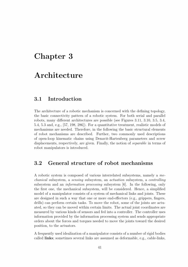
Chapter 3
Architecture
3.1 Introduction
The architecture of a robotic mechanism is concerned with the defining topology,the basic connectivity pattern of a robotic system. For both serial and parallelrobots, many different architectures are possible (see Figures 3.11, 3.10, 3.5, 3.4,5.4, 5.3 and, e.g., [57, 198, 286]). For a quantitative treatment, realistic models ofmechanisms are needed. Therefore, in the following the basic structural elementsof robot mechanisms are described. Further, two commonly used descriptionsof open-loop kinematic chains using Denavit-Hartenberg parameters and screwdisplacements, respectively, are given. Finally, the notion of separable in terms ofrobot manipulators is introduced.
3.2 General structure of robot mechanisms
A robotic system is composed of various interrelated subsystems, namely a me-chanical subsystem, a sensing subsystem, an actuation subsystem, a controllingsubsystem and an information processing subsystem [6]. In the following, onlythe first one, the mechanical subsystem, will be considered. Hence, a simplifiedmodel of a manipulator consists of a system of mechanical links and joints. Theseare designed in such a way that one or more end-effectors (e.g., grippers, fingers,drills) can perform certain tasks. To move the robot, some of the joints are actu-ated, so they can be moved within certain limits. The actual joint coordinates aremeasured by various kinds of sensors and fed into a controller. The controller usesinformation provided by the information processing system and sends appropriateorders about the forces and torques needed to move the joints toward the desiredposition, to the actuators.
A frequently used idealization of a manipulator consists of a number of rigid bodiescalled links; sometimes several links are assumed as deformable, e.g., cable-links,
41

42 Chapter 3. Architecture
which complicate the analysis of the manipulator. In the following, only mecha-nisms with rigid links are considered. Usually, a manipulator is fixed to an initiallink, the base; the final link is called the end-effector. Links are coupled byjoints to so-called kinematic pairs. There are two basic types of joints (seeFigure 3.1):
Prismatic pairs (P) are links joined by a sliding prism with a definite direction.The motions possible are extension and retraction.
Revolute joints (R) are links connected by a joint with a definite rotation axis.
Figure 3.1. Symbolic representation ofrevolute and prismatic joints [286, p. 13].
The following joint types are commonly used as well. However, these types can bereplaced by a concatenation of prismatic or revolute pairs.
Spherical joints (or ball-and-socket joints) are joints where three rotationalaxes intersect. They are equivalent to three revolute joints (RRR) whoseaxes have a common center.
Universal joints are equivalent to two revolute joints (RR) whose axes intersect.
Cylindrical joints are equivalent to one revolute and one prismatic pair with acommon axis.
Kinematic types can also be distinguished by the type of contact between the twolinks. Two rigid bodies form an upper kinematic pair, when contact takes placealong a line or at a point, e.g., in cam-and-follower mechanisms or gear trains [6].In a lower kinematic pair contact takes place along a common surface betweenthe two bodies. According to Angeles [6], six different forms of lower kinematicpairs can be distinguished (see Fig. 3.2).
If a kinematic pair can be moved by a motor (actuator), it is called actuatedjoint. An actuated kinematic pair is called a linear (P) or rotary (R) actuator.Pairs which are not actuated adjust themselves to forces imposed by loads andactuators, i.e., these pairs perform only passive motion and therefore are calledpassive. The motion of actuated joints is restricted by certain limits accordingto the actual construction of the robot.

3.2. General structure of robot mechanisms 43
Figure 3.2. The six lowerkinematic pairs [57, p. 63].
A rigid body in space can move in various ways by rotation or translation. Theseare called degrees of freedom (d.o.f.). The total number of d.o.f. of a rigidbody in 3-dimensional space is at most six (see Fig. 3.3). Each revolute andprismatic joint, respectively, in a kinematic chain is a 1-d.o.f. joint. In the formercase the degree of freedom is given by the angle of rotation, in the latter case bythe amount of linear displacement. Hence, the total number of degrees of freedomof a robot is the number of independent position variables needed to specify thespatial pose (i.e., position and orientation) of the end-effector (see also Chapter 4).For many applications, less than 6 d.o.f. are needed. Thus, the number of d.o.f.should match the number required by the desired task, at least for serial robots[57]. For parallel robots, Merlet [198, p. 19f] takes a critical point of view ofthe usual claim, that machines having only the necessary d.o.f. will be less costlythan the usual 6 d.o.f. parallel manipulator. He states that various factors mayincrease the operating cost of a less than 6 d.o.f. robot, e.g., higher maintenanceand fabrication cost because of different actuators/sensors involved in the chains,or exhibition of parasitic motion (i.e., motion that is not wanted) which affectsthe robots performance.
To view joints from an algebraic point of view, we need the special Euclideangroup
SE(3) = (c,Q) | c ∈ R3, Q ∈ SO(3) = R3 × SO(3),
withSO(3) = Q ∈ R3×3 | QTQ = QQT = 1, detQ = 1
denoting the special orthogonal group, i.e., the group of rotations in R3. Then,joints are surfaces of contact between links that constrain the motion of the robotmechanism to a subset of SE(3)n−1: without the joints, each link could move with6 d.o.f. anywhere in SE(3). Typically, the locations of the links are measuredrelatively to the base; thus, a concatenation of n links ‘lives’ in SE(3)n−1. Ajoint which constrains a mechanism to an algebraic subset of SE(3)n−1 is calledalgebraic joint. Five of the six lower-order pairs in Figure 3.2 are algebraic.The only exception is the screw (or helical) joint, whose transformation matrix

44 Chapter 3. Architecture
consists of an angle α as well as sinα and cosα, which make the motion trulytrigonometric, hence non-algebraic [313].
Figure 3.3. 6 degrees of freedom: 3 componentsof translation, 3 components of rotation[www.dovermotion.com].
An open kinematic chain is a chain of links, where each but the first andthe last link is coupled to exactly two other links. For a quantitative treatment,it is helpful to characterize open- and closed-loop kinematic chains, respectively,by the degree of connectivity (or connection degree) of each link [88]. Itis defined as the number of rigid bodies directly attached to a certain link bykinematic pairs. Therefore, in a simple kinematic chain each member possessa connection degree of at most 2. An open kinematic chain is defined as a simplekinematic chain, where exactly two links (the base and the end-effector) haveconnectivity 1. A closed-loop kinematic chain is obtained when the connectiondegree of one of the links (not the base) is at least 3 [198].
Figure 3.4. A serial manipulator with 6 d.o.f. (T3) [152].
A robot consisting of a single open kinematic chain is called a serial robot orserial manipulator. It is best visualized as a movable mechanical arm. A robotwhose only end-effector (the platform) with n d.o.f. is connected to a fixed baseby at least two independent open kinematic chains (the legs) is called parallel

3.3. Description of open-loop kinematic chains 45
robot or parallel manipulator [198]. It is actuated by n simple actuators. Amanipulator containing at least one closed-loop kinematic chain is called hybrid;see, e.g., [50, 292]. An important class of parallel architectures is the one of fullyparallel robots, where the number of kinematic chains is strictly equal to thenumber of d.o.f. of the platform [88]. For example, a 6 d.o.f. fully parallel robotconsists of arbitrarily shaped base and platform connected by six legs. Each legcontains six kinematic pairs, of which one is linearly or rotary actuated, and theother five are passive joints. There exist various parallelism indices to characterize(fully) parallel robots; see, e.g., Gosselin [88], Rao [255].
Both in serial and parallel mechanisms, the type of the arm and each leg, respec-tively, usually is denoted by the sequence of its joint-types, with the actuatedone underlined. For example, an ideal leg (which is described in more detail inSection 3.4) has type RRPS, where S denotes a spherical joint (of type RRR).
A substantial example for a parallel manipulator is the so-called Gough platform(or Gough-Stewart platform). It consists of two rigid bodies, a fixed base anda moving platform, joined by six legs of adjustable length (see Fig. 3.5, 3.11).The basic principles of this platform were first established by Gough [93] in 1947for a machine for testing tire wear and tear; the first prototype was built in 1955[198]. Sometimes, the Gough platform is also referred to as Stewart platform.But the “true” Stewart platform is a mechanism consisting of a triangular mobileplate connected to the base by three identical legs and was designed to be used asa flight simulator (see [156] for further details). According to the six actuated legs,there are 6 d.o.f. in a Gough platform for the pose (i.e., position and orientation)of the end-effector. For some applications architectures with additional redundantactuators are considered, that give the platform additional flexibility. An exten-sive description of various parallel architectures of robot mechanisms is given byMerlet [198, Ch. 2]. (Stewart-)Gough-type parallel manipulators are often re-ferred to as m–n-platforms, e.g., general 6–6 Stewart platform. Here, m refersto the number of attaching centers of S-joints in the base, and n to the numberof attaching centers of S-joints in the mobile platform [115]; e.g., an exhaustiveenumeration of Stewart-type manipulators can be found in [128].
3.3 Description of open-loop kinematic chains
Robotic manipulation implies a need for representing position and orientation ofparts of the robot, the end-effector and the robot itself. Denavit & Harten-berg [59] introduced a way to uniquely describe the architecture of an open-loopkinematic chain. The DH-convention uses a minimal parameter representationof the kinematic chain. Another approach is the screw-based method, which isless known, but has become more and more popular in recent research. It isa more complex method, but has some advantages over the DH-method, espe-cially considering differential kinematics (see Rocha et al. [257]). However, in thefollowing the screw-based method will only be discussed very briefly to introduce

46 Chapter 3. Architecture
(a) 1954 (b) 2000
Figure 3.5. The original Gough platform (or octahedral hexapod) [24].
some fundamental terms; for a more detailed description see, e.g., Davidson et al.[58], Hunt [118].
3.3.1 Denavit-Hartenberg parameters
The architecture of an open-loop kinematic chain may be described uniquely by therelative location and orientation of the neighboring pair axes. Therefore, severalcoordinate systems, so-called frames, are defined. First, a reference frame isspecified, i.e., a universal coordinate system to which everything is referenced to;secondly, a frame F is attached to each link of the open-loop kinematic chain. Thelinks are numbered from 0 to n, the joints from 1 to n. Thereby the ith pair iscoupling the (i− 1)st and the ith link. Thus, a manipulator is composed of n+ 1links and n pairs, each one either revolute or prismatic, with link 0 denoting thefixed base and link n the end-effector of the manipulator. In the convention usedby Angeles [6], frame Fi with origin Oi and axes Xi, Yi, Zi is attached to the(i − 1)st link (i = 1, . . . , n + 1) (see Fig. 3.6). For further details about how tochoose the axes see [6, Ch. 4].
A point with coordinates pi ∈ R3 in the coordinate system of link i > 0 hascoordinates
pi−1 = Qipi + ci, i = 1, . . . n, (3.1)
where ci ∈ R3 is a translation vector of special structure and Qi ∈ SO(3). Theorthogonal matrix Qi represents the matrix rotating frame Fi+1 in an orientationcoincident with that of Fi; the vector ci describes the origin of Fi+1 in coordinatesof Fi. Transformations as in (3.1) are called rigid motions [286] or Euclidean
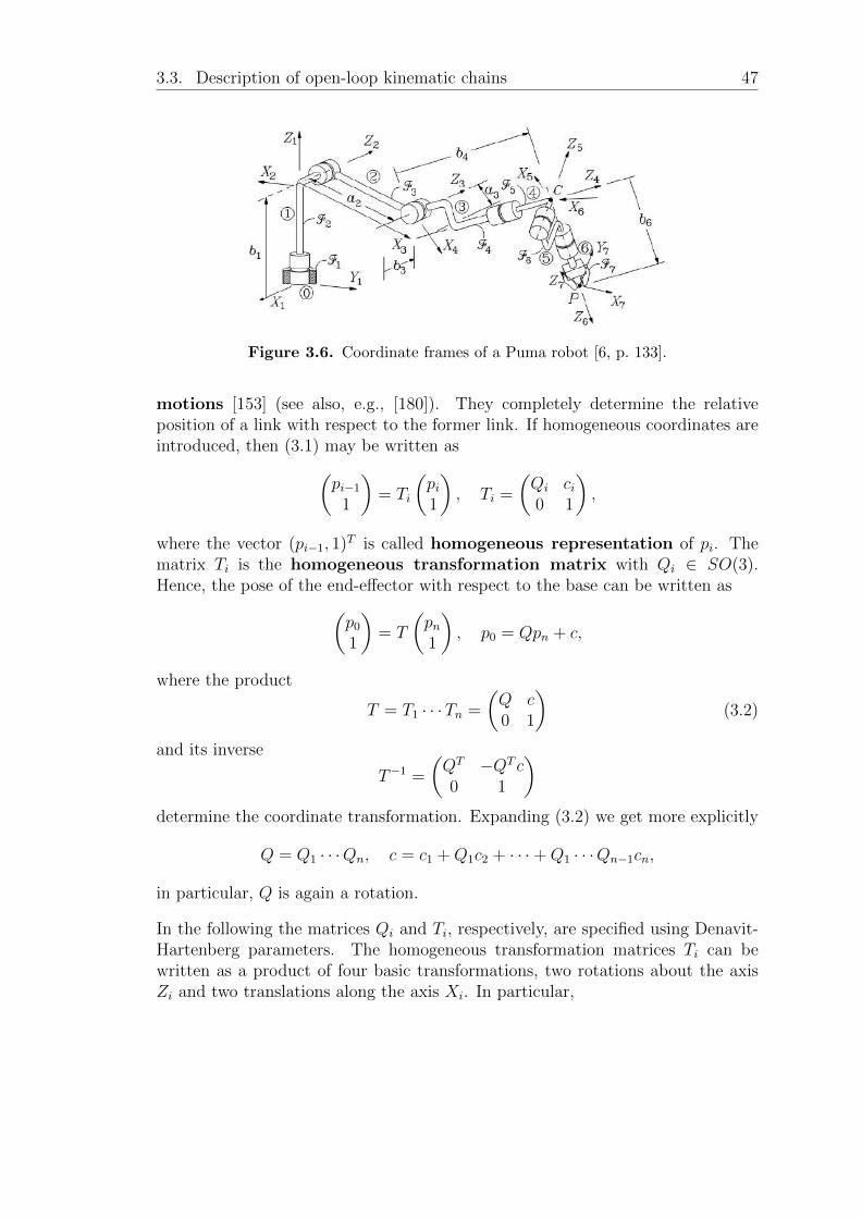
3.3. Description of open-loop kinematic chains 47
Figure 3.6. Coordinate frames of a Puma robot [6, p. 133].
motions [153] (see also, e.g., [180]). They completely determine the relativeposition of a link with respect to the former link. If homogeneous coordinates areintroduced, then (3.1) may be written as(
pi−1
1
)= Ti
(pi1
), Ti =
(Qi ci0 1
),
where the vector (pi−1, 1)T is called homogeneous representation of pi. Thematrix Ti is the homogeneous transformation matrix with Qi ∈ SO(3).Hence, the pose of the end-effector with respect to the base can be written as(
p0
1
)= T
(pn1
), p0 = Qpn + c,
where the product
T = T1 · · ·Tn =
(Q c0 1
)(3.2)
and its inverse
T−1 =
(QT −QT c0 1
)determine the coordinate transformation. Expanding (3.2) we get more explicitly
Q = Q1 · · ·Qn, c = c1 +Q1c2 + · · ·+Q1 · · ·Qn−1cn,
in particular, Q is again a rotation.
In the following the matrices Qi and Ti, respectively, are specified using Denavit-Hartenberg parameters. The homogeneous transformation matrices Ti can bewritten as a product of four basic transformations, two rotations about the axisZi and two translations along the axis Xi. In particular,

48 Chapter 3. Architecture
Ti = RotZiθi TransZidi TransXiai RotXiαi
=
ci −si 0 0si ci 0 00 0 1 00 0 0 1
1 0 0 00 1 0 00 0 1 di0 0 0 1
1 0 0 ai0 1 0 00 0 1 00 0 0 1
1 0 0 00 cαi
−sαi0
0 sαicαi
00 0 0 1
(3.3)
=
ci −sicαi
sisαiaici
si cicαi−cisαi
aisi0 sαi
cαidi
0 0 0 1
,
where ci = cos θi, si = sin θi and cαi= cosαi, sαi
= sinαi. Thus, denotingthe upper left 3 × 3-matrix of the rotational matrices in (3.3) by QZi
and QXi,
respectively,
Qi = QZi(θi)QXi
(αi) (3.4)
ci = QZi(θi)
ai0di
. (3.5)
The axis Zi is chosen to be the axis of actuation for joint i, i.e., the axis ofrevolution and the axis of translation, respectively, for the corresponding kinematicpairs. The Xi-axis is the common perpendicular to Zi−1 and Zi, directed from theformer to the latter; axis Yi is chosen to complete the coordinate system to be aright hand frame.
The used parameters αi, θi, di, and ai have a natural geometric meaning and arecalled the Denavit-Hartenberg parameters (short DH parameters) of a kine-matic pair [6] (see Fig. 3.7).
ai is defined as the distance between the axes Zi and Zi+1. Therefore, it is non-negative and called link length.
di is defined as the Zi-coordinate of the intersection of Zi with Xi+1. Its absolutevalue is the distance between the axes Xi and Xi+1 and is called the linkoffset.
αi is defined as the angle between Zi and Zi+1 measured about the positive direc-tion of Xi+1. It is called the twist angle between successive pair axes.
θi is defined as the angle between Xi and Xi+1 measured about the positive di-rection of Zi. This item is known as the joint angle.
If the ith pair is revolute, the joint angle θi is variable, whereas ai, di and αi areconstants. The former is termed joint variable (or joint coordinate, articularcoordinate) of the ith pair, in the following denoted by Θi; the constants are
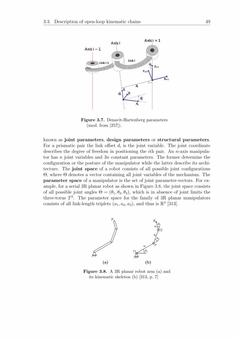
3.3. Description of open-loop kinematic chains 49
Figure 3.7. Denavit-Hartenberg parameters(mod. from [257]).
known as joint parameters, design parameters or structural parameters.For a prismatic pair the link offset di is the joint variable. The joint coordinatedescribes the degree of freedom in positioning the ith pair. An n-axis manipula-tor has n joint variables and 3n constant parameters. The former determine theconfiguration or the posture of the manipulator while the latter describe its archi-tecture. The joint space of a robot consists of all possible joint configurationsΘ, where Θ denotes a vector containing all joint variables of the mechanism. Theparameter space of a manipulator is the set of joint parameter-vectors. For ex-ample, for a serial 3R planar robot as shown in Figure 3.8, the joint space consistsof all possible joint angles Θ = (θ1, θ2, θ3), which is in absence of joint limits thethree-torus T 3. The parameter space for the family of 3R planar manipulatorsconsists of all link-length triplets (a1, a2, a3), and thus is R3 [313].
(a) (b)
Figure 3.8. A 3R planar robot arm (a) andits kinematic skeleton (b) [313, p. 7]

50 Chapter 3. Architecture
For a prismatic pair in the variable linear position Θi one has
Qi = QZi(αi), ci =
ai0
Θi
,
following from (3.4) and (3.5) with θi = 0. For a revolute joint in the variableangle position Θi, Qi and ci are derived directly from (3.3) by setting θi = Θi.Note that for prismatic pairs the matrix Qi is constant, while for revolute joints
c′i = QTi ci =
aidi sinαidi cosαi
(3.6)
is a constant vector. The detailed conventions of DH parameters might differslightly from the above by different authors, depending on the choice of the ref-erence axes and the way the angles and signs are defined. For further details see,e.g., [6, 57, 286].
3.3.2 Screw displacements
Another approach for the kinematic modeling of robot manipulators is to use suc-cessive screw displacements. In contrast to the Denavit-Hartenberg convention,the screw-based method uses a non-minimal parameter representation of the kine-matic chain. The method will not be discussed in detail, but a few notions areintroduced at this point, including the Plucker coordinates of a line. A compara-tive analysis of the kinematic modeling using Denavit-Hartenberg parameters andthe screw-based method is given by Rocha et al. [257].
A screw is a geometric entity representing both rotational and translational quan-tities. As stated in Chasle’s Theorem [6], a general spatial displacement of a rigidbody can be attained by a combination of a translation along an axis and a sub-sequent rotation about the same axis. The axis of action is called screw axis L.The axis combined with a scalar pitch, which relates translation and rotation iscalled a screw.
A convenient way to define any line in three-dimensional space is by using thePlucker coordinates of a line [6, Ch. 3].
Definition 3.3.1 (Plucker coordinates). Let x1 and x2 denote the position vectorsof two points X1 and X2 lying on a line L. Then the Plucker coordinates of Lare the entries of the 6-dimensional array γL, given by
γL :=
(x2 − x1
x1 × (x2 − x1)
). (3.7)
By setting
e :=x2 − x1
‖x2 − x1‖, n := x1 × e,

3.4. Separable (parallel) robots 51
equation (3.7) can be written in normalized Plucker coordinates as
γL = ‖x2 − x1‖(
en
), (3.8)
where e determines the direction of L and n its location.
The vector n can be interpreted as the moment of a unit force parallel to e andof line of action L. The six components of the Plucker array, the Plucker coor-dinates are not independent, since
e · e = 1, e · n = 0
hence, any line L has only four independent Plucker coordinates. Note further,that the Plucker coordinates are homogeneous coordinates (see, e.g., [275, Ch. 6]for details).
A rigid-body motion may now be described by 8 scalars, of which six parametersare independent. These are the four independent components of the Plucker coor-dinates defining the screw axis, the amount of linear translation along the axis andthe rotation angle about the axis (amplitude). A motion described by these sixparameters is called screw displacement. Thus, a general screw displacementfor a rigid body may be given by Rodrigues’s formula
x2 = R(φ)x1 + d(d0),
where xi = (xix, xiy, xiz)T , Q(φ) is the rotation matrix corresponding to the ro-
tation φ about the screw axis and d(d0) is a displacement vector correspondingto the translational distance d0 along the screw axis [96] (see Fig. 3.9). Thus, ascrew given by the screw parameters φ and d0, can be used to describe the poseof a rigid body relative to a referential system [257].
An instantaneous rigid-body motion relative to a referential system is called aninstantaneous screw (or twist). It is defined by the instant screw axis L′,a pitch p′ and an amplitude ‖ω‖, which represents the magnitude of the angularvelocity. The instantaneous screw may alternatively be defined by six independentscalars, the three components of its angular velocity ω and the three componentsof the velocity v of an arbitrary point X1. If the pitch equals zero, the twist is apure rotation, whereas the twist is a pure translation for a pitch equal to infinity.(for further details see, e.g., [6]). So, screw theory associates physical meaningto a geometric entity by expressing (linear and angular) velocities as twists andforces/torques as wrenches [257]. Further discussion of instantaneous motion ispresented in Chapter 6.
3.4 Separable (parallel) robots
An important class of serial manipulators are so-called decoupled manipulators(see Fig. 3.10). In a decoupled manipulator the last three joints have intersecting
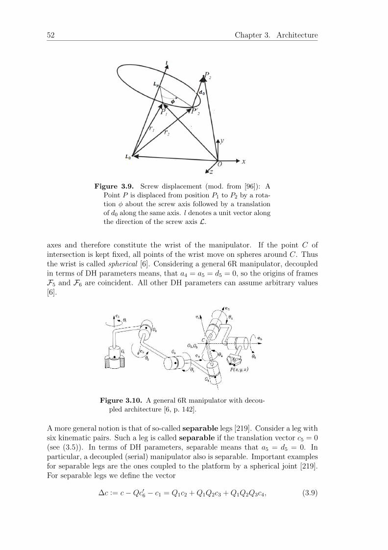
52 Chapter 3. Architecture
Figure 3.9. Screw displacement (mod. from [96]): APoint P is displaced from position P1 to P2 by a rota-tion φ about the screw axis followed by a translationof d0 along the same axis. l denotes a unit vector alongthe direction of the screw axis L.
axes and therefore constitute the wrist of the manipulator. If the point C ofintersection is kept fixed, all points of the wrist move on spheres around C. Thusthe wrist is called spherical [6]. Considering a general 6R manipulator, decoupledin terms of DH parameters means, that a4 = a5 = d5 = 0, so the origins of framesF5 and F6 are coincident. All other DH parameters can assume arbitrary values[6].
Figure 3.10. A general 6R manipulator with decou-pled architecture [6, p. 142].
A more general notion is that of so-called separable legs [219]. Consider a leg withsix kinematic pairs. Such a leg is called separable if the translation vector c5 = 0(see (3.5)). In terms of DH parameters, separable means that a5 = d5 = 0. Inparticular, a decoupled (serial) manipulator also is separable. Important examplesfor separable legs are the ones coupled to the platform by a spherical joint [219].For separable legs we define the vector
∆c := c−Qc′6 − c1 = Q1c2 +Q1Q2c3 +Q1Q2Q3c4, (3.9)
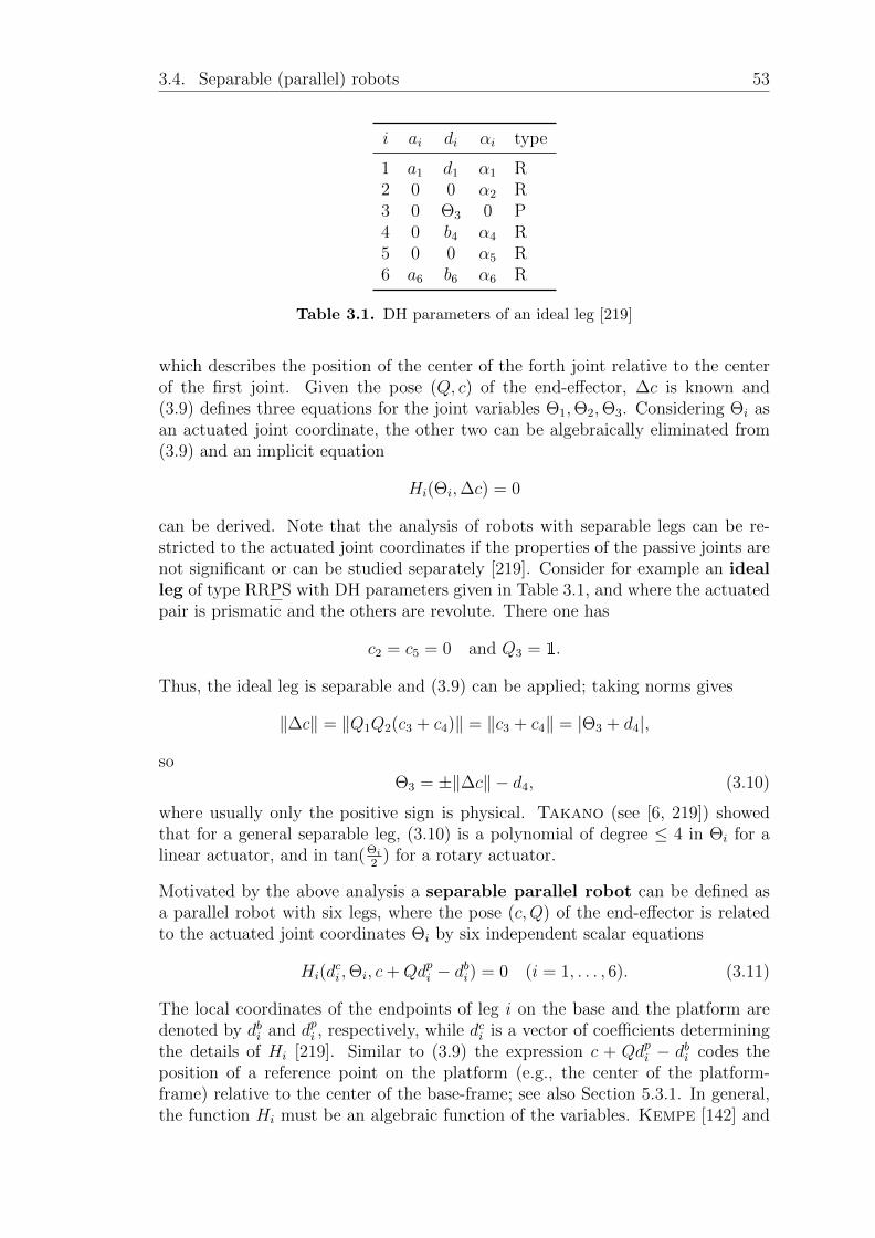
3.4. Separable (parallel) robots 53
i ai di αi type
1 a1 d1 α1 R2 0 0 α2 R3 0 Θ3 0 P4 0 b4 α4 R5 0 0 α5 R6 a6 b6 α6 R
Table 3.1. DH parameters of an ideal leg [219]
which describes the position of the center of the forth joint relative to the centerof the first joint. Given the pose (Q, c) of the end-effector, ∆c is known and(3.9) defines three equations for the joint variables Θ1,Θ2,Θ3. Considering Θi asan actuated joint coordinate, the other two can be algebraically eliminated from(3.9) and an implicit equation
Hi(Θi,∆c) = 0
can be derived. Note that the analysis of robots with separable legs can be re-stricted to the actuated joint coordinates if the properties of the passive joints arenot significant or can be studied separately [219]. Consider for example an idealleg of type RRPS with DH parameters given in Table 3.1, and where the actuatedpair is prismatic and the others are revolute. There one has
c2 = c5 = 0 and Q3 = 1.
Thus, the ideal leg is separable and (3.9) can be applied; taking norms gives
‖∆c‖ = ‖Q1Q2(c3 + c4)‖ = ‖c3 + c4‖ = |Θ3 + d4|,
soΘ3 = ±‖∆c‖ − d4, (3.10)
where usually only the positive sign is physical. Takano (see [6, 219]) showedthat for a general separable leg, (3.10) is a polynomial of degree ≤ 4 in Θi for alinear actuator, and in tan(Θi
2) for a rotary actuator.
Motivated by the above analysis a separable parallel robot can be defined asa parallel robot with six legs, where the pose (c,Q) of the end-effector is relatedto the actuated joint coordinates Θi by six independent scalar equations
Hi(dci ,Θi, c+Qdpi − dbi) = 0 (i = 1, . . . , 6). (3.11)
The local coordinates of the endpoints of leg i on the base and the platform aredenoted by dbi and dpi , respectively, while dci is a vector of coefficients determiningthe details of Hi [219]. Similar to (3.9) the expression c + Qdpi − dbi codes theposition of a reference point on the platform (e.g., the center of the platform-frame) relative to the center of the base-frame; see also Section 5.3.1. In general,the function Hi must be an algebraic function of the variables. Kempe [142] and

54 Chapter 3. Architecture
Freudenstein & Roth [82] showed, that every algebraic curve can be realizedby a closed kinematic chain with a single degree of freedom. Therefore, it isconceivable that, in principle, any set of algebraic functions Hi can be realized inthis way by a sufficiently complex leg.
Depending on the considered class of robots, (3.11) can be formulated more specif-ically [219]. A Gough platform (see Fig. 3.11) with six ideal legs of type RRPScan be characterized by the relation
‖c+Qdpi − dbi‖2 − (li + Θi)2 = 0, (3.12)
where li denotes the parts of the ith leg of fixed length (see also Ex. 5.3.1). Note,that in a general Gough platform neither the base nor the platform need to beplanar (see Fig. 3.5).
Figure 3.11. Scheme of a Gough platform (mod. from [196]).
Separable parallel robots with legs of type PRRS are called active wrist orhexaglide [111] and satisfy equations of the form
‖c+Qdpi − dbi −Θiu‖2 − l2i = 0. (3.13)
Similarly, so-called Hexa robots [243], i.e., separable parallel robots with legs oftype RRRS, satisfy equations of the form
‖c+Qdpi − dbi − (cos Θi)u− (sin Θi)v‖2 − l2i = 0. (3.14)
Summarizing, we can say that a large, practically relevant class of parallel robotscan be completely described by (3.11) (and the special cases (3.12), (3.13), and(3.14), respectively), together with the six equations
(QTQ)ik = δik =
1 if i = k,
0 otherwise,(3.15)
and the orientation constraintdetQ = 1. (3.16)

Chapter 4
Geometry
4.1 Introduction
The geometry of a robot mechanism treats questions about numerical dimensionsof the robot parts, limits on lengths and angles, interferences between legs (inparallel manipulators) or the accessible workspace. For coding the pose (i.e.,position and orientation) of the end-effector of a robot, generalized coordinatess are used. The equation of state
F (s,Θ) = 0 (4.1)
relates the pose to the joint configuration (or posture) Θ, which describes thecombined positions and orientations of all links and the end-effector (or mobileplatform) [219]. The pairs (s,Θ) satisfying (4.1) are called states. A measure-ment vector y contains the values obtained by internal sensor measurements andis related to the joint configuration Θ by the measurement equation
y = PΘ, (4.2)
where P is a matrix with exactly one 1 per row and zeros elsewhere, which rep-resents the projection to the vector of measured joint variables. The equation ofstate contains all information about the geometry of the measured joints and theend-effector. For finding limits of ranges on joint variables, global size constraintsfor a robot, or inequality constraints for ensuring the absence of interferences be-tween different legs, however, more detailed information is necessary about how therobot is built; the equation of state does not cover these items. In the generic case,i.e., if the implicit function theorem is applicable, it is ensured by the dimensionalconstraint
dim y ≤ dim s+ dim Θ− dimF, (4.3)
that the measurements contain enough information to determine a local change ofpose [219].
If equality holds in (4.3), the robot is called minimally instrumented robot[219]. Typically, this is the case if the actuators are instrumented and the passive
55

56 Chapter 4. Geometry
joint variables are eliminated explicitly from the mathematical model, i.e., whenΘ is reduced to the n actuated joint variables. Thus, in the case of independentgeneralized coordinates, y = Θ and dimF = dim s. For a minimally instrumentedserial robot, the equation of state may be written explicitly as
s = F (Θ), (4.4)
and is obtained by writing relation (3.2) in terms of the generalized coordinates.For a minimally instrumented separable parallel robot, the equation of state isgiven by equation (3.11). In particular, for a Gough platform, (4.1) has the explicitform
Θ = F (s). (4.5)
It is obtained by writing (3.12) in terms of the generalized coordinates.
4.2 Sets and Maps
For the main types of geometric problems that typically arise in kinematics it isconvenient to define several sets and the corresponding maps, which are shownin the following commutative diagram. The descriptions are given according toWampler & Sommese [313].
Y MJoo K //
πM
J
K
##
O
Y × P π2//
π1
OO
P O × Pπ3oo
π4
OO
The sets are described as follows:
Y denotes the input or joint space of the mechanism. Its coordinates are thejoint variables Θ (or y = PΘ) (which are typically controlled by actuators).
O denotes the output or operational space of the mechanism. Its coordinatesare the poses s of the end-effector.
P denotes the parameter space of a family of mechanisms (e.g., the set of all 6Rserial robots). It is the set of parameters necessary to describe the geometryof the joints in each link. Thus, each point in P corresponds to a specificmechanism with specified link lengths, etc.
M denotes the mechanism space, M ⊆ Z × P , where Z = SE(3)n−1 (or, fora planar mechanism family, Z = SE(2)n−1) is the link space for an n linkmechanism. M describes all possible configurations of a mechanism for allpossible parameters. So, each point (z, p) ∈ M represents a specific mech-anism p ∈ P in one of its assembly configurations z ∈ Z. The mechanismspace M of a mechanism family is the subset of Z×P that satisfies the jointconstraints. Thus, M characterizes a family of mechanisms, e.g., the familyof spatial 6R serial robots.

4.3. Generalized coordinates 57
Further, the following three maps are defined on M :
The input map J : M → Y extracts the input values from M .
The output map K : M → O extracts the output values from M .
The projection πM : M → P extracts the parameters from M . It is the naturalprojection operator on Z × P restricted to M , given by πM : (z, p) 7→ p.
The above diagram is completed by defining J = (J, πM) and K = (K, πM) andthe associated natural projections πi for i = 1, . . . , 4. Further, it is useful to definethe inverses of the input/output maps,
J−1(y) = (z, p) ∈M | J(z, p) = yK−1(s) = (z, p) ∈M | K(z, p) = s,
which apply to a whole mechanism family, as p ∈ P is not fixed. If one wants toaddress only one specific mechanism, the inverses of J and K have to be considered.In analysis problems, typically a specific mechanism p∗ ∈ P is given and thebasic problems may be formulated using the above definitions. For example, theforward kinematics problem (see Chapter 5) is to find output (i.e., pose(s))s ∈ O of a manipulator which corresponds to a given input-vector of joint variablesy∗ ∈ Y for a given mechanism p∗ ∈ P ,
FKP(y∗, p∗) = K(J−1(y∗, p∗)). (4.6)
The inverse kinematics problem goes from output to input and is to find thevector(s) of joint variables y ∈ Y that correspond to a given pose s∗ ∈ O for agiven mechanism p∗ ∈ P ,
IKP(s∗, p∗) = J(K−1(s∗, p∗)). (4.7)
For a more detailed discussion of geometric problems arising in kinematics see[313, Ch. 4].
4.3 Generalized coordinates
The generalized coordinates code the pose of the end-effector relative to thebase. E.g., for a (serial) robot manipulator consisting of N rigid bodies, 6Ncoordinates are required to specify the position and orientation of all the bodiesrelative to a coordinate frame. But, because some of the links are joined together,there is a number of constraint equations which establish relationships betweensome coordinates. Therefore, the 6N coordinates can be expressed as functionsof a smaller set s of coordinates, that are all independent. The coordinates ofs are known as generalized coordinates; the joint variables Θ form a set ofgeneralized coordinates [280].

58 Chapter 4. Geometry
There are multiple ways of choosing the set of generalized coordinates; in principle,their choice is a matter of convenience. The displacement vector is usually givenin Cartesian form, although other parameterizations, e.g., the dual quaternionparameterization of Study [288] (see, e.g., [123]) are discussed in the literature(e.g., [122, 124, 235, 250, 310]). For a definite description, the vector of generalizedcoordinates s is defined as
s =
(rc
),
where c is the position of a specific point of the end-effector relative to the base,and r encodes the rotation Q = Q[r] in such a way, that (3.15) and (3.16) holdfor all admissible r. The rotation may be written in terms of a convenient param-eterization. A common used one for three-dimensional rotations is the so-calledEuler angles parameterization. According to Euler’s rotation theorem, everyrotation may be described using three angles, frequently denoted by ϕ, θ, ψ. Therotation Q may be achieved by composing three elemental rotations about cer-tain axes of the coordinate frame. There are many significantly different ways ofdefining the Euler angles, depending on the posed problem. One highly used rep-resentation is pitch-roll-yaw (see, e.g., [132, 133, 289]); for further information onEuler angles and other Euler angles set conventions see, e.g., [57, 216, 286]. Otherways for parameterizing the rotation Q[r] are the quaternion parameterization,or more redundant parameterizations involving components of Q and additionalorthogonality constraints relating these. Taking for r simply the components ofQ (restricted by (3.15) and (3.16)) produces the simplest but most redundantparameterization [219].
Using a trigonometric parameterization in terms of angles (e.g., Euler angles),its interpretation depends on a fixed coordinate system. Further, additional sin-gularities for certain angle combinations are introduced. Therefore, the quater-nion parameterization is a numerically more convenient and singularity-freeparameterization of rotations. Most of the following statements about quaternionrepresentation, further explanations, and proofs can be found in Neumaier [220].
Theorem 4.3.1 (Quaternion parameterization). Let r ∈ R3 with rT r ≤ 1 andr0 =
√1− rT r, and let X ∈ R3×3 be a skew-symmetric matrix of the form
X(r) :=
0 −r3 r2
r3 0 −r1
−r2 r1 0
.
Then the matrixQ[r] := 1 + 2r0X(r) + 2X(r)2, (4.8)
is a rotation. Conversely, every rotation Q has the form Q = Q[r] for some r ∈ R3
with rT r ≤ 1.
Proof. See Neumaier [220].
Using the fact thatX(r)2 = rrT − rT r1,

4.3. Generalized coordinates 59
(4.8) can be expanded to
Q[r] = 1 + 2 ·R, R :=
−r22 − r2
3 r1r2 − r0r3 r1r3 + r0r2
r1r2 + r0r3 −r21 − r2
3 r2r3 − r0r1
r1r3 − r0r2 r2r3 + r0r1 −r21 − r2
2
. (4.9)
Relation (4.9) can be written in homogeneous form by
Q[r0, r] = 1 +2
r20 + r2
·R, (4.10)
with r0 ∈ R, r ∈ R3 not both zero. Further, (4.10) reflects the fact that SO(3)has the structure of a projective 3-space (see, e.g., [178]). Since Q[r0, r] satisfies
Q[r0, r] = Q[λr0, λr], λ 6= 0,
i.e., scaling r0 and r by the same nonzero factor does not change the rotationmatrix, (r0, r) may be normalized to
r0 ≥ 0, r20 + r2 = e (e > 0 fixed).
Thus, the quaternion parameterization of rotations given in (4.8) may be writtenas Q = Qe[r] with
Qe[r] = 1 +2
e·R, (4.11)
where r ∈ R3, r2 ≤ e and r0 =√e−
∑3i=1 r
2i . For e = 2, the factor 2
ecan be
deleted and Q2[r] can be computed with only 15 additions, 9 multiplications anda square root. However, the standard scaling in the literature has e = 1, whichmakes the computation of (4.11) more expensive, but saves the factor e−1/2 in themultiplication rule (4.13) below. Different normalization conventions may be usedas well, such as, e.g., r0 = 1 or r2
0 + r2 = 2r0, which work well for rotations by alimited angle [219].
For r2 = e, we get r0 = 0 and Qe[r] = Qe[−r]; thus, antipodal vectors r oflength
√e are identified in the quaternion parameterization. This reflects the non-
Euclidean structure of SO(3) and has to be taken into account when constructingsmooth motions joining two poses involving a small r0 but nearly opposite r [219](see, e.g., [10, 254, 279, 342]). Geometrically, Q[r] describes a rotation around the
vector r by the angle Φ = arcsin( |r|√e).
Independent of the parameterization, the product of rotations again is a rotation.This fact implies the existence of a product formula
Qe[r]Qe[s] = Q[r ⊕ s], (4.12)
where ⊕ denotes a parameterization dependent, non-commutative but associativebinary operation ⊕. One elegant way to derive (4.12) is using quaternions. Aquaternion is a 4× 4 matrix of the form
U(r0, r) :=
(r0 rT
−r r01 +X(r)
),
for r0 ∈ R, r ∈ R3. Quaternions are used for proving the following theorem, whichprovides the product formula for the quaternion parameterization (4.11).

60 Chapter 4. Geometry
Theorem 4.3.2 (Product formula for rotations in quaternion parameterization).Let r2 ≤ e,s2 ≤ e. Then there exists a product formula (4.12), where
r ⊕ s := ±e−1/2(s0r + r0s+ r × s), (4.13)
for r0 =√e− r2, s0 =
√e− s2 and the sign chosen such that ±(r0s0 − r · s) ≥ 0.
Further,Qe[r]
−1 = Qe[r]T = Qe[−r], r ⊕ (−r) = 0.
Proof. See Neumaier [220].
Applications for the quaternion representation are given in, e.g., [258, 312], whereit is used for the forward displacement analysis of spherical parallel manipulators.Wampler [310] used Study’s soma coordinates, which are, except for a factorof 1/2 identical to dual quaternions, for the forward displacement analysis of ageneral 6-SPS Stewart platform.
4.4 Workspace
Generally, the workspace of a mechanism is a region of points that can be reachedby a reference point on the manipulator extremity [44]. The end-effector cannotreach every pose, due to its mechanical architecture (e.g., link-lengths) or tech-nological constraints, such as limits on the joint motions. For both serial andparallel manipulators, the motions can be restricted by limits on the passive jointsor limitation due to the actuators. For parallel robots, there are perhaps boundson the angles between legs and platforms, which are chosen such that the legs donot interfere with each other within these limits. All these restrictions are takeninto account in the modeling process. In the most general case, the constraintsare defined by a vector of constraint inequalities,
C(s,Θ) ∈ C, (4.14)
where C is a simple set, defined by lower and/or upper bounds on the componentsonly [219]. The set of states (s,Θ) satisfying the equation of state (4.1) and (4.14)is a manifold. If the dimension of this manifold is d, then the robot is said tohave d degrees of freedom [219]. The manifold can be connected or disconnected;in the latter case, the workspace is split into separate components, which meansthat the robot can be assembled in different, equivalent ways. Here, only thecomponent S containing the nominal assembling position is of interest. The sixdimensional manifold S is called the state space of the mechanism [219]. The setof all attainable poses of the end-effector is called complete workspace. In caseof a 6 d.o.f. manipulator it is the 6D-workspace W ⊂ SE(3), which is describedby the projection
W = s | (s,Θ) ∈ S

4.4. Workspace 61
of the state space to the space of possible poses. Recall that s consists of a vectorc, representing the coordinates of a specific point on the end-effector, and of avector r, whose components define the end-effector’s orientation. Thus, W canalso be written as
W = (c, r) | c ∈ Wc ⊆ R3; r ∈ R3 s.t. Q[r] ∈ Wr ⊆ SO(3),
where Wc and Wr denote the maximal three-dimensional reachable position andorientation workspaces, respectively. Thus, Wc(r) is the position workspace un-der constant orientation Q[r], and Wr(p) the orientation workspace underconstant position c [134].
The 6D-workspace contains all poses of the end-effector which are realizable bythe actuators within given constraints. The visualization of six dimensions is lim-ited, hence workspace problems generally only involve some projection of the 6D-workspace; but note, that planning problems may involve the full 6D-workspace.Problems which consist of finding the extremal values of one of the pose parametersare known as one-parameter problems, while three-parameter problems as-sume nominal constraints on three of the joint variables; e.g., they may have afixed value or must lie within given ranges. For one-parameter problems, a worstcase analysis is required, therefore these are global optimization problems. Thesehave never been fully investigated [219].
To formulate constraints on the pose, the positioning and orientational part of s (cand r, respectively), are treated separately. The robot has to work in an environ-ment of given size. Thus, constraints on the position c are generally simple boundsresulting from this need. Constraints on the orientation r are usually expressedby constraints on the values of some angles. However, quaternion parameters caneasily be used to encode geometric constraints. Consider the parameterizationQ = Qe[r], given by (4.11). According to Neumaier [219], the constraints
r2 ≤ e
2(1− cosα),
and equivalently,
r20 ≥
e
2(1− cosα)
limit the rotation to an angle |θ| < α around its axis. Further, the constraints
r21 + r2
2 ≤ r23 tan2 α,
and equivalently,
r20 +
r23
cos2 α≥ 1
limit the rotation axis to a circular cone with half opening angle α around theZ-axis. In the same way,
r21 tan2 α ≤ r2
2 + r23,
and equivalently,
r20 +
r21
cos2 α≥ 1
62 Chapter 4. Geometry
keep the rotation axis away from a circular cone with half opening angle α aroundtheX-axis, without restricting it in theXY -plane. General homogeneous quadraticinequalities do the same for other preferred or avoided orientations.
Due to the six dimensions of the workspace, a graphical illustration of the robotworkspace is difficult to provide. In contrast to serial manipulators, for parallelrobots having more than 3 d.o.f. there exists no such graphical representation.Consider for example a serial manipulator with 6 d.o.f. with a concurrent axiswrist. It may be represented by the 3D-volume reachable by the center of thewrist, which illustrates the translations. Two of the rotational degrees of freedommay then be represented by the surface that may be reached by the extremity ofthe end-effector [198]. The graphical representation of the workspace of a parallelrobot is possible only for robots with at most 3 d.o.f. Workspace representationfor robots with n > 3 d.o.f. will only be possible, if n − 3 pose parameters arefixed. This assumption can be taken, because in many situations the platformeither operates with a fixed orientation or rotates about a fixed point. Machoet al. [174] provide a new software tool which computes and visualizes differentworkspace-types of parallel manipulators, depending on the user chosen variables,onto which the workspace shall be projected. Depending on the choice of the poseparameters and the constraints imposed on these, different types of workspace willbe obtained and impose certain types of three-parameter problems; for example,for a general Stewart platform, a total of twenty different slices of the 6D workspacecan be obtained [21].
The typically relevant types of workspace are ([198]):
constant orientation workspace or translation workspace: all possible po-sitions of a fixed point C at the robot that can be reached with a givenorientation,
orientation workspace: all possible orientations that can be reached given thatC is in a fixed location,
total orientation workspace: all the locations of C that may be reached withall the orientations among a set defined by ranges on the orientation angles,
dextrous workspace: important special case of the total orientation workspace,which contains all locations of C for which all orientations are possible,
maximal workspace or reachable workspace: all the locations of C that maybe reached with at least one orientation of the end-effector.
But other specific workspace definitions may be useful for certain tasks; e.g.,Bonev & Gosselin [25] give a fast algorithm for the so-called constant-torsionworkspace of symmetrical spherical parallel mechanisms and presents a methodol-ogy for the analytical determination and representation of the workspace bound-aries.

4.4. Workspace 63
The corresponding three-parameter problems to the above described workspacetypes are listed below in increasing order of complexity [219].
Constant orientation workspace: Find the set of positions c such that s ∈ Wfor a given orientation r.
Orientation workspace: Find the set of orientations r such that s ∈ W for agiven position c.
Total orientation workspace: Find the set of positions c such that s ∈ W forall r ∈ r for a given set of r of desired orientations.
Dextrous workspace: Find the set of positions c such that s ∈ W for all r ∈ r,where r consists of all meaningful choices of orientations (in particular, forEuler angles r is the range [0, 2π]2× [0, π], and for quaternions it is the unitball).
Maximal workspace: Find the set of positions c for which there exists at leastone orientation r such that s ∈ W .
4.4.1 Workspace for parallel robots
Constant orientation workspace
Three-parameter problems are constraint satisfaction problems of the coveringtype, and therefore usually expensive to solve. But if only limits on the actuatedjoints are considered, the computational effort can be significantly reduced. Forexample, the constant orientation workspace for separable parallel robots is theintersection of six circular rings and the workspace boundaries are given by circulararcs, and may be computed in a few milliseconds by an algorithm provided byGosselin [89]. In the presence of constraints on joint limits in the passive joints,or possible leg interference, the problem becomes more complex [186]. The interiorof the constant orientation workspace of a Gough-type platform was computedwith interval methods by Merlet [193].
An alternative approach for accurate and computationally effective calculationof the constant orientation workspace of a constrained parallel manipulator wasgiven by Shah et al. [276], using CAD modeling software. The used geometricprogramming methods (constraint analysis and Boolean volumetric operations),could potentially be much more insightful, efficient and accurate compared toconventional parameter sweep methods.
Orientation workspace
The computation and visualization of the orientation workspace turn out to bemore difficult, due to more complex equations and the difficulty of representing

64 Chapter 4. Geometry
orientations intuitively [21]. A possibility is to hold the orientation angles fixed[188], or to let the three angles vary [236]. But all methods rely on some sort ofdiscretization and therefore, produce incomplete or less accurate output in somesituations [21]. Jiang & Gosselin [133] gave a fast method providing appealingvisualizations of the orientation workspace of a Gough-Stewart platform, but me-chanical limits in the passive joints are neglected; thus, the computed workspaceis an overestimation of the true workspace. Further, some methods only computethe connected component of the workspace which is achievable from a pre-definedinitial assembly configuration [296].
Cao et al. [38] present a discretization method based on half-angle transformationand the inverse kinematics solution for computing the orientation workspace of aGough-Stewart platform with similar semi-symmetrical hexagon base and plat-form. The method also takes limitations of active and passive joints and linkinterference into account.
Another numerical approach was given by Yang & Chen [336] for the orientationworkspace analysis of a 3 d.o.f. spherical manipulator, using a novel partitionscheme for dividing the sphere D3 to which SO(3) can be mapped, into finiteelements with equal volume.
According to Bohigas et al. [21], a proposed method for workspace computationshould ideally be complete, accurate and as general as possible. The property ofbeing complete refers to the ability of finding all connected components of theworkspace, rather than obtaining just one achievable from a recent configuration.Further, a precise representation of the workspace volume and of any motion bar-riers in the interior of the volume is required with high accuracy. Finally, everypossible workspace slice that can be obtained by fixing three of the pose parame-ters, should be determined. A unified method satisfying the previous requirementswas given in [21], valid for Stewart platforms consisting of base and platform ofarbitrary geometry, connected by six legs of type UPS. First, a system of equationsis formulated, defining the boundary ∂W of the workspace W . Then, an iterativeprocedure based on linear relaxations is used to isolate slices of such boundaryexhaustively at the required solution. In particular, a system of 33 equations in39 variables represents the general 6D-workspace, using the joint variables andconstraints introduced by the mechanical limits on all joints. The boundary ∂Wis then obtained by adding an additional equation, representing the property thata point lies on ∂W , whenever any of the active or passive joints reaches a mechan-ical limit. Thus, the ∂W has one dimension less then mathcalW itself. However,it is still hard to compute the boundary exhaustively; but by setting three vari-ables to a constant value, arbitrary two-dimensional slices of the boundary can beobtained. The algorithm for solving the system of equations numerically is basedon a linear relaxation paradigm (described by Porta et al. [247]), starting withalgebraizing the equations into a canonical form. An initial box containing all thesolutions is computed, and then all boundary points at the desired resolution areisolated using a branch-and-prune method. Results with computations times ofabout one minute for computing the constant position and the constant orientation

4.4. Workspace 65
workspace are provided. However, possible leg interferences are not taken into ac-count. The proposed method shows potential of being able to cope with additionalconstraints, like singularity-avoidance or leg-leg collisions, but further work seemsrequired to provide a formulation ensuring an acceptable computational effort.
Maximal workspace
The most difficult task is the calculation of the maximal workspace, which maytake hours of computation time for manipulators with large ranges for certain jointvariables [191].
A complete analysis of the reachable workspace of spatial Gough-Stewart platformswith planar base and platform was given for the first time in 2006 by Pernkopf& Husty [236].
Jin et al. [134, 135] found optimal dimensions for the maximal 6D-workspace ofa 3RPPS parallel manipulator, using an approach of finite-partitioning of SE(3)(based on [336]). The workspace optimization presented there is valid, but com-putational expensive, due to the large number of sampling features.
An algorithm for computing the reachable workspace of symmetric spatial parallelmanipulators was proposed by Zhao et al. [346, 347], who investigated the anal-ogous symmetry properties between the workspace and the mechanism structure.It has been proven, that the symmetry group (which for a polygon V in the planeconsists of all motions φ for which φ(V ) = V ) of the kinematic chain structure ofthe end-effector must be a subgroup of that of the end-effector. The computationaleffort may be reduced significantly, because only a reduced part of the workspaceneeds to be investigated; in particular, if the order of the symmetry group of themechanism structure is n, then the search area can be reduced to 1
nof the initial
one.
Further results
An analytic solution for the reachable workspace of axially symmetric hexapodswas given by Agheli & Nestinger [1], based on a decomposition of the mecha-nism into three intersecting modified four-bar mechanisms. The method is exten-sible to other types of workspaces and manipulator geometries.
An overview of workspace determination for several types of parallel manipula-tors, e.g., for planar manipulators, 3-UPU-manipulators, and the general 6-UPSmanipulator, are given by Merlet [198]. For other types of parallel manipu-lators, specific research has been done; for example Cervantes-Sanchez et al.[46] present a methodology for the determination of the workspace for 5R sphericalsymmetric manipulators or Hay & Snyman [105] a numerical multilevel optimiza-tion method for determining the dextrous workspace of a 3 d.o.f. planar parallelmanipulator.
66 Chapter 4. Geometry
Kotlarski et al. [148] present a method to enlarge the useable workspace, i.e., thesingularity-free workspace, guaranteeing a certain achievable accuracy for a givenactuator resolution. The method is based on interval analysis and is operationalfor planar parallel manipulators with kinematic redundancy, realized by adding atleast one actuated (prismatic) joint to one kinematic chain. Results show, that anadditional (prismatic) actuator significantly increases the useable workspace.
As mentioned before, a constraint which enforces limitation on the workspace is apossible self-collision, i.e., the collision between the legs of the robot, and, even-tually with the base or the platform. Collision detection may be formulated as aconstrained optimization problem in which distance between the legs is minimized.But there is no need to compute an exact value of the minimum, it is enough toshow whether it is lower or greater than a given value. Merlet & Daney[204] present an algorithm based on interval analysis, which exhibits an efficientleg interference check for 6 d.o.f. Gough-platforms, where the legs are modeledas finite cylindrical elements. The algorithm allows to detect an interference ina given workspace volume. Remaining problems are to determine the maximalinterference-free workspace or the design parameters so that a given workspacewill be interference free [204].
4.4.2 Workspace for serial manipulators
The determination of the workspace volume for serial manipulators is easier thanthe computation for parallel mechanisms. Consider for example a 3R planar ma-nipulator. There, the reachable workspace problem is to find the boundaries ofthe real working volume of the given robot with design parameters p∗ ∈ P , whichcan be accomplished by computing the singularity surface
S∗p = Θ ∈ TR3 | rank ∂ΘK3R(Θ, p∗) < 3,
where T 3R denotes the set of real joint angles, i.e., the joint space consisting of
all possible (real) joint angles Θ = (Θ1,Θ2,Θ3); in absence of joint limits, T 3
is the three-torus. K3R(Θ, p∗) denotes the forward kinematics map (cf. Section4.2) restricted to the set of parameters for given parameters p∗ for the robot.Then ∂ΘK3R denotes the 3 × 3 Jacobian of K3R with respect to the joint angles.The boundaries of the reachable workspace are contained in the image of thesingularities [313]. Guo et al. [97] present a complete classification and workspacecomposition of 3R planar manipulators based on the characteristics chart method.
For serial manipulators, the robot manipulator structure can be divided into twoseparate groups. The regional structure consists of the arm moving the end-effectorin a desired position; the orientation structure contains the link(s) rotating theend-effector to a desired orientation. Therefore, the positioning and orientationproblem can be discussed separately. Gupta & Roth [98] have presented somevaluable concepts regarding the workspace of manipulators. Different solutionapproaches for workspace calculations are possible, e.g., algebraic and geometricapproaches [42, 43, 300], continuation [136], heuristic methods [335], or single- and

4.4. Workspace 67
multi-objective optimization [16, 45, 226]. In particular, for 3R manipulators agreat number of publications can be found, due to their importance in industrialapplications. So Zein et al. [343] present a classification of 3R manipulators withat least one DH parameter equal to zero, based on the topology of the workspace.A characterization of the workspace boundary of 3R manipulators can be found in[272]. Ottaviano et al. [225] characterize workspace topologies of 3R industrialmanipulators by a level-set reconstruction; the proposed algebraic expressions areuseful to classify industrial 3R manipulators. Further, conditions for avoiding sin-gularities in the workspace are identified. Recently, a fast algorithm for numericalcomputation of the workspace has been presented by Shi et al. [277]. It is basedupon the singularity analysis of a manipulator. The algorithm is operational forserial manipulators with up to six revolute joints.
Since workspace quality and quantity have become most important performanceindices [135], the workspace of a robot manipulator is an important criterion for theoptimal design of the mechanism. Further, the property of being singularity-freeis a crucial aspect of workspace analysis (see Chapter 8).
4.4.3 Related problems
An associated problem to workspace determination is to define a geometrical ob-ject (e.g., a cube or a sphere) and determine the largest such object enclosed in theworkspace of the robot (see also section 8.3.1). For the Gough-Stewart platformof type MSSM (Maximal Simplified Symmetric Manipulator, see [198]), Jiang& Gosselin [132] provided an iterative algorithm for determining the maximalsingularity-free sphere in the orientation workspace (see Fig. 4.1). The problem isto find the point on the singularity surface which is closest to a reference orien-tation; the distance of this point to the reference orientation then is taken as theradius of the maximal singularity-free sphere.
Chablat et al. [51] present an interval-analysis based algorithm for 3 d.o.f.parallel manipulators to determine the largest cube (or, with some parameter-modifications the largest sphere or other regular shaped object) enclosed in thedexterous workspace. [52] present the square workspaces of two specific 3 d.o.f.manipulators. An algorithm which is able to verify (very quickly) whether anarbitrary trajectory (or surface or volume) lies entirely within the workspace wasproposed by Merlet [194]. The algorithm is based on interval arithmetic andtherefore provides the validity of a trajectory (surface/volume) in a guaranteedmatter. Further details about the singularity-free workspace are presented inChapter 8.
Another problem is to verify the reachability of a planned workspace; inparticular, to decide if a specific planned workspaceW0 is contained in the full 6Dworkspace W . Let the boundary of C in (4.14) be denoted by ∂C; it consists ofall vectors in which at least one bound defining C is attained. The reachabilityverification-problem then can be solved in two steps:

68 Chapter 4. Geometry
(a) The MSSM architecure (top view). (b) Singularity surface, maximalsingularity-free orientation workspaceand maximal singularity-free sphere ofthe MSSM.
Figure 4.1. A Gough-Stewart platform of type MSSM (Maximal Simplified SymmetricManipulator) and its maximal singularity-free orientation workspace [132]
(i) Verify the existence x0 ∈ W0. Such a point can frequently be found by localmethods; a global search is only needed in hard cases.
(ii) Show thatF (s,Θ) = 0 for s ∈ W0, C(s,Θ) ∈ ∂C, (4.15)
has no solution.
The boundary-freeness condition in (4.15) is a global constraint satisfactionproblem and therefore hard. If the two steps of the reachability verification-problem are solved successfully, continuity implies reachability [219]. (For moreon boundary-freeness see, e.g., Neumaier [218], Zangwill & Garcia [340].)
Chapter 5
Geometric Kinematics: Forwardand Inverse Kinematics
5.1 Introduction
Kinematics studies the motion of points or rigid bodies without reference to massor forces. Motion is described by the trajectories of points, lines or other geometricobjects. Furthermore, their differential properties like velocity and acceleration arealso discussed. Geometric kinematics is an important part of the analysis ofa robot mechanism. It is about solving the equation of state (4.1) for the states(s,Θ), given partial information. In addition, geometric kinematics is concernedwith determining the accuracy with which the states can be assessed from noisymeasurements. This topic is addressed in Chapter 7. Differential kinematicsstudies the relationship between the rate of change of pose and joint configurationsof a robot performing a known motion (see Chapter 6).
The direct or forward kinematics problem (FKP) is to find the coordinatesof the pose of the end-effector for given actuated joint coordinates. In particular,given are measurements y = PΘ for the sensed part PΘ of the joint config-uration Θ. Then the problem is to find the set of possible states (s,Θ) for themeasurement-vector y, and it is to be determined which of these states correspondsto the actual pose of the robot.
For the inverse kinematics problem (IKP), on the other hand, the pose of theend-effector is known while the actuated joint coordinates are wanted. Therefore,the task is to find the set of possible states (s,Θ) for given generalized coordinatess, and to determine which one corresponds to the actual joint configuration of themanipulator.
Thus, for a robot in which all modeled joint variables are sensed, the FKP meansto derive s from Θ while the IKP means to get Θ from s [219].
69

70 Chapter 5. Geometric Kinematics: Forward and Inverse Kinematics
5.2 Serial Manipulators
For serial manipulators the pose of the end-effector is uniquely determined by thejoint configuration. Therefore solving the direct kinematic problem for serial ma-nipulators is straightforward, evaluating the kinematic displacement (or loopclosure) equations (3.2)
T = T1 · · ·Tn,where the homogeneous transformation matrix T contains the pose of the end-effector with respect to the base, and Ti (i = 1, . . . , n) denote the transformationmatrices, which write the coordinates of frame Fi with respect to frame Fi−1.
Example 5.2.1 (FKP: 3R planar manipulator [313]). Consider a planar robotwith two revolute joints, as shown in Figure 5.1. Without loss of generality thepoint of origin O = (0, 0). The relative rotation angles θ1, θ2, θ3 are given, andthe lengths a1, a2, a3 of the three links are known. Now, the coordinates of the tip,R = (rx, ry) and the absolute orientation angle φ3 of the last link shall be computed.Since link offset and twist angle are zero for each link, the transformation matricesTi derived from (3.3) are
Ti =
ci −si 0 aicisi ci 0 aisi0 0 1 00 0 0 1
,
where ci = cos θi and si = sin θi. After converting the relative angles θi to absoluteones (φi) as
(φ1, φ2, φ3) = (θ1, θ1 + θ2, θ1 + θ2 + θ3),
the position of the tip is(rxry
)=
(a1 cosφ1 + a2 cosφ2 + a3 cosφ3
a1 sinφ1 + a2 sinφ2 + a3 sinφ3
),
which has a unique solution.
(a) (b) (c)
Figure 5.1. A 3R planar robot arm (a), and its kinematic skeleton (b), (c) [313, p. 7].

5.2. Serial Manipulators 71
However, the inverse kinematics problem for serial manipulators might be difficultto solve. The IKP leads to a system of multivariate non-linear polynomials (i.e.,n polynomials in n unknowns) which has multiple solutions, depending on thenumber of joints, the link parameters and the allowable ranges of motion of thejoints [57]. A basic approach for solving the IKP of general (non-redundant) serialmanipulators is to disassemble the kinematic chain of the robot at two joints toobtain two subchains or subloops [6]; the procedure is described by, e.g., Angeles[6, Ch. 9].
Example 5.2.2 (IKP: 3R planar manipulator [313]). Consider a 3R planar ma-nipulator as in Example 5.2.1. Now, the absolute rotation angle φ3 of the lastlink and the position of the tip, R = (r1, r2) are given. Thus, the position of theintermediate point Q can be easily derived as
Q =
(qxqy
)=
(rx − a3 cosφ3
ry − a3 sinφ3
).
However, to find the remaining angles φ1, φ2 a system of trigonometric equations,given by (
qxqy
)=
(a1 cosφ1 + a2 cosφ2
a1 sinφ1 + a2 sinφ2
)(5.1)
has to be solved. There are several ways for doing this. One way is to convert(5.1) into a system of polynomial equations. This may be done by introducingthe variables xi = cosφi and yi = sinφi and the trigonometric identity cos2 φi +sin2 φi = 1 for i = 1, 2, and substituting the variables in (5.1). Another possibilityis to use the tangent half-angle relation for rationally parameterizing a circle. Here,the substitutions made are
sinφi =2ti
1 + t2i, cosφi =
1− t2i1 + t2i
, for ti = tanφi2.
An alternative way is to concentrate first on finding the intermediate point P =(px, py) which can lie at either of the intersection points of two circles, centered atO with radius a1 and centered at Q with radius a2, respectively. This leads to asystem of two quadratic polynomials in the variables px and py,(
p2x + p2
y − a21
(px − qx)2 + (py − qy)2 − a22
)= 0.
By substracting the first from the second polynomial, a system of one quadraticand one linear equation in the unknowns (px, py) is obtained. Hence, the IKP ofthe 3R planar manipulator has at most two isolated solutions.
In the end of the 1980s and at the beginning of the 1990s, the IKP of a general6R manipulator was considered to be the most difficult among all problems inkinematics. Pieper [242] provided the earliest results and derived a closed-formsolution for manipulators with special geometry. The primary upper bound of 32solutions [265] was reduced to 16 in the end of the 1980s [158, 249, 299]. Ragha-van & Roth [252] presented a solution procedure based on dialytic elimination
72 Chapter 5. Geometric Kinematics: Forward and Inverse Kinematics
which results in a 16th degree polynomial in the tangent of the half-angle of one ofthe joint variables; e.g., Manocha & Canny [176] expressed the polynomial asmatrix determinant and computed its roots by reducing the problem to an eigen-value problem. An exhaustive description of the IKP for decoupled manipulatorsis given by Angeles [6, Ch. 4]; further, in [6, Ch. 9] solution methods for the IKPof general (non-redundant) 6R serial manipulators are discussed in detail.
More recently, Selig [275] gave a simple but abstract proof based on intersectiontheory and a cell decomposition of the Study quadric, which is an elegant rep-resentation of SE(3). Di Rocco et al. [64] turned Selig’s proof into a concretehomotopy method for numerically solving the IKP. In the final topology, thereare 16 paths used to find the 16 solutions. Pfurner & Husty [124, 240, 241]provided a new and efficient algorithm for the general 6R manipulator, where forthe first time the geometric structure of the problem is revealed. The Study modelof Euclidean displacements (also denoted as kinematic image) is used, which iden-tifies a displacement with a point on a six dimensional quadric S2
6 . The 6R–chainis decomposed to two 3R–chains, of which the kinematic image turns out to bea Segre manifold consisting of a one parameter set of 3-spaces. The intersectionof two of these manifolds and S2
6 gives 16 points, which are the kinematic imagesrepresenting the 16 solutions of the IKP. By algebraic means, there are a systemof seven linear equations and a resultant to solve in order to derive the univariate16th degree polynomial. There, the algorithm gives two out of the six joint anglesand calculates the remaining by solving the IKP of two 2R–chains.
Another approach is presented by Qiao et al. [250], which uses double quaternionsand a new elimination procedure based on Dixon resultants. The double quater-nion formulation of the spatial displacements simplifies the solution procedure,compared to the traditional homogeneous matrix method [250].
For 6 d.o.f. manipulators of specific architectures, various research has been done(e.g., [110, 113, 221]. For example, Ho et al. [110] provide a fast and reliableclosed-form solution for a mechanism which is similar to the human arm structure,which is fast enough for real-time control. Nie & Huang [221] use the method ofsequential retrieval for deriving an analytic solution for a specific arm–structure,for which the IKP has not been solved analytically before.
Additionally to geometric, algebraic or iterative approaches, optimization meth-ods for solving the IKP have been published (e.g., [61, 81, 87, 162, 167, 331]).Due to the higher complexity of the IKP of redundant manipulators, the usage ofartificial neural networks has become more important [147]. For example, Koker[147] proposed a method using neural networks combined with a genetic algo-rithm to minimize the error at the end-effector of a 6 d.o.f. Stanford manipulator;micrometer levels of accuracy are produced.

5.3. Parallel manipulators 73
5.3 Parallel manipulators
In contrast to serial manipulators, solving the inverse kinematics problem for par-allel mechanisms proves itself to be quite simple, while the solution of the directkinematics problem is usually quite difficult and may possess several solutions.
5.3.1 Inverse kinematics of parallel manipulators
Solving the IKP for parallel robots is essential for position control of parallelrobots. The general approach for solving the IKP can be either analytical orgeometrical, as described by Merlet [198]. The analytic method uses the vectorbetween the endpoints A and B where the chains are fixed to the base and themoving platform as fundamental data for solving the IKP. On the one hand, thecoordinates of A are by construction known in a fixed reference frame, while thecoordinates of B may be derived from the pose (c,Q) of the end-effector. If srepresents the pose of the moving platform in generalized coordinates,
−→AB = H1(s) (5.2)
gives the positions of the extreme points of all the chains for which the jointcoordinates are to be calculated. On the other hand, the chain from A to B canbe determined by the chain joint coordinates Θ and, if needed, the pose of themoving platform. So, the vector AB can be written in terms of Θ and s as
−→AB = H2(s,Θ),
and solution of the IKP can be found by solving the system of equations
H1(s) = H2(s,Θ), (5.3)
which may be written for separable robots as a system of univariate equationsas in equation (3.11) (using similar notation as in Example 5.3.1). In general,the calculation for each chain involves the generalized coordinates of the movingplatform and the joint coordinates of the actual leg, but not those of the otherchains. Therefore the solution can be done in parallel for each of the chains (as longas the chains do not share an actuated joint variable). The number of unknowns in(5.3) is 3p, if p is the number of chains; for planar robots, the number of unknownsis 2p. The advantage of this analytic approach is that it can be fully automatized.
Example 5.3.1 (IKP: 6-UPS manipulator). Considering a 6 d.o.f. separable par-allel robot (i.e., a 6 UPS) manipulator, see Fig. 5.2), the IKP is to determine the
length Θi of−−→AiBi, being given the generalized coordinates s of the platform, i.e.,
the vector−→OC and a set r of parameters defining the orientation of the platform.
Hence, the components of−−→AiBi can be completely determined by writing (5.2) as
−−→AiBi =
−−→AiO +
−→OC +R
−−−→CBir = H1i(s), (5.4)

74 Chapter 5. Geometric Kinematics: Forward and Inverse Kinematics
where the vectors−−→AiO,
−−−→CBir are known, and R denotes the rotation matrix between
the moving frame and the reference frame. Furthermore, Bi can be considered asthe extreme point of an RRP chain. Let γi = (αi1 , αi2) be the vector of the tworotation angles around the R joints. Then the unit vector ni that defines thedirection of the leg, may be calculated as a function of γi, so
−−→AiBi = (li + Θi)ni = H2i(γi,Θi), (5.5)
where li denotes the part of the ith leg of fixed length. Thus, by combining equations(5.4) and (5.5), for each leg a system of 3 equations in the unknowns Θi, α1i , α2i
is derived. To solve this system one may notice, that the norm of−→AB in equation
(5.4) is Θ2i , and that the norm may be calculated directly from equation (5.5).
Therefore, by writing−→AO = −dpi ,
−→OC = c, R
−−→CBr = Qdpi , the joint coordinates Θi
can be derived from (3.12), which is
‖c+Qdpi − dbi‖2 − (li + Θi)2 = 0.
Figure 5.2. Fundamental vectors for establishing theinverse kinematics of a 6-UPS platform [198, p. 99].
A geometrical approach for solving the IKP is to consider that the endpointsA and B of each chain have a known position in three-dimensional space [198].Then, each leg is cut at a cutting point M . So the chains between A and M ,respectively M and B, constitute two different mechanisms MA and MB. Underthe assumption that the mechanisms have only classical lower pairs (i.e., revoluteor prismatic joints, see Chapter 3), the point M is as a member of MA consideredto lie on an algebraic variety VA; analogously, M considered as a member of MB
lies on an algebraic variety VB. An algebraic variety with dimension d in three-dimensional space is defined through a set of (3 − d) independent equations. So,the varieties VA and VB with dimensions dimVA and dimVB are defined through(3−dimVA) and (3−dimVB) equations, respectively. The solution of the IKP lieson the intersection of the two varieties. An advantage of this method is the factthat the intersection of algebraic varieties in two- and three-dimensional space isa well-studied topic. Therefore, e.g., bounds on the number of intersection points

5.3. Parallel manipulators 75
may be determined without computing. The freedom of the choice of the cuttingpoint is advantage and disadvantage at the same time. The advantage is, that itgives some freedom of the final system of equations and so is responsible for thecomplexity of the resulting equations. The drawback is that automation of thismethod is quite difficult [198].
Example 5.3.2 (IKP: 3-RRR planar manipulator - geometric approach [198]).Consider a 3-RRR type planar robot with 3 d.o.f. as shown in Figure 5.3. Forsolving the IKP using the geometrical approach, the point Mi is chosen as cuttingpoint. So, the mechanisms AiMi and BiMi impose the constraints, that on theone hand Mi must lie on a circle centered in Ai with radius li1, and on the otherhand on a circle with center Bi and radius li2. Thus, Mi lies at the intersection oftwo circles, which produces either 2 solutions or none for each leg. So in total, theIKP has at most 23 = 8 solutions.
Figure 5.3. The 3-RRR type planarparallel manipulator [198, p. 98].
In summary it may be said, that solving the IKP for parallel manipulators isusually quite simple, as long as the geometry of each leg is simple enough.
5.3.2 Direct kinematics of parallel manipulators
Solving the direct kinematics problem for a parallel manipulator is, contrary toserial manipulators, usually quite difficult. But it is essential for the control ofthe pose of the platform, and also for the velocity control of the end-effector. Adetailed discussion of the topic and results for several architectures are given byMerlet [198].
Special architectures of parallel manipulators may have a unique solution to theFKP (e.g., a 3-PRP planar parallel manipulator proposed by Zarkandi [341]),but in general, the solution of the FKP of parallel manipulators is not unique; forexample the FKP for a Gough-type parallel manipulator (a general 6-UPS plat-form) may posses up to 40 solutions. This was first proven by Ronga & Vust

76 Chapter 5. Geometric Kinematics: Forward and Inverse Kinematics
[263], who gave an abstract proof for the existence of 40 complex or real solutions.This result was confirmed by Raghavan [251] using polynomial continuation,Lazard et al. [155] using Grobner bases, Mourrain [213] using an approachbased on elimination and resultants, and Wampler [310] and Husty [120], whoboth used parameterization based on dual quaternions. Wampler uses the princi-ples of parameter continuation and 2-homogeneous Bezout numbers, while Hustyderived a univariate polynomial of degree 40 using an elimination process, whichrequires intuition and thus cannot easily be automatized. Dietmaier [66] gavethe first proof of the existence of a 6-UPS manipulator with 40 real assemblymodes. Hauenstein & Sottile [103] used a modification1 of Dietmaier’s for-mulation and verify that the 40 points correspond to distinct real solutions, usingthe algorithm alphaCertified, and hence give a rigorous mathematical proof ofDietmaier’s result.
In addition to the lack of uniqueness of the FKP-solution, mostly there is no ana-lytic expression of the generalized coordinates of the platform as functions of theactuated joint coordinates. There are (algebraic) methods (which are summarizedbelow) for finding all the solutions, which may be regarded for singularity andworkspace analysis in particular. These methods require a computation time toolarge to be used in real-time context; the computation times range between a fewsecond and a minute, depending on the geometry of the mechanism [200]. But inreal-time applications the the most important point may not be to determine allpossible solutions but the one related to the current pose of the platform, i.e., whenits joint configuration was measured. Algorithms which may eventually calculatethe current pose are based on numerical methods and require a-priori informationon this pose. If information about the possible pose for the end-effector is avail-able, the problem is said to be local. For example, in a real-time controller, thecurrent pose is computed every sampling time and in each control-cycle a solutionclose to the previous one is needed. For tasks where such information may notbe available, for example when starting the robot, the problem is global and asolution method is required that does not need this information. One possibilityis to compute all possible solutions but there is no known algorithm which allowsthe determination of the current pose among the solution set.
Example 5.3.3 (Direct kinematics of the Gough platform [219]). Given numericalvalues for the dpi , d
bi , li, the equations (3.12)
‖c+Qdpi − dbi‖2 − (li + Θi)2 = 0 (i = 1, . . . , 6)
need to be solved for the pose (c,Q). W.l.o.g. the base and platform origins maybe chosen such that
dp1 = db1 = 0.
By introducing the constants
αi =1
2((li + Θi)
2 − ‖dpi ‖2 − ‖dbi‖2),
ai = dpi − dbi , bi = dpi + dbi ,
1Verschelde: Polynomial formulation and solutions of Stewart-Gough platform with 40 realpositions, available at http://www.math.uic.edu/~jan/Demo/stewgou40.html
5.3. Parallel manipulators 77
and the vectors
x =1
2(QT c+ c), y =
1
2(QT c− c),
we get
c = x− y, QT c = x+ y, (5.6)
x · y =1
4(‖c‖2 − ‖QT c‖2) = 0, (5.7)
x · x+ y · y = ‖x+ y‖2 = ‖c‖2 = 2α1, (5.8)
ai · x+ bi · y + (dbi) ·Qdpi = α1 − αi (i = 2, . . . , 6). (5.9)
If the quaternion parameterization Q = Qe[r] (see Section 4.3) is used for therotation, then equation (5.6) implies
r × x = r0y, (5.10)
wherer2
0 + r2 = e, r0 ≥ 0. (5.11)
So, (5.7)–(5.11) are 11 quadratic equations for the 10 variables in r0,r, x, y.Therefore, one of the equations is redundant; if r0 = 0, then one of the threeequations making up (5.10) is redundant, since r × x = 0 only forces x to beparallel to r; and if r0 6= 0, then (5.7) is a consequence of (5.10).
Finding all solutions: The initial position problem.
For solving the FKP, consider the inverse kinematic equations (5.3); these form anon-linear system of equations, which may posses several solutions, correspondingto several possible poses of the platform for given joint variables. These differentconfigurations of a manipulator for given joint coordinates are called assemblymodes. If all assembly modes are computed, the so-called initial position prob-lem is solved [239]. When using algebraic elimination methods to reduce the prob-lem to finding the roots of a univariate problem, it is necessary to determine anupper bound for the number of assembly modes beforehand. This bound will thenbe used to guide the elimination process to find a polynomial of lowest possibledegree (see Section 1.2.2).
Main advantages and disadvantages of the currently known methods for determin-ing all the solutions of the FKP are summarized below, as well as important andrecent research results. For details on the methods see Chapter 1 and Chapter2. Note, that the use of elimination, polynomial continuation, and Grobner basesrequires algebraic functions for the inverse kinematics.
Elimination. The method may be fast, but it is not easy to get the final polyno-mial of minimal degree. The main drawback of the method is that it is numericallyunstable and needs multi-precision arithmetic to produce reliable results. Hence,

78 Chapter 5. Geometric Kinematics: Forward and Inverse Kinematics
it does not provide certified solutions [198]. As mentioned before, Husty [120] wasthe first one to derive a 40th degree polynomial for the general 6-UPS platform us-ing an elimination procedure. Lee & Shim [160, 161] used a dialytic eliminationprocedure and proposed an improved algorithm, which derives the 40th degreepolynomial from a final 15 × 15 Sylvester matrix. Innocenti [126] presents anelimination based algorithm, which is suitable for implementation in a standardfloating-point computation environment. For a 6-6 Stewart platform with specialproperties, polynomials of degree less than 40 may be obtained. For example,Huang et al. [117] present an algorithm for a manipulator with planar base andplatform which derives a 20th degree polynomial, leading to all solutions of theFKP; and Huang et al. [116] derive a univariate polynomial of degree at most14 for a symmetrical 6-6 Stewart platform whose base and platform are hexagonsand the joint centers satisfy certain conditions.
Elimination based approaches are also used for other specific parallel architec-tures. For example, Wampler [312] presents a modified Sylvester’s eliminationmethod for solving the FKP of spherical multi-loop structures, where the rotationis formulated either in rotation matrices or in quaternions. The numerical calcu-lation is done using standard eigenvalue routines. Another example is given byEnferadi & Tootoonchi, who study a spherical star triangle manipulator [70]and a double-triangle spherical manipulator [71], and derive a minimal polyno-mial of degree 8 for the FKP using Bezout’s elimination method. Rodriguez &Ruggiu [258] solve the forward displacement problem of several spherical parallelmanipulators, which is to find the orientation of the moving platform for a givenset of actuated joint variable values, using the Dixon determinant procedure. TheDixon determinant is a method for finding the eliminant of a system of polyno-mial equations which was adapted by Nielsen & Roth [223] to handle initialtrigonometric equations [311].
Homotopy/polynomial continuation. This methods produce certified solu-tions, but are usually slow [198]. There is a possibly large number of brancheswhich have to be followed; for example, Raghavan’s method, needed 960 branchesto derive 40 complex solutions of a general 6 d.o.f. Stewart platform [251]. How-ever, more recent results show, that the FKP of a general Stewart-Gough plat-form may be solved in a few seconds up to about a minute of computation time,depending on the computer applied to the task [313]: according to Wampler &Sommese [313], solving the FKP of general Stewart-Gough platforms is equivalentto solving a system of seven quadrics in P7 (where Pn denotes the n-dimensionalprojective space). The solution of seven quadrics requires to track 27 homotopypaths. Furthermore, once the first general example has been solved to find just40 solutions, all subsequent examples may be solved by tracking only 40 homo-topy paths [313]. Wampler [310] presents a specific valid 40-path homotopy withwhich all non-singular solutions to the FKP of a general Gough-Stewart platformcan be obtained.
Another problem of Polynomial Continuation methods was, that they were lim-ited to finding isolated roots. In particular, overconstrained mechanisms which

5.3. Parallel manipulators 79
have more d.o.f. than expected from usual mobility calculations may have a mix-ture of isolated solutions and motion curves of various dimensions, and thereforeare difficult to solve. But, indicated by resent results and software proposed bySommese et al. [282, 283, 285, 303, 313], this problem has been overcome. In[283] applications of new methods to a seven-bar structure and to a special formof the Stewart-Gough platform, the so-called Griffis-Duffy platform (Fig. 5.4) aregiven. These mechanisms have triangular base and platform and ball joints at eachvertex and along each side. In both cases, the method provides an irreducible de-composition of the solution set; for the seven-bar mechanism the derived resultsare consistent with the known theory. For the Griffis-Duffy platform on the otherhand, some differences to the results published by Husty & Karger [122] arefound, e.g., for the Griffis-Duffy II platform an additional sixth-degree componentwas found.
Figure 5.4. A Griffis-Duffy platform. Both baseand platform are equilateral triangles with balljoints at each vertex and along each side [283].
Varedi et al. [302] use the homotopy method for solving the FKP of an offset 3-UPU translational parallel manipulator. There a combined Newton-Homotopy ap-proach (as studied by Wu [330, 332]) is used, i.e., to start the system of equationswith an auxiliary homotopy function and then solve it by the Newton-Raphsonmethod. The proposed algorithm leads to all 16 real solutions and converges evenwith bad initial guesses.
Grobner Bases. These need exact rational arithmetic and provide narrow ra-tional bounds on the solutions. In particular, if the coefficients of the inverse kine-matics equations are rational numbers, this method provides certified solutions[198]. It was used by Mourrain [213] for confirming the number of solutionsfor general Stewart-Gough platforms, by Lazard [154, 155] for solving the FKPof Stewart platforms, and by Rolland [262] for several generic 6-6 architectures.Faugere & Lazard [79] use a Grobner basis approach to predict an upper boundon the generic number of solutions for special architectures. According to Merlet

80 Chapter 5. Geometric Kinematics: Forward and Inverse Kinematics
[198], the Grobner basis method using the FGb-algorithms of Faugere [76, 77] andRouillier [266], is one of the fastest methods available to solve the FKP in aguaranteed manner, if the coefficients of the equations are rational. However, theimplementation involves the use of large integers.
Dhingra et al. [63] use Grobner bases for the closed-form displacement analysisof planar multi-loop mechanisms [63] and proposed a Grobner-Sylvester hybridmethod [62], which provides a systematic approach for generating (additional)equations for constructing Sylvester’s matrix. First, a system of equations istransformed into its reduced Grobner basis G using degree lexicographic order-ing. Then, either using the entire set of generators in G or a subset, the Sylvestermatrix is assembled. The hybrid approach directly yields the 40th degree polyno-mial, unlike Husty’s derivation, where intermediate polynomials of degree up to320 are generated [120]. The method is applied to a general 6-6 Stewart mecha-nism. On this basis, Gan et al. [84] derive a 40th degree polynomial for a general6-6 Stewart mechanism from a constructed 13×13 Sylvester matrix using Grobnerbases, and Huang & He [115] derive a 20th degree univariate polynomial from thedeterminant of the 10×10 Sylvester matrix for a general planar Stewart platform.
Interval analysis. Methods based on interval analysis are numerically robustand do not necessarily need the inverse kinematic equations to be algebraic, but theunknowns have to be bounded (which usually is the case for kinematic problems).The interval analysis approach provides solutions in a fully reliable way, and asan additional advantage, inequalities restricting the possible poses (e.g., due tothe limited speed of robot motion) and uncertainties in the model of the robotor in the measurements of leg lengths, can be taken into account. However, itis inconvenient that an estimation of the computation time is difficult to provide[198].
An interval analysis based method was applied, e.g., by Didrit et al. [65] tosolve the FKP of a general 6 d.o.f. Stewart-type platform, implementing Hansen’salgorithm. A more recent result was given by Merlet [195] for a general 6-UPSmanipulator. The algorithm finds all solutions and is one of the fastest availablemethods [198]. It is not intended to be used in real-time context for determiningthe current pose, and yet it is competitive in terms of computation time to thenormally used Newton-Schemes (see below), but safer. If only one solution is foundby Merlet’s algorithm, this solution is (in contrast to the Newton-Schemes)guaranteed to be the current pose; if more than one solution is determined, forexample, if the manipulator is close to a singularity (see Chapter 8), the robotwill immediately be stopped, as it is not known for sure, what the current poseis. Further, the proposed method can be adapted to take physical constraints intoaccount, which may have an decreasing effect on the computation time. However,the efficiency of the method relies heavily on a set of filtering methods [195].
Ad-hoc methods. Here, the FKP is first transformed into another simpler prob-lem, which then is solved by applying one of the above methods, or an optimization

5.3. Parallel manipulators 81
procedure [198]. For example, Innocenti & Parenti-Castelli [127] use thesolution for a 5-5 parallel manipulator (i.e., a Gough-type manipulator with 6legs, which are fixed to base and platform by 5 joints) to reduce the problem ofa 6 d.o.f. fully parallel mechanism to finding the roots of an univariate function.Ad-hoc methods may be quite fast, but they are bound to a specific architectureand cannot be extended easily to other problems.
Another example for an ad-hoc method is the systematic approach for specialcases of UPS mechanisms proposed by Nair & Maddocks [217]. He shows thatthe inverse kinematics equations may be separated into a set of linear equationsand a set of nonlinear constraint equations. For, e.g., a 6-UPS mechanisms withplanar base and platform, Nair & Maddocks derived interesting results, forother types however, the approach may lead to highly complex equations andnon-optimal results or, even no result at all [198]. Rojas & Thomas [261] usea method based on bilateration to derive the characteristic polynomials of allcatalogued Baranov trusses (a special class of planar linkages) without relying onvariable eliminations or trigonometric substitutions. The bilateration problemconsists of finding the feasible locations of a point P , given its distance to two otherpoints P1 and P2, whose locations are known (for details see, e.g., [259, 260]).
Zhang [345] presents a forward kinematic analysis of a planar generalized Stewartplatform (planar GSP). The planar GSP can be considered as the most generalform of planar manipulators with 3 d.o.f.; it consists of a fixed base and a movingplatform connected by three distance or/and angular constraints between threepairs of points and/or lines on the base and platform [345]. Zhang classifies theforward kinematics of planar GSPs using Wu-Ritt’s characteristic set method (see,e.g., Mishra [207], Wu [333]) to derive a triangular form of the FK-equations.Further, conditions are obtained to derive real solutions for the remaining triangu-lar forms by a method described in [337]. Zhang also obtains explicit conditionson the parameters to have a given number of real solutions for each of the sixteenforms of planar GSPs.
Computing the current pose: the finite displacement problem.
Computing all the solutions of to the forward kinematics is only part of the solutionof the FKP. In many applications, the real FKP [198] or finite displacementproblem [239] has to be solved. That means, that the current pose of the platformhas to be determined, i.e., the pose when the joint variables are measured. For thesolution of the finite displacement problem, a-priori information is needed, but maynot be available, e.g., when starting the robot. One possibility is to compute allsolutions and select the current pose among these. However, no known algorithmfor determining the current pose from the solution set exists [198]. Especially,designing an algorithm which provides a complete verification is difficult and stilla challenging problem in kinematics. A possible approach is to transform theproblem into a path-planning problem and assume that the pose sinit when therobot is initially assembled, is known. A solution s may be considered feasible

82 Chapter 5. Geometric Kinematics: Forward and Inverse Kinematics
for the current pose, if there is a singularity-free path from sinit to s such thatall joint variables lie within their limits on the whole path, and legs, base, andplatform do not interfere [198]. However, the singularity-freeness condition alone isnot sufficient, as was shown by Innocenti & Parenti-Castelli [129] or Hunt& McAree [119], who proved that two different solutions may be connectedthrough a singularity-free path. It is not known, whether the proposed approachwill always lead to the solution, but it may work as long as the constraints arestrong enough and the path-planning problem can be solved. Proving that it willlead to a unique solution is still an open problem [198].
Newton schemes. A common approach to find a new pose close to the formerone is to solve the FKP using iterative numerical (Newton-type) algorithms. As-sume that the generalized coordinates s of the platform are related to the jointconfiguration Θ by
Θ = G(s),
and that s0 is an estimate of the solution. Then the standard iterative Newton-scheme is of the form
sk+1 = sk + A(Θ−G(sk)), (5.12)
which stops when ‖Θ−G(sk)‖ < ε for a fixed threshold ε. According to the choiceof the matrix A in (5.12), the scheme is called ([198])
Newton-Raphson scheme if A = J = ∂G−1
∂Θ(sk), where J denotes the Jacobian
of the robot,
Damped-Newton scheme if A = αk ∂G−1
∂Θ(sk) with a gain factor αk, and
Quasi-Newton scheme if, w.l.o.g., A = 1 at s0, and is then updated in eachiteration by rank-1-updates (Broyden et al. [31]) or rank-2-updates (Oren& Luenberger [224]).
Newton-type schemes have been fully studied (see, e.g., [141], [60]), highlightingthe quadratic convergence of the Newton-method in the solution neighborhood.However, the algorithm may not converge at all, or not to the solution closestto the initial guess. Generally, the Jacobian J may not be available (see Section6.3) and has to be computed numerically by inverting J−1 (which can be easilycalculated) numerically in each iteration. This, on the one hand, increases thecomputation time, and on the other hand may cause additional convergence prob-lems if J−1(sk) is close to being singular. An orientation-representation via anglesmay then produce additional singularities. Hence, there are important reliabilityproblems to be considered when dealing with Newton schemes, especially if theyare used for control purposes (for further details see, e.g., [198, Ch. 4]).
A crucial ingredient for the Newton-iteration is a good initial value s0. Thus,Parikh & Lam [230] propose a neural-network-based hybrid strategy that solvesthe FKP of a Stewart-Gough platform, where a neural-network concept achieves a

5.3. Parallel manipulators 83
starting point approximation for a standard Newton-Raphson iterative procedure.Results show that the hybrid concept outperformes the Newton-Raphson methodby saving about 0.01s and two iterations, which is a significant improvement forreal-time control. A similar approach is given by Wang & Wan [315], who trans-form the FKP of a 6 d.o.f. Stewart platform into an optimization problem, i.e.,to minimize the difference between the given and the computed lengths of links,given a pose s0. The optimal solution is gathered by an immune evolutionary algo-rithm based on information entropy, and then used as initialization for a numericaliterative scheme to improve the precision of the solution.
Other approaches. Wang [319] proposes a numerical method for general Gough-Stewart platforms which derives a linear relationship between small changes in thejoint variables and the resulting small motion of the platform. The unique solutionis then achieved through a series of small changes in joint variables. Vertechy& Parenti-Castelli [306] present an real-time algorithm which relies on themeasurement of the location of three body points and minimizes the influence ofmeasurement errors on the estimate. In comparison to other methods for cer-tain manipulators, the method shows better performance in terms of estimationaccuracy and computation time. Further different approaches to the finite dis-placement problem are for example a self-tuning iterative calculation method forthe Stewart-Gough platform presented by Ren et al. [256], a fast online-offlinedata look-up paradigm proposed by Tarokh [294], or a concept based on thedetermination of basic regions (see, e.g., Wenger et al. [324]) given by Kamali& Akbarzadeh [138], Kamali & Tootoonchi [139].
Another way of gathering the current solution of the FKP of parallel manipula-tors is to use optimization metaheuristics. For example, Wang et al. [318] usedifferential evolution (DE) to obtain a globally optimal solution to the FKP of a6-SPS parallel manipulator, which is transformed into an optimization problemwith objective function
min6∑i=1
|Θ2i −Θ2
gi|,
where Θgi denotes the given length of the ith leg and Θi the computed length ofthe ith link obtained from the solution of the inverse kinematics under the con-dition that the position and orientation of the upper platform are given by theDE-algorithm. The DE algorithm is sensitive to the choice of mutation factor: asmaller mutation factor speeds up convergence but the algorithm may end up ina local minimum, while a larger mutation factor helps to avoid a local solutionbut decreases the speed of convergence. Chandra & Rolland [53] use hybridmetaheuristics, in particular a combination of genetic algorithms and simulatedannealing to solve the FKP of a 3-RPR parallel manipulator. The discussed meth-ods give robust and high quality solutions without facing convergence problems.However, the average optimization time is 3-4s, which is not feasible for real-timeapplications. Further results are presented, e.g., by Sadjadian & Taghirad[269, 270], or by Zhang & Lei [344] for a 3 d.o.f. redundant robot.

84 Chapter 5. Geometric Kinematics: Forward and Inverse Kinematics
Petuya et al. [239] state a main drawback of numerical techniques involving neu-ral networks: training, testing, and validation for each specific platform demandenormous information from the workspace. Thus, they present a new general pro-cedure to solve the non-linear equations arising in the FKP for spatial mechanismsof any topology. The geometrical-iterative method (GIM) gives a systematic pro-cedure for mechanism modeling and obtainment of the position equation systemon the one hand, and a specific numerical procedure for solving the system ofequations on the other hand (see also [107, 108]). Any mechanism is modeled asa set of nodes and distance and angular constraints. A search algorithm producesan ordered sequence of constraint equations, which is the system to be solved, andthroughout the procedure redundant mechanism constraints are eliminated [238].The system obtained is an ordered sequence of constraint equations, called “itera-tive constraint sequence”, which has 3N equations in 3N unknown quantities (forN mechanism nodes) of the form
f ia(xj, yj, zj) = 0 ∀j = 1, . . . , nnode, (5.13)
where a is the label of the constraint equation, i the node unknown in this con-straint, (xj, yj, zj) the node coordinates and nnode the number of nodes involvedin every constraint [239]. The solution algorithm starts with substituting initialvalues (x0
j , y0j , z
0j ) (not necessarily close to the solution value) for each mechanism
node in system (5.13) and obtains
f ia(x0j , y
0j , z
0j ) = r0
a.
Here, r0a is a set of residuals, which appear because the initial values generally
do not correspond to the correct coordinates of the pairs in the new position of themechanism. The constraint equations are applied sequentially in a predeterminedorder, and each time a new position of node i is obtained, which is used to updatethe system of constraint equations (5.13). One iteration is finished, when the lastgeometrical constraint has been used, and thereby the last of the residuals hasbeen converted to zero. This means, that the last constraint applied is accuratelyverified and all mechanism nodes are closer to the solution. Successive iterationsare applied until all residuals are below a given threshold. Then the solutionof the finite displacement problem is obtained, where the residuals are used asan indicator of the convergence error. GIM converges globally to the solution andshows competitive results to the Newton-method (used in the multibody approach)with low computation times [239].
Extra sensors. Another possibility is to add sensors, i.e., to have more than nsensors for an n d.o.f. robot. This may allow to compute the current pose muchfaster, but the hardware is more complex. Additional sensors can be placed eitheron the passive joints of the manipulator, or on extra passive chains (or betweenexisting chains, respectively). The former positioning may lead to drawbacks foraccuracy, the latter risks a reduction of the workspace because of higher risk ofleg interference [198].

5.3. Parallel manipulators 85
The correct form of the direct kinematics problem then is to find all local mini-mizers of
min ‖PΘ− y‖s. t. F (Θ, s) = 0, ‖PΘ− y‖ ≤ ε,
where ε is an accuracy threshold [219]. Suitable additional measurements may en-sure that the FKP has a unique solution; see, e.g., [26, 27, 55, 72, 187, 229, 237].An exhaustive literature overview of extra-sensor based methods for the FKP of6 d.o.f. UPS parallel manipulators has been given by Vertechy & Parenti-Castelli [307]. However, additional sensors may induce some non-trivial prob-lems. So, there is the question about types, locations, and minimal number ofsensors required to grant uniqueness of the solution. Furthermore, the compati-bility of the accuracy of the computed pose and the desired accuracy for the robothas to be considered, given the measurement errors of the extra sensors [198]. Anoverview of the maximal number of sensors and the relationship between sensorand pose accuracy for 6-UPS robots are presented in [198].
As a key result for the 6-UPS platforms it was shown by Parenti-Castelli &Di Gregorio [227] that the determination of the current pose of the platformis possible with only one additional angular sensor, if base and platform are bothplanar. Unfortunately, the method cannot be used for real-time purposes due tothe complexity of the involved calculations. But for the two-sensor case the sameauthors give a real-time algorithm [228]. In addition, Vertechy & Parenti-Castelli [305] present an algorithm for the real-time evaluation of the currentend-effector orientation of general parallel spherical wrists. Hesselbach et al.[109] present an approach for the Hexa-robot (see, e.g., [350]) to calculate allsensor configurations which are shown to lead towards analytical solutions of theFKP. More recently, Vertechy & Parenti-Castelli [307] proposed a novelextra-sensor-based method for the FKP-solution of 6 d.o.f. UPS parallel mech-anisms of general geometry, based on the algorithms developed in [8, 9]. Themethod is robust, fast, and accurate since it always provides the actual platformpose in real-time, and the redundant extra-sensor information is used to reduce theinfluence of the measurement errors on the errors affecting the computed platformpose. The problem can be described as a constrained least-squares problem, forwhich an acceptable minimizer can be obtained by evaluating the orthogonal polarfactor of the solution of the corresponding unconstrained least-squares problem.

86 Chapter 5. Geometric Kinematics: Forward and Inverse Kinematics

Chapter 6
Differential kinematics
6.1 Introduction
While geometric kinematics is concerned with solving the equation of state foreither given the state s or joint configuration Θ, differential kinematics studies therelationship between the rate of change of pose and joint configuration of a robotperforming a known motion. For mapping the actuator rates in the joint space tothe generalized velocity of the platform in the operational space, a linear map isdefined, usually termed the (inverse) Jacobian of the manipulator. The Jacobian,velocity, and acceleration, are discussed in the following sections.
6.2 Velocity
Consider that the pose moves along a path
s(t) =
(r(t)c(t)
)(6.1)
in generalized coordinate space, and let xp denote the relative position of a fixedpoint on the moving platform (in the platform coordinate system). Then xp moveswith respect to the base along a curve
xb(t) = Q(t)xp + c(t) (6.2)
in Cartesian space (in the base coordinate system). The parametric form of
Q(t) = Q[r(t)]
depends on the parameterization used for the pose. Differentiation of (6.2) withrespect to time gives the velocity of point xb,
xb = Qxp + c,
87

88 Chapter 6. Differential kinematics
and with substituting xp = Q(xb − c),
xb = QQTxb + c− QQT c. (6.3)
Differentiation of QQT = 1 gives
QQT +QQT = 0,
so that the angular velocity matrix
Ω(t) := Q(t)Q(t)T (6.4)
is a skew-symmetric matrix, i.e., Ω(t)T = −Ω(t) [6]. Thus, there exists a vectorω(t) such that (in three dimensions)
Ω(t)xb = ω(t)× xb. (6.5)
The vector ω(t) is called angular velocity vector of a rigid body motion. Nowthe platform velocity v is defined by
v :=Dc
Dt, (6.6)
whereDx(t)
Dt:= x(t)− ω(t)× x(t) (6.7)
denotes the covariant derivative of a curve x(t) in Cartesian 3-space [219].Hence, the velocity (6.3) can be written as
xb = ω × xb + v. (6.8)
The relationp′ :=
ω · vω2
defines the pitch of the instantaneous spatial displacement, and
‖ω‖ =√ω2
is the magnitude of the angular velocity, i.e., the rotation speed. Note, that bothω and v are independent of the platform coordinate system. Furthermore, theinner products ω2 and ω · v are invariant under a change of the base coordinatesystem, while v2 is invariant only if ω = 0 [219].
The twist or generalized velocity
w :=
(vω
)of the end-effector is composed of its translational and angular velocities. Notethat the twist depends on the choice of the operating point, i.e., a specific pointof the end-effector of which the Cartesian velocity v is computed [198]. For arobot with at least 2 rotational d.o.f. the twist is not the time-derivative of thegeneralized coordinates s, as there is no representation of the orientation whosederivatives correspond to the angular velocities [197]. But there usually is a matrixB(s) of rank 6 (and its pseudo-inverse B(s)+) depending on the parameterizationsuch that
w = B(s)s, s = B(s)+w. (6.9)

6.3. Jacobian and inverse Jacobian matrix 89
6.3 Jacobian and inverse Jacobian matrix
If the pose moves along a path (6.1), the motion is accompanied by a motion ofthe joint variables along a path Θ(t) in configuration space. Differentiating theequation of state (4.1) leads to
Fss+ FΘΘ = 0,
where Fs = Fs(s,Θ) and FΘ(s,Θ) denote the matrices of partial derivatives withrespect to s and Θ, respectively, and Θ the vector of joint rates or articularvelocities Θj. With (6.9) the basic relation
Fs(s,Θ)B(s)+w + FΘ(s,Θ)Θ = 0 (6.10)
is derived. If rankFsB+ = 6, equation (6.10) can be solved for the generalized
velocity in terms of the joint velocities and gives
w = J(s,Θ)Θ.
The matrix J(s,Θ) denotes the kinematic Jacobian of the manipulator, whichrepresents (together with its inverse and its transpose) the mapping of both veloc-ities and forces between the actuators and the end-effector [287]. It must be notedthat the Jacobian of a robot is despite of the name not a true Jacobian, i.e., it isnot the derivative of a vector function.
If (6.10) is solved for the joint rates,
Θ = J−1(s,Θ)w, (6.11)
then J−1(s,Θ) is called the inverse kinematic Jacobian of the manipulator. Itis named in analogy to the Jacobian, but is not necessarily invertible. For mostparallel robots it is usually easy to establish an analytical form for J−1 while it isoften impossible to obtain J analytically, or at least related to high computationaleffort and insufficient precision of the numerical evaluation. Thus, it is moreconvenient to rely on a numerical inversion method, which will be faster and lesssensitive to round-off errors [198].
According to [219], the Jacobian of a serial manipulator with equation of state(4.4) is given by
J(s,Θ) = B(s)F ′(Θ),
and for a minimally instrumented separable parallel robot with equation of state(4.5), the inverse Jacobian is given by
J−1(s) = F ′(s)B+(s).
For manipulators with n < 6 d.o.f. it may seem sufficient to determine only the n×n inverse Jacobian, but as Merlet [198] pointed out, a Jacobian that involves theactuated joint velocities Θ and the full twist of the end-effector may be essential forsingularity analysis (see Ch. 8); such a Jacobian is called full inverse kinematicJacobian [198].

90 Chapter 6. Differential kinematics
6.3.1 Formulation of the (inverse) Jacobian of parallel robots
The (inverse) Jacobian of a manipulator is conventionally defined as the linearmap between actuator rates in the joint space and generalized velocity in theoperation space. However, the formulation of the Jacobian is not unique, sincethe generalized velocity of the end-effector depends on the parameterization ofthe rotation. Furthermore, for manipulators having coupled translational androtational d.o.f. the Jacobian is composed of non-homogeneous physical units.Thus, the algebraic characteristics such as condition number or singular values ofthe Jacobian depend on the scaling of the Jacobian. This may cause a seriousproblem if these characteristics are used for kinematic performance evaluation(see Ch. 7). So, mainly two methods to formulate dimensionally homogeneousJacobians have been developed, either normalizing all translational elements (e.g.,[5, 6, 291]), or by using a point-based method linking the actuator rates withthe linear velocities at several points on the end-effector (e.g., [3, 90, 146, 170,244]). For example, Gosselin [90] derives a Jacobian for serial manipulatorsthat transforms actuator velocities into the linear velocities of two or three pointson the end-effector and shows that this Jacobian is invariant under scaling of themanipulator. Another example is the concept of a “characteristic length” proposedby Tandirci et al. [291], to normalize all translational elements in the Jacobian.
In the following, two examples of formulating the inverse Jacobian for parallelmanipulators shall be given. For examples of Jacobians of serial manipulators see,e.g., [6, 216]. Note, that the use of the terms “inverse Jacobian” and “Jacobian”varies in publications; here, “inverse Jacobian” refers to the matrix relating theactuator velocites Θ to the generalized velocity of the end-effector x in the formΘ = J−1x.
Example 6.3.1 (Inverse Jacobian of a Gough platform [196, 287].). Consider aGough-type platform as shown in Figure 6.1.
Let xpi denote the position of the center of the spherical joint connecting leg i tothe platform with respect to the moving frame, then the position of xpi with respectto reference (base) frame is given by
xbi = Qxpi + c,
where Q is a rotation matrix expressing the orientation of the moving frame relativeto the base frame, and c is a translation describing the position of the moving framerelative to the base frame. The vector wi describing leg i is given by
wi = (li + Θi)ei = c+Qxpi − abi , (6.12)
(li + Θi) denotes the length of leg i (with fixed length li and variable length Θi),ei = wi
‖wi‖ is a unit vector in direction of leg i and abi denotes the position of the
center of the U-joint connecting leg i to the base. Using (6.4)–(6.7), differentiationof (6.12) with respect to time yields
Θiei + (li + Θi)ei = v + ω × xbi . (6.13)
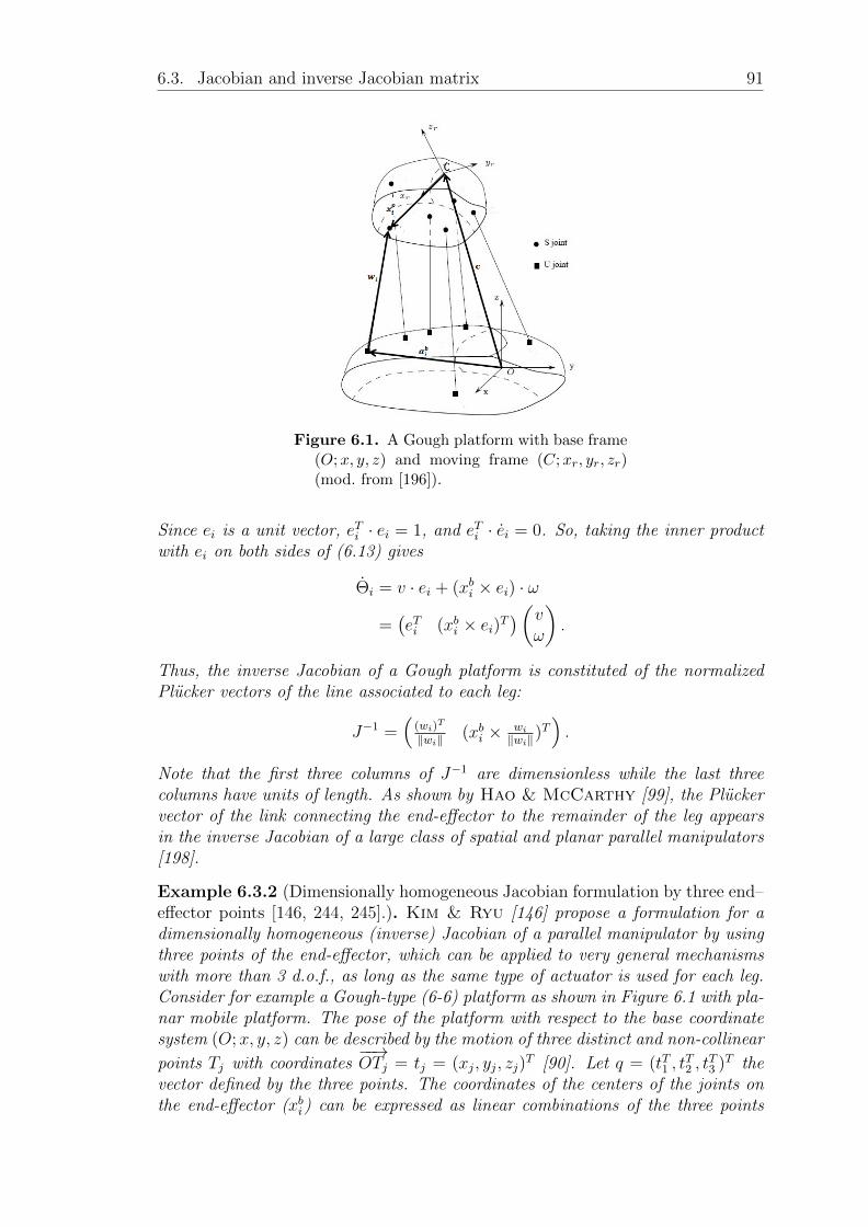
6.3. Jacobian and inverse Jacobian matrix 91
Figure 6.1. A Gough platform with base frame(O;x, y, z) and moving frame (C;xr, yr, zr)(mod. from [196]).
Since ei is a unit vector, eTi · ei = 1, and eTi · ei = 0. So, taking the inner productwith ei on both sides of (6.13) gives
Θi = v · ei + (xbi × ei) · ω
=(eTi (xbi × ei)T
)(vω
).
Thus, the inverse Jacobian of a Gough platform is constituted of the normalizedPlucker vectors of the line associated to each leg:
J−1 =(
(wi)T
‖wi‖ (xbi × wi
‖wi‖)T).
Note that the first three columns of J−1 are dimensionless while the last threecolumns have units of length. As shown by Hao & McCarthy [99], the Pluckervector of the link connecting the end-effector to the remainder of the leg appearsin the inverse Jacobian of a large class of spatial and planar parallel manipulators[198].
Example 6.3.2 (Dimensionally homogeneous Jacobian formulation by three end–effector points [146, 244, 245].). Kim & Ryu [146] propose a formulation for adimensionally homogeneous (inverse) Jacobian of a parallel manipulator by usingthree points of the end-effector, which can be applied to very general mechanismswith more than 3 d.o.f., as long as the same type of actuator is used for each leg.Consider for example a Gough-type (6-6) platform as shown in Figure 6.1 with pla-nar mobile platform. The pose of the platform with respect to the base coordinatesystem (O;x, y, z) can be described by the motion of three distinct and non-collinear
points Tj with coordinates−−→OTj = tj = (xj, yj, zj)
T [90]. Let q = (tT1 , tT2 , t
T3 )T the
vector defined by the three points. The coordinates of the centers of the joints onthe end-effector (xbi) can be expressed as linear combinations of the three points

92 Chapter 6. Differential kinematics
as xbi =∑3
j=1 kijtj with∑3
j=1 kij = 1 for dimensionless constants kij. Now, thevector wi describing leg i is given by
wi = (li + Θi)ei =3∑j=1
kijtj − abi , (6.14)
where li, Θi, ei and abi are described analogously to (6.12). Differentiating eq.(6.14) and multiplying with eTi yields
Θi =3∑j=1
kijeTi tj,
which can be represented in matrix form as
Θ = Nq, (6.15)
where N = J−1 is a dimensionless 6 × 9 matrix with J−1ij = (kije
Ti ), and q =
(t1T, t2
T, t3
T)T is the vector of generalized end-effector velocities. Note, that this
inverse Jacobian is an actual Jacobian as it is a matrix of partial derivatives ofCartesian coordinates with respect to the joint variables.
For other parallel mechanisms with n d.o.f. (n ≤ 6), a similar procedure can beapplied, which leads to a general (n × 9) inverse Jacobian J−1 = M−1N , whereM is a diagonal matrix and N is a matrix of the form as in (6.15). However,since for an n d.o.f. manipulator (n ≤ 6) at most only n terms are independentand so dependent motions are included, the physical significance of the singularvalues (which are relevant for dexterity analysis, see Ch. 7) of such a Jacobian isnot evident [146]. Pond & Carretero [244] further the proposed approach andobtain an m × n dimensionally homogeneous Jacobian, mapping the m actuatorvelocities Θi to n independent end-effector velocities. If the number of actuatorsequals the desired degrees of mobility, i.e., m = n (as in most cases), the pro-posed inverse Jacobian matrix is square. The inverse Jacobian proposed in [244]is derived as J−1 = J ′P where J ′ is the m × 9 inverse Jacobian of [146] and P a9× n constraining matrix, which is derived from differentiating relations betweenn selected independent terms and the dependent terms of the end-effector withrespect to the independent terms. This matrix relates the actuator velocities tothe n × 1 vector of independent end-effector velocities. This formulation of theJacobian may be used reliably for calculating dextrous regions of the workspace,or several dexterity indices as the condition number or singular values (see Ch. 7[244, 245].
Altuzarra et al. [3] develop a method for deriving a point-based, dimensionless,and comprehensive inverse Jacobian by presenting a novel numerical formulationof the velocity equation, which is to be compiled by general-purpose software andincludes all kinematic variables of the mechanism. The method uses a set ofkinematic restrictions applied to characteristic points of the mechanism and canbe applied to spatial mechanisms of any topology. Recently, Huang et al. [114]
6.3. Jacobian and inverse Jacobian matrix 93
proposed a “generalized Jacobian”, which makes it possible to integrate velocity,accuracy, and stiffness modeling of lower mobility serial and parallel manipula-tors with n ≤ 6 d.o.f. into a unified mathematical framework. The method usesscrew theory and the orthogonal and dual properties of wrench/twist subspacesand is used for a standardized and computational effective method for deriving adimensionally homogeneous n× n Jacobian of parallel manipulators [170].
6.3.2 Tasks
In analogy to the FKP and IKP, the forward instantaneous kinematic prob-lem (FIKP) is defined as determining the twist (and the passive joint velocities)as functions of the active joint velocities; the inverse instantaneous kinematicproblem (IIKP) then is to determine the active (and passive) joint velocities asfunctions of the twist. As the twist depends on the choice of the operating point,any relation involved in FIKP and IIKP will as well be affected by the location ofthis point [198]. As the inverse Jacobian (6.11) may usually be determined analyt-ically, the actuated joint velocities can be computed directly. For calculating thetwist, one can use for example a numerical inversion algorithm or a linear equa-tions solver to get the twist from (6.11); another method is to use a quasi-NewtonScheme (
vk+1
ωk+1
)=
(vkωk
)+ J0
(Θ− J−1
(vkωk
)), (6.16)
where J0 is the kinematic Jacobian calculated for a given pose [198].
The FIKP was solved, e.g., by Shi & Fenton [278], based on the velocities onthree non-collinear points of the end-effector. More recently, Lu & Hu [173]presented a uni- and simplified approach for the forward/inverse velocity and ac-celeration analysis of (limited) n d.o.f. parallel manipulators with linear actuators.
If the whole workspace is considered to find the worst case bounds on eithergeneralized velocity or joint rates, the FIKP and IIKP can be formulated as globaloptimization problems as ([219])
FIKPglobal: Given bounds on the joint rates, find worst case bounds on the gen-eralized velocity over a given type of workspace.
IIKPglobal: Given bounds on the generalized velocity, find worst case bounds onthe joint rates over a given type of workspace.
The solution of FIKPglobal provides the range of velocities that the robot can reach,while the solution of IIKPglobal allows the determination of the needed actuatorsfor performing the task in the designing process [219]. The FIKP is also importantfor robot position control and trajectory generation.
Huynh & Arai [125] analyze the maximum velocity of a general 6 d.o.f. manip-ulator in operational space using a (graphical) method based on the intersection
94 Chapter 6. Differential kinematics
of hyperplanes which are defined by the algebraic inequalities describing the con-straints on the kinematic model, and assuming that all articular velocities arebounded by the same limit, i.e., |Θi| ≤ ρ for all i ∈ 1, . . . , 6.
In the late 1990s, Merlet presented several algorithms which deal with certainproblems related to the FIKP and IIKP (see also [198, Ch. 5]). In [189] he describedan algorithm, which finds all possible parallel geometries such that the end-effectormay perform a given translational velocity for any location of the end-effector ina given workspace, with the constraint that the actuator velocities are alwayslower than given bound. Another algorithm for efficiently computing the articularvelocities necessary to perform a given translation/orientation velocity of the end-effector in the translational workspace is presented in [190]; and furthermore, in[192] Merlet proposes an efficient algorithm, which takes as assumption thatthe orientation of a parallel manipulator is constant over a given volume. It thencomputes, with a guaranteed error, the maximal and minimal articular velocitiesso that whatever the location of the end-effector is in the volume, it may performa motion in a given Cartesian/angular velocity. The proposed algorithm is muchfaster and safer than the classical discretization method [192]. However, solvingthe general case is still an open problem [198]. More recently, an interval analysis-based algorithm was presented in [203], which allows the calculation of the maximaland minimal full independent velocity XM
i and Xmi with
Xi :=n∑j=1
|Jij|
for all poses over an (almost) arbitrary workspace up to a given accuracy. How-ever, the algorithm is computer-intensive and an efficient calculation of Xm
i , XMi
is still an open problem [198]. In a comparative study of two 3 d.o.f. parallelmanipulators done by Chablat et al. [52], a method is described which allowsto prove formally whether the velocity amplification factors in a subpart of of theCartesian workspace remain within a predefined range or not.
6.4 Acceleration
To obtain similar relations for the joint and platform accelerations, the obtainedequations from the velocity-analysis must be again differentiated. The accelerationof point xb is given by differentiating (6.8) with respect to time to get
xb = ω × xb + ω × xb + a,
where
a :=Dv
Dt= c− ω × c− ω × c
is the platform acceleration and ω denotes the angular acceleration and isthe axial vector of the angular acceleration matrix Λ = Ω + Ω2, i.e.,
Ωx = ω × x.
6.4. Acceleration 95
Differentiation of (6.10) yields relations between the joint acceleration Θ and
the generalized acceleration or twist rate
(aω
). In particular, for parallel
manipulators the relation
Θ = J−1
(aω
)+ ˙J−1
(vω
)(6.17)
may be obtained directly by differentiating (6.11). In [6] and [198] a few examplesfor the acceleration analysis of serial and parallel manipulators, respectively, aregiven.
Example 6.4.1 (Acceleration analysis of a Gough platform). In Example 6.3.1,the joint rates Θ of a Gough platform are given by
Θ =(eTi (xbi × ei)T
)(vω
).
Thus, the joint acceleration Θ given by (6.17) are
Θi =(eTi uTi
)(vω
)+(eTi (xbi × ei)T
)(aω
),
where ui = xbi × ei + xbi × ei.
For the generalized acceleration, similar tasks as for the generalized velocity canbe posed [219].

96 Chapter 6. Differential kinematics

Chapter 7
Dexterity and Error Bounds
7.1 Introduction
The term dexterity1 refers to the ability of the manipulator to arbitrarily changeits position and orientation, or apply forces and torques in arbitrary directions[287]. In other words, dexterity summarizes the flexibility and accuracy withwhich the end-effector is placed in a given pose. The flexibility is quantified bythe dexterous workspace (see Section 4.4). The positioning accuracy of a manipu-lator depends on various factors, as sensor errors, manufacturing errors or thermalerrors. A short summary of several results concerning geometrical and thermalerrors may be found in [196, 198]; most recently, a review of error sources and er-ror compensation methods for serial and parallel manipulators was given by [181].Usually, joint sensor errors are the largest source of error [196]. To quantify theaccuracy, dexterity indices may be defined in numerous ways. These are widelyused for the design of manipulators (e.g., [88, 90, 143, 205, 268]), but there aresome concerns about the reliability of certain indices [197], due to the impossibilityto define a single invariant metric for the special Euclidean group [268] (see Section7.3 below). In this chapter, the modeling of the accuracy of a pose is discussedas well as several ways of measuring dexterity and tasks concerning accuracy anderror bounds.
The joint configuration Θ is given by more or less accurate measurements y ≈ PΘ.Since it is based on these measurements, the pose of the robot, as estimated bythe forward kinematics, is inaccurate. Thus, the manipulator accuracy ∆s (orthe error on the positioning of the robot) is induced by errors ∆Θ on the sensormeasurements (and joint sensor errors are usually the largest source of positioningerrors [196]). These errors are approximately (in first order) linearly related by arelation of the form
A(s,Θ)∆Θ = B(s,Θ)∆s, (7.1)
1Note, that in several publications the term dexterity is synonymously used for the relativeerror amplification described by the condition number of the Jacobian.
97

98 Chapter 7. Dexterity and Error Bounds
with A,B matrices depending on the state of the robot. For a serial manipulator(7.1) has the form
∆s = J(s,Θ)∆Θ, (7.2)
where J denotes the state-dependent kinematic Jacobian of the robot; for a Goughplatform (7.1) is given by
∆Θ = J−1(s,Θ)∆s, (7.3)
where J−1 is the pose-dependent inverse Jacobian matrix of the robot. The deter-mination of the (inverse) Jacobian is addressed in Section 6.3.
7.2 Modelling the accuracy of a pose
The pose of a robot depends on the chosen coordinate system for base and platformand the representation chosen for the rotation. Thus, the way of modelling theaccuracy of a pose shall be discussed more detailed. The geometric pose erroris given by
∆s =
(∆r∆c
); (7.4)
any single or aggregated error measure can be expressed as a function ε(∆s), de-pending on (7.4). The geometric pose errors may be expressed in terms of the errorcharacteristics of the measurements. In robotics, a commonly used representationof sensor accuracies is by worst case error bounds. Therefore, the measurementequation (4.2) is replaced by an inclusion
y = P∆Θ + ∆y, ∆y ∈ d, (7.5)
where d = [−d, d] is a tiny box consisting of all measurement errors ∆y with|yi| ≤ di for all i. The equation of state F (s,Θ) = 0 is satisfied by the true pose s
and joint configuration Θ. But the measured joint configuration Θ and the pose s,which is calculated by direct kinematics from the measured data, satisfy instead
F (s, Θ) = 0, P Θ = y,
which can be written in linearized form as
0 = F (s, Θ)
≈ F (s,Θ) + Fs(s,Θ)(s− s) + FΘ(s,Θ)(Θ−Θ), (7.6)
where Fs(s,Θ) and FΘ(s,Θ) denote the matrices of partial derivatives with respectto s and Θ, respectively. The pose s derived from inaccurate sensor measurementsconsists of a displacement part c and an orientation part r. These may be ex-pressed in the chosen parameterization for the rotation. In the following, a fewdetails of modelling pose errors using the quaternion parameterization shall begiven (for details see [219]). Note that similar formulas can be derived for otherrepresentations.
7.2. Modelling the accuracy of a pose 99
Let Q[r] be the rotation of the platform as described in Section 4.3 and Q[r] therotation derived from inexact sensor readings with r close to but different from r.The multiplication of Q[r]T and Q[r] again gives a rotation, which has the formQ[∆r] for some vector ∆r. To derive a formula for r, the equation
Q[r]TQ[r] = Q[∆r]
is multiplied by Q[r], which results in
Q[r] = Q[r]Q[∆r]. (7.7)
Using the product formula (4.12) and (7.7), orientation errors can be representedby
r = r ⊕∆r. (7.8)
Thus, it can be seen from the nonstandard addition formula, that rotations inthree dimensions usually do not commute (unlike in two dimensions, where anglessimply add). The displacement error ∆c can be written as
∆c = Q[r]T (c− c).
Multiplying again by Q[r], c can be expressed in terms of c and ∆c as
c = c+Q[r]∆c. (7.9)
For the analysis of small errors only, higher order terms may be dropped and (7.8)and (7.9) may be written in linearized form as
r ≈ r + e−12 (r0∆r + r ×∆r)
c ≈ c+Q[r]∆c. (7.10)
(7.10) may then be written in the form
s ≈ s+ E(s)∆s, E(s) =
(E[r] 0
0 Q[r]
), (7.11)
where
E[r] =1√e
r0 −r3 r2
r3 r0 −r1
−r2 r1 r0
.
Using (7.11) and Θ = Θ + ∆Θ, (7.6) can be written as
Fs(s,Θ)E(s)∆s+ FΘ(s,Θ)∆Θ ≈ 0.
Note that P∆Θ = P Θ − PΘ = ∆y ∈ d. Thus, the errors satisfy (in the linearapproximation) the constraints
DF (s,Θ)∆s+ FΘ(s,Θ)∆Θ ≈ 0, P∆Θ ∈ d, (7.12)
whereDF (s,Θ) = Fs(s,Θ)E(s). (7.13)

100 Chapter 7. Dexterity and Error Bounds
Equation (7.12) is the basic (linearized) formula for the quaternion representationrelating known measurement errors ∆Θ to pose errors ∆s. It also holds in otherrepresentations, if the expressions in (7.11) are replaced by the correspondingexpressions for the chosen representation. As an artifact of the normalizationused for the quaternion representation, equation (7.12) is ill-defined at r0 = 0and numerically unstable at small values of r0: on the one hand, due to thesquare root in the computation of r0 the quaternion representation has a gradientsingularity at r0 = 0; on the other hand, the matrix E(s) is singular at r0 = 0,since detE(s) = detE[r] = r0(
∑3i=0 r
2i ) = r0e. This problem can be solved by
treating r0 as an additional parameter constrained by r20 + r2 = e. By writing
r = r + ∆r, it follows from equation (7.10) that
r20 = e− r2
≈ e− r2 − 2e−12 r0r ·∆r
= r20 − 2e−
12 r0r ·∆r
≈ (r0 − e−12 r ·∆r)2,
so,r0 ≈ r0 − e−
12 r ·∆r. (7.14)
Equation (7.14) now can be written in the form
r0 ≈ r0 − E0(s)T ·∆s, E0(s) =
(e−
12 r
0
).
Concluding, by writing the equation of state (4.1) more carefully as
F (r0, s,Θ) = 0,
the constraints (7.12) are obtained by replacing (7.13) with the numerically stableexpression
DF (s,Θ) = Fs(r0, s,Θ)− Fr0(r0, s,Θ)E0(s)T .
Again, these formulas also hold for other representations, if the expression forE0(s) is replaced by corresponding expression for these representations [219].
7.3 Dexterity indices
As mentioned before, for applications several performance indices may be com-puted to measure the dexterity of a manipulator. Most discussed are “classical”dexterity indices: the condition number (of the Jacobian) [271] and the so-calledmanipulability index [338]. Due to their suffering from certain drawbacks andmissing reliability for parallel robots in particular [197] (see below), other waysfor measuring the accuracy are searched. It was shown that, especially for paral-lel manipulators, extremal positioning errors are more reliable than the conditionnumber; however, to compare two different designs in terms of accuracy, mean

7.3. Dexterity indices 101
value and variance will also be needed [196]. Just recently, kinematic sensitivityindices for rotation and translational displacement [39] or the power manipulability[177] have been introduced.
The dexterity indices discussed in the following sections evaluate (in a more or lessreliable way) the sensitivity of a robots performance to variations in its actuatedjoints, but they are not suitable for other types of uncertainties, such as variationsin geometric parameters. Thus, appropriate sensitivity measures were proposedby Caro et al. [40, 41] to evaluate the sensitivity of the pose of the end-effectorof a Orthoglide 3-axis manipulator to variations in its design parameters and tocompare planar parallel manipulators of the same architecture (3-RPR). Recently,Binaud et al. [17] introduced a methodology for 3 d.o.f. planar parallel manipu-lators to obtain the sensitivity coefficients of the pose of the moving platform tovariations in their geometric parameters and actuated variables to compare ma-nipulators of different architecture. Additionally, two aggregate sensitivity indiceshave been determined, one related to the orientation and the other one to the po-sition of the moving platform. The described method is able to take the sensitivityto joint clearances and flexibility in the revolute joints into account [17].
7.3.1 Error bounds depending on the norm
In practice, it is assumed that the measurement errors are bounded, which con-sequently poses a bound on the positioning errors. Without loss of generality,usually a boundary value of 1 is chosen, so
‖∆Θ‖ ≤ 1, (7.15)
which yields∆sTJ−TJ−1∆s ≤ 1. (7.16)
The geometrical interpretation of (7.16) differs depending on the choice of thenorm (see Figure 7.1 for the 2D case). By choosing the Euclidean norm, (7.15)represents a hyper-sphere in the joint error space which is mapped into the so-calledmanipulability ellipsoid. If the infinity norm is chosen, the absolute values ofthe joint errors are independently bounded by one and thus are restricted to lie in ahyper-cube within the joint error space, which is mapped into a convex polyhedron,the so-called kinematic polyhedron [197]. As Merlet pointed out, the infinitynorm provides a more appropriate and realistic mapping due to the independencyof the joint error bounds and additionally, computations involving a polyhedroncan be done more easily than involving ellipsoids [197, 198].
The two indices described in the following paragraphs are used for both serial andparallel manipulators. For simplification of the notation, their definition will beintroduced using the Jacobian J only.

102 Chapter 7. Dexterity and Error Bounds
Figure 7.1. The mapping between the joint errorspace and the generalized coordinates error spaceinduced by J−TJ−1 according to the Euclideannorm (on top) and the infinity norm (on bottom)for the 2D case [197].
7.3.2 The manipulability index
Manipulability is defined asµ =√
det JTJ
for a square, non-singular matrix J by Yoshikawa [338] for serial manipulatorsand has been adopted as a dexterity measure for parallel robots as well. It is alocal performance measure, since the Jacobian is pose dependent. Geometrically,the manipulability is (up to a proportionality constant) the volume of the ellipsoiddescribed above. The only use of the manipulability as dexterity index may causeproblems in automatic synthesis, as it may lead to manipulators with distortedgeometries [39]. Further, a limitation of this index may be that it is independentfrom the position of the operating point on the end-effector, and thus cannotdistinguish between a large and a small end-effector [39, 143]. Nevertheless, it isused for the dexterity analysis of several manipulators, e.g., in [166] for a 3-PRSparallel manipulator.
7.3.3 The condition number as error amplification factor
The error amplification factor in a system (7.3), or (7.2), expresses how a relativeerror in the joint coordinates Θ gets multiplied and yields a relative error in thepose s [197]. Salisbury & Craig [271] proposed the condition number
κ = ‖J‖‖J−1‖,
as a local performance index, where J−1 denotes either the inverse of the Jacobianor a pseudo-inverse (e.g., Moore-Penrose generalized inverse) [39]. The conditionnumber gives an upper and a lower bound for the relative error amplification ([39]),
1
κ
‖∆Θ‖‖Θ‖
≤ ‖∆s‖‖s‖
≤ κ‖∆Θ‖‖Θ‖
.
7.3. Dexterity indices 103
Thus, a minimization of κ should minimize the maximum relative error ampli-fication, but as a decreasing κ increases the lower bound on ‖∆s‖/‖s‖, it doesnot provide the overall relative error amplification. The condition number is de-pendent on the choice of the matrix norm; the most used norms are the 2-normand the Frobenius-norm [197]. In the former case, the condition number of theJacobian is given by
κ(J) =σmaxσmin
=
√λmaxλmin
,
where σmax, σmin denote the largest and smallest singular value of J , respectively,and λmax, λmin the largest and smallest eigenvalue of JTJ , respectively. If theFrobenius-norm is used, the condition number is given by
κ(J) =
∑λ2i∏λ2i
,
where λi are the eigenvalues of JTJ [197].
Merlet [197] critically evaluated the efficiency of the condition number for ac-curacy evaluation for a Gough platform. He concluded for various choices of thematrix-norm, that none of the tested condition numbers exhibits a completely co-herent behavior with respect to the accuracy of the robot. Thus, the use of thecondition number must be carefully considered. However, it is used in various pub-lications for describing the dexterity and/or optimizing the design of a robot (see,e.g., [172, 245, 246]). For serial manipulators, Kucuk & Bingul [151] proposed acombined performance index, which is a combination of the manipulability indexand the condition number; it is used for workspace optimization via sequentialquadratic programming for spherical 3-link manipulators.
A pose of a robot with κ = 1 is defined as isotropic pose, and a robot which hasonly isotropic poses is called an isotropic robot [197, 198]. Designing a parallelmanipulator that is isotropic in a pose or over its full workspace is often consideredas a design objective [73, 144, 297, 341].
7.3.4 Sensitivity indices
As discussed by several authors (e.g., [69, 169]), the described indices do not applyto Jacobians involving both translational and rotational velocities. Thus, severalattempts have been made to formulate a dimensionally homogeneous Jacobianby using either multiple end-effector velocities [3, 90, 114, 146, 170, 244–246], ora normalization procedure of different kinds [143, 168, 338]. However, Cardouet al. [39] pointed out, that both approaches require some kind of arbitrarinessor uncertainty (e.g., in choosing points or weighting factors), which in particularmakes any comparison between different robotic manipulators difficult. Thus,the authors recently proposed two distinct indices for the rotation and the point-displacement sensitivity. The considered problem is stated as finding the actuatordisplacements ∆s that generate actuator displacements of a fixed magnitude ‖Θ‖q,

104 Chapter 7. Dexterity and Error Bounds
while yielding global extrema of ‖∆r‖ and ‖∆p‖ [39]. The maximum solutions ofthis problem ,
σr,q := max‖Θ‖q‖∆r‖q, (7.17)
σp,q := max‖Θ‖q‖∆c‖q, (7.18)
give tight upper bounds on the amplitudes of rotations and operating-point dis-placements, and are defined as the maximum rotation sensitivity and point-displacement sensitivity, respectively. If for example q = ∞, i.e., the infinity-norm is chosen in (7.17) and (7.18), the sensitivity-indices for a parallel manipu-lator may be found by solving the optimization problem
max∆s
‖∆ ? ‖∞ (7.19)
s. t. ‖Θ‖∞ = ‖J−1∆s‖∞ = 1,
where ? = r or ? = p, respectively, and under the assumption that all actuatedjoint assemblies are the same. Geometrically, the constraint forms the envelope ofa polytope
P6(J−1) := x ∈ R6|‖J−1x‖∞ = 1.
Finding the supporting hyperplanes of a polytope may be cast into a linear pro-gram. Hence, as the objective function varies only along three independent direc-tions, computing the solution of (7.19) amounts to finding the solution of threelinear programs each, and choosing the maximal objective-function value amongthem [39].
The proposed sensitivity indices are “nothing but another method” [39], but havesome characteristics not present in other indices. So they have a clear and definitephysical meaning, rely on the Jacobian only, are unit-consistent, depend on thechoice of the operating point (contrary to the manipulability), and apply to anyuniformly actuated manipulator, regardless if redundantly actuated or not [39].Saadatzi et al. [268] use these sensitivity indices for the optimization of 3-RPRplanar parallel mechanisms.
7.3.5 Global dexterity
If the dexterity of a robot over a given workspace W shall be evaluated, generallya global conditioning index (GCI) is used as proposed by Gosselin [88]:
GCI =
∫W
1κ
dW∫W dW
,
where κ denotes the condition number (see also Gosselin & Angeles [92]). TheGCI can be used for the optimal design of a robot [172], but a main problem is
7.4. Errors and Global Optimization 105
its calculation. Usually, the workspace is sampled using a regular grid, 1/κi iscomputed at each node Ni, and the GCI is approximated by
GCIapprox =
∑ni=1
1κi
n.
The computational effort increases exponentially with respect to the number ofd.o.f. of the robot and additionally, this method does not provide a bound on|GCI−GCIapprox | [197]. Another evaluation method of the GCI may be using(quasi) Monte-Carlo integration. But a certified evaluation of the GCI is an openproblem and will probably be computer intensive [197].
7.4 Errors and Global Optimization
As mentioned, most dexterity indices are not very adequate for parallel manipula-tors [196], or provide at least not a precise knowledge of the extremal pose errors[30]. A better way is the determination of the maximal positioning (and orienta-tion) errors over a prescribed workspace (and further its mean value and variance[196]), or at a given configuration with known joint-sensor errors [30, 196]. Severaltasks concerning the maximal pose error and the accuracy of a robot can now beformulated [219]:
• Find the maximal pose error over a specified workspace given bounds (7.5)on the sensor accuracy for one ore more error measures ε(∆s).
• Find the sensor accuracy needed, to guarantee a specified maximal pose errorover a given workspace.
• Find the state (s,Θ) with the smallest maximal pose error.
• Find the set of states in which ∆s lies within a specified region.
• Find the average value (and the variance) of the maximal pose error overthe workspace, given a probability measure on the workspace (e.g. uniform).
The resulting optimization problems shall be discussed more detailed, following[219]. Consider the restricted case that all joint variables are measured, i.e., P = 1
and dimF ≥ dim s = 6. In the generic case, i.e., if rankDF (s,Θ) = 6, (7.12) canbe solved for ∆s:
∆s ≈ −DF (s,Θ)+FΘ(s,Θ)∆Θ, (7.20)
where DF+ denotes a pseudo-inverse of DF . So, in a fixed state, the geomet-ric pose errors are proportional to the measurement errors. However, since apseudo-inverse is expensive to compute, it is preferable to solve instead of (7.20)

106 Chapter 7. Dexterity and Error Bounds
an optimization problem for one or more error measures ε(∆s). For a robot in afixed state these are given by
max ε(∆s)
s. t. DF (s,Θ)∆s+ FΘ(s,Θ)∆Θ ≈ 0, (7.21)
∆Θ ∈ d,
or, if nonlinear corrections are significant,
max ε(∆s)
s. t. F (s,Θ + ∆Θ)− F (s,Θ) = 0 (7.22)
s =
(r ⊕∆r
c+Q[r]∆c
).
Both (7.21) and (7.22) are global optimization problems, since worst case errors arerequired. If the worst case accuracy over some workspace shall be computed, theformulations of (7.21) and (7.22) still hold; the constraints defining the workspacehave to be added and s and Θ have to be treated as additional variables. However,the size of the search space is much bigger, so the difficulty increases [219].
Kim & Choi [145] provided methods for the forward and inverse error boundanalyses (FEBA and IEBA)of the Stewart platform. Given the error bounds of thejoints, the FEBA is used to find the error-bound on the position of the platform.The IEBA, on the other hand, determines the error bounds on the joints for agiven error bound on the end-effector pose. The latter provides a designer witha way to calculate tolerance limits of the joints and is therefore important. Kim& Choi derived two eigenvalue problems corresponding to the FEBA and IEBA,where the eigenvalues from both analyses are reciprocal to each other.
Wang & Ehmann [317] present an error analysis for the Stewart platform, tak-ing location errors and imperfect motion in the ball-joints as well as errors in theactuated joints, i.e., in the leg lengths, into account. They propose a first and sec-ond error model and provide a software package (written in Mathematica) whichallows, for a given orientation of the platform, the determination of the workspaceregions where the positioning error is larger than a given threshold. Jelenkovic& Budin [131] present an online error analysis tool2 based on on the model pre-sented by Patel & Ehmann [232], which computes the worst case accuracy for6-UPS and 6-PUS hexapods. Pott & Hiller [248] give an approach to estimatethe first-order influence of geometric errors on target quantities by considering theforce transmission of the manipulator.
As pointed out by Merlet & Daney [203], several authors treated the problemof finding positioning errors of a given robot at some specific location within theworkspace (e.g., [145]; for further references see [203, p. 942]). Thus, in [203] notonly specific poses are considered but the whole workspace and further, the errorsynthesis problem is addressed, i.e., finding the geometries of a robot that have at
2available at http://hexapod.zemris.fer.hr/engleski/Online_en.htm)

7.4. Errors and Global Optimization 107
least a required accuracy [203]. As a by-product variant of the interval analysis-based algorithm it is possible to compute the maximal positioning errors of a given(6 d.o.f.) robot in a specified workspace up to a predefined accuracy. However, thealgorithm has a large computation time. Merlet [196] addresses a verificationproblem. Given the geometry of a robot (possibly with uncertainties), bounds onthe sensor errors, and a prescribed workspace, the proposed algorithm checks if themaximum of the positioning errors does not exceed some threshold. As a result, theworkspace is identified as safe, if for any pose within the workspace the positioningerror will be lower than the threshold, or unsafe, if there is at least one pose with apositioning error exceeding the threshold (or, in some cases, the algorithm is unableto decide). Here, the main objective is not to calculate maximal positioning errorsper se but to verify that they stay below some threshold. However, this method isrelatively difficult to implement and gives no information on the evolution of theaccuracy of the manipulator within the workspace [29]. Moreover, Merlet [196]points out, that in addition to the maximal pose errors it may be important tocompute their mean value and the variance; but it is a challenging task to definean algorithm to compute those, at least approximately with a guaranteed error.
A geometric approach is given in [30, 339] to compute the exact value of the poseerror of a 3 d.o.f. planar parallel manipulator at a given nominal position. Yu et al.[339] introduce the method for 3-PRP planar parallel manipulators, replacing theexisting dexterity maps by maximum position/orientation error maps. Briot &Bonev [30] generalize this work for all fully-parallel 3 d.o.f. planar parallel manip-ulators and prove that, when sufficiently far from singularities, the local maximumorientation/position errors can occur only when at least two active joint inputs suf-fer a maximal error. Wang et al. [314] recommend an exact error bound contrary
Figure 7.2. Comparison of the exact output errorXd to the maximal error Xmax evaluation: alongthe operating direction d with allowed maximaloutput error Xr, the accuracy performance satis-fies the required operating precision forXd(< Xr),but for Xmax(> Xr) not [314].

108 Chapter 7. Dexterity and Error Bounds
to a maximal error bound, which represents the extremal value of the maximaloutput errors in each direction, and thus may be limited to evaluate the accuracyperformance in some case (see Fig. 7.2). The forward error bound analysis for an nd.o.f. manipulator at a given nominal configuration s0 is stated as constraint opti-mization problem and then the exact output error bound, which can be indicatedby a closed curve or surface, is computed using the level set method by trackingthe propagation of the output error interface under the constraints of the activejoints’ input errors. The algorithm is quite easy to implement as it only requiresthe inverse kinematic functions of the manipulator. The proposed method notonly provides a prediction of the exact error bound but also the best/worst errortransformation direction and the output accuracy information along an arbitrarydirection. Thus, it has been proven, that a manipulator may admit completelydifferent accuracy properties along different directions. The method can also beapplied to compute the exact error bound over a given trajectory or part of theworkspace. For example, the exact error surface of a Delta parallel manipulatorwas computed, needing 15 iterations and about 226.5 seconds (see Fig. 7.3).
Figure 7.3. Propagation of the output error surface of theDelta manipulator for t = 1, 3, 8, 15 iterations [314]
A (so far) open problem is to locate a priori the poses with the worst positioningaccuracy [198]: according to Merlet [198] it was shown by Hay & Snyman [104]that for planar robots the worst values of the condition number are obtained forposes on the boundary of the workspace. However, this result relies on numericalcalculation and it is an open problem to determine if this is also true for spatialrobots, and for the worst positioning error as well.
Another aspect that has to be considered is the influence of joint clearance on theposition accuracy of robotic manipulators (see, e.g., [295]). Joint clearance, i.e., thedistance between the mating surfaces of a joint, leads to uncertain flawed motionsat an arbitrary pose of the mechanism and its effects are highly non-repeatable.For example, Meng et al. [183, 184] propose an efficient error evaluation methodfor parallel mechanisms which can be used to predict the global maximum pose
7.4. Errors and Global Optimization 109
errors of a clearance-affected mechanism in a prescribed workspace, by formu-lating the problem as a standard convex optimization problem. Chebbi et al.[54] develop an analytical predictive model for quantifying the pose error of a 3-UPU parallel manipulator as a function of the magnitude of the joint clearance,the external load acting on the platform, and the configuration of the manipu-lator. Furthermore, an algorithm is given which maps the pose error within theworkspace of the robot, and thus allows a determination of the distribution of theerror within the workspace, which may have a discontinuity due to the change ofthe configuration of the robot. More recently, Frisoli et al. [83] present a screwtheory based method which computes the worst position accuracy for spatial par-allel manipulators with revolute joint clearances and performs a maximization ofthe pose error function in a mixed analytical-numerical approach, converging tothe exact maximum pose error.
Finally, a noteworthy comparison between serial and parallel manipulators regard-ing the accuracy done by Briot et al. [29] shall be mentioned. It is often claimedthat parallel manipulators have a higher accuracy than serial ones (e.g., [54]) be-cause their errors are averaged instead of cumulatively added [29]. A comparisonof serial and parallel 2 d.o.f. manipulators seems to indicate that parallel mech-anisms are less sensitive to input errors, but the study is too limited to state ageneral assumption. Furthermore, the authors state that a meaningful comparisonbetween other pairs of serial and parallel mechanisms is virtually impossible.

110 Chapter 7. Dexterity and Error Bounds

Chapter 8
Singularities
8.1 Introduction
In this chapter, the notion of singularities1 shall be defined and described in moredetail. Singularities are particular poses of the end-effector in which either theforward or the inverse instantaneous kinematic problem becomes undeterminate,and thus, the properties of the mechanism change dramatically. In a singularconfiguration, the pose of the end-effector is no longer controllable, and forces,imposed on several links, may become very large, which may cause a breakdownof the robot. Therefore, singularity analysis is an important field of study inrobotics, it plays a significant role in the design and control of robot mechanisms.
8.2 Singular configurations
The relationship between input (joint variables) and output (end-effector position)coordinates of any manipulator is given by the equation of state (4.1)
F (s,Θ) = 0,
where s is a set of parameters coding the pose of the end-effector and Θ describesthe joint configuration (including active and passive joint parameters). It allowsto formulate a relation of the type (cf. (7.1))
A(s,Θ)∆Θ = B(s,Θ)∆s,
where ∆Θ denotes the error of the vector of joint positions, ∆s the error in thepose of the end-effector, and A = A(s,Θ) and B = B(s,Θ) are both configura-tion dependent n × n matrices (for a n d.o.f. non-redundant manipulator). Fora non-redundant parallel robot with n actuated joints (and n d.o.f.) for a total
1An extensive database of publications about singularities in robot kinematics can be foundat http://homepages.mcs.vuw.ac.nz/~donelan/cgi-bin/rs/main.
111

112 Chapter 8. Singularities
of N joints, the equation of state (4.1) consists of a set of N equations in N + nunknowns. A kinematic singularity exists if the rank of the kinematic Jacobianof the system is less than N, or equivalently, if there are less than N independentequations. Considering (7.1), that means that one of the matrices A or B be-comes singular, i.e., det(A) = 0 or det(B) = 0. Thus, in principle three types ofsingularities may be distinguished [91]:
(1) A is singular (called serial or type 1 singularity).
(2) B is singular (called parallel or type 2 singularity).
(3) A and B both are singular (called type 3 singularity).
In principle, at a serial singularity a robot loses degree(s) of freedom, while ata parallel singularity degree(s) of freedom are gained, i.e., the manipulator canmove while the actuators are locked. As for many serial manipulators B = 1,a singularity only happens if det(A) = 0. A parallel singularity lies within theworkspace and happens in particular for parallel manipulators.
The general description of singularities by Gosselin & Angeles [91] is basedon the input and output velocities. Park & Kim [231] applied methods fromdifferential geometry and introduced three basic singularity types. The singularity-taxonomy is independent of the local coordinates used to describe the kinematics,and includes mechanisms that have more actuators than d.o.f. A more generalclassification was proposed by Zlatanov et al. [348], where not only the inputand output velocities, but also the passive-joint velocities are included explicitly. Ageneral manipulator model, in terms of differentiable mappings between manifolds,allows a rigorous mathematical definition of kinematic singularity. Input, outputand configuration-space singularities are identified as the three basic types, butalso a finer classification using six types is given, depending on the cause of thedegeneracy.
There are different ways to introduce singular configurations, i.e. by studying therelation of input and output velocities, by studying the mechanical equilibrium orby studying the uniqueness of the solution to the FKP around a given solution[198]. In the following, we restrict our considerations to parallel manipulators; forresults about serial manipulators see, e.g., [140, 316].
8.2.1 Singularities and velocities
Differentiating the equation of state (4.1) with respect to time gives the relation
AΘ +Bw = 0 (8.1)
between the actuated joint velocities Θ and the twist w of the end-effector. A se-rial singularity means that a zero twist of the end-effector is obtained for non-zero
8.2. Singular configurations 113
actuated joint velocities. In that case the IIKP (cf. Chapter 6) is not solvable.For a robot having revolute joints between the attachment points of the legs itcan be shown that a pose on the boundary of the workspace causes a serial sin-gularity [198]. However, the converse is not true; a counter-example has beengiven by Bonev et al. [28]. A parallel singularity means that a non-zero twistw of the end-effector is obtained although the actuators are locked. Locally (inthe neighborhood of such a configuration), the end-effector is able to accomplishinfinitesimal motion. As in the case of locked actuators the mobility of the end-effector should be zero, it is said that the robot gains some d.o.f. Thus, certaindegrees of freedom of the robot cannot be controlled. In other words, kinematicsingularities are configurations in which there is a change in the expected or typ-ical number of instantaneous degrees of freedom [68]. A configuration is definedas non-singular when both the FIKP and the IIKP have unique solutions for anyinput or output [23].
8.2.2 Singularities and forces
A robot is in a mechanical equilibrium if the joint forces/torques τ balance thewrench F acting on the end-effector. The fundamental relation
τ = J(s)TF ,
where J(s) denotes the kinematic Jacobian, is valid for serial as well as parallelmanipulators. In a singular configuration the joint forces may go to infinity asthey are obtained by solving the linear system
F = J−T τ.
Hence, there is a significant risk of a breakdown of the robot (as reported in [198]).Therefore, it is important to be able to find such singularities.
8.2.3 Singularities and kinematics
For fixed actuated joint variables Θ the inverse kinematics equation of a robotmay be written as
F (s) = 0. (8.2)
Singularities may now be introduced by studying the uniqueness of solutions ofthe FKP around a given solution. If the Jacobian is non-singular, there is onlyone solution in a neighborhood while for a singular Jacobian multiple solutionsare obtained, i.e., the platform will be movable although the actuators are locked.Singularities are related to the study of kinematic branches. For a given setΘ1 of actuated joint variables, a finite set of solutions of (8.2) is derived. If theactuated joint variables Θ1 vary continuously to another set Θ2, then the solutionsof (8.2) also vary continuously: the poses of the end-effector follow different tra-jectories, the kinematic branches. A singularity occurs if two branches collapse,or if a branch goes to infinity [198].

114 Chapter 8. Singularities
8.3 Singularity Analysis
Singularity analysis is an important element in the process of designing and devel-oping a robot and has been intensively studied in the past two decades. As pointedout by Merlet [199] the search of singular configurations of parallel robots de-pends on the study of the singularities of the full (6×6) inverse kinematic JacobianJ−1(cf. Section 6.3), even for robots with less than 6 degrees of freedom. The fullinverse Jacobian is usually derived through a velocity analysis or through an anal-ysis of the mechanical equilibrium, as described above. The main problem is thatalthough an analytical form of J−1 may be known, the expansion of the deter-minant leads to huge expressions. A closed form for the determinant can usuallybe calculated for planar or spherical robots with 3 d.o.f. but will be more compli-cated for a larger number of d.o.f. [198]. A number of authors have sought to applymethods of mathematical singularity theory to the examination of singularities (asurvey can be found in [67]). Another approach (following [185]) uses Grassmanngeometry [198, 326] and Grassmann–Cayley algebra [4, 14, 15, 326] to determinesimpler singular conditions. But calculating the determinant is only the first stageof the singularity analysis; the second stage then is to find poses that cancel thedeterminant, which is an even more difficult task.
8.3.1 Determination of the singularity-free workspace
Ideally, the regularity of the inverse Jacobian should be checked for all poses ofthe useful workspace, i.e., the part of a robots workspace in which the end-effectorwill be most commonly located [199], or for any pose along a given trajectory.Furthermore, a suitable algorithm should be able to take uncertainties in therobot modeling and control into account and the singularity detection should becertified, i.e., the algorithm should provide safe answers even in the presence ofnumerical round-off errors. The singularity-detection problem has been addressedby Merlet [199], Merlet & Daney [202], where symbolic computation wasused to derive an analytical form of the determinant of J−1 and its sign at aparticular pose s0. Then, an interval analysis-based algorithm was applied, whichpermits to determine if the motion variety, i.e. a variety defined by the end-userwithin which the robot is constrained to move, includes a set of poses in whichthe determinant has a sign opposite to the one in s0. However, in particularif uncertainties (e.g., in the geometrical parameters of the robot) are added asadditional unknowns in the components of J−1, obtaining a closed-form of thedeterminant is no longer possible. Thus, a numerical method may be appliedto evaluate the determinant based on the interval form of the inverse Jacobian.However, such a numerical evaluation will lead to large overestimation of the truerange of the determinant and hence, to large computation times for the singularitydetection scheme. Therefore, it is necessary to develop methods that check theregularity of the set of matrices defined by an interval matrix without calculatingits determinant, and thereby take into account, that the inverse Jacobian is aparametric matrix, i.e., that its components are not independent. Merlet &

8.3. Singularity Analysis 115
Donelan [206] adress this problem and propose several methods to facilitate theregularity check. The algorithm given in [199] uses these methods and providesrobust in-workspace detection of singularities for any type of robot and with almostany type of motion variety in acceptable computation time; additionally it is ableto manage uncertainties in the control and the modeling of the robot.
For planar parallel manipulators Kotlarski et al. [149] present an improvedmethod to obtain the guaranteed singularity-free workspace. In order to avoidthe inconvenient interval form of the determinant of J−1 a geometrical-basedsolver is proposed. The method achieves significant improvements compared toa (preconditioned) interval evaluation of the det(J−1) in terms of the guaran-teed singularity-free zones in the workspace and the number of bisections used inthe branch-and-bound algorithm. However, the algorithm is restricted to specialmanipulator-geometries.
Recently, Bohigas et al. [23] presented a practical method to compute all types ofsingularities of non-redundant manipulators with no-helical lower pairs and desig-nated instantaneous input and output speeds. A system of quadratic polynomialequations for each singularity-type described by Zlatanov et al. [349] is definedthat encodes all singular configurations, and of which all solutions are initiallybounded in a box B. The algorithm for solving the system numerically recursivelyapplies a box shrinking and splitting procedure, where the box shrinking is basedon solving two linear programs. The method is applicable to manipulators witharbitrary geometry and will isolate singular configurations with a desired accuracy.In order to complete the task of exhaustive classification of the singularity set ofa given mechanism, Bohigas et al. [22] give an efficient method to compute sucha classification by means of a hierarchy of singularity tests.
It may be of interest to define a geometrical object such as a sphere or a cubeand determine the largest such object that is singularity free and enclosed entirelyin the workspace (see also Chapter 4.4). Algorithms to accomplish this task aregiven, e.g., by Li et al. [163] or Jiang & Gosselin [132].
8.3.2 Singularity index
Often one wants to define a “distance” to measure how “far” a given non-singularpose is from a singularity. The definition of such a distance in a mathematicalsense of a metric only is possible if the degrees of freedom are either translationalor rotational. In the presence of mixed d.o.f. only a weaker concept of singular-ity indices may be defined. Voglewede & Ebert-Uphoff [308] state a fewconditions a singularity index should fulfill and define various such indices in thevelocity domain as well as in the force domain. The generic form of a singularityindex in the velocity domain is formulated (using the joint velocities Θ and the

116 Chapter 8. Singularities
twist w) as constrained optimization problem
min ΘTUΘ
s. t. Θ = J−1w
wTVw = 1.
Various (somewhat arbitrary) choices of the matrices U, V are proposed suchthat ΘTUΘ and wTVw have a physical meaning. The calculation of the index isequivalent to solving a generalized eigenvalue problem. Liu et al. [171] proposeseveral indices to measure closeness to a singularity by taking motion/force trans-missibility into account. Hong [112] presents an index which provides a uniqueinvariant measure of closeness to a singular configuration for non-redundant serialand parallel manipulators, based on the screw-based Jacobian.
However, a major drawback of singularity indices is that they usually do not havea closed form. The indices may be computed numerically for a given robot andpose, but minimum, average value, and standard deviation over a given workspaceor trajectory are difficult to acertain (but may be important in practice) [198].
8.3.3 FKP and path planning
Singularities may also be useful in some cases, e.g., to sort the solutions of theFKP. As we have seen in Chapter 5, there are methods available to determine allsolutions of the problem, but the determination of the solution corresponding tothe current pose still poses a challenging problem. The workspace of the robotmay be separated into different regions that are singularity-free and separated bysingularity varieties. Wenger et al. [324] introduce these so-called aspects forparallel manipulators (see also [48, 325]). Usually a manipulator operates withinthe aspect which includes the initial assembly mode. Thus, a forward kinematicsolution will be a candidate to be the current pose only if it can be reached from aninitial assembly mode by a singularity-free trajectory. However, it is a non-trivialtask to determine the existence of such a trajectory. For a symmetrical planarparallel manipulator with equilateral base and platform triangle the existence ofsuch a non-singular assembly-mode changing trajectory was shown by Chablat& Wenger [49]. Husty [121] then proved for general planar 3-RPR parallelmanipulators the ability to pass from one solution of the FKP to another with-out crossing a singularity, and gave a technique how to construct singularity-freetrajectories that join all assembly modes of one connected component (see alsoChablat et al. [47]).
Just recently, Bohigas et al. [20] present a singularity-free path planning al-gorithm that attempts to connect two given non-singular configurations of anynon-redundant closed-chain manipulator. The method relies on defining a systemof equations whose solution manifold corresponds to the singularity-free subset ofthe configuration space. This manifold then is explored systematically by a higher-dimensional continuation strategy (as given in [130]), until a path joining the twoconfigurations is found (or the non-existence of such a path is determined).

Conclusion
The science of robotics is a field with high interdisciplinary character. It posesa large number of complex and challenging problems–interesting not only from amechanical but also from a mathematical point of view.
In the last two decades parallel manipulators have become more and more popular,especially for applications demanding high load carrying capacity or precise posi-tioning. Further advantages of parallel manipulators over their serial counterpartsfor certain applications are low inertia, higher structural stiffness, and reducedsensitivity to certain errors. Parallel robots are intrinsically more accurate thanserial robots as their errors are averaged instead of added cumulatively. How-ever, in terms of size of the (dexterous) workspace or with respect to the sufferingfrom singularities, the performance of parallel robots is poor compared to serialmanipulators.
The application area of parallel robots in particular is a broad field; for exam-ple, they are used for industrial tasks (e.g., tyre testing, Gough & Whitehall[94]), space applications (e.g., the Canterbury satellite tracker, Jones & Dunlop[137]), or in medical science, Sima’an et al. [281] (e.g., for prostheses with paralleltopology, Mendoza-Vazquez et al. [182], or a micro-manipulator for ophthalmicsurgery, Grace et al. [95]); see also, e.g., Patel et al. [233], Weck & Staimer[321]. Due to the higher level of complexity problems concerning parallel manip-ulators are more difficult to solve than problems for their serial counterparts. Inprinciple, the problems become more ambitious for an increasing number of degreesof freedom. Over the past years the number of publications has been growing forparallel manipulators. The benchmark for books concerning parallel manipulatorsis the one written by [198].
Since a various number of (parallel) architectures and geometries is possible withmostly quite distinct properties, each class of manipulators poses its own spe-cific problem formulations, and proposed solution methods and algorithms arerestricted to the special robot type. However, recent publications (e.g., Bohigaset al. [21, 22, 23], Cardou et al. [39], Liu et al. [170], Merlet [199], Petuyaet al. [239], Wang et al. [314]) aim to constitute unifying frameworks for severalproblems whose application spectra are as general as possible.
The problems surveyed in this thesis only cover a small amount of fundamentalquestions related to robotics. Further topics are concerned with, e.g., trajectory
117

118 Conclusion
planning, dynamical aspects, statics and forces, synthesis and design of robots.The distinct areas often heavily depend on each other, so it is usually quite difficultto treat one single problem without dealing with others at the same time. Theprobably most challenging problems are concerned with designing a robot thatprovides certain properties specified by the tasks it shall accomplish. During thedesign process from the initial stages of the conceptual definition of the robot tothe real prototype, most of the tasks presented in the previous chapters (and someadditional ones) have to be taken into account. Due to lack of writing space,the design-aspect was not discussed here. Hernandez et al. [106], Merlet &Daney [205] give a design methodology for parallel manipulators.
Considering the mathematical aspects in robotics, the highly interdisciplinarycharacter can be seen as well. The set of displacements which represent the mo-tion of rigid bodies, has the special structure of a group and is directly related tothe special Euclidean group SE(3), which is a differentiable manifold, a so-calledLie group. Thus, algebraic and differential geometry as well as the concept ofLie group theory plays an important role for the analysis and formulation of theproblems (see e.g., Selig [275]). Most of the problems arising in robotics heavilydepend on the solution of highly non-linear and often algebraic (systems of) equa-tions. Several solution methods, i.e., homotopy, elimination, Grobner bases, andinterval analysis, were outlined in previous chapters, and their main advantagesand disadvantages explained. In recent research certain algorithms have been de-veloped which improve the performance of Grobner basis- and homotopy-methodsin particular. Furthermore, interval analysis methods are getting more populardue to improved computer performance, which provides decreasing computationtimes. Due to the non-linearity, there are multiple solutions to the problems, andhence, methods for selecting the right solution have to be found. Up to now, thisproblem has not been solved in a satisfactory way, and hence, may be addressedin future work.
In many cases it is computational expensive or not possible to derive closed-formformulations of the equations. In either case, or, if uncertainties such as measure-ment errors or manufacturing tolerances have to be taken into account, numericalmethods are required. To derive certified and reliable results even in the presenceof uncertainties and round-off errors, methods of rigorous computing are needed,e.g., round-off error analysis (Wilkinson [327, 328]), interval arithmetical tools(Moore et al. [208], Neumaier [218]), or automatic differentiation (Bliek et al.[18], Bucker et al. [36], Schichl & Markot [273]). However, the aspect ofderiving rigorous solutions often is ignored, and thus, future work may addressthis problem.
For several applications, a worst-case analysis is required, and thus, global prob-lems have to be solved. Hence, (global) optimization problems need to be con-sidered. In the past few years, global optimization methods have been improvedquite significantly. However, to my best knowledge, up to now rigorous globaloptimization methods are used quite rarely in robotics. Therefore, this opens awide field for future research. For solving global optimization problems, various

Conclusion 119
relaxation methods, techniques for constraint propagation and higher order con-straint propagation, need to be utilized. In addition, inclusion/exclusion regionsare required for reducing the so-called cluster effect (Schichl et al. [274]) whichcauses big performance problems when solving systems of equations. For roboticsproblems it is a necessity to use various equivalent mathematical formulations ofthe same problem (Lie group, trigonometric functions, polynomial systems) sincesome solution techniques work better on some of the formulations than on others.It may be essentially important to improve the methods for rigorous computationin Lie groups, using a generalization of interval arithmetic to Lie groups.
From a personal point of view, robotics is a quite fascinating topic, in particu-lar because it interfaces multiple disciplines. Additionally, robotics is a field ofresearch which yields practical results that may have a positive impact and ben-efit on society. The work on this thesis was a challenging task for me. On theone hand, because I have no engineering background, and thus, it took quite awhile to understand and interrelate the research results; especially the apparentlycountless number of different manipulator types got confusing for me at times.Furthermore, due to different interpretations and varying use of the same termsand notation, it sometimes was a non-trivial task to draw contextual conclusions.On the other hand, the work on this thesis required the study and combination ofseveral mathematical methods, which I never have studied in detail up to now, oronly in a theoretical context. However, this thesis provides only a starting pointfor me and I intend to do further research in this area.

120 Conclusion

Appendix
121


List of Figures
3.1 Symbolic representation of revolute and prismatic joints [286, p. 13]. 42
3.2 The six lower kinematic pairs [57, p. 63]. . . . . . . . . . . . . . . . 43
3.3 6 degrees of freedom [http://www.dovermotion.com/images/knowledgecenter/accuracy1_large.gif]. . . . . . . . . . . . . . . . 44
3.4 A serial manipulator with 6 d.o.f. (T3) [152]. . . . . . . . . . . . . . 44
3.5 The original Gough platform (or octahedral hexapod) [24]. . . . . . 46
3.6 Coordinate frames of a Puma robot [6, p. 133]. . . . . . . . . . . . . 47
3.7 Denavit-Hartenberg parameters (mod. from [257]). . . . . . . . . . . 49
3.8 A 3R planar robot arm and its kinematic skeleton [313, p. 7]. . . . . 49
3.9 Screw displacement (mod. from [96]). . . . . . . . . . . . . . . . . . 52
3.10 A general 6R manipulator with decoupled architecture [6, p. 142] . 52
3.11 Scheme of a Gough platform (mod. from [196]). . . . . . . . . . . . 54
4.1 A Gough-Stewart platform of type MSSM (Maximal Simplified Sym-metric Manipulator) and its maximal singularity-free orientationworkspace [132]. . . . . . . . . . . . . . . . . . . . . . . . . . . . . . 68
5.1 A 3R planar robot arm and its kinematic skeleton [313, p. 7]. . . . . 70
5.2 Fundamental vectors for establishing the inverse kinematics of a6-UPS platform [198, p. 99]. . . . . . . . . . . . . . . . . . . . . . . 74
5.3 The 3-RRR type planar parallel manipulator [198, p. 98]. . . . . . . 75
5.4 A Griffis-Duffy platform [283]. . . . . . . . . . . . . . . . . . . . . . 79
6.1 A Gough platform (mod. from [196]) . . . . . . . . . . . . . . . . . 91
123
124 List of Figures
7.1 Mappings between the joint error space and the generalized coordi-nates space induced by J−TJ−1 [197]. . . . . . . . . . . . . . . . . . 102
7.2 Comparison of the exact output error Xd to the maximal error Xmax
evaluation [314]. . . . . . . . . . . . . . . . . . . . . . . . . . . . . . 107
7.3 Propagation of the output error surface of the Delta manipulator[314]. . . . . . . . . . . . . . . . . . . . . . . . . . . . . . . . . . . . 108

References
[1] M. Agheli and S.S. Nestinger. Closed-form solution for reachable workspaceof axially symmetric hexapod robots. In Mechatronics and Embedded Sys-tems and Applications (MESA), 2012 IEEE/ASME International Confer-ence on, pp. 75–80. IEEE, 2012.
[2] E.L. Allgower and K. Georg. Numerical path following. Handbook of Nu-merical Analysis, 5(3):207, 1997.
[3] O. Altuzarra, O. Salgado, V. Petuya, and A. Hernandez. Point-based Jaco-bian formulation for computational kinematics of manipulators. Mechanismand Machine Theory, 41(12):1407–1423, 2006.
[4] S. Amine, M. Tale Masouleh, S. Caro, P. Wenger, and C. Gosselin. Singular-ity analysis of 3T2R parallel mechanisms using Grassmann–Cayley algebraand Grassmann geometry. Mechanism and Machine Theory, 52:326–340,2012.
[5] J. Angeles. Is there a characteristic length of a rigid-body displacement?Mechanism and Machine Theory, 41(8):884–896, 2006.
[6] J. Angeles. Fundamentals of robotic mechanical systems. Springer, 3rd ed.,2007.
[7] J. Apel. A Grobner approach to involutive bases. Journal of SymbolicComputation, 19(5):441–457, 1995.
[8] L. Baron and J. Angeles. The direct kinematics of parallel manipulators un-der joint-sensor redundancy. Robotics and Automation, IEEE Transactionson, 16(1):12–19, 2000.
[9] L. Baron and J. Angles. The kinematic decoupling of parallel manipulatorsusing joint-sensor data. Robotics and Automation, IEEE Transactions on,16(6):644–651, 2000.
[10] A.H. Barr, B. Currin, S. Gabriel, and J.F. Hughes. Smooth interpolationof orientations with angular velocity constraints using quaternions. In ACMSIGGRAPH Computer Graphics, vol. 26, pp. 313–320. ACM, 1992.
[11] D.J. Bates, J.D. Hauenstein, and A.J. Sommese. Efficient path trackingmethods. Numerical Algorithms, 58(4):451–459, 2011.
125

126 References
[12] D.J. Bates, J.D. Hauenstein, A.J. Sommese, and C.W. Wampler. Bertini:Software for numerical algebraic geometry. Webpage, 2012. URL http:
//www.nd.edu/~sommese/bertini.
[13] C. Beltran and A. Leykin. Certified numerical homotopy tracking. Experi-mental Mathematics, 21(1):69–83, 2012.
[14] P. Ben-Horin and M. Shoham. Singularity analysis of a class of parallelrobots based on Grassmann–Cayley algebra. Mechanism and Machine The-ory, 41(8):958–970, 2006.
[15] P. Ben-Horin and M. Shoham. Application of Grassmann–Cayley Algebra toGeometrical Interpretation of Parallel Robot Singularities. The InternationalJournal of Robotics Research, 28(1):127–141, 2009.
[16] P.R. Bergamaschi, S. Saramago, and L.S. Coelho. Comparative study ofSQP and metaheuristics for robotic manipulator design. Applied numericalmathematics, 58(9):1396–1412, 2008.
[17] N. Binaud, S. Caro, and P. Wenger. Sensitivity comparison of planar parallelmanipulators. Mechanism and Machine Theory, 45(11):1477–1490, 2010.
[18] C. Bliek, C. Spellucci, L.N. Vicente, and A. et al. Neumaier. Algorithmsfor solving nonlinear constrained and optimization problems: The state ofthe art. Online, 2001. URL http://www.mat.univie.ac.at/~neum/glopt/
coconut/StArt.html.
[19] L. Blum, F. Cucker, M. Shub, and S. Smale. Complexity and real computa-tion. Foreword by Richard M. Karp. 1998.
[20] O. Bohigas, M.E. Henderson, L. Ros, and J.M. Porta. A singularity-free pathplanner for closed-chain manipulators. In Robotics and Automation (ICRA),2012 IEEE International Conference on, pp. 2128–2134. IEEE, 2012.
[21] O. Bohigas, L. Ros, and M. Manubens. A unified method for computingposition and orientation workspaces of general Stewart platforms. ASMEConference Proceedings, 2011(54839):959–968, 2011.
[22] O. Bohigas, D. Zlatanov, M. Manubens, and L. Ros. On the numericalclassification of the singularities of robot manipulators. In Proc. of the ASMEInternational Design Engineering Technical Conferences, 2012.
[23] O. Bohigas, D. Zlatanov, L. Ros, M. Manubens, and J.M. Porta. Numeri-cal computation of manipulator singularities. In Robotics and Automation(ICRA), 2012 IEEE International Conference on, pp. 1351–1358. IEEE,2012.
[24] I.A. Bonev. paralleMIC. Webpage, 2012. URL http://www.parallemic.org.
[25] I.A. Bonev and C.M. Gosselin. Analytical determination of the workspaceof symmetrical spherical parallel mechanisms. Robotics, IEEE Transactionson, 22(5):1011–1017, 2006.

References 127
[26] I.A. Bonev and J. Ryu. A new method for solving the direct kinematics ofgeneral 6-6 Stewart Platforms using three linear extra sensors. Mechanismand Machine Theory, 35(3):423–436, 2000.
[27] I.A. Bonev, J. Ryu, S.G. Kim, and S.K. Lee. A closed-form solution tothe direct kinematics of nearly general parallel manipulators with optimallylocated three linear extra sensors. Robotics and Automation, IEEE Trans-actions on, 17(2):148–156, 2001.
[28] I.A. Bonev, D. Zlatanov, and C.M. Gosselin. Singularity analysis of 3-DOFplanar parallel mechanisms via screw theory. Journal of Mechanical Design,125:573, 2003.
[29] S. Briot, I. Bonev, et al. Are parallel robots more accurate than serial robots?CSME Transactions, 31(4):445–456, 2007.
[30] S. Briot and I.A. Bonev. Accuracy analysis of 3-dof planar parallel robots.Mechanism and Machine Theory, 43(4):445–458, 2008.
[31] C.G. Broyden, J. Dennis, and J.J. More. On the local and superlinear con-vergence of quasi-Newton methods. IMA Journal of Applied Mathematics,12(3):223–245, 1973.
[32] B. Buchberger. Ein Algorithmus zum Auffinden der Basiselemente des Restk-lassenrings nach einem nulldimensionalen Polynomideal. PhD thesis, Uni-versitat Innsbruck, 1965.
[33] B. Buchberger. Ein algorithmisches Kriterium fur die Losbarkeit eines al-gebraischen Gleichungssystems. Aequationes mathematicae, 4(3):374–383,1970.
[34] B. Buchberger. Grobner Bases: An Algorithmic Method in Polynomial IdealTheory, chapter 6. Reidel, 1985.
[35] B. Buchberger. Introduction to Grobner bases. Grobner bases and applica-tions, pp. 3–31, 1998.
[36] M. Bucker, G. Corliss, P. Hovland, U. Naumann, and B. Norris. Automaticdifferentiation: applications, theory, and implementations (Lecture notes incomputational science and engineering). Springer-Verlag New York, Inc.,2006.
[37] J. Canny and I. Emiris. An efficient algorithm for the sparse mixed resultant.Applied Algebra, Algebraic Algorithms and Error-correcting Codes, pp. 89–104, 1993.
[38] Y. Cao, Z. Huang, H. Zhou, and W. Ji. Orientation workspace analysis of aspecial class of the Stewart–Gough parallel manipulators. Robotica, 28(07):989–1000, 2010.
128 References
[39] P. Cardou, S. Bouchard, and C. Gosselin. Kinematic-sensitivity indices fordimensionally nonhomogeneous Jacobian matrices. IEEE Transactions onRobotics, 26(1):166–173, 2010.
[40] S. Caro, N. Binaud, and P. Wenger. Sensitivity analysis of 3-RPR planarparallel manipulators. Journal of mechanical design, 131(12), 2009.
[41] S. Caro, P. Wenger, F. Bennis, and D. Chablat. Sensitivity analysis of theorthoglide: A three-DOF translational parallel kinematic machine. Journalof mechanical design, 128(2):392–402, 2006.
[42] M. Ceccarelli. A synthesis algorithm for three-revolute manipulators by usingan algebraic formulation of workspace boundary. Journal of mechanicaldesign, 117(2):298–302, 1995.
[43] M. Ceccarelli. A formulation for the workspace boundary of general n-revolute manipulators. Mechanism and Machine Theory, 31(5):637–646,1996.
[44] M. Ceccarelli. Workspace evaluation for analysis and synthesis of manipu-lators. Advances in Mechanisms Design, pp. 289–301, 2012.
[45] M. Ceccarelli and C. Lanni. A multi-objective optimum design of general3R manipulators for prescribed workspace limits. Mechanism and MachineTheory, 39(2):119–132, 2004.
[46] J.J. Cervantes-Sanchez, J.C. Hernandez-Rodrıguez, and E.J. Gonzalez-Galvan. On the 5R spherical, symmetric manipulator: workspace and sin-gularity characterization. Mechanism and machine theory, 39(4):409–429,2004.
[47] D. Chablat, G. Moroz, and P. Wenger. Uniqueness domains and non singularassembly mode changing trajectories. In Robotics and Automation (ICRA),2011 IEEE International Conference on, pp. 3946–3951. IEEE, 2011.
[48] D. Chablat and P. Wenger. Working modes and aspects in fully parallelmanipulators. In Robotics and Automation, 1998. Proceedings. 1998 IEEEInternational Conference on, vol. 3, pp. 1964–1969. IEEE, 1998.
[49] D. Chablat and P. Wenger. The kinematic analysis of a symmetri-cal three-degree-of-freedom planar parallel manipulator. arXiv preprintarXiv:0705.0959, 2007.
[50] D. Chablat, P. Wenger, and J. Angeles. The kinematic design of a 3-DOFhybrid manipulator. arXiv preprint arXiv:0705.0961, 2007.
[51] D. Chablat, P. Wenger, F. Majou, and J.P. Merlet. An interval analysis basedstudy for the design and the comparison of three-degrees-of-freedom parallelkinematic machines. The International Journal of Robotics Research, 23(6):615–624, 2004.
References 129
[52] D. Chablat, P. Wenger, J.P. Merlet, et al. A comparative study between twothree-dof parallel kinematic machines using kinetostatic criteria and intervalanalysis. In 11th World Congress in Mechanism and Machine Science, pp.1–6, 2004.
[53] R. Chandra and L. Rolland. On solving the forward kinematics of 3RPR pla-nar parallel manipulator using hybrid metaheuristics. Applied Mathematicsand Computation, 217(22):8997–9008, 2011.
[54] A.H. Chebbi, Z. Affi, and L. Romdhane. Prediction of the pose errors pro-duced by joints clearance for a 3-UPU parallel robot. Mechanism and Ma-chine Theory, 44(9):1768–1783, 2009.
[55] Y.J. Chiu and M.H. Perng. Forward kinematics of a general fully parallelmanipulator with auxiliary sensors. The International Journal of RoboticsResearch, 20(5):401–414, 2001.
[56] D.A. Cox, J. Little, and D. O’Shea. Ideals, varieties, and algorithms: anintroduction to computational algebraic geometry and commutative algebra,vol. 10. Springer, 2007.
[57] J. Craig. Introduction to robotics (Mechanics and control). Pearson, 3rd ed.,2004.
[58] J.K. Davidson, K.H. Hunt, and G.R. Pennock. Robots and screw theory:applications of kinematics and statics to robotics. Oxford University Press,2004.
[59] J. Denavit and R.S. Hartenberg. A kinematic notation for lower-pair mech-anisms based on matrices. ASME J. Applied Mechanics, (77):215–221, 1955.
[60] J.E. Dennis and R.B. Schnabel. Numerical methods for unconstrained opti-mization and nonlinear equations. Society for Industrial and Applied Math-ematics (Philadelphia), 1996.
[61] A.S. Deo and I.D. Walker. Overview of damped least-squares methods forinverse kinematics of robot manipulators. Journal of Intelligent & RoboticSystems, 14(1):43–68, 1995.
[62] A.K. Dhingra, A.N. Almadi, and D. Kohli. A Grobner-Sylvester hybridmethod for closed-form displacement analysis of mechanisms. ASME Journalof Mechanical Design, 122(4):431–438, 2000.
[63] A.K. Dhingra, A.N. Almadi, and D. Kohli. Closed-form displacement andcoupler curve analysis of planar multi-loop mechanisms using Grobner bases.Mechanism and Machine Theory, 36(2):273–298, 2001.
[64] S. Di Rocco, D. Eklund, A.J. Sommese, and C.W. Wampler. Algebraic C∗-actions and the inverse kinematics of a general 6R manipulator. AppliedMathematics and Computation, 216(9):2512–2524, 2010.

130 References
[65] O. Didrit, M. Petitot, and E. Walter. Guaranteed solution of direct kinematicproblems for general configurations of parallel manipulators. Robotics andAutomation, IEEE Transactions on, 14(2):259–266, 1998.
[66] P. Dietmaier. The Stewart-Gough platform of general geometry can have40 real postures. Advances in Robot Kinematics: Analysis and Control, pp.1–10, 1998.
[67] P. Donelan. Singularities of robot manipulators. Singularity Theory, pp.189–217, 2007.
[68] P. Donelan. Kinematic singularities of robot manipulators. Advances inRobot Manipulators, pp. 401–416, 2010.
[69] K.L. Doty, C. Melchiorri, E.M. Schwartz, and C. Bonivento. Robot manip-ulability. IEEE Transactions on Robotics and Automation, 11(3):462–468,1995.
[70] J. Enferadi and A.A. Tootoonchi. A novel spherical parallel manipulator:forward position problem, singularity analysis, and isotropy design. Robotica,27(05):663–676, 2009.
[71] J. Enferadi and A.A. Tootoonchi. A novel approach for forward positionanalysis of a double-triangle spherical parallel manipulator. European Jour-nal of Mechanics-A/Solids, 29(3):348–355, 2010.
[72] K. Etemadi-Zanganeh and J. Angeles. Real-time direct kinematics of gen-eral six-degree-of-freedom parallel manipulators with minimum-sensor data.Journal of robotic systems, 12(12):833–844, 1995.
[73] A. Fattah and A.M. Hasan Ghasemi. Isotropic design of spatial parallelmanipulators. The International Journal of Robotics Research, 21(9):811–824, 2002.
[74] J.C. Faugere. A new efficient algorithm for computing Grobner bases (F 4 ).Journal of Pure and Applied Algebra, 139(1):61–88, 1999.
[75] J.C. Faugere. A new efficient algorithm for computing Grobner bases withoutreduction to zero (F 5). In Proceedings of the 2002 International Symposiumon Symbolic and Algebraic Computation, pp. 75–83. ACM, 2002.
[76] J.C. Faugere. FGb: A library for computing Grobner bases. In K. Fukuda,J. Hoeven, M. Joswig, and N. Takayama, editors, Mathematical Software- ICMS 2010, vol. 6327 of Lecture Notes in Computer Science, pp. 84–87,Berlin, Heidelberg, September 2010. Springer Berlin / Heidelberg.
[77] J.C. Faugere. FGb library. Webpage, 2013. URL http://www-calfor.lip6.
fr/~jcf/Software/index.html.
[78] J.C. Faugere, P. Gianni, D. Lazard, and T. Mora. Efficient computation ofzero-dimensional Grobner bases by change of ordering. Journal of SymbolicComputation, 16(4):329–344, 1993.

References 131
[79] J.C. Faugere and D. Lazard. Combinatorial classes of parallel manipulators.Mechanism and Machine Theory, 30(6):765–776, 1995.
[80] J.C. Faugere, C. Mou, et al. Fast algorithm for change of ordering of zero-dimensional Grobner bases with sparse multiplication matrices. In ISSAC,vol. 11, pp. 1–8, 2011.
[81] Y. Feng, W. Yao-nan, and Y. Yi-min. Inverse kinematics solution for robotmanipulator based on neural network under joint subspace. InternationalJournal of Computers and Communications, 7(3):459–472, 2012.
[82] F. Freudenstein and B. Roth. Numerical solution of systems of nonlinearequations. Journal of the ACM (JACM), 10(4):550–556, 1963.
[83] A. Frisoli, M. Solazzi, D. Pellegrinetti, and M. Bergamasco. A new screwtheory method for the estimation of position accuracy in spatial parallel ma-nipulators with revolute joint clearances. Mechanism and Machine Theory,46(12):1929 – 1949, 2011.
[84] D. Gan, Q. Liao, J.S. Dai, S. Wei, and L.D. Seneviratne. Forward displace-ment analysis of the general 6–6 Stewart mechanism using Grobner bases.Mechanism and Machine Theory, 44(9):1640–1647, 2009.
[85] I.M. Gelfand, M. Kapranov, and A. Zelevinsky. Discriminants, resultants,and multidimensional determinants. Birkhauser Boston, 2008.
[86] G. Gogu. Mobility of mechanisms: a critical review. Mechanism and MachineTheory, 40(9):1068–1097, 2005.
[87] C. Gonzalez, D. Blanco, and L. Moreno. A memetic approach to the in-verse kinematics problem. In Mechatronics and Automation (ICMA), 2012International Conference on, pp. 180–185. IEEE, 2012.
[88] C.M. Gosselin. Kinematic analysis, optimization and programming of paral-lel robotic manipulators. PhD thesis, McGill University, Montral, 1988.
[89] C.M. Gosselin. Determination of the workspace of 6-DOF parallel manipu-lators. Journal of Mechanical Design, 112(3):331–336, 1990.
[90] C.M. Gosselin. The optimum design of robotic manipulators using dexterityindices. Robotics and Autonomous Systems, 9(4):213–226, 1992.
[91] C.M. Gosselin and J. Angeles. Singularity analysis of closed-loop kinematicchains. Robotics and Automation, IEEE Transactions on, 6(3):281–290,1990.
[92] C.M. Gosselin and J. Angeles. A global performance index for the kinematicoptimization of robotic manipulators. Journal of Mechanical Design, 113(3):220–226, 1991.

132 References
[93] V.E. Gough. Contribution to discussion of papers on research in automobilestability, control and tyre performance. In Proc. Auto Div. Inst. Mech. Eng,vol. 171, pp. 392–394, 1956.
[94] V.E. Gough and S.G. Whitehall. Universal tyre test machine. In Proc.FISITA 9th Int. Technical Congress, pp. 117–137, 1962.
[95] K.W. Grace, J. E. Colgate, M. R. Glucksberg, and J. H. Chun. A six degreeof freedom micromanipulator for ophthalmic surgery. In IEEE InternationalConference on Robotics and Automation, pp. 630–635. IEEE, 1993.
[96] R. Guenther and D. Martins. Screw-based relative Jacobian for manipulatorscooperating in a task. In ABCM Symposium Series in Mechatronics. v3, pp.276–285, 2008.
[97] W.Z. Guo, F. Gao, and S. Mekid. A new analysis of workspace performancesand orientation capability for 3-DOF planar manipulators. InternationalJournal of Robotics and Automation, 25(6), 2010.
[98] K.C. Gupta and B. Roth. Design considerations for manipulator workspace.Journal of Mechanical Design, 104:704, 1982.
[99] F. Hao and J.M. McCarthy. Conditions for line-based singularities in spatialplatform manipulators. Journal of Robotic Systems, 15(1):43–55, 1998.
[100] F. Hao and J.P. Merlet. Multi-criteria optimal design of parallel manipu-lators based on interval analysis. Mechanism and Machine Theory, 40(2):157–171, 2005.
[101] J.D. Hauenstein, A.J. Sommese, and C.W. Wampler. Regeneration homo-topies for solving systems of polynomials. Mathematics of Computation, 80(273):345, 2010.
[102] J.D. Hauenstein, A.J. Sommese, and C.W. Wampler. Regenerative cascadehomotopies for solving polynomial systems. Applied Mathematics and Com-putation, 218(4):1240–1246, 2011.
[103] J.D. Hauenstein and F. Sottile. Algorithm 921: alphaCertified: Certify-ing solutions to polynomial systems. ACM Transactions on MathematicalSoftware (TOMS), 38(4):28, 2012.
[104] A.M. Hay and J.A. Snyman. The optimal synthesis of parallel manipulatorsfor desired workspace. Advances in Robot Kinematics, pp. 337–346, 2002.
[105] A.M. Hay and J.A. Snyman. A multi-level optimization methodology fordetermining the dextrous workspaces of planar parallel manipulators. Struc-tural and Multidisciplinary Optimization, 30(6):422–427, 2005.
[106] A. Hernandez, O. Altuzarra, O. Salgado, C. Pinto, and V. Petuya. Designingparallel manipulators: from specifications to a real prototype. IndustrialRobot: An International Journal, 39(5):500–512, 2012.

References 133
[107] A. Hernandez and V. Petuya. Position analysis of planar mechanisms withR-pairs using a geometrical–iterative method. Mechanism and Machine The-ory, 39(2):133–152, 2004.
[108] A. Hernandez, V. Petuya, and E. Amezua. A method for the solution ofthe forward position problems of planar mechanisms with prismatic andrevolute joints. Proceedings of the Institution of Mechanical Engineers, PartC: Journal of Mechanical Engineering Science, 216(4):395–407, 2001.
[109] J. Hesselbach, C. Bier, I. Pietsch, N. Plitea, S. Buttgenbach, A. Wogersien,and J. Guttler. Passive-joint sensors for parallel robots. Mechatronics, 15(1):43–65, 2005.
[110] T. Ho, C.G. Kang, and S. Lee. Efficient closed-form solution of inversekinematics for a specific six-DOF arm. International Journal of Control,Automation and Systems, 10(3):567–573, 2012.
[111] M. Honegger, A. Codourey, and E. Burdet. Adaptive control of the hexaglide,a 6 dof parallel manipulator. In Robotics and Automation, 1997. Proceed-ings., 1997 IEEE International Conference on, vol. 1, pp. 543–548. IEEE,1997.
[112] M.B. Hong. On the robot singularity: A novel geometric approach. Int JAdv Robotic Sy, 9(197), 2012.
[113] J. Huang, X. Wang, D. Liu, and Y. Cui. A new method for solving inversekinematics of an industrial robot. In Computer Science and ElectronicsEngineering (ICCSEE), 2012 International Conference on, vol. 3, pp. 53–56. IEEE, 2012.
[114] T. Huang, H.T. Liu, and D.G. Chetwynd. Generalized Jacobian analysisof lower mobility manipulators. Mechanism and Machine Theory, 46(6):831–844, 2011.
[115] X. Huang and G. He. New and efficient method for the direct kinematicsolution of the general planar Stewart platform. In Automation and Logistics,2009. ICAL’09. IEEE International Conference on, pp. 1979–1983. IEEE,2009.
[116] X. Huang, Q. Liao, and S. Wei. Closed-form forward kinematics for a sym-metrical 6-6 Stewart platform using algebraic elimination. Mechanism andMachine Theory, 45(2):327–334, 2010.
[117] X. Huang, Q. Liao, S. Wei, X. Qiang, and S. Huang. Forward kinematics ofthe 6-6 Stewart platform with planar base and platform using algebraic elim-ination. In Automation and Logistics, 2007 IEEE International Conferenceon, pp. 2655–2659. IEEE, 2007.
[118] K.H. Hunt. Review: Don’t cross-thread the screw! Journal of RoboticSystems, 20(7):317–339, 2003.

134 References
[119] K.H. Hunt and P.R. McAree. The octahedral manipulator: geometry andmobility. The International Journal of Robotics Research, 17(8):868–885,1998.
[120] M.L. Husty. An algorithm for solving the direct kinematics of generalStewart-Gough platforms. Mechanism and Machine Theory, 31(4):365–379,1996.
[121] M.L. Husty. Non-singular assembly mode change in 3-RPR-parallel manip-ulators. In Computational Kinematics: Proceedings of the 5th InternationalWorkshop on Computational Kinematics, p. 51. Springer Verlag, 2009.
[122] M.L. Husty and A. Karger. Self-motions of Griffis-Duffy type parallel ma-nipulators. In Robotics and Automation, 2000. Proceedings. ICRA’00. IEEEInternational Conference on, vol. 1, pp. 7–12. IEEE, 2000.
[123] M.L. Husty, A. Karger, H. Sachs, and W. Steinhilper. Kinematik undRobotik. Springer Verlag, 1997.
[124] M.L. Husty, M. Pfurner, and H.P. Schrocker. A new and efficient algorithmfor the inverse kinematics of a general serial 6R manipulator. Mechanismand Machine Theory, 42(1):66–81, 2007.
[125] P. Huynh and T. Arai. Maximum velocity analysis of parallel manipulators.In Robotics and Automation, 1997. Proceedings., 1997 IEEE InternationalConference on, vol. 4, pp. 3268–3273. IEEE, 1997.
[126] C. Innocenti. Forward kinematics in polynomial form of the general Stewartplatform. Journal of Mechanical Design(Transactions of the ASME), 123(2):254–260, 2001.
[127] C. Innocenti and V. Parenti-Castelli. Forward kinematics of the general 6–6fully parallel mechanism: An exhaustive numerical approach via a mono-dimensional-search algorithm. Journal of Mechanical Design, 115(4):932–937, 1993.
[128] C. Innocenti and V. Parenti-Castelli. Exhaustive enumeration of fully-parallel kinematic chains. In Proc. of the 1994 ASME Int. Winter AnnualMeeting, vol. 55, p. 2, 1994.
[129] C. Innocenti and V. Parenti-Castelli. Singularity-free evolution from oneconfiguration to another in serial and fully-parallel manipulators. Journalof Mechanical design, 120(1):73–79, 1998.
[130] L. Jaillet and J. Porta. Path planning with loop closure constraints usingan atlas-based RRT. 15th International Symposium on Robotics Research,Flagstaff, USA, 2011.
[131] L. Jelenkovic and L. Budin. Error analysis of a Stewart platform basedmanipulators. In 6th Int. Conf. on Intelligent Engineering Systems (INES2002), 2002.

References 135
[132] Q. Jiang and C.M. Gosselin. Determination of the maximal singularity-free orientation workspace for the Gough-Stewart platform. Mechanism andMachine Theory, 44(6):1281–1293, 2009.
[133] Q. Jiang and C.M. Gosselin. Evaluation and representation of the theo-retical orientation workspace of the Gough-Stewart platform. Journal ofMechanisms and Robotics, 1(2), 2009.
[134] Y. Jin, I. Chen, G. Yang, et al. Workspace evaluation of manipulatorsthrough finite-partition of SE (3). Robotics and Computer-Integrated Manu-facturing, 27(4):850–859, 2011.
[135] Y. Jin, I.M. Chen, and G. Yang. Finite-partition of SE (3) and its ap-plications on workspace optimization of parallel manipulators. In Intelli-gent Robots and Systems, 2006 IEEE/RSJ International Conference on, pp.2133–2138. IEEE, 2006.
[136] D.Y. Jo and E.J. Haug. Workspace analysis of multibody mechanical systemsusing continuation methods. Journal of mechanisms, transmissions, andautomation in design, 111(4):581–589, 1989.
[137] T.P. Jones and G.R. Dunlop. Analysis of rigid-body dynamics for closed-loopmechanisms–its application to a novel satellite tracking device. Proceedingsof the Institution of Mechanical Engineers, Part I: Journal of Systems andControl Engineering, 217(4):285–298, 2003.
[138] K. Kamali and A. Akbarzadeh. A novel method for direct kinematics solutionof fully parallel manipulators using basic regions theory. Proceedings of theInstitution of Mechanical Engineers, Part I: Journal of Systems and ControlEngineering, 225(5):683–701, 2011.
[139] K. Kamali and A. A. Tootoonchi. Applications of workspace categorizationfor parallel manipulators in identification of desired direct kinematics solu-tion. In 17th Annual (International) Conference on Mechanical Engineering- ISME 2009, 2009.
[140] A. Karger. Singularity analysis of serial robot-manipulators. Journal ofmechanical design, 118(4):520–525, 1996.
[141] C.T. Kelley. Solving nonlinear equations with Newton’s method, vol. 1. So-ciety for Industrial Mathematics, 1987.
[142] A.B. Kempe. On a general method of describing plane curves of the nthdegree by linkwork. Proceedings of the London Mathematical Society, 1(1):213, 1875.
[143] W.A. Khan and J. Angeles. The kinetostatic optimization of robotic manip-ulators: the inverse and the direct problems. Journal of mechanical design,128(1):168–178, 2006.

136 References
[144] S. Khatami and F. Sassani. Isotropic design optimization of robotic ma-nipulators using a genetic algorithm method. In Intelligent Control, 2002.Proceedings of the 2002 IEEE International Symposium on, pp. 562–567.IEEE, 2002.
[145] H.S. Kim and Y.J. Choi. The kinematic error bound analysis of the Stewartplatform. Journal of Robotic Systems, 17(1):63–73, 2000.
[146] S.G. Kim and J. Ryu. New dimensionally homogeneous Jacobian matrixformulation by three end-effector points for optimal design of parallel ma-nipulators. Robotics and Automation, IEEE Transactions on, 19(4):731–736,2003.
[147] R. Koker. A genetic algorithm approach to a neural-network-based inversekinematics solution of robotic manipulators based on error minimization.Information Sciences, 222(0):528 – 543, 2013.
[148] J. Kotlarski, H. Abdellatif, T. Ortmaier, and B. Heimann. Enlarging theuseable workspace of planar parallel robots using mechanisms of variablegeometry. In Reconfigurable Mechanisms and Robots, 2009. ReMAR 2009.ASME/IFToMM International Conference on, pp. 63–72. IEEE, 2009.
[149] J. Kotlarski, R. De Nijs, H. Abdellatif, and B. Heimann. New interval-basedapproach to determine the guaranteed singularity-free workspace of parallelrobots. In Robotics and Automation, 2009. ICRA’09. IEEE InternationalConference on, pp. 1256–1261. IEEE, 2009.
[150] R. Krawczyk and A. Neumaier. Interval slopes for rational functions andassociated centered forms. SIAM Journal on Numerical Analysis, 22(3):604–616, 1985.
[151] S. Kucuk and Z. Bingul. Robot workspace optimization based on a novellocal and global performance indices. IEEE ISIE 2005, pp. 20–23, 2005.
[152] V. Kumar. Introduction to robot geometry and kinematics. Lec-ture Notes, 2002. URL http://www.seas.upenn.edu/~meam520/notes02/
IntroRobotKinematics5.pdf.
[153] M. Kunzinger. Differential geometry 1. Lecture Notes, 2008. URL http:
//www.mat.univie.ac.at/~mike/teaching/ss08/dg.pdf.
[154] D. Lazard. Stewart platform and Grobner basis. Proc. ARK, pp. 136–142,1992.
[155] D. Lazard et al. On the representation of rigid-body motions and its appli-cation to generalized platform manipulators. Computational Kinematics, 1(1):175–181, 1993.
[156] D. Lazard and J.P. Merlet. The (true) Stewart platform has 12 configura-tions. In Robotics and Automation, 1994. Proceedings., 1994 IEEE Interna-tional Conference on, pp. 2160–2165. IEEE, 1994.

References 137
[157] E. Lee, C. Mavroidis, and J.P. Merlet. Five precision point synthesis ofspatial RRR manipulators using interval analysis. Journal of MechanicalDesign, 126:842, 2004.
[158] H.Y. Lee and C.G. Liang. Displacement analysis of the general spatial 7-link7R mechanism. Mechanism and Machine Theory, 23(3):219–226, 1988.
[159] T.L. Lee, T.Y. Li, and C.H. Tsai. HOM4PS-2.0: a software package for solv-ing polynomial systems by the polyhedral homotopy continuation method.Computing, 83(2):109–133, 2008.
[160] T.Y. Lee and J.K. Shim. Forward kinematics of the general 6–6 Stewartplatform using algebraic elimination. Mechanism and Machine Theory, 36(9):1073–1085, 2001.
[161] T.Y. Lee and J.K. Shim. Improved dialytic elimination algorithm for theforward kinematics of the general Stewart–Gough platform. Mechanism andMachine Theory, 38(6):563–577, 2003.
[162] J. Lenarcic. An efficient numerical approach for calculating the inverse kine-matics for robot manipulators. Robotica, 3(1):21–26, 1985.
[163] H. Li, C. Gosselin, and M. Richard. Determination of the maximalsingularity-free zones in the six-dimensional workspace of the general Gough–Stewart platform. Mechanism and Machine Theory, 42(4):497–511, 2007.
[164] TY Li. Numerical solution of polynomial systems by homotopy continuationmethods. Handbook of numerical analysis, 11:209–304, 2003.
[165] T.Y. Li and C.H. Tsai. HOM4PS-2.0 para: Parallelization of HOM4PS-2.0for solving polynomial systems. Parallel Computing, 35(4):226–238, 2009.
[166] Y. Li and Q. Xu. Kinematic analysis of a 3-PRS parallel manipulator.Robotics and Computer-Integrated Manufacturing, 23(4):395–408, 2007.
[167] Z.M. Li, C.G. Li, and S.J. Lv. A method for solving inverse kinematics ofPUMA560 manipulator based on PSO-RBF network. In Natural Computa-tion (ICNC), 2012 Eighth International Conference on, pp. 298–301. IEEE,2012.
[168] Q. Lin, J.W. Burdick, and E. Rimon. Constructing minimum deflectionfixture arrangements using frame invariant norms. Automation Science andEngineering, IEEE Transactions on, 3(3):272–286, 2006.
[169] H. Lipkin and J. Duffy. Hybrid twist and wrench control for a roboticmanipulator. In Trans. ASME J. Mech. Transm. Automation Design, 1988.
[170] H. Liu, T. Huang, and D.G. Chetwynd. A method to formulate a dimen-sionally homogeneous Jacobian of parallel manipulators. IEEE Transactionson Robotics, 27(1):150–156, 2011.

138 References
[171] X. Liu, W. Chao, and W. Jinsong. A new approach for singularity analysisand closeness measurement to singularities of parallel manipulators. Journalof Mechanisms and Robotics, 4(4), 2012.
[172] X.J. Liu, Z.L. Jin, and F. Gao. Optimum design of 3-DOF spherical parallelmanipulators with respect to the conditioning and stiffness indices. Mecha-nism and Machine Theory, 35(9):1257–1267, 2000.
[173] Y. Lu and B. Hu. Unification and simplification of velocity/acceleration oflimited-dof parallel manipulators with linear active legs. Mechanism andMachine Theory, 43(9):1112–1128, 2008.
[174] E. Macho, C. Pinto, E. Amezua, and A. Hernandez. Software tool to com-pute, analyze and visualize workspaces of parallel kinematics robots. Ad-vanced Robotics, 25(6-7):675–698, 2011.
[175] G. Malajovich and K. Meer. Computing minimal multi-homogeneous Bezoutnumbers is hard. Theory of Computing Systems, 40(4):553–570, 2007.
[176] D. Manocha and J.F. Canny. Efficient inverse kinematics for general 6Rmanipulators. Robotics and Automation, IEEE Transactions on, 10(5):648–657, 1994.
[177] I. Mansouri and M. Ouali. The power manipulability–a new homogeneousperformance index of robot manipulators. Robotics and Computer-IntegratedManufacturing, 27(2):434–449, 2011.
[178] J.E. Marsden and T.S. Ratiu. Introduction to mechanics and symmetry: abasic exposition of classical mechanical systems, vol. 17. Springer, 1999.
[179] E.W. Mayr and A.R. Meyer. The complexity of the word problems forcommutative semigroups and polynomial ideals. Advances in mathematics,46(3):305–329, 1982.
[180] J.M. McCarthy and G.S. Soh. Geometric design of linkages, vol. 11. Springer,2010.
[181] S. Mekid and T. Ogedengbe. A review of machine tool accuracy enhance-ment through error compensation in serial and parallel kinematic machines.International Journal of Precision Technology, 1(3):251–286, 2010.
[182] J.R. Mendoza-Vazquez, E. Tlelo-Cuautle, J.L. Vazquez-Gonzalez, and A.Z.Escudero-Uribe. Simulation of a parallel mechanical elbow with 3 DOF.Journal of Applied Research and Technology, 7(02), 2009.
[183] J. Meng, D. Zhang, and Z. Li. Accuracy analysis of parallel manipulatorswith joint clearance. Journal of Mechanical Design, 131(1), 2009.
[184] J. Meng, D. Zhang, T. Zhang, H. Wang, and Z. Li. Accuracy analysis of gen-eral parallel manipulators with joint clearance. In Robotics and Automation,2007 IEEE International Conference on, pp. 889–894. IEEE, 2007.

References 139
[185] J.P. Merlet. Singular configurations of parallel manipulators and Grassmanngeometry. The International Journal of Robotics Research, 8(5):45–56, 1989.
[186] J.P. Merlet. Geometrical determination of the workspace of a constrainedparallel manipulator. ARK: Ferrare, pp. 326–329, September 7–9 1992.
[187] J.P. Merlet. Closed-form resolution of the direct kinematics of parallel ma-nipulators using extra sensors data. In Robotics and Automation, 1993.Proceedings., 1993 IEEE International Conference on, pp. 200–204. IEEE,1993.
[188] J.P. Merlet. Determination of the orientation workspace of parallel manip-ulators. Journal of Intelligent & Robotic Systems, 13(2):143–160, 1995.
[189] J.P. Merlet. Articular velocities of parallel manipulators. II. Finding all therobots with fixed extremal articular velocity for performing a fixed cartesianvelocity over a whole workspace. In Robotics and Automation, 1997. Pro-ceedings., 1997 IEEE International Conference on, vol. 4, pp. 3262–3267.IEEE, 1997.
[190] J.P. Merlet. Estimation efficace des caracteristiques de robots paralleles:Extremums des raideurs et des coordonnees, vitesses, forces articulaires etsingularites dans un espace de travail en translation. INRIA report, 1997.URL http://hal.inria.fr/docs/00/07/34/46/PDF/RR-3243.pdf.
[191] J.P. Merlet. Determination of 6D workspaces of a Gough-type 6 DOF parallelmanipulator. 12th RoManSy, Paris, pp. 261–268, July 6–9 1998.
[192] J.P. Merlet. Efficient computation of the extremum of the articular velocitiesof a parallel manipulator in a translation workspace. In Robotics and Au-tomation, 1998. Proceedings. 1998 IEEE International Conference on, vol. 3,pp. 1976–1981. IEEE, 1998.
[193] J.P. Merlet. Determination of 6D workspaces of Gough-type parallel ma-nipulator and comparison between different geometries. The InternationalJournal of Robotics Research, 18(9):902–916, 1999.
[194] J.P. Merlet. Guaranteed in-the-workspace improved trajectory/ surface/volume verification for parallel robots. In Robotics and Automation, 2004.Proceedings. ICRA’04. 2004 IEEE International Conference on, vol. 4, pp.4103–4108. IEEE, 2004.
[195] J.P. Merlet. Solving the forward kinematics of a Gough-type parallel manip-ulator with interval analysis. The International Journal of robotics research,23(3):221–235, 2004.
[196] J.P. Merlet. Computing the worst case accuracy of a PKM over a workspaceor a trajectory. In The 5th Chemnitz Parallel Kinematics Seminar, Chem-nitz, Germany, pp. 83–96, 2006.

140 References
[197] J.P. Merlet. Jacobian, manipulability, condition number, and accuracy ofparallel robots. Journal of Mechanical Design, 128:199, 2006.
[198] J.P. Merlet. Parallel Robots. Springer, 2nd ed., 2006.
[199] J.P. Merlet. A formal-numerical approach for robust in-workspace singularitydetection. IEEE Transactions on Robotics, 23(3):393–402, 2007.
[200] J.P. Merlet. Interval analysis and reliability in robotics. International Jour-nal of Reliability and Safety, 3(1):104–130, 2009.
[201] J.P. Merlet. Interval analysis for certified numerical solution of problemsin robotics. International Journal of Applied Mathematics and ComputerScience, 19(3):399–412, 2009.
[202] J.P. Merlet and D. Daney. A formal-numerical approach to determine thepresence of singularity within the workspace of a parallel robot. Computa-tional Kinematics, pp. 167–176, 2001.
[203] J.P. Merlet and D. Daney. Dimensional synthesis of parallel robots with aguaranteed given accuracy over a specific workspace. In Proceedings of the2005 IEEE International Conference on Robotics and Automation (ICRA2005), pp. 942–947. IEEE, 2005.
[204] J.P. Merlet and D. Daney. Legs interference checking of parallel robotsover a given workspace or trajectory. In Robotics and Automation, 2006.ICRA 2006. Proceedings 2006 IEEE International Conference on, pp. 757–762. IEEE, 2006.
[205] J.P. Merlet and D. Daney. Appropriate design of parallel manipulators, chap-ter 1, pp. 1–25. Springer, 2008.
[206] J.P. Merlet and P. Donelan. On the regularity of the inverse Jacobian ofparallel robots. Advances in Robot Kinematics, pp. 41–48, 2006.
[207] B. Mishra. Algorithmic algebra. Springer, 1993.
[208] R.E. Moore, R.B. Kearfott, and M.J. Cloud. Introduction to interval analy-sis. Society for Industrial Mathematics, 2009.
[209] A.P. Morgan. Solving polynominal systems using continuation for engineer-ing and scientific problems, vol. 57. Society for Industrial Mathematics,2009.
[210] A.P. Morgan and A.J. Sommese. A homotopy for solving general polynomialsystems that respects m-homogeneous structures. Applied Mathematics andComputation, 24(2):101–113, 1987.
[211] A.P. Morgan and A.J. Sommese. Computing all solutions to polynomial sys-tems using homotopy continuation. Applied Mathematics and Computation,24(2):115–138, 1987.

References 141
[212] A.P. Morgan, A.J. Sommese, and C.W. Wampler. A product-decompositionbound for Bezout numbers. SIAM journal on numerical analysis, 32(4):1308–1325, 1995.
[213] B. Mourrain. The 40 “generic” positions of a parallel robot. In Proceedingsof the 1993 international symposium on Symbolic and algebraic computation,pp. 173–182. ACM, 1993.
[214] B. Mourrain and P. Trebuchet. Generalized normal forms and polynomialsystem solving. In Proceedings of the 2005 international symposium on Sym-bolic and algebraic computation, pp. 253–260. ACM, 2005.
[215] B. Mourrain and P. Trebuchet. Stable normal forms for polynomial systemsolving. Theoretical Computer Science, 409(2):229–240, 2008.
[216] R.M. Murray, Z. Li, and S.S. Sastry. A mathematical introduction torobotic manipulation. Manuscript, 1994. URL http://www.cds.caltech.
edu/~murray/mlswiki/index.php/First_edition.
[217] R. Nair and J.H. Maddocks. On the forward kinematics of parallel ma-nipulators. The International Journal of Robotics Research, 13(2):171–188,1994.
[218] A. Neumaier. Interval methods for systems of equations, vol. 37. Cambridgeuniversity press, 1991.
[219] A. Neumaier. Constraint satisfaction and optimization in robotics.Manuscript (unpublished), 2003. URL http://www.mat.univie.ac.at/
~neum/ms/robslides.pdf.
[220] A. Neumaier. All about 3-dimensional rotations. Manuscript, 2008.
[221] L. Nie and Q. Huang. Inverse kinematics for 6-DOF manipulator by themethod of sequential retrieval. Proceedings of 2012 International Conferenceof Mechanical Engineering and Material Science (MEMS 2012), pp. 255 –258, 2012.
[222] J. Nielsen and B. Roth. On the kinematic analysis of robotic mechanisms.The International Journal of Robotics Research, 18(12):1147–1160, 1999.
[223] J. Nielsen and B. Roth. Solving the input/output problem for planar mech-anisms. Journal of Mechanical Design, 121(2):206–211, 1999.
[224] S. Oren and D. Luenberger. Self-Scaling Variable Metric (SSVM) AlgorithmsPart I: Criteria and Sufficient Conditions for Scaling a Class of Algorithms.Management Science, 20(5):845–862, 1974.
[225] E. Ottaviano, M. Ceccarelli, and M. Husty. Workspace topologies of indus-trial 3R manipulators. International Journal of Advanced Robotic Systems,4(3):355–364, 2007.

142 References
[226] S. Panda, D. Mishra, and B. Biswal. Revolute manipulator workspace opti-mization: A comparative study. Applied Soft Computing, 2012.
[227] V. Parenti-Castelli and R. Di Gregorio. Determination of the actual con-figuration of the general Stewart platform using only one additional sensor.Journal of Mechanical Design, 121(1):21–25, 1999.
[228] V. Parenti-Castelli and R. Di Gregorio. A new algorithm based on twoextra-sensors for real-time computation of the actual configuration of thegeneralized Stewart-Gough manipulator. Journal of Mechanical Design, 122(3):294–298, 2000.
[229] V. Parenti-Castelli and R. Di Gregorio. Real-time actual pose determinationof the general fully parallel spherical wrist, using only one extra sensor.Journal of Robotic Systems, 18(12):723–729, 2001.
[230] P.J. Parikh and S.S.Y. Lam. A hybrid strategy to solve the forward kine-matics problem in parallel manipulators. Robotics, IEEE Transactions on,21(1):18–25, 2005.
[231] F.C. Park and J.W. Kim. Singularity analysis of closed kinematic chains.Journal of Mechanical Design, 121(1):32–38, 1999.
[232] A.J. Patel and K.F. Ehmann. Volumetric error analysis of a Stewartplatform-based machine tool. CIRP Annals-Manufacturing Technology, 46(1):287–290, 1997.
[233] Y.D. Patel, P.M. George, et al. Parallel manipulators applications—A sur-vey. Modern Mechanical Engineering, 2(3):57–64, 2012.
[234] P. Pedersen and B. Sturmfels. Product formulas for resultants and Chowforms. Mathematische Zeitschrift, 214(1):377–396, 1993.
[235] A. Perez and J.M. McCarthy. Dual quaternion synthesis of constrainedrobotic systems. J. Mechanical Design, 126:425–435, 2004.
[236] F. Pernkopf and M.L. Husty. Workspace analysis of Stewart-Gough-type par-allel manipulators. Proceedings of the Institution of Mechanical Engineers,Part C: Journal of Mechanical Engineering Science, 220(7):1019–1032, 2006.
[237] P.B. Petrovic and V.R. Milacic. Closed-form resolution scheme of the directkinematics of parallel link systems based on redundant sensory information.CIRP Annals-Manufacturing Technology, 48(1):341–344, 1999.
[238] V. Petuya, A. Alonso, O. Altuzarra, and A. Hernandez. Resolution of thedirect position problem of parallel kinematic platforms using the geometrical-iterative method. In Robotics and Automation, 2005. ICRA 2005. Proceed-ings of the 2005 IEEE International Conference on, pp. 3244 – 3249, 2005.
References 143
[239] V. Petuya, J.M. Gutierrez, A. Alonso, O. Altuzarra, and A. Hernandez.A numerical procedure to solve non-linear kinematic problems in spatialmechanisms. International Journal for Numerical Methods in Engineering,73(6):825–843, 2008.
[240] M. Pfurner. Analysis of spatial serial manipulators using kinematic mapping.PhD thesis, University of Innsbruck, Austria, 2006.
[241] M. Pfurner and M.L. Husty. Implementation of a new and efficient algorithmfor the inverse kinematics of serial 6R chains. New Trends in MechanismScience: Analysis and Design, 5:91, 2010.
[242] D.L. Pieper. The Kinematics of manipulators under Computer control. PhDthesis, Standford University, 1968.
[243] F. Pierrot, P. Dauchez, and A. Fournier. HEXA: a fast six-DOF fully-parallelrobot. In Advanced Robotics, 1991. ‘Robots in Unstructured Environments’,91 ICAR., Fifth International Conference on, vol. 2, pp. 1158 –1163, 1991.
[244] G. Pond and J.A. Carretero. Formulating Jacobian matrices for the dexterityanalysis of parallel manipulators. Mechanism and Machine Theory, 41(12):1505–1519, 2006.
[245] G. Pond and J.A. Carretero. Quantitative dexterous workspace comparisonof parallel manipulators. Mechanism and Machine Theory, 42(10):1388–1400, 2007.
[246] G. Pond and J.A. Carretero. Dexterity measures and their use in quantitativedexterity comparisons. Meccanica, 46(1):51–64, 2011.
[247] J.M. Porta, L. Ros, and F. Thomas. A linear relaxation technique for theposition analysis of multiloop linkages. Robotics, IEEE Transactions on, 25(2):225–239, 2009.
[248] A. Pott and M. Hiller. Kinematic modeling, linearization and first-ordererror analysis, chapter 8. InTech, 2008.
[249] E.J.F. Primrose. On the input-output equation of the general 7R-mechanism.Mechanism and Machine Theory, 21(6):509–510, 1986.
[250] S. Qiao, Q. Liao, S. Wei, and H.J. Su. Inverse kinematic analysis of thegeneral 6R serial manipulators based on double quaternions. Mechanismand Machine Theory, 45(2):193–199, 2010.
[251] M. Raghavan. The Stewart platform of general geometry has 40 configura-tions. Journal of Mechanical Design, 115(2):277–282, 1993.
[252] M. Raghavan and B. Roth. Kinematic analysis of the 6R manipulator of gen-eral geometry. In The Fifth International Symposium on Robotics Research,pp. 263–269. MIT Press, 1991.

144 References
[253] M. Raghavan and B. Roth. Solving polynomial systems for the kinematicanalysis and synthesis of mechanisms and robot manipulators. Journal ofMechanical Design, 117(B):71–79, 1995.
[254] R. Ramamoorthi and A.H. Barr. Fast construction of accurate quaternionsplines. In Proceedings of the 24th annual conference on Computer graphicsand interactive techniques, pp. 287–292. ACM Press/Addison-Wesley Pub-lishing Co., 1997.
[255] A. C. Rao. Parallelism in planar kinematic chains (manipulators). Mecha-nism and Machine Theory, 39(10):1111 – 1122, 2004.
[256] L. Ren, Z. Feng, and J.K. Mills. A self-tuning iterative calculation approachfor the forward kinematics of a Stewart-Gough platform. In Mechatronicsand Automation, Proceedings of the 2006 IEEE International Conference on,pp. 2018–2023. IEEE, 2006.
[257] C.R. Rocha, C.P. Tonetto, and A. Dias. A comparison between the Denavit–Hartenberg and the screw-based methods used in kinematic modeling ofrobot manipulators. Robotics and Computer-Integrated Manufacturing, 27(4):723–728, 2011.
[258] J. Rodriguez and M. Ruggiu. Analytical solution of the forward displacementproblem for spherical parallel manipulators. Arxiv preprint arXiv:1203.6023,2012.
[259] N. Rojas and F. Thomas. Closed-form solution to the position analysis ofWatt–Baranov trusses using the bilateration method. Journal of Mechanismsand Robotics, 3(3):031001, 2011.
[260] N. Rojas and F. Thomas. Distance-based position analysis of the threeseven-link Assur kinematic chains. Mechanism and Machine Theory, 46(2):112–126, 2011.
[261] N. Rojas and F. Thomas. On closed-form solutions to the position analysisof Baranov trusses. Mechanism and Machine Theory, 50:179–196, 2012.
[262] L. Rolland. Certified solving of the forward kinematics problem with an exactalgebraic method for the general parallel manipulator. Advanced Robotics,19(9):995–1025, 2005.
[263] F. Ronga and T. Vust. Stewart platforms without computer? In Real Ana-lytic and Algebraic Geometry: Proceedings of the International Conference,Trento (Italy), September 21-25th, 1992, p. 197. De Gruyter, 1995.
[264] B. Roth and F. Freudenstein. Synthesis of path-generating mechanisms bynumerical methods. Journal of Engineering for Industry, 85:298, 1963.
[265] B. Roth, J. Rastegar, and V. Scheinmann. On the design of computer con-trolled manipulators. In On theory and practice of robots and manipula-tors: first CISM-IFToMM Symposium, 5-8 September, 1973, vol. 1, p. 93.Springer, 1974.

References 145
[266] F. Rouillier. Real roots counting for some robotics problems. In Computa-tional Kinematics’ 95, vol. 40, pp. 73–82, 1995.
[267] S. Russell and P. Norvig. Artificial intelligence: A Modern appraoch.Prentice-Hall, 2010.
[268] M.H. Saadatzi, M.T. Masouleh, H.D. Taghirad, C. Gosselin, and P. Car-dou. On the optimum design of 3-RPR parallel mechanisms. In ElectricalEngineering (ICEE), 2011 19th Iranian Conference on, pp. 1–6. IEEE, 2011.
[269] H. Sadjadian and H.D. Taghirad. Numerical methods for computing theforward kinematics of a redundant parallel manipulator. In Proceedings ofthe IEEE Conference on Mechatronics and Robotics, Aachen, Germany, pp.557–562, 2004.
[270] H. Sadjadian, H.D. Taghirad, and A. Fatehi. Neural networks approachesfor computing the forward kinematics of a redundant parallel manipulator.International Journal of Computational Intelligence, 2(1):40–47, 2005.
[271] J.K. Salisbury and J.J. Craig. Articulated hands force control and kinematicissues. The International Journal of Robotics Research, 1(1):4–17, 1982.
[272] S. Saramago, E. Ottaviano, and M. Ceccarelli. A characterization of theworkspace boundary of three-revolute manipulators. In Design EngineeringTechnical Conferences (DETC’02), pp. 34342–34352, 2002.
[273] H. Schichl and M.C. Markot. Algorithmic differentiation techniques forglobal optimization in the COCONUT environment. Optimization Meth-ods and Software, 27(2):359–372, 2012.
[274] H. Schichl, M.C. Markot, and A. Neumaier. Exclusion regions for optimiza-tion problems. In 7th International Conference on Computational Manage-ment Science, p. 30, 2010.
[275] J.M. Selig. Geometric fundamentals of robotics. Monographs in ComputerScience, 2005.
[276] H. Shah, M.S. Narayanan, and V.N. Krovi. CAD-enhanced workspace op-timization for parallel manipulators: A case study. In Automation Scienceand Engineering (CASE), 2010 IEEE Conference on, pp. 816–821. IEEE,2010.
[277] L. Shi, M.H. Xu, and B. Liu. A fast algorithm for workspace of a roboticmanipulator. Advanced Materials Research, 538:2614–2617, 2012.
[278] X. Shi and R.G. Fenton. Solution to the forward instantaneous kinematicsfor a general 6-DOF Stewart platform. Mechanism and Machine Theory, 27(3):251–259, 1992.
[279] K. Shoemake. Animating rotation with quaternion curves. ACM SIG-GRAPH computer graphics, 19(3):245–254, 1985.

146 References
[280] B. Siciliano and O. Khatib. Springer handbook of robotics. Springer, 2008.
[281] N. Sima’an, D. Glozman, and M. Shoham. Design considerations of newsix degrees-of-freedom parallel robots. In IEEE International Conference onRobotics and Automation, vol. 2, pp. 1327–1333. IEEE, 1998.
[282] A.J. Sommese, J. Verschelde, and C.W. Wampler. Numerical decompositionof the solution sets of polynomial systems into irreducible components. SIAMJournal on Numerical Analysis, 38(6):2022–2046, 2001.
[283] A.J. Sommese, J. Verschelde, C.W. Wampler, et al. Advances in polynomialcontinuation for solving problems in kinematics. Trans. ASME Journal ofMechanical Design, pp. 262–268, 2004.
[284] A.J. Sommese and C.W. Wampler. Numerical algebraic geometry. Lecturesin Applied Mathematics - American Mathematical Society, 32:749–764, 1996.
[285] A.J. Sommese and C.W. Wampler. The numerical solution of systems ofpolynomials arising in engineering and science. World Scientific PublishingCompany Incorporated, 2005.
[286] M. Spong, S. Hutchinson, and M. Vidyasagar. Robot Dynamics and Control.2nd ed., 2004.
[287] R.S. Stoughton and T. Arai. A modified Stewart platform manipulator withimproved dexterity. Robotics and Automation, IEEE Transactions on, 9(2):166–173, 1993.
[288] E. Study. Geometrie der Dynamen. Teubner: Leipzig, 1903.
[289] J. Stuelpnagel. On the parametrization of the three-dimensional rotationgroup. SIAM Review, 6:422–430, 1964.
[290] H.J. Su, J.M. McCarthy, M. Sosonkina, and L.T. Watson. Algorithm 857:POLSYS GLP–a parallel general linear product homotopy code for solvingpolynomial systems of equations. ACM Transactions on Mathematical Soft-ware (TOMS), 32(4):561–579, 2006.
[291] M. Tandirci, J. Angeles, and F. Ranjbaran. The characteristic point and thecharacteristic length of robotic manipulators. Proceedings of ASME 22ndBiennial Conf. Robotics, Spatial Mechanisms & Mech. Sys., Scotsdale, Ari-zona, 45:203–208, 1992.
[292] T.K. Tanev. Kinematics of a hybrid (parallel–serial) robot manipulator.Mechanism and Machine Theory, 35(9):1183–1196, 2000.
[293] H. Tari, H.J. Su, and T.Y. Li. A constrained homotopy technique for ex-cluding unwanted solutions from polynomial equations arising in kinematicsproblems. Mechanism and Machine Theory, 45(6):898–910, 2010.

References 147
[294] M. Tarokh. Real time forward kinematics solutions for general Stewart plat-forms. In Robotics and Automation, 2007 IEEE International Conferenceon, pp. 901–906. IEEE, 2007.
[295] K.L. Ting, J. Zhu, and D. Watkins. The effects of joint clearance on positionand orientation deviation of linkages and manipulators. Mechanism andMachine Theory, 35(3):391–401, 2000.
[296] K.Y. Tsai and J.C. Lin. Determining the compatible orientation workspaceof Stewart-Gough parallel manipulators. Mechanism and Machine Theory,41(10):1168–1184, 2006.
[297] K.Y. Tsai and S.R. Zhou. The optimum design of 6-DOF isotropic parallelmanipulators. Journal of Robotic Systems, 22(6):333–340, 2005.
[298] L.W. Tsai. Robot analysis: the mechanics of serial and parallel manipulators.Wiley-Interscience, 1999.
[299] L.W. Tsai and A.P. Morgan. Solving the kinematics of the most general six-and five-degree-of-freedom manipulators by continuation methods. Journalof Mechanisms Transmissions and Automation in Design, 107(2):189–200,1985.
[300] Y.C. Tsai and A.H. Soni. Workspace synthesis of 3R, 4R, 5R and 6R robots.Mechanism and Machine Theory, 20(6):555–563, 1985.
[301] B.L. Van der Waerden. Modern Algebra, vol. 2. Frederick Ungar, 1950.
[302] S.M. Varedi, H.M. Daniali, and D.D. Ganji. Kinematics of an offset 3-UPUtranslational parallel manipulator by the homotopy continuation method.Nonlinear Analysis: Real World Applications, 10(3):1767–1774, 2009.
[303] J. Verschelde. Algorithm 795: PHCpack: A general-purpose solver for poly-nomial systems by homotopy continuation. ACM Transactions on Mathe-matical Software (TOMS), 25(2):251–276, 1999.
[304] J. Verschelde. Polynomial homotopy continuation with PHCpack. ACMCommunications in Computer Algebra, 44(3/4):217–220, 2011.
[305] R. Vertechy and V. Parenti-Castelli. Real-time direct position analysis ofparallel spherical wrists by using extra sensors. Trans. ASME Journal ofMechanical Design, 128(1):288, 2006.
[306] R. Vertechy and V. Parenti-Castelli. Accurate and fast body pose estimationby three point position data. Mechanism and Machine Theory, 42(9):1170– 1183, 2007.
[307] R. Vertechy and V. Parenti-Castelli. Robust, fast and accurate solution ofthe direct position analysis of parallel manipulators by using extra-sensor.In Parallel Manipulators: Towards New Applications. Huapeng Wu, 2008.

148 References
[308] P. Voglewede and I. Ebert-Uphoff. Overarching framework for measuringcloseness to singularities of parallel manipulators. Robotics, IEEE Transac-tions on, 21(6):1037–1045, 2005.
[309] C.W. Wampler. Bezout number calculations for multi-homogeneous polyno-mial systems. Applied Mathematics and Computation, 51(2):143–157, 1992.
[310] C.W. Wampler. Forward displacement analysis of general six-in-parallel SPS(Stewart) platform manipulators using soma coordinates. Mechanism andMachine Theory, 31(3):331–337, 1996.
[311] C.W. Wampler. Solving the kinematics of planar mechanisms by Dixon de-terminant and a complex-plane formulation. Journal of Mechanical Design,123(3):382–387, 2001.
[312] C.W. Wampler. Displacement analysis of spherical mechanisms having threeor fewer loops. ASME Journal of Mechanical Design, 126(1):93–100, 2004.
[313] C.W. Wampler and A.J. Sommese. Numerical algebraic geometry and alge-braic kinematics. Acta Numerica, 20(1):469–567, 2011.
[314] H. Wang, G. Chen, Y. Zhao, and Z. Lin. Output error bound predictionof parallel manipulators based on the level set method. Mechanism andMachine Theory, 45(8):1153–1170, 2010.
[315] S. Wang and Y. Wan. A mixed real-time algorithm for the forward kine-matics of Stewart parallel manipulator. Journal of Electronic Science andTechnology of China Vol, 4:173 – 180, 2006.
[316] S.L. Wang and K.J. Waldron. A study of the singular configurations of serialmanipulators. Journal of Mechanisms, Transmissions, and Automation inDesign, 109(1):14–20, 1987.
[317] S.M. Wang and K.F. Ehmann. Error model and accuracy analysis of a six-DOF Stewart platform. Trans. ASME Journal of Manufactoring Scienceand Engineering, 124(2):286–295, 2002.
[318] X.S. Wang, M.L. Hao, and Y.H. Cheng. On the use of differential evolutionfor forward kinematics of parallel manipulators. Applied Mathematics andComputation, 205(2):760–769, 2008.
[319] Y. Wang. A direct numerical solution to forward kinematics of generalStewart-Gough platforms. Robotica, 25(1):121, 2007.
[320] L.T. Watson, M. Sosonkina, R.C. Melville, A.P. Morgan, and H.F. Walker.Algorithm 777: HOMPACK90: A suite of Fortran 90 codes for globally con-vergent homotopy algorithms. ACM Transactions on Mathematical Software(TOMS), 23(4):514–549, 1997.
[321] M. Weck and D. Staimer. Parallel kinematic machine tools–current state andfuture potentials. CIRP Annals-Manufacturing Technology, 51(2):671–683,2002.

References 149
[322] C.E. Wee and R.N. Goldman. Elimination and resultants. 1. Eliminationand bivariate resultants. Computer Graphics and Applications, IEEE, 15(1):69–77, 1995.
[323] C.E. Wee and R.N. Goldman. Elimination and resultants. 2. Multivariateresultants. Computer Graphics and Applications, IEEE, 15(2):60–69, 1995.
[324] P. Wenger, D. Chablat, et al. Uniqueness domains in the workspace ofparallel manipulators. Syroco’97, pp. 1–6, 1997.
[325] P. Wenger, D. Chablat, et al. Workspace and assembly modes in fully-parallel manipulators: A descriptive study. Advances in Robot Kinematicsand Computational Geometry, pp. 117–126, 1998.
[326] N.L. White. Grassmann–Cayley algebra and robotics. Journal of Intelligentand Robotic Systems, 11(1-2):91–107, 1994.
[327] J.H. Wilkinson. Modern error analysis. SIAM review, 13(4):548–568, 1971.
[328] J.H. Wilkinson. Rounding errors in algebraic processes. Dover Publications,1994.
[329] S.M. Wise, A.J. Sommese, and L.T. Watson. Algorithm 801: POLSYS PLP:A partitioned linear product homotopy code for solving polynomial systemsof equations. ACM Transactions on Mathematical Software (TOMS), 26(1):176–200, 2000.
[330] T.M. Wu. A study of convergence on the Newton-homotopy continuationmethod. Applied Mathematics and Computation, 168(2):1169–1174, 2005.
[331] T.M. Wu. Searching all the roots of inverse kinematics problem of robot byhomotopy continuation method. Applied Sciences, 5:666–673, 2005.
[332] T.M. Wu. Solving the nonlinear equations by the Newton-homotopy contin-uation method with adjustable auxiliary homotopy function. Applied Math-ematics and Computation, 173(1):383–388, 2006.
[333] W. Wu. Mechanical theorem proving in geometries: Basic principles.Springer Verlag, 1994.
[334] W. Wu and S.S. Rao. Uncertainty analysis and allocation of joint tolerancesin robot manipulators based on interval analysis. Reliability Engineering &System Safety, 92(1):54–64, 2007.
[335] D.C.H. Yang and T.W. Lee. Heuristic combinatorial optimization in thedesign of manipulator workspace. Systems, Man and Cybernetics, IEEETransactions on, (4):571–580, 1984.
[336] G. Yang and I.M. Chen. Equivolumetric partition of solid spheres with ap-plications to orientation workspace analysis of robot manipulators. Robotics,IEEE Transactions on, 22(5):869–879, 2006.

150 References
[337] L. Yang, X. Hou, and Z. Zeng. A complete discrimination system for poly-nomials. Science in China Series Technological Sciences-English Edition, 39:628–646, 1996.
[338] T. Yoshikawa. Manipulability of robotic mechanisms. The InternationalJournal of Robotics Research, 4(2):3–9, 1985.
[339] A. Yu, I.A. Bonev, and P. Zsombor-Murray. Geometric approach to theaccuracy analysis of a class of 3-DOF planar parallel robots. Mechanismand Machine Theory, 43(3):364–375, 2008.
[340] W.I. Zangwill and C.B. Garcia. Pathways to solutions, fixed points, andequilibria. Prentice-Hall, Englewood Cliffs, N.J., 1981.
[341] S. Zarkandi. Kinematics of a star-triangle planar parallel manipulator. Jour-nal of Mechanical Science and Technology, 25(12):3223–3230, 2011.
[342] M. Zefran and V. Kumar. Planning of smooth motions on SE (3). In Roboticsand Automation, 1996. Proceedings., 1996 IEEE International Conferenceon, vol. 1, pp. 121–126. IEEE, 1996.
[343] M. Zein, P. Wenger, and D. Chablat. An exhaustive study of the workspacetopologies of all 3R orthogonal manipulators with geometric simplifications.Mechanism and Machine Theory, 41(8):971–986, 2006.
[344] D. Zhang and J. Lei. Kinematic analysis of a novel 3-DOF actuation re-dundant parallel manipulator using artificial intelligence approach. Roboticsand Computer-Integrated Manufacturing, 27(1):157–163, 2011.
[345] G.F. Zhang. Classification of direct kinematics to planar generalized Stewartplatforms. Computational Geometry, 45(8):458–473, 2012.
[346] J.S. Zhao, M. Chen, K. Zhou, J.X. Dong, and Z.J. Feng. Workspace ofparallel manipulators with symmetric identical kinematic chains. Mechanismand Machine Theory, 41(6):632–645, 2006.
[347] J.S. Zhao, F. Chu, and Z.J. Feng. Symmetrical characteristics of theworkspace for spatial parallel mechanisms with symmetric structure. Mech-anism and Machine Theory, 43(4):427–444, 2008.
[348] D. Zlatanov, R.G. Fenton, and B. Benhabib. A unifying framework for classi-fication and interpretation of mechanism singularities. Journal of MechanicalDesign, 117:566, 1995.
[349] D. Zlatanov, R.G. Fenton, and B. Benhabib. Classification and interpreta-tion of singularities of redundant mechanisms. In Proceedings of the 24thASME Annual Design Automation Conference (DETC98), pp. 1–11, 1998.
[350] P.J. Zsombor-Murray. An improved approach to the kinematics of Clavel’sDELTA robot. Online, 2009. URL http://www.cim.mcgill.ca/~paul/
Delta9Af.pdf.

Curriculum Vitae
Personal Data
Name Bettina Ponleitner
Academic Title Bakk. rer. nat.
Date of Birth March 12, 1984
Place of Birth Modling, Lower Austria
Contact [email protected]
Education
1990–1994 Primary School, Hinterbruhl, Lower Austria
1994–1998 Junior High School, BG/BRG Bachgasse, Modling
1998–2002 Senior High School, BG Perchtoldsdorf, Lower Austria
06/2002 Matura (with distinction)
2002–2003 Study of Mathematics/Chemistry
(Teacher Training Program)
2004–2009 Study of Mathematics/Sport Science
(Teacher Training Program)
2002–2013 Study of Mathematics, University of Vienna
Diploma Thesis: Fundamental Mathematical Concepts forSolving Problems Arising in Robotics
(advisor: Hermann Schichl)
2004–2008 Bachelor study of Sport Science (Bakk. rer. nat.),
University of Vienna
Bachelor Theses in Applied Computer Science (advisor:Arnold Baca) and Sport Ethics (advisor: Konrad Kleiner)
2009–2013 Study of Sport Science, University of Vienna
Diploma Thesis: LESSi: Lernmodul zur Einfuhrung in dieStatistk und Sportinformatik–Entwicklung eines E-learning-Tools als Unterstutzung zur Prufungsvorbereitung
(advisor: Arnold Baca)
151

152 Curriculum Vitae
Scientific Talk/Publication
09/2010 8. Symposium der dvs-Sektion Sportinformatik,Darmstadt, Germany
2011 Modellierung von Sportspielen mittels Random Walk amBeispiel der Ruckschlagsportart Badminton. In: Link& Wiemayer (Hrsg.) Sportinformatik trifft Sporttechnologie,Schriften der Dt. Vereinigung fur Sportwissenschaft, Bd. 217. S.191–195.
Employment
2012 Tutor, Faculty of Mathematics, University of Vienna
2012–2013 Development of Multiple Choice Exams, Institute ofSport Science, Department for Biomechanics, Kinesiology,and Applied Computer Science
2010–2011 Teacher for Mathematics, Schulzentrum furganzheitliches Lernen, Enzesfeld, Lower Austria
2010 Study Assistent (Studienassistentin), Institute of SportScience, Department for Biomechanics, Kinesiology, and Ap-plied Computer Science
Since 2002 Private Tutor for Mathematics and Latin