Further Studies into the Dynamics of a Supercavitating Torpedo

Eric A. Euteneuer

University of Minnesota Department of Aerospace Engineering and Mechanics

107 Akerman Hall 110 Union ST SE

Minneapolis, MN 55455

July 18, 2003

Acknowledgements I would like to thank Mike Elgersma, Ph.D. for his technical help and guidance on this

work and thesis. His attention to detail and vast dynamics knowledge has saved me an

immense amount of time and headache. I would also like to thank my advisor Prof. Gary

Balas for his guidance and patience throughout this work. Also deserving mention is

Ivan Kirschner at Anteon Corporation. His work, and that of his peers, helped provide

the backbone to this thesis work.

i

For my Sara… Thank you!

ii

Table of Contents Further Studies into the Dynamics of a Supercavitating Torpedo....................................... i Acknowledgements.............................................................................................................. i Table of Contents............................................................................................................... iii List of Figures .................................................................................................................... iv Lift of Tables....................................................................................................................... v List of Symbols .................................................................................................................. vi Abstract ............................................................................................................................... 1 1 Introduction................................................................................................................. 1

1.1 Focus of Thesis ................................................................................................... 2 2 General Hydrodynamics ............................................................................................. 3 3 Vehicle Dynamics....................................................................................................... 6

3.1 Coordinate System, States, and Control Variables ............................................. 6 3.1.1 Flow Angles ................................................................................................ 8 3.1.2 Torpedo Dimensions................................................................................... 8

3.2 Cavity Dynamics................................................................................................. 9 3.2.1 Maximum Cavity Dimensions .................................................................. 10 3.2.2 Cavity Centerline ...................................................................................... 10 3.2.3 Cavity Closure .......................................................................................... 15 3.2.4 Final Cavity Shape.................................................................................... 17

3.3 Cavitator Forces ................................................................................................ 18 3.4 Fin Forces.......................................................................................................... 21

3.4.1 Cavity-Fin Interaction............................................................................... 27 3.4.2 Computation of the Fin Forces and Moments........................................... 28 3.4.3 Notes on Fin Forces .................................................................................. 33

3.5 Planing Forces................................................................................................... 33 3.5.1 Computation of the Planing Forces........................................................... 37

3.5.1.1 Pressure Forces and Moments .............................................................. 38 3.5.1.2 Skin Friction Forces.............................................................................. 39 3.5.1.3 Added Mass and Impact Forces............................................................ 40 3.5.1.4 Total Planing Forces and Moments ...................................................... 40

3.5.2 Effects of Planing...................................................................................... 41 3.6 Mass and Inertial Forces ................................................................................... 42

3.6.1 Center of Mass .......................................................................................... 43 3.6.2 Mass Moments of Inertia .......................................................................... 44

3.7 Putting it all Together ....................................................................................... 46 3.7.1 EOM about an Arbitrary Point.................................................................. 48 3.7.2 Implementation ......................................................................................... 49

4 Linearization ............................................................................................................. 51 4.1 General Linearization Procedures and Information.......................................... 52

4.1.1 Limitations of Linearization ..................................................................... 53 5 Flight Envelope......................................................................................................... 54 6 Stability and System Poles........................................................................................ 56

6.1 Phase Plane Analysis ........................................................................................ 58

iii

6.2 Simulation and Integration Schemes ................................................................ 58 6.3 Nominal System Stability ................................................................................. 59

7 Control Law Design.................................................................................................. 63 7.1 Transfer Functions ............................................................................................ 64

7.1.1 1DOF Controller ....................................................................................... 66 7.1.2 Closed-Loop Transfer Functions .............................................................. 67

7.2 Continuous-Time Linear Quadratic Controller................................................. 68 7.2.1 Closed-Loop Dynamics ............................................................................ 69

7.3 Transformed System ......................................................................................... 72 8 Model Uncertainty .................................................................................................... 74

8.1.1 Open-Loop Effects of Parametric Uncertainty ......................................... 76 8.1.2 General Control Configuration with Uncertainty ..................................... 78

9 General Conclusions ................................................................................................. 79 10 Bibliography ......................................................................................................... 81 Appendix A: Fin Force and Moment Coefficient Data Computed Directly From Anteon’s Fin Look-up Table ............................................................................................................ 83 Appendix B ..................................................................................................................... 100 Appendix C ..................................................................................................................... 154 Appendix D..................................................................................................................... 156

List of Figures Figure 1: Schematic of Cavitation Flow Regimes [6] ........................................................ 4 Figure 2: Moment and Angular Rotation Notation............................................................. 7 Figure 3: Artists Conception of a Supercavitating Torpedo ............................................... 9 Figure 4: Displacement Model Comparisons ................................................................... 12 Figure 5: Pole Comparison of Systems with Delays vs. "Classic" Centerline

Displacement............................................................................................................. 15 Figure 6: Cavity Closure Schemes.................................................................................... 16 Figure 7 : Cavity Shape Components ............................................................................... 17 Figure 8: Overall Cavity Shape......................................................................................... 17 Figure 9: Cavitator Free-Body Diagram........................................................................... 18 Figure 10: Cavitator Forces and Moments - α Test.......................................................... 20 Figure 11: Cavitator Forces and Moments - β Test ........................................................ 21 Figure 12: Fin Geometry................................................................................................... 22 Figure 13: Representation of a Subset of Forces Acting on the Fin and the Appropriate

Flow Regimes ........................................................................................................... 23 Figure 14: Anteon Look-Up Table Data........................................................................... 24 Figure 15: Coefficient Data Using Least Squares Approximations.................................. 27 Figure 16: Fin and Supercavity Interaction ...................................................................... 28 Figure 17: Cruciform Orientation of Fins (View from Nose)........................................... 28 Figure 18: Fin Forces and Moments - α Test ................................................................... 32 Figure 19: Fin Forces and Moments - β Test.................................................................... 33 Figure 20: Displacement Hull........................................................................................... 34 Figure 21: Planing Hull..................................................................................................... 34

iv

Figure 22: Possible Supercavitating Flow Schemes with Planing Forces ........................ 35 Figure 23: Spring-Mass 2nd Order System with Dead-Zone ........................................... 35 Figure 24: Cavity Behavior in an Extreme Turn [1]......................................................... 37 Figure 25: Sketch of Planing Region of Torpedo ............................................................. 38 Figure 26: FFT of Planing Forces..................................................................................... 42 Figure 27: Drawing of Torpedo (In Sectional Form)........................................................ 44 Figure 28: Simulation Time Step Comparisons: 1 deg Step in Elevators......................... 50 Figure 29: Torpedo Flight Envelope for Non-Planing Flight ........................................... 55 Figure 30: Nominal System Pole-Zero Map..................................................................... 60 Figure 31: Nonlinear Step Responses ............................................................................... 61 Figure 32: Comparison of Nonlinear and Linear System Transients with a 1 deg Elevator

Step ........................................................................................................................... 62 Figure 33: Closed-Loop Block Diagrams ......................................................................... 66 Figure 34:Closed-Loop Pole-Zero Map of Nominal System with LQR Controller ......... 70 Figure 35: Closed-Loop Transients (1 deg/sec Step in r) ................................................. 71 Figure 36: Pole-Zero Map of Transformed System.......................................................... 73 Figure 37: System Dynamics Comparison for a Varying Cavitation Number ................. 77 Figure 38: Generalized Control Configuration (for Controller Synthesis) ....................... 78

Lift of Tables Table 1: Choices for State Variables .................................................................................. 7 Table 2: Equation Coefficient Values............................................................................... 26 Table 3: Coefficient %-Errors........................................................................................... 26 Table 4: Nominal System Pole Information ..................................................................... 59 Table 5: Eigenvectors of Unstable Poles of Nominal System .......................................... 60 Table 6: Uncertain Parameters.......................................................................................... 75

v

List of Symbols psv saturated vapor pressure

p∞ free-stream pressure

pc cavity pressure

ρ water density

V free-stream velocity

σ cavitation number

σi cavitation “boundary”

Fr Froude Number

CQ ventilation coefficient

Q volumetric ventilation flow rate

g gravitational acceleration

Dcav cavitator diameter

Rcav cavitator radius

CDo cavitator drag coefficient at zero angle of attack

x state vector

Δ control vector

α angle of attack

β side-slip angle

Rc maximum cavity radius

Lc maximum cavity length

rc local cavity radius

ηc, hc cavity centerline displacements

aturn apparent turn acceleration

ag apparent tail-up acceleration

Fp “perpendicular” force acting on the cavitator

lcav moment arm, distance from the cavitator to the origin of the system

αcav cavitator apparent angle of attack

βcav cavitator apparent side-slip angle

vi

xcg position of the center of gravity, distance behind the cavitator

cavcav MF , cavitator forces and moments, respectively

imm fin immersion ratio

swp fixed fin sweep

swpf apparent fin sweep

CF, CM fin force and moment coefficients

P vector of coefficients used to calculate the fin force and moment

coefficients

E %-error of the least-squares approximation used for fin coefficient

computations

Φ vector of angles representing the radial locations of the fins

xpiv, rpiv location of the fin pivot points on the torpedo

finfin MF , fin forces and moments, respectively

Lplane length of the torpedo hull that is planing

hplane maximum planing depth

αplane planing immersion angle

θplane angle measurement of the lateral displacement of the torpedo compared

to the cavity centerline

Δp radius difference of the cavity and the torpedo at the transom of the

planing section

planeplane MF , planing forces and moments, respectively

J rotational inertia

ν velocity vector, [u, v, w]T

ω rotational velocity vector, [p, q, r]T

M mass matrix

Ω rotational velocity matrix

y system output

G system transfer function

d system disturbance

[A,B,C,D] system state-space matrices

vii

K control law

r reference signal

e error signal

n noise signal

Λ general uncertainty block

viii

Abstract Supercavitating torpedoes are complex systems that require an active controller,

which can ensure stability while enabling the torpedo to track a target. In addition, the

control law design process requires a dynamic model that captures the physics of the

problem. It is therefore necessary to define a full 6DOF nonlinear model that lends itself

to linearization for use in the control law design process. This thesis defines such a

model and also discusses such topics as control, model uncertainty, and sensitivity

analysis in order to provide a stepping stone for further studies.

Keywords: Cavitation, Supercavitation, Torpedo, Nonlinearities, Linearization

1 Introduction As is known, water is a nearly incompressible medium having properties weakly

changing under great pressure. However, when the pressure in liquid is reduced lower

than the saturated vapor pressure 021.0=svp MPascal, discontinuities in the form of

bubbles, foils and cavities, which are filled by water vapor, are observed in water.

Froude was the first to investigate this phenomenon and gave it the name cavitation,

originating from the Greek word cavity.

The history of hydrodynamics research displays an emphasis on eliminating

cavitation, chiefly because of the erosion, vibration, and acoustical signatures that often

accompany the effect. The drag-reducing benefits of cavitation, however, were noted

during the first half of the last century, and have received significant attention over the

last decade. The invention of the Russian Shkval, a supercavitating torpedo that was

demonstrated in the 1990’s, is proof of this. The issue with these torpedoes is that they

currently act like underwater bullets, projectiles that have no active control. In order to

design a control system for these types of vehicles so that they may track targets, the

dynamics must be modeled and analyzed.

There are special conditions that make modeling and control a challenge. The

main difficulties of using the supercavitating flow for underwater objects are connected

1

with a necessity of ensuring the object’s stability in conditions where there is a loss of

Archimedes buoyancy forces and where the location of the center of pressure is well

forward of the center of gravity. Also, whereas a fully-wetted vehicle develops

substantial lift in a turn due to vortex shedding off the hull, a supercavitating vehicle does

not develop significant lift over its gas-enveloped surfaces. These difficulties are in

addition to the highly nonlinear interaction between the cavity and the torpedo body.

However, with proper design, supercavitating vehicles can achieve high velocities

by virtue of reduced drag via a cavitation bubble generated at the nose of the vehicle such

that the skin fraction drag is drastically reduced. Depending on the type and shape of the

supercavitating vehicle under consideration, the overall drag coefficient can be reduced

by an order of magnitude compared to a fully-wetted vehicle.

Currently, the U.S. is pursuing supercavitating marine technology (specifically

torpedoes and other projectiles) and is looking for ways to guaranty stability while

tracking a target through active control, unlike the passively controlled Shkval that only

capable of traveling in straight lines. Supercavitating weapons work in the U.S. is being

directed by the Office of Naval Research (ONR) in Arlington, Va. In general, the ONR’s

efforts are aimed at developing two classes of supercavitating technologies: projectiles

and torpedoes. The focus of this thesis is on supercavitating torpedoes.

1.1 Focus of Thesis

The forces on cavitating bodies have been studied at least as far back as the

1920s; an example reference is Brodetsky (1923). Interest increased as focus shifted to

cavitating hydrofoils and propellers; see, for example, Tulin (1958). Since the late 1980s,

the emphasis has returned to nominally axis-symmetric bodies, although vehicle control

requires incorporation of cavitating lifting surface theory as well. Kirschner, et. al.

(1995), Fine and Kinnas (1993), and Savchenko, et al (1997) serve as suitable

introductions and May (1975) is an invaluable resource. The foreign literature contains

several landmark works, for example, Logvinovich, et al, (1985). Given the scope of this

research, the most valuable reference has been Kirschner, et. al at Anteon Corp. [1] This

2

reference provides the background and basic dynamic model on which most of this

research is based on and provides a model that the ONR is starting to use as a benchmark.

The main point that all these references make is that supercavitating torpedoes are

complex systems, systems that will require the use of an active controller in order to

guarantee stability while performing advanced maneuvers. This controller is necessary to

ensure stability and to enable the torpedo to track a target. However, the control law

design process requires a dynamic model that captures the physics of the problem.

Existing (public) models currently don’t model full six degree-of-freedom (6DOF)

dynamics and/or have other issues with them such as mismatching dynamic properties

between the linear and nonlinear models as does the current benchmark model used by

the Office of Naval Research (ONR). This full 6DOF model used by the ONR produces

stable nonlinear transients while the linearized model indicates that the system is

unstable. This prevents the use of the linear representation of the dynamics from being

used in control law design because it does not have the same dynamics as the nonlinear

model and thus eliminates many of the control designer’s tools.

Therefore it is convenient to define a full 6DOF nonlinear model that lends itself

to linearization for use in the control law design process. This thesis defines such a

model and also discusses such topics as control, model uncertainty, and sensitivity

analysis in order to provide a stepping stone for further studies.

2 General Hydrodynamics As is known, water is a practically incompressible medium having properties

weakly changing under pressure in hundreds and thousands of atmospheres. However,

when the pressure in the liquid reduces to the saturated vapor pressure, psv = 0.021

MPascals owing to the action of extending stresses, discontinuities on the form of

bubbles, foils and cavities which are filled by water vapor, are observed in water.

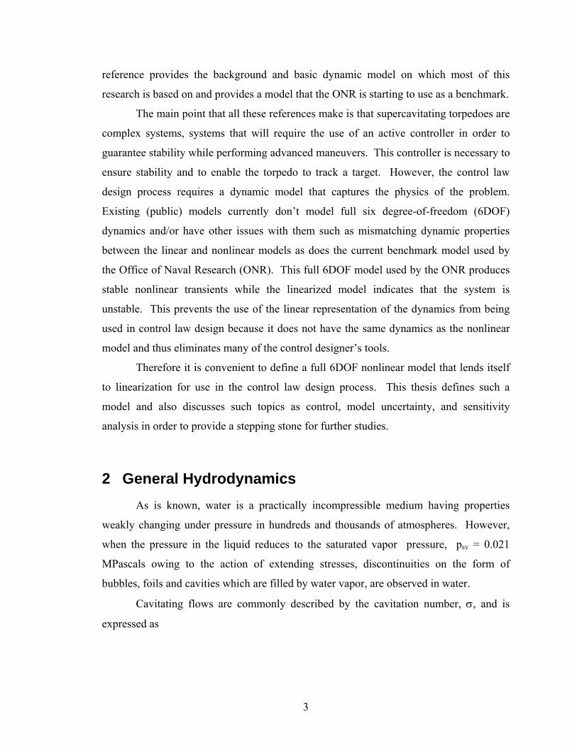
Cavitating flows are commonly described by the cavitation number, σ, and is

expressed as

3

2

c

21 V

pp

ρσ −= ∞ Equation 1

where ρ is the fluid density, V is the free-stream velocity, and and are the ambient

and cavity pressures, respectively. According to the degree, or size of σ, three cavitation

stages are defined:

∞p cp

1. Initial cavitation is the bubble stage and it is accompanied by the strong

characteristic noise of collapsing bubbles and is capable of destroying solid

material; for example, blades of screws, pumps, turbines.

2. Partial cavitation is the stage when arising cavities cover a cavitating body part.

The cavity pulses and is unstable.

3. Fully developed cavitation – supercavitation is the stage when the cavity

dimensions considerably exceed the body dimensions.

These stages are better illustrated in Figure 1. This figure shows a fictional cavitation

experiment that holds the velocity constant and allows varying amounts of ambient

pressure; various amounts of cavitation can be observed.

Figure 1: Schematic of Cavitation Flow Regimes [6]

4

Here, σi can be thought of as a type of performance boundary where iσσ > results in no

cavitation. For this study, the cavitation number is assumed constant, σ = 0.029, which is

low enough for natural supercavitation to occur.

Noncavitating flows occur at sufficiently high pressures. Supercavitation occurs

at very low pressures where a very long vapor cavity exists and in many cases the cavity

wall appears glassy and stable except near the end of the cavity. Limited cavitation is

seen between these two flow regimes.

Other parameters used to describe the supercavitating flows are the Froude (Fr)

number and the ventilation coefficient (CQ) and are shown below (respectively).

cavgD

V=Fr Equation 2

2cavVD

QCQ = Equation 3

Here g is the gravitational acceleration, the cavitator diameter is Dcav, V is the magnitude

of the vehicle’s velocity vector, and Q is the volumetric rate at which ventilation gas is

supplied to the cavity. The Froude number characterizes the importance of gravity to the

flow, and therefore governs distortions to the nominally axis-symmetric cavity centerline

shape. The ventilation coefficient governs the time-dependent behavior of the cavity as

ventilation gas is entrained by the flow. For the trajectories considered in this thesis, the

Froude number is typically on the order of 90 to 110. [1]

A supercavity can be maintained in one of two ways: (1) achieving such a high

speed that the water vaporizes near the nose of the body; or, (2) supplying gas to the

cavity at nearly ambient pressure. The first technique is known as vaporous or natural

cavitation. The second is termed ventilation, or artificial, cavitation. Note that each

concept involves some sort of cavitator with a clean edge to provide the sharp drop in

pressure required to form a clean cavity near the nose of the body. For simplicity, only

natural cavitation is considered in this thesis and thus the ventilation coefficient is zero.

It is, however, conceivable to think of controlling the ventilation, and thus the cavitation

number to affect the dynamics of the system. The effects of varying cavitation numbers

will be described in Section 8.1.1.

5

3 Vehicle Dynamics As was mentioned in the introduction, the bulk of this dynamic model is based on,

and expanded from, the work done by Ivan Kirschner et. al. at Anteon Corp under

direction of the ONR. For completeness, all the dynamics will be described in detail

here.

3.1 Coordinate System, States, and Control Variables

The model developed by Anteon uses the cavitator pivot point as the torpedo's

origin. However, for simplicity and for reasons of common convention, this thesis

computes the dynamics with the torpedo’s center of gravity as the origin.

The coordinate system was chosen to be the same as is defined by Kirschner et.

al. That is, ξ is positive forward of the center of mass, η is positive to the starboard

portion of the torpedo, and h is positive, as is defined by the right-hand rule, down. This

coordinate system will make up the body coordinate system. The symbols used

throughout the text correspond generally to current usage and are used in a consistent

manner.

The states of the system are the body component states, one set of the two widely

used. The two different choices can be seen in Table 1.

6

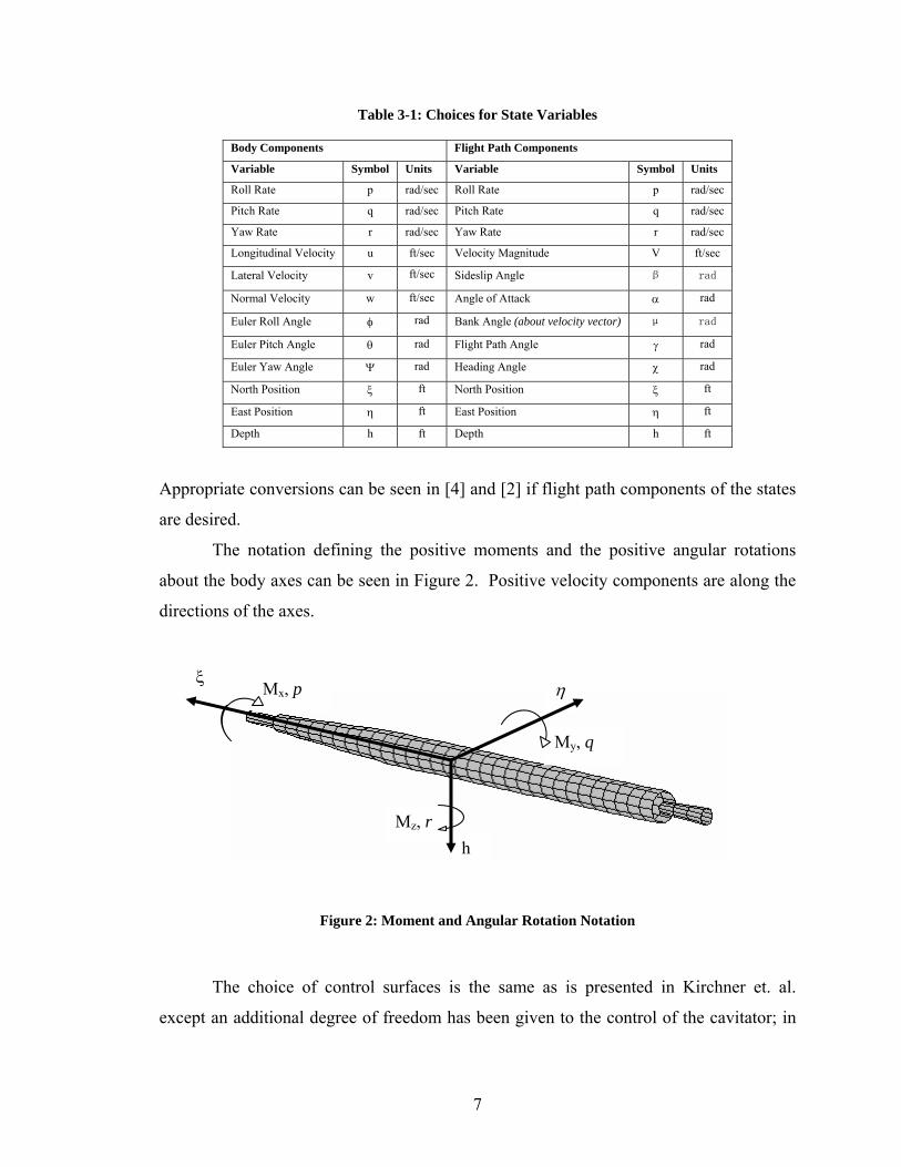
Table 3-1: Choices for State Variables

Body Components Flight Path Components

Variable Symbol Units Variable Symbol Units

Roll Rate p rad/sec Roll Rate p rad/sec

Pitch Rate q rad/sec Pitch Rate q rad/sec

Yaw Rate r rad/sec Yaw Rate r rad/sec

Longitudinal Velocity u ft/sec Velocity Magnitude V ft/sec

Lateral Velocity v ft/sec Sideslip Angle β rad

Normal Velocity w ft/sec Angle of Attack α rad

Euler Roll Angle φ rad Bank Angle (about velocity vector) μ rad

Euler Pitch Angle θ rad Flight Path Angle γ rad

Euler Yaw Angle Ψ rad Heading Angle χ rad

North Position ξ ft North Position ξ ft

East Position η ft East Position η ft

Depth h ft Depth h ft

Appropriate conversions can be seen in [4] and [2] if flight path components of the states

are desired.

The notation defining the positive moments and the positive angular rotations

about the body axes can be seen in Figure 2. Positive velocity components are along the

directions of the axes.

Mz, r

My, q

Mx, p

h

η ξ

Figure 2: Moment and Angular Rotation Notation

The choice of control surfaces is the same as is presented in Kirchner et. al.

except an additional degree of freedom has been given to the control of the cavitator; in

7

addition of pivoting in the pitch axis, rotation in the yaw axis has also been considered in

the equations of motion.

Therefore, our states and controls are:

[ ]Trqpwvuhx ψθφηξ=

[ ]yawpitch cavcavffff δδδδδδ

4321=Δ

However, since the water density variation with depth is not modeled in this

investigation, all the position states, North, East, and depth position states, are just

kinematics and play no role in the dynamics modeled below. The state vector then

becomes

[ ]Trqpwvux ψθφ=

3.1.1 Flow Angles

It is useful to define the orientation of the torpedo about the velocity vector as

these values are often used to compute the forces and moments acting on the body. The

inclination of the body to the velocity vector is defined by the angle of attack and the

sideslip angle such that

uw1tan −=α Equation 4

222

1sinwvu

v

++= −β Equation 5

3.1.2 Torpedo Dimensions

Simulation was conducted on a vehicle with the following characteristics: 4.0 m

in length, 0.2 m in diameter, and with a cavitator diameter of 0.07 m. The fins were

located 3.5 m aft of the cavitator, and were swept back at 45º. Although the mass

8

properties of the vehicle will change as the rocket and ventilation fuels are consumed,

they are assumed constant for purposes of the current analysis. This model is an Applied

Research Lab (ARL) defined model.

3.2 Cavity Dynamics

The behavior of the cavity is central to the dynamics of a supercavitating vehicle.

It is the cavity that makes this dynamical system not only highly nonlinear, but dependent

on the history of the vehicle’s motion. The nominally steady cavity behavior forms the

basis of the quasi-time dependent model implemented for the current investigation. The

cavity model not only affects the forces acting at the nose of the vehicle, but also has a

strong influence on the fin forces and moments via the amount the fins are immersed in

the free-stream flow and the planing forces, both of which will be discussed in more

detail later in the thesis.

During supercavitation, the cavity stays attached to the body and the cavity

closure is far downstream. The length of the cavity does not vary significantly even

though considerable oscillations can occur at its closure. However, the cavity acts as if it

were an extension of the body. In this case, the same flow field would exist around a

solid body having a shape comprising of the wetted nose plus the free-cavity profile as

might be see in Figure 3.

Figure 3: Artists Conception of a Supercavitating Torpedo

9

3.2.1 Maximum Cavity Dimensions

The cavity itself is slender, and its maximum diameter is at least 5 times greater

than the cavitator diameter. For axis-symmetric flows, the maximum cavity diameter

(made dimensionless with the cavitator diameter) is a strong function of the cavitator

drag coefficient and the cavitation number, and is otherwise nearly independent of the

cavitator shape (Reichardt, 1946). In fact, both the cavity diameter and the cavity length

increase with cavitator drag and decrease with cavitation number.

Various analytical, numerical, and semi- and fully-empirical models have been

developed that provide estimates of the maximum cavity radius, Rc, and cavity length, Lc.

The analytical formulae of Reichardt (1946) provide useful and reasonably accurate1

approximations for investigation of cavity dynamics. These relations can be seen in

Equations 6-7.

( )2028.01*0

σσ ++= DD CC Equation 6

93.035.1 −= σDcavc CRR Equation 7

( 6.024.1 123.1 −= −σDcavc CDL )

Equation 8

where , R.8050.00

constCD == cav is the cavitator radius, and Dcav is the cavitator

diameter.

It is important to note that since the cavitation number σ is assumed constant for

this investigation, the drag coefficient is considered constant. This means that the

maximum cavity length and radius is assumed constant and will also affect the way that

the cavitator forces are computed. This is a very large assumption since physics dictate

that the cavitation number is going to change as the velocity and cavity change.

3.2.2 Cavity Centerline

There are essentially three methods (which are practical for time-based

simulations) to compute the cavity centerline: (1) Analytical formula developed by

Münzer and Reichardt (1950) which are described in the paper by Kirschner [1], (2)

1 The approximations are accurate for completely horizontal flows only.

10

“Classic” displacement equations based on acceleration, and (3) Use of past (delayed)

position states2 which are “coincident with the cavity centerline.” Let us first consider

the first two methods which are a function of the instantaneous states.

If the analytical formulas of Münzer and Reichardt as presented by Kirschner [1]

are used, the local cavity radius, η-, and h-offsets for a given distance behind the

cavitator are given in Equations 9-11, respectively.

4.21

2

cavc

cavccav

2/2//

1⎥⎥⎦

⎤

⎢⎢⎣

⎡⎟⎟⎠

⎞⎜⎜⎝

⎛ −−=

DLDLDx

Rr cc Equation 9

2

cav

turn2c Fr

1)( ⎟⎟⎠

⎞⎜⎜⎝

⎛=

Dx

ga

xη Equation 10

2

cav

g2c Fr

1)( ⎟⎟⎠

⎞⎜⎜⎝

⎛−=

Dx

ga

xh Equation 11

where Fr is the Froude number, g is gravity, aturn is the apparent turn acceleration and ag

is the apparent tail-up acceleration of the cavity (which are both functions of the states).

ag is also a function of buoyancy, 8.29 m/s2. Although distortions to the cavity shape due

to turning and gravity have been considered, distortions associated with cavitator lift have

been ignored. For more information on how pitching the cavitator can affect cavity

dimensions see reference [9].

If the classic physics equations are used, η- and h-offsets are calculated by

Equations 12-13.

( )2

21 ⎟

⎠⎞

⎜⎝⎛=Vxax turncη Equation 12

( )2

21 ⎟

⎠⎞

⎜⎝⎛−=Vxaxh gc Equation 13

Figure 4 shows the drastic difference between the analytical set of equations (Eq.’s 10 &

11) derived by Munzer and Reichardt and the classic displacement equations (Eq’s 12 &

2 Position states (ξ, η, and h) were the option chosen by the researchers at Anteon, though they are not the only option. Delayed Euler angles would be another suitable option.

11

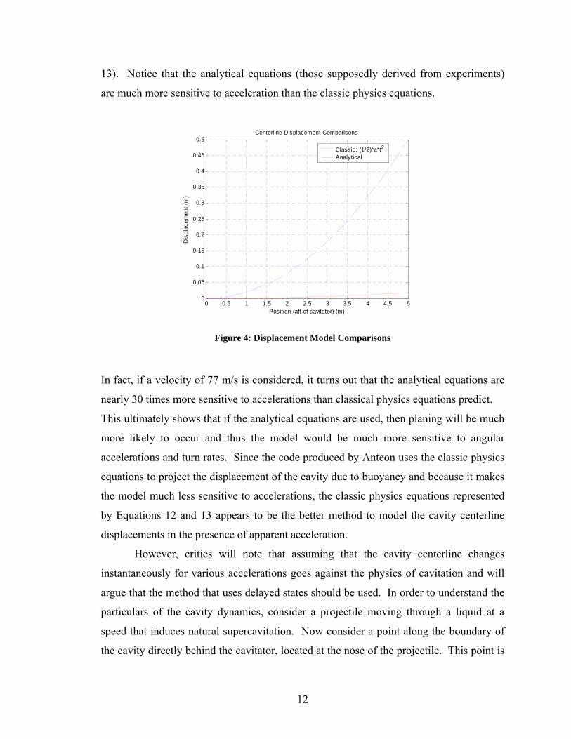
13). Notice that the analytical equations (those supposedly derived from experiments)

are much more sensitive to acceleration than the classic physics equations.

0 0.5 1 1.5 2 2.5 3 3.5 4 4.5 50

0.05

0.1

0.15

0.2

0.25

0.3

0.35

0.4

0.45

0.5Centerline Displacement Comparisons

Position (aft of cavitator) (m)

Dis

plac

emen

t (m

)

Classic: (1/2)*a*t2

Analytical

Figure 4: Displacement Model Comparisons

In fact, if a velocity of 77 m/s is considered, it turns out that the analytical equations are

nearly 30 times more sensitive to accelerations than classical physics equations predict.

This ultimately shows that if the analytical equations are used, then planing will be much

more likely to occur and thus the model would be much more sensitive to angular

accelerations and turn rates. Since the code produced by Anteon uses the classic physics

equations to project the displacement of the cavity due to buoyancy and because it makes

the model much less sensitive to accelerations, the classic physics equations represented

by Equations 12 and 13 appears to be the better method to model the cavity centerline

displacements in the presence of apparent acceleration.

However, critics will note that assuming that the cavity centerline changes

instantaneously for various accelerations goes against the physics of cavitation and will

argue that the method that uses delayed states should be used. In order to understand the

particulars of the cavity dynamics, consider a projectile moving through a liquid at a

speed that induces natural supercavitation. Now consider a point along the boundary of

the cavity directly behind the cavitator, located at the nose of the projectile. This point is

12

stationary in the ξ-axis. In other words, the projectile moves, not the boundary. Now this

point is a function of the current states of the projectile. By the time the projectile has

moved and its states have changed, the point along the boundary still is associated with

the original states and is now relatively further behind the cavitator. This delay in states

has an overall effect on the dynamics, but the question is how much?

To answer this, a Dutch-Roll3 model with the slide-slip angle and yaw rate used

as the representative states of the torpedo is considered. After the torpedo dynamics are

identified, two methods are created to compute the cavity centerline; the “simple” model

uses the classic displacement equations mentioned above, and the second, more complex

model, uses a set of delayed states. The number of delays needed for each state is

dependent upon the number of sections the model designer wants to divide the cavity

profile into; in this case ten sections were chosen and the delays are then assumed to be

variable time delays that are dependent upon the velocity of the torpedo. Interpolation

techniques can then be used to find data between the specified sections. Note that the

more sections that the cavity is divided into, the more accurate the cavity dimensions can

be calculated at any given point behind the cavitator.

In order to take the delays of the more complex system into consideration, it is

common practice to use a nonlinear 2nd order Padé approximation4 to model this delay.

This not only ensures that the delays are represented in the model, but also guarantees

that the delays are differentiable. A 2nd order approximation is given by the transfer

function written in Equation 14.

( )( ) 1221

12212

2

sssse s

τττττ

+++−

≅− Equation 14

where τ is the time delay given in seconds.

The consequence of using these approximations is that it adds two poles and

zeros5 to the linear model for every Padé approximation used. This ultimately affects the

3 There are many sources out there that describe how to model the Dutch-Roll dynamics. One of these is by Etkin [2]. 4 Other models have tried to model these delays through use of a “state buffer” in which the states are stored in an array and then accessed in the functions. This is potentially dangerous as it can result in misrepresentation of the nonlinear dynamics during linearization. 5 Poles, zeros, and other linearization information are described in more depth later in the thesis.

13

stability and controllability of the linear state-space representation of the nonlinear

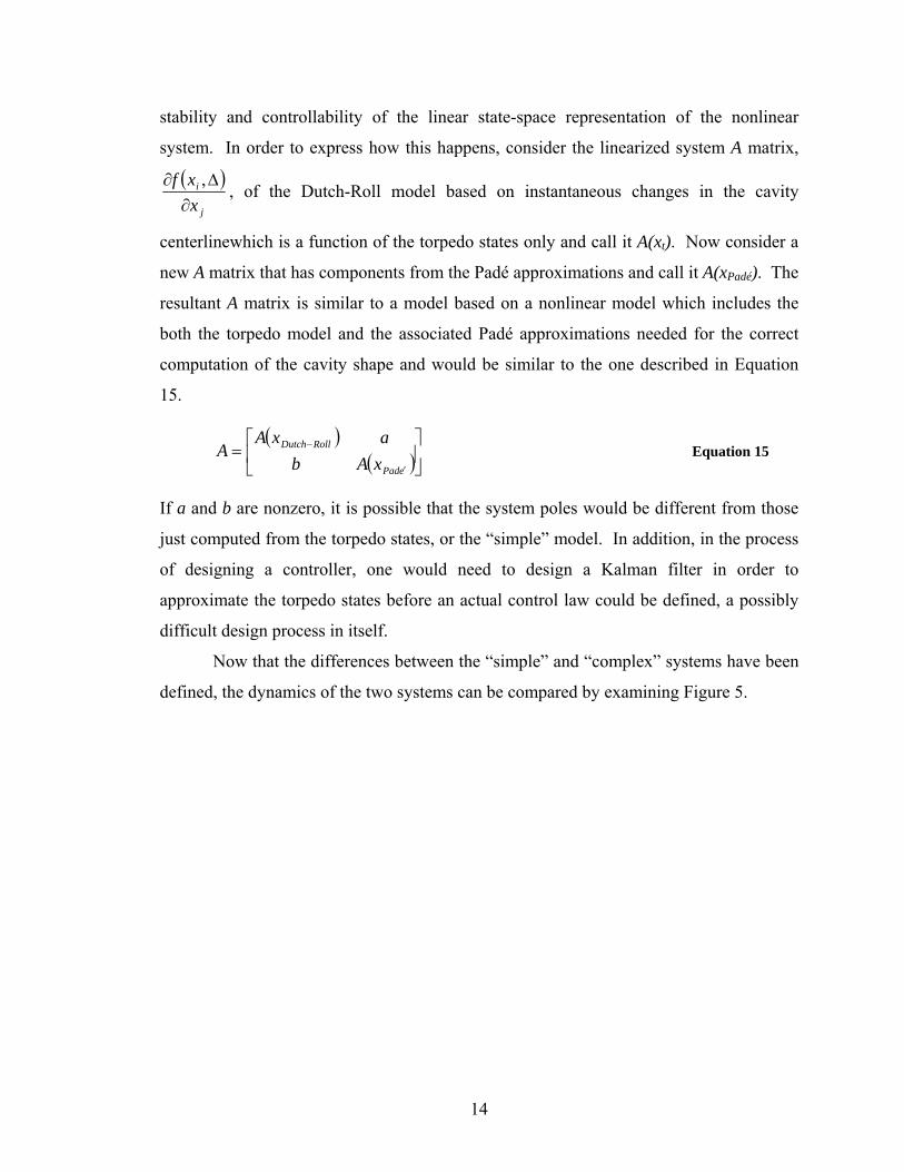
system. In order to express how this happens, consider the linearized system A matrix,

( )j

i

xxf∂

Δ∂ ,, of the Dutch-Roll model based on instantaneous changes in the cavity

centerlinewhich is a function of the torpedo states only and call it A(xt). Now consider a

new A matrix that has components from the Padé approximations and call it A(xPadé). The

resultant A matrix is similar to a model based on a nonlinear model which includes the

both the torpedo model and the associated Padé approximations needed for the correct

computation of the cavity shape and would be similar to the one described in Equation

15.

Equation 15 ( )

( ⎥⎦

⎤⎢⎣

⎡=

′

−

ePad

RollDutch

xAbaxA

A )

If a and b are nonzero, it is possible that the system poles would be different from those

just computed from the torpedo states, or the “simple” model. In addition, in the process

of designing a controller, one would need to design a Kalman filter in order to

approximate the torpedo states before an actual control law could be defined, a possibly

difficult design process in itself.

Now that the differences between the “simple” and “complex” systems have been

defined, the dynamics of the two systems can be compared by examining Figure 5.

14

-100 -90 -80 -70 -60 -50 -40 -30 -20 -10 0-60

-40

-20

0

20

40

600.84 0.72 0.58 0.44 0.140.3

0.44 0.3 0.14

0.92

0.98

0.92

0.72 0.580.84

80

0.98

204060

Delayed States Method PolesDelayed States Method Zeros"Classic" Method Poles

Pole-Zero Map: Centerline Method Comparison

Real Axis

Imag

inar

y Ax

is

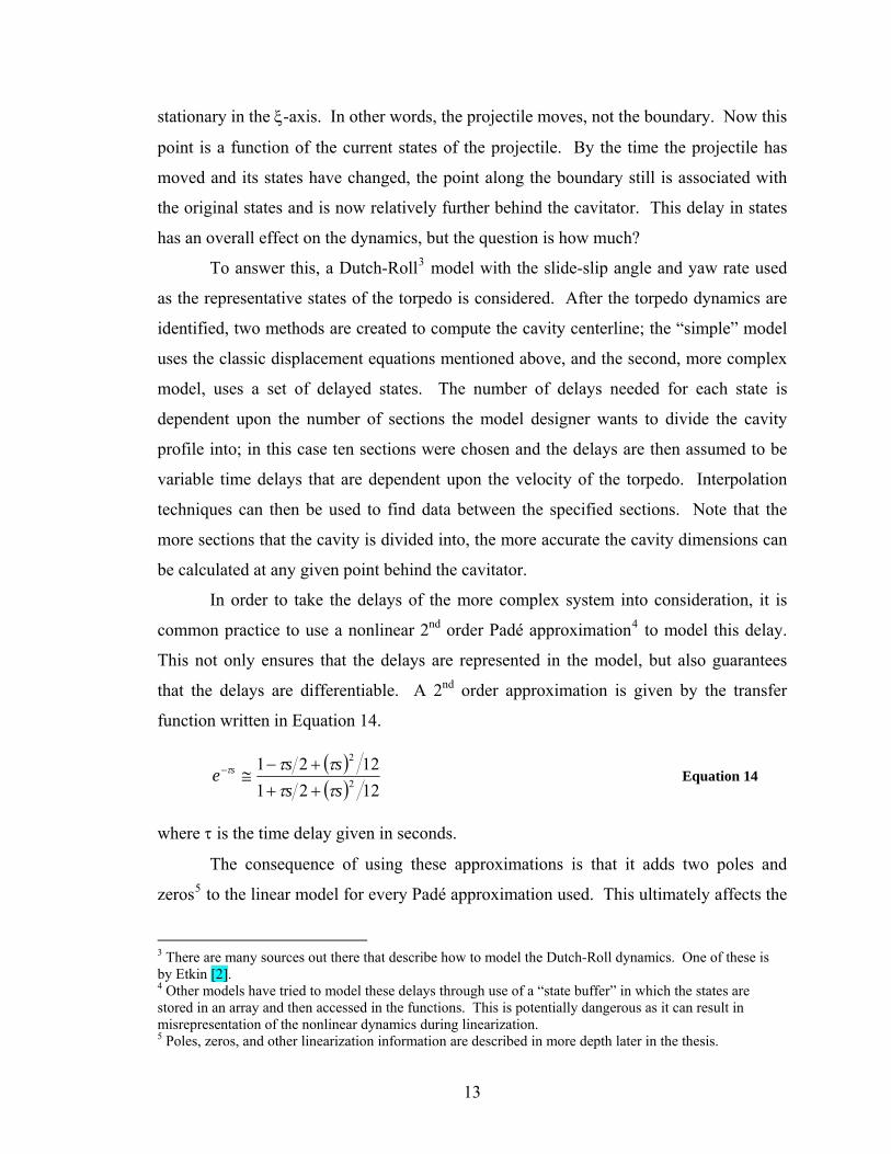
Figure 5: Pole Comparison of Systems with Delays vs. "Classic" Centerline Displacement

The dynamics of interest in this graph are shown in the RHP. These poles represent the

dominating dynamics of the two systems. Note that the two poles lie in nearly the same

location. This means that the extra states associated with the 20 delays (ten for each

state, some not shown in the above graph) have little influence on the torpedo’s motion

(assuming that the steady-state gains are equal). What it also means is that it is

reasonable6 to use the “classic” displacement equations which are dependent upon the

instantaneous states to compute the distortion of the cavity centerline.

3.2.3 Cavity Closure

A description of the cavity closure zone is the most difficult issue when

describing cavity shape and how it affects the overall cavity dynamics. According to the

6 There is some concern that it will not match in the pitch axis because of the buoyancy forces acting on the cavity, but the same type of pole matching seen in Figure 5 occurs with a 1-g turn trim condition, a condition similar to straight-and-level flight with buoyancy affecting the cavity shape in the vertical direction. This leads us to the assumption that the delays will have a similar effect on a full 6DOF.

15

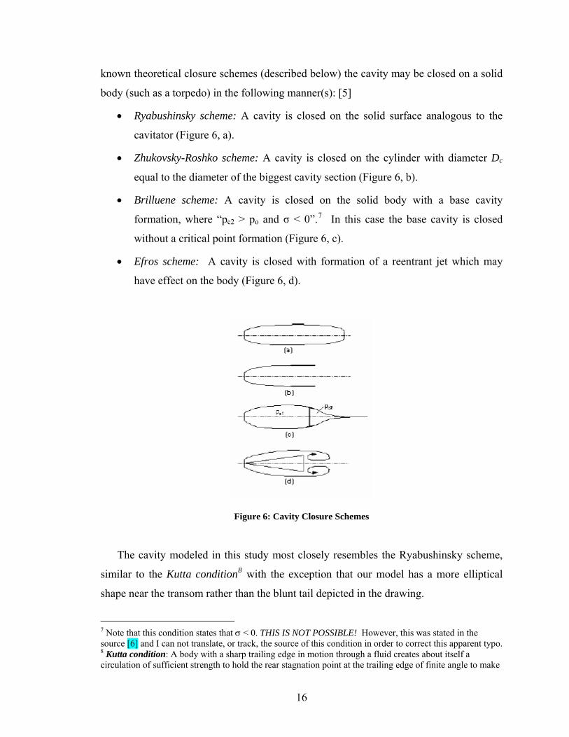
known theoretical closure schemes (described below) the cavity may be closed on a solid

body (such as a torpedo) in the following manner(s): [5]

• Ryabushinsky scheme: A cavity is closed on the solid surface analogous to the

cavitator (Figure 6, a).

• Zhukovsky-Roshko scheme: A cavity is closed on the cylinder with diameter Dc

equal to the diameter of the biggest cavity section (Figure 6, b).

• Brilluene scheme: A cavity is closed on the solid body with a base cavity

formation, where “pc2 > po and σ < 0”.7 In this case the base cavity is closed

without a critical point formation (Figure 6, c).

• Efros scheme: A cavity is closed with formation of a reentrant jet which may

have effect on the body (Figure 6, d).

Figure 6: Cavity Closure Schemes

The cavity modeled in this study most closely resembles the Ryabushinsky scheme,

similar to the Kutta condition8 with the exception that our model has a more elliptical

shape near the transom rather than the blunt tail depicted in the drawing.

7 Note that this condition states that σ < 0. THIS IS NOT POSSIBLE! However, this was stated in the source [6] and I can not translate, or track, the source of this condition in order to correct this apparent typo. 8 Kutta condition: A body with a sharp trailing edge in motion through a fluid creates about itself a circulation of sufficient strength to hold the rear stagnation point at the trailing edge of finite angle to make

16

3.2.4 Final Cavity Shape

When all is said and done, the following ellipsoid represents the cavity shape

(with no other accelerations except buoyancy):

0 0.5 1 1.5 2 2.5 3 3.5 4 4.5-1

0

1Cavity Shape

y c

0 0.5 1 1.5 2 2.5 3 3.5 4 4.5-0.015

-0.01

-0.005

0

z c

0 0.5 1 1.5 2 2.5 3 3.5 4 4.50

0.1

0.2

r c

x

Figure 7 : Cavity Shape Components

Figure 8: Overall Cavity Shape

the flow along the trailing edge bisector angle smooth. For a body with a cusped trailing edge where the upper and lower surfaces meet tangentially, a smooth flow at the trailing edge requires equal velocities on both sides of the edge in the tangential direction. Essentially it means that there can be no velocity discontinuities at the trailing edge, or in this case, the transom (rear) of the cavity.

17

Remember that a negative h-value means “up.” If the torpedo were making a starboard

turn, the η-component of the cavity centerline would be nonzero and positive and similar

in shape to the h-component.

3.3 Cavitator Forces

Throughout this study of the supercavitating torpedo dynamics, several attempts

were made to describe the disk-cavitator forces. The first attempt didn’t proportionally

take into consideration the cavitator’s relative angle of attack or bank angle and the

second failed to model the lift and side forces correctly. However, by taking the apparent

flow angles into account (as shown in Figure 9), the cavitator forces can be computed as

a function of the disk’s “perpendicular” force, apparent angle of attack and apparent

sideslip angle.

βcav Fp

αcav

zcav

ycav

xbody

xcavybody

zbody

Figure 9: Cavitator Free-Body Diagram

where

( ) Dcavp CRVF 2221 πρ= Equation 16

pitchcavcav

cavwvu

qlδαα −

++−=

222 Equation 17

yawcavcav

cavwvu

rlδββ −

++−=

222 Equation 18

18

Fp is the “perpendicular” force acting on the cavitator, and lcav is the distance from the

cavitator to the origin of the system (in this case, the distance to the center of gravity). Fp

is considered perpendicular because the equation used to compute the force is based on

flows that are perpendicular to the cavitator disc.

The body components of the cavitator forces then become:

⎥⎥⎥

⎦

⎤

⎢⎢⎢

⎣

⎡−=

⎥⎥⎥

⎦

⎤

⎢⎢⎢

⎣

⎡

=

cavcavp

cavp

cavcavp

cav

cav

cav

cav

FF

F

FFF

F

z

y

x

βαβ

βα

cossinsin

coscos Equation 19

The moments acting about the cavitator’s center of effect are assumed to be

negligible, but the moment about the center of gravity due to the forces is not. Since the

origin of the system is the center of gravity and the center of gravity is assumed to lie on

the ξ-axis, the moment arm, lcav, is equal to the location of the center of mass (xcg) and is

measured as the distance aft of the nose of the torpedo. Therefore, the moments

produced by the cavitator forces are:

[ ] cavT

cgcav FxM ×= 00 Equation 20

Remember that the assumption was made that the drag coefficient remains

constant and so Fp is always constant if the velocity is held constant. This means that the

cavitator forces and moments are only going to be a function of the apparent flow angles

cavα and cavβ .

In order to get a better idea of both the sign convention and sensitivity of the

cavitator forces to the apparent flow angles, a straight-and-level flight condition with a

velocity of 77 m/s is considered and cavα and cavβ are allowed to vary.

19

-20 -15 -10 -5 0 5 10 15 20-15000

-10000

-5000

0

5000

F cav

Cavitator Forces - α Test

-20 -15 -10 -5 0 5 10 15 20-1

-0.5

0

0.5

1x 10

4

α (deg)

Mca

v

Cavitator Moments - α Test

FxFyFz

MxMyMz

Figure 10: Cavitator Forces and Moments - α Test

Notice from Figure 10 that the forces and moments are “centered” about a negative cavα

value. This means that the cavitator has to be pitched down or the angle of attack as to be

negative in order to provide the lift force needed to help support the weight of the torpedo

since fin or planing forces would be insufficient to support the weight alone and since a

controllable forward force is necessary for active control.

Figure 11 shows the effects of varying cavβ values.

20

-20 -15 -10 -5 0 5 10 15 20-15000

-10000

-5000

0

5000

F cav

Cavitator Forces - β Test

-20 -15 -10 -5 0 5 10 15 20-1

-0.5

0

0.5

1x 10

4

β (deg)

Mca

v

Cavitator Moments - β Test

FxFyFz

MxMyMz

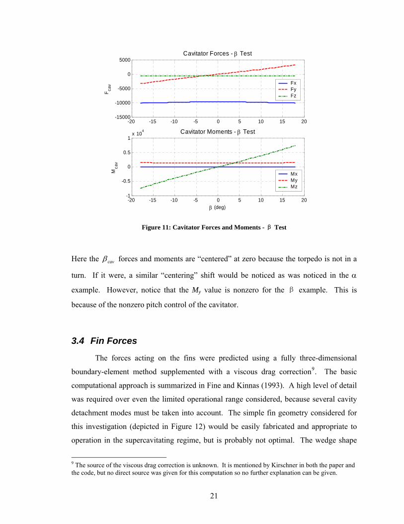
Figure 11: Cavitator Forces and Moments - β Test

Here the cavβ forces and moments are “centered” at zero because the torpedo is not in a

turn. If it were, a similar “centering” shift would be noticed as was noticed in the α

example. However, notice that the My value is nonzero for the β example. This is

because of the nonzero pitch control of the cavitator.

3.4 Fin Forces

The forces acting on the fins were predicted using a fully three-dimensional

boundary-element method supplemented with a viscous drag correction9. The basic

computational approach is summarized in Fine and Kinnas (1993). A high level of detail

was required over even the limited operational range considered, because several cavity

detachment modes must be taken into account. The simple fin geometry considered for

this investigation (depicted in Figure 12) would be easily fabricated and appropriate to

operation in the supercavitating regime, but is probably not optimal. The wedge shape

9 The source of the viscous drag correction is unknown. It is mentioned by Kirschner in both the paper and the code, but no direct source was given for this computation so no further explanation can be given.

21

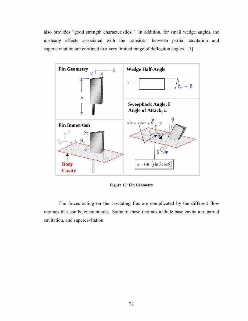
also provides “good strength characteristics.” In addition, for small wedge angles, the

unsteady effects associated with the transition between partial cavitation and

supercavitation are confined to a very limited range of deflection angles. [1]

L

S

Wedge Half-AngleFin Geometry

Fin Immersion

Sweepback Angle, θ Angle of Attack, α

[ ]θδα cossinsin 1−=

δ

So

Figure 12: Fin Geometry

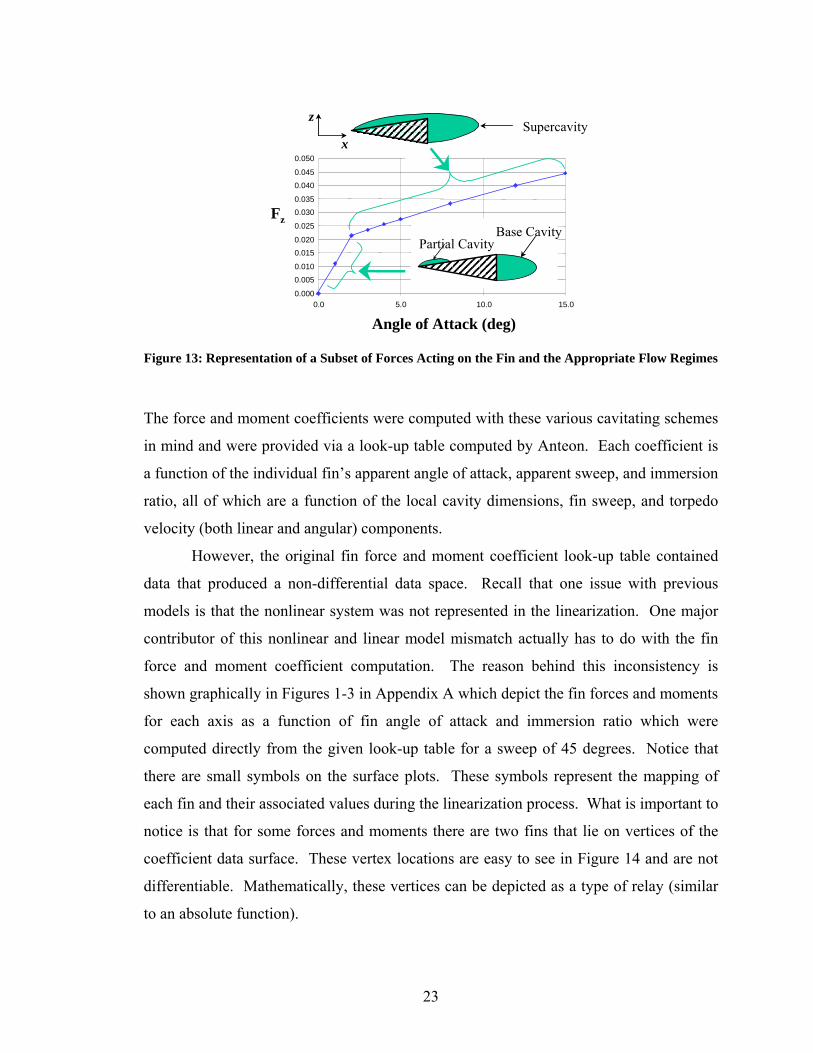
The forces acting on the cavitating fins are complicated by the different flow

regimes that can be encountered. Some of these regimes include base cavitation, partial

cavitation, and supercavitation.

BodyCavity

x

y

zx

y

z

θ

β

Inflow velocity, Vρ

22

0.000

0.005

0.010

0.0150.020

0.025

0.0300.035

0.040

0.045

0.050

0.0 5.0 10.0 15.0

Fz

Angle of Attack (deg)

Partial CavityBase Cavity

Supercavityx

z

Figure 13: Representation of a Subset of Forces Acting on the Fin and the Appropriate Flow Regimes

The force and moment coefficients were computed with these various cavitating schemes

in mind and were provided via a look-up table computed by Anteon. Each coefficient is

a function of the individual fin’s apparent angle of attack, apparent sweep, and immersion

ratio, all of which are a function of the local cavity dimensions, fin sweep, and torpedo

velocity (both linear and angular) components.

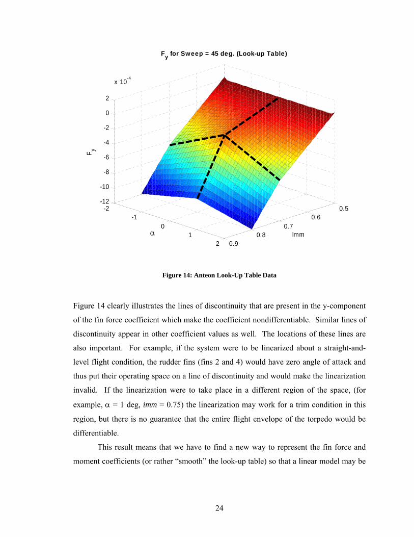
However, the original fin force and moment coefficient look-up table contained

data that produced a non-differential data space. Recall that one issue with previous

models is that the nonlinear system was not represented in the linearization. One major

contributor of this nonlinear and linear model mismatch actually has to do with the fin

force and moment coefficient computation. The reason behind this inconsistency is

shown graphically in Figures 1-3 in Appendix A which depict the fin forces and moments

for each axis as a function of fin angle of attack and immersion ratio which were

computed directly from the given look-up table for a sweep of 45 degrees. Notice that

there are small symbols on the surface plots. These symbols represent the mapping of

each fin and their associated values during the linearization process. What is important to

notice is that for some forces and moments there are two fins that lie on vertices of the

coefficient data surface. These vertex locations are easy to see in Figure 14 and are not

differentiable. Mathematically, these vertices can be depicted as a type of relay (similar

to an absolute function).

23

0.50.6

0.70.8

0.9

-2-1

01

2

-12

-10

-8

-6

-4

-2

0

2

x 10-4

Imm

Fy for Sweep = 45 deg. (Look-up Table)

α

F y

Figure 14: Anteon Look-Up Table Data

Figure 14 clearly illustrates the lines of discontinuity that are present in the y-component

of the fin force coefficient which make the coefficient nondifferentiable. Similar lines of

discontinuity appear in other coefficient values as well. The locations of these lines are

also important. For example, if the system were to be linearized about a straight-and-

level flight condition, the rudder fins (fins 2 and 4) would have zero angle of attack and

thus put their operating space on a line of discontinuity and would make the linearization

invalid. If the linearization were to take place in a different region of the space, (for

example, α = 1 deg, imm = 0.75) the linearization may work for a trim condition in this

region, but there is no guarantee that the entire flight envelope of the torpedo would be

differentiable.

This result means that we have to find a new way to represent the fin force and

moment coefficients (or rather “smooth” the look-up table) so that a linear model may be

24

computed in order to understand the system properties and to facilitate a (linear) control

law design.

In order to make the fin operating space completely differentiable for all flow

conditions, a parabolic least squares function was fitted to each of the fin force and

moment coefficients. This involves a least-squares type approximation to the fin force

and moment data provided by Anteon such that ( )fMF swpimmfCC ,,, α= . Since the

data is not completely linear, it makes sense to fit a higher order equation to the data. In

indicial notation:

+⋅⋅+⋅⋅+⋅+⋅= 24

23

32

31, jijijiji immpimmpimmppC ααα

8765 pimmppimmp jiji +⋅+⋅+⋅⋅ αα

Equation 21

Note that the higher the order of the approximation, the more accurate the approximation

will be.

In order to solve for the coefficients pi the system can be solved as follows:

First define the vectors as follows

⎥⎥⎥⎥

⎦

⎤

⎢⎢⎢⎢

⎣

⎡

=

8

8

1

p

pp

PΜ

⎥⎥⎥⎥⎥⎥⎥⎥⎥⎥⎥

⎦

⎤

⎢⎢⎢⎢⎢⎢⎢⎢⎢⎢⎢

⎣

⎡

⋅⋅⋅

=

1

2

2

3

3

j

i

ji

ji

ji

j

i

imm

immimmimm

imm

A

αααα

α

jiCB ,=

Now the coefficients pi can be solved…

[ ][ ] BAAAP

BAPAABPA

TT

TT

1−===⋅

Equation 22

25

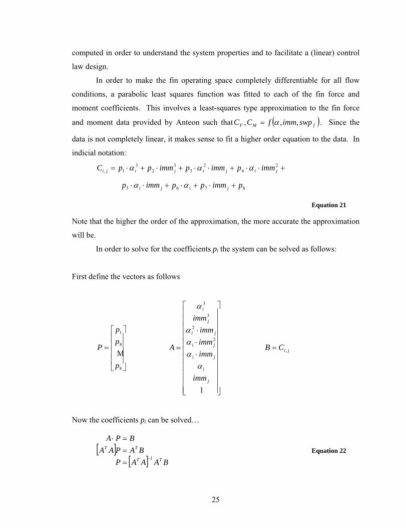
To get a measure of how good the approximation is to the original data, an averaged

value representing the %-error can be computed using Equation 23.

B

BPAE

−⋅= Equation 23

Note that these approximations must be done for each coefficient.

Using this method, the coefficients pi and their representative %-errors can be

seen in Tables 2 & 3.

Coefficient p1 p2 p3 p4

Fx 0.0000E+00 5.0856E-03 4.6230E-05 0.0000E+00Fy 0.0000E+00 -4.8993E-03 -4.4502E-05 0.0000E+00Fz -6.5104E-06 0.0000E+00 0.0000E+00 1.0074E-02Mx -2.6977E-06 0.0000E+00 0.0000E+00 1.3920E-03My 2.1674E-06 0.0000E+00 0.0000E+00 -1.6503E-03Mz 0.0000E+00 -1.1683E-03 -4.0303E-05 0.0000E+00

Coefficient p5 p6 p7 p8Fx 0.0000E+00 0.0000E+00 5.6605E-04 -4.7508E-04Fy 0.0000E+00 0.0000E+00 1.0178E-03 1.7334E-04Fz -1.3193E-03 2.6340E-04 0.0000E+00 0.0000E+00Mx 2.1428E-03 -2.8316E-04 0.0000E+00 0.0000E+00My -1.8498E-03 2.7272E-04 0.0000E+00 0.0000E+00Mz 0.0000E+00 0.0000E+00 -1.4744E-03 5.8590E-04

Table 3-2: Equation Coefficient Values

Coefficient % Error

Fx 12.99%Fy 16.71%Fz 11.06%Mx 14.53%My 13.90%Mz 17.92%

Table 3-3: Coefficient %-Errors

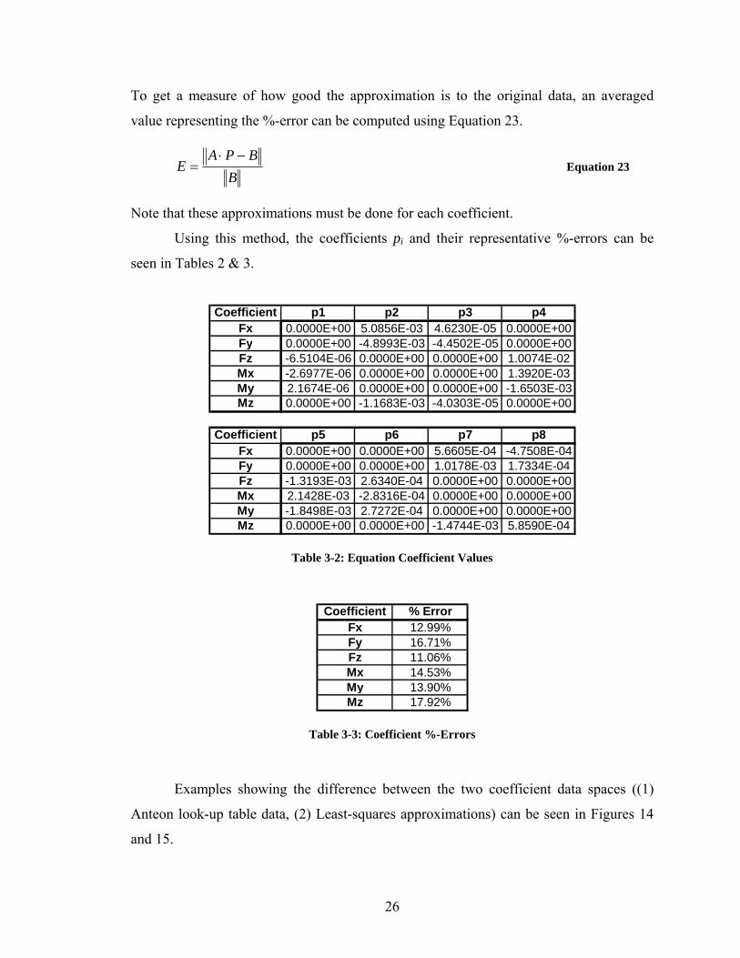
Examples showing the difference between the two coefficient data spaces ((1)

Anteon look-up table data, (2) Least-squares approximations) can be seen in Figures 14

and 15.

26

0.50.6

0.70.8

0.9

-2-1

01

2

-15

-10

-5

0

5

x 10-4

Imm

Fy for Sweep = 45 deg. (Least Squares Fit)

α

F y

Figure 15: Coefficient Data Using Least Squares Approximations

Figure 15 shows that by taking a least squares approximate fit to the data, the lines of

discontinuities are removed and the entire operating space of the fins would be

differentiable.

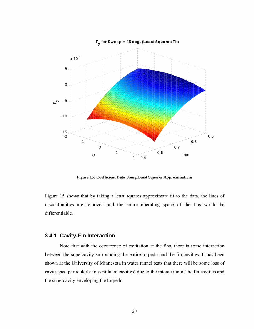
3.4.1 Cavity-Fin Interaction

Note that with the occurrence of cavitation at the fins, there is some interaction

between the supercavity surrounding the entire torpedo and the fin cavities. It has been

shown at the University of Minnesota in water tunnel tests that there will be some loss of

cavity gas (particularly in ventilated cavities) due to the interaction of the fin cavities and

the supercavity enveloping the torpedo.

27

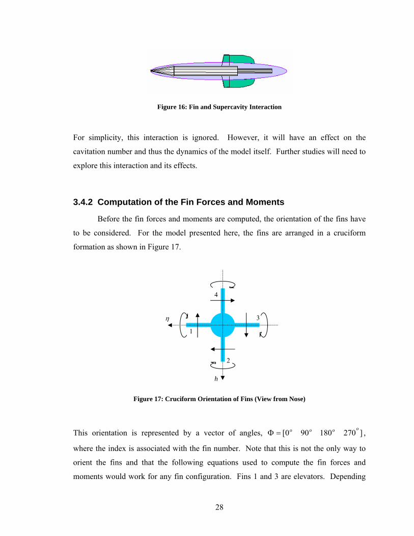
Figure 16: Fin and Supercavity Interaction

For simplicity, this interaction is ignored. However, it will have an effect on the

cavitation number and thus the dynamics of the model itself. Further studies will need to

explore this interaction and its effects.

3.4.2 Computation of the Fin Forces and Moments

Before the fin forces and moments are computed, the orientation of the fins have

to be considered. For the model presented here, the fins are arranged in a cruciform

formation as shown in Figure 17.

4

3 η

1

2

h

Figure 17: Cruciform Orientation of Fins (View from Nose)

This orientation is represented by a vector of angles, ,

where the index is associated with the fin number. Note that this is not the only way to

orient the fins and that the following equations used to compute the fin forces and

moments would work for any fin configuration. Fins 1 and 3 are elevators. Depending

]270180900[ oooo=Φ

28

on the case considered, they provide some component of steady lift to support the

afterbody, and would be important to depth changes. Fins 2 and 4 are rudders that

stabilize the vehicle in roll, and are otherwise deflected only during maneuvers.

In addition to angular placement, the location of the fins on the torpedo body

itself is defined by the variables xpiv and rpiv where

xpiv = 0.85 Lbody

rpiv = 0.9 Rbody

These positions define the pivot points of the fins.

Also shown in Figure 17 is the sign convention of the fin lift forces (Fz), the

moments (My), and pitch rotation or each fin. The straight arrows on each fin show the

positive direction of the lift force. This type of convention is needed because the fin

force and moment coefficients computed by Anteon were computed for a general wedge-

type fin. This requires special attention to reference frames when computing the total fin

forces in the body reference frame.

The following steps walk through the computations of the individual fin forces and

moments and the appropriate reference frame conversions used to compute the general

fin forces and moments in the body reference frame.

1. Determine the local centerline values for each fin.

( ) ( )( ) ( )( )( ) ( )( ) (( )iziyiz

iziyiy

cc

cc

finfincen

finfincen

Φ+Φ−= )Φ+Φ=

cossin

sincos

where cfiny , , and are the cavity centerline values at x

cfinzcfinr piv.

2. Find the intersection of the cavity and the local fin.

( ) ( )izriy cenfinR c−= 2

3. Calculate the fin immersion ratio.

29

( ) ( ) ( )( )

( )⎪⎩

⎪⎨

⎧

><<

<=

++−

=

1)(11)(0)(

0)(0

3.0*7.0

iimmiimmiimm

iimmiimm

biyiyr

iimmfin

Rcentip

Equation 24

where bfin is the span of the fin and rtip is the sum of the span and the pivot radius.

4. Calculate the apparent sweep.

( ) ( )( ) ( )( )iiswpiswp f Φ+Φ−= cossin βα Equation 25

5. Calculate the approximate center of effect on the submerged portion of the fin.

( ) ( )( ) ( )( )

( ) ( )( ) ( )( )( ) ( ) ( )( )( ) ( ) ( )( )iiriz

iiriy

iswpiimmbrir

iswpiimmbxix

ff

ff

ffinpivf

ffinpivf

Φ=

Φ=

−+=

−+=

cos

sin

cos2

1

sin2

1

6. Compute the apparent flow angles in the body-fixed frame.

( ) ( )

( ) ( ) ( )( )

( ) ( ) ( )( )222

222

wvu

ipzirxi

wvu

ipyiqxi

xixix

ffinbody

ffinbody

originffin

y

y

++

+−+−=

++

++=

−=

βα

αα

7. Transform the apparent flow angles to the appropriate fin reference frame

(designated as the LSCAV frame in the Anteon code)

( ) ( )( ) ( )( )iiizy bodybodyLSCAV Φ+Φ= sincos ααα

8. Add fin actuator angle to compute final angle of attack of each fin

30

( ) ( ) ( ) ( )( )iswpiiiatk ffinLSCAV cosδα += Equation 26

9. Compute force and moment coefficients from Anteon precomputed data as a

function of imm(i), spwf(i), and atk(i).

10. Add any uncertainty associated with the coefficients10.

11. Dimensionalize the force and moment coefficients.

( )[ ]

[ ] ( )[ ] FixCCCbqM

CCCqF

bwvuq

Tfin

TMMMfinF

TFFFF

finF

zyx

zyx

×+=

=

++=

00

22222

1 ρ

12. Once all the forces and moments are calculated for each fin sum and rotate the

forces and moments into the correct body axis and sum the values

( ) ( )

( ) ( ) ( )( ) ( ) ( )(

( ) ( ) ( )( ) ( ) ( )( )∑

∑

∑

=

=

=

Φ−Φ=

Φ+Φ=

−=

fin

fin

fin

N

iiifin

N

iiifin

N

iifin

iFiFF

iFiFF

FF

1

1

1

cos3sin33

sin3cos22

11

)

))

Equation 27

( ) ( )

( ) ( ) ( )( ) ( ) ((

( ) ( ) ( )( ) ( ) ( )( )∑

∑

∑

=

=

=

Φ−Φ=

Φ+Φ=

−=

fin

fin

fin

N

iiifin

N

iiifin

N

iifin

iMiMM

iMiMM

MM

1

1

1

cos3sin33

sin3cos22

11

Equation 28

Now that the computations of the fin forces and moments have been defined, as

was done for the cavitator forces and moments, the fin forces and moments are shown in

10 System uncertainty is discussed later in the thesis.

31

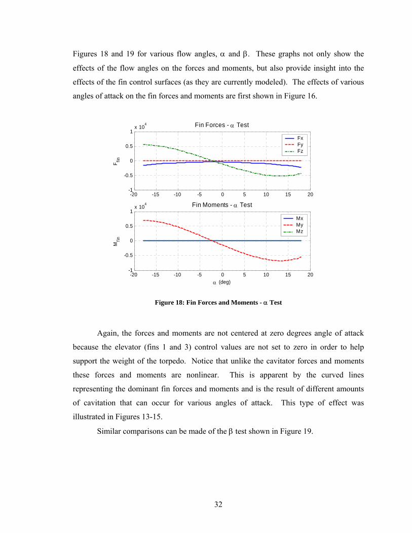
Figures 18 and 19 for various flow angles, α and β. These graphs not only show the

effects of the flow angles on the forces and moments, but also provide insight into the

effects of the fin control surfaces (as they are currently modeled). The effects of various

angles of attack on the fin forces and moments are first shown in Figure 16.

-20 -15 -10 -5 0 5 10 15 20-1

-0.5

0

0.5

1x 10

4

F fin

Fin Forces - α Test

-20 -15 -10 -5 0 5 10 15 20-1

-0.5

0

0.5

1x 10

4

α (deg)

Mfin

Fin Moments - α Test

FxFyFz

MxMyMz

Figure 18: Fin Forces and Moments - α Test

Again, the forces and moments are not centered at zero degrees angle of attack

because the elevator (fins 1 and 3) control values are not set to zero in order to help

support the weight of the torpedo. Notice that unlike the cavitator forces and moments

these forces and moments are nonlinear. This is apparent by the curved lines

representing the dominant fin forces and moments and is the result of different amounts

of cavitation that can occur for various angles of attack. This type of effect was

illustrated in Figures 13-15.

Similar comparisons can be made of the β test shown in Figure 19.

32

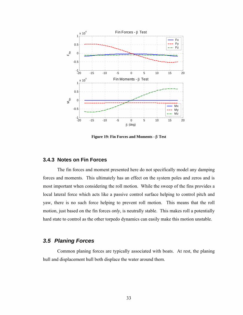
-20 -15 -10 -5 0 5 10 15 20-1

-0.5

0

0.5

1x 10

4

F fin

Fin Forces - β Test

-20 -15 -10 -5 0 5 10 15 20-1

-0.5

0

0.5

1x 10

4

β (deg)

Mfin

Fin Moments - β Test

FxFyFz

MxMyMz

Figure 19: Fin Forces and Moments - β Test

3.4.3 Notes on Fin Forces

The fin forces and moment presented here do not specifically model any damping

forces and moments. This ultimately has an effect on the system poles and zeros and is

most important when considering the roll motion. While the sweep of the fins provides a

local lateral force which acts like a passive control surface helping to control pitch and

yaw, there is no such force helping to prevent roll motion. This means that the roll

motion, just based on the fin forces only, is neutrally stable. This makes roll a potentially

hard state to control as the other torpedo dynamics can easily make this motion unstable.

3.5 Planing Forces

Common planing forces are typically associated with boats. At rest, the planing

hull and displacement hull both displace the water around them.

33

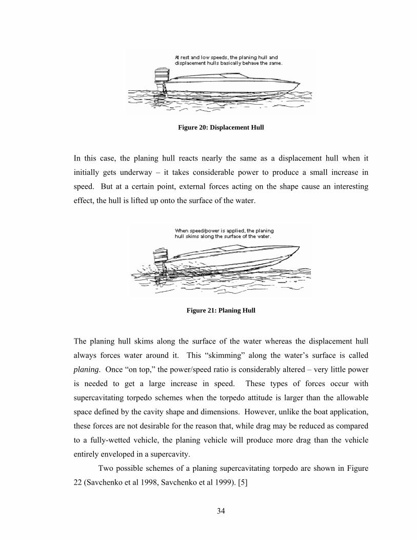
Figure 20: Displacement Hull

In this case, the planing hull reacts nearly the same as a displacement hull when it

initially gets underway – it takes considerable power to produce a small increase in

speed. But at a certain point, external forces acting on the shape cause an interesting

effect, the hull is lifted up onto the surface of the water.

Figure 21: Planing Hull

The planing hull skims along the surface of the water whereas the displacement hull

always forces water around it. This “skimming” along the water’s surface is called

planing. Once “on top,” the power/speed ratio is considerably altered – very little power

is needed to get a large increase in speed. These types of forces occur with

supercavitating torpedo schemes when the torpedo attitude is larger than the allowable

space defined by the cavity shape and dimensions. However, unlike the boat application,

these forces are not desirable for the reason that, while drag may be reduced as compared

to a fully-wetted vehicle, the planing vehicle will produce more drag than the vehicle

entirely enveloped in a supercavity.

Two possible schemes of a planing supercavitating torpedo are shown in Figure

22 (Savchenko et al 1998, Savchenko et al 1999). [5]

34

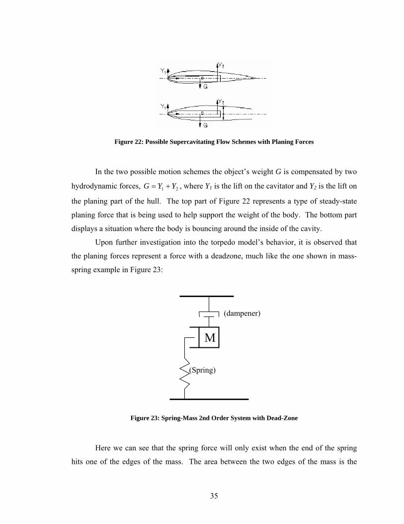
Figure 22: Possible Supercavitating Flow Schemes with Planing Forces

In the two possible motion schemes the object’s weight G is compensated by two

hydrodynamic forces, 21 YYG += , where Y1 is the lift on the cavitator and Y2 is the lift on

the planing part of the hull. The top part of Figure 22 represents a type of steady-state

planing force that is being used to help support the weight of the body. The bottom part

displays a situation where the body is bouncing around the inside of the cavity.

Upon further investigation into the torpedo model’s behavior, it is observed that

the planing forces represent a force with a deadzone, much like the one shown in mass-

spring example in Figure 23:

(dampener)

M

(Spring)

Figure 23: Spring-Mass 2nd Order System with Dead-Zone

Here we can see that the spring force will only exist when the end of the spring

hits one of the edges of the mass. The area between the two edges of the mass is the

35

deadzone. This deadzone is similar to the inside of the cavity and the mass edges are

similar to the cavity boundaries (dimensions).

What this means is that a linearized system would not be representative of all the

possible dynamics. In other words, when planing forces exist, the torpedo is actually a

different system. For this spring mass example shown above, there would have to be

three linear models to represent the three systems: (1) when the spring is not hitting the

edge of the mass, (2) when the spring hits the bottom edge, and (3) when the spring hits

the top edge. A similar process must be applied to the torpedo model for when the

torpedo is planing and when it is not. There are numerous studies in how to handle these

types of nonlinearities in control law design if one decides that it is possible to control the

torpedo (given the very high bandwidth) in the presence of strong and frequent planing

forces.

Planing of a slender afterbody on a supercavitating boundary also distorts the flow

(Logvinovich, 1980). The pressure increase on the wetted portion of the section is

associated with the deflection of the streamlines toward the cavity region. This results in

a jet of fluid into the cavity on each side of the body similar to the spray jet observed

along planing hulls. Both types of secondary flows – due to the fins and to the afterbody

planing – have been ignored in the current investigation, although the theory used to

estimate the afterbody planing forces accounts for the lowest-order effect of the spray jet.

[1]

Planing forces acting on the blast tube used for propulsion is assumed to be

negligible for reasons that this aft part of the cavity will, in reality, have a large void

fraction and so the hydrodynamic forces acting on the blast tube would be small. Further

studies have been done on the afterbody cavity dynamics by Travis Schauer at the

University of Minnesota and more information regarding these void fractions can be seen

in his Master’s thesis.

The importance of cavity distortion in high turn rates is apparent in Figure 24

which represents results for an extreme turn (in this case, a 5-g turn, which is probably

impractical, but is illustrative for the cavity-body interactions important to the dynamics).

36

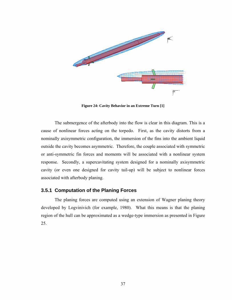
Z X

Y

X

Y

Z

Figure 24: Cavity Behavior in an Extreme Turn [1]

The submergence of the afterbody into the flow is clear in this diagram. This is a

cause of nonlinear forces acting on the torpedo. First, as the cavity distorts from a

nominally axisymmetric configuration, the immersion of the fins into the ambient liquid

outside the cavity becomes asymmetric. Therefore, the couple associated with symmetric

or anti-symmetric fin forces and moments will be associated with a nonlinear system

response. Secondly, a supercavitating system designed for a nominally axisymmetric

cavity (or even one designed for cavity tail-up) will be subject to nonlinear forces

associated with afterbody planing.

3.5.1 Computation of the Planing Forces

The planing forces are computed using an extension of Wagner planing theory

developed by Logvinivich (for example, 1980). What this means is that the planing

region of the hull can be approximated as a wedge-type immersion as presented in Figure

25.

37

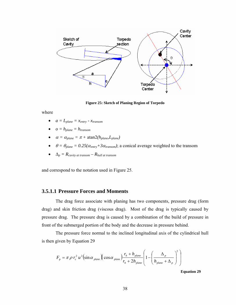
Figure 25: Sketch of Planing Region of Torpedo

where

• a = Lplane = xentry - xtransom

• o = hplane = htransom

• α = αplane = π + atan2(hplane,Lplane)

• θ = θplane = 0.25(αentry+3αtransom); a conical average weighted to the transom

• Δp = Rcavity at transom – Rhull at transom

and correspond to the notation used in Figure 25.

3.5.1.1 Pressure Forces and Moments

The drag force associate with planing has two components, pressure drag (form

drag) and skin friction drag (viscous drag). Most of the drag is typically caused by

pressure drag. The pressure drag is caused by a combination of the build of pressure in

front of the submerged portion of the body and the decrease in pressure behind.

The pressure force normal to the inclined longitudinal axis of the cylindrical hull

is then given by Equation 29

( )( ) ⎟⎟

⎠

⎞

⎜⎜

⎝

⎛

⎟⎟⎠

⎞⎜⎜⎝

⎛

Δ+

Δ−

+

+=

2

22cp 1

2cossin

pplane

p

planeh

planehplaneplane hhr

hrurF ααρπ

Equation 29

38

where rh is the hull radius (assumed to be constant over the planing region), rc, αplane, and

are (respectively) the cavity radius (at transom), the angle of attack between the

longitudinal axes of the body and the cavity, and the difference between the cavity and

hull radii (all averaged along the planing region); and is the immersion depth at the

transom measured normal to the cavity centerline.

Δ

0h

Similarly, the moment of pressure forces about the transom can be expressed as

pplane

plane

plane

plane

hh

hrhr

urMΔ++

+=

2

h

hplane

222cp 2

cos αρπ Equation 30

3.5.1.2 Skin Friction Forces

The skin friction forces, caused by the viscosity of water, were computed using

the following set of equations [1]:

71

031.0

2

⎟⎟⎠

⎞⎜⎜⎝

⎛=

Δ=

Δ=

νplane

d

planeph

s

p

planec

uLC

hr

u

hu

( )[ ]+−+Δ

= cccplane

phw uuurS arctan1

tan4 2

α

( )[ ]221

212

3

1arcsintan2 ssss

planep

h uuuur

−+−Δ α

dwplanef CSuF αρ 2221 cos= Equation 31

39

where u is the forward velocity state and the moments are assumed to be negligible.

3.5.1.3 Added Mass and Impact Forces

The extra terms that are now added to the planing force computation is the

unsteady force which is proportional to the acceleration and the impact force which is

proportional to the impact speed and the speed of sound in water. The impact force is

important for the case when the hull of the torpedo hits the surface of the cavity.

The generic forces due to acceleration and impact are represented as

Equation 32 amCF addedaonaccelerati =

Equation 33 pwimpactiimpact VACmCF =

where C is the speed of sound in water, a and V are the acceleration and velocities of the

center of mass of the wetted wedge (computed using the norm of the q and r components

of the state-space derivative and state-space, respectively), Apw is the projected area of the

surface area of the wetted wedge, and Ca and Ci are coefficients for the acceleration and

impact forces respectively and are yet to be determined through CFD analysis. Currently,

an upper limit based on a fully wetted cylindrical body, the values of Ca and Ci are 1 and

½, respectively. madded and mimpact are related to the geometry. For a noncavitating sphere

the added mass is equal to half the displaced water, but for a cavitating body, there is no

such compact result. For now, a crude approximation is to set the added mass equal to the

cavity volume and the impact mass to the mass of the displaced water by the impacting

hull.

3.5.1.4 Total Planing Forces and Moments

The total planing forces and moments then become

40

( )( ) ⎥

⎥⎥

⎦

⎤

⎢⎢⎢

⎣

⎡

++++−=

planeimpactonacceleratip

planeimpactonacceleratip

f

plane

FFFFFF

FF

θθ

sincos Equation 34

⎥⎥⎥

⎦

⎤

⎢⎢⎢

⎣

⎡×+

⎥⎥⎥

⎦

⎤

⎢⎢⎢

⎣

⎡

−=

00

cossin0 ,wedgecg

plane

cp

cpplane

xF

MMM

θθ Equation 35

3.5.2 Effects of Planing

The magnitude of the forces are large (on the order of 6000 N!) and occur at

dominating frequencies11 of about 10 Hz, 25 Hz, and 50 Hz as seen in Figure 26. Keep

in mind that these frequencies and forces are specific to the torpedo geometry described

above as well as the flight condition and may be different for other torpedo models. Due

to the large forces and the high frequency (with dominant modes as high as 50 Hz) of

these forces, not to mention the large increase in drag associated with planing, planing

forces are considered undesirable and are not required for the overall stability of the

torpedo as long as there are other control surfaces such as fins to help support the weight.

In addition, the model becomes a switching model with the cavity dimensions at

the transom of the torpedo representing the dead-zone region. Since the dominant

frequencies of the planing forces are about 10 Hz, 25 Hz, and 50 Hz it would take

significant control effort as well as very fast and expensive actuators and sensors to

actively control the torpedo at this high of a bandwidth. This is why this thesis treats the

planing forces as a general disturbance (which is a function of the states) in the nonlinear

model which means that these forces are not used to compute the linear model used for

control law design. Rather, they will be used to help specify the constraints on the

turning accelerations for the horizontal trajectories considered in order to minimize the

allowable planing forces. In other words, allowable trajectories will be based on the

steady-state turn rate required to produce planing forces. 11 These frequencies are based on the original model developed by Anteon for fin and planing force supported, straight-and-level flight at a speed of 77 m/s.

41

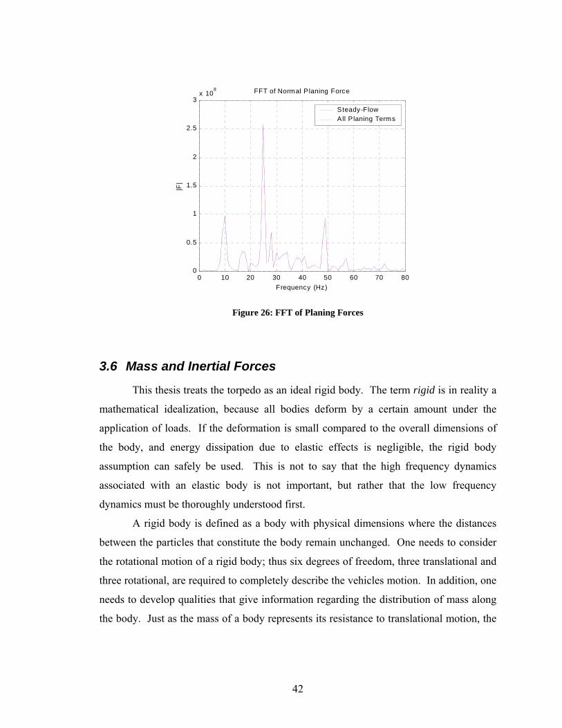
0 10 20 30 40 50 60 70 80

0

0.5

1

1.5

2

2.5

3x 10

8

Frequency (Hz)

|F|

FFT of Normal Planing Force

Steady-Flow A ll P laning Terms

Figure 26: FFT of Planing Forces

3.6 Mass and Inertial Forces

This thesis treats the torpedo as an ideal rigid body. The term rigid is in reality a

mathematical idealization, because all bodies deform by a certain amount under the

application of loads. If the deformation is small compared to the overall dimensions of

the body, and energy dissipation due to elastic effects is negligible, the rigid body

assumption can safely be used. This is not to say that the high frequency dynamics

associated with an elastic body is not important, but rather that the low frequency

dynamics must be thoroughly understood first.

A rigid body is defined as a body with physical dimensions where the distances

between the particles that constitute the body remain unchanged. One needs to consider

the rotational motion of a rigid body; thus six degrees of freedom, three translational and

three rotational, are required to completely describe the vehicles motion. In addition, one

needs to develop qualities that give information regarding the distribution of mass along

the body. Just as the mass of a body represents its resistance to translational motion, the

42

distribution of the mass about a certain axis represents the body’s resistance to rotational

motion about that axis.

3.6.1 Center of Mass

A rigid body can be considered as a collection of particles in which the number of

particles approaches infinity and in which the distances between the individual masses

remain the same. As N approaches infinity, each particle can be treated as a differential

mass element dm and the mass of the body is computed as an integral over the body

dimensions

∫=body

dmm

where the nominal mass is set at 175.7 Kg for this investigation.

The location of the center of mass can then be defined as

∫ ⋅=body

G dmrm

r 1

where r is the vector from the origin to the differential element dm. Since the torpedo is

symmetric about the ξ-axis, the only nonzero element of rG is the ξ-component and will

be defined as xcg and is measured in units aft of the cavitator.

The center of mass is a very important quantity, as its use simplifies the analysis

of bodies considerably. One has to perform the integrations above in order to find the

center of mass. These integrals in general are triple integrals, but in order to simplify the

problem the geometry of the torpedo is considered and uniform density is assumed. As is

shown in Figure 27, the torpedo geometry can be broken into four main sections: (1) the

cavitator/pivot joints, (2) nose cone, (3) body cylinder, and (4) the blast tube. Since it is

reasonable to consider most of the mass to be contained in the nose cone and the

cylindrical body, we just need to know the simple geometry of those sections.

43

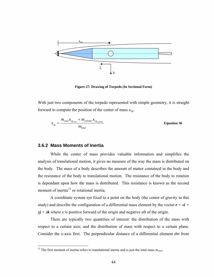
xcg

ξ h

Figure 27: Drawing of Torpedo (In Sectional Form)

With just two components of the torpedo represented with simple geometry, it is straight

forward to compute the position of the center of mass xcg.

total

cgcylindercgconecg m

xmxmx cylindercone

+= Equation 36

3.6.2 Mass Moments of Inertia

While the center of mass provides valuable information and simplifies the

analysis of translational motion, it gives no measure of the way the mass is distributed on

the body. The mass of a body describes the amount of matter contained in the body and

the resistance of the body to translational motion. The resistance of the body to rotation

is dependant upon how the mass is distributed. This resistance is known as the second

moment of inertia12 or rotational inertia.

A coordinate system xyz fixed to a point on the body (the center of gravity in this

study) and describe the configuration of a differential mass element by the vector r = xi +

yj + zk where x is positive forward of the origin and negative aft of the origin.

There are typically two quantities of interest: the distribution of the mass with

respect to a certain axis; and the distribution of mass with respect to a certain plane.

Consider the x-axis first. The perpendicular distance of a differential element dm from

12 The first moment of inertia refers to translational inertia and is just the total mass mtotal.

44

the x-axis is 22 zyRx += . The mass moment of inertia about the x-axis is then

computed as

dmzydmRJbodybody

xxx ⋅+=⋅= ∫∫ 222 Equation 37

In a similar fashion, the mass moments of inertia about the y and z axes are defined as

Equation 38 dmzxdmRJbodybody

yyy ⋅+=⋅= ∫∫ 222

Equation 39 dmyxdmRJbodybody

zzz ⋅+=⋅= ∫∫ 222

One quick observation is that the mass moment of inertia of a body about a

certain axis becomes larger as the axis is selected further away from the body. This is an

indication that mass moments of inertia will be useful in describing the rotational motion

of a body.

Consider the distribution of the mass with respect to the xy, xz, and yz planes;

these produce the products of inertia.

Equation 40 ∫ ⋅=body

xy dmxyJ

Equation 41 ∫ ⋅=body

yz dmyzJ

Equation 42 ∫ ⋅=body

xz dmxzJ

It is clear that Jxy=Jyx, and so forth. In general, the products of inertia do not contribute

too much to the physical description of the mass distribution, unless there are certain

symmetry properties with respect to the coordinate axes. Since the fins are oriented in

the cross formation and line up with the principal axes, the products of inertia are zero

unless an origin is chosen to be something other than the center of mass.

The moments and products of inertia form the so called inertia matrix, denoted by

[J] and is defined as

45

Equation 43 [ ]⎥⎥⎥

⎦

⎤

⎢⎢⎢

⎣

⎡

−−−−−−

=

zzyzxz

yzyyxy

xzxyxx

JJJJJJJJJ

J

The diagonal elements of [J] are the principal moments of inertia and they are all positive

quantities, each obtained by integration of a positive integrand.

The mass, center of mass, and the inertia matrix of a rigid body specify what are

called the internal properties is the body completely. For an elastic body, one needs to

know measures of the resistance of the body to deformation, in addition to the internal

properties.

To compute the components of the inertia matrix, the simple torpedo geometry

can be taken advantage of again by use of the parallel axis theorem. In other words, the

moments of inertia are computed for the cone and the cylinder separately taking into

consideration the distance from the section’s center of gravity to the origin and then

performing the following calculation (parallel axis theorem).

Equation 44 ⎥⎥⎥

⎦

⎤

⎢⎢⎢

⎣

⎡

+−−−+−−−+

+=22

22

22

yxzyzx

zyzxyx

zxyxzy

iGB

dddddddddddddddddd

mJJii

where JG are the moments of inertia of the individual section, mi is the mass of the

section, and dx, dy, and dz represent the distances to the origin in the ξ-, η-, and h-axes.

The total inertia is then computed by summing the two sections of inertia.

3.7 Putting it all Together

A variety of methods exist for writing equations of motion (EOM) for dynamical

systems. One of the most common is the Newton-Euler formulation. From a historical

perspective, Newton developed his laws for the motion of rigid bodies, even though we

first study them within the context of particles. Defining the inertia force acting on the

body as –macg, Newton’s second law can be described as the inertia force being equal and

opposite to the applied forces. The law governing rotational motion was formally stated

by Euler in 1775. The law states that the rate of change of the angular momentum about

46

the center of mass of a rigid body is equal to the sum of all applied moments about the

center of mass. [8]

Using this methodology, the system dynamics about the center of gravity in an

inertial coordinate system are computed as shown in the following matrix notation form

of the EOM.

cgcgcgcgcg M

FJ

mIJ

mI⎥⎦

⎤⎢⎣

⎡+⎥

⎦

⎤⎢⎣

⎡⎥⎦

⎤⎢⎣

⎡⎥⎦

⎤⎢⎣

⎡−

−=⎥

⎦

⎤⎢⎣

⎡⎥⎦

⎤⎢⎣

⎡

∑∑××

ων

ωω

ων

00

~00~

00 3333

&&

Equation 45

where

[ ][ ]T

T

rqp

wvu

=

=

ω

ν

are the linear and angular velocity vectors, respectively, F and M are the external forces

and moments acting about the center of gravity, and the tilde (~) character is used to

represent the cross product of a vector in matrix form. The inertia about the center of

gravity is defined as Jcg.

The tilde character is used as follows:

[ ]⎥⎥⎥

⎦

⎤

⎢⎢⎢

⎣

⎡

−−

−=→=

00

0~

abac

bccba T κκ

and is the same as using the cross product as is illustrated below.

⎥⎥⎥

⎦

⎤

⎢⎢⎢

⎣

⎡

⎥⎥⎥

⎦

⎤

⎢⎢⎢

⎣

⎡

−−

−=

⎥⎥⎥

⎦

⎤

⎢⎢⎢

⎣

⎡×⎥⎥⎥

⎦

⎤

⎢⎢⎢

⎣

⎡

nml

abac

bc

nml

cba

00

0

Note that the tilde matrix representation is a skew-symmetric matrix.

It is often convenient to write the EOM in short-hand notation with the help of the

tilde operation described above. Defining a mass matrix, M, and angular rate matrix, Ω,

such that

47

⎥⎦

⎤⎢⎣

⎡−

−=Ω

⎥⎦

⎤⎢⎣

⎡= ×

ωω

~00~

0033

cgJmI

M

The equations of motion about the center of gravity (Equation 45) are then written as

cgcgcg M

FMM ⎥

⎦

⎤⎢⎣

⎡+⎥

⎦

⎤⎢⎣

⎡Ω=⎥

⎦

⎤⎢⎣

⎡

∑∑

ων

ων&&

Equation 46

3.7.1 EOM about an Arbitrary Point

If it is desired to compute the EOM about an arbitrary point other than the center

of mass (such as the cavitator pivot point as is considered by Anteon), appropriate

transformations must be added to these system equations of motion. If a vector defining

the distance to the arbitrary point from the center of mass is defined as

[ ]Tzyx rrrr =

where distances are positive in the positive directions of the coordinate system, the

velocity components of the system are transformed to the new coordinate system. In

other words, we substitute the velocity components about the center of gravity with the

transformed values such that

⎥⎦

⎤⎢⎣

⎡=⎥

⎦

⎤⎢⎣

⎡⎥⎦

⎤⎢⎣

⎡=⎥

⎦

⎤⎢⎣

⎡

×

×

ων

ων

ων

RIrI

cg 33

33

0

~ Equation 47

where R is the origin transformation matrix. Substituting and making sure that the forces

and moments are in the correct reference frames, the EOM become

cg

TTT

MF

RMRRMRR ⎥⎦

⎤⎢⎣

⎡+⎥

⎦

⎤⎢⎣

⎡Ω=⎥

⎦

⎤⎢⎣

⎡

∑∑

ων

ων&&

Equation 48

48

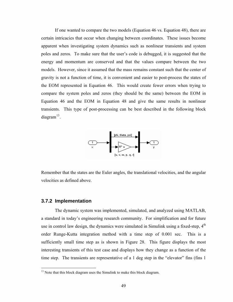
If one wanted to compare the two models (Equation 46 vs. Equation 48), there are

certain intricacies that occur when changing between coordinates. These issues become

apparent when investigating system dynamics such as nonlinear transients and system

poles and zeros. To make sure that the user’s code is debugged, it is suggested that the

energy and momentum are conserved and that the values compare between the two

models. However, since it assumed that the mass remains constant such that the center of

gravity is not a function of time, it is convenient and easier to post-process the states of

the EOM represented in Equation 46. This would create fewer errors when trying to

compare the system poles and zeros (they should be the same) between the EOM in

Equation 46 and the EOM in Equation 48 and give the same results in nonlinear

transients. This type of post-processing can be best described in the following block

diagram13.

Remember that the states are the Euler angles, the translational velocities, and the angular

velocities as defined above.

3.7.2 Implementation

The dynamic system was implemented, simulated, and analyzed using MATLAB,

a standard in today’s engineering research community. For simplification and for future

use in control law design, the dynamics were simulated in Simulink using a fixed-step, 4th

order Runge-Kutta integration method with a time step of 0.001 sec. This is a

sufficiently small time step as is shown in Figure 28. This figure displays the most

interesting transients of this test case and displays how they change as a function of the

time step. The transients are representative of a 1 deg step in the “elevator” fins (fins 1

13 Note that this block diagram uses the Simulink to make this block diagram.

49

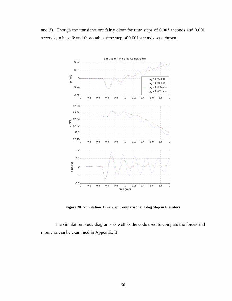
and 3). Though the transients are fairly close for time steps of 0.005 seconds and 0.001

seconds, to be safe and thorough, a time step of 0.001 seconds was chosen.

0 0.2 0.4 0.6 0.8 1 1.2 1.4 1.6 1.8 2-0.02

-0.01

0

0.01

0.02

θ (ra

d)

Simulation Time Step Comparisons

0 0.2 0.4 0.6 0.8 1 1.2 1.4 1.6 1.8 282.18

82.2

82.22

82.24

82.26

82.28

u (m

/s)

0 0.2 0.4 0.6 0.8 1 1.2 1.4 1.6 1.8 2-0.2

-0.1

0

0.1

0.2

q (ra

d/s)

time (sec)

Δ t = 0.05 secΔ t = 0.01 secΔ t = 0.005 secΔ t = 0.001 sec

Figure 28: Simulation Time Step Comparisons: 1 deg Step in Elevators

The simulation block diagrams as well as the code used to compute the forces and

moments can be examined in Appendix B.

50

4 Linearization A classical dilemma in modeling physical systems is the trade-off between model

accuracy and tractability. While sophisticated models might provide accurate

descriptions of system behavior, the resulting analysis can be considerably more

complicated. Simpler models, on the other hand, may make analysis easier and offer

more insight, but might neglect important system behaviors. The required fidelity of a

model depends on the intended utility. For example, one may use a very simplified

model for the sake of control design, but then use a sophisticated model to simulate the

overall control system.

One instance where this dilemma manifests itself is the use of linear versus

nonlinear models. Nonlinearities occur in most physical systems. Simple examples

include saturations, rate limiters, dead-zones, and backlash. Further examples include

inherently nonlinear behavior of systems such as chemical process plants, aircraft, and

the torpedo model under inspection. However, methods for analysis and control design

are considerably more available and developed for linear systems than nonlinear systems.

One approach is to directly address the nonlinear behavior of such systems, and

nonlinear control design remains a topic of active research. An alternative method is to

linearize the system dynamics; i.e. to approximate the nonlinear model by a linear one.

Some immediate consequences are that (1) the linear model can only give a local

description of the system behavior and (2) some of the intricacies of the system behavior

may be completely neglected – even locally. In some cases, these consequences are

tolerable, and one may then employ methods for linear systems.

Recall that the main reason for continuing to understand and further the

development of the torpedo’s dynamic model (rather than diving into control law design)

is because there is an issue with the previous model developed by Kirschner et. al; that is

that the stable nonlinear transients did not match the unstable linear description of the

model. This means that it is probable that some of the model intricacies were not being

captured by the linearization process. The following provides detailed description of the

process of linearization and situations when this process fails in a general form.

51

4.1 General Linearization Procedures and Information

The goal of linearization is to provide insight into nonlinear system behavior

about an equilibrium point and to give the engineer some useful tools for attacking

certain classes of nonlinear problems. Many systems with mild, sufficiently smooth

nonlinearities can be treated by using a linear approximate model, obtained by linearizing

about a known nominal solution or operating point. Most control design is based on

behavior in the vicinity of an “operating point.” Many aircraft, rocket, and spacecraft

control systems have been successfully designed using linear behavior in the

neighborhood of a nominal trajectory.

Consider the general time-invariant nonlinear state variable mode of Equations 49

and 50:

Equation 49 ( Δ= ,xfx& )

) Equation 50 ( Δ= ,xgy

where x is the state vector, Δ is the input vector, and y is the output vector. Suppose that

a nominal solution xn, Δn, and yn, such as an equilibrium point, is known. The difference

between the nominal vector functions and some slightly perturbed functions x, Δ, and y

can be defined by

n

n

n

yyy

xxx

−=Δ−Δ=Δ

−=

δδδ

Then Equations 49 and 50 can be written as

( )Δ+Δ+=+ δδδ nnn xxfxx ,&&

( ) tohfxxfUxf

nnnn .., +Δ⎥⎦

⎤⎢⎣⎡Δ∂∂

+⎥⎦⎤

⎢⎣⎡∂∂

+= δδ Equation 51

( )UUxxgyy nnn δδδ ++=+ ,

52

( ) tohgxxgUyg

nnnn .., +Δ⎥⎦

⎤⎢⎣⎡Δ∂∂

+⎥⎦⎤

⎢⎣⎡∂∂

+= δδ Equation 52

where []n means that the derivatives, the Jacobians, are evaluated on the nominal

solutions. Since the nominal solutions satisfy Equations 49 and 50, the first terms in the

preceding Taylor’s series expansion cancel.

One other condition must also hold. For sufficiently small xδ , Δδ , and

yδ perturbations, the higher-order terms must approach zero as x approaches xn, that is:

0...

suplim0

=≥→ x

tohtxx n

Equation 53

Since these higher-order terms can be neglected, this leaves the linear time-invarient

(LTI) equations

Δ⎥⎦⎤

⎢⎣⎡Δ∂∂

+⎥⎦⎤

⎢⎣⎡∂∂

=

Δ⎥⎦⎤

⎢⎣⎡Δ∂∂

+⎥⎦⎤

⎢⎣⎡∂∂

=

δδδ

δδδ

nn

nn

gxxgy

fxxfx&

Equation 54

which is equal to

Equation 55 Δ+=Δ+=

DCxyBAxx&

when (xn, Δn) is equal to (0,0) and the matrices A, B, C, and D are the respective

Jacobians.

4.1.1 Limitations of Linearization

There are a couple of nonlinearities that do not lend themselves to linearization-

based analysis. Consider the system

Equation 56 )(Δ+= BNAxx&

This system represents linear dynamics where the input u first passes through a

nonlinearity, N. Some common nonlinearities are:

53

saturation14:

Equation 57 ⎪⎩

⎪⎨

⎧

−≤Δ−≤Δ≤−Δ

≥Δ=Δ

1111

11)(N

deadzone:

Equation 58 ⎪⎩

⎪⎨

⎧

−≤Δ+Δ≤Δ≤−

≥Δ−Δ=Δ

11110

11)(N

and relay:

Equation 59 ⎩⎨⎧

<Δ−>Δ

=Δ0101

)(N

Other nonlinearities include backlash and hysteresis. All of these nonlinearities result in

a failure in linearization-based analysis because the linearization completely removes the

intricacies that the nonlinearities cause. i.e. N(Δ) is not differentiable (the slope is not

smooth).

5 Flight Envelope In order to define the flight envelope, the constant cavitation number of 0.029

must be considered. Given the definition of σ in Equation 1 the velocity needed to

maintain this cavitation number can be solved providing we know something about the

freestream pressure, cavity pressure, and water density. If the freestream pressure is

assumed to be about 101325 Pa and the cavity pressure is assumed to be water vapor

pressure at a temperature of 41o F (871.928 Pa) and a density of 1024 kg/m3, the velocity

required to maintain the cavitation number of 0.029 would be about 82.25 m/s. Since the

temperature of the water and operating depth (assumed to be about ten meters) greatly

affect the density and pressure, the velocity value is allowed to vary by 10% of the

nominal value. This gives a velocity operating range of about V = [74,90] m/s. Note that

14 Note that from the definition of Equation 51 that this is only true when the Δ has hit a saturation point.

54

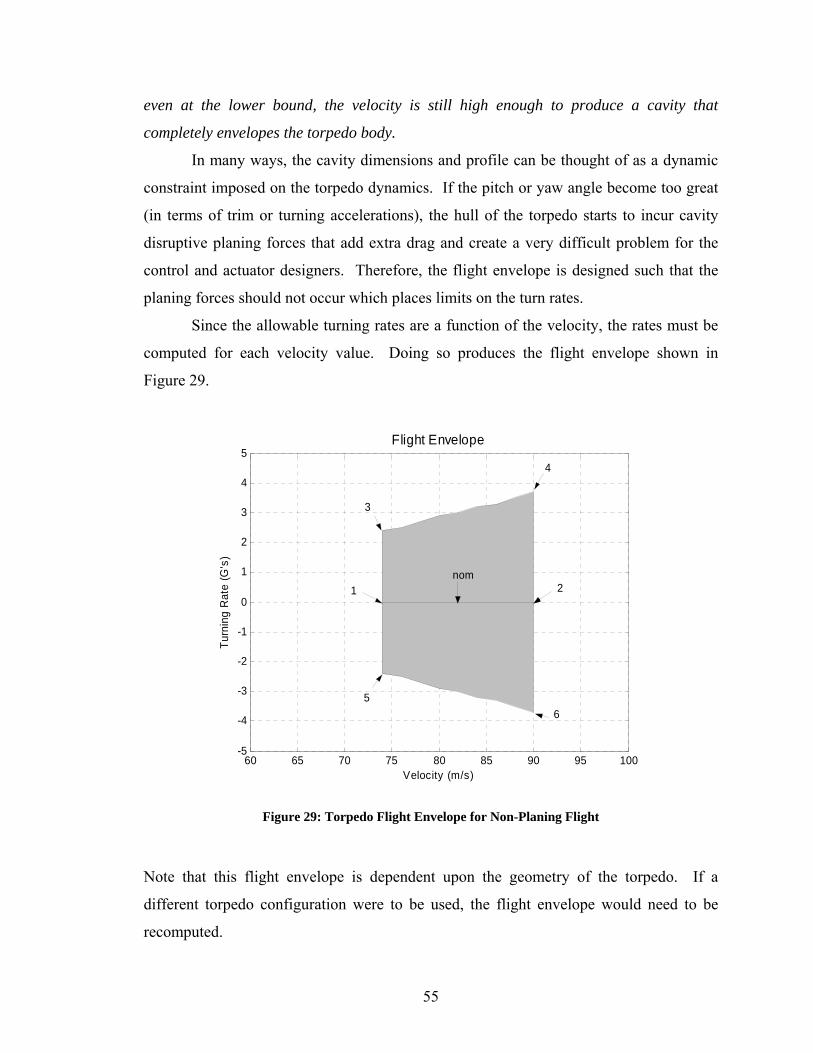
even at the lower bound, the velocity is still high enough to produce a cavity that

completely envelopes the torpedo body.

In many ways, the cavity dimensions and profile can be thought of as a dynamic

constraint imposed on the torpedo dynamics. If the pitch or yaw angle become too great

(in terms of trim or turning accelerations), the hull of the torpedo starts to incur cavity

disruptive planing forces that add extra drag and create a very difficult problem for the

control and actuator designers. Therefore, the flight envelope is designed such that the

planing forces should not occur which places limits on the turn rates.

Since the allowable turning rates are a function of the velocity, the rates must be

computed for each velocity value. Doing so produces the flight envelope shown in

Figure 29.

60 65 70 75 80 85 90 95 100-5

-4

-3

-2

-1

0

1

2

3

4

5

Velocity (m/s)

Turn

ing

Rat

e (G

's)

Flight Envelope

nom

3

4

1 2

6 5

Figure 29: Torpedo Flight Envelope for Non-Planing Flight

Note that this flight envelope is dependent upon the geometry of the torpedo. If a

different torpedo configuration were to be used, the flight envelope would need to be

recomputed.

55

In order to fully understand the torpedo model, several linear models of the open-

loop torpedo model for various trim conditions should be computed and analyzed. In

order to get a representation of the full flight envelope, a linear model should be taken for

the nominal model (V = 82.25 m/s, turning acceleration = 0 g’s) as well as six other trim

conditions indicated in Figure 29. What’s more important is that since the controller can

typically only be designed with one nominal model, it is important to test the closed-loop

system with all trim conditions in order to make sure that the controller performs as

intended for all possible flight conditions.

6 Stability and System Poles One of the most important characteristics of both nonlinear and linear systems is

its stability. For completeness and in order to better understand the analysis of the

torpedo, the definitions of stability and some of the tools used to determine system

stability are presented below.

Consider the state equation written in Equation 49. For the continuous-time case

with zero input

)0,(xfx =&

with the origin defined at the equilibrium trim condition, the following apply.

Definition 1

The origin is a stable equilibrium point if there exists an ε > 0 and a δ(ε,t0) > 0,

such that if )( 0tx < δ, then the resultant motion x(t) satisfies )(tx < ε for all t >

t0.

This definition of stability is sometimes called stability in the sense of Lyapunov,

abbreviated as stable i.s.L. If a system possesses this type of stability, then it is ensured

56

that the state can be kept within ε, in norm, of the origin by restricting the initial

perturbation to be less than δ, in norm. Note that it is necessarily true that εδ ≤ .

Definition 2

The origin is an asymptotically stable stable equilibrium point if (a) it is stable,

and if in addition, (b) there exists a number δ(t0) > 0 such that whenever

( )00 )( ttx δ< the resultant motion satisfies ( ) 0lim =∞→

txt

.

The following is a standard analysis result based on Definition 2. The equilibrium

point xn equal to x0 is asymptotically stable if all of the eigenvalues (poles15) of the

Jacobian ( )

j

i

xxf∂

Δ∂ , (the state-space A-matrix) have negative real parts. It is unstable if A

has an eigenvalue with a positive real part. If one or more of the eigenvalues are on the

jϖ axis and all others are in the left-half plane, no conclusions about stability can be

drawn from the linear model. Whether the actual behavior of the system is divergent or

convergent will then depend upon the higher-order terms in the Taylor’s Series

expansion. Thus, except for the borderline jϖ axis case, this result states that the

linearization can provide sufficient conditions for stability of the nonlinear system in a

neighborhood of an equilibrium point.

When nonzero inputs Δ(t) are considered, additional types of stability are often

used.

Definition 3 (Bounded input, bounded output stability)

Let u be a bounded input with Km as the least upper bound. If there exists a scalar

α such that for every t, the output satisfies mKy α≤ , then the system is bounded

input, bounded output stable, abbreviated as BIBO stable.

15 When the system equations are simultaneous linear ordinary differential equations (ODEs), the transfer function that results will be a ratio of polynomials; that is, ( ) ( ) ( )sasbsH = . If we assume that b and a have no common factors (as is usually the case), then values of s such that a(s)=0 will represent points where H(s) is infinity. These s-values are called poles of H(s). Values of s such that b(s)=0 are points where H(s)=0, and the corresponding s-locations are called zeros.

57

Some useful tools to analyze BIBO stability and full nonlinear stability include

phase-plane analysis and simulation.

6.1 Phase Plane Analysis

Phase-plane representations of nonlinear systems are used at various times to

analyze stability of a system because of the insight they provide. Although general

phase-plane analysis techniques exist, they are fully effective only for second-order

systems and are not pursued in detail here.

6.2 Simulation and Integration Schemes

Because of the lack of analytical solutions for nonlinear system equations,

simulation takes on a much greater significance. Many numerical integration schemes

will diverge if the integration step is too large for the frequency of the signal being

integrated. The major danger in applying fixed-step integration schemes to nonlinear

systems whose response frequencies may not be known in advance is that the numerical

algorithm instability may be falsely interpreted as a system instability. One approach

suggests that when a simulated response appears to be diverging, the simulation should

be retried using a smaller integration time-step.

Our simulations have been run with a time-step of 0.001 seconds with a 4th order

Runge-Kutta integration scheme. This time step appears to be sufficient, as was shown in

Figure 28, and allows the simulation to finish in a reasonable amount of time.

Note that there are other integration schemes that allow variable step sizes which

are adjusted based on the change in states, the errors associated with these methods can

be unquantifiable.

58

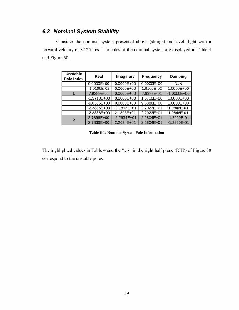
6.3 Nominal System Stability

Consider the nominal system presented above (straight-and-level flight with a

forward velocity of 82.25 m/s. The poles of the nominal system are displayed in Table 4

and Figure 30.

Unstable Pole Index Real Imaginary Frequency Damping

0.0000E+00 0.0000E+00 0.0000E+00 NaN-1.9100E-02 0.0000E+00 1.9100E-02 1.0000E+00

1 7.9389E-01 0.0000E+00 7.9389E-01 -1.0000E+00-1.5710E+00 0.0000E+00 1.5710E+00 1.0000E+00-9.6386E+00 0.0000E+00 9.6386E+00 1.0000E+00-2.3886E+00 -2.1893E+01 2.2023E+01 1.0846E-01-2.3886E+00 2.1893E+01 2.2023E+01 1.0846E-012.7866E+00 -2.2634E+01 2.2804E+01 -1.2220E-012.7866E+00 2.2634E+01 2.2804E+01 -1.2220E-012

Table 6-1: Nominal System Pole Information

The highlighted values in Table 4 and the “x’s” in the right half plane (RHP) of Figure 30

correspond to the unstable poles.

59

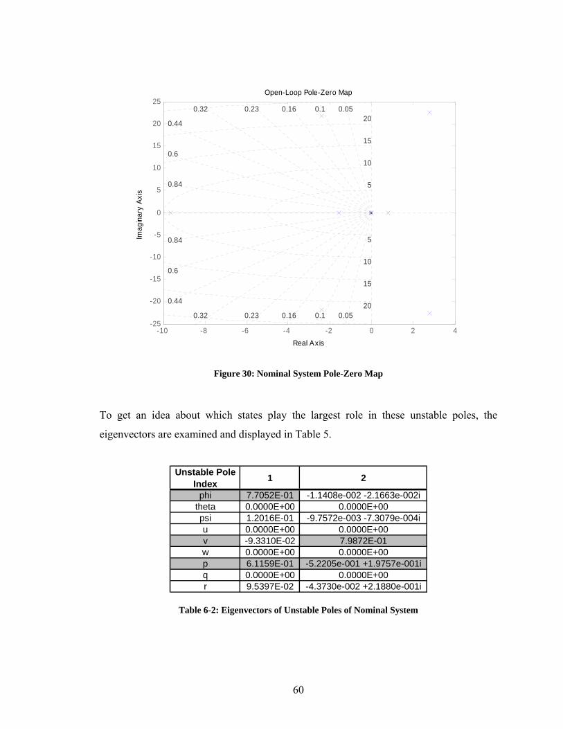
-10 -8 -6 -4 -2 0 2 4-25

-20

-15

-10

-5

0

5

10

15

20

25

0.05

0.84

0.050.10.160.230.32

0.44

0.6

0.84

0.10.160.230.32

0.44

0.6

5

10

15

20

20

5

10

15

Open-Loop Pole-Zero Map

Real Axis

Imag

inar

y Ax

is

Figure 30: Nominal System Pole-Zero Map

To get an idea about which states play the largest role in these unstable poles, the

eigenvectors are examined and displayed in Table 5.

Unstable Pole Index 1 2

phi 7.7052E-01 -1.1408e-002 -2.1663e-002itheta 0.0000E+00 0.0000E+00psi 1.2016E-01 -9.7572e-003 -7.3079e-004iu 0.0000E+00 0.0000E+00v -9.3310E-02 7.9872E-01w 0.0000E+00 0.0000E+00p 6.1159E-01 -5.2205e-001 +1.9757e-001iq 0.0000E+00 0.0000E+00r 9.5397E-02 -4.3730e-002 +2.1880e-001i

Table 6-2: Eigenvectors of Unstable Poles of Nominal System

60

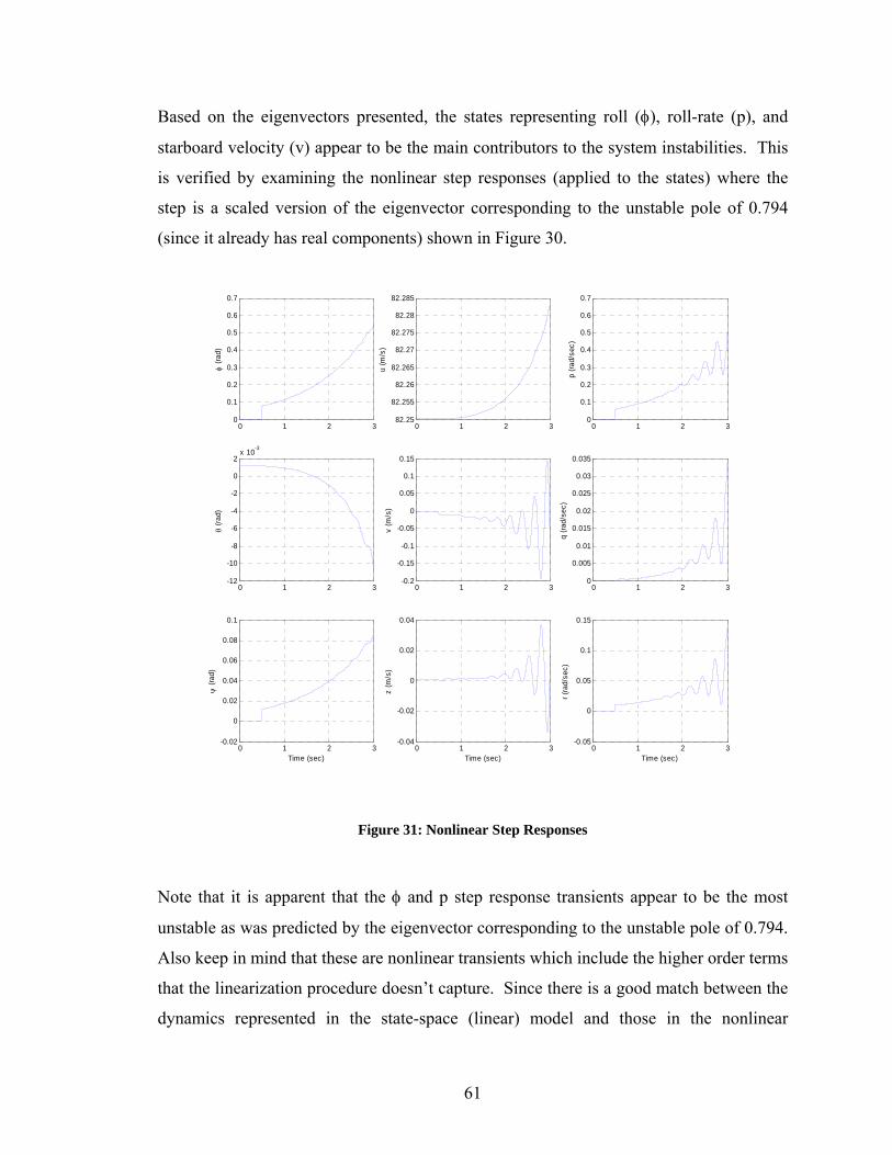
Based on the eigenvectors presented, the states representing roll (φ), roll-rate (p), and

starboard velocity (v) appear to be the main contributors to the system instabilities. This

is verified by examining the nonlinear step responses (applied to the states) where the

step is a scaled version of the eigenvector corresponding to the unstable pole of 0.794

(since it already has real components) shown in Figure 30.

0 1 2 30

0.1

0.2

0.3

0.4

0.5

0.6

0.7

φ (ra

d)

0 1 2 3-12

-10

-8

-6

-4

-2

0

2x 10-3

θ (ra

d)

0 1 2 3-0.02

0

0.02

0.04

0.06

0.08

0.1

ψ (r

ad)

Time (sec)

0 1 2 382.25

82.255

82.26

82.265

82.27

82.275

82.28

82.285

u (m

/s)

0 1 2 3-0.2

-0.15

-0.1

-0.05

0

0.05

0.1

0.15

v (m

/s)

0 1 2 3-0.04

-0.02

0

0.02

0.04

z (m

/s)

Time (sec)

0 1 2 30

0.1

0.2

0.3

0.4

0.5

0.6

0.7

p (ra

d/se

c)

0 1 2 30

0.005

0.01

0.015

0.02

0.025

0.03

0.035

q (ra

d/se

c)

0 1 2 3-0.05

0

0.05

0.1

0.15

r (ra

d/se

c)

Time (sec)

Figure 31: Nonlinear Step Responses

Note that it is apparent that the φ and p step response transients appear to be the most

unstable as was predicted by the eigenvector corresponding to the unstable pole of 0.794.

Also keep in mind that these are nonlinear transients which include the higher order terms

that the linearization procedure doesn’t capture. Since there is a good match between the

dynamics represented in the state-space (linear) model and those in the nonlinear

61

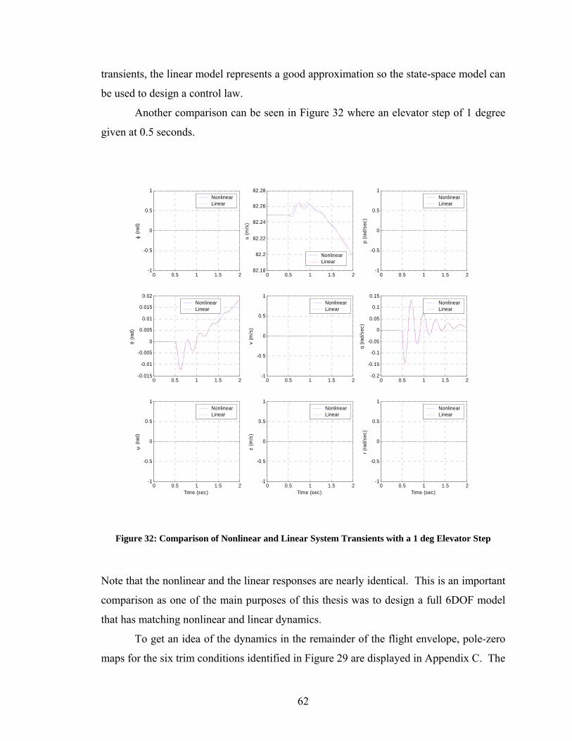
transients, the linear model represents a good approximation so the state-space model can

be used to design a control law.

Another comparison can be seen in Figure 32 where an elevator step of 1 degree

given at 0.5 seconds.

0 0.5 1 1.5 2-1

-0.5

0

0.5

1

φ (ra

d)

NonlinearLinear

0 0.5 1 1.5 2-0.015

-0.01

-0.005

0

0.005

0.01

0.015

0.02

θ (ra

d)

NonlinearLinear

0 0.5 1 1.5 2-1

-0.5

0

0.5

1

ψ (r

ad)

Time (sec)

NonlinearLinear

0 0.5 1 1.5 282.18

82.2

82.22

82.24

82.26

82.28

u (m

/s)

NonlinearLinear

0 0.5 1 1.5 2-1

-0.5

0

0.5

1

v (m

/s)

NonlinearLinear

0 0.5 1 1.5 2-1

-0.5

0

0.5

1

z (m

/s)

Time (sec)

NonlinearLinear

0 0.5 1 1.5 2-1

-0.5

0

0.5

1

p (ra

d/se

c)

NonlinearLinear

0 0.5 1 1.5 2-0.2

-0.15

-0.1

-0.05

0

0.05

0.1

0.15

q (ra

d/se

c)

NonlinearLinear

0 0.5 1 1.5 2-1

-0.5

0

0.5

1

r (ra

d/se

c)

Time (sec)

NonlinearLinear

Figure 32: Comparison of Nonlinear and Linear System Transients with a 1 deg Elevator Step

Note that the nonlinear and the linear responses are nearly identical. This is an important

comparison as one of the main purposes of this thesis was to design a full 6DOF model

that has matching nonlinear and linear dynamics.

To get an idea of the dynamics in the remainder of the flight envelope, pole-zero

maps for the six trim conditions identified in Figure 29 are displayed in Appendix C. The

62

basic conclusion from those results is that as the velocity increases, the plant becomes

more unstable.

Also displayed in Appendix C is the state-space matrix for a straight-and-level

flight condition with a forward velocity of 88.25 m/s so that these results may be readily

verified by other researchers.

7 Control Law Design The objective of a control system is to make the output y behave in a desired way

by manipulating the plant input Δ. The regulator problem is to manipulate Δ to

counteract the effect of a disturbance d. The servo problem is to manipulate Δ to keep the

output close to a given reference input r. Thus, in both cases we want the control error

rye −= to be small. The algorithm for adjusting Δ based on the available information

is the controller K. To arrive at a good design for K, a priori information is needed about

the expected disturbances and reference inputs, and of the plant model (G) and the

disturbance model (Gd). In this thesis, control design makes use of the linear models for

the form

dGGy d+Δ= Equation 60

A major source of difficulty is that the models G and Gd are approximations and

may be inaccurate and can possibly change with time (when planing for instance). In

particular, inaccuracy in G may cause problems because the plant will be part of the

feedback loop. To deal with such a problem, there is the concept of model uncertainty.

For example, instead of a single nominal model G, the behavior of a class of models,

, where the “uncertainty” or “perturbation” E is bounded, but otherwise

unknown. In most cases, weighting functions w(s) are used to express E = wΛ in terms

of the normalized perturbations, Λ, where the magnitude (norm) of Λ is less than or equal

to 1.

EGGp +=

When considering such a design process, the following terms are useful:

• Nominal Stability (NS): The nominal system is stable with no uncertainty.

63

• Nominal Performance (NP): The system satisfies the performance specifications

with no model uncertainty.

• Robust Stability (RS): The system is stable for all perturbed plans about the

nominal model up to worst-case model uncertainty.

• Robust Performance (RP): The system satisfies the performance specifications

for all perturbed plants about the nominal model up to the worst-case model

uncertainty.

7.1 Transfer Functions

The remainder of this thesis makes extensive use of transfer functions, G(s), and

of the frequency domain, which are very useful in applications for the following reasons:

• Invaluable insights are obtained from simple frequency-dependent plots.

• Important concepts for feedback such as bandwidth and peaks of closed-loop

transfer functions may be defined.

• G(jω) gives the response to sinusoidal input of frequency ω.

• A series interconnection of systems corresponds in the frequency domain to

multiplication of the individual transfer functions, whereas in the time domain,

the evaluation of complicated convolution integrals is required.

• Poles and zeros appear explicitly in factorized scaler transfer functions.

• Uncertainty is more easily handled in the frequency domain. This is related to the

fact that two systems can be described as close (i.e. have similar behavior) if the

frequency responses are similar. On the other hand, a small change in a

parameters in a state-space description can result in an entirely different system

response.

Reconsider the linear, time invariant system from Equation 55 whose input-output

responses are governed by linear ODE’s with constant coefficients.

Δ+=Δ+=

DCxyBAxx

64

For a proper system, with the number of poles greater than or equal to the number of

zeros, the transfer function can be written from the above state-space realization as

Equation 61 ( ) ( ) DBAsICsG +−= −1

Note that for multivariable system such as this torpedo model, G(s) is a matrix of transfer

functions.

For closed-loop transfer functions S denotes the sensitivity of the plant output,

and denotes the complimentary sensitivity. With negative feedback,

and , where L is the transfer function around the loop as seen

from the output. In most cases, L=GK, but if measurement dynamics are also included

then L=GKG

SIT −=

( ) 1−+= LIS ( ) 1−+= LILT

( nyGy mm += ) m. The corresponding transfer functions as seen from the

input of the plant are LI=KG or (LI=KGmG), SI=(I+LI)-1 and TI=LI(I+LI)-1.

Typical representations of closed-loop systems in block diagram form are shown

in Figure 33; case (a) is a one degree-of-freedom (1DOF) feedback loop and (b) is the

general structure.

65

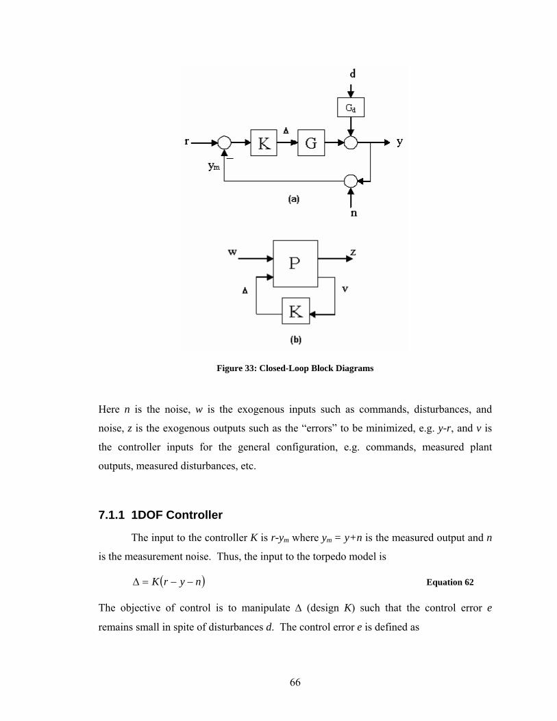
Figure 33: Closed-Loop Block Diagrams

Here n is the noise, w is the exogenous inputs such as commands, disturbances, and

noise, z is the exogenous outputs such as the “errors” to be minimized, e.g. y-r, and v is

the controller inputs for the general configuration, e.g. commands, measured plant

outputs, measured disturbances, etc.

7.1.1 1DOF Controller

The input to the controller K is r-ym where ym = y+n is the measured output and n

is the measurement noise. Thus, the input to the torpedo model is

Equation 62 ( nyrK −−=Δ )

The objective of control is to manipulate Δ (design K) such that the control error e

remains small in spite of disturbances d. The control error e is defined as

66

rye −= Equation 63

where r denotes the reference point of the output.

7.1.2 Closed-Loop Transfer Functions

The plant model is written as

dGGy d+Δ= Equation 64

and for a 1DOF controller and substitution of Equation 62 into Equation 64 yields

Equation 65

( )( )

( ) ( ) ( ) nGKGKIdGGKIrGKGKIy

GKndGGKryGKIdGnyrGKy

T

d

ST

d

d

44 344 21434 2144 344 21111 −−− +−+++=

−+=++−−=

Equation 65 represents the closed-loop response.

The control error is

TndSGSrrye d −+−=−= Equation 66

The corresponding plant input signal is

KSndKSGKSr d −−=Δ

From the above equations, it is clear that S is the closed-loop transfer function

from the output disturbances to the outputs, while T is the closed-loop transfer function

from the reference signals to the outputs. The term complimentary sensitivity follows

from the identity:

Equation 67 ITS =+

This is a fundamental design constraint for the control designer. What it means is that

there is ultimately a trade-off between disturbance rejection and closed-loop

performance; the designer cannot improve one without hindering the other.

67

7.2 Continuous-Time Linear Quadratic Controller

There are many methods used today to design controllers, some better than others

depending on the application. Common methods include PID, LQR, LQG, H∞, μ,

Dynamic Inversion, etc. However, since the focus of this thesis is really to define the

torpedo dynamic model, just a “simple” linear quadratic regulator (LQR) stabilizing

controller is synthesized here. The purpose being that this provides a stepping-stone to

further the control design process.

The LQR is a cornerstone of modern optimal control design. It has a wide range

of relevance, because many systems are linear to begin with, and in this case, the torpedo

model can be linearized when operating near an equilibrium point.

To design the optimal LQR, the design engineer must first select the design

parameter weight matrices Q (the state weighting) and R (the control weighting) in the

performance index shown in Equation 68.

Equation 68 [∫ ΔΔ+=1

0

t

t

TT dtRQxxJ ]

Q and R are symmetric matrices of design parameters chosen by the designer depending

on the control objectives. The weight matrix Q is assumed positive-semidefinite ( )0≥Q .

Thus Q has nonnegative eigenvalues so that xTQx is nonnegative for all x. Likewise, it

will be assumed that R is positive definite (R > 0), that is, R has positive eigenvalues so

that for all Δ. In this case, J is always bounded below zero, so that a sensible

minimization problem results. Since the squares of the states and control inputs occur in

Equation 68, the performance index is a form of generalized energy and minimizing it

will keep the states and controls small.

0>ΔΔ RT

For starting purposes, the gains for Q and R used in the original Anteon model

provide a good starting point. Thus, the weighting matrices chosen are

( )( ).011.01111

1.05.01.0000111diagRdiagQ

==

68

The LQR design procedure is in stark contrast to classical control design where

the gain matrix K is selected directly. In modern optimal control design, some parameter

matrices Q and R are selected by the engineer. Then, the feedback gain K is

automatically given by matrix design equations (see MATLAB’s lqr command). This

has the significant advantages of allowing all the control loops in a multiloop system to

be closed simultaneously, while guaranteeing closed-loop stability.

7.2.1 Closed-Loop Dynamics

Once the LQR controller has been defined, system dynamics can be analyzed and

simulated time histories can be examined.

As expected the LQR design created a stable closed-loop system as is shown in

Figure 34 where the closed-loop poles and zeros are presented.

Notice that there are no RHP poles in the system. This means that our system is

stable. However, note that there are two very small damping ratios of about 0.28 and

four poles that have large frequencies. The low damping ratios means it will take longer

for some signals to come to there steady-state values and the high frequencies means that

there will be some transients that have fast oscillations and also means that faster, more

expensive actuators would be needed to perform the necessary control action.

69

-30 -25 -20 -15 -10 -5 0-30

-20

-10

0

10

20

30

0.17 0.08

0.080.170.280.380.50.64

0.8

0.94

5

0.280.380.50.64

0.8

0.94

10

15

20

25

25

5

10

15

20

Closed-Loop Pole-Zero Map

Real Axis

Imag

inar

y Ax

is

Figure 34:Closed-Loop Pole-Zero Map of Nominal System with LQR Controller

Note that the large negative pole at -536 (lies on the Real axis) is not shown in the above

pole-zero map.

Figure 35 displays the nonlinear (solid, blue line) and linear (red, dashed line)

transients of a closed-loop system that utilizes the designed LQR controller after a step in

the yaw-rate state, r, with magnitude of 1 deg/sec at 0.5 sec.

70

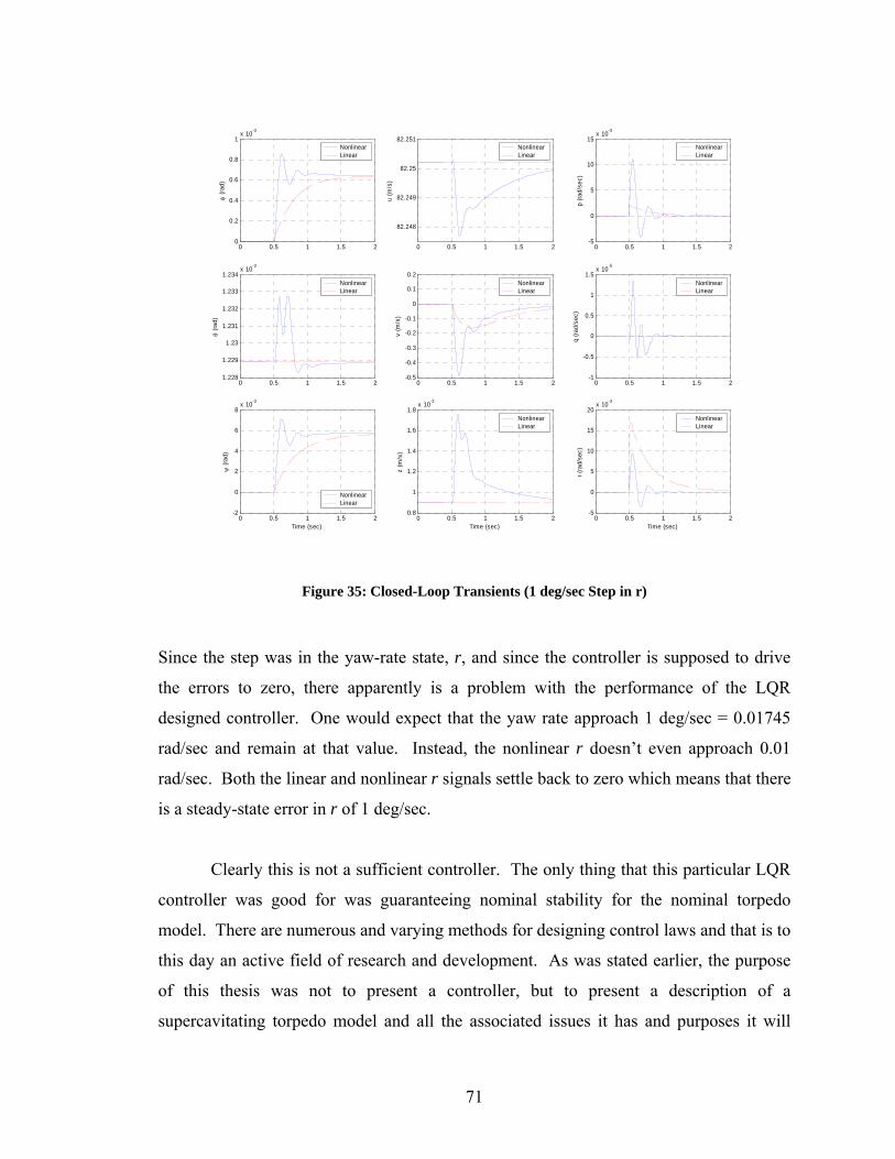
0 0.5 1 1.5 20

0.2

0.4

0.6

0.8

1x 10-3

φ (ra

d)

NonlinearLinear

0 0.5 1 1.5 21.228

1.229

1.23

1.231

1.232

1.233

1.234x 10-3

θ (ra

d)

NonlinearLinear

0 0.5 1 1.5 2-2

0

2

4

6

8x 10-3

ψ (r

ad)

Time (sec)

NonlinearLinear

0 0.5 1 1.5 2

82.248

82.249

82.25

82.251

u (m

/s)

NonlinearLinear

0 0.5 1 1.5 2-0.5

-0.4

-0.3

-0.2

-0.1

0

0.1

0.2

v (m

/s)

NonlinearLinear

0 0.5 1 1.5 20.8

1

1.2

1.4

1.6

1.8x 10-3

z (m

/s)

Time (sec)

NonlinearLinear

0 0.5 1 1.5 2-5

0

5

10

15x 10-3

p (ra

d/se

c)

NonlinearLinear

0 0.5 1 1.5 2-1

-0.5

0

0.5

1

1.5x 10-5

q (ra

d/se

c)

NonlinearLinear

0 0.5 1 1.5 2-5

0

5

10

15

20x 10-3

r (ra

d/se

c)

Time (sec)

NonlinearLinear

Figure 35: Closed-Loop Transients (1 deg/sec Step in r)

Since the step was in the yaw-rate state, r, and since the controller is supposed to drive

the errors to zero, there apparently is a problem with the performance of the LQR

designed controller. One would expect that the yaw rate approach 1 deg/sec = 0.01745

rad/sec and remain at that value. Instead, the nonlinear r doesn’t even approach 0.01

rad/sec. Both the linear and nonlinear r signals settle back to zero which means that there

is a steady-state error in r of 1 deg/sec.

Clearly this is not a sufficient controller. The only thing that this particular LQR

controller was good for was guaranteeing nominal stability for the nominal torpedo

model. There are numerous and varying methods for designing control laws and that is to

this day an active field of research and development. As was stated earlier, the purpose

of this thesis was not to present a controller, but to present a description of a

supercavitating torpedo model and all the associated issues it has and purposes it will

71

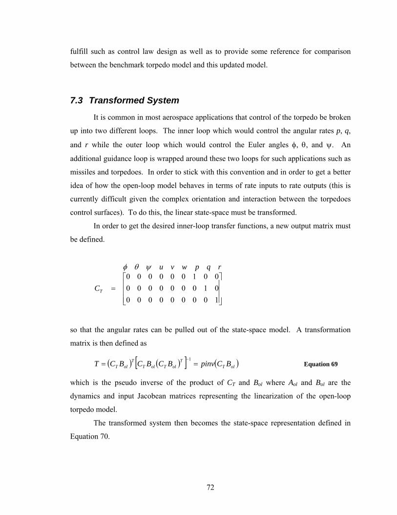
fulfill such as control law design as well as to provide some reference for comparison

between the benchmark torpedo model and this updated model.

7.3 Transformed System

It is common in most aerospace applications that control of the torpedo be broken

up into two different loops. The inner loop which would control the angular rates p, q,

and r while the outer loop which would control the Euler angles φ, θ, and ψ. An

additional guidance loop is wrapped around these two loops for such applications such as

missiles and torpedoes. In order to stick with this convention and in order to get a better

idea of how the open-loop model behaves in terms of rate inputs to rate outputs (this is

currently difficult given the complex orientation and interaction between the torpedoes

control surfaces). To do this, the linear state-space must be transformed.

In order to get the desired inner-loop transfer functions, a new output matrix must

be defined.

⎥⎥⎥

⎦

⎤

⎢⎢⎢

⎣

⎡=

100000000010000000001000000

TC

rqpwvuψθφ

so that the angular rates can be pulled out of the state-space model. A transformation

matrix is then defined as

Equation 69 ( ) ( )[ ] ( olTT

olTolTT

olT BCpinvBCBCBCT ==−1 )

which is the pseudo inverse of the product of CT and BBol where Aol and BolB are the

dynamics and input Jacobean matrices representing the linearization of the open-loop

torpedo model.

The transformed system then becomes the state-space representation defined in

Equation 70.

72

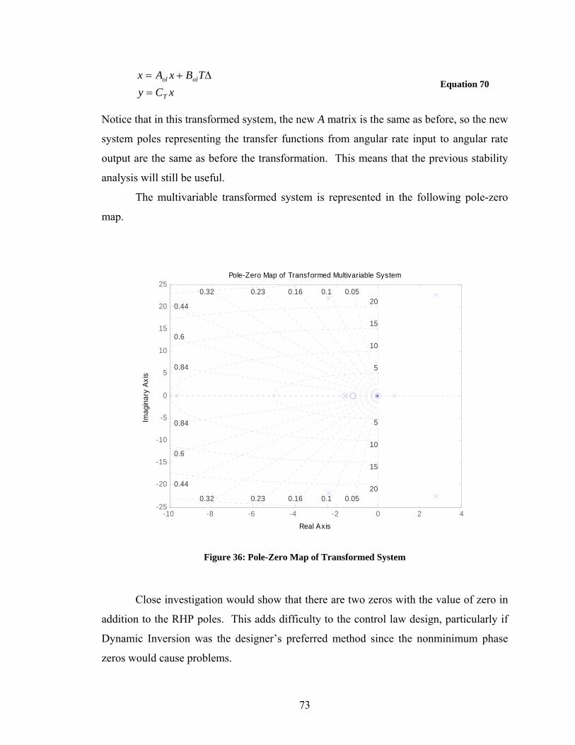
Equation 70 xCy

TBxAx

T

olol

=Δ+=

Notice that in this transformed system, the new A matrix is the same as before, so the new

system poles representing the transfer functions from angular rate input to angular rate

output are the same as before the transformation. This means that the previous stability

analysis will still be useful.

The multivariable transformed system is represented in the following pole-zero

map.

-10 -8 -6 -4 -2 0 2 4-25

-20

-15

-10

-5

0

5

10

15

20

25

0.05

0.84

0.050.10.160.230.32

0.44

0.6

0.84

0.10.160.230.32

0.44

0.6

5

10

15

20

20

5

10

15

Pole-Zero Map of Transformed Multivariable System

Real Axis

Imag

inar

y Ax

is

Figure 36: Pole-Zero Map of Transformed System

Close investigation would show that there are two zeros with the value of zero in

addition to the RHP poles. This adds difficulty to the control law design, particularly if

Dynamic Inversion was the designer’s preferred method since the nonminimum phase

zeros would cause problems.

73

The purpose of this section is not necessarily to develop a controller for the inner-

loop, but rather to present a new method/model for control law design that is typically of

interest. Once a controller is designed for this inner loop, the outer-loop design for the

Euler angles becomes a much easier problem.

8 Model Uncertainty A control system is robust if it is insensitive to differences between the actual

system and the model of the system which was used to design the controller. These

differences are referred to as model/plant mismatch or simply model uncertainty.

Uncertainty in the plant model may have several origins:

1. There are always parameters in the linear model which are only known

approximately or are simply in error.

2. The parameters in the linear model may vary due to nonlinearities or changes in

the operating conditions.

3. Measurement devices have imperfections. This may even give rise to uncertainty

on the manipulated inputs, since the actual control input is often measured and

adjusted in a cascade manner. For example, this is often the case with valves used

to measure flow. In other cases limited valve resolution may cause input

uncertainty.

4. At high frequencies even the structure and the model order is unknown and the

uncertainty will always exceed 100% at some frequency.

5. Even when a very detailed model is available we may choose to work with a

simpler (low-order) nominal model and represent neglected dynamics as

“uncertainty”.

6. Finally, the controller implemented may differ from the one obtained by solving

the synthesis problem. In this case one may include uncertainty to allow for

controller order reduction and implementation inaccuracies.

74

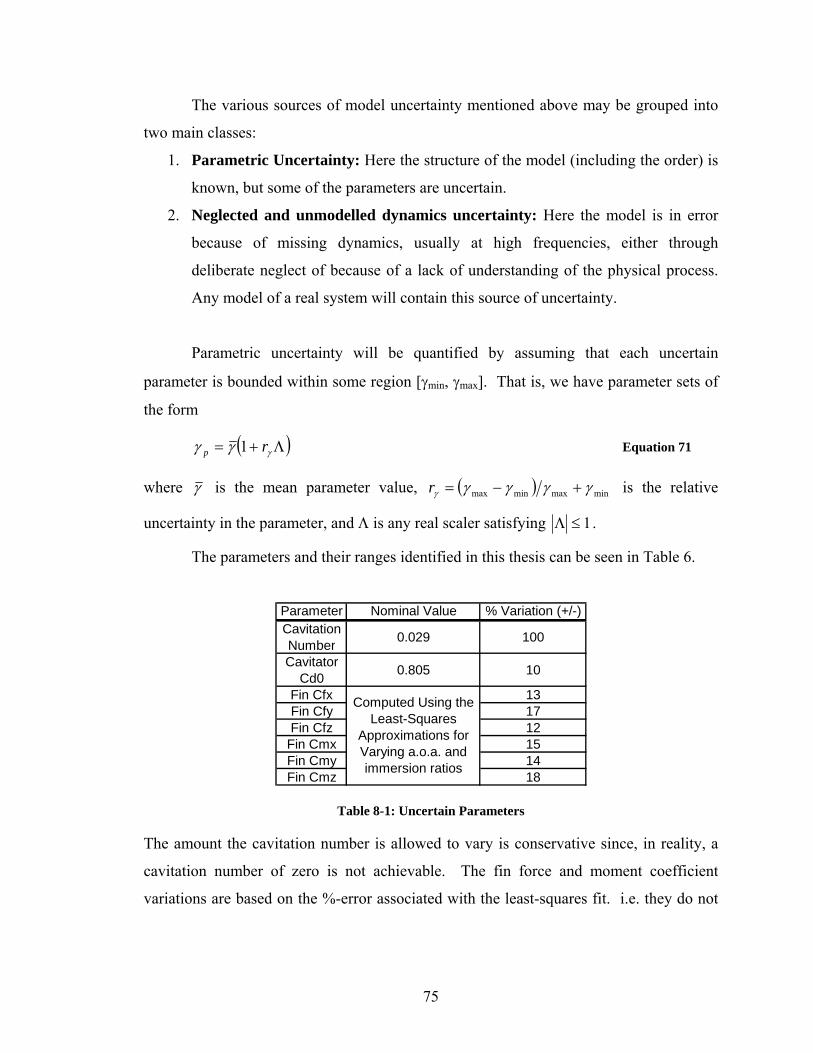
The various sources of model uncertainty mentioned above may be grouped into

two main classes:

1. Parametric Uncertainty: Here the structure of the model (including the order) is

known, but some of the parameters are uncertain.

2. Neglected and unmodelled dynamics uncertainty: Here the model is in error

because of missing dynamics, usually at high frequencies, either through

deliberate neglect of because of a lack of understanding of the physical process.

Any model of a real system will contain this source of uncertainty.

Parametric uncertainty will be quantified by assuming that each uncertain

parameter is bounded within some region [γmin, γmax]. That is, we have parameter sets of

the form

( )Λ+= γγγ rp 1 Equation 71

where γ is the mean parameter value, ( ) minmaxminmax γγγγγ +−=r is the relative

uncertainty in the parameter, and Λ is any real scaler satisfying 1≤Λ .

The parameters and their ranges identified in this thesis can be seen in Table 6.

Parameter Nominal Value % Variation (+/-)Cavitation Number 0.029 100

Cavitator Cd0 0.805 10

Fin Cfx 13Fin Cfy 17Fin Cfz 12

Fin Cmx 15Fin Cmy 14Fin Cmz 18

Computed Using the Least-Squares

Approximations for Varying a.o.a. and immersion ratios

Table 8-1: Uncertain Parameters

The amount the cavitation number is allowed to vary is conservative since, in reality, a

cavitation number of zero is not achievable. The fin force and moment coefficient

variations are based on the %-error associated with the least-squares fit. i.e. they do not

75

contain any errors due to the original model not being accurate. If one wanted to take

these type of errors into account, then the %-variation must be increased.

Neglected and unmodelled dynamics uncertainty is somewhat less precise and

thus more difficult to quantify, but it appears that the frequency domain is well suited for

this class. This leads to complex perturbations which we normalize that 1≤Λ∞

. Some

examples of unmodelled dynamics in this application would include the purposely

neglected time delays that were discussed when the cavity shape was defined.

For completeness one may consider a third class of uncertainty (which is really a

combination of the two).

3. Lumped Uncertainty: Here the uncertainty description represents one or several

sources of parametric and/or unmodelled dynamics uncertainty combined into a

single lumped perturbation of a chosen structure.

Parametric uncertainty is sometimes called structured uncertainty as it models the

uncertainty in a structured manner. Analogously, lumped dynamics uncertainty is

sometimes called unstructured uncertainty. However, one should be careful when using

these terms because there are several levels of structure, especially for MIMO systems

such as this torpedo.

8.1.1 Open-Loop Effects of Parametric Uncertainty

Some effects of model uncertainty can be seen in the way various parameters

effect the overall system dynamics. In order to examine these results, the uncertain

parameters identified above were examined by comparing the dynamics of the “nominal”

system with the systems with the minimum and maximum parameter variations. One

example of this comparison can be seen in Figure 37.

76

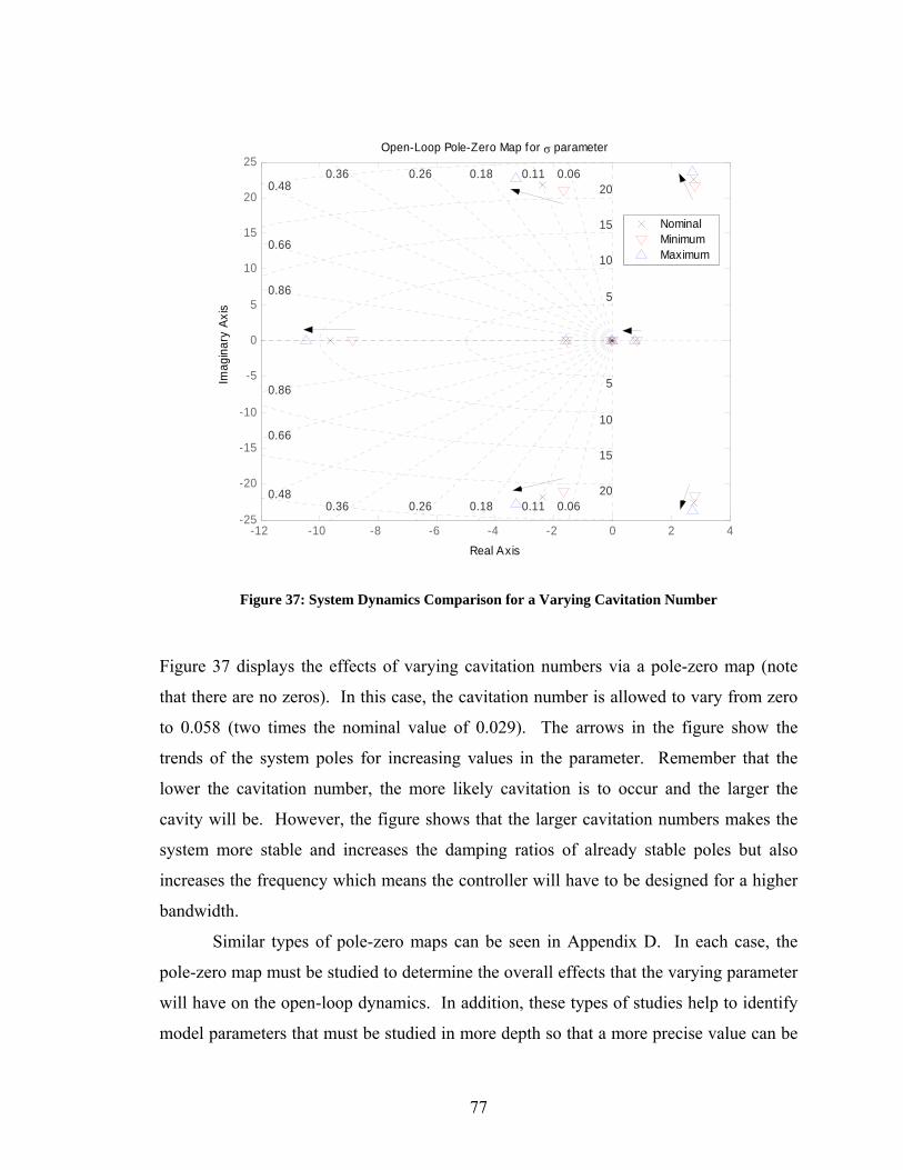
-12 -10 -8 -6 -4 -2 0 2 4-25

-20

-15

-10

-5

0

5

10

15

20

25

0.66

0.480.36 0.26 0.18 0.11 0.06

0.36 0.26 0.18 0.11 0.06

0.86 5

0.66

0.48

15

20

0.86

15

10

10

20

5

NominalMinimumMaximum

Open-Loop Pole-Zero Map for σ parameter

Real Axis

Imag

inar

y Ax

is

Figure 37: System Dynamics Comparison for a Varying Cavitation Number

Figure 37 displays the effects of varying cavitation numbers via a pole-zero map (note

that there are no zeros). In this case, the cavitation number is allowed to vary from zero

to 0.058 (two times the nominal value of 0.029). The arrows in the figure show the

trends of the system poles for increasing values in the parameter. Remember that the

lower the cavitation number, the more likely cavitation is to occur and the larger the

cavity will be. However, the figure shows that the larger cavitation numbers makes the

system more stable and increases the damping ratios of already stable poles but also

increases the frequency which means the controller will have to be designed for a higher

bandwidth.

Similar types of pole-zero maps can be seen in Appendix D. In each case, the

pole-zero map must be studied to determine the overall effects that the varying parameter

will have on the open-loop dynamics. In addition, these types of studies help to identify

model parameters that must be studied in more depth so that a more precise value can be

77

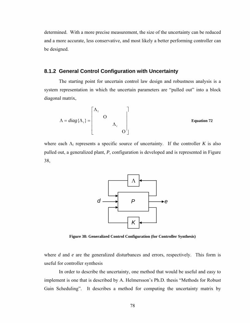
determined. With a more precise measurement, the size of the uncertainty can be reduced

and a more accurate, less conservative, and most likely a better performing controller can

be designed.

8.1.2 General Control Configuration with Uncertainty

The starting point for uncertain control law design and robustness analysis is a

system representation in which the uncertain parameters are “pulled out” into a block

diagonal matrix,

Equation 72

⎥⎥⎥⎥

⎦

⎤

⎢⎢⎢⎢

⎣

⎡

Λ

Λ

=Λ=Λ

Ο

Ο

iidiag

1

}{

where each Λi represents a specific source of uncertainty. If the controller K is also

pulled out, a generalized plant, P, configuration is developed and is represented in Figure

38,

K

Λ

P ed

Figure 38: Generalized Control Configuration (for Controller Synthesis)

where d and e are the generalized disturbances and errors, respectively. This form is

useful for controller synthesis

In order to describe the uncertainty, one method that would be useful and easy to

implement is one that is described by A. Helmersson’s Ph.D. thesis “Methods for Robust

Gain Scheduling”. It describes a method for computing the uncertainty matrix by

78

differencing the A matrices of the nominal system with the system linearized with a min

and max value of an uncertain parameter and adding the unmodelled dynamics where

appropriate. This method would save on the work needed to pull out the uncertain

parameters from the code and represent them individually, though this method would be

marginally more accurate.

Numerous references exist which describe uncertainty in more detail and how to

design a controller that takes the various types of uncertainty into consideration. If

circumstances were different, this would have been the topic of this thesis, but due to

time constraints and other commitments, this work must be handed to another.

9 General Conclusions Supercavitating torpedoes are complex systems that require an active controller,

which can ensure stability and enable the torpedo to track a target. In addition, the

control law design process requires a dynamic model that captures the physics of the

problem. Existing public 6DOF models were not able to fully capture the dynamics of

the torpedo and provide a good platform with which to design a feedback controller.

This thesis was able to design such a model and it was shown that the complex nonlinear

and simple linear model (used for control design) had matching dynamics via computer

simulation. In addition, parameters within the model that are uncertain were identified

and it was described how to incorporate them into the control law design process.

By designing such a model, several interesting properties of the torpedo were

discovered. The first, and maybe one of the most important, is that if the planing forces

are used to help support the weight of the torpedo the large planing forces occur at such a

high frequency (~50 Hz) that designing a controller with the appropriate bandwidth

would be extremely difficult in addition to expensive. This is why the thesis treated the

occurrence of planing forces as a type of operating boundary since the forces produced by

the cavitator and fins are sufficient to support the vehicles weight. This also helps to reap

the benefits of a supercavitating torpedo – less drag.

79

Unfortunately, this model is not open-loop stable as is represented by the three

open-loop system RHP poles. The states that contribute the most to these unstable poles

are roll, roll-rate, and side velocity. In addition, two of the poles have a large frequency

which means that a robustly stable controller will be much harder to design since it will

have to have a high bandwidth.

Other interesting system properties are those that are observed when model

parameters are allowed to vary. Some of the more interesting affects were noticed when

the velocity and the cavitation number was allowed to vary. For example, as the velocity

increases, the plant becomes more unstable. When considering the cavitation number,

remember that the lower the cavitation number, the more likely the cavitation occurs and

the larger the cavity will be. However, open-loop sensitivity analysis showed that the

larger cavitation number not only made the system more stable and increased the

damping ratios of already stable poles but also increased the frequency. Similar types of

effects can be seen in other parameters as well as can be seen in Appendix D.

Further work into this subject should yield a robust feedback controller and

further analysis into the worst-case performance.

80

10 Bibliography [1] Ivan N. Kirschner, et al. “Control Strategies For Supercavitating Vehicles.” University of Minnesota Graduate Seminar Series (2001) [2] Etkin, Bernard. Dynamics of Flight: Stability and Control. Second Edition Ney York, John Wiley & Sons. 1958 [3] Enns, Dale Ph. D., AEM 4303 Flight Dynamics and Control Handout. University of Minnesota, Minneapolis. Spring Semester, 2000 [4] Honeywell Technology Center, Lockheed Martin Skunk Works, Lockheed Martin Tactical Aircraft Systems, “Application of Multivariable Control Theory to Aircraft Control Laws.” WL-TR-96-3099 [5] Yuriy N. Savchenko, “SUPERCAVITATION – PROBLEMS AND PERSPECTIVES.” National Academy of Sciences − Institute of Hydromechanics, Kyiv, Ukraine, CAV2001:lecture.003. 2001 [6] Stinebring, Billet, and Lindau, Kunz, “Developed Cavitation- Cavity Dynamics.” Applied Research Laboratory, Penn State [7] Mike Elgersma, “Multibody Dynamics Using a Projection Method (Kane’s Equations).” Honeywell Labs, Internal Document, November, 1989 [8] Burah, Haim. Analytical Dynamics. Boston, WCB McGraw-Hill. 1999 [9] R.L. Waid , “Cavity Shapes for Circular Disks at Angles of Attack” California Institute of Technology Hydrodynamics Laboratory Report No. E-73.4 Pasadena, CA. 1957 [10] Blakelock, John H., Automatic Control of Aircraft and Missiles. Second Edition New York: John Wiley & Sons, Inc, 1991 [11] Kirschner, Ivan, “Numerical Modeling of Supercavitating Flows.” Anteon/Engineering Technology Center. February, 2001 [12] Savchecnko, Yu. N., “Control of Supercavitation Flow and Stability of Supercavitating Motion of Bodies.” Ukranian National Academy of Sciences – Institute of Hydromechanics. Kyiv, Ukraine. 2001 [13] Savchecnko, Yuriy N., “Supercavitation – Problems and Perspectives.” National Academy of Sciences – Institute of Hydromechanics. Kyiv, Ukraine [14] Michel, J.M., “Introduction of Cavitation and Supercavitation.” Laboratoire des

81

Ecoulements Geophysiques et Industriels. Grenoble Cedex 9, France. 2001 [15] Savchenko, Yu. N., “Experimental Investigation of Supercavitating Motion of Bodies.” Ukranian National Academy of Sciences – Institute of Hydromechanics. Kyiv, Ukraine. 2001 [16] Uhlman, J.S., Fine, N.E., and Kring, D.C., “Calculation of Added Mass and Damping Forces on Supercavitating Bodies.” Engineering Technology Center, a Division of Anteon Coorporation. Middletown, RI. 2001 [17] Streeter, Handbook of Fluid Dynamics. pp 12-25 – 12-45 [18] Savchenko, Yu. N., “Supercavitating Object Propulsion.” Ukranian National Academy of Sciences – Institute of Hydromechanics. Kyiv, Ukraine. 2001 [19] Serebryakov, Vladimmir V., “Some Models of Prediction of Supercavitation Flows Based on Slender Body Approximation.” Institute of Hydromechanics of NASU, Kieve, Ukraine. 2001 [20] Levine, William S., The Control Handbook. IEEE Press. pp 82-83, 388-393, 417-418, 457-458, 762-768, 889-891, 1105-1107 [21] Shin, Jong-Yeob, Balas, Gary J., and Packard, Andrew K., “Worst-Case Analysis of the X-38 Crew Return Vehicle Flight Control System.” Journal of Guidance, Control and Dynamics. Vol. 24, No.2, March-April 2001

82

Appendix A: Fin Force and Moment Coefficient Data Computed Directly From Anteon’s Fin Look-up Table This appendix provides graphs of the provided fin force and moment coefficient look-up table as a function of angle of attack and immersion ratios. Only limited regions of the computed/possible operating spaces are presented in order to better show the portion of the space the linearization occurs in. It should be noted, however, that these linearization values or points in the table space are based in linearization of the original Anteon model code and does not represent data for the updated/corrected model.

83

0.550.6

0.650.7

0.750.8

-2-1

01

20.5

1

1.5

2

2.5

x 10-3

Imm

Fx for Sweep = 45o

α

F x

0.550.6

0.650.7

0.750.8

-2

-1

0

1

2-0.01

-0.005

0

0.005

0.01

Imm

Mx for Sweep = 45o

α

Mx

Figure 39: Map of the x-Component of the Fin Force and Moment Coefficients

84

0.550.6

0.650.7

0.750.8

-2-1

01

2

-1.2

-1

-0.8

-0.6

-0.4

-0.2

0

x 10-3

Imm

Fy for Sweep = 45o

α

F y

0.550.6

0.650.7

0.750.8 -2

-10

12

-0.01

-0.005

0

0.005

0.01

α

My for Sweep = 45o

Imm

My

Figure 40: Map of the y-Component of the Fin Force and Moment Coefficients

85

0.550.6

0.650.7

0.750.8 -2

-1

0

1

2-0.02

-0.01

0

0.01

0.02

α

Fz for Sweep = 45o

Imm

F z

0.550.6

0.650.7

0.750.8 -2

-1

0

1

2-12

-10

-8

-6

-4

-2

x 10-4

α

Mz for Sweep = 45o

Imm

Mz

Figure 41: Map of the z-Component of the Fin Force and Moment Coefficients

86

-2 -1.5 -1 -0.5 0 0.5 1 1.5 20.6

0.8

1

1.2

1.4

1.6

1.8

2

2.2

2.4x 10-3 Fx for Sweep = 45o

α

F x

-2 -1.5 -1 -0.5 0 0.5 1 1.5 2-8

-6

-4

-2

0

2

4

6

8x 10

-3 Mx for Sweep = 45o

α

Mx

87

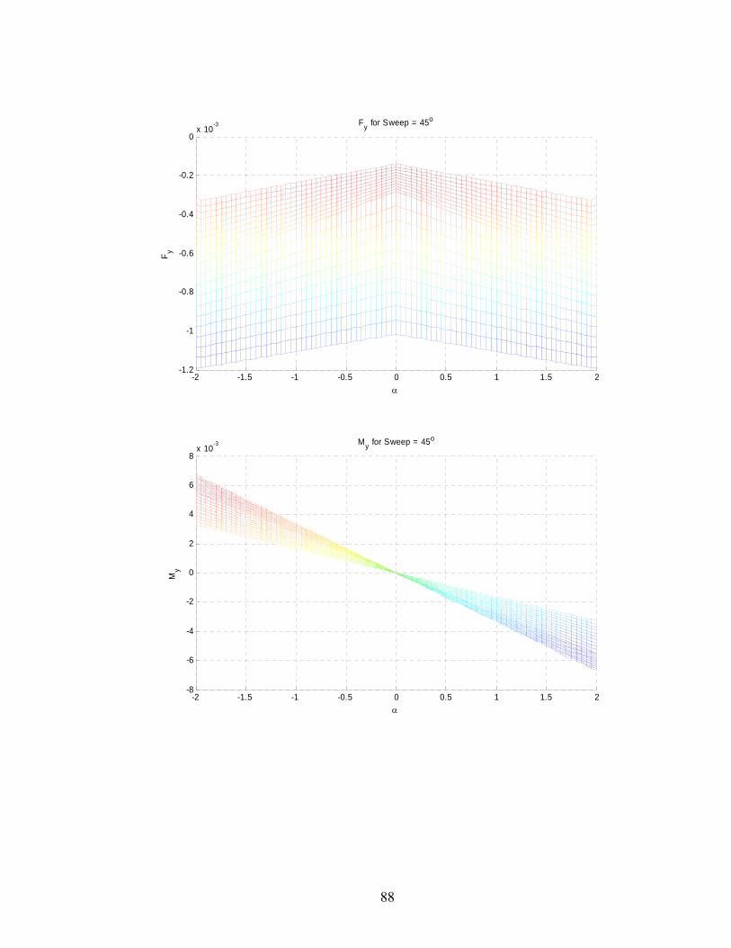
-2 -1.5 -1 -0.5 0 0.5 1 1.5 2-1.2

-1

-0.8

-0.6

-0.4

-0.2

0x 10-3 Fy for Sweep = 45o

α

F y

-2 -1.5 -1 -0.5 0 0.5 1 1.5 2-8

-6

-4

-2

0

2

4

6

8x 10

-3 My for Sweep = 45o

α

My

88

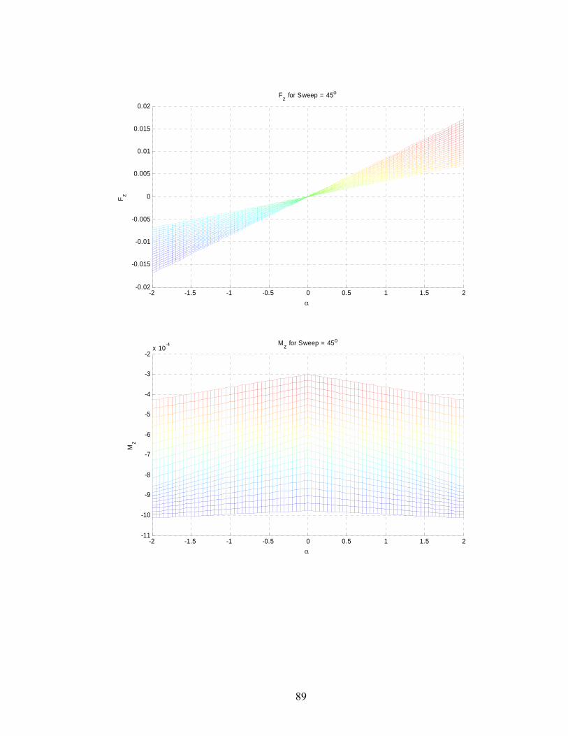
-2 -1.5 -1 -0.5 0 0.5 1 1.5 2-0.02

-0.015

-0.01

-0.005

0

0.005

0.01

0.015

0.02Fz for Sweep = 45o

α

F z

-2 -1.5 -1 -0.5 0 0.5 1 1.5 2-11

-10

-9

-8

-7

-6

-5

-4

-3

-2x 10

-4 Mz for Sweep = 45o

α

Mz

89

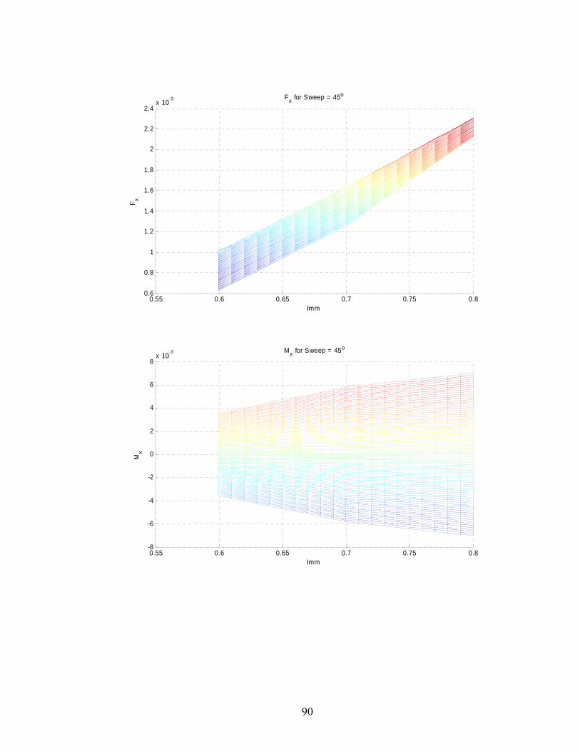
0.55 0.6 0.65 0.7 0.75 0.80.6

0.8

1

1.2

1.4

1.6

1.8

2

2.2

2.4x 10-3 Fx for Sweep = 45o

Imm

F x

0.55 0.6 0.65 0.7 0.75 0.8-8

-6

-4

-2

0

2

4

6

8x 10

-3 Mx for Sweep = 45o

Imm

Mx

90

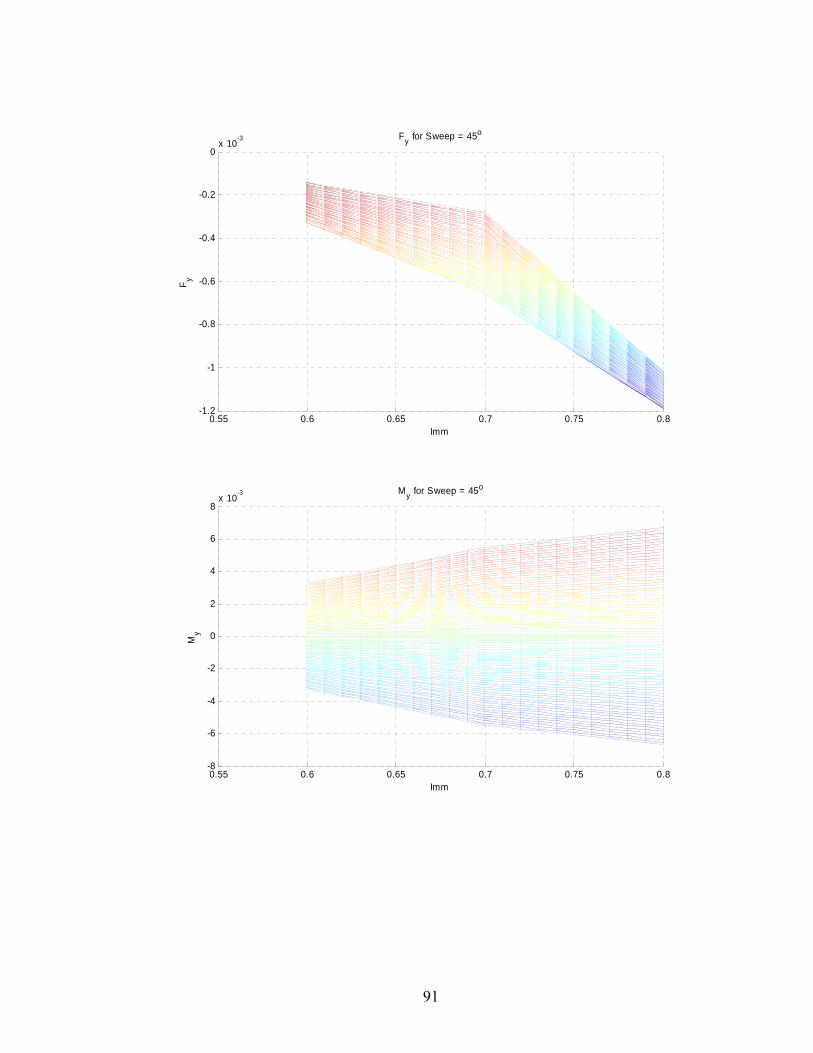
0.55 0.6 0.65 0.7 0.75 0.8-1.2

-1

-0.8

-0.6

-0.4

-0.2

0x 10-3 Fy for Sweep = 45o

Imm

F y

0.55 0.6 0.65 0.7 0.75 0.8-8

-6

-4

-2

0

2

4

6

8x 10

-3 My for Sweep = 45o

Imm

My

91

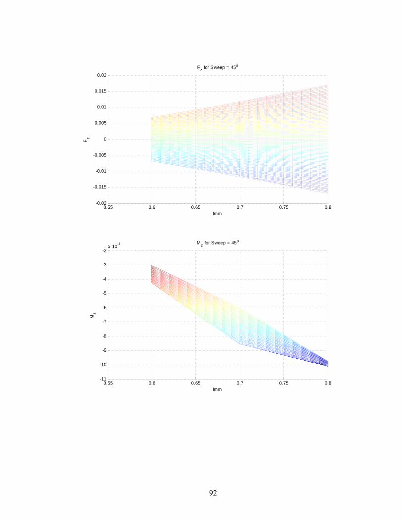
0.55 0.6 0.65 0.7 0.75 0.8-0.02

-0.015

-0.01

-0.005

0

0.005

0.01

0.015

0.02Fz for Sweep = 45o

Imm

F z

0.55 0.6 0.65 0.7 0.75 0.8-11

-10

-9

-8

-7

-6

-5

-4

-3

-2x 10

-4 Mz for Sweep = 45o

Imm

Mz

92

-2 -1.5 -1 -0.5 0 0.5 1 1.5 21

1.5

2

2.5x 10-3 Fx for Sweep = 45o

α

F x

-2 -1.5 -1 -0.5 0 0.5 1 1.5 2-8

-6

-4

-2

0

2

4

6

8x 10

-3 Mx for Sweep = 45o

α

Mx

93

-2 -1.5 -1 -0.5 0 0.5 1 1.5 2-12

-10

-8

-6

-4

-2x 10-4 Fy for Sweep = 45o

α

F y

-2 -1.5 -1 -0.5 0 0.5 1 1.5 2-8

-6

-4

-2

0

2

4

6

8x 10

-3 My for Sweep = 45o

α

My

94

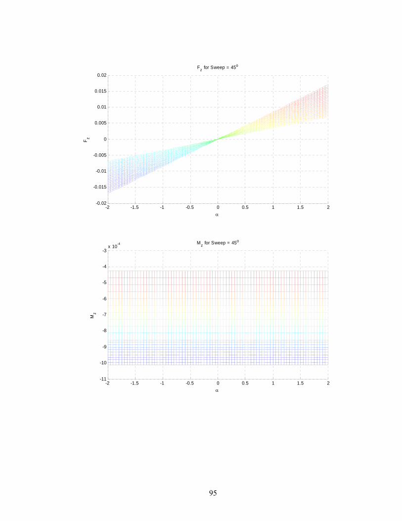
-2 -1.5 -1 -0.5 0 0.5 1 1.5 2-0.02

-0.015

-0.01

-0.005

0

0.005

0.01

0.015

0.02Fz for Sweep = 45o

α

F z

-2 -1.5 -1 -0.5 0 0.5 1 1.5 2-11

-10

-9

-8

-7

-6

-5

-4

-3x 10

-4 Mz for Sweep = 45o

α

Mz

95

-2 -1.5 -1 -0.5 0 0.5 1 1.5 2-0.02

-0.015

-0.01

-0.005

0

0.005

0.01

0.015

0.02Fz for Sweep = 45o

α

F z

-2 -1.5 -1 -0.5 0 0.5 1 1.5 2-11

-10

-9

-8

-7

-6

-5

-4

-3x 10

-4 Mz for Sweep = 45o

α

Mz

96

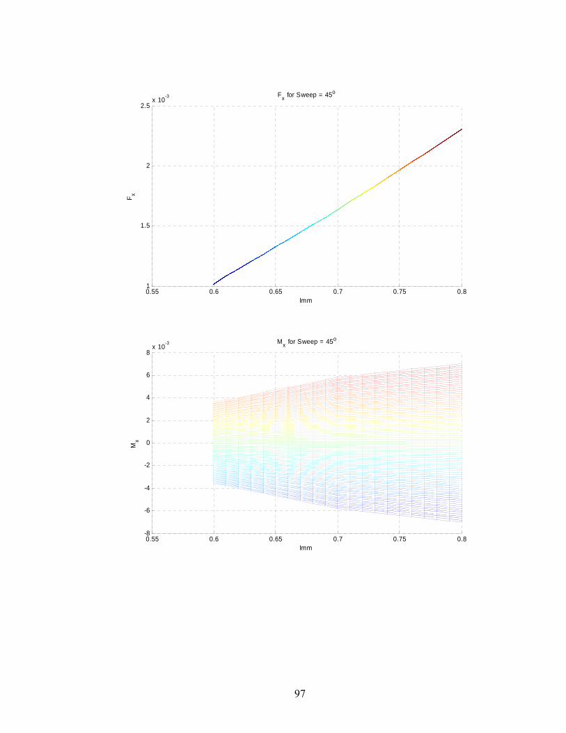
0.55 0.6 0.65 0.7 0.75 0.81

1.5

2

2.5x 10-3 Fx for Sweep = 45o

Imm

F x

0.55 0.6 0.65 0.7 0.75 0.8-8

-6

-4

-2

0

2

4

6

8x 10

-3 Mx for Sweep = 45o

Imm

Mx

97

0.55 0.6 0.65 0.7 0.75 0.8-12

-10

-8

-6

-4

-2x 10-4 Fy for Sweep = 45o

Imm

F y

0.55 0.6 0.65 0.7 0.75 0.8-8

-6

-4

-2

0

2

4

6

8x 10

-3 My for Sweep = 45o

Imm

My

98

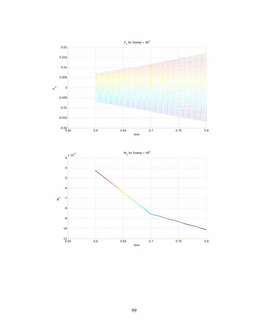
0.55 0.6 0.65 0.7 0.75 0.8-0.02

-0.015

-0.01

-0.005

0

0.005

0.01

0.015

0.02Fz for Sweep = 45o

Imm

F z

0.55 0.6 0.65 0.7 0.75 0.8-11

-10

-9

-8

-7

-6

-5

-4

-3x 10

-4 Mz for Sweep = 45o

Imm

Mz

99

Appendix B This appendix contains the Simulink and MATLAB code used to simulate the model and compute all appropriate forces.

100

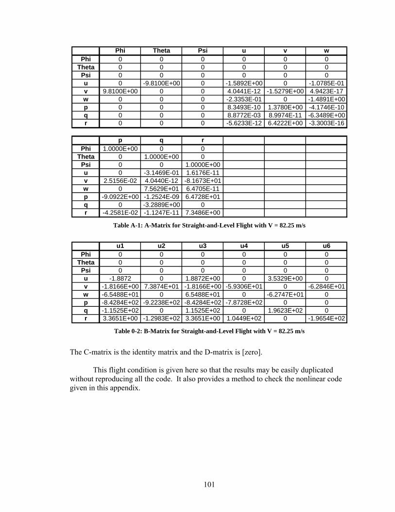
Phi Theta Psi u v wPhi 0 0 0 0 0 0

Theta 0 0 0 0 0 0Psi 0 0 0 0 0 0u 0 -9.8100E+00 0 -1.5892E+00 0 -1.0785E-01v 9.8100E+00 0 0 4.0441E-12 -1.5279E+00 4.9423E-17w 0 0 0 -2.3353E-01 0 -1.4891E+00p 0 0 0 8.3493E-10 1.3780E+00 -4.1746E-10q 0 0 0 8.8772E-03 8.9974E-11 -6.3489E+00r 0 0 0 -5.6233E-12 6.4222E+00 -3.3003E-16

p q rPhi 1.0000E+00 0 0

Theta 0 1.0000E+00 0Psi 0 0 1.0000E+00u 0 -3.1469E-01 1.6176E-11v 2.5156E-02 4.0440E-12 -8.1673E+01w 0 7.5629E+01 6.4705E-11p -9.0922E+00 -1.2524E-09 6.4728E+01q 0 -3.2889E+00 0r -4.2581E-02 -1.1247E-11 7.3486E+00

Table A-1: A-Matrix for Straight-and-Level Flight with V = 82.25 m/s

u1 u2 u3 u4 u5 u6

Phi 0 0 0 0 0 0Theta 0 0 0 0 0 0

Psi 0 0 0 0 0 0u -1.8872 0 1.8872E+00 0 3.5329E+00 0v -1.8166E+00 7.3874E+01 -1.8166E+00 -5.9306E+01 0 -6.2846E+01w -6.5488E+01 0 6.5488E+01 0 -6.2747E+01 0p -8.4284E+02 -9.2238E+02 -8.4284E+02 -7.8728E+02 0 0q -1.1525E+02 0 1.1525E+02 0 1.9623E+02 0r 3.3651E+00 -1.2983E+02 3.3651E+00 1.0449E+02 0 -1.9654E+02

Table 0-2: B-Matrix for Straight-and-Level Flight with V = 82.25 m/s

The C-matrix is the identity matrix and the D-matrix is [zero]. This flight condition is given here so that the results may be easily duplicated without reproducing all the code. It also provides a method to check the nonlinear code given in this appendix.

101

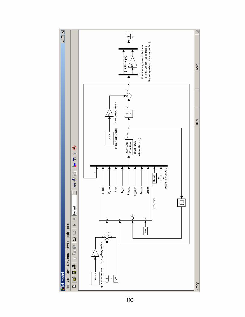
102 102

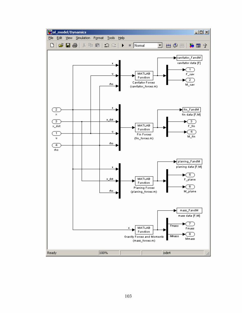
103

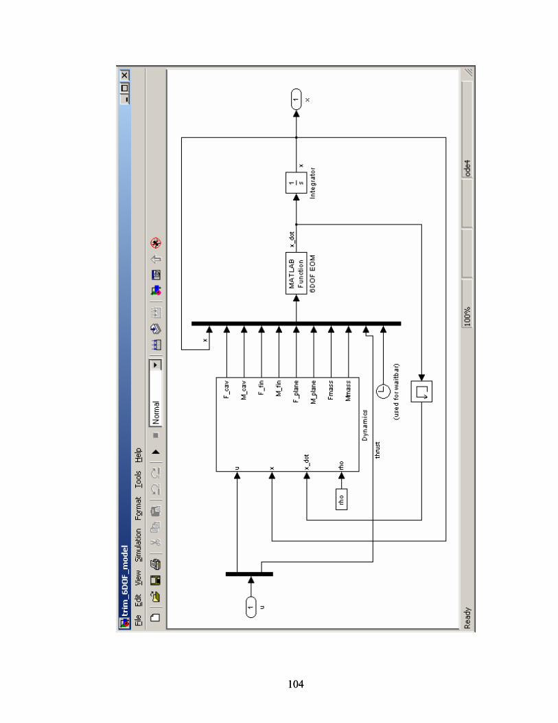
104 104

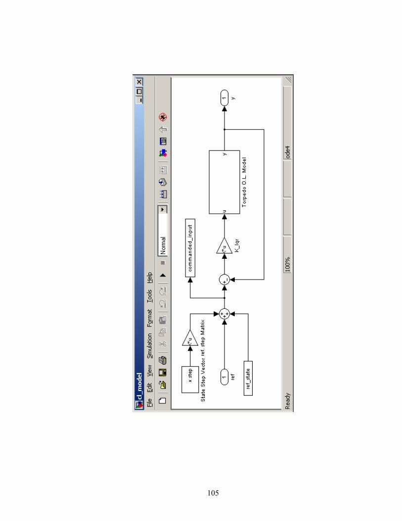
105

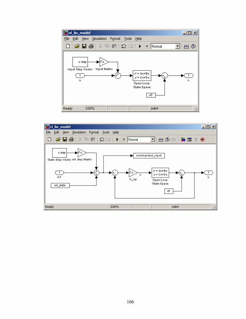
106

do_6DOF.m % This is a script designed to simulate the nonlinear 6DOF EOM and % compute the appropriate linear model. This model is slightly different % than the original EOM in that I moved the origin to the center of mass. warning off %%%%%%%%%%%%%%%%%%%%%%%%%%%%%%%%%%%%%%%%%%%%%%% % Set up model information %%%%%%%%%%%%%%%%%%%%%%%%%%%%%%%%%%%%%%%%%%%%%%% % set the global variables global planeModel mass inertia body cav cavity DELTA global sim hwait d2r = pi/180; r2d = 180/pi; % set constants and model data [mass, inertia, body, cav, cavity, rho] = setup_sim_data; %%%%%%%%%%%%%%%%%%%%%%%%%%%%%%%%%%%%%%%%%%%%%%% % Setup simulation parameters %%%%%%%%%%%%%%%%%%%%%%%%%%%%%%%%%%%%%%%%%%%%%%% sim.dt = 0.001; %sec sim.t_stop = 2; %sec sim.simulating = false; ol_sim = true; ol_lin_sim = false; cl_sim = false; cl_lin_sim = false; % set the nominal speed V = 82.25; % set the turning acceleration turnG = 0; % set the flight condition: % 'straight-and-level' % 'turn' flight_con = 'straight-and-level'; %flight_con = 'turn'; % set the initial heading initial_heading = 0; % set the output reference frame and appropriate transformation matrix mass.origin_method = 'U of MN'; %('U of MN','Anteon') switch mass.origin_method case 'U of MN' dist = [0;0;0]; case 'Anteon' dist = [mass.x_cg;0;0]';

107

otherwise error('Incorrect origin setting') end r_tilde = [0,-dist(3),dist(2); dist(3),0,-dist(1); -dist(2),dist(1),0]; R = [eye(3),r_tilde; zeros(3),eye(3)]; %%%%%%%%%%%%%%%%%%%%%%%%%%%%%%%%%%%%%%%%%%%%%%% % Define Initial/Trim Conditions %%%%%%%%%%%%%%%%%%%%%%%%%%%%%%%%%%%%%%%%%%%%%%% % set the planing model (no planing is desired) planeModel = 'Hassan'; % set the appropraite trim conditions switch flight_con case 'straight-and-level' x0 = [0,0,initial_heading,V,0,0,0,0,0]'; thrust = -1*compute_drag(x0,zeros(6,1),rho); u0 = [0,0,0,0,0,0,thrust,0,0]'; [x0,u0,y0,dx,options] = trim('trim_6DOF_model',x0,u0,[],... [1,2,3,4,5,6,7,8,9],[2,4,6,8,9]); case 'turn' x0 = [0,0,initial_heading,V,0,0,0,0,(turnG*9.81)/V]'; x_dot = zeros(9,1); s1= sin(x0(1)); c1= cos(x0(1)); s2= sin(x0(2)); c2= cos(x0(2)); tan2= tan(x0(2)); sec2= sec(x0(2)); Tb2i_ang= [1, s1*tan2, c1*tan2 ; ... 0, c1, -s1 ; ... 0, s1*sec2, c1*sec2 ]; x_dot(1:3) = Tb2i_ang*x0(7:9); x_dot(1) = 0; thrust = -1*compute_drag(x0,zeros(6,1),rho); u0 = [0,0,0,0,0,0,thrust,0,0]'; [x0,u0,y0,dx,options] = trim('trim_6DOF_model',x0,u0,[],... [9],[8,9],[],x_dot,[1,2,3,4,5,6,7,8,9]); otherwise disp('Incorrect flight condition setting') return end % check for engineering zeros in x0 and u0 tol = 1e-9; for i = 1:length(x0) if abs(x0(i)) < tol x0(i) = 0; end end for i = 1:length(u0) if abs(u0(i)) < tol u0(i) = 0; end end % display the trim conditions disp(' ')

108

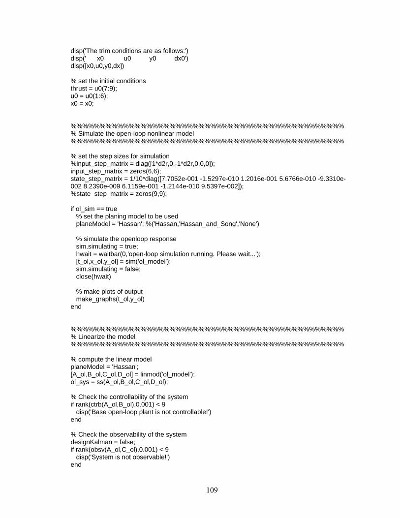
disp('The trim conditions are as follows:') disp(' x0 u0 y0 dx0') disp([x0,u0,y0,dx]) % set the initial conditions thrust = u0(7:9); u0 = u0(1:6); x0 = x0; %%%%%%%%%%%%%%%%%%%%%%%%%%%%%%%%%%%%%%%%%%%%%%% % Simulate the open-loop nonlinear model %%%%%%%%%%%%%%%%%%%%%%%%%%%%%%%%%%%%%%%%%%%%%%% % set the step sizes for simulation %input_step_matrix = diag([1*d2r,0,-1*d2r,0,0,0]); input_step_matrix = zeros(6,6); state_step_matrix = 1/10*diag([7.7052e-001 -1.5297e-010 1.2016e-001 5.6766e-010 -9.3310e-002 8.2390e-009 6.1159e-001 -1.2144e-010 9.5397e-002]); %state_step_matrix = zeros(9,9); if ol_sim == true % set the planing model to be used planeModel = 'Hassan'; %('Hassan,'Hassan_and_Song','None') % simulate the openloop response sim.simulating = true; hwait = waitbar(0,'open-loop simulation running. Please wait...'); [t_ol,x_ol,y_ol] = sim('ol_model'); sim.simulating = false; close(hwait) % make plots of output make_graphs(t_ol,y_ol) end %%%%%%%%%%%%%%%%%%%%%%%%%%%%%%%%%%%%%%%%%%%%%%% % Linearize the model %%%%%%%%%%%%%%%%%%%%%%%%%%%%%%%%%%%%%%%%%%%%%%% % compute the linear model planeModel = 'Hassan'; [A_ol,B_ol,C_ol,D_ol] = linmod('ol_model'); ol_sys = ss(A_ol,B_ol,C_ol,D_ol); % Check the controllability of the system if rank(ctrb(A_ol,B_ol),0.001) < 9 disp('Base open-loop plant is not controllable!') end % Check the observability of the system designKalman = false; if rank(obsv(A_ol,C_ol),0.001) < 9 disp('System is not observable!') end

109

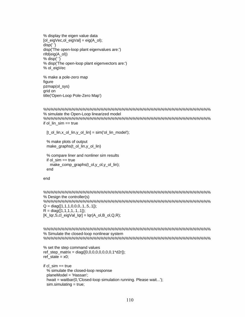
% display the eigen value data [ol_eigVec,ol_eigVal] = eig(A_ol); disp(' ') disp('The open-loop plant eigenvalues are:') rifd(eig(A_ol)) % disp(' ') % disp('The open-loop plant eigenvectors are:') % ol_eigVec % make a pole-zero map figure pzmap(ol_sys) grid on title('Open-Loop Pole-Zero Map') %%%%%%%%%%%%%%%%%%%%%%%%%%%%%%%%%%%%%%%%%%%%%%% % simulate the Open-Loop linearized model %%%%%%%%%%%%%%%%%%%%%%%%%%%%%%%%%%%%%%%%%%%%%%% if ol_lin_sim == true [t_ol_lin,x_ol_lin,y_ol_lin] = sim('ol_lin_model'); % make plots of output make_graphs(t_ol_lin,y_ol_lin) % compare liner and nonliner sim results if ol_sim == true make_comp_graphs(t_ol,y_ol,y_ol_lin); end end %%%%%%%%%%%%%%%%%%%%%%%%%%%%%%%%%%%%%%%%%%%%%%% % Design the controller(s) %%%%%%%%%%%%%%%%%%%%%%%%%%%%%%%%%%%%%%%%%%%%%%% Q = diag([1,1,1,0,0,0,.1,.5,.1]); R = diag([1,1,1,1,.1,.1]); [K_lqr,S,cl_eigVal_lqr] = lqr(A_ol,B_ol,Q,R); %%%%%%%%%%%%%%%%%%%%%%%%%%%%%%%%%%%%%%%%%%%%%%% % Simulate the closed-loop nonlinear system %%%%%%%%%%%%%%%%%%%%%%%%%%%%%%%%%%%%%%%%%%%%%%% % set the step command values ref_step_matrix = diag([0,0,0,0,0,0,0,0,1*d2r]); ref_state = x0; if cl_sim == true % simulate the closed-loop response planeModel = 'Hassan'; hwait = waitbar(0,'Closed-loop simulation running. Please wait...'); sim.simulating = true;

110

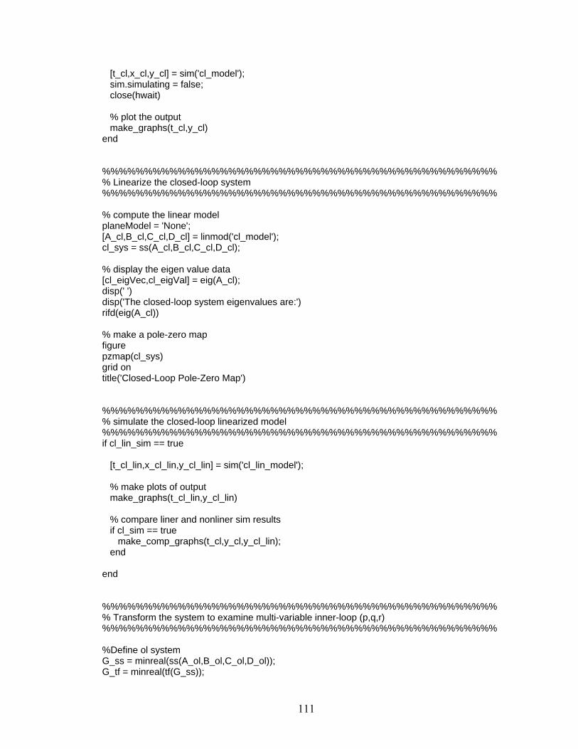
[t_cl,x_cl,y_cl] = sim('cl_model'); sim.simulating = false; close(hwait) % plot the output make_graphs(t_cl,y_cl) end %%%%%%%%%%%%%%%%%%%%%%%%%%%%%%%%%%%%%%%%%%%%%%% % Linearize the closed-loop system %%%%%%%%%%%%%%%%%%%%%%%%%%%%%%%%%%%%%%%%%%%%%%% % compute the linear model planeModel = 'None'; [A_cl,B_cl,C_cl,D_cl] = linmod('cl_model'); cl_sys = ss(A_cl,B_cl,C_cl,D_cl); % display the eigen value data [cl_eigVec,cl_eigVal] = eig(A_cl); disp(' ') disp('The closed-loop system eigenvalues are:') rifd(eig(A_cl)) % make a pole-zero map figure pzmap(cl_sys) grid on title('Closed-Loop Pole-Zero Map') %%%%%%%%%%%%%%%%%%%%%%%%%%%%%%%%%%%%%%%%%%%%%%% % simulate the closed-loop linearized model %%%%%%%%%%%%%%%%%%%%%%%%%%%%%%%%%%%%%%%%%%%%%%% if cl_lin_sim == true [t_cl_lin,x_cl_lin,y_cl_lin] = sim('cl_lin_model'); % make plots of output make_graphs(t_cl_lin,y_cl_lin) % compare liner and nonliner sim results if cl_sim == true make_comp_graphs(t_cl,y_cl,y_cl_lin); end end %%%%%%%%%%%%%%%%%%%%%%%%%%%%%%%%%%%%%%%%%%%%%%% % Transform the system to examine multi-variable inner-loop (p,q,r) %%%%%%%%%%%%%%%%%%%%%%%%%%%%%%%%%%%%%%%%%%%%%%% %Define ol system G_ss = minreal(ss(A_ol,B_ol,C_ol,D_ol)); G_tf = minreal(tf(G_ss));

111

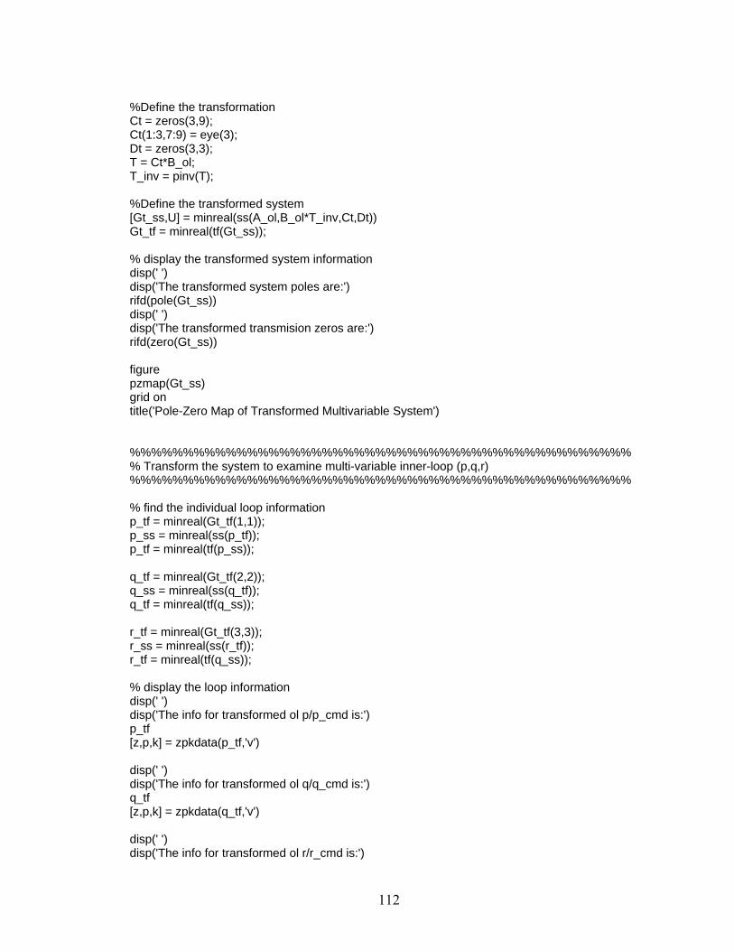
%Define the transformation Ct = zeros(3,9); Ct(1:3,7:9) = eye(3); Dt = zeros(3,3); T = Ct*B_ol; T_inv = pinv(T); %Define the transformed system [Gt_ss,U] = minreal(ss(A_ol,B_ol*T_inv,Ct,Dt)) Gt_tf = minreal(tf(Gt_ss)); % display the transformed system information disp(' ') disp('The transformed system poles are:') rifd(pole(Gt_ss)) disp(' ') disp('The transformed transmision zeros are:') rifd(zero(Gt_ss)) figure pzmap(Gt_ss) grid on title('Pole-Zero Map of Transformed Multivariable System') %%%%%%%%%%%%%%%%%%%%%%%%%%%%%%%%%%%%%%%%%%%%%%% % Transform the system to examine multi-variable inner-loop (p,q,r) %%%%%%%%%%%%%%%%%%%%%%%%%%%%%%%%%%%%%%%%%%%%%%% % find the individual loop information p_tf = minreal(Gt_tf(1,1)); p_ss = minreal(ss(p_tf)); p_tf = minreal(tf(p_ss)); q_tf = minreal(Gt_tf(2,2)); q_ss = minreal(ss(q_tf)); q_tf = minreal(tf(q_ss)); r_tf = minreal(Gt_tf(3,3)); r_ss = minreal(ss(r_tf)); r_tf = minreal(tf(q_ss)); % display the loop information disp(' ') disp('The info for transformed ol p/p_cmd is:') p_tf [z,p,k] = zpkdata(p_tf,'v') disp(' ') disp('The info for transformed ol q/q_cmd is:') q_tf [z,p,k] = zpkdata(q_tf,'v') disp(' ') disp('The info for transformed ol r/r_cmd is:')

112

r_tf [z,p,k] = zpkdata(r_tf,'v')

113

setup_sim_data.m function [mass, inertia, body, cav, cavity, rho] = setup_sim_data() global DELTA %%%%%%%%%%%%%%%%%%%%%%%%%%%%%%%%%%%%%%%%%%%%%%% % Define the uncertain parameters and the their associated range of values % (in percent difference) %%%%%%%%%%%%%%%%%%%%%%%%%%%%%%%%%%%%%%%%%%%%%%% % uncertainty in cavitator Cd0 DELTA.Cd0_range = [-.05 0 0.05]; % +/- 5% DELTA.Cd0_rval = 2; % uncertainty in the fin force and moment coefficients DELTA.Cfin_range = [-.13, 0, .13; -.17, 0, .17; -.12, 0, .12; -.15, 0, .15; -.14, 0, .14; -.18, 0, .18]; DELTA.Cfin_rval = 2; DELTA.Cfin_coef = 1; % uncertainty in the cavitation number DELTA.sigma_range = [-.029 0 .029]; DELTA.sigma_rval = 2; % uncertainty in the position of the center of gravity. This could account % for variations in mass as fuel is depleted much like an aircraft deals % with forward-heavy and aft-light conditions. DELTA.xcg_range = [-.1 0 .1]; %+/- 10% DELTA.xcg_rval = 2; %%%%%%%%%%%%%%%%%%%%%%%%%%%%%%%%%%%%%%%%%%%%%%% % define the water density % NOTE: This constant should actually become a function since the density % changes with water depth %%%%%%%%%%%%%%%%%%%%%%%%%%%%%%%%%%%%%%%%%%%%%%% rho = 1024; %%%%%%%%%%%%%%%%%%%%%%%%%%%%%%%%%%%%%%%%%%%%%%% % torpedo body related constants (geometry) %%%%%%%%%%%%%%%%%%%%%%%%%%%%%%%%%%%%%%%%%%%%%%% % maximum dimensions body.L = 4.064; % overall body length [m] body.R = 0.1015; % maximum body radius [m] % body/section lengths (aft of cavitator) secL = [0.0625, 0.2500, 0.59375, 0.09375]; xlast = 0; for i = 1:4 body.x1(i) = xlast; body.x2(i) = xlast + secL(i)*body.L;

114

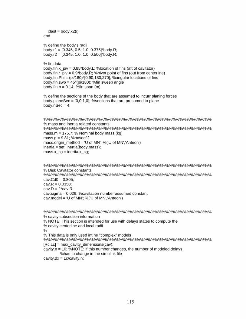
xlast = body.x2(i); end % define the body's radii body.r1 = [0.345, 0.5, 1.0, 0.375]*body.R; body.r2 = [0.345, 1.0, 1.0, 0.500]*body.R; % fin data body.fin.x_piv = 0.85*body.L; %location of fins (aft of cavitator) body.fin.r_piv = 0.9*body.R; %pivot point of fins (out from centerline) body.fin.Phi = (pi/180)*[0,90,180,270]; %angular locations of fins body.fin.swp = 45*(pi/180); %fin sweep angle body.fin.b = 0.14; %fin span (m) % define the sections of the body that are assumed to incurr planing forces body.planeSec = [0,0,1,0]; %sections that are presumed to plane body.nSec = 4; %%%%%%%%%%%%%%%%%%%%%%%%%%%%%%%%%%%%%%%%%%%%%%% % mass and inertia related constants %%%%%%%%%%%%%%%%%%%%%%%%%%%%%%%%%%%%%%%%%%%%%%% mass.m = 175.7; % Nominal body mass (kg) mass.g = 9.81; %m/sec^2 mass.origin_method = 'U of MN'; %('U of MN','Anteon') inertia = set_inertia(body,mass); mass.x_cg = inertia.x_cg; %%%%%%%%%%%%%%%%%%%%%%%%%%%%%%%%%%%%%%%%%%%%%%% % Disk Cavitator constants %%%%%%%%%%%%%%%%%%%%%%%%%%%%%%%%%%%%%%%%%%%%%%% cav.Cd0 = 0.805; cav.R = 0.0350; cav.D = 2*cav.R; cav.sigma = 0.029; %cavitation number assumed constant cav.model = 'U of MN'; %('U of MN','Anteon') %%%%%%%%%%%%%%%%%%%%%%%%%%%%%%%%%%%%%%%%%%%%%%% % cavity subsection information % NOTE: This section is intended for use with delays states to compute the % cavity centerline and local radii % % This data is only used int he "complex" models %%%%%%%%%%%%%%%%%%%%%%%%%%%%%%%%%%%%%%%%%%%%%%% [Rc,Lc] = max_cavity_dimensions(cav); cavity.n = 10; %NOTE: if this number changes, the number of modeled delays %has to change in the simulink file cavity.dx = Lc/cavity.n;

115

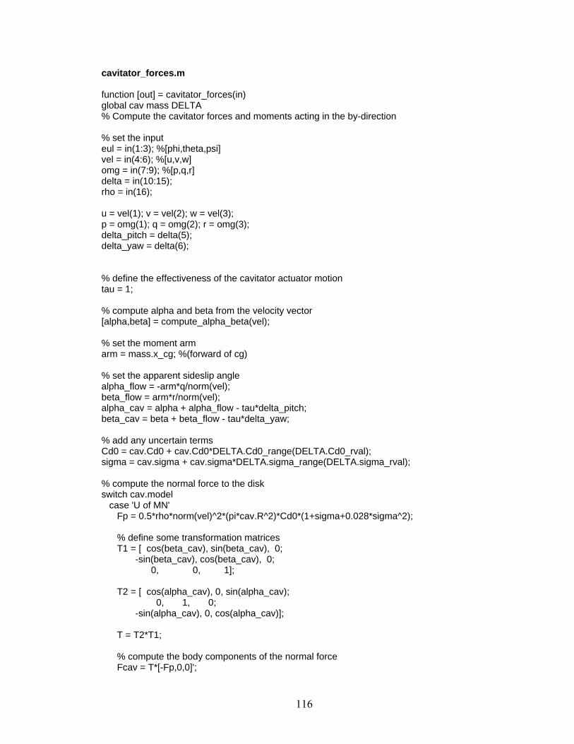
cavitator_forces.m function [out] = cavitator_forces(in) global cav mass DELTA % Compute the cavitator forces and moments acting in the by-direction % set the input eul = in(1:3); %[phi,theta,psi] vel = in(4:6); %[u,v,w] omg = in(7:9); %[p,q,r] delta = in(10:15); rho = in(16); u = vel(1); v = vel(2); w = vel(3); p = omg(1); q = omg(2); r = omg(3); delta_pitch = delta(5); delta_yaw = delta(6); % define the effectiveness of the cavitator actuator motion tau = 1; % compute alpha and beta from the velocity vector [alpha,beta] = compute_alpha_beta(vel); % set the moment arm arm = mass.x_cg; %(forward of cg) % set the apparent sideslip angle alpha_flow = -arm*q/norm(vel); beta_flow = arm*r/norm(vel); alpha_cav = alpha + alpha_flow - tau*delta_pitch; beta_cav = beta + beta_flow - tau*delta_yaw; % add any uncertain terms Cd0 = cav.Cd0 + cav.Cd0*DELTA.Cd0_range(DELTA.Cd0_rval); sigma = cav.sigma + cav.sigma*DELTA.sigma_range(DELTA.sigma_rval); % compute the normal force to the disk switch cav.model case 'U of MN' Fp = 0.5*rho*norm(vel)^2*(pi*cav.R^2)*Cd0*(1+sigma+0.028*sigma^2); % define some transformation matrices T1 = [ cos(beta_cav), sin(beta_cav), 0; -sin(beta_cav), cos(beta_cav), 0; 0, 0, 1]; T2 = [ cos(alpha_cav), 0, sin(alpha_cav); 0, 1, 0; -sin(alpha_cav), 0, cos(alpha_cav)]; T = T2*T1; % compute the body components of the normal force Fcav = T*[-Fp,0,0]';

116

case 'Anteon' % Force perpendicular to disk, drag reduced for apparent angles of attack Fp= 0.5*rho*norm(vel)^2*(pi*cav.R^2) * ... Cd0*(1+sigma+.028*sigma^2)*cos(alpha_cav)*cos(beta_cav); % Forces in body-frame of reference fx= -Fp*cos(delta_pitch)*cos(delta_yaw); fy= -Fp*cos(delta_pitch)*sin(delta_yaw); fz= Fp*sin(delta_pitch); Fcav = [fx,fy,fz]'; otherwise disp('Unknown cavitator model') end % compute the moments caused by the cavitator Mcav = cross([arm,0,0]',Fcav); % set the output out = [Fcav; Mcav]; return

117

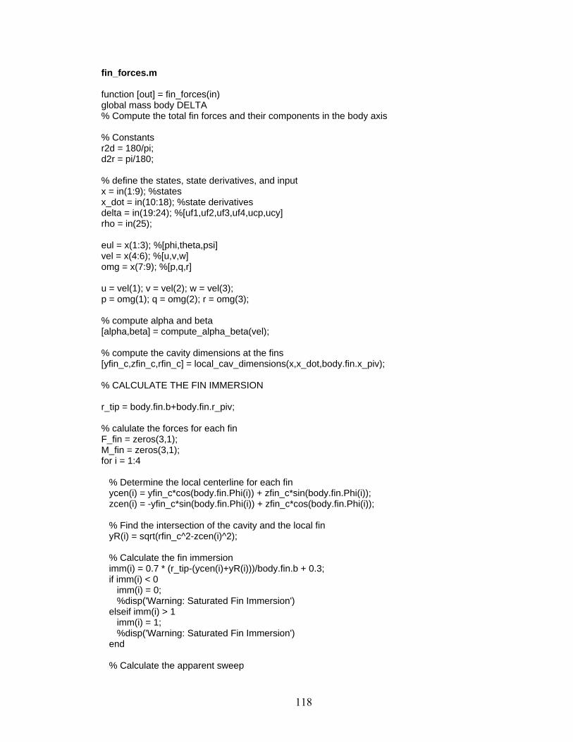
fin_forces.m function [out] = fin_forces(in) global mass body DELTA % Compute the total fin forces and their components in the body axis % Constants r2d = 180/pi; d2r = pi/180; % define the states, state derivatives, and input x = in(1:9); %states x_dot = in(10:18); %state derivatives delta = in(19:24); %[uf1,uf2,uf3,uf4,ucp,ucy] rho = in(25); eul = x(1:3); %[phi,theta,psi] vel = x(4:6); %[u,v,w] omg = x(7:9); %[p,q,r] u = vel(1); v = vel(2); w = vel(3); p = omg(1); q = omg(2); r = omg(3); % compute alpha and beta [alpha,beta] = compute_alpha_beta(vel); % compute the cavity dimensions at the fins [yfin_c,zfin_c,rfin_c] = local_cav_dimensions(x,x_dot,body.fin.x_piv); % CALCULATE THE FIN IMMERSION r_tip = body.fin.b+body.fin.r_piv; % calulate the forces for each fin F_fin = zeros(3,1); M_fin = zeros(3,1); for i = 1:4 % Determine the local centerline for each fin ycen(i) = yfin_c*cos(body.fin.Phi(i)) + zfin_c*sin(body.fin.Phi(i)); zcen(i) = -yfin_c*sin(body.fin.Phi(i)) + zfin_c*cos(body.fin.Phi(i)); % Find the intersection of the cavity and the local fin yR(i) = sqrt(rfin_c^2-zcen(i)^2); % Calculate the fin immersion imm(i) = 0.7 * (r_tip-(ycen(i)+yR(i)))/body.fin.b + 0.3; if imm(i) < 0 imm(i) = 0; %disp('Warning: Saturated Fin Immersion') elseif imm(i) > 1 imm(i) = 1; %disp('Warning: Saturated Fin Immersion') end % Calculate the apparent sweep

118

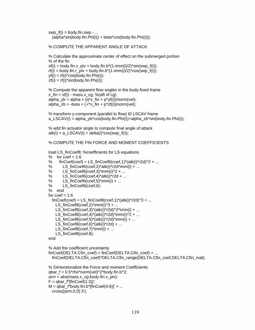
swp_f(i) = body.fin.swp - ... (alpha*sin(body.fin.Phi(i)) + beta*cos(body.fin.Phi(i))); % COMPUTE THE APPARENT ANGLE OF ATTACK % Calculate the approximate center of effect on the submerged portion % of the fin xf(i) = body.fin.x_piv + body.fin.b*(1-imm(i)/2)*sin(swp_f(i)); rf(i) = body.fin.r_piv + body.fin.b*(1-imm(i)/2)*cos(swp_f(i)); yf(i) = rf(i)*cos(body.fin.Phi(i)); zf(i) = rf(i)*sin(body.fin.Phi(i)); % Compute the apparent flow angles in the body-fixed frame x_fin = xf(i) - mass.x_cg; %(aft of cg) alpha_yb = alpha + (q*x_fin + p*yf(i))/norm(vel); alpha_zb = -beta + (-r*x_fin + p*zf(i))/norm(vel); % transform y-component (parallel to flow) t0 LSCAV frame a_LSCAV(i) = alpha_yb*cos(body.fin.Phi(i))+alpha_zb*sin(body.fin.Phi(i)); % add fin actuator angle to compute final angle of attack atk(i) = a_LSCAV(i) + delta(i)*cos(swp_f(i)); % COMPUTE THE FIN FORCE AND MOMENT COEFFICIENTS load LS_finCoef8; %coefficients for LS equations % for coef = 1:6 % finCoef(coef) = LS_finCoef6(coef,1)*(atk(i)*r2d)^2 + ... % LS_finCoef6(coef,2)*atk(i)*r2d*imm(i) + ... % LS_finCoef6(coef,3)*imm(i)^2 + ... % LS_finCoef6(coef,4)*atk(i)*r2d + ... % LS_finCoef6(coef,5)*imm(i) + ... % LS_finCoef6(coef,6); % end for coef = 1:6 finCoef(coef) = LS_finCoef8(coef,1)*(atk(i)*r2d)^3 + ... LS_finCoef8(coef,2)*imm(i)^3 + ... LS_finCoef8(coef,3)*(atk(i)*r2d)^2*imm(i) + ... LS_finCoef8(coef,4)*(atk(i)*r2d)*imm(i)^2 + ... LS_finCoef8(coef,5)*(atk(i)*r2d)*imm(i) + ... LS_finCoef8(coef,6)*(atk(i)*r2d) + ... LS_finCoef8(coef,7)*imm(i) + ... LS_finCoef8(coef,8); end % Add the coefficient uncertainty finCoef(DELTA.Cfin_coef) = finCoef(DELTA.Cfin_coef) + ... finCoef(DELTA.Cfin_coef)*DELTA.Cfin_range(DELTA.Cfin_coef,DELTA.Cfin_rval); % Dimensionalize the Force and moment Coefficients qbar_f = 0.5*rho*norm(vel)^2*body.fin.b^2; arm = abs(mass.x_cg-body.fin.x_piv); F = qbar_f*[finCoef(1:3)]'; M = qbar_f*body.fin.b*[finCoef(4:6)]' + ... cross([arm,0,0]',F);

119

% rotate the forces and moments into the corect body axis ci = cos(body.fin.Phi(i)); si = sin(body.fin.Phi(i)); F_fin(1) = F_fin(1) - F(1); F_fin(2) = F_fin(2) + F(2)*ci + F(3)*si; F_fin(3) = F_fin(3) + F(2)*si - F(3)*ci; M_fin(1) = M_fin(1) - M(1); M_fin(2) = M_fin(2) + M(2)*ci + M(3)*si; M_fin(3) = M_fin(3) + M(2)*si - M(3)*ci; end out = [F_fin;M_fin]; return

120

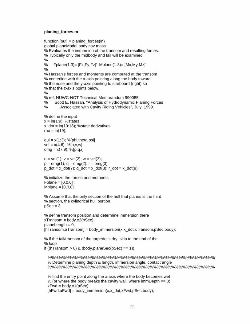
planing_forces.m function [out] = planing_forces(in) global planeModel body cav mass % Evaluates the immersion of the transom and resulting forces. % Typically only the midbody and tail will be examined. % % Fplane(1:3)= [Fx,Fy,Fz]' Mplane(1:3)= [Mx,My,Mz]' % % Hassan's forces and moments are computed at the transom % centerline with the x-axis pointing along the body toward % the nose and the y-axis pointing to starboard (right) so % that the z-axis points below. % % ref: NUWC-NOT Technical Memorandum 990085 % Scott E. Hassan, "Analysis of Hydrodynamic Planing Forces % Associated with Cavity Riding Vehicles", July, 1999. % define the input x = in(1:9); %states x_dot = in(10:18); %state derivatives rho = in(19); eul = x(1:3); %[phi,theta,psi] vel = x(4:6); %[u,v,w] omg = x(7:9); %[p,q,r] u = vel(1); v = vel(2); w = vel(3); p = omg(1); q = omg(2); r = omg(3); p_dot = x_dot(7); q_dot = x_dot(8); r_dot = x_dot(9); % initialize the forces and moments Fplane = [0,0,0]'; Mplane = [0,0,0]'; % Assume that the only section of the hull that planes is the third % section, the cylindrical hull portion pSec = 3; % define transom position and determine immersion there xTransom = body.x2(pSec); planeLength = 0; [hTransom,aTransom] = body_immersion(x,x_dot,xTransom,pSec,body); % if the tail/transom of the torpedo is dry, skip to the end of the % loop if ((hTransom > 0) & (body.planeSec(pSec) == 1)) %%%%%%%%%%%%%%%%%%%%%%%%%%%%%%%%%%%%%%%%%%%%%% % Determine planing depth & length, immersion angle, contact angle %%%%%%%%%%%%%%%%%%%%%%%%%%%%%%%%%%%%%%%%%%%%%% % find the entry point along the x-axis where the body becomes wet % (or where the body breaks the cavity wall, where immDepth == 0) xFwd = body.x1(pSec); [hFwd,aFwd] = body_immersion(x,x_dot,xFwd,pSec,body);

121

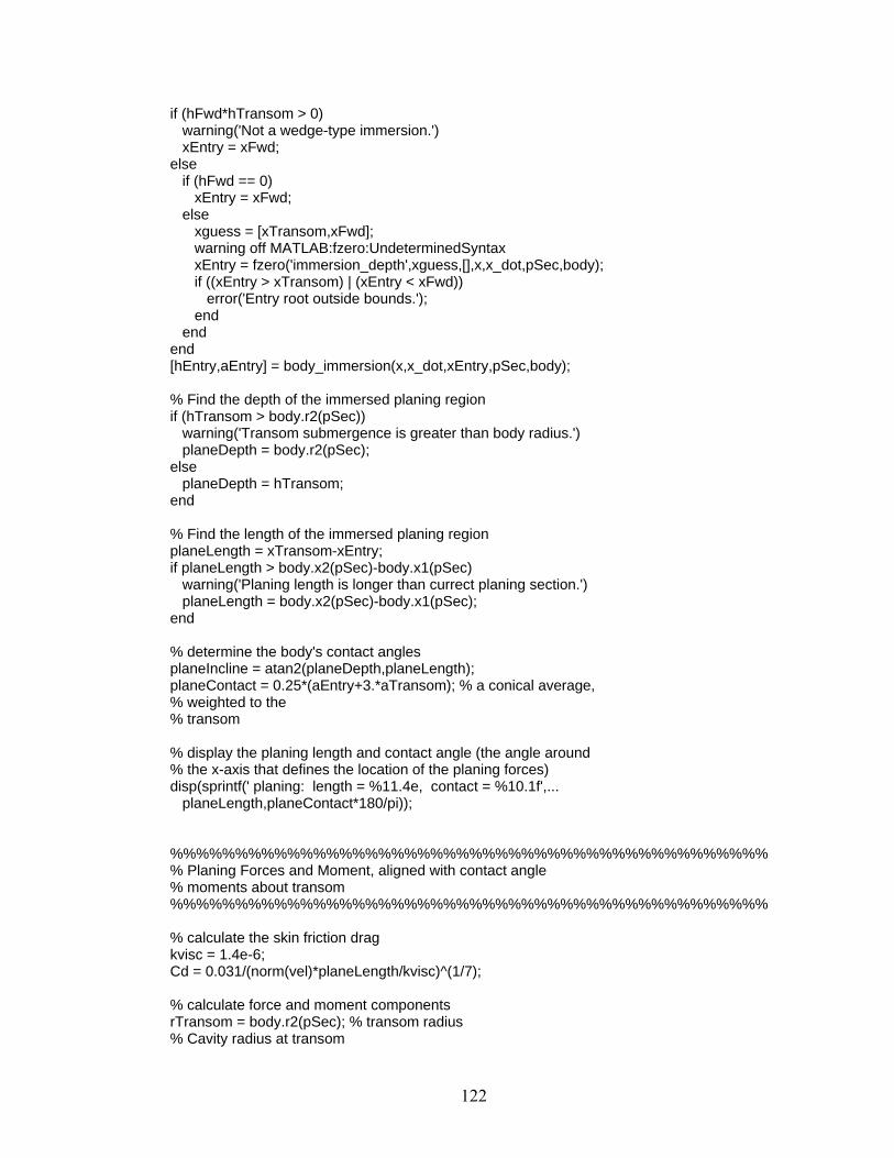
if (hFwd*hTransom > 0) warning('Not a wedge-type immersion.') xEntry = xFwd; else if (hFwd == 0) xEntry = xFwd; else xguess = [xTransom,xFwd]; warning off MATLAB:fzero:UndeterminedSyntax xEntry = fzero('immersion_depth',xguess,[],x,x_dot,pSec,body); if ((xEntry > xTransom) | (xEntry < xFwd)) error('Entry root outside bounds.'); end end end [hEntry,aEntry] = body_immersion(x,x_dot,xEntry,pSec,body); % Find the depth of the immersed planing region if (hTransom > body.r2(pSec)) warning('Transom submergence is greater than body radius.') planeDepth = body.r2(pSec); else planeDepth = hTransom; end % Find the length of the immersed planing region planeLength = xTransom-xEntry; if planeLength > body.x2(pSec)-body.x1(pSec) warning('Planing length is longer than currect planing section.') planeLength = body.x2(pSec)-body.x1(pSec); end % determine the body's contact angles planeIncline = atan2(planeDepth,planeLength); planeContact = 0.25*(aEntry+3.*aTransom); % a conical average, % weighted to the % transom % display the planing length and contact angle (the angle around % the x-axis that defines the location of the planing forces) disp(sprintf(' planing: length = %11.4e, contact = %10.1f',... planeLength,planeContact*180/pi)); %%%%%%%%%%%%%%%%%%%%%%%%%%%%%%%%%%%%%%%%%%%%%% % Planing Forces and Moment, aligned with contact angle % moments about transom %%%%%%%%%%%%%%%%%%%%%%%%%%%%%%%%%%%%%%%%%%%%%% % calculate the skin friction drag kvisc = 1.4e-6; Cd = 0.031/(norm(vel)*planeLength/kvisc)^(1/7); % calculate force and moment components rTransom = body.r2(pSec); % transom radius % Cavity radius at transom

122

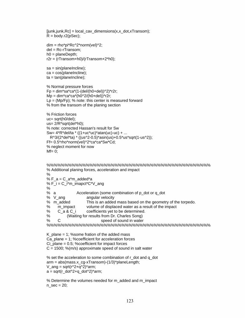
[junk,junk,Rc] = local_cav_dimensions(x,x_dot,xTransom); R = body.r2(pSec); dim = rho*pi*Rc^2*norm(vel)^2; del = Rc-rTransom; h0 = planeDepth; r2r = (rTransom+h0)/(rTransom+2*h0); sa = sin(planeIncline); ca = cos(planeIncline); ta = tan(planeIncline); % Normal pressure forces Fp = dim*sa*ca*(1-(del/(h0+del))^2)*r2r; Mp = dim*ca*ca*(h0^2/(h0+del))*r2r; Lp = (Mp/Fp); % note: this center is measured forward % from the transom of the planing section % Friction forces uc= sqrt(h0/del); us= 2/R*sqrt(del*h0); % note: corrected Hassan's result for Sw Sw= 4*R*del/ta * ((1+uc*uc)*atan(uc)-uc) + ... R^3/(2*del*ta) * ((us^2-0.5)*asin(us)+0.5*us*sqrt(1-us^2)); Ff= 0.5*rho*norm(vel)^2*ca*ca*Sw*Cd; % neglect moment for now Mf= 0; %%%%%%%%%%%%%%%%%%%%%%%%%%%%%%%%%%%%%%%%%%%%%% % Additional planing forces, acceleration and impact % % F_a = C_a*m_added*a % F_i = C_i*m_imapct*C*V_ang % % a Acceleration (some combination of p_dot or q_dot % V_ang angular velocity % m_added This is an added mass based on the geometry of the torpedo. % m_impact volume of displaced water as a result of the impact % C_a & C_i coefficients yet to be determined. % (Waiting for results from Dr. Charles Song) % C speed of sound in water %%%%%%%%%%%%%%%%%%%%%%%%%%%%%%%%%%%%%%%%%%%%%% K_plane = 1; %some fration of the added mass Ca_plane = 1; %coefficient for acceleration forces Ci_plane = 0.5; %coefficient for impact forces C = 1500; %(m/s) approximate speed of sound in salt water % set the acceleration to some combination of r_dot and q_dot arm = abs(mass.x_cg-xTransom)-(1/3)*planeLength; V_ang = sqrt(r^2+q^2)*arm; a = sqrt(r_dot^2+q_dot^2)*arm; % Determine the volumes needed for m_added and m_impact n_sec = 20;

123

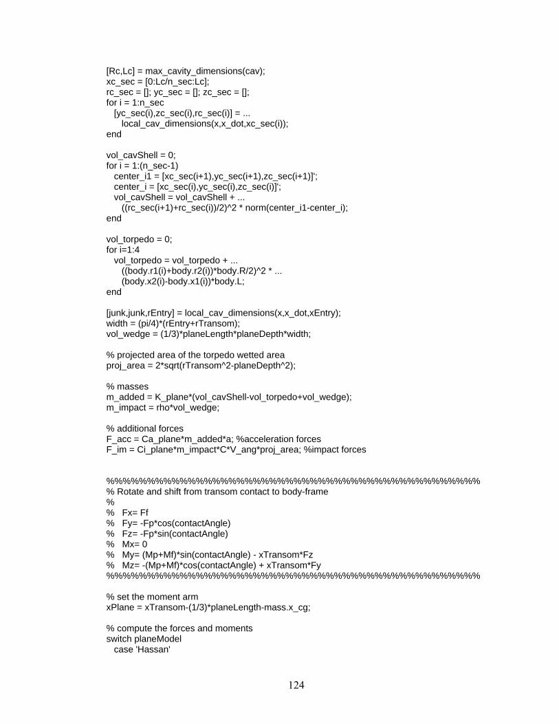
[Rc,Lc] = max_cavity_dimensions(cav); xc_sec = [0:Lc/n_sec:Lc]; rc_sec = []; yc_sec = []; zc_sec = []; for i = 1:n_sec [yc_sec(i),zc_sec(i),rc_sec(i)] = ... local_cav_dimensions(x,x_dot,xc_sec(i)); end vol_cavShell = 0; for i = 1:(n_sec-1) center_i1 = [xc_sec(i+1),yc_sec(i+1),zc_sec(i+1)]'; center_i = [xc_sec(i),yc_sec(i),zc_sec(i)]'; vol_cavShell = vol_cavShell + ... ((rc_sec(i+1)+rc_sec(i))/2)^2 * norm(center_i1-center_i); end vol_torpedo = 0; for i=1:4 vol_torpedo = vol_torpedo + ... ((body.r1(i)+body.r2(i))*body.R/2)^2 * ... (body.x2(i)-body.x1(i))*body.L; end [junk,junk,rEntry] = local_cav_dimensions(x,x_dot,xEntry); width = (pi/4)*(rEntry+rTransom); vol_wedge = (1/3)*planeLength*planeDepth*width; % projected area of the torpedo wetted area proj_area = 2*sqrt(rTransom^2-planeDepth^2); % masses m_added = K_plane*(vol_cavShell-vol_torpedo+vol_wedge); m_impact = rho*vol_wedge; % additional forces F_acc = Ca_plane*m_added*a; %acceleration forces F_im = Ci_plane*m_impact*C*V_ang*proj_area; %impact forces %%%%%%%%%%%%%%%%%%%%%%%%%%%%%%%%%%%%%%%%%%%%%% % Rotate and shift from transom contact to body-frame % % Fx= Ff % Fy= -Fp*cos(contactAngle) % Fz= -Fp*sin(contactAngle) % Mx= 0 % My= (Mp+Mf)*sin(contactAngle) - xTransom*Fz % Mz= -(Mp+Mf)*cos(contactAngle) + xTransom*Fy %%%%%%%%%%%%%%%%%%%%%%%%%%%%%%%%%%%%%%%%%%%%%% % set the moment arm xPlane = xTransom-(1/3)*planeLength-mass.x_cg; % compute the forces and moments switch planeModel case 'Hassan'

124

Fplane = [Ff, -Fp*cos(planeContact), -Fp*sin(planeContact) ]'; Mplane = [0, (Mp+Mf)*sin(planeContact), -(Mp+Mf)*cos(planeContact)]'; Mplane = Mplane + cross([mass.x_cg-xPlane,0,0]',Fplane); case 'Hassan_and_Song' Fplane = [Ff, -(Fp+F_acc+F_im)*cos(planeContact), ... -(Fp+F_acc+F_im)*sin(planeContact) ]'; Mplane = [0, (Mp+Mf)*sin(planeContact), -(Mp+Mf)*cos(planeContact)]'; Mplane = Mplane + cross([mass.x_cg-xPlane,0,0]',Fplane); otherwise disp('The planing forces were not computed') end %switch end %if ((hTransom > 0) & (body.planeSec(i) == 1)) out = [Fplane; Mplane]; return

125

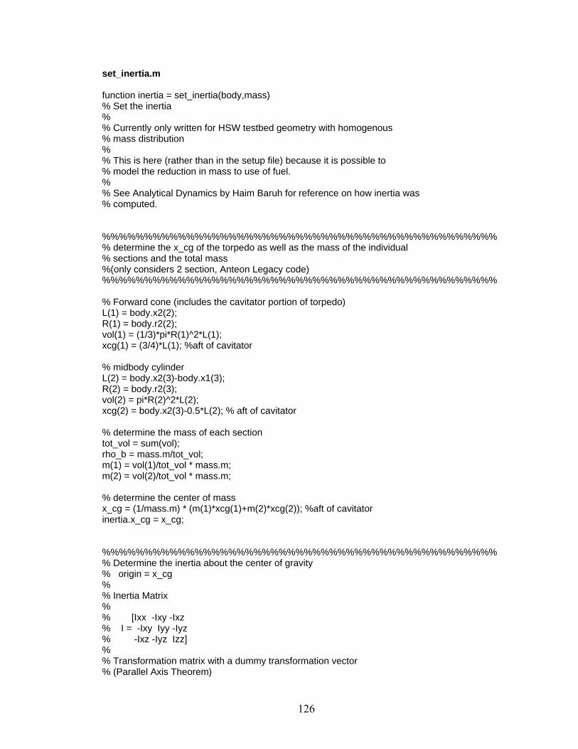
set_inertia.m function inertia = set_inertia(body,mass) % Set the inertia % % Currently only written for HSW testbed geometry with homogenous % mass distribution % % This is here (rather than in the setup file) because it is possible to % model the reduction in mass to use of fuel. % % See Analytical Dynamics by Haim Baruh for reference on how inertia was % computed. %%%%%%%%%%%%%%%%%%%%%%%%%%%%%%%%%%%%%%%%%%%%%%% % determine the x_cg of the torpedo as well as the mass of the individual % sections and the total mass %(only considers 2 section, Anteon Legacy code) %%%%%%%%%%%%%%%%%%%%%%%%%%%%%%%%%%%%%%%%%%%%%%% % Forward cone (includes the cavitator portion of torpedo) L(1) = body.x2(2); R(1) = body.r2(2); vol(1) = (1/3)*pi*R(1)^2*L(1); xcg(1) = (3/4)*L(1); %aft of cavitator % midbody cylinder L(2) = body.x2(3)-body.x1(3); R(2) = body.r2(3); vol(2) = pi*R(2)^2*L(2); xcg(2) = body.x2(3)-0.5*L(2); % aft of cavitator % determine the mass of each section tot_vol = sum(vol); rho_b = mass.m/tot_vol; m(1) = vol(1)/tot_vol * mass.m; m(2) = vol(2)/tot_vol * mass.m; % determine the center of mass x_cg = (1/mass.m) * (m(1)*xcg(1)+m(2)*xcg(2)); %aft of cavitator inertia.x_cg = x_cg; %%%%%%%%%%%%%%%%%%%%%%%%%%%%%%%%%%%%%%%%%%%%%%% % Determine the inertia about the center of gravity % origin = x_cg % % Inertia Matrix % % [Ixx -Ixy -Ixz % I = -Ixy Iyy -Iyz % -Ixz -Iyz Izz] % % Transformation matrix with a dummy transformation vector % (Parallel Axis Theorem)

126

% Tvec = [dx,dy,dz]; % Tmat = [ (dx^2+dy^2), -dx*dy, -dx*dz; % -dx*dy, (dx^2+dz^2), -dy*dz; % -dx*dz, -dy*dz, (dx^2+dy^2)]; % % such that I = Ig + m*Tmat %%%%%%%%%%%%%%%%%%%%%%%%%%%%%%%%%%%%%%%%%%%%%%% % calculate the inertia of the cone (about cone's cg) Iyy = (3/20)*m(1)*R(1)^2 + (3/80)*m(1)*L(1)^2; Izz = Iyy; Ixx = (3/10)*m(1)*R(1)^2; Icone = diag([Ixx,Iyy,Izz]); % Transform the cone inertia to the origin dx = xcg(1) - x_cg; dy = 0; dz = 0; Tmat = [ (dy^2+dz^2), -dx*dy, -dx*dz; -dx*dy, (dx^2+dz^2), -dy*dz; -dx*dz, -dy*dz, (dx^2+dy^2)]; Icone = Icone + m(1)*Tmat; % calculate the inertia of the cylinder (about cylinder's cg) Iyy = (1/4)*m(2)*R(2)^2 + (1/12)*m(2)*L(2)^2; Izz = Iyy; Ixx = (1/2)*m(2)*R(2)^2; Icyl = diag([Ixx,Iyy,Izz]); % Transform the cylinder inertia to the origin dx = xcg(2) - x_cg; dy = 0; dz = 0; Tmat = [ (dy^2+dz^2), -dx*dy, -dx*dz; -dx*dy, (dx^2+dz^2), -dy*dz; -dx*dz, -dy*dz, (dx^2+dy^2)]; Icyl = Icyl + m(2)*Tmat; % Compute the total angular inertia inertia.J = Icone + Icyl;

127

mass_forces.m function [out] = mass_forces(in) global mass body inertia % gravity forces and moments % set the input eul = in(1:3); %[phi,theta,psi]' vel = in(4:6); %[u,v,w]' omg = in(7:9); %[p,q,r]' phi = eul(1); theta = eul(2); psi = eul(3); % Define the transformation matrix to bring the gavity forces to body % forces c1 = cos(phi); c2= cos(theta); c3= cos(psi); s1 = sin(phi); s2= sin(theta); s3= sin(psi); T_i2b = [ c3*c2, -c1*s3+c3*s1*s2, s1*s3+c3*c1*s2 ; ... s3*c2, c1*c3+s3*s1*s2, -s1*c3+s3*c1*s2 ; ... -s2, s1*c2, c1*c2]; T_b2i = T_i2b'; % compute the gravity forces and moments Fgrav = T_b2i*[0,0,mass.m*mass.g]'; Mgrav = zeros(3,1); % set the output out = [Fgrav; Mgrav]; return

128

sixDofEom.m function [out] = sixDofEom(in) global sim hwait mass body inertia % define the input eul = in(1:3); %[phi,theta,psi] vel = in(4:6); %[u,v,w] omg = in(7:9); %[p,q,r] Fcav = in(10:12); Mcav = in(13:15); Ffin = in(16:18); Mfin = in(19:21); Fplane = in(22:24); Mplane = in(25:27); Fmass = in(28:30); Mmass = in(31:33); thrust = in(34:36); t = in(37); phi = eul(1); theta = eul(2); psi = eul(3); % update the waitbar if sim.simulating == true waitbar(t/sim.t_stop,hwait) end %%%%%%%%%%%%%%%%%%%%%%%%%%%%%%%%%%%%%%%%%%%%%%% % compute the kinematics %%%%%%%%%%%%%%%%%%%%%%%%%%%%%%%%%%%%%%%%%%%%%%% s1= sin(phi); c1= cos(phi); s2= sin(theta); c2= cos(theta); tan2= tan(theta); sec2= sec(theta); Tb2i_ang= [1, s1*tan2, c1*tan2 ; ... 0, c1, -s1 ; ... 0, s1*sec2, c1*sec2 ]; eul_dot = Tb2i_ang*omg; %%%%%%%%%%%%%%%%%%%%%%%%%%%%%%%%%%%%%%%%%%%%%%% % compute the dynamics % % NOTE: The dynamics equations assumes that the reference frame % being used is about the cg %%%%%%%%%%%%%%%%%%%%%%%%%%%%%%%%%%%%%%%%%%%%%%% % compute the moments produced by the thrust vector about the cg Mthrust = cross([body.L-mass.x_cg,0,0]',thrust); % compute the omega shorthand matrix p = omg(1); q = omg(2); r = omg(3); omg_tilde = [0,-r,q; r,0,-p; -q,p,0]; OMG = [-omg_tilde,zeros(3); zeros(3),-omg_tilde]; % compute the mass shorthand matrix M = [mass.m*eye(3),zeros(3); zeros(3),inertia.J];

129

% sum forces and moments about the cg Ftot = (Fmass+Fcav+Ffin+Fplane+thrust); Mtot = (Mmass+Mcav+Mfin+Mplane+Mthrust); % EOM accel = inv(M) * (OMG*M*[vel;omg] + [Ftot;Mtot]); vel_dot = accel(1:3); omg_dot = accel(4:6); % set the output out = [eul_dot; vel_dot; omg_dot];

130

body_immersion.m function [depth, angle] = body_immersion(x,x_dot,X,pSec,body) % This function calculates the torpedo body immersion % initialize output angle = 0; depth = 0; % calculate the slope of the body's radius x1 = body.x1(pSec); x2 = body.x2(pSec); r1 = body.r1(pSec); r2 = body.r2(pSec); Rb = (r1-r2)/(x1-x2)*(X-x2)+r2; % check that x is within body section if ((X > x2 | X < x1) & (X ~= x2) & (X ~= x1)) warning('Outside specified body section.'); return end % Interpolate cavity profile to find radius and center offset at chosen x % position (behind the cavitator) [yc,zc,rc] = local_cav_dimensions(x,x_dot,X); angle = pi + atan2(zc,yc); depth = Rb + (sqrt(yc^2+zc^2)-rc); return

131

cavity_info.m function [out] = cavity_info(r_vec,beta_dot_vec,V) global cavity % Calculate three sets of vectors representing the cavity centerline and % the local radii. These vectors will be used to interpret the local % cavity states at a given distance behind the cavitator. % define the x distance behind the cavitator xc(1) = 0; for i = 2:cavity.n xc(i) = xc(i-1)+cavity.dx; end % determine the sectional centerline offset and radii for i = 1:cavity.n x = [r_vec(i),0]; x_dot = [0,beta_dot_vec(i)]; [yc(i),zc(i),rc(i)] = local_cav_dimensions(x,x_dot,xc(i),V); end % define the output out = [xc, yc, zc, rc];

132

compute_alpha_beta.m function [alpha,beta] = compute_alpha_beta(vel) % compute alpha and beta as defined by Etkin (pg 10-11) u = vel(1); v = vel(2); w = vel(3); speed = norm(vel); alpha = atan2(w,u); beta = asin(v/speed); return;

133

compute_drag.m function drag = compute_drag(x,u,rho) % set the global variables global planeModel mass inertia body cav cavity DELTA % define the state derivatives x_dot = zeros(9,1); s1= sin(x(1)); c1= cos(x(1)); s2= sin(x(2)); c2= cos(x(2)); tan2= tan(x(2)); sec2= sec(x(2)); Tb2i_ang= [1, s1*tan2, c1*tan2 ; ... 0, c1, -s1 ; ... 0, s1*sec2, c1*sec2 ]; x_dot(1:3) = Tb2i_ang*x(7:9); % compute the cavitator forces and moments cav_FandM = cavitator_forces([x;u;rho]); Fcav_x = cav_FandM(1); % Check the fin forces fin_FandM = fin_forces([x;x_dot;u;rho]); Ffin_x = fin_FandM(1); % check planing forces plane_FandM = planing_forces([x;x_dot;rho]); Fplane_x = plane_FandM(1); % check mass moments and forces mass_FandM = mass_forces(x); Fmass_x = mass_FandM(1); % sum the forces to get the drag value drag = Fcav_x + Ffin_x + Fplane_x + Fmass_x;

134

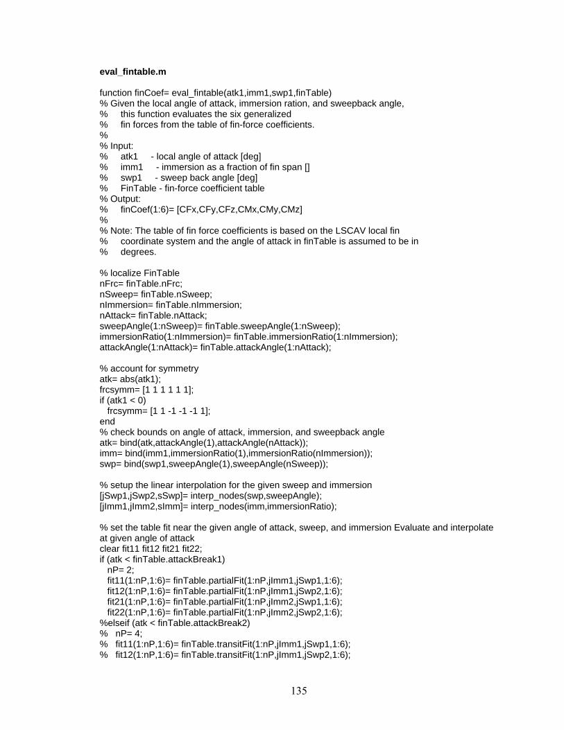
eval_fintable.m function finCoef= eval_fintable(atk1,imm1,swp1,finTable) % Given the local angle of attack, immersion ration, and sweepback angle, % this function evaluates the six generalized % fin forces from the table of fin-force coefficients. % % Input: % atk1 - local angle of attack [deg] % imm1 - immersion as a fraction of fin span [] % swp1 - sweep back angle [deg] % FinTable - fin-force coefficient table % Output: % finCoef(1:6)= [CFx,CFy,CFz,CMx,CMy,CMz] % % Note: The table of fin force coefficients is based on the LSCAV local fin % coordinate system and the angle of attack in finTable is assumed to be in % degrees. % localize FinTable nFrc= finTable.nFrc; nSweep= finTable.nSweep; nImmersion= finTable.nImmersion; nAttack= finTable.nAttack; sweepAngle(1:nSweep)= finTable.sweepAngle(1:nSweep); immersionRatio(1:nImmersion)= finTable.immersionRatio(1:nImmersion); attackAngle(1:nAttack)= finTable.attackAngle(1:nAttack); % account for symmetry atk= abs(atk1); frcsymm= [1 1 1 1 1 1]; if (atk1 < 0) frcsymm= [1 1 -1 -1 -1 1]; end % check bounds on angle of attack, immersion, and sweepback angle atk= bind(atk,attackAngle(1),attackAngle(nAttack)); imm= bind(imm1,immersionRatio(1),immersionRatio(nImmersion)); swp= bind(swp1,sweepAngle(1),sweepAngle(nSweep)); % setup the linear interpolation for the given sweep and immersion [jSwp1,jSwp2,sSwp]= interp_nodes(swp,sweepAngle); [jImm1,jImm2,sImm]= interp_nodes(imm,immersionRatio); % set the table fit near the given angle of attack, sweep, and immersion Evaluate and interpolate at given angle of attack clear fit11 fit12 fit21 fit22; if (atk < finTable.attackBreak1) nP= 2; fit11(1:nP,1:6)= finTable.partialFit(1:nP,jImm1,jSwp1,1:6); fit12(1:nP,1:6)= finTable.partialFit(1:nP,jImm1,jSwp2,1:6); fit21(1:nP,1:6)= finTable.partialFit(1:nP,jImm2,jSwp1,1:6); fit22(1:nP,1:6)= finTable.partialFit(1:nP,jImm2,jSwp2,1:6); %elseif (atk < finTable.attackBreak2) % nP= 4; % fit11(1:nP,1:6)= finTable.transitFit(1:nP,jImm1,jSwp1,1:6); % fit12(1:nP,1:6)= finTable.transitFit(1:nP,jImm1,jSwp2,1:6);

135

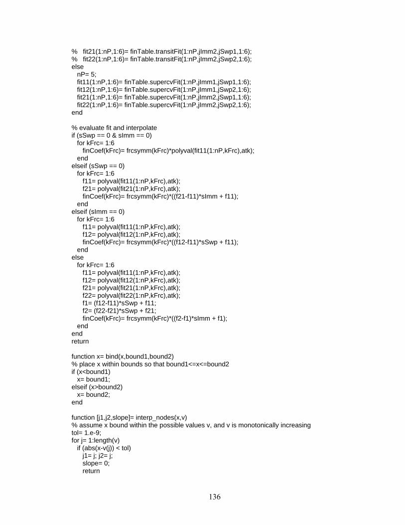
% fit21(1:nP,1:6)= finTable.transitFit(1:nP,jImm2,jSwp1,1:6); % fit22(1:nP,1:6)= finTable.transitFit(1:nP,jImm2,jSwp2,1:6); else nP= 5; fit11(1:nP,1:6)= finTable.supercvFit(1:nP,jImm1,jSwp1,1:6); fit12(1:nP,1:6)= finTable.supercvFit(1:nP,jImm1,jSwp2,1:6); fit21(1:nP,1:6)= finTable.supercvFit(1:nP,jImm2,jSwp1,1:6); fit22(1:nP,1:6)= finTable.supercvFit(1:nP,jImm2,jSwp2,1:6); end % evaluate fit and interpolate if (sSwp == 0 & sImm == 0) for kFrc= 1:6 finCoef(kFrc)= frcsymm(kFrc)*polyval(fit11(1:nP,kFrc),atk); end elseif (sSwp == 0) for kFrc= 1:6 f11= polyval(fit11(1:nP,kFrc),atk); f21= polyval(fit21(1:nP,kFrc),atk); finCoef(kFrc)= frcsymm(kFrc)*((f21-f11)*sImm + f11); end elseif (sImm == 0) for kFrc= 1:6 f11= polyval(fit11(1:nP,kFrc),atk); f12= polyval(fit12(1:nP,kFrc),atk); finCoef(kFrc)= frcsymm(kFrc)*((f12-f11)*sSwp + f11); end else for kFrc= 1:6 f11= polyval(fit11(1:nP,kFrc),atk); f12= polyval(fit12(1:nP,kFrc),atk); f21= polyval(fit21(1:nP,kFrc),atk); f22= polyval(fit22(1:nP,kFrc),atk); f1= (f12-f11)*sSwp + f11; f2= (f22-f21)*sSwp + f21; finCoef(kFrc)= frcsymm(kFrc)*((f2-f1)*sImm + f1); end end return function x= bind(x,bound1,bound2) % place x within bounds so that bound1<=x<=bound2 if (x<bound1) x= bound1; elseif (x>bound2) x= bound2; end function [j1,j2,slope]= interp_nodes(x,v) % assume x bound within the possible values v, and v is monotonically increasing tol= 1.e-9; for j= 1:length(v) if (abs(x-v(j)) < tol) j1= j; j2= j; slope= 0; return

136

end if (x < v(j)) j1= j-1; j2= j; delv= v(j2)-v(j1); if (abs(delv) < tol) slope= 0; return else slope= (x-v(j1))/delv; return end end end return

137

immersion_depth.m function immDepth = immersion_depth(x,states,states_dot,pSec,body) % function used in fzero to calculate the point of body immersion [immDepth,immAngle] = body_immersion(states,states_dot,x,pSec,body); return

138

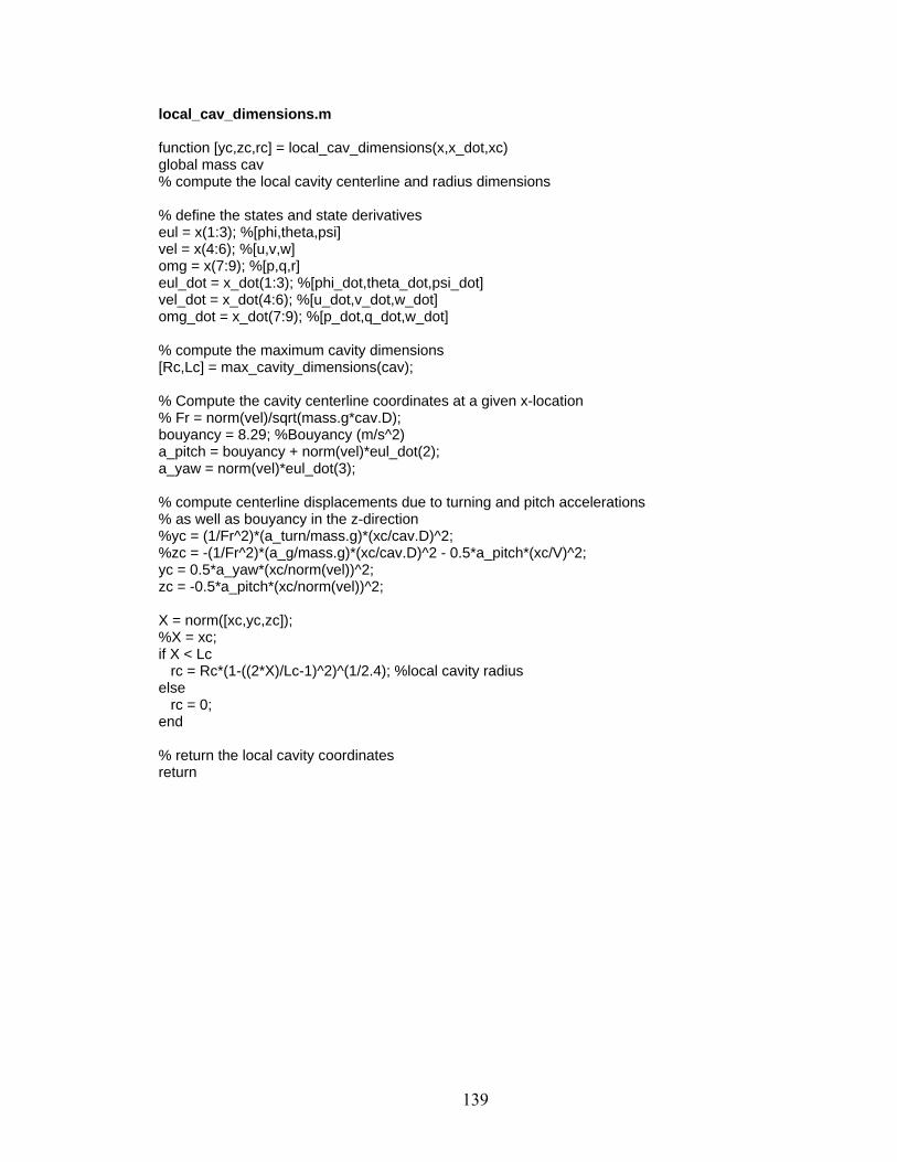
local_cav_dimensions.m function [yc,zc,rc] = local_cav_dimensions(x,x_dot,xc) global mass cav % compute the local cavity centerline and radius dimensions % define the states and state derivatives eul = x(1:3); %[phi,theta,psi] vel = x(4:6); %[u,v,w] omg = x(7:9); %[p,q,r] eul_dot = x_dot(1:3); %[phi_dot,theta_dot,psi_dot] vel_dot = x_dot(4:6); %[u_dot,v_dot,w_dot] omg_dot = x_dot(7:9); %[p_dot,q_dot,w_dot] % compute the maximum cavity dimensions [Rc,Lc] = max_cavity_dimensions(cav); % Compute the cavity centerline coordinates at a given x-location % Fr = norm(vel)/sqrt(mass.g*cav.D); bouyancy = 8.29; %Bouyancy (m/s^2) a_pitch = bouyancy + norm(vel)*eul_dot(2); a_yaw = norm(vel)*eul_dot(3); % compute centerline displacements due to turning and pitch accelerations % as well as bouyancy in the z-direction %yc = (1/Fr^2)*(a_turn/mass.g)*(xc/cav.D)^2; %zc = -(1/Fr^2)*(a_g/mass.g)*(xc/cav.D)^2 - 0.5*a_pitch*(xc/V)^2; yc = 0.5*a_yaw*(xc/norm(vel))^2; zc = -0.5*a_pitch*(xc/norm(vel))^2; X = norm([xc,yc,zc]); %X = xc; if X < Lc rc = Rc*(1-((2*X)/Lc-1)^2)^(1/2.4); %local cavity radius else rc = 0; end % return the local cavity coordinates return

139

make_comp_graphs.m % This function is designed to make state plots for two sets of data function [] = make_comp_graphs(t,x1,x2) % check for engineering zeros [row,col] = size(x1); tol = 1e-9; for i = 1:col if max(x1(:,i)) < tol x1(:,i) = zeros(row,1); end end [row,col] = size(x2); tol = 1e-9; for i = 1:col if max(x2(:,i)) < tol x2(:,i) = zeros(row,1); end end figure % phi subplot(3,3,1) plot(t,x1(:,1),'b-',t,x2(:,1),'r--') grid on ylabel('\phi (rad)') legend('Nonlinear','Linear') % theta subplot(3,3,4) plot(t,x1(:,2),'b-',t,x2(:,2),'r--') grid on ylabel('\theta (rad)') legend('Nonlinear','Linear') % psi subplot(3,3,7) plot(t,x1(:,3),'b-',t,x2(:,3),'r--') grid on ylabel('\psi (rad)') xlabel('Time (sec)') legend('Nonlinear','Linear') % u subplot(3,3,2) plot(t,x1(:,4),'b-',t,x2(:,4),'r--') grid on ylabel('u (m/s)') legend('Nonlinear','Linear') % v subplot(3,3,5) plot(t,x1(:,5),'b-',t,x2(:,5),'r--')

140

grid on ylabel('v (m/s)') legend('Nonlinear','Linear') % z subplot(3,3,8) plot(t,x1(:,6),'b-',t,x2(:,6),'r--') grid on ylabel('z (m/s)') xlabel('Time (sec)') legend('Nonlinear','Linear') % p subplot(3,3,3) plot(t,x1(:,7),'b-',t,x2(:,7),'r--') grid on ylabel('p (rad/sec)') legend('Nonlinear','Linear') % q subplot(3,3,6) plot(t,x1(:,8),'b-',t,x2(:,8),'r--') grid on ylabel('q (rad/sec)') legend('Nonlinear','Linear') % r subplot(3,3,9) plot(t,x1(:,9),'b-',t,x2(:,9),'r--') grid on ylabel('r (rad/sec)') xlabel('Time (sec)') legend('Nonlinear','Linear')

141

make_graphs.m % This function is designed to make state plots function [] = make_graphs(t,x) % check for engineering zeros [row,col] = size(x); tol = 1e-9; for i = 1:col if max(x(:,i)) < tol x(:,i) = zeros(row,1); end end figure % phi subplot(3,3,1) plot(t,x(:,1)) grid on ylabel('\phi (rad)') % theta subplot(3,3,4) plot(t,x(:,2)) grid on ylabel('\theta (rad)') % psi subplot(3,3,7) plot(t,x(:,3)) grid on ylabel('\psi (rad)') xlabel('Time (sec)') % u subplot(3,3,2) plot(t,x(:,4)) grid on ylabel('u (m/s)') % v subplot(3,3,5) plot(t,x(:,5)) grid on ylabel('v (m/s)') % z subplot(3,3,8) plot(t,x(:,6)) grid on ylabel('z (m/s)') xlabel('Time (sec)') % p subplot(3,3,3)

142

plot(t,x(:,7)) grid on ylabel('p (rad/sec)') % q subplot(3,3,6) plot(t,x(:,8)) grid on ylabel('q (rad/sec)') % r subplot(3,3,9) plot(t,x(:,9)) grid on ylabel('r (rad/sec)') xlabel('Time (sec)')

143

max_cavity_dimensions.m function [Rc,Lc] = max_cavity_dimensions(cav) global DELTA % This function computes the maximum cavity dimensions % % Since there is no model for the cavitation number and assuming that the % drag coefficient remains constant, the maximum cavity dimensions are not % only not a function of the states, but remain constant % add the DELTA values Cd0 = cav.Cd0 + cav.Cd0*DELTA.Cd0_range(DELTA.Cd0_rval); sigma = cav.sigma + cav.sigma*DELTA.sigma_range(DELTA.sigma_rval); % Compute the maximum cavity dimensions Cd = Cd0*(1+sigma+0.028*sigma^2); %Drag Coefficient Lc = cav.D*sqrt(Cd)*(1.24*sigma^(-1.123)-0.6); %Maximum cavity length Rc = cav.R*sqrt(1.35*Cd*sigma^(-0.93)); %Maximum cavity radius return

144

scav_least_squares3.m % Determine the coefficients a, b, and c ( z(i,j) = a*x(i)+b*y(j)+c ) function [coef,normed_error] = scav_least_squares3(x,y,z) N = length(x); M = length(y); % Fill the A and B matrics A = zeros(N*M,3); B = zeros(N*M,1); for i = 1:N for j = 1:M A(M*(i-1)+j,:) = [x(i),y(j),1]; B(M*(i-1)+j) = z(i,j); end end coef = inv([A'*A])*A'*B; normed_error = norm(A*coef-B)/norm(B); return scav_least_squares6.m % Determine the coefficients [p1,p2,p3,p4,5p,p6] % z(i,j) = p1*x^2 + p2*x*y + p3*y^2 + p4*x + p5*y + p6 function [coef,normed_error] = scav_least_squares6(x,y,z) N = length(x); M = length(y); % Fill the A and B matrics A = zeros(N*M,6); B = zeros(N*M,1); for i = 1:N for j = 1:M A(M*(i-1)+j,:) = [x(i)^2, x(i)*y(j), y(j)^2, x(i), y(j), 1]; B(M*(i-1)+j) = z(i,j); end end coef = inv([A'*A])*A'*B; normed_error = norm(A*coef-B)/norm(B); return scav_least_squares8.m % Determine the coefficients [p1,p2,p3,p4,p5,p6,97,p8] % z(i,j) = p1*x^3 + p2*y^3 + p3*x^2*y + p4*x*y^2 + p5*x*y + p6*x + p7*y + % p8 function [coef,normed_error] = scav_least_squares8(x,y,z) N = length(x); M = length(y); % Fill the A and B matrics

145

A = zeros(N*M,8); B = zeros(N*M,1); for i = 1:N for j = 1:M A(M*(i-1)+j,:) = [x(i)^3, y(j)^3, x(i)^2*y(j), x(i)*y(j)^2,... x(i)*y(j), x(i), y(j), 1]; B(M*(i-1)+j) = z(i,j); end end coef = inv([A'*A])*A'*B; normed_error = norm(A*coef-B)/norm(B); return

146

test_ol_sensitivity.m % This function is designed to test the open sensitivity to variations in % system parameters as is defined in setup_sim_data. It does this by % comparing the A and B matrices as well as comparing stability % set the global variables global planeModel mass inertia body cav cavity DELTA global sim hwait % set constants and model data [mass, inertia, body, cav, cavity, rho] = setup_sim_data; %%%%%%%%%%%%%%%%%%%%%%%%%%%%%%%%%%%%%%%%%%%%%%% % Setup simulation parameters %%%%%%%%%%%%%%%%%%%%%%%%%%%%%%%%%%%%%%%%%%%%%%% sim.dt = 0.001; %sec sim.t_stop = 2; %sec sim.simulating = false; % set the nominal speed V = 82.25; % set the turning acceleration turnG = 0; % set the flight condition: % 'straight-and-level' % 'turn' flight_con = 'straight-and-level'; %flight_con = 'turn'; % set the initial heading initial_heading = 0; % set the output reference frame and appropriate transformation matrix mass.origin_method = 'U of MN'; %('U of MN','Anteon') switch mass.origin_method case 'U of MN' dist = [0;0;0]; case 'Anteon' dist = [mass.x_cg;0;0]'; otherwise error('Incorrect origin setting') end r_tilde = [0,-dist(3),dist(2); dist(3),0,-dist(1); -dist(2),dist(1),0]; R = [eye(3),r_tilde; zeros(3),eye(3)]; % define value for uncertainty ranges minVal = 1; nomVal = 2; maxVal = 3;

147

%%%%%%%%%%%%%%%%%%%%%%%%%%%%%%%%%%%%%%%%%%%%%%% % Define Initial/Trim Conditions %%%%%%%%%%%%%%%%%%%%%%%%%%%%%%%%%%%%%%%%%%%%%%% % set the planing model (no planing is desired) planeModel = 'Hassan'; % set the appropraite trim conditions switch flight_con case 'straight-and-level' x0 = [0,0,initial_heading,V,0,0,0,0,0]'; thrust = -1*compute_drag(x0,zeros(6,1),rho); u0 = [0,0,0,0,0,0,thrust,0,0]'; [x0,u0,y0,dx,options] = trim('trim_6DOF_model',x0,u0,[],... [1,2,3,4,5,6,7,8,9],[2,4,6,8,9]); case 'turn' x0 = [0,0,initial_heading,V,0,0,0,0,(turnG*9.81)/V]'; x_dot = zeros(9,1); s1= sin(x0(1)); c1= cos(x0(1)); s2= sin(x0(2)); c2= cos(x0(2)); tan2= tan(x0(2)); sec2= sec(x0(2)); Tb2i_ang= [1, s1*tan2, c1*tan2 ; ... 0, c1, -s1 ; ... 0, s1*sec2, c1*sec2 ]; x_dot(1:3) = Tb2i_ang*x0(7:9); x_dot(1) = 0; thrust = -1*compute_drag(x0,zeros(6,1),rho); u0 = [0,0,0,0,0,0,thrust,0,0]'; [x0,u0,y0,dx,options] = trim('trim_6DOF_model',x0,u0,[],... [9],[8,9],[],x_dot,[1,2,3,4,5,6,7,8,9]); otherwise disp('Incorrect flight condition setting') return end % check for engineering zeros in x0 and u0 tol = 1e-9; for i = 1:length(x0) if abs(x0(i)) < tol x0(i) = 0; end end for i = 1:length(u0) if abs(u0(i)) < tol u0(i) = 0; end end % display the trim conditions disp(' ') disp('The trim conditions are as follows:') disp(' x0 u0 y0 dx0') disp([x0,u0,y0,dx]) % set the initial conditions thrust = u0(7:9); u0 = u0(1:6);

148

x0 = x0; %%%%%%%%%%%%%%%%%%%%%%%%%%%%%%%%%%%%%%%%%%%%%%% % Compute the Nominal Linearized Model %%%%%%%%%%%%%%%%%%%%%%%%%%%%%%%%%%%%%%%%%%%%%%% input_step_matrix = zeros(6,6); state_step_matrix = zeros(9,9); planeModel = 'Hassan'; [A_nom,B_nom,C_nom,D_nom] = linmod('ol_model'); nom_sys = ss(A_nom,B_nom,C_nom,D_nom); %%%%%%%%%%%%%%%%%%%%%%%%%%%%%%%%%%%%%%%%%%%%%%% % Check the sensitivity to the fin force and moment coefficients %%%%%%%%%%%%%%%%%%%%%%%%%%%%%%%%%%%%%%%%%%%%%%% for coef = 1:6 DELTA.Cfin_coef = coef; % compute the linear system with the min parameter DELTA.Cfin_rval = minVal; [A_min,B_min,C_min,D_min] = linmod('ol_model'); min_sys = ss(A_min,B_min,C_min,D_min); % compute the linear system with the max parameter DELTA.Cfin_rval = maxVal; [A_max,B_max,C_max,D_max] = linmod('ol_model'); max_sys = ss(A_max,B_max,C_max,D_max); % reset to the nominal value DELTA.Cfin_rval = nomVal; % make the varying system pole-zero map figure pzmap(nom_sys,'k',min_sys,'r',max_sys,'b') grid on legend('Nominal','Minimum','Maximum') title(['Open-Loop Pole-Zero Map for Fin Coefficient Index ',num2str(coef)]) end %%%%%%%%%%%%%%%%%%%%%%%%%%%%%%%%%%%%%%%%%%%%%%% % Check the sensitivity to the cavitator Cd0 %%%%%%%%%%%%%%%%%%%%%%%%%%%%%%%%%%%%%%%%%%%%%%% % compute the linear system with the min parameter DELTA.Cd0_rval = minVal; [A_min,B_min,C_min,D_min] = linmod('ol_model'); min_sys = ss(A_min,B_min,C_min,D_min); % compute the linear system with the max parameter DELTA.Cd0_rval = maxVal; [A_max,B_max,C_max,D_max] = linmod('ol_model');

149

max_sys = ss(A_max,B_max,C_max,D_max); % reset to the nominal value DELTA.Cd0_rval = nomVal; % make the varying system pole-zero map figure pzmap(nom_sys,'k',min_sys,'r',max_sys,'b') grid on legend('Nominal','Minimum','Maximum') title('Open-Loop Pole-Zero Map for Cd_0') %%%%%%%%%%%%%%%%%%%%%%%%%%%%%%%%%%%%%%%%%%%%%%% % Check the sensitivity to the cavitator number %%%%%%%%%%%%%%%%%%%%%%%%%%%%%%%%%%%%%%%%%%%%%%% % compute the linear system with the min parameter DELTA.sigma_rval = minVal; [A_min,B_min,C_min,D_min] = linmod('ol_model'); min_sys = ss(A_min,B_min,C_min,D_min); % compute the linear system with the max parameter DELTA.sigma_rval = maxVal; [A_max,B_max,C_max,D_max] = linmod('ol_model'); max_sys = ss(A_max,B_max,C_max,D_max); % reset to the nominal value DELTA.sigma_rval = nomVal; % make the varying system pole-zero map figure pzmap(nom_sys,'k',min_sys,'r',max_sys,'b') grid on legend('Nominal','Minimum','Maximum') title('Open-Loop Pole-Zero Map for \sigma parameter')

150

test_turnG.m function [maxG] = test_turnG(Vrange) % The purpose of this function is to test the min and max allowable turnG % before planing forces occur. Keep in mind that planing forces are not % desirable and that the limit of the trajectory profile is based on the % occurance of these planing forces % set constants and model data [mass, inertia, body, cav, cavity, rho] = setup_sim_data; sim.dt = 0.001; %sec sim.t_stop = 0.5; %sec sim.simulating = false; initial_heading = 0; delG = 0.1; pSec = 3; % check max turnG for range of velocities maxG = zeros(1,length(Vrange)); for vel_index = 1:length(Vrange) % stop when planing occurs hTransom = -100; count = 0; turnG = 0; while (hTransom < 0) & (count < 100) %%%%%%%%%%%%%%%%%%%%%%%%%%%%%%%%%%%%%%%%%%%%% % Setup simulation parameters %%%%%%%%%%%%%%%%%%%%%%%%%%%%%%%%%%%%%%%%%%%%% % set the nominal speed V = Vrange(vel_index); % set the flight condition: % 'straight-and-level' % 'turn' %flight_con = 'straight-and-level'; flight_con = 'turn'; % set the output reference frame and appropriate transformation matrix mass.origin_method = 'U of MN'; %('U of MN','Anteon') switch mass.origin_method case 'U of MN' dist = [0;0;0]; case 'Anteon' dist = [mass.x_cg;0;0]'; otherwise error('Incorrect origin setting') end r_tilde = [0,-dist(3),dist(2); dist(3),0,-dist(1); -dist(2),dist(1),0]; R = [eye(3),r_tilde; zeros(3),eye(3)];

151

%%%%%%%%%%%%%%%%%%%%%%%%%%%%%%%%%%%%%%%%%%%%% % Define Initial/Trim Conditions %%%%%%%%%%%%%%%%%%%%%%%%%%%%%%%%%%%%%%%%%%%%% % set the planing model (no planing is desired) planeModel = 'Hassan'; % set the appropraite trim conditions x_dot = zeros(9,1); switch flight_con case 'straight-and-level' x0 = [0,0,initial_heading,V,0,0,0,0,0]'; thrust = -1*compute_drag(x0,zeros(6,1),rho); u0 = [0,0,0,0,0,0,thrust,0,0]'; [x0,u0,y0,dx,options] = trim('trim_6DOF_model',x0,u0,[],... [1,2,3,4,5,6,7,8,9],[2,4,6,8,9]); case 'turn' x0 = [0,0,initial_heading,V,0,0,0,0,(turnG*9.81)/V]'; x_dot = zeros(9,1); s1= sin(x0(1)); c1= cos(x0(1)); s2= sin(x0(2)); c2= cos(x0(2)); tan2= tan(x0(2)); sec2= sec(x0(2)); Tb2i_ang= [1, s1*tan2, c1*tan2 ; ... 0, c1, -s1 ; ... 0, s1*sec2, c1*sec2 ]; x_dot(1:3) = Tb2i_ang*x0(7:9); x_dot(1) = 0; thrust = -1*compute_drag(x0,zeros(6,1),rho); u0 = [0,0,0,0,0,0,thrust,0,0]'; [x0,u0,y0,dx,options] = trim('trim_6DOF_model',x0,u0,[],... [9],[8,9],[],x_dot,[1,2,3,4,5,6,7,8,9]); otherwise disp('Incorrect flight condition setting') return end % check for engineering zeros in x0 and u0 tol = 1e-9; for i = 1:length(x0) if abs(x0(i)) < tol x0(i) = 0; end end for i = 1:length(u0) if abs(u0(i)) < tol u0(i) = 0; end end % set the initial conditions thrust = u0(7:9); u = u0(1:6); x = x0; % define transom position and determine immersion there xTransom = body.x2(pSec); planeLength = 0;

152

[hTransom,aTransom] = body_immersion(x,x_dot,xTransom,pSec,body); % store max turnG value if hTransom > 0 maxG(vel_index) = turnG else turnG = turnG + delG; end count = count + 1 end %while end %for

153

Appendix C This appendix shows how the system dynamics vary with velocity.

154

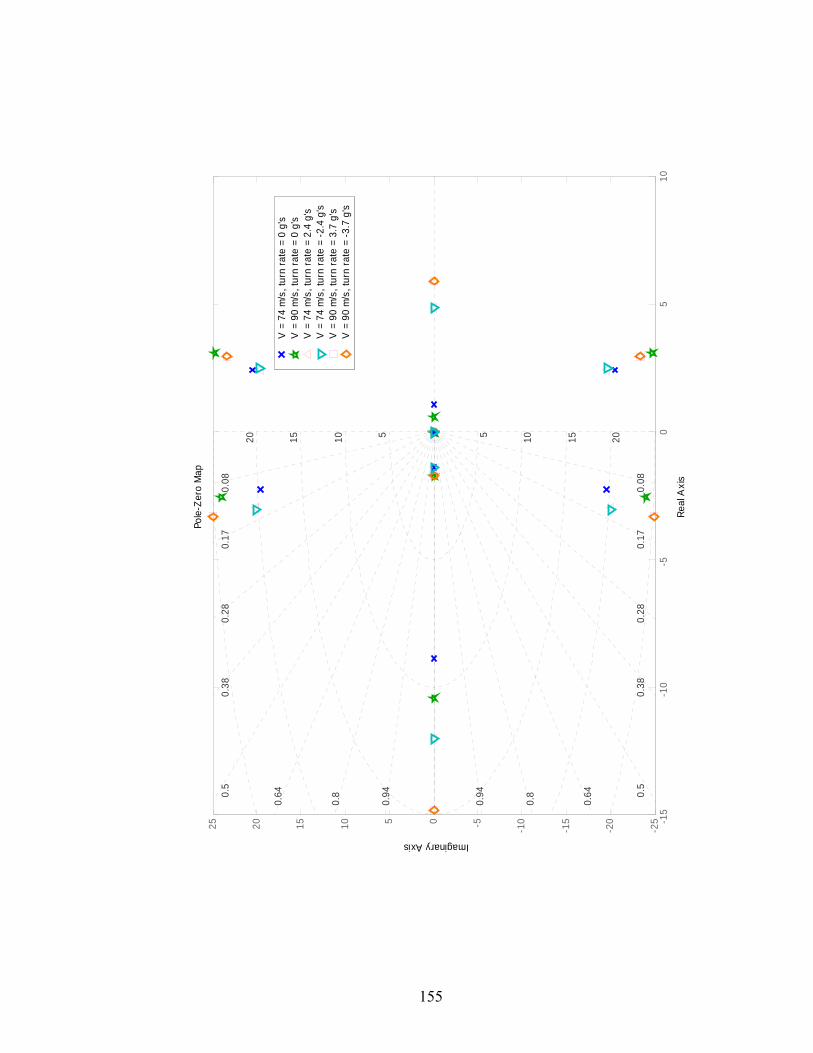
10

155

-15

-10

-50

5-2

5

-20

-15

-10-50510152025

0.38

0.28

0.17

0.08

0.94

0.8

0.640.

5

0.38

0.17

0.08

15

0.28

0.5

5 20

0.64

20 1015 105

0.8

0.94

V =

74

m/s

, tur

n ra

te =

0 g

'sV

= 9

0 m

/s, t

urn

rate

= 0

g's

V =

74

m/s

, tur

n ra

te =

2.4

g's

V =

74

m/s

, tur

n ra

te =

-2.4

g's

V =

90

m/s

, tur

n ra

te =

3.7

g's

V =

90

m/s

, tur

n ra

te =

-3.7

g's

Pole

-Zer

o M

ap

Real

Axi

s

Imaginary Axis

11 Appendix D This appendix displays pole-zero maps of the open-loop system for varying parameters. Given the range of the varying parameters, how the system dynamics change can be read from the graphs. The parameters shown here are the cavitation number, the cavitator drag coefficient and zero a.o.a., and the six fin force and moment coefficients.

156

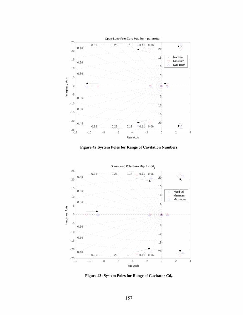
-12 -10 -8 -6 -4 -2 0 2 4-25

-20

-15

-10

-5

0

5

10

15

20

25

0.66

0.480.36 0.26 0.18 0.11 0.06

0.36 0.26 0.18 0.11 0.06

0.86 5

0.66

0.48

15

20

0.86

15

10

10

20

5

NominalMinimumMaximum

Open-Loop Pole-Zero Map for σ parameter

Real Axis

Imag

inar

y Ax

is

Figure 42:System Poles for Range of Cavitation Numbers

-12 -10 -8 -6 -4 -2 0 2 4-25

-20

-15

-10

-5

0

5

10

15

20

25

0.66

0.480.36 0.26 0.18 0.11 0.06

0.36 0.26 0.18 0.11 0.06

0.86 5

0.66

0.48

15

20

0.86

15

10

10

20

5

NominalMinimumMaximum

Open-Loop Pole-Zero Map for Cd0

Real Axis

Imag

inar

y Ax

is

Figure 43: System Poles for Range of Cavitator Cd0

157

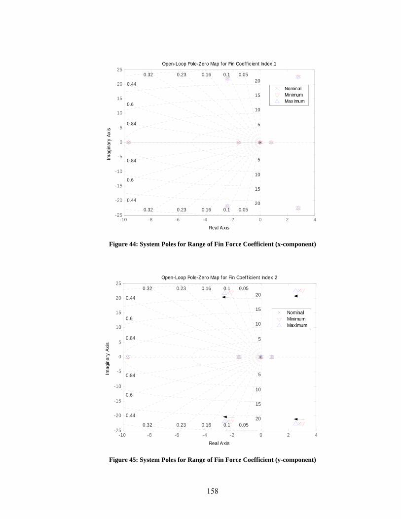
-10 -8 -6 -4 -2 0 2 4-25

-20

-15

-10

-5

0

5

10

15

20

25

0.6

0.44

0.32 0.23 0.16 0.1 0.05

0.32 0.23 0.16 0.1 0.05

0.84 5

0.6

0.44

15

20

0.84

15

10

10

20

5

NominalMinimumMaximum

Open-Loop Pole-Zero Map for Fin Coef f icient Index 1

Real Axis

Imag

inar

y Ax

is

Figure 44: System Poles for Range of Fin Force Coefficient (x-component)

-10 -8 -6 -4 -2 0 2 4-25

-20

-15

-10

-5

0

5

10

15

20

25

0.6

0.44

0.32 0.23 0.16 0.1 0.05

0.32 0.23 0.16 0.1 0.05

0.84 5

0.6

0.44

15

20

0.84

15

10

10

20

5

NominalMinimumMaximum

Open-Loop Pole-Zero Map for Fin Coef f icient Index 2

Real Axis

Imag

inar

y Ax

is

Figure 45: System Poles for Range of Fin Force Coefficient (y-component)

158

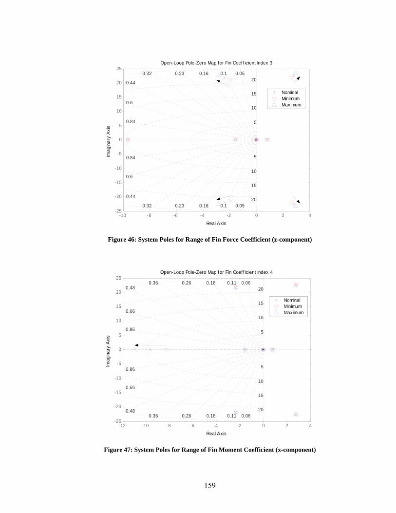
-10 -8 -6 -4 -2 0 2 4-25

-20

-15

-10

-5

0

5

10

15

20

25

0.6

0.44

0.32 0.23 0.16 0.1 0.05

0.32 0.23 0.16 0.1 0.05

0.84 5

0.6

0.44

15

20

0.84

15

10

10

20

5

NominalMinimumMaximum

Open-Loop Pole-Zero Map for Fin Coef f icient Index 3

Real Axis

Imag

inar

y Ax

is

Figure 46: System Poles for Range of Fin Force Coefficient (z-component)

-12 -10 -8 -6 -4 -2 0 2 4-25

-20

-15

-10

-5

0

5

10

15

20

25

0.66

0.480.36 0.26 0.18 0.11 0.06

0.36 0.26 0.18 0.11 0.06

0.86 5

0.66

0.48

15

20

0.86

15

10

10

20

5

NominalMinimumMaximum

Open-Loop Pole-Zero Map for Fin Coef f icient Index 4

Real Axis

Imag

inar

y Ax

is

Figure 47: System Poles for Range of Fin Moment Coefficient (x-component)

159

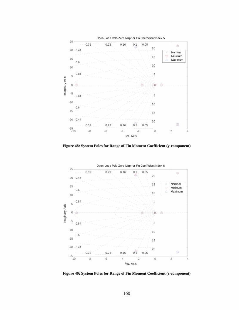
-10 -8 -6 -4 -2 0 2 4-25

-20

-15

-10

-5

0

5

10

15

20

25

0.6

0.44

0.32 0.23 0.16 0.1 0.05

0.32 0.23 0.16 0.1 0.05

0.84 5

0.6

0.44

15

20

0.84

15

10

10

20

5

NominalMinimumMaximum

Open-Loop Pole-Zero Map for Fin Coef f icient Index 5

Real Axis

Imag

inar

y Ax

is

Figure 48: System Poles for Range of Fin Moment Coefficient (y-component)

-10 -8 -6 -4 -2 0 2 4-25

-20

-15

-10

-5

0

5

10

15

20

25

0.6

0.44

0.32 0.23 0.16 0.1 0.05

0.32 0.23 0.16 0.1 0.05

0.84 5

0.6

0.44

15

20

0.84

15

10

10

20

5

NominalMinimumMaximum

Open-Loop Pole-Zero Map for Fin Coef f icient Index 6

Real Axis

Imag

inar

y Ax

is

Figure 49: System Poles for Range of Fin Moment Coefficient (z-component)

160