MULTIPHASE CFD MODELING OF DEVELOPED AND SUPERCAVITATING FLOWS

Robert F. KunzJules W. LindauMichael L. Billet

David R. StinebringApplied Research Laboratory

PO Box 30State College, PA 16804

USA

ABSTRACT ratio and the local volume fraction, which renders

Engineering interest in natural and ventilated cavi-ties about submerged bodies and in turbomachineryhas led researchers to study and attempt to modellarge scale cavitation for decades. Comparativelysimple analytical methods have been used widelyand successfully to model developed cavitation,since the hydrodynamics of these flows are oftendominated by irrotational and rotational inviscideffects. However, a range of more complex physicalphenomena are often associated with such cavities,including viscous effects, unsteadiness, mass trans-fer, three-dimensionality and compressibility.Though some of these complicating physics can beaccommodated in simpler physical models, theongoing maturation and increased generality of mul-tiphase Computational Fluid Dynamic (CFD) meth-ods has motivated recent research by a number ofgroups in the application of these methods for devel-oped cavitation analysis. This paper focuses on theauthors’ recent research activities in this area.

The authors have developed an implicit algorithmfor the computation of viscous two-phase flows. Thebaseline differential equation system is the multi-phase Navier-Stokes equations, comprised of themixture volume, mixture momentum and constitu-ent volume fraction equations. Though further gen-eralization is straightforward, a three-speciesformulation is pursued here, which separatelyaccounts for the liquid and vapor (which exchangemass) as well as a non-condensable gas field. Theimplicit method developed employs a dual-time,preconditioned, three-dimensional algorithm, withmulti-block and parallel execution capabilities.Time-derivative preconditioning is employed toensure well-conditioned eigenvalues, which isimportant for the computational efficiency of themethod. Special care is taken to ensure that theresulting eigensystem is independent of the density

1

the scheme well-suited to high density ratio, largelyphase-separated two-phase flows characteristic ofdeveloped and supercavitating systems. A dual-timeformulation is employed to accommodate the inher-ently unsteady physics of developed and super-cavi-ties. We have recently extended the formulation forcompressible constituents to accommodate analysisof high speed projectiles and rocket plumes, andthese formulation elements are also summarized. Todemonstrate the validation status and general capa-bilities of the scheme, numerous examples are pre-sented.

NOMENCLATURE

SymbolsAj flux JacobiansCµ, C1, C2 turbulence model constantsCdest, Cprod mass transfer model constantsCi pseudo-sound speedCP pressure coefficientCD drag coefficientD source Jacobiand body diameterdm bubble diametere total energy per unit volumeE, F, G flux vectorsf frequencygi gravity vectorh enthalpyH source vectorI identity matrixJ metric JacobianKj transform matrixk turbulent kinetic energyL bubble lengthM, Mj Mach number, similarity transform matrices

, mass transfer ratesP turbulent kinetic energy productionPrtk,Prtε turbulent Prandtl numbers for k and εp pressureQ transport variable vectorRe Reynolds numberStr Strouhal numbers arc length along configuration

time coordinate, mean flow time scale ( )Uj velocity magnitude, contravariant velocity com-ponentsui, u, v, w Cartesian velocity componentsxi Cartesian coordinates

m·-

m·+

t t∞, d/U∞

Y mass fractionα volume fraction, angle-of-attackβ preconditioning parameterΓ, Γe time derivative preconditioning and transformmatricesε turbulence dissipation rate, numerical Jacobian

parameter, internal energy per unit massκ, φ MUSCL parametersΛj, λj eigenvaluesµ molecular viscosityρ densityσ cavitation numberτ pseudo-time coordinateν dissipation sensorξj curvilinear coordinates

Subscripts, Superscripts1φ single-phase valuei, j coordinate indicesk constituent index, pseudo-time-step indexL, R dependent variable values on left and right offacel liquidm mixtureng non-condensable gast turbulentv condensable vapor, viscous

free stream valuetransformed to curvilinear coordinates

+/- production/destruction, right/left running~ with respect to mixtureY mass fraction form

INTRODUCTION

Multi-phase flows have received growing researchattention among CFD practitioners due in large mea-sure to the evolving maturity of single-phase algo-rithms that have been adapted to the increasedcomplexity of multi-component systems. However,there remain a number of numerical and physicalmodeling challenges that arise in multi-phase CFDanalysis beyond those present in single-phase meth-ods. Principal among these are large constituent den-sity ratios, the presence of discrete interfaces,significant mass transfer rates, non-equilibriuminterfacial dynamics, compressibility effects associ-ated with the very low mixture sound speeds whichcan arise, the presence of multiple constituents (viz.more than two) and void wave propagation. Thesenaturally deserve special attention when a numericalmethod is constructed or adapted for multi-phaseflows.

The class of multiphase flows under considerationhere is developed- and super-cavitating flows,wherein significant regions of the flow are occupiedby gas phase. Depending on the configuration, such“developed” [38] cavities are composed of vaporand/or injected non-condensable gas.

Historically, most efforts to model large cavitiesrelied on potential flow methods applied to the liq-

uid flow, while the bubble shape and closure condi-tions were specified. Adaptations of potential flowmethods remain in widespread use today ([15]), dueto their inherent computational efficiency, and theirproven effectiveness in predicting numerous firstorder dynamics of supercavitating configurations.

Recently, more general CFD approaches have beendeveloped to analyze these flows. In one class ofmethods, a single continuity equation is consideredwith the density varying abruptly between vapor andliquid densities through an equation of state. Such“single-continuity-equation-homogeneous” methodshave become fairly widely used for sheet and super-cavitation analysis ([8], [9], [25], [35], [43], forexample). Although these methods can directlymodel viscous effects, they are inherently unable todistinguish between condensable vapor and non-condensable gas, a requirement of ventilated super-cavitating vehicle analysis.

By solving separate continuity equations for liquidand gas phase fields, one can account for and modelthe separate dynamics and thermodynamics of theliquid, condensable vapor, and non-condensable gasfields. Such multi-species methods are also termedhomogeneous because interfacial dynamics areneglected, that is, there is assumed to be no-slipbetween constituents residing in the same controlvolume. A number of researchers have adopted thislevel of differential modeling, mostly for the analy-sis of natural cavitation where two phases/constitu-ents are accounted for ([1], [23], [32], for example).This is the level of modeling employed here, thougha three-species formulation is used to account fortwo gaseous fields. For two phases/constituentsthese methods are very closely related to the“single-continuity-equation-homogeneous” methodsaddressed above with interfacial mass transfer mod-eling supplanting an equation of state.

Full-two-fluid modeling, wherein separate momen-tum (and in principle energy) equations areemployed for the liquid and vapor constituents, havealso been utilized for natural cavitation (Groggerand Alajbegovic [12]). However, in sheet-cavityflows, the gas-liquid interface is known to be nearlyin dynamic equilibrium; for this reason, we do notpursue a full two-fluid level of modeling.

Sheet- and super-cavitating flows are characterizedby large density ratios (ρl/ρv > 104 is observed innear-atmospheric water applications), relatively dis-

∞

2

crete cavity-free stream interfaces and, due to venti-lation, multiple gas phase constituents. Accordingly,the CFD method employed must accommodatethese physics effectively.

Most relevant applications exhibit large scaleunsteadiness associated with re-entrant jets, periodicejection of non-condensable gas, and cavity “pulsa-tions”. Accordingly, we and others ([23], [26], [32],[35], for example) employ a time-accurate formula-tion in the analysis of large scale cavitation.

Compressibility

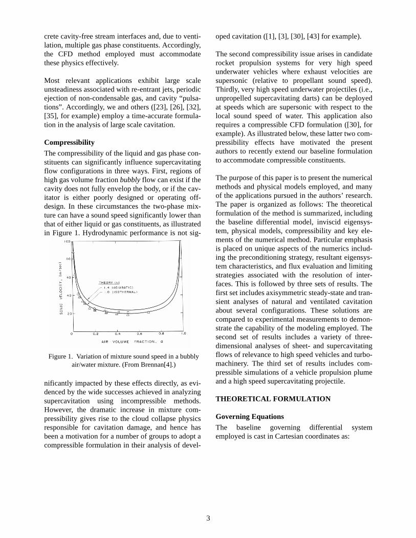
The compressibility of the liquid and gas phase con-stituents can significantly influence supercavitatingflow configurations in three ways. First, regions ofhigh gas volume fraction bubbly flow can exist if thecavity does not fully envelop the body, or if the cav-itator is either poorly designed or operating off-design. In these circumstances the two-phase mix-ture can have a sound speed significantly lower thanthat of either liquid or gas constituents, as illustratedin Figure 1. Hydrodynamic performance is not sig-

nificantly impacted by these effects directly, as evi-denced by the wide successes achieved in analyzingsupercavitation using incompressible methods.However, the dramatic increase in mixture com-pressibility gives rise to the cloud collapse physicsresponsible for cavitation damage, and hence hasbeen a motivation for a number of groups to adopt acompressible formulation in their analysis of devel-

oped cavitation ([1], [3], [30], [43] for example).

The second compressibility issue arises in candidaterocket propulsion systems for very high speedunderwater vehicles where exhaust velocities aresupersonic (relative to propellant sound speed).Thirdly, very high speed underwater projectiles (i.e.,unpropelled supercavitating darts) can be deployedat speeds which are supersonic with respect to thelocal sound speed of water. This application alsorequires a compressible CFD formulation ([30], forexample). As illustrated below, these latter two com-pressibility effects have motivated the presentauthors to recently extend our baseline formulationto accommodate compressible constituents.

The purpose of this paper is to present the numericalmethods and physical models employed, and manyof the applications pursued in the authors’ research.The paper is organized as follows: The theoreticalformulation of the method is summarized, includingthe baseline differential model, inviscid eigensys-tem, physical models, compressibility and key ele-ments of the numerical method. Particular emphasisis placed on unique aspects of the numerics includ-ing the preconditioning strategy, resultant eigensys-tem characteristics, and flux evaluation and limitingstrategies associated with the resolution of inter-faces. This is followed by three sets of results. Thefirst set includes axisymmetric steady-state and tran-sient analyses of natural and ventilated cavitationabout several configurations. These solutions arecompared to experimental measurements to demon-strate the capability of the modeling employed. Thesecond set of results includes a variety of three-dimensional analyses of sheet- and supercavitatingflows of relevance to high speed vehicles and turbo-machinery. The third set of results includes com-pressible simulations of a vehicle propulsion plumeand a high speed supercavitating projectile.

THEORETICAL FORMULATION

Governing Equations

The baseline governing differential systememployed is cast in Cartesian coordinates as:

Figure 1. Variation of mixture sound speed in a bubbly air/water mixture. (From Brennan[4].)

3

(1)

where αl and αng represent the liquid phase and non-condensable gas volume fractions, and mixture den-sity and mixture turbulent viscosity are defined as:

(2)

In this baseline formulation, the density of each con-stituent is taken as constant. The mass transfer ratesfrom vapor to liquid and from liquid to vapor aredenoted and , respectively. Mass transferterms appear in the mixture continuity equationbecause this equation is a statement of mixture vol-ume conservation. Also, note that each of the equa-tions contains two sets of time-derivatives - thosewritten in terms of the variable “t” correspond tophysical time terms, while those written in terms of“τ” correspond to pseudo-time terms that areemployed in the time-iterative solution procedure.The forms of the pseudo-time terms will be dis-cussed presently.

In the development of the differential system pre-sented above, a number of physical, numerical, andpractical issues were considered. First, a mixturevolume continuity equation is employed rather thana mixture mass equation. This initial choice wasmade based on the authors’ experience that the non-linear performance of segregated pressure basedalgorithms [17] is improved by doing so for highdensity ratio multi-phase systems. Because of thischoice, neither a physical time derivative nor mix-ture density appears in the continuity equation,although the mixture density can vary in space andtime. To render the system hyperbolic and to facili-

tate the use of time-marching procedures, we thenintroduce a pseudo-time derivative term (signifiedby “τ”) in the mixture continuity equation, a strategythat derives from the work of Chorin [7] and others.

Second, corresponding artificial time-derivativeterms are also introduced in the component phasiccontinuity equations, which ensures that the properdifferential equation (in non-conservative form) issatisfied. That is, combining equations [1]a and [1]c:

(3)

Inclusion of such “phasic continuity enforcing”terms has a favorable impact on the nonlinear per-formance of multi-phase algorithms when masstransfer is present [34].

Third, we desired an eigensystem that is indepen-dent of density ratio and volume fractions so that theperformance of the algorithm would be commensu-rate with that of single-phase for a wide range ofmulti-phase conditions. These considerations giverise to the preconditioned system in equation [1].

In generalized coordinates, equations [1] can bewritten in vector form as:

, (4)

where the primitive solution variable, flux, andsource vectors are written:

(5)

and J is the metric Jacobian, .

1

ρmβ2-------------

τ∂∂p

+xj∂

∂uj m·+

+m·-

( ) 1ρl----

1ρv-----–

=

t∂∂ ρmui( )+

τ∂∂ ρmui( )+

xj∂∂ ρmuiuj

( ) =

- xi∂

∂pxj∂∂

+ µm,t xj∂∂ui +

xi∂∂uj( ) ρmgi+

t∂∂αl+

αl

ρmβ2-------------

τ∂∂p

+τ∂

∂αl+xj∂∂ αluj

( ) m·+

+m·-

( ) 1ρl----

=

t∂∂αng+

αng

ρmβ2-------------

τ∂∂p

+τ∂

∂αng+xj∂∂ αngu

j( ) 0 ,=

ρm ρlαl ρvαv ρngαng+ +≡

µm t,ρmCµk

2

ε--------------------=

m·+

m·-

t∂∂αl αl

ρmβ2-------------

τ∂∂p

τ∂∂αl

xj∂∂ αluj

( )+ + + =

t∂∂αl αl

ρmβ2-------------

τ∂∂p

τ∂∂αl αl

1–

ρmβ2-------------

τ∂∂p

uj xj∂∂αl+ + + + =

t∂∂αl

τ∂∂αl uj xj∂

∂αl+ + 0≡

Γe t∂∂

Q Γτ∂

∂Q

ξj∂∂Ej

ξj∂∂Ej

v

– H–+ + 0=

Q JQ J p ui αl αng, , ,( )T= =

Ej J Uj ρmuiUj ξj i, p+ αlUj αngUj,,,( )T

=

Ejv

J 0 µ, m,t ∇ξj ∇ξj•( )∂ui

∂ξj------- ξj i,

∂uk

∂ξj--------ξj k,+ 0 0, ,

T

=

H J m·+

+m·-

( ) 1ρl----

1ρv-----–

ρmgi m·+

+m·-

( ) 1ρl----

0, , , T

,=

J ∂ x y z, ,( )/∂ ξ η ζ, ,( )≡

4

Matrix Γe is defined by:

, (6)

and the preconditioning matrix, Γ, takes the form:

(7)

where and . The com-patibility condition, , is incorpo-rated implicitly in definitions 6 and 7.

Eigensystem

Of interest in the construction and analysis of ascheme to discretize and solve equation [4] is itsinviscid eigensystem. In particular, the eigenvaluesand eigenvectors of matrix are required, where

, . (8)

, , and can be computed straightforwardly,and expressions for these are available in [18]. Theeigenvalues and eigenvectors of can be found byfirst considering the reduction of equation [4] to asingle-phase system. With αl = 1, ρm = ρl = ρv = ρng(= constant), = 0, equation [4] collapses to thewidely used single-phase “pseudo-compressibility”scheme, which can be written for inviscid flow as

. (9)

Flux Jacobian matrix has a well known form([28], for example) and is also given in [18].

Comparing the expressions for and , one canwrite:

. (10)

Diagonalizing :

. (11)

The elements of the diagonal matrix are theeigenvalues of . Similarity transform matrices and contain the right and left eigenvectors of

. Forms for these matrices are sought. Usingequation [10], we can write equation [11] as

. (12)

This brief analysis illustrates that the inviscid eigen-values of the present preconditioned multi-phasesystem are the same as the standard single-phasepseudo-compressibility system with two additionaleigenvalues introduced, Uj, Uj. That is,

. (13)

Equation [12] also illustrates that a complete set oflinearly independent eigenvectors exists for thepresent three-component system. These results gen-eralize for an arbitrary number of constituents. The

Γe

0 0 0 0 0 0

0 ρm 0 0 u∆ρ1 u∆ρ2

0 0 ρm 0 v∆ρ1 v∆ρ2

0 0 0 ρm w∆ρ1 w∆ρ2

0 0 0 0 1 0

0 0 0 0 0 1

≡

Γ

1

ρmβ2-------------

0 0 0 0 0

0 ρm 0 0 u∆ρ1 u∆ρ2

0 0 ρm 0 v∆ρ1 v∆ρ2

0 0 0 ρm w∆ρ1 w∆ρ2

αl

ρmβ2-------------

0 0 0 1 0

αng

ρmβ2-------------

0 0 0 0 1

≡

∆ρ1 ρl ρv–≡ ∆ρ2 ρng ρv–≡αl αv αng+ + 1=

Aj

Aj Γ-1Aj≡ Aj

Q∂

∂Ej≡

Aj Γ-1Aj

Aj

m·+/-

t∂∂Q

1φ

+ ξj∂∂Ej

1φ

0=

Q1φ

J p ui,( )T=

Ej1φ

Uj uiUj ξj i, p+,( )T=

Aj1φ

Q1φ

∂

∂Ej1φ

≡

Aj1φ

Aj1φ

Aj

Aj˜

K1–

Aj1φ{ }K 0 0

0 Uj 0

0 0 Uj

K1

ρm------- 0

0 I

≡,=

Aj˜

Aj˜ MjΛjMj

1–=

ΛjAj˜ Mj

Mj1–

Aj˜

K1–

Aj1φ

K 0 0

0 Uj 0

0 0 Uj

K1–

Mj1φ

0 0

0 1 0

0 0 1

× =

Λj1φ

0 0

0 Uj 0

0 0 Uj

Mj1φ

K 0 0

0 1 0

0 0 1

Λj Uj Uj Uj Cj+ Uj Cj– Uj Uj, , , , ,( )T=

Cj Uj2 β2 ξj,iξj,i( )+=

5

eigenvalues are seen to be independent of the vol-ume fractions and density ratio. This is not the casefor other choices of preconditioning matrix, Γ, or if amixture mass conservation equation is choseninstead of the mixture volume equation.

The local time-steps and matrix dissipation opera-tors presented below are derived from the inviscidmulti-phase eigensystem above, which has beenshown to be closely related to the known single-phase eigensystem. This has had the practicaladvantage of making the single-phase predecessorcode easier to adapt to the multi-phase system.

Physical Modeling

Mass Transfer

For transformation of liquid to vapor, is modeledas being proportional to the liquid volume fractionand the amount by which the pressure is below thevapor pressure. This model is similar to that used byMerkle et al. [23] for both evaporation and conden-sation. For transformation of vapor to liquid, , asimplified form of the Ginzburg-Landau potential isemployed:

. (14)

In this work, Cdest and Cprod are empirical constants(here Cdest = 105, Cprod = 105). αng appears in theproduction term to enforce that as .Both mass transfer rates are non-dimensionalizedwith respect to a mean flow time scale.

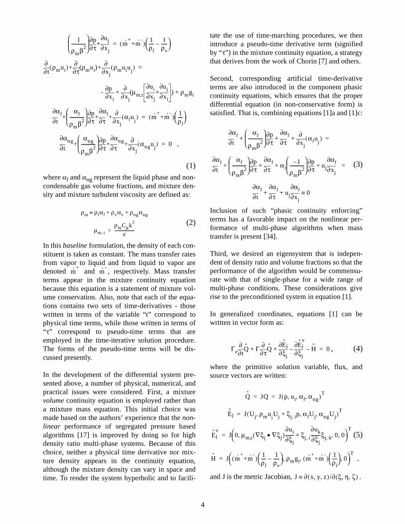
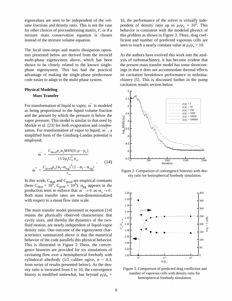
The mass transfer model presented in equation [14]retains the physically observed characteristic thatcavity sizes, and thereby the dynamics of the two-fluid motion, are nearly independent of liquid-vapordensity ratio. One outcome of the eigensystem char-acteristics summarized above is that the numericalbehavior of the code parallels this physical behavior.This is illustrated in Figure 2 There, the conver-gence histories are provided for six simulations ofcavitating flow over a hemispherical forebody withcylindrical afterbody (1/2 caliber ogive, σ = 0.3,from series of results presented below). As the den-sity ratio is increased from 1 to 10, the convergencehistory is modified somewhat, but beyond ρl/ρv =

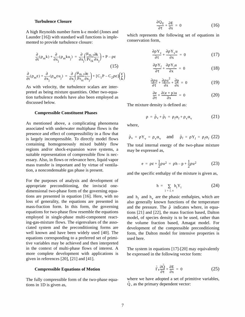
10, the performance of the solver is virtually inde-pendent of density ratio up to ρl/ρv = 105. Thisbehavior is consistent with the modeled physics ofthis problem as shown in Figure 3. There, drag coef-ficient and number of predicted vaporous cells areseen to reach a nearly constant value at ρl/ρv > 10.

As the authors have evolved this work into the anal-ysis of turbomachinery, it has become evident thatthe present mass transfer model has some shortcom-ings in that it does not accommodate thermal effectson cavitation breakdown performance in turboma-chinery [5]. This is discussed further in the pumpcavitation results section below.

m·-

m·+

m·- Cdestρvα

lMIN 0 p pv–,[ ]

1/2ρlU∞2( )t∞

---------------------------------------------------------------=

m·+ Cprodρv αl αng–( )2

1 αl– αng–( )t∞

---------------------------------------------------------------------------------=

m·+

0→ αv 0→

0 500 1000 1500 2000Iteration

-5.5

-5

-4.5

-4

-3.5

-3

-2.5

-2

-1.5

-1

log 10

RM

S[∆

u]

ρl/ρv = 1ρl/ρv = 10ρl/ρv = 100ρl/ρv = 1000ρl/ρv = 10000ρl/ρv = 100000

Figure 2. Comparison of convergence histories with den-sity ratio for hemispherical forebody simulation.

100 101 102

ρl/ρcv

1.00

1.02

1.04

1.06

1.08

1.10

1.12

1.14

1.16

1.18

1.20

CD/C

D, 1φ

0

50

100

150

200

250

300

350

400

# α l <

1 c

ells

Figure 3. Comparison of predicted drag coefficient and number of vaporous cells with density ratio for

hemispherical forebody simulation.

6

Turbulence Closure

A high Reynolds number form k-ε model (Jones andLaunder [16]) with standard wall functions is imple-mented to provide turbulence closure:

(15)

As with velocity, the turbulence scalars are inter-preted as being mixture quantities. Other two-equa-tion turbulence models have also been employed asdiscussed below.

Compressible Constituent Phases

As mentioned above, a complicating phenomenaassociated with underwater multiphase flows is thepresence and effect of compressibility in a flow thatis largely incompressible. To directly model flowscontaining homogeneously mixed bubbly flowregions and/or shock-expansion wave systems, asuitable representation of compressible flow is nec-essary. Also, in flows or relevance here, liquid vapormass transfer is important and by virtue of ventila-tion, a noncondensable gas phase is present.

For the purposes of analysis and development ofappropriate preconditioning, the inviscid one-dimensional two-phase form of the governing equa-tions are presented in equation [16]. Here, with noloss of generality, the equations are presented inmass-fraction form. In this form, the governingequations for two-phase flow resemble the equationsemployed in single-phase multi-component react-ing-gas-mixture flows. The eigenvalues of the asso-ciated system and the preconditioning forms arewell known and have been widely used [40]. Theequations corresponding to a preferred set of primi-tive variables may be achieved and then interpretedin the context of multi-phase flows of interest. Amore complete development with applications isgiven in references [20], [21] and [41].

Compressible Equations of Motion

The fully compressible form of the two-phase equa-tions in 1D is given as,

(16)

which represents the following set of equations inconservation form,

(17)

(18)

(19)

(20)

The mixture density is defined as:

(21)

where,

and (22)

The total internal energy of the two-phase mixturemay be expressed as,

(23)

and the specific enthalpy of the mixture is given as,

(24)

and and are the phasic enthalpies, which arealso generally known functions of the temperatureand the pressure. The indicates where, in equa-tions [21] and [22], the mass fraction based, Daltonmodel, of species density is to be used, rather thanthe volume fraction based, Amagat model. Fordevelopment of the compressible preconditioningform, the Dalton model for intensive properties isused here.

The system in equations [17]-[20] may equivalentlybe expressed in the following vector form:

(25)

where we have adopted a set of primitive variables,, as the primary dependent vector:

t∂∂ ρmk( )

xj∂∂ ρmku

j( )+

xj∂∂ µm t,

Prtk-----------

xj∂∂k

P ρε–+=

t∂∂ ρmε( )

xj∂∂ ρmεu

j( )+

xj∂∂ µm t,

Prtε-----------

xj∂∂ε

C1P C2ρε–[ ]+

εk---

=

∂QY

∂τ-----------

∂E∂x------+ 0=

∂ρYv

∂τ-------------

∂ρYvu

∂x-----------------+ 0=

∂ρYl

∂τ------------

∂ρYlu

∂x----------------+ 0=

∂ρu∂τ

---------∂ρu

2

∂x------------

∂p∂x------+ + 0=

∂e∂τ-----

∂ e p+( )u∂x

-----------------------+ 0=

ρ ρv ρl+ ρlαl ρvαv+= =

ρv ρYv ρvαv= = ρl ρYl ρlαl= =

e ρε 12---ρu2+ ρh p–

12---ρu2+= =

h hiYii l v,=

∑=

hl hv

ρ

Γe∂Q∂τ-------

∂E∂x------+ 0=

Q

7

The corresponding system flux Jacobian is definedas:

(26)

Note that a standard notation has been used to indi-cate partial differentiation with respect to the vari-ables in . The eigenvalues of the above systemare:

(27)

where the speed of sound is given by:.

For the multi-phase system, the above partial deriva-tives need to be obtained in terms of the known vol-ume fraction based properties, i.e., and . Their evaluation is therefore notas straightforward as for single-phase multi-compo-nent mixtures.

The relation for the isothermal sound speed is givenin equation [28].

Q

p

Yv

u

T

= E

ρYvu

ρYlu

ρu2

p+

e p+( )u

=

Γe

Yv∂ρ∂p------

Q

ρ Yv∂ρ

∂Yv----------

Q

+

Yl∂ρ∂p------

Q

ρ– Yl∂ρ

∂Yv----------

Q

+

u∂ρ∂p------

Q

u∂ρ

∂Yv----------

Q

1 ρ∂h∂p------

Q

–

– h0∂ρ∂p------

Q

+ ρ ∂h∂Yv----------

Q

h0∂ρ

∂Yv----------

Q

+

0 Yv∂ρ∂T------

Q

0 Yl∂ρ∂T------

Q

ρ u∂ρ∂T------

Q

ρu ρ ∂h∂T------

Q

h0∂ρ∂T------

Q

+

=

A

uYv∂ρ∂p------

Q

ρu uYv∂ρ

∂Yv----------

Q

+

uYl∂ρ∂p------

Q

ρu– uYl∂ρ

∂Yv----------

Q

+

1 u+ 2∂ρ∂p------

Q

u2 ∂ρ∂Yv----------

Q

ρu∂h∂p------

Q

uh0∂ρ∂p------

Q

+ ρu∂h

∂Yv----------

Q

uh0∂ρ

∂Yv----------

Q

+

ρYv uYv∂ρ∂T------

Q

ρYl uYl∂ρ∂T------

Q

2ρu u2 ∂ρ∂T------

Q

ρ h0 u2+( ) ρu∂h∂T------

Q

uh0∂ρ∂T------

Q

+

=

Q

λ Γe[ ]1–A( ) u u u c±, ,=

c2

ρ ∂h∂T------

Q

ρ∂ρ∂p------

Q

∂h∂T------

Q

∂ρ∂T------

Q

+ 1 ρ∂h∂p------

Q

–

------------------------------------------------------------------------------=

ρv ρv p T,( )=ρl ρl p T,( )=

8

(28)

Preconditioned Compressible Equations of Motion

The preconditioned version of equation [25] may bewritten as:

(29)

where the preconditioning matrix is given by:

(30)

The eigenvalues of the preconditioned system canbe shown to be:

(31)

where the preconditioned pseudo-sound-speed is:

(32)

Definition of Pseudo-Sound Speed

The definition of the pseudo-sound speed is selectedto render the eigenvalues of the preconditioned sys-tem well conditioned. Examining equation [31], wenote that this is readily achieved by choosing:

(33)

where V is local convective velocity magnitude.This form corresponds to the standard inviscidchoice of this parameter. From equation [32], wemay thus express the preconditioning parameter inequation [30]:

(34)

Numerical Method

The baseline numerical method is evolved from theUNCLE code of Taylor and his co-workers at Mis-sissippi State University ([39], for example).UNCLE is based on a single-phase, pseudo-com-pressibility formulation. Roe-based flux differencesplitting is utilized for convection term discretiza-tion. An implicit procedure is adopted with inviscidand viscous flux Jacobians approximated numeri-cally. A block-symmetric Gauss-Seidel iteration isused to solve the approximate Newton system ateach time-step.

The multi-phase extension of the code retains theseunderlying numerics but also incorporates two vol-ume fraction transport equations, mass transfer, non-diagonal preconditioning, flux limiting, dual-time-stepping, and two-equation turbulence modeling.Solution of the fully compressible version requiresenergy conservation.

Discretization

The transformed system of governing equations isdiscretized using a cell centered finite volume pro-cedure. Flux derivatives are computed as

∂ρ∂p------

Q

ραl

ρl-----

∂ρL

∂p---------

Q

αv

ρv------

∂ρv

∂p---------

Q

+=

1

c2

-----

T

∂ρ∂p------

Q

=

Γ∂Q∂τ-------

∂E∂x------+ 0=

Γ

Yv∂ρ′∂p--------

Q

ρ Yv∂ρ

∂Yv----------

Q

+

Yl∂ρ′∂p--------

Q

ρ– Yl∂ρ

∂Yv----------

Q

+

u∂ρ′∂p--------

Q

u∂ρ

∂Yv----------

Q

1 ρ∂h∂p------

Q

–

– h0∂ρ′∂p--------

Q

+ ρ ∂h∂Yv----------

Q

h0∂ρ

∂Yv----------

Q

+

0 Yv∂ρ∂T------

Q

0 Yl∂ρ∂T------

Q

ρ u∂ρ∂T------

Q

ρu ρ ∂h∂T------

Q

h0∂ρ∂T------

Q

+

=

λ Γ1–A( ) u u

12--- u 1

c′c----

2+

u2

1c′c----

2–

24c′2+±, ,=

c′( )2

ρ ∂h∂T------

Q

ρ∂ρ′∂p--------

Q

∂h∂T------

Q

∂ρ∂T------

Q

+ 1 ρ∂h∂p------

Q

–

--------------------------------------------------------------------------------=

c′( )2 Min V2 c2,( )=

∂ρ′∂p--------

Q

1

c′( )2------------

∂ρ∂T------

Q

1 ρ∂h∂p------

Q

–

ρ ∂h∂T------

Q

-------------------------------------------–=

9

, (35)

with similar expressions for , , and thecorresponding viscous fluxes. The inviscid numeri-cal fluxes are evaluated using a flux difference split-ting procedure [45]:

(36)

where, with the non-diagonal preconditioner usedhere, the matrix dissipation operator is defined by

.

The extrapolated Riemann variables, and are obtained using a MUSCL procedure ([2],

for example):

(37)

For first order accuracy, φ = 0. The choice φ = 1, κ =1/3, yields the third order accurate upwind biasscheme used for the results presented in this paper.

The flows of interest here typically contain regionswith sharp interfaces between liquid and gas phases.In addition, compressible flows admit shock wavesand contact discontinuities. Accordingly, higherorder discretization practices are required to retainadequate interface fidelity in the simulations. This isparticularly important in three-dimensional super-cavitating vehicle or control surface computationssuch as those presented below. There, predicted liftand drag can be severely over-predicted if liquidphase (and its much higher inertia) diffuses numeri-cally into low-lift gaseous regions of the lifting sur-face.

Attendant to the third order upwind bias schemeemployed are overshoots in solution variables atthese interfaces. These can be highly destabilizing,particularly for the volume fraction equations, if suf-ficient mass transfer or non-condensable vapor ispresent to yield locally. To ameliorate thisdifficulty, the flux evaluation is rendered locally firstorder in the presence of large gradients in αl or αng.In solutions obtained for incompressible phasic con-

stituents, this is affected through the use of a “dissi-pation sensor” in the spirit of Jameson et al. [14].Specifically, a sensor is formulated for each coordi-nate direction as

. (38)

This parameter is very small except in the immedi-ate vicinity of liquid-gas interfaces. In this work, thehigher order component of the numerical flux inequation [37], i.e. term φ, is multiplied by (1-νi). Incompressible solutions, shocks and contact disconti-nuities are admissible. Hence, it is necessary to limitinterpolations based on the entire primitive vector. Astandard form of the van Albada limiter [13] hasbeen employed.

To illustrate the foregoing discretization issues, con-sider adjacent parallel streams of two constituents.In the absence of shear, if a flow-aligned Cartesianmesh is employed, the mixing layer interface will beperfectly preserved using the present modeling (nomass diffusion). This is true independent of the den-sity ratio of the streams and whether first or higherorder discretization is employed. However, if theinterface encounters a region of significant grid non-orthogonality, the interface will be smeared.

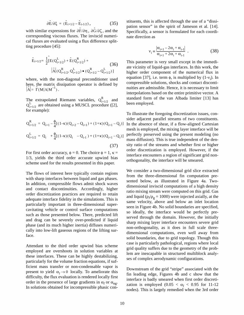
We consider a two-dimensional grid slice extractedfrom the three-dimensional fin computation pre-sented below, as illustrated in Figure 4a. Two-dimensional inviscid computations of a high densityratio mixing stream were computed on this grid. Gasand liquid (ρl/ρg = 1000) were injected axially, at thesame velocity, above and below an inlet locationseen in Figure 4b. No solid boundaries are specified,so ideally, the interface would be perfectly pre-served through the domain. However, the initiallysharp mixing layer interface encounters severe gridnon-orthogonality, as it does in full scale three-dimensional computations, even well away fromsolid boundaries, due to grid topology. Though thiscase is particularly pathological, regions where localgrid quality suffers due to the geometry of the prob-lem are inescapable in structured multiblock analy-ses of complex aerodynamic configurations.

Downstream of the grid “stripe” associated with thefin leading edge, Figures 4b and c show that theinterface is badly smeared when first order discreti-zation is employed (0.05 < αl < 0.95 for 11-12nodes). This is largely remedied when the 3rd order

∂E/∂ξ Ei+1/2 Ei-1/2–( )=

∂F/∂η ∂G/∂ζ

Ei+1/212---[E

ˆQi+1/2

L( ) E Qi+1/2R( )+= +

A Qi+1/2R

Qi+1/2L,( ) Qi+1/2

RQi+1/2

L–( ) ]•

A Γ= M Λ M1–( )

Qi+1/2R

Qi+1/2L

Qi+1/2R

Qi+1φ4--- 1-κ( ) Qi+2 Qi+1–( ) 1+κ( ) Qi+1 Qi–( )+[ ]–=

Qi+1/2L

Qi φ4--- 1-κ( ) Qi Qi-1 –( ) 1+κ( ) Qi+1 Qi–( )+[ ]+=

αl 0→

νi

αi+1 2αi– αi-1+

αi+1 2αi αi-1+ +-------------------------------------------≡

10

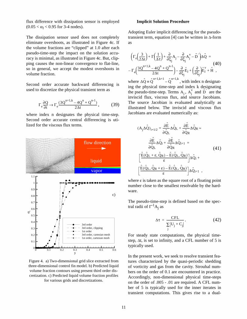
flux difference with dissipation sensor is employed(0.05 < αl < 0.95 for 3-4 nodes).

The dissipation sensor used does not completelyeliminate overshoots, as illustrated in Figure 4c. Ifthe volume fractions are “clipped” at 1.0 after eachpseudo-time-step the impact on the solution accu-racy is minimal, as illustrated in Figure 4c. But, clip-ping causes the non-linear convergence to flat-line,so in general, we accept the modest overshoots involume fraction.

Second order accurate backward differencing isused to discretize the physical transient term as

, (39)

where index n designates the physical time-step.Second order accurate central differencing is uti-lized for the viscous flux terms.

Implicit Solution Procedure

Adopting Euler implicit differencing for the pseudo-transient term, equation [4] can be written in ∆-formas

(40)

where , with index n designat-ing the physical time-step and index k designatingthe pseudo-time-step. Terms , and are theinviscid flux, viscous flux, and source Jacobians.The source Jacobian is evaluated analytically asillustrated below. The inviscid and viscous fluxJacobians are evaluated numerically as:

(41)

where ε is taken as the square root of a floating pointnumber close to the smallest resolvable by the hard-ware.

The pseudo-time-step is defined based on the spec-tral radii of Γ-1Aj as

. (42)

For steady state computations, the physical time-step, ∆t, is set to infinity, and a CFL number of 5 istypically used.

In the present work, we seek to resolve transient fea-tures characterized by the quasi-periodic sheddingof vorticity and gas from the cavity. Strouhal num-bers on the order of 0.1 are encountered in practice.Accordingly, non-dimensional physical time-stepson the order of .005 - .01 are required. A CFL num-ber of 5 is typically used for the inner iterates intransient computations. This gives rise to a dual-

Γe∂Q∂t------- Γe

3Qn+1,k

4Qn

– Qn-1

+( )2∆t

---------------------------------------------------------→

vapor

liquid

flow direction

0 0.1 0.2 0.3 0.4 0.5 0.6y

0

0.1

0.2

0.3

0.4

0.5

0.6

0.7

0.8

0.9

1

1.1

α l

3rd order3rd order, clipping1st order3rd order, cartesian mesh1st order, cartesian mesh

Figure 4. a) Two-dimensional grid slice extracted from three-dimensional control fin model. b) Predicted liquid volume fraction contours using present third order dis-cretization. c) Predicted liquid volume fraction profiles

for various grids and discretizations.

c)

Γe3

2∆t---------

Γ 1∆τ------

∂∂ξj-------Aj

∂∂ξj-------Aj

v– D

-–+ +

∆Q =

Γe3Q

n+1,k4Q

n– Q

n-1+

2∆t----------------------------------------------------

–∂

∂ξj-------Ej–

∂∂ξj-------

Ejv

H ,+ +

∆Q Qn+1,k+1

Qn+1,k

–≡

Aj Ajv

D-

Aj∆Q( )i+1/2∂E

∂QL

----------∆QL=∂E

∂QR

-----------∆QR+ ≈

∂E

∂QL

----------∆Qi∂E

∂QR

-----------∆Qi+1+ =

E QL ε QR,+( ) E QL QR,( )–ε

--------------------------------------------------------------------- ∆Qi +

E QL QR, ε+( ) E QL QR,( )–ε

--------------------------------------------------------------------- ∆Qi+1 ,

∆τ CFL

Uj Cj+j

∑--------------------------=

11

time scheme that provides a 1 to 3 order-of-magni-tude drop in residuals in 5-10 pseudo-time-steps.

Optimum non-linear convergence is obtained usinga pseudo-compressibility parameter, β2/U2

∞ ≅ 10.

Upon application of the discretization and numericallinearization strategies defined, equation [40] repre-sents an algebraic system of equations for ∆Q. Thisblock (6x6 blocks) septadiagonal system is solvediteratively using a block symmetric Gauss-Seidelmethod. Five sweeps of the BSGS scheme areapplied at each pseudo-time-step.

Source Terms

Following the strategy of Venkateswaran et al. [40]for the numerical treatment of mass transfer sourceterms in reacting flow computations, we identify asource and sink component of the mass transfermodel and treat the sink term implicitly and thesource term explicitly. Specifically, with referenceto equation [1] we have

. (43)

With from equation [14] we have

. (44)

It can easily be shown that the non-zero eigenvalueof D- is

(45)

which is less than zero for ρv < ρl. Hence, the identi-fication of as a sink is numerically valid.Implicit treatment of this term provides that αlapproaches zero exponentially, so that cases likethose considered below, where significant masstransfer results in extremely low liquid volume frac-tions, remain stable.

The production mass transfer term is treated explic-itly. A relaxation factor of 0.1 is applied at eachpseudo-time-step to keep this term from destabiliz-ing the code in early iterations.

Turbulence Model Implementation

The turbulence transport equations are solved subse-quent to the mean flow equations at each pseudo-

time-step. A first order accurate flux differencesplitting procedure similar to that outlined above forthe mean flow equations is utilized for convectionterm discretization. The k and ε equations are solvedimplicitly using conventional implicit source termtreatments and a 2x2 block symmetric Gauss-Seidelprocedure.

Boundary Conditions

Velocity components, volume fractions, turbulenceintensity, and length scale are specified at inflowboundaries and extrapolated at outflow boundaries.Pressure distribution is specified at outflow bound-aries (p=0 for single-phase or non-buoyant multi-phase computations) and extrapolated at inflowboundaries. At walls, pressure and volume fractionsare extrapolated, and velocity components and tur-bulence quantities are enforced using conventionalwall functions. Boundary conditions are imposed ina purely explicit fashion by loading “dummy” cellswith appropriate values at each pseudo-time-step.

Parallel Implementation

The multiblock code is instrumented with MPI forparallel execution based on domain decomposition.Inter-block communication is affected at the non-linear level through boundary condition updates andat the linear solver level by loading ∆Q from adja-cent blocks into “dummy” cells at each SGS sweep.This is not as implicit as solving an optimallyordered linear system for the entire domain at eachSGS sweep, but, as demonstrated below, this poten-tial shortcoming will not deteriorate the non-linearperformance of the scheme if the linear solver resid-uals are reduced adequately at each pseudo-time-step. The authors routinely employ 48-80 processorsfor three-dimensional, unsteady analyses.

RESULTS

Three sets of results from the authors’ recentresearch are presented. The first set includes axi-symmetric steady-state and transient analyses of nat-ural and ventilated cavitation about severalconfigurations. These solutions are compared toexperimental measurements to demonstrate thecapability of the modeling employed. The secondset of results includes a variety three-dimensionalanalyses of sheet- and supercavitating flows of rele-vance to high speed vehicles and turbomachinery.The third set of results includes compressible simu-

H+/-

m·+/- 1

ρl----

1ρv-----–

0 0 0 m·+/- 1

ρl----

0,, , , ,T

=

m·-

∆H-

D-∆Q with D

- ∂H-/∂Q≡,≡

λ D-( ) Cdestρv

1ρl----

1ρv-----–

αl1ρl----

p pv–( )+=

m·-

12

lations of a vehicle propulsion plume and a highspeed supercavitating projectile.

Axisymmetric Analyses

Steady State and Transient Natural and Ventilated Cavitation about a Series of Axi-symmetric Forebodies

Due to the authors’ principal research interests insupercavitating vehicles, an emphasis of our CFDdevelopment and validation efforts has been on axi-symmetric bodies. In this regard, we have used datadue to Rouse and McNown [29] as well as that dueto Stinebring et al. [36], [37] for validation pur-poses.

Rouse and McNown [29] carried out a series ofexperiments wherein cavitation induced by convexcurvature aft of various axisymmetric forebodieswith cylindrical afterbodies was investigated. Atlow cavitation numbers, these flows exhibit naturalcavitation initiating near or just aft of the intersec-tion between the forebody, or cavitator, and thecylindrical body. For each configuration, measure-ments were made across a range of cavitation num-bers, including a single phase case (large σ). Surfacestatic pressure measurements were taken along thecavitator and after-body. Photographs were alsotaken from which approximate bubble size andshape were deduced.

Several of the Rouse-McNown configurations wereanalyzed. These included 0-caliber (blunt), 1/4-cali-ber, 1/2-caliber (hemispherical), 1-caliber, and 2-caliber ogives and conical (22.5o cone half-angle)cavitator shapes. The experiments were performedat Reynolds numbers greater than 100,000 based onmaximum cavitator (i.e., after-body) diameter. Avalue of Re = 136000 was used for the simulations.In order to properly assess grid resolution require-ments, a range of grid sizes was used. For the hemi-spherical and conical configurations, grid sizes of65x17, 129x33 and 257x65 were run. Figure 5 dem-onstrates that differences between predicted surfacepressures for the medium and fine meshes are small.The fine meshes were used for all subsequent calcu-lations presented here. For the blunt fore-body, atwo-block grid topology had to be used, and a meshconsistent with the resolution and clustering of theother head-forms was utilized (65x49, 257x65 forblocks 1 and 2; see Figure 9b).

Figures 6 through 14 show sample results for theseaxisymmetric computations. Figure 6a shows pre-dicted and measured surface pressure distributionsat several cavitation numbers for the 1-caliber ogiveforebody with cylindrical afterbody. As the cavita-tion number is decreased from near a critical “incep-tion” value, a cavitation bubble forms and grows.The presence of the bubble manifests itself as adecrease in magnitude, flattening and lengthening ofthe pressure minimum along the surface. Also, bub-ble closure gives rise to an overshoot in pressurerecovery due to the local stagnation associated withfree-stream liquid flowing over the convex curva-ture at the aft end of the bubble. The code is seen toaccurately capture these physics as evidenced by theclose correspondence between predicted and mea-sured pressure distributions. Figure 6b illustrates thequalitative physics as captured by the model. There,surface pressure contours, field liquid volume frac-tion contours, selected streamlines and the grid usedare shown for the 1-caliber case at σ = 0.15. For thiscase, the cavitation bubble is quite long (L/d > 3).As with all large cavitation bubbles, the closureregion is characterized by an unsteady “re-entrant”jet. The significant flow recirculation and associatedshedding of vorticity and vapor in these flowsrequire that a transient simulation be carried out.This is discussed further below. The solutiondepicted in Figure 6b represents a snapshot in time.

0 1 2 3 4 5s/d

-0.4

-0.2

0

0.2

0.4

0.6

0.8

CP

Fine GridMedium GridCoarse Grid

Figure 5. Comparison of predicted surface pressure distri-butions for naturally cavitating axisymmetric flow over a conical cavitator-cylindrical after-body configuration, σ = 0.3. Coarse (65x17), medium (129x33) and fine (257x65)

mesh solutions are plotted.

13

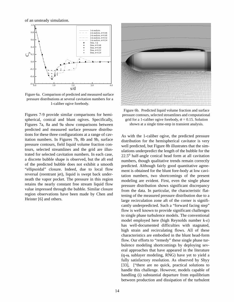
of an unsteady simulation.

Figures 7-9 provide similar comparisons for hemi-spherical, conical and blunt ogives. Specifically,Figures 7a, 8a and 9a show comparisons betweenpredicted and measured surface pressure distribu-tions for these three configurations at a range of cav-itation numbers. In Figures 7b, 8b and 9b, surfacepressure contours, field liquid volume fraction con-tours, selected streamlines and the grid are illus-trated for selected cavitation numbers. In each case,a discrete bubble shape is observed, but the aft endof the predicted bubble does not exhibit a smooth“ellipsoidal” closure. Indeed, due to local flowreversal (reentrant jet), liquid is swept back under-neath the vapor pocket. The pressure in this regionretains the nearly constant free stream liquid flowvalue impressed through the bubble. Similar closureregion observations have been made by Chen andHeister [6] and others.

As with the 1-caliber ogive, the predicted pressuredistribution for the hemispherical cavitator is verywell predicted, but Figure 8b illustrates that the sim-ulations underpredict the length of the bubble for the22.5o half-angle conical head form at all cavitationnumbers, though qualitative trends remain correctlypredicted. Although fairly good quantitative agree-ment is obtained for the blunt fore-body at low cavi-tation numbers, two shortcomings of the presentmodeling are evident. First, even the single phasepressure distribution shows significant discrepancyfrom the data. In particular, the characteristic flat-tening of the measured pressure distribution due to alarge recirculation zone aft of the corner is signifi-cantly underpredicted. Such a “forward facing step”flow is well known to provide significant challengesto single phase turbulence models. The conventionalmodel employed here (high Reynolds number k-ε)has well-documented difficulties with stagnated,high strain and recirculating flows. All of thesecharacteristics are embodied in the blunt head-formflow. Our efforts to “remedy” these single phase tur-bulence modeling shortcomings by deploying sev-eral approaches that have appeared in the literature(q-ω, sublayer modeling, RNG) have yet to yield afully satisfactory resolution. As observed by Shyy[33], [“there are no quick, practical solutions tohandle this challenge. However, models capable ofhandling (i) substantial departure from equilibriumbetween production and dissipation of the turbulent

s/d

Cp

0.0 1.0 2.0 3.0 4.0-0.6

-0.4

-0.2

0.0

0.2

0.4

0.6

0.8

1.0

1-φ analysis2-φ analysis, σ=0.462-φ analysis, σ=0.402-φ analysis, σ=0.322-φ analysis, σ=0.24Data, 1-φData, σ=0.46Data, σ=0.40Data, σ=0.32Data, σ=0.24

Figure 6a. Comparison of predicted and measured surface pressure distributions at several cavitation numbers for a

1-caliber ogive forebody.

Figure 6b. Predicted liquid volume fraction and surface pressure contours, selected streamlines and computational

grid for a 1-caliber ogive forebody, σ = 0.15. Solution shown at a single time-step in transient analysis.

14

kinetic energy, (ii) anisotropy between main Rey-nolds stress components, and (iii) turbulence-enhanced mass transfer across the phase inter-face,should be emphasized”.]

The second modeling shortcoming evident in theblunt head-form results is associated with the slightunderprediction of cavity pressure at intermediatecavitation numbers. Indeed, the analysis predicts alarge cavity at nearly constant pressure (vapor pres-sure) which initiates very close to the leading edge.The data exhibits a higher surface pressure near theleading edge, which approaches the vapor pressurewith increased distance from the leading edge. Thisphenomenon arises due to the presence of a pressureminimum away from the body at the core of thestrong vorticity associated with the leading edgeseparation. Physically, this is where cavitation ini-tiates in this flow. The growth, interaction and trans-port of the small cavitation nuclei then give rise to alarger cavitation bubble emanating from this off-body location. The current modeling is unable tocapture these relevant physics, though local pressureminimums are predicted to occur off-body aft of theleading edge. Attempts to adjust the time constant inequation [14] ( ) have proved unsuccessful,so this also remains an ongoing modeling challenge.

Several parameters of relevance in the characteriza-tion of cavitation bubbles include body diameter, d,bubble length, L, bubble diameter, dm, and formdrag coefficient associated with the cavitator, CD.Some ambiguity is inherent in both the experimentaland computational definition of the latter three ofthese parameters. Bubble closure location is difficultto define due to unsteadiness and its dependence onafter-body diameter (which can range from 0 [iso-lated cavitator] to the cavitator diameter). Accord-ingly, bubble length is often, and here, taken astwice the distance from cavity leading edge to thelocation of maximum bubble diameter (see Figure10). The form drag coefficient is taken as the pres-sure drag on an isolated cavitator shape. For cavita-tors with afterbodies, such as here, the pressurecontribution to CD associated with the back of the

cavitator is assumed equal to the cavity pressure (≅pv). For the simulations, dm is determined by exam-ining the αl = 0.5 contour and determining its maxi-mum radial location.

Cdest/t∞

Figure 7a. Comparison of predicted and measured surface pressure distributions at several cavitation numbers for a

hemispherical fore-body.

0.0 1.0 2.0 3.0 4.0 5.0s/d

-0.8

-0.6

-0.4

-0.2

0

0.2

0.4

0.6

0.8

1

1.2

1.4

CP

1-φ analysis2-φ analysis, σ=0.52-φ analysis, σ=0.42-φ analysis, σ=0.32-φ analysis, σ=0.2Data, 1-φData, σ=0.5Data, σ=0.4Data, σ=0.3Data, σ=0.2

Figure 7b. Predicted liquid volume fraction and surface ressure contours, selected streamlines and computational

grid for a hemispherical fore-body, σ=0.3.

15

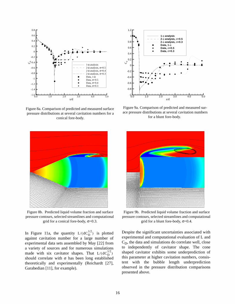
In Figure 11a, the quantity is plottedagainst cavitation number for a large number ofexperimental data sets assembled by May [22] froma variety of sources and for numerous simulationsmade with six cavitator shapes. That should correlate with σ has been long establishedtheoretically and experimentally (Reichardt [27],Garabedian [11], for example).

Despite the significant uncertainties associated withexperimental and computational evaluation of L andCD, the data and simulations do correlate well, closeto independently of cavitator shape. The coneshaped cavitator exhibits some underprediction ofthis parameter at higher cavitation numbers, consis-tent with the bubble length underpredictionobserved in the pressure distribution comparisonspresented above.

Figure 8a. Comparison of predicted and measured surface pressure distributions at several cavitation numbers for a

conical fore-body.

0.0 1.0 2.0 3.0 4.0 5.0s/d

-1.6

-1.4

-1.2

-1

-0.8

-0.6

-0.4

-0.2

0

0.2

0.4

0.6

0.8C

P

1-φ analysis2-φ analysis, σ=0.52-φ analysis, σ=0.42-φ analysis, σ=0.3Data, 1-φData, σ=0.5Data, σ=0.4Data, σ=0.3

Figure 8b. Predicted liquid volume fraction and surface pressure contours, selected streamlines and computational

grid for a conical fore-body, σ=0.3.

L/ dCD1/2( )

L/ dCD1/2( )

0.0 1.0 2.0 3.0 4.0 5.0s/d

-1

-0.8

-0.6

-0.4

-0.2

0

0.2

0.4

0.6

0.8

1

1.2

CP

1-φ analysis2-φ analysis, σ=0.52-φ analysis, σ=0.3Data, 1-φData, σ=0.5Data, σ=0.3

Figure 9a. Comparison of predicted and measured sur-ace pressure distributions at several cavitation numbers

for a blunt fore-body.

Figure 9b. Predicted liquid volume fraction and surface pressure contours, selected streamlines and computational

grid for a blunt fore-body, σ=0.4.

16

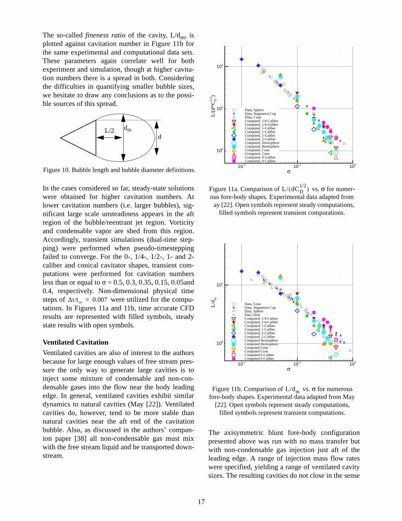
The so-called fineness ratio of the cavity, L/dm, isplotted against cavitation number in Figure 11b forthe same experimental and computational data sets.These parameters again correlate well for bothexperiment and simulation, though at higher cavita-tion numbers there is a spread in both. Consideringthe difficulties in quantifying smaller bubble sizes,we hesitate to draw any conclusions as to the possi-ble sources of this spread.

In the cases considered so far, steady-state solutionswere obtained for higher cavitation numbers. Atlower cavitation numbers (i.e. larger bubbles), sig-nificant large scale unsteadiness appears in the aftregion of the bubble/reentrant jet region. Vorticityand condensable vapor are shed from this region.Accordingly, transient simulations (dual-time step-ping) were performed when pseudo-timesteppingfailed to converge. For the 0-, 1/4-, 1/2-, 1- and 2-caliber and conical cavitator shapes, transient com-putations were performed for cavitation numbersless than or equal to σ = 0.5, 0.3, 0.35, 0.15, 0.05and0.4, respectively. Non-dimensional physical timesteps of were utilized for the compu-tations. In Figures 11a and 11b, time accurate CFDresults are represented with filled symbols, steadystate results with open symbols.

Ventilated Cavitation

Ventilated cavities are also of interest to the authorsbecause for large enough values of free stream pres-sure the only way to generate large cavities is toinject some mixture of condensable and non-con-densable gases into the flow near the body leadingedge. In general, ventilated cavities exhibit similardynamics to natural cavities (May [22]). Ventilatedcavities do, however, tend to be more stable thannatural cavities near the aft end of the cavitationbubble. Also, as discussed in the authors’ compan-ion paper [38] all non-condensable gas must mixwith the free stream liquid and be transported down-stream.

The axisymmetric blunt fore-body configurationpresented above was run with no mass transfer butwith non-condensable gas injection just aft of theleading edge. A range of injection mass flow rateswere specified, yielding a range of ventilated cavitysizes. The resulting cavities do not close in the sense

Figure 10. Bubble length and bubble diameter definitions.

dmL/2d

∆t/t∞ 0.007=

XXX

XXX

XXX

XX

X

σ

L/(

d*C

D1/2 )

10-2 10-1 100

100

101

102

Data, SphereData, Stagnation CupData, ConeComputed, 1/4-CaliberComputed, 1/4-CaliberComputed, 1-CaliberComputed, 1-CaliberComputed, 2-CaliberComputed, 2-CaliberComputed, HemisphereComputed, HemisphereComputed, ConeComputed, ConeComputed, 0-CaliberComputed, 0-Caliber

X

Figure 11a. Comparison of vs. σ for numer-ous fore-body shapes. Experimental data adapted from

ay [22]. Open symbols represent steady computations, filled symbols represent transient computations.

L/ dCD1/2( )

XX

XXX

XXX

XX

XXX

X

X

XX

σ

L/d

m

10-2 10-1 100

100

101

Data, ConeData, Stagnation CupData, SphereData, DiskComputed, 1/4-CaliberComputed, 1/4-CaliberComputed, 1-CaliberComputed, 1-CaliberComputed, 2-CaliberComputed, 2-CaliberComputed HemisphereComputed HemisphereComputed ConeComputed ConeComputed 0-CaliberComputed 0-Caliber

X

Figure 11b. Comparison of vs. σ for numerous fore-body shapes. Experimental data adapted from May

[22]. Open symbols represent steady computations, filled symbols represent transient computations.

L/dm

17

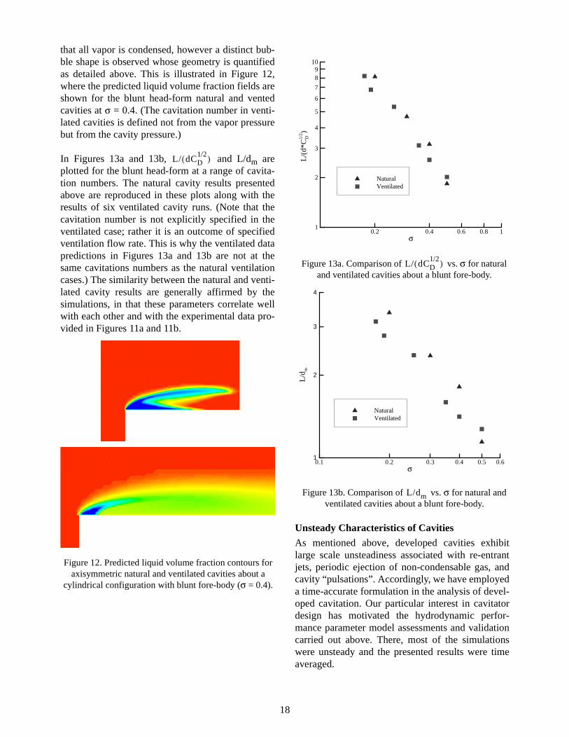
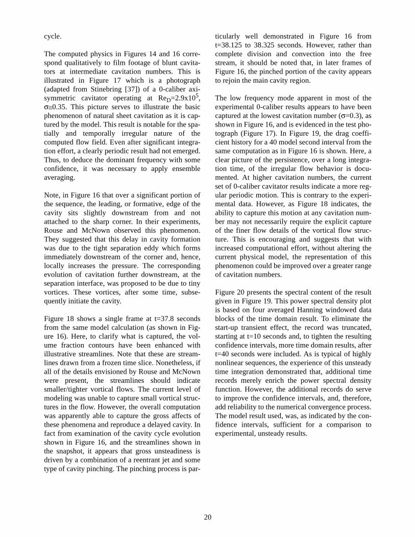
that all vapor is condensed, however a distinct bub-ble shape is observed whose geometry is quantifiedas detailed above. This is illustrated in Figure 12,where the predicted liquid volume fraction fields areshown for the blunt head-form natural and ventedcavities at σ = 0.4. (The cavitation number in venti-lated cavities is defined not from the vapor pressurebut from the cavity pressure.)

In Figures 13a and 13b, and L/dm areplotted for the blunt head-form at a range of cavita-tion numbers. The natural cavity results presentedabove are reproduced in these plots along with theresults of six ventilated cavity runs. (Note that thecavitation number is not explicitly specified in theventilated case; rather it is an outcome of specifiedventilation flow rate. This is why the ventilated datapredictions in Figures 13a and 13b are not at thesame cavitations numbers as the natural ventilationcases.) The similarity between the natural and venti-lated cavity results are generally affirmed by thesimulations, in that these parameters correlate wellwith each other and with the experimental data pro-vided in Figures 11a and 11b.

Unsteady Characteristics of Cavities

As mentioned above, developed cavities exhibitlarge scale unsteadiness associated with re-entrantjets, periodic ejection of non-condensable gas, andcavity “pulsations”. Accordingly, we have employeda time-accurate formulation in the analysis of devel-oped cavitation. Our particular interest in cavitatordesign has motivated the hydrodynamic perfor-mance parameter model assessments and validationcarried out above. There, most of the simulationswere unsteady and the presented results were timeaveraged.

L/ dCD1/2( )

Figure 12. Predicted liquid volume fraction contours for axisymmetric natural and ventilated cavities about a

cylindrical configuration with blunt fore-body (σ = 0.4).

σ

L/(

d*C

D1/2 )

0.2 0.4 0.6 0.8 11

2

3

4

5

6

7

89

10

NaturalVentilated

Figure 13a. Comparison of vs. σ for natural and ventilated cavities about a blunt fore-body.

L/ dCD1/2( )

σ

L/d

m

0.1 0.2 0.3 0.4 0.5 0.61

2

3

4

NaturalVentilated

Figure 13b. Comparison of vs. σ for natural and ventilated cavities about a blunt fore-body.

L/dm

18

There is also particular interest in the time depen-dent (as opposed to time averaged) characteristics ofdeveloped cavities, as these physics play impor-tantly in vehicle acoustics, body wetting and bubblecloud collapse. Motivated by the former two, wehave carried out an assessment of the accuracy ofthe predicted temporal statistics provided by thecode.

We first illustrate the qualitative temporal character-istics of an analysis of a bluff forebody shape atmoderate cavitation numbers. In such flows it iswell known that the entire cavity can be highlyunsteady, with “re-entrant” liquid issuing quasi-peri-odically from the aft end of the bubble and travelingall the way to the front of the bubble. In Figure 14, atime-sequence of predicted vapor volume fraction isreproduced for a 1/4-caliber ogive simulation at aReynolds number of 1.36 x 105 and a cavitationnumber of 0.3. A 193 x 65 mesh and a non-dimen-sional physical time-step of 0.007 was used for thiscomputation. Clearly captured is the transport of aregion of liquid towards the front of the cavity.There, the liquid interacts with the bubble leadingedge, the top of this liquid region being sheared aft-ward while the bulk of the fluid proceeds upstream“pinching off” the bubble near the leading edge.

Figure 15 shows two other elements of this particu-lar transient simulation. The inner- or pseudo-timeconvergence history for four successive physical

time steps is shown in Figure 15a. Nearly a threeorder-of-magnitude drop in the axial velocity residu-als is obtained at each physical time step using 10pseudo-time-steps. Figure 15b shows a segment ofthe time history of predicted drag coefficient for thiscase.

Stinebring et al. [36] documented the unsteadycycling behavior of several axisymmetric cavitators.Their report included results for both ventilated andnatural cavitation. The unsteady performance of 45o

(22.5o half-angle) conical, hemispherical, and 0-cal-iber ogival cavitators at a range of cavitation num-bers were documented. Natural cavitation analysiscomparisons have been included here.

Figure 16 contains a series of snapshots of the pre-dicted volume fraction field from an unsteady modelcomputation of flow over a 0-caliber (blunt) cavita-tor. Here the Reynolds number (based on diameter)was 1.46x105 and the cavitation number was 0.3.This result is presented over an approximate modelcycle. The figure also includes the correspondingtime segment of drag coefficient. Note that thespikes in drag near t=37.725 and t=38.925 secondscorrespond to reductions in the relative amount ofvapor near the sharp leading edge. This marks theprogress of a bulk volume of liquid from the closureregion to the forward end of the cavity as part of thereentrant jet process. Although far from regular,these spikes also delineate the approximate model

Figure 14. Time sequence of predicted vapor volume fraction for flow over a 1/4 caliber ogive with cylindri-

cal afterbody, σ = 0.3

t=0.05

t=0.10

t=0.15

t=0.20

t=0.25

t=0.30

t=0.35

t=0.40

t=0.45

t=0.50

0 10 20 30 40Pseudo-time-step

-5.0

-4.5

-4.0

-3.5

-3.0

-2.5

-2.0

-1.5

log 10

RM

S[∆

u]0.00 0.10 0.20 0.30 0.40 0.50 0.60 0.70

Physical Timestep

0.590

0.595

0.600

0.605

0.610

0.615

0.620

CD

Figure 15. a) Pseudo-time convergence history at four successive physical time steps for transient flow over a

1/4 caliber ogive with cylindrical afterbody, σ = 0.3. b) Segment of time history of predicted CD for this case.

a)

b)

19

cycle.

The computed physics in Figures 14 and 16 corre-spond qualitatively to film footage of blunt cavita-tors at intermediate cavitation numbers. This isillustrated in Figure 17 which is a photograph(adapted from Stinebring [37]) of a 0-caliber axi-symmetric cavitator operating at ReD=2.9x105,σ≅0.35. This picture serves to illustrate the basicphenomenon of natural sheet cavitation as it is cap-tured by the model. This result is notable for the spa-tially and temporally irregular nature of thecomputed flow field. Even after significant integra-tion effort, a clearly periodic result had not emerged.Thus, to deduce the dominant frequency with someconfidence, it was necessary to apply ensembleaveraging.

Note, in Figure 16 that over a significant portion ofthe sequence, the leading, or formative, edge of thecavity sits slightly downstream from and notattached to the sharp corner. In their experiments,Rouse and McNown observed this phenomenon.They suggested that this delay in cavity formationwas due to the tight separation eddy which formsimmediately downstream of the corner and, hence,locally increases the pressure. The correspondingevolution of cavitation further downstream, at theseparation interface, was proposed to be due to tinyvortices. These vortices, after some time, subse-quently initiate the cavity.

Figure 18 shows a single frame at t=37.8 secondsfrom the same model calculation (as shown in Fig-ure 16). Here, to clarify what is captured, the vol-ume fraction contours have been enhanced withillustrative streamlines. Note that these are stream-lines drawn from a frozen time slice. Nonetheless, ifall of the details envisioned by Rouse and McNownwere present, the streamlines should indicatesmaller/tighter vortical flows. The current level ofmodeling was unable to capture small vortical struc-tures in the flow. However, the overall computationwas apparently able to capture the gross affects ofthese phenomena and reproduce a delayed cavity. Infact from examination of the cavity cycle evolutionshown in Figure 16, and the streamlines shown inthe snapshot, it appears that gross unsteadiness isdriven by a combination of a reentrant jet and sometype of cavity pinching. The pinching process is par-

ticularly well demonstrated in Figure 16 fromt=38.125 to 38.325 seconds. However, rather thancomplete division and convection into the freestream, it should be noted that, in later frames ofFigure 16, the pinched portion of the cavity appearsto rejoin the main cavity region.

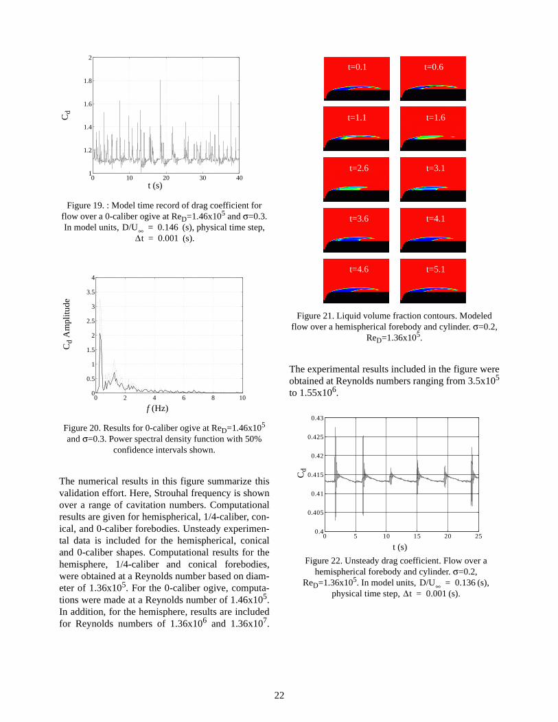
The low frequency mode apparent in most of theexperimental 0-caliber results appears to have beencaptured at the lowest cavitation number (σ=0.3), asshown in Figure 16, and is evidenced in the test pho-tograph (Figure 17). In Figure 19, the drag coeffi-cient history for a 40 model second interval from thesame computation as in Figure 16 is shown. Here, aclear picture of the persistence, over a long integra-tion time, of the irregular flow behavior is docu-mented. At higher cavitation numbers, the currentset of 0-caliber cavitator results indicate a more reg-ular periodic motion. This is contrary to the experi-mental data. However, as Figure 18 indicates, theability to capture this motion at any cavitation num-ber may not necessarily require the explicit captureof the finer flow details of the vortical flow struc-ture. This is encouraging and suggests that withincreased computational effort, without altering thecurrent physical model, the representation of thisphenomenon could be improved over a greater rangeof cavitation numbers.

Figure 20 presents the spectral content of the resultgiven in Figure 19. This power spectral density plotis based on four averaged Hanning windowed datablocks of the time domain result. To eliminate thestart-up transient effect, the record was truncated,starting at t=10 seconds and, to tighten the resultingconfidence intervals, more time domain results, aftert=40 seconds were included. As is typical of highlynonlinear sequences, the experience of this unsteadytime integration demonstrated that, additional timerecords merely enrich the power spectral densityfunction. However, the additional records do serveto improve the confidence intervals, and, therefore,add reliability to the numerical convergence process.The model result used, was, as indicated by the con-fidence intervals, sufficient for a comparison toexperimental, unsteady results.

20

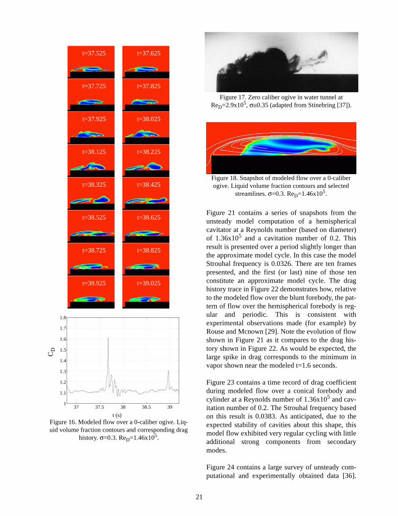
Figure 21 contains a series of snapshots from theunsteady model computation of a hemisphericalcavitator at a Reynolds number (based on diameter)of 1.36x105 and a cavitation number of 0.2. Thisresult is presented over a period slightly longer thanthe approximate model cycle. In this case the modelStrouhal frequency is 0.0326. There are ten framespresented, and the first (or last) nine of those tenconstitute an approximate model cycle. The draghistory trace in Figure 22 demonstrates how, relativeto the modeled flow over the blunt forebody, the pat-tern of flow over the hemispherical forebody is reg-ular and periodic. This is consistent withexperimental observations made (for example) byRouse and Mcnown [29]. Note the evolution of flowshown in Figure 21 as it compares to the drag his-tory shown in Figure 22. As would be expected, thelarge spike in drag corresponds to the minimum invapor shown near the modeled t=1.6 seconds.

Figure 23 contains a time record of drag coefficientduring modeled flow over a conical forebody andcylinder at a Reynolds number of 1.36x105 and cav-itation number of 0.2. The Strouhal frequency basedon this result is 0.0383. As anticipated, due to theexpected stability of cavities about this shape, thismodel flow exhibited very regular cycling with littleadditional strong components from secondarymodes.

Figure 24 contains a large survey of unsteady com-putational and experimentally obtained data [36].

t=37.525 t=37.625

t=37.725 t=37.825

t=37.925 t=38.025

t=38.125 t=38.225

t=38.325 t=38.425

t=38.525 t=38.625

t=38.725 t=38.825

t=38.925 t=39.025

37 37.5 38 38.5 391

1.1

1.2

1.3

1.4

1.5

1.6

1.7

1.8

Figure 16. Modeled flow over a 0-caliber ogive. Liq-uid volume fraction contours and corresponding drag

history. σ=0.3. ReD=1.46x105.

CD

t (s)

Figure 17. Zero caliber ogive in water tunnel at ReD=2.9x105, σ≅0.35 (adapted from Stinebring [37]).

Figure 18. Snapshot of modeled flow over a 0-caliber ogive. Liquid volume fraction contours and selected

streamlines. σ=0.3. ReD=1.46x105.

21

The numerical results in this figure summarize thisvalidation effort. Here, Strouhal frequency is shownover a range of cavitation numbers. Computationalresults are given for hemispherical, 1/4-caliber, con-ical, and 0-caliber forebodies. Unsteady experimen-tal data is included for the hemispherical, conicaland 0-caliber shapes. Computational results for thehemisphere, 1/4-caliber and conical forebodies,were obtained at a Reynolds number based on diam-eter of 1.36x105. For the 0-caliber ogive, computa-tions were made at a Reynolds number of 1.46x105.In addition, for the hemisphere, results are includedfor Reynolds numbers of 1.36x106 and 1.36x107.

The experimental results included in the figure wereobtained at Reynolds numbers ranging from 3.5x105

to 1.55x106.

Figure 19. : Model time record of drag coefficient for flow over a 0-caliber ogive at ReD=1.46x105 and σ=0.3. In model units, (s), physical time step,

(s).

Figure 20. Results for 0-caliber ogive at ReD=1.46x105 and σ=0.3. Power spectral density function with 50%

confidence intervals shown.

0 10 20 30 401

1.2

1.4

1.6

1.8

2C

d

t (s)

D/U∞ 0.146=∆t 0.001=

0 2 4 6 8 100

0.5

1

1.5

2

2.5

3

3.5

4

f (Hz)

Cd

Am

plitu

de

Figure 21. Liquid volume fraction contours. Modeled flow over a hemispherical forebody and cylinder. σ=0.2,

ReD=1.36x105.

t=0.1 t=0.6

t=1.1 t=1.6

t=2.6 t=3.1

t=3.6 t=4.1

t=4.6 t=5.1

0 5 10 15 20 250.4

0.405

0.41

0.415

0.42

0.425

0.43

Figure 22. Unsteady drag coefficient. Flow over a hemispherical forebody and cylinder. σ=0.2,

ReD=1.36x105. In model units, (s), physical time step, (s).

D/U∞ 0.136=∆t 0.001=

Cd

t (s)

22

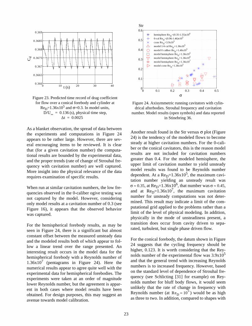
As a blanket observation, the spread of data betweenthe experiments and computations in Figure 24appears to be rather large. However, there are sev-eral encouraging items to be reviewed. It is clearthat (for a given cavitation number) the computa-tional results are bounded by the experimental data,and the proper trends (rate of change of Strouhal fre-quency with cavitation number) are well captured.More insight into the physical relevance of the datarequires examination of specific results.

When run at similar cavitation numbers, the low fre-quencies observed in the 0-caliber ogive testing wasnot captured by the model. However, consideringonly model results at a cavitation number of 0.3 (seeFigure 16), it appears that the observed behaviorwas captured.

For the hemispherical forebody results, as may beseen in Figure 24, there is a significant but almostconstant offset between the measured unsteady dataand the modeled results both of which appear to fol-low a linear trend over the range presented. Aninteresting result occurs in the model data for thehemispherical forebody with a Reynolds number of1.36x107 (pentagrams in Figure 24). Here thenumerical results appear to agree quite well with theexperimental data for hemispherical forebodies. Theexperiments were taken at an order of magnitudelower Reynolds number, but the agreement is appar-ent in both cases where model results have beenobtained. For design purposes, this may suggest anavenue towards model calibration.

Another result found in the Str versus σ plot (Figure24) is the tendency of the modeled flows to becomesteady at higher cavitation numbers. For the 0-cali-ber or the conical cavitators, this is the reason modelresults are not included for cavitation numbersgreater than 0.4. For the modeled hemisphere, theupper limit of cavitation number to yield unsteadymodel results was found to be Reynolds numberdependent. At a ReD=1.36x105, the maximum cavi-tation number yielding an unsteady result was

, at ReD=1.36x106, that number was ,and at ReD=1.36x107, the maximum cavitationnumber for unsteady computations was not deter-mined. This result may indicate a limit of the com-putational grid applied to the problems rather than alimit of the level of physical modeling. In addition,physically in the mode of unsteadiness present, atransition does occur from cavity driven to sepa-rated, turbulent, but single phase driven flow.

For the conical forebody, the datum shown in Figure24 suggests that the cycling frequency should behigher, 0.123. It is worth considering that the Rey-nolds number of the experimental flow was 3.9x105

and that the general trend with increasing Reynoldsnumbers is to increased frequency. However, basedon the standard level of dependence of Strouhal fre-quency (see Schlicting [31] for example) on Rey-nolds number for bluff body flows, it would seemunlikely that the rate of change in frequency withReynolds number (at ) would be as highas three to two. In addition, compared to shapes with

Figure 23. Predicted time record of drag coefficient for flow over a conical forebody and cylinder at

ReD=1.36x105 and σ=0.3. In model units, (s), physical time step, D/U∞ 0.136=

∆t 0.0025=

0 10 20 30 400.366

0.3665

0.367

0.3675

0.368

0.3685

0.369C

d

t (s)

Figure 24. Axisymmetric running cavitators with cylin-drical afterbodies. Strouhal frequency and cavitation

number. Model results (open symbols) and data reported in Stinebring 36.

0 0.1 0.2 0.3 0.4 0.50

0.1

0.2

0.3

0.4

0.5

0.6hemisphere ReD=(0.35-1.55)x106

0-cal ReD=(0.96-1.46)x105

cone ReD=3.9x105

model 1/4 cal ReD=1.36x105

model 0 caliber ReD=1.46x105

model hemisphere ReD=1.36x105

model hemisphere ReD=1.36x106

model hemisphere ReD=1.36x107

model cone ReD=1.36x105

σ

Str

σ 0.35≈ σ 0.45≈

ReD 105≈

23

geometrically smooth surfaces, the nature ofunsteady flow over a conical shape is not expectedto be nearly so dependent on Reynolds number. Inthe case of a cone, at low values of cavitation num-ber (i.e. σ=0.3), the separation location, and, hence,the likely forward location of the cavity, is rarely inquestion.

A trend that is captured in the model results but notrepresented in the experimental data included here,is the tendency for the Strouhal frequency of a givencavitator shape to exhibit two distinct flow regimes.The first regime exists at moderate cavitation num-bers and is indicated by a low Strouhal frequencywhere the value of Str will have an apparent lineardependence on σ. The second regime tends towardmuch higher cycling frequencies. Here the depen-dent Strouhal frequency appears to asymptoticallyapproach a vertical line with higher cavitation num-ber, just prior to the complete elimination of the cav-ity. This is documented in Stinebring [36] anddemonstrated in Figure 24 for the modeled hemi-sphere at ReD=1.36x106. Based on the modelresults, it appears that this is characteristic of achange from a flow mode dominated by a largeunsteady cavity to one dominated by other, single-phase, turbulent, sources of unsteadiness.

During this investigation, some effort towards theestablishment of temporal and spatial discretizationindependence was made. As a requirement of themodel, to accommodate the use of wall functions,for regions of attached liquid flow, fine-grid near-wall points were established at locations yielding10<y+<100.

Temporal convergence was established by the suc-cessive reduction of time integration step for aselected few cases. Figure 25 contains a comparisonof the spectral content of results for flow over ahemispherical forebody and cylindrical afterbody,with ReD=1.36x105 and σ=0.3, for three, succes-sively smaller, integration step sizes. Here, with aphysical time step, seconds, the compu-tation resulted in a Strouhal frequency, Str=0.0680,with a time step, seconds, Str=0.0622,and with seconds, Str=0.0680. Moresignificantly, as demonstrated in the figure, for thesmaller two integration step sizes, over the range ofrelevant (shown) frequencies, there was very similarmodal behavior.

Unfortunately only the fine-grid models tended to

provide unsteady results. Thus time and spatialfidelity were judged independently. A demonstra-tion of the steady-state spatial convergence of themodeled conical forebody and cylindrical afterbodyis given in Figure 5.

Three-Dimensional Analyses

Natural Cavitation about 1/2- and 1-Caliber Ogives

In order to demonstrate the three-dimensional capa-bility of the method, a model of the hemisphericalfore-body configuration studied above was run atnumerous angles of attack and a cavitation numberof 0.3. A 97x33x65 mesh was utilized (correspond-ing to the “medium” mesh size discussed in gridstudies above). The domain was decomposed into 8subdomains azimuthally and run on 8 SGI RS10KOctane machines. Parallel efficiencies of 85% wereachieved for these problems.

Figure 26 provides sample results for angles ofattack of 0.0o, 2.5o, 5.0o and 7.5o. These plotsinclude pressure contours on the plane of symmetry,sample streamlines and the cavitation bubble shapeas identified with an isosurface of αl = 0.99. Severalinteresting features are observed in the predictions.In particular, the flows are seen to be highly three-dimensional in nature at angle-of-attack. A recircu-lation zone aft of the bubble, grows with angle ofattack. This diminishes the local pressure recoveryassociated with the bubble-induced blockage andthis in turn leads to a local collapse of the bubble on

∆t 0.005=

∆t 0.0025=∆t 0.001=

Figure 25. Spectral comparison of effect of physical inte-gration time step size on Cd history. Model result. Flow

over a hemispherical forebody with cylindrical afterbody. ReD=1.36x105. σ=0.3.

0 2 4 6 8 1010

−8

10−6

10−4

10−2

∆t=0.005∆t=0.0025∆t=0.001

f

Cd

Am

plit

ude

24

the top of the body. Indeed at angle-of-attack thebubble is seen to have its greatest axial extent off ofthe symmetry plane of the geometry.

Figure 27 shows the results of a three-dimensionalsimulation of cavitating flow over a 1-caliber ogiveforebody with cylindrical afterbody at a 10o angle-of-attack. A cavitation number of 0.32 was speci-fied. Again a 97 x 33 x 65 mesh was utilized, thedomain was decomposed into eight subdomains azi-muthally and run on eight processors and at this cav-itation number using this grid a steady state solutioncould be obtained. Figure 27 illustrates the predictedbubble shape and streamline pattern for this simula-tion. The bubble shape is highly three-dimensionalin nature; it does not close on the pressure side ofthe body. The streamline pattern is characterized bya large recirculation zone aft of the bubble and sig-nificant azimuthally oriented vortical structures.

Figure 28 shows the convergence history for thiscase. A three order-of-magnitude drop in the axialvelocity residual is achieved in 800 pseudo-time-steps. It is observed that the 8-block/8-processorsimulation exhibits nearly identical convergencebehavior to a 1-block/1-processor run.

Interaction of a Control Surface with Phase-Separated Non-condensable Gas and Liquid Impingement Streams

The second three-dimensional simulation presentedis that of a wedge shaped control surface interactingwith an incoming stream of phase-separated waterand air. This configuration was tested by the fourthauthor in the 12” water tunnel at the Penn StateApplied Research Laboratory (unpublished). Thetest was run with co-directed air and water streams.Air was injected along the bottom of the tunnel suchthat the unperturbed gas-liquid interface impingedupon the sharp leading edge at about 25% span fromthe base of the fin. Air and water velocities wereapproximately the same. The configuration wastested at a range of angles-of-attack.

A 189,546 vertex grid was used for the results pre-sented here. The simulation was run on 16 proces-sors with a 10o angle-of-attack and a cavitationnumber of 0.15. Using this relatively coarse mesh

and the k-ε model, a steady-state solution wasobtained, despite the presence of a blunt trailingedge and its associated recirculation zone along thespan. As we refine our analyses of this class ofapplication, time accurate simulations usingupwards of 106 nodes will be required.

These flows are characterized by several physicalfeatures of academic and practical interest. At angle-of-attack, the liquid and gas streams are turnedthrough approximately the same angle, but becausethe density ratio is high (≅1000 here), significantspanwise pressure gradients arise along the liftingsurfaces. Accordingly, on the pressure side, the gas-liquid interface is deflected downward, giving riseto deceleration and acceleration of the liquid and gasstreams respectively. On the suction surface thelower pressure in the liquid gives rise to an upwarddeflection of the gas interface. Attendant to theseinterface deflections is a loss in lift.

Adjacent to the sharp leading edge on the suctionside, the local static pressure becomes low due toleading edge separation. Local natural cavitationoccurs, and this vapor merges with the swept upnon-condensable interface so that the entire suctionside is enveloped in gas phase. Aft of the blunt trail-ing edge, the flow is recirculating and therefore thelocal static pressure is also low. This gives rise to asweeping up of the pressure side cavity and somenatural cavitation so that the entire wake region isprincipally gas phase.

Figure 29 shows an oblique front/top view of thepredicted flow field. Each of the flow features dis-cussed above is clearly observed in the simulation.Of particular note is that the three-species formula-tion enables the separate prediction and identifica-tion of vaporous and non-condensable regions of theflow. Figure 30a shows a suction side video frame ofthe tested flow configuration at this angle-of-attack.The enveloping of the suction surface in gas phaseand the primarily gas phase wake are observed. Fig-ure 30b shows a pressure side photograph. A similarview of the simulation is presented in Figure 30cwhich shows that the pressure surface interfacedeflection and gas-vapor wake region are qualita-tively consistent with experimental observation.

25

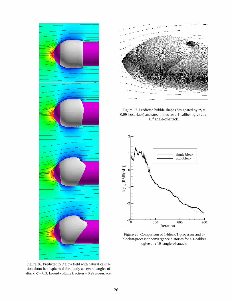
Figure 26. Predicted 3-D flow field with natural cavita-tion about hemispherical fore-body at several angles of

attack. σ = 0.3. Liquid volume fraction = 0.99 isosurface.

Figure 27. Predicted bubble shape (designated by αl = 0.99 isosurface) and streamlines for a 1-caliber ogive at a

10o angle-of-attack.

Iteration

log 10

[RM

S(∆U

)]

0 300 600 900-3

-2

-1

0

1

2

single blockmultiblock

Figure 28. Comparison of 1-block/1-processor and 8-block/8-processor convergence histories for a 1-caliber

ogive at a 10o angle-of-attack.

26

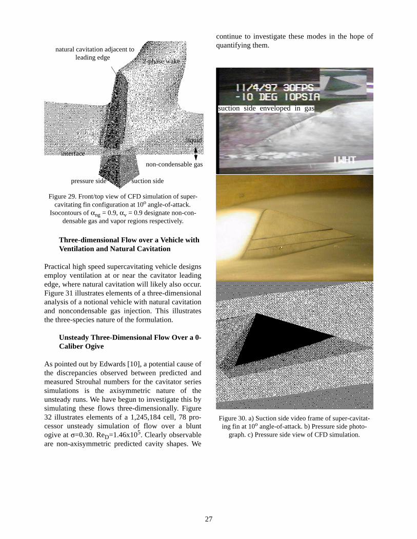
Three-dimensional Flow over a Vehicle with Ventilation and Natural Cavitation

Practical high speed supercavitating vehicle designsemploy ventilation at or near the cavitator leadingedge, where natural cavitation will likely also occur.Figure 31 illustrates elements of a three-dimensionalanalysis of a notional vehicle with natural cavitationand noncondensable gas injection. This illustratesthe three-species nature of the formulation.

Unsteady Three-Dimensional Flow Over a 0-Caliber Ogive

As pointed out by Edwards [10], a potential cause ofthe discrepancies observed between predicted andmeasured Strouhal numbers for the cavitator seriessimulations is the axisymmetric nature of theunsteady runs. We have begun to investigate this bysimulating these flows three-dimensionally. Figure32 illustrates elements of a 1,245,184 cell, 78 pro-cessor unsteady simulation of flow over a bluntogive at σ=0.30. ReD=1.46x105. Clearly observableare non-axisymmetric predicted cavity shapes. We

continue to investigate these modes in the hope ofquantifying them.

pressure side suction side

natural cavitation adjacent toleading edge

interface

2-phase wake

liquid

non-condensable gas

Figure 29. Front/top view of CFD simulation of super-cavitating fin configuration at 10o angle-of-attack.

Isocontours of αng = 0.9, αv = 0.9 designate non-con-densable gas and vapor regions respectively.

suction side enveloped in gas

Figure 30. a) Suction side video frame of super-cavitat-ing fin at 10o angle-of-attack. b) Pressure side photo-

graph. c) Pressure side view of CFD simulation.

27

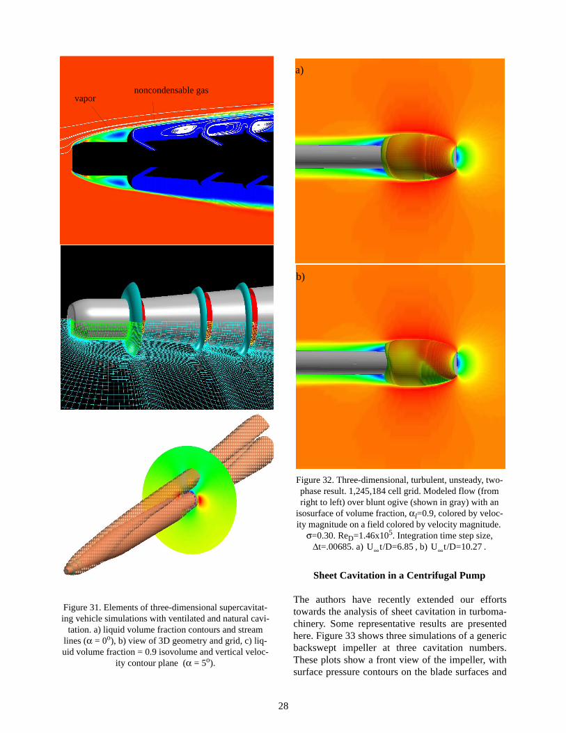
Sheet Cavitation in a Centrifugal Pump

The authors have recently extended our effortstowards the analysis of sheet cavitation in turboma-chinery. Some representative results are presentedhere. Figure 33 shows three simulations of a genericbackswept impeller at three cavitation numbers.These plots show a front view of the impeller, withsurface pressure contours on the blade surfaces and

Figure 31. Elements of three-dimensional supercavitat-ing vehicle simulations with ventilated and natural cavi-

tation. a) liquid volume fraction contours and stream lines (α = 0o), b) view of 3D geometry and grid, c) liq-uid volume fraction = 0.9 isovolume and vertical veloc-

ity contour plane (α = 5o).

vapornoncondensable gas

b)

a)

Figure 32. Three-dimensional, turbulent, unsteady, two-phase result. 1,245,184 cell grid. Modeled flow (from right to left) over blunt ogive (shown in gray) with an

isosurface of volume fraction, αl=0.9, colored by veloc-ity magnitude on a field colored by velocity magnitude.

σ=0.30. ReD=1.46x105. Integration time step size, ∆t=.00685. a) , b) .U∞t/D=6.85 U∞t/D=10.27

28

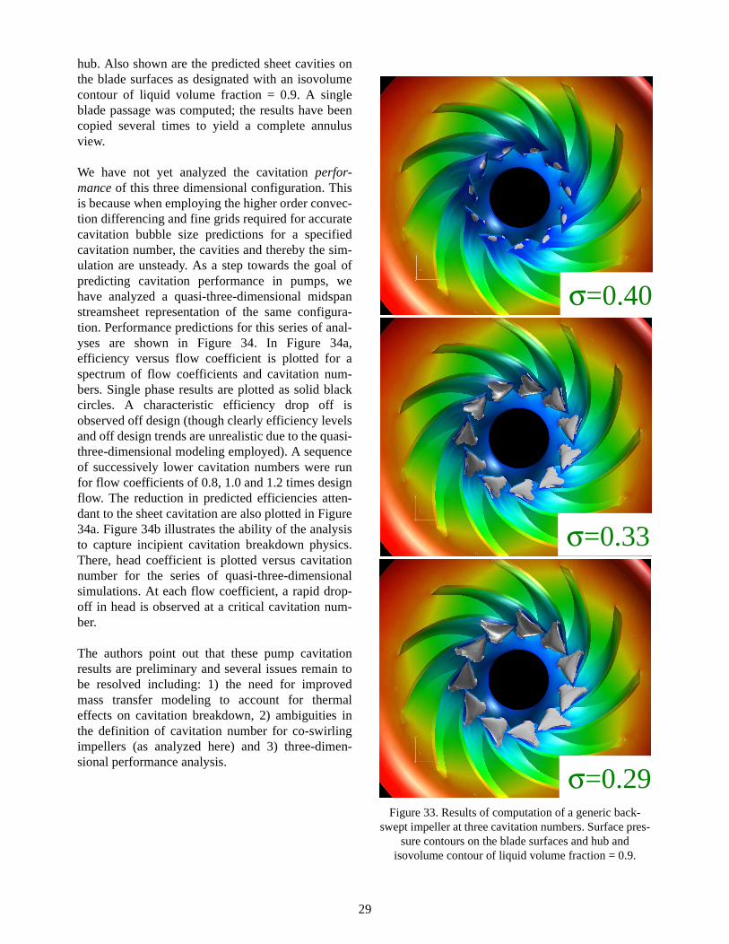
hub. Also shown are the predicted sheet cavities onthe blade surfaces as designated with an isovolumecontour of liquid volume fraction = 0.9. A singleblade passage was computed; the results have beencopied several times to yield a complete annulusview.

We have not yet analyzed the cavitation perfor-mance of this three dimensional configuration. Thisis because when employing the higher order convec-tion differencing and fine grids required for accuratecavitation bubble size predictions for a specifiedcavitation number, the cavities and thereby the sim-ulation are unsteady. As a step towards the goal ofpredicting cavitation performance in pumps, wehave analyzed a quasi-three-dimensional midspanstreamsheet representation of the same configura-tion. Performance predictions for this series of anal-yses are shown in Figure 34. In Figure 34a,efficiency versus flow coefficient is plotted for aspectrum of flow coefficients and cavitation num-bers. Single phase results are plotted as solid blackcircles. A characteristic efficiency drop off isobserved off design (though clearly efficiency levelsand off design trends are unrealistic due to the quasi-three-dimensional modeling employed). A sequenceof successively lower cavitation numbers were runfor flow coefficients of 0.8, 1.0 and 1.2 times designflow. The reduction in predicted efficiencies atten-dant to the sheet cavitation are also plotted in Figure34a. Figure 34b illustrates the ability of the analysisto capture incipient cavitation breakdown physics.There, head coefficient is plotted versus cavitationnumber for the series of quasi-three-dimensionalsimulations. At each flow coefficient, a rapid drop-off in head is observed at a critical cavitation num-ber.

The authors point out that these pump cavitationresults are preliminary and several issues remain tobe resolved including: 1) the need for improvedmass transfer modeling to account for thermaleffects on cavitation breakdown, 2) ambiguities inthe definition of cavitation number for co-swirlingimpellers (as analyzed here) and 3) three-dimen-sional performance analysis.

σ=0.40

σ=0.33

σ=0.29Figure 33. Results of computation of a generic back-

swept impeller at three cavitation numbers. Surface pres-sure contours on the blade surfaces and hub and

isovolume contour of liquid volume fraction = 0.9.

29

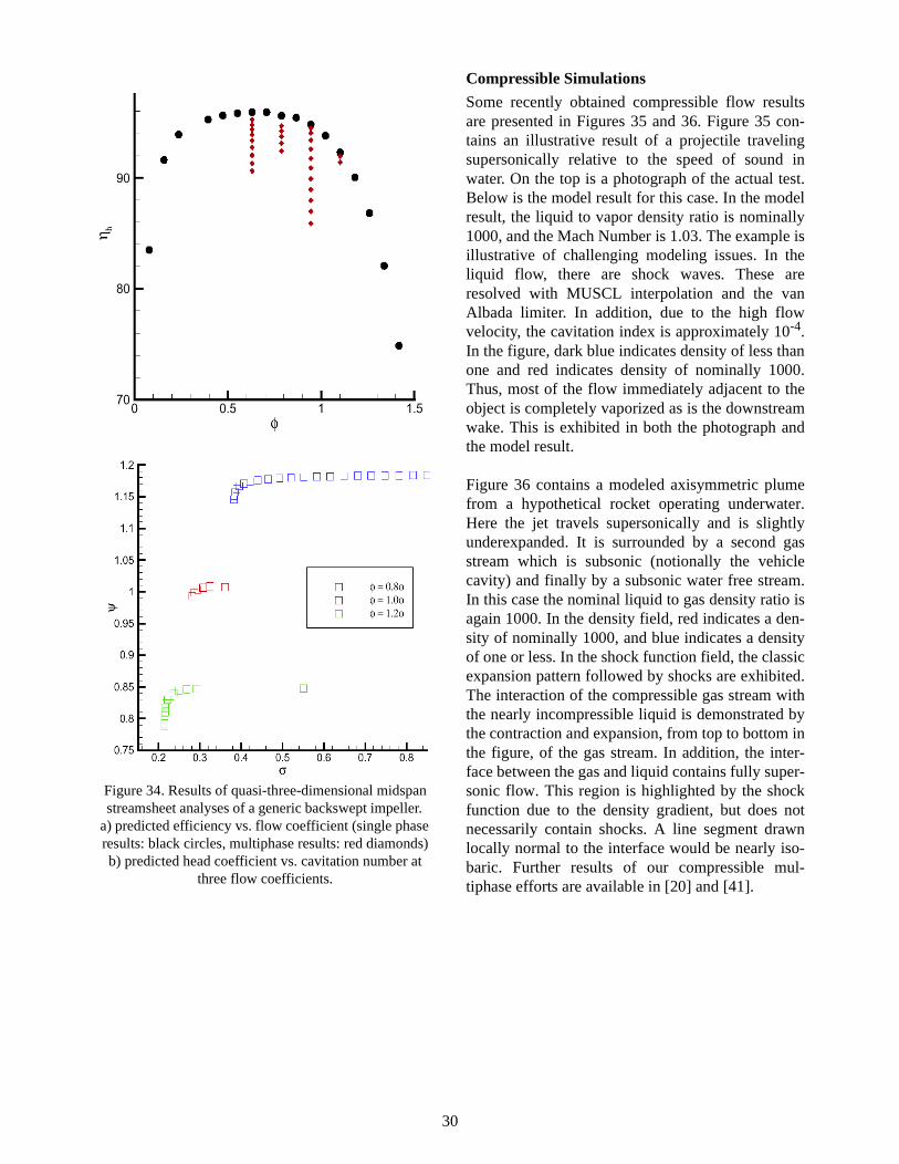
Compressible Simulations

Some recently obtained compressible flow resultsare presented in Figures 35 and 36. Figure 35 con-tains an illustrative result of a projectile travelingsupersonically relative to the speed of sound inwater. On the top is a photograph of the actual test.Below is the model result for this case. In the modelresult, the liquid to vapor density ratio is nominally1000, and the Mach Number is 1.03. The example isillustrative of challenging modeling issues. In theliquid flow, there are shock waves. These areresolved with MUSCL interpolation and the vanAlbada limiter. In addition, due to the high flowvelocity, the cavitation index is approximately 10-4.In the figure, dark blue indicates density of less thanone and red indicates density of nominally 1000.Thus, most of the flow immediately adjacent to theobject is completely vaporized as is the downstreamwake. This is exhibited in both the photograph andthe model result.

Figure 36 contains a modeled axisymmetric plumefrom a hypothetical rocket operating underwater.Here the jet travels supersonically and is slightlyunderexpanded. It is surrounded by a second gasstream which is subsonic (notionally the vehiclecavity) and finally by a subsonic water free stream.In this case the nominal liquid to gas density ratio isagain 1000. In the density field, red indicates a den-sity of nominally 1000, and blue indicates a densityof one or less. In the shock function field, the classicexpansion pattern followed by shocks are exhibited.The interaction of the compressible gas stream withthe nearly incompressible liquid is demonstrated bythe contraction and expansion, from top to bottom inthe figure, of the gas stream. In addition, the inter-face between the gas and liquid contains fully super-sonic flow. This region is highlighted by the shockfunction due to the density gradient, but does notnecessarily contain shocks. A line segment drawnlocally normal to the interface would be nearly iso-baric. Further results of our compressible mul-tiphase efforts are available in [20] and [41].

Figure 34. Results of quasi-three-dimensional midspan streamsheet analyses of a generic backswept impeller.

a) predicted efficiency vs. flow coefficient (single phase results: black circles, multiphase results: red diamonds) b) predicted head coefficient vs. cavitation number at

three flow coefficients.

30

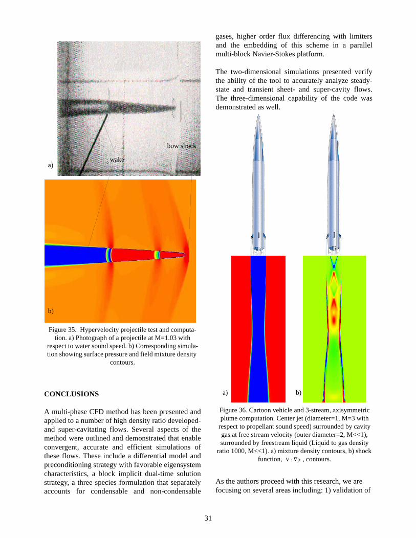
CONCLUSIONS

A multi-phase CFD method has been presented andapplied to a number of high density ratio developed-and super-cavitating flows. Several aspects of themethod were outlined and demonstrated that enableconvergent, accurate and efficient simulations ofthese flows. These include a differential model andpreconditioning strategy with favorable eigensystemcharacteristics, a block implicit dual-time solutionstrategy, a three species formulation that separatelyaccounts for condensable and non-condensable

gases, higher order flux differencing with limitersand the embedding of this scheme in a parallelmulti-block Navier-Stokes platform.

The two-dimensional simulations presented verifythe ability of the tool to accurately analyze steady-state and transient sheet- and super-cavity flows.The three-dimensional capability of the code wasdemonstrated as well.

As the authors proceed with this research, we are focusing on several areas including: 1) validation of

Figure 35. Hypervelocity projectile test and computa-tion. a) Photograph of a projectile at M=1.03 with

respect to water sound speed. b) Corresponding simula-tion showing surface pressure and field mixture density

contours.

bow shock

wakea)

b)

Figure 36. Cartoon vehicle and 3-stream, axisymmetric plume computation. Center jet (diameter=1, M=3 with

respect to propellant sound speed) surrounded by cavity gas at free stream velocity (outer diameter=2, M<<1), surrounded by freestream liquid (Liquid to gas density

ratio 1000, M<<1). a) mixture density contours, b) shock function, , contours.V ρ∇⋅

a) b)

31

the method for compressible constituent fields, 2) improved physical models for mass transfer and tur-bulence, 3) extended application and validation for steady and transient three-dimensional flows and 4) improved error damping through preconditioning and pseudo-time-stepping formulations that locally adapt to problem parameters.

ACKNOWLEDGMENTS

This work is supported by the United States Officeof Naval Research with Dr. Kam Ng as contractmonitor. This work was supported in part by a grantof HPC resources from the Arctic Region Super-computing Center and in part by a grant of SGI Ori-gin 2000 HPC time from the DoD HPC Center,Army Research Laboratory Major Shared ResourceCenter.

REFERENCES

1. Ahuja, V., Hosangadi, A., Ungewitter, R., Dash, S.M. (1999) “A Hybrid Unstructured Mesh Solver for Mutli-Fluid Mixtures, AIAA Paper 99-3330.

2. Anderson, W.K., Thomas, J.L., Van Leer, B. (1986) “Comparison of Finite Volume Flux Vector Splittings for the Euler Equations,” AIAA Journal, Vol. 24, No. 9, pp.1453-1460.

3. Arndt, R., Song, C., Kjeldsen, M., He, J., Keller, A. (2000) “Instability of Partial Cavitation: A Numeri-cal/Experimental Approach”, presented at the 23rd Symposium on Naval Hydrodynamics, Val de Reuil, France.

4. Brennan, C.E., Cavitation and Bubble Dynamics, Oxford University Press, New York, 1995.

5. Brennan, C.E., Hydrodynamics of Pumps, Oxford University Press, England, 1994.

6. Chen, Y., Heister, S.D. (1994) “Two-Phase Modeling of Cavitated Flows,” ASME FED-Vol. 190, pp.299-307.

7. Chorin, A.J. (1967) “A Numerical Method for Solv-ing Incompressible Viscous Flow Problems,” Jour-nal of Computational Physics, Vol. 2, pp. 12-26.

8. Dellanoy, Y., Kueny, J.L. (1990) “Two-phase Flow Approach in Unsteady Cavitation Modeling,” ASME FED-Vol. 98, pp.153-158.

9. Dieval, L., Pellone, C., Arnaud, M. (2000) “Advan-tages and Disadvantages of Different Techniques of Modeling of Supercavitation,” Proceedings of Meet-ing on High Speed Hydrodynamics and Supercavita-tion, Grenoble, France.

10. Edwards, J.R. (2000) Published discussion to refer-ence [19].

11. Garabedian, P.R. ( 1958) “Calculation of Axially Symmetric Cavities and Jets,” Pac. J. of Math 6.

12. Grogger, H.A., Alajbegovic, A., (1998) “Calculation

of the Cavitating Flow in Venturi Geometries Using Two Fluid Model,” ASME Paper FEDSM 98-5295.

13. Hirsch, C. (1990) Numerical Computation of Internal and External Flows, Volume 2, John Wiley and Sons, New York.

14. Jameson, A., Schmidt, W., Turkel, E. (1981) “Numerical Solutions of the Euler Equations by Finite Volume Methods Using Runge-Kutta Time-Stepping Schemes,” AIAA Paper 81-1259.

15. Kirchner, I. N. (2001) “Numerical Modeling of Supercavitating Flows,” VKI Special Course on Supercavitating Flows, February.

16. Jones, W.P., Launder, B.E. (1972) “The Prediction of Laminarization with a Two-Equation Model of Tur-bulence,” International Journal of Heat and Mass Transfer, Vol. 15, pp. 301-314.

17. Kunz, R.F., Siebert, B.W., Cope, W.K., Foster, N.F., Antal, S.P., Ettorre, S.M (1998) “A Coupled Phasic Exchange Algorithm for Three-Dimensional Multi-Field Analysis of Heated Flows with Mass Transfer,” Computers and Fluids, Vol. 27, No. 7, pp. 741-768.

18. Kunz, R.F., Boger, D.A., Stinebring, D.R., Chycze-wski, T.S., Lindau, J.W., Gibeling, H.J., Venkateswa-ran, S., Govindan, T.R. (1999) “A Preconditioned Navier-Stokes Method for Two-Phase Flows with Application to Cavitation Predication,” AIAA Paper 99-3329, also Computers and Fluids, Vol. 29, No. 8, [Nov, 2000], pp. 849-875.

19. Lindau, J.W., Kunz, R.F., Gibeling, H.J. (2000) “Val-idation of High Reynolds Number, Unsteady Multi-Phase CFD Modeling for Naval Applications,” pre-sented at the 23rd Symposium on Naval Hydrody-namics, Val de Reuil, France.

20. Lindau, J.W., Kunz, R.F., Venkateswaran, S., Boger, D.A. (2001) “Application of a Preconditioned, Mul-tiple-Species, Compressible, Navier-Stokes Model to Cavitating Flows”, Submitted to the 4th International Symposium on Cavitation, Pasadena, California, 20-23 June.

21. Lindau, J.W., Venkateswaran, S., Kunz, R.F., Merkle, C.L. (2001) “Development of a Fully-Compressible Multi-Phase Reynolds-Averaged Navier-Stokes Model”, Submitted to the 15th AIAA CFD Confer-ence, Anaheim, California, 11-14 June.

22. May, A. (1975) “Water Entry and the Cavity-Run-ning Behaviour of Missiles,” Naval Sea Systems Command Hydroballistics Advisory Committee TR-75-2.

23. Merkle, C.L., Feng, J., Buelow, P.E.O. (1998) “Com-putational Modeling of the Dynamics of Sheet Cavi-tation,” Proceedings of 3rd International Symposium on Cavitation, Grenoble, France, pp. 307-311.

24. Orszag, S.A., Yakhot, V., Flannery, W.S., Boysan, F., Choudhury, D., Maruzewski, J., Patel, B. (1993) “Renormalization Group Modeling and Turbulence Simulations, Near Wall Turbulent Flows,” Elsevier Science Publishers B.V., Amsterdam, The Nether-

32

lands.25. Reboud, J. L., Delannoy, Y. (1994) “Two-Phase Flow

Modeling of Unsteady Cavitation,” Proceedings of 2nd International Symposium on Cavitation, Tokyo, Japan, pp. 39-44.

26. Reboud, J. L., Fortes-Patella, R., Hofman, M., Lohr-berg, H., Ludwig, G., Stoffel, B. (1999) “Numerical and Experimental Investigations on the Self-Oscillat-ing Behaviour of Cloud Cavitation,” ASME Paper FEDSM99-7259, Proceedings of 3rd ASME/JSME Joint Fluids Engineering Conference.

27. Reichardt, H. (1946) “The Laws of Cavitation Bub-bles at Axially Symmetrical Bodies in a Flow,” Min-istry of Aircraft Production Volkenrode, MAP-VG, Reports and Translations 766, Office of Naval Research.

28. Rogers, S. E., Chang, J. L. C., Kwak, D. (1989) “A Diagonal Algorithm for the Method of Pseudocom-pressibility,” Journal of Computational Physics, Vol. 73, pp. 364-379.

29. Rouse, H., McNown, J. S. (1948) “Cavitation and Pressure Distribution, Head Forms at Zero Angle of Yaw,” Studies in Engineering, Bulletin 32, State Uni-versity of Iowa.

30. Saurel, R., Cocchi, J.P., Butler, P.B. (1999) “Numeri-cal Study of Cavitation in the Wake of a Hyperveloc-ity Underwater Projectile,” AIAA Journal of Propulsion and Power, Vol. 15, No.4, pp. 513-520.

31. Schlichting, H. (1979) Boundary-Layer Theory, McGraw-Hill, New York.

32. Shin, B.R., Ikohagi, T. (1998) “A Numerical Study of Unsteady Cavitating Flows,” Proceedings of 3rd International Symposium on Cavitation, Grenoble, France, pp. 301-306.

33. Shyy, Wei (2000) Personal communication and pub-lished discussion to reference [19].

34. Siebert, B.W., Maneri, C. C., Kunz, R.F., Edwards, D. P. (1995) “A Four-Field Model and CFD Imple-mentation for Multi-Dimensional, Heated Two-Phase Flows,” 2nd International Conference on Multiphase Flows, Kyoto, Japan.

35. Song, C., He, J., (1998) “Numerical Simulation of Cavitating Flows by Single-Phase Flow Approach,” Proceedings of 3rd International Symposium on Cav-

itation, Grenoble, France, pp. 295-300.36. Stinebring, D.R., Billet, M.L., Holl, J.W. (1983) “An

Investigation of Cavity Cycling for Ventilated and Natural Cavities,” TM 83-13, The Pennsylvania State University Applied Research Laboratory.

37. Stinebring, D.R. (1976) “Scaling of Cavitation Dam-age,” M.S. Thesis, The Pennsylvania State Univer-sity, University Park, Pennsylvania, August.

38. Stinebring, D.R., Billet, M.L., Lindau, J.W., Kunz, R.F. (2001) “Developed Cavitation-Cavity Dynam-ics,” VKI Special Course on Supercavitating Flows, February.

39. Taylor, L. K., Arabshahi, A., Whitfield, D. L. (1995) “Unsteady Three-Dimensional Incompressible Navier-Stokes Computations for a Prolate Spheroid Undergoing Time-Dependent Maneuvers,” AIAA Paper 95-0313.

40. Venkateswaran, S., Deshpande, M., Merkle, C.L. (1995) “The Application of Preconditioning to Reacting Flow Computations,” AIAA Paper 95-1673, from Proceedings of the 12th AIAA Computa-tional Fluid Dynamics Conference.

41. Venkateswaran, S., Lindau, J.W., Kunz, R.F., Merkle, C.L. (2001) “Evaluation of Preconditioning Algo-rithms for the Computation of Multi-Phase Mixture Flows,” AIAA Paper 2001-0279.

42. Venkateswaran, S., Merkle, C. L. (1995) “Dual Time Stepping and Preconditioning for Unsteady Compu-tations,” AIAA Paper 95-0078.

43. Van der Heul, D.R., Vuik, C., Wesseling, P. (2000) “Efficient Computation of Flow with Cavitation bay Compressible Pressure Correction”, Proceedings of AMIF-ESF Workshop on Computing Methods for Two-Phase Flow, Aussois, France.

44. Vasin, A. (2000) “High Speed Body Motion in COm-pressible Fluid,” Proceedings of Meeting on High Speed Hydrodynamics and Supercavitation, Greno-ble, France.

45. Whitfield, D. L., Taylor, L. K. (1994) “Numerical Solution of the Two-Dimensional Time-Dependent Incompressible Euler Equations,” Mississippi State University CFD Laboratory Report MSSU-EIRS-ERC-93-14.

33