f.w. klaiber,t.j. wipf, j.r. reid, m.j. peterson
TRANSCRIPT
F.W. Klaiber,T.J. Wipf, J.R. Reid, M.J. Peterson
Investigation of Two Bridge Alternatives for Low Volume Roads
Volume 2 of 2
~~ Iowa Department ~l of Transportation
Concept 2: Beam In Slab Bridge
Sponsored by the Iowa Department of Transportation
Project Development Division and the Iowa Highway Research Board
April 1997
Iowa DOT Project HR-382 ISU-ERl-Ames-97405
---.-College of Engineering
Iowa State University

The opinions, findings, and conclusions expressed in this publication are those of the authors and not necessarily those of the Iowa Department of Transportation

F.W. Klaiber, T.J. Wipf, J.R. Reid, M.J. Peterson
Investigation of Two Bridge Alternatives for Low Volume Roads
Volume 2 of 2
Concept 2: Beam In Slab Bridge
Sponsored by the Iowa Department of Transportation
Project Development Division and the Iowa Highway Research Board
Iowa DOT Project HR-382 ISU-ERl-Ames-97 405
··~en in.earing researc institute
iowa state university
ABSTRACT
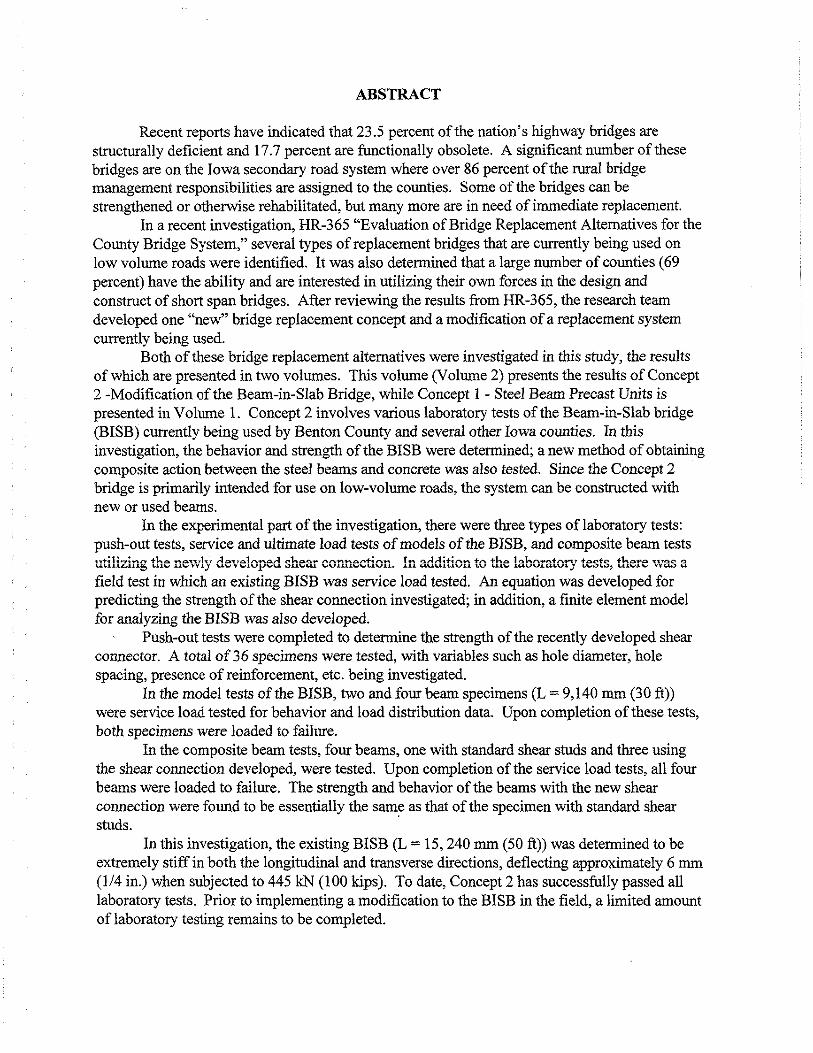
Recent reports have indicated that 23.5 percent of the nation's highway bridges are structurally deficient and 17. 7 percent are functionally obsolete. A significant number of these bridges are on the Iowa secondary road system where over 86 percent of the rural bridge management responsibilities are assigned to the counties. Some of the bridges can be strengthened or otherwise rehabilitated, but many more are in need of immediate replacement.
In a recent investigation, HR-365 "Evaluation of Bridge Replacement Alternatives for the County Bridge System," several types of replacement bridges that are currently being used on low volume roads were identified. It was also determined that a large number of counties ( 69 percent) have the ability and are interested in utilizing their own forces in the design and construct of short span bridges. After reviewing the results from HR-365, the research team developed one "new" bridge replacement concept and a modification of a replacement system currently being used.
Both of these bridge replacement alternatives were investigated in this study, the results of which are presented in two volumes. This volume (Volume 2) presents the results of Concept 2 -Modification of the Beam-in-Slab Bridge, while Concept 1 - Steel Beam Precast Units is presented in Volume 1. Concept 2 involves various laboratory tests of the Beam-in-Slab bridge (BISB) currently being used by Benton County and several other Iowa counties. In this investigation, the behavior and strength of the BISB were determined; a new method of obtaining composite action between the steel beams and concrete was also tested. Since the Concept 2 bridge is primarily intended for use on low-volume roads, the system can be constructed with new or used beams.
In the experimental part of the investigation, there were three types of laboratory tests: push-out tests, service and ultimate load tests of models of the BISB, and composite beam tests utilizing the ne\Vly developed shear corJiection. In addition to Llie laborator; tests, there -.,,vas a field test in which an existing BISB was service load tested. An equation was developed for predicting the strength of the shear connection investigated; in addition, a finite element model for analyzing the BISB was also developed.
Push-out tests were completed to determine the strength of the recently developed shear connector. A total of 36 specimens were tested, with variables such as hole diameter, hole spacing, presence of reinforcement, etc. being investigated.
In the model tests of the BISB, two and four beam specimens (L = 9,140 mm (30 ft)) were service load tested for behavior and load distribution data. Upon completion of these tests, both specimens were loaded to failure.
In the composite beam tests, four beams, one with standard shear studs and three using the shear connection developed, were tested. Upon completion of the service load tests, all four beams were loaded to failure. The strength and behavior of the beams with the new shear connection were found to be essentially the same as that of the specimen with standard shear studs. .
In this investigation, the existing BISB (L = 15, 240 mm (50 ft)) was determined to be extremely stiff in both the longitudinal and transverse directions, deflecting approximately 6 mm (1/4 in.) when subjected to 445 kN (100 kips). To date, Concept 2 has successfully passed all laboratory tests. Prior to implementing a modification to the BISB in the field, a limited amount oflaboratory testing remains to be completed.

v
TABLE OF CONTENTS
ABSTRACT ................................................................. iii
List of Figures . . . . . . . . . . . . . . . . . . . . . . . . . . . . . . . . . . . . . . . . . . . . . . . . . . . . . . . . . . . . . . . ix
List of Tables ............................................................... xiii
l. INTRODUCTION AND LITERATURE REVIEW ............................... l
1.1 Background ........................................................... 1
1.2 Objective and Scope .................................................... 2
1.3 Research Approach ..................................................... 3
1.3.1 Push-out Tests ................................................... 3
1.3.2 BISB Laboratory Tests ............................................. 3
1.3.2.1 Two-Beam Specimen ....................................... 3
1.3.2.2 Four-Beam Specimen ....................................... 4
1.3.3 Composite Specimens ............................................. 4
1.3.4 BISB Field Tests ................................................. 4
1.4 Benton County Bridge .................................................. 5
1.5 Literature Review ...................................................... 9
1.5 .1 Leonhardt, et al. - The Pioneers ...................................... 9
1.5.2 Veldanda, Oguejiofor, and Hosain - Canadian Studies ................... 14
1.5.3 Roberts and Heywood -Australian Studies ............................ 17
2. SPECIMEN DETAILS ..................................................... 21
2.1 Push-out Test Specimens ............................................... 21
2.2 BISB Laboratory Specimens ............................................. 25
2.3 Composite Beam Specimens ............................................. 26
2.3.1 Inverted T-Beam ................................................. 26
2.3.2 Imbedded I-Beam ................................................ 30
2.3.3 Standard Composite Beam ......................................... 34
2.4 BISB Field Bridge .................................................... 34

vi
Page
3. TESTING PROGRAM ..................................................... 41
3.1 Push-out Tests ........................................................ 41
3.2 BISB Laboratory Tests ................................................. 43
3.2.l Two-Beam Specimen ............................................. 43
3.2.2 Four-Beam Specimen ............................................. 47
3.3 Composite Beam Tests ................................................. 53
3.3.l Service Load Tests ............................................... 53
3.3.2 Ultimate Load Tests .............................................. 53
3.4 BISB Field Tests ...................................................... 57
4. BEAM-IN-SLAB BRIDGE GRILLAGE ANALYSIS ............................ 65
4.1 Element Types ....................................................... 65
4.1.1 BEAM4 Element ................................................ 65
4.1.2 BEAM44 3-D Tapered Unsymmetric Beam Element .................... 65
4.2 Grillage Analogy Model ................................................ 66
5. EXPERIMENTAL AND ANALYTICAL RESULTS ............................. 73
5.1 Push-out Test Results and Theoretical Analysis ............................ ; . 73
5. I. I Experimental Results ............................................. 73
5.1.2 Analysis of Experimental Results and Development of Strength Equation .... 80
5. 1.3 Sensitivity Study of Theoretical Strength Equation ...................... 84
5.2 BISB Laboratory Test Results and Analysis ................................ 87
5.2.l Two-Beam Specimen ............................................. 87
5.2.2 Four-Beam Specimen ............................................. 93
5.2.2. l Experimental Results ...................................... 93
5.2.2.2 Comparison of Experimental and Analytical Results ............. IOI
5.3 Composite Beam Test Results .......................................... 104
5.4 Field Bridge Test Results and Analysis ................................... 112
5.4.l Field Bridge Results ............................................. 112
vii
Page
5.4.2 Comparison of Experimental and Analytical Results ................... 124
6. SUMMARY AND CONCLUSIONS ......................................... 131
7. RECOMMENDED RESEARCH ............................................ 135
8. ACKNOWLEDGEMENTS ................................................ 138
9. REFERENCES .......................................................... 139
ix
LIST OF FIGURES
Page
Fig. 1.1. Beam-in-slab bridge ................................................... 6
Fig. 1.2. Photographs ofBISB applications ........................................ 7
Fig. 1.3. BISB abutment detals .................................................. 8
Fig. 1.4. Leonhardt's Perfobond Rib Connector .................................... 10
Fig. 1.5. Internal forces in a composite beam associated with the Perfobond Rib
Shear Connector . . . . . . . . . . . . . . . . . . . . . . . . . . . . . . . . . . . . . . . . . . . . . . . . . . . . . 12
Fig. 1.6. Inverted steel T-section with perforbond rib shear connectors .................. 19
Fig. l.7. RobertsandHeywood'sshearboxtest .................................... 19
Fig. 2.1. Push-out specimens ................................................... 22
Fig. 2.2. Description of the hole arrangements used in the push-out tests ................ 23
Fig. 2.3. Cross section ofBISB four-beam specimen ................................ 27
Fig. 2.4. Composite beam specimen: T-section (Specimen 1) ......................... 28
Fig. 2.5. T-section fabrication cutting schedule ..................................... 31
Fig. 2.6. Composite beam specimen: Imbedded I-beam (Specimens 2 and 3) ............. 32
Fig. 2.7. Composite beam specimen: Welded studs (Specimen 4) ...................... 35
Fig. 2.8. Description of field bridge .............................................. 37
Fig. 2.9. Photograph ofBISB bridge tested ........................................ 39
Fig. 3.1. Location of instrumentation used in the push-out tests .............. : ......... 42
Fig. 3.2. Loading apparatus used for testing the BISB two-beam specimen ............... 44
Fig. 3.3. Instrumentation for the two-beam specimen ................................ 46
Fig. 3.4. Location of strain gages on four-beam specimen ............................ 48
Fig. 3.5. Location of strain gaged cross sections on four-beam specimen ................ 49
Fig. 3.6. Location ofloading points for service level load testing the four-beam specimen ... 50
Fig. 3.7. Locations ofload points for ultimate load test of the four-beam specimen ........ 52
Fig. 3.8. Location of strain gages on composite beam specimens ....................... 54
Fig. 3.9. Location of deflection instrumentation in composite beam tests ................ 55
Fig. 3.10. Composite beam test setup ............................................. 56
x
Page
Fig. 3.11. Location of instrumentation- field bridge .................................. 58
Fig. 3.12. Wheel configuration and weight distribution oftest vehicles ................... 60
Fig. 3.13. Location oftest vehicles ............................................... 61
Fig. 3.14. Photographs oftest vehicles on bridge .................................... 62
Fig. 4.1. Geometry ofBEAM4 element. ............... ; .......................... 66
Fig. 4.2. Geometry ofBEAM44 element .......................................... 66
Fig. 4.3. Basic gri!lage model ofBISB system ..................................... 68
Fig. 4.4. Sensitivity study results for basic parameters ............................... 70
Fig. 4.5. Sensitivity studies for beam properties .................................... 72
Fig. 5.1. Load slip curves for various test sequences ....................... .' ........ 77
Fig. 5.2. Illustration of equation variables ......................................... 82
Fig. 5.3. Shear strength vs. hole area ............................................. 86
Fig. 5.4. Shear strength vs. area ofreinforcing steel through shear hole .................. 86
Fig. 5.5. Shear strength vs. area of transverse reinforcement .......................... 88
Fig. 5.6. Shear strength vs. number of shear holes .................................. 88
Fig. 5. 7. Strain response for two-beam BISB during load testing ....................... 90
Fig. 5.8. Strain profile for two-beam BISB during load testing ........................ 91
Fig. 5.9. Average end slip during load testing ...................................... 92
Fig. 5.10. Theoretical and experimental midspan deflection ............................ 92
Fig. 5.1 l. Test Al results: deflections and strains at centerline ......................... 95
Fig. 5.12. Deflection of beams due to 20 kips load applied at Section l ................... 96
Fig. 5.13. Deflection of beams due to 20 kips load applied at Section 2 ................... 97
Fig. 5.14. Deflection of beams due to 20 kips load applied at Section 3 ................... 98
Fig. 5.15. Deflections during BISB ultimate load test ................................. 99
Fig. 5.16. Strains during ultimate load test ........................................ 100
Fig. 5.17. Comparison of experimental and analytical results for BISB Test Al ........... 102
Fig. 5.18. Comparison of experimental and analytical results for BISB Test C3 ........... 103
J
)
)
)
)
)
)
)
xi
Page
Fig. 5.19. Specimen 1 service test results ......................................... 105
Fig. 5.20. Specimen 2 service test results ......................................... 106
Fig. 5.21. Comparison of service test results of Specimens 2 and 3 ..................... 108
Fig. 5.22. Specimen 3 service test results ......................................... 109
Fig. 5.23. Specimen 4 service test results ......................................... 110
Fig. 5 .24. Comparison of the composite beam deflection at the centerline ................ 111
Fig. 5.25. Ultimate load deflections .............................................. 113
Fig. 5.26. Deflection and moment fraction data for Test 1 ............................ 114
Fig. 5.27. Deflection and moment fraction data for Test 2 ............................ 115
Fig. 5.28. Deflection and moment fraction data for Test 3 ............................ 116
Fig. 5.29. Deflection and moment fraction data for Test 4 ............................ 117
Fig. 5.30. Deflection and moment fraction data for Test 5 ............................ 118
Fig. 5.31.Deflection and moment fraction data for Test 6 ............................ 119
Fig. 5.32. Deflection and moment fraction data for Test 7 ............................ 120
Fig. 5.33. Deflection and moment fraction data for Test 8 ............................ 121
Fig. 5.34. Symmetry determination on field bridge .................................. 123
Fig. 5.35. Field bridge grillage analogy ........................................... 125
Fig. 5.36. Comparison of theoretical and experimental deflections at midspan: Test 1 ...... 126
Fig. 5.37. Comparison of theoretical and experimental deflections at midspan: Test 2 ...... 126
Fig. 5.38. Comparison of theoretical and experimental deflections at midspan: Test 3 ...... 127
Fig. 5.39. Comparison of theoretical and experimental deflections at midspan: Test 4 ...... 127
Fig. 5.40. Comparison of theoretical and experimental deflections at midspan: Test 5 ...... 128
Fig. 5.41. Comparison of theoretical and experimental deflections at midspan: Test 7 ...... 128
Fig. 5.42. Comparison of theoretical and experimental deflections at midspan: Test 8 ...... 129
Fig. 5.43 Comparison of theoretical and experimental moment fractions at midspan:
Test 2, truck at midspan .............................................. 129
Fig. 5.44 Comparison of theoretical and experimental moment fractions at midspan:
Test 7, truck at midspan .............................................. 130

xiii
LIST OF TABLES
Page
Table 2.1. Beam spacing in field bridge .......................................... 38
Table 2.2. Field bridge abutment measurements .................................... 38
Table 3.1. Test designations for BISB field tests ................................... 63
Table 5.1. Push-out test results ................................................. 75
Table 5.2. Theoretical strengths vs. experimental strengths ........................... 84
Table 5.3. Results of sensitivity investigation ...................................... 85
1. INTRODUCTION AND LITERATURE REVIEW
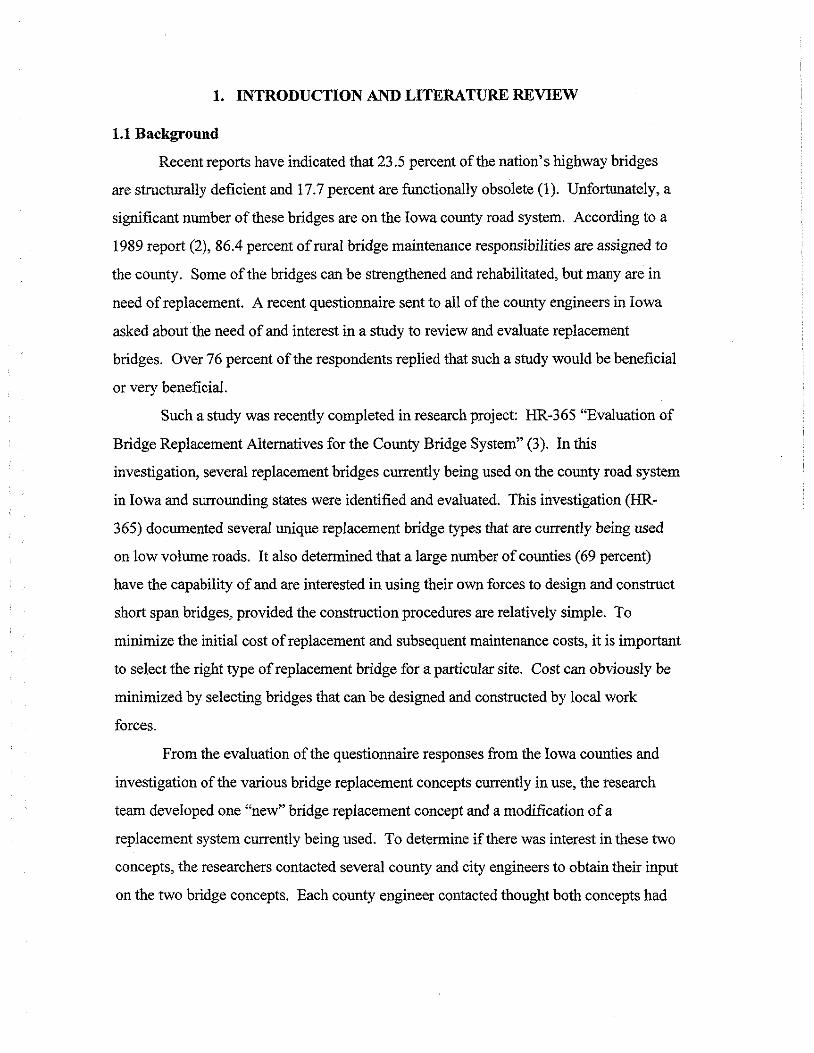
1.1 Background
Recent reports have indicated that 23.5 percent of the nation's highway bridges
are structurally deficient and 17.7 percent are functionally obsolete (1). Unfortunately, a
significant number of these bridges are on the Iowa county road system. According to a
1989 report (2), 86.4 percent of rural bridge maintenance responsibilities are assigned to
the county. Some of the bridges can be strengthened and rehabilitated, but many are in
need of replacement. A recent questionnaire sent to all of the county engineers in Iowa
asked about the need of and interest in a study to review and evaluate replacement
bridges. Over 76 percent of the respondents replied that such a study would be beneficial
or very beneficial.
Such a study was recently completed in research project: HR-365 "Evaluation of
Bridge Replacement Alternatives for the County Bridge System" (3). In this
investigation, several replacement bridges currently being used on the county road system
in Iowa and surrounding states were identified and evaluated. This investigation (HR-
365) documented several unique replacement bridge types that are currently being used
on low volume roads. It also determined that a large number of counties (69 percent)
have the capability of and are interested in using their own forces to design and construct
short span bridges, provided the construction procedures are relatively simple. To
minimize the initial cost of replacement and subsequent maintenance costs, it is important
to select the right type of replacement bridge for a particular site. Cost can obviously be
minimized by selecting bridges that can be designed and constructed by local work
forces.
From the evaluation of the questionnaire responses from the Iowa counties and
investigation of the various bridge replacement concepts currently in use, the research
team developed one "new" bridge replacement concept and a modification of a
replacement system currently being used. To determine ifthere was interest in these two
concepts, the researchers contacted several county and city engineers to obtain their input
on the two bridge concepts. Each county engineer contacted thought both concepts had
2
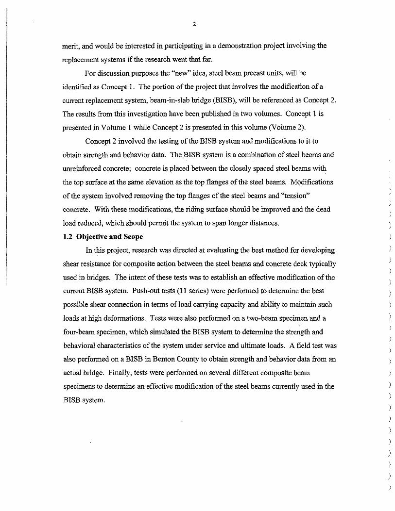
merit, and would be interested in participating in a demonstration project involving the
replacement systems ifthe research went that far.
For discussion purposes the "new" idea, steel beam precast units, will be
identified as Concept 1. The portion of the project that involves the modification of a
current replacement system, beam-in-slab bridge (BISB), will be referenced as Concept 2.
The results from this investigation have been published in two volumes. Concept 1 is
presented in Volume I while Concept 2 is presented in this volume (Volume 2).
Concept 2 involved the testing of the BISB system and modifications to it to
obtain strength and behavior data. The BISB system is a combination of steel beams and
unreinforced concrete; concrete is placed between the closely spaced steel beams with
the top surface at the same elevation as the top flanges of the steel beams. Modifications
of the system involved removing the top flanges of the steel beams and "tension"
concrete. With these modifications, the riding surface should be improved and the dead
load reduced, which should permit the system to span longer distances.
1.2 Objective and Scope
In this project, research was directed at evaluating the best method for developing
shear resistance for composite action between the steel beams and concrete deck typically
used in bridges. The intent of these tests was to establish an effective modification of the
current BISB system. Push-out tests (11 series) were performed to determine the best
possible shear connection in terms ofload carrying capacity and ability to maintain such
loads at high deformations. Tests were also performed on a two-beam specimen and a
four-beam specimen, which simulated the BISB system to determine the strength and
behavioral characteristics of the system under service and ultimate loads. A field test was
also performed on a BISB in Benton County to obtain strength and behavior data from an
actual bridge. Finally, tests were performed on several different composite beam
specimens to determine an effective modification of the steel beams currently used in the
BISB system.
)
)
)
)
)
)
)
)
)
)
)
)
)
)

3
1.3 Research Approach
This study is comprised of four distinct phases: push-out tests, laboratory BISB
specimen tests, composite beam tests, and BISB field tests. Following is a summary of
the tasks perfonned in each phase.
1.3.l Push-out Tests
Based upon the research initially performed by Leonhardt et al. ( 4), eleven series
of push-out specimens were tested to detennine the load carrying capacity and the ability
of the connection to maintain that load over large displacements. Typically, in composite
construction, some type of shear connection on the top flange of the beam is used to
ensure the load is properly transferred from the concrete to the steel. In this investigation,
holes were drilled in the steel web (in beams without a top flange) to provide the
necessary shear connection; this type of shear connection will be referred to as an
alternate shear connector (ASC) in this report. Five variables were evaluated to
detennined the best arrangement of those holes in the ASC:
• Size of holes
• Spacing of holes
• Alignment of holes
• Inclusion of reinforcing steel in holes
• Effects of "sloppy" craftsmanship
The results from these tests were used in designing the ASC, which was in turn used in
the composite beam tests that were subsequently performed.
1.3.2 BISB Laboratory Tests
1.3.2.1 Two-Beam Specimen
Tests were perfonned on a two-beam section modeled after the BISB to obtain
data on its strength and behavior. These tests were completed to detennine the following:
• Load carrying capacity
• Reserve strength after overloading
• Deflections, strains, and slip data during service and ultimate loading
4
1.3.2.2 Four-Beam Specimen
Tests were performed also on a four-beam model of the BISB. The bridge model
was instrumented so that strains and deflections could be determined at critical locations.
The tests were undertaken to determine the following:
• Load distribution in the system
• Behavior under service loads
• Load carrying capacity
• Reserve strength after overloading
• Strains, slip data, and deflections during service and ultimate loading
1.3.3 Composite Specimens
The ASC developed and tested in the push-out tests was used in composite beam
tests. Four composite beams were tested; one had standard shear studs, and the other
three had different variations of the ASC. The composite beams were instrumented so
that strains and deflections could be determined at critical locations. Tests on the
composite beams were completed to determine the amount of composite action, the
behavior under service loads, the ultimate strength, and the type of failure that would
occur when overloaded.
l.3.4 BISB Field Tests
To obtain strength and behavior data from an existing bridge, a BISB in Benton
County was instrumented and tested. The BISB tested was 15,240 mm (50 ft) in length,
had W12 sections, and had no guardrails or gravel cover. Stream conditions, height
above stream, and road conditions were considered in the selection of the test bridge.
Two standard tandem-axle county trucks, with approximate total weights of
222.5 kN (50 kips) each, were used in the testing of the bridge. The trucks were
positioned at critical locations on the bridge to produce maximum strains and deflections.
These data were then compared to theoretical data to determine the amount of composite
action and load distribution in the bridge.
)
)
)

5
1.4 Benton County Bridge
The BISB is a bridge system (see Fig. 1.1) consisting of a series of W shape steel
beams generally spaced at 610 mm (2 ft). These structures are used for spans between
6, I 00 and 15 ,200 nun (20 and 50 ft). In general, this sytem is used on low volume roads.
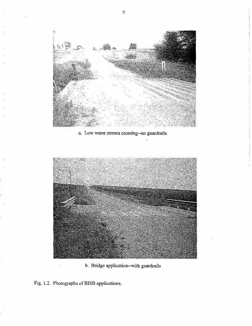
When it is used as a low water stream crossing (see Fig. l .2a), no guardrails are used. At
sites where there are long distances from the bridge deck to the stream, guardrails are
added (see Fig. l.2b).
Typically, nine steel piles are driven on 1,220 mm ( 4 ft) centers in each face of the
two bridge abutments. As shown in Fig. 1.3a, wing walls of the desired height are
connected with reinforcement to each of the abutments. Dowels (see Fig. l.3b) are
provided for connection of the superstructure to the abutment.
The superstructure consists ofa series ofW sections (usually W 12X79)
positioned adjacent to each other on 610 mm (2 ft) centers. The exterior beam is either a
channel section (generally C12X30) of the same height as the W sections, or another W
section. Plywood 16 nun or 19 mm (5/8 in. or 3/4 in.) thick is then placed between the
adjacent beams. The plywood is cut to a width of 460 mm (18 in.) so that when concrete
is placed, it is in contact with the top surface of the bottom flange. Therefore, even after
the formwork has deteriorated, there will still be bearing between the concrete and steel
(see Fig. I.lb). To ensure no movement of the beams during the placement of the
concrete, 6 mm (114 in.) steel straps are welded across the bottom of the flanges at third
points (see Fig. l.3b). Concrete is poured flush with the top flange of the beams. Note,
there is no reinforcement in the concrete. Guardrails may be added by welding posts
(MC 8X22.8) to the exterior channel sections.
In general, as the BISB span length decreases, the cost per square ft. increases. In
1993, a low water stream crossing, spanning 10,400 mm (34 ft) with a width of9,150 mm
(30 ft), was constructed in Blackhawk County at a cost of$35 per square ft. This cost
included guardrails, steel, labor, and equipment rental. Similarly, a 7,600 nun (25 ft)
span bridge without guardrail had a unit cost of$35 per square ft, a 6,400 nun (21 ft) span
cost $42.50 per square ft, and a 12,200 mm (40 ft) bridge was estimated at $32 per
square ft.

6
30' to 50'
I"' W 12x77 / Cl2x30
I• ' ..,..... •
·'-
l/2"x!2"x30' Plate
concrete-
. . ~ /. I>
- /) 6. ·' ..
. . ~ .!'. /. !> - /) 6.• ..
_ plywood forms
Fig. 1.1. Beam-in-slab bridge.
a. Plan view
W 12 x 77 steel beams
1 .. 2' Typical ..1
bearing elevation
b. Cross section
T
30'
. . ~ b /. I>
- /) 6.• ..
)
)
)
)
)
)
7
a. Low water stream crossing--no guardrails
b. Bridge application--with guardrails
Fig. 1.2. Photographs ofBISB applications.

• • • • • • • • • • • • • • • • •
6 ' I
T '
18"
8
reinforcing rods @ 12"
steel piles
0 0 0 cD 0 I
8 spaces@ 4'!= 32'
34'
a: Plan view of abutment
112" x 12" x 36' plate welded to top and bottom of beams and channel flanges
0
314" plywood
9"
~'---- #8 reinforcing bars, 2' long
6" I
b. Connection of superstructure to abutment
Fig. 1.3. BISB abutment details.
12'
0
114 "x 2 "x 30' steel straps welded to beams at third points for bracing
)
)
)
)
)
)
)
)
)
)
)
)
)
)

9
1.5 Literature Review
To the authors' knowledge, the BISB is unique to Iowa. Although several
literature searches (Transportation Research Information Service through the Iowa
Department of Transportation, Geodex System in the ISU Bridge Engineering Center
Library, and several computerized literature searches through the ISU Library) were
made, no information was found on the BISB. Literature review in this investigation
focused on a new means of obtaining shear connection between concrete and steel,
known as the Perfobond Rib Connector. Research has been performed on the Perfobond
Rib Connector in West Germany, Australia, and Canada; however, the literature search
uncovered no research on this type of connector in the United States. In the following
sections, research on this connection undertaken in these three countries is briefly
summarized.
1.5 .1 Leonhardt et al. - The Pioneers
Most composite bridges utilize shear studs as the mechanism for transferring
shear from the concrete to the steel beams. Research over the past 30 years has
determined that over time, due to large local pressures at the foot of the stud, loosening
may occur. This may lead to progressive slippage, resulting in the stresses moving
upward from the foot of the stud. This in turn increases the flexural stress in the stud,
which may result in a flexural failure of the stud. The progressive slippage that starts
this cycle is often the result of fatigue problems. Thus, a shear connector that will be
virtually slip-free is needed, eliminating the possibility for fatigue problems, and
involving only elastic deformations under service loading conditions.
In hopes of overcoming these potential fatigue problems in designing the Third
Caroni Bridge in Venezuela, the consulting firm of Leonhardt, Andrea, and Partners
utilized a new type of shear connector, the Perfobond Rib (see Fig. 1.4). The Perfobond
Rib is a flat rectangular steel plate perforated with a series of holes. The rib is then
welded onto the top flange of a steel beam. The holes are spaced closely, and the
diameter of the holes is greater than the maximum diameter of the coarse aggregate used
in the concrete. This allows the aggregate to penetrate the holes and form a series of

10
transverse reinforcing bar
top flange of I- beam
steel plate
a. Perfobond Rib detail
15 in. Typ. 15.75 in. Typ.
I'" ·I.. ·I
b. Perfobond Rib placement on steel beam
Figure 1.4. Leonhardt's Perfobond Rib Connector.
)
)
)
)
)
)
)
)
)
)
)

11
concrete dowels which act in shear. Steel reinforcement may or may not be included in
the holes depending on the required strength.
With the Perfobond Rib Connector, three types of failure were noted by
Leonhardt et al. There may be a shearing of the steel strip between the Perfobond holes, a
bearing failure of the concrete dowels within the holes, or a shearing failure of the
concrete dowels themselves. Perfobond Ribs are designed to ensure that the concrete
dowels fail in shear. Designating a minimum hole spacing prevents shearing of the steel;
specifying a minimum thickness of steel and minimum amount of transverse
reinforcement ensures the confinement of the concrete, thus preventing a bearing failure.
The transverse reinforcement is needed to confine the concrete around the rib and to
ensure that the concrete in the hole is confined in three dimensions. A strut-tie analogy,
shown in Fig. 1.5, was later used by Roberts and Heywood (5) to explain how the
transverse reinforcement confines the concrete in three dimensions. Without the
transverse reinforcement, the concrete in the holes would tend to "pop out" at relatively
low loads. Transverse reinforcement creates a tensile force that confines the concrete in
the holes, thereby preventing "pop out" failures.
Thus, with proper transverse reinforcement, spacing of the holes, and rib
thickness, stresses in the dowels are below the elastic limit, and a rigid, generally slip
free connection is maintained throughout service level conditions. With increased
loading, the concrete dowel will incur greater shearing stresses, until it fails in shear
along the steel-concrete interface; however, a significant amount of strength will be
maintained due to high levels of friction between the concrete and steel. Failures are
therefore gradual, and in most situations are noticed and can most likely be repaired
before severe damage or failure occurs.
Leonhardt et al. performed a series of three push-out tests, including static and
dynamic loading. Results from these tests led Leonhardt and his colleagues to conclude
the following:
• Low amounts of flexible plastic slip occur between the concrete and steel
during static loading.

12
• There is practically no increase in slip resulting from appplying dynamic
loading rather than static loading.
• After shear failure of the concrete dowels occurred, there was no sudden
decrease in load.
• The most efficient combination of variables tested included holes 35 mm (1.4
in.) in diameter, on 50 mm (2 in.) centers, with a plate thickness of 12 mm
(0.5 in.).
steel tension ties
"'------ concrete compressive struts
Fig. 1.5. Internal forces in a composite beam associated with the Perfobond Rib Shear Connector.
The Perfobond Ribs performed as expected; there was virtually no deformation
llllder static or service loading, no fatigue problems due to dynamic loading, and after
failure, the load was adequately maintained. Based on the test results, design equations
were developed to determine the hole size, spacing, thickness, and amollllt of transverse
reinforcement necessary for adequate strength. ·
As previously noted, three potential failure modes were determined by Leonhardt,
et. al.; details on these three follow. Note that the original equations utilized concrete
cube strength; the following equations were modified to convert the cubic concrete
strength to the more conventional cylinder strength. In addition to the three equations for
)
)
)
)
)
)
)
)
J

13
detennining the ultimate shear, V0 , associated with the three potential types of failure, an
equation was developed for detennining the amount of reinforcing steel required to insure
the concrete inside the hole is confined in three dimensions.
1. Failure of the concrete dowels
7tD2 V0 =2x 4 X l.625fc (1.1)
where:
V 0 = ultimate shear strength for one dowel with two shear
planes, kN.
D = hole diameter, mm.
( = concrete cylinder strength, kPa.
2. Bearing failure of the concrete dowels in the holes
V0 =D x tx 10.?lfc,
where:
t = thickness of the steel plate, mm.
3. Shearing of the steel strip between the holes
f V 0 =A,x .Js X 1C
where:
A,= area of steel in between adjacent holes, mm2•
f,y = yield stress of the steel plate, kPa.
4. Transverse reinforcing requirements
where:
(1.2)
(1.3)
(1.4)
A,1 = Area of transverse steel required per hole, mm2•
As previously noted, the desired failure mode is shearing of the concrete dowels;
therefore, Eqn. I. I is the equation of most interest. The 'two' in Eqn. I. J is due to two
shearing planes, one on each side of the dowel. The area of the hole is then multiplied,
14
along with a factor, times the concrete strength. This factor in the paper by Leonhardt et
al. (4) (based on laboratory tests) was 1.3; however, the 1.625 takes into account the
conversion from cubic strength to cylinder strength. It must be noted that this design
equation is valid only for a steel plate thickness of 12 mm (0.5 in.). Likewise, the
equation is based on pushout tests utilizing only 35 and 40 mm (1.4 and 1.6 in.) holes on
50 mm (2 in.) centers. Furthermore, the equation fails to incorporate the friction or
cohesion between the concrete and the steel plate. Therefore, this design equation is
limited in its application, and cannot be used for significantly different hole spacings and
plate thicknesses.
1.5.2 Veldanda, Oguejiofor, and Hosain - Canadian Studies
Although Leonhardt' s research was completed in 1987, additional research was
not performed until the early l 990's. At that time, researchers at the University of
Saskatchewan began a comprehensive, three phase research program to determine the
feasibility of using the Perfobond Rib Connectors in composite floor systems.
Preliminary investigation by Antunes (6) involved the testing of eight push-out
specimens, and resulted in the recommendation that the height of the Perfobond Rib
Connectors be maximized to obtain the maximum load carrying capacity.
From this preliminary data, Veldanda and Hosain (7) performed a series of 56
push-out tests on various types of Perfobond Ribs. These tests resulted in the following
observations:
• Failure was triggered by the longitudinal splitting of the concrete slab,
followed by the crushing of concrete in front of the Perfobond Rib.
• A considerable amount ofload was retained over a large slip after the
maximum load was attained.
• After failure of the dowels and crushing of the concrete, friction between the
cracked concrete surfaces continued to provide shear resistance.
• The capacity of one Perfobond hole, 35 mm (1.4 in.) diameter, is equivalent to
approximately five 16 mm x 75 mm (0.6 in. x 3 in.) studs.
)
)
)
)
)
)
)
)
)
)
)
)

15
• An appreciable improvement in the shear capacity of the connection was
observed with the addition of steel reinforcement through the Perfobond Rib
holes (approximately, a 50% increase in strength).
• The Perfobond Rib Connectors exhibited greater stiffness under service loads
than conventional headed studs.
• A significant portion of the ultimate shear resistance of a Perfobond Rib
Connector is provided by the concrete dowels.
• "Shallow" Perfobond Rib Connectors ( < 60 mm (2.35 in.) in height) are
relatively ineffective.
• Perfobond Rib Connectors can be effectively used in composite beams with
or without ribbed decks placed parallel to the steel beams.
Phase two of this project involved the verification of the findings from the push
out tests. Oguejiofor and Hosain (8) tested six full-sized composite beams. Three of the
specimens had headed studs, whereas the other three had Perfobond Rib Connectors. In
addition to verifying the push-out test results, the influence of the slab and deck on the
performance of the beams was determined. The span length was held constant, while the
concrete slab width and deck type were varied. Although reinforcing bars were used in
many of the push-out tests, the full size tests utilized only the Perfobond Rib Connectors.
Results of the investigation follow:
• The failure mode observed was longitudinal splitting of the concrete, followed
by concrete crushing in front of the Perfobond Rib Connectors.
• More Perfobond Rib Connectors of smaller size result in a delay of the
concrete crushing and a higher ultimate load.
• All specimens showed excellent ductile behavior.
• The predicted ultimate strength based on push-out tests compared reasonably
well with the experimental values.
The overall conclusion from these papers was that the Perfobond Rib Connector
was a viable alternative to the headed studs currently used in composite bridge
16
construction. Subsequently, the final phase of the study was to investigate the properties
of the Perfobond Rib Connector to establish design guidelines for calculating its capacity
(9). This involved the testing of 42 push-out specimens with variances in reinforcing,
positioning of the Perfobond holes, number of Perfobond holes, and concrete strength.
From these results, an empirical design equation was developed incorporating all the
pertinent terms relating to the strength of the connection. Results of the extensive push
out tests were as follows:
• Failure was initiated by longitudinal splitting of the concrete slab while the
Perfobond Rib Connectors and weld metal remained completely intact.
• Failure occurred in both slabs of the specimens with reinforcing bars.
• An increase in strength was noted for an increase in hole spacing up to
approximately two times the hole size diameter.
• Four holes within a 375 mm (14.75 in) length did not perform as well as three
holes within the length. This is likely due to the overlapping of the stress
fields as the hole spacing decreases.
From these observations, and from a base equation presented by Davies in 1969
(I 0) developed through studying the shear capacity of a stud connector with a similar
failure mechanism, an empirical relationship was developed using the shear area of the
concrete, the area of transverse reinforcement, and the Perfobond hole area.
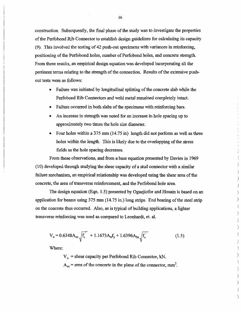
The design equation (Eqn. 1.5) presented by Oguejiofor and Hosain is based on an
application for beams using 375 mm (14.75 in.) Jong strips. End bearing of the steel strip
on the concrete thus occurred. Also, as is typical of building applications, a lighter
transverse reinforcing was used as compared to Leonhardt, et. al.
Vu =0.6348A00.Jf + l.1673AJy + l.6396Ahs.Jr: (1.5)
Where:
Vu =shear capacity per Perfobond Rib Connector, k:N.
Ace= area of the concrete in the plane of the connector, mm2•
)
)
)
)
)
)
)
)
17
Ari= area of transverse reinforcement, mm2•
fy = yield strength of transverse reinforcement, k:Pa.
Ah,= total area of the dowels in shear, mm2•
r« = concrete compressive cylinder strength, k:Pa.
The first term relates to the splitting of the concrete upon failure. The second
term corresponds to the degree of confinement provided by the transverse reinforcement,
and the last term denotes the shear strength of the actual concrete dowel. Due to the
difference in transverse reinforcement used, the failure modes differed, which explains
why Leonhardt, et. al. used the concrete strength while Oguejiofor and Hosain used the
square root of the concrete strength.
To verify the applicability of the empirical relationship to full size beams, five full
size composite beams were also tested. Earlier research has determined that, in general,
results from push-out specimens are conservative compared to those obtained from beam
tests. Slutter and Driscoll (11) attributed the difference to the eccentricity ofloading that
often occurs in push-out specimen. In addition, a greater amount of reinforcement is
required for the push-out specimens to obtain similar ultimate strength of connections
than would be required in a beam. Whatever the case, it has been shown many times that
the results from a push-out test can be used as a conservative estimate of the results of a
similar beam test. Therefore, by comparing the empirical relationship derived from the
push-out results to the data from the beam tests, the empirical relationship can be verified.
Results of that comparison yielded values generally 5%-10% lower than predicted values;
thus, the empirical relationship was assumed to be an accurate strength estimate for
composite beams.
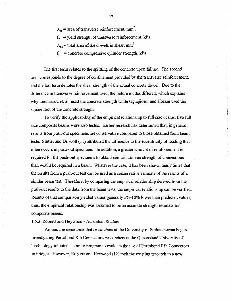
1.5.3 Roberts and Heywood-Australian Studies
Around the same time that researchers at the University of Saskatchewan began
investigating Perfobond Rib Connectors, researchers at the Queensland University of
Technology initiated a similar program to evaluate the use of Perfobond Rib Connectors
in bridges. However, Roberts and Heywood (12) took the existing research to a new
18
level with the idea of removing the top flange of the beam and drilling the holes directly
into the web, creating an inverted steel T-section as shown in Fig. 1.6.
The main purpose of the top flange when the Perfobond Rib Connection is used is
to provide an area on which to weld the steel plate. In terms of strength, the top flange
contributes very little to the composite section due to its close proximity to the neutral
axis. The removal of the top flange not only saves money in material costs, but also
decreases the overall dead weight of the structure, thus allowing the system to resist
larger design moments. With this in mind, Roberts and Heywood performed a series of
push-out tests to determine the behavior of the Perfobond Rib Connectors without a top
flange. Conclusions from their tests follow:
• The Perfobond Rib Connectors remain functional without the top flange. The
initial stiffuess is similar; however, there is some reduction in the ultimate
load due to the confining of the concrete around the Perfobond strip by the top
flange.
• Generally, as holes are spaced closer, the load decreases.
• Equations developed by Leonhardt et al., and Oguejiofor and Hosain do not
adequately consider the effect of friction between the steel plate and concrete.
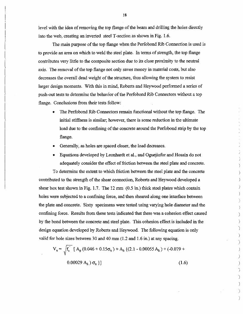
To determine the extent to which friction between the steel plate and the concrete
contributed to the strength of the shear connection, Roberts and Heywood developed a
shear box test shown in Fig. 1.7. The 12 mm (0.5 in.) thick steel plates which contain
holes were subjected to a confining force, and then sheared along one interface between
the plate and concrete. Sixty specimens were tested using varying hole diameter and the
confining force. Results from these tests indicated that there was a cohesion effect caused
by the bond between the concrete and steel plate. This cohesion effect is included in the
design equation developed by Roberts and Heywood. The following equation is only
valid for hole sizes between 30 and 40 mm (1.2 and 1.6 in.) at any spacing.
Yu= F [Ap(0.046+0.15cr0 )+Ah {(2.1-0.00055Ah)+(-0.079+
0.00029 Ah) cr0 } ] (1.6)
)
)
)
)
)
)
)
)
)
)

19
Fig. 1.6. Inverted steel T-section with perfobond rib shear connectors.
60mm
1-- .. 1
confining force
250mm
i...l •a---200 mm __ ..,.,!
Fig. 1.7. Roberts and Heywood's shearbox test.
:-i-50mm
t lOOmm
12mm
concrete block

Where:
20
Vu = Shear force per shear plane, N.
Ah = the hole area, mm.
Ap = the plate area in contact with the concrete less the hole area, mm.
crn = the stress normal to the plate, MPa.
f 'c = the concrete strength, MPa.
For determining the stress normal to the plate ( crn ), strain gages were placed on
the transverse reinforcement, and the average strain was measured. This average strain
was used to calculate the stress normal to the connector, which is in tum used in the
above equation to calculate failure loads.
In all applications, the shearbox equation slightly underestimated the failure load.
Thus, if the stress normal to the plate ( O'n ) is a known variable, then this equation appears
to be accurate. However, in the design of a given structure, this stress will not be known;
thus, the hole area (Ah) and the contact area (Ap) can not be determined using this
equation. Therefore, an equation is needed that can accurately determine the effect of
friction and cohesion based upon the dimensions of the steel plate and amount of
transverse reinforcement present.
In addition to push-out tests, a full-scale bridge was designed and constructed
with one section utilizing the inverted steel I-section with Perfobond holes. The bridge
was subjected to 500,000 cycles of loading equivalent to a T44 design truck plus impact
(AUSTROADS requirements). In addition, an ultimate load was applied to the slab to
investigate the transfer of load from the slab to the web of the T-section. There were no
measurable signs of deterioration during the fatigue testing, and no relative displacement
between the slab and T-section during the ultimate load test. Thus, the conclusion was
made that this type of design could be used as an economical alternative to existing
prestressed concrete designs.
)
)
)
)
)
)
)
)
)
)
)
)
)
)
)
)
)
21
2. SPECIMEN DETAILS
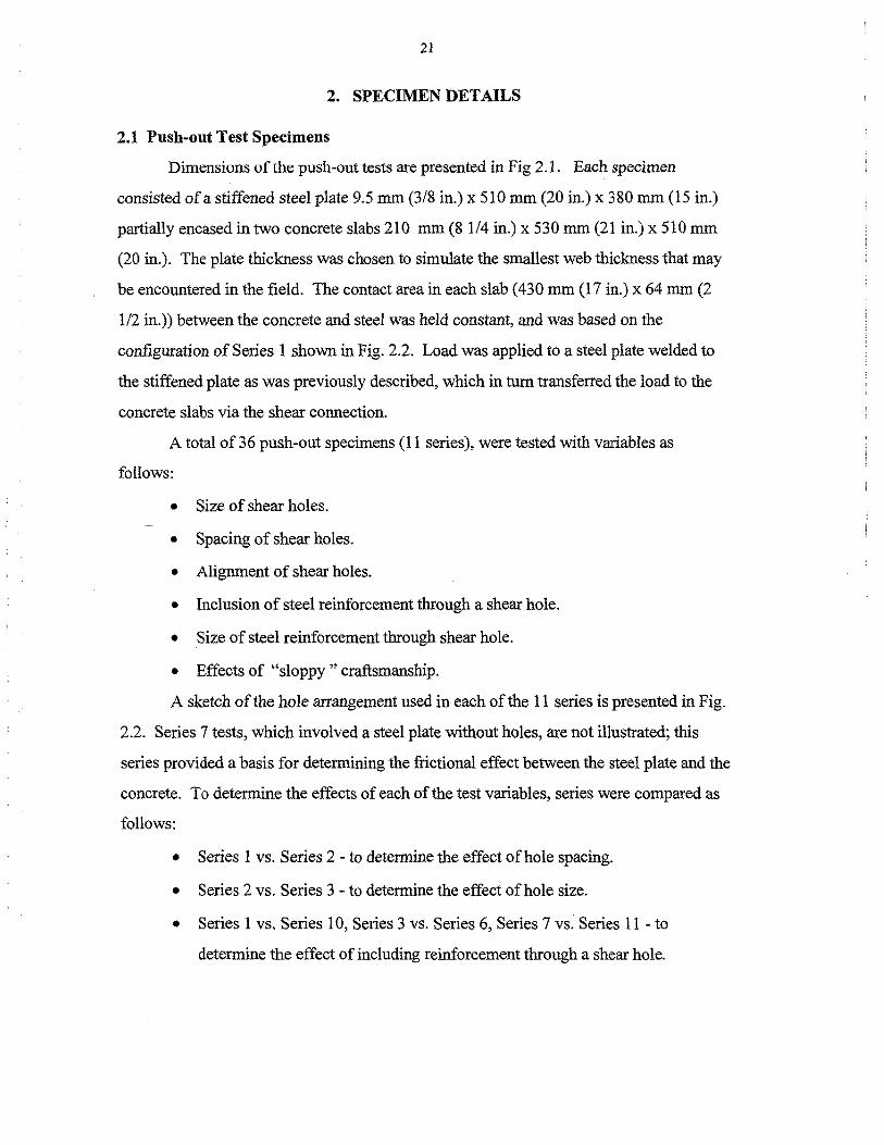
2.1 Push-out Test Specimens
Dimensions of the push-out tests are presented in Fig 2.1. Each specimen
consisted ofa stiffened steel plate 9.5 mm (3/8 in.) x 510 mm (20 in.) x 380 mm (15 in.)
partially encased in two concrete slabs 210 mm (8 114 in.) x 530 mm (21 in.) x 510 mm
(20 in.). The plate thickness was chosen to simulate the smallest web thickness that may
be encountered in the field. The contact area in each slab ( 430 mm (17 in.) x 64 mm (2
1/2 in.)) between the concrete and steel was held constant, and was based on the
configuration of Series 1 shown in Fig. 2.2. Load was applied to a steel plate welded to
the stiffened plate as was previously described, which in turn transferred the load to the
concrete slabs via the shear connection.
A total of36 push-out specimens (11 series), were tested with variables as
follows:
• Size of shear holes.
• Spacing of shear holes.
• Alignment of shear holes.
• Inclusion of steel reinforcement through a shear hole.
• Size of steel reinforcement through shear hole.
• Effects of "sloppy " craftsmanship.
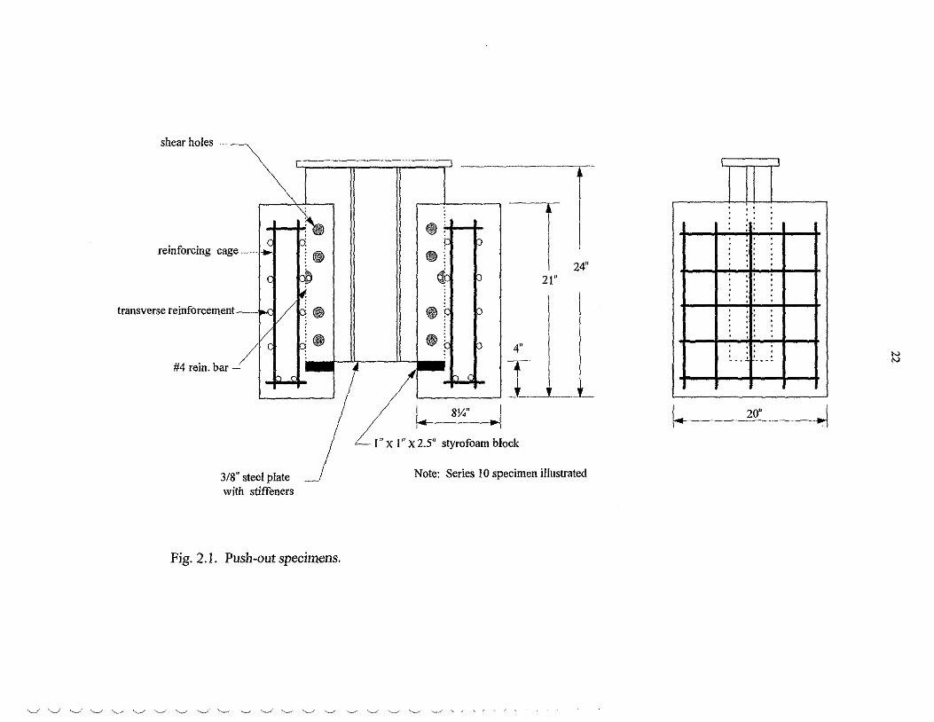
A sketch of the hole arrangement used in each of the 11 series is presented in Fig.
2.2. Series 7 tests, which involved a steel plate without holes, are not illustrated; this
series provided a basis for determining the frictional effect between the steel plate and the
concrete. To determine the effects of each of the test variables, series were compared as
follows:
• Series 1 vs. Series 2 - to determine the effect of hole spacing.
• Series 2 vs. Series 3 - to determine the effect of hole size.
• Series 1 vs. Series l 0, Series 3 vs. Series 6, Series 7 vs. Series 11 - to
determine the effect of including reinforcement through a shear hole.
shear holes -
reinforcing cage . •i
transverse reinforcement--
#4 rein. bar -
318" steel plate with stiffeners
Fig. 2.1. Push-out specimens.
f) ; I I
• •
--r 21"
4"
._____.I~. 1.. 8Y<" ~
-· - I" x I" X 2.5" styrofoam block
24"
Note: Series l 0 specimen illustrated
'._,• ,.._,- '-J .___, '......._/ --.__,, '....._,/ ~ '._.,f '--' .____. ,.._.,- ".._._/ -~ -.__,/ .._/ '--.,/ '---./ '---./ -~··-'
·1· .. . ' '' . ' ''
] ·1· '' '' '. '' ''
·1· '' . '. . ... - ....
(.. 20" ~
..., "'

2 1/2" ; I
t--"'"i
00000 17"
a. Series 1
00000
b. Series 2
4 1/2"
1• ... ;
00000
c. Series 3
#3 rein. bar \
~~-~,~--f'--~~
00 00
d. Series 4 #3 rein. bar \
\ ~_,,;-~
0 ° 0
e. Series 5
1 114" holes at 3" spacing
' + ! 112,,
1 1/4" holes at 2" spacing
3/4" holes at 2" spacing
1 1/4" holes at 3" spacing
1 1/4" holes at 3" spacing
23
3/4" holes at 2" spacing
#3 rein. bar ~ ~---3 ,..--+----,
00 00
f. Series 6
1 114" torched holes at 3" spacing
#4 rein. bar
0 0 0 0
g. Series 8
1 114" poorly torched holes at 3" spacing
#4 rein. bar
0 0 0 0
h. Series 9 1 1/4" holes at 3" spacing #4 rein. bar
0 0 0 0
i. Series 10
#4 rein. bar ~
I ~--
j. Seriesll
Fig. 2.2. Description of the hole arrangements used in the push-out tests.
24
• Series 4 vs. Series 5 - to determine the effect of shear hole alignment.
• Series 10 vs. Series 8 and Series 9 - to determine the effect of drilled holes vs.
torched holes and "sloppy" craftsmanship.
• Series 4 vs. Series 8 - to determine the effect of size of reinforcement through
the shear hole
Additionally, Series 7 and Series 11 were used to determine an expression to account for
the strength associated with excluding the shear holes. Data from all series were used in
the development of an expression for determining the shear strength of the ASC.
Transverse reinforcement in each of the concrete slabs was held constant for each
specimen, and was calculated based on recommendations presented by Leonhardt, et al.
[4]. The equation relating transverse reinforcement to reinforcement yield strength and
ultimate shear force is as follows:
A > .56Vu st -
fsy
Where:
(2.1)
Vu = Ultimate shear strength per hole, kN.
A,1 = Area of transverse steel required per hole, mm2•
f,y = Yield strength of the reinforcing steel, kPa.
The largest anticipated ultimate strength was used to determine that two #4 reinforcing
bars per shear hole were required for transverse reinforcement; this slab reinforcement is
shown in Fig. 2.1.
The first step in fabricating the push-out test specimens involved manufacturing
the shear holes in the 9 .5 mm (3/8 in.) steel plate. This was accomplished by either
drilling the holes with a magnetic drill or torching the holes. To fasten the lateral
stiffeners, 19 mm (3/4 in.) holes were drilled in the steel plate at the same time as the
shear holes. Voids were created in the concrete at the end of the steel plates by epoxying
styrofoam to the edge of the steel plates. This styrofoam was removed prior to testing to
create an unobstructed slip path for the steel plate (see Fig. 2.1 ).
)
)
)
)
)
)
)
25
To expedite the casting process, forms were fabricated so that three specimens
could be cast simultaneously. The steel plates were placed in the forms, followed by the
pre-fabricated reinforcing steel cages, being sure to restrict movement of the steel cages
in the forms. The concrete slabs were cast vertically so that both sides of the push-out
specimens could be poured at the same time, ensuring that the concrete strength would be
consistent in the slabs. A total of six specimens were cast per pour, using concrete from a
local ready-mix plant. The concrete was placed in three lifts and vibrated after each lift to
eliminate voids. Samples were taken throughout the casting to ensure slump and air were
within Iowa DOT standards, and to ensure that the concrete was consistent throughout the
pour.
In addition to the push-out specimens, fifteen 152 mm x 305 mm (6 in. x 12 in.)
standard ASTM concrete test cylinders and two 152 mm x 152 mm x 1,524 mm (6 in. x 6
in. x 5 ft) modulus of rupture beams were cast for each series. The push-out specimens,
cylinders, and beams were then covered with wet burlap and plastic and allowed to moist
cure for seven days. Formwork was removed after seven days and the specimens were
allowed to air cure until tested. All of the specimens were tested within two to three days
of the desired 28-day curing period.
2.2 BISB Laboratory Specimens
To obtain strength and behavior information on the original BISB, two specimens
which simulated a portion of the BISB were fabricated and tested in the laboratory. One
specimen had two steel beams and the other had four steel beams. Since the only
difference in the two specimens was the number of steel beams, only information
concerning the fabrication of the two beam specimen is presented in this report. In the
fabrication of the two-beam specimen, two 9,150 mm (30 ft) long l2W79 steel beams
were used, approximating the l2W77 beams used in most of the county BISB's. The
beams were positioned so the webs were 610 mm (2 ft) apart; steel straps (6.4 mm x 102
mm (l/4 in. x 4 in.)) were then welded at the third points to ensure the beams would
remain in position throughout the placing of the concrete.
Next, 1,220 mm (4 ft) plywood sections measuring 19 mm x 457 mm (3/4 in. x 18
in.) were placed on the bottom flanges of the two beams and glued to the steel using

26
PL400 structural adhesive. Approximately 63 mm (2 1/2 in.) gaps were left between the
web and the edge of the plywood so that concrete would be in contact with the bottom
flange (similar to that shown in Fig. 1.1 b ). Plywood sections were also used for the ends
of the specimens. These sections were bolted to the beams using fasteners that had been
previously welded to the steel beams. Like the original BISB, no reinforcing steel was
included in the structure. Lastly, all joints were sealed with caulk and allowed to cure
before concrete was poured.
A standard Iowa DOT bridge mix was obtained from a local ready-mix plant. The
concrete was placed in two lifts of approximately 152 mm (6 in.); the concrete.was
vibrated after each lift to ensure contact with the steel. Extra concrete was screeded off
and the exposed concrete troweled to create a smooth, level surface for the strain gages
that were added. Six 152 mm x 305 mm (6 in. x 12 in.) concrete test cylinders and one
152 mm x 152 mm x 1524 mm (6 in. x 6 in. x 5 ft) modulus of rupture beam were also
made.
The four-beam BISB specimen is illustrated in Fig. 2.3. As previously noted, the
same procedure was used in the fabrication of this specimen; the only difference between
the two is the additional beams (i.e., four beams rather than two beams).
2.3 Composite Beam Specimens
2.3.l Inverted T-Beam
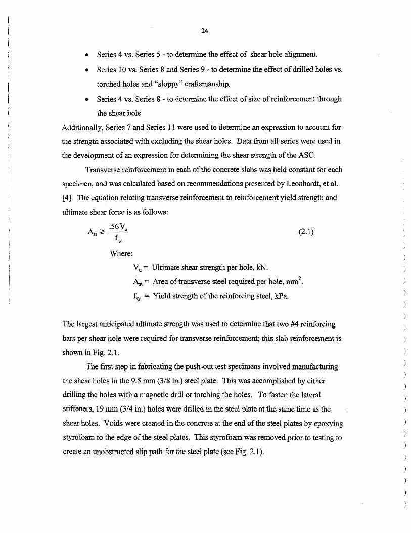
Specimen 1, illustrated in Fig. 2.4, consisted of a W2lx62 with its top flange and
25 mm (1 in.) of the web removed, giving it a depth of 492 mm (1 ft - 7 3/8 in.).
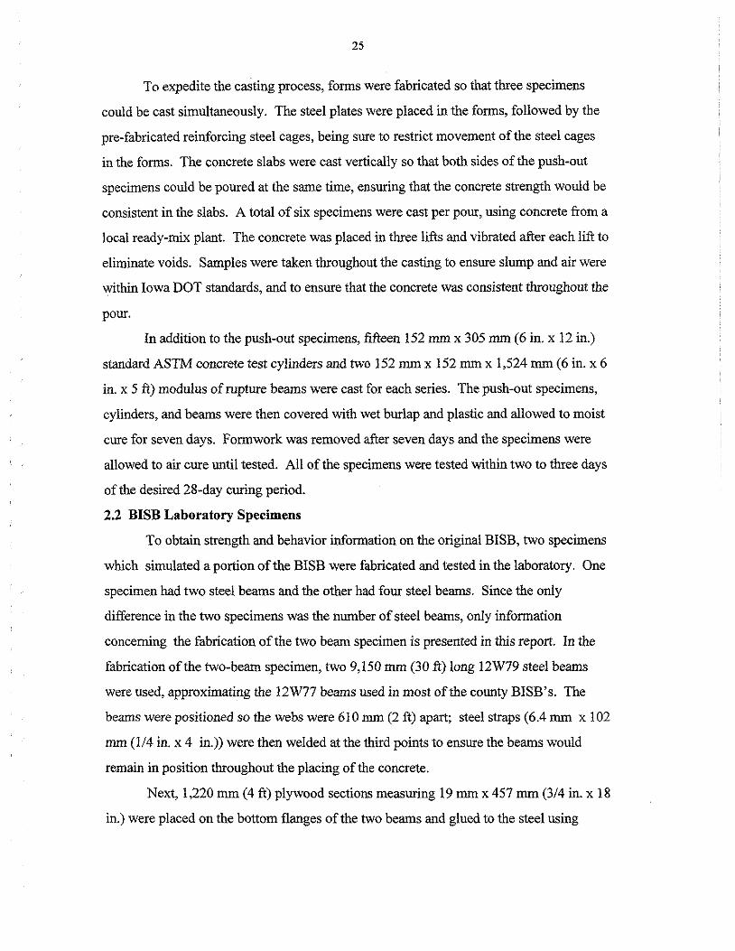
Information on cutting off the top flange is given at the end of this section. Holes 27 mm
(1 1/16 in.) in diameter on 102 mm (4 in.) centers and 457 mm (18 in.) from the top of the
bottom flange were drilled in the web (see Fig. 2.4c). A 152 mm (6 in.) deep slab, 610
mm (24 in.) wide, was poured to form a specimen with a total depth of 584 mm (23 in.).
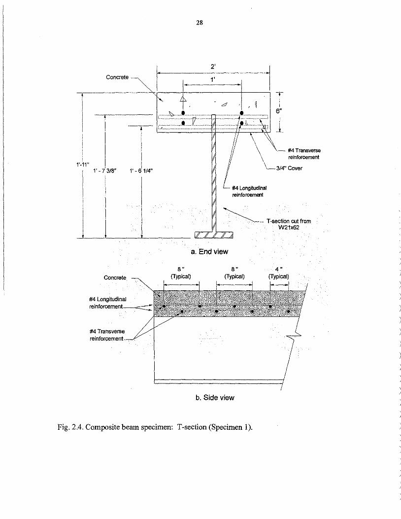
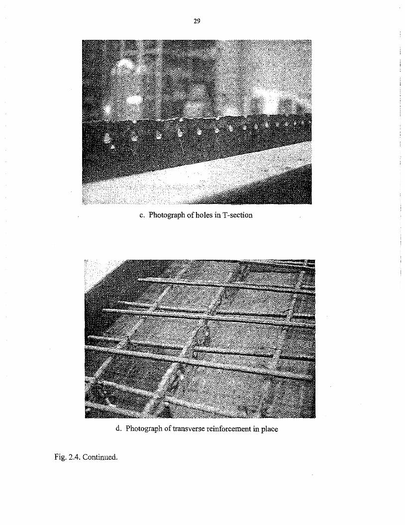
Reinforcement was placed in every other hole. A second layer of reinforcement was
placed in 13 mm (1/2 in.) grooves cut at the top of the T-section (see Fig. 2.4d). The
second layer ofreinforcement offset from the first layer by 102 mm ( 4 in.) was placed on
203 mm (8 in.) centers. A layer oflongitudinal reinforcement was placed on top of the
transverse reinforcement. This reinforcement consisted of two #4 reinforcing bars spaced
)
)
)
)
)
)
)
)
)
)
)
)
)
)
)
)

27
24" 24" 24"
C te ' oncre _
7 ' ' W12x79~ ! I I I
JI ' ' ' <l ' "' . <l ' "' <l ' "' () () ()
' ' ' " ~ "" " ~ "" " ~ "" " ' " ' " '
18" .I 3/4"Plywo~ .. (Typical)
a. End view
b. Photograph of BISB four-beam specimen
Fig. 2.3. Cross section ofBISB four-beam specimen.
1'-11"
Concrete
1' -7 3/8"
Concrete
l I
1'-~1/4"
#4 Longitudinal reinforcement--=:::::::
#4 Transverse reinforcement
8" (Typical)
28
2'
·1 1'
J , ~
#4 Longitudinal reinforcement
J I
-L
#4 Transverse reinforcement
314" Cover
~- T-section cut from W21x62
a. End view
8" 4" (Typical) (Typical)
b. Side view
Fig. 2.4. Composite beam specimen: T-section (Specimen 1).
' )
29
c. Photograph of holes in T-section
d. Photograph of transverse reinforcement in place
Fig. 2.4. Continued.

30
152 mm (6 in.) from the center of the T-section. During placement of the concrete, the
formwork was fully supported. The formwork was then removed when the concrete
reached a compressive strength of 10. 7 MPa (3,000 psi).
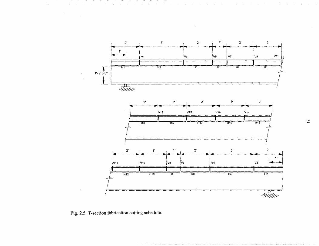
The T-section used in this specimen was fabricated by cutting off the top flange
and 25 mm (1 in.) of the web of a 10,360 mm (34 ft) Jong W21x62. To minimize
possible out of plane bending, the beam was cut while supported on its bottom flange. In
this position, it was simply supported on a clear span of9,750 mm (32 ft).
Due to safety concerns, it was decided that the beam would be cut in horizontal sections,
each 305 mm to 915 mm (1 ft to 3 ft) long, with consecutive cuts alternating between
each end of the beam. The cuts were made using an acetylene/oxygen torch. Each cut
consisted of a horizontal cut through the web at a distance of 19 mm (3/4 in.) from the
bottom of the top flange. Following this cut, a vertical cut through the flange was made
separating the top flange from the original beam. The first two cuts were not followed by
a vertical cut; only after the third and fourth cuts were vertical cuts made separating these
pieces from the rest of the specimen. A total of 17 horizontal and 15 vertical cuts were
made, as shown in Fig. 2.5. To simulate the worst case scenario for cutting the top flange
of the specimen, an inexperienced individual was used to cut the specimen.
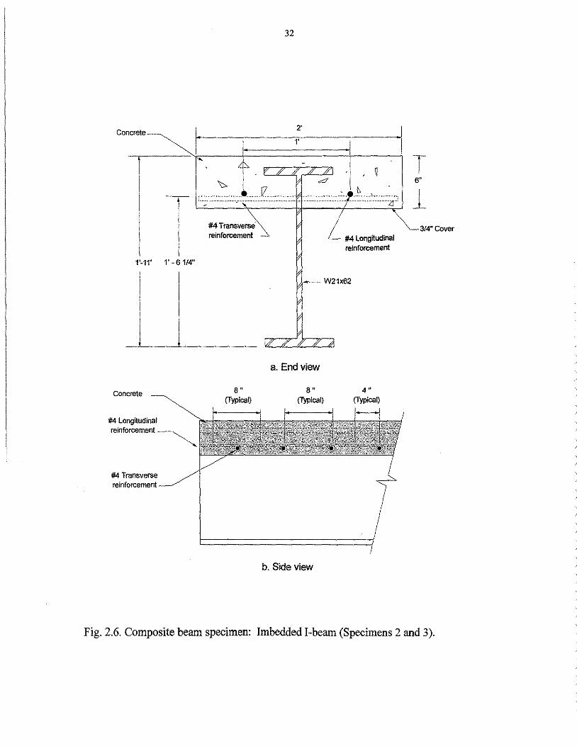
2.3.2 Imbedded I-Beam
Specimens 2 and 3, shown in Fig. 2.6, consisted ofW2lx62's with the top flange
imbedded in a concrete slab. Like Specimen 1, the concrete slab was 610 mm (24 in.)
wide and 152 mm (6 in.) in depth. Holes 27 mm (l 1/16 in.) in diameter were drilled 457
mm (18 in.) above the top of the bottom flange on 102 mm (4 in.) centers. For transverse
reinforcement, #4 reinforcing bars were placed in every other hole. The slab was
positioned so that the top flange of the imbedded beam had 51 mm (2 in.) of concrete
cover. The total depth of the entire section was 584 mm (23 in.). Two speciniens were
constructed due to testing problems with Specimen 2; these problems are discussed in Ch.
5 where a comparison of results from the two specimens (Specimens 2 and 3) is
presented.
)
)
)
)
)
)
1. 2' ""'·,---------3-· ----t3 ___ 2' --r~t7 ___ 2· 1. 2'
V111
I I I I I f
1'-7 3~8" !,,._
Hl ~ H5 H7 H9 ;11
_L l==::;::;::===============t "
2' 2' 2' 2' 2'
I· .. I. + .. 1----+- .J V13 V15 V16 V14
H13 H15 H17 H16 H14
I .. 2' ·t-2._tT2
• _1_ 3'
21~ -1~ V2
H12 H10 H8 H6 H4 H2
·~
Fig. 2.5. T-section fabrication cutting schedule.
w -
Concrete
-.-1
1'-11' 1' -61/4"
Concrete
#4 Longitudinal reinforcement~
#4 Transverse reinforcement
#4 Transverse· reinforcement
8" (Typical)
32
2'
1'
#4 Longitudinal reinforcement
-W21x62
a. End view
8" (Typical)
b. Side view
4" (Typical)
T 6"
1 3/4" Cover
Fig. 2.6. Composite beam specimen: Imbedded I-beam (Specimens 2 and 3).
)
)
)
)
)
)
)
)
)
)
)
)
33
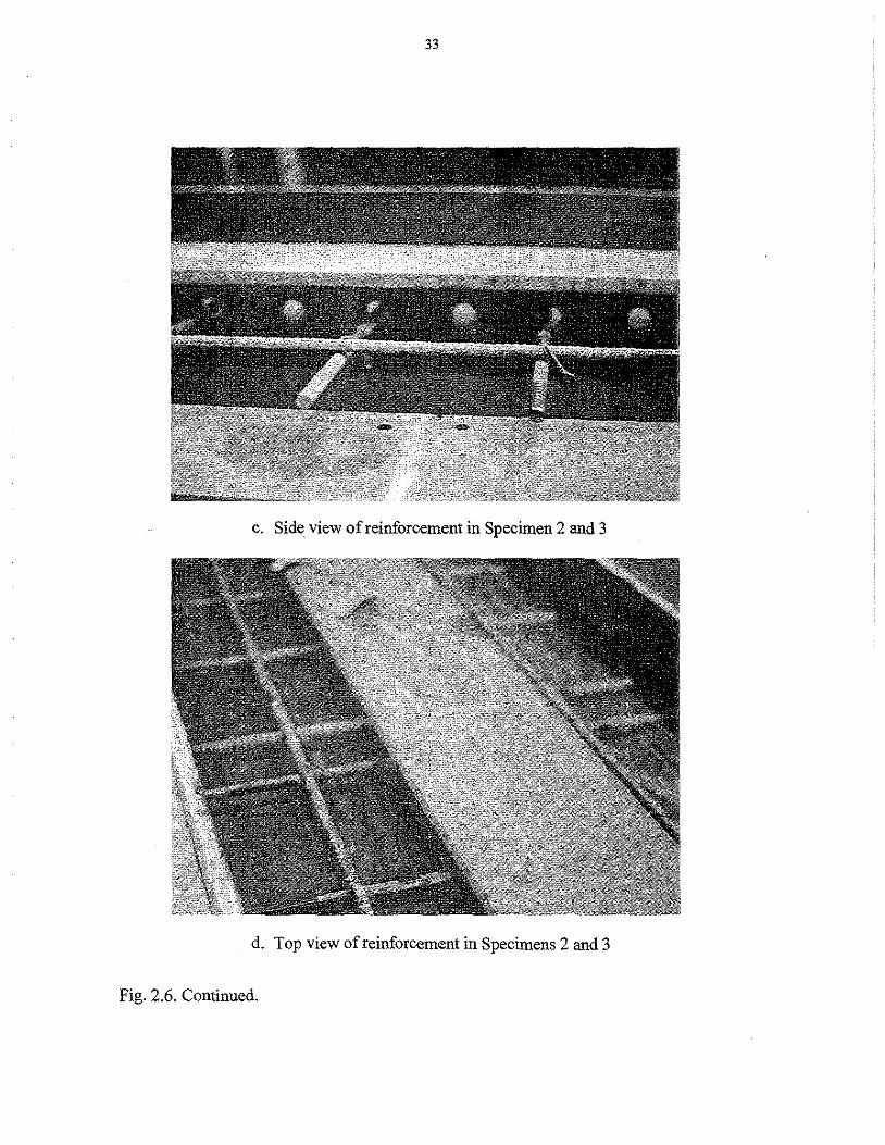
c. Side, view of reinforcement in Specimen 2 and 3
d. Top view of reinforcement in Specimens 2 and 3
Fig. 2.6. Continued.

34
2.3.3 Standard Composite Beam
Specimen4, shown in Fig. 2.7, consisted ofa W21x62 with a 610 mm (24 in.)
wide, 152 mm (6 in.) deep slab. Standard 102 mm (4 in.) shear studs, 13 mm (1/2 in.) in
diameter, were placed on 305 mm(! ft) centers along the entire length of the specimen,
based on the ultimate load criteria in AASHTO Bridge Design Specification (13).
Reinforcement in the slab consisted of two layers of #4 reinforcing bars. The first
layer was placed 25 mm (1 in.) above the top flange of the concrete and spaced every 203
mm (8 in.). The second layer ofreinforcement was placed 102 mm (4 in.) above the top
flange, also on 203 mm (8 in.) centers. Longitudinal reinforcement, consisting of#4 bars,
was placed 152 mm (6 in.) from the center of the cross section (see Fig. 2.7c). The
longitudinal reinforcement was placed directly upon the transverse reinforcement along
the entire length of the span; thus, the longitudinal reinforcement layers were 38 mm (1
1/2 in.) and 114 mm ( 4 112 in.) above the top flange.
2.4 BISB Field Bridge
A representative BISB in Benton County was service lo.;id tested to obtain
strength, deflection, and strain data. The road leading to the bridge was noted as a Level
B service gravel road, often subject to flooding. Complete drawings and dimensions for
the bridge are presented in Fig. 2.8 and Tables 2.1 and 2.2. Beams were typically spaced
at 610 mm (24 in.), with bearings of520 mm (20 1/2 in.) and 305 mm (12 in.) on the east
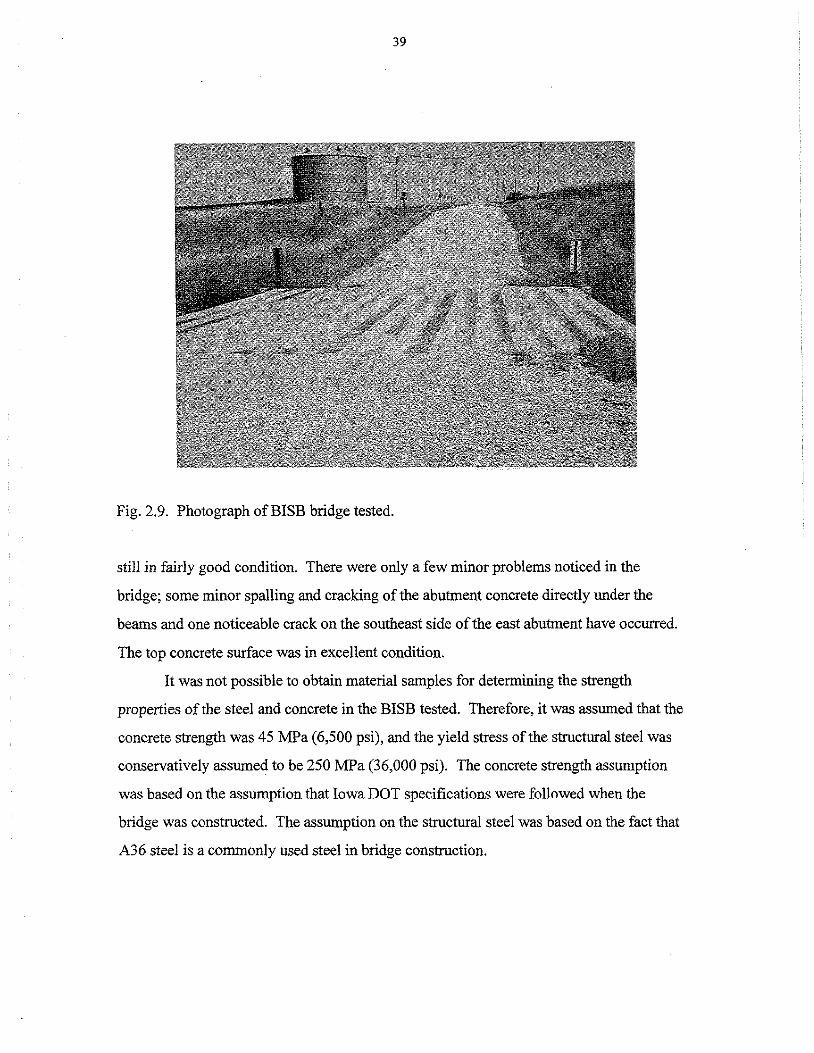
and west ends, respectively. A photograph of the bridge tested is shown in Fig. 2.9.
Construction drawings indicated the bridge superstructure was attached to the
abutment by 2 #8 reinforcing rods at each end, which extended into the bridge 152 mm
(6 in.) (see Fig. 1.3). This reinforcement provided a certain rotational fixity at the end
supports. The abutment, shown previously in Fig. 1.2, consisted of 9 steel piles on 1,220
mm ( 4 ft) centers in the abutment face, with wingwalls constructed to the desired height.
Reinforcement on 305 mm (12 in.) centers was spaced around the outside of the entire
abutment and wing walls.
Overall, the bridge was in very good condition. There was evidence of frequent
flooding of the stream, causing minor corrosion problems on the lower flanges of the
beams, and some erosion in the vicinity of the abutments. The plywood formwork was
)
)
)
)
)
)

35
2'
concrete 1'
i 2'-5" 2'-3 1/2" 2'-1/2"
Concrete
#4 Transverse reinforcement
4" Shear stud 1/2 ° diameter
a. Front view
#4 Longltudinal reinforcement
W21x62
8" (Typical)
8" (Typical)
4" (Typical)
b. Side view
Fig. 2.7. Composite beam specimen: Welded studs (Specimen 4).
#4 Transverse reinforcement
1" Cover
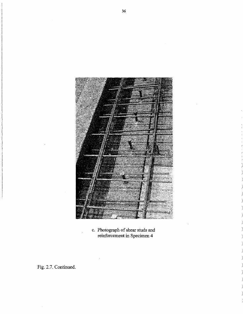
Fig. 2.7. Continued.
36
c. Photograph of shear studs and reinforcement in Specimen 4
)
)
)
)
)
)
)
)
)
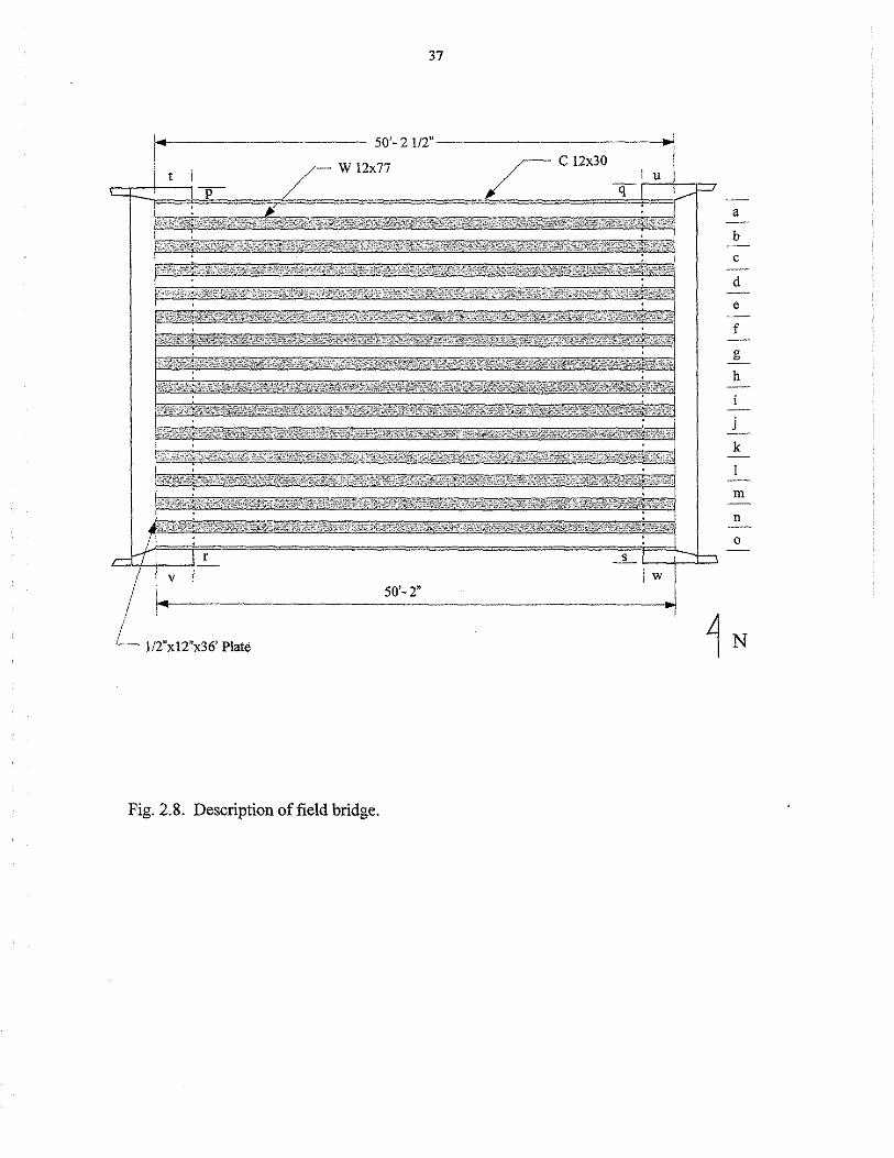
37
I t /- C12x30
I u•1 -q I
------------ 50'-2 l/2"-------------
/- W 12x77 I p
I
: I
; I
. I
. I
I
I
I
I I
I -r7 I r _s_ I'---+--'--'
I v I 50
,_ 2
,, l w
~,~~~~~~~~~~~~~~~~~~-o.i
L J/2"x!2"x36' Plate
Fig. 2.8. Description of field bridge.
a
b
c
d
e
f
g
h
j
k
m
n
0

38
Table 2.1. Beam spacing in field bridge.
Beam Spacing West Side East Side (in.) (in.)
a 24 1/8 24112
b 23 15/16 24 1/16
c 24 1/16 23 3/4
d 24 24118
e 24 1/8 24 1/8
f 23 5/8 24 3/16
g 24 1/4 24
h 243/8 24 3/8
1 24 1/8 . 24
j 24 3/8 23 5/8
k . 24 3/16 24114
I 23 5/8 23 5/8
m 24 24 3/16
n 24 23 11116
0 241/4 24 1/8
Table 2.2. Field bridge abutment measurements.
Abutment Measurement Dimension (in.)
p 461/2
q 35
r 37
s 46
t II 7/8
u 20 3/8
v 12 1/2
w 20 3/8
)
)
)
)
)
) \ )
39
Fig. 2.9. Photograph ofBISB bridge tested.
still in fairly good condition. There were only a few minor problems noticed in the
bridge; some minor spalling and cracking of the abutment concrete directly under the
beams and one noticeable crack on the southeast side of the east abutment have occurred.
The top concrete surface was in excellent condition.
It was not possible to obtain material samples for determining the strength
properties of the steel and concrete in the BISB tested. Therefore, it was assumed that the
concrete strength was 45 MPa (6,500 psi), and the yield stress of the structural steel was
conservatively assumed to be 250 MPa (36,000 psi). The concrete strength assumption
was based on the assumption that Iowa DOT specifications were followed when the
bridge was constructed. The assumption on the structural steel was based on the fact that
A36 steel is a commonly used steel in bridge construction.

41
3. TESTING PROGRAM
The experimental portion of the investigation consisted of several different
laboratory tests plus one field test. Details of these tests as well as the instrumentation
used are presented in this chapter.
Instrumentation for the various tests included three different measuring devices.
For measuring displacements (slip, deflection, and rotation), either direct current
displacement transducers (DCDT's) or Celesco string potentiometers (Celescos) were
used. Strain data were obtained using electrical-resistance strain gages (strain gages).
The strain gages were attached to the base material (steel or concrete) using
recommended surface preparations and adhesives. All strain gages were water proofed
and covered to prevent moisture or mechanical damage. Lead wires were connected to
the gages using a thi:ee-wire hook-up to minimize the effect of the long lead wires and
temperature changes.
After installing the instrumentation, the lead wires were then connected to a
computer controlled data acquisition system (DAS). With the DAS, deflections from the
Celescos and DCDT' s, as well as strains from the strain gages, can be measured and
recorded. All pertinent data were automatically stored on the computer hard drive, where
it was later accessed and copied onto a computer disk.
3.1 Push-out Tests
Slip and separation between the concrete slabs and the steel plate data were
acquired on all push-out specimens (see Fig. 3.1). All 36 specimens were instrumented in
the same manner, using seven DCDT's. Two of the DCDT's were fastened rigidly to the
plate stiffeners for measuring slip between the concrete slabs and steel plate. The stems
of the DCDT' s were attached to wooden blocks that had been epoxied to the concrete
slabs. Thus, the slip was measured relative to the centerline of the shear connectors.
Four of the DCDT's, used to measure separation between the concrete slabs and
the steel shear plate, were rigidly attached to the base of the universal testing machine.
Separation was measured at the top third point, and 76 mm (3 in.) below the bottom third
point. It was assumed that if separation occurred, it would take place near the bottom of
the slab; thus, the reason for placing the DCDT' s lower than the bottom third point.

T 14"
Ci
•@ 9
.@
@)
42
~ DCDTm-;"''"'" a. Top view of-plane bending
b. Side view
@
@.
41
~· """ . ""'•
-DCDT1s measuring concrete block movement
DCDT's measuring relative slip
Fig. 3.1. Location of instrumentation used in the push-out tests.
)
\ )
)

43
The remaining DCDT was used to measure lateral deflection of the stiffened
plate. It was initially a concern that large loads on the 9.5 mm (3/8 in.) thick steel shear
plate might induce lateral buckling. Stiffeners were placed on the steel shear plate to
prevent such buckling. The DCDT was used to monitor lateral displacements (i.e., out of
plane bending).
To obtain uniform load distribution, 6.5 mm (1/4 in.) neoprene pads were placed
under each of the concrete slabs. Load was applied to the top edge of the steel plate by
the head of the testing machine through a 13 mm (112 in.) thick steel distribution plate,
tack welded to the top of the steel shear plate. Care was taken prior to testing to level the
top edge of the steel shear plate, which in turn ensured the welded distribution plate was
level. Additionally, before loading, the position of each specimen was checked carefully
to ensure it was "centered" in the testing machine so that load would be distributed
equally to the two slabs.
Testing began with an initial load of approximately 1.8 kN (400 lbs). The initial
load was applied to make sure the deflection and slip instrumentation was operating
correctly, and to ensure an even distribution of force through the distribution plate on the
edge of the steel shear plate.
It has been reported by Slutter and Driscoll ( 11) that shrinkage of the concrete is
sufficient enough to destroy the bond between the concrete and the steel shear plate. By
destroying this bond, the entire load will be carried by the connection, thus inducing
consistent and duplicable results (Siess, Newmark, Viest, (14)). In addition, in 1970,
Ollgard (15) noted that the load-slip curve would not be affected by unloading and
reloading the specimen. According to this, the initial load would not affect the final
results.
3.2 BISB Laboratory Tests
3.2.1 Two-Beam Specimen
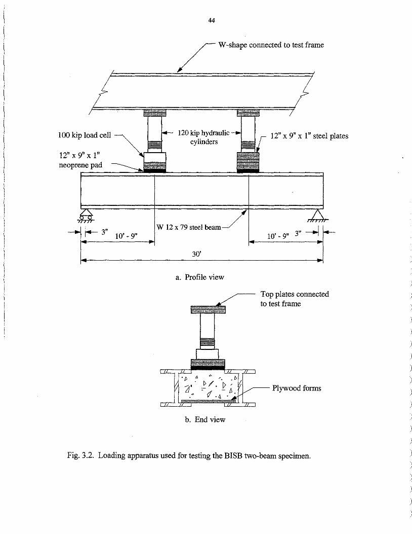
Using a test frame which was anchored to the structures laboratory floor, the load
was applied to the composite beam specimen through two 534 kN (120 kip) hydraulic
cylinders. The two-point loading system was used to create a constant moment region in
the specimen. As shown in Fig. 3.2a, the loading points were located 3,300 mm (10.75
100 kip load cell
12" x 9" x 1" neoprene pad
44
/ W-shape connected to test frame
J 20 kip hydraulic cylinders
W 12 x 79 steel beam_/
30'
a. Profile view
b. End view
12" x 9" x 1" steel plates
Top plates connected to test frame
Fig. 3.2. Loading apparatus used for testing the BISB two-beam specimen.
)
)
)
)
)
)
)
)
)
45
ft) from the center line of the end supports, which provided a constant moment region of
2,440 mm (8 ft).
As in the push-out tests, neoprene pads were placed between the loading
distribution plates and the concrete to transmit force uniformly to the concrete. The load
was applied directly on the 305 mm (12 in.) concrete of the composite beam, between the
two steel beams (see Fig. 3.2b). One 445 kN (100 kip) load cell placed under the left
hydraulic cylinder was used to determine the load on the structure. Since one pump was
used for both hydraulic cylinders, it can be assumed that the two hydraulic cylinders
applied the same force. Magnitudes of applied load were recorded by the DAS, and were
saved along with all other pertinent strain and deflection data.
Strain gages and Celescos were installed on the steel beam prior to the pouring of
the concrete to determine the amount of strain and deflection that occurred during placing
of the concrete. DCDT' s were later installed at the supports to measure the slip between
the steel beams and the concrete. Location of strain gages, Celescos, and DCDT' s used
in the tests are shown in Fig. 3 .3. Strain gages were used to measure strains on the top,
mid-height, and bottom of the steel beams, at 1/4, 112, and 3/4 of the span. The Celescos
were used to measure deflections at the same three locations. At Sections 1 and 2, the
Celescos were mounted on the bottom of each of the steel beams, as well as on the middle
of the plywood. At Section 3, one Celesco was mounted in the middle of the plywood to
check for symmetry along the span. A total of 18 strain gages, 4 DCDT' s, and 7 Celescos
were used in testing the composite beam.
Two load tests were performed on the composite beam. In the first test, the load
was applied in 2.22 kN (500 lbs) increments. After each load increment, strains,
deflections, and slip measurements were taken and recorded using the DAS. The
composite beam was loaded past yielding of the steel, to the 445 kN (100 kip) capacity of
the load cell. Thus, a total load of 890 kN (200 kip) was applied to the specimen. The
composite beam was then allowed to sit overnight to "relax." Measurements were taken
throughout the night to determine the rate and extent to which the composite beam
recovered. The following day, another load test was performed in the same manner to
determine the reserve capacity of the composite specimen.

46
' ' ' i
=- " ' -' '
~ L.: :....J L::;::_J '
I 111 ' ' r- 3"
7'-7.5" 7'- 4.5" 7'- 4.5"
30'
Symbols:
=-i = DCDTs
• = Strain gages
c::::J = Celescos
Fig. 3.3. Instrumentation for the two-beam specimen.
"
L.; :...J
-=
~ 3" -.j ~
7'- 7.5"
)
)
)
)
)
)
)
)
)
)
)
)
)
47
3.2.2 Four - Beam Specimen
To determine the response of the bridge during load testing, the specimen was
instrumented with 40 strain gages and 11 Celescos. The strain gages were placed at three
different sections along the span: the quarter point, the centerline, and three quarter point,
as shown in Fig. 3.4. Strain gages located on steel beams were placed at the center of the
top surface of the top flange, at mid-height of the web, and at the center of the bottom
surface of the bottom flange. Concrete strain gages were placed on the top concrete
surface midway between the steel beams. The primary purpose for installing strain gages
at the three quarter point was to check for symmetry about the centerline of the specimen.
The location of the three instrumented cross sections is shown in Fig. 3 .5.
Figure 3 .5 also shows the location of the Celescos that were used to measure
deflections. The Celescos are located on each beam at the quarterpoint, three-eighths
point, centerline, and three-quarter point. The two Celescos at the three-quarter point
were for determining ifthe specimen was responding symmetrically about its centerline.
Testing of the four-beam specimen was different from the testing of the two-beam
specimen, in that a single service load was applied at several locations so that the lateral
load distribution in the system could be determined. The single point load had a surface
contact area of305 mm x 305 mm (1 ft x 1 ft). To insure that the specimen was not over
stressed during the service level load tests, a maximum magnitude of 89 kN (20 kips) was
used for the single point load. Calculations made prior to testing indicated that by
limiting the applied load to this magnitude, stresses in the specimen would remain in the
elastic range. As shown in Fig. 3.6, the load was positioned at the center of each steel
beam or concrete section at distances of 1,500 mm, 2,720 mm, 3,940 mm, and 4,750 mm
(4 ft- 11 in., 8 ft- 11in.,12 ft- 11 in., and 15 ft- 7 in.) from the centerline of the pin
support. As shown in this figure, load was applied at 25 different locations; for purposes
of discussion, applying load at a given location is referred to as a "test." Thus, there were
25 service load tests. Each test is identified by an (x,y) notation which indicates the
position of the load on the specimen. The x notation varies from A to G and indicates
where the loading is located transversely; the y notation varies from 1 to 4 and indicates

48
1' 1' 1' 1' 1'
' ' <\ ' "". <\ ' "" <\ ' "" 0 0
i ' ' '
0 l LI 0 l LI 0 ~
6" A 4
A 4
A
l
a. Section at 1/4 span
~in gage locations
' ' <\ ' "" <\ ' ""
<\ ' "". 0 0
' - ' 0 l 6 0 l 6 0
~ . ' 0 4
A
b. Section at midspan
' ' <\ ' "" <\ ' ""
<\ ' "" 0 0 ' - ' -
0 l LI 0 l LI 0
~ A ' A 4
A
c. Section at 314 span
Fig. 3 .4. Location of strain gages on four-beam specimen.
1'
'
0 6
4
' 0
LI 4
'
0 6
4
'
'
'
• J
)
)
)
)
)
)
)
)
)
)
)
)
)
)
)
)
)
)
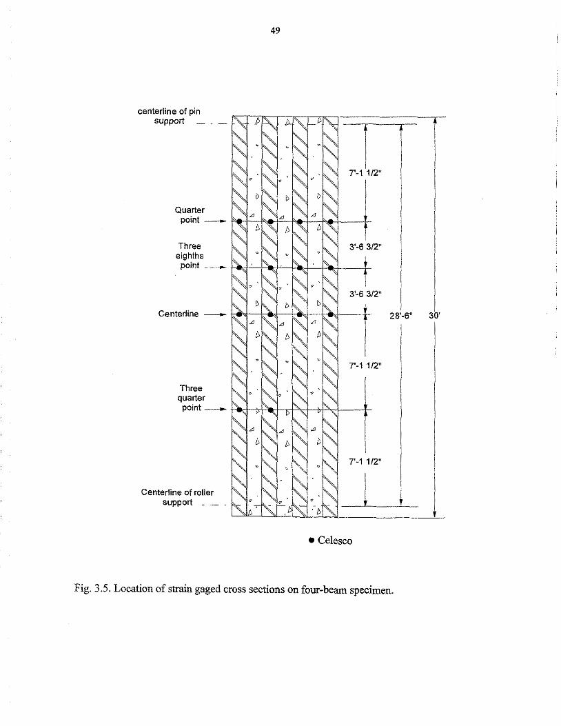
centerline of pin support _ . _
Quarter
49
point - f\e-1---cf'~=-
Three eighths
I 7'-1 1/2"
point - ~d--t"1"---t-ll~'--t~t--+
Three quarter
7'-1 1/2"
point - ~+-t+"1,--,;f-"cl--+t""t--+
Centerline of roller support • _ .
7'~1 1/2"
• Celesco
28'-6" 30'
I
j
Fig. 3.5. Location of strain gaged cross sections on four-beam specimen.

Section F Section E Section D Section C Section B Section A
Centerline of pin support
Neoprene
pad~
50
4' 3'-8"
. '
i Section
1 Section
2 Section Section
3 4
a. Plan view
~~-~--- Hydraulic cylinder Load cell
~Steel plate
' .
b. Cross section
' .
•Load point
Connected to loading frame
' .
i Centerline of roller support
Fig. 3.6. Location of loading points for service level load testing the four-beam specimen.
)
)
)
51
the longitudinal location of the load. For example, Test Al refers to the load being placed
on the exterior steel beam at a distance of 1,500 mm (4 ft - 11 in.) from the pin support.
Similarly, Test D3 refers to the load being placed on the center concrete section at a
distance of3,940 mm (12ft- 11 in.) from the pin support. The location of these load
points and corresponding sections are shown in Fig. 3.6.
The loading setup shown in Fig. 3.7 consisted of a neoprene pad, 305 mm x 305
mm x 25 mm (1 ft x l ft x 1 in.), placed on top of the specimen. Placed directly on top of
the neoprene pad were 25 mm ( 1 in.) thick steel plates with the same dimensions as those
of the neoprene pad. The purpose of these steel plates was to provide a uniform
distribution of load to the specimen and to reduce the space between the loading frame
and the specimen. The applied load was measured by a load cell, which was placed on
top of the steel plates. A steel spacer plate was positioned on top of the load cell to insure
that the load was applied to the center of the load cell; this is required for correct
measurement of loads. A hydraulic cylinder, with a maximum load capacity of 534 kN
(120 kips) and a stroke limit of 152 mm (6 in.) was used to apply the load. As shown in
Fig. 3. 7, four point loads were used in the ultimate load test. Load were applied through
holes formed in concrete in the specimen when it was cast. The holes were located 2,970
mm (9 ft - 9 in.) from the center of the supports in the center of the concrete sections. A
Dywidag bar was position in the precast holes in the specimen and connected to the tie
down floor. With the hydraulic cylinder positioned as shown, load could be applied to the
specimen.
Deflection and strain readings were taken using the same program and DAS used
in the service load tests. Because all four hydraulic cylinders were connected in parallel
to the same hydraulic pump, it was necessary to monitor the applied load at only one load
point. Strains, deflections, and loads were measured and recorded using the DAS after
every 2.22 kN (500 lbs) increment ofload.
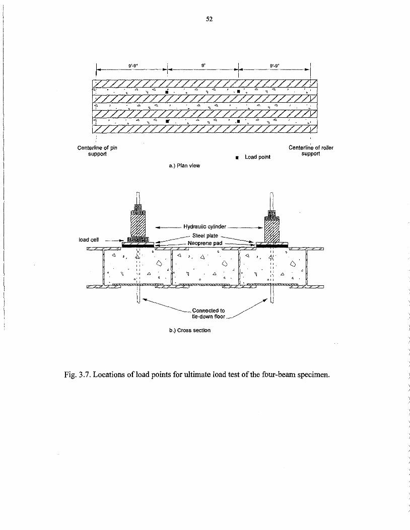
Centerline of pin support
load cell
<\
1
52
• Load point a.) Plan view
n
...,__ ___ Hydraulic cylinder ____ ...
~Steel plate Neoprene pa~
v " ~- <\ ,, <I <\ ~:· () () "
" " "' 1 "' 1 ,., o" ' ' 0" "
~Connected to / tie--down floor~
b.) Cross section
"'
Centerli~e of roller support
()
'
Fig, 3. 7. Locations ofload points for ultimate load test of the four-beam specimen,
)
)

53
3.3 Composite Beam Tests
strain gages were placed at the quarter point, centerline, and three-quarter point of
the specimens. The same sections in each specimen were instrumented; however, the
location of the strain gages at each section varied from specimen to specimen, as is shown
in Fig. 3.8. The instrumentation for measuring the deflections was the same for each
specimen. Seven Celescos were placed along the length of the span and were positioned
as shown in Fig. 3.9. Two DCDT's were placed at each end of the beam to measure the
slip between the concrete slab and steel beam.
3.3.1 Service Load Tests
The total length of each specimen was 10,360 mm (34 ft), and the clear span was
9,750 mm (32 ft). Each specimen was tested as a simply supported beam.
Prior to testing, an initial calculation determined that yielding of the specimen would
occur when a load of 133 kN (30 kips) was applied. To insure that the specimen stayed
in the elastic range, a maximum load of 89 kN (20 kips), 66% of the load required for
yielding, was used during the service tests. As shown in Fig. 3.10, load was applied at
two points, each 610 mm (2 ft) from the center of the specimen. The applied load was
transferred through a steel plate to a 305 mm x 305 mm (1 ft x 1 ft) neoprene pad.
Loading was applied using hydraulic cylinders connected to the same pump. Thus, only
one load cell was required to measure the applied force. There were three service load
tests for each specimen to check the reproducibility of the response. The service tests
consisted of loading each specimen to a maximum total load of 89 kN (20 kips) in
increments of2.22 kN (500 lbs). As with previous tests, strains and deflections were
measured and recorded using the DAS after each load increment.
3.3.2 Ultimate Load Tests
After completion of the service load tests, each specimen was loaded to failure.
The failure tests were setup the same as the service test with two load points placed 1,220
mm (4 ft) apart (see Fig. 3.10). As during the service load tests, the strains and
deflections were measured after each 2.22 kN ( 500 lbs) load increment. In each test, the
stroke limit of the cylinder was reached before failure of the specimen occurred. At this
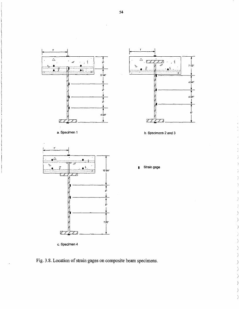
1' ·I 6
d
a. Specimen 1
I· 1'
c. Specimen 4
, ~ I 5'
t 51/4"
j J I
4 314tt
1..
I ,L l
54
I· 1' ·I 6
\, d
'
b. Specimens 2 and 3
1 Strain gage
Fig. 3.8. Location of strain gages on composite beam specimens.
,L J
4 314"
j
43/4"
I 5'
)
)
)
)
)
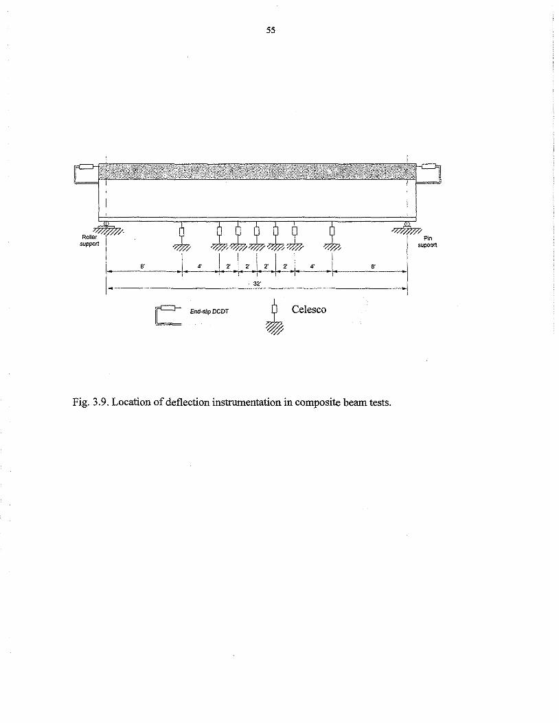
Roller support
8'
'/
I •. ' "'
L En~slipDCDT
55
4' 8' I
Celesco
Fig. 3.9. Location of deflection instrumentation in composite beam tests.
'/ Pin
supoort

11 I
Centerline of pin support
Load cell-
'tZ-3"
4'
56
4'
• Load point
a.) Plan view
.,.__ __ Hydraulic cylinder ___ _,._
--------- Steel plate(s) -------Neoprene pad
. "" . ,_ 4'
b.) Side view
Fig. 3.10. Composite beam test setup.
Centerline of roller support
"" .
J
)
)
)
)
)
)
)
)
)
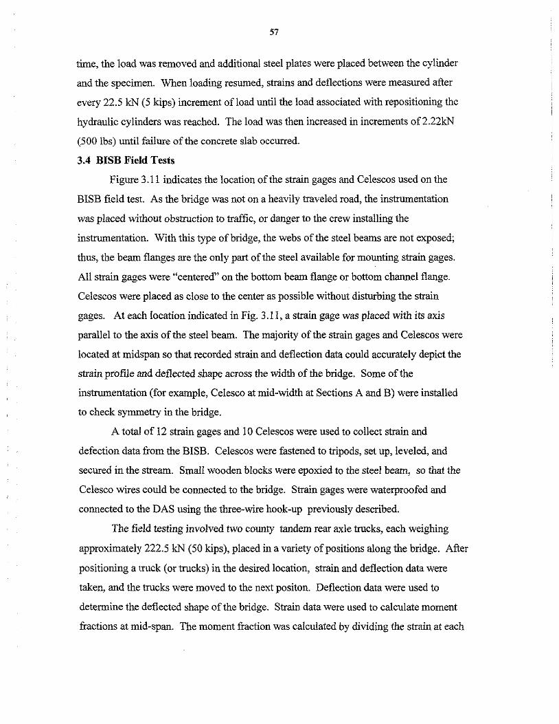
57
time, the load was removed and additional steel plates were placed between the cylinder
and the specimen. When loading resumed, strains and deflections were measured after
every 22.5 kN (5 kips) increment ofload until the load associated with repositioning the
hydraulic cylinders was reached. The load was then increased in increments of2.22kN
(500 lbs) until failure of the concrete slab occurred.
3.4 BISB Field Tests
Figure 3.11 indicates the location of the strain gages and Celescos used on the
BISB field test. As the bridge was not on a heavily traveled road, the instrumentation
was placed without obstruction to traffic, or danger to the crew installing the
instrumentation. With this type of bridge, the webs of the steel beams are not exposed;
thus, the beam flanges are the only part of the steel available for mounting strain gages.
All strain gages were "centered" on the bottom beam flange or bottom channel flange.
Celescos were placed as close to the center as possible without disturbing the strain
gages. At each location indicated in Fig. 3 .11, a strain gage was placed with its axis
parallel to the axis of the steel beam. The majority of the strain gages and Celescos were
located at midspan so that recorded strain and deflection data could accurately depict the
strain profile and deflected shape across the width of the bridge. Some of the
instrumentation (for example, Ce!esco at mid-width at Sections A and B) were installed
to check symmetry in the bridge.
A total of 12 strain gages and I 0 Celescos were used to collect strain and
defection data from the BISB. Celescos were fastened to tripods, set up, leveled, and
secured in the stream. Small wooden blocks were epoxied to the steel beam, so that the
Celesco wires could be connected to the bridge. Strain gages were waterproofed and
connected to the DAS using the three-wire hook-up previously described.
The field testing involved two county tandem rear axle trucks, each weighing
approximately 222.5 kN ( 50 kips), placed in a variety of positions along the bridge. After
positioning a truck (or trucks) in the desired location, strain and deflection data were
taken, and the trucks were moved to the next positon. Deflection data were used to
determine the deflected shape of the bridge. Strain data were used to calculate moment
fractions at mid-span. The moment fraction was calculated by dividing the strain at each
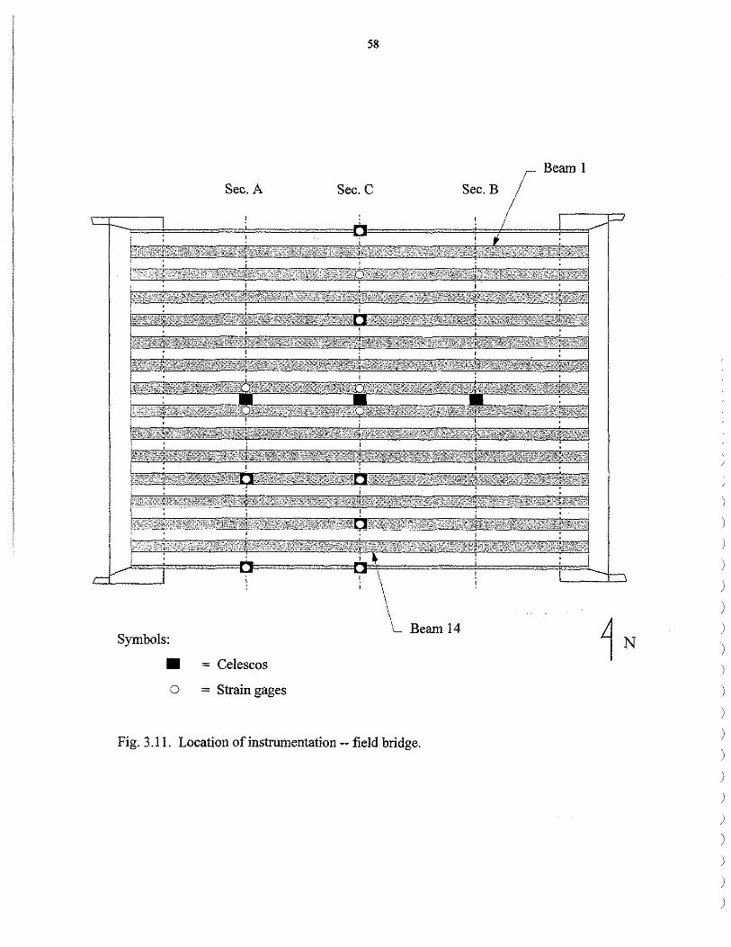
58
Sec.A Sec. C
Symbols: Beam 14
• = Celescos
o = Strain gages
Fig. 3 .11. Location of instrumentation -- field bridge.
Beam 1
Sec.B
)
)
)
)
)
)
)
)
)
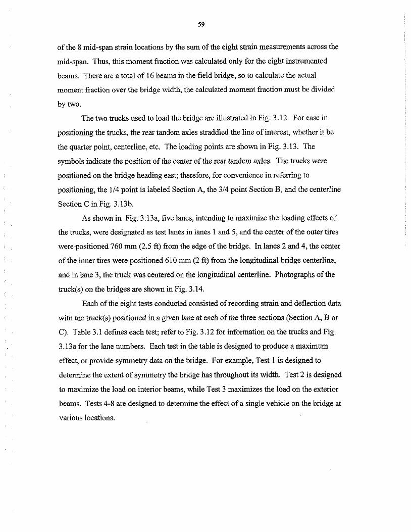
59
of the 8 mid-span strain locations by the sum of the eight strain measurements across the
mid-span. Thus, this moment fraction was calculated only for the eight instrumented
beams. There are a total of 16 beams in the field bridge, so to calculate the actual
moment fraction over the bridge width, the calculated moment fraction must be divided
by two.
The two trucks used to load the bridge are illustrated in Fig. 3.12. For ease in
positioning the trucks, the rear tandem axles straddled the line of interest, whether it be
the quarter point, centerline, etc. The loading points are shown in Fig. 3 .13. The
symbols indicate the position of the center of the rear tandem axles. The trucks were
positioned on the bridge heading east; therefore, for convenience in referring to
positioning, the 1/4 point is labeled Section A, the 3/4 point Section B, and the centerline
Section C in Fig. 3.13b.
As shown in Fig. 3 .l 3a, five lanes, intending to maximize the loading effects of
the trucks, were designated as test lanes in lanes 1 and 5, and the center of the outer tires
were positioned 760 mm (2.5 ft) from the edge of the bridge. In lanes 2 and 4, the center
of the inner tires were positioned 610 mm (2 ft) from the longitudinal bridge centerline,
and in lane 3, the truck was centered on the longitudinal centerline. Photographs of the
truck(s) on the bridges are shown in Fig. 3.14.
Each of the eight tests conducted consisted of recording strain and deflection data
with the truck(s) positioned in a given lane at each of the three sections (Section A, B or
C). Table 3 .1 defines each test; refer to Fig. 3 .12 for information on the trucks and Fig.
3. l 3a for the lane numbers. Each test in the table is designed to produce a maximum
effect, or provide symmetry data on the bridge. For example, Test 1 is designed to
determine the extent of symmetry the bridge has throughout its width. Test 2 is designed
to maximize the load on interior beams, while Test 3 maximizes the load on the exterior
beams. Tests 4-8 are designed to determine the effect of a single vehicle on the bridge at
various locations.
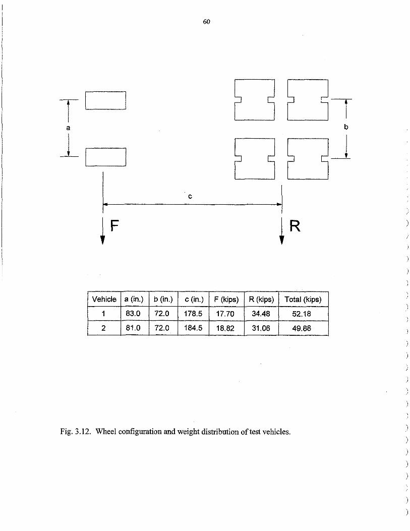
60
T .__I __J
a
_l
c
iF iR
Vehicle a (in.) b (in.) c (in.) F (kips) R (kips) Total (kips)
1 83.0 72.0 178.5 17.70 34.48 52.18
2 81.0 72.0 184.5 18.82 31.06 49.88
Fig. 3.12. Wheel configuration and weight distribution oftest vehicles.
b
_l
)
)
)
)
)
)
)
)
)
)
)
)
)

61
LANE3
[[}=={]]
I
! 30' Nominal
Bridge Centerline
a. Cross-section
50' - 2" r~~~~~~~~~~~~~~-i
'
I
I - - • - -I
I
- - ' - -
I
I - - • - -
I
I - - • - -
I
I
- - + - -I : I
' Sec A SecC SecB
b. Plan view
Fig. 3 .13. Location of test vehicles.
~I
Cent erline Lane I
Cent erline Lane 2
Cent erline Lane 3
Cent erline Lane 4
Cent erline Lane 5

62
a. Test vehicle in lane 3
b. Test vehicles in lanes 2 and 4
Fig. 3.14. Photographs oftest vehicles on bridge.
)
)
)
)
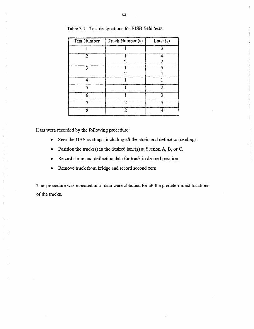
63
Table 3.1. Test designations for BISB field tests.
Test Number Truck Number (s) Lane (s)
1 1 3
2 1 4 2 2
3 1 5 2 1
4 1 1
5 1 2
6 1 3
7 2 5
8 2 4
Data were recorded by the following procedure:
• Zero the DAS readings, including all the strain and deflection readings.
• Position the truck(s) in the desired lane(s) at Section A, B, or C.
• Record strain and deflection data for truck in desired position.
• Remove truck from bridge and record second zero
This procedure was repeated until data were obtained for all the predetermined locations
of the trucks.
65
4. BEAM-IN-SLAB BRIDGE GRILLAGE ANALYSIS
The grillage method of analysis was selected for modeling the BISB system. The
tenn "grillage analogy" is used to describe an assembly of one-dimensional beams which
are subjected to load acting perpendicular to the plane of the assembly (16). Grillage
analysis differs from plane frame analysis in that the torsional rigidities are incorporated
into the analysis. To perfonn the analysis, a finite element program was used; ANSYS
5.3 (17) was chosen because it has a large number of different types of elements
available.
4.1 Element Types
The FEM of the BISB used two different types of elements for the components in
the bridge system. The element types are described in the ANSYS 5.3 Users Manual (17).
4.1.1 BEAM4 Element
From the ANSYS 5.3 Users Manual:
"BEAM4 is a uniaxial element with tension, compression, torsion, and bending capabilities. The element has six degrees of freedom at each node; translation in the nodal x, y, and z directions and rotations about the nodal x, y, and z axes."
"The geometry, node locations, and coordinate system are shown (see Fig 4.1). Th,,,. ""l"'""'""'ttt ;c.> A,,.f1n,,::.rl lnr hxrn n1' fh.,.ai.:i. nnrlaC' th,::. ,...,.ru:•c.<-o.:i.r-t1nn".ll1 "=11'P.<;lo +n.1n !:11'P~ .1.J.J. ..... lv,l...,,l.l.lVJ..U.- ,1.o.J ..,....,,,1..J.J.J.._,U. VJ .. YYV V.1. UMVV .U.V' ..... VU' W.J.V ..., ... .._,..,'-" .;>...,V .. J.V.O.J.U.J. ........ '-' .... , .. YYV w..L"" ....
moments of inertia (IZZ and IYY), two thicknesses (TKY and TKZ), an angle of rotation about the element x-axis, the torsional moment of inertia, and the material properties."
"The beam must not have zero length or area. The moments of inertia, however, may be zero if large deflections are not used. The beam can have any crosssectional shape for which the moments of inertia can be computed. The stresses, however, will be detennined as if the distance between the neutral axis and the extreme fiber is one-half of the corresponding thickness."
4.1.2 BEAM44 3-D Tapered Unsymmetric Beam Element
From the ANSYS 5.3 Users manual:
"BEAM44 is a uni-axial element with tension, compression, torsion, and bending capabilities. The element has six degrees of freedom at each node: translations in the nodal x, y, and z directions and rotations about the nodal x, y, and z axes (see Fig. 4.2). The element allows different unsymmetrical geometry at each end and pennits the end nodes to be offset from the centroidal axis of the beam."
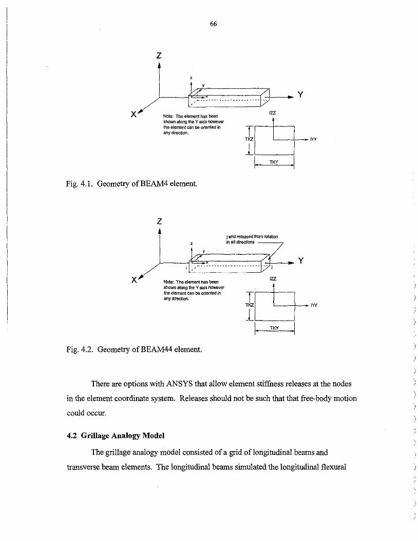
z
x
66
Note: The element has been shown along the Y axis however the element can be oriented in any direction.
Fig. 4.1. Geometry of BEAM4 element.
z
x No\e: The element has been ShOINl'l along the Y aX!s however the element can be oriented in any direction.
Fig. 4.2. Geometry ofBEAM44 element.
IZZ
'----+---IYY I 1'------'
1. TKY
j end released from rotation in all directions -----,
I 1
IZZ
'----+-- IYY
._I __ r_KY _ ___,
There are options with ANSYS that allow element stiffness releases at the nodes
in the element coordinate system. Releases should not be such that that free-body motion
could occur.
4.2 Grillage Analogy Model
The grillage analogy model consisted of a grid of longitudinal beams and
transverse beam elements. The longitudinal beams simulated the longitudinal flexural
)
)
)

67
stiffness and torsional stiffness of the steel beam and concrete deck, which is assumed to
have participated in the longitudinal load resistance. The ANSYS BEAM4 element was
used to characterize the longitudinal member. The transverse beams in the grillage
simulated the transverse stiffness and torsional stiffness of the concrete deck. The
ANSYS BEAM44 element was used to characterize the transverse member. A typical
grillage for the BISB system is shown in Fig. 4.3.
The response of the grillage model is affected by some basic parameters, such as
the spacing of the transverse beams, the end restraint of both the longitudinal and
transverse beams, and the section properties (flexural and torsional) of both the
longitudinal and transverse beams. To determine the appropriate choices for these
parameters, sensitivity studies were performed. Following are the parametric values used
in the study:
• Spacing of transverse beams at 5 mm, 8 mm, 15 mm, 30 mm, and 91 mm (2
in., 3 in., 6 in., 12 in., and 36 in.)
• Transverse beam end conditions (fixed and pinned).
• Transverse beam flexural stiffness (as a percentage of the contributory concrete
area).
• Longitudinal beam end condition (fixed and pinned).
• Longitudinal beam flexural stiffness.
• Longitudinal beam torsional stiffness.
Regarding the appropriate longitudinal flexural stiffness, three different values
were investigated. The modulus of elasticity of steel, E = 200 GPa (29 ,000 ksi), was used
and the moment of inertia was varied. The first value of the moment of inertia used was
that of the steel beam alone, without regard to any contribution from the concrete. The
second moment of inertia was based upon the calculated flexural stiffness of the two
beam BISB specimen, which is presented in the next chapter. The third value was based
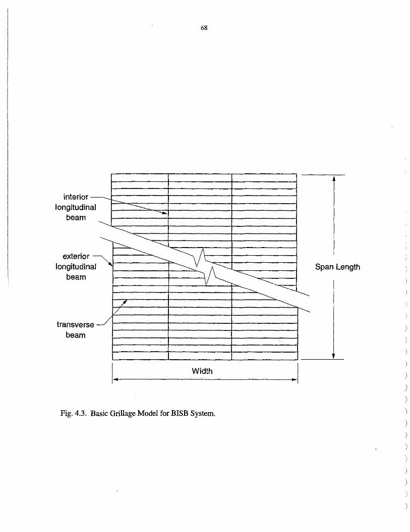
interior longitudin
beam
"--
exterior longitudin
beam
al
~ al ~
transverse beam
-----,....___
68
--- ~
------------
------
~;::::_------
Width
Fig. 4.3. Basic Grillage Model for BISB System.
Span Length
)
)

69
upon recommendations by Jaeger and Bakht for slab and girder bridges (16). Their value
assumes complete composite action between the concrete (based on contributory area)
and the steel, and uses a transformed value for the entire concrete section. The modulus
of elasticity of the concrete used for this and all subsequent transformations was E = 29
GPa ( 4,200 ksi). Note that different values were calculated for the exterior and interior
longitudinal beams because of the different amounts of contributing concrete. For the
exterior beams, the moments of inertia for the three cases were 1.76 x 108 mm4
(662 in\
3.08 x 108 mm4 (740 in\ and 3.50 x 108 mm4 (840 in\ For the interior beams, the
moments of inertia were 1.76 x 108 mm4 (662 in\ 3.41x108 mm4 (820 in\ and 4.25 x
108 mm4 (1020 in\
The torsional stiffness of the longitudinal beams was also studied by using the
modulus of elasticity of steel and by varying the torsional moment of inertia. The first
value assumed that the steel beam had a value of 1.60 x 106 mm4 (3.84 in\ A second
value based on recommendations by Jaeger and Bakht assumed that all of the concrete
contributed to the torsional stiffness of the specimen, and a transformed section was used
to calculate the torsional moment of inertia. The value of the torsional moment of inertia
for the entire section was 6.24 x 10⁷ rnm4 (150 in\ A third value midway between these
two was also selected, resulting in a torsional stiffness of3.12 x 107 mm4 (75 in\
The transverse beam properties were investigated assuming that only the
contributory region concrete contributed strength. The study considered varying
percentages (10 %, 25%, 50%, 75%, 90%, and 100%) of the transverse beam width
(which varied depending on the assigned spacing of the transverse beams) as contributing
to the transverse beam stiffuess.
The sensitivity of the analytical response of a BISB system based on the four
beam BISB specimen described in Chp 2 of this report was also studied. In each of these
analyses, an 89 kN (20 kips) load was applied at midspan of an exterior beam. The
deflection data shown refer to the midspan deflections of each of the four beams. Figure
4.4a shows the effect of the transverse beams spacing. Large spacing increases the
transverse stiffuess. In Fig. 4.4b., the effect of the connection between the transverse and
longitudinal beams is illustrated. As shown, the fixed connection has a greater transverse

70
--0.12,-----------;::======:::;-----------:::::i
1
2" ~ 6" 12" 3~"1 . -e- =- v -11(- -,- . --0.14
.Ql6
--0.26'-'-----------2;,---------~3----------+'4
Beam Number a. Transverse beam spacing
--0.05,------------~==:::;--------------i Pinned F'JXed
-0.] - -e-B
.E .o.1s r- :i-------~/7.f'.l:::=;:::::::::::::::::::::::=---f3---------1 1--02~
--0.3
-0.35 c;-.---------2;,-----------±-3---------"'"4 Beam Number
b. Transverse beam end conditions
0.1-----------------------------~
0.05
.5 oc==~====s==-====1 i:::::"' -Cl.OS 0 ,_
·g -OJ w 1i
Cl --0.ISr >-----------<~;i----------e-----------0.2~ ~
--0.25 c+-----------c;,----------*"' ·------------';' 2 3 4 Beam Number
c. Longitudinal beam end conditions
Fig. 4.4. Sensitivity study results for basic parameters.
)
)
)
)
)
)
)
)
)
)
)
)
)

71
stiffness than the pin connection. The effect of the longitudinal beam support conditions
is shown in Fig. 4.4c and, as expected, the deflections are significantly smaller when
fixed end conditions are used.
The results of the study on the section properties for the transverse and
longitudinal beams are shown in Fig. 4.5. As can be seen in Fig. 4.5a, the change in
properties for the transverse members (defined as a percentage of the contributory
concrete area) has a significant effect on the load distribution characteristics of the model.
As expected, the larger the percentage of section used to determine the transverse beam
properties, the greater the transverse load distribution. Figure 4.5b shows the variation
among the three values for the flexural stiffness of the longitudinal beams. Figure 4.5c
illustrates the effect of the different values of torsional moment of inertia upon the model.

72
(0.1),----------;::========;----------, (0.12)
(0,14)
.s (0.16)
·~ (O.!S)
i:l ~ (02) 0
(0.22) !~-"""""~~~~~ (0,24)
10% 25% SO"h 75% 90"/o 100% *-8- -El -0--+-*
(0,26) =------------'-------------'-----------LJ 2 3 4
Beam Number a. Transverse beam properties
(O.l)
l 66~~ 8 "4 102~"4 I /
-(0.!5) A
v ,... A . v w -v
L'.T --(0.3) ~
' 2 3 4
(0.35)
Beam Number b. Longitudinal beam flexural stiffi:tess
(O.OS)r------------;::=====:::;------------, 4 in."4 75in."4 ISO in."4
(O.I) -e-- -8- ~
.5
i:f (0.!5) l.-------=::::::~~~;;?"""'_.-,a=::::;'::~~=====------~1 j (0.2)
Cl
(0.3) "-----------'-----------~---------....W 2 3 4
Beam Number c. Longitudinal beam torsional stiffi:tess
Fig. 4.5. Sensitivity studies for beam properties. )
)
)
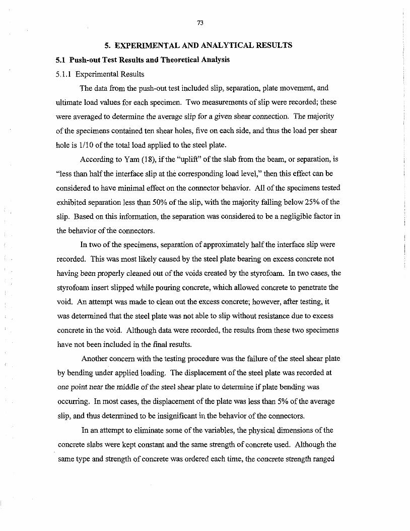
73
5. EXPERIMENT AL AND ANALYTICAL RESULTS
5.1 Push-out Test Results and Theoretical Analysis
5 .1.1 Experimental Results
The data from the push-out test included slip, separation, plate movement, and
ultimate load values for each specimen. Two measurements of slip were recorded; these
were averaged to determine the average slip for a given shear connection. The majority
of the specimens contained ten shear holes, five on each side, and thus the load per shear
hole is 1/10 of the total load applied to the steel plate.
According to Yam (18), if the "uplift" of the slab from the beam, or separation, is
"less than half the interface slip at the corresponding load level," then this effect can be
considered to have minimal effect on the connector behavior. All of the specimens tested
exhibited separation less than 50% of the slip, with the majority falling below 25% of the
slip. Based on this information, the separation was considered to be a negligible factor in
the behavior of the connectors.
In two of the specimens, separation of approximately half the interface slip were
recorded. This was most likely caused by the steel plate bearing on excess concrete not
having been properly cleaned out of the voids created by the styrofoam. In two cases, the
styrofoam insert slipped while pouring concrete, which allowed concrete to penetrate the
void. An attempt was made to clean out the excess concrete; however, after testing, it
was determined that the steel plate was not able to slip without resistance due to excess
concrete in the void. Although data were recorded, the results from these two specimens
have not been included in the final results.
Another concern with the testing procedure was the failure of the steel shear plate
by bending under applied loading. The displacement of the steel plate was recorded at
one point near the middle of the steel shear plate to determine if plate bending was
occurring. In most cases, the displacement of the plate was less than 5% of the average
slip, and thus determined to be insignificant in the behavior of the connectors.
In an attempt to eliminate some of the variables, the physical dimensions of the
concrete slabs were kept constant and the same strength of concrete used. Although the
same type and strength of concrete was ordered each time, the concrete strength ranged
74
from 34.70 MPa (5,040 psi) to 56.85 MPa (8,250 psi). Therefore, the experimental
results are presented, along with results normalized for a concrete strength of 41.35 MPa
(6,000 psi). Since shear is the main mechanism of failure, the f is used to convert
the measured data to normalized data. This is done by using the following expression:
Normalized value= Measured value x [6,000 psi/(fc,)J112 (5.1)
where ( is the actual concrete compressive strength, and 6,000 psi is the desired concrete
compressive strength. Normalizing the concrete strengths allowed for a direct
comparison of the variables in the various series. Complete results are shownin Table
5 .1. Results from Series 6 have been neglected due to inconsistent fabrication of the
specimens. The reinforcing bar placed in the middle shear hole was welded instead of
simply placed in the hole, thus preventing movement of the reinforcing bar. The average
for the normalized maximum load for Series 6 was 465.5 kN (104.6 kips), a value that is
too large based on the maximum loads of Series 4, 8, 9, and 10.
Results in Table 5.1 indicate that Series 4, 8, 9, and 10 far exceeded the load
carrying capacity of the other series. All ofthe specimens in Series 4, 8, 9, and 10 were
at or near 445 kN (100 kips) for the normalized maximum load. Initial slip data,
however, showed that the connections without reinforcement through the shear holes
provided a stiffer connection. Series 1, without reinforcement through the shear holes,
had an initial slip of 1,275 kN/mm (7,290 kip/in.), whereas values for Series 4, 8, 9, and
10, with reinforcement through the shear holes, varied from 795 kN/mm (4,550 kip/in.) to
990 kN/mm (5,650 kip/in.). Therefore, although the reinforcing bar added strength to the
shear connection, the reduction in shear hole area by inserting the reinforcement in the
hole reduced the stiffuess of the shear connection.
)
)
)
)
)
)
)
)

Table 5.1. Push-out test results.
Series ( (psi)
1 6790
2 8250
3 8250
4 6480
5 6480
7 5380
8 5040
9 5040
10 5500
11 5500
Note: 1 psi= 6.89 kPa l kip= 4.45 k.N
Maximum Load
(kips)
77.8
91.0
60.2
98.8
84.2
7.7
86.5
92.l
89.7
40.0
75
Initial Slip Maintenance at
(kip/in. x 0.3 in. Slip 103
) Percent of Maximum Load
7.29 90.l
8.75 81.9
4.40 79.2
5.43 89.4
5.68 85.9
-- 73.3
5.10 75.4
5.65 81.7
4.55 91.5
-- 88.3
l kip/in. = 0.175 kN/mm l in.= 25.4 rnm
Normalized
Maximum Load
(kips)
73.l
77.6
51.3
95.l
81.0
8.1
94.4
100.5
93.7
41.8
It can also be seen in Table 5.1 that all of the specimens maintained a large
percentage of the maximum load up to an average slip of7.6 mm (0.3 in.). It was at this
point in the tests that the load carrying capacity of the shear connection began to decrease
rapidly in the weaker connections, and thus an average slip of7.6 mm (0.3 in.)was
selected as the magnitude of slip for load maintenance after failure of the shear
connection.
Figure 5.1 presents a comparison of the variables investigated as follows: size of
holes, spacing of holes, alignment of holes, inclusion of reinforcing steel in holes, and
effects of "sloppy" craftsmanship. These graphs are based on a normalized concrete
strength of 41.35 MPa (6,000 psi). Three items of interest may be observed in these
graphs. First, all of the specimens with shear holes demonstrated a nearly linear phase up
to the point of maximum load. This linear phase is noted as the initial slip in Table 5 .1,
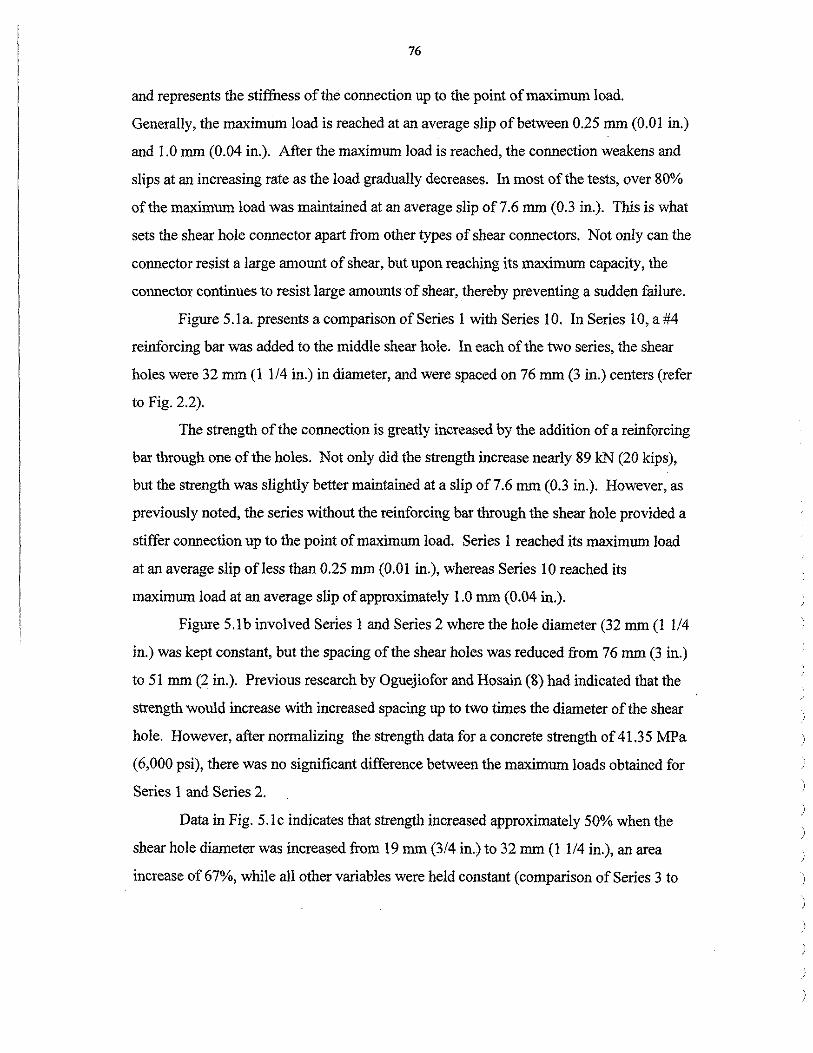
76
and represents the stiffness of the connection up to the point of maximum load.
Generally, the maximum load is reached at an average slip of between 0.25 mm (0.01 in.)
and 1.0 mm (0.04 in.). After the maximum load is reached, the connection weakens and
slips at an increasing rate as the load gradually decreases. In most of the tests, over 80%
of the maximum load was maintained at an average slip of7.6 mm (0.3 in.). This is what
sets the shear hole connector apart from other types of shear connectors. Not only can the
connector resist a large amount of shear, but upon reaching its maximum capacity, the
connector continues to resist large amounts of shear, thereby preventing a sudden failure.
Figure 5.la. presents a comparison of Series 1 with Series 10. In Series 10, a #4
reinforcing bar was added to the middle shear hole. In each of the two series, the shear
holes were 32 mm (1 1/4 in.) in diameter, and were spaced on 76 mm (3 in.) centers (refer
to Fig. 2.2).
The strength of the connection is greatly increased by the addition of a reinforcing
bar through one of the holes. Not only did the strength increase nearly 89 kN (20 kips),
but the strength was slightly better maintained at a slip of7.6 mm (0.3 in.). However, as
previously noted, the series without the reinforcing bar through the shear hole provided a
stiffer connection up to the point of maximum load. Series 1 reached its maximum load
at an average slip ofless than 0.25 mm (0.01 in.), whereas Series 10 reached its
maximum load at an average slip of approximately 1.0 mm (0.04 in.).
Figure 5.1 b involved Series 1 and Series 2 where the hole diameter (32 mm (1 1/4
in.) was kept constant, but the spacing of the shear holes was reduced from 76 mm (3 in.)
to 51 mm (2 in.). Previous research by Oguejiofor and Hosain (8) had indicated that the
strength would increase with increased spacing up to two times the diameter of the shear
hole. However, after normalizing the strength data for a concrete strength of 41.35 MPa
(6,000 psi), there was no significant difference between the maximum loads obtained for
Series 1 and Series 2.
Data in Fig. 5. lc indicates that strength increased approximately 50% when the
shear hole diameter was increased from 19 mm (3/4 in.) to 32 mm (11/4 in.), an area
increase of 67%, while all other variables were held constant (comparison of Series 3 to
' )

.. Q. :ii ..; "' 0 ..J
.. a. :ii ..; "' 0 ..J
77
100 ·.
90
~r 80
70
Series IO
1~
60 Series 1
50 .
40
30
20
10
0 0 0.05 0.1 0.15 0.2
Slip, in.
a. Load slip curves for Series 1 and 10
100
90 ~
80 .~ f\. ...-... / Series 2
70
60 .
50 .
40 .
30
20.
10 .
0
~Series I
0.05 0.1 0.15
Slip, in.
0.2
b. Load slip curves for Series 1 and 2
Fig. 5 .1. Load slip curves for various test sequences.
0.25 0.3
0.25 0.3
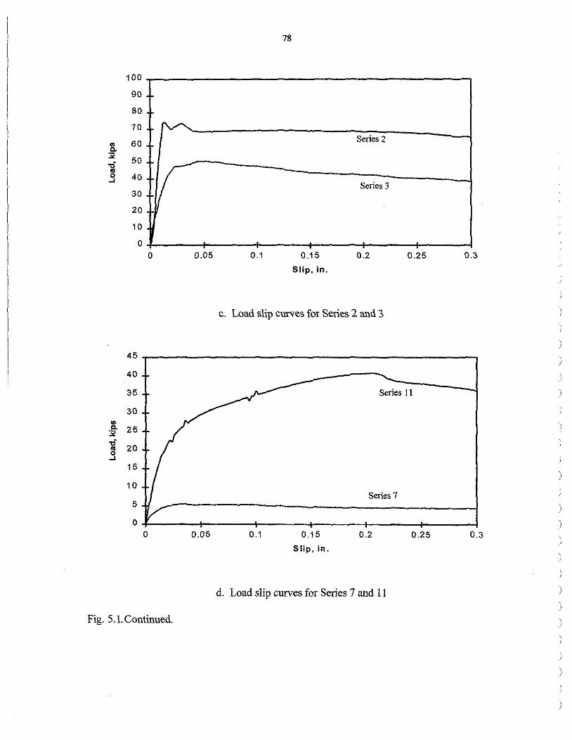
100
90 . -
80 --
70 . - l'\r"'...
~ 60 :.;;:
50 . -0
:1r .. 0 40 . ..J
30.
20.
10
0 0
45
40
35
30
"' c. 25 :.;;: -0
20 "' 0 ..J
15
10
5
0 0
Fig. 5.1. Continued.
0.05
0.05
78
0.1 0.15
Slip, in.
Series 2
Series 3
0.2
c. Load slip curves fo; Series 2 and 3
0.25
Series 11
0.1 0.15
Slip, in.
Series 7
0.2
d. Load slip curves for Series 7 and 11
0.25
0.3
0.3
)
)
)
)
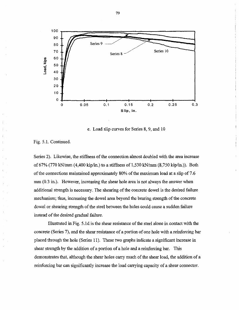
79
100
90 ••
1/ 80 • - Series 9
70 • -Series 8
Series 10
I/) 60 • -0. :;:
50 • -c ., 0 40 • .J
30 •
20 •
10 •
0 0 0.05 0 .1 0.15 0.2 0.25 0.3
Slip, in.
e. Load slip curves for Series 8, 9, and 10
Fig. 5.1. Continued.
Series 2). Likewise, the stiffness of the connection almost doubled with the area increase
of 67% (770 kN/mm (4,400 kip/in.) to a stiffuess of 1,530 kN/mm (8,750 kip/in.)). Both
of the connections maintained approximately 80% of the maximum load at a slip of 7 .6
mm (0.3 in.). However, increasing the shear hole area is not always the answer when
additional strength is necessary. The shearing of the concrete dowel is the desired failure
mechanism; thus, increasing the dowel area beyond the bearing strength of the concrete
dowel or shearing strength of the steel between the holes could cause a sudden failure
instead of the desired gradual failure.
Illustrated in Fig. 5 .1 d is the shear resistance of the steel alone in contact with the
concrete (Series 7), and the shear resistance of a portion of one hole with a reinforcing bar
placed through the hole (Series 11 ). These two graphs indicate a significant increase in
shear strength by the addition of a portion of a hole and a reinforcing bar. This
demonstrates that, although the shear holes carry much of the shear load, the addition of a
reinforcing bar can significantly increase the load carrying capacity of a shear connector.
80
Neither of these two graphs demonstrate the linear relationship between load and slip up
to maximum load, and therefore the stiffness of the corresponding series cannot be
compared.
Lastly, a series oftests were completed, varying only the manner in which the
holes were manufactured. Data from specimens with drilled holes (Series l 0), torched
holes (Series 8), and poorly torched holes (Series 9) are compared in Fig. 5 .le. After
adjusting the results for a concrete strength of 41.35 Mpa (6,000 psi), the maximum loads
for all the specimens in this sequence were within 8% of each other. The slightly higher
strength associated with the torched holes could be due to a small increase in the hole
area caused by the inaccuracies associated with torching rather than drilling. In addition,
the stiffness of all three series were within 20% of each other. The lower values
associated with maintenance of the maximum load for Series 8 and 9 (75.4% and 81.7%,
respectively) in comparison with Series 10 (91.5%) could be explained by the lower
concrete strength in Series 8 and 9 (34.7 Mpa (5,040 psi) compared to 37.9 Mpa (5,500
psi)) for Series 10.
5.1.2 Analysis of Experimental Results and Development of Strength Equation
From the results of the tests, it was determined that the strength of the ASC was
influenced by five items: concrete compressive strength, the friction between the steel
plate and the concrete, the concrete dowel formed by concrete, the reinforcing bar placed
through the shear hole, and the transverse slab reinforcing. From the results of the
pushout tests, it was determined that hole spacing was not an important influence on the
strength of the connection if the spacing was at least 1.6 times the hole diameter.
Therefore, spacing of the shear holes was not included in the design equation; the design
equation is only valid for hole spacings greater than 1.6 times the shear hole diameter.
Using data from the push-out tests, an equation was developed that can predict the shear
strength of the ASC.
To determine the shear capacity of a stud connector based on the resistance of the
concrete slab to longitudinal splitting, Davies (10) developed the following equation:
)
)
)
)
)
)
)
)
)
)
)

81
where:
q = shear capacity per perfobond rib connector, lbf.
A,,= shear area of concrete per connector, in2.
u,. = concrete cube strength, psi.
Art= area of transverse reinforcement, in2•
fyr = yield strength of reinforcement, psi.
(5.2)
The longitudinal splitting of the specimens in tests performed by Davies is similar
to that observed in the push-out tests in this investigation. Therefore, his equation was
used as a basis for deriving a similar equation for the ASC.
The two terms of Davies' equation account for the contribution of the concrete
slab and the transverse reinforcement, respectively. Since the push-out specimen are
subjected only to direct stress, the potential of the slab to resist longitudinal splitting
would be dependent on the concrete strength, and the amount and strength of transverse
reinforcement. In addition, this investigation plus those of other researchers have shown
t.liat t.lie concrete do,x1el formed through the shear hole, as \Vel! as a reir1forcing bar placed
through the hole, will contribute to the capacity of the shear connection. Therefore, a
modification of the equation developed by Davies to incorporate these additional strength
parameters was developed. This modified equation follows:
where:
A,= Total area of steel in contact with the concrete, in2.
f 'c = Concrete compressive cylinder strength, psi.
A, = Area of reinforcing bar through shear holes, in2 per five holes.
fyr =Yield strength of reinforcing bar, psi.
Atr =Area of transverse reinforcement per hole divided by two, in2•
(5.3)

82
fy1r= Yield strength of the transverse reinforcement, psi.
Acd= Shear area of each concrete dowel, in2.
n = Number of concrete dowels.
q =strength of ASC, lbs.
p1, p2, p3, p4 =constants.
The equation has been modified to include the more traditional concrete compressive
strength, ( , instead of the cube strength, llw· The term Atr has been divided by two
because two layers of transverse reinforcement were used in the design of the push-out
specimens. A diagram illustrating the variables A,, A" and Acd is shown in Fig. 5.2.
1
Fig. 5.2. Illustration of equation variables.
The equations for As,, and Acd are as follows:
A, = 2(bl - 4A1 - A2)
Acd = 2(nd2/4)
T b
1
(5.4)
(5.5)
By reviewing beam sizes that might be used for bridge stringers, it was
determined that the smallest web thickness that might be encountered in the field would
be approximately 9.5 mm (3/8 in.). Therefore, steel plate thickness was not included as a
variable; the expression developed will thus result in conservative strength values for web
)
)
)
)
)

83
variable; the expression developed will thus result in conservative strength values for web
thicknesses greater than 9.5 mm (3/8 in.). Additionally, as previously noted, the holes
must be spaced at least 1.6 times the diameter of the shear hole so that the stress fields do
not overlap, causing a decrease in strength.
The p1, P2, P3, and P4 in Eqn. 5.3 are constants that were determined statistically
from the experimental results. The personal computer version ofMathcad was used to
solve for the most fitting equation from the experimental data. For each series, the
experimental strength was used as strength q in Eqn. 5.3, and the constants, p1, P2, P3, and
P4, were determined for the geometry of each shear hole connection. The values of these
constants were determined as follows: P1 = 0.618, P2 = 0.354, P3 = 0.353, 134 = 19.050
to three decimal places. Practical values of these constants which lower the theoretical
strength, q, by approximately 0.5% are used in Eqn. 5.6, which may be used to predict the
shear strength of this type of connector.
(5.6)
Since the concrete dowels are subjected to double shear, the term Acd , the total
shear area, would be calculated as 2(7t d2/4) where dis the diameter of the shear hole in
inches. Likewise, the steel is in contact with the concrete on both sides; thus, A, is two
times the cross-sectional area of the steel in contact with the concrete. If different areas
are used in the same shear connector, Eqn. 5.6 can be modified using n1 (number of holes
of area 1 ), n2 (number of holes of area 2), etc., so that only the portion of Eqn. 5.6 in
parentheses needs to be modified.
Comparisons of the results obtained from the preceding analysis to actual strength
data are presented in Table 5.2. Series 6 is excluded from the table for previously stated
reasons. Series 7 and 11 are also excluded from the table, as these two series were only
performed to obtain information on the steel-concrete friction (Series 7) and to determine
the effect of passing the reinforcement through the shear holes (Series 11 ).
As can be seen, Eqn. 5.6 accurately predicts the strength of the ASC to within
l 0% of the measured strength in most cases. Note that Eqn. 5 .6 provides failure

84
strengths. Thus, an appropriate factor of safety will be needed before the equation values
can be used in design.
Table 5.2. Theoretical Strengths vs. Experimental Strengths.
Series Experimental Theoretical Percent Difference
Number Strength Strength
(kips) (kips)
1 77.8 88.3 -13.60
2 . 91.0 93.0 -2.28
3 60.2 66.7 -10.66
4 98.8 87.1 11.80
5 84.2 87.l -3.33
8 86.5 84.0 3.00
9 92.l 84.0 9.50
10 89.7 85.6 4.67
5 .1.3 Sensitivity Study of Theoretical Strength Equation
An analysis was conducted to determine the contribution of each of the four terms
in Eqn. 5.6. The results of this part of the sensitivity study are presented in Table 5.3.
Overall, Terms 1-4 contribute an average of 8.9%, 2.6%, 50.8%, and 38.2%,
respectively, to the theoretical strength of the ASC. As can be seen, Term 2 could
conservatively be eliminated from Eqn. 5.6 without significantly reducing the theoretical
strength.
Equation 5 .6 involves five variables, which influence the shear strength of the
ASC: hole size, amount of reinforcing steel through the shear holes, amount of transverse
slab reinforcement, concrete strength, and number of shear holes. To determine the
influence of these variables, several sensitivity analyses were completed and presented in
Figs. 5.3-5.6.
)
)
)
)
)
)

85
Table 5.3. Results of sensitivity investigation.
Series Tenn 1 Tenn2 Tenn3 Tenn4 Total Strength
Number (kips) (kips) (kips) (kips) (kips)
1 7.4 0 42.4 38.6 88.3
2 8.2 0 42.4 42.5 93.0
3 9.0 0 42.4 15.3 66.7
4 7.3 2.3 42.4 35.l 87.l
5 7.3 2.3 42.4 35.l 87.l
8 6.5 4.2 42.4 30.9 84.0
9 6.5 4.2 42.4 30.9 84.0
10 6.7 4.2 42.4 32.3 85.7
Note: Tenn I = 0.62 A, F Tenn 3 = 0.35 nAuf1r
Tenn 2 = 0.35 A,f, Tenn 4 = 19 nAcd F Figure 5 .3 shows the sensitivity of the shear strength to an increase in the shear
hole area. In this figure, the reinforcement included in the shear holes was constant at
130 mm2 (0.2 in2) (#4 reinforcing bar), and the area of transverse reinforcement (A,,) was
held constant at 130 mm2 (0.2 in2). A total often shear holes were included in the
analysis (simulating Series 10 push-out tests). Five different concrete compressive
strengths were examined to determine the effect of concrete strengths on the strength of
the ASC. As can be seen in Fig. 5.3, as the hole area increases, the shear strength also
increases in a nearly linear fashion. It also can be observed that the concrete strength has
a direct influence on the shear strength.
In Fig. 5.4, the hole area was kept constant at 3,690 mm2 (5.72 in2) per five holes
(Series 10), and the area of transverse reinforcement (A1r) was held constant at 130 mm2
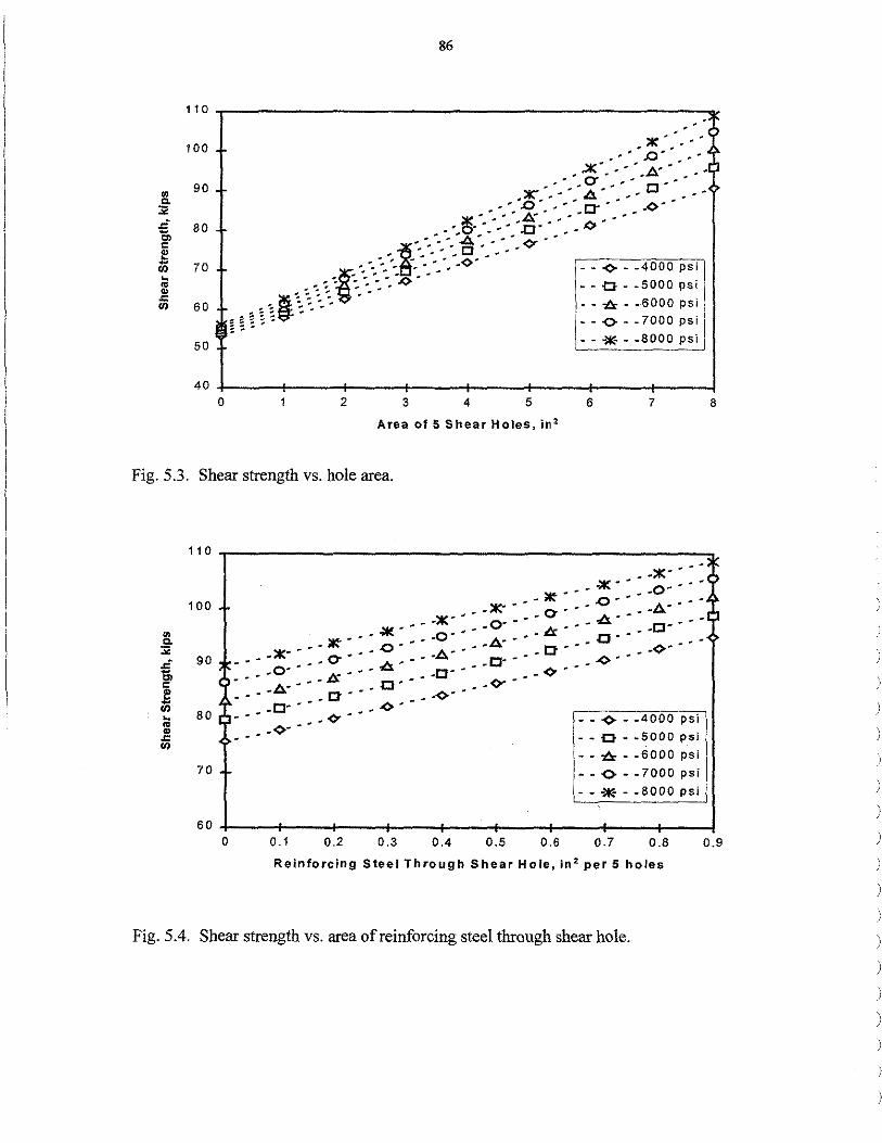
86
• • • c , :I: • • ••
100 ... • ..• : .0 •••..•• . x . . . .A: • • • ]
. 0- • . )K'·:.-·.o."'..CJ .. ••
• • 'J::> • ••• er . . .<>· 90 ...
• ~::-::-~:- .. _. ¢ ..•.
-tr:- · . .--:-8 ·:. ·:. <Y •••
70 L a". •:.:·.,5::-.-:.<>· • • -.-.--(>----_-4-0-00_p_s_i
-~ : • •• • ".<>·. - - o - -5000 psi
60 c • , ~f:\\\ ·- ·... , ---:ts: - -6000 psi
nn° - 1:·-<>--7000psii - - -:!!- - -8000 psi I 50 . ~ . '
80 -
0 2 3 4 5 6 7 8
Area of 5 Shear Holes, in 2
Fig. 5.3. Shear strength vs. hole area.
• -ll<- • - - , • .;:ic:·· ___ ,,
- - ~ . - - .o . . - .o· . - "• . · - .:t:·. _ - Ct - - - ,.. - - - -A- - ]
- • -lK o- · - · · """ c· · · • • .;:ic:· •• o···· .. . a o·· - _.,
100 .•
___ .;:i:- _ • .o-· .. -A .o··· .-<»"' so.c •• -·:t: .o· .. -·A .c--· _4··
:< _.o··· __ .-A .c--· _9-· ,.. _. •. Js. o--- .. <>-"
. - .A ct - - - ·<>" • .• c---- ¢•"" 80 ]---- •• ¢'···
-<>- -.~ ....
70 . ~
0 0.1 0.2 0.3 0.4 0.5 0.6
- - -<> - -4000 psi - - o - -5000 psi
. . -:ts: _ -6000 psi I I 0 -1··<>--70 Ops1 : . * .. sooo psi I
0.7 0.8 0.9
Reinforcing Steel Through Shear Hole, in 2 per 5 holes
Fig. 5 .4. Shear strength vs. area of reinforcing steel through shear hole.
)
)
)
)
)
)
)
)
)

87
(0.2 in2). As the amount of reinforcing steel in the shear hole increases, so does the shear
strength. However, the equation is not very sensitive to an increase in reinforcing steel in
the shear hole, as the strength only increases 8.9 kN (2 kips) for every additional 65 mm2
(0.1 in2) of reinforcing steel.
In Fig. 5.5, the hole area and the reinforcing steel through the shear hole were kept
constant at 3,690 mm2 (5.72 in2) and 130 mm2 (0.2 in\ respectively. The area of
transverse slab reinforcement was varied from no reinforcement to 645 mm2
(1.0 in2) of
reinforcing steel per shear hole. The graphs indicate that the shear strength of the
connection is significantly influenced by the amount of transverse slab reinforcing used.
Normally, however, this would not be a consideration, as the amount of transverse
reinforcing required would be determined using Eqn 1.4.
In Fig. 5.6, the reinforcing steel through the hole and the transverse reinforcing
steel were kept constant at 130 mm2 (0.2 in2) and 130 mm2 (0.2 in2
), respectively. The
number of shear holes was varied, assuming an area of795 mm2 (1.23 in2) per shear hole
(diameter of32 mm (1 114 in.)). The shear strength of the connection depends
significantly on the shear hole area, as can be seen by the increase in shear strength of
approximately 44.5 kN (10 kips) for every two additional shear holes.
Based on this sensitivity analysis, the shear hole area, the amount of transverse
reinforcement, the number of shear holes, and the concrete compressive strength are the
four primary factors that influence the shear strength of the ASC.
5.2 BISB Laboratory Test Results and Analysis
5.2.1 Two-Beam Specimen
The purpose of the BISB tests was to obtain strength and behavior data.
Deflection data as well as strain data collected during the testing of the specimen will be
presented and analyzed in this section. The loads presented in the following discussion
and graphs represent the load applied at each of the two loading points. The total load
applied to the structure is the sum of the two applied loads. The specimen supported a
load of approximately 445 kN (100 kips) applied to each loading point which was the
capacity of the loading frame. Non-linear strain behavior occurred at 267 kN (60 kips);
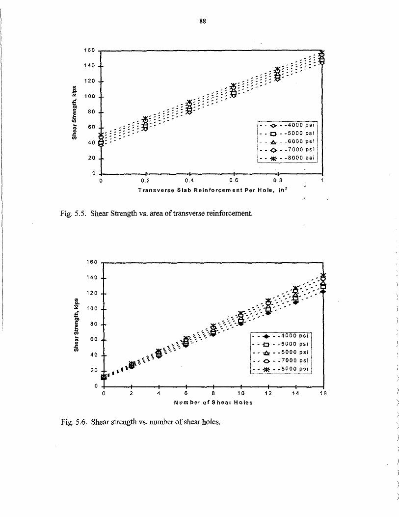
88
160
140
120
"' c. :;;: 100 .Ji -"' c 80 I!! -"' - 60 !,') .::
"' 40 - - -J::r - -6000 psi
- - O - -7000 psi 20 -. * --8000 psi
0 0 0.2 0 .4 0.6 0.8
Transverse Slab Reinforcement Per Hole, in 2
Fig. 5.5. Shear Strength vs. area of transverse reinforcement.
160
140
120
"' Q.
:;;: 100
i c 80 I!! (i) ~ 60 .. " .::
"' 40
20 I I
0 0
. . . ·. f:::::-::
. ·. ·-:~t::::::-: .... , . ·.o·-:·:·:
~:- '-\\~- .. ,i!S' ,._<._"·;·-~-:-:-. --+ - -4000 psi
• • ''fi'"· ._ • - - O - .5000 psi ~~\'::.'" • - .:e,, - -6000 psi
i~\· .. Mt,\<' --o--7000psi
1 I,.. . . * --8000 psi
2 4 6 8 10 12 14
Number of Shear Holes
Fig. 5 .6. Shear strength vs. number of shear holes.
16
)
)
)
)
)
)
' J
)
)

89
measurable end slip occurred at approximately 178 kN (40 kips). These loads are both
well above service loading conditions.
Experimental strains due to vertical loads are presented in Fig. S. 7. As previously
noted, strain gages were placed on the top and bottom flanges, as well as at the
approximate neutral axis of the composite section. In theory, the strain at the neutral axis
will be zero as long as the section remains composite. As the concrete in tension starts to
crack, the neutral axis will rise, which will be indicated by an increase in the strain at the
location of the composite neutral axis. As the concrete cracks, there will be a decrease in
composite action, rendering the concrete useless in terms of strength. This phenomenon
is indicated in the experimental results presented in Fig. 5.7.
The top and bottom beam flange strains in a non-composite structure should be of
approximately the same magnitude, but opposite sign, indicating the neutral axis is near
the center of the girder. By this logic, Fig. 5. 7 indicates that the specimen tested exhibits
the behavior of a non-composite beam. A closer inspection of the results is necessary,
however, as this behavior could be misleading. The concrete in the specimen tested filled
the void between the girders; thus, the neutral axis for the composite section was
approximately the same as the neutral axis of the non-composite section. Inspection of
the deflection data, presented later, will provide more information on composite action in
the tested specimen.
A "snapshot" of the strains across the depth of the cross section is shown in Fig.
5 .8 for both the quarter point and the centerline. The concrete did not visually show any
substantial cracking up to a load of 178 kN ( 40 kips) at each loading point; thus, the
strain at the composite neutral axis should be zero. Data in Fig. 5 .8 verify this. Likewise,
in the elastic range, the steel strain also increased in a linear fashion.
As previously mentioned, measurable end slip did not occur until the load reached
approximately 178 kN (40 kips) on each load point (see Fig. 5.9). This is apparently the
load at which the bond between the steel and concrete was broken. Note the rate at which
the concrete slipped once the steel-concrete bond was broken. This is a potential problem
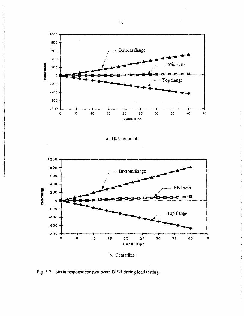
90
1000
800
600 L Bottomfl""" 400
.s Mid-web I! 200 -e ~
0
-200
-400
-600
-800 0 5 10 15 20 25 30 35 40
Load, kips
a. Quarter point
1000 l 800
600
400
" 1! 200 1i! 2 0 "
L., Mid-web
:ii -200
-400 ~ Top flange
-600
-800 0 5 10 15 20 25 30 35 40
Load, kips
b. Centerline
Fig. 5. 7. Strain response for two-beam BISB during load testing.
45
45
)
) \ )
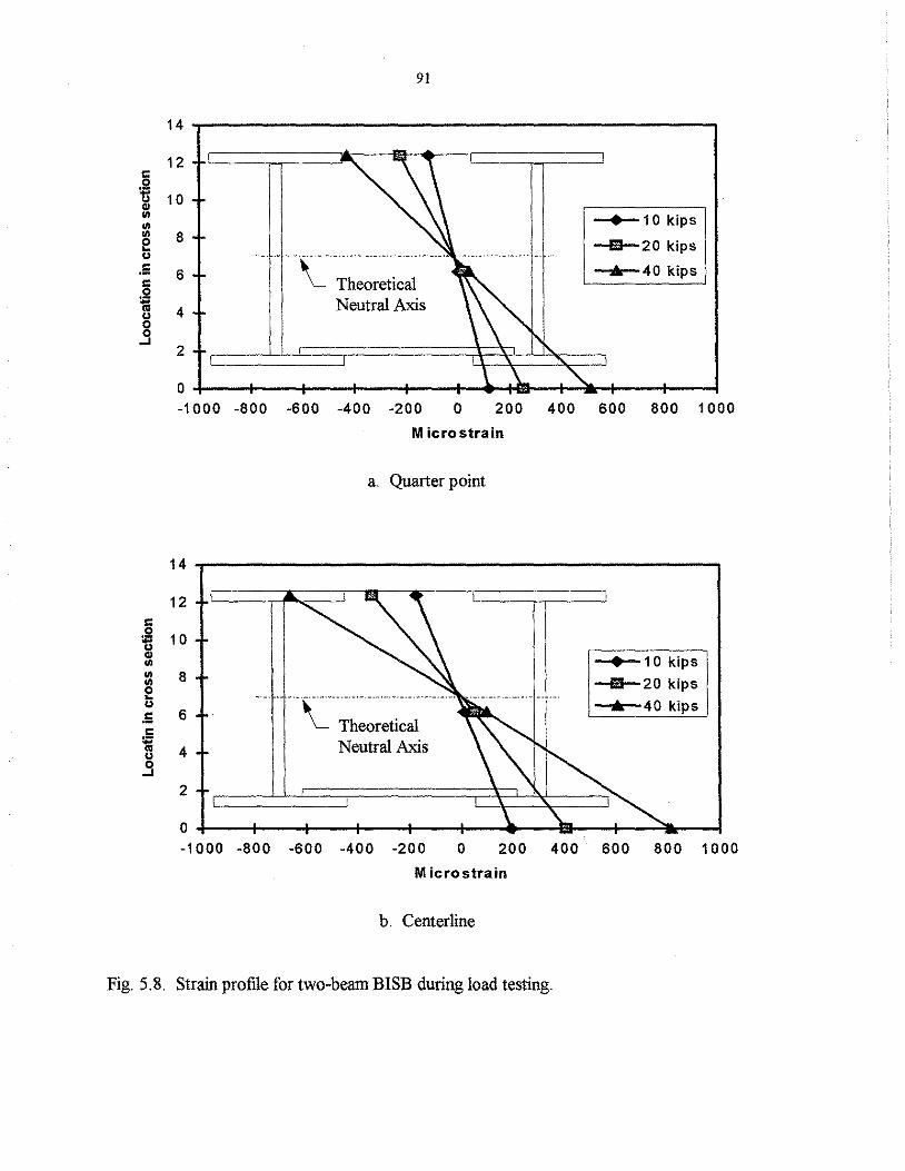
~ u .5
I
c
~ .. .. .. .. e u .5 c :; u .s
8
6
4
2
91
Theoretical Neutral Axis
-+-10 kips
-fD-20 kips
• 40 kips
0 +-~-t-~-+~--tr--~+-~+--+-+11!11---+---illir--!t--~+-~~ -1000 -800 -600 -400 -200 0 200 400 600 800 1000
14
12
10
8
6
4
2
M icrostrain
a. Quarter point
• 10 kips -lli'f-20 kips
• 40 kips
0 +-~-t-~-+~--11--~+-~-+-~-+~-e1-~1--~~~-1 -1000 -800 -600 -400 -200 0 200 400 600 800 1000
M icrostrain
b. Centerline
Fig. 5.8. Strain profile for two-beam BISB during load testing.
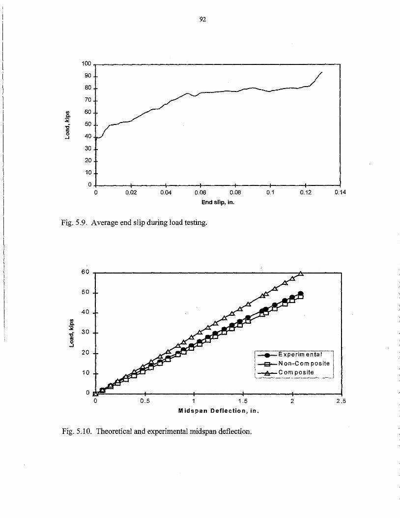
92
100
90
80
70
I/) Q.
60 :;:
50 .,; "' 0 40 ...
30
20
10
0 0 0.02 0.04 0.06 0.08 0.1 0.12
End slip, in.
Fig. 5.9. Average end slip during load testing.
60
50
40 I/) Q. :;;:
30 .,; "' 0 ...
20
10
0 0 0.5
1-e-Experim ental
-a-Non-Composite I --.e.-c om po site
1.5
Mids pan Deflection, in.
2
Fig. 5.10. Theoretical and experimental midspan deflection.
0.14
2.5
)
)

93
that the ASC will alleviate. Although minimal slip should occur throughout with
increased load, once the steel-concrete bond is broken, the load would be carried by the
ASC.
An attempt to quantify the amount of composite action is illustrated in Fig. 5.10.
In this figure, an experimental load versus deflection curve is compared to theoretical
composite action and non-composite action deflection curves. The non-composite graph
was determined by using the moment of inertia for the two steel beams only, and
assuming the concrete acted only as dead weight.
Similarly, the composite deflection curve was determined using the moment of
inertia of the entire section. The concrete area was modified into an equivalent steel area.
The theoretical load deflection curves were determined using the moment of inertia
values, the geometry of the test set-up, and basic load-deflection relationships.
In theory, the load versus deflection data for the composite beam should fall
between the theoretical values for complete composite action and non-composite action.
If the specimen behaved as expected, the structure should initially respond more like a
composite structure, as the concrete and the steel should have adequate bond. However,
as the load increases, the steel-concrete bond would weaken and the concrete in tension
would crack, causing the structure to behave increasingly as a non-composite structure.
As can be seen in Fig. 5.10, the structure initially responded as a composite beam.
At a load of approximately 22 kN ( 5 kips) per load point, the structure began to make the
transition to non-composite behavior, indicating that the bond between the steel and
concrete had been weakened. At a load of approximately 67 kN (15 kips), the beam acted
basically as a non-composite structure, with the concrete providing minimal composite
action.
5.2.2 Four-Beam Specimen
5.2.2.l Experimental Results
Service and ultimate load tests described in Chp 3 were performed on the four-beam
specimen described earlier. The goals of these tests were to: (1) determine the
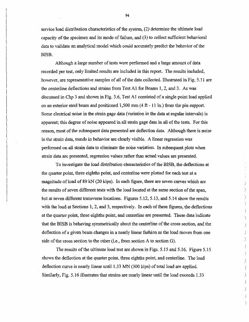
94
service load distribution characteristics of the system, (2) determine the ultimate load
capacity of the specimen and its mode of failure, and (3) to collect sufficient behavioral
data to validate an analytical model which could accurately predict the behavior of the
BISB.
Although a large number of tests were performed and a large amount of data
recorded per test, only limited results are included in this report. The results included,
however, are representative samples of all of the data collected. Illustrated in Fig. 5.11 are
the centerline deflections and strains from Test Al for Beams 1, 2, and 3. As was
disctissed in Chp 3 and shown in Fig. 3.6, Test Al consisted of a single point load applied
on an exterior steel beam and positioned 1,500 mm ( 4 ft - 11 in.) from the pin support.
Some electrical noise in the strain gage data (variation in the data at regular intervals) is
apparent; this degree of noise appeared in all strain gage data in all of the tests. For this
reason, most of the subsequent data presented are deflection data. Although there is noise
in the strain data, trends in behavior are clearly visible. A linear regression was
performed on all strain data to eliminate the noise variation. In subsequent plots when
strain data are presented, regression values rather than actual values are presented.
To investigate the load distribution characteristics of the BISB, the deflections at
the quarter point, three eighths point, and centerline were plotted for each test at a
magnitude of load of 89 kN (20 kips). In each figure, there are seven curves which are
the results of seven different tests with the load located at the same section of the span,
but at seven different transverse locations. Figures 5.12, 5.13, and 5.14 show the results
with the load at Sections 1, 2, and 3, respectively. In each of these figures, the deflections
at the quarter point, three eighths point, and centerline are presented. These data indicate
that the BISB is behaving symmetrically about the centerline of the cross section, and the
deflection of a given beam changes in a nearly linear fashion as the load moves from one
side of the cross section to the other (i.e., from section A to section G).
The results ofthe ultimate load test are shown in Figs. 5.15 and 5.16. Figure 5.15
shows the deflection at the quarter point, three eighths point, and centerline. The load
deflection curve is nearly linear until 1.33 MN (300 kips) of total load are applied.
Similarly, Fig. 5.16 illustrates that strains are nearly linear until the load exceeds 1.33
)
)
)
)
)
)

95
Top Flange Mid~ Web Bottom Ftange Deflection ~
00----------------------------~-o.15
,_ .....--=" ~~ -0.1
-~=- . -0.05.~
:.05 i 40
40 0.1
'----~---..L-----'-----'----~----,C..----' 0.15 "o 5 10 15 20 25 30 35 Load, kips
a. Strain and deflection in Beam 1
80----------------------------~-0.12
~ -0.08 ~--------- -0.04.!1
= 20 . ...:.:..'-"-~~ - -J _;~·..:·.;,-_--~-,.-_"'--_ :...<"::..·:··-:-_··::..·_··::..· ::::::~~~::::::,--= _========'-------i:.04 j ~ ~
0.08
""'o'--___ ,,_5----1"'0----+15 ____ 2"'0----='25---_.,,30-----,135°·12
Load, kips
b. Strain and deflection in Beam 2
... ,
5 lO 15 20 Load, kips
c. Strain and deflection in Beam 3
Fig. 5.11. Test Al Results: deflections and strains at centerline.
0.1
30 35
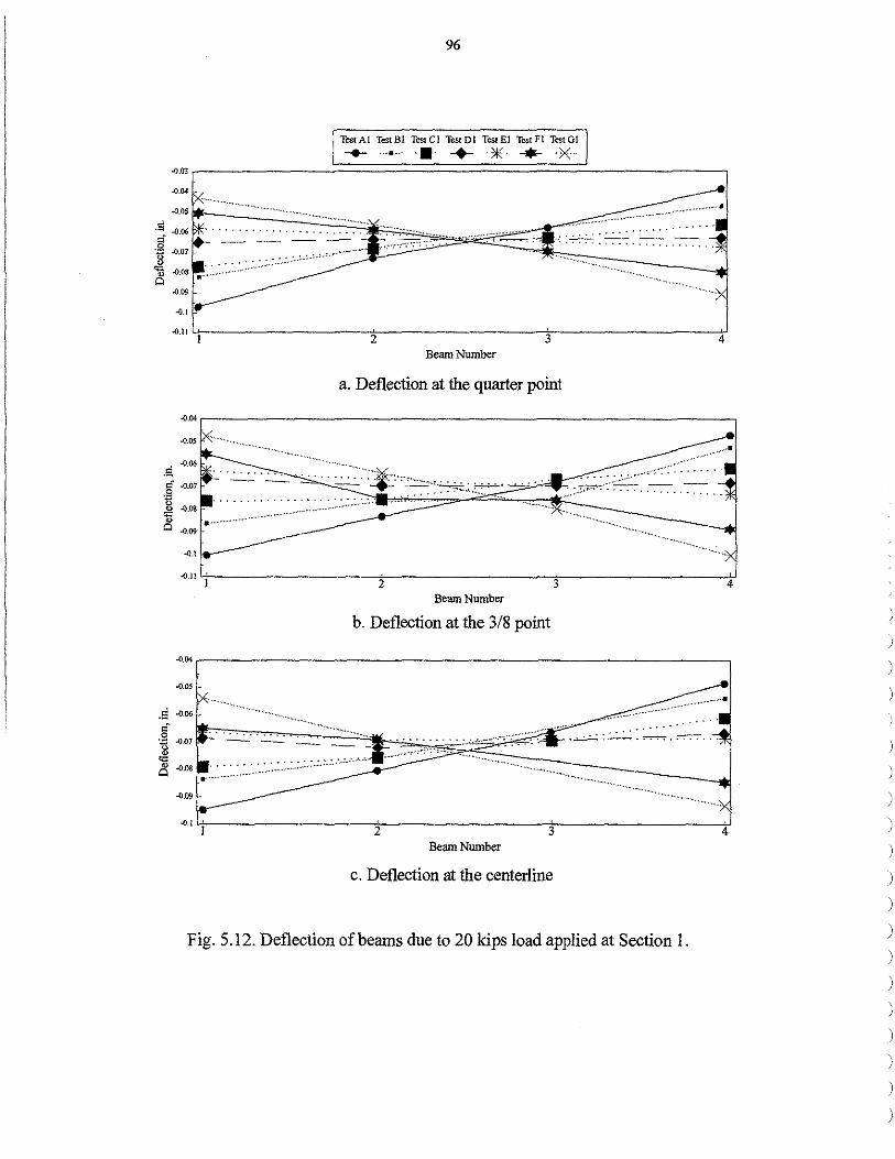
96
TestAI TestBl TestCl TestDl TcstEI TcstFI TestGI
--- . ·•· + •*• ..... >< -0.-03 ~--------=================---------~
.o.n c;------------<z----------30;-------------\-'4 Beam Number
a. Deflection at the quarter point
-0.<>4,--------------------------------~
-0.05
..o.n '+-----------kz----------30;------------+'4 Beam Number
b. Deflection at the 3/8 point
..... ~------------------------------~
..0.05
;.:...:-:....;..-:-:--;-:' .. -.-...
-0.09
... , '+-----------<z----------3!c----------_,_,4 Beam Number
c. Deflection at the centerline
Fig. 5.12. Deflection of beams due to 20 kips load applied at Section 1.
)
)
)
)
)
)
)
)
) . )
)
)
97
TestA2 TestB2 TestC2 TestD2 TestE2 TestF2 TestG2
...... ··• + •** x -0.%
-0.08
.5
j -0.I
-0.12
-0.14 l 2 3 4
Beam Number a. Deflection at the quarter point
-0.%~-----------------------------
-0.18 '-!-----------+2 _________ _,,3 __________ 4.,,
Beam Number
b. Deflection at the 3/8 point
-0.08------------------------------
-0.JS u_ _________ _,_2 _________ ..;.3 _________ _,_4
Beam Number
c. Deflection at the centerline
Fig. 5 .13. Deflection of beams due to 20 kips load applied at Section 2.
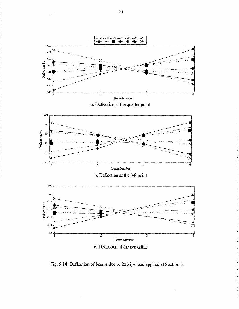
98
.5 cl' -0.1
.g ~ -0.11
8 -012
-0.!3
.Q14 [L ________ ___,_2 ________ ____,3 ________ __,J4
Beam Ntnnber
a. Deflection at the quarter point
-0.08----------------------------
-0.18 i 2 3 4 Beam Number
b. Deflection at the 3/8 point
-0.08
-0.J
.s -OJ2
cl' ·~ -0.14 . . . . . . "' Cl -0.16 )
-0.18 )
-02 ) 2 3 4
Beam Number
c. Deflection at the centerline
Fig. 5.14. Deflection of beams due to 20 kips load applied at Section 3.
)
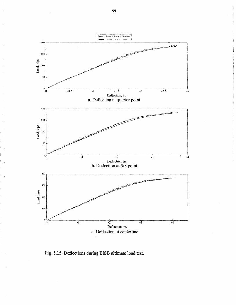
99
) Beam!~.~.~ s_~J Beam4 ! 400~~~~~~~~~~~--================'-~~~~~~~~~~~~
300
100
oo -0.5
100
-1
300
100
oo -1
-1 -1.5 -2 Deflection, in.
a Deflection at quarter point
-2 Deflection, in.
b. Deflection at 3/8 point
-2 Deflection, in.
c. Deflection at centerline
-3
Fig. 5.15. Deflections during BISB ultimate load test.
-2.5 -3
-3
-4

300
.e. ~ 200
] 100
300
JOO
-2',ooo -1,000
300 -
. & ~ 200
] 100
100
Top Flange Mid Web Bottom Flange
Microstrain
a Beam 1 strain at quarter point
0
. .
Microstrain 1,000
b. Beam 1 strain at centerline
Microstrain c. Beam 4 strain at centerline
Fig. 5 .16. Strains during ultimate load test.
:
2,000
' .
3,000
101
MN (300 kips). Both the deflection and strain curves become nonlinear at loads greater
than 1.33 MN (300 kips). The non-linear behavior is most likely the result of two
processes: yielding of the steel and the cracking of the tension concrete. Cracks became
visible between the concrete and the steel at 1.33 MN (300 kips). When the loading
apparatus was removed, additional cracks were visible around the holes through which
the loads were applied. The maximum load applied to the specimen was 1.65 MN (370
kips), which resulted in a maximum deflection of 103 mm (4.06 in.) at the centerline. At
this point, the bottom of the BISB specimen was in contact with the Dywidag bars used
to anchor the test apparatus to the tie-down floor. Continuation of the testing required the
disassembly of the entire loading apparatus and the repositioning of the BISB specimen.
For all practical purposes, the specimen failed; thus, the test was terminated.
5. 2. 2. 2 Comparison of Experimental and Analytical Results
Based on the results of the sensitivity studies discussed in Chp 4, a grillage model
of the four-beam BISB laboratory specimen was developed for comparison with
experimental data. The model used a transverse beam spacing of51 mm (2 in.). The
connection between the transverse beams and longitudinal beams was modeled as fixed
and the longitudinal beams were modeled as simply supported at the ends. The
transverse beams were modeled using the full contributory area of the concrete section 51
mm (2 in.) wide with a height of267 mm (10.5 in.) and the modulus of elasticity of
concrete. The longitudinal members were modeled using the transformed value of the
full contributory concrete width, 4.25 x 108 mm4 (1,020 in4) for the flexural moment. The
torsional moment of inertia used was 6.24 x 107 mm4 (150 in\ The longitudinal beams
used a modulus of elasticity of steel.
Figures 5.17 and 5 .18 show a comparison of experimental and theoretical
deflections (i.e., those obtained from the analytical model) for Tests Al and C3. These
tests were chosen to show the differences between the analytical and the experimental
results when the load is at an edge beam (Test Al) and on an interior beam (Test C3).

102
-0.03
I Experi:tal Grill~odel I
-0.04 --0.05 ~ -
.5 -0.06 d' .g .-0.07
al --13 -0.08 --Cl --0.09
--0.1
-0.11 2 3 4
Beam Number a. Deflection at the quarter point
-OM
-0.0S
-0.06 --.5 cf -0.07
.Q
8 -0.08
8 -0.09
~
-0.1
..0.li 2 3 4
Beam Number
b. Deflection at the 3/8 point
-0.04
-0.05
.5 -0.06 --d' -·~ -0.07 -0- --"" -8 -0.08 ----0.09 c--=--oo=-
--0.I 2 3 4
Beam Number
c. Deflection at the centerline
Fig. 5.17. Comparison of experimental and analytical results for BISB Test Al.

103
Fig. 5.18. Comparison of experimental and analytical results for BISB Test C3.
104
These figures show that the model gives results closer to experimental when the
load is placed on exterior beams. For all cases, the analytically predicted deflection is
within 15% of the experimental result.
5.3 Composite Beam Test Results
The composite specimen tests consisted of service and ultimate load tests of four
specimens. Both the details of the specimens and their instrumentation were presented in
Chp 2. These tests were performed to determine:(!) the service level strength of the
cross sections, (2) the degree of composite action between the concrete and steel for each
section under service level conditions, and (3) the ultimate strength and type of failure.
The results of the service level tests for Specimen 1 are illustrated in Fig. 5.19.
The strain at the centerline and the deflections at the quarter point, three eighths point,
and centerline are shown in Figs. 5. l 9a and 5 .19b, respectively. It can be seen that both
the strain and the deflection increased linearly with load. The strain across the section
depth is shown in Fig. 5. l 9c. The theoretical location for the neutral axis, assuming
"complete" composite behavior, was calculated and is also shown. Because the strain
across the section depth is nearly linear for each load level, and also because the
experimental and theoretical neutral axes are nearly the same, it is assumed that complete
composite action existed during the service level tests. Based on these sets of data, it is
concluded that the ASC used in the specimen was effective in creating composite action
between the concrete and the steel.
As noted in Chp 2, Specimens 2 and 3 were the same. Some unexplainable test
results were observed in the testing of Specimen 2; thus, Specimen 3 was fabricated to be
identical to Specimen 2 and tested to provide additional data. Figure 5 .20 shows a plot of
both deflections and strains for Specimens 2. From these graphs, it appears that the
longitudinal flexural stiffness of Specimen 2 decreased after 44.5 kN (I 0 kips) ofload
were applied.
However, this change in stiffness is suspicious to the researchers for a couple of
reasons. In general, a change in longitudinal flexural stiffiless could be caused by one of

20
~
~ 15
~ 10
-'400
.E 20
§ ·~ IS ~
i2 e Q JO .s .g ~
105
-200 Microstrain
a. Strain at centerline
-0.1 -0.2 -0.3 Deflection, in.
b. Service test deflections
beoretical - Neutral Axis
Microstrain
c. Strain throughout cross section depth
Fig. 5.19. Specimen 1 service test results.
400
-0.4
15 kips
Concrete
rmbti'e<1 ~
Tcp-wcl>
Mid~wci> Bo~web
Bonoit'iange
+
Quaner Point
1/st;"1n1 ~
Centerline
+
20 kips
-0.5
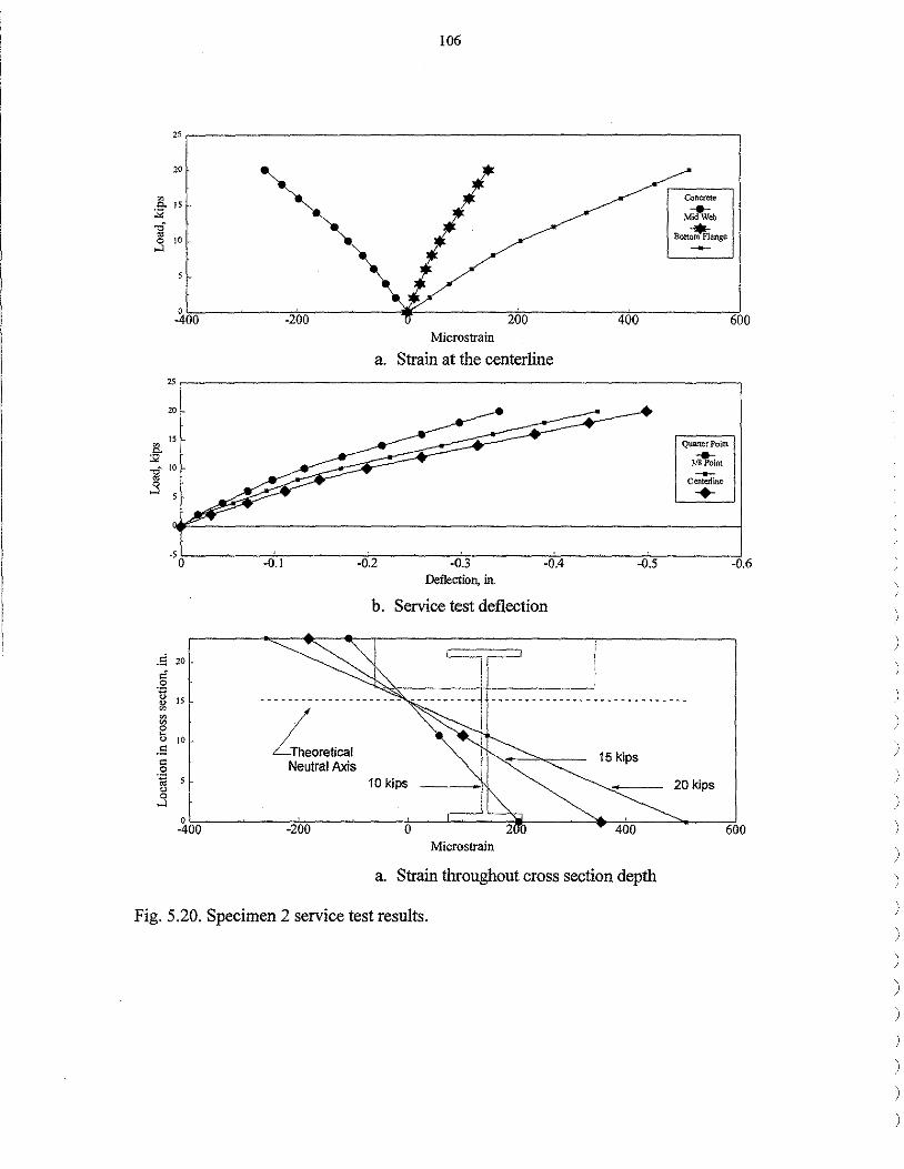
106
20
400 -200 200 Microstrain
a. Strain at the centerline
20
" .9. .¥
-g" !O
.s 5
400
C.Oncrete
Mi1w°eb Bott~ange ~
Quarter Point
~int ~
Centerline .....
600
"'o,,_ ___ ~-o"°".,..1----_.,;o.""2----...,_0,.,.3,-------0"".4.,._-~---0~.s-----;_o.6
.E 20 -
.~ g IS ~
~ " iO .s " j
Loretical Neutral Axis
Deflection, in.
b. Service test deflection
15 kips
10 kips
Microstrain
a. Strain throughout cross section depth
Fig. 5.20. Specimen 2 service test results.
20 kips
600
)
)
)
)
)
)
)
)
)
)

107
two things: inelastic behavior or loss of composite action. Inelastic behavior is unlikely
in this specimen because the strains in both the concrete and steel were within their
respective elastic ranges when the behavior changed. Additionally, inelastic behavior
causes permanent deformation of the material. No permanent deformation occurred in
the specimen, and the change was abrupt and occured in several service load tests of the
specimen and the ultimate load test. The second explanation, loss of composite action,
would correspond to a change in the location of the neutral axis; no change in the neutral
axis was observed.
The only logical explanation for the behavior observed is an error in the
measurement of the applied load. Such an error would explain strain and deflection
curves; it is also likely that an electrical or mechanical error would repeat in each test, as
was observed. Since the results of Specimen 2 are unexplainable, they are not used for
comparison in the following sections. However, a comparison of strains and deflections
for Specimens 2 and 3 were made and are illustrated in Fig. 5 .21. Both the strain and
deflection curves are similar up to the load of 44.S kN (10 kips). The location of the
neutral axis is the same for both specimens for a 89 kN (20 kips) load. This provides
further verification that the error in Specimen 2 data was the result of an error in the
measurement of the applied load.
The service test results for Specimens 3 and 4 are shown in Figs. 5.22. and 5.23,
respectively. Both of these specimens exhibit linear behavior based on both deflection
and strain data. Because similar behavior is inferred by both the strain and the deflection
data, only deflection data are present in the rest of this section. As with Specimen 1, the
strain across the section depth was nearly linear and the experimental location of the
neutral axis agreed closely with the theoretical location. This indicated that both the ASC
and the shear stud connector created composite action between the concrete slab and the
steel beam.
Centerline deflections for Specimens 1, 3, and 4 are compared in Fig. 5.24. As
shown in Fig 5 .24a., the specimens have different longitudinal flexural stiffnesses,
Specimen 4 having the greatest and Specimen I having the least. When the deflection
data are modified for the variation in longitudinal flexural stiffnesses (see Fig 5.24b.), the

20
a IS :!<
110 _,
20
.e. IS ... -g 3 10
.5 20
-~ g JS ~
~ - JO
.5
.§ 1<! s " 0 _,
-200
-200
108
200 Microstrain
a. Strain at the centerline
400
Concrete Specimen 2
Bottom Fla-;;:specimen 2
concretetimen 3 ~
bottom flange specimen 3
+
600
Quarter Point Specimen 2
Cente!li;1pecimen 2 ~
Quarter Point Specimen 3
Centerli~imen 3
+
-0.1 -0.2 -0.3 -0.4 -0.5 -0.6
Leoretical Neutral Axis
Deflection, in
b. Service test deflection
1 ~r I - - - -- - - - - - - - - __ ( l - - - - - - - - -- - - - - - - - - -- - - - h - - -
0 Microstrain
a. Strain throughout cross section depth
600
Fig. 5.21. Comparison of service test results of Specimens 2 and 3.
)
)
)
)
)
)
)
)
)
)
)
)
)

20
20
~ 15
-g 3 JO
.5 20
§ -~ 15 ~
~ <.) 10 .s " 0 -~ s
.s
-0.1
109
Micro strain a. Strain at the centerline
-0.2 Deflection, in.
b. Service test deflections
ze~re!l~I-- - -----
Neutral Axis 10 kips
Micros train
-0.3
15 kips
c. Strain throughout cross section depth
Fig. 5.22. Specimen 3 service test results.
Concrete
--Top-web
M%-eb ~
Bottom-web
Botto~ange
*
~
Centerline
+
-0.4

110
20
~00 -200
Microstrain a. Strain at the centerline
-0.0001 -0.00015 -0.0002 -0.00025 Deflection, in.
b. Service test deflections
.s "
" ·£ 20
" ~
Microstrain
400
-0.0003
15 kips
Concrete ..... Top-web
M~eb ~
Bottom-web
Botto~ange ..
Quarter Point
3i8t;int ~
Centerline
-+-
-0.00035
20 kips
c. Strain throughout the cross section depth
Fig. 5.23. Specimen 4 service test results.
)
)
)
)
)
)
)
)
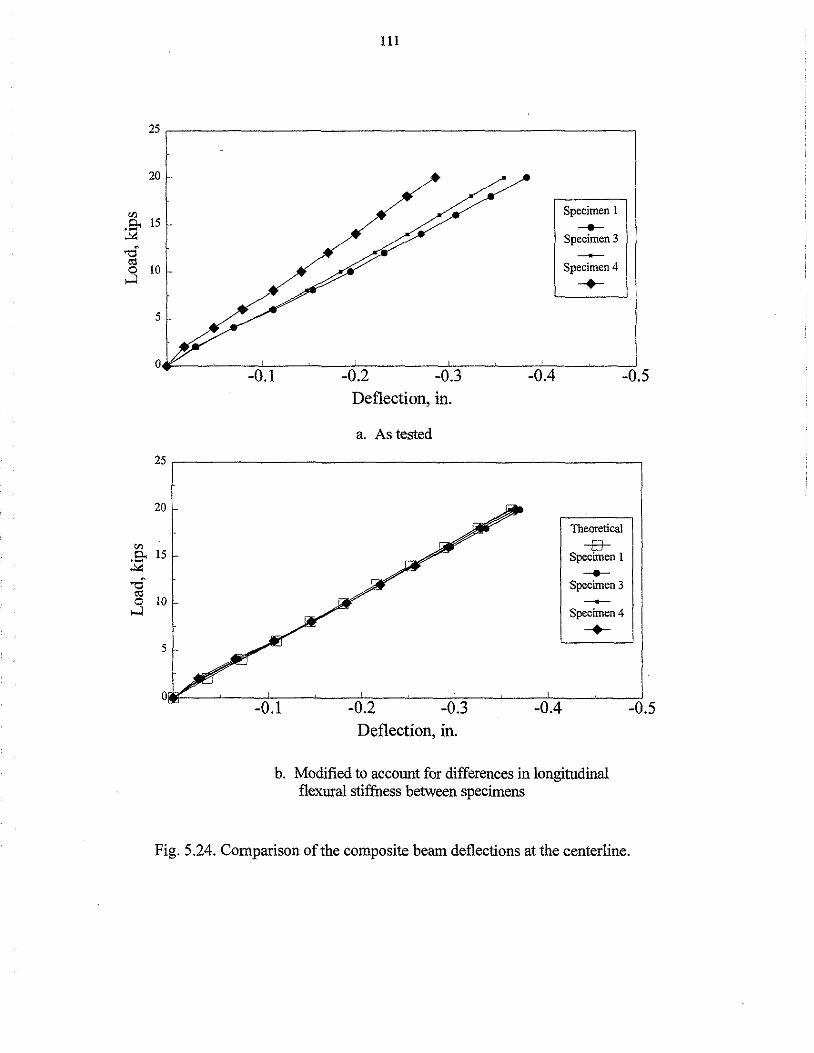
"' .8' ,.,,. "O"
o:I 0
,...:i
"" .a. ..::.: "O" o:I 0
,...:i
25
20
15
10
5
0
25
20
15
lO
5
0
111
Deflection, in.
a. As tested
Deflection, in.
-0.4
Specimen I __.__
Specimen 3
Specimen 4
-+--
-0.5
Theoretical
-a-Specimen I __.__ Specimen 3
Specimen4
-+--
-0.4 -0.5
b. Modified to account for differences in longitudinal flexural stiffness between specimens
Fig. 5.24. Comparison of the composite beam deflections at the centerline.
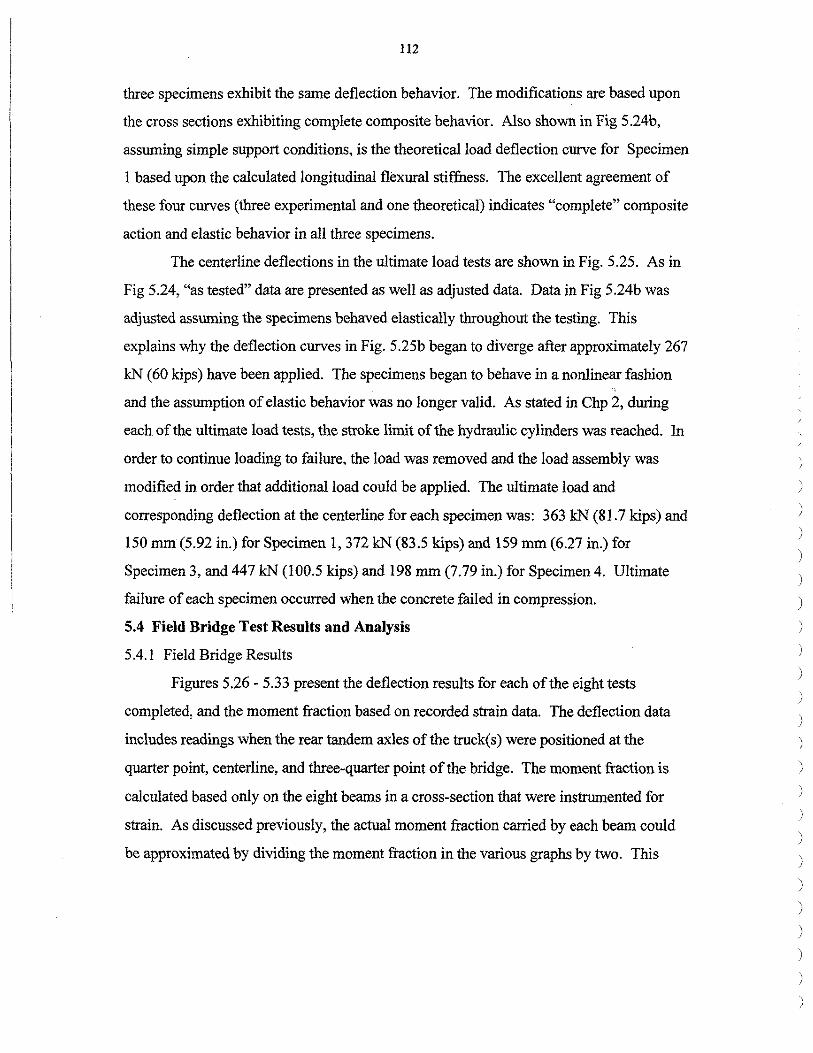
112
three specimens exhibit the same deflection behavior. The modifications are based upon
the cross sections exhibiting complete composite behavior. Also shown in Fig 5.24b,
assuming simple support conditions, is the theoretical load deflection curve for Specimen
1 based upon the calculated longitudinal flexural stiffness. The excellent agreement of
these four curves (three experimental and one theoretical) indicates "complete" composite
action and elastic behavior in all three specimens.
The centerline deflections in the ultimate load tests are shown in Fig. 5.25. As in
Fig 5.24, "as tested" data are presented as well as adjusted data. Data in Fig 5.24b was
adjusted assuming the specimens behaved elastically throughout the testing. This
explains why the deflection curves in Fig. 5.25b began to diverge after approximately 267
kN (60 kips) have been applied. The specimens began to behave in a nonlinear fashion
and the assumption of elastic behavior was no longer valid. As stated in Chp 2, during
each of the ultimate load tests, the stroke limit of the hydraulic cylinders was reached. In
order to continue loading to failure, the load was removed and the load assembly was
modified in order that additional load could be applied. The ultimate load and
corresponding deflection at the centerline for each specimen was: 363 kN (81.7 kips) and
150 mm (5.92 in.) for Specimen 1, 372 kN (83.5 kips) and 159 mm (6.27 in.) for
Specimen 3, and 447 kN (100.5 kips) and 198 mm (7.79 in.) for Specimen 4. Ultimate
failure of each specimen occurred when the concrete failed in compression.
5.4 Field Bridge Test Results and Analysis
5.4.1 Field Bridge Results
Figures 5.26 - 5.33 present the deflection results for each of the eight tests
completed, and the moment fraction based on recorded strain data. The deflection data
includes readings when the rear tandem axles of the truck( s) were positioned at the
quarter point, centerline, and three-quarter point of the bridge. The moment fraction is
calculated based only on the eight beams in a cross-section that were instrumented for
strain. As discussed previously, the actual moment fraction carried by each beam could
be approximated by dividing the moment fraction in the various graphs by two. This
)
)
)
)
)
)
)
)
)
)
)
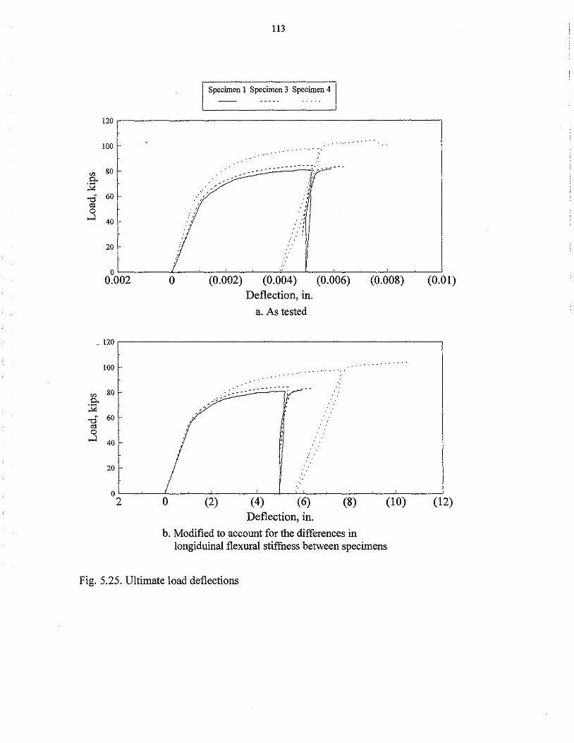
120
100
"' 80 i:i.. ·-,;..:
..cf 60 o:! 0
....l 40
20
0 0.002
120
100
"' 80
i:i.. ;g ..cf 60 o:! 0
....l 40
20
0 2
.·,
0
0
113
Specimen I Specimen 3 Specimen 4
..........
-.;.:..:-::.:-=----t•, ---... ·' ·' . •' . , ,
' , . ·•' ·' " ·' . : ~
(0.002) (0.004) (0.006)
(2)
Deflection, in.
a. As tested
. . . . . . . . . . -.......... .
(4) (6)
Deflection, in.
.. ''
(8)
(0.008)
(10)
b. Modified to account for the differences in longiduinal flexural stiffness between specimens
Fig. 5.25. Ultimate load deflections
(0.01)
(12)
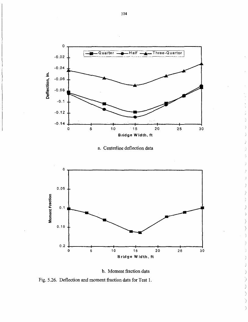
114
0
I _Quarter _._Half......,_ Three-Quarter I -0.02
-0.04
.5 c -0.06
:8 ... -0.08 Cl
'ii c -0.1
-0.12
-0.14 0 5 10 15
Bridge Width, ft
a. Centerline deflection data
0.05
c 0 ., " I! IL 0.1 -c .. e 0 :;;
0.15
0 5 10 15
Bridge Width, ft
b. Moment fraction data
Fig. 5.26. Deflection and moment fraction data for Test 1.
20 25
20 25
30
)
30
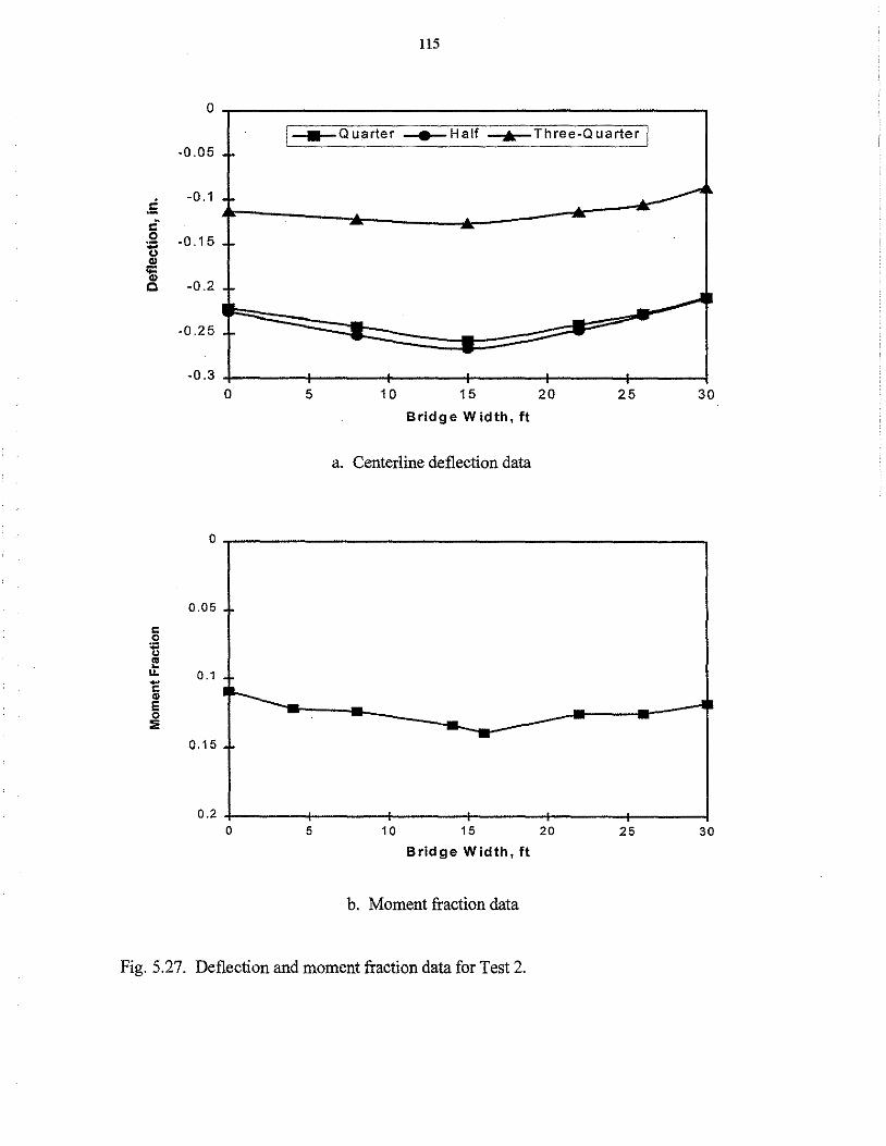
.5 c 0
~ 't c
115
[-Quarter -e-Half _._Three-Quarter j
-0.05 ·-
-0.1 ·- .___......~ t----.-__ _._ __ -.tc--___
-0.15 ·-
-0.2 ·---1 I
-0 . 2 5, __ ~=:::::::::::::::::::::::::::...,
-0.3 +--------+--------!--------+-------~.--------+-------~ 0 5
0.05 .•
0.1 •
10 15
Bridge Width, ft
a. Centerline deflection data
~---m--:---------...---0.15 .•
20 25 30
0.2 +--------+-.------~-------+-.------~.--------+-------~ 0 5 10 15 20 25 30
Bridge Width, ft
b. Moment fraction data
Fig. 5.27. Deflection and moment fraction data for Test 2.
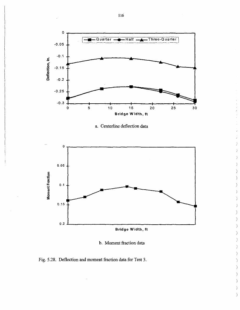
116
0
I-Quarter -e-Half __._Three-Quarter\ -0.05
.5 -0.1
c ~ -0:15 '-' ~ .. c -0.2
-0.25
-0.3 0 5 10 15 20 25
Bridge Width, ft
a. Centerline deflection data
0.05
c 0 .. " I?! .... 0.1 ... c
" E 0 ::;;
0.15
Bridge Width, ft
b. Moment fraction data
Fig. 5.28. Deflection and moment fraction data for Test 3.
30
)
)
)
)
)
)
)
)
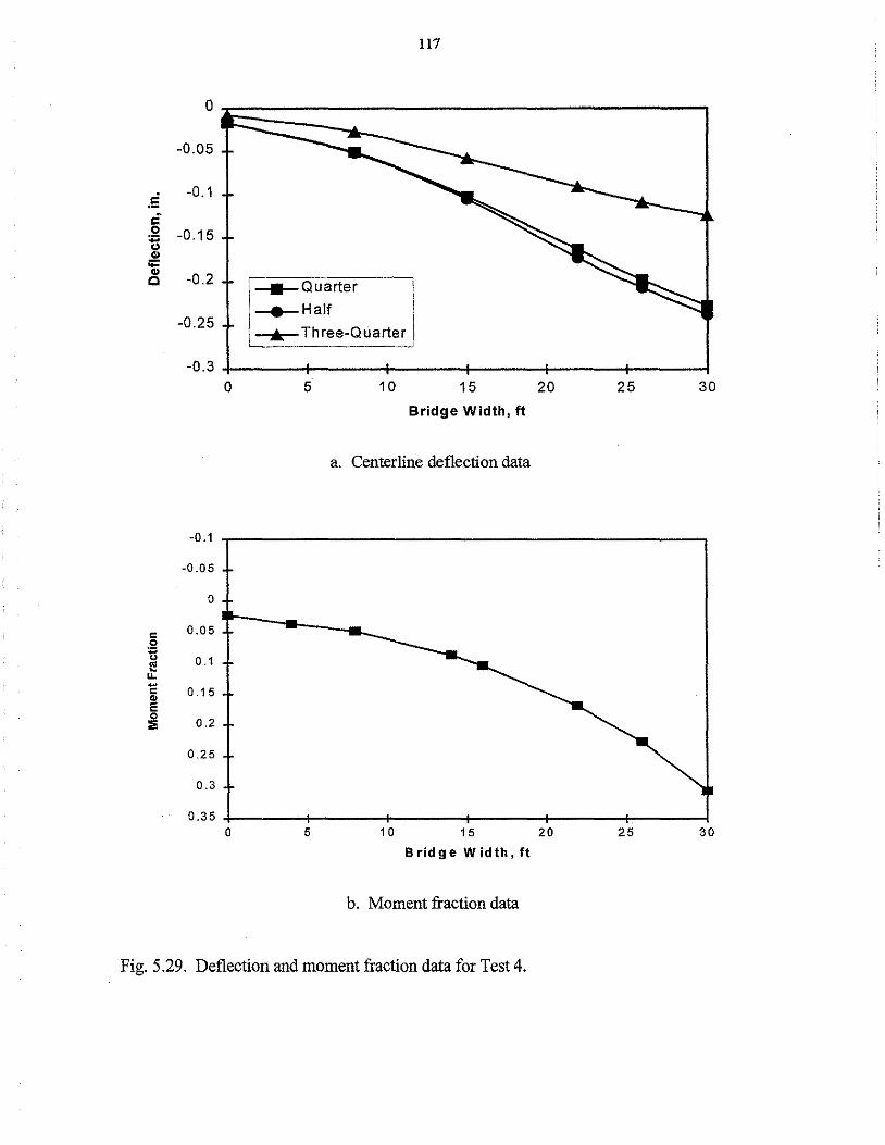
0
-0.05
.5 -0.1
c 0 -0.15 ~ .. 't -0.2 c
-0.25
-0.3
-0.1
-0.05
0
" 0.05
0 :;:: u 0.1 f! IL - 0 .15 " " E 0
0.2 ::;;
0.25
0.3
0.35
0
0
117
-e-Half ! ~--Quarter i
.......,__Three-Quarter I
5
5
10 15
Bridge Width, ft
a. Centerline deflection data
10 15
Bridge Width, ft
b. Moment fraction data
Fig. 5.29. Deflection and moment fraction data for Test 4.
20 25 30
20 25 30
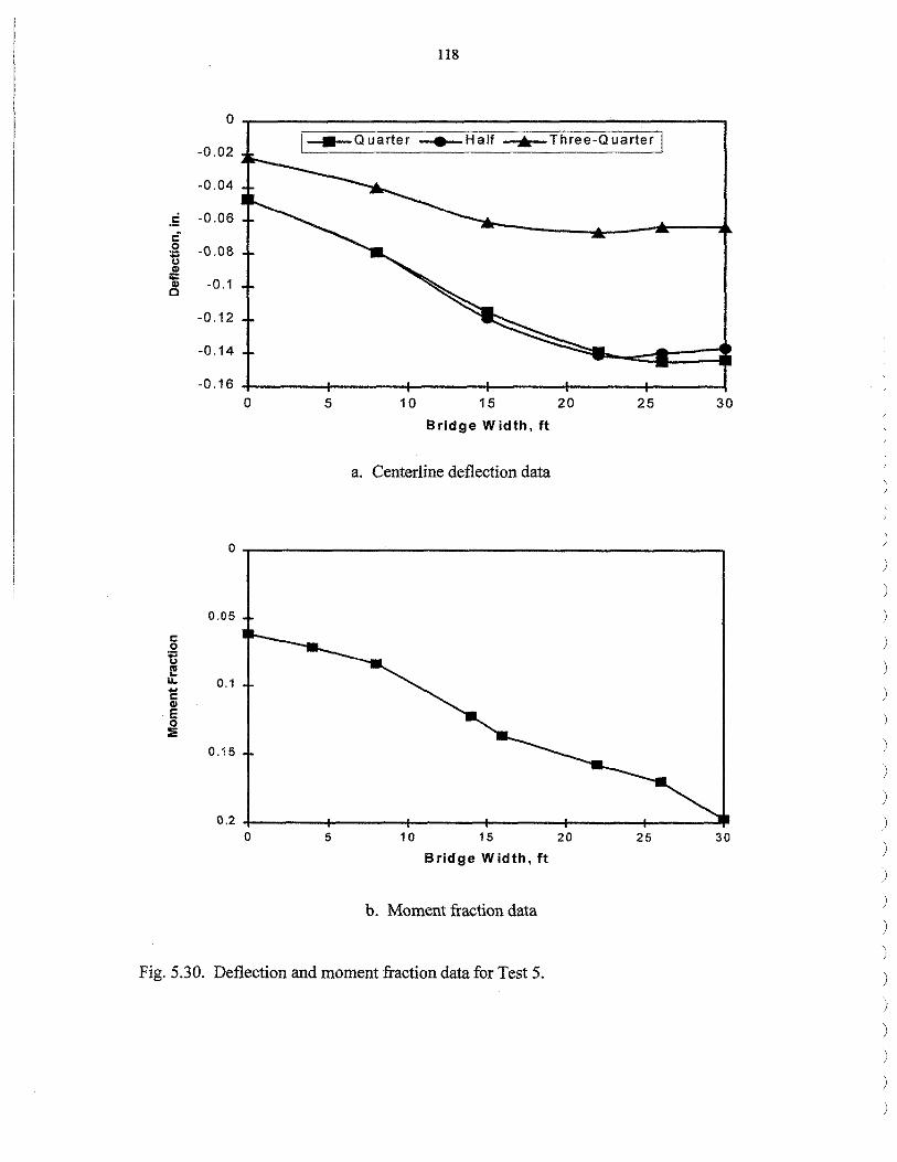
118
0
-0.02 1---0 uarter -.-Half _,.__Three-Quarter I
-0.04
.E -0.06 .: 0 -0.08 "" " .. ;;:
-0.1 " c
-0.12
-0.14
-0 .16
0 5 10 15 20 25 30
Bridge Width, ft
a. Centerline deflection data
.. :r c
~ l! u. 0.1 -c .. E 0 :;;
0.15
0.2 +---------------------+----""' 0 5 10 15 20 25 30
Bridge Width, ft
b. Moment fraction data
Fig. 5.30. Deflection and moment fraction data for Test 5.
)
)
)
)
)
)
)
)
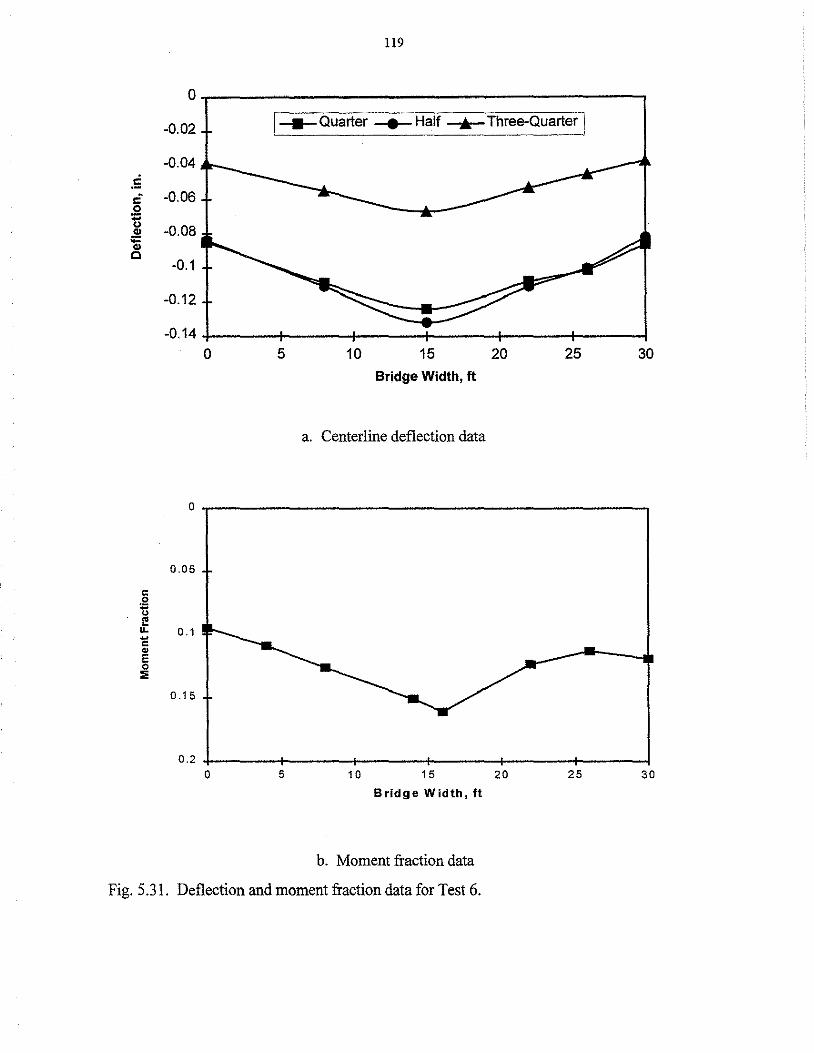
119
0
-0.02 I-Quarter -e- Half __.__Three-Quarter I
-0.04 .5 c -0.06 0
:n -0.08 "' ~ c
-0.1
-0.12
-0.14
0.05
c
~ f u. 0.1 -c .. E 0
::;;
0.15
0 5
0 5
10 15
Bridge Width, ft
a. Centerline deflection data
10 15
Bridge Width, ft
b. Moment fraction data
Fig. 5.31. Deflection and moment fraction data for Test 6.
20 25
20 25
30
30
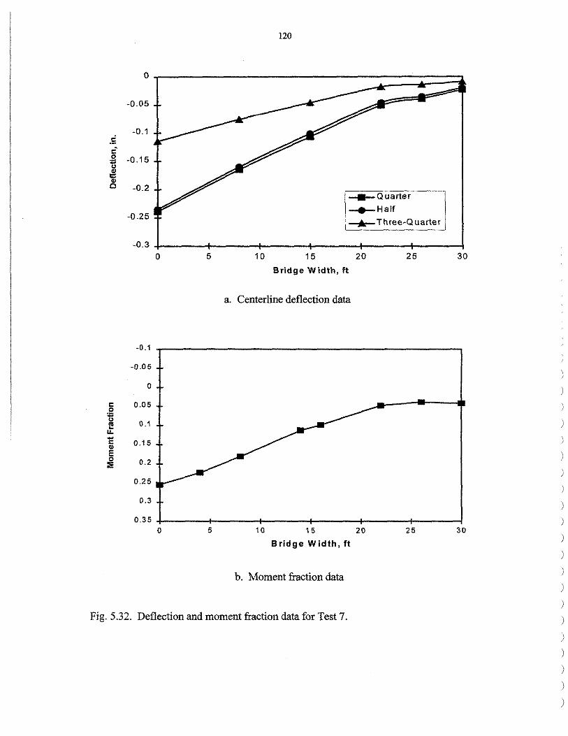
120
0
-0.05
-0.1 .5 r::." 0 -0.15 "' "' .. i5 c -0.2
-0.25
1-Quarter I _._Half
I.._.._ Three-Quarter I -0.3
0 5 10 15 20 25
Bridge Width, ft
a. Centerline deflection data
;·.:i c 0.05 ~ "' 0.1 f! u. ..., c 0.15 .. E 0 0.2 :;;
0.25
0.3
0.35 0 5 10 15 20 25
Bridge Width, ft
b. Moment fraction data
Fig. 5.32. Deflection and moment fraction data for Test 7.
30
30
)
)
)
)
)
)
)
)
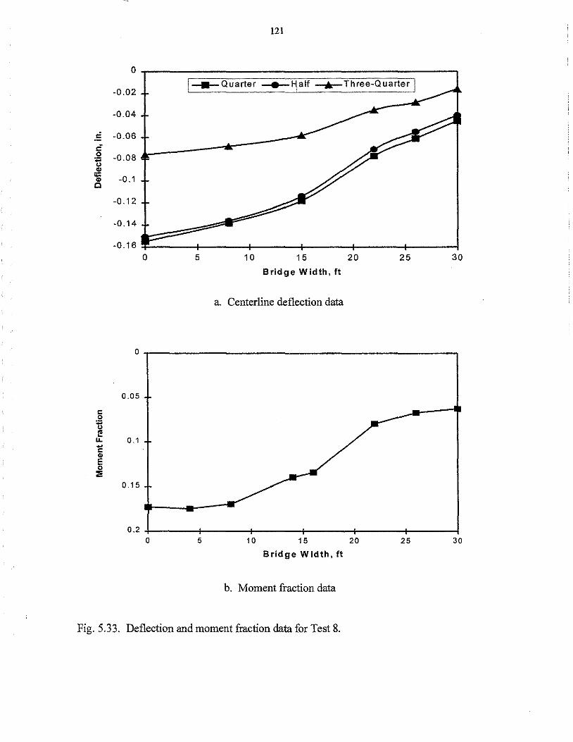
0
-0.02
-0.04
.5 -0.06 c 0 -0.08 = " ..
'Si c -0.1
-0.12
-0.14
-0.16 0
0.05
c 0 t; E LL 0.1 -c
"' E 0 :il
0.15
0
121
l-11-0uarter -e--H,alf -.-Three-Quarter I
5
5
10 15
Bridge Width, ft
a. Centerline deflection data
10 15
Bridge Width, ft
b. Moment fraction data
20 25
20 25
Fig. 5.33. Deflection and moment fraction data for Test 8.
30
30

122
would be true, assuming the strain in non-instrumented beams would be equal to an
average of the strains in the adjacent instrumented beams.
Overall, the deflection data indicated that the BISB was a very stiff structure both
longitudinally and transversely. With a total load of approximately 445 kN (100 kips)
(Test 2), the maximum deflection of the bridge was only 6 mm (114 in.). Longitudinally,
there was very little difference in deflections when the truck was positioned at the quarter
point or at the centerline. The maximum deflections varied by only 0.3 mm (0.01 in.).
The large difference in the deflections when the trucks were at the three-quarter span can
be attributed to the fact that the front axle of the truck was off of the bridge. Because
approximately half of the weight of the trucks was positioned on the bridge, it would be
assumed that the deflections would likewise be approximately half. This is true as can be
seen in Fig. 5 .26a.
Transversely, the load was very effectively distributed throughout the width of the
bridge. As can be seen in Fig. 5 .26b, with the load centered on the width of the bridge,
the exterior beams still resisted a significant portion of the load. With 16 beams in the
bridge, an even load distribution would result in 6.25% of the total load being carried by
each beam. As explained earlier, the moment fraction of 0.1 for the exterior beams in
Fig. 5.26b represents 0.05 (5%) of the total load. This demonstrates that the concrete
between the steel beams adequately transferred the service loads to adjacent beams.
Symmetry of the field bridge was checked by comparing the deflections at
midspan for Tests 4 and 7, and Tests 5 and 8. For Tests 4 and 7, the truck was positioned
on the outermost lane of the bridge, on opposite sides. Although test vehicle 1 was used
for Test 4 and test vehicle 2 for Test 7, the weights of the two trucks were similar; thus, a
graph of the two tests should produce symmetrical results. As can be seen in Fig. 5.34a,
the deflections at the center of the bridge were within 5% of each other which can be
attributed to the different truck weights; thus, the bridge behaves symmetrically.
Additionally, Fig. 5.34b illustrates with the trucks at midspan - one positioned in lane 2
and one positioned in lane 4 - deflections at the center are within 5%, thereby confirming
the symmetry in the bridge.
)

.5 c 0
"' (.)
" ;::
" c
0
-0.05
-0 .1
-0.15
-0.2
-0.25
-0.3 0
0
-0.02
-0.04
.5 -0.06
c 0 -0.08 11 " 'ii -0.1 c
-0.12
-0.14
-0.16 0
123
-+--Truck at M idspan--Lane 1
- Truck at M idspan--Lane 5
5 10 15
·Bridge Width, ft
a. Truck in lanes 1and5
I-• Truck at Midspan--Lane 21 l=-Truck at Midspan--Lane 4 I
5 10 15
Bridge Width, ft
b. Truck in lanes 2 and 4
20
20
Fig. 5 .34 Symmetry determination on field bridge.
25 30
25 30
124
5.4.2 Comparison of Experimental and Analytical Results
A grillage model (sec Fig. 5.35) of the field BISB was developed to allow
comparison of analytical and experimental data. The analytical model was developed
based on principles presented earlier in Chp 4 and with consideration to the results of the
sensitivity study presented in the same chapter.
The moment of inertia was calculated based on the moment of inertia of the steel
beam plus the moment of inertia of the contributary area of the concrete, resulting in
moment of inertia of3.50 x 108 mm4 (840 in4) and 4.25 x 108 mm4 (1020 in4
) for the
exterior and interior beams, respectively. The modulus of elasticity and Poisson's ratio
were assumed to be 200 GPa (29,000 ksi) and 0.3 respectively, which are common
properties of structural steel.
The transverse beams were connected to the longitudinal beams by links
(BEAM44). All data provided herein used a fixed connection for the link member. The
links were spaced at 152 mm (6 in.) longitudinally along the entire bridge (see Fig. 5.35).
The moment of inertia of the links was based on the contributary area of concrete
between the steel beams, and was calculated at 175 x 108 mm4 (420 in\ The modulus of
elasticity was input as 29 GPa ( 4200 ksi), an approximation based on the 28-day concrete
compressive strength of the composite beam tested in the laboratory. Poisson's ratio was
assumed to be 0.15.
For each truck on the bridge, six concentrated loads were placed on the finite
element model to represent the six truck wheel loads. Support conditions of the
longitudinal beams were then modeled assuming both pinned and fixed rotational
restraint.
Figures 5.36-5.42 present the results of the theoretical analysis, along with the
experimental results for each test, with the truck(s) at midspan longitudinally. Test 6 has
been excluded since it was a repeat of Test 1, and the data were very similar.
As described earlier, the dowels connecting the superstructure and the abutment
provide a certain amount of longitudinal beam end fixity. It can be seen by the results in
Figs. 5.36-5.42 that this connection more closely resembles a fixed condition than a
)
)
)
)

100 6 in
l
I
I
I SPA@
r, . =50ft A -
I
I I l i -I
I i
I t
14-_____ 15 SPA@2 ft= 30 ft
Fig. 5.35. Field bridge grillage analogy.
125
'
- F d d 1xe orp1nne end condition
~
'\
'-
'\
~Con crete links fixed ends
AM44) with (BE
'\
In w
terior beams 12x77 (BEAM4)
Exterior beams C8x30 (BEAM4)
\ .1 ~ F:xed or pinned
end condition

126
0
'~-- . . ... --. . J::.. - --- ---1::... __ A·. - . -. . - . --. .c -. - ···J::..---- --0.1
.E - - 0 - • Theoretical: Pin
.c
• Experimental
c 0 -0.2 :s Cl>
~ c - -~ - - Theo retie a I: Fix
l. - . . ---- - .c· -. --.. c· -- -. c. - - . .. ..... ·-----c--- - --
' . '
-0.3
-0.4 0 5 15 20 25 30
Bridge Width, ft
Fig. 5.36. Comparison of theoretical and experimental deflections at midspan:
.E c 0
~ "' ~
Test 1.
-0.1 c
. :.- - .. - - - .. - -1::..- - - .. - - - - A- - - - - - . - .. A·. - . - A . . - . ':. -0.2t-·----...__ ______ _., _ __.I-'-_, -0.3 •
-0.4 .c
-0.5 .c
-0.6 .
-0 .7 1_, ••• - •• - - •• ·C - ..., - . - .... C·. - - - C ... .. l - -- ...... - . -"'-'- --
0 5 10 15 20 25 30
Bridge Width. ft
Fig. 5.37. Comparison of theoretical and experimental deflections at midspan: Test 2.
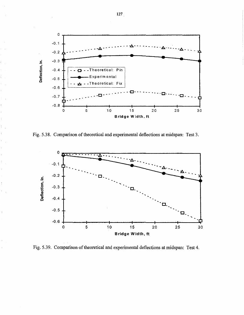
.5 c
I
127
-0 .1 - -·---·-.,0.--------- £:.. .
- - ... -1::. - - - . . - - . - -,o.. - - - ., ' -0. 2 ' !I. - - • - - -
-0.3
-0.4 .c. - - o - -Theoretical: Pin
-0.5 L --•~-Experimental
- - 71::s:: - -Theoretical: Fix -0 .6 . L.. L... _________ ___,
- - .. - o- - - - - - . - - . CJ -0. 7 . '" - - . - •. - -CJ - - • . . • - . - -CJ - - - - t J
I]- .. -0 .8 ..1-___ _. ____ .._ ___ _.. _____ ,__ ___ _.._ ___ --1
0 5 10 15 20 25 30
Bridge Width, ft
Fig. 5.38. Comparison of theoretical and experimental deflections at midspan: Test 3.
0 .... - .......... - - ... .. ..... -.. . . ·J::. . •. -0.1 .. . . . ..
. 5 -0.2 • CJ •
c ' 0 -0.3 • CJ. ;;
" Cl>
'ii -0.4 Q • CJ • .
-0.5 . t:J. '
-0.6 0 5 10 15 20 25 30
Bridge Width, ft
Fig. 5.39. Comparison of theoretical and experimental deflections at midspan: Test 4.

0 ... - - a --.
-0 .1 .c
.E -0.2 c -~- . . . . . 0 n Cl)
-0.3 rs; .c c
-0.4 I· - 0 -·"I • 1- - '°" -
-0.5 0
128
--. - ·i::i..- - -. -- . . . ·i::i..- •. .. -
. . . . . t:I. . . . .
• Theoretical:
Experim en ta I
- Theoretical:
. .
5 10
. . . . . Pin t:I. . . . . Fix
.
15
Bridge Width, ft
.. -•,/',.. -- --./\ -- - --
. . . . ·c •••.• •CJ . -. -- J . .
20 25 30
Fig. 5.40. Comparison of theoretical and experimental deflections at midspan: Test 5.
0
-0.1
-0.2 .5 c 0 -0.3 ""' " Cl)
rs; c -0.4
.c· ·0.5
-0.6 0 5 10
.CJ"
15
Bridge Width, ft
20
"'°'.--··
--. -o· -
25 30
Fig. 5.41. Comparison of theoretical and experimental deflections at midspan: Test 7.
. )
)
)
)
)
)
)
)

129
0
-0.1
1::..--· --,o.----------A· .. ---
. -- .. .. .. .. . - ·-·A··· ,. -- --- -- -
.5 -0.2 . •• I l -. - • CJ" c
0
"" " ., -0.3
~ Q
-Theoretical: Pin -. -- - 0 - • CJ"
• Experimental --. . . . - - Theoretical: Fix . . - - -J::r - . . . a· . . . . . -0 .4 . . . - . . . o· .
- . - .. - .. -. --0.5 . . . .
0 5 10 15 20 25 30
Bridge Width, ft
Fig. 5.42 Comparison of theoretical and experimental deflections at midspan: Test 8.
0
0.02
0 .04 • -c 0
0 .06 • -n I! u. 0.08 • -'!: ., E 0 .1 • -0 ::;; . ,_
0 .12
0 .14 .. 0 .16
0
- - -<> - -Theroetical: Fix
• Experim en ta I
-~ ----<>' ._,. - - - - - - Q- ·<r - . -
. . 5 10 15 20
Bridge Width, ft
•> .- . :..... . ..---
25 30
Fig. 5.43. Comparison of theoretical and experimental moment fractions at midspan: Test 2, truck at midspan.
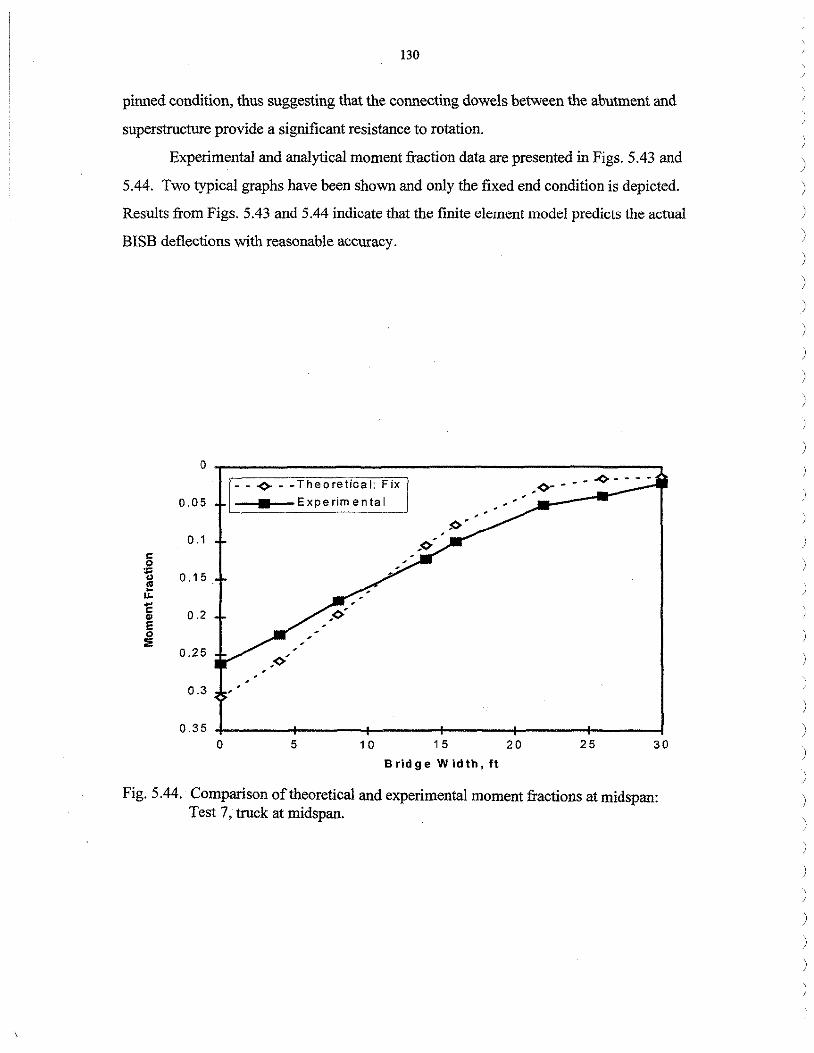
130
pinned condition, thus suggesting that the connecting dowels between the abutment and
superstructure provide a significant resistance to rotation.
Experimental and analytical moment fraction data are presented in Figs. 5.43 and
5.44. Two typical graphs have been shown and only the fixed end condition is depicted.
Results from Figs. 5.43 and 5.44 indicate that the finite element model predicts the actual
BISB deflections with reasonable accuracy.
0
~<> - -Theoretical: Fix <>- - - --<>----0.05 • Experim en ta I
0 .1
a ~ 0 .15 .. h u.. c 0.2 " E 0 :s
0.25 <>'
0.3
0.35 0 5 1 0 1 5 20 25 30
Bridge Width, ft
Fig. 5.44. Comparison of theoretical and experimental moment fractions at midspan: Test 7, truck at midspan.
)
)
)
)
)
131
6. SUMMARY AND CONCLUSIONS
In this phase of the investigation, Concept 2 - Beam-in-Slab Bridge - was
investigated. The study consisted of several tasks. In the experimental part of the
investigation, there were several types of static load tests: push-out tests, BISB
laboratory tests, composite beam tests, and a BISB field test. In the analytical part of the
study, a grillage method of analysis was used to develop analytical models of the four
beam BISB tested in the laboratory and the BISB tested in the field.
Although previous research has led to the development of a variety of design
equations for the shear strength of a shear hole connector, an evaluation of those
equations indicated that friction between the steel plate and the concrete was ignored, or
defined in terms of unknown quantities, such as the stress at an interface, which would
make use of the equation very difficult to use in design. A series of 36 push-out tests
were performed considering the following: hole size, amount of reinforcing steel through
the shear holes, amount of transverse slab reinforcement, concrete strength, and number
of shear holes. An equation was developed relating these five variables to the design
strength of a given connection.
The following conclusions are based on the results of the push-out tests:
• Separation of the concrete slabs and displacement of the steel plate were
negligible factors in the strength of the connector.
• Three distinct phases were noted in the loading of an ASC: nearly linear
stiffness phase, the point of maximum load, and a phase where the slip
increases with a corresponding decrease in the load.
• After the maximum load was attained, generally 80-90% of the maximum
load was retained at an average slip of7.6 mm (0.3 in.). After failure of the
concrete dowels, the friction between the concrete and steel plate and between
cracked concrete surfaces continued to provide shear resistance.
• The fabrication method used to create the shear holes had an insignificant
effect on the shear strength of the connector. Thus, torched holes can be used
with very minimal decrease in shear strength.
132
• Spacing of the holes had an insignificant effect on the shear strength of a
given ASC if a minimum spacing of 1. 7 times the shear hole diameter was
maintained.
• A significant strength increase, as well as an increase in the stiffuess, was
noted with an increase in the size of the shear hole.
• If designed correctly, the displacement between the concrete plate and the
steel plate (slip) will be minimal throughout service loading conditions and
failure will occur by shearing of the concrete dowels formed by concrete
penetrating the shear holes.
The BISB laboratory tests of the two-beam specimen (beams spaced 610 mm (2
ft) apart) included service load tests and an ultimate load test. The model bridge (L =
9,150 mm (30 ft), W = 915 mm (3 ft)) was simply supported and was subjected to two
point loading. Results from the two-beam specimen tests indicated the following
conclusions:
• In the early stages of loading, the specimen behaved like a composite beam.
At approximately 22.25 kN (5 kips), the specimen began to behave non
compositely, indicating that the bond between the steel and concrete had been
reduced. At a load of approximately 67 kN (15 kips), the specimen acted
essentially like a non-composite structure, with the concrete providing
minimal structural strength.
• Throughout service loading conditions, end slip was negligible. At loads
exceeding 40 kips, the end slip significantly increased with increasing load.
• The specimen ultimate load capacity was approximately 890 kN (200 kips)
total for the two point loading. This was the capacity of the loading system,
however, for all practical purposes the beam had failed as the steel had
yielded.
The BISB laboratory tests of the four-beam specimen (beams spaced 610 mm (2
ft) apart) also included both service load tests and an ultimate load test in which both
deflections and strains were measured. The ultimate load test was stopped when the steel
beams had yielded and the limit of the testing system had been reached. A grillage model
)
)
)
)
)
)
)
)
)
)
)
)
)
)
)
)
)
)
)
133
of the four-beam specimen was created and analytical results were compared to the
experimental results of the service level load tests.
The following conclusions can be made based on the four-beam specimen tests:
• The specimen behaved nonlinearly at loads above 1.33 MN (300 kips) and 73
mm (2.87 in.) of deflection at the centerline.
• The ultimate load capacity the specimen was 1.65 MN (370 kips) and the
deflection at this load was 103 mm (4.06 in.).
• The grillage analogy model provided predictions of the specimen deflections to
within 15% of the experimental results.
Four composite beam specimens were tested. Specimen 1 consisted of an inverted
T-section fabricated by cutting off a flange of a W21 x62 steel beam. The concrete slab
was cast on the top of the inverted T-section. Specimens 2 and 3 were constructed from
W21 x62 steel beams with their top flange imbedded into the concrete slab. The total
depth (from the top of slab to the bottom flange of the beam) of the specimens was the
same as Specimen 1. Specimen 4 was cast with a concrete slab cast directly on top of the
top flange of a W21 x62 steel beam using shear studs to attain composite action.
Specimens 1, 2, and 3 were also cast to attain composite action; however, they utilized
the new shear hole shear connector (ASC).
Each composite beam specimen was instrumented to measure strains and
deflections. Each specimen was loaded three times at service level conditions using a
two point loading arrangement, and then an ultimate load test was performed. The
ultimate load test concluded when the concrete failed in compression at the midspan of
the specimens.
The results from the composite beam tests indicated the following conclusions:
• The service level deflection of all three composite beam specimens was
accurately predicted to within 5% by assuming complete composite action.
• No change in the neutral axis location was observed during the service level
tests of all three specimens.
• The ASC shear hole shear connector is an effective shear transfer mechanism.

\
134
• The service load tests showed that the behavior of the composite beam
specimen utilizing the inverted T-section can be adequately modeled using
standard composite beam theory.
• The load/deflection behavior of all three types of composite beam specimens
was similar.
A field bridge with a span length of 15,240 mm (50 ft) was load tested using two
heavily loaded trucks. Both strain and deflections were recorded during the tests. An
analytical model of the bridge using the grillage method of analysis was developed and
results were compared with the experimental field bridge data.
The results from the testing indicated the following conclusions:
• The BISB system results in a very stiff structure both transversely and
longitudinally (the maximum bridge deflections was approximately 6 mm (1/4
in.) with a load of 445 kN (100 kips)).
• Load is distributed effectively transversely throughout the width of the
bridge.
• Theoretical analysis results from the grillage model of the bridge when
compared to the experimental load test data indicated that the bridge has a
significant amount of rotational fixity at each abutment.
)
)
)
)
)
)
)
)
)
)
)
)
)
)
)
)
)
)
)
)
)
)
)
)
)
' )
)

135
7. RECOMMENDED RESEARCH
On the basis of the work completed in this phase of the investigation, the
completion of the following tasks are recommended before this concept can be employed
in a demonstration project:
1. Additional laboratory tests are required. In these tests the following
variables should be investigated: post-tensioning of the steel beams to
create camber so that the system can be used on longer spans, T-sections
fabricated from W-shaped sections, and structural plates. In all the tests,
the ASC should be fabricated with torched holes.
2. A limited number of cyclic tests are needed. The majority of these should
be performed on push-out specimens; however, some should be performed
on full-scale composite beam specimens.
3. Using the results of the previous two tasks and the results from the Phase I
research, two and four beam composite specimens with fabricated T
sections, ASC, and various profiles of tension concrete should be
fabricated and tested. The tests should be service load tests as well as
ultimate load tests.
Assuming successful completion of these recommended three tasks, the next step
should be to use the modified BISB in a demonstration project.
137
8. ACKNOWLEDGEMENTS
The study presented in this report was conducted by the Bridge Engineering
Center under the auspices of the Engineering Research Institute of Iowa State University.
The research was sponsored by the Project Development Division of the Iowa
Department of Transportation and Iowa Highway Research Board under Research Project
382.
The authors wish to thank the various Iowa DOT and county engineers who
helped with this project and provided their input and support. In particular, we would
like to thank the project advisory committee:
• Dennis J. Edgar, Assistant County Engineer, Blackhawk County
• Robert L. Gumbert, County Engineer, Tama County
• Mark J. Nahra, County Engineer, Cedar County
• Gerald D. Petermeier, County Engineer, Benton County
• Wallace C. Mook, Director of Public Works, City of Bettendorf
• Jim Witt, County Engineer, Cerro Gordo County
Appreciation is also extended to Bruce L. Brakke and Vernon Marks of the Iowa
DOT for their assitance in obtaining the surplus steel beams used in this investigation.
Gerald D. Petermeier is also thanked for providing the field bridge for load testing and
the loaded trucks used in the testing.
Special thanks are accorded to the following Civil Engineering graduate and
undergraduate students and Construction Engineering undergraduate students for their
assistance in various aspects of the project: Andrea Heller, Trevor Brown, Matthew
Fagen, David Oxenford, Brett Conard, Matt Smith, Chris Kruse, Mary Walz, Penny
Moore, Dave Kepler, Ryan Paradis, Hillary Isebrands, Ted Willis, and Kevin Lex.
Brent Phares, graduate student in Civil Engineering is also thanked for his special efforts
in organizing this report. The authors also wish to thank Elaine Wipf for editing the
report and Denise Wood for typing the final manuscript.

9. REFERENCES
1. "Ninth Annual report to Congress-Highway Bridge Replacement and Rehabilitation Program", FHWA, Washington, D.C., 1989.
2. "Rural Bridges: An Assessment Based Upon the National Bridge Inventory". Transportation Report, United States Department of Agriculture, Office of Transportation, April 1989.
3. Wipf, T.J., Klaiber, F.W., Prabhakaran, A., "Evaluation of Bridge Replacement Alternatives for the County Bridge System". Iowa Department of Transportation Project HR-365, ISU-ERI-Ames 95403, Iowa State University, Ames, Iowa, 1994.
4. Leonhardt, E.F., Andra, W., Andra, H-P., Harre, W., "New Improved Shear Connector With High Fatigue Strength for Composite Structures (Neues, vorteilhaftes Verbundmittel fur Stahlverbund--Tragwerke rnit hoher Dauerfestigkeit)". Beton--Und Stahlbetonbau, Vol. 12, pp. 325-331, 1987.
5. Roberts, W.S., and Heywood, R.J., "An Innovation to Increase the Competitiveness of Short Span Steel Concrete Composite Bridges". Proceedings, Fourth International Conference on Short and Medium Span Bridges. Developments in Short and Medium Span Bridge Engineering '94, Halifax, Nova Scotia, Canada, pp. 1160-1171, 1994.
6. Antunes, P.J., Behavior of Perfobond Rib Connectors in Composite Beams. B.Sc. Thesis, University of Saskatchewan, Saskatoon, Canada, 1988.
7. Veldanda, M.R., and Hosain, M.U., "Behavior of Perfobond Rib Shear Connectors in Composite Beams: Push-out Tests". Canadian Journal of Civil Engineering, Vol. 19, pp. 1-10, 1992.
8. Oguejiofor, E.C., and Hosain, M.U., "Behavior of Perfobond Rib Shear Connectors in Composite Beams: Full Size Tests". Canadian Journal of Civil Engineering, Vol. 19, pp. 224-235, 1992.
9. Oguejiofor, E.C., and Hosain, M.U., "Perfobond Rib Connectors For Composite Beams". Proceedings. Engineering Foundation Conference on Composite Construction in Steel and Concrete II, Potosi, Mo. 1992, pp. 883-898.
10. Davies, C. Tests on half-scale steel-concrete composite beams with welded stud connectors. Structural Engineering, 47(1), pp. 29-40, 1969.
11. Slutter, R.G., and Driscoll, G.C. "Flexural Strength of Steel-Concrete Beams". American Society of Civil Engineers. Journal of the Structural Division, Vol. 91, No. ST2, April 1965. pp. 71-99.
12. Roberts, W.S., and Heywood, R.J., "Development and Testing of a New Shear Connector for Steel Concrete Composite Bridges". Proceedings, Fourth International Bridge Engineering Conference. 1994, pp. 137-145.
13. Standard Specification for Highway Bridges, American Association of State Highway and Transportation Officials (AASHTO), Sixteenth Edition, Washington, D.C., 1996.
14. Siess, C.P., Newmark, N.M., and Viest, l.M., "Small Scale Tests of Shear Connectors and Composite T-Beams". Studies of Slab and Beam Highway Bridges, Part III. University of Illinois Bulletin, Vol. 49, No. 45, Bulletin Series No. 396, February 1952.
15. Ollgard, Jorgan G., The Strength of Stud Shear Connectors in Nounal and Lightweight Concrete. M.S. Thesis, Lehigh University, Bethlehem, Pennsylvania, 1970.
16. Jaeger, L.G., and Bakht, B., Bridge Analysis by Microcomputer. McGraw-HiJI, New York, 1989.
17. ANSYS User's Manual for Revision 5.1. Swanson Analysis Systems, Inc., Houston, PA, 1992.
18. Yan, L.C.P., Design of Composite Steel-Concrete Structures, London: Surrey University Press, 1981.
)
)
)
)
)
)
)
)
)