g.1 introduction g-2

G.1 Introduction G-2

G.2 Vector Performance in More Depth G-2

G.3 Vector Memory Systems in More Depth G-9

G.4 Enhancing Vector Performance G-11

G.5 Effectiveness of Compiler Vectorization G-14

G.6 Putting It All Together: Performance of Vector Processors G-15

G.7 A Modern Vector Supercomputer: The Cray X1 G-21

G.8 Concluding Remarks G-25

G.9 Historical Perspective and References G-26

Exercises G-30

GVector Processors in More

Depth 2

Revised by Krste AsanovicMassachusetts Institute of Technology

I’m certainly not inventing vector processors. There are three kinds that I know of existing today. They are represented by the Illiac-IV, the (CDC) Star processor, and the TI (ASC) processor. Those three were all pioneering processors. . . . One of the problems of being a pioneer is you always make mistakes and I never, never want to be a pioneer. It’salways best to come second when you can look at the mistakes the pioneers made.

Seymour CrayPublic lecture at Lawrence Livermore Laboratories

on the introduction of the Cray-1 (1976)

G-2 ■ Appendix G Vector Processors in More Depth

Chapter 4 introduces vector architectures and places Multimedia SIMD exten-sions and GPUs in proper context to vector architectures.

In this appendix, we go into more detail on vector architectures, includingmore accurate performance models and descriptions of previous vector architec-tures. Figure G.1 shows the characteristics of some typical vector processors,including the size and count of the registers, the number and types of functionalunits, the number of load-store units, and the number of lanes.

The chime approximation is reasonably accurate for long vectors. Another sourceof overhead is far more significant than the issue limitation.

The most important source of overhead ignored by the chime model is vectorstart-up time. The start-up time comes from the pipelining latency of the vectoroperation and is principally determined by how deep the pipeline is for the func-tional unit used. The start-up time increases the effective time to execute a con-voy to more than one chime. Because of our assumption that convoys do notoverlap in time, the start-up time delays the execution of subsequent convoys. Ofcourse, the instructions in successive convoys either have structural conflicts forsome functional unit or are data dependent, so the assumption of no overlap isreasonable. The actual time to complete a convoy is determined by the sum of thevector length and the start-up time. If vector lengths were infinite, this start-upoverhead would be amortized, but finite vector lengths expose it, as the followingexample shows.

Example Assume that the start-up overhead for functional units is shown in Figure G.2.

Show the time that each convoy can begin and the total number of cycles needed.How does the time compare to the chime approximation for a vector of length 64?

Answer Figure G.3 provides the answer in convoys, assuming that the vector length is n.One tricky question is when we assume the vector sequence is done; this deter-mines whether the start-up time of the SV is visible or not. We assume that theinstructions following cannot fit in the same convoy, and we have alreadyassumed that convoys do not overlap. Thus, the total time is given by the timeuntil the last vector instruction in the last convoy completes. This is an approxi-mation, and the start-up time of the last vector instruction may be seen in somesequences and not in others. For simplicity, we always include it.

The time per result for a vector of length 64 is 4 + (42/64) = 4.65 clockcycles, while the chime approximation would be 4. The execution time with start-up overhead is 1.16 times higher.

G.1 Introduction

G.2 Vector Performance in More Depth

G.2 Vector Performance in More Depth ■ G-3

Processor (year)

Vectorclockrate

(MHz)Vector

registers

Elements perregister(64-bit

elements) Vector arithmetic units

Vectorload-store

units Lanes

Cray-1 (1976) 80 8 64 6: FP add, FP multiply, FP reciprocal, integer add, logical, shift

1 1

Cray X-MP (1983)

Cray Y-MP (1988)

118

1668 64

8: FP add, FP multiply, FP reciprocal, integer add, 2 logical, shift, population count/parity

2 loads1 store

1

Cray-2 (1985) 244 8 64 5: FP add, FP multiply, FP reciprocal/sqrt, integer add/shift/population count, logical

1 1

Fujitsu VP100/VP200 (1982)

133 8–256 32–1024 3: FP or integer add/logical, multiply, divide 2 1 (VP100)2 (VP200)

Hitachi S810/S820 (1983)

71 32 256 4: FP multiply-add, FP multiply/divide-add unit, 2 integer add/logical

3 loads1 store

1 (S810)2 (S820)

Convex C-1 (1985) 10 8 128 2: FP or integer multiply/divide, add/logical 1 1 (64 bit)2 (32 bit)

NEC SX/2 (1985) 167 8 + 32 256 4: FP multiply/divide, FP add, integer add/logical, shift

1 4

Cray C90 (1991)

Cray T90 (1995)

240

4608 128


2 loads1 store

2

NEC SX/5 (1998) 312 8 + 64 512 4: FP or integer add/shift, multiply, divide, logical

1 16

Fujitsu VPP5000 (1999)

300 8–256 128–4096 3: FP or integer multiply, add/logical, divide 1 load1 store

16

Cray SV1 (1998)

SV1ex (2001)

300

5008 64

(MSP)


1 load-store1 load

28 (MSP)

VMIPS (2001) 500 8 64 5: FP multiply, FP divide, FP add, integer add/shift, logical

1 load-store 1


1 8


1 4

Cray X1 (2002)

Cray XIE (2005)

800

113032

64256 (MSP)

3: FP or integer, add/logical, multiply/shift, divide/square root/logical

1 load1 store

28 (MSP)

Figure G.1 Characteristics of several vector-register architectures. If the machine is a multiprocessor, the entries correspond tothe characteristics of one processor. Several of the machines have different clock rates in the vector and scalar units; the clock ratesshown are for the vector units. The Fujitsu machines’ vector registers are configurable: The size and count of the 8K 64-bit entriesmay be varied inversely to one another (e.g., on the VP200, from eight registers each 1K elements long to 256 registers each 32 ele-ments long). The NEC machines have eight foreground vector registers connected to the arithmetic units plus 32 to 64 backgroundvector registers connected between the memory system and the foreground vector registers. Add pipelines perform add and sub-tract. The multiply/divide-add unit on the Hitachi S810/820 performs an FP multiply or divide followed by an add or subtract (whilethe multiply-add unit performs a multiply followed by an add or subtract). Note that most processors use the vector FP multiplyand divide units for vector integer multiply and divide, and several of the processors use the same units for FP scalar and FP vectoroperations. Each vector load-store unit represents the ability to do an independent, overlapped transfer to or from the vector regis-ters. The number of lanes is the number of parallel pipelines in each of the functional units as described in Section G.4. For example,the NEC SX/5 can complete 16 multiplies per cycle in the multiply functional unit. Several machines can split a 64-bit lane into two32-bit lanes to increase performance for applications that require only reduced precision. The Cray SV1 and Cray X1 can group fourCPUs with two lanes each to act in unison as a single larger CPU with eight lanes, which Cray calls a Multi-Streaming Processor(MSP).


For simplicity, we will use the chime approximation for running time, incor-porating start-up time effects only when we want performance that is moredetailed or to illustrate the benefits of some enhancement. For long vectors, a typ-ical situation, the overhead effect is not that large. Later in the appendix, we willexplore ways to reduce start-up overhead.

Start-up time for an instruction comes from the pipeline depth for the func-tional unit implementing that instruction. If the initiation rate is to be kept at 1clock cycle per result, then

For example, if an operation takes 10 clock cycles, it must be pipelined 10 deepto achieve an initiation rate of one per clock cycle. Pipeline depth, then, is deter-mined by the complexity of the operation and the clock cycle time of the proces-sor. The pipeline depths of functional units vary widely—2 to 20 stages arecommon—although the most heavily used units have pipeline depths of 4 to 8clock cycles.

For VMIPS, we will use the same pipeline depths as the Cray-1, althoughlatencies in more modern processors have tended to increase, especially forloads. All functional units are fully pipelined. From Chapter 4, pipeline depthsare 6 clock cycles for floating-point add and 7 clock cycles for floating-pointmultiply. On VMIPS, as on most vector processors, independent vector opera-tions using different functional units can issue in the same convoy.

In addition to the start-up overhead, we need to account for the overhead ofexecuting the strip-mined loop. This strip-mining overhead, which arises from

Unit Start-up overhead (cycles)

Load and store unit 12

Multiply unit 7

Add unit 6

Figure G.2 Start-up overhead.

Convoy Starting time First-result time Last-result time

1. LV 0 12 11 + n

2. MULVS.D LV 12 + n 12 + n + 12 23 + 2n

3. ADDV.D 24 + 2n 24 + 2n + 6 29 + 3n

4. SV 30 + 3n 30 + 3n + 12 41 + 4n

Figure G.3 Starting times and first- and last-result times for convoys 1 through 4.The vector length is n.

Pipeline depth Total functional unit timeClock cycle time

-------------------------------------------------------------=


the need to reinitiate the vector sequence and set the Vector Length Register(VLR) effectively adds to the vector start-up time, assuming that a convoy doesnot overlap with other instructions. If that overhead for a convoy is 10 cycles,then the effective overhead per 64 elements increases by 10 cycles, or 0.15 cyclesper element.

Two key factors contribute to the running time of a strip-mined loop consist-ing of a sequence of convoys:

1. The number of convoys in the loop, which determines the number of chimes.We use the notation Tchime for the execution time in chimes.

2. The overhead for each strip-mined sequence of convoys. This overhead con-sists of the cost of executing the scalar code for strip-mining each block,Tloop, plus the vector start-up cost for each convoy, Tstart.

There may also be a fixed overhead associated with setting up the vectorsequence the first time. In recent vector processors, this overhead has becomequite small, so we ignore it.

The components can be used to state the total running time for a vectorsequence operating on a vector of length n, which we will call Tn:

The values of Tstart, Tloop, and Tchime are compiler and processor dependent. Theregister allocation and scheduling of the instructions affect both what goes in aconvoy and the start-up overhead of each convoy.

For simplicity, we will use a constant value for Tloop on VMIPS. Based on avariety of measurements of Cray-1 vector execution, the value chosen is 15 forTloop. At first glance, you might think that this value is too small. The overhead ineach loop requires setting up the vector starting addresses and the strides, incre-menting counters, and executing a loop branch. In practice, these scalar instruc-tions can be totally or partially overlapped with the vector instructions,minimizing the time spent on these overhead functions. The value of Tloop ofcourse depends on the loop structure, but the dependence is slight compared withthe connection between the vector code and the values of Tchime and Tstart.

Operation Start-up penalty

Vector add 6

Vector multiply 7

Vector divide 20

Vector load 12

Figure G.4 Start-up penalties on VMIPS. These are the start-up penalties in clockcycles for VMIPS vector operations.

Tnn

MVL-------------- Tloop Tstart+

⎝ ⎠⎛ ⎞× n T× chime+=


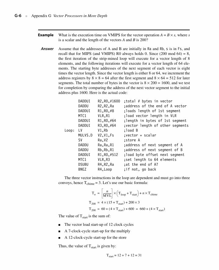
Example What is the execution time on VMIPS for the vector operation A = B × s, where sis a scalar and the length of the vectors A and B is 200?

Answer Assume that the addresses of A and B are initially in Ra and Rb, s is in Fs, andrecall that for MIPS (and VMIPS) R0 always holds 0. Since (200 mod 64) = 8,the first iteration of the strip-mined loop will execute for a vector length of 8elements, and the following iterations will execute for a vector length of 64 ele-ments. The starting byte addresses of the next segment of each vector is eighttimes the vector length. Since the vector length is either 8 or 64, we increment theaddress registers by 8 × 8 = 64 after the first segment and 8 × 64 = 512 for latersegments. The total number of bytes in the vector is 8 × 200 = 1600, and we testfor completion by comparing the address of the next vector segment to the initialaddress plus 1600. Here is the actual code:

DADDUI R2,R0,#1600 ;total # bytes in vectorDADDU R2,R2,Ra ;address of the end of A vectorDADDUI R1,R0,#8 ;loads length of 1st segmentMTC1 VLR,R1 ;load vector length in VLRDADDUI R1,R0,#64 ;length in bytes of 1st segmentDADDUI R3,R0,#64 ;vector length of other segments

Loop: LV V1,Rb ;load BMULVS.D V2,V1,Fs ;vector * scalarSV Ra,V2 ;store ADADDU Ra,Ra,R1 ;address of next segment of ADADDU Rb,Rb,R1 ;address of next segment of BDADDUI R1,R0,#512 ;load byte offset next segmentMTC1 VLR,R3 ;set length to 64 elementsDSUBU R4,R2,Ra ;at the end of A?BNEZ R4,Loop ;if not, go back

The three vector instructions in the loop are dependent and must go into threeconvoys, hence Tchime = 3. Let’s use our basic formula:

The value of Tstart is the sum of:

■ The vector load start-up of 12 clock cycles

■ A 7-clock-cycle start-up for the multiply

■ A 12-clock-cycle start-up for the store

Thus, the value of Tstart is given by:

Tstart = 12 + 7 + 12 = 31

Tnn


⎝ ⎠⎛ ⎞× n Tchime×+=

T200 4 15 Tstart+( ) 200 3×+×=

T200 60 4 Tstart×( ) 600+ + 660 4 Tstart×( )+= =


So, the overall value becomes:

T200 = 660 + 4 × 31= 784

The execution time per element with all start-up costs is then 784/200 = 3.9,compared with a chime approximation of three. In Section G.4, we will be moreambitious—allowing overlapping of separate convoys.

Figure G.5 shows the overhead and effective rates per element for the previ-ous example (A = B × s) with various vector lengths. A chime-counting modelwould lead to 3 clock cycles per element, while the two sources of overhead add0.9 clock cycles per element in the limit.

Pipelined Instruction Start-Up and Multiple Lanes

Adding multiple lanes increases peak performance but does not change start-uplatency, and so it becomes critical to reduce start-up overhead by allowing thestart of one vector instruction to be overlapped with the completion of precedingvector instructions. The simplest case to consider is when two vector instructionsaccess a different set of vector registers. For example, in the code sequence

ADDV.D V1,V2,V3ADDV.D V4,V5,V6

Figure G.5 The total execution time per element and the total overhead time perelement versus the vector length for the example on page F-6. For short vectors, thetotal start-up time is more than one-half of the total time, while for long vectors itreduces to about one-third of the total time. The sudden jumps occur when the vectorlength crosses a multiple of 64, forcing another iteration of the strip-mining code andexecution of a set of vector instructions. These operations increase Tn by Tloop + Tstart.

Total timeper element

Totaloverheadper element

10

Clockcycles

30 50 70 90 110 130 150 170 1900

1

2

3

4

5

6

7

8

Vector size

9


An implementation can allow the first element of the second vector instruction tofollow immediately the last element of the first vector instruction down the FPadder pipeline. To reduce the complexity of control logic, some vector machinesrequire some recovery time or dead time in between two vector instructions dis-patched to the same vector unit. Figure G.6 is a pipeline diagram that shows bothstart-up latency and dead time for a single vector pipeline.

The following example illustrates the impact of this dead time on achievablevector performance.

Example The Cray C90 has two lanes but requires 4 clock cycles of dead time between anytwo vector instructions to the same functional unit, even if they have no datadependences. For the maximum vector length of 128 elements, what is the reduc-tion in achievable peak performance caused by the dead time? What would be thereduction if the number of lanes were increased to 16?

Answer A maximum length vector of 128 elements is divided over the two lanes andoccupies a vector functional unit for 64 clock cycles. The dead time adds another4 cycles of occupancy, reducing the peak performance to 64/(64 + 4) = 94.1% ofthe value without dead time. If the number of lanes is increased to 16, maximumlength vector instructions will occupy a functional unit for only 128/16 = 8cycles, and the dead time will reduce peak performance to 8/(8 + 4) = 66.6% ofthe value without dead time. In this second case, the vector units can never bemore than 2/3 busy!

Figure G.6 Start-up latency and dead time for a single vector pipeline. Each elementhas a 5-cycle latency: 1 cycle to read the vector-register file, 3 cycles in execution, then1 cycle to write the vector-register file. Elements from the same vector instruction canfollow each other down the pipeline, but this machine inserts 4 cycles of dead timebetween two different vector instructions. The dead time can be eliminated with morecomplex control logic. (Reproduced with permission from Asanovic [1998].)

G.3 Vector Memory Systems in More Depth ■ G-9

Pipelining instruction start-up becomes more complicated when multipleinstructions can be reading and writing the same vector register and when someinstructions may stall unpredictably—for example, a vector load encounteringmemory bank conflicts. However, as both the number of lanes and pipeline laten-cies increase, it becomes increasingly important to allow fully pipelined instruc-tion start-up.

To maintain an initiation rate of one word fetched or stored per clock, the mem-ory system must be capable of producing or accepting this much data. As we sawin Chapter 4, this usually done by spreading accesses across multiple indepen-dent memory banks. Having significant numbers of banks is useful for dealingwith vector loads or stores that access rows or columns of data.

The desired access rate and the bank access time determined how many bankswere needed to access memory without stalls. This example shows how thesetimings work out in a vector processor.

Example Suppose we want to fetch a vector of 64 elements starting at byte address 136,and a memory access takes 6 clocks. How many memory banks must we have tosupport one fetch per clock cycle? With what addresses are the banks accessed?When will the various elements arrive at the CPU?

Answer Six clocks per access require at least 6 banks, but because we want the number ofbanks to be a power of 2, we choose to have 8 banks. Figure G.7 shows the tim-ing for the first few sets of accesses for an 8-bank system with a 6-clock-cycleaccess latency.

The timing of real memory banks is usually split into two different compo-nents, the access latency and the bank cycle time (or bank busy time). The accesslatency is the time from when the address arrives at the bank until the bankreturns a data value, while the busy time is the time the bank is occupied with onerequest. The access latency adds to the start-up cost of fetching a vector frommemory (the total memory latency also includes time to traverse the pipelinedinterconnection networks that transfer addresses and data between the CPU andmemory banks). The bank busy time governs the effective bandwidth of a mem-ory system because a processor cannot issue a second request to the same bankuntil the bank busy time has elapsed.

For simple unpipelined SRAM banks as used in the previous examples, theaccess latency and busy time are approximately the same. For a pipelined SRAMbank, however, the access latency is larger than the busy time because each ele-ment access only occupies one stage in the memory bank pipeline. For a DRAMbank, the access latency is usually shorter than the busy time because a DRAMneeds extra time to restore the read value after the destructive read operation. For

G.3 Vector Memory Systems in More Depth


memory systems that support multiple simultaneous vector accesses or allownonsequential accesses in vector loads or stores, the number of memory banksshould be larger than the minimum; otherwise, memory bank conflicts will exist.

Memory bank conflicts will not occur within a single vector memory instruc-tion if the stride and number of banks are relatively prime with respect to eachother and there are enough banks to avoid conflicts in the unit stride case. Whenthere are no bank conflicts, multiword and unit strides run at the same rates.Increasing the number of memory banks to a number greater than the minimumto prevent stalls with a stride of length 1 will decrease the stall frequency forsome other strides. For example, with 64 banks, a stride of 32 will stall on everyother access, rather than every access. If we originally had a stride of 8 and 16banks, every other access would stall; with 64 banks, a stride of 8 will stall onevery eighth access. If we have multiple memory pipelines and/or multiple pro-cessors sharing the same memory system, we will also need more banks to pre-vent conflicts. Even machines with a single memory pipeline can experiencememory bank conflicts on unit stride accesses between the last few elements of

Bank

Cycle no. 0 1 2 3 4 5 6 7

0 136

1 Busy 144

2 Busy Busy 152

3 Busy Busy Busy 160

4 Busy Busy Busy Busy 168

5 Busy Busy Busy Busy Busy 176


7 192 Busy Busy Busy Busy Busy

8 Busy 200 Busy Busy Busy Busy

9 Busy Busy 208 Busy Busy Busy

10 Busy Busy Busy 216 Busy Busy

11 Busy Busy Busy Busy 224 Busy




15 256 Busy Busy Busy Busy Busy

16 Busy 264 Busy Busy Busy Busy

Figure G.7 Memory addresses (in bytes) by bank number and time slot at whichaccess begins. Each memory bank latches the element address at the start of an accessand is then busy for 6 clock cycles before returning a value to the CPU. Note that theCPU cannot keep all 8 banks busy all the time because it is limited to supplying onenew address and receiving one data item each cycle.

G.4 Enhancing Vector Performance ■ G-11

one instruction and the first few elements of the next instruction, and increasingthe number of banks will reduce the probability of these inter-instruction con-flicts. In 2011, most vector supercomputers spread the accesses from each CPUacross hundreds of memory banks. Because bank conflicts can still occur in non-unit stride cases, programmers favor unit stride accesses whenever possible.

A modern supercomputer may have dozens of CPUs, each with multiplememory pipelines connected to thousands of memory banks. It would be imprac-tical to provide a dedicated path between each memory pipeline and each mem-ory bank, so, typically, a multistage switching network is used to connectmemory pipelines to memory banks. Congestion can arise in this switching net-work as different vector accesses contend for the same circuit paths, causingadditional stalls in the memory system.

In this section, we present techniques for improving the performance of a vectorprocessor in more depth than we did in Chapter 4.

Chaining in More Depth

Early implementations of chaining worked like forwarding, but this restricted thetiming of the source and destination instructions in the chain. Recent implemen-tations use flexible chaining, which allows a vector instruction to chain to essen-tially any other active vector instruction, assuming that no structural hazard isgenerated. Flexible chaining requires simultaneous access to the same vector reg-ister by different vector instructions, which can be implemented either by addingmore read and write ports or by organizing the vector-register file storage intointerleaved banks in a similar way to the memory system. We assume this type ofchaining throughout the rest of this appendix.

Even though a pair of operations depends on one another, chaining allows theoperations to proceed in parallel on separate elements of the vector. This permitsthe operations to be scheduled in the same convoy and reduces the number ofchimes required. For the previous sequence, a sustained rate (ignoring start-up)of two floating-point operations per clock cycle, or one chime, can be achieved,even though the operations are dependent! The total running time for the abovesequence becomes:

Vector length + Start-up timeADDV + Start-up timeMULV

Figure G.8 shows the timing of a chained and an unchained version of the abovepair of vector instructions with a vector length of 64. This convoy requires onechime; however, because it uses chaining, the start-up overhead will be seen inthe actual timing of the convoy. In Figure G.8, the total time for chained opera-tion is 77 clock cycles, or 1.2 cycles per result. With 128 floating-point opera-tions done in that time, 1.7 FLOPS per clock cycle are obtained. For theunchained version, there are 141 clock cycles, or 0.9 FLOPS per clock cycle.

G.4 Enhancing Vector Performance


Although chaining allows us to reduce the chime component of the executiontime by putting two dependent instructions in the same convoy, it does noteliminate the start-up overhead. If we want an accurate running time estimate, wemust count the start-up time both within and across convoys. With chaining, thenumber of chimes for a sequence is determined by the number of different vectorfunctional units available in the processor and the number required by the appli-cation. In particular, no convoy can contain a structural hazard. This means, forexample, that a sequence containing two vector memory instructions must take atleast two convoys, and hence two chimes, on a processor like VMIPS with onlyone vector load-store unit.

Chaining is so important that every modern vector processor supports flexiblechaining.

Sparse Matrices in More Depth

Chapter 4 shows techniques to allow programs with sparse matrices to execute invector mode. Let’s start with a quick review. In a sparse matrix, the elements of avector are usually stored in some compacted form and then accessed indirectly.Assuming a simplified sparse structure, we might see code that looks like this:

do 100 i = 1,n100 A(K(i)) = A(K(i)) + C(M(i))

This code implements a sparse vector sum on the arrays A and C, using index vec-tors K and M to designate the nonzero elements of A and C. (A and C must have thesame number of nonzero elements—n of them.) Another common representationfor sparse matrices uses a bit vector to show which elements exist and a densevector for the nonzero elements. Often both representations exist in the same pro-gram. Sparse matrices are found in many codes, and there are many ways toimplement them, depending on the data structure used in the program.

A simple vectorizing compiler could not automatically vectorize the sourcecode above because the compiler would not know that the elements of K are dis-tinct values and thus that no dependences exist. Instead, a programmer directivewould tell the compiler that it could run the loop in vector mode.

More sophisticated vectorizing compilers can vectorize the loop automati-cally without programmer annotations by inserting run time checks for data

Figure G.8 Timings for a sequence of dependent vector operations ADDV and MULV,both unchained and chained. The 6- and 7-clock-cycle delays are the latency of theadder and multiplier.

Unchained

Chained

Total = 77

Total = 1417 64

7 64

MULV

64

ADDV

64

MULV ADDV

6

6

G.4 Enhancing Vector Performance ■ G-13

dependences. These run time checks are implemented with a vectorized softwareversion of the advanced load address table (ALAT) hardware described in Appen-dix H for the Itanium processor. The associative ALAT hardware is replaced witha software hash table that detects if two element accesses within the same strip-mine iteration are to the same address. If no dependences are detected, the strip-mine iteration can complete using the maximum vector length. If a dependence isdetected, the vector length is reset to a smaller value that avoids all dependencyviolations, leaving the remaining elements to be handled on the next iteration ofthe strip-mined loop. Although this scheme adds considerable software overheadto the loop, the overhead is mostly vectorized for the common case where thereare no dependences; as a result, the loop still runs considerably faster than scalarcode (although much slower than if a programmer directive was provided).

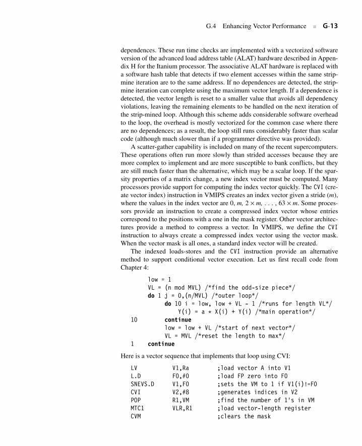
A scatter-gather capability is included on many of the recent supercomputers.These operations often run more slowly than strided accesses because they aremore complex to implement and are more susceptible to bank conflicts, but theyare still much faster than the alternative, which may be a scalar loop. If the spar-sity properties of a matrix change, a new index vector must be computed. Manyprocessors provide support for computing the index vector quickly. The CVI (cre-ate vector index) instruction in VMIPS creates an index vector given a stride (m),where the values in the index vector are 0, m, 2 × m, . . . , 63 × m. Some proces-sors provide an instruction to create a compressed index vector whose entriescorrespond to the positions with a one in the mask register. Other vector architec-tures provide a method to compress a vector. In VMIPS, we define the CVIinstruction to always create a compressed index vector using the vector mask.When the vector mask is all ones, a standard index vector will be created.

The indexed loads-stores and the CVI instruction provide an alternativemethod to support conditional vector execution. Let us first recall code fromChapter 4:

low = 1VL = (n mod MVL) /*find the odd-size piece*/do 1 j = 0,(n/MVL) /*outer loop*/

do 10 i = low, low + VL - 1 /*runs for length VL*/Y(i) = a * X(i) + Y(i) /*main operation*/

10 continuelow = low + VL /*start of next vector*/VL = MVL /*reset the length to max*/

1 continue

Here is a vector sequence that implements that loop using CVI:

LV V1,Ra ;load vector A into V1L.D F0,#0 ;load FP zero into F0SNEVS.D V1,F0 ;sets the VM to 1 if V1(i)!=F0 CVI V2,#8 ;generates indices in V2POP R1,VM ;find the number of 1’s in VMMTC1 VLR,R1 ;load vector-length registerCVM ;clears the mask


LVI V3,(Ra+V2) ;load the nonzero A elementsLVI V4,(Rb+V2) ;load corresponding B elementsSUBV.D V3,V3,V4 ;do the subtractSVI (Ra+V2),V3 ;store A back

Whether the implementation using scatter-gather is better than the condition-ally executed version depends on the frequency with which the condition holdsand the cost of the operations. Ignoring chaining, the running time of the originalversion is 5n + c1. The running time of the second version, using indexed loadsand stores with a running time of one element per clock, is 4n + 4fn + c2, where fis the fraction of elements for which the condition is true (i.e., A(i) ¦ 0). If weassume that the values of c1 and c2 are comparable, or that they are much smallerthan n, we can find when this second technique is better.

We want Time1 > Time2, so

That is, the second method is faster if less than one-quarter of the elements arenonzero. In many cases, the frequency of execution is much lower. If the indexvector can be reused, or if the number of vector statements within the if statementgrows, the advantage of the scatter-gather approach will increase sharply.

Two factors affect the success with which a program can be run in vector mode.The first factor is the structure of the program itself: Do the loops have true datadependences, or can they be restructured so as not to have such dependences?This factor is influenced by the algorithms chosen and, to some extent, by howthey are coded. The second factor is the capability of the compiler. While nocompiler can vectorize a loop where no parallelism among the loop iterationsexists, there is tremendous variation in the ability of compilers to determinewhether a loop can be vectorized. The techniques used to vectorize programs arethe same as those discussed in Chapter 3 for uncovering ILP; here, we simplyreview how well these techniques work.

There is tremendous variation in how well different compilers do in vectoriz-ing programs. As a summary of the state of vectorizing compilers, consider thedata in Figure G.9, which shows the extent of vectorization for different proces-sors using a test suite of 100 handwritten FORTRAN kernels. The kernels weredesigned to test vectorization capability and can all be vectorized by hand; wewill see several examples of these loops in the exercises.

Time1 5 n( )=

Time2 4n 4fn+=

5n 4n 4fn+>14--- f>

G.5 Effectiveness of Compiler Vectorization

G.6 Putting It All Together: Performance of Vector Processors ■ G-15

In this section, we look at performance measures for vector processors and whatthey tell us about the processors. To determine the performance of a processor ona vector problem we must look at the start-up cost and the sustained rate. Thesimplest and best way to report the performance of a vector processor on a loop isto give the execution time of the vector loop. For vector loops, people often givethe MFLOPS (millions of floating-point operations per second) rating rather thanexecution time. We use the notation Rn for the MFLOPS rating on a vector oflength n. Using the measurements Tn (time) or Rn (rate) is equivalent if the num-ber of FLOPS is agreed upon. In any event, either measurement should includethe overhead.

In this section, we examine the performance of VMIPS on a DAXPY loop(see Chapter 4) by looking at performance from different viewpoints. We willcontinue to compute the execution time of a vector loop using the equation devel-oped in Section G.2. At the same time, we will look at different ways to measureperformance using the computed time. The constant values for Tloop used in thissection introduce some small amount of error, which will be ignored.

Measures of Vector Performance

Because vector length is so important in establishing the performance of a pro-cessor, length-related measures are often applied in addition to time and

Processor CompilerCompletelyvectorized

Partially vectorized

Notvectorized

CDC CYBER 205 VAST-2 V2.21 62 5 33

Convex C-series FC5.0 69 5 26

Cray X-MP CFT77 V3.0 69 3 28

Cray X-MP CFT V1.15 50 1 49

Cray-2 CFT2 V3.1a 27 1 72

ETA-10 FTN 77 V1.0 62 7 31

Hitachi S810/820 FORT77/HAP V20-2B 67 4 29

IBM 3090/VF VS FORTRAN V2.4 52 4 44

NEC SX/2 FORTRAN77 / SX V.040 66 5 29

Figure G.9 Result of applying vectorizing compilers to the 100 FORTRAN test ker-nels. For each processor we indicate how many loops were completely vectorized, par-tially vectorized, and unvectorized. These loops were collected by Callahan, Dongarra,and Levine [1988]. Two different compilers for the Cray X-MP show the large depen-dence on compiler technology.

G.6 Putting It All Together: Performance of Vector Processors


MFLOPS. These length-related measures tend to vary dramatically across differ-ent processors and are interesting to compare. (Remember, though, that time isalways the measure of interest when comparing the relative speed of two proces-sors.) Three of the most important length-related measures are

■ R∞—The MFLOPS rate on an infinite-length vector. Although this measuremay be of interest when estimating peak performance, real problems havelimited vector lengths, and the overhead penalties encountered in real prob-lems will be larger.

■ N1/2—The vector length needed to reach one-half of R∞. This is a good mea-sure of the impact of overhead.

■ Nv—The vector length needed to make vector mode faster than scalar mode.This measures both overhead and the speed of scalars relative to vectors.

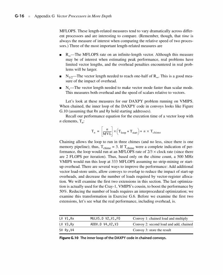
Let’s look at these measures for our DAXPY problem running on VMIPS.When chained, the inner loop of the DAXPY code in convoys looks like FigureG.10 (assuming that Rx and Ry hold starting addresses).

Recall our performance equation for the execution time of a vector loop withn elements, Tn:

Chaining allows the loop to run in three chimes (and no less, since there is onememory pipeline); thus, Tchime = 3. If Tchime were a complete indication of per-formance, the loop would run at an MFLOPS rate of 2/3 × clock rate (since thereare 2 FLOPS per iteration). Thus, based only on the chime count, a 500 MHzVMIPS would run this loop at 333 MFLOPS assuming no strip-mining or start-up overhead. There are several ways to improve the performance: Add additionalvector load-store units, allow convoys to overlap to reduce the impact of start-upoverheads, and decrease the number of loads required by vector-register alloca-tion. We will examine the first two extensions in this section. The last optimiza-tion is actually used for the Cray-1, VMIPS’s cousin, to boost the performance by50%. Reducing the number of loads requires an interprocedural optimization; weexamine this transformation in Exercise G.6. Before we examine the first twoextensions, let’s see what the real performance, including overhead, is.

LV V1,Rx MULVS.D V2,V1,F0 Convoy 1: chained load and multiply

LV V3,Ry ADDV.D V4,V2,V3 Convoy 2: second load and add, chained

SV Ry,V4 Convoy 3: store the result

Figure G.10 The inner loop of the DAXPY code in chained convoys.

Tnn


⎝ ⎠⎛ ⎞× n Tchime×+=


The Peak Performance of VMIPS on DAXPY

First, we should determine what the peak performance, R∞, really is, since weknow it must differ from the ideal 333 MFLOPS rate. For now, we continue touse the simplifying assumption that a convoy cannot start until all the instructionsin an earlier convoy have completed; later we will remove this restriction. Usingthis simplification, the start-up overhead for the vector sequence is simply thesum of the start-up times of the instructions:

Using MVL = 64, Tloop = 15, Tstart = 49, and Tchime = 3 in the performanceequation, and assuming that n is not an exact multiple of 64, the time for an n-element operation is

The sustained rate is actually over 4 clock cycles per iteration, rather than thetheoretical rate of 3 chimes, which ignores overhead. The major part of the differ-ence is the cost of the start-up overhead for each block of 64 elements (49 cyclesversus 15 for the loop overhead).

We can now compute R∞ for a 500 MHz clock as:

The numerator is independent of n, hence

The performance without the start-up overhead, which is the peak performancegiven the vector functional unit structure, is now 1.33 times higher. In actuality, thegap between peak and sustained performance for this benchmark is even larger!

Sustained Performance of VMIPS on the Linpack Benchmark

The Linpack benchmark is a Gaussian elimination on a 100 × 100 matrix. Thus,the vector element lengths range from 99 down to 1. A vector of length k is usedk times. Thus, the average vector length is given by:

Tstart 12 7 12 6 12+ + + + 49= =

Tnn64------ 15 49+( ) 3n+×=

n 64+( )≤ 3n+

4n 64+=

R∞Operations per iteration Clock rate×

Clock cycles per iteration----------------------------------------------------------------------------------------⎝ ⎠⎛ ⎞

n ∞→lim=


Clock cycles per iteration( )n ∞→lim

----------------------------------------------------------------------------------------=


Tn

n------⎝ ⎠⎛ ⎞

n ∞→lim

4n 64+n

------------------⎝ ⎠⎛ ⎞

n ∞→lim 4= = =

R∞2 500 MHz×

4-------------------------------- 250 MFLOPS= =


Now we can obtain an accurate estimate of the performance of DAXPY using avector length of 66:

The peak number, ignoring start-up overhead, is 1.64 times higher than thisestimate of sustained performance on the real vector lengths. In actual practice,the Linpack benchmark contains a nontrivial fraction of code that cannot be vec-torized. Although this code accounts for less than 20% of the time before vector-ization, it runs at less than one-tenth of the performance when counted asFLOPS. Thus, Amdahl’s law tells us that the overall performance will be signifi-cantly lower than the performance estimated from analyzing the inner loop.

Since vector length has a significant impact on performance, the N1/2 and Nvmeasures are often used in comparing vector machines.

Example What is N1/2 for just the inner loop of DAXPY for VMIPS with a 500 MHz clock?

Answer Using R∞ as the peak rate, we want to know the vector length that will achieveabout 125 MFLOPS. We start with the formula for MFLOPS assuming that themeasurement is made for N1/2 elements:

Simplifying this and then assuming N1/2 < 64, so that TN1/2 < 64 = 64 + 3 × n,yields:

So N1/2 = 13; that is, a vector of length 13 gives approximately one-half the peakperformance for the DAXPY loop on VMIPS.

i2

i 1=

99

∑

i

i 1=

99

∑

-------------- 66.3=

T66 2 15 49+( ) 66 3×+× 128 198+ 326= = =

R662 66 500××

326------------------------------ MFLOPS 202 MFLOPS= =

MFLOPSFLOPS executed in N1 2⁄ iterations

Clock cycles to execute N1 2⁄ iterations--------------------------------------------------------------------------------------------------

Clock cyclesSecond

------------------------------ 106–××=

1252 N1 2⁄×

TN1 2⁄

--------------------- 500×=

TN1 2⁄8 N1 2⁄×=

64 3 N1 2⁄×+ 8 N1 2⁄×=

5 N1 2⁄× 64=

N1 2⁄ 12.8=


Example What is the vector length, Nv, such that the vector operation runs faster than thescalar?

Answer Again, we know that Nv < 64. The time to do one iteration in scalar mode can beestimated as 10 + 12 + 12 + 7 + 6 +12 = 59 clocks, where 10 is the estimate of theloop overhead, known to be somewhat less than the strip-mining loop overhead. Inthe last problem, we showed that this vector loop runs in vector mode in timeTn ≤ 64 = 64 + 3 × n clock cycles. Therefore,

For the DAXPY loop, vector mode is faster than scalar as long as the vector hasat least two elements. This number is surprisingly small.

DAXPY Performance on an Enhanced VMIPS

DAXPY, like many vector problems, is memory limited. Consequently, per-formance could be improved by adding more memory access pipelines. This isthe major architectural difference between the Cray X-MP (and later processors)and the Cray-1. The Cray X-MP has three memory pipelines, compared with theCray-1’s single memory pipeline, and the X-MP has more flexible chaining. Howdoes this affect performance?

Example What would be the value of T66 for DAXPY on VMIPS if we added two morememory pipelines?

Answer With three memory pipelines, all the instructions fit in one convoy and take onechime. The start-up overheads are the same, so

With three memory pipelines, we have reduced the clock cycle count for sus-tained performance from 326 to 194, a factor of 1.7. Note the effect of Amdahl’slaw: We improved the theoretical peak rate as measured by the number of chimesby a factor of 3, but only achieved an overall improvement of a factor of 1.7 insustained performance.

64 3Nv+ 59Nv=

Nv6456------=

Nv 2=

T666664------ Tloop Tstart+

⎝ ⎠⎛ ⎞ 66 Tchime×+×=

T66 2 15 49+( ) 66 1×+× 194= =


Another improvement could come from allowing different convoys to overlapand also allowing the scalar loop overhead to overlap with the vector instructions.This requires that one vector operation be allowed to begin using a functionalunit before another operation has completed, which complicates the instructionissue logic. Allowing this overlap eliminates the separate start-up overhead forevery convoy except the first and hides the loop overhead as well.

To achieve the maximum hiding of strip-mining overhead, we need to be ableto overlap strip-mined instances of the loop, allowing two instances of a convoyas well as possibly two instances of the scalar code to be in execution simultane-ously. This requires the same techniques we looked at in Chapter 3 to avoid WARhazards, although because no overlapped read and write of a single vector ele-ment is possible, copying can be avoided. This technique, called tailgating, wasused in the Cray-2. Alternatively, we could unroll the outer loop to create severalinstances of the vector sequence using different register sets (assuming sufficientregisters), just as we did in Chapter 3. By allowing maximum overlap of the con-voys and the scalar loop overhead, the start-up and loop overheads will only beseen once per vector sequence, independent of the number of convoys and theinstructions in each convoy. In this way, a processor with vector registers canhave both low start-up overhead for short vectors and high peak performance forvery long vectors.

Example What would be the values of R∞ and T66 for DAXPY on VMIPS if we added two

more memory pipelines and allowed the strip-mining and start-up overheads tobe fully overlapped?

Answer

Since the overhead is only seen once, Tn = n + 49 + 15 = n + 64. Thus,

Adding the extra memory pipelines and more flexible issue logic yields animprovement in peak performance of a factor of 4. However, T66 = 130, so forshorter vectors the sustained performance improvement is about 326/130 = 2.5times.


Clock cycles per iteration----------------------------------------------------------------------------------------⎝ ⎠⎛ ⎞

n ∞→lim=


Tn

n------⎝ ⎠⎛ ⎞

n ∞→lim=

Tn

n------⎝ ⎠⎛ ⎞

n ∞→lim

n 64+n

---------------⎝ ⎠⎛ ⎞

n ∞→lim 1= =

R∞2 500 MHz×

1-------------------------------- 1000 MFLOPS= =

G.7 A Modern Vector Supercomputer: The Cray X1 ■ G-21

In summary, we have examined several measures of vector performance.Theoretical peak performance can be calculated based purely on the value ofTchime as:

By including the loop overhead, we can calculate values for peak performancefor an infinite-length vector (R∞) and also for sustained performance, Rn for avector of length n, which is computed as:

Using these measures we also can find N1/2 and Nv, which give us another way oflooking at the start-up overhead for vectors and the ratio of vector to scalar speed.A wide variety of measures of performance of vector processors is useful inunderstanding the range of performance that applications may see on a vectorprocessor.

The Cray X1 was introduced in 2002, and, together with the NEC SX/8, repre-sents the state of the art in modern vector supercomputers. The X1 system archi-tecture supports thousands of powerful vector processors sharing a single globalmemory.

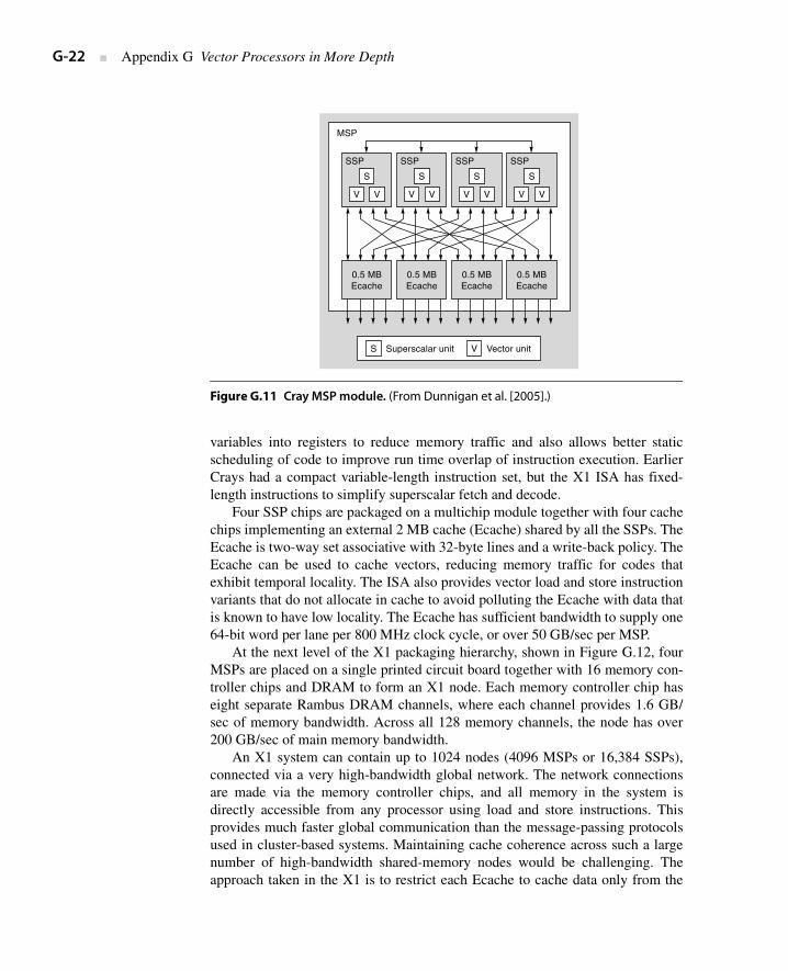
The Cray X1 has an unusual processor architecture, shown in Figure G.11. Alarge Multi-Streaming Processor (MSP) is formed by ganging together four Sin-gle-Streaming Processors (SSPs). Each SSP is a complete single-chip vectormicroprocessor, containing a scalar unit, scalar caches, and a two-lane vectorunit. The SSP scalar unit is a dual-issue out-of-order superscalar processor with a16 KB instruction cache and a 16 KB scalar write-through data cache, both two-way set associative with 32-byte cache lines. The SSP vector unit contains a vec-tor register file, three vector arithmetic units, and one vector load-store unit. It ismuch easier to pipeline deeply a vector functional unit than a superscalar issuemechanism, so the X1 vector unit runs at twice the clock rate (800 MHz) of thescalar unit (400 MHz). Each lane can perform a 64-bit floating-point add and a64-bit floating-point multiply each cycle, leading to a peak performance of 12.8GFLOPS per MSP.

All previous Cray machines could trace their instruction set architecture(ISA) lineage back to the original Cray-1 design from 1976, with 8 primary regis-ters each for addresses, scalar data, and vector data. For the X1, the ISA wasredesigned from scratch to incorporate lessons learned over the last 30 years ofcompiler and microarchitecture research. The X1 ISA includes 64 64-bit scalaraddress registers and 64 64-bit scalar data registers, with 32 vector data registers(64 bits per element) and 8 vector mask registers (1 bit per element). The largeincrease in the number of registers allows the compiler to map more program

Number of FLOPS per iteration Clock rate×Tchime

-----------------------------------------------------------------------------------------------------------

RnNumber of FLOPS per iteration n× Clock rate×

Tn--------------------------------------------------------------------------------------------------------------------=

G.7 A Modern Vector Supercomputer: The Cray X1


variables into registers to reduce memory traffic and also allows better staticscheduling of code to improve run time overlap of instruction execution. EarlierCrays had a compact variable-length instruction set, but the X1 ISA has fixed-length instructions to simplify superscalar fetch and decode.

Four SSP chips are packaged on a multichip module together with four cachechips implementing an external 2 MB cache (Ecache) shared by all the SSPs. TheEcache is two-way set associative with 32-byte lines and a write-back policy. TheEcache can be used to cache vectors, reducing memory traffic for codes thatexhibit temporal locality. The ISA also provides vector load and store instructionvariants that do not allocate in cache to avoid polluting the Ecache with data thatis known to have low locality. The Ecache has sufficient bandwidth to supply one64-bit word per lane per 800 MHz clock cycle, or over 50 GB/sec per MSP.

At the next level of the X1 packaging hierarchy, shown in Figure G.12, fourMSPs are placed on a single printed circuit board together with 16 memory con-troller chips and DRAM to form an X1 node. Each memory controller chip haseight separate Rambus DRAM channels, where each channel provides 1.6 GB/sec of memory bandwidth. Across all 128 memory channels, the node has over200 GB/sec of main memory bandwidth.

An X1 system can contain up to 1024 nodes (4096 MSPs or 16,384 SSPs),connected via a very high-bandwidth global network. The network connectionsare made via the memory controller chips, and all memory in the system isdirectly accessible from any processor using load and store instructions. Thisprovides much faster global communication than the message-passing protocolsused in cluster-based systems. Maintaining cache coherence across such a largenumber of high-bandwidth shared-memory nodes would be challenging. Theapproach taken in the X1 is to restrict each Ecache to cache data only from the

Figure G.11 Cray MSP module. (From Dunnigan et al. [2005].)

MSP

SSP

S

S Superscalar unit V Vector unit

V V

SSP

S

V V

SSP

S

V V

SSP

S

V V

0.5 MBEcache

0.5 MBEcache

0.5 MBEcache

0.5 MBEcache

G.7 A Modern Vector Supercomputer: The Cray X1 ■ G-23

local node DRAM. The memory controllers implement a directory scheme tomaintain coherency between the four Ecaches on a node. Accesses from remotenodes will obtain the most recent version of a location, and remote stores willinvalidate local Ecaches before updating memory, but the remote node cannotcache these local locations.

Vector loads and stores are particularly useful in the presence of long-latencycache misses and global communications, as relatively simple vector hardwarecan generate and track a large number of in-flight memory requests. Contempo-rary superscalar microprocessors support only 8 to 16 outstanding cache misses,whereas each MSP processor can have up to 2048 outstanding memory requests(512 per SSP). To compensate, superscalar microprocessors have been moving tolarger cache line sizes (128 bytes and above) to bring in more data with eachcache miss, but this leads to significant wasted bandwidth on non-unit strideaccesses over large datasets. The X1 design uses short 32-byte lines throughoutto reduce bandwidth waste and instead relies on supporting many independentcache misses to sustain memory bandwidth. This latency tolerance together withthe huge memory bandwidth for non-unit strides explains why vector machinescan provide large speedups over superscalar microprocessors for certain codes.

Multi-Streaming Processors

The Multi-Streaming concept was first introduced by Cray in the SV1, but hasbeen considerably enhanced in the X1. The four SSPs within an MSP shareEcache, and there is hardware support for barrier synchronization across the fourSSPs within an MSP. Each X1 SSP has a two-lane vector unit with 32 vector reg-isters each holding 64 elements. The compiler has several choices as to how touse the SSPs within an MSP.

Figure G.12 Cray X1 node. (From Tanqueray [2002].)

M

mem

M

mem

M

mem

M

mem

M

mem

M

mem

M

mem

M

mem

M

mem

M

mem

M

mem

M

mem

M

mem

M

mem

M

mem

M

mem

51 GFLOPS, 200 GB/secIOIO IO

P P P P

S S S S

P P P P

S S S S

P P P P

S S S S

P P P P

S S S S


The simplest use is to gang together four two-lane SSPs to emulate a singleeight-lane vector processor. The X1 provides efficient barrier synchronizationprimitives between SSPs on a node, and the compiler is responsible for generat-ing the MSP code. For example, for a vectorizable inner loop over 1000 ele-ments, the compiler will allocate iterations 0–249 to SSP0, iterations 250–499 toSSP1, iterations 500–749 to SSP2, and iterations 750–999 to SSP3. Each SSPcan process its loop iterations independently but must synchronize back with theother SSPs before moving to the next loop nest.

If inner loops do not have many iterations, the eight-lane MSP will have lowefficiency, as each SSP will have only a few elements to process and executiontime will be dominated by start-up time and synchronization overheads. Anotherway to use an MSP is for the compiler to parallelize across an outer loop, givingeach SSP a different inner loop to process. For example, the following nestedloops scale the upper triangle of a matrix by a constant:

/* Scale upper triangle by constant K. */for (row = 0; row < MAX_ROWS; row++)

for (col = row; col < MAX_COLS; col++)A[row][col] = A[row][col] * K;

Consider the case where MAX_ROWS and MAX_COLS are both 100 elements. Thevector length of the inner loop steps down from 100 to 1 over the iterations of theouter loop. Even for the first inner loop, the loop length would be much less thanthe maximum vector length (256) of an eight-lane MSP, and the code wouldtherefore be inefficient. Alternatively, the compiler can assign entire inner loopsto a single SSP. For example, SSP0 might process rows 0, 4, 8, and so on, whileSSP1 processes rows 1, 5, 9, and so on. Each SSP now sees a longer vector. Ineffect, this approach parallelizes the scalar overhead and makes use of the indi-vidual scalar units within each SSP.

Most application code uses MSPs, but it is also possible to compile code touse all the SSPs as individual processors where there is limited vector parallelismbut significant thread-level parallelism.

Cray X1E

In 2004, Cray announced an upgrade to the original Cray X1 design. The X1Euses newer fabrication technology that allows two SSPs to be placed on a singlechip, making the X1E the first multicore vector microprocessor. Each physicalnode now contains eight MSPs, but these are organized as two logical nodes offour MSPs each to retain the same programming model as the X1. In addition,the clock rates were raised from 400 MHz scalar and 800 MHz vector to565 MHz scalar and 1130 MHz vector, giving an improved peak performance of18 GFLOPS.

G.8 Concluding Remarks ■ G-25

During the 1980s and 1990s, rapid performance increases in pipelined scalarprocessors led to a dramatic closing of the gap between traditional vectorsupercomputers and fast, pipelined, superscalar VLSI microprocessors. In2011, it is possible to buy a laptop computer for under $1000 that has a higherCPU clock rate than any available vector supercomputer, even those costingtens of millions of dollars. Although the vector supercomputers have lowerclock rates, they support greater parallelism using multiple lanes (up to 16 inthe Japanese designs) versus the limited multiple issue of the superscalarmicroprocessors. Nevertheless, the peak floating-point performance of the low-cost microprocessors is within a factor of two of the leading vector supercom-puter CPUs. Of course, high clock rates and high peak performance do not nec-essarily translate into sustained application performance. Main memorybandwidth is the key distinguishing feature between vector supercomputers andsuperscalar microprocessor systems.

Providing this large non-unit stride memory bandwidth is one of the majorexpenses in a vector supercomputer, and traditionally SRAM was used as mainmemory to reduce the number of memory banks needed and to reduce vectorstart-up penalties. While SRAM has an access time several times lower than thatof DRAM, it costs roughly 10 times as much per bit! To reduce main memorycosts and to allow larger capacities, all modern vector supercomputers now useDRAM for main memory, taking advantage of new higher-bandwidth DRAMinterfaces such as synchronous DRAM.

This adoption of DRAM for main memory (pioneered by Seymour Cray inthe Cray-2) is one example of how vector supercomputers have adapted com-modity technology to improve their price-performance. Another example is thatvector supercomputers are now including vector data caches. Caches are noteffective for all vector codes, however, so these vector caches are designed toallow high main memory bandwidth even in the presence of many cache misses.For example, the Cray X1 MSP can have 2048 outstanding memory loads; formicroprocessors, 8 to 16 outstanding cache misses per CPU are more typicalmaximum numbers.

Another example is the demise of bipolar ECL or gallium arsenide as tech-nologies of choice for supercomputer CPU logic. Because of the huge investmentin CMOS technology made possible by the success of the desktop computer,CMOS now offers competitive transistor performance with much greater transis-tor density and much reduced power dissipation compared with these more exotictechnologies. As a result, all leading vector supercomputers are now built withthe same CMOS technology as superscalar microprocessors. The primary reasonwhy vector supercomputers have lower clock rates than commodity microproces-sors is that they are developed using standard cell ASIC techniques rather thanfull custom circuit design to reduce the engineering design cost. While a micro-processor design may sell tens of millions of copies and can amortize the design

G.8 Concluding Remarks


cost over this large number of units, a vector supercomputer is considered a suc-cess if over a hundred units are sold!

Conversely, via superscalar microprocessor designs have begun to absorbsome of the techniques made popular in earlier vector computer systems, such aswith the Multimedia SIMD extensions. As we showed in Chapter 4, the invest-ment in hardware for SIMD performance is increasing rapidly, perhaps evenmore than for multiprocessors. If the even wider SIMD units of GPUs becomewell integrated with the scalar cores, including scatter-gather support, we maywell conclude that vector architectures have won the architecture wars!

This historical perspective adds some details and references that were left out ofthe version in Chapter 4.

The CDC STAR processor and its descendant, the CYBER 205, werememory-memory vector processors. To keep the hardware simple and support thehigh bandwidth requirements (up to three memory references per floating-pointoperation), these processors did not efficiently handle non-unit stride. Whilemost loops have unit stride, a non-unit stride loop had poor performance on theseprocessors because memory-to-memory data movements were required to gathertogether (and scatter back) the nonadjacent vector elements; these operationsused special scatter-gather instructions. In addition, there was special support forsparse vectors that used a bit vector to represent the zeros and nonzeros and adense vector of nonzero values. These more complex vector operations were slowbecause of the long memory latency, and it was often faster to use scalar mode forsparse or non-unit stride operations. Schneck [1987] described several of theearly pipelined processors (e.g., Stretch) through the first vector processors,including the 205 and Cray-1. Dongarra [1986] did another good survey, focus-ing on more recent processors.

The 1980s also saw the arrival of smaller-scale vector processors, calledmini-supercomputers. Priced at roughly one-tenth the cost of a supercomputer($0.5 to $1 million versus $5 to $10 million), these processors caught on quickly.Although many companies joined the market, the two companies that were mostsuccessful were Convex and Alliant. Convex started with the uniprocessor C-1vector processor and then offered a series of small multiprocessors, ending withthe C-4 announced in 1994. The keys to the success of Convex over this periodwere their emphasis on Cray software capability, the effectiveness of their com-piler (see Figure G.9), and the quality of their UNIX OS implementation. The C-4 was the last vector machine Convex sold; they switched to making large-scale multiprocessors using Hewlett-Packard RISC microprocessors and werebought by HP in 1995. Alliant [1987] concentrated more on the multiprocessoraspects; they built an eight-processor computer, with each processor offering ve -tor capability. Alliant ceased operation in the early 1990s.

In the early 1980s, CDC spun out a group, called ETA, to build a new super-computer, the ETA-10, capable of 10 GFLOPS. The ETA processor was deliv-ered in the late 1980s (see Fazio [1987]) and used low-temperature CMOS in a

G.9 Historical Perspective and References

c

G.9 Historical Perspective and References ■ G-27

configuration with up to 10 processors. Each processor retained the memory-memory architecture based on the CYBER 205. Although the ETA-10 achievedenormous peak performance, its scalar speed was not comparable. In 1989, CDC,the first supercomputer vendor, closed ETA and left the supercomputer designbusiness.

In 1986, IBM introduced the System/370 vector architecture (see Moore et al.[1987]) and its first implementation in the 3090 Vector Facility. The architectureextended the System/370 architecture with 171 vector instructions. The 3090/VFwas integrated into the 3090 CPU. Unlike most other vector processors of thetime, the 3090/VF routed its vectors through the cache. The IBM 370 machinescontinued to evolve over time and are now called the IBM zSeries. The vectorextensions have been removed from the architecture and some of the opcodespace was reused to implement 64-bit address extensions.

In late 1989, Cray Research was split into two companies, both aimed atbuilding high-end processors available in the early 1990s. Seymour Cray headedthe spin-off, Cray Computer Corporation, until its demise in 1995. Their initialprocessor, the Cray-3, was to be implemented in gallium arsenide, but they wereunable to develop a reliable and cost-effective implementation technology. A sin-gle Cray-3 prototype was delivered to the National Center for AtmosphericResearch (NCAR) for evaluation purposes in 1993, but no paying customerswere found for the design. The Cray-4 prototype, which was to have been the firstprocessor to run at 1 GHz, was close to completion when the company filed forbankruptcy. Shortly before his tragic death in a car accident in 1996, SeymourCray started yet another company, SRC Computers, to develop high-performancesystems but this time using commodity components. In 2000, SRC announcedthe SRC-6 system, which combined 512 Intel microprocessors, 5 billion gates ofreconfigurable logic, and a high-performance vector-style memory system.

Cray Research focused on the C90, a new high-end processor with up to 16processors and a clock rate of 240 MHz. This processor was delivered in 1991.The J90 was a CMOS-based vector machine using DRAM memory starting at$250,000, but with typical configurations running about $1 million. In mid-1995,Cray Research was acquired by Silicon Graphics, and in 1998 released the SV1system, which grafted considerably faster CMOS processors onto the J90 mem-ory system, and which also added a data cache for vectors to each CPU to helpmeet the increased memory bandwidth demands. The SV1 also introduced theMSP concept, which was developed to provide competitive single-CPU perfor-mance by ganging together multiple slower CPUs. Silicon Graphics sold CrayResearch to Tera Computer in 2000, and the joint company was renamed CrayInc.

The basis for modern vectorizing compiler technology and the notion of datadependence was developed by Kuck and his colleagues [1974] at the Universityof Illinois. Banerjee [1979] developed the test named after him. Padua and Wolfe[1986] gave a good overview of vectorizing compiler technology.

Benchmark studies of various supercomputers, including attempts to under-stand the performance differences, have been undertaken by Lubeck, Moore, andMendez [1985], Bucher [1983], and Jordan [1987]. There are several benchmark


suites aimed at scientific usage and often employed for supercomputer bench-marking, including Linpack and the Lawrence Livermore Laboratories FOR-TRAN kernels. The University of Illinois coordinated the collection of a set ofbenchmarks for supercomputers, called the Perfect Club. In 1993, the PerfectClub was integrated into SPEC, which released a set of benchmarks,SPEChpc96, aimed at high-end scientific processing in 1996. The NAS parallelbenchmarks developed at the NASA Ames Research Center [Bailey et al. 1991]have become a popular set of kernels and applications used for supercomputerevaluation. A new benchmark suite, HPC Challenge, was introduced consistingof a few kernels that stress machine memory and interconnect bandwidths inaddition to floating-point performance [Luszczek et al. 2005]. Although standardsupercomputer benchmarks are useful as a rough measure of machine capabili-ties, large supercomputer purchases are generally preceded by a careful perfor-mance evaluation on the actual mix of applications required at the customer site.

References

Alliant Computer Systems Corp. [1987]. Alliant FX/Series: Product Summary (June),Acton, Mass.

Asanovic, K. [1998]. “Vector microprocessors,” Ph.D. thesis, Computer Science Division,University of California at Berkeley (May).

Bailey, D. H., E. Barszcz, J. T. Barton, D. S. Browning, R. L. Carter, L. Dagum, R. A.Fatoohi, P. O. Frederickson, T. A. Lasinski, R. S. Schreiber, H. D. Simon, V.Venkatakrishnan, and S. K. Weeratunga [1991]. “The NAS parallel benchmarks,”Int’l. J. Supercomputing Applications 5, 63–73.

Banerjee, U. [1979]. “Speedup of ordinary programs,” Ph.D. thesis, Department ofComputer Science, University of Illinois at Urbana-Champaign (October).

Baskett, F., and T. W. Keller [1977]. “An Evaluation of the Cray-1 Processor,” in HighSpeed Computer and Algorithm Organization, D. J. Kuck, D. H. Lawrie, and A. H.Sameh, eds., Academic Press, San Diego, 71–84.

Brandt, M., J. Brooks, M. Cahir, T. Hewitt, E. Lopez-Pineda, and D. Sandness [2000]. TheBenchmarker’s Guide for Cray SV1 Systems. Cray Inc., Seattle, Wash.

Bucher, I. Y. [1983]. “The computational speed of supercomputers,” Proc. ACMSIGMETRICS Conf. on Measurement and Modeling of Computer Systems, August29–31, 1983, Minneapolis, Minn. 151–165.

Callahan, D., J. Dongarra, and D. Levine [1988]. “Vectorizing compilers: A test suite andresults,” Supercomputing ’88: Proceedings of the 1988 ACM/IEEE Conference onSupercomputing, November 12–17, Orlando, FL, 98–105.

Chen, S. [1983]. “Large-scale and high-speed multiprocessor system for scientific applica-tions,” Proc. NATO Advanced Research Workshop on High-Speed Computing, June20–22, 1983, Julich, Kernforschungsanlage, Federal Republic of Germany; also in K.Hwang, ed., “Superprocessors: Design and applications,” IEEE (August), 1984.

Dongarra, J. J. [1986]. “A survey of high performance processors,” COMPCON, IEEE(March), 8–11.

Dunnigan, T. H., J. S. Vetter, J. B. White III, and P. H. Worley [2005]. “Performance eval-uation of the Cray X1 distributed shared-memory architecture,” IEEE Micro 25:1(January–February), 30–40.

Fazio, D. [1987]. “It’s really much more fun building a supercomputer than it is simplyinventing one,” COMPCON, IEEE (February), 102–105.

G.9 Historical Perspective and References ■ G-29

Flynn, M. J. [1966]. “Very high-speed computing systems,” Proc. IEEE 54:12 (Decem-ber), 1901–1909.

Hintz, R. G., and D. P. Tate [1972]. “Control data STAR-100 processor design,” COMP-CON, IEEE (September), 1–4.

Jordan, K. E. [1987]. “Performance comparison of large-scale scientific processors: Scalarmainframes, mainframes with vector facilities, and supercomputers,” Computer 20:3(March), 10–23.

Kitagawa, K., S. Tagaya, Y. Hagihara, and Y. Kanoh [2003]. “A hardware overview of SX-6and SX-7 supercomputer,” NEC Research & Development J. 44:1 (January), 2–7.

Kuck, D., P. P. Budnik, S.-C. Chen, D. H. Lawrie, R. A. Towle, R. E. Strebendt, E. W.Davis, Jr., J. Han, P. W. Kraska, and Y. Muraoka [1974]. “Measurements of parallel-ism in ordinary FORTRAN programs,” Computer 7:1 (January), 37–46.

Lincoln, N. R. [1982]. “Technology and design trade offs in the creation of a modernsupercomputer,” IEEE Trans. on Computers C-31:5 (May), 363–376.

Lubeck, O., J. Moore, and R. Mendez [1985]. “A benchmark comparison of three super-computers: Fujitsu VP-200, Hitachi S810/20, and Cray X-MP/2,” Computer 18:1(January), 10–29.

Luszczek, P., J. J. Dongarra, D. Koester, R. Rabenseifner, B. Lucas, J. Kepner, J. McCalpin,D. Bailey, and D. Takahashi [2005]. “Introduction to the HPC challenge benchmarksuite,” Lawrence Berkeley National Laboratory, Paper LBNL-57493 (April 25), http://repositories.cdlib.org/lbnl/LBNL-57493.

Miranker, G. S., J. Rubenstein, and J. Sanguinetti [1988]. “Squeezing a Cray-class super-computer into a single-user package,” COMPCON, IEEE (March), 452–456.

Miura, K., and K. Uchida [1983]. “FACOM vector processing system: VP100/200,” Proc.NATO Advanced Research Workshop on High-Speed Computing, June 20–22, 1983,Julich, Kernforschungsanlage, Federal Republic of Germany; also in K. Hwang, ed.,“Superprocessors: Design and applications,” IEEE (August), 1984, 59–73.

Moore, B., A. Padegs, R. Smith, and W. Bucholz [1987]. “Concepts of the System/370vector architecture,” Proc. 14th Int'l. Symposium on Computer Architecture, June 3–6,1987, Pittsburgh, Penn., 282–292.

Padua, D., and M. Wolfe [1986]. “Advanced compiler optimizations for supercomputers,”Comm. ACM 29:12 (December), 1184–1201.

Russell, R. M. [1978]. “The Cray-1 processor system,” Comm. of the ACM 21:1 (January),63–72.

Schneck, P. B. [1987]. Superprocessor Architecture, Kluwer Academic Publishers,Norwell, Mass.

Smith, B. J. [1981]. “Architecture and applications of the HEP multiprocessor system,”Real-Time Signal Processing IV 298 (August), 241–248.

Sporer, M., F. H. Moss, and C. J. Mathais [1988]. “An introduction to the architecture ofthe Stellar Graphics supercomputer,” COMPCON, IEEE (March), 464.

Tanqueray, D. [2002]. “The Cray X1 and supercomputer road map,” Proc. 13th Dares-bury Machine Evaluation Workshop, December 11–12, Cheshire, England.

Vajapeyam, S. [1991]. “Instruction-level characterization of the Cray Y-MP processor,”Ph.D. thesis, Computer Sciences Department, University of Wisconsin-Madison.

Watanabe, T. [1987]. “Architecture and performance of the NEC supercomputer SX sys-tem,” Parallel Computing 5, 247–255.

Watson, W. J. [1972]. “The TI ASC—a highly modular and flexible super processorarchitecture,” Proc. AFIPS Fall Joint Computer Conf., 221–228.


In these exercises assume VMIPS has a clock rate of 500 MHz and that Tloop =15. Use the start-up times from Figure G.2, and assume that the store latency isalways included in the running time.

G.1 [10] <G.1, G.2> Write a VMIPS vector sequence that achieves the peakMFLOPS performance of the processor (use the functional unit and instructiondescription in Section G.2). Assuming a 500-MHz clock rate, what is the peakMFLOPS?

G.2 [20/15/15] <G.1–G.6> Consider the following vector code run on a 500 MHzversion of VMIPS for a fixed vector length of 64:

LV V1,RaMULV.D V2,V1,V3ADDV.D V4,V1,V3SV Rb,V2SV Rc,V4

Ignore all strip-mining overhead, but assume that the store latency must beincluded in the time to perform the loop. The entire sequence produces 64 results.

a. [20] <G.1–G.4> Assuming no chaining and a single memory pipeline, howmany chimes are required? How many clock cycles per result (including bothstores as one result) does this vector sequence require, including start-upoverhead?

b. [15] <G.1–G.4> If the vector sequence is chained, how many clock cycles perresult does this sequence require, including overhead?

c. [15] <G.1–G.6> Suppose VMIPS had three memory pipelines and chaining.If there were no bank conflicts in the accesses for the above loop, how manyclock cycles are required per result for this sequence?

G.3 [20/20/15/15/20/20/20] <G.2–G.6> Consider the following FORTRAN code:

do 10 i=1,nA(i) = A(i) + B(i)B(i) = x * B(i)

10 continue

Use the techniques of Section G.6 to estimate performance throughout this exer-cise, assuming a 500 MHz version of VMIPS.

a. [20] <G.2–G.6> Write the best VMIPS vector code for the inner portion ofthe loop. Assume x is in F0 and the addresses of A and B are in Ra and Rb,respectively.

b. [20] <G.2–G.6> Find the total time for this loop on VMIPS (T100). What isthe MFLOPS rating for the loop (R100)?

c. [15] <G.2–G.6> Find R∞ for this loop.

d. [15] <G.2–G.6> Find N1/2 for this loop.

Exercises

Exercises ■ G-31

e. [20] <G.2–G.6> Find Nv for this loop. Assume the scalar code has been pipe-line scheduled so that each memory reference takes six cycles and each FPoperation takes three cycles. Assume the scalar overhead is also Tloop.

f. [20] <G.2–G.6> Assume VMIPS has two memory pipelines. Write vectorcode that takes advantage of the second memory pipeline. Show the layout inconvoys.

g. [20] <G.2–G.6> Compute T100 and R100 for VMIPS with two memory pipe-lines.

G.4 [20/10] <G.2> Suppose we have a version of VMIPS with eight memory banks(each a double word wide) and a memory access time of eight cycles.

a. [20] <G.2> If a load vector of length 64 is executed with a stride of 20 doublewords, how many cycles will the load take to complete?

b. [10] <G.2> What percentage of the memory bandwidth do you achieve on a64-element load at stride 20 versus stride 1?

G.5 [12/12] <G.5–G.6> Consider the following loop:

C = 0.0do 10 i=1,64

A(i) = A(i) + B(i)C = C + A(i)

10 continue

a. [12] <G.5–G.6> Split the loop into two loops: one with no dependence andone with a dependence. Write these loops in FORTRAN—as a source-to-source transformation. This optimization is called loop fission.

b. [12] <G.5–G.6> Write the VMIPS vector code for the loop without a depen-dence.

G.6 [20/15/20/20] <G.5–G.6> The compiled Linpack performance of the Cray-1(designed in 1976) was almost doubled by a better compiler in 1989. Let’s look ata simple example of how this might occur. Consider the DAXPY-like loop (wherek is a parameter to the procedure containing the loop):

do 10 i=1,64do 10 j=1,64Y(k,j) = a*X(i,j) + Y(k,j)

10 continue

a. [20] <G.5–G.6> Write the straightforward code sequence for just the innerloop in VMIPS vector instructions.

b. [15] <G.5–G.6> Using the techniques of Section G.6, estimate the perfor-mance of this code on VMIPS by finding T64 in clock cycles. You mayassume that Tloop of overhead is incurred for each iteration of the outer loop.What limits the performance?

c. [20] <G.5–G.6> Rewrite the VMIPS code to reduce the performance limita-tion; show the resulting inner loop in VMIPS vector instructions. (Hint:


Think about what establishes Tchime; can you affect it?) Find the total time forthe resulting sequence.

d. [20] <G.5–G.6> Estimate the performance of your new version, using thetechniques of Section G.6 and finding T64.

G.7 [15/15/25] <G.4> Consider the following code:

do 10 i=1,64if (B(i) .ne. 0) then

A(i) = A(i)/B(i)10 continue

Assume that the addresses of A and B are in Ra and Rb, respectively, and that F0contains 0.

a. [15] <G.4> Write the VMIPS code for this loop using the vector-mask capa-bility.

b. [15] <G.4> Write the VMIPS code for this loop using scatter-gather.

c. [25] <G.4> Estimate the performance (T100 in clock cycles) of these two vec-tor loops, assuming a divide latency of 20 cycles. Assume that all vectorinstructions run at one result per clock, independent of the setting of thevector-mask register. Assume that 50% of the entries of B are 0. Consideringhardware costs, which would you build if the above loop were typical?

G.8 [15/20/15/15] <G.1–G.6> The difference between peak and sustained perfor-mance can be large. For one problem, a Hitachi S810 had a peak speed twice ashigh as that of the Cray X-MP, while for another more realistic problem, the CrayX-MP was twice as fast as the Hitachi processor. Let’s examine why this mightoccur using two versions of VMIPS and the following code sequences:

C Code sequence 1do 10 i=1,10000

A(i) = x * A(i) + y * A(i)10 continue

C Code sequence 2do 10 i=1,100

A(i) = x * A(i)10 continue

Assume there is a version of VMIPS (call it VMIPS-II) that has two copies ofevery floating-point functional unit with full chaining among them. Assume thatboth VMIPS and VMIPS-II have two load-store units. Because of the extra func-tional units and the increased complexity of assigning operations to units, all theoverheads (T

loop and T

start) are doubled for VMIPS-II.

a. [15] <G.1–G.6> Find the number of clock cycles on code sequence 1 onVMIPS.

b. [20] <G.1–G.6> Find the number of clock cycles on code sequence 1 forVMIPS-II. How does this compare to VMIPS?

Exercises ■ G-33

c. [15] <G.1–G.6> Find the number of clock cycles on code sequence 2 forVMIPS.

d. [15] <G.1–G.6> Find the number of clock cycles on code sequence 2 forVMIPS-II. How does this compare to VMIPS?

G.9 [20] <G.5> Here is a tricky piece of code with two-dimensional arrays. Does thisloop have dependences? Can these loops be written so they are parallel? If so,how? Rewrite the source code so that it is clear that the loop can be vectorized, ifpossible.

do 290 j = 2,ndo 290 i = 2,j

aa(i,j) = aa(i-1,j)*aa(i-1,j) + bb(i,j)290 continue

G.10 [12/15] <G.5> Consider the following loop:

do 10 i = 2,nA(i) = B

10 C(i) = A(i - 1)

a. [12] <G.5> Show there is a loop-carried dependence in this code fragment.

b. [15] <G.5> Rewrite the code in FORTRAN so that it can be vectorized as twoseparate vector sequences.

G.11 [15/25/25] <G.5> As we saw in Section G.5, some loop structures are not easilyvectorized. One common structure is a reduction—a loop that reduces an array toa single value by repeated application of an operation. This is a special case of arecurrence. A common example occurs in dot product:

dot = 0.0do 10 i = 1,64

10 dot = dot + A(i) * B(i)

This loop has an obvious loop-carried dependence (on dot) and cannot be vec-torized in a straightforward fashion. The first thing a good vectorizing compilerwould do is split the loop to separate out the vectorizable portion and the recur-rence and perhaps rewrite the loop as:

do 10 i = 1,6410 dot(i) = A(i) * B(i)

do 20 i = 2,6420 dot(1) = dot(1) + dot(i)

The variable dot has been expanded into a vector; this transformation is calledscalar expansion. We can try to vectorize the second loop either relying strictlyon the compiler (part (a)) or with hardware support as well (part (b)). There is animportant caveat in the use of vector techniques for reduction. To makereduction work, we are relying on the associativity of the operator being usedfor the reduction. Because of rounding and finite range, however, floating-pointarithmetic is not strictly associative. For this reason, most compilers require theprogrammer to indicate whether associativity can be used to more efficientlycompile reductions.


a. [15] <G.5> One simple scheme for compiling the loop with the recurrence isto add sequences of progressively shorter vectors—two 32-element vectors,then two 16-element vectors, and so on. This technique has been called recur-sive doubling. It is faster than doing all the operations in scalar mode. Showhow the FORTRAN code would look for execution of the second loop in thepreceding code fragment using recursive doubling.

b. [25] <G.5> In some vector processors, the vector registers are addressable,and the operands to a vector operation may be two different parts of the samevector register. This allows another solution for the reduction, called partialsums. The key idea in partial sums is to reduce the vector to m sums where mis the total latency through the vector functional unit, including the operandread and write times. Assume that the VMIPS vector registers are addressable(e.g., you can initiate a vector operation with the operand V1(16), indicatingthat the input operand began with element 16). Also, assume that the totallatency for adds, including operand read and write, is eight cycles. Write aVMIPS code sequence that reduces the contents of V1 to eight partial sums.It can be done with one vector operation.

c. [25] <G.5> Discuss how adding the extension in part (b) would affect amachine that had multiple lanes.

G.12 [40] <G.3–G.4> Extend the MIPS simulator to be a VMIPS simulator, includingthe ability to count clock cycles. Write some short benchmark programs in MIPSand VMIPS assembly language. Measure the speedup on VMIPS, the percentageof vectorization, and usage of the functional units.

G.13 [50] <G.5> Modify the MIPS compiler to include a dependence checker. Runsome scientific code and loops through it and measure what percentage of thestatements could be vectorized.

G.14 [Discussion] Some proponents of vector processors might argue that the vectorprocessors have provided the best path to ever-increasing amounts of processorpower by focusing their attention on boosting peak vector performance. Otherswould argue that the emphasis on peak performance is misplaced because anincreasing percentage of the programs are dominated by nonvector performance.(Remember Amdahl’s law?) The proponents would respond that programmersshould work to make their programs vectorizable. What do you think about thisargument?

g.1 introduction g-2

Documents