Galilean Invariance Preserving Deep Learning forCanonical Fluid Flows

Carlos A. GonzalezDepartment of Mechanical Engineering

Stanford Universitycagonzal@stanford.edu

Kimberly LiuDepartment of Mechanical Engineering

Stanford Universitykimliu@stanford.edu

1 Introduction

Computational fluid dynamics is a branch of fluid mechanics that combines physics, numericalanalysis, and computer science to develop algorithms, techniques, and physical models to analyzeand solve problems involving fluid flow. One of the most widespread techniques used in industrytoday are the Reynolds Averaged Navier-Stokes equations (RANS), a simplified version of the fullNavier-Stokes (NS) equations. In the development of the RANS equations, an unclosed term, knownas the Reynolds stress tensor, appears. This term must be modelled in order to close the systemof equations so that it can be solved. Many physics-based RANS turbulence models have beenproposed to model the Reynolds stress tensor, but these models are generally highly specialized totheir application and suffer from poor performance in generalized settings. Data-driven turbulencemodels have recently garnered attention from the turbulence modeling community1, 2. In this project,we will be focusing on the Tensor Basis Neural Network3 (TBNN) approach for deriving the modeledReynolds stress.

2 Background

The Navier-Stokes equations are the set of partial differential equations that describe the motion ofviscous fluids. For this project, we will consider the incompressible Navier-Stokes equations,

∇ · u = 0 (1)

∂u

∂t+ u · ∇u = −1

ρ∇p+ ν∇2u. (2)

These equations represent conservation of mass and conservation of momentum for a three-dimensional velocity field u = (u, v, w) and a pressure field p as a function of time. The parametersν and ρ are the kinematic viscosity and the density of the fluid, respectively. One critical observationthat can be made from this set of equations is that they can be nondimensionalized by the Reynoldsnumber Re = UL/ν, where U and L are characteristic velocity and length scales inherent to theproblem one is interested in studying.

∇ · u∗ = 0 (3)

∂u∗

∂t+ u∗ · ∇u∗ = −∇p∗ +

1

Re∇2u∗ (4)

,

The Reynolds number can be interpreted as a ratio between inertial and viscous forces. At highReynolds number, which is the case for most engineering problems of interest, the computational costof solving the full NS equations is prohibitively expensive. This is because high Reynolds numbercharacterizes turbulence, which introduces a wide range of temporal and spatial scales that must beresolved. For reference, the direct numerical simulation (DNS) of a segment of an airplane wingat Re = 400,000 took 35 million CPU hours in 20154. Practical engineering problems frequentlyfeature much higher Reynolds numbers: Re ∼ 107 for automobiles and Re ∼ 109 for aerospaceapplications.

3 RANS Modeling

The RANS equations are derived by decomposing the velocity and pressure fields into average andfluctuating components,

u = u + u′ (5)

p = p+ p′ (6)

where (·) denotes an averaged quantity and (·)′ denotes a fluctuating quantity. This decomposition isuseful for engineering purposes because we often do not care about the time-dependent solution asmuch as we care about average quantities. Substituting this decomposition into the Navier-Stokesequations yield the following RANS equations which describe the evolution of the mean flow fields.

∇ · u = 0 (7)

∂u

∂t+ u · ∇u = −1

ρ∇p+ ν∇2u−∇ · R (8)

Here,

R = u′ ⊗ u′ = u′iu′j (9)

is the Reynolds stress tensor. The effect of turbulent fluctuations on the mean momentum acts throughthis tensor. That is, ui cannot be solved for without prescribing u′iu

′j . The Reynolds stress term is

most often modeled by using physics-based arguments or, more recently, through machine learningapproaches.

When using machine learning approaches for modeling in physical problems, it is important thatthe output of the model obeys the physical laws that are being analyzed. For example, conservationof mass and energy should always hold. In fluid mechanics, one important physical property isGalilean invariance, which states that the laws of physics do not change in different inertial framesof reference. Specifically, any scalar flow variable such as pressure or velocity magnitude shouldremain unchanged when the frame of reference is rotated, reflected, or translated. Thus, any machinelearning model used to learn the Reynolds stress tensor needs to obey this property as well.

Past work has focused on modeling the anisotropic portion of the Reynolds stress tensor5

aij = R− 2

3kδij (10)

where k, the turbulent kinetic energy, is given by

k =1

2u′iu′i. (11)

The standard normalization for the anisotropic Reynolds stress tensor is

bij =aij2k

(12)

2

It can be shown that the most general representation of the anisotropic Reynolds stress tenser can bewritten as

bij(Sij ,Ωij) =

10∑n=1

G(n)(λ1, ..., λ5)T(n)ij (13)

where T (n)ij are tensors depending on the rate of strain tensor Sij and the rotation rate tensor Ωij

6.By writing the anisotropy tensor as a linear combination of the strain rate and rotation rate tensors,and using machine learning to calculate the Reynolds stress tensor through these quantities, we canguarantee that Galilean invariance is preserved.

4 Dataset

We are using data from the UT Austin Oden Institute7, 8, 9. This database contains high-fidelitystatistics and data from direct numerical simulations (DNS) of periodic channel flows (Reτ ≈180 − Reτ ≈ 5200) and turbulent Couette flow (Reτ ≈ 93 − −Reτ ≈ 500). The provided dataincludes velocity and pressure fields, as well as statistics such as mean velocity, mean pressure, meanvorticity, turbulent kinetic energy, and the Reynolds stresses. The mean statistics encompass all thefield quantities required as inputs to the TBNN.

We also used channel data with superhydrophobic surface (SHS) modeling from Kim’s personalresearch.

See Appendix B for more detailed descriptions on the characteristics of these canonical fluid flows.

5 Methods

Details on the implementation of the tensor basis neural network can be found in Ling 20163

(Appendix A, Figure 4). We have written code to preprocess all of our data to generate the inputsrequired for the TBNN. We have generated synthetic RANS data by applying a simple moving

Reτ Ny

Channel550 192

1000 256

Couette220 96

500 128

SHS 180 142

Table 1: Turbulent flow datasetdetails

average filter to the DNS data. This serves to reproduce thelower-fidelity, smoothed out data one would expect from a RANSsolver10.

Our y profiles of data are split into 80%, 10%, 10% training, dev,and test sets on cases with the same Reynolds number. Whentraining and dev/testing on different Reynolds number, 100$ ofone set of Reynolds number data is used for training and the otherset of Reynolds number data is split 50% and 50% between devand test.

Because the dynamics of the fluid flow are highly dependent onthe the y location of the data, we randomly shuffle the data profilesso that each data set is equally likely to sample every region ofthe flow. We have currently trained and tested TBNN models forturbulent channel data, turbulent Couette flow, and slip boundarydata (see Table 1).

Our network architecture uses 100 hidden layers with 25 neuronsin each layer. The training batch size is 40 points per batch with2000 epochs. The learning rate was 2.5E-5 and L1 regularizationwas used. These parameters were chosen by beginning with thevalues used in Fang10 and performing a small grid search in theneighborhood.

3

6 Results

In all the canonical fluid flows we have chosen, the dominant term in the anisotropic Reynolds stresstensor is b12, which represents the nonlinear effect of the fluctuating streamwise and wall-normalvelocities. Below, we have plotted the TBNN predictions for this term against the exact DNS values.

Figure 1 displays the results for channel flow if our train/dev/test sets all come from the sameReynolds number. The performance of the TBNN is very good. Note that for channel flow, theReynolds stress modeling near the wall (y+ = 0) is most important.

Figure 2 shows the results if we train and dev/test on different Reynolds numbers. The b12 predictionsfor these cases are not as good as when we use the same Reynolds number, but are fairly accurate fora majority of the channel domain and maintain the correct order of magnitude and sign.

Appendix A, Figure 5-6 has the results for turbulent Couette flow, when the train/dev/test sets are ofthe same Reynolds number. Like in channel flow, the TBNN performs very well.

Training and testing turbulent Couette flow on different Reynolds numbers is shown in Appendix A,Figure 7-8. The performance here is significantly worse than when all data has the same Reynoldsnumber. It is also a steeper dropoff than in the channel flow case.

(a) Reτ = 550 (b) Reτ = 1000

Figure 1: TBNN results for channel flow trained and tested on same Reynolds number.

(a) Trained on Reτ = 550, tested on Reτ = 1000 (b) Trained on Reτ = 1000, tested on Reτ = 550

Figure 2: TBNN results for channel flow trained and tested on different Reynolds numbers.

4

Analysis of the SHS model was attempted, but the training loss never converged. Figure 3 shows theevolution of loss over number of steps. The loss is an order of magnitude larger than the loss whentraining on channel flow and Couette flow (see Appendix A, Figure 9-16).

Figure 3: Training loss on SHS data

7 Discussion

We have obtained excellent results from the neural network model for both channel and Couette flowmodels that were trained and tested on only one Reynolds number. As expected, training a modelon one Reynolds number and testing on another led to less satisfactory results. This is due to theextreme nonlinearities present in turbulent flows and is most likely a result of overfitting. However,how to resolve this dilemma is an open research question in the field.

It is likely that the SHS model failed to converge because the slip boundary condition is highlydependent on local velocity gradient, rather than the mean quantities that the TBNN is trained on(see Appendix B). It is also notable that the slip boundary condition is, itself, a model that has beenshown to accurately represent mean drag reduction of a full multiphase superhydrophobic simulation.It is possible that the other mean quantities that are inputted to the TBNN are not as accurate. Forexample, the turbulent kinetic energy (Appendix A, Figure 18) is significantly larger than the TKE inany of the other flows.

A high priority for future work on this topic would be to use an true RANS solver to generatelow-fidelity data, rather than smoothing DNS fields. This will allow us to use more realistic trainingdata to evaluate the performance of the model. Additionally, a more thorough investigation of theTBNN would involve inputting the predicted Reynolds stress tensors to a RANS solver to create newlow-fidelity data and compare flow statistics with DNS.

Another consideration for future work is that relatively small amounts of data were used to train themodels. Due to the geometric simplicity of both channel and Couette flow, not many grid points arenecessary in the computational domain. In effect, this means that the neural network model doesnot have a large volume of training data. It would be good to generate RANS and DNS profiles ofchannel flow and Couette flow at many more Reynolds numbers to generate more data.

Finally, it is of interest to extend the neural network model to more complex geometric configurations,such as flow over an airfoil or a backward facing step. However, these flows may suffer from thesame locality issues as we encountered with the SHS model.

8 Contributions

Both group members contributed equally to the project, but members were more involved in certainareas than others. Carlos took the lead on the initial topic research, wrote much of the preprocessingcode, and handled the hyperparameter turning. Kim debugged the preprocessing code, processed herresearch data for the case of the SHS flow, and took lead on making slides for the video and writingreports.

5

9 Appendix A: Figures

Figure 4: Schematic of the tensorial basis neural network architecture3

Figure 5: TBNN results for Couette flow trained and tested on Reτ = 220.

6

Figure 6: TBNN results for Couette flow trained and tested on Reτ = 500.

Figure 7: TBNN results for Couette flow trained on Reτ = 220 and tested on Reτ = 500.

7

Figure 8: TBNN results for Couette flow trained on Reτ = 500 and tested on Reτ = 220.

Figure 9: Loss for channel flow trained and tested Reτ = 550.

8

Figure 10: Loss for channel flow trained and tested on Reτ = 1000.

Figure 11: Loss for channel flow trained on Reτ = 550 and tested on Reτ = 1000.

9

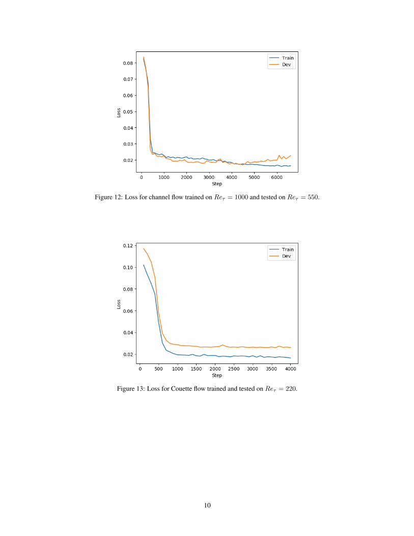
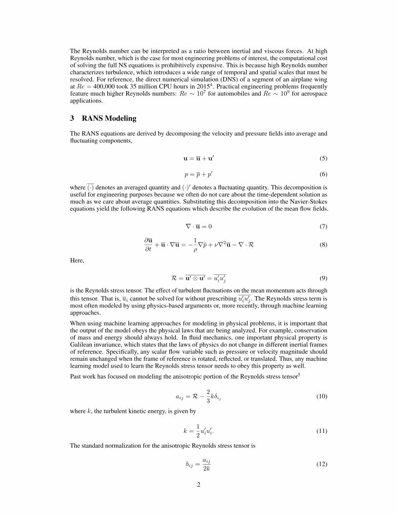
Figure 12: Loss for channel flow trained on Reτ = 1000 and tested on Reτ = 550.

Figure 13: Loss for Couette flow trained and tested on Reτ = 220.

10

Figure 14: Loss for Couette flow trained and tested on Reτ = 500.

Figure 15: Loss for Couette flow trained on Reτ = 220 and tested on Reτ = 500.

11

Figure 16: Loss for Couette flow trained on Reτ = 500 and tested on Reτ = 220.

Figure 17: Mean velocity profiles of all flows studied.

12

Figure 18: Mean turbulent kinetic energy of all flows studied.

13

10 Appendix B: Background on Fluid Flows

i. Channel flow

Channel flow is a pressure-driven flow of a fluid through a rectangular duct of height 2h in whichthe mean flow is predominantly in the axial direction (x), and the mean velocity is varying mainlyin the wall-normal (y) direction. The extent of the channel in the spanwise (z) direction is largesuch that the flow is statistically independent of z. Near the entry of the channel (x = 0), there isa flow-development region in which the physics are complicated. However, sufficiently far awayfrom the inlet, flow statistics will no longer vary with x. Computationally, the fully developed flow isrepresented by implementing periodic boundary conditions in the x and z directions.

Note that the convention in fluid dynamics is that x = x1, y = x2, and z = x3 are used practicallyinterchangeably. Similarly, the velocity in the x direction can be u or u1, velocity in the y direction isv or u2, and velocity in the z direction is w or u3.

The governing equations for the mean flow are

νdu

dy= u′v′ +

τwρ

(1− y

h

)(14)

where

τw = ρνdu

dy

∣∣∣∣y=0

. (15)

The boundary conditions at the wall are no-slip, meaning that the fluid velocity is equal to the velocityof the walls. In this case, the fluid velocity is zero at the walls.

Figure 19: Channel flow schematic

ii. Couette flow

Couette flow is the flow of a fluid between two surfaces, one of which is impulsively started andmoving tangentially relative to the other. The relative motion of the surfaces imposes a shear stresson the fluid and induces the flow. After the initial start up period, the flow becomes statisticallystationary in time and independent of x and z.

dv

dy= 0 (16)

νdu

dy= u′v′ + τw (17)

There are two key differences between channel flow and Couette flow. The first is that channel flowis driven by a pressure gradient, while Couette flow is driven by the shear induced by the velocity ofthe moving surface. The second difference is that, by the no-slip boundary condition, the velocity ofthe fluid on the upper wall of Couette flow is equal to the moving wall’s velocity. This is in contrastto channel flow, where the upper wall is stationary.

14

Figure 20: Couette flow schematic

iii. Superhydrophobic surface

A superhydrophobic surface is one in which a thin air film is formed between the solid surface andthe fluid it is immersed in. This air film reduces the viscosity at the wall and leads to significant dragreduction at the wall.

This drag reduction is commonly modelled as a slip boundary condition11, 12, 13, 14. Instead of theno-slip condition described in the channel and Couette flows, a slip boundary condition at the wallmeans that

u(y = 0) = bdu

dy

∣∣∣∣y=0

(18)

w(y = 0) = bdw

dy

∣∣∣∣y=0

(19)

where b is some fixed slip length. Note that the velocity gradient involved in the boundary conditionis a local velocity gradient, not a mean velocity gradient.

Figure 21: Slip boundary condition schematic

The SHS data used in our analysis follows the same governing equations as channel flow. The onlydifference is the boundary condition at y = 0 and y = 2h. In our data, the nondimensionalized sliplength is b+ = 9.

v. Tensor invariants

It is shown in Pope6 that the most general representation of the anisotropic Reynolds stress tensor interms of the mean strain-rate and rotation rate tensors is

bij(Sij , Rij) =

10∑n=1

G(n)(λ1, ..., λ5)T(n)ij (20)

where λi are scalar invariants and Tij are the tensor basis.

15

T (1) = S T (6) = R2S + SR2 − 2

3Tr(SR2

)I (21)

T (2) = SR− RS T (7) = RSR2 − R2SR

T (3) = S2 − 1

3Tr(S2)I T (8) = SRS2 − S2RS

T (4) = R2 − 1

3Tr(R2)I T (9) = R2S2 + S2R2 − 2

3Tr(S2R2

)I

T (5) = RS2 − S2R T (10) = RS2R2 − R2S2R

where

S =k

2ε

(∇u + (∇u)T

)(22)

R =k

2ε

(∇u− (∇u)T

). (23)

The invariants are

λ1 = Tr(S2), λ2 = Tr

(R2), λ3 = Tr

(S3), λ4 = Tr

(R2S

), λ5 = Tr

(R2S2

). (24)

For the case of channel flow and Couette flow, the structure of S and R are such that λ3 and λ4 areidentically zero. It was important to remove these scalar invariants from the neural network model,otherwise division by zero was encountered. For the SHS channel, all five scalar invariants are active.

16

References1 Steven L Brunton, Bernd R Noack, and Petros Koumoutsakos. Machine learning for fluid mechanics.

Annual Review of Fluid Mechanics, 52:477–508, 2020.

2 J Nathan Kutz. Deep learning in fluid dynamics. Journal of Fluid Mechanics, 814:1–4, 2017.

3 Julia Ling, Andrew Kurzawski, and Jeremy Templeton. Reynolds averaged turbulence modellingusing deep neural networks with embedded invariance. Journal of Fluid Mechanics, 807:155–166,2016.

4 Seyed Mohammad Hosseini, Ricardo Vinuesa, Philipp Schlatter, Ardeshir Hanifi, and Dan SHenningson. Direct numerical simulation of the flow around a wing section at moderate reynoldsnumber. International Journal of Heat and Fluid Flow, 61:117–128, 2016.

5 Stephen B Pope. Turbulent flows, 2001.

6 SB Pope. A more general effective-viscosity hypothesis. Journal of Fluid Mechanics, 72(2):331–340, 1975.

7 JC Del Alamo and J Jimenez. Direct numerical simulation of the very large anisotropic scales in aturbulent channel. Center for Turbulence Research Annual Research Briefs, 2001.

8 Juan C Del Alamo and Javier Jiménez. Spectra of the very large anisotropic scales in turbulentchannels. Physics of Fluids, 15(6):L41–L44, 2003.

9 Juan C Del Alamo, Javier Jiménez, Paulo Zandonade, and Robert D Moser. Scaling of the energyspectra of turbulent channels. Journal of Fluid Mechanics, 500:135, 2004.

10 Rui Fang, David Sondak, Pavlos Protopapas, and Sauro Succi. Neural network models for theanisotropic reynolds stress tensor in turbulent channel flow. Journal of Turbulence, 21(9-10):525–543, 2020.

11 Eric Lauga and Howard A Stone. Effective slip in pressure-driven stokes flow. Journal of FluidMechanics, 489:55, 2003.

12 Robert J Daniello, Nicholas E Waterhouse, and Jonathan P Rothstein. Drag reduction in turbulentflows over superhydrophobic surfaces. Physics of Fluids, 21(8):085103, 2009.

13 A Busse and ND Sandham. Influence of an anisotropic slip-length boundary condition on turbulentchannel flow. Physics of Fluids, 24(5):055111, 2012.

14 Jongmin Seo and Ali Mani. On the scaling of the slip velocity in turbulent flows over superhy-drophobic surfaces. Physics of Fluids, 28(2):025110, 2016.

17