Verdon, J., & Budge, J. (2018). Examining the Capability of StatisticalModels to Mitigate Induced Seismicity during Hydraulic Fracturing ofShale Gas Reservoirs. Bulletin of the Seismological Society ofAmerica, 108(2), 690-701. https://doi.org/10.1785/0120170207

Peer reviewed versionLicense (if available):UnspecifiedLink to published version (if available):10.1785/0120170207

Link to publication record in Explore Bristol ResearchPDF-document

This is the author accepted manuscript (AAM). The final published version (version of record) is available onlinevia GSA at https://pubs.geoscienceworld.org/ssa/bssa/article/528918/Examining-the-Capability-of-Statistical-Models-to . Please refer to any applicable terms of use of the publisher.

University of Bristol - Explore Bristol ResearchGeneral rights

This document is made available in accordance with publisher policies. Please cite only thepublished version using the reference above. Full terms of use are available:http://www.bristol.ac.uk/pure/user-guides/explore-bristol-research/ebr-terms/

1

Examining the capability of statistical models to 1

mitigate induced seismicity during hydraulic 2

fracturing of shale gas reservoirs 3

James P. Verdon1*, Jessica Budge2 4

1. School of Earth Sciences, University of Bristol, Wills Memorial Building, Queen’s 5

Road, Bristol, U.K., BS8 1RJ. 6

2. Nexen Energy ULC, 801 7th Avenue SW, Calgary, AB, Canada, T2P 3P7. 7

8

* Corresponding Author. Email: James.Verdon@bristol.ac.uk, Tel: 0044 117 331 9

5135. 10

11

12

13

2

ABSTRACT 14

Injection into the subsurface is carried out by industry for a variety of reasons: storage of waste-water; 15

enhanced oil recovery; and for hydraulic fracture stimulation. By increasing subsurface pressures, 16

injection can trigger felt seismicity (i.e. of sufficient magnitude to be felt at the surface) on pre-existing 17

faults. As the number of cases of felt seismicity associated with hydraulic fracturing has increased, 18

strategies for mitigating induced seismicity are required. However, most hydraulic stimulation 19

activities do not induce felt seismicity. Therefore a mitigation strategy is required that is capable of 20

differentiating the “normal” case from “abnormal” cases that trigger larger events. In this paper we 21

test the ability of statistical methods to estimate the largest event size during stimulation, applying 22

these approaches to two datasets collected during hydraulic stimulation in the Horn River Shale, 23

British Columbia, where hydraulic fracturing was observed to reactivate faults. We apply these 24

methods in a prospective manner: using the microseismicity recorded during the early phases of a 25

stimulation stage to make forecasts about what will happen as the stage continues. We do so to put 26

ourselves in the shoes of an operator or regulator, where decisions must be taken based on data as it is 27

acquired, rather than a post hoc analysis once a stimulation stage has been completed. We find that the 28

proposed methods can provide a reasonable forecast of the largest event to occur during each stage. 29

This means that these methods can be used as the basis of a mitigation strategy for induced seismicity. 30

31

3

INTRODUCTION 32

Hydraulic Fracturing-Induced Seismicity 33

Any human activity that alters the stress state in the Earth’s crust has the potential to induce 34

seismic activity. Induced seismicity has been associated with: mining (e.g., Li et al., 2007); 35

impoundment of reservoirs (e.g., Gupta, 1985); conventional oil and gas extraction (e.g., 36

Segall, 1989); and subsurface fluid injection, whether for hydraulic fracturing (e.g., Bao and 37

Eaton, 2016), disposal of waste fluids (e.g., Keranen et al., 2013), Carbon Capture and 38

Storage (e.g., Stork et al., 2015), or geothermal energy (e.g., Häring et al., 2008). 39

It has been conclusively demonstrated that injecting fluids into the subsurface can trigger 40

seismicity, where increased pore-fluid pressures lead to the activation of critically-stressed 41

faults (e.g., Raleigh et al., 1976). However, it should be noted that the overwhelming majority 42

of such operations are not thought to cause earthquakes. Nevertheless, as the above practices 43

have increased in scale and become more widespread, the issue of injection-induced 44

seismicity has grown in significance. 45

While much of the recent focus has been on waste-water disposal, several cases of hydraulic 46

fracturing-induced seismicity (HF-IS) have been identified (e.g., B.C. Oil and Gas 47

Commission 2012, 2014; Clarke et al. 2014; Friberg et al., 2014; Darold et al., 2014; Skoumal 48

et al., 2015; Schultz et al. 2015a,b; Atkinson et al., 2016; Bao and Eaton, 2016; Wang et al., 49

2016). It is vital that our understanding of HF-IS improves, such that industrial operators are 50

capable of mitigating against triggering seismic activity. However, for many of these case 51

examples monitoring arrays were not deployed until after large events had occurred, or 52

available monitoring arrays consisted solely of regional networks, where the nearest station 53

may have been many km from the site. This means that there is often little useful data that can 54

be used to study the processes that happened in the lead-up to these events, and thereby what 55

mitigation steps might have been possible. 56

4

The number of cases of HF-IS is very small when compared to the overall number of wells 57

that have been hydraulically stimulated. As such, any mitigation scheme should be capable of 58

quickly differentiating the “normal case”, where hydraulic fracturing does not cause fault re-59

activation leading to larger events, from the “abnormal case” where large events may be 60

triggered, and therefore where mitigating strategies, such as reducing injection volumes or 61

ceasing injection altogether, may be necessary. 62

Mitigation of HF-IS 63

At present, where regulations pertaining to HF-IS have been applied, they have taken the 64

form of Traffic Light Schemes (TLSs), whereby operators take actions based on the 65

magnitude of events induced during operations. These schemes have the advantage of being 66

relatively simple to administer, and can be understood by the public. However, there are 67

somewhat reactive in their nature (as opposed to proactive): an operational response is 68

required, such as reducing or stopping injection, only after an event of a given size has 69

occurred. 70

The purpose of this paper is not to argue against the use of TLSs, which can play a useful role 71

in the regulation of HF-IS. However, it is our view that, in addition to complying with TLS 72

regulations, operators should seek to mitigate induced seismicity in a more proactive manner. 73

If nothing else, operators will wish to ensure that they remain within the specified TLS 74

thresholds during their operations, since reaching “red lights” entails the imposition of 75

operational constraints, and may also affect operator reputation and confidence with the 76

public. 77

To take a proactive approach to HF-IS, operators must develop the capacity to model their 78

activities, allowing them to make forecasts about the HF-IS that may occur as their operations 79

continue. In the broadest sense, two types of modelling approach are available: physical and 80

statistical. Physical models aim to simulate the processes that occur during hydraulic 81

stimulation, usually using numerical methods such as finite elements (e.g. Maxwell et al., 82

2015), discrete elements (e.g., Yoon et al., 2014), rate and state approaches based on 83

5

modelled stress changes (e.g., Hakimhashemi et al., 2014), or by resolving modelled stress 84

changes onto pre-existing fault/fracture networks (e.g., Verdon et al., 2015). However, such 85

models often require extensive site characterisation to identify and characterise both nearby 86

faults and the local stress state. Such models also come with a significant number of free 87

parameters that must be “tuned” to provide a reasonable representation of reality. As such 88

they are better suited for understanding the physical processes that have occurred at a site a 89

posteriori. For hydraulic fracturing operators who might be required to manage induced 90

seismicity in real time at a significant number of active well sites, simple models with a 91

relatively small number of free parameters are required. In this respect, statistical models 92

become more favourable. 93

Statistical approaches seek to characterise the observed seismic event population via a 94

statistical model, usually the Gutenberg and Richter (1944) (G-R hereafter) distribution. Such 95

a model can then be extrapolated to estimate the event population that is expected to have 96

occurred by the end of the injection period. Several such models have been proposed, for 97

example: Shapiro et al. (2010); McGarr (2014); Hallo et al. (2014); and van der Elst et al. 98

(2016). 99

These models are similar in their underlying assumptions: event magnitudes can be 100

characterised by the G-R distribution, and the rate of seismicity is linked in some way to the 101

injection volume. This relationship is then extrapolated based on recorded seismicity during 102

the early stages of injection to estimate what the resulting event population would be once the 103

total volume has been injected. From this estimated population, the largest event size can be 104

forecast. These models have the advantage that they require only a few parameters, which can 105

be measured as operations progress. This makes them better-suited for the task of providing a 106

priori mitigation of induced seismicity. 107

While these models have been tested at several sites (e.g. Hallo et al., 2014; Hajati et al., 108

2015), the crucial aspect investigated in this paper is that we seek to apply these methods in a 109

prospective manner (e.g. Langenbruch and Zoback, 2016). We do not apply these models 110

6

using the overall event population that has been acquired during hydraulic stimulation in a 111

post hoc manner. Instead, we put ourselves into the shoes of an operator or regulator, where 112

forecasts must be made using only the data that has been acquired prior to a given point in 113

time. Evidently, the underlying assumption for these methods is that the parameters used to 114

characterise the seismicity as a function of injection volume remain unchanged during a given 115

operation. 116

We apply these methods to two datasets collected during hydraulic stimulation in the Horn 117

River Shale. These multi-well, multi-stage sites were monitored using downhole 118

microseismic arrays, producing very high quality datasets. These datasets are described in the 119

following section, after which we describe the methods of Shapiro et al. (2010) and Hallo et 120

al. (2014) in greater detail, and apply them to the datasets. 121

DATASETS 122

In our case example we examine microseismic datasets from two multi-well, multi-stage 123

hydraulic fracturing treatments conducted in the Horn River Shale formation in British 124

Columbia, Canada. The pads from which the two sets of wells were drilled are approximately 125

7km apart from each other. In the following we refer to the two datasets as HR1, which was 126

completed in 2011, and HR2, which was completed in 2013. These datasets were provided by 127

the operating company: they are proprietary and cannot be released to the public. 128

HR1 Microseismic Data 129

A total of 9 horizontal wells were drilled from the HR1 pad. A total of 146 stages were 130

stimulated, with between 15 – 18 stages per well. Microseismic data was recorded by arrays 131

of up to 100 3-component geophones placed in boreholes adjacent to those being stimulated 132

(in both the vertical and horizontal sections of the wells). The positions of the geophones 133

were varied as stimulation progressed along the wells, in at least 21 configurations. 134

7

Data were provided from 76 of the stages, consisting of a total of 140,100 events. These were 135

the stages closest to the heels of the wells, and therefore closest to the monitoring arrays, 136

where the best quality microseismic data could be gathered. Events were located by inverting 137

picked P- and S-wave arrival times through a layered, anisotropic velocity model. A map and 138

cross-section of the HR1 microseismic events are shown in Figure 1. Event magnitudes were 139

calculated by fitting an idealised source model to the event displacement spectra to determine 140

the seismic moment (e.g., Stork et al., 2014). Throughout this paper, when referring to 141

“magnitude” our implication is moment magnitude, MW. In both cases this processing of the 142

data was performed by a service provider, ESG Solutions. 143

HR2 Microseismic Data 144

A total of 10 wells were drilled from the HR2 pad. 237 stages were stimulated, with between 145

23 – 24 stages per well. Microseismic data was recorded by an array of 96 3-component 146

geophones placed in 3 adjacent boreholes. Data was provided from 119 stages, consisting of 147

92,700 events. As with the HR1 pad, data was provided for the stages nearest to the heels of 148

the wells, where they are in closest proximity to the monitoring array (and therefore are 149

expected to provide the best quality data). A map and cross-section of the HR2 events are 150

shown in Figure 2. 151

In both case studies, examination of event locations reveals evidence for the interaction 152

between hydraulic fracturing and faults in the form of planar features extending downwards 153

into the underlying Keg River limestone formation. At HR1, the largest event has a 154

magnitude of MW = 1.3, while at HR2 the largest event has a magnitude of MW = 0.5. In both 155

cases, these magnitudes are larger than what is typically observed when hydraulic fractures 156

propagate through shale gas reservoirs, where magnitudes are generally less than 0 (e.g., 157

Maxwell et al., 2010). 158

USING EVENT POPULATION STATISTICS TO FORECAST THE LARGEST 159

EVENT SIZE 160

8

In the following sections, we refer to MOMAX as the largest magnitude event observed during a 161

particular stage, and MMMAX as the expected largest magnitude as estimated by a modelling 162

strategy. Ideally, modelling strategies should aim to produce conservative estimates of MMMAX, 163

such that MOMAX ≤ MM

MAX. Here we examine the abilities of two published methods, Shapiro 164

et al. (2010) and Hallo et al. (2014), to forecast MMMAX during hydraulic stimulation. 165

Seismogenic Index, Shapiro et al. (2010) 166

Shapiro et al. (2010) define the Seismogenic Index, SI as 167

𝑆" = log'((*+ ,-+

) + 𝑏𝑀, (1) 168

where Nt(M) is the number of events that have occurred at time t that are larger than a given 169

magnitude M, b is the G-R b-value for the observed event magnitude distribution (EMD), and 170

Vt is the cumulative volume injected up until this time (note that Shapiro et al. (2010) use S to 171

denote the seismogenic index: we use SI instead to differentiate with other uses of S 172

elsewhere in this paper). Assuming that the number of events induced per unit volume 173

injected does not change, then SI will be constant: constant SI has been observed by Dinske 174

and Shapiro (2013) and van der Elst et al. (2016) for a wide range of cases studies. Shapiro et 175

al. (2010) show that, in such an instance, if the occurrence of individual events can be treated 176

as an independent Poisson process, then the probability that an event larger than M does not 177

occur if a total volume VT is injected can be calculated as 178

ℙ = exp −𝑉8. 10<=>?, . (2) 179

Re-arranging this equation, we arrive at a forecast for the size of event that will not be 180

exceeded, given a confidence level c: 181

𝑀,@A, = 𝑆" − log

>CD(E)-F

/𝑏. (3) 182

In order to provide a mitigation strategy, we are interested in establishing an upper bound for 183

MMAX, i.e., to establish what size of earthquake will not occur (or is unlikely to occur). 184

9

Therefore, for the entirety of this study we consider the upper bound of the distribution 185

described by Shapiro et al. (2010), setting c = 0.95. 186

Seismic Efficiency, Hallo et al. (2014) 187

McGarr (2014) proposed that the cumulative seismic moment released during injection, SMO, 188

is determined by the total cumulative volume of fluid injected: 189

Σ𝑀I = 2𝜇𝑉8, (4) 190

where µ is the rock shear modulus. However, this equation can be considered as a worst-case 191

scenario, where all the strain induced by a volume change is released as seismic energy. In 192

reality, much of the deformation induced by injection will be released aseismically. Hallo et 193

al. (2014) therefore define a seismic efficiency ratio, SEFF, which describes the ratio of 194

observed cumulative moment release to the theoretical maximum given by µVT. Equation 3 is 195

thereby modified to: 196

Σ𝑀I = 𝑆LMM𝜇𝑉8, (5) 197

where SEFF can be estimated at a given time from the cumulative moment release and the 198

cumulative injected volume up until this time. 199

For a given cumulative seismic moment release, size of the largest event will be determined 200

by the b value. Hallo et al. (2014) show that SMO can be related to the b value, and the largest 201

event detected, MMMAX, and the minimum magnitude of completeness, MMIN: 202

Σ𝑀I =?.'(N.'(O.P

'.Q>?10 ,RST

R '.Q>? − 10 ,R=U '.Q>? , (6) 203

where 204

𝑎 = 𝑏𝑀,@A, − log 10?W − 10>?W , (7) 205

and d is the probabilistic half-bin size defined around MMMAX, as described by Hallo et al. 206

(2014). Based on equation 5, we can determine the total expected SMO based on the observed 207

seismic efficiency SEFF and the planned total injection volume VT. Once we have estimated 208

10

SMO, we invert equations 6 and 7 to forecast MMMAX based on the observed b values. 209

Essentially, MMMAX is a function of the seismic efficiency, which describes how much seismic 210

moment is released per unit volume injected, and the b value, which describes whether this 211

seismic moment is released as a few large events or as many small events. 212

Whereas the Shapiro et al. (2010) SI method provides a probability distribution for MMAX 213

(Equation 3), the Hallo et al. (2014) method provides a single estimate for MMMAX based on 214

the observed (or forecast) b and SEFF values. As such, assuming the Hallo et al. method is a 215

true representation of the induced seismicity, random variability alone would mean that the 216

actual MOMAX value would be larger than the model for half the cases. As described above, our 217

aim is to establish conservative MMMAX values, whereby we have confidence that no events 218

larger than MMMAX will occur. Therefore we require a value based on equations 6 and 7 that 219

also takes into account uncertainties inherent in the approach. 220

To do this we consider synthetic, stochastically generated event populations. By randomly 221

sampling from a G-R distribution, we generate event populations with a given b value and 222

SMO chosen randomly from 0.8 < b < 3.5 and 9 < log'( Σ𝑀I < 14. We then compare the 223

largest sampled event (which we refer to as the “synthetic MOMAX”) with that forecast from the 224

given b and SMO values using equations 6 and 7 (the “forecast MMMAX”). Our results for 1,000 225

such realisations are shown in Figure 3. We find that for 98% of model realisations, the 226

forecast value of MMMAX is within 0.5 magnitude units of the synthetic MO

MAX. Because we are 227

primarily concerned with setting a conservative envelope that is not exceeded, in the 228

following sections we take as MMMAX the value computed using the Hallo et al. method 229

(equations 6 and 7) + 0.5. 230

There is currently some debate as to whether there really is a link between injection volume 231

and the rate and/or size of induced earthquakes (e.g. Atkinson et al., 2016; van der Elst et al., 232

2016). This debate stems from fundamental questions as to the nature of rupture mechanics 233

during induced seismicity. Gischig (2015) describes two end-members for rupture behaviour. 234

In the first case rupture may initiate within the zone of increased pressure, but uncontrolled 235

11

rupture can continue along faults outside of this zone, releasing tectonically-accumulated 236

strain energy. Event size will be therefore determined by tectonic factors such as fault 237

dimensions and in situ stress conditions. In the second case the rupture is spatially limited to 238

the zone of increased pore pressure, in which case the injection volume places an a priori, 239

deterministic limit on the maximum event size. 240

The second case, where the injection volume places a deterministic limit on event size, is 241

often characterised by the McGarr (2014) limit (Equation 4). However, observations of events 242

that appear to breach this limit (e.g., Atkinson et al., 2016) indicate that, at least in certain 243

cases, the first of the Gischig (2015) end-members applies. Therefore an a priori 244

deterministic limit on event size cannot be assumed based on injection volume. 245

However, in our approach there is no requirement that SEFF ≤ 1, and therefore there is no a 246

priori deterministic limit to event size. If SEFF > 1, this indicates that the cumulative moment 247

released is larger than the strain energy introduced by injection, and therefore that tectonically 248

accumulated strain energy is also being released. Equation (5) requires simply that there is 249

proportionality between VT and SMO, where SEFF is to be determined by observation for a 250

given site. Van der Elst (2016) examined a range of case studies to investigate whether the 251

number of earthquakes induced during injection is proportional to injection volume, and 252

found strong evidence that this was indeed the case, with the implication that the event 253

nucleation rate is controlled by the injection volume. If b values are constant, then this 254

implies that the cumulative moment release will also be proportional to injection volume. 255

Application to microseismic data 256

To compute b values we use the maximum likelihood approach described by Aki (1965). To 257

estimate MMIN, we follow the method described by Clauset et al. (2009) to assess the quality 258

of fit between the observed EMD and the G-R relationship using a Kolmogorov-Smirnov 259

test, choosing as MMIN the smallest magnitude at which the null hypothesis (that the observed 260

distribution can be modelled by the G-R relationship) is not rejected at a 10% significance 261

12

level. Fitting a G-R relationship to an observed EMD can be unreliable for low event 262

numbers. Therefore we require a minimum of 50 events with magnitudes larger than MMIN for 263

a reliable measurement. This means that our approach will only provide an estimate for 264

MMMAX once sufficient microseismic events have occurred. 265

Figure 4 shows an example of how we apply these methods to the microseismic datasets. 266

Plots for every stage are available in the supplementary materials. We proceed at intervals of 267

120 seconds. After each interval has elapsed, we re-calculate the b, SEFF, and SI parameters 268

based on the total volume injected and the events recorded up until this time. We then use 269

equations 3, 6 and 7 to estimate, using the Shapiro et al. (2010) and Hallo et al. (2014) 270

methods, the expected value of MMMAX given the injection volume that is planned to take place 271

during the next 120s interval. 272

In the lower panel of Figure 4, we plot the measured values of b, SEFF, and SI with time. In the 273

upper panel of Figure 4 we compare the resulting forecasts of MMMAX with observed event 274

magnitudes. We note that in the example shown in Figure 4, the forecast largest event size 275

stabilizes at a value of approximately MMMAX = 0.2 within 40 minutes of the start of injection. 276

This is slightly larger than the largest observed event, which has a magnitude of MOMAX = 0.0 277

and occurs 140 minutes after the start of injection. 278

In the following sections we compare MOMAX with the value of MM

MAX at the time that the 279

largest event occurred. We also compare MOMAX with MM

MAX at a time 60 and then 30 minutes 280

before the largest event occurred. We do this to identify the capacity of such methods to 281

provide an opportunity for mitigation by giving an operator sufficient warning to alter (or 282

cease) their stimulation program. 283

Before considering the results of our method as applied to all stages of both datasets, we note 284

several features from Figure 4. Firstly, we note the similarity between the two curves for SI 285

and log10(SEFF). This is to be expected given how the two parameters are defined. If MMIN is 286

used as the “M” term in equation 3, then the difference SI – log10(SEFF) will be given by: 287

13

𝑆" − log 𝑆LMM = log(𝑁Y(𝑀,"*)/𝑉Y) + 𝑏𝑀,"* − log Σ𝑀I/𝜇𝑉Y . (8) 288

Rearranging this equation, and substituting SMO = Nt<MO>, where <MO> is the mean moment 289

release per event, we get 290

𝑆" − log 𝑆LMM = 𝑏𝑀,"* − log 𝑀I /𝜇 . (9) 291

In the case studies presented here, MMIN is typically approximately -1.5, b is typically 2, <MO> 292

is typically of the order 107 Nm (equivalent to a magnitude of approximately -1) and we 293

approximate the shear modulus as µ = 20x109 Pa. Hence the similarity in values between SI 294

and log10(SEFF). We also note that the values of MMMAX computed by the two methods are 295

similar. This gives us confidence that both independent methods are providing similar results. 296

RESULTS 297

Before showing the results using the two methods described above, in Figure 5 we compare 298

the observed values for MOMAX for each stage with the values of MM

MAX forecast using the 299

McGarr (2014) equation MMMAX = µVT. We do this primarily to demonstrate that there does 300

not appear to be any correlation between the observed MOMAX of each stage and the volume 301

injected at the time of occurrence of each event. We also note that the observed magnitudes 302

are far smaller than those estimated by the McGarr (2014) equation. 303

In Figure 6 we compare the observed and forecast MMAX values using the Hallo et al. (2014) 304

method. As per Figure 4, we compare the forecast MMMAX values at the time that the largest 305

event occurred, but also compare the forecast MMMAX values 30 and 60 minutes before the 306

occurrence of the largest event. In Figure 7 we do the same for the Shapiro et al. (2010) 307

method. 308

We note several features from these results. Firstly, as required, in general MMMAX ≥ MO

MAX for 309

almost every stage. Not only this, but stages that produced smaller events have smaller values 310

of MMMAX, id est there is clear correlation between MM

MAX and MOMAX. This is encouraging, as 311

it implies that these methods do have some forecasting power, unlike the results provided by 312

14

the McGarr (2014) approach shown in Figure 5. This correlation is present even for the T – 313

60mins measurements, implying that these methods are capable of identifying stages that may 314

induce larger events a significant period of time before such events occur. 315

There is only 1 stage, at HR2, where both the Shapiro et al. (2010) and Hallo et al. (2014) 316

methods significantly underestimate MOMAX. We note that this stage had only 131 events in 317

total, making it one of the smallest stages in terms of the number of events. The robustness of 318

statistical techniques such as these will be dependent on the number of events sampled, so it 319

is perhaps unsurprising that stages with fewer events might produce less reliable results. 320

DISCUSSION 321

Do seismicity parameters vary during injection stages? 322

The models we use to forecast MMMAX are entirely statistical, and do not incorporate any 323

geological information. The major advantage of these statistical approaches is that they are 324

relatively simple to use (requiring only that the volume injected, and the number and 325

magnitude of seismic events can be measured). The principal assumption that underpins this 326

type of approach is that both b, SEFF and/or SI will remain consistent throughout the injection 327

period. It is by no means clear that this will always be the case. 328

These parameters might be affected by a range of factors including: the in situ stress 329

conditions; the lithology of the rock through which hydraulic fractures are propagating; and 330

the presence of pre-existing fracture networks and/or faults. Generally speaking, the volume 331

of rock influenced by injection increases as the pressure front moves out from the injection 332

well. Therefore, the pressure pulse induced by injection may begin to act on different layers 333

and/or structures as injection continues. It is easy to imagine scenarios where a growing 334

hydraulic fracture intersects with a pre-existing fault, or propagates into an under- or 335

overlying layer that is more seismogenic, resulting in a change in the rate of seismicity and/or 336

b value. 337

15

The key question then becomes whether such changes are rapid, or whether there will be a 338

more gradual evolution. If the seismicity changes suddenly then larger events may occur that 339

cannot be anticipated based on the preceding microseismicity. It would therefore be very 340

difficult for an operator to mitigate induced seismicity, as larger events would occur “out of 341

the blue”. In contrast, if such changes occur relatively gradually then an operator may be able 342

to identify an increase in the seismicity rate, or a decrease in the G-R b-value, that would 343

indicate an increasing probability of a larger event occurring. If closely monitored, this might 344

allow an operator to take appropriate mitigating action (reducing pumping rates and/or 345

pressures, or indeed ceasing to pump altogether). 346

Incidentally, this assumption is also implicit in existing schemes that are used to mitigate 347

induced seismicity, such as TLSs, although this assumption is rarely stated explicitly. If large 348

events are triggered immediately when a HF intersects a fault, then TLSs will be ineffective, 349

because an event that is much larger than the red-light threshold could occur without any 350

prior TLS-based mitigation actions having been taken. In contrast, if there is a more gradual 351

build-up of seismicity upon intersection between a hydraulic fracture and a fault, then the 352

amber and red lights will progressively be triggered, and the appropriate mitigation steps 353

taken. 354

We note that both Dinske and Shapiro (2013) and van der Elst et al. (2016) have observed 355

remarkably constant values of SI during fluid injection, across a wide variety of settings 356

including hydraulic fracturing, stimulation of geothermal reservoirs, and during wastewater 357

disposal. There are also sound physical reasons to expect a gradual increase in seismic 358

magnitudes as a hydraulic fracture impinges on a fault, as opposed to a sudden “jump”. When 359

a fracture first meets a fault, both the area of the fault affected, and the volume of fluid 360

injected into the fault will be small. As such, we might expect the initial events to be smaller. 361

As injection continues, the area of the fault affected will increase, as will the volume of fluid 362

injected into it, which would be expected to increase the event magnitudes as injection 363

continues. 364

16

This assumption is borne out in the results we present here, most notably in the fact that the 365

forecast MMMAX values tend to anticipate the observed largest events by at least 60 minutes 366

(Figures 6 and 7). It is also apparent when the evolution of these parameters is examined in 367

detail during each stimulation stage (see supplementary material). The implication is that 368

large induced events do not occur “out of the blue”, but are accompanied by a build-up in 369

seismicity as the stimulation impinges on a pre-existing fault. 370

Strategy for Mitigation of Induced Seismicity 371

Based on the above results, we suggest the following strategy for the mitigation of induced 372

seismicity. Prior to the start of operations, an acceptable threshold for MMMAX is set, based on 373

the vulnerability of nearby populations, buildings and infrastructure to seismic activity, and 374

the expected ground motion that would be caused by events of a given size. 375

In this case, we arbitrarily set our thresholds as MMMAX > 1. Given the relative lack of 376

buildings, local populations or infrastructure near to this site, this is a relatively conservative 377

threshold, but nevertheless affords a clear demonstration of the approach. Because the results 378

for the Hallo et al. (2014) method show a tighter correlation between MMMAX and MO

MAX (c.f. 379

Figures 6 and 7), we use this approach as our preferred method to compute MMMAX. If MM

MAX 380

exceeds this threshold during a stage, then mitigating actions should be taken. In this case we 381

suggest that the mitigating action would be to cease injection and move on to the next stage. 382

Based on our results, we divide the stages into 3 categories: stages where the MMMAX > 1 383

threshold is never reached and therefore no mitigation action is indicated (Figure 8a,b); stages 384

where the MMMAX > 1 threshold is reached only after the occurrence of the largest observed 385

event (Figure 8c,d); and stages where the MMMAX > 1 threshold is reached before the 386

occurrence of the largest event (Figure 8e,f). 387

The first category of stages, where the MMMAX > 1 threshold was not exceeded at any time, is 388

represented in Figure 8a. An example of such a stage is shown in Figure 8b. 159 out of 195 389

total stages (82%) fall into this category. The circles in Figure 8a show the largest event to 390

17

occur in each of these stages: the largest event to occur in a stage where the MMMAX > 1 391

threshold was not reached had a magnitude of MW = 0.4. 392

The second category of stages is where the MMMAX > 1 threshold was exceeded, but only after 393

the occurrence of the largest event (Figure 8c). An example of such a stage is shown in Figure 394

8d: in this stage the largest event, which has a magnitude of MOMAX = 0.58, occurs after 395

approximately 1 hour. The MMMAX > 1 threshold is reached after 2 hours of injection. Because 396

the threshold is reached after the occurrence of the largest event, any mitigation steps that 397

might have been taken would not affect the size of largest event to occur during these stages. 398

A total of 16 stages (8%) fall into this category, and MOMAX for each of these stages is 399

depicted in Figure 8c. The largest magnitude event to occur during these stages had a 400

magnitude of MW = 0.88. 401

The third category of stages is where the MMMAX > 1 threshold was exceeded prior to the 402

occurrence of the largest event. An example of such a stage is shown in Figure 8f: in this 403

stage the MMMAX > 1 threshold is reached after approximately 1 hour of injection. This is over 404

2.5 hours before the occurrence of the largest event, which had a magnitude of MOMAX = 1.24. 405

In other words, the potential for an MW > 1 event is identifiable at a relatively early point 406

during the stage, and it is therefore possible that actions could have been taken that might 407

have mitigated the occurrence of this event. A total of 20 stages (10%) fall into this third 408

category, where the MMMAX > 1 threshold was reached prior to the occurrence of the largest 409

event. These stages are depicted in Figure 8e, where the squares indicate the size of the 410

largest event to occur prior to reaching the MMMAX > 1 threshold, while triangles indicate the 411

eventual largest event to occur. Within this category of stages, three had events with 412

magnitudes larger than MW = 1. However, the largest event to occur before reaching the 413

MMMAX > 1 threshold had a magnitude of MW = 0.65. 414

Overall, we note that for all the stages where the largest event was smaller than MOMAX < 0, no 415

mitigation actions were indicated. For some stages where 0 < MW < 1 mitigation actions were 416

indicated, while in others they were not. For all the stages where the largest event exceeded 417

18

MOMAX > 1, mitigation actions were always indicated prior to the occurrence of these events. 418

The result is that, for our “mitigated” population there are no stages where the largest event 419

exceeds MW > 1. 420

Mitigating actions and post-injection seismicity 421

The major caveat that applied to the results described above is the assumption that ceasing 422

injection can prevent the subsequent larger events from happening. In reality injection was 423

not stopped, and so we cannot know whether cessation of injection during a stage would 424

actually have mitigated the larger events that occurred later in the stage. In other cases of 425

induced seismicity, events have continued with increasing magnitudes even after injection 426

had ceased (e.g., Häring et al., 2008). It is certainly possible that this would have been the 427

case at this site. Therefore it is not possible to definitively conclude that, even if mitigation 428

steps had been taken, further seismicity would not have occurred. Nevertheless, we believe 429

that it is important that operators develop scientific criteria to guide operational decisions 430

with respect to mitigating induced seismicity, and that the results presented here clearly 431

indicate that the methods described in this paper do provide such a basis. 432

CONCLUSIONS 433

We have presented case studies from two sites where microseismic monitoring has imaged 434

pre-existing faults being activated during hydraulic fracturing. We investigate the use of two 435

statistical methods found in the literature (Shapiro et al., 2010; Hallo et al., 2014) to forecast 436

the largest event size that might be expected during a hydraulic fracturing stage. The basis of 437

these two methods is to characterise the rate of seismicity with respect to the injection 438

volume, and thereby extrapolate to an expected event distribution once the planned total 439

volume has been injected. 440

Rather than examining these case studies post hoc, we explore the potential of these methods 441

to work in a prospective manner: at each given time-step we only make use of information 442

19

that is available prior to this time. We do this to put ourselves in the shoes of an operator or 443

regulator, where decisions must be taken in real time as injection proceeds. We find that the 444

proposed methods can forecast the largest event magnitudes with a reasonable degree of 445

accuracy. This enables us to propose a strategy to mitigate HF-IS, whereby alterations to the 446

injection strategy should be made if MMMAX exceeds a given threshold. We show that this 447

strategy may have been able to mitigate the larger events that occurred at our case study sites. 448

The underlying assumption for these methods is that the rate of seismicity with respect to the 449

injection volume will not alter during injection, or that if a fault is encountered, it will evolve 450

gradually, allowing mitigation actions to be taken if real-time monitoring is used. We find 451

that this assumption appears to hold for the datasets considered here. However, further study 452

is required to examine whether this is the case more generally. This highlights the need for 453

good quality seismic monitoring if the science around injection-induced seismicity is to 454

advance. In many of the most well-known case examples, local monitoring arrays were only 455

installed after the largest events had occurred. It is therefore difficult to determine with any 456

certainty what happened in the time leading up to the triggering, and whether an operator 457

could have made observations that in turn might have allowed them to take mitigating 458

actions. 459

The most effective types of monitoring system are either downhole arrays (e.g., Maxwell et 460

al., 2010), as per both case studies in this paper, or Very Large, Very Dense (VLVD) surface 461

arrays, over which data are migrated and stacked (e.g., Chambers et al., 2010). Unfortunately, 462

the costs of these types of deployment are high, and it is unlikely that such systems will be 463

deployed at every injection project. However, novel processing methods using smaller arrays 464

of seismometers placed at the surface (e.g., Skoumal et al., 2015; Verdon et al., 2017) are 465

being used to improve the quality of datasets available. 466

Injection induced seismicity is a growing concern for various industries, and regulators are 467

increasingly requiring operators to deploy monitoring arrays, usually to meet a traffic light 468

scheme requirement of some form. We anticipate that, as more case studies become available, 469

20

our understanding of injection induced seismicity will grow, and our ability to mitigate such 470

events will thereby improve. 471

472

473

Data and Resources 474

The datasets presented in this paper were acquired by the operating company, and are 475

proprietary. Therefore they cannot be released to the public. 476

Acknowledgements 477

The authors would like to thank the operator of these Horn River sites for allowing us to 478

access the data, and to acknowledge ESG Solutions Ltd., the microseismic service provider 479

who processed the dataset. We would also like to thank the sponsors of the Bristol University 480

Microseismicity Project (BUMPS), under whose auspices this work was performed. 481

References 482

Aki, K., 1965, Maximum likelihood estimate of b in the formula log N = a – bM and its 483

confidence limits: Bulletin of the Earthquake Research Institute, University of Tokyo 43, 484

237-239. 485

Atkinson G.M., Ghofrani H., Assatourians K., 2015. Impact of Induced Seismicity on the 486

Evaluation of Seismic Hazard: Some Preliminary Considerations: Seismological Research 487

Letters 86, 1009-1021. 488

Atkinson G.M., Eaton D.W., Ghofrani H., Walker D., Cheadle B., Schultz R., Shcherbakov 489

R., Tiampo K., Gu J., Harrington R.M., Liu Y., van der Baan M., Kao H., 2016. Hydraulic 490

fracturing and seismicity in the Western Canada Sedimentary Basin: Seismological 491

Research Letters 87, 1-17. 492

Bao X., and Eaton D.W., 2016. Fault activation by hydraulic fracturing in western Canada: 493

Science, in press. DOI: 10.1126/science.aag2583 494

21

B.C. Oil and Gas Commission, 2012. Investigation of Observed Seismicity in the Horn River 495

Basin. Accessed from http://www.bcogc.ca/node/8046/download on 23.7.2015. 496

B.C. Oil and Gas Commission, 2014. Investigation of Observed Seismicity in the Montney 497

Trend. Accessed from https://www.bcogc.ca/node/12291/download on 23.7.2015. 498

Chambers K., Kendall J-M., Brandsberg-Dahl S., Rueda J., 2010. Testing the ability of 499

surface arrays to monitor microseismic activity: Geophysical Prospecting 58, 821-830. 500

Clarke H., Eisner L., Styles P., Turner P., 2014. Felt seismicity associated with shale gas 501

hydraulic fracturing: The first documented example in Europe: Geophysical Research 502

Letters 41, 8308-8314. 503

Clauset A., Shalizi C.R., Newman M.E.J., 2009. Power-law distributions in empirical data: 504

Society for Industrial and Applied Mathematics Review 51, 661-703. 505

Darold A., Holland A.A., Chen C., Youngblood A., 2014. Preliminary analysis of seismicity 506

near Eagleton 1-29, Carter County, July 2014: Oklahoma Geological Society Open File 507

Report, OF2-2014. 508

Dinske C. and Shapiro S.A., 2013. Seismotectonic state of reservoirs inferred from magnitude 509

distributions of fluid-induced seismicity: Journal of Seismology 17, 13-25. 510

Friberg P.A., Besana-Ostman G.M., Dricker I., 2014. Characterisation of an earthquake 511

sequence triggered by hydraulic fracturing in Harrison County, Ohio: Seismological 512

Research Letters 85, 1295-1307. 513

Gischig V.S., 2015. Rupture propagation behavior and the largest possible earthquake 514

induced by fluid injection into deep reservoirs: Geophysical Research Letters 42, 7420-515

7428. 516

Gupta H.K., 1985. The present status of reservoir induced seismicity investigations with 517

special emphasis on Koyna earthquakes: Tectonophysics 118, 257-279. 518

Gutenberg B. and Richter C.F., 1944. Frequency of earthquakes in California: Bulletin of the 519

Seismological Society of America 34, 185-188. 520

22

Hajati T., Langenbruch C., Shapiro S.A., 2015. A statistical model for seismic hazard 521

assessment of hydraulic-fracturing-induced seismicity: Geophysical Research Letters 42, 522

10601-10606. 523

Hakimhashemi A.H., Schoenball M., Heidbach O., Zang A., Grünthal G., 2014. Forward 524

modelling of seismicity rate changes in georeservoirs with a hybrid geomechanical-525

statistical prototype model: Geothermics 52, 185-194. 526

Hallo M., Oprsal I., Eisner L., Ali M.Y., 2014. Prediction of magnitude of the largest 527

potentially induced seismic event: Journal of Seismology 18, 421-431. 528

Häring M.O., Schanz U., Ladner F., Dyer B.C., 2008. Characterisation of the Basel 1 529

enhanced geothermal system: Geothermics 37, 469-495. 530

Keranen K.M., Savage H.M., Abers G.A., Cochran E.S., 2013. Potentially induced 531

earthquakes in Oklahoma, USA: Links between wastewater injection and the 2011 MW 5.7 532

earthquake sequence: Geology 41, 699-702. 533

Langenbruch C. and Zoback M.D., 2016. How will induced seismicity in Oklahoma respond 534

to decreased saltwater injection rates? Science Advances 2, e1601542, 535

Li T., Cai M.F., Cai M., 2007. A review of mining-induced seismicity in China: International 536

Journal of Rock Mechanics and Mining Sciences 44, 1149-1171. 537

Maxwell S.C., Rutledge J., Jones R., Fehler M., 2010. Petroleum reservoir characterization 538

using downhole microseismic monitoring: Geophysics 75, A129-A137. 539

Maxwell S.C., Zhang F., Damjanac B., 2015. Geomechanical modeling of induced seismicity 540

resulting from hydraulic fracturing: The Leading Edge 34, 678-683 541

McGarr A., 2014. Maximum magnitude earthquakes induced by fluid injection: Journal of 542

Geophysical Research 119, 1008-1019. 543

Raleigh C.B., Healy J.H., Bredehoeft J.D., 1976. An experiment in earthquake control at 544

Rangely, Colorado: Science 191, 1230-1237. 545

23

Schultz R., Stern V., Novakovic M., Atkinson G., Gu Y.J., 2015a. Hydraulic fracturing and 546

the Crooked Lake sequences: Insights gleaned from regional seismic networks: 547

Geophysical Research Letters 42, 2750-2758. 548

Schultz R., Mei S., Pana D., Stern V., Gu Y.J., Kim A., Eaton D., 2015b. The Cardston 549

earthquake swarm and hydraulic fracturing of the Exshaw Formation (Alberta Bakken 550

play): Bulletin of the Seismological Society of America 105, 2871-2884. 551

Segall P., 1989. Earthquakes triggered by fluid extraction: Geology 17, 942-946. 552

Shapiro S.A., Dinske C., Langenbruch C., 2010. Seismogenic index and magnitude 553

probability of earthquakes induced during reservoir fluid stimulations: The Leading Edge 554

29, 304-309. 555

Skoumal R.J., Brudzinski M.R., Currie B.S., 2015. Induced earthquakes during hydraulic 556

fracturing in Poland Township, Ohio: Bulletin of the Seismological Society of America 557

105, 189-197. 558

Stork A.L., Verdon J.P., Kendall J-M. 2014. Assessing the effect of microseismic processing 559

methods on seismic moment and magnitude calculations: Geophysical Prospecting 62, 560

862-878. 561

Stork A.L., Verdon J.P., Kendall J-M., 2015. The microseismic response at the In Salah 562

carbon capture and storage (CCS) site: International Journal of Greenhouse Gas Control 563

32, 159-171. 564

van der Elst, N.J., Page M.T., Weiser D.A., Goebel T.H.W., Hosseini S.M., 2016. Induced 565

earthquake magnitudes are as large as (statistically) expected: Journal of Geophysical 566

Research 121, 4575-4590. 567

Verdon J.P., Stork A.L., Bissell R.C., Bond C.E., Werner M.J., 2015. Simulation of seismic 568

events induced by CO2 injection at In Salah, Algeria: Earth and Planetary Science Letters 569

426, 118-129. 570

24

Verdon J.P., Kendall J-M., Hicks S.P., Hill P., 2017. Using beam-forming to maximise the 571

detection capability of broadband seismometer arrays deployed to monitor oilfield 572

activities: Geophysical Prospecting, in press. 573

Yoon J.S., Zang A., Stephansson O., 2014. Numerical investigation on optimized stimulation 574

of intact and naturally fractured deep geothermal reservoirs using hydro-mechanical 575

coupled discrete particles joints model: Geothermics 52, 165-184. 576

Wang R., Gu Y.J., Schultz R., Kim A., Atkinson G., 2016. Source analysis of a potential 577

hydraulic-fracturing-induced earthquake near Fox Creek, Alberta: Geophysical Research 578

Letters 43, 564-573. 579

580

581

582

583

584

585

586

587

25

588

(a) 589

590

(b) 591

26

Figure 1: Map (a) and cross-section (b) views of microseismic events recorded during hydraulic 592

fracturing at HR1. Events are coloured by the number of the stage with which they are associated. The 593

black lines mark the horizontal wells. 594

595

(a) 596

597

27

(b) 598

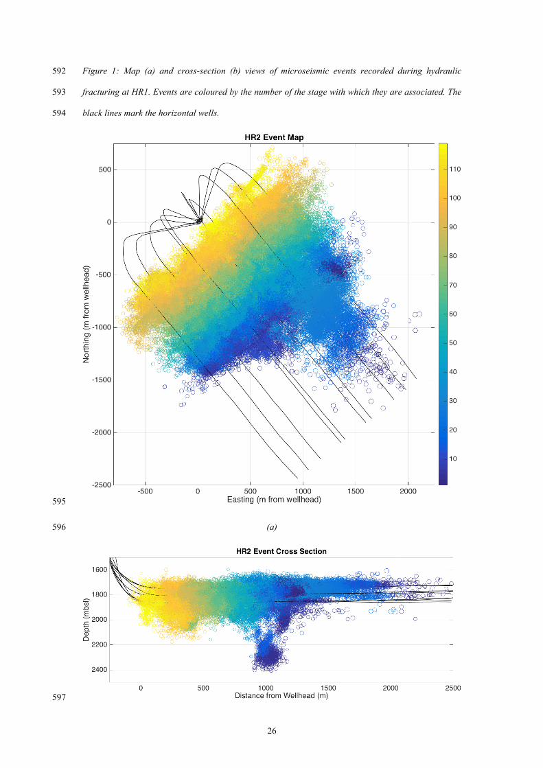
Figure 2: Map (a) and cross-section (b) views of microseismic events recorded during hydraulic 599

fracturing at HR2. Events are coloured by the number of the stage with which they are associated. The 600

black lines mark the tracks of the horizontal wells. 601

602

(a) (b)

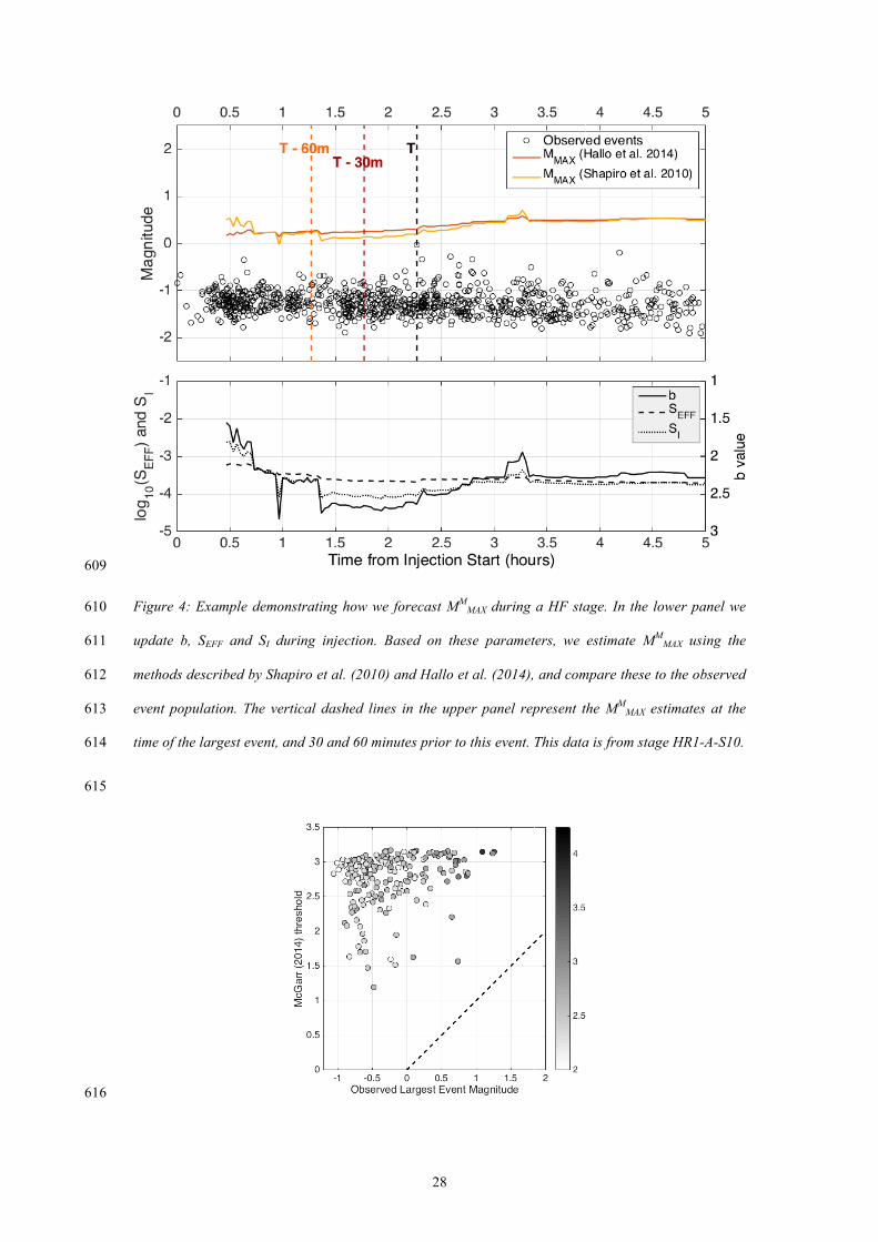
Figure 3: Numerical evaluation of the uncertainties inherent when using equations 6 and 7 to forecast 603

MMAX. A modelled population of events is sampled from a G-R distribution. MMAX is forecast, and 604

compared with the largest event in the simulated population. In (a) we compare the synthetic and 605

forecast values, while in (b) we show a histogram of the differences between the forecast and modelled 606

values. 607

608

28

609

Figure 4: Example demonstrating how we forecast MMMAX during a HF stage. In the lower panel we 610

update b, SEFF and SI during injection. Based on these parameters, we estimate MMMAX using the 611

methods described by Shapiro et al. (2010) and Hallo et al. (2014), and compare these to the observed 612

event population. The vertical dashed lines in the upper panel represent the MMMAX estimates at the 613

time of the largest event, and 30 and 60 minutes prior to this event. This data is from stage HR1-A-S10. 614

615

616

29

Figure 5: Comparison between the observed MOMAX for every stage of both datasets, and that estimated 617

using the McGarr (2014) equation, where MMMAX is directly determined by the injected volume. 618

Symbols are coloured by log10(N), where N is the total number of events per stage. The dashed line 619

indicated a 1:1 ratio. 620

621

622

Figure 6: Comparison between the observed MOMAX for every stage of both datasets, and that estimated 623

using the Hallo et al. (2014) approach. The upper panels show crossplots of observed and modelled 624

MMMAX values, while the lower panels show histograms of MM

MAX - MOMAX. For each case we show the 625

values of MMMAX at the time that the largest event occurred, and at 30 and 60 minutes prior to this time. 626

The symbols are coloured by log10(N), where N is the total number of events per stage. The dashed 627

lines in the upper panels represent MOMAX = MM

MAX. Note that for a handful of stages, robust estimates 628

are only obtained within 30 or 60 minutes of the largest event. In such cases, no MMMAX value is 629

returned at the T – 30 or T – 60 cases, and so there are slightly fewer points plotted for these cases. 630

631

30

632

Figure 7: Comparison between the observed MOMAX for every stage of both datasets, and that estimated 633

using the Shapiro et al. (2010) approach. This figure follows the same format as Figure 6. 634

635

636

(a) (b)

31

(c) (d)

(e) (f)

Figure 8: Testing the ability of the proposed approach to mitigate induced seismicity. In (a) we show 637

MOMAX for each stage that did not reach the MM

MAX > 1 threshold. An example of such a stage, where 638

no mitigation actions would have been taken, is shown in (b). In (c) we show MOMAX for each stage that 639

reached the mitigation threshold, but only after the largest event had occurred. In such cases, any 640

mitigation steps would not affect MOMAX (since the largest event has already occurred). In (d) we show 641

an example of such a stage. In (e) we show MOMAX for each stage that reached the MM

MAX > 1 threshold 642

prior to the occurrence of MOMAX. The triangles show the values of MO

MAX that actually occurred. The 643

squares show the largest event that had occurred prior to reaching the threshold. In (f) we show an 644

example of such a stage. 645

646