Policy Research Working Paper 8360

Gender Differences in Poverty and Household Composition through the Life-cycle

A Global Perspective

Ana Maria Munoz BoudetPaola Buitrago

Benedicte Leroy de la BriereDavid Newhouse

Eliana Rubiano MatulevichKinnon Scott

Pablo Suarez-Becerra

Poverty and Equity Global Practice &Gender Global ThemeMarch 2018

WPS8360P

ublic

Dis

clos

ure

Aut

horiz

edP

ublic

Dis

clos

ure

Aut

horiz

edP

ublic

Dis

clos

ure

Aut

horiz

edP

ublic

Dis

clos

ure

Aut

horiz

ed

Produced by the Research Support Team

Abstract

The Policy Research Working Paper Series disseminates the findings of work in progress to encourage the exchange of ideas about development issues. An objective of the series is to get the findings out quickly, even if the presentations are less than fully polished. The papers carry the names of the authors and should be cited accordingly. The findings, interpretations, and conclusions expressed in this paper are entirely those of the authors. They do not necessarily represent the views of the International Bank for Reconstruction and Development/World Bank and its affiliated organizations, or those of the Executive Directors of the World Bank or the governments they represent.

Policy Research Working Paper 8360

This paper is a product of the Poverty and Equity Global Practice and the Gender Global Theme.. It is part of a larger effort by the World Bank to provide open access to its research and make a contribution to development policy discussions around the world. Policy Research Working Papers are also posted on the Web at http://econ.worldbank.org. The authors may be contacted at amunozboudet@worldbank.org.

This paper uses household surveys from 89 countries to look at gender differences in poverty in the developing world. In the absence of individual-level poverty data, the paper looks at what can we learn in terms of gender differences by looking at the available individual and household level information. The estimates are based on the same surveys and welfare measures as official World Bank poverty esti-mates. The paper focuses on the relationship between age, sex and poverty. And finds that, girls and women of repro-ductive age are more likely to live in poor households (below the international poverty line) than boys and men. It finds that 122 women between the ages of 25 and 34 live in poor households for every 100 men of the same age group. The analysis also examines the household profiles of the

poor, seeking to go beyond headship definitions. Using a demographic household composition shows that nuclear family households of two married adults and children account for 41 percent of poor households, and are the most frequent household where poor women are found. Using an economic household composition classification, households with a male earner, children and a non-income earner spouse are the most frequent among the poor at 36 percent, and the more frequent household where poor women live. For individuals, as well as for households, the presence of children increases the household likelihood to be poor, and this has a specific impact on women, but does not fully explain the observed female poverty penalty.

Gender Differences in Poverty and Household Composition through the Life‐cycle: A Global Perspective1 

Ana Maria Munoz Boudet, Paola Buitrago, Benedicte Leroy de la Briere, David Newhouse, Eliana Rubiano Matulevich, Kinnon Scott, Pablo Suarez‐Becerra with the Global Solution Group on Welfare Measurement and Capacity Building. 

JEL codes: I3, J1, O1 

Key words: Poverty, Gender, Lifecycle, Women, Household 

1  Ana Maria Munoz  Boudet  is  a  Senior  Social  Scientist with  the  Poverty  and  Equity Global  Practice  at  the World  Bank, David Newhouse and Kinnon Scott are Senior Economists with  the same group. Benedicte de  la Briere  is a Lead Economist with  the Gender Global Theme Department at  the World Bank, Eliana Rubiano Matulevich  is  an Economist with  the  same  team. Paola Buitrago  and  Pablo  Suarez‐Becerra  are  both  Economist  Consultants  with  the  World  Bank.  The  authors  can  be  contacted  at amunozboudet@worldbank.org. The World Bank’s Global Solution Group on Welfare Measurement and Capacity Building is a team of statisticians and economists responsible for producing the global monitoring data base (GMD)used for this study.  This paper was commissioned as a background paper  for UN Women’s  flagship reports “Turning promises  into action: Gender equality  in  the  2030  Agenda  for  Sustainable  Development”  and  the  upcoming  Progress  of  the World’s Women.  Funding was provided by UN Women. The team would like to thank Ginette Azcona, Shahra Razavi, and Papa Seck from UN Women for their comments and feedback. The team also benefited from comments by Caren Grown, Carolina Sanchez‐Paramo and Carlos Silva from the World Bank. 

2 

Introduction  

Eradicating poverty in all its forms and dimensions, including extreme poverty, is among the main challenges  the  global  community  and  governments  face.  Achieving  this  goal  by  20302  will  require  for governments to implement a set of policies aimed at investing in human capital, improving labor markets, expanding  social  protection,  and  implementing  targeted  policies  to  help  groups  of  the  population experiencing specific disadvantages. Various population subgroups, be  they based on gender, ethnicity, race, or income, have faced and continue to face barriers that have slowed the rate of poverty reduction. Understanding how poverty affects subgroups in different ways is critical to realizing welfare goals.  

A key area of concern has been the extent to which women and men face different levels of poverty and distinct  barriers  to  poverty  reduction. Our understanding of  these differences,  however,  has been constrained by the available data. In the standard approach to measuring poverty, the primary source of information is household surveys and the key indicator  is a money‐metric measure of welfare based on consumption or income. Data are collected on the consumption or the income of each household, and not always of each  individual  living  in  those households3.  This masks variation  in  individual‐specific welfare levels, as intra‐household disparities in access to income, consumption and other entitlements cannot be measured. The result is that gender differences in poverty rates are muted or not at all visible.4  

In this study we show that, even with the existing constraints (which we discuss in greater detail below), there is still much to be learned about poverty and gender. Taking advantage of a global database of harmonized country‐representative surveys constructed by the World Bank, we look at the ways in which men and women experience poverty differently. The focus of the study is on four key questions. First, in the absence of individual‐level poverty data, what can we learn in terms of gender differences by looking at individual‐level information? Here, we focus on the relationship between sex and poverty and explore available data to us such as age, location, education, marital status, and labor market participation. This is done  at  global  level  but  is  also  explored  at  the  regional  level.  Second,  to  the  extent  that  there  are differences by sex, are these related to specific moments of the lifecycle of women and men? Third, at the household level, are there specific types of households that are more likely to be poor than others and how does gender factor  into this? And, finally, what are the channels that  link individuals and households to poverty?  

To answer these questions, we use two approaches. First, the study provides gender profiles of the poor at the global level, taking into account sex, age, marital status, education and employment. The global profiles  are  supplemented  with  regional  profiles  to  begin  to  understand  how  geography,  gender  and poverty are related. Second, the study looks at household profiles of the poor. Given the limitations of work looking at households only by the sex of the household head, this study proposes two new typologies of households, a demographic one and an economic one.  

This study makes three key contributions to the literature on poverty and gender. First, it provides a global picture of the connections between gender and poverty. By using the same global database and the same measure of poverty used by the World Bank to monitor the first Sustainable Development Goal and its own goal of eradicating extreme poverty, we are able to provide a global picture of poverty and 

2 SDG Goal 1: By 2030, eradicate extreme poverty for all people everywhere, currently measured as people living on less than $1.25 a day. (Resolution adopted by the UN General Assembly on 25 September 2015. 70/1).  3 In addition, the data is generally collected from one or two respondents “best informed”, which may lead to under‐estimates of consumption/income  if not all  consumption/income  is shared and visible, which  is  the case when  individuals work  in different workplaces and keep separate accounts. 

4 Grown, 2014; Lanjouw, 2012; Deere et al., 2012. 

3 

 

gender as well as regional comparisons. Second, by expanding on household typologies beyond headship, we show that using information on the full composition of the household, not just the sex of the head of household,  contributes  to  a  better  understanding  of  gender  differences  in  poverty.  Finally,  the  study introduces a lifecycle approach that sheds new light on how poverty affects people over time. 

The present study provides a compelling story of how a lifecycle approach, including age, family formation and living arrangements play a crucial role in the way women and men experience poverty. The analysis is presented in the following manner. Section 2 contains a brief literature review related to the key issues of the poverty and gender intersection as well as a description of the data set used for the analysis. The third section looks at gender profiles of the poor in both demographic and economic terms and some of the drivers of the observed differences. The work presented in Section 4 addresses the limitations of standard head of household analysis by introducing two new typologies of households and exploring how gender, poverty and household type are connected. The section ends with a discussion of the channels that link household type and poverty.  

What do we know about gender and poverty? 

 Measuring poverty is a complex task 

Measuring global poverty is a complex, data‐intensive exercise. Data used comes from nationally‐representative household surveys that capture a money‐metric measure of welfare – either consumption or  income. Each data set  is harmonized and then a welfare aggregate  is constructed. The World Bank’s database includes almost 150 surveys from developing countries, of which 104 fall in the time period of analysis used in this report. This collection of survey data is then combined with complementary data on population  size  (growth),  inflation,  real  economic growth, and Purchasing Power Parity  (PPP) exchange rates to produce country‐level,  regional and, global estimates of poverty.5 From there, population‐level poverty figures are estimated by taking the household level welfare measure and dividing it by the number of people in the household. This assigns all consumption evenly to household members. Those individuals whose per capita consumption is below the value of the  international poverty  line (US1.90 in 2011 PPP terms) are classified as living in extreme poverty.6  

The fundamental concern with this measure of poverty is that it assumes consumption or income is  distributed  and  shared  evenly  within  a  household.  True  individual  welfare  is  not  observed  and  the household  measure  often  ignores  intra‐household  disparities  in  access,  consumption,  and  other entitlements  (Grown,  2014;  Lanjouw,  2012;  Deere  et  al.,  2012),  making  the  uniform  distribution  of consumption (income) to all household members inadequate. A substantial body of literature suggests that not all members of the household share equally the resources of the household (see, for instance: Haddad and Kanbur, 1990; and Chant, 2010).  In fact, household  income (consumption) may bear no relation to women’s poverty because women may not necessarily be able to access it (Bradshaw 2002; Chant 2006, 2010; Bessell 2010, 2014). Predictions derived from a unitary model of household behavior, based on the notion of a single benevolent decision‐maker or consensus amongst members, often do not find empirical support (Lundberg et al., 1997). In summary, the small differences in observed poverty between men and 

                                                            

5 See Castañeda et al., 2016 for more detail. Note that national poverty measures differ as both the welfare aggregate and the value of the national poverty line will vary from the harmonized variables and international poverty line used here (World Bank, 2015).  6 The international poverty  line corresponds to the mean of the poverty  lines found in the poorest 15 countries ranked by per capita consumption (World Bank, 2015). 

 

4 

 

women may be less a reflection of reality and more a result of the fact that poverty is measured at the household level and by assumption all household members are classified as either in or out of poverty, and, the  ratio, when  considering  all  ages,  of males  to  females  is  roughly  50/50  in  both  poor  and  non‐poor households.7 

In  an  attempt  to  get  around  this  fundamental  limitation,  various  researchers  have  developed alternative methods.  The most  common  is  to  classify  households  according  to  headship  and  compare poverty across female‐ and male‐headed households. However, several studies have contested the use of headship as a relevant analytical category for a number or reasons. First, countries use different and often non‐comparable definitions of the terms “household” and “head of household”. Second, there is ambiguity in the term “head of household” when the assignment of headship is left to the judgement of household members (or the survey enumerator). Third, the term “head of household” is not neutral; it is loaded with additional meanings that do not reflect internal conflicts in the allocation of resources (Buvinic and Gupta, 1997;  Quisumbing  et  al.,  2001;  Budlender,  2008).  In  addition,  the  link  between  female  headship  and poverty may not be straightforward partly because female‐headed households are a highly heterogeneous group and may well reflect self‐selection, demographic processes, or others8. Aside from socio‐economic status,  female  (and  male)‐headed  households  show  significant  variation  in  terms  of  age,  relative dependence, household composition, lifecycle, and access to resources beyond the household unit, among others, making such classification not very useful.  

The fact that differences in poverty rates between female‐ and male‐headed households cannot necessarily  be  ascribed  to  gendered  differences  in  earnings,  access  to  employment  or  control  over resources, has  led authors to explore alternative classifications of headship. Rogan (2013) explores four alternative classifications of households based on the absence of male householders or the dependence on  female  income  in  post‐apartheid  South  Africa.  The  findings  of  this  study  suggest  that  there  is  an association between self‐reported female headship and a female household member being identified as the main breadwinner. However, under a different classification of household head (e.g. who is the main responsible individual for the household that can be identified in the data), then the finding that female‐headed households are increasingly more vulnerable to poverty (relative to male‐headed households), is even stronger. A recent report also reveals that working‐age women are more likely than men to be poor when they have dependent children and no partner to contribute to the household income. At older ages, women in developed countries are more likely than men to be poor, particularly when living in one‐person households (United Nations, 2015). 

In  addition  to  looking  at  headship,  there  are  several  other  approaches  to  circumventing  the limitations of the household poverty measure. There are some innovative attempts to extract individual‐level welfare information from household surveys. Such studies attempt to draw inferences about intra‐household resource allocation by, for example, estimating the fraction of household expenditure that  is consumed by each family member.9 Dunbar et al (2013) estimate individual resource shares for adults and children in Malawi by observing how expenditures on a single private good that can be ascribed to individual household members  vary with  income  and  household  size.  Their  results  indicate  that  the  incidence of poverty is significantly higher for women (85 percent) than men (60 percent) and even higher for children (95  percent).  Using  a  unique  survey  for  Senegal  that  collected  consumption  data  for  sub‐groups  of household members (“cells”) in non‐nuclear households, Lambert et al. (2014) and De Very and Lambert 

                                                            

7 Castañeda et al. (2016) 8 There are multiple explanations for why women head households and these differences can lead to different outcomes that are not necessarily negative for women’s well‐being (Chant, 2003, 2008).  9 Dunbar et al. 2013; Bargain et al. 2014. 

5 

 

(2017) find significant inequalities within the household and a sizeable gender gap in consumption. Cells headed by males have approximately 77 percent higher consumption levels than cells headed by females. This difference is largely driven by inequality in non‐food consumption. In Senegal, De Vreyer and Lambert (2017) collect consumption section for small groups of individuals within each household, and use that data to create an individual measure of consumption, leading to findings of within household inequality, and evidence of poor individuals living in non‐poor households. Brown, Ravallion and van de Walle (2017) use nutritional  status  as  a  proxy  for  individual  poverty  and  find  evidence  of  undernourished  women  and children living in households that are above the bottom 40 percent of the poverty distribution (measured in  terms of assets).  Studies by Haddad and Kanbur  (1990) and Bargain et al  (2014) also  find significant differences by sex when intra‐household analysis  is done. While these findings are important,  individual allocations within households are rarely observed. There is no standard process to establish equivalence scales,  which  means  relying  on  strong  assumptions  to  understand  the  sharing  process  (Klasen,  2004; Grown,  2014)10.  A  further method  for  assessing  intra‐household  welfare  uses  data  on  individual  asset ownership for housing,  land and business assets. Deere et al. (2012) show that the distribution of asset ownership  by  sex within  households  is much more  equitable  in  some  Latin American  countries  than  a headship analysis would suggest. It might be the case that women in male‐headed households often own property, either in their own right or as joint property with their spouses. Brown, Ravallion and van de Walle (2017) use asset wealth in households as a proxy for household poverty, and nutritional status to measure individual  deprivation  of  women  and  children.  They  find  evidence  of  deprived  women  in  non‐poor households measured by assets holdings. Still, the number of surveys which provide data that can be used for individual measures of poverty is quite limited and thus this approach can only be used in a handful of cases.  

Although exploratory work is also ongoing to determine feasible means to measure individual‐level welfare in the context of nationally‐representative surveys, individual‐level welfare data is not yet available for  a  representative  number  of  countries.  Multidimensional  approaches  to  poverty  complementing standard  measures  with  non‐monetary  metrics  have  become  firmly  established  as  a  complement  to income‐based approaches. Alkire and Foster (2011) suggest a counting approach based on the concept of capabilities, which allow for both identifying the poor and aggregating the poverty measure. The most well‐known  measure  is  the  Multidimensional  Poverty  Index  (MPI)  proposed  by  Alkire  and  Santos  (2014), including  three equally weighted poverty dimensions—health, education and  living standards—that are captured  by  a  number  of  indicators.  Several  studies  have  estimated multidimensional  poverty  among women  using  the  multidimensional  approach  and  comparisons  with  standard  poverty  measures  (e.g. income and asset poverty)  show  that  considering additional dimensions  leads  to  substantially different results (Batana, 2013). However, these measures, with few exceptions, have focused on a household‐level assessment of poverty  and hence,  just  like monetary approaches cannot provide  information on  intra‐household dynamics (Gaddis, 2016). Furthermore, measuring multidimensional poverty at the individual level  requires multiple  decisions  regarding  dimensions,  indicators,  weights  and  cut‐offs,  among  others (Ravallion, 2011).  

In summary, the present model of welfare measurement may hide differences in poverty by sex by not providing individual‐level information. While the ability to disaggregate or assign household spending or income to individuals is limited, the present paper explores how existing data, globally representative and harmonized at the global level, can shed light on gender differences by looking across the lifecycle and 

                                                            

10 The limited agreement on how to estimate equivalence scales (Deaton and Paxon 1996, Deaton 1997) results  in a variety of equivalence scales  that are not standard and  lead to different results across countries, as poverty metrics are sensitive  to  the equivalence scale used. Varying the economy of scale parameter may change the relative poverty risks of different demographic subgroups of the population, notably the elderly and children (Lanjouw et al. 2000). 

6 

 

how other indicators of welfare can provide important insights into the way men and women experience poverty.  

How women and men experience poverty has multiple dimensions 

Understanding how different individuals experience poverty is crucial for the design of policies to reduce poverty. Gender differences are among the most important. Gender inequalities make women and girls more vulnerable  than men and boys  to poverty  (World Bank, 2011) and they affect how men and women react to changes in poverty status. Differences in gender norms, intra‐household division of assets, work and responsibility and relations of power drive these disparities (Grown, 2014). In many countries, females  have  lower  levels  of  education,  lower  ownership  and  control  over  assets,  and  lower  social indicators than men. Bargaining power is affected by control of resources (e.g. assets and income), legal rights, skills and knowledge, the capacity to acquire information, education, etc. Social norms also set the context  of  intra‐household  negotiation  over  time  allocations,  resources,  and  access  to  labor  markets (Quisumbing, 2010). Social policies that facilitate universal access to services and mitigate shocks can serve to  level  the playing  field and change both  social norms and bargaining power. A  few examples  include policies  providing  adequate  water  and  sanitation  in  schools,  as  in  Almeida  and  Oosterbeek,  2016, conditional  cash  transfer  programs  where  the  benefits  are  given  to  women  such  as  the Progresa/Oportunidades program in Mexico, or unemployment insurance and social pensions.  

Access  to and control over  income and assets  is an  important component of welfare especially when a household dissolves, whether due to separation, divorce or death. This frequently determines the livelihoods  available  to members of  household,  and  influences  the distribution of  resources within  the household (Deere et al. 2012). Furthermore, it underpins women’s greater vulnerability to poverty. Agbodji et  al.  (2013)  show  that  inequalities  in education and employment  largely explain gender differences  in poverty in Burkina Faso, while differences in access to assets and credit are the main sources of gender differences in Togo.  

Gender inequalities in labor markets also contribute to women’s greater vulnerability to poverty. Evidence suggests that even after controlling for individual characteristics, women in Latin America have a lower probability of participating in the labor market, a lower probability of being formal workers, and lower hourly wage remuneration (Costa et al., 2009). Moreover, because women are more likely to be informally employed,  they are also more prone  to be excluded  from non‐wage benefits  such as health  insurance, pensions, paid sick leave and maternity leave (ILO 2016). Women are more likely to be providers of unpaid care within the household (for children, those with disabilities and the elderly) (as shown in World Bank 2012). Tax policies also affect women and men differently over the lifecycle, and may not take into account transitions in roles and household types. For instance, the presence of children in combination with the tax treatment of the household’s second earner in systems that tax the household’s joint income, may lead to further fall in women’s labor force participation (Grown and Valodia, eds. 2010).  

Since specialization in any activity typically requires costly and considerable investments, gender differentials  in early  investments can result  in  larger gender differentials  later  in  life. Lokshin and Mroz (2003)  examine how a  spectrum of  gender  differences  vary  across  income groups  over  the  lifecycle  in Bosnia  and  Herzegovina.  The  results  suggest  that  the  main  source  of  gender  inequality  comes  from different investments in girls’ and boys’ education that increase with declines in income levels. At the same time, single women that come from poor households could be at a great risk of poverty because of limited labor market opportunities available to them compared than those available for males (Rosenzweig and Wolpin, 1994). 

7 

 

As it can be seen, much of the literature on gender differences and poverty are based on specific countries or case studies, and global or regional studies are infrequent11. The goal of the present paper is to expand this discussion to the bulk of the developing world and have a more global picture of poverty and gender. At  the same time, the study makes regional comparisons that shed further  light on critical policy concerns. 

Data sources 

This study uses the Global Monitoring Database (GMD), which is a collection of globally harmonized household  survey  data  developed  by  the World  Bank’s  Poverty  and  Equity  Global  Practice.  The  GMD contains  a  combined  sample  of  104  household  surveys  containing  records  representing  6.8  million individuals from 89 developing countries. Full details on the background of the GMD are given in Castañeda et al (2018). A crucial feature of the GMD is that, in general, the welfare aggregates are the same as those used  to  compute  the  poverty  estimates  that  the  World  Bank  publishes  via  PovcalNet  and  the World Development  Indicators.12,13 These aggregates are based on a money‐metric measure of welfare, either household per capita consumption or income, depending on the concept used to measure national poverty in each country. The analysis in this paper uses those surveys in the GMD collected in 2009 or later in an attempt to balance the competing goals of increasing global coverage while minimizing error that arises from extrapolating poverty figures forward to 2013.14  

The present version of the GMD is missing several labor variables in Sub‐Saharan Africa. To rectify this,  a  process  is  underway  to  integrate  an  additional  data  set  (the  International  Income  Distribution Dataset) into the GMD. For this study, additional information on labor and education outcomes was merged from this additional dataset for 17 sub‐Saharan African countries.15  

It is important to note that regardless of the source, in several cases the labor information available is of insufficient quality to include the survey in the analysis. As economic empowerment is a key feature of household composition, particularly when the economic typologies of households is applied (see Section 4 below),  surveys were discarded  if  reported  labor market outcomes appeared  inconsistent with other sources of data for the country.16 For the 89 countries covered in the GMD a total of 18 were dropped due 

                                                            

11 One of the few examples of regional work include ECLAC (2016) report including the poverty femininity index for Latin America and the Caribbean.  

12 Important exceptions are India and China. In China, the analysis is based on the China Household Income Project Data from 2013, which is publicly available. However, the poverty line has been determined such that the poverty rate matches the official World Bank estimates (See Castaneda et al, 2018). For India, the data in this study is taken from schedule 10 of the Indian National Sample Survey,  because  it  contains  information  on  labor  market  outcomes.  As  in  China  the  poverty  line  is  set  at  the  percentile corresponding to the official World Bank estimates, which in India are derived from schedule 1 of the National Sample Survey.  13 The term welfare refers to either income or consumption per capita, depending on which measure is used by the country for their national estimates. For more information on how these welfare aggregates are constructed, see Ferreira et al (2015). 14 As the GMD is updated when new surveys become available and are harmonized, it is important to note the ‘vintage’ of the data set used. Specific results of this analysis could vary as new data sets are added to the GMD although it is not expected that the overall story would be affected. The poverty and gender analysis presented here is derived from the September 2016 version of GMD with estimates of poverty figures lined up to (extrapolated to 2013). 15 The countries are: Burkina Faso, Chad, Republic of Congo, Democratic Republic of Congo, Ethiopia, Guinea, Malawi, Mauritius, Niger, Nigeria, Rwanda, Senegal, Sierra Leon, South Africa, Sudan, Tanzania, and Uganda. The I2D2 data set has been used for previous work on gender and labor at the WB.  16 Surveys for five countries were discarded because information on each individual’s primary activity was either not present in the data or missing for more than 30 percent of the observations. Surveys from an additional two countries were discarded because, for more than ten percent of individuals, information on employment status was present even though the person’s primary activity 

 

8 

 

to  quality  concerns  for  some  of  the  analysis  in  this  study  (particularly  the  analysis  involving  economic participation variables). This reduced the sample to 71 countries. for any analysis including labor‐related variables. For all other analysis the full 89 countries sample is used17.  

Figure 1 shows the final sample. Tables 1 and 2 in the appendix show the nature of the sample and the  sample’s  coverage  in  number  of  countries  and  population  based  on  figures  from  the  UNDESA Population Division.  Countries  in  the  sample  have  a  total  population  of  4.8  billion  persons,  roughly  75 percent of the developing world population of 6.5 billion. Nearly 78 percent of the sample originates  in middle‐income countries, and East and South Asia account for nearly two thirds of the sample. The GMD sample has high regional coverage of developing countries in South Asia, East Asia and the Pacific, Latin America and the Caribbean, and Europe and Central Asia (above 87 percent); and partial coverage of Sub‐Saharan Africa (74 percent). Because of low coverage in Middle East and North Africa (4.1 percent), results from this region are not presented18. 

 Figure 1: Coverage of Data of the GMD database 

  

Depending on how each country measures poverty, welfare aggregates are based on household per  capita  consumption  or  income.  For  all  of  them,  poverty  is  defined  based  on  whether  per  capita household welfare, converted to international dollars using 2011 PPP conversion factors, falls below the poverty line. The World Bank uses the international poverty line (IPL_ of $1.90 per person per day, which corresponds  to  the mean  of  the poverty  lines  found  in  the poorest  15  countries  ranked by  per  capita consumption, to define extreme poverty. For the remaining of the paper, references to poor individuals of 

                                                            

was coded as ‘not working’ suggesting miscoding in these surveys. Six other countries had to be dropped since, in their surveys, either the share of adults out of the labor force was less than 10 percent or all adults were reported as being out of the labor force. These surveys may have used non‐standard recall periods for the labor statistics. Finally, due to a miscoding of employment status that made it impossible to distinguish between unpaid, paid, and self‐employed workers in the survey data, another five countries had to be dropped from the analysis. 17 The sample used is noted for each table and figure in the paper. 18  Regional  aggregates  follow  the World  Bank  geographic  regions  classification  (see  http://www.worldbank.org/en/where‐we‐work). 

9 

 

households will be with regards to the IPL (extreme poverty). As will be discussed in more detail in Section 2 below, all persons in poor households are considered to be poor and all persons in non‐poor households are considered to be to be non‐poor. This assumes that all household members enjoy the same standard of living, which, as discussed below, may understate the gender dimensions of poverty.  

Gender Profiles of the Poor  

Globally, the number of people  living on less than $1.90 a day (below the International Poverty Line)  is  654.9 million, which  corresponds  to 12.5 percent  of  the  total  population  included  in our GMD sample. Table 1 shows that nearly half of the poor live in Sub‐Saharan Africa (51.3 percent or 302.7 million), followed closely by South Asia (251.6 million). Slightly more than half of the poor are women (330 million), and men account for 49.7 percent of the poor (325 million). Poverty rates for females and males are similar (12.8  and 12.3 percent,  respectively).  These  rates  vary  across  regions,  but  gender differences  are only statistically  significant  in  South  Asia,  where  female  poverty  rates  are  15.9  percent,  compared  to  14.7 percent for males. Worldwide, this translates to 104 women living in poor households for every 100 men. In South Asia, 109 women live in poor households for every 100 men19.  

 Household‐level information can provide relevant insights when it comes to the gender profiles of the poor. Although, in the aggregate, female and male poverty rates are very similar, as shown in the tables below20, they mask variations according to individual characteristics, which are helpful to start developing a more  disaggregated  understanding  of  potential  differences  between men  and women  in  relation  to poverty.  

 Table 1. Proportion (and number) of poor population, poverty rates, and distribution of the poor by sex and region. 

1.a. Population living in poverty by sex 

   Number of poor (millions) 

% poor of population 

Female poverty  rate 

Male poverty rate 

Female share of poor 

Male share of poor 

East Asia and Pacific  67.6  3.6  3.6  3.6  48.8  51.2 

Europe and Central Asia  3.3  0.8  0.8  0.8  51.6  48.4 

Latin America and Caribbean  29.4  5.3  5.5  5.2  51.8  48.2 

Middle East and North Africa  0.3  1.9  2.0  1.9  50.7  49.3 

South Asia  251.6  15.3  15.9  14.7  50.7  49.3 

Sub‐Saharan Africa  302.7  43.2  43.4  42.9  50.2  49.8 

Total  654.9  12.5  12.8  12.3   50.3   49.7 

    

                                                            

19 These numbers refer to the weighted population ratio in the GMD dataset. As a reference, the population ratio (males per 100 females)  was  estimated  at  101.5  for  2015,  variating  from  103.6  for  lower‐middle  income  countries,  to  98.8  for  low‐income countries. The ratio for South Asia was estimated at 106.2 (Source: United Nations, Department of Economic and Social Affairs, Population Division (2017). World Population Prospects: The 2017 Revision, custom data acquired via website) 20 As noted earlier, the analysis assumes that all persons living in poor households are poor and all persons in non‐poor households are non‐poor.  Therefore,  female  and male poverty  rates  are defined  as  the percentage of women and men who  live  in  poor households. 

10 

 

1.b. Regional distribution of the poor by sex 

   Female  Male   Total 

East Asia and Pacific  10.0  10.6  10.3 

Europe and Central Asia  0.5  0.5  0.5 

Latin America and Caribbean  4.6  4.3  4.5 

South Asia  38.7  38.2  38.4 

Sub‐Saharan Africa  46.1  46.3  46.2 

Total  100  100  100 

Note: Total sample 89 countries Source: WB Staff’s calculations based on GMD. 

 The small differences we observe in the general numbers (disaggregated by sex alone) reflect the 

facts that: (i) poverty is measured at the household level and by assumption all household members are classified as either in or out of poverty, and (ii) the ratio of males to females is roughly 50/50 in both poor and non‐poor households, (iii) 50 percent of the poor are children, with no observed gender differences in the poverty headcount rate21. Measuring poverty at the household level assumes no intra‐household inequalities in access to income, consumption and other entitlements. Hence, gender differences in poverty rates are muted when looked through the lens of household‐level poverty.  

Where are the gender differences? Demographic characteristics 

Differences in poverty rates between women and men become more salient as we start looking at different  population  subgroups  by  available  demographic  and  other  characteristics.  For  example,  take residence. Globally, we can observe that the majority of the poor live in rural areas, and 18.2 percent of rural residents live on less than $1.90 a day. The corresponding rate for urban residents is 5.5 percent. This geographic difference in poverty rates, combined with the concentration of the poor in rural areas, means that about 80 percent of the poor live in rural areas, compared with 55 percent of the total population. Female poverty rates are slightly higher than male poverty rates in both urban (5.7 for women and 5.4 for men) and rural areas (18.7 for women and 17.9 percent for men).  Women represent a larger share of the poor in urban areas, and men represent a larger share of the poor in rural areas (Figure 2b). However, these differences are not statistically significant at the global  level.  In all  regions, poverty rates are higher for women than for men. Gender differences, however, are again only significant in South Asia where female poverty rates are about 1 percentage point higher in both urban and rural areas.  

We also know that the poor tend to be young, and children are particularly at risk for poverty in the sample of 89 countries. Over one in five girls and boys ages 0‐14 live in a poor household and they represent 44 percent of the poor population. As already documented by Newhouse et al (2017) using the same dataset, 19.5 percent of all children younger than 18 are estimated to live on less than $1.90 per day, a bit over double the estimate for adults (9.2 percent). Girls and boys are consistently poorer than adults and seniors, and poverty  is higher for children younger than 5 years of age, regardless of sex22. Among females, girls under 15 are the poorest. Their poverty rate  is 8.5 percentage points higher than that of young women age 15‐24, and over 14 percentage points higher than that of senior women (only 6.7 percent 

                                                            

21 See Newhouse et al (2016) and Castañeda et al (2018) 22 In this paper/section, children are individuals aged 0‐14, young adults are 15‐24, adults are defined as individuals ages 18‐59, seniors are 60 and above. Prime‐working age individuals are 25‐54 and mature individuals are between 55 and 60 years of age.  

11 

 

of senior women are poor). The same pattern holds for males. Boys under the age of 15 are the poorest and their poverty  rate  is 8.4 percentage points higher than that of young men ages 15‐24 and over 12 percentage points higher than that of senior men (only 7.3 percent of senior men are poor).  

 

Figure 2. Poverty rates and geographic distribution of the poor by sex 

2.a. Poverty rate geographic area and sex  2.b. Geographic distribution of the poor by sex 

 

Note: Total sample 89 countries Source: WB Staff’s calculations based on GMD. 

 

Children are the poorest across all regions, but the patterns vary by region (Appendix Figure A1). For example, in Sub‐Saharan Africa, 49.3 percent of girls and 49.5 percent of boys live in poor households and boys represent a slightly larger share (51 percent) of poor children than girls do. Differences with other age groups are even starker than the global ones: boys and girls under 15 years of age are 10 percentage points poorer than their young adult (15‐24) counterparts, and girls are 17.2 percentage points poorer than females above 60. In contrast, in South Asia, girls are poorer than boys (22.2 and 20.1 percent, respectively) and more numerous than boys among the poor (50.5 percent), but differences in poverty rates between children and older adults —although sizable—are smaller than in other regions.  

 

   

5.7

18.7

5.4

17.9

0

5

10

15

20

Urban Rural Urban Rural

Female Male

Percentage

79.8 80.2

20.2 19.8

0

20

40

60

80

100

Female MalePercentage

Rural Urban

12 

 

Figure 3. Female and male poverty rates by age group 

 Note: Total sample 89 countries Source: WB Staff’s calculations based on GMD. 

 

More  importantly,  introducing  age  as  an  element  when  measuring  poverty  starts  to  reveal important gender differences. Poverty decreases with age, especially between childhood and adulthood but it decreases at different ages for women and men. Poverty rates decrease sharply for women and men as they reach adulthood and tend to stabilize after 50 years of age. By age 25 (and up to age 34), women are two percentage points poorer than men, a significant and sizeable difference. In this age group, there are, on average, 120 women living in poor households for every 100 men. This gap coincides with the peak productive and reproductive ages of men and women, and can be related to factors such as household formation and income generation for both men and women, and the  implications of such processes on their welfare. For example, it has been well documented that women’s labor force participation goes down during their reproductive years, particularly when they have young children (see among others Aguero and Marks 2008, Goldin and Katz 2002). This pattern  is consistent across regions, but gender differences  in poverty rates vary widely. For the 20‐34 age group, the average gender poverty gap ranges between 0.12 percentage points in Europe and Central Asia to 7.1 percentage points in Sub‐Saharan Africa (see annex for graphs per region).  

If we are able to see differences at the regional  level, does the variation  increase further when looking within the regions to the country‐level differences? Not much. As in the larger groupings, female and male poverty rates are similar in most countries for which we have data available. Figure 4a shows that gender differences  in poverty  rates are  rather  small when all  ages are averaged and poverty  rates  are disaggregated  only  by  the  sex  of  household members. More  interestingly,  consistent with  overall  and regional patterns, gender differences in poverty rates at the country level are more evident when focusing on individuals aged 25‐34 (Figure 4b). Women in this age group are at least one percentage point poorer than men in 65 of the 89 countries included in the GMD sample.  

The gap in poverty rates between men and women aged 25‐34 is wider in the poorest countries. Female poverty rates are between 5 and 20 percentage points higher than male poverty rates in 17 of the countries  included  in  the  database.  These  are  also  the  countries  with  overall  poverty  rates  above  35 percent. Except for Haiti, all these countries are in Sub‐Saharan Africa.  

 

 

0

5

10

15

20

25

0‐4 5‐9 10‐14 15‐19 20‐24 25‐29 30‐34 35‐39 40‐44 45‐49 50‐54 55‐59 60‐64 65‐69 70‐74

Women Men

13 

 

Figure 4. Gender differences in poverty rates 

4.a. Poverty rates difference (male‐female). All ages  4.b. Poverty rates difference (male‐female). 25‐34 age group 

   

  

Notes: The dark lines indicate a total poverty rate higher than 35 percent. Total sample 89 countries Source: WB Staff’s calculations based on GMD.  

 

In  later  life, gender differences  in global poverty rates tend to disappear and the percentage of poor women is slightly lower than that of men. Again, the global numbers mask regional differences, partly because of the population composition in each region, and life‐expectancy differences by sex. For example, the difference  in poverty  rates between women and men age 60 and above  is  small across all  regions, except for Sub‐Saharan Africa, where men are 8 percentage points poorer than their female counterparts and where they represent a larger share of the poor than women. However, in this region, this age group accounts for about five percent of the population and four percent of the poor population, with no gender differences in either population shares.  

What else do we know of men and women in the age group where the greater differences can be observed? We know that about 68 percent of women and men age 18 or above are married, and that by age 70 percent of the poor of that same age are married23. For those of a younger age, we find that ten percent of poor girls are married, compared with five percent of poor boys. For both, these rates are higher than those in the total population (six and two percent respectively). Figure 5 summarizes marital status for the poor. On average, we see small and not significant differences in poverty rates between women and men when looking at marriage and cohabitation. Differences arise when looking at those who have 

                                                            

23 Globally, the average mean age of marriage is of 26 years of age (source World Bank Genderstats) 

20 15 10 5 0 5

Male poverty is higher

Female poverty is higher

20 15 10 5 0 5

Male poverty is higher

Female poverty is higher

Total poverty >35 

14 

 

never married (men more frequently than women, of which one third are living in India), those who are divorced or separated (women representing the majority of the poor in that group, a quarter of them being in Latin America and the Caribbean), and those who are widowed (women more frequently than men).  

 Figure 5. Distribution of the poor by sex and marital status (ages 15+) 

 

Note: Total sample 89 countries Source: WB Staff’s calculations based on GMD. 

 

A  focus  on  gender  differences  in  poverty  through  the  lifecycle,  as  captured  by  age  transitions (childhood  to  adolescence,  to  adulthood,  to  elder  years)  and  the  related  changes  in  own  household formation (marital status and living arrangements, and presence of children), reveals meaningful gender differences in poverty rates.  

Early marriage is correlated with higher poverty for girls and boys, and marital shocks at that age make girls extremely vulnerable to poverty. Girls who are married or widowed in the 15‐17 age group (only one percent of all poor girls) are 11.2 and 30.6 percentage points more likely to live in poor households compared to the average young women of that same age, among whom the most frequent marital status is single or never married24. Married young males have poverty rates 17 percentage points higher than the average men of that same age group. But, contrary to what we observe with girls, poverty rates are lower for the less than one percent of boys (0.13 percent) who report being divorced or widowers.  

Figure 6 shows the impact of changes in marital status on other age groups, and how certain life‐events at specific age groups correlate with higher poverty rates. Marriage is the most common marital status for women and men aged 18‐64 (as noted by the size of the marker), and for both men and women, widowhood  when  experienced  in  that  age  group  shows  higher  poverty  rates.  For  women,  divorce  or separation also  increases  their poverty  level  (marginally) when compared with  those who are married, whereas  poverty  rates  are  lower  for  men  who  are  divorced  or  separated  than  for  their  married counterparts. Divorce  and  separation  affect women more negatively  than men,  but do not  necessarily translate into higher poverty rates for women. Yet, divorced/separated women aged 18‐49 are more than 

                                                            

24 Marital status is only available for individuals 15 years old and above in the GMD. The data refers to marital status at the time of the survey. 

66.8 65.7

2.7 2.4

16.928.5

3.31.0

10.22.3

0

10

20

30

40

50

60

70

80

90

100

Women Men

Percent of poor

Married Living together Never married Divorced/ separated Widowed

15 

 

twice as likely to be poor than divorced men in that same age group. For women, widowhood, at all ages is a poverty  increasing factor, although of declining value as women age. For men and women, remaining single by age 50‐64 puts them at a higher poverty rate than their married peers of the same age. 

 Figure 6. Female and male poverty rate by age group and marital status 

6.a. Female poverty rate 

  

6.b. Male poverty rate 

 Notes: The size of the dot represents the relative weight of each group within the total poor for the age group. Total sample 89 countries Source: WB Staff’s calculations based on GMD. 

05

101520253035404550

Never married

Living together

Married

Divorced

/sep

arated

Widowed

Never married

Living together

Married

Divorced

/sep

arated

Widowed

Never married

Living together

Married

Divorced

/sep

arated

Widowed

Never married

Living together

Married

Divorced

/sep

arated

Widowed

15_17 18_49 50_64 65+

Poverty rate

Poverty rate for age group

05

101520253035404550

Never married

Living together

Married

Divorced

/sep

arated

Widowed

Never married

Living together

Married

Divorced

/sep

arated

Widowed

Never married

Living together

Married

Divorced

/sep

arated

Widowed

Never married

Living together

Married

Divorced

/sep

arated

Widowed

15_17 18_49 50_64 65+

Poverty rate

Poverty rate for age group

16 

 

These results suggest that early marriage is correlated with higher poverty rates for girls and boys alike, and that marriage and childbearing is correlated with higher poverty rates for men and women of peak childbearing and  reproductive age  (18‐49 years old). Poverty  rates  for women  in  this age group  ‐irrespective of marital status‐ are 3.4 and 3.9 percentage points higher than those for women in the 50‐64 and  65+  age  groups,  respectively.  Poverty  rates  for  males  of  peak  reproductive  age  are  2.5  and  2.0 percentage points lower than men in older age groups. On the other hand, married men and women in the 50‐64  age  group—an  age  group  when  the  likelihood  of  having  young  dependents  in  the  household decreases—face poverty rates between 3 and 5 percentage points lower than their married counterparts at peak childbearing and reproductive years.  

Where are the gender differences? Economic characteristics  

Gender differences in labor force participation and employment are well documented (World Bank 2011), and these differences impact women’s ability to access and manage resources. Education gaps, on the other hand, have been closing over time. Worldwide,  there are no gender differences  in education enrollment  rates between girls  and boys  (World Bank Gender  Statistics 2017). But  a  closer  look  at  the gender profiles of the poor through economic characteristics shows additional differences that build on those observed in terms of demographic characteristics.25 Educational achievements and income‐earning capacity (represented by employment status) are measured at the individual level in household surveys, allowing for inter‐personal comparison and a broader understanding of well‐being.  

At  a  first  glance,  we  see  that  formal  education  is  inversely  correlated  with  poverty,  but  the association between employment and poverty varies by sex and type of employment. In the GMD dataset, 41 percent of the poor population aged 15 and above have no education. The poor account for nearly a quarter of those with no education, and women are almost two thirds of the population, poor and non‐poor, without any education. Globally, male poverty rates are slightly higher than female poverty rates at all  levels of education. For example,  in South Asia,  the poverty rate  for men with primary education or above are higher than for women with same education levels, the same can be seen for men with secondary and tertiary education. However, these differences are not statistically significant.  

Female  and  male  poverty  rates  decline  sharply  as  education  increases,  especially  for  women. Overall,  individuals with tertiary education are unlikely to be poor, as only 1 percent of women and 1.4 percent  of men with  tertiary  education  live  under  the  poverty  line.  Interestingly,  the  share  of women among the poor diminishes with education, but the opposite is true for men. Poor women represent 62.3 percent of the poor population ages 15 and above with no education, but only 36.9 percent of those with tertiary education. Across all age groups, women with no education are a  larger share of the poor (see figure 7 for prime working age group). Men, on the other hand, comprise 38 percent of the poor with no education and 63 percent of the poor with tertiary. Notably, as more population reaches primary education (e.g. looking at the younger age groups), women’s share of the poor is higher than for older cohorts. These patterns are, as before, driven by the two regions where most of the poor are concentrated, namely South Asia and Sub‐Saharan Africa (Annex Figure A2). In East Asia and Pacific, the share of women among the poor  decreases  sharply  when  moving  from  no  education  to  primary  education,  but  remains  stable 

                                                            

25 The sex‐disaggregated statistics on employment status used here do not reflect the new definitions of work and employment adopted by the 19th International Conference of Labour Statisticians (ICLS) in 2013. These new definitions restrict employment to production of goods and services  for pay new definition of employment and broadens  the definition of work  to encompasses volunteering, own production of goods and services, unpaid trainee work and other forms of work. In addition, statistics will no longer  refer  to  ‘inactive’ population,  instead they will  report on population  ‘out of  the  labor  force  that  the household surveys included in the 2013 version of the GMD predated these new definitions.  

17 

 

afterwards (around 47 percent). Europe and Central Asia also follows the same pattern, but unlike the other regions, women represent the majority of the poor with tertiary education (58 percent).  

 Table 2. Poverty rates by region, sex and educational level (ages 15+) 

   Female  Male 

   No Education 

Primary  Secondary  Tertiary  No Education 

Primary  Secondary  Tertiary 

East  Asia  and Pacific 

6.6  3.5  2.6  0.7  7.7  3.8  2.5  0.6 

Europe  and Central Asia 

1.0  0.3  0.4  0.1  1.2  0.5  0.4  0.1 

Latin  America and Caribbean 

7.9  5.5  2.6  1.0  8.4  5.0  2.0  1.0 

South Asia  20.5  14.1  7.9  1.7  21.9  16.4  9.7  2.1 

Sub‐Saharan Africa 

52.5  43.0  28.8  9.9  52.5  43.0  33.4  14.9 

Total  23.1  8.8  5.8  0.9  25.6  9.5  7.2  1.4 

Note: Total sample 89 countries Source: WB Staff’s calculations based on GMD. 

 

Figure 7. Female share of the poor by educational level and age group (25‐54 ‐prime working age)

 Note: Total sample 89 countries. Source: WB Staff’s calculations based on GMD. 

 In the prime productive years, between 25 and 54 years of age, while the vast majority of poor 

men are engaged  in paid or self‐employment, over half of poor women are not  in  the  labor  force  (not employed, seeking a job or available for employment)26. The relative importance of these different types of  relationship  to  the  labor  force  varies  by  sex  (Figure  8).  Globally,  40  percent  of  poor men  are  self‐employed compared with only 19 percent of women. Sub‐Saharan Africa and South Asia account for 83.5 

                                                            

26 There are no gender differences in pattern between rural and urban residence and employment status. 

0

10

20

30

40

50

60

70

NoEduc Primary Secondary Tertiary

25‐34

35‐39

40‐44

45‐49

50‐54

18 

 

percent of poor self‐employed men, but only 56 percent of poor self‐employed women. But poor women in South Asia and Sub‐Saharan Africa account for 83 percent of the poor women out of the labor force. 

 

Figure 8. Distribution of the poor by sex and employment status (ages 25‐54) 

 Note: Sample of 71 countries Source: WB Staff’s calculations based on GMD. 

 Table 3 shows that poverty rates follow a similar pattern for both women and men when we look 

at their  labor market status. Unpaid workers are most likely and paid workers  least likely to live in poor households.  Unpaid  workers  have  the  highest  female  and  male  poverty  rates  across  the  different employment categories (21.6 and 21.9 percent, respectively). Unemployed women tend to be less poor in Sub‐Saharan Africa, and both unemployed women and employed men tend be  less poor  in South Asia. Unemployed men in East Asia Pacific are most likely to live in poor households (but they represent a small share of the population). Overall poverty rates are the lowest for female and male paid workers (3.2 and 5.2 percent, respectively).  

Globally, male poverty rates are higher than female poverty rates across the different labor market related categories (including for those out of the labor force). The biggest statistically significant average gender gaps are observed in those employment categories where both women and men represent a larger share of the poor. Among paid workers, male poverty rates globally are 2 percentage points higher than female ones, however this  is  reversed  in South Asia and Sub‐Saharan Africa. Among the self‐employed, male  poverty  rates  are  0.4  percentage  points  higher  than  female  ones  and  such  pattern  (with  slightly different magnitudes) is consistent across regions, except for Sub‐Saharan Africa where women have higher poverty rates. This  is an  indication that,  in most cases, self‐employment  is not a deliberate strategy for advancement for men but rather the only available option for employment. On the other hand, men out of the labor force are, on average, 2 percentage points poorer than women in the same situation. Regionally, this holds in South Asia and East Asia but is strongly reversed in both Latin America and Sub‐Saharan Africa.  

 

   

11.7

34.919.0

40.2

17.8

12.450.1

10.3

0

20

40

60

80

100

Women Men

Percent of poor

Paid worker Self‐employed Unpaid worker Unemployed Out of labor force

19 

 

Table 3. Poverty rates by location and employment status, prime working age (25‐54) 

   Female  Male 

   Paid worker 

Unpaid worker 

Self‐ empl. 

Unempl.  Out  of labor force 

Paid worker 

Unpaid worker 

Self empl. 

Unempl.  Out of labor force 

East Asia and Pacific 

1.1  6.2  3.0  2.6  4.5  1.6  6.4  4.0  7.4  4.0 

Europe  and Central Asia 

0.1  2.2  0.4  1.1  0.4  0.1  3.0  0.6  1.3  0.6 

Latin America  and Caribbean 

0.6  12.8  3.0  9.8  6.1  0.7  24.3  4.6  15.9  9.7 

South Asia  16.6  14.8  10.4  7.0  13.3  14.0  16.5  11.8  6.7  9.5 

Sub‐Saharan Africa 

28.8  54.2  46.7  32.1  40.9  25.6  54.2  41.3  33.8  42.0 

Total  3.2  21.6  11.2  7.9  11.1  5.2  21.9  11.6  10.4  13.2 

Note: Sample of 71 countries 

Source: WB Staff’s calculations based on GMD. 

What explains gender differences in poverty rates through the lifecycle?  

An initial look at the data indicates that gender differences in poverty appear to relate to age, in as much as age relates to life events such as marriage and to participation in economic activity. The previous analysis examined unconditional correlations between gender differences in poverty and demographic and economic characteristics. We now turn to conditional correlations, estimated from probit regressions of poverty status among adults 15‐64 and demographic and economic characteristics. Since the relationship between  poverty  and  those  characteristics  is  complex  and  interwoven,  the  results  should  not  be interpreted as causal relationships. However, they can provide useful information to explore the factors that help explain observed gender differences in poverty among different age groups. The regression uses individual‐level data and regresses the poverty status (whether the individual lives in an extremely poor household or not) on a set of household and individual characteristics.  

The  analysis  compares  the  unconditional  results  with  three  specifications.  The  first  baseline regression includes as control variables a set of country dummy variables, an urban dummy, and the highest category  of  education  attained  by  a  household member27.  Educational  attainment  is  divided  into  four categories, no education, primary, secondary and tertiary education completed. The second specification adds the dependency ratio of the household (presence of children and elderly), as well as a dummy for the presence  of  adults,  as  controls.  The  third  adds  the  individual’s  economic  activity  category,  which distinguishes between out of the labor force, unemployed, paid employee, or self‐employed. In each case, regressions  are  estimated  separately  for  women  and  men  to  generate  estimated  average  predicted probabilities holding the control variables constant. 

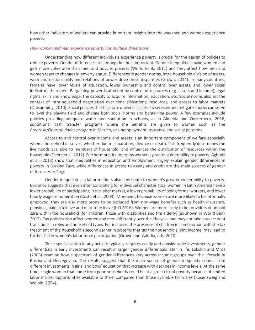
What we find is that girls and young women face a poverty penalty that cannot be explained solely by the characteristics  that are controlled  for, or by the presence of children  in the household. Figure 9 shows how the female poverty penalty, defined as the simple difference between predicted female and 

                                                            

27 As education is age‐dependent, and we are including individuals who might still be in the process of completing their education (e.g. those younger than 25), we choose the highest level of education at the household level instead of individual education. 

20 

 

male  extreme  poverty  rates,  varies  through  the  lifecycle  when  controlling  for  different  individual  and household characteristics. When looking at simple differences without controls, young women suffer from a  sharp  rise  in  the  female  poverty  penalty  between  the  ages  of  20  and  30,  from  about  0.4  to  over  2 percentage  points.  This  penalty  then  falls  and  ultimately  disappears  by  age  40.  Moving  from  the unconditional difference to the base specification that includes country effects and household education slightly  slows  the  increase  in  the  gender  disparity  between  ages  20  and  30.  This  likely  results  from controlling for country dummies, to the extent that poor women in their twenties are disproportionately prevalent in poorer countries, where young women face larger penalties in absolute terms. Controlling for household dependency ratio confirms that the pronounced spike in the female poverty penalty between the ages of 20 and 30 is due to the increased presence of young children. In this specification, however, girls and young women still face a 0.5 to 1 percentage point higher poverty rate between the ages of 0 and 15. Furthermore, when controlling for the individual’s economic activity, women are a full percentage point more likely to be poor than men, all the way from birth until age 45. This is consistent with a higher share of men entering the labor force, and that labor force participation lifting more men than women out of poverty,  particularly  between  the  ages  of  15  and 19.  To  sum up,  there  is  an  observed  female  poverty penalty, which increases with age and peaks at the 20‐30 age group. Part of the sharp increase is due to the presence of young children; however, across all specifications we can observe a poverty penalty of 0.5 to 1 percentage point on girls and young women ages 0 to 15.  

 

Figure 9. Difference between female and male poverty rates (poverty penalty), by age group and specification  

 

Source: WB Staff’s calculations based on GMD. Notes: The Y axis represents the difference between predicted extreme poverty rates for women and men by age group, based on separate r. Sample of 71 countries 

Household Type and Gender: Looking beyond headship 

Lessons  from  the  individual‐level  analysis  indicate  that  household  composition,  particularly  the presence of dependents like young children, plays an important role when it comes to looking at gender differences in poverty through the lifecycle. In this section, we further explore household characteristics and  composition  to  expand  on  gender  differences  when  it  comes  to  poverty. We  seek  to  expand  on 

‐2.0

‐1.0

0.0

1.0

2.0

3.0

0‐4 5‐9 10‐1415‐1920‐2425‐2930‐3435‐3940‐4445‐4950‐5455‐5960‐6465‐6970‐7475‐79 80+

Percentage points

Age groupUnconditionalBase specificationBase plus dependency ratioBase plus dependency ratio and economic activity

21 

 

traditional headship measures, which have proved to be of limited use, to new ways of looking at household composition that might be more informative28. 

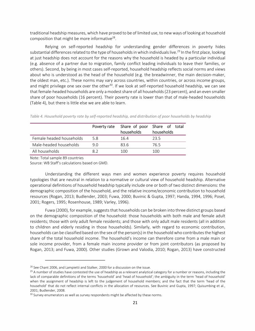
Relying  on  self‐reported  headship  for  understanding  gender  differences  in  poverty  hides substantial differences related to the type of households in which individuals live.29 In the first place, looking at just headship does not account for the reasons why the household is headed by a particular individual (e.g. absence of a partner due to migration, family conflict  leading  individuals to  leave their families, or others). Second, by being in most cases self‐reported, household headship reflects social norms and views about who is understood as the head of the household (e.g. the breadwinner, the main decision‐maker, the oldest man, etc.). These norms may vary across countries, within countries, or across income groups, and might privilege one sex over the other30. If we look at self‐reported household headship, we can see that female‐headed households are only a modest share of all households (23 percent), and an even smaller share of poor households (16 percent). Their poverty rate is lower than that of male‐headed households (Table 4), but there is little else we are able to learn. 

 Table 4. Household poverty rate by self‐reported headship, and distribution of poor households by headship 

  Poverty rate  Share  of  poor households 

Share  of  total households 

Female headed households  5.8  16.4  23.5 

Male‐headed households  9.0  83.6  76.5 

All households  8.2  100  100 

Note: Total sample 89 countries Source: WB Staff’s calculations based on GMD. 

 Understanding  the  different  ways  men  and  women  experience  poverty  requires  household 

typologies that are neutral in relation to a normative or cultural view of household headship. Alternative operational definitions of household headship typically include one or both of two distinct dimensions: the demographic composition of the household, and the relative income/economic contribution to household resources (Rogan, 2013; Budlender, 2003; Fuwa, 2000; Buvinic & Gupta, 1997; Handa, 1994, 1996; Posel, 2001; Rogers, 1995; Rosenhouse, 1989; Varley, 1996).  

Fuwa (2000), for example, suggests that households can be broken into three distinct groups based on the demographic composition of the household: those households with both male and female adult residents; those with only adult female residents; and those with only adult male residents (all in addition to  children  and  elderly  residing  in  those  households).  Similarly,  with  regard  to  economic  contribution, households can be classified based on the sex of the person(s) in the household who contributes the highest share of the total household income. The household’s income can therefore come from a male main or sole  income provider,  from a  female main  income provider or  from  joint  contributors  (as proposed by Rogan, 2013; and Fuwa, 2000). Other studies (Grown and Valodia, 2010; Rogan, 2013) have constructed 

                                                            

28 See Chant 2006, and Lampietti and Stalker, 2000 for a discussion on the issue. 29 A number of studies have contested the use of headship as a relevant analytical category for a number or reasons, including the lack of comparable definitions of the terms ‘household’ and ‘head of household’; the ambiguity in the term ‘head of household’ when  the  assignment  of  headship  is  left  to  the  judgement  of  household members;  and  the  fact  that  the  term  ‘head  of  the household’ that do not reflect internal conflicts in the allocation of resources. See Buvinic and Gupta, 1997; Quisumbing et al., 2001; Budlender, 2008. 30 Survey enumerators as well as survey respondents might be affected by these norms. 

22 

 

“hybrid” compositions trying to capture both the presence and gender of earners and the demographic composition of those who are financially dependent in the household; one such designation is, for example, the “dual‐earner” household meaning a married couple with dependent children. Based on the alternative definitions  proposed  in  the  literature,  we  explore  two  household  classifications,  a  demographic‐based classification and an economic‐based classification. The demographic classification, is based on the adult composition of the household. This typology uses the demographic characteristics of the household, taking as  a  starting  point  the  age  and  sex  of  the  adults  that  live  in  the  household  (defining  adults  as  those individuals of ages between 18 and 64), and distinguishing separate categories for elderly or seniors (those of age 65 or above), and households with dependent children (younger than 18).  

The second classification, takes the economic characteristics of the household as a starting point, namely the presence and sex of all earners in the household. Earners are defined as any individual of age 15 or more that is engaged in economic activity. Households are then classified based on the presence of both earners and non‐earner members who depend on the income earners (understanding as no earners children younger than 18, seniors 65 or older, and/or household members 15‐64 who are not engaged in economic activity).  

Both  classifications  are  summarized  in  Table  5.  In  both  cases, marital  status  is  included  in  the specific analysis of some sub‐groups such as adult couple (which distinguishes between married couples and other multiple adult households) in demographic terms, or couple‐earner (vs. other multiple earner households), in economic composition terms.  Table 5. Household composition typologies 

Demographic  Composition:  Sex  and  number  of adults (18‐64) in the household 

Economic Composition: Sex and number of income earners (15+) in the household  

One adult female  One female earner 

One adult male   One male earner 

Two adults of opposite sex  Married or cohabiting couple Other two adult combinations 

Two earners of opposite sex Couple earner Other two earners combination 

Multiple adult households ‐ Married or cohabiting couple and other adults ‐ Multiple adults  

Multiple earners household ‐ ‐ couple earner and other earners  ‐ Other multiple earner 

Only seniors (65+)  No earners 

Only children (‐18) 

Demographic household composition 

Looking at poverty status through the lenses of the demographic household typology shows that adult couple households (two adults of opposite sex who are married or cohabiting) with children are the largest share of poor households. These households are also overrepresented among the poor (meaning the share among poor households is higher than the share they represent among all households). These households represent 30.6 percent of all households, yet they account for 41.5 percent of households living in poverty (figure 10). Furthermore, adult couple households with children and other adults (i.e. extended family households), account for the second largest share among poor households (28.2 percent) and they are also overrepresented among the poor making up 17 percent of the total households in the sample. On 

23 

 

the other hand, adult couple households without children, are less likely to be poor. Their share among the poor is only 2 percent (compared with 8 percent of all households).  

Adult  couple households with  children,  and adult  couple households with  extended  family  and children, together account for 70 percent of poor households. Sole female adult households with children are only 6 percent of poor households, which is double their share of total households.  

 

Figure 10. Distribution of poor households by demographic household typology  

 Note: Numbers in parenthesis refer to the share of each type in the total number of households. Total sample 89 countries Source: WB Staff’s calculations based on GMD. 

 

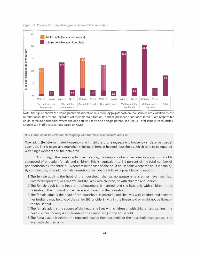
The  demographic  household  classification  clearly  indicates  that  the  presence  of  children  in  a household makes a difference in terms of poverty rates. Figure 11 highlights the demographic composition in a more aggregate fashion, focusing on the presence of children in relation to the adult composition of the household. Overall, households with children tend to fare worse than those without, regardless of the sex, age and/or the number of adults present  in the household. Furthermore, the gaps in poverty rates between presence and absence of children are rather large for all groups. The graph shows two additional points. First, that households with one man and one woman and no other adults mainly consist of couples (married or cohabiting) and their children. Second, it shows that for the case of households with only one adult, those where that adult is the “sole‐responsible” individual in the household (a woman in the majority of cases) make up the largest share of poor households (Box 1 provides more details on this specific group). 

 

   

24 

 

Figure 11. Poverty status by demographic household composition 

 Note: the figure shows the demographic classification in a more aggregate fashion; households are classified by the number of adults present (regardless of their marital situation), and the presence or not of children. “Sole‐responsible adult” refers to households where the one adult is likely to be a single parent (see Box 1). Total sample 89 countries Source: WB Staff’s calculations based on GMD. 

 

Box 1. One adult‐households: Untangling who the “sole‐responsible” adult is. 

One  adult  (female  or  male)  households  with  children,  or  single‐parent  households,  deserve  special attention. This is especially true when thinking of female‐headed households, which tend to be equated with single mothers and their children.  

According to the demographic classification, the sample contains over 7 million poor households composed of one adult female and children. This is, equivalent to 6.1 percent of the total number of poor households (the share is 1.6 percent in the case of one‐adult households where the adult is a male). By construction, one‐adult‐female households include the following possible combinations: 

1. The  female  adult  is  the head of  the household,  she has no  spouse  ‐she  is  either never married, 

divorced/separated, or a widow, and she lives with children, or with children and seniors. 

2. The female adult  is the head of the household,  is married, and she  lives only with children in the 

household; the husband or partner is not present in the household. 

3. The female adult is the head of the household, is married, and she lives with children and seniors; 

her husband may be one of the senior (65 or older) living in the household or might not be living in 

the household 

4. The female adult is the spouse of the head, she lives with children or with children and seniors; the 

head (i.e. her spouse) is either absent or a senior living in the household, 

5. The female adult is neither the reported head of the household, or the household head spouse; she 

lives with children only. 

11.2

2.0

13.5

2.4

15.4

2.4

12.5

1.8

18.0

3.1

20.4

3.2

8.2

0

5

10

15

20

25

With ch No ch With ch No ch With ch No ch With ch No ch With ch No ch With ch No ch

One male and onefemale only

Other adultscombinations

One adult, female One adult, male Multiple adults,only female

Multiple adults,only male

Total

% of poor households by typology

Sole‐responsible adult household

Adult couple (i.e. married couple)

25 

 

6.  The female adult is neither the household head nor has a spouse; she lives with children and seniors; 

the head of the household may be a senior. 

For the purposes of the analysis, we have defined as sole‐responsible adult households those where the one adult (i) lives with children only (no seniors in the household) because, regardless of whether she is the head or is married, the spouse is not reported to be living in the household; or ii) is the head, has no spouse, and lives with children, or children and seniors, because the seniors most likely depend on her, and the senior is not a spouse (it is worth noting that households with senior members and children are 0.7 percent of all poor households). By this definition, of the 7 million of one‐adult‐female with children households  that are poor, 81 percent are sole‐responsible adult ones.  In  the case of one‐adult‐male households with  children  that  are  poor,  83  percent  correspond  to  sole‐responsible  ones. While  the difference is not large, it indicates how difficult is to define headship and household responsibility. 

 

 The demographic household composition analysis by regions reveals  important variations in the 

shares of poor households in each group across regions. Numbers confirm that adult couple households with children, and with children and other adults (extended family), are the most common household type across all regions, and that they are the most frequent group to be found among poor households (Table 6). However, there are other types of households that gain relevance depending on the region. One adult female households with children are more prevalent among the poor in Latin America and the Caribbean and  in Sub‐Saharan Africa than  in other regions but they are  less prevalent among the total number of households.  

In East Asia and the Pacific, and Europe and Central Asia, a non‐negligible share of poor households are adult couple (e.g. married or cohabiting) households without children (4 percent). In Europe and Central Asia, extended family households (adult couple households with children and other adults) are more likely to be poor than the adult couple households with children and no other adults. In all other regions, the reverse is true. Finally, one adult households without children, regardless of the sex of the adult, constitute an important share of the poor (as well as an important share of the total number of households) in Latin America and the Caribbean and in Europe and Central Asia.  Table 6. Distribution of demographic household types across regions (poor households) 

HOUSEHOLD TYPE  Region 

EAP  ECA  LAC  SAR  SSA 

One adult, female ‐ no children  2.0%  2.9%  4.7%  1.1%  0.9% 

One adult, female ‐ with children  2.6%  2.3%  14.0%  3.2%  8.4% 

One adult, male ‐ no children  2.1%  7.7%  7.6%  0.7%  1.1% 

One adult, male ‐ with children  1.6%  0.4%  2.1%  0.7%  2.3% 

Adult couple ‐ no children  3.8%  3.8%  3.8%  1.7%  1.3% 

Adult couple ‐ with children  32.6%  20.4%  34.2%  44.3%  43.0% 

Adult couple ‐ with children and other adults  28.8%  34.3%  12.4%  32.6%  26.3% 

Multiple adults no children  1.2%  1.3%  2.1%  0.3%  0.7% 

Multiple adults, only female ‐ with children  1.1%  1.2%  3.7%  1.2%  3.5% 

Multiple adults, only male ‐ with children  0.3%  0.1%  0.5%  0.3%  1.1% 

26 

 

Adults combinations (other than a couple) ‐ no children  9.4%  7.9%  4.0%  3.9%  2.3% 

Other adult combinations ‐ with children  6.8%  15.8%  5.9%  7.8%  6.9% 

Senior(s) only ‐ no children  6.9%  1.8%  4.0%  1.7%  0.8% 

Senior(s) only ‐ with children  0.7%  0.0%  0.6%  0.1%  1.3% 

No adults, children only  0.0%  0.2%  0.3%  0.4%  0.1% 

Total  100%  100%  100%  100%  100% 

Note: Total sample 89 countries Source: WB Staff’s calculations based on GMD. 

Economic household composition 

The economic household composition assumes that a household member can be classified in one of two categories: as an  income earner, meaning an  individual 15 or older who is engaged  in economic activity for pay, or a non‐earner member, namely, those who depend on the income earners and/or depend on other income transfers such as social protection programs or remittances, for example. To differentiate on the type of  income dependent, we distinguish between earner dependent, those non‐earners 18‐64, and other dependents which follows the traditional definition of children (younger than 18) and/or seniors (65 or older) who, are distinguished among the non‐earners from the adults. (See Box 2 for more details about the non‐earners). 

 Box 2. Child and senior breadwinners and non‐earner members 

According to the definitions above, children 15‐17 and seniors 65+ can fall in either the earner or non‐earner category. The more traditional definition of working age population covers those 15‐64 (above legal age for work and below retirement age). For the case of this analysis we are  including a wider definition covering those 15 and above.  

In the case of youth ages 15‐17, the GMD contains over 243 million people of which 52 percent are boys and 48 percent girls. The majority (70 percent) report going to school, 13 percent are not in school or employed, 10 percent are engaged in paid work, and 6 percent are engaged in unpaid work. Of those engaged in paid work 68 percent are boys, who also make the majority of those un unpaid work. Among those who live in poor households, 28 percent of young girls and boys are engaged in economic activity. 8 percent of girls, and 14 percent of boys who live in poor households are engaged in paid work.  

These figures translate in: Households with children 15‐17 as the only earners are a very small share of all households (0.3 percent). Households with seniors 65+ as the only earners are only 2 percent of all households. 4.3 percent of households have among their earners someone 65 or older (this number is slightly higher among poor households at 5.5 percent). Earners are concentrated mainly in the 18‐64 age group. 

The economic definition refers to earners as those who contribute with monetary income from paid work. It is important to acknowledge that some non‐earners, are engaged in economic activity as unpaid workers or  through contributions  in‐kind to  the household. For example,  they may engage  in work that is not visible or accounted for as work such as unpaid domestic work.  

One clear example of unpaid domestic work is found in households where women take care of children and/or the elderly. Examples of such households are (i) households with a male earner, a non‐earner  spouse, and children/senior dependents;  (ii) households with a  female non‐earner, an earner spouse, and children/senior dependents; (iii) households with a male earner, without spouse, and with 

27 

 

adult non‐earners, and children/seniors, since  it may be  that one non‐earner adult  female does care work.  

 

The analysis of poverty by the economic characteristics of the household, confirms the previous findings that households with traditional dependents (children younger than 18 and/or seniors 65 and older (Figure  12))  fare  worse  than  households  without  dependents.  And,  in  most  cases,  having  an  earner dependent  (i.e.  household members  18‐64 who  are  non‐income‐earners)  also  increases  poverty  rates (Figure 12). Households with an absence of an earner,  combined with  the presence of children and/or seniors, are the poorest type household (23.5 percent live in poverty), followed by households with a single female  earner  and  dependents  (16.8  percent  live  in  poverty).  Female  single  earner  households  with dependents of any type are also over‐represented among poor households. They represent 5.5 percent of all households, but 7.9 percent of poor households.  

 Figure 12. Poverty rate by economic household composition  

 Note: Sample of 71 countries. Head couple earner refers to married/cohabiting earners. Source: WB Staff’s calculations based on GMD. 

 

Figure 13 presents a more disaggregated version of  the economic composition.  It distinguishes between non‐earners who are children, seniors, earner dependents (aged 18‐64), or a combination of any of these. The distribution of poor households shows that multiple individual households that include adults who are not actively engaged in economic activity (non‐earners), and dependents, all depending on a single male earner, constitute the largest share of poor households. This result is consistent with the results from the demographic composition, in which extended family households are one of the most prevalent types among  poor  households,  and  are more  frequent  among  the  poor  than  the  non‐poor.  Extended  family households represent 21 percent of all households, yet they account for 36.2 percent of households living in poverty. Households with dependents and no earners are the second most common type among poor households. They represent 5 percent of all households but 14 percent of poor households.  

16.8

13.4

7.5

7.1

11.7

23.5

15.0

8.5

6.1

15.3

9.8

9.0

10.0 5.0 0.0 5.0 10.0 15.0 20.0 25.0

Single female earner

Single male earner

Head couple earner

2 earners different sex

Multiple earners

No earners

w/o earner dep w/o other dep w/o earner dep with other dep

with earner dep w/o other dep with earner dep with other dep

28 

 

The share of extended family households living in poverty is eight times that of a similar type of household without dependents (16.8 vs. 2.1 percent). This difference also holds for the case of poor male single‐earner households with earner dependents, where the poverty rate for those with dependents is six times that of those without dependents. On the other hand, households with a head‐couple earner (a male and female earner, married or living together, with no other adults) are less likely to be poor. Although in their case, the presence of dependents also affects the level of poverty negatively. 

In general, the presence of dependents increases the share of each earner composition household among the poor (regardless of presence, sex or number of earners), in line with finding of the demographic composition. The combination of children and non‐earner adults (with or without seniors) is the one that matters the most. In fact, households with this combination of dependents represent 72.5 percent of poor households (but less than half of all households), as opposed to households where dependents are only non‐earner adults which make up only 6 percent of poor households, or where the dependents are only seniors which make up 4 percent of poor households.31  

 As  with  the  demographic  composition,  we  observe  variation  across  regions  in  the  types  of 

households that are more prevalent among the poor (Table 7). Even though sole female earner households are less frequent among the poor in the aggregate, they make up the largest share of poor households in Latin  America  and  the  Caribbean  and  Sub‐Saharan  Africa,  particularly  if  they  have  children  and  other dependents (7 and 8 percent respectively). The most frequent household type varies by region. The largest group is households with a male earner, children and other dependents (particularly an earner dependent, typically a spouse or cohabiting partner). This group ranges from over half of all poor households in South Asia, to about 25 percent of all households in the other regions. The second largest group in terms of share of  poor  households  is  households with  dependents  but  no  earners.  These  households where  no  labor income earner is reported, but that may include unpaid or contributing family workers or receive social transfer  or  remittances,  represent  48  percent  of  poor  households  in  Latin  America  and  the  Caribbean (compared to only 2 percent of all households in that region), and 37 percent of poor households in Europe and Central Asia (where two thirds are senior individuals’ households which probably have pensions as their main income source). In Sub‐Saharan Africa, the share of no‐earner households among the poor is larger than male earner households with dependents, and, as  in Latin America, most of  these households are composed by children and non‐earners 15‐64. For South Asia, the second largest household type among the poor is multiple earners households with dependents (18 percent). 

   

                                                            

31 In the aggregate, households with dependents who are seniors (no children) represent a higher share of total households (10.4 percent), so do households where dependents are non‐earner adults only (17.4 percent); households with children and non‐earner adults represent a lower share in the aggregate (42.1 percent)) than among the poor households (72.5 percent) which means this typology is overrepresented among the poor. 

29 

 

Figure 13. Distribution of poor households by economic household typology  

 Note: Numbers in parenthesis refer to the share of the typology in the total number of households. Distribution graph shows typologies that represent at least 1% of total poor (IPL) households only. Sample of 71 countries Source: WB Staff’s calculations based on GMD. 

 

Table 7. Distribution of economic household typologies across regions (poor households) 

Household Type  Region 

EAP  ECA  LAC  SAR  SSA 

Female earner with children only  0.4%  0.4%  2.5%  1.0%  3.8% 

Female earner with children and other dependents  3.8%  6.4%  6.9%  1.9%  8.4% 

Female earner with earner dependent only  0.5%  2.9%  1.0%  0.1%  0.4% 

Male earner with children only  0.9%  0.3%  0.3%  0.1%  0.4% 

Male earner with children and other dependents  25.2%  23.3%  26.2%  53.0%  26.0% 

Male earner with earner dependent only  2.4%  4.9%  2.2%  2.5%  1.2% 

Head couple with children only  4.8%  2.0%  2.0%  5.5%  11.7% 

Head couple with children and other dependents  6.0%  1.4%  1.7%  4.0%  6.5% 

Head couple with earner dependent only  0.2%  0.8%  0.1%  0.1%  0.2% 

Multiple earners with children only  5.8%  0.2%  0.5%  2.1%  3.1% 

Multiple earners with children and other dependents  12.4%  6.4%  2.8%  18.1%  5.6% 

Multiple earners with earner dependent only  2.3%  1.3%  0.3%  1.6%  0.3% 

No earners with dependents   17.7%  37.1%  48.0%  3.8%  27.1% 

Two earners different sex with dependents  3.6%  2.5%  1.1%  2.3%  1.8% 

30 

 

Any earner type with no dependents  7.5%  5.4%  2.0%  1.5%  2.5% 

Any earner type with senior dependent   6.7%  4.6%  2.4%  2.5%  1.0% 

Total  100%  100%  100%  100%  100% 

Note. Some groups have been collapsed for presentation purposes. Sample of 71 countries Source: WB Staff’s calculations based on GMD. 

 

In which types of households do poor women live? 

Results at the individual level, show that by age 20 to age 34, women are two percentage points poorer than men, which is a significant difference. At the household level, adult couples with children and single male earner with children and a non‐earner dependent are the most numerous among the poor. At the individual level, marriage is the most frequent status for women in the 20‐34 age group. 

 All  these  findings  suggest  household  formation  and  income  generation  are  possible  factors associated with individuals living in a poor household. In fact, both poor and non‐poor women concentrate in the adult couple household with children (with or without other adults) group. However, the share of women living in households with children is higher among poor women (more than 90 percent) than among non‐poor counterparts (75 percent of total non‐poor women, and 77 percent among the 20‐34 age group). Similarly, the share of non‐poor women living in households without children is higher than among poor women. Looking through the lenses of the economic composition, more than half of poor and non‐poor women live in households with children and with children and earner dependents, and where the earner is  a  single male  or  a  head  couple.  This  is  also  the  case  among women  20‐34.  As  in  the  demographic composition case, women are concentrated in the most frequent household type found among the poor. Yet, the shares of poor women (both all women and women ages 20‐34) living in households with both children and non‐earner adults (i.e. more members depend on the income earner) is higher than among non‐poor women. 

These patterns also hold  true across  regions, where  the highest  share of poor women  living  in households with children is found in Sub‐Saharan Africa (97 percent, compared to 88 percent among non‐poor women), and the lowest in East Asia and the Pacific (86 percent, compared to 67 percent among non‐poor women). 

 

Table 8. Distribution of poor and non‐poor women by demographic and economic household compositions, global. 

Demographic household typology  All women  Women 20‐34 

Poor  Non‐poor 

Poor  Non‐poor 

Adult couple ‐ with children (30.6%)  38.3%  33.6%  43.0%  37.6% 

Adult couple ‐ with children and other adults (17.1%)  37.6%  28.1%  36.2%  27.8% 

Adult combinations (other than a couple) ‐ without children (13.6%)  2.6%  12.0%  3.6%  13.3% 

One adult only ‐ no children (11.2%)  0.7%  3.3%  0.3%  2.8% 

Total (72.5%)  79.2%  77%  83.1%  81.5% 

 

 

 

31 

 

Economic household typology  All women  Women 20‐34 

Poor  Non‐poor 

Poor  Non‐poor 

Male earner ‐ with children & earner dep (21.0%)  41.7%  28.1%  39.8%  28.2% 

Head couple earner ‐ with children only (10.2%)  10.6%  15.0%  10.4%  14.4% 

Multiple earners ‐ with children & earner dep (7.1%)  15.0%  12.2%  15.0%  13.3% 

No earners ‐ with senior dep (6.7%)  0.9%  4.3%  0.2%  0.3% 

Total (45%)  68.3%  59.5%  65.3%  56.2% 

Note: Numbers in parenthesis refer to the share of each typology in the total number of households; table shows the four typologies with the highest shares among total households. Sample of 89 countries for Demographic typology, and 71 countries for Economic Typology Source: WB Staff’s calculations based on GMD. 

 

The  previous  sub‐sections  examined  the  share  of  different  types  of  households  that  are  poor, classified both according to their demographic and economic composition. On the demographic side,  in general households with  children  are more  likely  to be poor  than  similar households without  children. However, of the households with children, the most common types of households ‐‐ those with children and  an  adult  couple,  with  or  without  other  adults  present  ‐‐  have  a  smaller  share  in  poverty.  On  the economic side, households with both adult and child dependents are disproportionately poor, particularly those with no earners, a single female earner, or to a lesser extent, a single male earner. Among households without grown dependents, single female earner households are the poorest.  

This  final  section  considers  the  extent  to  which  these  results  are  robust  when  controlling  for additional characteristics. For each type of classification, we consider three specifications. The first contains no controls and therefore reflects the unconditional  relationship between household type and extreme poverty. These are equivalent to the unconditional results presented at the individual  level. The second controls for a full set of country dummy variables, and therefore only considers within‐country variation in poverty  and  household  type.  The  third  specification  adds  four  additional  household  characteristics  as controls: the maximum educational attainment category, the average age of earners, and household size, and an urban/rural dummy. As can be seen in Figure 14 below, adding even country dummies significantly attenuates the differences in poverty between the different types of household that contain children. With the full set of controls, single female adults with children are the poorest,  followed by households with children and multiple female or male adults. The differences  in poverty rates between households with children and without remains, but is reduced, to about 2 to 3 percentage points (results shown in annex, Tables A7 and A8). 

With respect to the economic classification (Figure 15), introducing controls also greatly reduces the  penalty  for  household  types  with  both  adult  and  traditional  dependents  (children  an  elderly). Nonetheless,  the  penalty  for  these  types  of  households  remains  larger  than  for  others,  except  for households with one male earner and both earner dependents and traditional dependents. Controlling for other characteristics, 9.8 percent of households with a one female earner and traditional dependents, but no adult dependents, are poor. This is close to the 11 percent share for households with no earners and both  adult  and  traditional  dependents.  This  is  still  significantly  larger  than  other  households  that  are unlikely to be in poverty, such as those with one male earner and traditional dependents, or household couples that both work and support both traditional and earner dependents. Not surprisingly, the economic classification, to a greater extent than the demographic classification, remains an important determinant of household poverty status after controlling for selected household characteristics and country dummies.  

32 

 

Figure 14. Probability of extreme poverty for selected household demographic types by specification 

 

Note: Sample of 89 countries Source: WB Staff’s calculations based on GMD.  

Figure 15. Probability of extreme poverty for selected household economic types by specification 

 

Note: Sample of 71 countries Source: WB Staff’s calculations based on GMD. 

 

 

0%

5%

10%

15%

20%

25%

Male adults,with children

Femaleadults, withchildren

One Femadult, withchildren

Other combo,with children

One maleadult, withchildren

One male onefem, withchildren

Unconditional Within country Within country and controls

0%

5%

10%

15%

20%

25%

No earners, adultdeps, traditional

deps

One female earner,adult deps,

traditional deps

One male earner,adult deps,

traditional deps

One female earner,No adult deps,Traditional deps

Share of households that are poor

Unconditional Within country Within country and controls

33 

 

Conclusions 

This analysis provides a glimpse of  the  richness and  complexity  that  can be  seen  introducing a gender lens to poverty analysis. The findings of this study indicate that incorporating such a lens can provide important  insights  for  policy  design  which  has,  to  date,  not  included  a  systematic  analysis  of  gender differences when it comes to policies to eradicate extreme poverty.  

At the global level, four main findings appear. First, not only does a gender lens matter for poverty analysis in general it also matters in relation to the moment in the lifecycle for women and men (e.g. their marital status, presence of children and dependents in their households, when and if they join the labor market, and the responsibilities for reproductive work).  

Second,  children  and  dependents,  demographically  and  economically,  are  an  important vulnerability  factor particularly  for women during their  reproductive years. Care responsibilities overlap with economically productive years (high labor market participation and best time for income generation years), making women specifically vulnerable due to multiple demands on their time.  

Third, for both men and women, pooling resources, meaning having more adults working for pay in  a  household,  appears  to  be  a  protective  factor  against  poverty.  Formal  education  is  also  a  strong protective factor against poverty, especially for women. 

 Finally, at the household level, no one single element, whether it is self‐declared headship, adult composition,  or  earner  composition,  seems  to  be  enough  to  determine  household‐level  poverty,  so complementary approaches are required to look at household‐level poverty and its main determinants. 

This paper provides important insights based on the exploration of a dataset like the GMD, and it suggests the value of continuing this type of analysis to further understand gender, and other differences within poor and vulnerable households. A clear further research agenda for evidence‐based policy decision‐making  at  the  country  or  regional  level,  leveraging  new data  being  collected  can  build  on  these  initial findings. Among these, expanding from income and consumption based approaches to explore the multi‐dimensions of poverty and how these can vary between women and men is an important one. 

 

 

   

34 

 

References 

Agbodji, Akoété, Yélé Batana, and Dénis Ouedraogo. 2013. Gender Inequality in Multidimensional Welfare Deprivation in West Africa: The Case of Burkina Faso and Togo. Policy Research Working Paper 6522. The World Bank.  

Alkire,  Sabine  and  James  Foster.  2011.  Counting  and  Multidimensional  Poverty  Measurement.  Journal  of  Public Economics 95: 476‐487. 

Alkire, Sabine and Maria Emma Santos. 2014. “Measuring Acute Poverty in the Developing World: Robustness and Scope of the Multidimensional Index.” World Development 59: 251‐74. 

Almeida,  Rita  and  Oosterbeek,  H.  (2016).  Access  to  water  and  sanitation  in  Panamanian  schools  and  student outcomes. Education Global Practice, World Bank, Washington, D.C. 

Anyanwu, John. 2010. “Poverty in Nigeria: A Gendered Analysis”. Journal Statistique Africain, N. 11, Novembre 2010.  

Bardasi,  Elena  and  Quentin Wodon.  2010. Working  Long  Hours  and Having  No  Choice:  Time  Poverty  in  Guinea. Feminist Economics 16 (3): 45‐78. 

Bargain, Olivier, Olivier Donni, and Prudence Kwenda. “Intra‐household distribution and poverty: Evidence from Cote d'Ivoire.” Journal of Development Economics 107 (2014): 262‐276. 

Batana, Yélé. 2013. Multidimensional Measurement of Poverty among Women in Sub‐Saharan Africa. Social Indicators Research 112: 337‐362. 

Bessell, Sylvia. 2010. Methodologies for Gender‐Sensitive and Pro‐Poor Poverty Measures. In Chant, S. (Ed.) (2010). The International Handbook of Gender and Poverty: Concepts, Research, Policy. Cheltenham: Edward Elgar.  

Bessell, Sharon. 2014. The Individual Deprivation Measure: A New Approach to Multi‐Dimensional, Gender Sensitive Poverty Measurement. CROP Poverty Brief, July 2014. 

Bradshaw, S. 2002. Gendered Poverties and Power Relations: Looking inside Communities and Households (Managua: ICD/Embajada de Holanda/Puntos de Encuentro). 

BRIDGE (2001) “Feminisation of Poverty”. Briefing Paper. Brighton: Institute of Development Studies, University of Sussex. 

Brown,  Caitlin, Martin  Ravallion,  and  Dominique  van  de Walle.  2017.  Are  Poor  Individuals Mainly  Found  in  poor Households? Policy Research Working Paper 8001. The World Bank.  

Budlender, Debbie. 2008. The Debate about Household Headship. Social Dynamics 29 (2): 48‐72. 

‐ ‐ ‐. 2005. Women and Poverty. Agenda: Empowering Women for Gender Equity, No. 64  

Buvinic, Mayra and Geeta Gupta. 1997. Female‐headed Households and Female‐Maintained Families: Are They worth Targeting to Reduce Poverty in Developing Countries? Economic Development and Cultural Change 45 (2): 259‐280. 

Castañeda, Andres, Dung Doan, David Newhouse, Minh C. Nguyen, Hiroki Uematsu, João Pedro Azevedo, and Data for Goals Group. 2018. World Development 101: 250‐267. 

Chant, Sylvia  (Ed.). 2010.  International Handbook of Gender and Poverty: Concepts, Research Policy. Cheltenham: Edward Elgar.  

Chant, Sylvia. 2003. Dangerous Equations? How Female‐headed households became the Poorest of the Poor: Causes, Consequences and Cautions. IDS Bulletin 35.4 Repositioning Feminists in Development.  

‐ ‐ ‐. 2003. The “Engendering” of Poverty Analysis in Developing Regions: Progress since the United Nations Decade for Women, and Priorities for the Future. Issue 11 November 2003. 

‐ ‐ ‐. 2003. Female household headship and the feminization of poverty: facts, fictions and forward strategies [online]. London: LSE Research Online. Available at: http://eprints.lse.ac.uk/archive/00000574.  

‐  ‐  ‐.  2006.  Rethinking  the  “Feminization  of  Poverty”  in  Relation  to  Aggregate Gender  Indices.  Journal  of  Human Development 7 (2): 201‐220. 

‐ ‐ ‐. 2008. “The Feminization of Poverty and the ‘Feminization’ of Anti‐Poverty Programmes: Room for Revision?” Journal of Development Studies 44 (2): 165‐197. 

Chiappori, Pierre‐Andre and Costas Meghir. 2014. “Intra‐household Welfare.” NBER Working Paper 20819. National Bureau of Economic Research, Cambridge, MA.  

35 

 

Coudouel, Aline, Jesko S. Hentschel, and Quentin T. Wodon. 2002. “Poverty Measurement and Analysis.” In Klugman, J. (Ed.) (2002). A Sourcebook for Poverty Reduction Strategies. World Bank: Washington, D.C.  

Costa, Joanna, Elydia Silva and Fabio Vaz. 2009. The Role of Gender Inequalities in Explaining Income Growth, Poverty and Inequality: Evidence from Latin American Countries. Working Paper 52. International Policy Centre for Inclusive Growth, United Nations Development Programme.  

Deaton, Angus. 1997. The Analysis of Household Surveys: A Microeconometric Approach to Development Policy. World Bank, Washington, D.C.  

Deere, Carmen, Gina Alvarado, and Jennifer Twyman. 2012. Development and Change 43 (2): 505‐530.  

Dercon, Stefan and Pramila Krishnan. 2000. In Sickness and in Health: Risk Sharing within Households in Rural Ethiopia. Journal of Political Economy 108 (4): 688‐727. 

Dunbar,  Geoffrey  R.,  Arthur  Lewbel,  and  Krishna  Pendakur.  “Children's  resources  in  collective  households: identification,  estimation,  and  an  application  to  child  poverty  in Malawi.”  The  American  Economic  Review  103.1 (2013): 438‐471. 

Economic Commission for Latin America and the Caribbean. 2016. Equality and Women’s Autonomy in the Sustainable Development Agenda. United Nations. Santiago 

Gaddis, Isis. 2016. “Individual Poverty Measurement.” Submission to the Commission on Global Poverty. Mimeo.  

Gideon, Jasmine. 2010. Poverty, Gender and the Right to Health: Reflections with Particular Reference to Chile.  In Chant, S. (Ed.) (2010). The International Handbook of Gender and Poverty: Concepts, Research, Policy. Cheltenham: Edward Elgar. 

Grown, Caren. 2014. Missing Women: Gender and the Extreme Poverty Debate. A paper prepared for USAID under Award #AIDOAA‐ 0‐13‐00103 Mod 1. 

Grown, Caren and Valodia, Imraan (Eds.). 2010. Taxation and Gender Equity: A Comparative Analysis of Direct and Indirect Taxes in Developing and Developed Countries. International Development Research Centre. 

Fuwa, N. (2000a). A note on the analysis of female‐headed households in developing countries. (Technical Bulletin, pp. 125–138). Chiba: Faculty of Horticulture of Chiba University. 

‐‐‐‐‐‐‐‐‐‐. (2000b). The poverty and heterogeneity among female‐headed households revisited: The case of Panama. World Development, 28(9), 1515–1542. 

Haddad, Lawrence, and Ravi Kanbur. 1990. How Serious is the Neglect of Intra‐Household Inequality.? The Economic Journal 100 (402), September 1990.  

Klasen, Stefan, Tobias Lechtenfeld, and Feliz Povel. 2015. A Feminization of Vulnerability? Female Headship, Poverty, and Vulnerability in Thailand and Vietnam. World Development 71: 36‐53. 

Lambert, Sylvie, Martin Ravallion and Dominique van de Walle. 2014. Intergenerational Mobility and Interpersonal Inequality in an African Economy. Journal of Development Economics 110: 327‐344. 

Lanjouw,  Peter.  2012.  Counting  Women  in  Poverty:  Potential  Pitfalls  in  Conventional  Poverty  Analysis.  PREM Knowledge and Learning Weeks. World Bank, May 2008. 

Lokshin, Michael  and  Thomas A. Mroz.  2003.  “Gender  and Poverty:  A  Life  Cycle  Approach  to  the Analysis  of  the Differences in Gender Outcomes.” World Bank Policy Research Working Paper 3153.  

Lundberg, Shelly J., Robert A. Pollak, and Terence J. Wales. 1997. “Do Husbands and Wives Pool Their Resources? Evidence from the United Kingdom Child Benefits.” Journal of Human Resources 32(3): 436‐80. 

Newhouse, David, Pablo Suárez Becerra, and Martin Evans, 2017, "New global estimates of child poverty and their sensitivity to alternative equivalence scales." Economics Letters 157: 125‐128. 

Quisumbing, Agnes, Lawrence Haddad, and Christine Peña. 2001. Are Women Overrepresented Among the Poor? An Analysis of Poverty in 10 Developing Countries. Journal of Development Economics 66: 225‐269. 

Quisumbing, Agnes  (Ed.).  2003. Household Decisions, Gender  and Development: A Synthesis of Recent Research. Washington, DC: International Food Policy Research Institute.  

‐ ‐ ‐. 2010. Gender and Household Decision‐Making in Developing Countries: A Review of Evidence. In Chant, S. (Ed.) (2010). The International Handbook of Gender and Poverty: Concepts, Research, Policy. Cheltenham: Edward Elgar. 

36 

 

Ravallion, Martin. 2011. “On Multidimensional Indices of Poverty.” Journal of Economic Inequality 9: 235‐248. 

Rogan, Michael. 2012. Poverty and Headship in Post‐Apartheid South Africa, 1997‐2008. ERSA Working Paper 288.  

‐ ‐ ‐. 2013. Alternative Definitions of Headship and the ‘Feminization’ of Income Poverty in Post‐Apartheid in South Africa. The Journal of Development Studies 49 (10): 1344‐1357.  

Rosenzweig, Mark and Kenneth I. Wolpin. 1994. “Are There Increasing Returns to the Intergenerational Production of Human Capital? Maternal Schooling and Child Intellectual Achievement.” Journal of Human Resources 29 (2): 670‐693. 

Sen, Gita. 2010. Poor Households or Poor Women: Is There a Difference? In Chant, S. (Ed.) (2010). The International Handbook of Gender and Poverty: Concepts, Research, Policy. Cheltenham: Edward Elgar.  

United Nations. 2015. Integrating a Gender Perspective into Statistics. New York: UN Department of Economic and Social Affairs, Statistics Division.  

‐ ‐ ‐. 2015. The World’s Women 2015. New York: UN Department of Economic and Social Affairs, Statistics Division.  

Wisor, Scott. 2011. Poverty Measurement: What’s Gender Got to Do with It? Rethinking Development in an Age of Scarcity and Uncertainty.  

World Bank. 2011. World Development Report 2012: Gender Equality and Development. Washington D.C: World Bank.  

‐ ‐ ‐. 2015. A Measured Approach to Ending Poverty and Boosting Shared Prosperity: Concepts, Data, and the Twin Goals. Policy Research Report. Washington, D.C: World Bank. 

‐ ‐ ‐. 2017. Monitoring Global Poverty: Report of the Commission on Global Poverty. Washington, D.C: World Bank. 

37 

 

Annexes  

Table A1: Creation of the final sample GMD    Table A2: Characteristics of the final sample GMD 

 Number of countries 

Number of surveys 

Number of households* 

Number of individual records* 

   Number of countries 

Population Share of sample population 

GMD sample   89  104  2,055,717  7,649,676    Total*  71  4,835,078,613  100% 

Primary activity reported for 70% of observations  

84  99  1,986,637  7,337,596    Income Group 

Primary activity consistent with employment status  

82  97  1979442  7,302,438    Low Income   13  337,990,810  7.0% 

Share of adults out of labor force 10% >100%  

76  91  1918371  7,023,895   Lower Middle Income 

25  2,241,252,372  46.4% 

Employment status distinguishes between unpaid, paid, and self‐employed  

71  86  1865369  6,799,153   Upper Middle Income 

20  1,988,304,246  41.1% 

Note: * weighted sample  Source: Global Micro Database, authors’ calculations  

  High income  13  267,531,185  5.5% 

  Region 

  East Asia & Pacific  10  1,882,772,025  38.9% 

 Europe and Central Asia 

18  382,406,458  7.9% 

 Latin America & Caribbean 

17  539,821,384  11.2% 

 Middle East & North Africa 

3  16,288,184  0.3% 

  South Asia  5  1,460,853,641  30.2% 

 Sub‐Saharan Africa 

18  552,936,921  11.4% 

  Welfare Type 

  Consumption  42  4,093,499,010  84.7% 

  Income  29  741,579,603  15.3% 

     

 

 

38 

 

Table A3. Poverty rate by sex and geographic area 

Region  Female  Male 

  Urban  Rural   Urban  Rural  

East Asia and Pacific  1.9  5.3  1.8  5.2 

Europe and Central Asia  0.4  1.5  0.4  1.5 

Latin America and Caribbean  3.4  13.3  3.0  12.8 

South Asia  9.4  18.6  8.3  17.4 

Sub‐Saharan Africa  25.0  52.3  24.3  51.9 

Total  5.7  18.7  5.4  17.9 

Note: 89 countries Source: WB Staff’s calculations based on GMD. 

 

Table A4. Femininity index by age group and region 

   0‐4 

5‐9 

10‐14 

15‐19 

20‐24 

25‐29 

30‐34 

35‐39 

40‐44 

45‐49 

50‐54 

55‐59 

60‐64 

65‐69 

70‐74 

75‐79 

80+ 

East Asia and Pacific  0.94  1.01  0.99  1.03  1.00  1.13  1.07  0.95  1.01  0.91  1.20  1.01  0.99  1.05  0.80  1.12  1.00 

Europe and Central Asia  1.23  1.06  1.19  1.11  1.26  1.05  1.15  0.83  0.79  0.94  1.02  0.95  0.87  0.67  0.60  0.80  0.48 

Latin America and Caribbean  0.98  0.99  1.04  1.11  1.26  1.35  1.28  1.16  1.09  0.95  1.02  0.85  0.93  1.02  0.92  1.06  0.91 

South Asia  1.10  1.10  1.11  1.14  1.24  1.20  1.17  0.97  0.89  0.84  1.09  1.12  1.25  1.03  0.90  1.19  0.83 

Sub‐Saharan Africa  1.02  0.98  0.97  0.91  1.11  1.28  1.26  1.13  1.05  0.96  0.88  0.82  0.80  0.73  0.83  0.87  0.87 

Total  1.06  1.05  1.04  1.02  1.17  1.24  1.21  1.03  0.98  0.90  1.02  0.98  1.02  0.92  0.84  0.95  0.79 

Note: 89 countries Source: WB Staff’s calculations based on GMD. 

 

 

   

39 

 

Table A5. Poverty rates and distribution of the poor by sex and age group 

a. Poverty rates 

  Female poverty rate  Male poverty rate 

   0‐14  15‐24  25‐34  35‐39  40‐49  50‐54  55‐59  60+  0‐14  15‐24  25‐34  35‐39  40‐49  50‐54  55‐59  60+ 

East Asia and Pacific  5.8  3.4  3.2  3.1  2.5  2.7  2.9  3.3  5.9  3.4  2.9  3.3  2.6  2.2  2.9  3.3 

Europe and Central Asia  1.6  1.1  0.8  0.6  0.5  0.4  0.4  0.2  1.4  1.0  0.7  0.7  0.6  0.4  0.4  0.4 

Latin America and Caribbean  8.4  5.8  5.0  4.7  3.9  3.7  3.1  2.8  8.4  4.9  3.8  4.1  3.8  3.7  3.7  2.9 

South Asia  22.1  14.2  15.0  14.1  11.3  10.8  11.1  12.4  20.0  12.0  12.7  14.6  12.9  9.9  10.0  11.6 

Sub‐Saharan Africa  49.3  38.9  40.9  42.7  40.9  36.7  32.6  32.1  49.5  39.5  32.1  37.7  40.4  41.5  39.5  40.1 

Total  21.2  12.7  11.6  10.5  7.9  7.2  6.8  6.7  20.1  11.7  9.4  10.1  8.4  7.1  7.0  7.3 

 

b. Distribution of the poor, by sex, region and age group 

  Female  Male 

   0‐14  15‐24  25‐34  35‐39  40‐49  50‐54  55‐59  60+  0‐14  15‐24  25‐34  35‐39  40‐49  50‐54  55‐59  60+ 

East Asia and Pacific  31.2  14.9  14.1  6.7  11.5  4.8  4.4  12.4  34.1  15.2  12.8  7.0  11.7  3.9  4.2  11.0 

Europe and Central Asia  36.2  19.3  15.8  5.8  8.4  3.9  3.7  6.9  35.1  18.1  15.8  7.2  10.1  3.6  3.5  6.6 

Latin America and Caribbean  39.8  18.3  15.0  6.3  8.9  3.6  2.5  5.7  44.5  17.3  12.2  5.6  8.9  3.5  2.8  5.2 

South Asia  41.8  16.8  15.4  6.0  7.9  3.0  2.6  6.4  42.2  15.7  14.1  6.7  9.9  3.0  2.5  5.8 

Sub‐Saharan Africa  48.6  17.5  13.4  5.2  7.2  2.4  1.8  3.9  50.7  18.3  10.6  4.6  7.1  2.6  1.9  4.1 

Total  43.8  17.0  14.3  5.7  8.0  3.0  2.4  5.9  45.3  17.0  12.3  5.7  8.8  2.9  2.4  5.6 

Note: 89 countries Source: WB Staff’s calculations based on GMD. 

 

   

40 

 

Figure A1. Female and male poverty rates using a life‐cycle approach, by region 

     

   

Note: 89 countries 

Source: WB Staff’s calculations based on GMD.  

 

 

  

   

0.00

2.00

4.00

6.00

8.000‐4

5‐9

10‐14

15‐19

20‐24

25‐29

30‐34

35‐39

40‐44

45‐49

50‐54

55‐59

60‐64

65‐69

70‐74

East Asia and Pacific

Women Men

0.00

0.50

1.00

1.50

2.00

0‐4

5‐9

10‐14

15‐19

20‐24

25‐29

30‐34

35‐39

40‐44

45‐49

50‐54

55‐59

60‐64

65‐69

70‐74

Europe and Central Asia

Women Men

0.00

5.00

10.00

15.00

20.00

25.00

0‐4

10‐14

20‐24

30‐34

40‐44

50‐54

60‐64

70‐74

South Asia

Women Men

0.00

10.00

20.00

30.00

40.00

50.00

60.00

0‐4

10‐14

20‐24

30‐34

40‐44

50‐54

60‐64

70‐74

Sub‐Saharan Africa

Women Men

0.00

2.00

4.00

6.00

8.00

10.00

0‐4

10‐14

20‐24

30‐34

40‐44

50‐54

60‐64

70‐74

Latin America and Caribbean

Women Men

41 

 

Table A6. Distribution of poor and non‐poor women by demographic household composition, global. 

Demographic household typology All women  Women 20‐34 

Poor  Non‐poor  Poor  Non‐poor 

Adult couple ‐ with children (30.6%)  38.3%  33.6%  43.0%  37.6% 

Adult couple ‐ with children and other adults (17.1%)  37.6%  28.1%  36.2%  27.8% 

One adult only ‐ no children (11.2%)  0.7%  3.3%  0.3%  2.8% 

Adult couple ‐ no children (8.2%)  0.8%  4.6%  0.8%  4.6% 

Senior(s) only ‐ no children (6.2%)  0.6%  2.9%  n/a  n/a 

Other adult combinations ‐ with children (4.6%)  8.5%  7.3%  8.6%  7.3% 

One adult, female ‐ with children (3.2%)  5.6%  3.7%  3.8%  2.7% 

Adult combinations (other than a couple) ‐ without children (13.6%)  2.6%  12.0%  3.6%  13.3% 

Multiple adults, only female ‐ with children (1.1%)  3.4%  2.1%  3.3%  2.1% 

One adult, male ‐ with children (1%)  0.8%  0.6%  n/a  n/a 

Multiple adults, only male ‐ no children (1%)  0.0%  0.1%  n/a  n/a 

Multiple adults, only female ‐ no children (0.9%)  0.3%  1.1%  0.4%  1.8% 

No adults, children only (0.5%)  0.1%  0.1%  n/a  n/a 

Senior(s) only ‐ with children (0.4%)  0.5%  0.4%  n/a  n/a 

Multiple adults, only male ‐ with children (0.3%)  0.2%  0.1%  n/a  n/a 

Total  100%  100%  100%  100% 

Note: Numbers in parenthesis refer to the share of each typology in the total number of households.  Source: WB Staff’s calculations based on GMD. 

 

42 

 

Table A7. Average poverty rates of demographic household classification, by specification  

Demographic  Unconditional  Within country  Within country and controls 

Male adults, with children  20.4%  10.3%  9.2% 

Female adults, with children  18.0%  11.2%  9.3% 

One Fem adult, with children  15.4%  10.3%  10.1% 

Other combo, with children  13.5%  11.3%  7.5% 

One male adult, with children  12.5%  8.1%  8.8% 

One male one fem, with children  11.2%  9.8%  8.8% 

No adults with children  8.5%  6.5%  7.7% 

Male adults, no children  3.2%  3.5%  6.7% 

Female adults, no children  3.1%  4.5%  8.1% 

No adults without children  2.8%  6.7%  6.8% 

One Fem adult, no children  2.4%  4.0%  6.4% 

Other combo, no children  2.4%  4.5%  6.7% 

One male one fem, no children  2.0%  3.6%  6.2% 

One male adult, no children  1.8%  2.4%  6.1% 

Note: 89 countries 

Source: WB Staff’s calculations based on GMD. 

 

   

43 

 

Table A8. Average poverty rates of economic household classifications, by specification  

Economic classification  Unconditional  Within country  Within country and controls 

No earners, adult deps, traditional deps  19.4%  13.8%  11.0% 

One female earner, adult deps, traditional deps  15.6%  10.8%  10.5% 

One male earner, adult deps, traditional deps  13.1%  9.5%  8.3% 

One female earner, No adult deps, Traditional deps  12.0%  8.0%  9.8% 

Other multiple, adult deps, traditional deps  11.8%  10.7%  6.3% 

Hh couple earners, adult deps, traditional deps  9.3%  8.2%  7.7% 

Oth mult, No adult deps, traditional deps  8.7%  11.0%  7.7% 

One male earner, No adult deps, traditional deps  6.5%  6.8%  8.3% 

Two earners diff sex, adult deps, traditional deps  6.3%  8.0%  6.6% 

Hh couple earner, No adult deps, traditional deps  6.1%  7.3%  7.8% 

Two earners diff sex, No adult deps, traditional deps  6.1%  7.5%  7.7% 

No earners, adult deps, traditional deps  3.7%  5.2%  9.5% 

Oth mult, adult deps, traditional deps  2.8%  4.4%  5.9% 

No earners, No adult deps, traditional deps  2.6%  6.2%  8.2% 

One male earner, adult deps, traditional deps  2.5%  2.9%  5.2% 

One female earner, adult deps, traditional deps  2.3%  3.5%  7.4% 

Oth mult, No adult deps, traditional deps  2.1%  5.4%  7.4% 

One female earner, No adult deps, traditional deps  1.8%  2.5%  4.6% 

Two earners diff sex, No adult deps, traditional deps  1.6%  2.8%  5.9% 

Two earners diff sex, adult deps, traditional deps  1.5%  3.2%  5.9% 

Hh couple earner, No adult deps, traditional deps  1.3%  3.3%  5.7% 

One male earner, No adult deps, traditional deps  0.9%  1.3%  4.1% 

Hh couple earn, adult deps, traditional deps  0.6%  2.0%  4.6% 

Note: 71 countries 

Source: WB Staff’s calculations based on GMD.