1

Generalized Automatic Modulation ClassificationUnder Non-Gaussian Noise with Varying SNR

Conditions: A CNN Enable MethodYu Wang, Student Member, IEEE, Guan Gui, Senior Member, IEEE, Tomoaki Ohtsuki, Senior Member, IEEE,

Fumiyuki Adachi, Life Fellow, IEEE

Abstract—Automatic modulation classification (AMC) is ancritical step to identify signal modulation types so as to enablemore accurate demodulation in the non-cooperative scenarios.Convolutional neural network (CNN)-based AMC is believedas one of the most promising methods with great classificationaccuracy. However, the conventional CNN-based methods arelack of generality capabilities under time-varying signal-to-noiseratio (SNR) conditions, because these methods are merely trainedon specific datasets and can only work at the correspondingcondition. In this paper, a novel CNN-based generalized AMCmethod is proposed, and a more realistic scenario is considered,including white non-Gaussian noise and synchronization error.Its generalization capability stems from the mixed datasets undervarying noise scenarios, and the CNN can extract commonfeatures from these datasets. Simulation results show that ourproposed architecture can achieve higher robustness and gener-alization than the conventional ones.

Index Terms—Automatic modulation classification, convolu-tional neural network, generalization, white non-Gaussian noise,synchronization error.

I. INTRODUCTION

Automatic modulation classification (AMC) is an essentialtechnology in non-cooperative communication systems fordemodulation tasks of unknown signals [1]–[4]. It has variousapplications, such as intercepted enemy signal recovery, adap-tive modulator [5], and spectrum sensing [6], in both militaryand civilian strategies. In recent years, various methods wereproposed for AMC, and they can be classified into twocommon AMC methods that are based on likelihood functionsand features [7], respectively.

In the likelihood-based methods, AMC can be formulatedas a hypothesis testing problem [8]. It is necessary to designa correct likelihood function to evaluate likelihood for each

This work was supported by the Project Funded by the National Scienceand Technology Major Project of the Ministry of Science and Technology ofChina under Grant TC190A3WZ-2, the Jiangsu Specially Appointed Professorunder Grant RK002STP16001, the Innovation and Entrepreneurship of JiangsuHigh-level Talent under Grant CZ0010617002, the Six Top Talents Program ofJiangsu under Grant XYDXX-010, the 1311 Talent Plan of Nanjing Universityof Posts and Telecommunications. (Corresponding author: Guan Gui.)

Y. Wang and G. Gui are with the College of Telecommunications and In-formation Engineering, Nanjing University of Posts and Telecommunications,Nanjing 210003, China (E-mails: {1018010407, guiguan}@njupt.edu.cn).

T. Ohtsuki is with the Department of Information and ComputerScience, Keio University, Yokohama 223-8521, Japan (E-mail: ohtsuk-i@ics.keio.ac.jp).

F. Adachi is with the Research Organization of Electrical Commu-nication (ROEC), Tohoku University, Sendai 980-8577 Japan (E-mail:adachi@ecei.tohoku.ac.jp)

modulation type within hypothesis pool. Then, the likelihoodsof each modulation type are compared to make a final decision.However, the likelihood-based AMC methods excessively de-pend on channel state information (CSI) of wireless channels.

In the feature-based methods, AMC is modeled as apattern recognition problem and it consists of three steps:pre-processing, feature extraction, and classifier design [9].Various AMC methods have been developed using instan-taneous features (or signal spectral-based features), wavelettransform-based features, high-order statistics-based features,cyclic spectrum analysis-based features, and so on. To realizemodulation type classification by extracted features, they usu-ally adopt classifiers, such as support vector machine (SVM),decision tree (DT), k-nearest neighbor (KNN) and multilayerperceptron (MLP).

In recent years, deep learning (DL) is considered as apowerful tool, because it is expert in automatic feature ex-traction from huge amounts of data, instead of the complexand difficult design of manmade features [10], [11]. Forthis reason, DL has been successfully applied in wirelesscommunications [12]–[16] and Internet-of-Things [18]–[24].

In addition, DL has been applied in multiple-input andmultiple-output (MIMO) [17], non-orthogonal multiple-access(NOMA), and cognitive radio (CR). For example, H. Huang,et al. [25], [26] proposed a fast beam forming technology fordownlink MIMO based on unsupervised learning. G. Gui, etal. [27] applied a long short-term memory (LSTM) networkinto a typical NOMA system for enhancing spectral efficiency.M. Liu, et al. [28], [29] introduced DL into resource allocationin CR.

Moreover, state-of-the-art DL-based AMC methods havebeen developed in recent two years. T. OShea and J. Hoydis[30] proposed a convolutional neural network (CNN)-basedAMC, which is realized by training CNN on the in-phaseand quadrature (IQ) components of signals. B. Tang, et al.[31] transformed the modulated signals into constellationdiagrams, and then generative adversarial network(GAN) wasapplied to distinguish these constellation diagrams. Y. Tu, etal. [33] proposed a lightweight and fast CNN-based AMCmethod for edge devices on their previous works [32], [33]. Y.Wang, et al. [34] proposed combined IQ sample-based CNNand constellation diagram-based CNN method to recognizedifferent modulation types.

Although these CNN-based AMC methods have been pro-posed to demonstrate better performance than traditional meth-

2

Wireless channel + Demodulator

Transmitter ReceiverNoise

AMC method

Demodulatedsequence

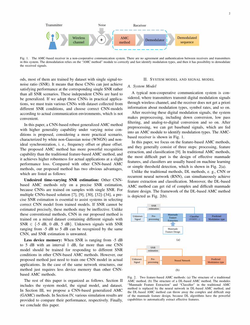
Fig. 1. The AMC-based receiver in a non-cooperative communication system. There are no agreement and authentication between receivers and transmittersin this system. The demodulation relies on the “AMC method” module to correctly and fast identify modulation types, and then it has possibility to demodulatethe received signals.

ods, most of them are trained by dataset with single signal-to-noise ratio (SNR). It means that these CNNs can just achievesatisfying performance at the corresponding single SNR ratherthan all SNR scenarios. These independent CNNs are hard tobe generalized. If we adopt these CNNs in practical applica-tions, we must train various CNNs with dataset collected fromdifferent SNR conditions, and choose correct CNN-modelsaccording to actual communication environments, which is notconvenient.

In this paper, a CNN-based robust generalized AMC methodwith higher generality capability under varying noise con-ditions is proposed, considering a more practical scenario,characterized by white non-Gaussian noise (WNGN) and non-ideal synchronization, i. e., frequency offset or phase offset.The proposed AMC method has more powerful recognitioncapability than the traditional feature-based AMC method, andit achieves higher robustness for actual applications at a slightperformance loss. Compared with other CNN-based AMCmethods, our proposed method has two obvious advantages,which are listed as follows:

Undesired time-varying SNR estimation: Other CNN-based AMC methods rely on a precise SNR estimation,because CNNs are trained on samples with single SNR. Formultiple CNNs-based solution [7], [9], [30], [32]–[34], a pre-cise SNR estimation is essential to assist systems in selectingcorrect CNN model from trained models. If SNR cannot beestimated precisely, these methods may be ineffective. Unlikethese conventional methods, CNN in our proposed method istrained on a mixed dataset containing different signals withSNR ∈ {-5 dB, 0 dB, 5 dB}. Unknown signals with SNRranging from -5 dB to 5 dB can be recognized by the sameCNN, and SNR estimation is unwanted.

Less device memory: When SNR is ranging from -5 dBto 5 dB with an interval 1 dB, far more than one CNNmodel should be trained for responding to different SNRconditions in other CNN-based AMC methods. However, ourproposed method just need to train one CNN model in actualapplications. In the case of the same network structures, ourmethod just requires less device memory than other CNN-based AMC methods.

The rest of this paper is organized as follows. Section IIincludes the system model, the signal model, and dataset.In Section III, we propose a CNN-based generalized AMC(GAMC) methods. In Section IV, various simulation results areprovided to compare their performance, respectively. Finally,we conclude this paper.

II. SYSTEM MODEL AND SIGNAL MODEL

A. System Model

A typical non-cooperative communication system is con-sidered, where transmitters transmit digital modulation signalsthrough wireless channel, and the receiver does not get a prioriinformation about modulation types, symbol rates, and so on.

After receiving these digital modulation signals, the systemmakes preprocessing, including down conversion, low passfiltering, and analog-to-digital conversion and so on. Afterpreprocessing, we can get baseband signals, which are fedinto an AMC module to identify modulation types. The AMC-based receiver is shown in Fig. 1.

In this paper, we focus on the feature-based AMC methods,and they generally consist of three steps: processing, featureextraction, and classification [9]. In traditional AMC methods,the most difficult part is the design of effective manmadefeatures, and classifiers are usually based on machine learningor simple threshold detection, which is shown in Fig. 2(a).

Unlike the traditional methods, DL methods, e. g., CNN orrecurrent neural network (RNN), can simultaneously achievefeature extraction and classification. Moreover, the DL-basedAMC method can get rid of complex and difficult manmadefeature design. The framework of the DL-based AMC methodis depicted as Fig. 2(b).

Manmade

Feature

Extraction

Classifier(SVM/DT/…)

Unknown

Signal

SNR

estimation

Predicted

Modulation type

Pre-

processing

Manmade

Feature Design

(a)

Unknown

Signal

SNR

estimation

Predicted

Modulation type

Pre-

processingNeural Network

(b)

Fig. 2. Two feature-based AMC methods: (a) The structure of a traditionalAMC method. (b) The structure of a DL-based AMC method. The modules“Manmade Feature Extraction” and “Classifier” in the traditional AMCmethod is replaced by the neural network in DL-based AMC method, andthe DL-based AMC method can throw away the complex and difficult stepof the manmade feature design, because DL algorithms have the powerfulcapabilities to automatically extract effective features.

3

B. Signal Model

Assuming that the received complex-valued baseband equiv-alent signal r(n) is sampled at the Nyquist rate, it is given asfollows.

r(n) = αej(∆θ+2π∆f nN )x(n) + w(n), n = 1, 2, ..., N, (1)

where α, ∆θ, ∆f , and N represent attenuation factor, carrierphase offset (CPO) caused by wireless channels [7], normal-ized carrier frequency offset (CFO), and the number of sam-pling points in an independent observation phase, respectively.In this paper, we consider a flat fading and time invariantchannel, so α, ∆θ, and ∆f are constant in each observationphase.

In addition, {x(n)}Nn=1 is the symbol sequence, and threemodulation types of frequency shift keying (FSK), phase shiftkeying (PSK), and quadrature amplitude modulation (QAM)are considered in this paper; w(n) represents additive noise.In this paper, we mainly consider WNGN based on Gaussianmixture model (GMM) with K components [35]. GMM-basedWNGN consists of K independent noise obeying complexGaussian distributions. Its probability density function (PDF)is given as

f(w(n)) =

K∑k=1

λk√πσ2

k

e−|w(n)|2

σ2k , (2)

and it consists of K independent noise obeying complexGaussian distributions. λk is the ratio of each component, and∑Kk=1 λk = 1 and 0 < λk < 1.In this paper, we consider a classical GMM-based WNGN

with two components of w0(n) and w1(n), and w(n) =λ0w0(n) + λ1w1(n). w0(n) is just additive white Gaussiannoise (AWGN), i. e., w1(n) ∼ CN(0, σ2

0). w1(n) is impulsivenoise with zero mean and the variance of σ2

1 , where σ1 � σ0

[36].

III. AMC METHODS

In this section, a CNN-based generalized AMC (GAMC)method is proposed with better generalization performanceunder varying noise conditions. In contrast, previous proposedCNN-based AMC method [7], [9], [30], [32]–[34] is denotedas a fixed AMC (FAMC) method, and it does not equip withpowerful generalization capability. In addition, traditional AM-C methods, based on classical manmade features and typicalmachine learning-based classifiers, are firstly introduced as acomparison.

A. Traditional AMC Method

For the purpose of highlighting the performance of DL-based AMC method, we adopt one of a traditional AMCmethod as a comparison. The structure of the traditional AMCmethod is shown in Fig. 2(a), where high-order cumulants(HOC) [37] are classical manmade features, which are de-scribed below.

In detail, the normalized fourth-order cumulants [38] areapplied, and they can be describe as:

C̃40 = M̃40 − 3M̃220, (3)

C̃41 = M̃41 − 3M̃21M̃20, (4)

C̃42 = M̃42 −∣∣∣M̃20

∣∣∣2 − 2M̃221, (5)

where M̃mk represents the normalized moments. It can bedenoted as M̃mk =

∑Nn=1 r

m−k(n)r∗k(n)

(∑Nn=1 |r(n)|2)m/2

, and r∗ (n) is theconjugate of r (n).

Hence,{C̃40, C̃41, C̃42

}works as a feature vector and SVM

acts as a clssifier.

B. CNN-based GAMC Method

Here, a CNN-based GAMC method is stated from dataset,CNN structure, classifier, loss function, and training and teststrategies.

1) Dataset: Dataset, applied in this paper, contains multiplein-phase and quadrature (IQ) samples, which is transformedfrom the received complex signal sequence. The receivedsequence is defined as R = {r(n)}Nn=1. To avoid the scalingproblem, the power of R should be normalized, and thenormalized received sequence R̃ is equal to R∑N

n=1 |r(n)|2 .

Then, we separate real part real(R̃)

and imaginary part

imag(R̃)

from the normalized received sequence. Next,

real(R̃)

and imag(R̃)

are combined into a matrix withdimension 2×N , which is treated as one sample for trainingor testing.

In addition, the real part and imaginary part are also in-phase (I) component and quadrature (Q) component of signal,respectively. So this training or test sample is also called asIQ sample, which is shown in eq. (6).

IQ =

[real(R̃)

imag(R̃)

]. (6)

2) CNN structure: The CNN consists of four main part-s: “Input”, “Output”, “Convolutional layer”, and “Fully-connected layer”, and its structure is depicted in Fig. 3.

Firstly, “Input” is the dataset with IQ samples and theircorresponding labels. Then, “Convolutional Layer” is to auto-matically extract features and contains two “Conv2D” layers.In these “Conv2D” layers, the convolutional kernel sizes are2× 4 and 1× 8, respectively, which are is designed accordingto input data: IQ sample, the dimensionality of which is 2×N .

Next, “Fully-connected Layer” is fundamentally a classifierwith three “Dense” layers, and its output is a probabilitydistribution, which contains the possibility of each modulationtype. Finally, “Output” is the predicted modulation type, and itis given by the maximum a posteriori (MAP) classifier basedon probability distribution of the last “Dense” layer.

Besides, rectified linear unit (ReLU) plays the role of theactivation function in each layer except the last dense layer,where Softmax is applied. Assuming that xi is the output of

4

Dataset

(IQ sam

ple, M

od

ulatio

n ty

pe)

Co

nv2

D (1

28

, 1×

8)

ReL

U+

BN

+D

rop

ou

t(0.5

)

Co

v2D

(64

, 2×

4)

ReL

U+

BN

+D

rop

ou

t(0

.5)

ReL

U+

BN

+D

rop

ou

t(0.5

)

Den

se (25

6)

Den

se (12

8)

ReL

U+

BN

+D

ropou

t(0

.5)

Den

se (3)

So

ftmax

Convolutional

LayerFully-connected

Layer

Pred

icted

mo

du

lation

typ

e

Input

Output

MA

P classifier

Fig. 3. The CNN structure with four parts: 1) Input: IQ samples and corresponding modulation types as labels; 2) Convolutional Layer: two Conv2Dlayers for feature extraction; 3) Fully-connected Layer: three Dense layers to give predicted probability distribution; 4) Output: a MAP classifier to classifymodulation types according to the predicted probability distribution.

the i-th neuron in a certain layer, the function of ReLU andSoftmax can be described as follows.

fReLU (xi) = max (0, xi) , fSoftmax (xi) =exi∑j exj. (7)

In addition, batch normalization (BN) and dropout, aftereach activation function (except in the last fully-connectedlayer), are applied to accelerate training, improve performanceslightly and avoid overfitting. They can be considered as twoimplicit regularization terms. BN is to normalize the output ofeach layer in each batch and can be represented as

BN(Oi) = γ · Oi −Mean(Ominibacth)√V ar(Ominibacth) + ε

+ β, (8)

where Mean(Ominibacth) and V ar(Ominibacth) are the meanand variance of the output of mini-batch data, respectively;γ and β are trainable parameters [39], and ε is a minimumvalue to prevent denominators from being zero. In addition,Dropout is to temporarily disable partial neurons with a certainprobability in the training process.

It is noted that the same CNN structure is applied into bothFAMC and GAMC.

3) MAP classifier: AMC is to identify modulation types ina limited modulation type candidate pool. Assuming that themodulation type candidate pool is M = {mi}

Ntypei=1 , where mi

represents a certain modulation type and this pool containsNtype different modulation types, MAP criterion in CNN-based AMC [36] can be described as:

m̂i = arg maxmi∈M

p(mi, fmodel,Θ|IQ), (9)

where m̂i is the predicted modulation type; fmodel representsmodel structure, and Θ = {Θtrainable,Θuntrainable} is themodel parameters, which contains massive trainable parame-ters and a few untrainable parameters; p(·) is a PDF that refersto the output of Softmax function in the last fully-connectedlayer.

4) Loss function: In this paper, the categorical cross entropy(CCE) function is applied as data loss function (or experienceloss function), considering that AMC is essentially a multi-class classification task.

Suppose the dataset T = {(si, li)}Nsi=1 is applied for thetraining of CNN, where si, li and Ns represents IQ sample,ground truth sample label through one-hot encoding, andthe number of training samples, respectively. The CCE lossfunction is given as follows.

LCCE(T ; fmodel,Θ) = −Ns∑i=1

lilog(fmodel (si; Θ)). (10)

However, the final loss function contains not only the dataloss function but also the structure loss function, and it can bewritten as follows.

L(T ; fmodel,Θ) =1

NsLCCE(T ; fmodel,Θ)

+ λmodelJ(fmodel,Θ),(11)

where J(·) is just the structure loss function (or regularizationterm), which is to avoid overfitting, and λmodel is appliedto balance these two loss functions. In this paper, BN anddropout are as the components of the structure loss function,which have been introduced above.

5) Training and test strategies: Training optimizer, trainingprocess, and test process are introduced in this part. Thesame training optimizer is adopted in both GAMC and FAMCmethod, and their main difference focuses on the training andtest process between our proposed GAMC method and FAMCmethod.

Training optimizer: stochastic gradient descent (SGD) isintroduced as an optimizer to minimize the function (11)by iteratively optimizing and updating trainable parametersΘtrainable in Θ. The optimizing rule is written as follows.

Θnewtrainable =Θnow

trainable

− η ∂L(T ; fmodel,Θnowtrainable,Θuntrainable)

∂Θnowtrainbale

,

(12)

where η is referred to as a learning rate to control scale ofparameter adjustment.

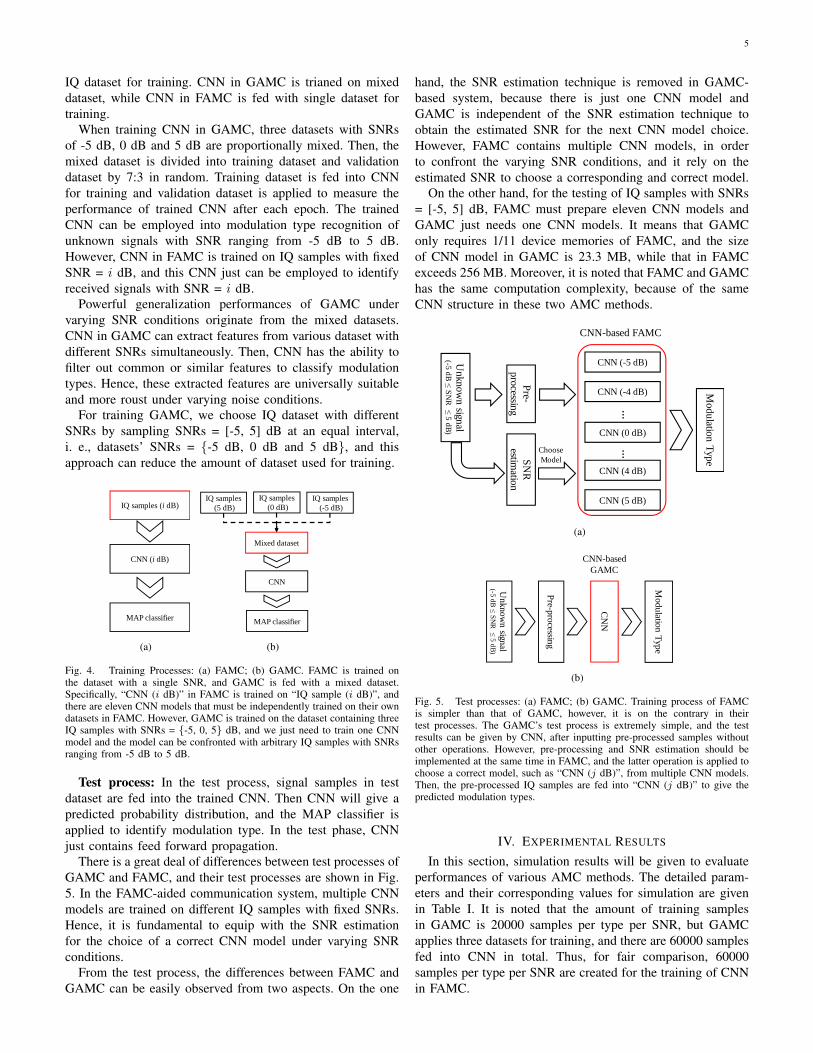
Training process: The training processes of GAMC andFAMC are shown in Fig. 4. From Fig. 4(a) and Fig. 4(b),it can be observed that GAMC differs from FAMC in the

5

IQ dataset for training. CNN in GAMC is trianed on mixeddataset, while CNN in FAMC is fed with single dataset fortraining.

When training CNN in GAMC, three datasets with SNRsof -5 dB, 0 dB and 5 dB are proportionally mixed. Then, themixed dataset is divided into training dataset and validationdataset by 7:3 in random. Training dataset is fed into CNNfor training and validation dataset is applied to measure theperformance of trained CNN after each epoch. The trainedCNN can be employed into modulation type recognition ofunknown signals with SNR ranging from -5 dB to 5 dB.However, CNN in FAMC is trained on IQ samples with fixedSNR = i dB, and this CNN just can be employed to identifyreceived signals with SNR = i dB.

Powerful generalization performances of GAMC undervarying SNR conditions originate from the mixed datasets.CNN in GAMC can extract features from various dataset withdifferent SNRs simultaneously. Then, CNN has the ability tofilter out common or similar features to classify modulationtypes. Hence, these extracted features are universally suitableand more roust under varying noise conditions.

For training GAMC, we choose IQ dataset with differentSNRs by sampling SNRs = [-5, 5] dB at an equal interval,i. e., datasets’ SNRs = {-5 dB, 0 dB and 5 dB}, and thisapproach can reduce the amount of dataset used for training.

CNN (i dB)

IQ samples (i dB)

MAP classifier

(a)

CNN

IQ samples

(5 dB)

MAP classifier

IQ samples

(0 dB)

IQ samples

(-5 dB)

Mixed dataset

(b)

Fig. 4. Training Processes: (a) FAMC; (b) GAMC. FAMC is trained onthe dataset with a single SNR, and GAMC is fed with a mixed dataset.Specifically, “CNN (i dB)” in FAMC is trained on “IQ sample (i dB)”, andthere are eleven CNN models that must be independently trained on their owndatasets in FAMC. However, GAMC is trained on the dataset containing threeIQ samples with SNRs = {-5, 0, 5} dB, and we just need to train one CNNmodel and the model can be confronted with arbitrary IQ samples with SNRsranging from -5 dB to 5 dB.

Test process: In the test process, signal samples in testdataset are fed into the trained CNN. Then CNN will give apredicted probability distribution, and the MAP classifier isapplied to identify modulation type. In the test phase, CNNjust contains feed forward propagation.

There is a great deal of differences between test processes ofGAMC and FAMC, and their test processes are shown in Fig.5. In the FAMC-aided communication system, multiple CNNmodels are trained on different IQ samples with fixed SNRs.Hence, it is fundamental to equip with the SNR estimationfor the choice of a correct CNN model under varying SNRconditions.

From the test process, the differences between FAMC andGAMC can be easily observed from two aspects. On the one

hand, the SNR estimation technique is removed in GAMC-based system, because there is just one CNN model andGAMC is independent of the SNR estimation technique toobtain the estimated SNR for the next CNN model choice.However, FAMC contains multiple CNN models, in orderto confront the varying SNR conditions, and it rely on theestimated SNR to choose a corresponding and correct model.

On the other hand, for the testing of IQ samples with SNRs= [-5, 5] dB, FAMC must prepare eleven CNN models andGAMC just needs one CNN models. It means that GAMConly requires 1/11 device memories of FAMC, and the sizeof CNN model in GAMC is 23.3 MB, while that in FAMCexceeds 256 MB. Moreover, it is noted that FAMC and GAMChas the same computation complexity, because of the sameCNN structure in these two AMC methods.

SN

R

estimatio

n

Modulatio

n T

ype

Pre-

pro

cessing

CNN (-5 dB)

CNN (0 dB)

CNN (5 dB)

……

CNN (4 dB)

CNN (-4 dB)

Un

kn

ow

n sig

nal

(-5 d

B≤

SN

R≤

5 d

B)

Choose

Model

CNN-based FAMC

(a)

CN

N

Un

kn

ow

n sig

nal

(-5 d

B≤

SN

R≤

5 d

B)

Pre-p

rocessin

g

Modulatio

n T

ype

CNN-based

GAMC

(b)

Fig. 5. Test processes: (a) FAMC; (b) GAMC. Training process of FAMCis simpler than that of GAMC, however, it is on the contrary in theirtest processes. The GAMC’s test process is extremely simple, and the testresults can be given by CNN, after inputting pre-processed samples withoutother operations. However, pre-processing and SNR estimation should beimplemented at the same time in FAMC, and the latter operation is applied tochoose a correct model, such as “CNN (j dB)”, from multiple CNN models.Then, the pre-processed IQ samples are fed into “CNN (j dB)” to give thepredicted modulation types.

IV. EXPERIMENTAL RESULTS

In this section, simulation results will be given to evaluateperformances of various AMC methods. The detailed param-eters and their corresponding values for simulation are givenin Table I. It is noted that the amount of training samplesin GAMC is 20000 samples per type per SNR, but GAMCapplies three datasets for training, and there are 60000 samplesfed into CNN in total. Thus, for fair comparison, 60000samples per type per SNR are created for the training of CNNin FAMC.

6

TABLE IEXPERIMENT PARAMETERS

Parameter ValueModulation type M={FSK, PSK, QAM},candidate pool Ntype = 3

WNGN λ0 = 0.9, λ1 = 0.1,(λ0, λ1, σ0, σ1) σ2

1/σ20 = 100

CPO ∆θ ∆θ ∼ U(0, φ], φ ∈{

2iπ16

}4

i=0

CFO ∆f ∆f ∈ {0.1 + 0.2i}4i=0The number of sampling N = 128

points NThe number of training 20000 samples/type/SNR

samples for GAMC (SNRs = {-5, 0, 5} dB)The number of training 60000 samples/type/SNR

samples for FAMC (SNRs = [-5, 5] dB)The number of test 30000 samples/type/SNR

samples Ntest (SNRs = [-5, 5] dB and NSNR = 11)Maximum training epochs 200

Batch sizes 500Learning rate η η = 0.001

TABLE IICOMPUTATION TIME OF FAMC, GAMC, AND TRADITIONAL AMC.

MethodTime (µs/sample) SNR (dB)

-5 0 5

FAMC/GAMC (GPU) 37.71FAMC/GAMC (CPU) 698.20

Traditional AMC (CPU) 2346.60 2225.19 1807.83* Considering that FAMC and GAMC have the same CNN structure, and

if ignoring calculation error, they have the same degree of computationcomplex, i. e., the same unit computation time.

The simulation requires powerful computing resources, soit is conducted on the platform with one Intel i7-8750H CPUand one NVIDIA GTX 1080Ti GPU. The implementation ofneural networks relies on Keras 2.2.2 with Tensorflow 1.10 andPython 3.6.5 as the backend. SVM is carried out in Sklearn-Python library. Moreover, Matlab R2018a is applied to buildour datasets.

Here, three metrics are applied to evaluate classificationperformances, and The former two metrics are correct clas-sification probability (CCP) at SNR= i dB: P icc and averagecorrect classification probability (AveCCP): Pcc, which areshown as follows.

P icc =N icc

Ntest ×Ntype× 100%, i ∈ {−5,−4, ..., 4, 5} , (13)

Pcc =

∑5i=−5N

icc

Ntest ×Ntype ×NSNR× 100%, (14)

where N icc, Ntest, and NSNR represent the number of cor-

rectly recognized samples at SNR= i dB, the amount of testsamples at each type and SNR, and the amount of samplingSNRs, respectively. P icc appears with the format of graphs andPcc is shown as table format.

For the visualization of the specific classification perfor-mance for each modulation type in various AMC methods,the third metric, applied in this paper, is the confusion matrixwith dimension 3× 3.

Fig. 6. The classification performance of FAMC, GAMC, and traditionalAMC with the condition of CFO and CPO. It can be observed that FAMCand GAMC have perfect and similar CCP at each SNR, and the classificationaccuracy of FAMC is slightly higher than that of GAMC, but traditional AMChas far weaker performance than these two CNN-based AMC methods.

(a) (b)

(c) (d)

(e) (f)

Fig. 7. Confusion matrices of FAMC and GAMC without the considerationof CFO and CPO. FAMC: (a) -5 dB; (b) 0 dB; (c) 5 dB. GAMC: (d) -5 dB;(e) 0 dB; (f) 5 dB.

A. Classification performance and computation complexity ofFAMC, GAMC and traditional AMC

The specifies of various AMC methods under WNGN con-dition and without CFO and CPO are depicted in Fig. 6. Fromthese experimental results, we can observe that the traditional

7

(a)

(b)

Fig. 9. The classification performance of GAMC considering different CFOs and CPOs. With the increase of the normalized CFO, the classificationperformance of GAMC is slightly affected. However, the increasing CPO leads to the sharp performance degradation, while it has the limited performancedecline at high SNR, such as 5 dB.

Fig. 8. The specific classification performance of FAMC and GAMC withthe considering of CFO (∆f = 0.9) and CPO (φ = π), respectively. FAMCand GAMC with the consideration of CPO have lower P icc than that withoutthe consideration of CPO or with the consideration of CFO. In addition, thereis the limited performance gap between FAMC and its corresponding GAMC.

TABLE IIITHE AVERAGE CORRECT CLASSIFICATION PROBABILITY OF DIFFERENT

AMC METHODS.

Methods Pcc (%)FAMC (Benchmark) 86.55

GAMC 85.79Traditonal AMC 42.85

FAMC (∆f = 0.9, φ = 0) 85.69GAMC (∆f = 0.9, φ = 0) 84.86FAMC (∆f = 0, φ = π) 82.14GAMC (∆f = 0, φ = π) 81.13

AMC method, based on SVM and HOC, has unsatisfactoryperformances, compared with the CNN-based AMC methods.P icc of GAMC is similar with that of FAMC, and their

maximum gap of P icc only can reach up to 1.22% at SNR= 2 dB or -5 dB. It means that GAMC and FAMC has fewperformance gap. In addition, this phenomenon also appearsin the other metric: Pcc, and their performance gap of Pcc isless than 1%, which is shown in Table III.

The confusion matrices of FAMC and GAMC at three SNRsare given in Fig. 7. Compared with the confusion matrices

(a) (b)

(c) (d)

(e) (f)

Fig. 10. Confusion matrices of FAMC and GAMC with the considerationof CFO and ∆f = 0.9. The confusion matrices of FAMC at SNRs = -5, 0, 5dB are given in (a), (b), and (c). Corresponding confusion matrices of GAMCare shown in (d), (e), and (f).

of FAMC and GAMC at the same SNR, they are extremelysimilar. At low SNR, both FAMC and GAMC can barelyidentify PSK and QAM, but their classification performancesare gradually improved, as SNR increases. However, FSK

8

(a) (b)

(c) (d)

(e) (f)

Fig. 11. Confusion matrices of FAMC and GAMC with the considerationof CPO and φ = π. (a) FAMC at SNR = -5 dB; (b) FAMC at SNR = 0 dB;(c) FAMC at SNR = 5 dB; (d) GAMC at SNR = -5 dB; (e) GAMC at SNR= 0 dB; (f) GAMC at SNR = 5 dB.

can be precisely distinguished from other modulation typesin these two AMC methods, even at low SNR, such as -5 dB.

Besides, computation cost or computation complex is an-other metric to measure AMC methods. In this paper, unitcomputation time is applied as a metric for the evaluationof three methods, which are shown in Table II. The timerepresents the average computation time of single IQ sampleafter testing a large number of samples, and it is calculated inthe same platform listed in the head of this section.

From Table II, it can be observed that FAMC and GAMCnot only on GPU but also on CPU have far higher compu-tation speed than traditional AMC. These results demonstratethat the CNN-based AMC methods are more efficient thanthe traditional AMC, particularly in communication systemsequipped with GPU.

B. Classification performance of FAMC and GAMC consider-ing CFO and CPO

In this section, the traditional AMC is not considered,because of the weak classification performance and slowcomputation speed. The influence of CFO and CPO for theclassification performances of the CNN-based AMC methodis shown in Fig. 8 and Table III. It is noted that the normalized

TABLE IVTHE AVERAGE CORRECT

CLASSIFICATION PROBABILITYOF GAMC CONSIDERING

DIFFERENT CFOS.

∆f Pcc (%)0 85.79

0.1 85.830.3 85.210.5 85.080.7 84.890.9 84.86

TABLE VTHE AVERAGE CORRECT

CLASSIFICATION PROBABILITYOF GAMC CONSIDERING

DIFFERENT CPOS.

φ Pcc (%)0 85.79

π/16 85.45π/8 83.99π/4 82.64π/2 82.10π 81.13

CFO has few effect on FAMC and GAMC, while theiridentification capabilities are both worse under the influenceof CPO.

What’s more there are almost no expansion of the classifi-cation performance gap between FAMC and GAMC, becausetheir Pcc gap of FAMC and GAMC are within or slightlyhigher than 1%. In addition, their maximum P icc gap is 1.01%with the consideration of CFO, while the value just reaches upto 1.49%, when considering CPO. The confusion matrices inFig. 10 and Fig. 11 also illustrates that FAMC and GAMC havesimilar performances under any circumstances in this paper.

Then, the classification performances of GAMC under thecondition of different CFOs and CPOs is considered, and theirexperimental results are shown in Fig. 9, Table IV and TableV. As mentioned before, P icc and Pcc of GAMC is almostunaffected by normalized CFO.

As is shown in Fig. 9(b) and Table V, the influence of CPOis weak at φ = π

16 or high SNR, such as 5 dB. However,the influence of CPO is gradually getting strong with theincrease of the value of φ. Phase offset correction algorithmsshould be considered to aid CNN-based AMC methods forthe improvement of classification performances, when φ is toolarge.

C. Generalization capabilities under varying SNR conditions

In the former sections, the specific classification perfor-mances of FAMC and GAMC have been introduced carefullythrough three metrics, and it can be concluded that thereare extremely weak performance gaps between FAMC andGAMC. In this section, it is illustrated that GAMC has morepowerful generalization capabilities than FAMC at the expenseof the slight performance loss. What’s more, we give two setsof simulation results for generalization capabilities. The oneset of results is tested within the ranges of training SNRs, i.e., SNRs = [-5, 5] dB, and the other set is out of the ranges,including SNRs = [-15, -6] dB and [6, 15] dB.

1) Within the range of training SNRs: To compare thegeneralization capabilities between FAMC and GAMC undervarying noise conditions, we depict three curves of CNN (jdB) in FAMC trained at different SNRs (i. e., j = -5, 0, 5) inFig. 12, and we tested them at SNRs ranging from -5 dB to5 dB.

The CNN (j dB) in FAMC performs well when testingSNRs are close to j dB (1 dB error can be allowed), butits performance gets worse at other SNRs, which means thatthe FAMC does not have higher robustness and generalization

9

(a)

(b)

(c)

Fig. 12. Generalization capability of FAMC and GAMC. (a) is just underWNGN condition without the consideration of CFO and CPO; (b) and (C)are under WNGN condition considering CFO and CPO, respectively.

capabilities. On the contrary, Fig. 12 demonstrates that GAMCcan work well at all the testing SNRs, whether or not CFOand CPO are considered.

2) Out of the scope of training SNRs: In order to make thefuture compare the generalization capabilities of FAMC andGAMC, we present the simulation results for SNRs outsidethe range of training SNRs in Fig. 13. In Fig. 13(a), the CCPsof GAMC at SNRs, which is higher than 5 dB, is far beyondthat of FAMC. The similar simulation results also appear inFig. 13(b), when SNR is lower than -5 dB.

It is demonstrated that GAMC can extract more robustfeatures from the mixed datasets than FAMC, and GAMChas more powerful generalization capabilities than FAMC. Inaddition, we only prepare eleven trained CNN models, i. e.,CNN (i dB) and i ∈ {−5,−4, ..., 4, 5}. So we have to applyCNN (−5 dB) or CNN (5 dB) into noise conditions with SNRs= [-15, -6] dB or [6, 15] dB.

(a)

(b)

Fig. 13. Generalization capabilities of FAMC and GAMC out of the rangeof training SNRs.

V. CONCLUSION

In this paper, we have proposed a CNN-based GAMCmethod with better robustness under varying noise conditions.Compared with the traditional AMC method, the classificationaccuracy of GAMC is far beyond. Besides, GAMC is morerobust than FAMC at the cost of negligible performance loss,because the CNN in GAMC is trained by a mixed IQ datasetcontaining received signals with SNRs of -5 dB, 0 dB and 5dB, and it can be applied to recognize modulation types ofsignals with uncertain SNR from -5 dB to 5 dB. Moreover,our proposed GAMC method is more practical than the CNN-based FAMC methods, because we just have to train oneCNN model in GAMC rather than many CNN models inFAMC, which means less device memory assumption. Inaddition, precise SNR estimation is unnecessary for GAMCto choose suitable CNN models. Hence, our proposed CNN-based GAMC method is meaningful for practical applications.

10

What’s more, the CNN in FAMC works perfectly, yet thisCNN can also be applied into GAMC with more complexmixed dataset. It is demonstrated by experimental results thatthe CNN in GAMC has the capability to extract universal androbust features from mixed dataset with different SNRs. It alsoillustrates that the CNN, designed by human experience here,has massive redundancy and its operation speed is also limited.Thus, our future work will focus on finding more effective andstreamlined neural network model, such as network slimmingalgorithm [40] and neural architecture search (NAS) [41].

REFERENCES

[1] H. Wu, M. Saquib, Z. Yun, “Novel Automatic Modulation ClassificationUsing Cumulant Features for Communications via Multipath Channels,”IEEE Transactions on Wireless Communications, vol. 7, no. 8, pp. 3098– 3105, Aug. 2008.

[2] L. Haring, Y. Chen, A. Czylwik, “Automatic Modulation ClassificationMethods for Wireless OFDM Systems in TDD Mode,” IEEE Transac-tions on Communications, vol. 58, no. 9, pp. 2480 – 2485, Sept. 2010.

[3] M. Aslam, Z. Zhu, A. Nandi, “Automatic Modulation ClassificationUsing Combination of Genetic Programming and KNN,” IEEE Trans-actions on Wireless Communications, vol. 11, no. 8, pp. 2742 – 2750,2012.

[4] S. Hakimi, and G. Abed Hodtani, “Optimized Distributed AutomaticModulation Classification in Wireless Sensor Networks Using Informa-tion Theoretic Measures,” IEEE Sensors Journal, vol. 17, no. 10, pp.3079 – 3091, Oct. 2017.

[5] Z. Zhu, A. Nandi, Automatic Modulation Classification: Principles,Algorithms and Applications, John Wiley & Sons, 2015.

[6] S. Rajendran, W. Meert, D. Giustiniano, V. Lenders, S. Pollin, “DeepLearning Models for Wireless Signal Classification With DistributedLow-Cost Spectrum Sensors,” IEEE Transactions on Cognitive Com-munications and Networking, vol. 4, no. 3, pp. 433-445, Mar. 2018.

[7] F. Meng, P. Chen, L. Wu, and X. Wang, “Automatic ModulationClassification: A Deep Learning Enabled Approach,” IEEE Transactionson Vehicular Technology, vol. 67, no. 11, pp. 10760 – 10772, 2018.

[8] F. Hameed, O. A. Dobre, D. C. Popescu, “On the Likelihood-basedApproach to Modulation Classification,” IEEE Transactions on WirelessCommunications, vol. 8, no. 12, pp. 5884-5892, 2009.

[9] Z. Yin, et al., “Robust Automatic Modulation Classification UnderVarying Noise Conditions,” IEEE Access, vol. 5, no. 1, pp. 19733 –19741, 2017.

[10] Z. Fadlullah, et al., ”State-of-the-Art Deep Learning: Evolving MachineIntelligence Toward Tomorrow’s Intelligent Network Traffic ControlSystems,” IEEE Communications Surveys & Tutorials, vol. 19, no. 4,pp. 2432 – 2455, 2017.

[11] Y. Zhou, Z. Fadlullah, B. Mao, N. Kato, “A Deep-Learning-Based RadioResource Assignment Technique for 5G Ultra Dense Networks,” IEEENetwork, vol. 32, no. 6, pp. 28-34, Dec. 2018.

[12] B. Mao, et al., “A Novel Non-Supervised Deep Learning Based NetworkTraffic Control Method for Software Defined Wireless Networks,” IEEEWireless Communications Magazine, vol. 25, no. 4, pp. 74 – 81, 2018.

[13] C. K. Wen, W. T. Shih, and S. Jin, “Deep Learning for Massive MIMOCSI Feedback,” IEEE Wireless Communications Letters, vol. 7, no. 5,pp. 748–751, 2018.

[14] J. Wang, et al., “Device-Free Wireless Localization and Activity Recog-nition: A Deep Learning Approach,” IEEE Transactions on VehicularTechnology, vol. 66, no. 7, pp. 44 – 55, Jul. 2017.

[15] Y. Xing, et al., “Driver Activity Recognition for Intelligent Vehicles: ADeep Learning Approach,” IEEE Transactions on Vehicular Technology,to be published, doi: 10.1109/TVT.2019.2908425

[16] P. Zhou, et al., “Deep Learning-Based Beam Management and Interfer-ence Coordination in Dense mmWave Networks,” IEEE Transactions onVehicular Technology, vol. 68, no. 1, pp. 592 – 603, Jan. 2019.

[17] H. Jiang, et al., “A 3D Non-Stationary Wideband Geometry-BasedChannel Model for MIMO Vehicle-to-Vehicle Communication Systems,”IEEE Transactions on Vehicular Technology, to be published, 2019.

[18] X. Sun, et al., “ResInNet: A Novel Deep Neural Network with FeatureReuse for Internet of Things,” IEEE Internet Things Journal, vol. 6, no.1, pp. 679 – 691, 2018.

[19] H. Huang, Y. Song, and J. Yang, “Deep-Learning-based Millimeter-WaveMassive MIMO for Hybrid Precoding,” IEEE Transactions on VehicularTechnology, vol. 68, no. 3, pp. 3027 – 3032, 2019.

[20] H. Huang, et al., “Deep Learning for Super-Resolution Channel Es-timation and DOA Estimation based Massive MIMO System,” IEEETransactions on Vehicular Technology, vol. 67, no. 9, pp. 8549 – 8560,2018.

[21] M. Liu, et al., “DSF-NOMA: UAV-Assisted Emergency CommunicationTechnology in a Heterogeneous Internet of Things,” IEEE InternetThings Journal, to be Publish doi 10.1109/JIOT.2019.2903165.

[22] F. Tang, Z. M. Fadlullah, B. Mao, and N. Kato, “An Intelligent TrafficLoad Prediction Based Adaptive Channel Assignment Algorithm inSDN-IoT: A Deep Learning Approach,” IEEE Internet Things Journal,vol. 5, no. 6, pp. 5141 – 5154, 2018.

[23] F. Tang, B. Mao, Z. Fadlullah, and N. Kato, “On a Novel Deep-Learning-Based Intelligent Partially Overlapping Channel Assignment in SDN-IoT,” IEEE Communications Magazine, vol. 56, no. 9, pp. 80 – 86,2018.

[24] W. Kang and D. Kim, “DeepRT: A Predictable Deep Learning InferenceFramework for IoT Devices,” IEEE/ACM Third International Conferenceon Internet-of-Things Design and Implementation (IoTDI), pp. 279 –280, 2018.

[25] H. Huang, et al., “Unsupervised Learning Based Fast BeamformingDesign for Downlink MIMO,” IEEE Access, vol. 7, no. 1, pp. 7599– 7605, 2019.

[26] H. Huang, et al., “Fast Beamforming Design via Deep Learning,”IEEE Transactions on Vehicular Technology, to be published, doi:10.1109/TVT.2019.2949122.

[27] G. Gui, H. Huang, Y. Song, and H. Sari, “Deep Learning for anEffective Nonorthogonal Multiple Access Scheme,” IEEE Transactionson Vehicular Technology, vol. 67, no. 9, pp. 8440 – 8450, 2018.

[28] M. Liu, T. Song, and G. Gui, “Deep Cognitive Perspective: ResourceAllocation for NOMA based Heterogeneous IoT with Imperfect SIC,”IEEE Internet Things Journal, vol. 6, no. 2, pp. 2885 – 2894, Feb. 2019.

[29] M. Liu, et al., “Deep Learning-Inspired Message Passing Algorithmfor Efficient Resource Allocation in Cognitive Radio Networks,” IEEETransactions on Vehicular Technology, vol. 68, no. 1, pp. 641 – 653,2018.

[30] T. O’Shea and J. Hoydis, “An Introduction to Deep Learning for thePhysical Layer,” IEEE Transactions on Cognitive Communications andNetworking, vol. 3, no. 4, pp. 563 – 575, 2017.

[31] B. Tang, Y. Tu, Z. Zhang, and Y. Lin, “Digital Signal ModulationClassification With Data Augmentation Using Generative AdversarialNets in Cognitive Radio Networks,” IEEE Access, vol. 6, pp. 15713 –15722, 2018.

[32] Y. Lin, Y. Tu, Z. Dou, and Z. Wu, “The Application of Deep Learningin Communication Signal Modulation Recognition,” in IEEE/CIC Inter-national Conference on Communications in China (ICCC), 2017, pp. 1– 5.

[33] Y. Tu and Y. Lin, “Deep Neural Network Compression Technique To-wards Efficient Digital Signal Modulation Recognition in Edge Device,”IEEE Access, vol. 7, pp. 58113 – 58119, 2019.

[34] Y. Wang, M. Liu, J. Yang, and G. Gui, “Data-Driven Deep Learningfor Automatic Modulation Recognition in Cognitive Radios,” IEEETransactions on Vehicular Technology, vol. 68, no. 4, pp. 4074 – 4077,2019.

[35] D. Middleton, “Non-Gaussian Noise Models in Signal Processing forTelecommunications: New Methods an Results for Class A and Class BNoise Models,” IEEE Transactions on Information Theory, vol. 45, no.4, pp. 1129 – 1149, 1999.

[36] S. Hu, et al., “Robust Modulation Classification under Uncertain NoiseCondition Using Recurrent Neural Network,” in IEEE Global Commu-nications Conference (GLOBECOM), 2018, pp. 1 – 7.

[37] A. Hazza, M. Shoaib, S. A. Alshebeili, and A. Fahad, “An Overviewof Feature-Based Methods for Digital Modulation Classification,” inInternational Conference on Communications, Signal Processing, andtheir Applications (ICCSPA), 2013, pp. 1 – 6.

[38] K. Hassan, I. Dayoub, W. Hamouda, et al.,“Blind Digital ModulationIdentification for Spatially-correlated MIMO Systems,” IEEE Transac-tions on Wireless Communications, vol. 11, no. 2, pp. 683 – 693, 2011.

[39] S. Ioffe, C. Szegedy, “Batch Normalization: Accelerating Deep Net-workTraining by Reducing Internal Covariate Shift” arXiv preprint,arXiv:1502.03167, 2015.

[40] Z. Liu, J. Li, Z. Shen, et al, “Learning Efficient Convolutional NetworksThrough Network Slimming,” in ICCV, Venice, Italy, Oct. 22–29, 2017,pp. 2736 – 2744.

[41] C. Liu, B. Zoph, M. Neumann, et al, “Progressive Neural ArchitectureSearch,” in European Conference on Computer Vision (ECCV), 2018,pp. 19 – 34.