generalized compensation principle

Generalized Compensation Principle

Aleh Tsyvinski1 Nicolas Werquin2

1Yale University

2Toulouse School of Economics

Becker Friedman Institute, May 2018

1 / 18

Introduction

• An economic disruption typically creates winners and losers

• e.g., technological change, immigration inflow, trade liberalization

• more generally, any shock that affects the wage distribution

• Welfare compensation problem:

• can we design a reform of the tax-and-transfer system . . .

• that offsets these losses by redistributing the gains of the winners . . .

• and if so, is it budget-feasible?

• Traditional PF [Kaldor 1939, Hicks 1939/40]: compensating variation

• amount that agent i is willing to pay to be as well off as before the shocks

• simple implementation if lump-sum taxes are available policy instruments

2 / 18

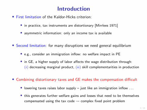
Introduction• First limitation of the Kaldor-Hicks criterion:

• in practice, tax instruments are distortionary [Mirrlees 1971]

• asymmetric information: only an income tax is available

• Second limitation: for many disruptions we need general equilibrium

• e.g., consider an immigration inflow: no welfare impact in PE

• in GE, a higher supply of labor affects the wage distribution through:

(i) decreasing marginal product, (ii) skill complementarities in production

• Combining distortionary taxes and GE makes the compensation difficult

• lowering taxes raises labor supply – just like an immigration inflow . . .

• this generates further welfare gains and losses that need to be themselves

compensated using the tax code complex fixed point problem

3 / 18

Introduction• Goal: design tax reform to bring each agent’s utility back to initial level

• consider (marginal) disruption of wage distribution in arbitrary direction

• main result: compensating tax reform and fiscal surplus in closed-form

• application: compensating the impact of automation (robots) in the US

• First step: partial equilibrium environment with distortionary taxes

• key: to a first order, indirect utility moves one-for-one with total tax bill

• because envelope theorem marginal tax rate does not affect welfare

• adjust average tax rate to cancel out the exogenous wage disruption

• GE: simultaneously solve for average and marginal tax rates (IDE)

• key: marginal tax rate directly affects welfare, even conditional on ATR

• because changes in labor supply (MTR) impact wages, and hence utility

• progressive reform at rate = ratio of labor demand vs. supply elasticities

4 / 18

Outline

1 The Welfare Compensation Problem

2 Design of the Compensating Tax Reform

3 Application: Compensating the Impact of Robots

5 / 18

Initial equilibrium

• Individuals i ∈ [0, 1]: wage wi, labor supply li, income tax T (wili)

welfare: Ui = maxli>0

ui (wili − T (wili) , li)

• Endogenous labor supply: first-order condition [FOC]

labor supply: li satisfies −u′i,l (ci, li)

u′i,c (ci, li)= [1− T ′ (wili)] wi

• Endogenous wage: marginal product of aggregate labor input [MPL]

wage: wi = F ′i (Ljj∈[0,1])

• Government tax revenue R given the tax schedule T

• in the paper: endogenous participation decisions, capital ownership

6 / 18

Wage disruptions and tax reforms

• Arbitrary disruption wE = wEi i∈[0,1] of the wage distribution w

• e.g, due to exogenous change F in the production function (tech change)

• before agent i adjusts behavior perturbed wage is wi (1 + µwEi )

• government implements tax reform T perturbed tax schedule T + µT

• New equil. (wi(1 + µwEi + µwi), li(1 + µli), Ui+µUi, T+µT )

• individuals adjust labor supply, which further impacts their wage, etc

• wii∈[0,1]: total endogenous (percentage) changes in wages formal

• Welfare compensation problem: find T s.t. Ui = 0 ∀i in new equil.

• focus on marginal disruptions in the direction wE : size µ→ 0

• once we solve for T , deriving the fiscal surplus R is straightforward

7 / 18

Outline




8 / 18

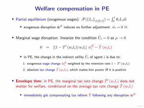
Welfare compensation in PE

• Partial equilibrium (exogenous wages): F (Lii∈[0,1]) =∫ 1

0θiLidi

• exogenous disruption wE induces no further adjustment: wi = 0 ∀i

• Marginal wage disruption: linearize the condition Ui = 0 as µ→ 0

0 = [(1− T ′ (wili))wili] wEi − T (wili)

• in PE, the change in the indirect utility Ui of agent i is due to:

1. exogenous wage change wEi weighted by the retention rate 1− T ′ (wili)

2. absolute tax change T (wili), which makes him poorer iff it is positive

• Envelope thm: in PE, the marginal tax rate change T ′ (wili) does not

matter for welfare, conditional on the average tax rate change T (wili)

• immediately get compensating tax reform T following any disruption wE

9 / 18

Elasticities

• Conclusion: compensating tax reform with distortionary taxes in PE

• adjust average tax rate by the net income gain or loss due to disruption

T (yi)

yi=

(1− T ′ (yi)

)wE

i

• GE: tax formulas in terms of standard (observable) elasticities formal

• labor supply elasticities of li wrt retention rate, wage: εS,ri , εS,wi [Hicks]

• labor supply elasticity of li wrt non-labor income: εS,ni [income effect]

• cross-wage elasticity of wj wrt Li: γji [skill complementarities in prod.]

γji discontinuous at j ≈ i

• own-wage elasticity of wi wrt Li:1

εDi[decreasing mg product of labor]

inverse elasticity of labor demand

10 / 18

Welfare compensation problem in GE

• GE: Linearizing the zero compensating variation condition Ui = 0

0 = [(1− T ′ (wili)) li] (wEi + wi)− T (wili)

• MPL: endogenous wage adjustment wi = − 1εDi

li +∫ 1

0γij ljdj

• FOC: total labor supply adjustment li = lpei + εS,wi

∫ 1

0Γij l

pej dj

elasticity Γij accounts for infinite series of cross-wage effects [Sachs Tsyvinski Werquin 17]

• where PE incidence: lpei = εS,wi wEi − εS,ri

T ′(yi)1−T ′(yi)

+ εS,niT (yi)

(1−T ′(yi))yi

• Key: In GE, changes in labor supply, and hence in MTR, have 1st-order

welfare effects despite the envelope theorem because they impact wages

• higher marginal tax rate raises utility: hours ↓ & wage ↑ [cf. Stiglitz 82]

11 / 18

Welfare compensation in GE: Solution• Compensating reform T solution to functional (integro-differential) eqn

• main result: solve for reform T (and fiscal surplus) in closed-form

• same formula with endogenous participation decisions and capital

• Proposition: The compensating tax reform is given in closed-form by

T (yi)

yi= (1− T ′ (yi))

[∫ 1

i

E ij ΩEj dj + Λi

]formal where: ΩE

j is the modified wage disruption variable

accounts for incidence of the initial shock wEi (labor demand spillovers in closed-form)

formal where: E ij is the progressivity variable

implies a progressive compensating reform. CES-CRP: E ij ∝ yεD/εS,r−p

i

formal where: Λi is the compensation-of-compensation variableseries Λi =

∑n Λ

(n)i of compensations. Λ constant with CES (uniform shift in tax rates)

12 / 18

Progressivity of the compensating tax reform

• E ij : assume decreasing MPL, infinite substitutability between skills

• in PE, the compensating tax reform is T (yi)yi

= (1− T ′ (yi)) wEi

• in GE, ATR must compensate both the wage disruption and the welfare

effects generated endogenously by the marginal tax rate changes

T (yi)

yi=

(1− T ′ (yi)

)ΩE

i +[1− p + (εD/εS,r)

]−1T ′ (yi)

• suppose agents i < i∗ are undisrupted progressive tax reform, because

in GE, an average tax hike must be compensated by a marginal tax hike

• Consequence [ODE]: ATR evolve below yi∗ at constant rate εD

εS,r − p > 0

T (yi)

yi∝ y

εD/εS,r−pi Iyi≤yi∗

• rate of progressivity: labor demand elasticity ÷ labor supply elasticity

• key: this ratio determines how much ↑ mg tax rate ↑ wage / utility

13 / 18

Graphical representation

• Calibration: constant elasticities (ε, σ, p) = (0.33 , 0.6 , 0.156)

compensation of a $100 gross income loss at yi∗ = $20K, $60K

0 20 40 60 80 100 120Income y in $1,000

-100

-90

-80

-70

-60

-50

-40

-30

-20

-10

0

y×w

E y/w

y

Wage Disruption at $20,000

Wage Disruption at $60,000

0 20 40 60 80 100 120Income in $1,000

-70

-60

-50

-40

-30

-20

-10

0

Tin

$

T PE(y)

TGE(y)

T PE(y)

TGE(y)

14 / 18

Outline




15 / 18

Automation in the U.S., 1990-2007

• Quantitative application based on Acemoglu and Restrepo (2017)

1990-2007: one additional robot per 1000 workers

1 2 3 4 5 6

Yearly income (1990) 104

-3

-2.5

-2

-1.5

-1

-0.5

0

0.5

1

1.5

Wag

e di

srup

tion

Wage disruption (% effect on wages 1990-2007)

Wage disruption95% confidence interval

0 1 2 3 4 5 6 7


-150

-100

-50

0

50

100

150

200

250

Inco

me

and

tax

chan

ges

($)

Income losses and partial-equilibrium compensation

Income gains and lossesTax bill change

16 / 18

Compensation in GE

• Compensating tax changes: −$113 at 10th centile (112% income loss),

+$260 at 90th percentile (124% income gain) fiscal surplus $16

0 1 2 3 4 5 6 7


-150

-100

-50

0

50

100

150

200

250

300

Tax

bill

cha

nge

($)

General-equilibrium compensation (U.S.)

0 1 2 3 4 5 6 7


-2.5

-2

-1.5

-1

-0.5

0

0.5

Ave

rage

tax

rate

cha

nge

(per

cent

age

poin

ts)

Compensation (U.S.): Average tax rates

17 / 18

Conclusion• Classic PF question: economic shock generally creates winners and losers

Kaldor 39, Hicks 39/40, Kaplow 04/12, Hendren 14

• design a compensating tax reform and evaluate its fiscal surplus

• closed-form tax reform in general equilibrium with only distortionary taxes

• more generally: compensate so that welfare of agent i changes by hi ∈ R

• Applications: automation, job polarization, immigration, intl trade

Acemoglu Restrepo 17, Goos et al 14, Dustmann Frattini Preston 13, Antras Gortari Itshkoki 17

• need GE framework: relative wages determined by relative supply of skills

• Advantages of compensation principle over optimal taxation

Stiglitz 82, Rothschild Scheuer 13/16, Ales Kurnaz Sleet 15, Sachs Tsyvinski Werquin 16

• policy-relevance: work with actual tax system and observable variables

• tractability (closed form) in much more general environments

• no need to choose a particular social welfare function

18 / 18

generalized compensation principle

Documents