The Volterra Principle Generalized

Tim Räz∗

September 16, 2016

Abstract

Michael Weisberg and Kenneth Reisman argue that the so-called Vol-terra Principle can be derived from a series of predator-prey models, andthat, therefore, the Volterra Principle is a prime example for the practiceof robustness analysis. In the present paper, I give new results regardingthe Volterra Principle, extending Weisberg’s and Reisman’s work, andI discuss the consequences of these new results for robustness analysis.I argue that we do not end up with multiple, independent models, butrather with one general model. I identify the kind of situation in whichthis generalization approach may occur, I analyze the generalized VolterraPrinciple from an explanatory perspective, and I propose that cases inwhich the generalization approach may not apply are in fact cases ofmathematical coincidences.

Contents1 Introduction 2

2 The Lotka-Volterra Predator-Prey Model 2

3 Robustness Analysis 4

4 The Volterra Principle Generalized 9

5 Weisberg’s Volterra Principle Revisited 13

6 Robustness Analysis and Generalization 14

7 The Generalized Volterra Principle as an Explanation 17

8 Robustness Analysis and Coincidence 18

9 Conclusion 20∗e-mail: tim.raez@gmail.com

1

A Models with Density Dependence and Predator Satiation 21

1 IntroductionThe Lotka-Volterra predator-prey model is historically important, because it ini-tiated mathematical modeling in biology. It is also philosophically important,because it is a much-discussed case study in the debates on scientific modeling,explanation, idealization, and robustness analysis. One of the most importantresults of the Lotka-Volterra predator-prey model is the Volterra Principle. Thisprinciple, first formulated as the “Third Law” by Vito Volterra, is supposed toexplain an empirical regularity about fishery statistics. However, the Lotka-Volterra predator-prey model is highly idealized, to the point that a realisticinterpretation of the model is questionable. Does this mean that the VolterraPrinciple is questionable as well? Michael Weisberg (2006b), and Michael Weis-berg and Kenneth Reisman (2008) argue that this is not the case. They proposethat the Volterra Principle can also be established from other predator-preymodels. According to Weisberg, the Volterra Principle is thus a prime examplefor the practice of robustness analysis.

In the present paper, I present new results concerning the Volterra Principle,extending and refining Weisberg’s and Reisman’s work, and I discuss the conse-quences of these new results for robustness analysis. The results are in keepingwith the goals of robustness analysis proposed by Weisberg. However, theydeviate from the process of robustness analysis that Weisberg proposes. In par-ticular, we do not end up with multiple independent models, but rather with onegeneral model. I identify the situations in which this generalization approachmay apply. I analyze the generalized Volterra Principle from an explanatoryperspective, and I show that my results exhibit several virtues of mathematicalexplanations. Finally, I discuss cases where the generalization approach may notapply, and I propose that these are in fact cases of mathematical coincidences.

2 The Lotka-Volterra Predator-Prey ModelThe Lotka-Volterra predator-prey model was originally proposed by Alfred Lotkaand Vito Volterra.1 Formally, the model is a set of two coupled ordinary dif-ferential equations. These equations are intended to capture the interactionsbetween a population of prey animals, and a population of predators, whichfeed on the prey.2 The model can be written as follows:

1See Knuuttila and Loettgers (2016) for a discussion of the contrast between Lotka’s andVolterra’s approach to scientific modeling in general, and to their eponymous model in par-ticular.

2Kot (2001) gives a detailed and accessible introduction to the mathematical aspects ofthe Lotka-Volterra model, and predator-prey models in general.

2

x = rx− axy (1)y = bxy −my (2)

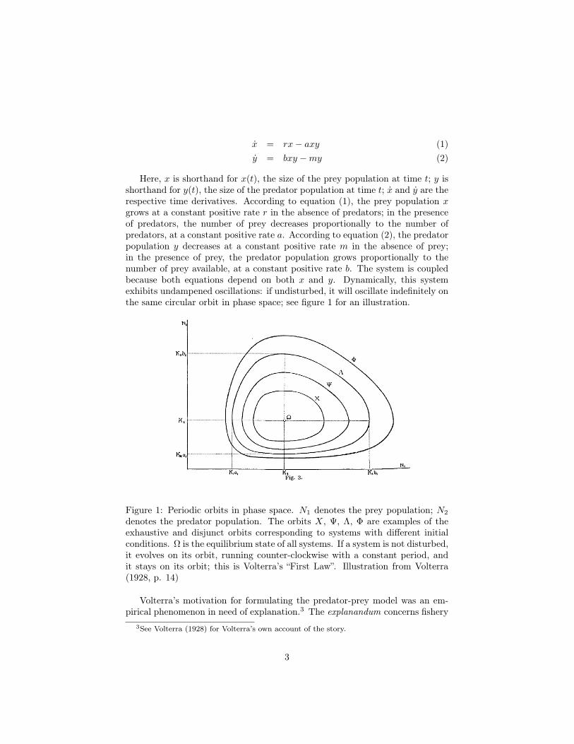
Here, x is shorthand for x(t), the size of the prey population at time t; y isshorthand for y(t), the size of the predator population at time t; x and y are therespective time derivatives. According to equation (1), the prey population xgrows at a constant positive rate r in the absence of predators; in the presenceof predators, the number of prey decreases proportionally to the number ofpredators, at a constant positive rate a. According to equation (2), the predatorpopulation y decreases at a constant positive rate m in the absence of prey;in the presence of prey, the predator population grows proportionally to thenumber of prey available, at a constant positive rate b. The system is coupledbecause both equations depend on both x and y. Dynamically, this systemexhibits undampened oscillations: if undisturbed, it will oscillate indefinitely onthe same circular orbit in phase space; see figure 1 for an illustration.

Figure 1: Periodic orbits in phase space. N1 denotes the prey population; N2

denotes the predator population. The orbits X, Ψ, Λ, Φ are examples of theexhaustive and disjunct orbits corresponding to systems with different initialconditions. Ω is the equilibrium state of all systems. If a system is not disturbed,it evolves on its orbit, running counter-clockwise with a constant period, andit stays on its orbit; this is Volterra’s “First Law”. Illustration from Volterra(1928, p. 14)

Volterra’s motivation for formulating the predator-prey model was an em-pirical phenomenon in need of explanation.3 The explanandum concerns fishery

3See Volterra (1928) for Volterra’s own account of the story.

3

statistics. During WW1, when fishing in the Adriatic was diminished, fisherystatistics showed that the ratio between predators and prey fish shifted in favorof predators. After the war, when fishing returned to its pre-war intensity, theratio shifted back, and favored the prey. This prompted the question as to whythis shift in proportions occurred. The explanation is provided by Volterra’s“Third Law”, now called the Volterra Principle. The Volterra Principle statesthat, if we continuously remove a constant proportion of both the predator andprey populations, then the average number of predators will decrease relativeto the average number of prey; see figure 2 for an illustration. Volterra showedthat this shift of averages can be derived from the predator-prey model. Hethus provided a how-possibly explanation of the statistical phenomenon: theregularity holds in a very simple model of population dynamics.4

It has, however, been disputed that the Volterra Principle provides an actualexplanation. Many mathematical population biologists today do not believe thatthe Lotka-Volterra model is a realistic model of predator-prey interactions. Themain mathematical problem with the model is that it is not structurally stable:if perturbations terms are added to the model equations, the model’s qualitativebehavior changes.5 Does this mean that the Volterra Principle is also doomed tofail? This question has been brought to philosophers’ attention in two papers:Michael Weisberg (2006b), and Michael Weisberg and Kenneth Reisman (2008).Weisberg and Reisman argue that the Volterra principle does not depend on thespecifics of the original predator-prey model. Rather, the Volterra Principle canbe derived from a variety of models, which are more realistic than the originalpredator-prey model. In short, Weisberg and Reisman claim that the VolterraPrinciple is a “robust theorem”. This makes the Volterra Principle a primeexample for the practice of robustness analysis. In the next section, I give abrief introduction to robustness analysis, as well as to Weisberg and Reisman’saccount of the Volterra Principle.

3 Robustness Analysis

3.1 Early ContributionsRobustness analysis was first discussed as a scientific practice in a seminal paperby Richard Levins (1966).6 Levins observes that population biology makes useof highly idealized models, i.e., the models are based on assumptions that are,strictly speaking, false with respect to their target systems. How can we makesure, nonetheless, that results we derive from such models are still true withrespect to their target systems, and not mere artifacts of the idealizations of themodels? Levins recommends robustness analysis as a remedy. The idea is toderive results from “several alternative models each with different simplifications

4See, e.g., Forber (2010); Scholl and Räz (2013) on the notion of how-possibly explanations.5See Brauer and Castillo-Chávez (2001, p. 180) for more on the notion of structural

stability.6See Weisberg (2006a) for an appraisal of Levins’ paper.

4

Figure 2: The population density of the predator-prey system with orbit Λ isat the equilibrium point Ω on average; this is Volterra’s “Second Law”. If theequations (1)-(2) of the system at point P are changed, such that the predatordeath rate m increases and the prey birth rate r decreases, the system evolveson the new orbit Λ′ with the equilibrium point Ω′. On average, system Λ′ hasa higher prey density (K1 to K ′1), and a lower predator density (K2 to K ′2).This is Volterra’s “Third Law”. Before and after WW1, the system was onorbit Λ′; during WW1, with greatly reduced fishing, the system was on orbit Λ.Illustration from Volterra (1928, p. 19).

but with a common biological assumption” (Levins, 1966, p. 423). If this pro-cedure is carried out successfully, the results are called “robust theorems”. Theslogan of robustness analysis is that “our truth is the intersection of independentlies” (Ibid.).

An early adopter of robustness analysis is William C. Wimsatt (2012b)[1981].7 Wimsatt advocates a wide conception of robustness analysis, alsodubbed “multiple determination”, whereby the practice is not restricted to thederivation of phenomena from different models, but rather encompasses, say, thedetection of phenomena using different senses, or different experimental meth-ods. Wimsatt emphasizes that it is important to determine the limitations ofrobustness results, given that robustness analysis involves, in part, understand-

7See also Wimsatt (2007).

5

ing the scope and limitations of the robustness of a phenomenon.An important critique of Levins’s proposal has been formulated by Steven

Hecht Orzack and Elliott Sober (1993). Orzack and Sober point out that ro-bustness analysis cannot play a confirmatory role. If all the models used inrobustness analysis are idealized, then we do not know whether results derivedfrom these models are true with respect to the target system. If we want to becertain, we would have to make sure that at least one of the models faithfullyrepresents the target system. However, this is usually not the case. In short,independent lies are still lies. In reaction to Orzack’s and Sober’s objection,Levins (1993) argues that he did not intend robustness analysis to provide non-empirical confirmation; rather, robustness analysis is merely supposed to helpin determining the scope and limits of a result.

3.2 Weisberg and ReismanThe most influential recent account of robustness analysis has been proposedby Michael Weisberg (2006b).8 Weisberg aims to reconcile robustness analysiswith the objections raised by Orzack and Sober. He proposes that robustnessanalysis does not confer full-blown confirmation, but rather “low-level confirma-tion”, that is, “confirmation of the fact that certain mathematical structures canadequately represent properties of target phenomena” (Ibid., p. 740). Weisbergcharacterizes robustness analysis as a four-step process. In the first step, oneexamines whether several distinct models share a property that is expected tobe robust. In the second step, one tries to identify the “core structure” thatis responsible for the robust property. The third step consists of an empiricalinterpretation of the mathematical structure. The fourth step consists of “sta-bility analysis”, with the purpose of finding out how sensitive the models are,with respect to slight changes to their structure.

Weisberg uses the Volterra Principle as a case study to support his analysis.He argues that the Volterra Principle is robust, given that it can be obtained indifferent predator-prey models.9 Specifically, Weisberg claims, we can modifythe structure of the original predator-prey model by adding density dependenceand predator satiation, and still obtain the Volterra Principle; see appendixA for a brief discussion of these models. Weisberg claims that the VolterraPrinciple can be shown to be valid for both of these models. Establishing thatthese two models satisfy the Volterra Principle corresponds to the first step ofrobustness analysis. Weisberg then argues that these models have a commonstructure: the growth rate of predators is mostly controlled by the growth rateof prey, and the growth rate of prey is mostly controlled by the death rate ofpredators. According to Weisberg, this common structure is responsible for thephenomenon that predators and prey are affected differently by continuous de-

8The interest in Levins’s paper, and robustness analysis, was renewed by Weisberg andJay Odenbaugh (2006). These papers initialized the “second wave” of robustness analysis. SeeWimsatt (2012a) for a useful account of the development of robustness analysis.

9Weisberg’s ideas are based on suggestive remarks in Roughgarden (1979), a textbook inpopulation ecology.

6

struction of both species. The identification of the common structure concludesstep two of robustness analysis.

Michael Weisberg and Kenneth Reisman (2008) push robustness analysisfurther, and they refine the results regarding the Volterra Principle. First, theydistinguish three kinds of robustness. Parameter robustness investigates ro-bustness with respect to a variation of parameters in a model. For example,the Volterra Principle is robust under variations of the parameters a, b, r, andm in the model (1)-(2). Structural robustness encompasses the more generalrobustness across models with different (causal) structure, e.g., models with orwithout density dependence.10 Representational robustness encompasses modelsthat are formulated in different frameworks, e.g., using continuous vs. discretevariables. Weisberg and Reisman then argue that the Volterra Principle is ro-bust according to all three kinds of robustness. They provide a formulation ofthe Volterra Principle that modifies the “hypothesis” from Weisberg (2006b).The new formulation is based on the notions of negative coupling and biocide.A predator-prey system is negatively coupled “just in case increasing the abun-dance of predators decreases the abundance of prey and increasing the abun-dance of prey increases the abundance of predators” (Weisberg and Reisman,2008, p. 114). In a general biocide, the death rate of predators is increased andthe birth rate of the prey is decreased.11 The new formulation of the VolterraPrinciple reads as follows:

(VP) Ceteris paribus, if a two-species, predator-prey system is negatively cou-pled, then a general biocide will increase the abundance of the prey anddecrease the abundance of predators. (Ibid., italics in original.)

Weisberg and Reisman claim that this principle holds in general. However,they do not provide a conclusive answer as to the scope and limits of (VP).Weisberg and Reisman also analyze further models with respect to the VolterraPrinciple. In Weisberg (2006b), robustness analysis was restricted to parameterand structural robustness – the models are all formulated in the framework ofcoupled ordinary differential equations – while Weisberg and Reisman (2008)also includes an analysis of individual-based models (IBM). These are finitemodels with discrete space and time, and representations of individual animals.In IBM, the discrete transition rules are not deterministic, but rather stochastic.The behavior of these models is investigated via simulations. Weisberg andReisman argue that the Volterra Principle can be recovered in this framework,and they therefore conclude that the Volterra Principle is representationallyrobust.

10Structural robustness is not to be confused with structural stability, a mathematical no-tion.

11In the case of system (1)-(2), r is decreased and m is increased. The notion is madeprecise in definition 1, see section 4.1 below.

7

3.3 After Weisberg and ReismanThe work by Weisberg and Reisman has renewed philosophers’ interest in ro-bustness analysis. Weisberg’s account of robustness analysis, and the notionof low-level confirmation, have received considerable attention. Brett Calcott(2011) points out that a robust theorem is only as good as the set of modelsfrom which it has been derived, and that this is not sufficient for confirmation.However, robustness can nevertheless be helpful by “narrowing down the pos-sibility space of candidate solutions” (Calcott, 2011). Wybo Houkes and KristVaesen (2012) provide an in-depth analysis of Weisberg’s work. The main lessonof their paper is that the evaluative role of robustness analysis concerning a setof models is only as good as the credibility of the model family from which theset of models is chosen. The idea of robustness analysis has been applied topure mathematics: Ralf Krömer (2012) discusses a potential role for robustnessin the foundations of mathematics, and; David Corfield (2010) focuses on math-ematical structures exhibiting a surprising “confluence” of structural properties.The idea of robustness analysis has also been applied to cases from biology inKnuuttila and Loettgers (2011), and to economics in Kuorikoski et al. (2010).

Robustness analysis is also relevant to the issue of scientific and mathe-matical explanation. The idea that robustness analysis can enhance our under-standing of a phenomenon was proposed early in the literature, e.g. by Wimsatt(2012b). However, the relevance of robustness analysis for explanation has notbeen systematically explored. A notable exception is a recent contribution byJonah Schupbach (2016). Schupbach proposes that robustness analysis can beinterpreted as an explanatory enterprise. The idea is that if we establish therobustness of a property, then we can rule out competing explanations of thatproperty. Schupbach illustrates the idea with the Volterra Principle. Initially,we should not be confident that the Volterra Principle is generally valid, be-cause we have only derived it from the original predator-prey model, and theresult could be due to the idealizations of this simple model. However, if wecan establish the Volterra Principle for models with different idealizations, then,according to Schupbach, we can rule out certain competing explanations as towhy the Volterra Principle holds, namely explanations attributing this fact toidealizations that are not present in the new models.

3.4 Robustness Analysis and MathematicsIn the present paper, I restrict my attention to one particular kind of robustness,namely the case of robust theorems that are derived from multiple, independentmodels. This is a special case of robustness, in comparison to the wider notion ofrobustness championed, for example, by Wimsatt.12 The focus of the discussionwill be on the role of mathematics in robustness analysis. While it has beenacknowledged in the philosophical discussion that mathematics has an importantrole to play in robustness analysis, a systematic exploration of this role is so farmissing from the discussion. I will strive to fill this lacuna here. I will argue

12See Calcott (2011) for a similar, useful distinction between several kinds of robustness.

8

that mathematics can help us enhance our confidence in a robust result byshowing that it does not depend on particular idealizations. However, this is notachieved by deriving the result from multiple, independent models, but rather byderiving the result from one, general model. I will not argue that mathematics,or robustness analysis, can play a confirmatory role. My discussion of robustnessanalysis is based on scientific practice: in the next section, I will present newresults concerning the Volterra Principle.

4 The Volterra Principle Generalized

4.1 The Volterra Principle in a Gause-type ModelIn the present section, I generalize the results in Weisberg (2006b) regarding theVolterra Principle. More specifically, I prove that the Volterra Principle holdsfor a more general type of model, which was first proposed by G. F. Gause(1934). I use the following modification13 of a Gause-type model:

x = xrf(x)− p(x)y (3)y = p(x)y −my (4)

x is prey abundance, y is predator abundance, r is the constant part ofthe prey growth rate, m is predator mortality. The prey growth rate functionf(x), which was missing in the original predator-prey model, is assumed to bedifferentiable for x ≥ 0; additionally, it is assumed that df

dx =: fx ≤ 0 andf(0) = a > 0. The environment can have a carrying capacity, i.e., a constantK > 0 with f(K) = 0. The functional response p(x), which was assumed tobe the identity function in the original predator-prey model, is assumed to bedifferentiable for x ≥ 0; additionally, it is assumed that dp

dx =: px > 0 andp(0) = 0.14

The Volterra Principle states how the equilibrium of a dynamical systemis affected by a change in the parameters of the system; see figure 2 above.In order for this to be biologically meaningful, the system (3) - (4) needs tohave an equilibrium inside the first quadrant, i.e., an equilibrium with positivepopulation variables. For the existence of such an equilibrium, we have toassume that there is an x∗ such that p(x∗) = m. For the formulation of theVolterra Principle, we additionally assume the existence of an x′ with p(x′) =m+ δ for a given δ > 0. x∗ and x′ are unique, because p(x) is increasing. If thesystem has a carrying capacity K, we have to assume that x∗, x′ < K for theexistence of an equilibrium.

The coordinates of the equilibrium in the first quadrant can be determinedas follows: We set equations (3) and (4) equal to 0 and solve the resulting

13See Freedman (1980, Ch. 4). In comparison to system (4.2), p. 66 of (Freedman, 1980),I use rf(x) instead of g(x) in equation (3), and p(x) instead of cp(x) in equation (4).

14The numerical response, p(x) in (4), is set equal to the functional response, p(x) in (3).See Freedman (1980, Ch. 4) for a further discussion of the significance of these assumptions.

9

equations. Using the assumption that there is a unique x∗ with p(x∗) = m, wecan deduce that the unique equilibrium has the following coordinates:

(x∗,x∗rf(x∗)

p(x∗)) (5)

The change in parameters, which leads to a change in equilibrium, can beinterpreted as an intervention. The following definition makes this precise:

Definition 1. A Volterra Intervention in a predator-prey system is a decreaseof r by an amount ε, with 0 < ε < r, and an increase of m by an amount δ > 0.

The assumption that 0 < ε < r avoids a negative growth rate. 0 < δ yields anew, unique equilibrium in the positive quadrant after the Volterra Intervention.If we apply a Volterra Intervention to equilibrium (5), and use p(x′) = m + δ,we get a unique equilibrium with the following coordinates:

(x′,x′(r − ε)f(x′)

p(x′)) (6)

We are interested in the relation between the equilibrium (5) and the equi-librium (6); more specifically, how a Volterra Intervention affects the relativeabundance of the populations:

Definition 2. A predator-prey system has the Volterra Property if a VolterraIntervention, applied to an equilibrium (x∗, y∗), yields an equilibrium (x′, y′)such that the equilibrium abundance of predators relative to prey, i.e., theirratio, decreases: y∗

x∗ >y′

x′

If we examine figure 2, we see that the original Lotka-Volterra model hasthe Volterra Property: K2

K1>

K′2K′1

is true because K2 > K ′2 and K1 < K ′1. Weare now in the position to formulate the following:

Theorem 1. For Gause-type models (3) - (4), the Volterra Property holds true.

Proof. We have to show that the Volterra Property holds true for the system(3) - (4), i.e, the ratio y∗/x∗ from equilibrium (5) is bigger than the ratio y′/x′from equilibrium (6):

rf(x∗)

p(x∗)>

(r − ε)f(x′)

p(x′)(7)

This inequality can be rearranged to yield

f(x∗)

f(x′)

p(x′)

p(x∗)> 1− ε

r(8)

Because p(x∗) = m, p(x′) = m + δ and because p is strictly increasing, weknow that x′ > x∗, i.e., x′ = x∗ + κ for some κ > 0. Replacing x′ with x∗ + κ,we see that (8) is equivalent to

10

f(x∗)

f(x∗ + κ)

p(x∗ + κ)

p(x∗)> 1− ε

r(9)

The fact that f is a decreasing function implies that f(x∗)/f(x∗+κ) ≥ 1, andthe fact that p is a strictly increasing function implies that p(x∗+κ)/p(x∗) > 1.This implies that the LHS of the inequality is bigger than 1. The RHS, on theother hand, is smaller than 1 for ε > 0. Therefore, the inequality holds true.

4.2 Stable EquilibriaTheorem 1 is a statement about how the equilibrium of a system changes undera Volterra Intervention. However, this is not sufficient for the result to bebiologically meaningful. The existence of an equilibrium does not guaranteethat the average abundance of a system coincides with the equilibrium. In thecase of the original Lotka-Volterra model, this was guaranteed by Volterra’s“Second Law”; see figure 2 above. However, other predator-prey models show avariety of qualitatively different behaviors. For example, the so-called Samuelsonmodel15 has an equilibrium that is stable or unstable depending on the choice ofparameters. For some choices, the system spirals towards a stable equilibrium inthe first quadrant. For other choices, the system spirals away from an unstableequilibrium. In the latter case, it is not relevant whether or not the VolterraPrinciple holds true, because the equilibrium point is not where the system isusually, or on average. Rather, the system will show more and more violentfluctuations, such that the equilibrium shift predicted by the Volterra Principleis irrelevant. The same problem also occurs in models with limit cycles. Forexample, the model with predator satiation examined in Weisberg (2006b, p.736) satisfies the Volterra Princile according to Theorem 1. However, the systemdoes not converge towards an equilibrium, because the model exhibits limitcycles, and it is not clear how average abundance and equilibrium are related –an additional result analogous to Volterra’s “Second Law” would be necessaryto establish such a relation.

One way of making sure that the equilibrium is biologically relevant is torequire that it is stable.16 Stability questions are standard in mathematicalpopulation ecology, and Theorem 1 can be combined with an available stabilitycriterion. An eigenvalue analysis of generalized Gause systems yields a crite-rion for the equilibrium’s stability.17 This criterion implies that the relevantequilibrium of the system (3) - (4) is stable under the following condition18:

H(x∗) = x∗fx(x∗) + f(x∗)− x∗f(x∗)px(x∗)

p(x∗)< 0 (10)

15See Freedman (1980, pp. 37) for a discussion of this model.16The relevant notion here is asymptotic stability, which means that systems close to equi-

librium will eventually converge to that equilibrium. This is not to be confused with structuralstability mentioned above. See Freedman (1980); Kot (2001) for more on asymptotic stability.

17See Freedman (1980, p. 72, condition (4.23)).18fx(x∗), px(x∗) is the derivative of f, p with respect to x, evaluated at x∗.

11

This condition can be combined with Theorem 1 as follows: If the equilibriumof the system (3) - (4), before and after the Volterra Intervention, is stableaccording to condition (10), then Theorem 1 is certainly biologically meaningful.

4.3 The Limits of the Volterra PrincipleAn important advantage of Theorem 1 is that condition (9) allows us to inferthe limits of the Volterra Principle. In particular, condition (9) shows how theproof of the theorem depends on the assumptions about functions f and p, andit also shows that these assumptions are minimal, in that if they are weakenedfurther, the theorem does not hold. Here I will discuss two ways in which theVolterra Principle does not hold if the assumptions on f and p are weakened.

Possibility 1: Assume that fx > px > 0 in a range x ∈ [x∗, x∗ + κ], i.e., fis no longer decreasing, but increasing faster than p. This implies that the LHSof (9) gets smaller than 1 and the inequality is violated for sufficiently small ε.

Possibility 2: Assume that px < 0, i.e., the functional response decreases.In this case, we have to be more careful, because the theorem depends on px > 0in several places. First, we used that px > 0 implies the uniqueness of theequilibrium. If px < 0, there could be two equilibria, or none. Second, we usedpx > 0 to infer x′ > x∗. If px < 0, this relation is inverted; this leads to amodification of condition (9):

f(x∗)

f(x∗ − κ)

p(x∗ − κ)

p(x∗)> 1− ε

r(9’)

If we assume that p does not change sign, we need fx > |px| > 0 in the rangex ∈ [x∗ − κ, x∗] in order to violate inequality (9’), i.e., f has to increase fasterthan p is decreasing.19

Are the conditions, under which the Volterra Principle is violated, biolog-ically realistic? Consider, first, possibility 1. fx > 0 is not realistic globally,because it implies unbounded growth of prey in the absence of predators. How-ever, fx > 0 seems reasonable in a limited range, in particular when the preypopulation is small and growth is not restricted externally. Turning to possibil-ity 2, the case of a decreasing functional response p has been discussed in theliterature; see, e.g., Kot (2001, pp. 140). According to Kot, so-called “type IV”functional responses can occur due to prey interference or prey toxicity. Thus,both possibilities potentially occur in situations that are biologically realistic.

It could be asked whether the assumptions of Theorem 1, on the one hand,and the requirement of stable equilibria, on the other, are independent. Does thetheorem exclude unstable equilibria, or can we find predator-prey models thatviolate the Volterra Principle and have stable equilibria at the same time? In

19If we use a function q(x) instead of p(x) in the predator equation (4) in the model, thereare more possibilities for violating the Volterra Principle – a decreasing q, combined withincreasing p and decreasing f , yields a violation of the Volterra Principle. However, it isunclear how realistic it is to assume that the functions p and q show a qualitatively differentbehavior.

12

order to answer this question, it is useful to reformulate the stability condition(10). If we assume that f(x∗) is not 0, (10) is equivalent to

fx(x∗)

f(x∗)− px(x∗)

p(x∗)< − 1

x∗(11)

The expression on the LHS contains statements about the relative change inf and p. The question now is whether there are cases in which condition (11)holds true, while condition (9) is violated. Consider possibility 1 of violating (9),viz. fx > px > 0. This is compatible with stability (11) if f(x∗) is sufficientlybig, while p(x∗) is sufficiently small. Turning to possibility 2, viz. fx > |px| > 0,and px < 0, we see that we cannot get stability, because the LHS of (11) will bepositive, unless we admit negative functional responses. This shows that thereare models with stable equilibria that violate the Volterra Principle, notablymodels that violate the Volterra Principle according to possibility 1.

4.4 Further GeneralizationsCan the above results be generalized further? Theorem 1 depends on the scopeof system (3) - (4). This type of model is dubbed “intermediate” in Freedman(1980). There is a lot of space for generalization between Gause-type modelsand fully general dynamical systems.20 Here I want to mention a different kindof intermediate model that is important in population ecology. The system (3) -(4) has so-called “laissez-faire” dynamics, i.e., the functional response (which isalso the numerical response) p(x) does not depend on the predator abundancey. Some population ecologists believe that this is problematic, because thesemodels do not allow for non-trivial predator interference.21 To overcome theproblems of “laissez-faire” dynamics, Roger Arditi and Lev Ginzburg (1989)have proposed so-called ratio-dependent predator-prey models, in which thefunctional and numerical responses are functions of the ratio between predatorand prey abundances. Ratio-dependent models have been hotly debated inpopulation ecology in recent decades.22 It would be interesting to see whetherthe Volterra Principle can be extended to this type of model as well.

5 Weisberg’s Volterra Principle RevisitedIn this section, I discuss the ramifications of the results in section 4 for Weis-berg and Reisman’s work on the Volterra Principle, as far as the scientific and

20A general approach to predator-prey models is via so-called Kolmogorov-type models;see, e.g., Freedman (1980, Ch. 5). This approach was first proposed by Andrey Kolmogorov(1978) [1936]. Kolmogorov-type models take general dynamical systems of two variables as astarting point and impose certain restrictions on these systems in order to obtain predator-preyrelationships.

21See Peter Yodzis (1994) for a discussion of the notion of “laissez-faire” dynamics, andreasons for taking predator interference into account.

22See Arditi and Ginzburg (2012) for a book-length discussion, and Barraquand (2014) fora critical evaluation, of ratio-dependent models.

13

mathematical substance of their contribution is concerned. First, the fact thatthe Volterra Principle holds for models with density dependence and predatorsatiation, which was pointed out by Weisberg, is implied by Theorem 1: onemerely has to observe that these models are special cases of (3) - (4); see ap-pendix A. What is more, Theorem 1 not only shows that these two modelssatisfy the Volterra Principle, but also shows that this is due to the propertiesof the form of the growth function f , and of the functional and the numericalresponse p. I will turn to the ramifications of these observations for robustnessanalysis below.

Second, the analysis of the scope of Theorem 1, provided in section 4.3,shows that (VP), the formulation of the Volterra Principle in Weisberg andReisman (2008), is incorrect. This is particularly clear if we consider possibility1, according to which a violation of the Volterra Principle can occur if the growthfunction f is increasing. However, f is independent of negative coupling, whichonly concerns the interaction terms. Therefore, the Volterra Principle can beviolated if there is negative coupling, and (VP) is wrong.

Third, the equilibrium of a predator-prey system need not necessarily be the(average) abundance of that system, as I noted in section 4.2 above. Weisbergand Reisman do not explicitly address this problem. I already pointed outthat Weisberg (2006b, p. 736) proposes extending the Volterra principle to amodel with predator satiation; see appendix A. This model satisfies the VolterraPrinciple, according to Theorem 1. However, the model exhibits limit cycles.An argument analogous to Volterra’s “Second Law” would be necessary to showthat the equilibrium of this system is relevant to the average abundance; withoutsuch an argument, the Volterra Principle may be irrelevant. There is no suchargument in Weisberg (2006b). To be fair, Weisberg and Reisman (2008, p.119) implicitly acknowledge that the stability of equilibria is relevant to theVolterra Principle. They compare the significance of equilibria, in the case ofthe original Lotka-Volterra predator prey model, one the one hand, and in thecase of the model with density dependent prey, on the other, and note that inthe former case, the equilibrium is the average abundance, while in the lattercase, the system will actually converge towards the equilibrium. They seem toendorse the system being at equilibrium (at least on average) as a necessarycondition for the Volterra Principle’s being biologically meaningful.

6 Robustness Analysis and GeneralizationWhat is the upshot of the results in section 4 for robustness analysis, and Weis-berg’s (2006b) account in particular? Weisberg proposes that robustness anal-ysis proceeds in four steps; see section 3. The results in section 4 are purelymathematical, and they are thus located within the first two steps of Weisberg’saccount. However, the results in section 4 deviate from Weisberg’s recipe in thesecond step. I did not explore the common structure of the different models;instead, I introduced one general model, the Gause-type model, which encom-passes all the different models from Weisberg (2006b). I then showed that the

14

Gause-type model has the Volterra Property. This generalization shows that themodels investigated by Weisberg are not really independent, but rather belongto the same type, and that they all satisfy the Volterra Principle, because theyare of this type.

Weisberg anticipates that something along these lines is a possible outcomeof robustness analysis. In the description of the second step, he writes:

In straightforward cases, the common structure is literally thesame mathematical structure in each model. In such cases one canisolate the common structure and, using mathematical analysis, ver-ify the fact that the common structure gives rise to the robust prop-erty. However, such a procedure is not always possible because mod-els may be developed in different mathematical frameworks or mayrepresent a similar causal structure in different ways or at differentlevels of abstraction. Such cases are much harder to describe in gen-eral, relying as they do on the theorist’s ability to judge relevantlysimilar structures. (Weisberg, 2006b, p. 738)

The generalization approach pursued in section 4 is such a “straightforwardcase”. The Volterra Principle turned out to be an actual theorem for the Gause-type model. I agree with Weisberg that such an outcome should not be expectedin all cases. However, there are systematic differences between cases in whichwe can expect to obtain a mathematical theorem, as opposed to cases where notheorems are forthcoming. I will now identify some of these differences.

The generalization approach will usually not work if models are from dif-ferent mathematical frameworks, as Weisberg notes. The results in section 4concern models that are ordinary differential equations. Their robustness isthus restricted to this particular mathematical framework, and does not ex-tend to, say, individual-based models, as explored in Weisberg and Reisman(2008). Put differently, the generalization approach does not work in the case ofrepresentational robustness, i.e., when models belong to different mathematicalframeworks. The reason for this is that models belonging to different frame-works usually do not share a common mathematical structure, and it is hard, ifnot impossible, to treat them in a formally unified manner. The generalizationapproach is usually restricted to cases of structural robustness, i.e., robustnessfor models from the same mathematical framework.

It is not sufficient, however, that the models are formulated within the samemathematical framework for the generalization approach to be applicable. Itcan be impossible to find a common generalization of models, even if they areformulated in the same mathematical framework. For example, Vito Volterra(1978) [1927] explores properties of population fluctuations; the third property,the “disturbance of averages”, is the Volterra Property. In Part Two, §5, Volterrageneralizes the Volterra Principle to systems with n species. Volterra notes that,in order for this to make sense, one has to restrict n-species models in severalways. For example, if one wants to be able to compare the abundances of preda-tors and prey, one needs an absolute distinction between predators and prey.

15

Cases where one species is preyed upon by a second species, whilst also itselfbeing the predator of a third species, have to be excluded, because it is notclear how the Volterra Principle should even be formulated in such cases. How-ever, Volterra shows that, under certain technical assumptions, a generalizedanalogue of the Volterra Principle can be proven if the system contains an equalnumber of predator and prey species. This draws attention to an importantaspect of the generalization approach: the precise formulation of the propertythat is expected to be robust is important. In the cases examined by Volterra,the robust property is not the same for two species and for n-species systems. Inthe former case, the property is formulated in terms of the ratio of two species,whereas in the latter case, the property concerns the ratio of (equally many)predator and prey species. Thus, the generalization approach can be difficultto carry out, if the robust property is not the same in all cases and needs to bereformulated.

In the case of the models examined in Weisberg (2006b), which served as thestarting point of the generalization approach, we find that the robust propertyin question, the Volterra Property, is the same formal statement in all cases.This is not an assumption that is generally made in robustness analysis. Gener-ally, a robust property can be characterized informally, and the statements areonly required to be similar, or “biologically the same”. A second commonality ofthe models examined in Weisberg (2006b) is that the derivations of the VolterraProperty, while different, are similar. I suggest that in this kind of situation,the generalization approach should be applied as a rule of thumb: if a series ofmodels, formulated in the same mathematical framework, yields identical for-mulations of a robust property, and the derivations proceed in a similar manner,we should try to identify one general model from which we can derive the ro-bust property. In this kind of situation, robustness analysis serves as a heuristicstrategy: the point of deriving the same result from a range of different modelsserves the ultimate goal of finding a general result, by examining some instancesfirst.

So far, we have seen that the generalization approach deviates from the usualsteps of robustness analysis, in that it results in one general model instead ofmultiple, independent models. We have also identified conditions under whichthe generalization approach may be applicable. I will now turn to the questionas to whether robustness analysis and the generalization approach are compat-ible. The goal of robustness analysis is to solve the following problem: if weuse an idealized model, such as the original Lotka-Volterra model, to derive aregularity, such as the Volterra Principle, we do not know whether this resultapplies to the target system, or whether it is a mere artifact of the idealizationsof the model. The solution is to establish the Volterra Principle for multiple,independent models, to make sure that the result is independent of the ideal-izations of the original model. The goal of the generalization approach is thesame, namely to show that a result, such as the Volterra Principle, does notdepend on the idealizations of a particular model. However, the generalizationapproach shows that the idealizations of the original model are not necessary;weaker assumptions suffice to derive the same result. Note that generalization

16

does not get rid of all idealizations. The generalization of a result is only as goodas the idealizations used in the general model. The two approaches, then, sharethe goal of controlling for idealizations, but they achieve this goal in differentways: the generalization approach uses one, general model, while robustnessanalysis uses multiple, independent models to control for idealizations.

7 The Generalized Volterra Principle as an Ex-planation

The Volterra Principle was originally proposed as an explanation of an empiricalregularity, as I pointed out in section 2 above. It is, therefore, natural to askwhether the results in section 4 are explanatorily significant. I discuss thisissue in the present section. I show that the results in section 4 exhibit severalexplanatory virtues that have been proposed in the debate on mathematicalexplanations.

Before I discuss the explanatory virtues, some clarifications are in order.The original explanandum is an empirical regularity observed in fishery statis-tics. These findings have been disputed on empirical and statistical grounds,e.g. by E.S. Pearson (1927). Of course, the facticity of the explanandum is nec-essary if we want to give a real explanation.23 Here I do not discuss empiricalquestions, but I rather assume that we are dealing with an actual, empiricalphenomenon. I then assess the theoretical virtues of the results in section 4under this assumption. The explanation I discuss is that the Volterra Propertyin Gause-type models is explained by the fact that the growth rate function fis decreasing, whilst the functional response p is increasing.

One of the explanatory virtues of the above results consists in their gener-ality, or unificatory power, and we can spell this out in terms of unification, asproposed by Philip Kitcher (1989): if we compare Weisberg’s results with thosegiven here, we see that the explanation I propose is more unified, and that itsubsumes different, but similar, arguments given by Weisberg, under one argu-ment scheme, in a natural way. Now, it has been argued in the literature onmathematical explanations that unification, and generality, cannot be all thereis to mathematical explanation.24 I agree that while generality and unificationdo contribute to explanatory power, they are not all there is to it.

A second explanatory virtue of the results in section 4 is that the resultsestablish natural boundaries for the validity of the Volterra Principle.25 I showedthat the Volterra Principle is not valid if the assumptions on the functions f and

23Additionally, one should always compare the mechanism producing the empirical phe-nomenon with the model used in the explanation, in order to assess the explanation’s ade-quacy.

24See Hafner and Mancosu (2008) for a critical discussion of unification à la Kitcher in thecontext of mathematical explanation, and Steiner (1978) for arguments against a characteri-zation of explanatory power in terms of generality.

25The importance of establishing the limits of a result to robustness analysis has been madeby Wimsatt (2012b) [1981].

17

p are weakened any further. These properties are minimal, in that if the growthrate f increases, the explanandum does not follow; similarly, the equilibriummay become unstable, if the functional response p decreases. These propertiesare not only sufficient, but also necessary, for the Volterra Principle, againstthe background of Gause-type models. This fits nicely with a recent proposalby Christopher Pincock (2014), who requires conditions that are necessary aswell as sufficient for “abstract explanations”; a kind of mathematical explanation.Pincock’s idea is that requiring the condition to be necessary as well as sufficientmakes sure that there are no redundant assumptions in the explanans, in thatif the assumptions are weakened, the explanation fails. This is exactly what wesee here.

A third explanatory virtue of the Gause-type explanation emerges, if we an-alyze its relation to the other, less general explanations. Volterra’s explanation,based on the original predator-prey model, establishes that it is possible to ac-count for the Volterra Property, on the basis of systems of coupled differentialequations. Weisberg showed that Volterra’s result can be extended to other,more realistic models. This establishes that the explanation is not an artifactof the idealizations of the original predator-prey model. What the explanationbased on the Gause-type model achieves is the identification of the propertiesthat are ultimately responsible for the explanandum, viz. the (mathematical)Volterra Property. By doing this, the Gause-type explanation not only accountsfor the explanandum, but it also explains why the other explanations, proposedby Volterra and Weisberg respectively, worked in the first place: the growthfunction and the functional response of all these explanations have the rightproperties. The idea that explanatory relations of this kind, between differ-ent explanations, can be interpreted as an explanatory virtue has recently beenproposed by Marc Lange (2014). According to Lange, a mathematical resultthat answers questions that other results leave open is “deep”, and has highexplanatory power. This is a further important feature of the results presentedhere.

In sum, the results regarding the Volterra Principle presented above, haveseveral explanatory virtues. They are general, they provide an explanans that issufficient and necessary in the case of Gause-type models, and they are “deep”,in explaining why previous explanations worked.

8 Robustness Analysis and CoincidenceThe generalized Volterra Principle unifies multiple, apparently independent,models using the Gause-type model. This general model explains the VolterraProperty, and it also explains why we succeeded in deriving the Volterra Prop-erty from the other, apparently independent, models. While it is desirable toapply the generalization approach in other cases as well, there is no guaran-tee that it will always work. What if the generalization approach yields noresult? In the present section, I address this question. I will argue that in casesin which generalization cannot be applied, robustness analysis and explanation

18

pull in different directions. I will restrict attention to cases where generalizationis a promising approach in principle, i.e., cases where the same mathematicalstatement is derived from multiple, independent models within the same math-ematical framework.

Consider, for a moment, the reasoning process of a theorist who wants toestablish the robustness of a property, such as the Volterra Property. Thetheorist examines a range of different models within the same mathematicalframework, and succeeds in deriving the same property from different models.In this situation, the theorist can be confident that the property is in factrobust. However, the theorist will not stop there. She will also wonder whetherthe fact that she succeeded in deriving the result in such a way has a commonexplanation. In fact, there is a certain urgency to find such an explanation,because this would account for the fact that multiple derivations are possible.If, on the other hand, no such explanation is to be had – what does this tell us?It may tell us that the existence of multiple derivations is a mere coincidence.

It could be questioned whether mathematical coincidences are possible at all,given that all mathematical truths are necessary. At the very least, the notionof a mathematical coincidence needs to be clarified. The notion of mathematicalcoincidence has been discussed by Marc Lange (2010). Lange gives the followingexample of a mathematical coincidence: The thirteenth digit of the decimalexpansion of both e and π is 9. There is no reason, or common explanation, forthis fact; at least, no such explanation is known. It is a mere coincidence. In anutshell, Lange’s account of mathematical coincidence is that two mathematicalfacts F and G are coincidences, if there is no common mathematical explanationof F and G. If we want this definition to be non-trivial, we have to make somerequirements on the “naturalness” that a common mathematical explanationwould have to satisfy; otherwise, a mere conjunction of any two explanationswould be sufficient. One of the main challenges is to spell out just what sucha requirement of “naturalness” amounts to. I will not discuss this issue in theabstract, but I will rather turn to the case at hand instead.

Lange’s idea applies to the case of the Volterra Principle, as follows. Themathematical coincidence is that we can derive the Volterra Property from theoriginal predator-prey model, as well as from both the model with density de-pendence, and the model with predator satiation; all of this was establishedin Weisberg (2006b). This situation, the (apparent) coincidence, prompts therequest for an explanation. The explanation is provided in section 4 above:the different models are special cases of the Gause-type model, from which theVolterra Property can be derived.26 Thus, in some cases, the process of robust-ness analysis can itself prompt a request for an explanation, and in a subset ofthese cases – including the generalized Volterra Principle – an explanation canbe provided, and the apparent coincidence is explained away.

What about real coincidences? In these cases, we succeed in deriving the26I am not suggesting here that all mathematical explanations have the form of general-

izations, or unification; I merely claim that the results in section 4 do in fact explain the(apparent) coincidence in Weisberg (2006b), viz. that the Volterra Property can be derivedfrom multiple models.

19

same property from multiple models, but there is no common explanation ofthe fact that these multiple derivations were possible. This fact is a mere co-incidence. In this case, the following situation arises. Assume that we wantto check whether some idealizations in a model M are responsible for the ex-planation of a property P , or whether the explanation is independent of theseidealizations. According to Schupbach (2016), we can do this using robustnessanalysis. Assume, further, that: we construct two models, M1 and M2, that;in these two models, different idealizations from M are removed, and that; wesucceed in deriving the property P from M1 and M2. Assume, finally, that thisis a mathematical coincidence. This means that there is no explanation as towhy we succeeded in deriving the property P from M1 and M2. If this is thecase, we will not be able to construct a model M ′ which encompasses M1 andM2, and from which we can derive P , insofar as such a derivation constitutes anexplanation telling us why the multiple, independent derivations are possible.This, in turn, means that the different idealizations in M , which were removedin M1 and M2 individually, cannot be removed collectively by constructing onemodel M ′, such that M ′ would explain P . This is worrisome because havingat least one of the idealizations seems to be essential to the derivation of theproperty P : it is impossible to remove all the idealizations in the two modelsat the same time by constructing an explanatory model. Note that the ex-planatory goal of robustness analysis, according to Schupbach’s proposal, canstill be achieved to a certain degree. We can control for some idealizations ina model, by deriving a property from different models, thus ruling out theseidealizations as explanations. However, some idealization cannot be removedfrom our explanation.

In sum, it has to be expected that generalization will not work in all cases.The interpretation of such cases as mathematical coincidences has interestingconsequences, in particular the impossibility of finding a general, explanatorymodel that removes all idealizations we would like to control for. This does notmean that generalization, or mathematical coincidences, speak against robust-ness analysis. Rather, we should interpret robustness analysis as a heuristicstrategy that can lead to several possible outcomes. On the one hand, we maydiscover a general model that provides a unified explanation of a mathematicalfact. On the other hand, however, we may find a mathematical fact that can bederived from several, independent models is merely an example of a mathemat-ical coincidence. In the latter case, the outcome of robustness analysis is thatan explanation is not to be had, and that some idealizations are here to stay.

9 ConclusionIn the present paper, I have shown that the Volterra Principle can be gener-alized for Gause-type models, extending results by Weisberg and Reisman. Ihave argued that this generalization has some of the virtues of mathematicalexplanations; in particular, the limits of the results establish necessary and suf-ficient conditions, and the results illuminate previous explanations. I have also

20

proposed that cases in which the generalization approach is not applicable canbe interpreted as mathematical coincidences.

The present paper reveals a close connection between the goals of robustnessanalysis and those of purely mathematical work on theoretical models. General-izing existing results is a very common practice in mathematics. However, thereare other aspects of mathematics that should also be explored in the context ofrobustness analysis. First, more should be said about cases of representationalrobustness, where the robust results stem from different mathematical frame-works. These are cases of analogical reasoning in mathematics, the status ofwhich is all but clear. Second, more complicated cases of structural robustnesshave scarcely been discussed so far. For example, a systematic study of “analog-ical generalizations”, such as Volterra’s generalizations of the Volterra Principleto n-species systems, would be worthwhile. Third, the results in the presentpaper could also be further generalized to other kinds of predator-prey models.

A Models with Density Dependence and Preda-tor Satiation

After normalizing parameters a and b, the model with density dependent prey(Weisberg, 2006b, equations (6)-(7)) can be written as

x = xr(1− x

K

)− xy (12)

y = xy −my (13)

In this model, the first summand in equation (1) is modified such that theprey population does not grow indefinitely in the absence of predators, butrather the growth is limited by a maximal number of prey, the carrying capacityK. This model can be seen to be of Gause-type by letting f(x) = 1 − x

K andp(x) = x.

The model with predator satiation (Weisberg, 2006b, equations (9)-(10)),after normalizing parameters a, b and c, can be written as

x = xr(1− x

K

)− (1− e−x)y (14)

y = (1− e−x)y −my (15)

This model takes into account that the rate at which predators capture preymay not be constant, as in the Lotka-Volterra model, but may rather decreasewith increasing prey density. This model can be seen to be of Gause-type, bychoosing f(x) = 1− x

K and p(x) = 1− e−x.

21

ReferencesArditi, R. and L. R. Ginzburg. 1989. Coupling in Predator-Prey Dynamics:Ratio-Dependence. Journal of Theoretical Biology 139(3): 311–26.

———. 2012. How Species Interact: Altering the Standard View on TrophicEcology. New York: Oxford University Press.

Barraquand, F. 2014. Functional responses and predator-prey models: a critiqueof ratio dependence. Theoretical Ecology 7: 3–20.

Brauer, F. and C. Castillo-Chávez. 2001. Mathematical Models in PopulationBiology and Epidemiology, vol. 40 of Texts in Applied Mathematics. NewYork: Springer.

Brewer, M. and B. Collins, eds. 1981. Scientific Inquiry in the Social Sciences.San Francisco: Jossey-Bass.

Calcott, B. 2011. Wimsatt and the robustness family: Review of Wimsatt’sRe-engineering Philosophy for Limited Beings. Biology and Philosophy 26:281–93.

Corfield, D. 2010. Understanding the Infinite I: Niceness, Robustness, and Re-alism. Philosophia Mathematica 18(3): 253–75.

Forber, P. 2010. Confirmation and explaining how possible. Studies in Historyand Philosophy of Science Part C 41: 32–40.

Freedman, H. I. 1980. Deterministic Mathematical Models in Population Ecol-ogy, vol. 57 of Pure and Applied Mathematics. New York, Basel: MarcelDekker, Inc.

Gause, G. F. 1934. The Struggle for Existence. Baltimore: The Williams &Wilkins Company.

Hafner, J. and P. Mancosu. 2008. Beyond Unification. In Mancosu (2008), pp.151–78.

Houkes, W. and K. Vaesen. 2012. Robust! Handle with Care. Philosophy ofScience 79: 1–20.

Kitcher, P. 1989. Explanatory Unification and the Causal Structure of theWorld. In Kitcher and Salmon (1989), pp. 410–505.

Kitcher, P. and W. C. Salmon, eds. 1989. Scientific Explanation, vol. XIII ofMinnesota Studies in the Philosophy of Science. Minneapolis: University ofMinnesota Press.

Knuuttila, T. and A. Loettgers. 2011. Causal isolation robustness analysis: thecombinatorial strategy of circadian clock research. Biology and Philosophy26: 773–91.

22

———. 2016. Modelling as Indirect Representation? The Lotka-Volterra ModelRevisited. British Journal for the Philosophy of Science .

Kolmogorov, A. 1978. On Volterra’s theory of the struggle for existence. In F. M.Scudo and J. R. Ziegler, eds., The Golden Age of Theoretical Ecology: 1923-1940, vol. 22 of Lecture Notes in Biomathematics. Berlin, Heidelberg, NewYork: Springer-Verlag, pp. 287–92. Translation of ’Sulla theoria di Volterradella lotta per l’esistenza’, 1936.

Kot, M. 2001. Elements of Mathematical Ecology. Cambridge: CambridgeUniversity Press.

Krömer, R. 2012. Are We Still Babylonians? The Structure of the Foundationsof Mathematics from a Wimsattian Perspective. In L. Soler, ed., Character-izing the Robustness of Science, Boston Studies in the Philosophy of Science,chap. 8. Springer, pp. 189–206.

Kuorikoski, J., A. Lehtinen, and C. Marchionni. 2010. Economic Modellingas Robustness Analysis. British Journal for the Philosophy of Science 61:541–67.

Lange, M. 2010. What Are Mathematical Coincidences (and Why Does ItMatter)? Mind 119: 307–40.

———. 2015. Depth and Explanation in Mathematics. Philosophia Mathematica23(2): 196–214.

Levins, R. 1966. The Strategy of Model Building in Population Biology. Amer-ican Scientist 54(4).

———. 1993. A Response to Orzack and Sober: Formal Analysis and theFluidity of Science. The Quarterly Review of Biology 68(4): 547–55.

Mancosu, P., ed. 2008. The Philosophy of Mathematical Practice. Oxford, NewYork: Oxford University Press.

Odenbaugh, J. 2006. The Strategy of ‘The Strategy of Model Building in Pop-ulation Biology’. Biology and Philosophy 21: 607–21.

Orzack, S. and E. Sober. 1993. A Critical Assessment of Levins’s The Strategyof Model Building in Population Biology (1966). The Quarterly Review ofBiology 68(4): 533–46.

Pearson, E. 1927. The application of the theory of differential equations tothe solution of problems connected with the interdependence of species.Biometrika 1(19): 216–22.

Pincock, C. 2015. Abstract Explanations in Science. British Journal for thePhilosophy of Science 66(4): 857–82.

23

Roughgarden, J. 1979. Theory of Population Genetics and Evolutionary Ecology:An Introduction. New York: Macmillan.

Scholl, R. and T. Räz. 2013. Modeling causal structures. European Journal forPhilosophy of Science 3(1): 115–32.

Schupbach, J. N. 2016. Robustness Analysis as Explanatory Reasoning. BritishJournal for the Philosophy of Science .

Steiner, M. 1978. Mathematical Explanation. Philosophical Studies 34(2): 135–51.

Volterra, V. 1928. Variations and fluctuations of the number of individuals inanimal species living together. J. Cons. int. Explor. Mer 3(1): 3–51.

———. 1978. Variations and fluctuations in the numbers of coexisting animalspecies. In F. M. Scudo and J. R. Ziegler, eds., The Golden Age of TheoreticalEcology: 1923-1940, vol. 22 of Lecture Notes in Biomathematics. Berlin, Hei-delberg, New York: Springer-Verlag, pp. 65–236. Translation of ’Variazioni efluttuazioni del numero d’individui in specie animali conviventi’, 1927.

Weisberg, M. 2006a. Forty years of “The strategy”: Levins on model buildingand idealization. Biology and Philosophy 21: 623–45.

———. 2006b. Robustness Analysis. Philosophy of Science 73(5): 730–42.

Weisberg, M. and K. Reisman. 2008. The Robust Volterra Principle. Philosophyof Science 75(1): 106–31.

Wimsatt, W. C. 2007. Re-Engineering Philosophy for Limited Beings. HarvardUniversity Press.

———. 2012a. Robustness: Material, and Inferential, in the Natural and HumanSciences. In L. Soler, ed., Characterizing the Robustness of Science, BostonStudies in the Philosophy of Science, chap. 3. Springer, pp. 89–104. From M.Brewer and B. Collins, eds., (1981).

———. 2012b. Robustness, Reliability, and Overdetermination. In L. Soler, ed.,Characterizing the Robustness of Science, Boston Studies in the Philosophyof Science, chap. 2. Springer, pp. 61–87. From M. Brewer and B. Collins, eds.,(1981).

Yodzis, P. 1994. Predator-Prey Theory and Management of Multispecies Fish-eries. Ecological Applications 4(1): 51–8.

24