Generic Singularities in (Classical) Cosmological Spacetimes

Beverly K. Berger National Science Foundation

• Singularities and cosmic censorship

• Kasner or Mixmaster?

• Examples

• Status

See BKB, Liv. Rev. Rel. (www.livingreviews.org)

• Singularity theorems: – Regular, generic initial data for reasonable matter will evolve to yield a pathological behavior if gravity becomes sufficiently strong. – The nature of the pathology is not predicted and various types are known in special cases.

• Cosmic censorship hypotheses: – (1) Generically, singularities will be hidden inside the horizons of black holes. Naked singularities do not occur in nature. – (2) Time-like singularities will not occur generically even inside a horizon. An observer will only detect a singularity by hitting it.

Note that in this context “quantum”matter can be “unreasonable.”

Good!Bad!

I +

I -

CHIH

Kerr or Reissner-Nordstrom

timelike singularity

EH

Schwarzschild

spacelike singularity

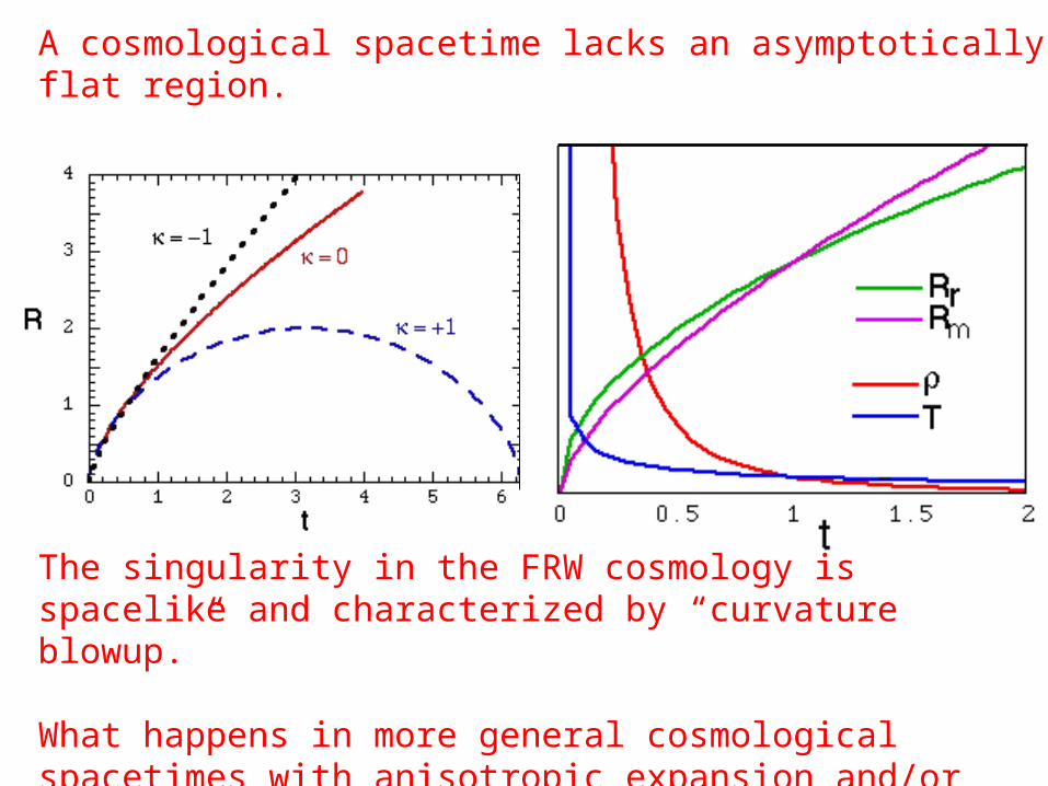
A cosmological spacetime lacks an asymptotically flat region.

The singularity in the FRW cosmology is spacelike and characterized by “curvature blowup.”

What happens in more general cosmological spacetimes with anisotropic expansion and/or spatial inhomogeneities?

Cosmological spacetimes can have anisotropic expansion and no matter:

Anisotropy “energy” can act as a source for expansion. Spatial scalar curvature V will act as a “potential” for the dynamics in “minisuperspace.”

Hubble parameter

Curvature potential

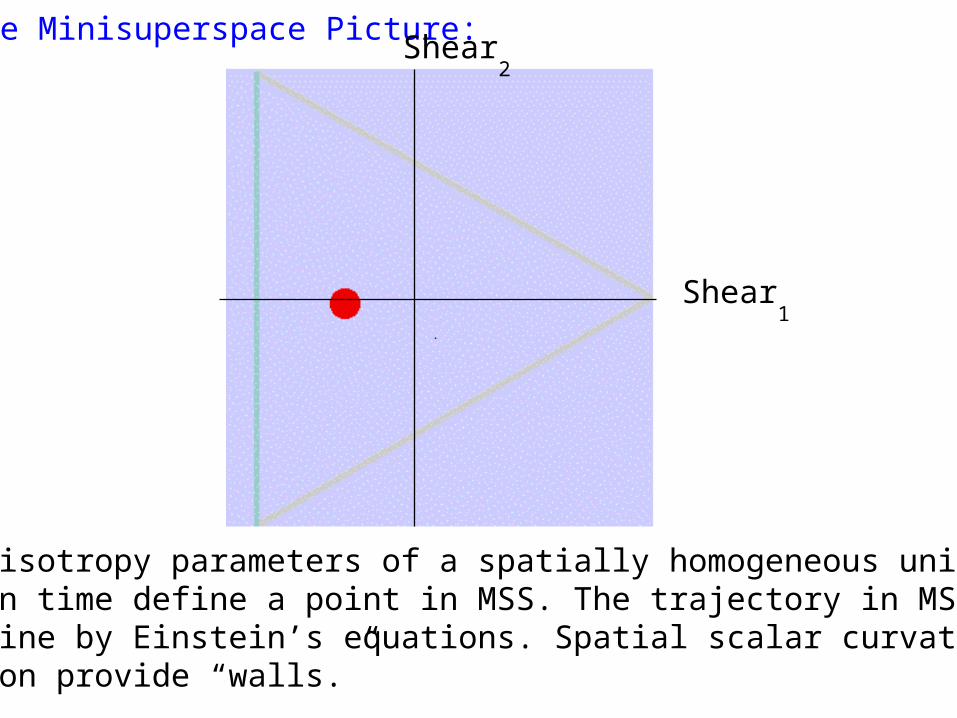
The Minisuperspace Picture:

The anisotropy parameters of a spatially homogeneous universe at a given time define a point in MSS. The trajectory in MSS isdetermine by Einstein’s equations. Spatial scalar curvature androtation provide “walls.”

Shear1

Shear2

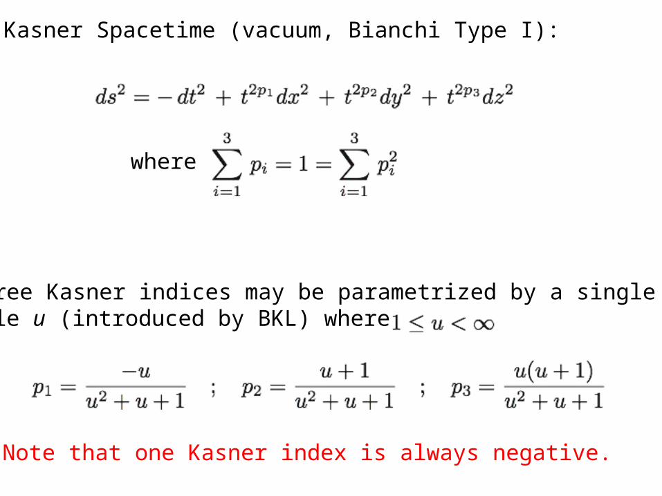
The Kasner Spacetime (vacuum, Bianchi Type I):

where

The three Kasner indices may be parametrized by a single variable u (introduced by BKL) where :

Note that one Kasner index is always negative.

The Kasner Spacetime (vacuum, Bianchi Type I):

1 10 100

u

0

1

2/3

-1/3

p3

p2

p1

Each u-value in indicates a distinct Kasner evolution.

A set of measure zero: The (1,0,0) Kasner is the Minkowski spacetime in different coordinates. “Milne universe”

The Kasner Singularity:

In the collapse (expansion) direction, one Kasner axis is expanding (collapsing). However,

and the first non-zero curvature invariant blows up asunless :

This is a spacelike, curvature blowup singularity just as for FRW.

The Kasner Spacetime is a “free particle” in minisuperspace:

In terms of and the momenta conjugate to the MSS variables, Einstein’s equations may be obtained by variation of the Hamiltonian constraint

to yield

Note that the straight line trajectory in MSS may be described by a single angle θ which may be shown to be equivalent to u.

The Kasner singularity is “velocity term dominated” (VTD).

“Kasner circle.”

Aside on the role of matter (or effective matter):

0

0.5

1

1.5

0

0.2

0.4

0.6

0.8

1

0 0.2 0.4 0.6 0.8 1

DeSitterKasnerKasner + Λ

( / )log shear expansion

( )a t

Anisotropy

t

Taub spacetime (vacuum Bianchi Type II):

For these models, the Hamiltonian constraint

may be solved to yield

This can be treated exactly as scattering off an exponential potential relating the initial Kasner epoch to the final Kasner epoch.

This singularity is “asymptotically velocity term dominated” (AVTD) because there is a last “bounce” off the potential.

Conservation of momentum can be used to develop “bounce laws”to relate asymptotically constant variables before (e.g. ) and after (e.g. ) the bounce off the potential:

V(w)

w

E

-1

-0.5

0

0.5

1

-1 -0.5 0 0.5 1

β−/|Ω|

β+/|Ω|

Typical trajectory in minisuperspace:

(The single “wall” could be oriented at any angle.)

Method of Consistent Potentials (Grubisic, Moncrief) :

1. Neglect all terms arising from spatial dependence

and solve the truncated Einstein equations (ODE's).

This yields the Velocity Term Dominated solution

as τ → ∞ .at each spatial point

2. Substitute the VTD solution into the full Einstein

.equations If all previously neglected terms are

exponentially small as τ → ∞, we predict that the full

solution is Asymptotically VTD .

3. Terms which are not exponentially small act as

.potentials which then dominate the dynamics

4. Compare the prediction to numerical simulations

.of the full Einstein equations

Note that spatial scalar curvature in spatially homogeneous cosmologies arises from spatial derivatives.

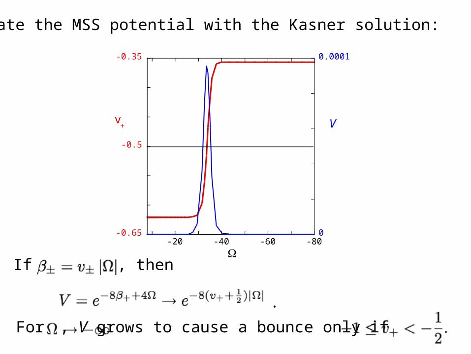
Evaluate the MSS potential with the Kasner solution:

-0.65

-0.5

-0.35

0

0.0001

-80-60-40-20

v+ V

ΩIf , then

For , V grows to cause a bounce only if

.

The “most general” homogeneous cosmology is (non-diagonal) Bianchi IX:

• Mixmaster models (diagonal)

where

In minisuperspace,

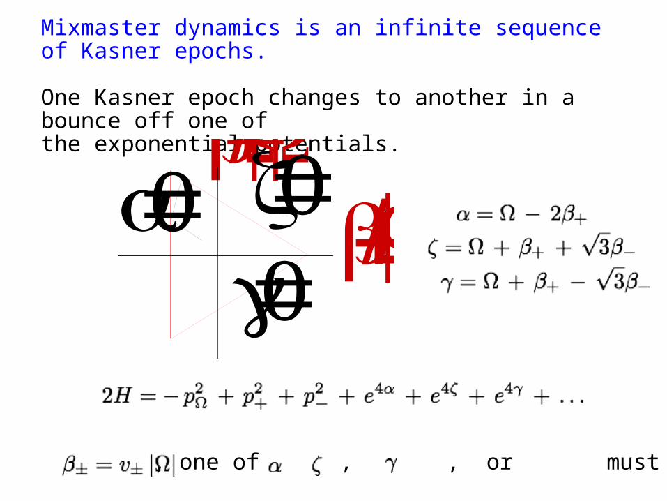
If , one of , , or must grow.

Mixmaster dynamics is an infinite sequence of Kasner epochs.

One Kasner epoch changes to another in a bounce off one of the exponential potentials.

β+/|Ω|β−/|Ω|

α = 0 ζ = 0γ = 0

-80

-40

0

-24

-12

0

0 100 200 300 400 500 600

β

+

V

α

V

ζ

V

γ

β

+

log

10

V

| Ω|

From a numerical simulation:

B e r g e r , B . K . , G a r Ø n k l e , D . , a n d S t r a s s e r , E . , C l a s s . Q u a n t u m G r a v . 1 4 , L 2 9 ( 1 9 9 6 ) .GarfinkleBKB, D. Garfinkle, E. Strasser, CQG 14, L29 (1996).

0

1

2

3

4

5

6

7

8

2000 3000 4000 5000 6000 7000 8000

u

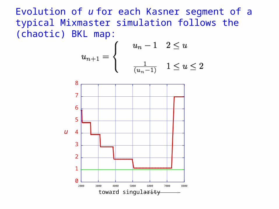
toward singularity

Evolution of u for each Kasner segment of a typical Mixmaster simulation follows the (chaotic) BKL map:

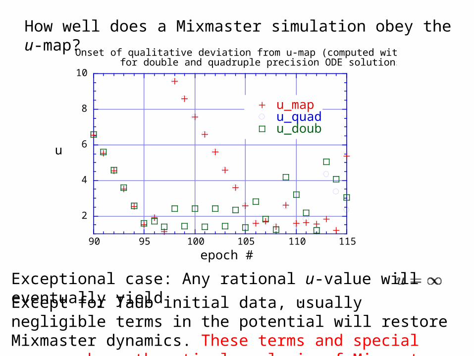
How well does a Mixmaster simulation obey the u-map?

2

4

6

8

10

90 95 100 105 110 115

Onset of qualitative deviation from u-map (computed with Mathematica) for double and quadruple precision ODE solutions.

u_mapu_quadu_doub

u

epoch #

Exceptional case: Any rational u-value will eventually yield .

Except for Taub initial data, usually negligible terms in the potential will restore Mixmaster dynamics. These terms and special cases make mathematical analysis of Mixmaster dynamics difficult.

A Mixmaster simulation with > 250 bounces:

Ringström has proven that the Mixmaster singularity for non-Taub initial data is of the curvature blow-up type.

H. Ringström, Class.Quant.Grav. 17 (2000) 713-731.

Ω is a logarithmic time coordinate. The ratio of the Planck time to the Hubble time gives ΔΩ ≈ 1000. However, 250 bounces requires ΔΩ ≈ 1060 .

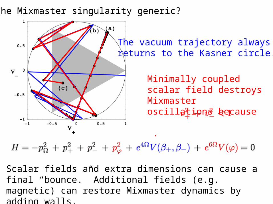
Minimally coupled scalar field destroys Mixmaster oscillations because .

Is the Mixmaster singularity generic?

Scalar fields and extra dimensions can cause a final “bounce.” Additional fields (e.g. magnetic) can restore Mixmaster dynamics by adding walls.

The vacuum trajectory alwaysreturns to the Kasner circle.

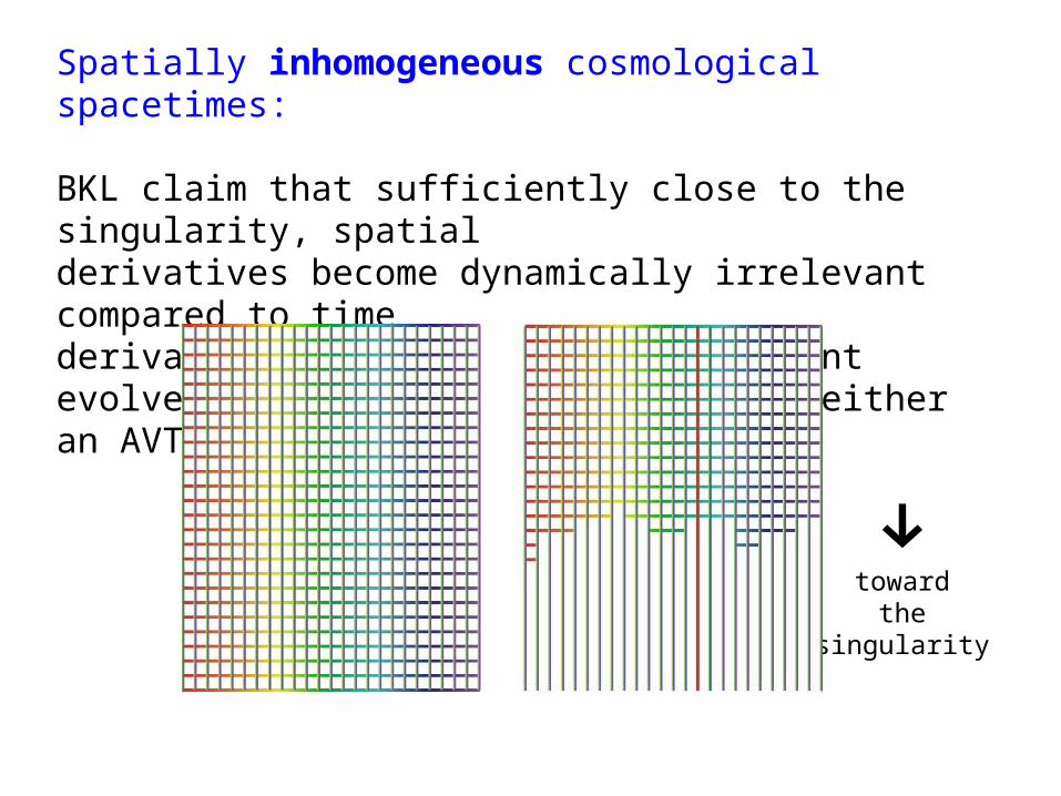
Spatially inhomogeneous cosmological spacetimes:

BKL claim that sufficiently close to the singularity, spatialderivatives become dynamically irrelevant compared to timederivatives so that each spatial point evolves as a separate universe with either an AVTD or Mixmaster singularity.

↓toward

thesingularity

A synergy between mathematics and simulations has yieldedimproved understanding of singularities in general relativity. How does this synergy work?

Mathematics:

+ Statements may be made about large classes of solutions.

– Properties of explicit solutions may remain unknown.

Numerical simulations:

+ Explicit solutions may be found for complicated nonlinear equations.

– Only 1 solution may be studied at a time. Exploration of parameter space may be necessary.

Mathematical and numerical singularity studies of inhomogenous cosmologies

• Polarized Gowdy is AVTD: Isenberg & Moncrief

• Gowdy is AVTD: Berger & Moncrief, Berger & Garfinkle, Kichenassamy & Rendall

• Polarized twisted Gowdy is AVTD: Isenberg & Kichenassamy

• Magnetic Gowdy is locally Mixmaster dynamics: Weaver, Isenberg, & Berger

• Twisted Gowdy is locally oscillatory: Weaver, Isenberg, & Berger

• Polarized U(1) is AVTD: Berger & Moncrief, Isenberg & Moncrief

• U(1) is locally oscillatory: Berger & Moncrief

• U(1) + scalar field is AVTD: Berger

• Generic + scalar field is AVTD: Andersson & Rendall, Garfinkle

• Generic is locally Mixmaster: Garfinkle

Math: Prove that open set of solutions with conjectured properties exists. (Fuchsian methods allow construction of solution starting at singularity.)

θ

“Quantitative” studies of T2 symmetric spatially

inhomogeneous cosmologies with T3 spatial topology:

x

y

Polarized Gowdy: spatial axes are fixedGeneric Gowdy: orientation of x and y axes changes with time

General T2 symmetric: orientation of all spatial axes depends on time

Gowdy models are both an arena for precision numerics and mathematically tractable creating a valuable synergy:

Einstein’s equations consist of wave equations for P and Q and constraints which may be solved for λ The wave equationsmay be obtained by variation of

where .

As , the VTD solution (neglect spatialderivatives) is

Terms in the Hamiltonian act as potentials. For AVTD behavior of the model, these potentials must decay exponentially.

requires for consistency.

requires for consistency.

This means that the singularity is AVTD (at any spatial point) only if .

Competing Potentials in Equation for P

V

2

= e

2 ( P − τ )

Q ,

θ

2

V

2

( )Z

= - Z P τ

( P ,

τ

− 1 )

2

V

1

= e

− 2 P

π

Q

2

P

V

1

( )P

P ,τ

2

Gowdy wαλλs αs Mixmαsτer MSS

-4

-2

0

2

-3

-2

-1

0

1

0 2 4 6 8 10

P

V1

V2

Plog

10V

τ

Numerical simulations show how v is driven intothe range (0,1) by bounces off the potentials. A typical single spatial point is shown.

B.K. Berger, D. Garfinkle, Phys. Rev. D 57, 4767 (1998).

Numerical simulations show how is driven into the range (0,1)by bounces off the potentials. A typical single spatial point is shown.

P

θ

Q

θ

0

2

4

6

8

3.10 3.14 3.18

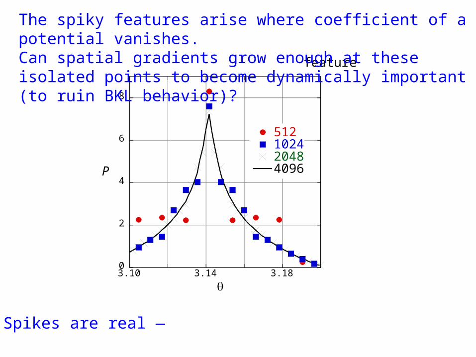
Not quite resolved feature

512102420484096P

θ

The spiky features arise where coefficient of a potential vanishes. Can spatial gradients grow enough at these isolated points to become dynamically important (to ruin BKL behavior)?

Spikes are real —

A.D. Rendall, M. Weaver, “Manufacture of Gowdy Spacetimes with Spikes,”CQG 18, 2959 (2001)

— but are understood mathematically:

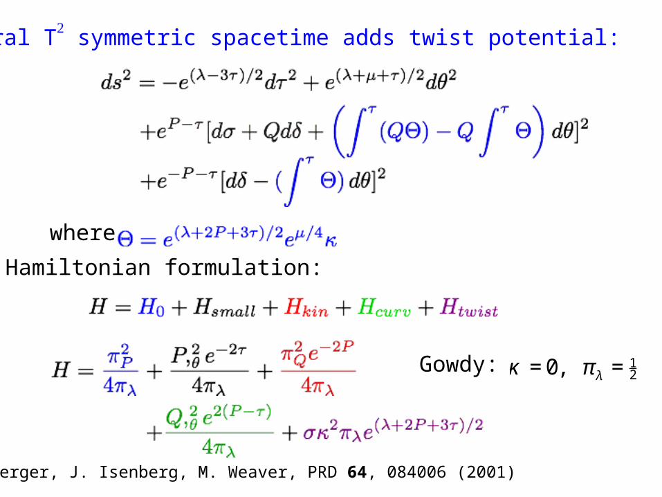
General T2 symmetric spacetime adds twist potential:

where

Hamiltonian formulation:

B.K. Berger, J. Isenberg, M. Weaver, PRD 64, 084006 (2001)

Gowdy: κ =0, πλ =12

H = HK

+ HC

+ HM

=

1

4 πλ

πP

2

+ e− 2 P

πQ

2

( )

+

1

4 πλ

e− 2 τ

P ,θ

2

+ e2 ( P − τ )

Q ,θ

2

( )

( λ + 2 P + 3 τ ) / 2

πλ

e+

Twisτed Gowdy ( , ):with Isenberg Weaver

K2

G

τwisτ πoτenτiαλ

TwistedGowdy walls as Mixmaster

MSS

Twist potential causes local Mixmaster dynamics:

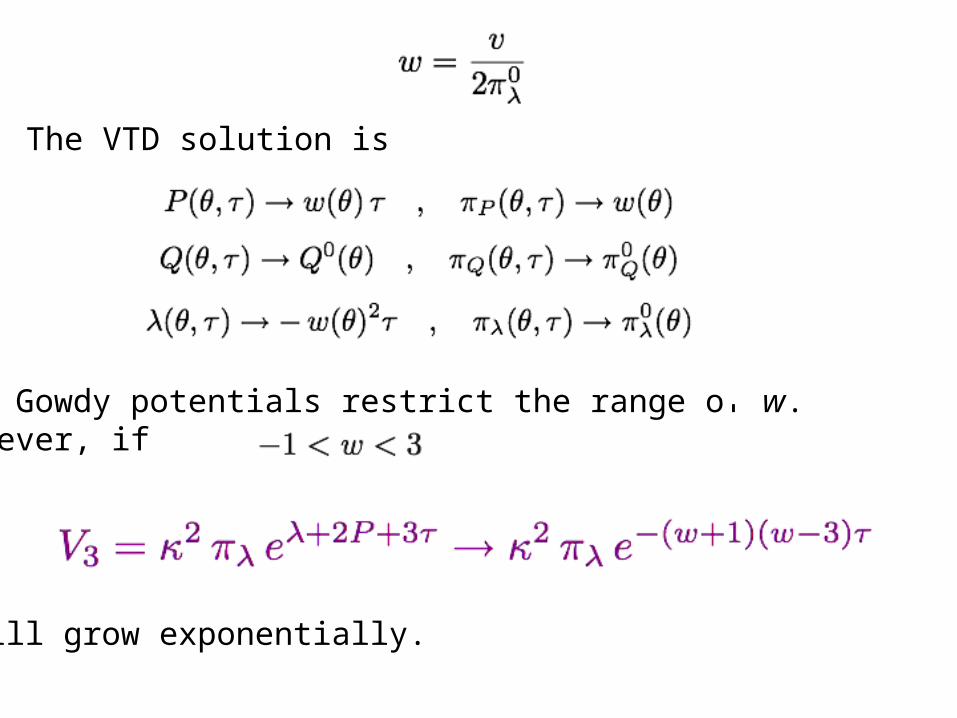
The Gowdy potentials restrict the range of w. However, if

The VTD solution is

will grow exponentially.

P

P

θ

θ

-10

0

10

20

30

40

50

0 10 20 30 40 50 60 70 80

w

τ

Behavior at 3 typical points (offset for clarity)

Bounce laws relate w before and after bounce. Quantitative agreement is found.

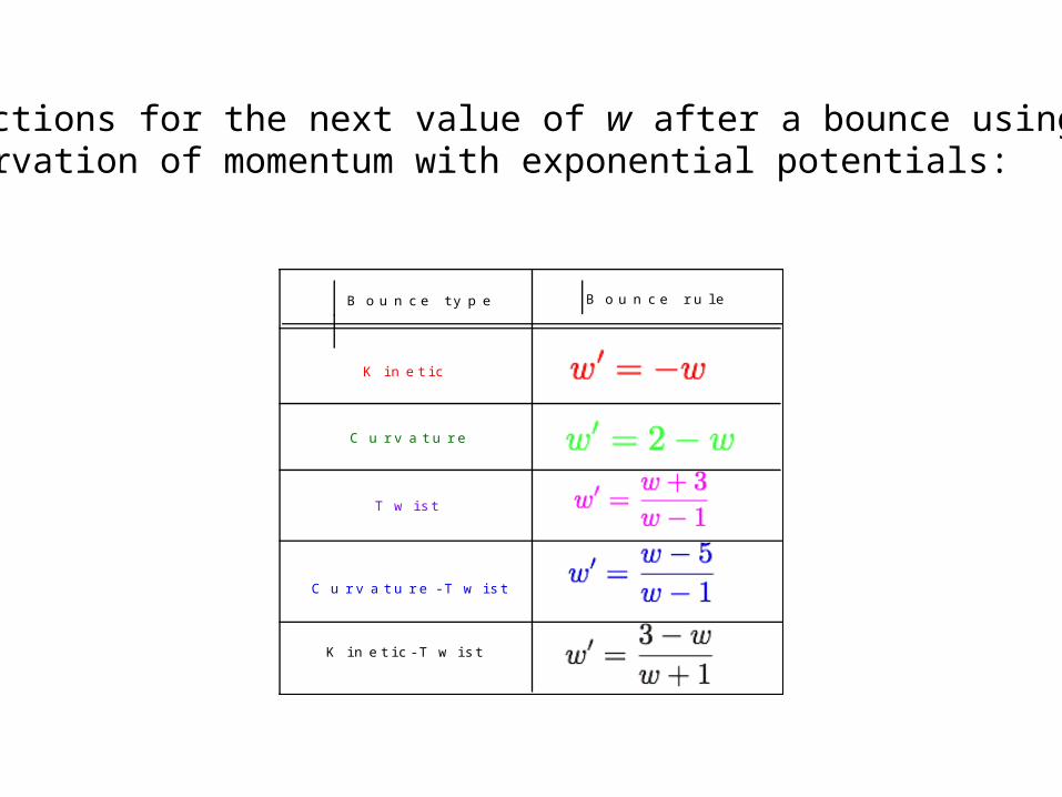
Predictions for the next value of w after a bounce usingconservation of momentum with exponential potentials:

w0

= 2 ° w

B o u n c e t y p e

K i n e t i c

C u r v a t u r e

T w i s t

C u r v a t u r e - T w i s t

K i n e t i c - T w i s t

B o u n c e r u l e

w0

= ° w

w0

=w + 3

w ° 1

w0

=w ° 5

w ° 1

w0

=3 ° w

w + 1

–

–

–

––

–

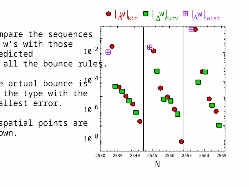
10-8

10-6

10-4

10-2

2530 2535 2540 2545 2550 2555 2560 2565

|Δw|kin

| Δw|curv

|Δw|twist

N

Compare the sequencesof w’s with those predictedby all the bounce rules.

The actual bounce is of the type with the smallest error.

3 spatial points areshown.

10-6

10-4

10-2

100

0 1000 2000 3000 4000 5000

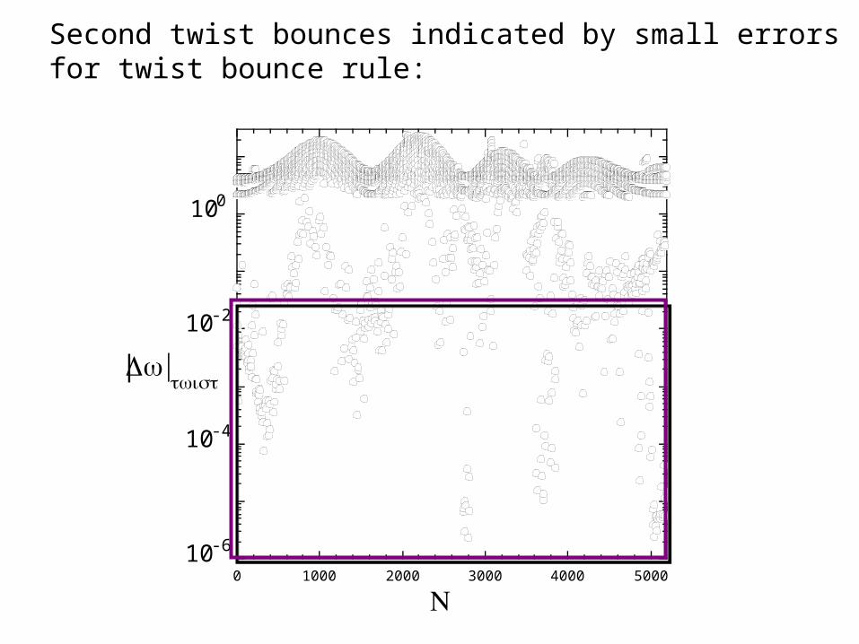
|Δw|twist

N

Second twist bounces indicated by small errors for twist bounce rule:

No spatial symmetries (Garfinkle): Add scalar field to suppress Mixmaster oscillations.

D. Garfinkle, PRD 65, 044029 (2002)

L. Andersson, A.D. Rendall, Comm. Math. Phys. 218, 479 (2001)

0

1

2

3

4

5

6

7

8

2000 3000 4000 5000 6000 7000 8000

u

toward singularity

Evolution of u from a typical Mixmaster simulation.

REMINDER

No spatial symmetries (Garfinkle): (vacuum case)

D. Garfinkle, Phys.Rev.Lett. 93 (2004) 161101

Toward the singularity

Behavior of u at a typical spatial point:

Mathematical results exist only for AVTD models.

-1

0

1

-1 0 1

p− / |p

Ω|

p+ / |p

Ω|

-1

0

1

-1 0 1

β− / |Ω|

β+ / |Ω|

Uggla et al, Phys.Rev. D68 (2003) 103502, Heinzle et al arXiv:gr-qc/0702141, T. Damour, S. de Buyl, arXiv:0710.5692;Henneaux et al., arXiv:0710.1818.

See C. Uggla, arXiv:0706:0463 [gr-qc] for most recent status.

Development of (complementary) frameworks to “prove” BKL conjecture:

Set up Iwasawa variables at each point and understand the spatial properties and bounces.

Rescaled variables allow focus on the Kasner circle as an attractor for dynamical systems of PDEs.

No proof yet!

P.R. Brady, J.D. Smith, Phys. Rev. Lett. 75, 1256 (1995).

Analytic and numerical evidence indicates that the singularity inside a Riessner-Nordstrom or Kerr black hole is first seen to be null and weak. (An infalling observer would not experience infinite tidal forces.) Many infalling observer world lines end at the null singularity. It eventually becomes spacelike and strong.

L.M. Burko, Phys. Rev. D 59, 024011 (1999).

Comment on singularities inside black holes:

P

θ

P

θ

S

2

× S

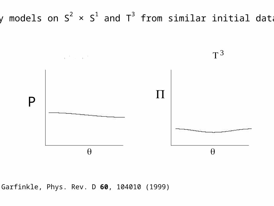
1 T 3

Gowdy models on S2 × S

1 and T

3 from similar initial data;

D. Garfinkle, Phys. Rev. D 60, 104010 (1999)

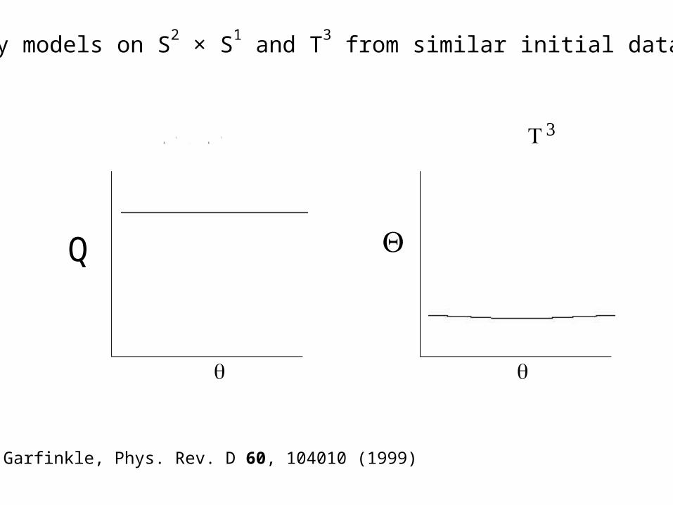
Q

θ

Q

θ

S

2

× S

1 T 3

Gowdy models on S2 × S

1 and T

3 from similar initial data;

D. Garfinkle, Phys. Rev. D 60, 104010 (1999)

-4

-2

0

2

4

6

8

10

0

20

40

60

80

100

120

0 4 8 12 16 20 24 28 32

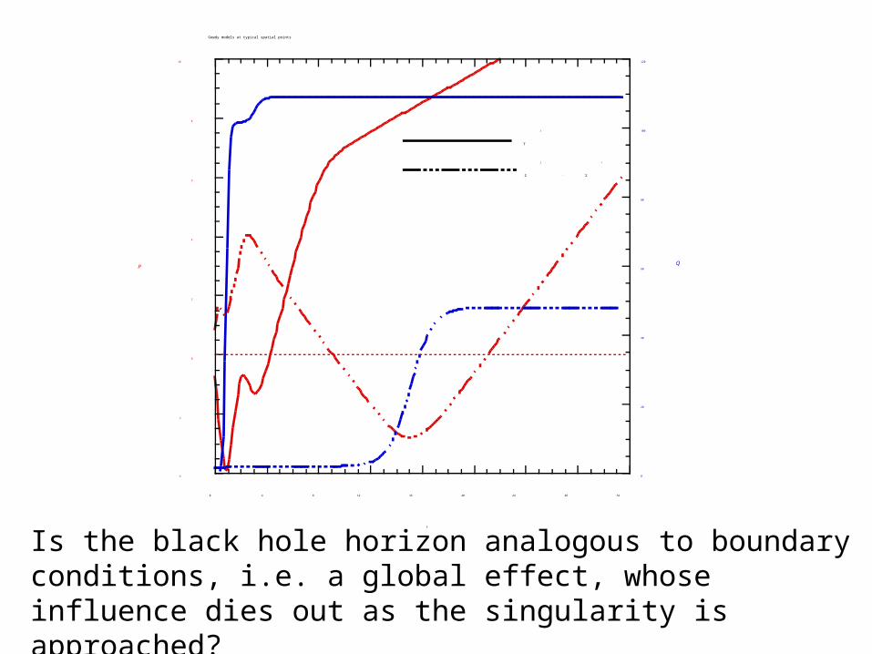
Gowdy models at typical spatial points

PQ

τ

T

3

S

2

× S

1

Is the black hole horizon analogous to boundary conditions, i.e. a global effect, whose influence dies out as the singularity is approached?

Conclusions

• There is strong evidence from numerical simulation (and also mathematical theorems) that generic collapse leads to spacelike singularities dominated by local dynamics.

• Asymptotically, the local behavior closely follows the Kasner or Mixmaster solution.