geo372 vertiefung giscience data quality and integrationgeo372 vertiefung giscience data quality and...
TRANSCRIPT

Geo372Vertiefung GIScience
Data quality and integration
Herbstsemester
Ross Purves
These slides use some materials originally prepared by R. Weibel
Outline
Two part lecture exploring and relating data quality and integration
• What is spatial data quality and why should we care?
• How can we usefully define and describe data quality?
• How can spatial data be integrated using location?
• What issues can arise and how do these relate to data quality?

Learning objectives
You will be able to:
• give examples of how uncertainty in spatial data quality can lead to unexpected consequences;
• define accuracy, error, precision and resolution with examples;
• for a given data set, with suitable additional information, you can populate the “Famous Five” of the Spatial Data Transfer Standard;
• describe the process of data integration is in terms of vector and raster data;
• be able to list some of the common problems with polygon overlay, and suggest techniques to minimise these; and
• describe applications of data integration and the influence of data quality.

What is spatial data quality?• Quality can mean different things:
⁻ “Schweizer Qualität” - Best possible result, with no regard to cost and time?
⁻ Passing some threshold specified by a customer or national/ international standards
⁻ “Fitness for use” — in terms of a defined application
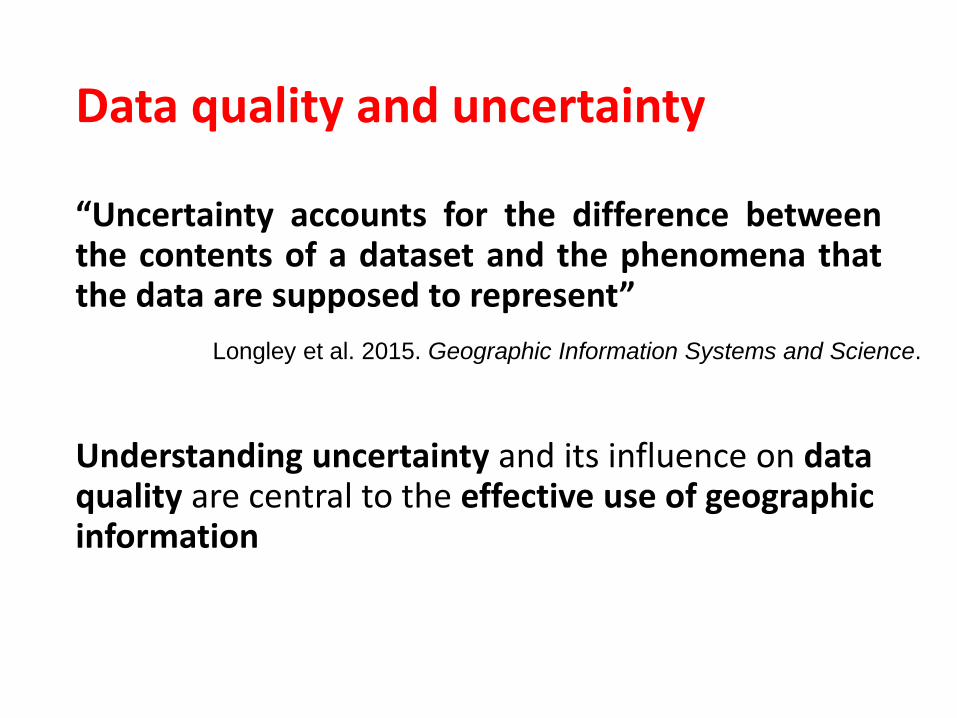
Data quality and uncertainty
“Uncertainty accounts for the difference betweenthe contents of a dataset and the phenomena thatthe data are supposed to represent”
Understanding uncertainty and its influence on data quality are central to the effective use of geographic information
Longley et al. 2015. Geographic Information Systems and Science.

Conceptual view of uncertainty sources
At each of these stages
uncertainty can be
introduced which should be
reported with respect to the
data quality and may
have an influence on the
data’s fitness for use
Real world
Concepts
Measurement and representation
Analysis
Figure after Longley et al. 2015. Geographic Information Systems and Science.
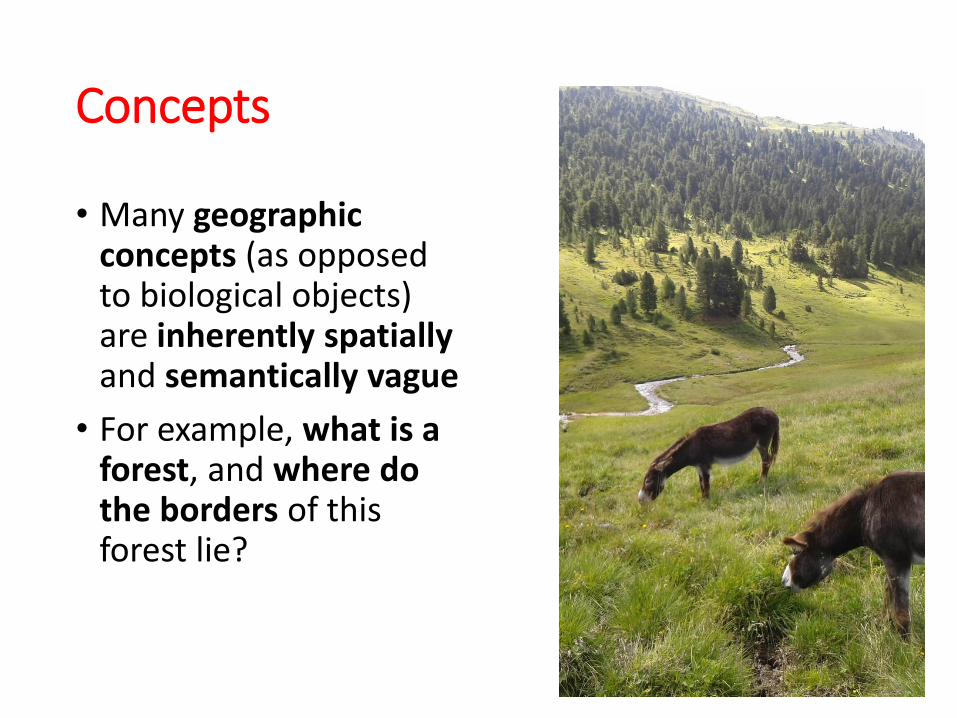
Concepts
• Many geographic concepts (as opposed to biological objects) are inherently spatially and semantically vague
• For example, what is a forest, and where do the borders of this forest lie?

Example: Change bog definition?
• 1990 Land Cover Map of Great Britain (~Arealstatistik) defined bog as “standing water, permanent water logging, surface water and characteristic plant species”
• 2000 Land Cover Map of Great Britain defined bog as peat depth deeper than 50cm
• Bog in one 100x100km1 tile changed from <1 ha to ~75km2!
• Does it matter – bog is an important carbon sink –but all this change is to do with definition not in the real world…
1Resolution 25mExample from Comber et al., 2006.

Measurement
• “The grounding occurred when the jack-up barge Octopus, with a draught of 13m, grounded on an uncharted 7.1m shoal. The charted depth at the grounding position, based on a 19th Century leadlinesurvey, was 26m.”
• Damage cost 1 million pounds to repair…
Source (www.maib.gov.uk/cms_resources/Harold_Octopus.pdf)
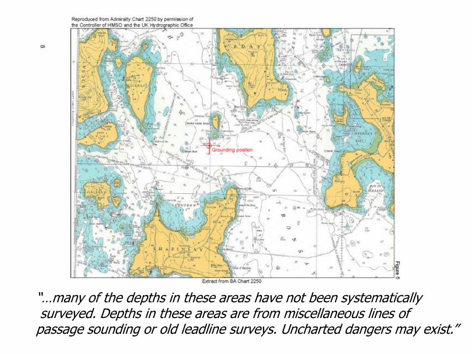
“…many of the depths in these areas have not been systematicallysurveyed. Depths in these areas are from miscellaneous lines of passage sounding or old leadline surveys. Uncharted dangers may exist.”

From: http://celebrating200years.noaa.gov/breakthroughs/hydro_survey/lead_lini
ng_650.html
From:http://www.maib.gov.uk/cms_resources/Harold_Octopus.pdf
The charts used have not been resurveyed since ~1843 and are based on lead-line data –reef not found in original survey
Note original data contain no contours (points are not interpolated)

Representation
How we represent concepts also has an influence on uncertainty – neither of these representations is per se wrong
Zermatt and surroundings in rasters with 100m and 20km resolution

Source: THE ECONOMIST (2003), North Korea's Missile Threat
Analysis
Poorly chosen analysis methods can introduce uncertainty, even in simple (but important!) calculations

Can’t we just work with perfect data?
• Perfect data cannot exist – all representations have associated uncertainties
• We need to understand uncertainty to make sure that our application of spatial data is fit for purpose
• The best way to do this is to document and understand the influence of uncertainty and clearly define the purpose of an analysis
• We’ll start doing this with a few definitions…

Definitions (1)
• Accuracy – the difference between a recorded value and its true value (often divided into spatial, topological and attribute accuracy). In practice truth is also a measured reference value, which is assumed to be more accurate
• Error – describes the deviation of a value from truth: often characterised as:• Blunders (gross errors)
• Systematic errors (bias)
• Random errors
After Jones, 1997. Geographical Information Systems and Computer Cartography (Chapter 7)

Definitions (2)
• Precision – the detail with which a measurement is reported – there is no point reporting a measurement to a higher precision than that with which it is measured
• Resolution – smallest distance/ time /theme over which change is measurable (often a synonym for precision)
• All of these definitions can be applied to both nominal/ ordinal and numerical measurements
After Jones, 1997. Geographical Information Systems and Computer Cartography (Chapter 7)
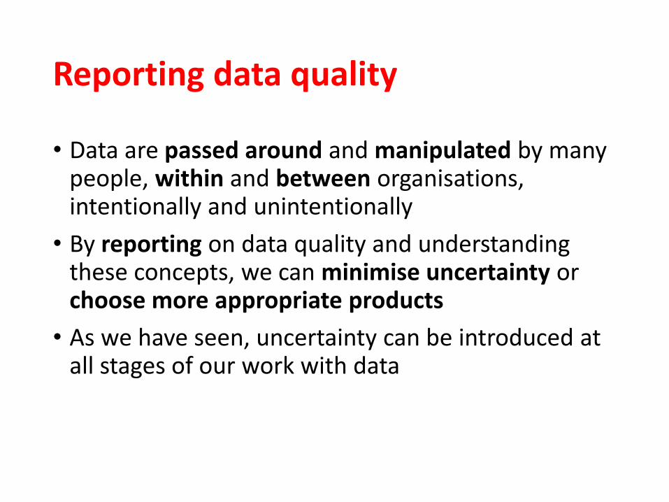
Reporting data quality
• Data are passed around and manipulated by many people, within and between organisations, intentionally and unintentionally
• By reporting on data quality and understanding these concepts, we can minimise uncertainty or choose more appropriate products
• As we have seen, uncertainty can be introduced at all stages of our work with data

Zooming in on the SDTS1
• Developed in the US to allow transfer of data between organisations using a defined and agreed standard
• It is obligatory for US Federal Organisations to use the SDTS
• Includes compulsory data quality fields – you can think about how these map to the conceptual view of uncertainty sources
1Spatial Data Transfer Standard
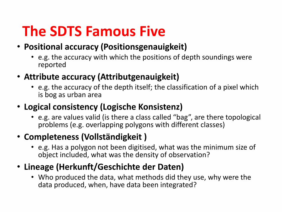
The SDTS Famous Five• Positional accuracy (Positionsgenauigkeit)
• e.g. the accuracy with which the positions of depth soundings were reported
• Attribute accuracy (Attributgenauigkeit)• e.g. the accuracy of the depth itself; the classification of a pixel which
is bog as urban area
• Logical consistency (Logische Konsistenz)• e.g. are values valid (is there a class called “bag”, are there topological
problems (e.g. overlapping polygons with different classes)
• Completeness (Vollständigkeit )• e.g. Has a polygon not been digitised, what was the minimum size of
object included, what was the density of observation?
• Lineage (Herkunft/Geschichte der Daten)• Who produced the data, what methods did they use, why were the
data produced, when, have data been integrated?

Summing up so far
• We defined data quality – most important is that our data is fit for use
• We saw three examples where data were clearly not fit for a particular use (and one where a misunderstanding meant that the resulting product was simply wrong)
• We looked at some important definitions of terms related to spatial data quality and uncertainty
• We explored how we can report on spatial data quality
Integrating spatial data
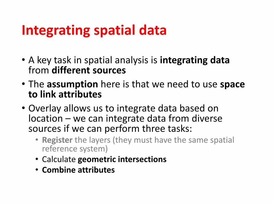
• A key task in spatial analysis is integrating data from different sources
• The assumption here is that we need to use space to link attributes
• Overlay allows us to integrate data based on location – we can integrate data from diverse sources if we can perform three tasks:• Register the layers (they must have the same spatial
reference system)• Calculate geometric intersections • Combine attributes
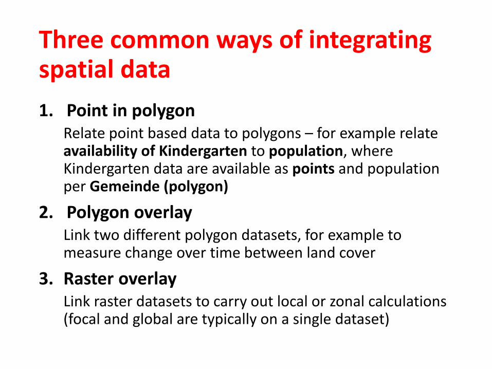
Three common ways of integrating spatial data
1. Point in polygonRelate point based data to polygons – for example relate availability of Kindergarten to population, where Kindergarten data are available as points and population per Gemeinde (polygon)
2. Polygon overlayLink two different polygon datasets, for example to measure change over time between land cover
3. Raster overlayLink raster datasets to carry out local or zonal calculations (focal and global are typically on a single dataset)

Point in polygon
• Computationally straightforward
• Point and polygon granularity can be important
• Planar enforcement* of polygons matters
• Boundary special cases need to be understood
Basic algorithm: point lies in a
polygon when a semi-infinite ray
has an odd number of intersections
*Space filled, no overlapping polygons
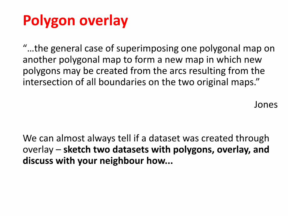
Polygon overlay
“…the general case of superimposing one polygonal map onanother polygonal map to form a new map in which newpolygons may be created from the arcs resulting from theintersection of all boundaries on the two original maps.”
Jones
We can almost always tell if a dataset was created throughoverlay – sketch two datasets with polygons, overlay, anddiscuss with your neighbour how...

How does polygon overlay work?• Polygon overlay is computationally complex –
developing efficient algorithms was a major issue for vector GIS
• In polygon overlay we must• Calculate intersections between polygons on different
layers and create new polygons• Build an attribute table representing all the attributes of
each of our new polygons (each new polygon can have attributes for every layer)
• According to the calculation being carried out label a new set of polygons (and if adjacent polygons share attribute values dissolve boundaries)
• Deal with errors in the process (sliver polygons)
• The exact process depends on whether our data has a topology

Problems with polygon overlay• Most problems with polygon overlay are because the
accuracy of our digitised lines is not comparable to the precision of our representation
• Furthermore, different layers may record a feature which is coincident in space but are not stored in different datasets with exactly equivalent positions
• This may be because datasets were generated at different scales, by different people, at different times or through different processes –back to data quality

Slivers• When different layers have a high spatial correlation between
polygon boundaries, overlay can result in sliver polygons
• Slivers are small, spurious polygons which result as part of the overlay process
• They tend to occur when the same features occur as polygon boundaries in several layers (for example rivers or district boundaries) or where the same feature is multiply digitisedover time (e.g. land use borders) or at the edge of a map sheet
Local boundary follows river
Digitised river (from different source)
Overlay results in
spurious sliver
polygons

Dealing with slivers…
There are two techniques we can use:
• During overlay – techniques attempt to snap adjacent arcs/ nodes together to prevent sliver formation (you’ve been doing this)… • use techniques based on fuzzy tolerances – if a node or arc is
within some predetermined distance then snap them together
• Tends to smooth lines and may remove detail as well as slivers
• Post overlay – techniques attempt to identify and remove slivers (you’ll do this in the practical)
• What geometric properties will drive the number and area of sliver polygons?
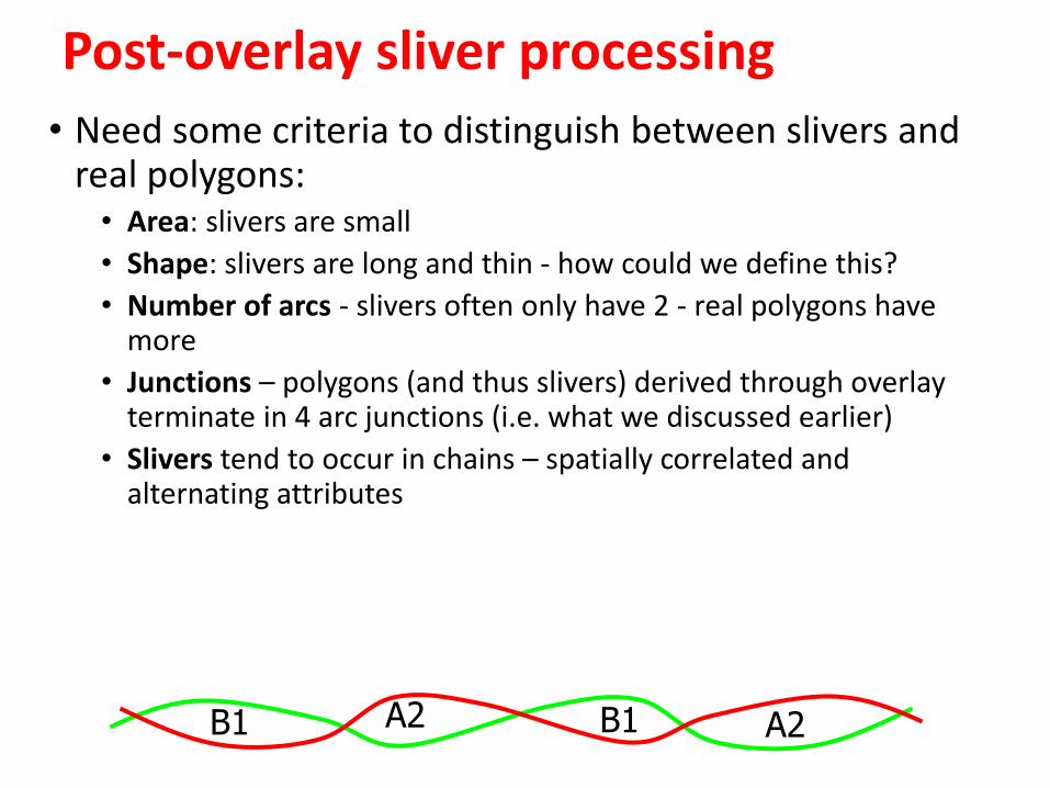
Post-overlay sliver processing
• Need some criteria to distinguish between slivers and real polygons:• Area: slivers are small
• Shape: slivers are long and thin - how could we define this?
• Number of arcs - slivers often only have 2 - real polygons have more
• Junctions – polygons (and thus slivers) derived through overlay terminate in 4 arc junctions (i.e. what we discussed earlier)
• Slivers tend to occur in chains – spatially correlated and alternating attributes
B1 A2 B1 A2

Polygon overlay in spatial analysis
• Now we know how polygon overlay works – what can we use it for…
• We can use overlay to ask questions and describe our datasets
• Many simple operations use overlay, without us even noticing
• The following is a list of overlay operations, as implemented in ArcGIS
• Note that the names of the operations may vary between GIS (and not all operations are possible in all GIS)

Polygon overlay in ArcMap
Input
features
Overlay
features
Result
Identity
Intersect
Symmetrical
difference
Union
Update
From: http://desktop.arcgis.com/en/arcmap/latest/analyze/commonly-used-tools/overlay-analysis.htm

Raster overlay
• Raster overlay is computationally simple
• Registration is the biggest problem: all rasters must have the same resolution (not always a sensible assumption) and projection
• If this is the case, then combining attributes from multiple rasters is straightforward
A
B
C
U=f(A,B,C)

Using overlay for analysis

Lead in Flint• You read (I hope) the blog
post I sent you
• I had three questions for you:
• What question was being asked of the data (what was the hypothesis being tested?)
• What data (and how) were collected?
• How were the data analysed?
Interpolated map of blood lead levels based on geocode addresses (more on interpolation next week)
Source: Hanna-Attisha et al. (2016). Elevated blood lead levels in children associated with the Flint drinking water crisis: a spatial analysis of risk and public health response. AJPH, 106(2), 283-290.

Change detection
• Change detection is one of the most important, and “simplest” uses of overlay
• Imagine we wish to see how a town has grown
• If we simply have the boundaries of the urban area at different times we can compare the original area with the new area through time
• At each time step we can measure how much change there has been
• A key question is how much change is real and how much results from uncertainty
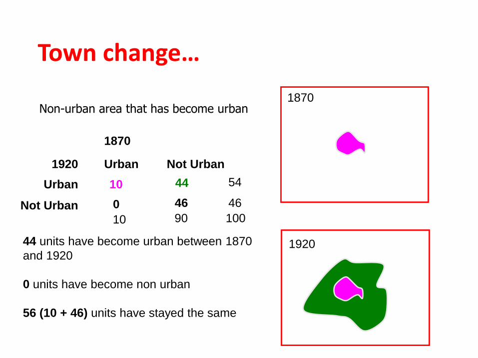
Town change…
Non-urban area that has become urban
Urban
Not Urban
Urban
Not Urban
1870
1920
10 44
0 46
44 units have become urban between 1870
and 1920
0 units have become non urban
56 (10 + 46) units have stayed the same
54
46
10 90 100
1870
1920

Land cover maps of Orango for 1956 (top) and 1998 (bottom).
Vasconcelos et. al. 2002. Land cover change in two protected areas of Guinea-Bisseau.Applied Geography, 22, 139-156.
Using overlay to detect land cover change on a small island of the west coast of Africa
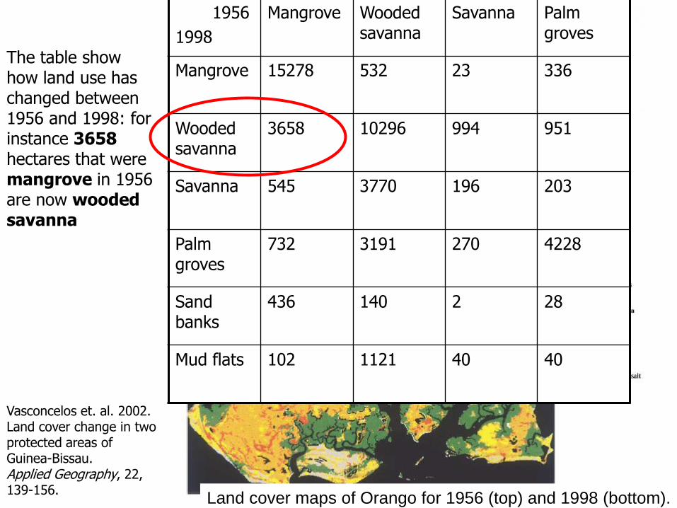
Land cover maps of Orango for 1956 (top) and 1998 (bottom).
The table showhow land use haschanged between1956 and 1998: forinstance 3658 hectares that were mangrove in 1956are now wooded savanna
Vasconcelos et. al. 2002. Land cover change in two protected areas of Guinea-Bissau.Applied Geography, 22, 139-156.
1956
1998
Mangrove Wooded savanna
Savanna Palm groves
Mangrove 15278 532 23 336
Wooded savanna
3658 10296 994 951
Savanna 545 3770 196 203
Palm groves
732 3191 270 4228
Sand banks
436 140 2 28
Mud flats 102 1121 40 40
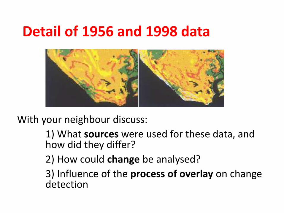
Detail of 1956 and 1998 data
With your neighbour discuss:
1) What sources were used for these data, and how did they differ?
2) How could change be analysed?
3) Influence of the process of overlay on change detection
Summary
• We’ve explored data integration – there are many ways of integrating spatial data based on locations
• We looked at:• Point in polygon• Polygon overlay• Raster overlay
• Data quality is of central importance in understanding the results of data integration
• Fitness for use depends on the questions being asked• In our point in polygon operation unsuitable spatial units led to
misleading results (Modifiable Area Unit Problem)• In today’s practical you will overlay two polygon datasets to
explore change: you should think about the whole uncertainty chain (concepts; measurement and representation; analysis)
• Change detection focuses on comparing datasets which are temporally different, but spatially coherent – but as our examples showed, definitions and collection methods also change
Next week
• We will look at spatial interpolation
• How can we use values that are sampled at discrete points in space to estimate a value anywhere within some extent?
• Why can’t we just use inverse-distance weighting all the time (refresh your memories about IDW)
• How can we compare and assess the quality of different interpolators for different problems?
References• Burrough, P.A. et al. (2015): Principles of Geographical
Information Systems. Third Edition. Oxford University Press.
• Comber et al. (2006): Using metadata to link uncertainty and data quality assessments. In Progress in Spatial Data Handling (12th International Symposium on Spatial Data Handling). Springer
• Hanna-Attisha et al. (2016). Elevated blood lead levels in children associated with the Flint drinking water crisis: a spatial analysis of risk and public health response. AJPH, 106(2), 283-290
• Jones, C.B. (1997): Geographical Information Systems and Computer Cartography. Longman.
• Longley et al. 2015. Geographic Information Systems and Science. Wiley.
• NCGIA Core curriculum at http://www.ncgia.ucsb.edu/giscc/units/u186/u186.html
• Vasconcelos et. al. 2002. Land cover change in two protected areas of Guinea-Bisseau. Applied Geography, 22, 139-156.