geometric modelingresources.mpi-inf.mpg.de/departments/d4/teaching/... · geometric modeling sosem...
TRANSCRIPT
Geometric Modeling Summer Semester 2010
Subdivision Surfaces B-Spline Subdivision · Spectral Analysis · Example Schemes
Geometric Modeling SoSem 2010 – Subdivision Surfaces 2 / 87
Overview...
Topics:
• Rational Spline Curves
• Spline Surfaces
• Triangle Meshes & Multi-Resolution Representations
• Subdivision Surfaces Introduction
B-Spline Subdivision Curves
Spectral Analysis
B-Spline Subdivision Surfaces
Other Subdivision Schemes
Connection to Wavelets
Stochastic Subdivision

Subdivision Surfaces Introduction
Geometric Modeling SoSem 2010 – Subdivision Surfaces 4 / 87
Subdivision Surfaces
Problems with Spline Patches:
• A continuous tensor product spline surface is only defined on a regular grid of quads as parametrization domain
• Thus, the topology of the object is restricted
• Assembling multiple parameter domains to a single surface is tedious, hard to get continuity guarantees
• Handling trimming curves is not that straightforward
Question: Can we do better?
Geometric Modeling SoSem 2010 – Subdivision Surfaces 5 / 87
Subdivision Surfaces
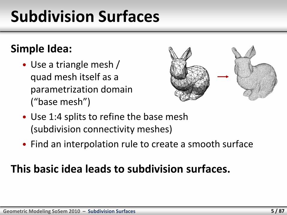
Simple Idea:
• Use a triangle mesh / quad mesh itself as a parametrization domain (“base mesh”)
• Use 1:4 splits to refine the base mesh (subdivision connectivity meshes)
• Find an interpolation rule to create a smooth surface
This basic idea leads to subdivision surfaces.

Geometric Modeling SoSem 2010 – Subdivision Surfaces 6 / 87
1.
Basic Scheme
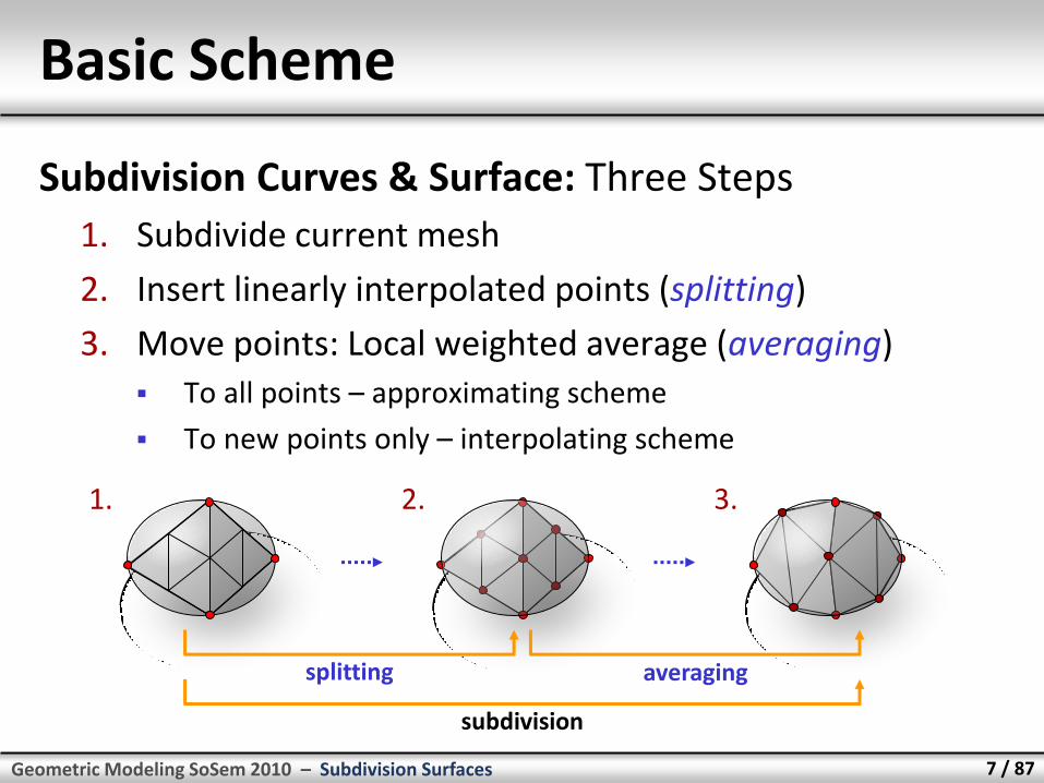
Subdivision Curves & Surface: Three Steps
1. Subdivide current mesh
2. Insert linearly interpolated points (splitting)
3. Move points: Local weighted average (averaging)
To all points – approximating scheme
To new points only – interpolating scheme
2. 3.
splitting averaging
subdivision
Geometric Modeling SoSem 2010 – Subdivision Surfaces 7 / 87
1.
Basic Scheme
Subdivision Curves & Surface: Three Steps
1. Subdivide current mesh
2. Insert linearly interpolated points (splitting)
3. Move points: Local weighted average (averaging)
To all points – approximating scheme
To new points only – interpolating scheme
2. 3.
splitting averaging
subdivision
Geometric Modeling SoSem 2010 – Subdivision Surfaces 8 / 87
Subdivision Surfaces
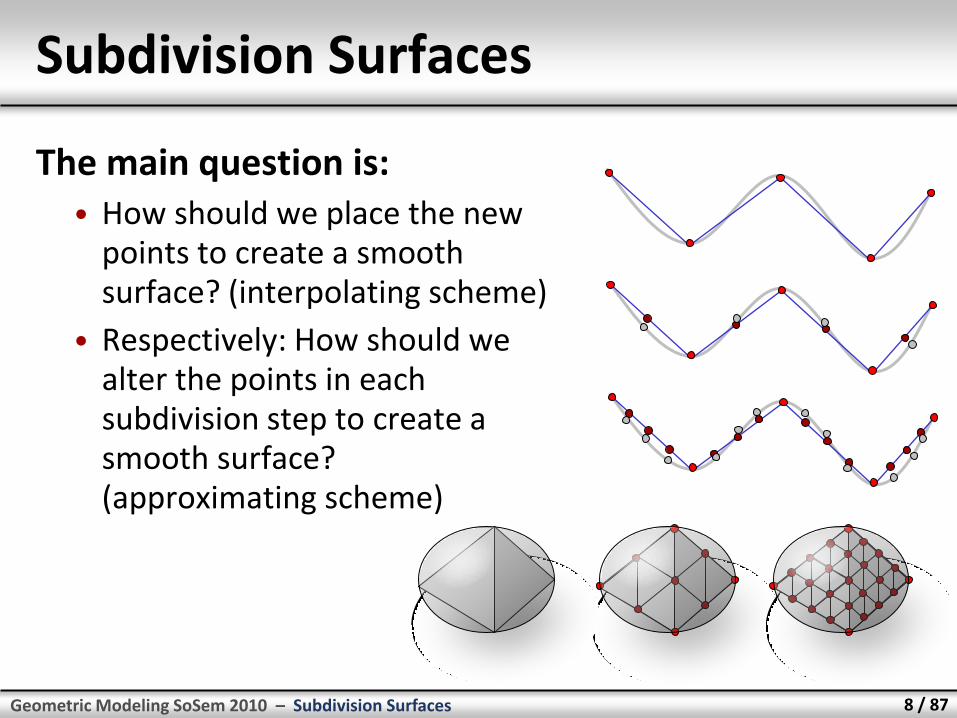
The main question is: • How should we place the new
points to create a smooth surface? (interpolating scheme)
• Respectively: How should we alter the points in each subdivision step to create a smooth surface? (approximating scheme)
Geometric Modeling SoSem 2010 – Subdivision Surfaces 9 / 87
Subdivision Schemes
More precisely:
• What are good averaging masks?
• The averaging mask determines the weights by which the new point positions are computed
Interesting observation:
• Most averaging schemes do not converge (in particular interpolating schemes – try this at home).
• We need to be very careful to design a good averaging mask.
• How can we guarantee C1, C2 surfaces?
Geometric Modeling SoSem 2010 – Subdivision Surfaces 10 / 87
Example: Corner Cutting
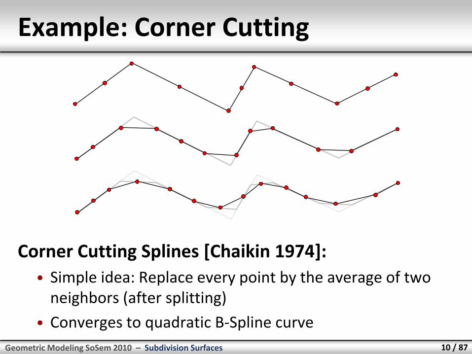
Corner Cutting Splines [Chaikin 1974]:
• Simple idea: Replace every point by the average of two neighbors (after splitting)
• Converges to quadratic B-Spline curve

Geometric Modeling SoSem 2010 – Subdivision Surfaces 11 / 87
p2i+1(l + 1) p2i-1
(l + 1)
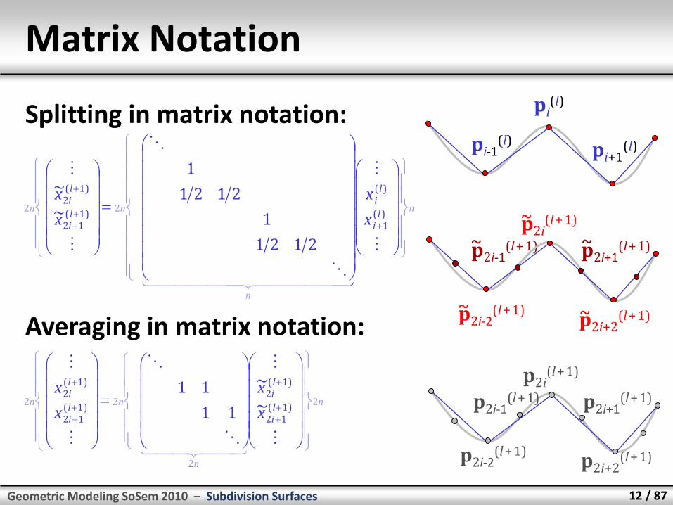
Matrix Notation
Curve subdivision in matrix notation:
• Control points
at level l: pi(l)
• “Splitted” points
at level l + 1: pi(l + 1)
• “Averaged” control points
at level l + 1: pi(l + 1)
~
p2i+1(l + 1)
pi(l)
pi-1(l)
pi+1(l)
p2i(l + 1)
p2i-2(l + 1)
p2i+2(l + 1)
~ ~ ~
~ ~
p2i(l + 1)
p2i-2(l + 1)
p2i+2(l + 1)
p2i-1(l + 1)
Geometric Modeling SoSem 2010 – Subdivision Surfaces 12 / 87
p2i+1(l + 1) p2i-1
(l + 1)
p2i+1(l + 1)
Matrix Notation
Splitting in matrix notation: pi(l)
pi-1(l)
pi+1(l)
p2i(l + 1)
p2i-2(l + 1)
p2i+2(l + 1)
~ ~ ~
~ ~
p2i(l + 1)
p2i-2(l + 1)
p2i+2(l + 1)
p2i-1(l + 1)
Averaging in matrix notation:
nl
i
li
n
nli
li
n
x
x
x
x
)(1
)(
2)1(
12
)1(2
2
2121
1
2121
1
~
~
nli
li
n
nli
li
n
x
x
x
x2
)1(12
)1(2
2
2)1(
12
)1(2
2 ~
~
11
11

B-Spline Subdivision Schemes (Regular Subdivision)

Geometric Modeling SoSem 2010 – Subdivision Surfaces 14 / 87
B-Spline Subdivision
1.0
0.8
0.6
0.4
0.2
0.0 1.0 2.0 3.0 4.0
uniform cubic B-spline basis function b(t)
gray: dilated functions b(2t + i)
1.0
0.8
0.6
0.4
0.2
0.0 1.0 2.0 3.0 4.0
expressed as sum of dilated functions b(t) = i ci b(2t + i)
Geometric Modeling SoSem 2010 – Subdivision Surfaces 15 / 87
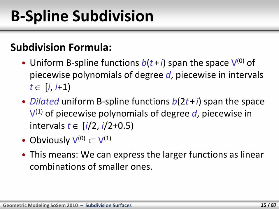
B-Spline Subdivision
Subdivision Formula:
• Uniform B-spline functions b(t + i) span the space V(0) of piecewise polynomials of degree d, piecewise in intervals t [i, i+1)
• Dilated uniform B-spline functions b(2t + i) span the space V(1) of piecewise polynomials of degree d, piecewise in intervals t [i/2, i/2+0.5)
• Obviously V(0) V(1)
• This means: We can express the larger functions as linear combinations of smaller ones.
Geometric Modeling SoSem 2010 – Subdivision Surfaces 16 / 87
Subdivision masks
Question: What are the coefficients for the linear combination?
Standard answer:
• Solve a linear system (underdetermined)
Direct derivation (arbitrary degree):
• We look at the definition of higher order basis functions by repeated convolution.
• By analyzing the effect of each further convolution, we get a subdivision formula by induction.

Geometric Modeling SoSem 2010 – Subdivision Surfaces 17 / 87
Repeated Convolution
Defining B-splines by repeated convolution (recap):
• We start with 0th degree basis functions
• Increase smoothness by convolution
Degree-zero B-spline:
General-degree B-spline:
otherwise ,0
)1...0[ if ,1)()0( t
tb
dxtxbxbtbtbtb iii )()()()()( )0()()0()()1(

Geometric Modeling SoSem 2010 – Subdivision Surfaces 18 / 87
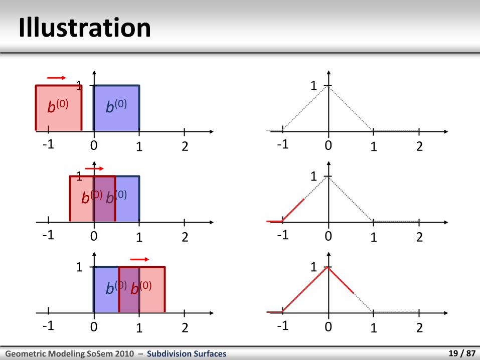
Repeated Convolution
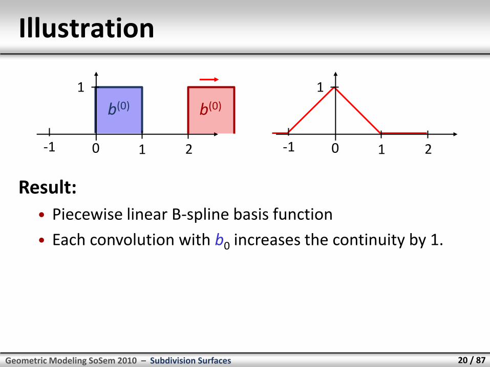
Convolution:
• Weighted average of functions
• Definition:
Example:
dxtxgxftgtf )()()()(
t
g f
Geometric Modeling SoSem 2010 – Subdivision Surfaces 19 / 87
Illustration
1
1 2 0 -1
b(0)
1
1 2 0 -1
b(0)
1
1 2 0 -1
b(0)
b(0)
1
1 2 0 -1
1
1 2 0 -1
1
1 2 0 -1
b(0)
b(0)
Geometric Modeling SoSem 2010 – Subdivision Surfaces 20 / 87
Illustration
1
1 2 0 -1
b(0)
1
1 2 0 -1
b(0)
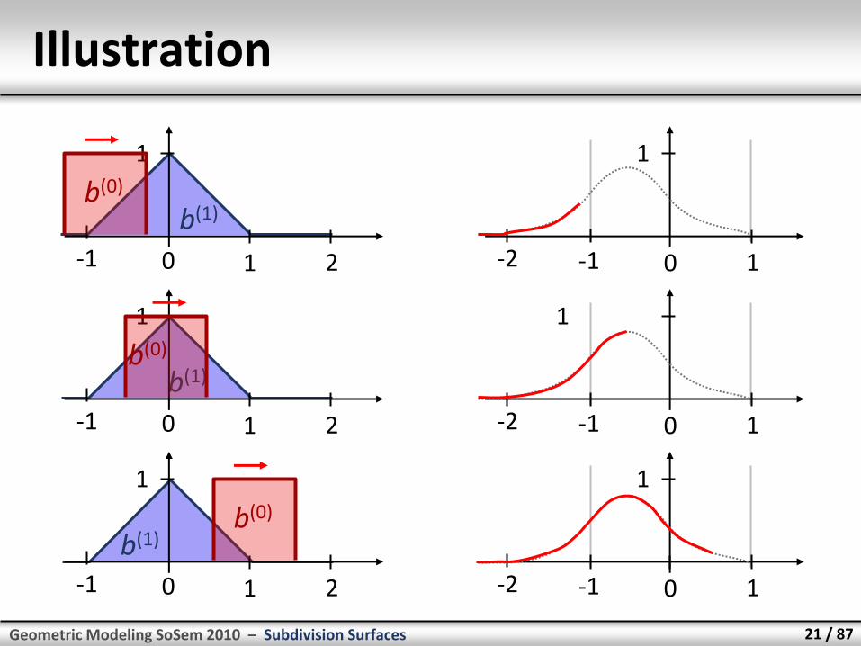
Result:
• Piecewise linear B-spline basis function
• Each convolution with b0 increases the continuity by 1.
Geometric Modeling SoSem 2010 – Subdivision Surfaces 21 / 87
b(1)
b(1)
Illustration
1
1 2 0 -1
b(1)
1
1 2 0 -1
1
1 2 0 -1
b(0)
1
0 1 -1 -2
1
0 1 -1 -2
1
0 1 -1 -2
b(0)
b(0)
Geometric Modeling SoSem 2010 – Subdivision Surfaces 22 / 87
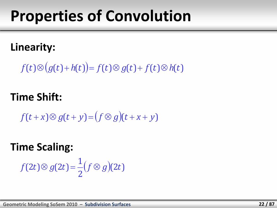
Properties of Convolution
Linearity:
Time Shift:
Time Scaling:
)()()()()()()( thtftgtfthtgtf
)()()( yxtgfytgxtf
)2(2
1)2()2( tgftgtf
Geometric Modeling SoSem 2010 – Subdivision Surfaces 23 / 87
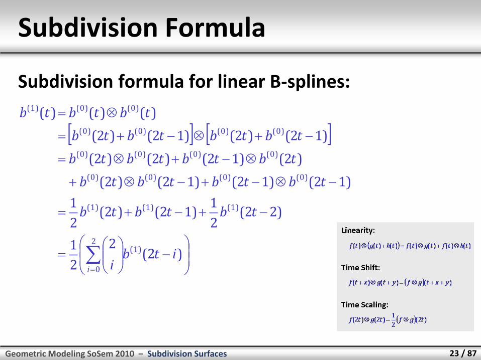
Subdivision Formula
Subdivision formula for linear B-splines:
2
0
)1(
)1()1()1(
)0()0()0()0(
)0()0()0()0(
)0()0()0()0(
)0()0()1(
)2(2
2
1
)22(2
1)12()2(
2
1
)12()12()12()2(
)2()12()2()2(
)12()2()12()2(
)()()(
i
itbi
tbtbtb
tbtbtbtb
tbtbtbtb
tbtbtbtb
tbtbtb
Geometric Modeling SoSem 2010 – Subdivision Surfaces 24 / 87
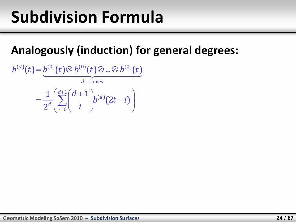
Subdivision Formula
Analogously (induction) for general degrees:
1
0
)(
times 1
)0()0()0()(
)2(1
2
1
)(...)()()(
d
i
d
d
d
d
itbi
d
tbtbtbtb
Geometric Modeling SoSem 2010 – Subdivision Surfaces 25 / 87
1
0
)()( )(21
2
1)(
d
i
d
d
d ijtbi
djtb
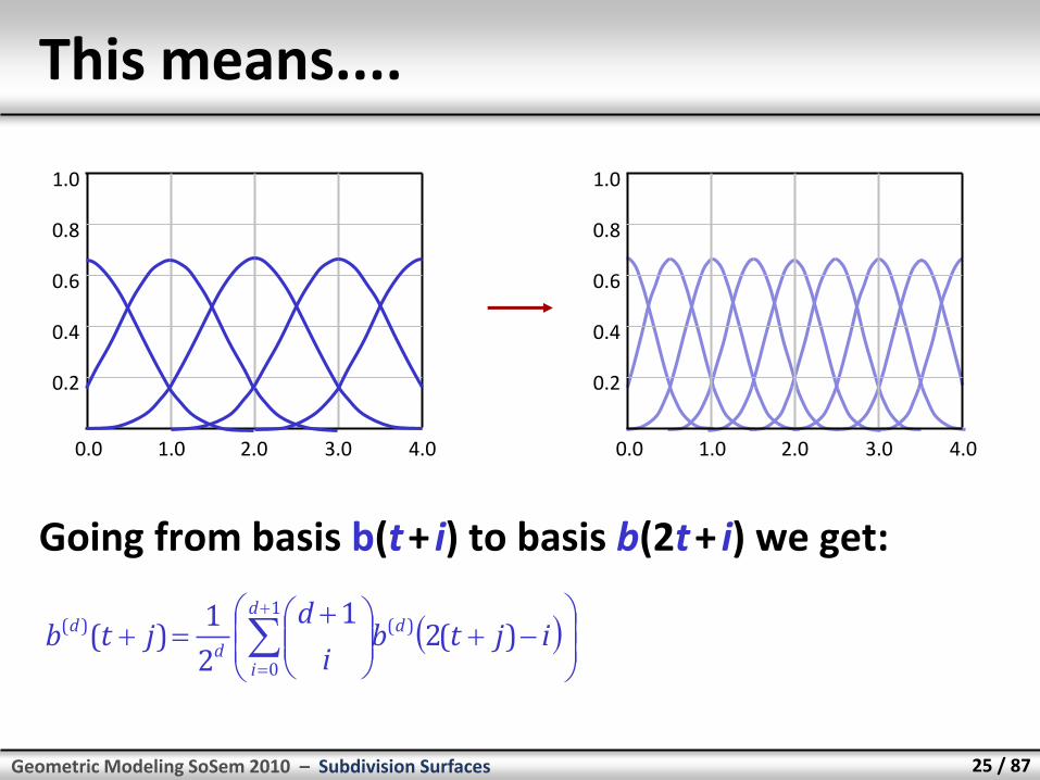
This means....
Going from basis b(t + i) to basis b(2t + i) we get:
1.0
0.8
0.6
0.4
0.2
0.0 1.0 2.0 3.0 4.0
1.0
0.8
0.6
0.4
0.2
0.0 1.0 2.0 3.0 4.0

Geometric Modeling SoSem 2010 – Subdivision Surfaces 26 / 87
428
1
328
4
228
6
128
4
28
1)(
)3(
)3(
)3(
)3(
)3()3(
tb
tb
tb
tb
tbtb
Example
1.0
0.8
0.6
0.4
0.2
0.0 1.0 2.0 3.0 4.0
1.0
0.8
0.6
0.4
0.2
0.0 1.0 2.0 3.0 4.0
Cubic case:
8
1
8
4
8
6
8
1
8
4
Geometric Modeling SoSem 2010 – Subdivision Surfaces 27 / 87
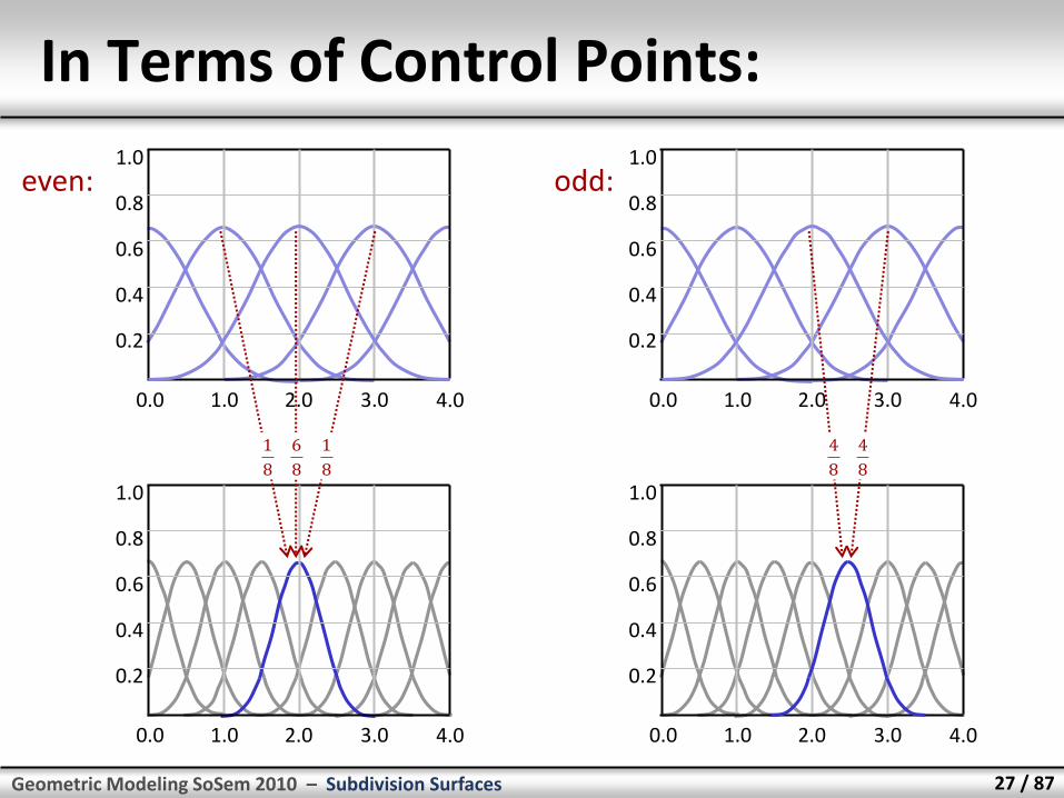
In Terms of Control Points:
1.0
0.8
0.6
0.4
0.2
0.0 1.0 2.0 3.0 4.0
1.0
0.8
0.6
0.4
0.2
0.0 1.0 2.0 3.0 4.0
8
4
1.0
0.8
0.6
0.4
0.2
0.0 1.0 2.0 3.0 4.0
1.0
0.8
0.6
0.4
0.2
0.0 1.0 2.0 3.0 4.0
8
1
8
6
8
1
8
4
even: odd:

Geometric Modeling SoSem 2010 – Subdivision Surfaces 28 / 87
In Terms of Control Points:
1.0
0.8
0.6
0.4
0.2
0.0 1.0 2.0 3.0 4.0
1.0
0.8
0.6
0.4
0.2
0.0 1.0 2.0 3.0 4.0
2
1
1.0
0.8
0.6
0.4
0.2
0.0 1.0 2.0 3.0 4.0
1.0
0.8
0.6
0.4
0.2
0.0 1.0 2.0 3.0 4.0
8
1
4
3
8
1
even: odd:
2
1
Geometric Modeling SoSem 2010 – Subdivision Surfaces 29 / 87
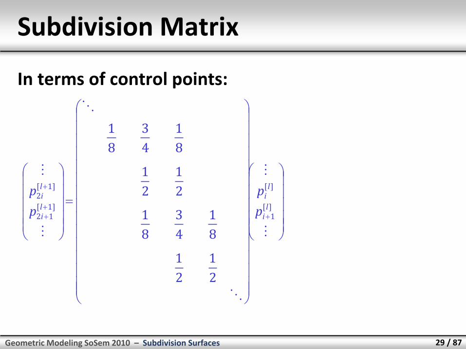
Subdivision Matrix
In terms of control points:
][1
][
]1[12
]1[2
2
1
2
1
8
1
4
3
8
1
2
1
2
1
8
1
4
3
8
1
li
li
li
li
p
p
p
p

Geometric Modeling SoSem 2010 – Subdivision Surfaces 30 / 87
Splitting and Averaging
So far:
• Splitting & averaging in one step
p2i+1(l + 1) p2i-1
(l + 1)
p2i+1(l + 1)
pi(l)
pi-1(l)
pi+1(l)
p2i(l + 1)
p2i-2(l + 1)
p2i+2(l + 1)
~ ~ ~
~ ~
p2i(l + 1)
p2i-2(l + 1)
p2i+2(l + 1)
p2i-1(l + 1)
][1
][
]1[12
]1[2
2
1
2
1
8
1
4
3
8
1
2
1
2
1
8
1
4
3
8
1
li
li
li
li
p
p
p
p
Geometric Modeling SoSem 2010 – Subdivision Surfaces 31 / 87
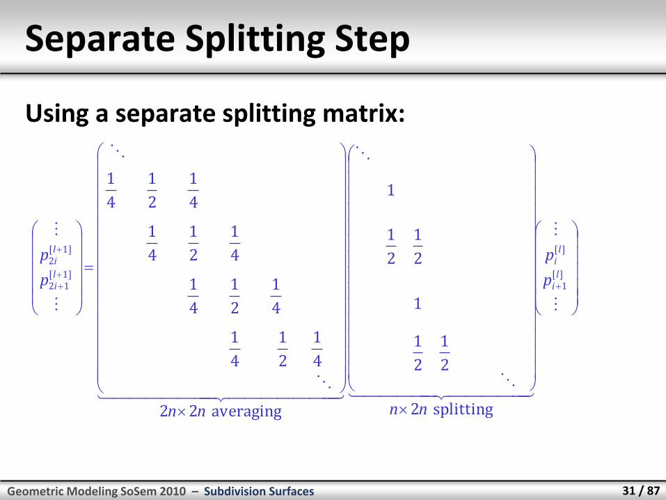
Separate Splitting Step
Using a separate splitting matrix:
][1
][
]1[12
]1[2
splitting 2
2
1
2
1
1
2
1
2
1
1
averaging 22
4
1
2
1
4
1
4
1
2
1
4
1
4
1
2
1
4
1
4
1
2
1
4
1
li
li
li
li
p
p
nnnn
p
p
Geometric Modeling SoSem 2010 – Subdivision Surfaces 32 / 87
][1
][
]1[12
]1[2
splitting 2
2
1
2
1
1
2
1
2
1
1
averaging 22
4
1
2
1
4
1
4
1
2
1
4
1
4
1
2
1
4
1
4
1
2
1
4
1
li
li
li
li
p
p
nnnn
p
p
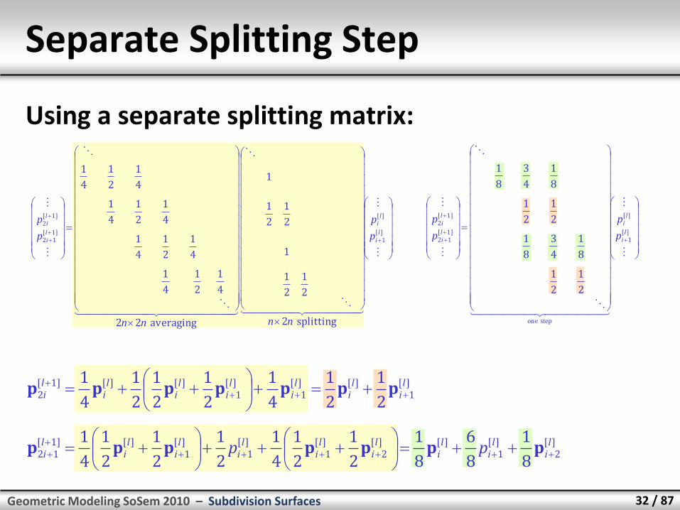
Separate Splitting Step
Using a separate splitting matrix:
][1
][][1
][1
][][]1[2
2
1
2
1
4
1
2
1
2
1
2
1
4
1 li
li
li
li
li
li
li
ppppppp
][2
][1
][][2
][1
][1
][1
][]1[12
8
1
8
6
8
1
2
1
2
1
4
1
2
1
2
1
2
1
4
1 li
li
li
li
li
li
li
li
li pp
ppppppp
][1
][
step one
]1[12
]1[2
2
1
2
1
8
1
4
3
8
1
2
1
2
1
8
1
4
3
8
1
li
li
li
li
p
p
p
p
Geometric Modeling SoSem 2010 – Subdivision Surfaces 33 / 87
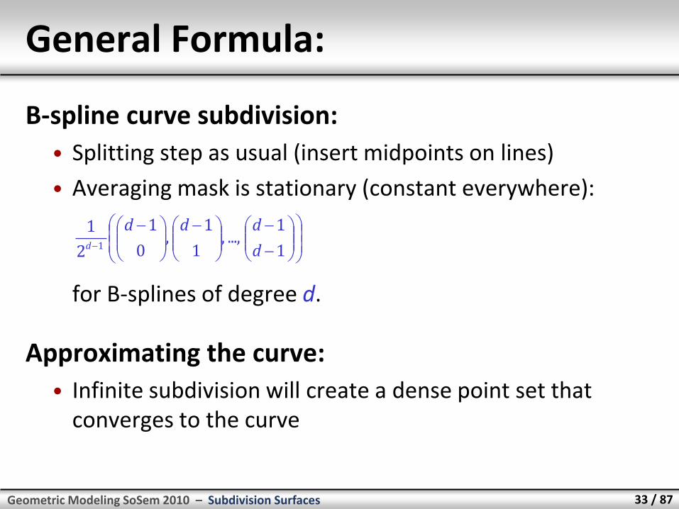
General Formula:
B-spline curve subdivision:
• Splitting step as usual (insert midpoints on lines)
• Averaging mask is stationary (constant everywhere):
for B-splines of degree d.
Approximating the curve:
• Infinite subdivision will create a dense point set that converges to the curve
1
1...,,
1
1,
0
1
2
11 d
dddd

Spectral Convergence Analysis
Geometric Modeling SoSem 2010 – Subdivision Surfaces 35 / 87
The Spectral Limit Trick
Problem:
• We need to subdivide several times to obtain a good approximation
• This might yield more control points that necessary (think of adaptive rendering with low level of detail)
• Can we directly compute the limit position for a control point?
Geometric Modeling SoSem 2010 – Subdivision Surfaces 36 / 87
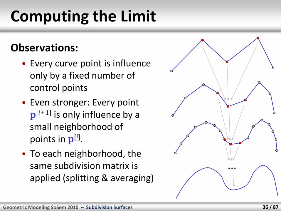
Computing the Limit
Observations:
• Every curve point is influence only by a fixed number of control points
• Even stronger: Every point p[l + 1] is only influence by a small neighborhood of points in p[l].
• To each neighborhood, the same subdivision matrix is applied (splitting & averaging)
...
Geometric Modeling SoSem 2010 – Subdivision Surfaces 37 / 87
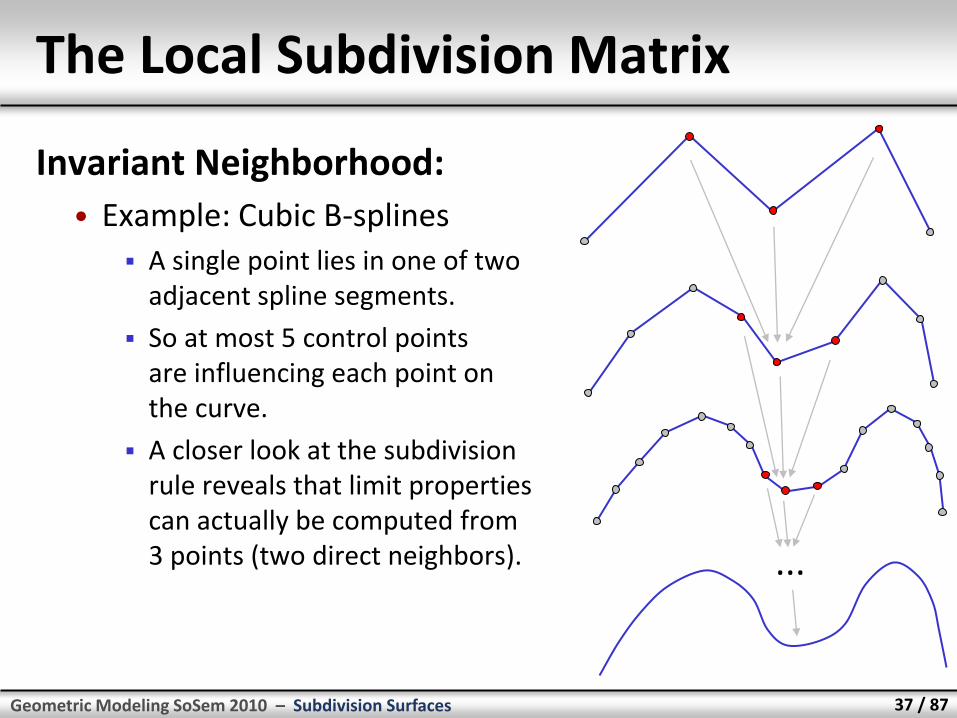
The Local Subdivision Matrix
Invariant Neighborhood:
• Example: Cubic B-splines
A single point lies in one of two adjacent spline segments.
So at most 5 control points are influencing each point on the curve.
A closer look at the subdivision rule reveals that limit properties can actually be computed from 3 points (two direct neighbors). ...

Geometric Modeling SoSem 2010 – Subdivision Surfaces 38 / 87
Local Subdivision Matrix
Local subdivision matrix:
• Transforms a neighborhood of points
Example: Cubic B-Spline
• Only the two direct neighbors influence the point in the next level
• The local subdivision matrix is: x- = left neighbor x = point (x/y/z-coordinate) x+ = right neighbor
][
][
][
:
]1[
]1[
]1[
2
1
2
10
8
1
4
3
8
1
02
1
2
1
l
l
l
l
l
l
x
x
x
x
x
x
subdiv
M
Geometric Modeling SoSem 2010 – Subdivision Surfaces 39 / 87
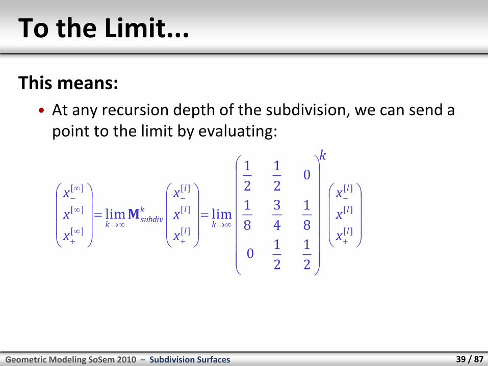
To the Limit...
This means:
• At any recursion depth of the subdivision, we can send a point to the limit by evaluating:
][
][
][
][
][
][
][
][
][
2
1
2
10
8
1
4
3
8
1
02
1
2
1
limliml
l
l
kl
l
l
ksubdiv
k
x
x
x
k
x
x
x
x
x
x
M
Geometric Modeling SoSem 2010 – Subdivision Surfaces 40 / 87
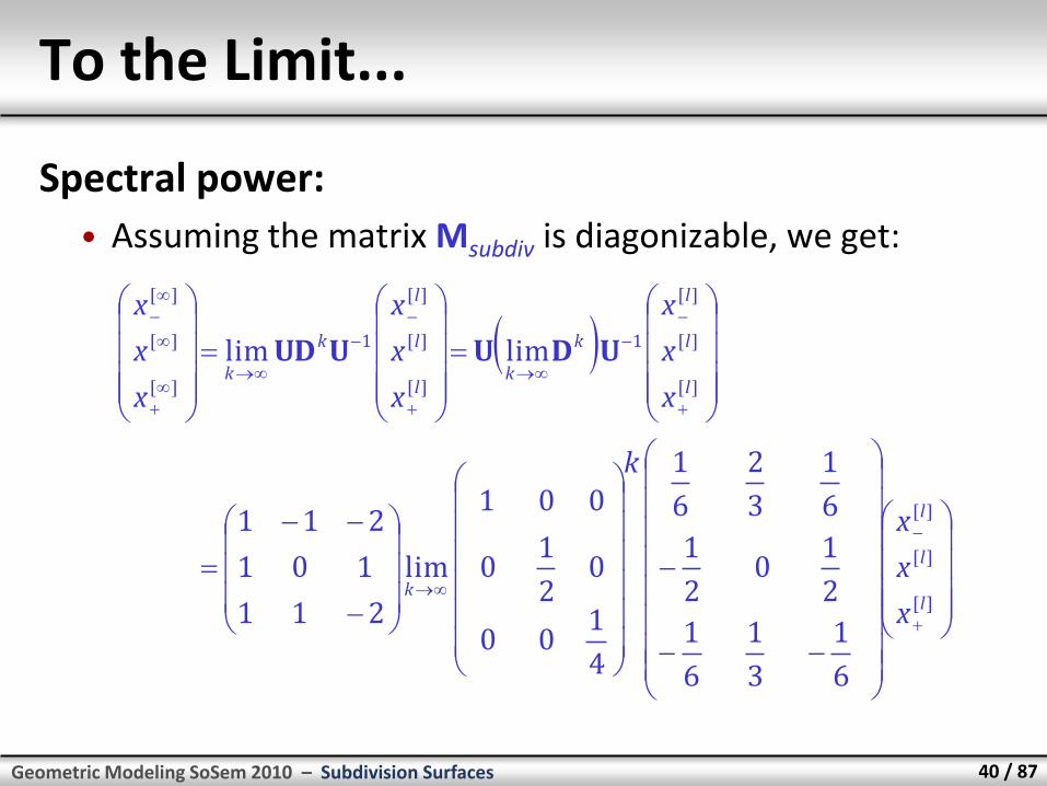
To the Limit...
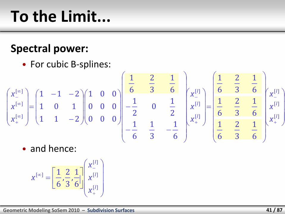
Spectral power:
• Assuming the matrix Msubdiv is diagonizable, we get:
][
][
][
][
][
][
1
][
][
][
1
][
][
][
6
1
3
1
6
1
2
10
2
1
6
1
3
2
6
1
4
100
02
10
001
lim
211
101
211
limlim
l
l
l
k
l
l
l
k
kl
l
l
k
k
x
x
x
k
x
x
x
x
x
x
x
x
x
UDUUUD
Geometric Modeling SoSem 2010 – Subdivision Surfaces 41 / 87
To the Limit...
Spectral power:
• For cubic B-splines:
][
][
][
][
][
][
][
][
][
6
1
3
2
6
1
6
1
3
2
6
1
6
1
3
2
6
1
6
1
3
1
6
1
2
10
2
1
6
1
3
2
6
1
000
000
001
211
101
211
l
l
l
l
l
l
x
x
x
x
x
x
x
x
x
][
][
][
][
6
1,
3
2,
6
1
l
l
l
x
x
x
x
• and hence:
Geometric Modeling SoSem 2010 – Subdivision Surfaces 42 / 87
To the Limit, in General
In general:
• The dominant eigenvalue / eigenvector of the subdivision scheme determines the limit mask
Geometric Modeling SoSem 2010 – Subdivision Surfaces 43 / 87
Necessary Condition
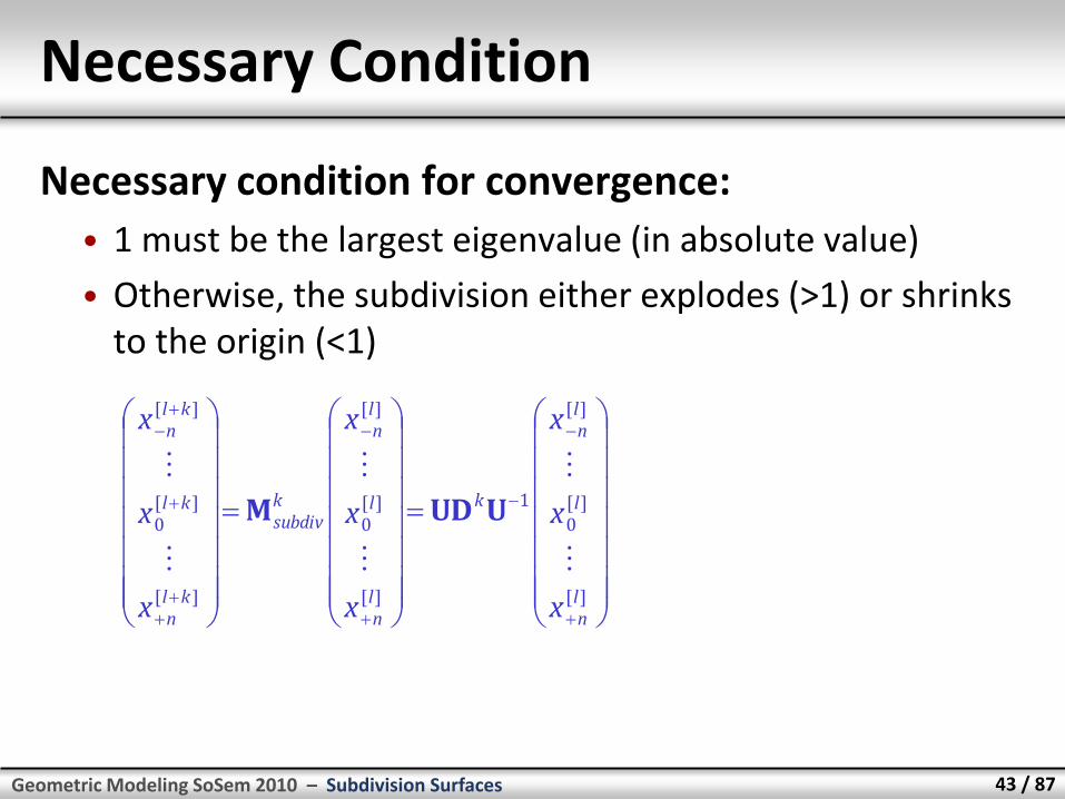
Necessary condition for convergence:
• 1 must be the largest eigenvalue (in absolute value)
• Otherwise, the subdivision either explodes (>1) or shrinks to the origin (<1)
][
][0
][
1
][
][0
][
][
][0
][
ln
l
ln
k
ln
l
ln
ksubdiv
kln
kl
kln
x
x
x
x
x
x
x
x
x
UUDM
Geometric Modeling SoSem 2010 – Subdivision Surfaces 44 / 87
2
1
2
10
8
1
8
6
8
1
02
1
2
1
Affine Invariance
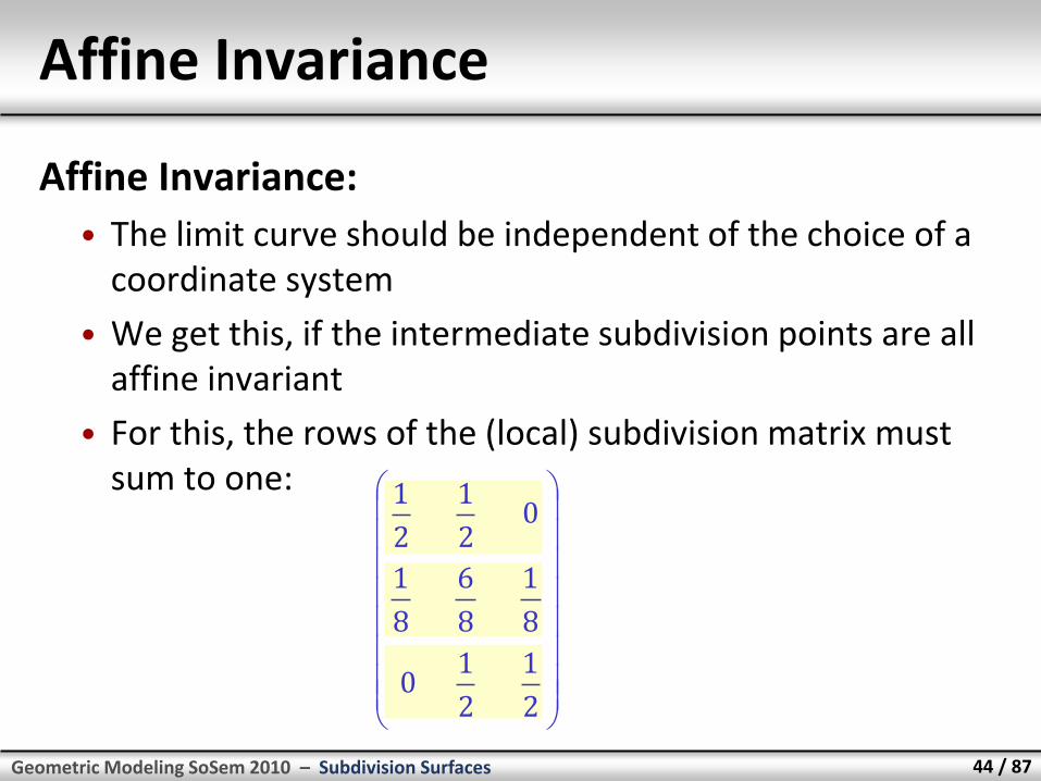
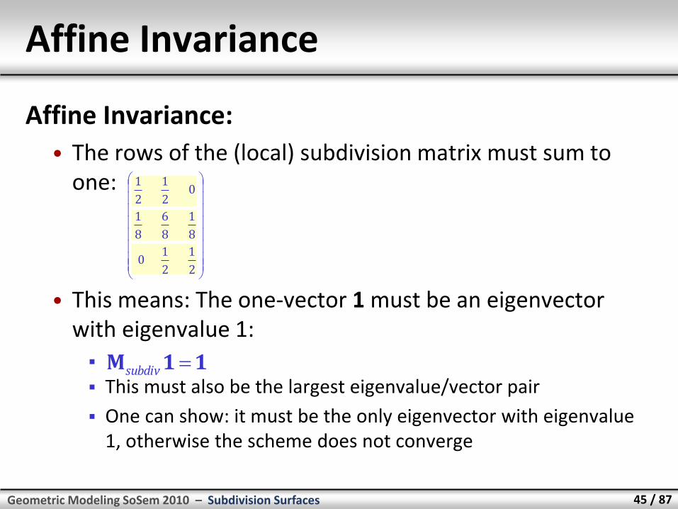
Affine Invariance:
• The limit curve should be independent of the choice of a coordinate system
• We get this, if the intermediate subdivision points are all affine invariant
• For this, the rows of the (local) subdivision matrix must sum to one:
Geometric Modeling SoSem 2010 – Subdivision Surfaces 45 / 87
2
1
2
10
8
1
8
6
8
1
02
1
2
1
Affine Invariance
Affine Invariance:
• The rows of the (local) subdivision matrix must sum to one:
• This means: The one-vector 1 must be an eigenvector with eigenvalue 1:
This must also be the largest eigenvalue/vector pair
One can show: it must be the only eigenvector with eigenvalue 1, otherwise the scheme does not converge
11M subdiv

Geometric Modeling SoSem 2010 – Subdivision Surfaces 46 / 87
Derivatives
One can show:
• The tangent vectors are related to the second largest eigenvalue
• Intuition:
Difference to neighboring points is zero for first eigenvalue/eigenvector in the limit
Second largest shrinks faster, spreads the tangent direction
• For a C1 continuous curve, the second largest eigenvalue must be unique (only one eigenvector). This is a necessary condition.
Geometric Modeling SoSem 2010 – Subdivision Surfaces 47 / 87
Summary
For a reasonable subdivision scheme, we need at least:
• 1 must be a eigenvector with eigenvalue 1.
• This must be the largest eigenvalue.
• The second eigenvalue should be smaller than 1.
• All other eigenvalues should be smaller than the second one.
(This is assuming a diagonizable subdivision matrix.)
More details: Zorin, Schröder – Subdivision for Modeling and Animation, Siggraph 2000 course, available online (use Google).
B-Spline Subdivision Surfaces
Geometric Modeling SoSem 2010 – Subdivision Surfaces 49 / 87
B-Spline Subdivision Surfaces
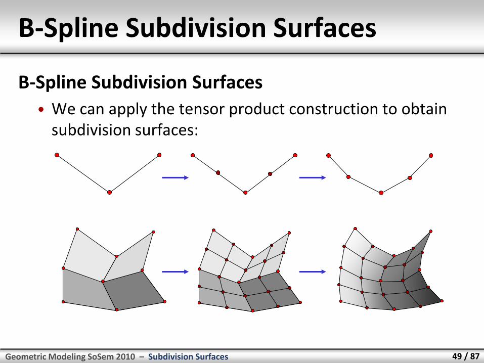
B-Spline Subdivision Surfaces
• We can apply the tensor product construction to obtain subdivision surfaces:
Geometric Modeling SoSem 2010 – Subdivision Surfaces 50 / 87
B-Spline Subdivision Surfaces
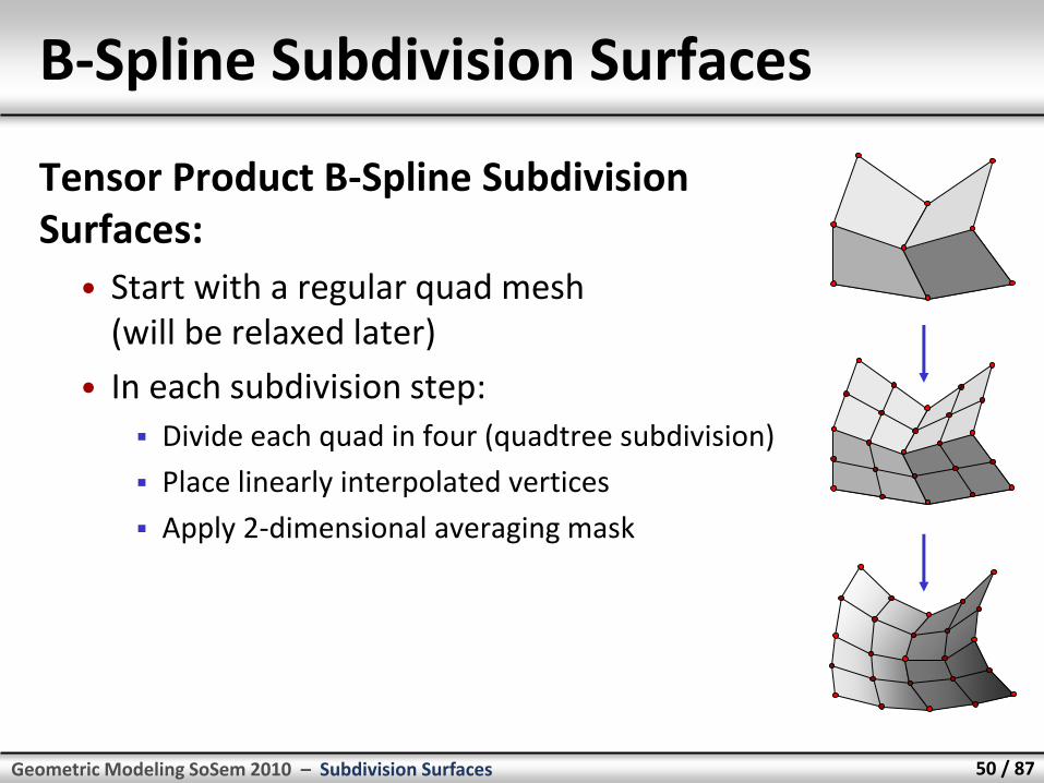
Tensor Product B-Spline Subdivision Surfaces:
• Start with a regular quad mesh (will be relaxed later)
• In each subdivision step:
Divide each quad in four (quadtree subdivision)
Place linearly interpolated vertices
Apply 2-dimensional averaging mask

Geometric Modeling SoSem 2010 – Subdivision Surfaces 51 / 87
32
3
16
1
16
1
16
1
Subdivision and Averaging Masks
What is the subdivision mask?
• Can be derived from tensor product construction:
face midpoint (odd/odd)
4
1
4
1
4
1
4
1
edge midpoint (even/odd)
16
1
8
3
original vertex (even/even)
8
3
64
1
32
3
64
1
64
1
64
1
32
3
32
3
16
9
2
1,
2
1
2
12
1
8
1,
4
3,
8
1
2
12
1
8
1,
4
3,
8
1
8
1
4
3
8
1
Geometric Modeling SoSem 2010 – Subdivision Surfaces 52 / 87
8
1
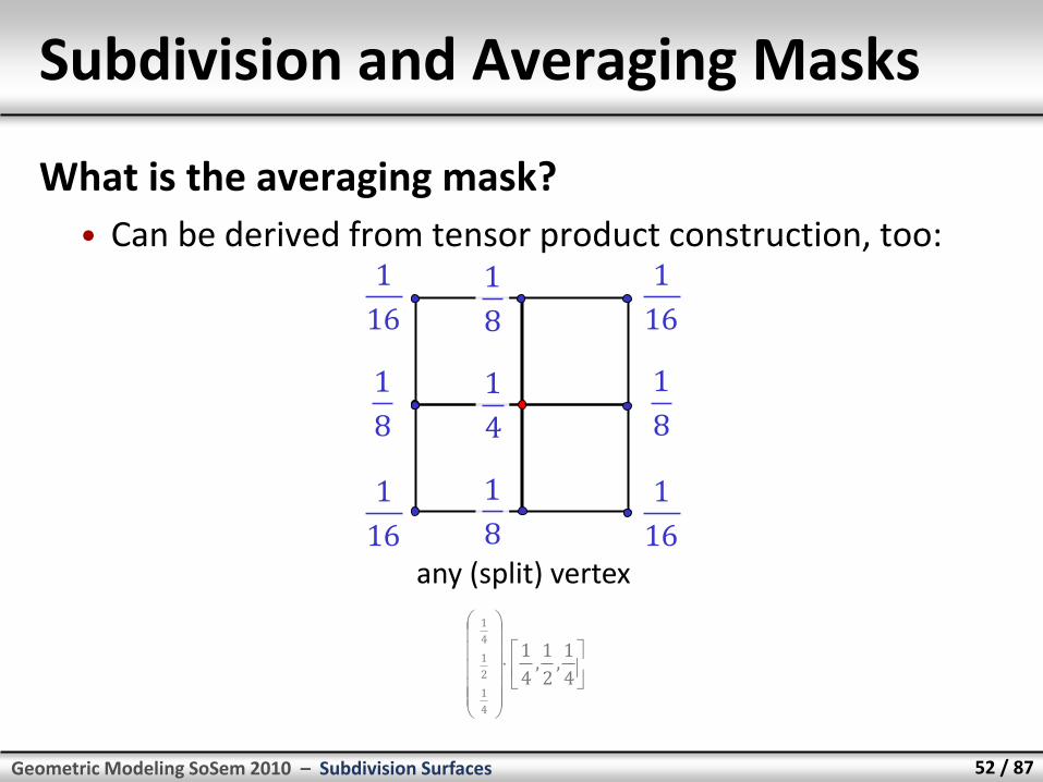
Subdivision and Averaging Masks
What is the averaging mask?
• Can be derived from tensor product construction, too:
any (split) vertex
16
1
8
1
16
1
16
1
16
1
8
1
8
1
4
1
4
1,
2
1,
4
1
4
1
2
1
4
1

Geometric Modeling SoSem 2010 – Subdivision Surfaces 53 / 87
Generalizations
Generalizations:
• General degree B-spline tensor product surface subdivision rules can be derived in the same way
• Just use the 1-dimensional subdivision / averaging masks and form a tensor product mask
• Guaranteed to converge to a Cd-1-smooth surface
• Ok, but something is missing...
Geometric Modeling SoSem 2010 – Subdivision Surfaces 54 / 87
Remaining Problems
Remaining Problems:
• The derived rules work only in the interior or a regular quad mesh
• We did not really gain any flexibility over the standard B-spline construction
• We still need to figure out, how to...:
...handle quad meshes of arbitrary topology.
...handle boundary regions.
– Placing boundaries in the interior of objects will allow us to model sharp C0 creases
– So we also have some continuity control (despite the uniform B-Spline scheme)
Geometric Modeling SoSem 2010 – Subdivision Surfaces 55 / 87
Here is the answer...
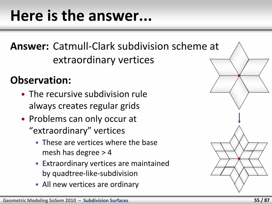
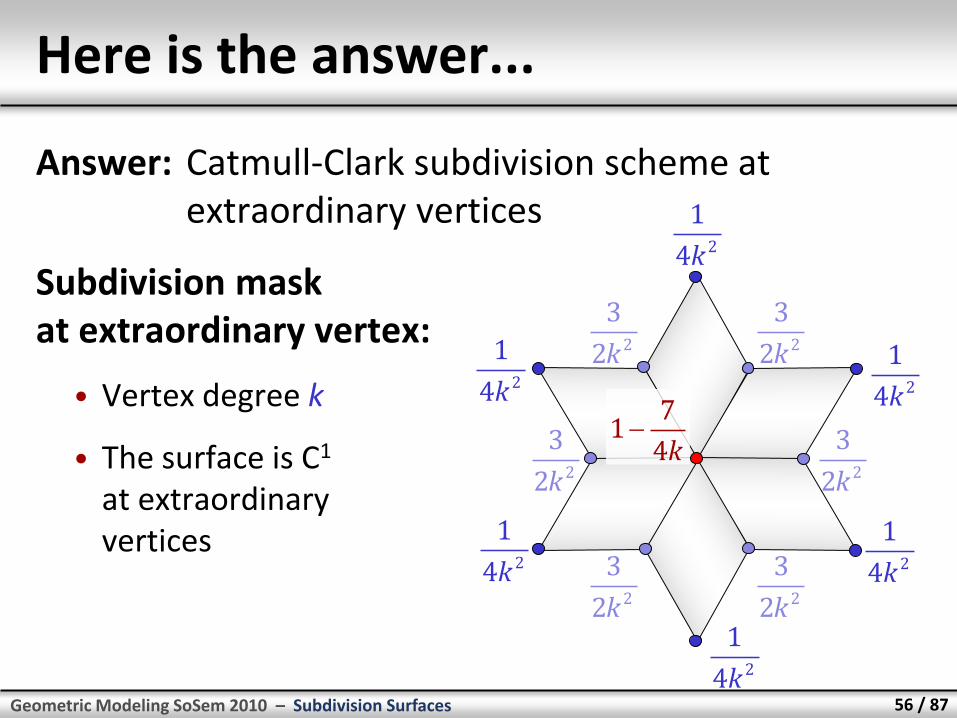
Answer: Catmull-Clark subdivision scheme at extraordinary vertices
Observation: • The recursive subdivision rule
always creates regular grids
• Problems can only occur at “extraordinary” vertices
These are vertices where the base mesh has degree > 4
Extraordinary vertices are maintained by quadtree-like-subdivision
All new vertices are ordinary
Geometric Modeling SoSem 2010 – Subdivision Surfaces 56 / 87
Here is the answer...
Answer: Catmull-Clark subdivision scheme at extraordinary vertices
Subdivision mask at extraordinary vertex:
• Vertex degree k
• The surface is C1 at extraordinary vertices
24
1
k
22
3
k
24
1
k
24
1
k 24
1
k
24
1
k
24
1
k
22
3
k
22
3
k22
3
k
22
3
k 22
3
k
k4
71
Geometric Modeling SoSem 2010 – Subdivision Surfaces 57 / 87
Here is the answer...
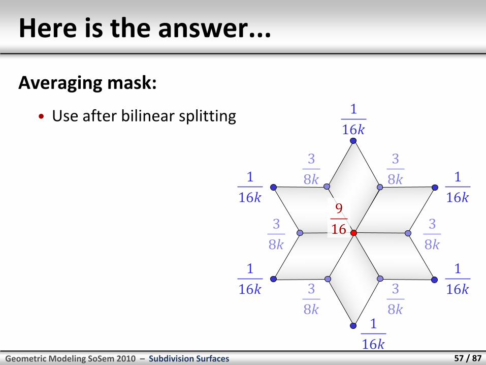
Averaging mask:
• Use after bilinear splitting
k8
3
k16
1
16
9k16
1
k16
1
k16
1
k16
1
k16
1
k8
3
k8
3
k8
3
k8
3
k8
3
Geometric Modeling SoSem 2010 – Subdivision Surfaces 58 / 87
Boundary Rules
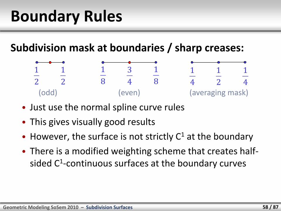
Subdivision mask at boundaries / sharp creases:
• Just use the normal spline curve rules
• This gives visually good results
• However, the surface is not strictly C1 at the boundary
• There is a modified weighting scheme that creates half-sided C1-continuous surfaces at the boundary curves
2
1
2
1
8
1
4
3
8
1
(odd) (even) 4
1
2
1
4
1
(averaging mask)

Other Subdivision Schemes Loop, Butterfly, ...
Geometric Modeling SoSem 2010 – Subdivision Surfaces 60 / 87
Subdivision Zoo
A large number of subdivision schemes exists. The most popular are:
• Catmull-Clark subdivsion (quad-mesh, approximating, C2 surfaces, C1 at extraordinary vertices)
• Loop subdivsion (triangular, approximating, C2 surfaces, C1 at extraordinary vertices)
• Butterfly subdivsion (triangular, interpolation, C1 surfaces, C1 at extraordinary vertices)
Examples of other schemes:
• 3 – subdivision (level of detail increases more slowly)
• Circular subdivision (used e.g. for surfaces of revolution)
Geometric Modeling SoSem 2010 – Subdivision Surfaces 61 / 87
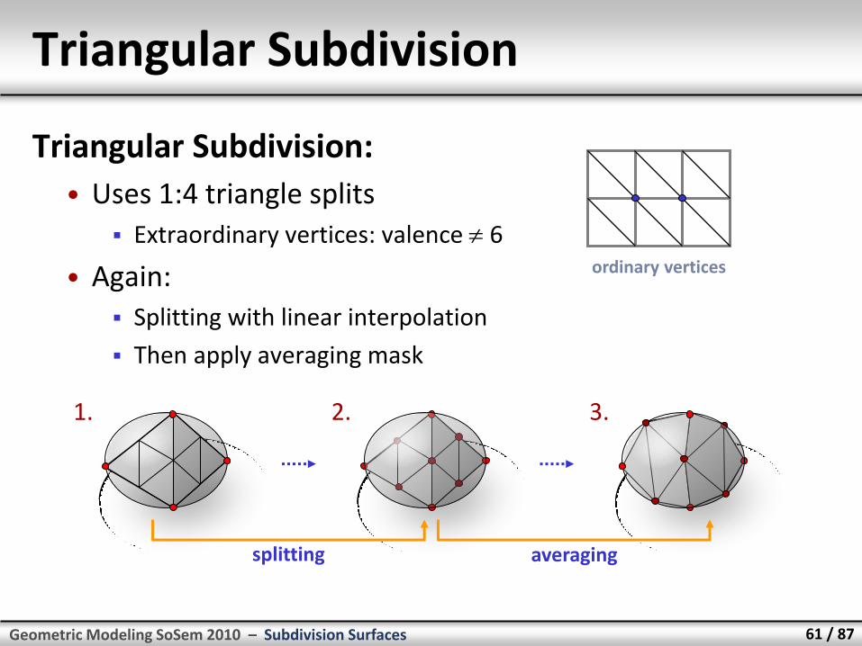
Triangular Subdivision
Triangular Subdivision:
• Uses 1:4 triangle splits
Extraordinary vertices: valence 6
• Again:
Splitting with linear interpolation
Then apply averaging mask
1. 2. 3.
splitting averaging
ordinary vertices
Geometric Modeling SoSem 2010 – Subdivision Surfaces 62 / 87
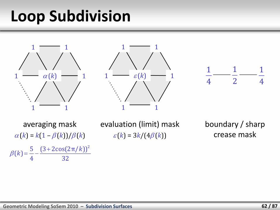
Loop Subdivision
(k)
1
1
1
1
1 1 (k)
1
1
1
1
1 1
averaging mask
(k) = k(1 – (k))/ (k)
32
))π/2cos(23(
4
5)(
2kk
evaluation (limit) mask
(k) = 3k/(4 (k))
4
1
2
1
4
1
boundary / sharp crease mask

Geometric Modeling SoSem 2010 – Subdivision Surfaces 63 / 87
Loop Subdivision
0
tangent mask 1
2
4
1
5
6 3
2
4
1
5
6 3
tangent mask 2
0
2
4
1
5
6 3
1
3
k
4
5 2
i = cos(2i/k)
Geometric Modeling SoSem 2010 – Subdivision Surfaces 64 / 87
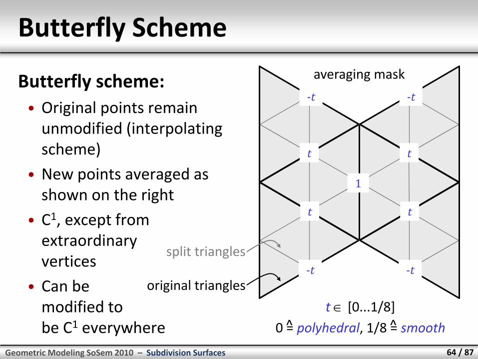
Butterfly Scheme
Butterfly scheme:
• Original points remain unmodified (interpolating scheme)
• New points averaged as shown on the right
• C1, except from extraordinary vertices
• Can be modified to be C1 everywhere
t
t
-t
-t
t
t
-t
-t
1
t [0...1/8]
0 = polyhedral, 1/8 = smooth ^ ^
original triangles
split triangles
averaging mask
Connection to Wavelet Nested Function Spaces and Wavelet Bases
Geometric Modeling SoSem 2010 – Subdivision Surfaces 66 / 87
Wavelets
Wavelets:
• Wavelet bases are an interesting tool that is very useful in computer graphics (and many other fields)
• Main idea:
Define a basis for a function space
Separate large scale from fine scale information
“Level-of-detail” basis
This allows for compression, scale-dependent processing and often leads to numerical more efficient and stable algorithms (e.g. wavelet preconditioning)
Geometric Modeling SoSem 2010 – Subdivision Surfaces 67 / 87
Nested Function Space
Starting Point:
• We consider a set of nested function spaces: V0 V1 ... Vi ...
• This means: with increasing index, a larger number of functions can be represented.
• We can find a basis Bi for Vi and Bi+1 for Vi+1 such that Bi Bi+1.
Geometric Modeling SoSem 2010 – Subdivision Surfaces 68 / 87
Special Spaces
We consider a special case:
• The basis functions in Bi are dilates of one and the same “mother” basis function (t):
ij = (2jt – i)
Bj = {ij}i
• The ij(t) are called scaling functions.
• With increaing j, the scaling functions should provide a more detailed representation of the same function.
• In order to achieve this, we need an additional property...
Geometric Modeling SoSem 2010 – Subdivision Surfaces 69 / 87
Subdivision Property
Nested Spaces:
• We want to have span(Bj) span(Bj+1).
• For this, we need to be able to reproduce the ij by linear
combinations of functions ij+1.
• This is the same condition we need for our geometric subdivision schemes.
• This means: Each subdivision scheme creates a corresponding nested scaling space (and vice versa).
Geometric Modeling SoSem 2010 – Subdivision Surfaces 70 / 87
Wavelet Bases
What we get so far:
• The span of the set B0 B1 ... Bn can describe functions at various level of detail.
• Problem:
This is not a basis. The set is still redundant.
The finest resolution set would be sufficient.
• Solution:
Remove redundant functions
Store only differences
Geometric Modeling SoSem 2010 – Subdivision Surfaces 71 / 87
Wavelet Bases
Constructing a wavelet basis:
• Start with V0 = span(B0). Add all {i0}i to the wavelet basis.
• Then add wavelet basis functions {i1}i that form a basis
of V1 \ V0 to this set.
• Continue with the next level of wavelets {i1}i that form a
basis of V2 \ V1.
• And so on.
Same structure:
• We again want a dilation property: ij = (2jt – i)
• (t) is called the “mother wavelet”
Geometric Modeling SoSem 2010 – Subdivision Surfaces 72 / 87
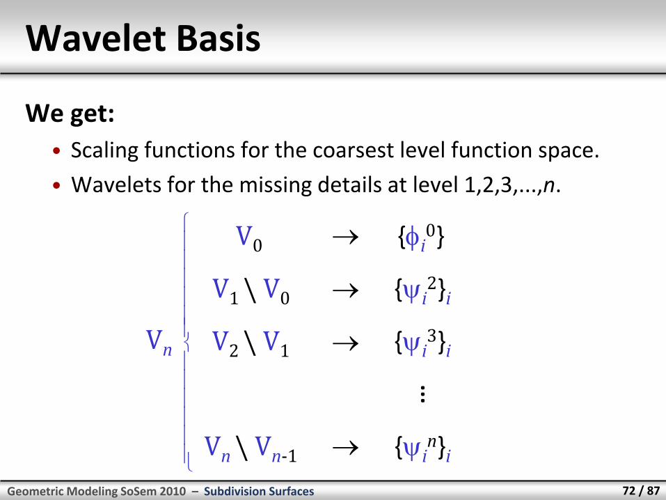
Wavelet Basis
{i0}
{i2}i
{i3}i
{in}i
... V0
V1 \ V0
V2 \ V1
Vn \ Vn-1
Vn
We get:
• Scaling functions for the coarsest level function space.
• Wavelets for the missing details at level 1,2,3,...,n.
Geometric Modeling SoSem 2010 – Subdivision Surfaces 73 / 87
Wavelet Basis Construction
How to choose the wavelet basis?
• Assume we are given the scaling functions.
• We (usually) still have a lot of freedom for choosing the wavelet basis.
• Desirable properties:
Small support (efficiency)
Orthogonality (good for compression)
Symmetry (useful for signal processing)
High order of smoothness (depends on scaling function)
• Not all can be obtained at the same time
• Various compromises have been proposed in literature
Geometric Modeling SoSem 2010 – Subdivision Surfaces 74 / 87
Example: Haar basis
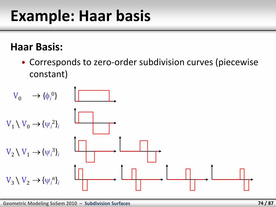
Haar Basis:
• Corresponds to zero-order subdivision curves (piecewise constant)
{i0} V0
{i2}i V1 \ V0
{in}i V3 \ V2
{i3}i V2 \ V1
Geometric Modeling SoSem 2010 – Subdivision Surfaces 75 / 87
Function compression
Function compression recipe:
• Transform to a wavelet basis
• Make sure the basis functions have unit norm (integral square norm)
• Keep the only the largest wavelet coefficients and the top level scaling function coefficent(s)
• If you do this with a smooth wavelet basis (such as higher order B-spline subdivision based wavelets), combined with arithmetic encoding of the coefficients, you basically get JPEG 2000.

Geometric Modeling SoSem 2010 – Subdivision Surfaces 76 / 87
Image Compression Example
Haar basis wavelet compression:
• This is 10 lines of code...
Stochastic Subdivision Nice Fractal Landscapes & the Similar
Geometric Modeling SoSem 2010 – Subdivision Surfaces 78 / 87
Fractal Brownian Motion
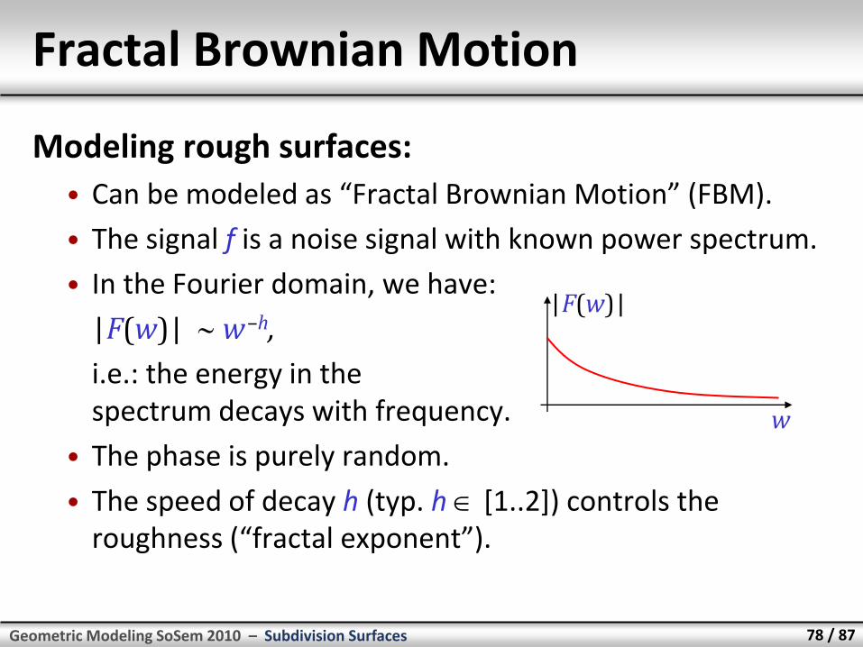
Modeling rough surfaces:
• Can be modeled as “Fractal Brownian Motion” (FBM).
• The signal f is a noise signal with known power spectrum.
• In the Fourier domain, we have:
|F(w)| w –h,
i.e.: the energy in the spectrum decays with frequency.
• The phase is purely random.
• The speed of decay h (typ. h [1..2]) controls the roughness (“fractal exponent”).
w
|F(w)|
Geometric Modeling SoSem 2010 – Subdivision Surfaces 79 / 87
Stochastic Subdivision
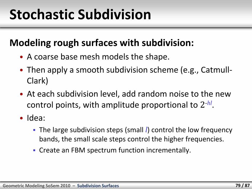
Modeling rough surfaces with subdivision:
• A coarse base mesh models the shape.
• Then apply a smooth subdivision scheme (e.g., Catmull-Clark)
• At each subdivision level, add random noise to the new control points, with amplitude proportional to 2-hl.
• Idea:
The large subdivision steps (small l) control the low frequency bands, the small scale steps control the higher frequencies.
Create an FBM spectrum function incrementally.
Geometric Modeling SoSem 2010 – Subdivision Surfaces 80 / 87
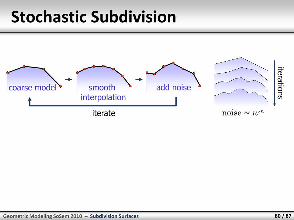
Stochastic Subdivision
coarse model smooth interpolation
add noise
iterate
itera
tions
noise ~ w-h
Geometric Modeling SoSem 2010 – Subdivision Surfaces 81 / 87
Example
Example Application:
• Creating “nice looking” landscapes with “multi-channel fractals”.
• This is rather art than science...
Geometric Modeling SoSem 2010 – Subdivision Surfaces 82 / 87
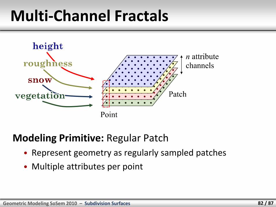
Multi-Channel Fractals
Modeling Primitive: Regular Patch
• Represent geometry as regularly sampled patches
• Multiple attributes per point
Geometric Modeling SoSem 2010 – Subdivision Surfaces 83 / 87
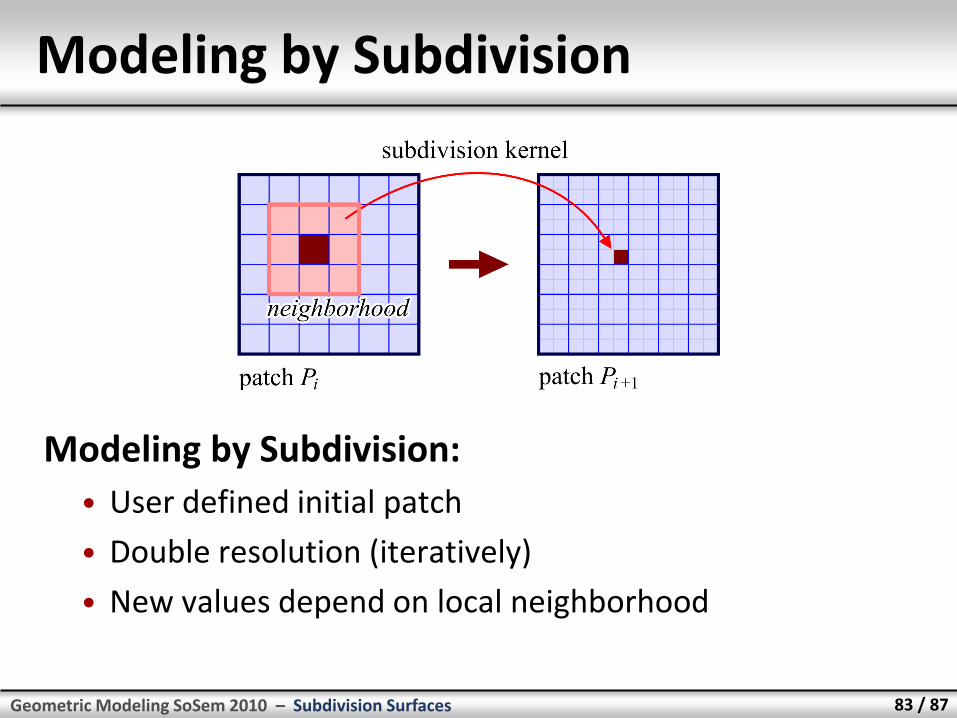
Modeling by Subdivision
Modeling by Subdivision:
• User defined initial patch
• Double resolution (iteratively)
• New values depend on local neighborhood
Geometric Modeling SoSem 2010 – Subdivision Surfaces 84 / 87
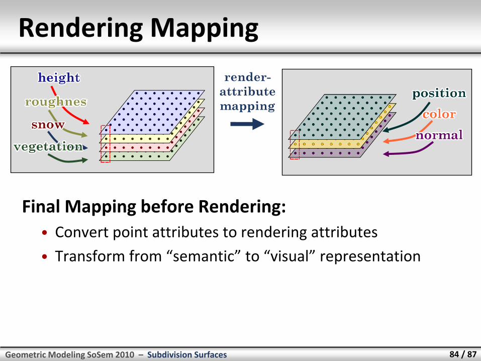
Rendering Mapping
Final Mapping before Rendering:
• Convert point attributes to rendering attributes
• Transform from “semantic” to “visual” representation
render-
attribute
mapping
Geometric Modeling SoSem 2010 – Subdivision Surfaces 85 / 87
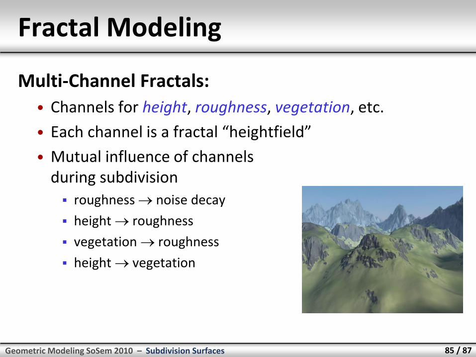
Fractal Modeling
Multi-Channel Fractals:
• Channels for height, roughness, vegetation, etc.
• Each channel is a fractal “heightfield”
• Mutual influence of channels during subdivision
roughness noise decay
height roughness
vegetation roughness
height vegetation
Geometric Modeling SoSem 2010 – Subdivision Surfaces 86 / 87
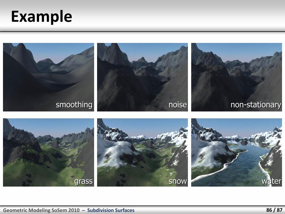
Example
smoothing noise non-stationary
grass snow water