geometry and tensor calculus - home - springer978-94-015-8845-4/1.pdf · 206 geometry and tensor...

Appendix A

Geometry and Tensor Calculus

A.l Literature

There is plenty of introductory literature on differential geometry and tensor calculus. It depends very much on scientific background which of the following references provides the most suitable starting point. The list is merely a suggestion and is not meant to give a complete overview.

• Y. Choquet-Bruhat, C. DeWitt-Morette, and M. Dillard-Bleick, Analysis, Manifolds, and Physics. Part I: Basics [36]: overview of many fundamental notions of analysis, differential calculus, the theory of differentiable manifolds, the theory of distributions, and Morse theory. An excellent summary of standard mathematical techniques of generic applicability. A good reminder for those who have seen some of it already; probably less suited for initiates.

• M. Spivak, Calculus on Manifolds [264]: a condensed introduction to basic geometry. A "black piste" that starts off gently at secondary school level. A good introduction to Spivak's more comprehensive work.

• M. Spivak, Differential Geometry [265]: a standard reference for mathematicians. Arguably a bit of an overkill; however, the first volume contains virtually all tensor calculus one is likely to run into in the image literature for the next decade or so.

• c. W. Misner, K. S. Thome, and J. A. Wheeler, Gravitation: an excellent course in geometry from a physicist's point of view [211]. Intuitive and practical, even if you have not got the slightest interest in gravitation (in which case you may want to skip the second half of the book).

• J. J. Koenderink, Solid Shape [158]: an informal explanation of geometric concepts, helpful in developing a pictorial attitude. The emphasis is on

206 Geometry and Tensor Calculus

understanding geometry. For this reason a useful companion to any tutorial on the subject.

• A P. Lightman, W. H. Press, R. H. Price, and S. A Teukolsky, Problem Book in Relativity and Gravitation [185]: ±500 problems on relativity and gravitation to practice with; a good way to acquire computational skill in geometry.

• M. Friedman, Foundations of Space-Time Theories: Relativistic Physics and Philosophy of Science [92]: a philosophical view on differential geometry and its relation to classical, special relativistic, and general relativistic spacetime theories. Technique is de-emphasized in favour of understanding the role of geometry in physics.

• Other classics: R. Abraham, J. E. Marsden, T. Ratiu, Manifolds, Tensor Analysis, and Applications [1]; V. I. Arnold, Mathematical Methods of Classical Mechanics [6]; M. P. do Carmo, Riemannian Geometry [31] and Differential Geometry of Curves and Surfaces [30]; R. L. Bishop and S. I. Goldberg, Tensor Analysis on Manifolds [18]; H. Flanders, Differential Forms [72].

The next section contains a highly condensed summary of geometric concepts introduced in this book. The reader is referred to the text and to aforementioned literature for detailed explanations.

A.2 Geometric Concepts

A.2.1 Preliminaries

Kronecker symbol or Kronecker tensor:

{ 1 if a=!3 8$ = 0 if a -#!3

Generalised Kronecker or permutation symbols:

( 8~11 ... 88~:'~k' ) =

8~11:::::kk = det: r-

8~; Vk

{ +1 ~ (ILl, ... ,ILk) even permuta~ion of (VI, ... ,Vk) , -1 If (ILl, ... ,ILk) odd permutation of (VI, ... ,Vk) , o otherwise.

Completely antisymmetric symbol in n dimensions:

if (ILl, ... ,ILn) is an even permutation of (1, ... ,n) , if (ILl, ... , ILn) is an odd permutation of (1, ... , n), otherwise.

(A1)

(A2)

(A3)


The tensor product of any two lR-valued operators: if

then

X: DomX -t lR x I--t X(X) ,

Y : Dom Y -t lR : y I--t Y(y) ,

207

(A4)

(AS)

x 0 Y : DomX x Dom Y -t lR : (x; y) I--t X 0 Y(x; y) (A6)

is the operator defined by

x 0 Y(x; y) ~f X(x) . Y(y). (A7)

Alternation or antisymmetrisation of an operator: if

then

AltX: V 0 ... 0 V -t lR: (Xl, ... ,Xk) I--t AltX(Xl, ... ,Xk) ~

k

def 1 '" ( ) = k! L..J sgn 7r X X"'[l] , ... ,X"'[k] , (A9) ".

in which the sum extends over all permutations 7r of (1, ... , k), and in which sgn 7r denotes the sign of 7r. Symmetrisation of an operator: if

then

in which the sum extends over all permutations 7r of (1, ... , k). Index symmetrisation and antisymmetrisation:

X(JL1 ... JLd = ~! L X JLr(l) ... JLr(k) '

".

1 - '" sgn7r X k! L..J 1',,(1) "'JLr(k) •

".

Einstein summation convention in n dimensions: n

Xa ya ~ L:Xaya . a=l

(A 10)

(All)

(A12)

(A13)

(A14)


Einstein summation convention for antisymmetric sums: if XI-'I ... l-'k and YI-'I"'l-'k

are antisymmetric, then

(A.1S) 1-'1 < ... <I-'k

A.2.2 Vectors

A vector lives in a vector (or linear) space:

vEV. (A. 16)

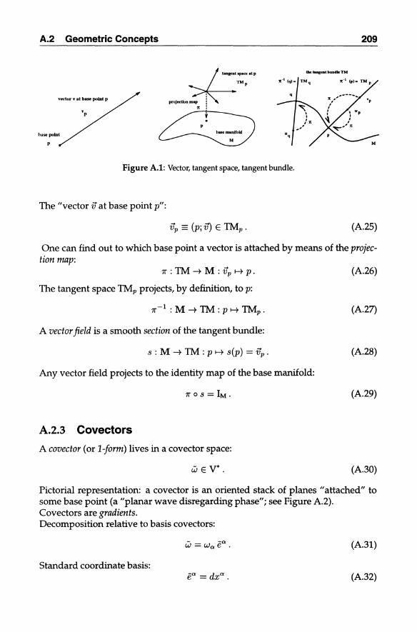
Pictorial representation: a vector is an arrow with its tail attached to some base point (Figure A.l). Vectors are rates: if I is a lR-valued function, then

v[/] = v(df) = dl (v) = va oa/, (A. 1 7)

i.e. the rate of change of I along v (for definition of dl, see Sections A.2.3 and A.2.7). This also shows you how to define polynomials and power series of a vector, e.g.

exp v [I] = f ~Val Oal ... van Oan I . n=O n.

(A.18)

This is just Taylor's expansion at the (implicit) base point to which v is assumed to be attached (see "tangent space"). Leibniz's product rule:

v[/g] = gv[J] + I v[g]. (A.19)

Decomposition relative to basis vectors:

.... a .... V = v ea. (A.20)

Standard coordinate basis: (A.2l)

Operational definition: a vector is a linear, lR-valued function of covectors (or i-forms), producing the contraction of the vector and the covector:

.... V* lR - .... (-) v: -+ :wl-tv w. (A.22)

Often, one attaches a vector space V to each base point p of a manifold M (Figure A.l):

(A.23)

1Mp is the tangent space at p, or the "fibre over p" of the manifold's tangent bundle (Figure A.l):

TM= U IMp. (A.24) pEM

A.2 Geometric Concepts 209

vector y at base point p

?k= ... , ...... ,P

TMp

! proJectIoa map :

" :

hallie point

Figure A.l: Vector, tangent space, tangent bundle.

The "vector vat base point p":

(A.2S)

One can find out to which base point a vector is attached by means of the projection map:

7r : TM ~ M : vp I-t p. (A.26)

The tangent space TMp projects, by definition, to p:

7r-1 : M ~ TM : p I-t TMp. (A.27)

A vector field is a smooth section of the tangent bundle:

s : M ~ TM: p I-t s(p) = vp. (A.28)

Any vector field projects to the identity map of the base manifold:

(A.29)

A.2.3 Covectors

A covector (or 11orm) lives in a covector space:

wE V*. (A.30)

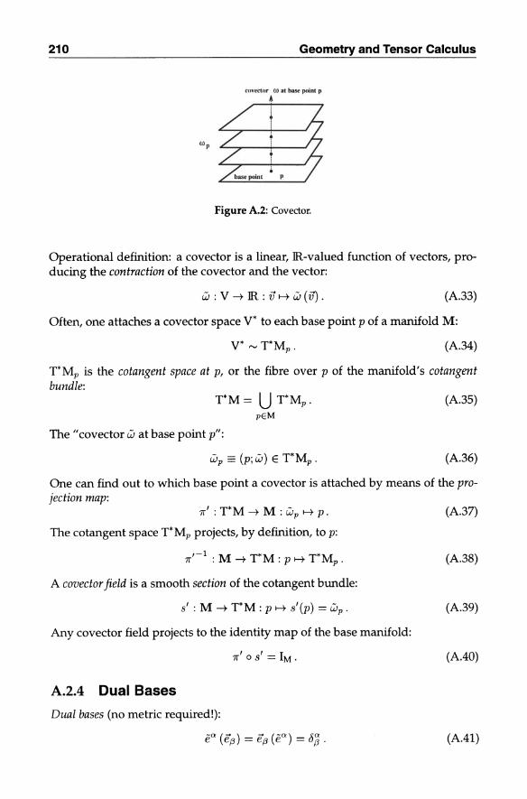
Pictorial representation: a covector is an oriented stack of planes "attached" to some base point (a "planar wave disregarding phase"; see Figure A.2). Covectors are gradients. Decomposition relative to basis covectors:

- -'" w=w",e . (A.31)

Standard coordinate basis: e'" =dx"'. (A.32)


cuudul'" (I) at baR: point p

~

Figure A.2: Covector.

Operational definition: a covector is a linear, IR-valued function of vectors, producing the contraction of the covector and the vector:

w : Y ~ IR : iit--+ w (iJ). (A.33)

Often, one attaches a covector space Y* to each base point p of a manifold M:

Y* "'-'T*Mp. (A.34)

T*Mp is the cotangent space at p, or the fibre over p of the manifold's cotangent bundle:

T*M= U T*Mp. (A.35) pEM

The "covector w at base point p":

(A.36)

One can find out to which base point a covector is attached by means of the projection map:

7r' : T*M ~ M : wp H p.

The cotangent space T*Mp projects, by definition, to p:

7r,-l : M ~ T*M: pH T*Mp.

A covector field is a smooth section of the cotangent bundle:

s' : M ~ T*M: p H s'(p) = wp,

Any covector field projects to the identity map of the base manifold:

7r' 0 s' = 1M.

A.2.4 Dual Bases

Dual bases (no metric required!):

-0< (-) - (-0<) .1:0< e e{3 = e{3 e = U{3 .

(A.37)

(A.38)

(A.39)

(A.40)

(A.41)


.. ~ ..... ,....,.." :

Figure A.3: The gauge figure.

A.2.S Riemannian Metric

Riemannian metric tensor:

G : V x V -+ IR : (v, 'Iii) I-t G( V, w) . (A.42)

A Riemannian metric is a symmetric, bilinear, positive definite, IR-valued mapping of two vectors:

linearity: G('x ii + j.£ v, w) 'xG(17,w) + j.£G(v,w) , = G(v, 17) , symmetry: G( ii, v)

positivity: G( ii, ii) > 0 '</17# o.

The scalar product is another name for the metric:

- - def G(- -) V· W = v,w.

(A.43)

(A.44)

Pictorial representation: a Riemannian metric is a quadric II centred" at some base point, the gauge figure: Figure A.3. The sharp operator converts vectors into covectors:

u V V* - u_defG(- )def -a W : -+ : v I-t w V = V,. = Va e .

The "-operator is invertible, "-1 == " (the flat operator):

L V* V - L - def H( - ) def a-V : -+ : V I-t V V = V,. = V ea ,

with H(" V," W) ~f G(V, W) .

In particular, " converts a basis vector into a corresponding covector:

"ea = ga{3 e{3 .

Similarly, " converts a basis covector into a corresponding vector:

"ea = ga{3 e{3 .

If ea and e{3 are dual, then" e{3 and "ea are dual, too. The "-operator and its inverse motivate the lowering and raising of indices:

..t..: Va = ga{3 vf3 ,

t: va = ga{3 V{3 .

(A.4S)

(A.46)

(A.47)

(A.48)

(A.49)

(A.50)

(A.S1)


Pictorial representation: " (j) represents an inversion in the gauge figure, mapping the tip of a vector to its "polar plane" (vice versa). Equivalent metric representations:

H

1

V* xV* -+ IR

V x V* -+ IR

(ii, 'Iii)

(V, 'Iii)

I-t H( ii, 'Iii) def

I-t I(v, 'Iii)

Decompositions relative to basis:

G ga{j ea ® e{j = "ea ® ea ,

H a{j.... .0...... l -a .0.. .... = 9 e a 'CI e{j = V e 'CI e a ,

1 = 15~ ea ® l[j = ea ® ea .

Corresponding metric components:

G( .... ....) a{j H( -a -(j) ga{j = e a , e{j, 9 = e, e ,

Relation between various metric components:

ap. ~a 9 gp.{j = u{j .

A.2.6 Tensors

(A.S2)

(A.S3)

(A.S4)

(A.SS)

Operational definition: a (mixed) tensor is a multilinear, IR-valued function of vectors and covectors:

T:V® ... ®V®V*® ... ®V* -+IR: ~ --...-.-

k I

(VI, ... , Vk, WI, ... , WI) I-t T( VI, ... , Vk, WI, ... ,wz) .

Decomposition relative to basis vectors and covectors:

T T {jl .. . {jl -al .0.. .0.. -ak .0.......0.. .0.. .... = al ... ak e 'CI ••• 'CI e 'CI e{jl 'CI ••• 'CI e{jl .

Components:

Spivak's convention (tag "5"):

• T is a tensor of type ( 7 ) s·

• T is said to be covariant of rank k and contravariant of rank 1.

Misner, Thorne & Wheeler's convention (tag "MTW"):

• T!; :::e~ are the tensor components of type (i ) M1W (take care!).

(A.S6)

(A.S7)

(A.S8)


• Te;:::~~ are said to be covariant of rank k and contravariant of rank l. • In a space without metric, this terminology carries over to the tensor T itself.

• In a Riemannian space, a tensor can be generalised so as to incorporate "metrical knowledge": see Equation A.68 below.

• If T = Te;:::~~ e{3i ® ... ® e{3/ ® eai ® ... ® eak , its components are written as T{3i ... {3/ ai ... ak' so as to avoid confusion about the ordering of basis vectors and covectors.

Every bundle V gives rise to a tensor bundle:

Dimension:

Special cases:

T E .J~(V).

dim .J~ (V) = n HI .

= .J? (V) ("contravariant tensors of rank l") ,

.J~ (V) ("covariant tensors of rank k") .

(A.59)

(A.60)

(A.61)

(A.62)

A tensor bundle, generalising a vector or covector bundle, comprises fibres and base points:

.J~(1M) = U .J~(1Mp). (A.63) pEM

The base point of a tensor is revealed by the projection map:

II : .J~(1M) -+ M : Tp f-t p. (A.64)

The fibre .J~(1Mp) projects, by definition, to p:

(A.65)

A tensor field is a smooth section of a tensor bundle:

~ : M -+ .J~(1M) : p f-t ~(p) = Tp. (A.66)

Any tensor field projects to the identity map of the base manifold:

(A.67)

In a Riemannian space, a tensor can be generalised so as to incorporate built-in conversion rules based on the H and ii-operators:

T '" {T; H, iI } (A.68)

having the following interpretation:


• T E :1~ (TM) is any "prototype tensor" of fixed total rank k + I as defined above.

• The cast operator" (or its inverse, b) is implicitly invoked whenever an argument (a vector or covector) passed into a slot of T does not match the prototype T.

• The type of T is characterised by its total rank m = k + I.

• The partial, covariant and contravariant ranks k and l refer to any representative prototype T (and its components) used in a particular "realization" T ofT.

The "-operator can be used to convert between different representations of a rankm tensorT:

T E :1~ (V) ~ T' E :1f,' (V) with k' + I' = k + l = m . (A.69)

In particular, you can define t T E :1i (V) by applying" and b to all basis vectors and forms in the decomposition of T (component representation: raising all lower and lowering all upper indices). You may similarly define + T E :1k+1 (V) and tT E :1 HI (V) by applying only" or b to either basis vectors or covectors. The norm of a tensor: ifT E :1~(V), thentT E :1i(V), so you can "contractT onto itself" to get its squared norm:

II T 112 ~tT(T) =tT(+ T) . (A.70)

Components:

li T 112 - T 1'/+1···1'1<+1 TI'1 ... 1'1 - TI'1 ... l'k+1 T - 1'1···1'1 1'1+1···l'k+1 - 1'1···l'k+1 . (A.71)

But: see also Equation A.88 below. Example of T '" {Tj U , b }: the metric tensor G : V x V -+ R as defined previously (A.42-A.43) is a prototype for the generalised metric tensor G; depending on what you feed it, G behaves either as the prototype G (2 vectors), H (2 covectors), or I (1 vector and 1 covector, respectively).

Tensors of the same type ( ! ) M1W = (~ ) 5 can be linearly combined:

(>. S + JL T)(Vl,".' Vk,Wl, ... ,WI) = >. S( VI, ... , Vk, WI, ... , WI) + JL T( VI, ... , Vk, WI, ... , WI) . (A.72)

Tensors of arbitrary types ( ~ ) M1W and ( ;;. ) M1W can be multiplied; if

Vk == (VI, ... ,Vk), Wm == (uh, ... ,Wm), 01 == (WI,.'. ,WI), En == (Ul, ... ,Un) (A. 73)

then (A.74)


yielding a product tensor of type ( ~ !;::, ) MlW'

Symmetrising tensors: if S E .:Jk(V), then

SymS E ~k(V).

Components:

215

(A.7S)

(A. 76)

Similar definitions apply to contravariant and mixed tensors (symmetrisation of mixed tensors is carried out as an independent symmetrisation of covariant and/ or contravariant parts): if T E .:Jl (V) and U E .:J7 (V), then

Sym T E ~1(V»)

Sym U E ~7(V).

Alternating or antisymmetrising tensors: if S E .:Jk(V), then

AltS E Ak(V).

Components:

(A. 77)

(A.78)

(A. 79)

(A.80)

Similar definitions apply to contravariant and mixed tensors (alternation of mixed tensors is carried out as an independent alternation of covariant and contravariant parts): if T E .:Jl(V) and U E .:J7(V), then

AltT E A1(V»)

AltU E A7(V).

The Alt -operator is idempotent:

Alt 0 Alt = AU .

(A.81)

(A.82)

(A.83)

The Alt -operator is linear, hence can be viewed as a constant tensor. When acting on a rank-k cotensor S with components S!-'l ... /J-k/ Alt has components

(A.84)

Decomposition relative to basis: if SEA k (V), then

(A.8S)

with S!-'l"'!-'k = S[!-'l ... !-'k] antisymmetric; see also Equation A.93 below. Similar definitions apply to the alternation of contratensors and mixed tensors (the latter corresponding to the tensor product of two permutation tensors). The wedge product is an antisymmetrised tensor product: if Si E A ki (V) then

(A. 86)


Components: if K,j = 'Li=1 ki' then

(A.87)

Rule of thumb: 51/\ ... /\ Sp equals 51 0 ... 0 Sp plus terms that guarantee complete antisymmetry. Likewise for Si E Ak; (V). In the general case of mixed tensors you are supposed to "wedge" the covariant and contravariant parts independently. Special cases: k-forms and k-vectors: if WI, ... ,Wk and VI, ... ,Vk are k covectors and k vectors, respectively, then Wl/\ . . . /\Wk E A k (V) is a k-form, and Vl/\ . .. /\ Vk E

Ak (V) is a k-vector. When defining the norm of an antisymmetric tensor one often incorporates a combinatorial factor to avoid "overcounting": if A is an antisymmetric tensor of rank k (typically prototyped by some k-form A E A k (V) or k-vector A E Ak (V), then

II A 112 = AI I A/'l ... /'k /'1·· -/'k

Physical interpretations of n-forms and n-vectors (in n dimensions):

• n-forms are densities;

• n-vectors are capacities.

Basis k10rms: the set of all

is a basis for A k (V). Basis k-vectors: the set of all

is a basis for Ak(V). Consequently:

dim Ak(V) = dim Ak(V) = (~ ) .

A unit k-form is designed to exactly fit its dual unit k-vector:

e/'l /\ ... /\ e/'k (eV1 /\ ... /\ eVk ) = eV1 /\ ... /\ eVk (e/'l /\ ... /\ e/,k) = t5~ll:::::kk .

(A.88)

(A.89)

(A.90)

(A.91)

(A.92)

It is more natural to use the wedge product basis than the ordinary tensor product basis for decomposing an antisymmetric tensor: if 5 E A k (V), then

(A.93)

Reminder: tensor coefficients S 1'1. _ -/'k are usually defined in terms of the ordinary tensor product basis. The Levi-Civita tensor in n dimensions is the unique unit n-form of positive orientation:

def r;:; -1 -n -/'1 -/' C = v g e /\ ... /\ e = C /'l ... /'n e /\ ... /\ en, (A.94)


'th def d WI 9 = etgij' Covariant and contravariant components:

217

(A.95)

(A.96)

The Hodge star operator converts k-forms (k-vectors) into (n - k)-forms «n - k)vectors, respectively):

(A.97)

It can be defined recursively: if SEA k (V) is a k-form and W E A I (V) is a I-form, then

In general, if

then

where

A.2.7 Push Forward, Pull Back, Derivative Map

Push forward and pull back:

{ f* : V -t W 1* : W* -t V* ,

in which f* is any linear map and

for all V' E V and W E W* ,

Diagrammatically:

J*WET*M ~ WET*N

1 1 1*w (V')

(A.98)

(A.99)

(A.IOO)

(A.101)

(A.I02)

(A.I03)

(A. 104)


In general you can pull back any kind of tensors:

(A 105)

with, by definition,

f*T(ih, ... , Vk) = T(f*(vd,···, f*(Vk)) for all VI, ... , Vk E V and T E :rk(W). (Al06)

Typically, any function on a manifold f : M -+ N induces a linear map, its differential:

(A 107)

The differential gives you the difference between "tip and tail" of a vector (see Section A2.2):

df (v) = vU]· (Al08)

Decomposition relative to coordinate basis:

df = 8/l-fdx/l-. (Al09)

Commutative diagram:

TM~TN (All0)

M~N The chain rule,

d(g 0 f)(p) = dg(f(p)) 0 df(p) , (Alll)

can be restated as (A112)

AppendixB

The Filters ~PI ... Pl ILl·· ·ILk

Consider the first case of Result 6.1, Page 184. Using the following lemma we can get rid of the derivative 01-' in the integrand (we use Cartesian coordinates).

LemmaB.l Using parentheses to denote index symmetrisation, we have

° q;PI···PI (x) = _q;PI···PI (x) + 6 (PI q;PI ... PI-t) (x) . I-' I-'l···/Lr. /LI···/Lr./L /L I-'l···/Lr.

It is understood that q;~~ '::.~; I == 0 if I = o. The proof of this lemma is straightforward and will be omitted. Using this lemma we can rewrite Result 6.1:

ResultB.l See Result 6.1.

M

01-'1 ... /Lr.£VM F[<p] = L V~;PI"'PI !dX f(x) [q;~~·::.~r./L(x) - q;~~'::.~;l (x) 6~'] . 1=0

(Note that index symmetrisation w.r.t. PI, ... ,PI is automatic by virtue of symmetry of the coefficients V~;PI"'PI.) One may compare this result to the second case of Result 6.1.

The essence is now to express the overcomplete set of filters q;~; .. ::~r. in terms of Gaussian derivative filters <P/LI .•• /L .... Consider the following diagram.

q;PI ... PI (x) F ~PI ... PI (w) /LI· .. /Lr. ---+ /LI···I-'r.

*1 1 ** q;PI···PI (x)

Finv ~PI"'PI (w)

/LI·· ./Lr. +--- /LI·· ./Lr.

Instead of simplifying directly in the spatial domain (the arrow marked by a * indicates a simplification step), we take the Fourier route (F --+ ** --+ F inv), and

220 The Filters ipPl .. ·PI /L1 •.. f.J,k

simplify in Fourier space. According to Definition 2.8, we can make the following formal identifications of operators (the l.h.s. in the spatial domain, the r.h.s. in the Fourier domain):

P . 8 x == Z 8wp ,

We need one more definition.

Definition B.l (Hermite Polynomials)

8 . -8 == zWp. xP

The Hermite polynomial of order k, Hb is defined by

dk 12k 1 2 - e-2"X = (-1) Hdx) e-2"x dx k

(B.l)

This is appropriate for the I-dimensional case. Let us define the n-dimensional analogue of the Hermite polynomials as follows.

Definition B.2 (Hermite Polynomials in n Dimensions) The n-dimensional Hermite polynomial of order k, 1lil ..• ik , is defined by

These n-dimensional Hermite polynomials are related to the standard ones in the following way.

Lemma B.2 (Relation to Standard Definition) The n-dimensional Hermite polynomials as defined according to Definition B.2 are related to the standard definition, Definition B.1, as follows.

n

1lil ... ik(X) = II Ho/1 ... ik(Xj ) ,

j=l J

in which at·· iA, denotes the number of indices in i 1 , ... , ik equal to j.

Clearly we have 2:]=1 a? ... ik = k, since this simply sums up all indices. The separability property of Lemma B.2 follows straightforwardly from Definition B.l, when applied to a multidimensional Gaussian.

Having established all basic ingredients and notational matters, we can now relate the overcomplete family of filters ip~~'::'~k to the Gaussian family. This is easy, since all we need to do is to use Leibniz's product rule for differentiation in

fi..Pl"'PI ( ) _ (_l)k.~ .~ (. . 1()) "±"l'l"'l'k W - II Z 8w ... z 8w zW/l l •· .zw/lk'f' W ,

. Pl PI (B.2)

(see Formula B.1 and the definition of the filters in Result 6.1). Then, each time we have to take a derivative of 4>(w), we use the explicit property of the Gaussian stated in Definition B.2. In this way we arrive at

The Filters cpP1 .. 'Pl 1L1 ... lLk 221

Result B.2 (The Filters Cp~~·::.Vk and the Gaussian Family) Let S denote the index symmetrisation operator (applying separately to upper and lower indices), then we have

<l>P1 ... PI (w) = /L1···/Lk

(_I)k S {m~.1) ( 1 ) (-I)mk! <P1 <Pm' . (.)I-m'1JPm+1"'PI( )J..( )} -l-! - ~ m (k _ m)!O/L1 '" 0/L", tW/Lm+1 ... ZW/Lk -z n. W 'f' W •

Fourier inversion yields

<l>~i·::.~lk (x) =

(_l)k S {m~'I) ( 1 ) (-Irk! <P1 <p", a a .1-m'1JP"'+l ... PI(''<"7)A..()} -l!- ~ m (k _ m)!o/L1" .o/L", /L",+1'" /Lk Z n. Z v 'f' X •

Note that this expression is real in the spatial domain, since i P1-lP1 ••• Pp (i V) is a real differential operator for any p E zt. To see this, look at the explicit form of a Hermite polynomial:

(B.3)

in which [x 1 denotes the entier of x E JR., i.e. the largest integer less than or equal to x, and in which the double factorial (2m - I)!! indicates the product 1 x 3 x .,. x (2m - 1). Consequently,

.k .~ __ k [k/2] ( k) _" dk- 2m Z Hk(Z dx) - ( 1) ~ 2m (2m 1) .. dxk-2m ' (BA)

very real indeed. The general n-dimensional case follows from this observation. Note also that the r.h.s. of Result B.2 is a linear combination of Gaussian derivatives of the type <PJ.L1 ... J.L,,' with p = 0, ... , k + l. Thus we have indeed proven overcompleteness of the (apparently (k + l)-th order) filters Cp~~'::,Vk by explicitly rewriting them in terms of Gaussian derivatives.

Appendix C

Proof of Proposition 5.4

To proof Proposition 5.4 we embed the k x k matrix A~;·::.~kk' introduced in Defini

tion 5.8, into a d x d-matrix A~;'::'~k' which has the same determinant, by adding a (d - k) x (d - k) identity block, as follows:

A""" ·"'k = -::-....<:..1..:..: .. "". =--1-,..-";";';';"-"--'-"-_ ( AV1"''''k

1-'1"'1-'1. O(d-k)Xk

We can write the determinant of the matrix A~~·::.~kk with the use of a double g

product:

Despite its d2d terms, this is actually a rather sparse sum: only those terms for which the indices (Q:1, ... , Q:d) and ((31, ... , (3d) are permutations of (1, ... , d) survive, and we may reorder them in such a way that the first k indices address the actual matrix elements of A~~·::.~~. To this end we consider all permutations (k1, ... ,kd) of (l, ... ,d), such that the k-tuple (Q:kl' ... ,Q:kk) and the (d - k)tuple (Q:kk+l'''' Q:kd) are permutations of (1, ... , k) and (k + 1, ... , d), respectively. If we take into account a combinatorial factor, counting the various possibilities to choose this separation, we may assume that the indices Q:k" ... , Q:k k

and (3k" ... , (3kk index the actual matrix elements of the block A~~·::.';:k' whereas Q:kH1' ... , Q:kd and (3kk+1 , ... , (3kd index the identity block. In other words,

for the first k subindices i = 1, ... , k, and

for the last d - k indices i = k + 1, ... , d. This leads to the following expression:

det A""''''''k - - c C k1'" kd /j '1 /j k /j k+1 /j'd - ( d) 1 (3 (3 "'''k "'''k O<k O<k 1-'1 .. ·l-'k - k d! O<k, .. ·O<kd iLf3k1 ••• iLf3kk (3kk+1'" (3k d '

224 Proof of Proposition 5.4

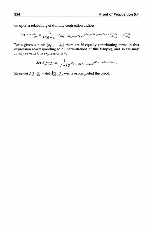
or, upon a relabelling of dummy contraction indices:

For a given k-tuple (ki , . .. ,kk) there are k! equally contributing terms in this expression (corresponding to all permutations of this k-tuple), and so we may finally rewrite this expression into:

Since det AV1 ••• V k = det AV1 ... Vk we have completed the proof. 11-1·· ·l1-k 11-1· •• l1-k'

AppendixD

Proof of Proposition 5.5

Write {L,So, ... ,Sd-l,h, ... ,Id}, with Sk = LilLili2Li2i3 ... Likik+1Lik+l (k = 0,1,2, ... ) and h = Lili2Li2i3 ... L iki1 (k = 1,2,3, ... ; both Sk and h contain k 2-vertices), and observe that all connected polynomial diagrams are of the form L, Sk or h+1 for some k ~ O.

We will first consider a system with 2-vertices only, and show that all Ik for k > d are reducible. Then we will tum to the general case, first by including the Sk, showing their reducibility for k > d - 1, and then by extending it with the trivial zeroth order member L.

0.1 Irreducible System for {Lij} We concentrate on the second order system {Lij }.

Definition D.l Recall Definition 5.8, and define

L~~] ~ 8il ... iki;jl ... jdLidl··· L ikjk ,

X[k] ~ 8il ... ik;Jt ... jkLidl'" Lidk .

By developing the (k + 1) x (k + 1 )-determinant underlying the generalised Kronecker tensor of rank k + 1 in the definition of L~~] w.r.t. the last column into k x k-determinants one may derive the following identity:

(D.l)

(D.2)

226 Proof of Proposition 5.5

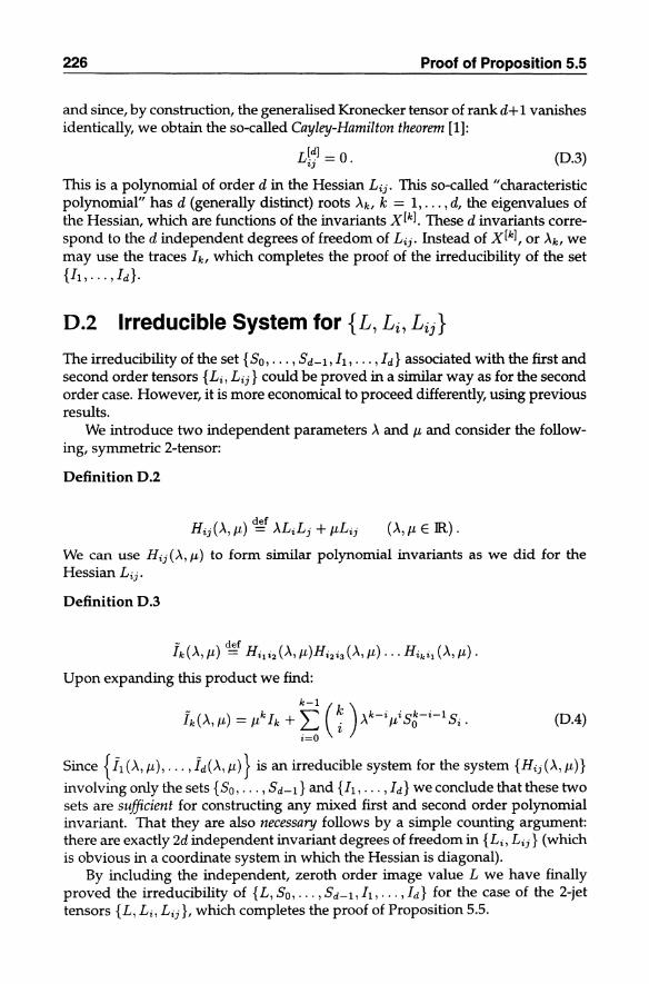
and since, by construction, the generalised Kronecker tensor of rank d+ 1 vanishes identically, we obtain the so-called Cayley-Hamilton theorem [1]:

(D.3)

This is a polynomial of order d in the Hessian Lij . This so-called "characteristic polynomial" has d (generally distinct) roots >'k, k = 1, ... , d, the eigenvalues of the Hessian, which are functions of the invariants Xlkl. These d invariants correspond to the d independent degrees of freedom of Lij. Instead of Xlkl, or >'k, we may use the traces Ik, which completes the proof of the irreducibility of the set {h, ... ,Id}.

D.2 Irreducible System for {L, Li , Lij}

The irreducibility of the set {So, . .. , Sd-b II, ... , Id} associated with the first and second order tensors {Li, Lij} could be proved in a similar way as for the second order case. However, it is more economical to proceed differently, using previous results.

We introduce two independent parameters>. and JL and consider the following, symmetric 2-tensor:

Definition 0.2

(>., JL E IR) .

We can use Hij(>', JL) to form similar polynomial invariants as we did for the Hessian Lij .

Definition 0.3

- def Ik (>., JL) = Hil i2 (>., JL )Hi2i3 (>., JL) ••. Hikil (>., JL) •

Upon expanding this product we find:

1-(') kI ~ (k) ,k-i iSk-i- IS k 1\, JL = JL k + to' i 1\ JL a i . (D.4)

Since {II (>., JL)' •.• ,id(>', JL) } is an irreducible system for the system {Hij(>', JL)}

involving only the sets {So, ... , Sd-l} and {h, ... , Id} we conclude that these two sets are sufficient for constructing any mixed first and second order polynomial invariant. That they are also necessary follows by a simple counting argument: there are exactly 2d independent invariant degrees of freedom in {Li , Lij} (which is obvious in a coordinate system in which the Hessian is diagonal).

By including the independent, zeroth order image value L we have finally proved the irreducibility of {L, So, . .. , Sd-l,!l, ... ,Id} for the case of the 2-jet tensors {L, Li, Lij }, which completes the proof of Proposition 5.5.

Solutions to Problems

Solution2.2. F E S'(IRn)iscontinuous: iflimk-+oo </>k = </> inS(IRn), thenlimk-+oo F[</>k) = F[</». The claim that S(IRn) has "a very strong topology" means that the construction of a convergent sequence in S (IR n) is a very hard job. Once you have accomplished that it will be difficult to construct a linear map that does not converge (in the usual sense of convergence in IR as explained above). Continuity is desirable in the context of measurements, because it is a necessary condition for stability.

This suggests that, in order to construct a discontinuous functional, one has to weaken the topology. Here is an example of a discontinuous functional from Rudin's book on functional analysis [246, Chapter 1, Exercise 13]. Let C be the vector space of all complex functions on [0, 1). Let (C, 0-) be C with the topology induced by the metric

11 If(x) - g(x}l d(f,g) = 0 dx 1 + If(x) - g(x)I'

Moreover, let (C, T) be the topological vector space defined by the seminorms

Px(f) = If(x)1

Then the identity operator from (C, T) to (C, 0-) fails to be continuous.

Solution 2.3.

a. We have (in n dimensions)

ftlx-all<O' dx {¢(a) + O(lIx - all)} n XJ3(a·O'Ml = r = </>(a) + 0(0- ),

, Jllx_all<O'dx

for all </> E S(IRn ), so that limO'.).o XJ3(a;O') = oa.

b. Note thatthe integral of,a;O' depends neither on a nor on 0-. Define,(x) = 'a=O;O'=I(X). The standard integral

jdX,(x) = 1

can be easily proven for n = 2 using polar coordinates, and from there for any n E Z+ by virtue of separability.

228 Solutions to Problems

c. Directly in the spatial domain we can switch from "pull back" to "push forward" representation, as follows. Reparametrise x = a + u(. and define ¢>a;u((.) = ¢>(a + u(.), then

lim "Ya'u [¢» = lim "Y[¢>a'u) = "Ynim ¢>a·u) = ¢>(a) , u.j.o' u.j.O ' l~.j.o'

in which we have made use of the previous result. This holds for all ¢> E S(1Rn ), in other words, limu.j.o "Ya;u = 8a. Alternatively one can look at the Fourier representation of the function "Ya;u(x):

~ () iaw_ 1 (72w 2 "Ya;u w = e 2 ,

which in the limit of vanishing scale becomes eiaw = 8a (w).

Solution 2.4.

a. Plain substitution; note that you can put a = 0 by virtue of shift invariance.

b. The r.h.s. satisfies the diffusion equation and has the right limit for u .1. 0; since the solution in S(1Rn) is unique, it must be another notation for the l.h.s.

See also Solution 2.12.

Solution 2.5.

a. H E S'(lR) because H[¢» ~f fo"" dx¢>(x) is always well-defined and continuous if ¢> E S(lR).

H'[¢» ~f - fo"" dx¢>'(x) = - [¢>(x»):::o"" = ¢>(O) = 8[¢», so H' = 8.

b. Ixl [¢» ~f f dx Ixl ¢>(x) = - f~"" dx x ¢>(x) + fo"" dx x ¢>(x), both terms are well-defined and well-behaved if ¢> E S(lR).

Ixl'[¢» ~ -fdxlxl¢>'(x) = f~""dxx¢>'(x)-fo""dxx¢>'(x)~' -f~oodx¢>(x)+ fooo dx ¢>(x) = f dx [H(x) - H( -x») ¢>(x), whence lxi' = sgn (x).

Similarly, Ixl"[¢» clef -lxl'W) = -fdx[H(x)-H(-x»)¢>'(X) p~. f dx [H'(x) + H'( -X») ¢>(X) = f dx [8(x) + 8( -X») ¢>(X) = 28[¢», SO Ixl" = 28(x).

Solution 2.6.

a. First observation: ¢>(x) ~ m! xm for all x E lR and m E llt; this follows from the series expansion of the exponential (consider the expansion of 1/¢>(u) in terms of u = l/x). Secondly, it follows by induction that the k-th order derivative is of the form ¢>(k l (x) = Pk(l/x) ¢>(x), in whichpk(u) is a (2k)-th order polynomial. This implies that there exists a constant Mk such that IPk(u)1 ~ Mk u2k if u ~ 1, which in turn implies that¢>{kl(x) ~ Mkm!xm-2k. We are free to choose m > 2k,sothatwemusthave ¢> E Ck(lR), and ¢>(kl(O) = O.

h. In ID you can take 1/>I(X) = ¢>(x - a) ¢>(b - x); in nD, "Ij1,,(x1, ... , x") = rr=l "Ij11(Xi ).

c. By smoothness and compact support there exists a point Xo E lR where all derivatives vanish, a{k l (xo) = 0 for all k E llt. By analyticity we have a convergent Taylor series

_(k){~~\ a(x) = L:;;"=o ~(x - XO)k = 0 for all x E lR.

Solutions to Problems 229

Solution 2.S.

a. Take n, a = 1, the general case is straightforward. Conventional differentiation is defined for the subclass f E C1(ffi.) n P(ffi.) C S'(ffi.), in which case we have

-F[4>'J ~f - f dx f(x) 4>'(x) p~. f dx J'(x) 4>(x) - [J(x) 4>(x)J:~~:. The boundary term vanishes by construction of S(ffi.), and the remainder equals F'[4>J, in which F' is the RTD corresponding to the classical derivative J' (x). Moreover, if F' [4>J = G[4>J for some RTD G corresponding to a function 9 E CO (ffi.) n P(ffi.), then, by a claim somewhere after Definition 2.12, J' = g, so in the appropriate subspace the RTD F' and the classical function J' are one-to-one related.

b. From partial integration in the appropriate subspace it follows that '\7 t = -'\7. From the definition of the complex scalar product (cf. Problem 2.10) it follows that ct = c· for any complex multiplier c E <C. For any two-not necessarily commuting-linear operators A and B we have (AB)t = Bt At (this follows immediately from the defini-

tion of conjugation, A tv· W ~f v· Aw, a "last-in first-out" process). Minus signs cancel: (i'\7) t = '\7 t it = (-i)( - '\7) = i'\7.

c. By the same token we have pt ('\, '\7) = (Llol$m '\0 (x) '\7 0 r = LlolSm (-1)1"'1'\7 '" 0

,\~ (x). Note the reversed order of operators!

d. The eigenvalue equation for eigenvalue w is i'\74> = w4>, a nonzero solution of which exists for all w E ffi., given by 4>",(x) = e- i ",,,, up to arbitrary normalisation. In other words, the eigenvalue spectrum is just the Fourier frequency spectrum, while the corresponding eigenvectors correspond to the Fourier basis of planar waves.

Solution 3.2.

a. Note that the base point is 7r"'[4>a;AJ = a"'. The rest follows from shift invariance of the Lebesgue measure dx = d(x - a); the integrand depends only on x-a.

b. Results: O"O[4>a,AJ = I (by filter normalisation), O"f[4>a,AJ = 0 (by definition of central momenta), O"~V[4>a,AJ = A"'v. The nontrivial ones are easily computed in a Cartesian frame by reparametrising x = ~, in which R is a rotation matrix such that RT A -1 R = diag {sI1, . .. ,S;;-I}, after putting a = O.

c. The case for odd orders 2k + 1 follows from anti-symmetry of the integrand. The expression given for even orders should be obvious from the definition of momenta (each '\-derivative brings in a factor x 2 ).

d. If we introduce the symbol a'? ···"'k that counts the number of indices among the 1-£1, ••• ,I-£k that equal j, then we can factorise the n-dimensional momentum into n I-dimensional momenta:

Note that L7=1 ajl ... "'k = k, because this is just the total number of indices. Consequently all we need to do is evaluate the I-dimensional momenta 0" ","'l···"'k [4>a;;.,.2J for

J J

each dimension j. From the previous representation we conclude that

["- J-(-2 2)k{~_I_} -(2k-I)1I 2k 0"2k 'l'a;.,.2 - 0" d,\k,f). ).=1 - .. 0".


Solution 3.4. For O{x) = Mx + a we get O.4>{x) = I detMinv l4>{MinV{x - a», which is identical to the Gaussian of Problem 3.2 if we take A = M MT. Note that this is always possible by the constraints on A, and in particular that I det MI = v'det A.

Solution 3.S.

a. (." 0 0).4> = J('109 )inv4> 0 (." 0 O)inv = J'1inV (J9inv 4> 0 omV) o."inv = (.". 0 0.)4>. From this it follows that for all admissible 4>, (." 0 0)· F[4>1 = F[(." 0 0).4>1 = F[(.". 0 0.)4>1 = .". F[O.4>1 = (0· o.,,·)F[4>I.

b . .". F[O.4>1 = F[(." 0 0).4>1 = F[id.4>l = F[4>I· c. f'(y) =.". fey) = f(.,,(y» = f(x).

d. 4>'(y) = o.4>(y) = J'1(Y) 4> (." (y» = Idet ~;I4>(x).

e. By substitution of variables x = .,,(y) we can rewrite >.' = F'I4>'I = f dy !' (y) 4>' (y) = fdYldet~(y)lf("'(Y»4>("'(Y» = fdx f(x) 4>(x) = F[4>1 = >., showing the parametrisation independence of a local sample.

Solution 3.7.

a. One has ten - l)(n - 2) Euler angles for rotations, 2 scale parameters, n shift parameters, and n - 1 velocity parameters.

b. Subtract n - 1 from the previous count.

c. One has td(d - 1) Euler angles for rotations, but this time only 1 scale parameter and d shift parameters; in addition one has d velocity parameters when adding Galilean boosts.

Solution 3.S. The eigenvalues>. are the solutions of det(X - >.1) = (1 - >.t = O. Apparently we have only a single eigenvalue A = 1, independent of v. Eigenvectors are the nontrivial elements of the null space of X - >.1, which is of dimension (n - 1), spanned by thebasis vectors ei = (OJ ei), where ei is the standard basis vector with components e~ = cSt, i, j = 1, ... , n - 1.

Solution 3.9. If we transform all M quantities Xi -t >."'i Xi (i = 1, ... , M) under a rescaling of a single hidden scale parameter, then F(Xl, ... , XM) = 0 will be recasted into F(>''''lXl, .•. , >."'M XM) = O. Differentiation w.r.t. >. at >. = 1 yields the I-st order p.d.e. QIXI :~ + '" + QMXM o~: = O. For N independent hidden scale parameters labelled by an index I' = 1, ... , N we thus get N such equations in N independent scale parameters Ap., and we likewise obtain a system of N p.d.e.'s by differentiation:

OF OF - 0 Qp.lXla"'l + ... + Qp.MXM a"'M - .

Solution 3.10.

a. For 0", : z t-+ z + X we get O;f{z) = fez + x) and consequently O;F[4>1 = f dz fez + x) 4>{z) = F * 4>{x). e· F is symbolic notation for the entire collection {O· FlO E e}, i.e. we can identify e;F with the "function-valued" distribution F*, with independent variable x.

b. Differentiation commutes with translation: V 0 0", = 0", 0 V. Therefore V",F * 4> = V",8· F[4>1 = e· V", F[4>1 = e· F[Vd4>1 = F * Vd4>. The equality V",F * 4> = F * V", 4> follows directly from the two equivalent integral representations for F * 4>: f dz fez) 4>(x - z) = f dz f(x - z) 4>(z), or, less sloppy, by noting that F * 4> = F * ~ (where ~(x) = 4>(-x».


Solution 3.13.

a. A is, by definition, a linear space, so we can add and scalar-multiply filters in the proper way, and in addition we have the * operation, which satisfies all criteria of Equations 3.2 and 3.5.

b. This is Lemma 2.1. We can rewrite x"'V' p(1) * .,p)(x), using x'" = E"Y$'" ( ~ ) (x -

y)"'-"Yy"Y, as E"Y$'" ( ~ ) (x"'-"Y1»*(x"Y V' p.,p), whichisa finite sum of convolution prod

ucts, in each term of which one of the factors is integrable, and the other one bounded. Integrability and boundedness of the two respective factors in a convolution product suffice to make it bounded. Thus x'" V' p (1) * .,p)( x) is bounded for all multi-indices a and (3, in other words, 1> * .,p E S(IRn).

c. There is no identity element in S(IRn), and one cannot invert the filters. Convolution is commutative (abelian).

Solution 3.19. Since m2[1>t] = 0 for a > 2, these cases cannot correspond to positive filters. For a =f. 2 the momenta do not all exist, hence the filter cannot be in S(IR) (recall that spatial momenta correspond to derivatives at zero frequency in Fourier space).

Solution 3.23.

a. Nt = (At A) t = (At A) = N. This implies that N has only real eigenvalues, and an orthonormal basis of associated eigenfunctions. For any .,p we have .,p . N.,p = II A.,p 112 ~ O. In particular, if.,p is itself a normalised eigenfunction (.,p . .,p = 1) with eigenvalue A, then A =.,p. N.,p ~ O.

b. This follows from [ te ' ~] = 1.

c. By induction we find [A, Atk+!] = Atk [A, At] + [A, Atk] At = (k + 1) Atk, in which we have used the previous result. For a general, analytical function f, we can use its Ta~lor series expansion in combination with the present result to find [A, f(A t)] = f'(A ).

d. Let.,po be the normalised eigenfunction corresponding to the smallest eigenvalue no, II.,poIl2 = 1. NotingthatN = AAL 1,wegetNA.,po = A (AtA-1).,po = (no-1)A.,po. However, no - 1 cannot be an eigenvalue, so A.,po = O. Furthermore we obtain no = .,po' N.,po = IIA.,po112 = o.

e. Once we have solved for the initial eigenfunction .,po, we can create a sequence of eigenfunctions by successive application of At. To see this, note that .,p" is indeed an eigenfunction of N with eigenvalue k, because N.,p" = AAt(*,At".,po) = *,([A,At"] + AtA).,po = k.,po. Using.,p" = 7,:At.,p"-l we see that it is also normalised: iIIAt.,pk_11l2 = t.,p"-l . (N + 1).,p"-1 = 1 (last step by induction).

f. H=N+ ~I. g. This should be evident from the previous results.

h. We only prove orthonormality. Assume l ~ k, and evaluate .,pk . .,p, with the help of d and e: .,p" . .,p, = VW.,po· A'-".,po = 8",. The notation for completeness is explained as follows: for any f(x) we can make the eigenfunction decomposition

f(x) = EkEZt f . .,p" .,p,,(x) = J dy {E"EZt .,p,,(x).,p,,(y)} f(y). Thus we can make

the identification E"EZ+ .,p,,(x).,p,,(y) = 8(x - y). o


i. Left to the reader (separation of variables).

Solution 4.3. If the orders in a term J dx .p(j)(x) .p(kl(x) add up to an odd integer, say j + k = 2i + 1, then repeated partial integration can be used to cast it into the form (_I)i Jdx.p(il(x).p(i+l l (x). Thus the integrand is a total derivative, so that the integral vanishes by virtue of rapid decay. Otherwise, if the orders add up to an even integer, say j + k = 2i, then terms can be put in the form (_I)i J dx .p(il(x) .p(il(x) by the same trick.

Solution 4.7. Consider the gradient of the second order scale-space polynomial,

{ L",(x,y) Ly(x, y)

= Lx + Lxx x + Lxy y Ly + L",y x + Lyy y .

Disregard all pixels except candidates that might be hiding critical points, i.e. pixels at which we measure 0 S L; + L; S E2 M2, in which EM is a suitable threshold for the gradient magnitude. If M is the average or maximum gradient magnitude in the image, we may assume that 0 < E ~ 1 and make a perturbation expansion to find critical points. Say the origin (the pixel of interest) is such a candidate (note that it may be part of a cluster, depending on the threshold). Define L", = EG"" Ly = EGy, with (G""G y) = OeM). If E = 0 then the origin is a critical point, but this won't happen in the typical case. We can nevertheless expect a critical point at sub-pixel position near the origin, so we make a perturbative expansion in E: x = EX + 0(E2), y = EY + 0(E2). Substitution into the equation V'L = 0 yields

{ L",,,,X +L",y Y L",y X + Lyy Y

-G", -G y ,

which is readily solved for (X, Y). Accept the solution if, say, -~ SEX, EY S ~ (pixel units). Repeat the same procedure for every candidate pixel. Obviously the method fails near (but could be adapted to account for) degeneracies of the Hessian. For more details, d. [76].

Solution 4.13. Using a "bra" to denote a source we may write, with the help of closure, id = J dx Ix} (xl,

(FI = JdX (Fix) (xl·

Solution 4.15.

a. Note that F[xl = J dt' O(a - t') f(t') x(a - t'), in which O(x) is the Heaviside function (1 if x > 0, 0 otherwise), and in which the integration is over the entire real axis. Differentiation w.r.t. a yields two contributions, which can be identified with the two given terms (recall 0' (x) = o(x ».

b. OaF[Xl = J duo(u) f(a - u)x(u) = f(a) x(O) = o. c. Trivial, since u = a - t'.

d. b states that OaF is the null functional, so we can disregard it, while c explains how the minus signs show up in odd orders.

e. If f E Coo (IR), then we can perform an n-fold partial integration starting from the r.h.s. ofd.


f. The information for signal updates is acquired, as with any measurement, through integration over intervals of finite measure. The output is not instantaneous: 37 > 0 such that at base points t E (a - 7, a) the active system is "busy" producing the sample at base point t = a - 7 (or at least reaches the asymptotic level after which this sample does not significantly change). The system "sees" with a delay, like astronomical observations reveal only the history of galactical objects due to finite speed of light; the more recent history is still "on its way". Put differently, the information for signal updates is already hidden inside the active system, i.c. in the interval (a - 7, a).

g. Instead of t-derivatives we consider s-derivatives in Conclusion 4.1. We have (a -t)Ot = a. every time we take a derivative (s and t refer to dummy filter arguments); recall Problem 4.12. This brings in a factor a - t for each order. The filters of Conclusion 4.1 are more natural in the context of scale-spacetime theory, since they obey the convolution-algebraic closure property.

Solution 4.17. It is natural to discretise on an equidistant grid in s-time, say ~s = 1 after suitable scaling of grid constant. Accordingly we may replace ds = aa:. t by 1 = a~t' i.e. ~t = (a - t) using the same natural unit. In other words, take sampling intervals proportional to elapsed time.

Solution 4.19.

a. Interpreting CPP.l ... P.k as a correlation filter, we must show that ~w * CPP.l ... P.k equals ).P.l ... P.k ~w. Indeed, from the integral representation we see that

where we have made use of the Lemmas 3.4, 3.5 and 3.6. b. Separability follows directly from that of the zeroth order Gaussian point operator. The

temporal component equals fv(s), which yields the desired result after substitution s = -log ::=.t: .

c. If t' ::::: t then -iv log :-=.t: ::::: a~t t'. If the approximation holds, then we can interpret a ~ t as ordinary temporal frequency.

d. Eigenfunctions, albeit source fields, are in fact detector properties, not independent sources living in the world.

Solution 4.20.

a. By the assumption of uniform distribution in the stochastic variable s, log 10 (k + 1) gives the cumulative probability for first digits 1, ... ,k. Subtract the cumulative probability for 1, ... , k - 1, and the result is Pk. (Put differently: 10· is a number that starts with digit k = 1, ... ,9 iff s E [IOg10 k, loglO(k + 1» modulo 1.)

b. A scaling in ordinary time yields a shift in canonical time. But in canonical time the distribution is uniform, hence shift invariant.

Solution 5.5. In a Cartesian coordinate system we have Lil ... ik = Oil ... ikL = Dil ... ikL.

If we omit the middle part we have a tensor equation, which is valid in any coordinate system.


Solution 5.7.

a. Straightforward.

b. All rt = 0 except r:", = - sin 0 cos 0, r:", = r!,I = cot O.

c. All R;kl = 0 except R:,I", = -R:</>II = sin2 0, R:</>II = -R:,I</> = 1. All Rii = 0 except RBII = -1 and R.;</> = -sin2 0. Alternatively: R} = diag{-I,-I}. The two equal eigenvalues correspond to the principal curvatures of the umbilical surface. Gaussian curvature is an overall constant: det R} = 1. R = - 2 (Le. the sum of principal curvatures).

d. Since there exists no coordinate system in which the Riemann tensor vanishes identically, it is apparently impossible to find flat coordinates for a sphere.

Solution 5.8.

a. See Equation 5.6 for the notation. Taking the determinant of g~i = Bi k B;'gkl readily yields g' = {det B}2 g, in other words, ../? = I det BI J9.

b. We have to check whether the transformation rule [il ... idJ' = {det B)-1 Bil ql ... Bid qd [ql ... qdj is consistent with the coordinate independent definition of the permutation symbol. Since Bil ql ... Bid qd [ql ... qdj equals [il ... idj det B

(the direct consequence of the definition of a determinant), we see that the r.h.s. is indeed equal to the l.h.s.

c. Since Cil ... id = J9 [it ... idj, it follows from a and b that the determinant factors cancel up to a possible minus sign, c'il ... i d = sgn (det B) Bil ql .•• Bid qd Cql ... qd'

Solution 5.9. A relative pseudo-tensor of weight w (d. Equation 5.6 for the notation): P,il ... i , deC (d t B) (d t B)UJ Ail Ail B ql B q" pPl ... PI il ... ik = sgn e e Pl" • PI it ... ;" Ql ... Q,,·

Solution 5.11. We have../? = I det BI J9, and dx/1 ••• dx,d = (det A) dx1 ••• dxd in the notation of Equation 5.6. Jacobians cancel up to a possible minus sign: ../? dx/1 ••• dx'd = sgn{det A) J9dx 1 ••• dxd • (Spivak considers the orientedd-form J9dx 1 A .. . Adxd rather than Equation 5.18 [265, Volume I, Chapter 7, Corollory 8], which manifestly incorporates the orientation of the coordinate basis, and in which case one naturally obtains a transformation of the coefficient of the d-form as an even scalar density.)

Solution 5.18. Bya method similar to that used in Example 5.12 one shows that the gauge L .. = Lv = Luv = 0 corresponds to w .. = Wv = w .. v = 0, where w{ u, v) is a Monge patch parametrisation of the isophote surface near the point of interest (u, v, w) = CO, 0, 0). From w{u, v) = t(lI:l u 2 + 1I:2V2) + V{II{u, v)II3) it shows that the u and v axes indeed correspond to the principal directions (the method also produces the formulas for 11:1,2 in gradient gauge).

Solution 5.21.

a. This is a special case of Proposition 5.4.

b. This is the direct consequence of the previous result.

c. In gradient gauge we have

and k _ Lu .. Lvv - L~


d. In a Cartesian coordinate frame we have

1 2LxLyLxy - L~Lyy - L~Lxx + cycl.{x, y, z) '2 (L~ + L~ + Ln3/ 2

h = -L;,L~z + L;,LyyLzz + 2LxLyLxzLyz - 2LxLzLxzLyy + cycl.{x, y, z)

(L~ + L~ + L~)2 k

in which cycl.{x, y, z) stands for all terms obtained from the previous ones by the two cyclic permutations (x, y, z) --+ (y, z, x) --+ (z, x, y).

Symbols

The following list contains only the most frequently used symbols together with their default meanings. It will be clear from the context if a symbol has a different interpretation.

([;, IR, <Q, 7l., IN d, n = d + 1 X,Y,Z, ... 8x, 8y, 8z, ... /,g,h, ... 8/, 8g, 8h, ... o C M,O C IRn ,

M IIfllp LP(O) Ck(O) CW(O)

clef

~

1:: cp,'IjJ, ... E ~ F,G, ... E~ SUp, inf, max, min ess sup, ess inf I

* * o

o 1)(0) £(0) Q(IRn) S(IRn) (X, (3, "Y, ••. i, j, k, I, ... /-L, 1/, p, rJ, .•.

"il,D.,D

81'1 ... 1',,' DI'1 ... l'k

complex, real, rational, integer, natural (positive integer) numbers dimension of space, dimension of spacetime spacetime coordinates small spatiotemporal variations spacetime functions small function perturbations connected region in spacetime, respectively in IR n

spacetime manifold p-norm of f (p ~ 1) p-normed functions (p ~ 1) on 0 k-fold continuously differentiable functions on 0 (k E 7l.t U { 00 } )

analytical functions on 0 approximately equal

equal by definition device space state space detectors (filters) sources (raw images) supremum, infimum, maximum, minimum essential supremum, essential infimum topological dual, or 1D derivative algebraic dual, complex conjugate, convolution, or Hodge star operatOJ correlation operator, occasionally a label composition operator Landau order symbol compact smooth test functions on 0 smooth test functions on 0 Gaussian family smooth test functions of rapid decay (Schwartz space) multi-indices spatial tensor-indices (range 1, ... ,d), or integer labels spatiotemporal tensor-indices (range 0, ... , d) gradient, Laplacian, d' Alembertian (or wave) operator partial derivative, covariant derivative

Glossary

A

Algebra A set of similar objects with a lot of structure, enabling operations commonly referred to as "addition", "multiplication" and "scalar multiplication". The precise criteria are stated in this book. A trivial example is JR. Less trivial and most important in this book is that of a convolution algebra, such as Schwartz space S(JRn ). A convolution algebra is the skeleton of linear image processing.

Analysis In a broad context the act of breaking something down into constituent parts for a detailed examination. Trivial prerequisite: synthesis.

e Covector A covector is first of all a vector in the sense of an element of a linear

space. The prefix indicates that this is not a standalone space, but one that goes along with another linear space. For this reason one distinguishes between a "vector space" and its associated "covector space". The essence is that vectors and covectors can "communicate": by convention a covector has a slot in which one can drop a vector (it might just as well have been the other way around) so as to obtain a number, which depends linearly on both the covector and its vector argument. This bilinear procedure is called "contraction" .

Vectors and covectors are instances of contravariant, respectively covariant tensors of rank 1. If you have a metric you can convert vectors into covectors, vice versa, in a one-to-one way.

The linear spaces involved may be of infinite dimension. For example, smooth functions of rapid decay S(JRn ) (Schwartz space) define an infinite dimensional vector space; the corresponding covector space consists of all tempered distributions S' (JR n) and is likewise of infinite dimension. In the context of function spaces covectors are usually called linear junctionals or distributions.

D

Density A density is a quantity attributed to a point that produces a numeric value when integrated over some finite volumetric neighbourhood (most

240 Glossary

frequently in space, time, or spacetime). Such quantities are inherently ambiguous unless you specify the volume; even if you aim for a point measurement you need to specify a finite inner scale (the "radius" of your point). An integrated density is a scalar. Mathematicians like to think of a density (in n dimensions) as an n-form, a geometric object living in a I-dimensional space. Thus densities can be expressed relative to a single basis vector, which-if suitably normalisedis just the Levi-Civita tensor. Thus both scalars as well as densities are 1-dimensional things, and in fact there exists a one-to-one relationship, known as "Hodge duality". The so-called "Hodge-star" is the operator that takes you from one space to the other; in particular one defines e = *1.

Derivative A derivative is a linear operator satisfying Leibniz's product rule. The classical way of introducing it by means of an infinitesimal limiting procedure complies with this definition, but is a rather unfortunate one, since no such things as infinitesimals exist as physical entities. In practice derivatives can be defined in terms of integral operators. A common misconception is that such integral operators are mere approximations of derivatives.

Diagrammar Set of rules for representing tensors by line drawings. A tensor is depicted as a vertex, the number of emanating branches of which equals its rank. Dangling branches represent empty slots. A contraction corresponds to a connection of two branches. Full contraction will result in a closed diagram, i.e. a (possibly relative) scalar. The vertex point may itself be a diagram with internal contractions.

F

Functional integral Also known as path integral. Functional integrals were introduced by Feynman in the sixties in the context of quantum fields, and express his heuristic idea of summing complex phase contributions associated with every conceivable particle trajectory over all possible configurations. The result of such a summation leads to the kind of quantum interference that ought to explain particle interaction phenomena. However, functional integrals are more widely applicable. A real ("Euclidean") counterpart is used in this book to show that if one integrates a certain functional, which classically (i.e. by the Euler-Lagrange principle) corresponds to uniform motion, over all possible paths between two fixed end-points, the Gaussian propagator emerges as a result. Unfortunately, general mathematical definitions of functional integrals exist only in rare cases, and numerical methods are typically prohibitively expensive.

I

Ill-posedness A problem usually caused by an unfortunate choice of topology, and closely related to lack of continuity of operators. Regularisation aims to turn an ill-posed problem into one that is well-posed, but sometimes obscures the core of the problem. For instance, conventional differentiation

Glossary 241

is ill-posed not because of lack of regularity of operands (a restriction to smooth functions is of no help) but as a consequence of a weak function topology. Differentiation in distributional sense is well-posed despite virtually no demands on regularity.

M

Measurement The assessment of physical evidence by means of observation. A measurement without theory is unthinkable: apart from the detector interface at which it is produced it is necessary that one possesses knowledge, or at least a hypothesis, of the inner workings of the detector.

Metric The most fundamental tensor in a "Riemannian space". Represented as a covariant tensor it accepts any pair of vectors and converts them into a number according to the standard rules underlying a scalar product. The metric is symmetric, so ordering is irrelevant. If you refrain from inserting a second vector argument, it apparently turns your first one into a covector; in this form the metric is also known as the "sharp operator", the coordinate representation of which is usually referred to as "index lowering". This procedure is invertible, and the inverse is known as the "flat operator", or, in terms of coordinates, as "index raising". The corresponding slot machine, a contravariant tensor, is called the "dual" or "inverse metric".

Important examples of metric spaces are classical 3-space and time in the classical Newtonian model. It is equally important to appreciate that certain spaces are not metrical, such as spacetime and scale-space, at least in the context of the Newtonian model.

o Operational. .. An operational concept-be it a definition, a representation, or

whatever-is basically a computation, or an unambiguous recipe for this. For example, if one defines an "edge" as the output of a predefined "edge detector" (notice the circularity) one actually has an operational definition. If we now dispense with the detector, "edges" cease to exist in operational sense. Neither do they exist as the same entities relative to another "edge detector". A theory developed exclusively in terms of operational concepts is not likely to cause confusion as it forces us to distinguish between different realizations of objects despite identical name tags. Different objects can still be compared relative to an operational criterion, such as the extent to which they successfully subserve a given task.

OFCE Acronym for "Optic Flow Constraint Equation", the image scientist's buzzword for a conservation principle in the form of a vanishing Lie derivative. Vector fields satisfying this equation are called" optic flow" fields.

p

Path integral See functional integral.

242 Glossary

R

Resolution Inverse scale.

s Sample A measurement extracted from a continuum, or a resampling of dis

crete data. In image analysis a sample means nothing without a model; that a pixel has a value of 134 is a totally void statement. In addition, viable models should always account for the fact that a sample has a finite tolerance. Despite the fact that well-posedness is an essential prerequisite, ill-posedness has always had epidemic tendencies in image analysis.

Scale In physics, scale means size or weight (in general sense), and is defined relative to a fiducial reference unit, such as a yardstick or a counteracting weight in a balance. Asking for the scale of this reference unit in tum ("absolute" or "hidden scale") is bound to lead to infinite recursion. By virtue of the universal law of scale invariance this has no dramatic implications; a consistent use of dimensional units will guarantee this in practice.

In this book scale is primarily used as a spatial or temporal measure. Several scales are of interest.

• Pixel scale defines the graininess of a digital image and poses an obvious technical limitation. Neighbouring pixels may be correlated due to noise and blur.

• Inner scale is the smallest scale of interest. The ratio of pixel (or correlation) scale and inner scale limits data quality. However, one can arbitrarily lower the inner scale in a model, which may be a useful mental procedure.

• Outer scale pertains to the size of the region of interest.

• Image scale is the typical scope or field of view captured by the image. The ratio of outer scale and scope likewise limits data quality.

The inverse of scale is called resolution. In the Fourier domain, frequency scale equals spatiotemporal resolution, vice versa.

Scalar A scalar is a quantity with a magnitude but no direction or orientation. Particularly important is the kind of scalar that arises from the integration (measurement) of a density.

Semantics The branch of logic pertaining to interpretation or meaning of information. Semantics is what it needs to tum raw data into" evidence". In his famous book [120], Douglas Hofstadter argues that one should actually distinguish between "interpretation" and "meaning". Cf. syntax. As we have de-emphasized semantics altogether the matter has not been scrutinised in this book.

Glossary 243

Syntax Literally an "arrangement". A set of rules for providing structure to a collection of elements, "syntagmata". A syntax defines data formats suitable for subsequent semantics.

Synthesis The act of composing separate elements into a coherent system, for instance the construction of basic axioms; a conditio sine qua non for analysis.

T

Tensor A tensor is a slot machine designed to convert an ordered list of vectors and covectors into a real number in a multilinear fashion. There exist three distinct types: a covariant tensor maps only vectors, a contravariant tensor maps only covectors, and a mixed tensor handles both types.

In a metric space a tensor may be generalised so as to incorporate metrical relations. This means that each input parameter may be either of "vector" or of "covector" type; the metric will convert data types, if necessary, into the format compatible with the actual implementation of the slot machine.

Topology Topology and the notion of tolerance are close-knit. A space endowed with a topology is one with proximity relations. Examples of topological spaces are the basic spacetime manifold and the various function and functional spaces used in this book.

v Vision Visually guided behaviour, i.e. not passive observation of, but (optically

guided) active participation in the world. Mechanical models of vision ("machine vision") are unlike models in image analysis insofar that input and output spaces are essentially disjunct in the latter.

w Well-posedness A problem is well-posed if it is not ill-posed. Well-posedness is

an essential demand in image analysis.

Bibliography

[1] R Abraham, J. E. Marsden, and T. Ratiu. Manifolds, Tensor Analysis, and Applications, volume 75 of Applied Mathematical Sciences. Springer-Verlag, New York, second edition, 1988.

[2] M. Abramowitz and I. A. Stegun, editors. Handbook of Mathematical Functions with Formulas, Graphs, and Mathematical Tables. Dover Publications, Inc., New York, 1965. Originally published by the National Bureau of Standards in 1964.

[3] S. C. Amartur and H. J. Vesselle. A new approach to study cardiac motion: the optical flow of cine MR images. Magnetic Resonance in Medicine, 29(1):59-67, 1993.

[4] A. A. Amini. A scalar function formulation for optical flow. In Eklundh [62], pages 125-131.

[5] c. M. Anderson, R R Edelman, and P. A. Turski. Clinical Magnetic Resonance Angiography, chapter 3. Phase Contrast Angiography, pages 43-72. Raven Press, New York, 1993.

[6] v. I. Arnold. Mathematical Methods of Classical Mechanics, volume 60 of Graduate Texts in Mathematics. Springer-Verlag, New York, second edition, 1989.

[7] J. Arnspang. Notes on local determination of smooth optic flow and the translational property of first order optic flow. Technical Report 88/1, Department of Computer Science, University of Copenhagen, 1988.

[8] J. Arnspang. Optic acceleration. Local determination of absolute depth and velocity, time to contact and geometry of an accelerating surface. Technical Report 88/2, Department of Computer Science, University of Copenhagen, 1988.

[9] J. Arnspang. Motion constraint equations in vision calculus, April 1991. Dissertation for the Danish Dr. sdent. degree, University of Utrecht, Utrecht, The Netherlands.

[10] J. Arnspang. Motion constraint equations based on constant image irradiance. Image and Vision Computing, 11(9):577-587, November 1993.

[11] J. Babaud, A. P. Witkin, M. Baudin, and R O. Duda. Uniqueness of the gaussian kernel for scale-space filtering. IEEE Transactions on Pattern Analysis and Machine Intelligence, 8(1):26-33, 1986.

[12] A. B. Bakushinsky and Goncharsky A. V. Ill-Posed Problems: Theory and Applications. Kluwer Academic Publishers, Dordrecht, The Netherlands, 1994.

[13] J. L. Barron, D. J. Fleet, and S. S. Beauchemin. Performance of optical flow techniques. International Journal of Computer Vision, 12(1):43-77, 1994.

[14] E. Bayro-Corrochano, J. Lasenby, and G. Sommer. Geometric algebra: A framework for computing point and line correspondences and projective structure using n uncalibrated cameras. In Proceedings of the 13th International Conference on Pattern Recognition (Vienna, Austria, August 1996) [129], pages 334-338.

[15] F. J. Beekman. Fully 3D SPECT Reconstruction with Object Shape Dependent Scatter Compensation. PhD thesis, University of Utrecht, Department of Medidne, Utrecht, The Netherlands, March 8 1995.

[16] R Benedetti and C. Petronio. Lectures on Hyperbolic Geometry. Springer-Verlag, Berlin, 1987.

246 Bibliography

[17] F. BerghoIm. Edge focusing. IEEE Transactions on Pattern Analysis and Machine Intelligence, 9:726-741, 1987.

[18] R L. Bishop and S. I. Goldberg, editors. Tensor Analysis on Manifolds. Dover Publications, Inc., New York, 1980. Originally published by The Macmillan Company in 1968.

[19] J. Blom. Topological and Geometrical Aspects of Image Structure. PhD thesis, University of Utrecht, Department of Medical and Physiological Physics, Utrecht, The Netherlands, 1992.

[20] J. Blom, B. M. ter Haar Romeny, A. Bel, and J. J. Koenderink. Spatial derivatives and the propagation of noise in Gaussian scale-space. Journal of Visual Communication and Image Representation, 4(1):1-13, March 1993.

[21] R van den Boomgaard. Mathematical Morphology: Extensions towards Computer Vision. PhD thesis, University of Amsterdam, March 23 1992.

[22] R van den Boomgaard. The morphological equivalent of the Gauss convolution. Nieuw Archief voor Wiskunde, 10(3):219-236, November 1992.

[23] R van den Boomgaard and A. W. M. Smeulders. Morphological multi-scale image analysis. In J. Serra and P. Salembier, editors, International Workshop on Mathematical Morphology and its Applications to Signal Processing (Barcelona, Spain, May 1993), pages 180-185. Universitat Polita:nica de Catalunya, 1993.

[24] R van den Boomgaard and A. W. M. Smeulders. The morphological structure of images, the differential equations of morphological scale-space. IEEE Transactions on Pattern Analysis and Machine Intelligence, 16(11):1101-1113, November 1994.

[25] N. Bourbaki. Elements de Mathhnatique, Livre V: Espaces Vectoriels Topologiques. Hermann, Paris, 1964.

[26] Y. Braitenberg. Vehicles. MIT Press, Cambridge, 1984.

[27] R D. Brandt and L. Feng. Representations that uniquely characterize images modulo translation, rotation, and scaling. Pattern Recognition Letters, 17(9):1001-1015, August 1996.

[28] M. Brill, E. Barrett, and P. Payton. Projective invariants for curves in two and three dimensions. In Mundy and Zisserman [216], chapter 9, pages 193-214.

[29] B. Buck, A. C. Merchant, and S. M. Perez. An illustration of Benford's first digit law using alpha decay half lives. European Journal of Physics, 14:59-63, 1993.

[30] M. P. do Carmo. Differential Geometry of Curoes and Surfaces. Mathematics: Theory & Applications. Prentice-Hall, Englewood Cliffs, New Jersey, 1976.

[31] M. P. do Carmo. Riemannian Geometry. Mathematics: Theory & Applications. Birkhiiuser, Boston, second edition, 1993.

[32] E. Cartan. Sur les variet~ a connexion affine et la th~rie de la relativite generalisee (premiere partie). Ann. Ecole Norm. Sup., 40:325-412, 1923.

[33] E. Cartan. Le~s sur fa Geometrie des Espaces de Riemann. Gauthiers-Villars, Paris, second edition, 1963.

[34] S. D. Casey and D. F. Walnut. Systems of convolution equations, deconvolution, Shannon sampling, and the wavelet and Gabor transforms. SIAM Review, 36(4):537-577, 1994.

[35] H. A. Cerdeira, S. O. Lundqvist, D. Mugnai, A. Ranfagni, Y. Sa-yakanit, and L. S. Schulman, editors. Lectures on Path Integration: Trieste 1991, Singapore, 1993. World Scientific. Proceedings of a workshop on path integration held in Trieste in 1991.

[36] Y . .choquet-Bruhat, c. DeWitt-Morette, and M Dillard-Bleick. Analysis, Manifolds, and Physics. Part I: Basics. Elsevier Science Publishers B.Y. (North-Holland), Amsterdam, 1991.

[37] c. K. Chui. An Introduction to Wavelets. Academic Press, San Diego, 1992.

[38] C. K. Chui, editor. Wavelets: a Tutorial in Theory and Applications. Academic Press, San Diego, 1992.

[39] W. K. Clifford. Applications of Grassmann's extensive algebra. Am. J. Math., 1:350-358, 1878.

Bibliography 247

[40] W. T. Cochran et aJ. What is the Fast Fourier Transform? In Proceedings of the IEEE, pages 1664-1674, October 1967.

[41] J. Damon. Local Morse theory for solutions to the heat equation and Gaussian blurring. Journal of Differential Equations, 115(2):368-401, January 1995.

[42] J. Damon. Local Morse theory for Gaussian blurred functions. In Sporring et al. [266], chapter 11, pages 147-163.

[43] Per-Eric Danielsson and Olle Seger. Rotation invariance in gradient and higher order derivative detectors. Computer Vision, Graphics, and Image Processing, 49:198-221,1990.

[44] I. Daubechies. Orthonormal bases of compactly supported wavelets. Communications on Pure and Applied Mathematics, 41:909-996,1988.

[45] I. Daubechies. Ten Lectures on Wavelets. Number 61 in CBMS-NSF Series in Applied Mathematics. SIAM, Philadelphia, 1992.

[46] R. Dautray and J.-1. Lions. Mathematical Analysis and Numerical Methods for Science and Technology: Functional and Variational Methods, volume 2. Springer-Verlag, Berlin, 1988.

[47] G. C. DeAngelis, I. Ohzawa, and R. D. Freeman. Receptive field dynamics in the central visual pathways. Trends in Neuroscience, 18(10):451-457, 1995.

[48] P. Delogne, editor. Proceedings of the International Conference on Image Processing 1996 (Lausanne, Switzerland, September 1996). IEEE, 1996.

[49] R. Deriche. Using Canny's criteria to derive a recursively implemented optimal edge detector. International Journal of Computer Vision, 1:167-187, 1987.

[50] R. Deriche. Fast algorithms for low-level vision. IEEE Transactions on Pattern Analysis and Machine Intelligence, 12(1):78-87, 1990.

[51] R. Deriche. Recursively implementing the gaussian and its derivatives. In V. Srinivasan, Ong Sim Heng, and Ang Yew Hock, editors, Proceedings of the 2nd Singapore International Conference on Image Processing (Singapore, September 1992), pages 263-267. World Scientific, Singapore, 1992.

[52] R. Deriche. Recursively implementing the gaUSSian and its derivatives. Technical Report INRIA-RR-1893, INRIA Sophia-Antipolis, France, May 1993.

[53] V. Devlaminck and J. Dubus. Estimation of compressible or incompressible deformable motions for density images. In Delogne [48], pages 125-128.

[54] B. S. DeWitt. Quantum theory of gravity. II. The manifestly covariant theory. Physical Review, 162:1195-1239,1967.

[55] J. D'Haeyer. Determining motion of image curves from local pattern changes. Computer Vision, Graphics, and Image Processing, 34:166-188,1986.

[56] 1. Dorst and R. van den Boomgaard. Morphological signal processing and the slope transform. Signal Processing, 38:79-98,1994.

[57] J. J. Duistermaat. M. Riesz's families of operators. Nieuw Archief voor Wiskunde, 9(1):93-101, March 1991.

[58] J. J. Duistermaat. Differentiaalrekening op varieteiten. Course notes published by the Mathematics Institute, University of Utrecht, The Netherlands, 1992.

[59] J. J. Duistermaat. Distributies. Course notes published by the Mathematics Institute, University of Utrecht, The Netherlands, 1992.

[60] D. Eberly. A differential geometric approach to anisotropic diffusion. In Haar Romeny [103], pages 371-392.

[61] A. Einstein. Investigations on the Theory of the Brownian Movement. Dover Publications, Inc., New York, 1956. Edited with notes by R. Furth. Translated by A. D. Cowper. Originally published in 1926.

[62] J.-O. Eklundh, editor. Proceedings of the Third European Conference on Computer Vision (Stockholm, Sweden, May 1994), volume 800-801 of Lecture Notes in Computer Science, Berlin, 1994. SpringerVerlag.

248 Bibliography

[63] Petra A. van den Elsen. Multimodality Matching of Brain Images. PhD thesis, University of Utrecht, Department of Medicine, The Netherlands, 1993.

[64] O. D. Faugeras. Three-Dimensional Computer Vision: a Geometric Viewpoint. MIT Press, Cambridge, 1993.

[65] O. D. Faugeras and T. Papadopoulo. A theory of the motion fields of curves. International Journal of Computer Vision, 10(2):125-156, 1993.

[66] A. Feinstein. Foundations of Information Theory. McGraw-Hill, New York, 1958.

[67] W. Fenchel. Elementary Geometry in Hyperbolic Space, volume 11 of Studies in Mathematics. Walter de Gruyter, Berlin, 1989.

[68] C. L. Fennema and W. B. Thompson. Velocity determination in scenes containing several moving objects. Computer Graphics and Image Processing, 9:301-315, 1979.

[69] R. P. Feyrunan and A. R. Hibbs. Quantum Mechanics and Path Integrals. McGraw-Hill, New York, 1965.

[70] B. Fischl and L. Schwartz. Learning an integral equation approximation to nonlinear anisotropic diffusion in image processing. IEEE Transactions on Pattern Analysis and Machine Intelligence, 19(4):342-352, April 1997.

[71] J. M. Fitzpatrick. The existence of geometrical density-image transformations corresponding to object motion. CVGIP: Image Understanding, 44:155-174, 1988.

[72] H. Flanders. Differential Forms. Academic Press, New York, 1963.

[73] L. M. J. Florack. Grey-scale images. Technical Report ERCIM-09/95-R039, INESC Aveiro, Portugal, September 1995. URL: http://www-ercim.inria.fr/publication/technicaLreports.

[74] L. M. J. Florack. The concept of a functional integral-a potentially interesting method for image processing. Technical Report 96 /7, Department of Computer Science, University of Copenhagen, 1996.

[75] L. M. J. Florack. Data, models, and images. In Delogne [48], pages 469-472.

[76] L. M. J. Florack. Detection of critical points and top-points in scale-space. In P. Johansen, editor, Proceedings fra Den Femte Danske KonJerence om Manstergenkendelse og Billedanalyse, pages 73-81, August 1996. DIKU Tech. Rep. Nr. 96/22.

[77] L. M. J. Florack. The intrinsic structure of optic flow in the context of the scale-space paradigm. In T. Moons, E. Pauwels, and L. Van Gool, editors, From Segmentation to Interpretation and Back: Mathematical Methods in Computer Vision, Lecture Notes in Computer Science. Springer-Verlag, Berlin, 1996. Selected papers from the Computer VISion and Applied Geometry workshop in Nordfjordeid, Norway.

[78] L. M. J. Florack. Measurement duality. In C. Erkelens, editor, Biophysics of Shape, pages 7-13, April 2-4 1997.

[79] L. M. J. Florack, B. M. ter Haar Romeny, J. J. Koenderink, and M. A. Viergever. Families of tuned scale-space kernels. In G. Sandini, editor, Proceedings of the Second European Conference on Computer Vision (Santa Margherita Ligure, Italy, May 1992), volume 588 of Lecture Notes in Computer Science, pages 19-23, Berlin, 1992. Springer-Verlag.

[80] L. M. J. Florack, B. M. ter Haar Romeny, J. J. Koenderink, and M. A. Viergever. General intensity transformations and second order invariants. In Johansen and Olsen [136], pages 22-29. Selected papers from the 7th Scandinavian Conference on Image Analysis.

[81] L. M. J. Florack, B. M. ter Haar Romeny, J. J. Koenderink, and M. A. Viergever. Cartesian differential invariants in scale-space. Journal of Mathematical Imaging and Vision, 3(4):327-348, November 1993.

[82] L. M. J. Florack, B. M. ter Haar Romeny, J. J. Koenderink, and M. A. Viergever. General intensity transformations and differential invariants. Journal of Mathematical Imaging and Vision, 4(2):171-187,1994.

[83] L. M. J. Florack, B. M. ter Haar Romeny, J. J. Koenderink, and M. A. Viergever. Linear scalespace. Journal of Mathematical Imaging and Vision, 4(4):325-351, 1994.

Bibliography 249

[84] L. M. J. Florack, B. M. ter Haar Romeny, J. J. Koenderink, and M. A. Viergever. The Gaussian scale-space paradigm and the multiscale local jet. International Journal of Computer Vision, 18(1):61-75, April 1996. Erratum: Fig. 3 is upside down.

[85] L. M. J. Florack and M. Nielsen. The intrinsic structure of the optic flow field. Technical Report ERCIM-07/94-R033 or INRIA-RR-2350, INRIA Sophia-Antipolis, France, July 1994. URL: http://www-ercim.inria.fr/publication/ technicaLreports.

[86] L. M. J. Florack, W. J. Niessen, and M. Nielsen. The intrinsic structure of optic flow incorporating measurement duality. Accepted for publication in the International Journal of Computer Vision, 1996.

[87] L. M. J. Florack, A. H. Salden, B. M. ter Haar Romeny, J. J. Koenderink, and M. A. Viergever. Nonlinear scale-space. Image and Vision Computing, 13(4):279-294, May 1995.

[88] O. Fogh Olsen. Multi-scale segmentation of grey-scale images. Master's thesis, Department of Computer Science, University of Copenhagen, August 1996.

[89] D. Forsyth, J. L. Mundy, A. Zisserman, C. Coelho, A. Heller, and C. Rothwell. Invariant descriptors for 3-D object recognition and pose. IEEE Transactions on Pattern Analysis and Machine Intelligence, 13(10):971-991, October 1991.

[90] J. Fourier. The Analytical Theory of Heat. Dover Publications, New York, 1955. Replication of the English translation that first appeared in 1878 with previous corrigenda incorporated into the text, by Alexander Freeman, M.A. Original work: "Theorie Analytique de 1a Chaleur", Paris, 1822.

[91] F. G. Friedlander. Introduction to the Theory of Distributions. Cambridge University Press, Cambridge, 1982.

[92] M. Friedman. Foundations of Space-Time Theories: Relativistic Physics and Philosophy of Science. Princeton University Press, Princeton, 1983.

[93] I. M. Gelfand and G. E. Shilov. Generalized Functions, volume 1. Academic Press, New York and London, 1968.

[94] I. M. Gelfand and G. E. Shilov. Spaces of Fundamental and Generalized Functions, volume 2. Academic Press, New York and London, 1968.

[95] J. J. Gibson. The Perception of the Visual World. Houghton-Mifflin, Boston, 1950.

[96] R. Gilmore. Catastrophe Theory for Scientists and Engineers. Dover Publications, Inc., New York, 1993. Originally published by John Wiley & Sons, New York, 1981.

[97] L. J. Van Gool, M. H. Brill, E. B. Barrett, T. Moons, and E. J. Pauwels. Semi-differential invariants for nonplanar curves. In Mundy and Zisserman [216], chapter 11, pages 293-309.

[98] L. J. Van Gool, T. Moons, E. J. Pauwels, and A. Oosterlinck. Semi-differential invariants. In Mundy and Zisserman [216], chapter 8, pages 157-192.

[99] L. J. Van Gool, T. Moons, E. J. Pauwels, and A. Oosterlinck. Vision and Lie's approach to invariance. Image and Vision Computing, 13(4):259-277, May 1995.

[100] H. Grassmann. Der Ort der Hamilton'schen Quaternionen in der Ausdehnungslehre. Mathematische Annalen, 12:375, 1877.

[101] L. D. Griffin. Critical point events in affine scale-space. In Sporring et al. [266], chapter 12, pages 165-180.

[102] L. D. Griffin and A. C. F. Colchester. Superficial and deep structure in linear diffusion scale space: Isophotes, critical points and separatrices. Image and Vision Computing, 13(7):543-557, September 1995.

[103] B. M. ter Haar Romeny, editor. Geometry-Driven Diffusion in Computer Vision, volume 1 of Computational Imaging and Vision Series. Kluwer Academic Publishers, Dordrecht, 1994.

[104] B. M. ter Haar Romeny, L. M. J. Florack, M. de Swart, J. J. Wilting, and M. A. Viergever. Deblurring Gaussian blur. In Proceedings Mathematical Methods in Medical Imaging II, volume 2299, San Diego, CA, July, 25-261994. SPIE.

250 Bibliography

[105] B. M. ter Haar Romeny, L. M. J. Florack, J. J. Koenderink, and M. A. Viergever, editors. ScaleSpace '97: Proceedings of the First International Conference on Scale-Space Theory in Computer Vision, volume 1252 of Lecture Notes in Computer Science. Springer-Verlag, Berlin, 1997.

[106] J. Hadamard. Sur les problemes aux d~riv~es partielles et leur signification physique. Bul. Univ. Princeton, 13:4%2, 1902.

[107] H. F. Harmuth. Information Theory Applied to Space-Time Physics. World Scientific, Singapore, 1992.

[108] T. C. Hasley, M. H. Jensen, L. P. Kadanoff, I. Procaccia, and B. I. Shraiman. Fractal measures and their singularities: the characterization of strange sets. Physical Review A, 33:1141-1151,1986.

[109] Sir Thomas L. Heath. The Thirteen Books of Euclid's Elements, volume 1 (Books I and II). Dover Publications, Inc., New York, second edition, 1956.

[110] H. J. A. M. Heijmans. Theoretical aspects of grey-level morphology. IEEE Transactions on Pattern Analysis and Machine Intelligence, 13(6):568-592, June 1991.

[111] H. J. A. M. Heijmans. Mathematical morphology: a geometrical approach in image processing. Nieuw Archief voor Wiskunde, 10(3):237-276, November 1992.

[112] H. J. A. M. Heijmans. Composing morphological filters. Technical Report BS-R9504, CWI, P.O. Box 94079, 1090 GB Amsterdam, The Netherlands, 1995.

[113] c. E. Heil and D. F. Walnut. Continuous and discrete wavelet transforms. SIAM Review, 31(4):628-666, 1989.

[114] H. von Helmholtz. Handbuch der Physiologischen Optik. Voss, Leipzig, second edition, 1896.

[115] D. Hestenes and G. Sobezyk. Clifford Algebra to Geometric Calculus: A Unified Language for Mathematics and Physics. D. Reidel Publishing Company, Dordrecht, 1984.

[116] D. Hestenes and R. Ziegler. Projective geometry with Clifford algebra. Acta Applicandae Mathe-maticae, 23:25-63, 1991.

[117] D. Hilbert. Ueber die vollen Invariantensystemen. Mathematische Annalen, 42:313-373, 1893.

[118] E. C. Hildreth. The Measurement of Visual Motion. MIT Press, Cambridge, 1983.

[119] E. C. Hildreth. Computations underlying the measurement of visual motion. Artificial Intelli-gence, 23:309-354, 1984.

[120] D. Hofstadter. Godel, Escher, Bach: an Eternal Golden Braid. Basic Books Inc., New York, 1979.

[121] B. K. P. Horn. Robot Vision. MIT Press, Cambridge, 1986.

[122] B. K. P. Horn and M. J. Brooks, editors. Shape from Shading. MIT Press, Cambridge, 1989.

[123] B. K. P. Horn and B. G. Schunck. Determining optical flow. Artificial Intelligence, 17:185-203, 1981.

[124] B. K. P. Horn and B. G. Schunck. "determining optical flow": a retrospective. Artificial Intelligence, 59:81-87,1993.

[l25] D. H. Hubel. Eye, Brain and Vision, volume 22 of Scientific American Library. Scientific American Press, New York, 1988.

[126] R. A. Hummel, B. B. Kimia, and S. W. Zucker. Deblurring Gaussian blur. Computer Vision, Graphics, and Image Processing, 38:66-80, 1987.

[127] N. H. Ibragimov, editor. CRC Handbook of Lie Group Analysis of Differential Equations. Symmetries, Exact Solutions, and Conservation Laws, volume 1. CRC Press, Boca Raton, Florida, January 1994.

[128] T. Iijima. Basic theory on normalization of a pattern (in case of typical one-dimensional pattern). Bulletin of Electrical Laboratory, 26:368-388, 1962. (in Japanese).

[129] The International Association for Pattern Recognition. Proceedings of the 13th International Conference on Pattern Recognition (Vienna, Austria, August 1996). IEEE Computer Society Press, 1996.

[130] P. T. Jackway and M. Deriche. Scale-space properties of the multiscale morphological dilationerosion. IEEE Transactions on Pattern Analysis and Machine Intelligence, 18(1):38-51, January 1996.

Bibliography 251

[131] A. K. Jain. Fundamentals of Digital Image Processing. Prentice-Hall Information and System Sciences Series. Prentice-Hall, Englewood Cliffs, New Jersey, 1989.

[132] B. Jawerth and W. Sweldens. An overview of wavelet based multiresolution analyses. SIAM Review, 36(3):377-412, 1994.

[133] E. T. Jaynes. Prior probabilities. IEEE Transactions on Systems Science and Cybernetics, 4(3):227-241,1968.

[134] P. Johansen. On the classification of toppoints in scale space. Journal of Mathematical Imaging and Vision, 4(1):57-67, 1994.

[135] P. Johansen. Local analysis of image scale space. In Sporring et al. [266], chapter 10, pages 139-146.

[136] P. Johansen and S. Olsen, editors. Theory & Applications of Image Analysis, volume 2 of Series in Machine Perception and Artificial Intelligence. World Scientific, Singapore, 1992. Selected papers from the 7th Scandinavian Conference on Image Analysis.

[137] P. Johansen, S. Skelboe, K. Grue, and J. D. Andersen. Representing signals by their top points in scale-space. In Proceedings of the 8th International Conference on Pattern Recognition (Paris, France, October 1986), pages 215-217. IEEE Computer Society Press, 1986.

[138] S. N. Kalitzin. Topological numbers and singularities. In Sporring et al. [266], chapter 13, pages 181-189.

[139] K. Kanatani. Group-Theoretical Methods in Image Understanding, volume 20 of Series in Information Sciences. Springer-Verlag, 1990.

[140] I. Kant. Critik der Reinen Vernunft. Johann Friedrich Hartknoch, Riga, second edition, 1787.

[141] D. C. Kay. Tensor Calculus. Schaum's Outline Series. McGraw-Hill, New York, 1988.

[142] H. J. Keisler. Foundations of Infinitesimal Calculus. Prindle, Weber & Schmidt, Boston, 1976.

[143] H. J. Keisler, S. Korner, W. A. J. Luxemburg, and A. D. Young, editors. Selected Papers of Abraham Robinson, volume 2: Nonstandard Analysis and Philosophy. North-Holland, Amsterdam, 1979. Edited and with introductions by W. A. J. Luxemburg and S. Korner.

[144] W. K. J. Killing. Uber die Grundlagen der Geometrie. J. Reine Angew. Math., 109:121-186, 1892.

[145] W. K. J. Killing. Einjiihrung in die Grundlagen der Geometrie. Paderborn, 1893.

[146] B. B. Kimia. Deblurring Gaussian blur, continuous and discrete approaches. Master's thesis, Electrical Engineering Department, McGill University, Montreal, Canada, 1986.

[147] B. B. Kimia and S. W. Zucker. Analytic inverse of discrete Gaussian blur. Optical Engineering, 32(1):166-176,1993.

[148] F. Klein. Vergleichende Betrachtungen tiber neuere geometrische Forschungen (Erlanger Programm). Mathematische Annalen, 43:63-100,1893.

[149] J. J. Koenderink. The concept of local sign. In A. J. van Doorn, W. A. van de Grind, and J. J. Koenderink, editors, Limits in Perception, pages 495-547. VNU Science Press, Utrecht, 1984.

[150] J. J. Koenderink. The structure of images. Biological Cybernetics, 50:363-370, 1984.

[151] J. J. Koenderink. Optic flow. Vision Research, 26(1):161-180,1986.

[152] J. J. Koenderink. The structure of the visual field. In W. Gtittinger and G. Dangeimayr, editors, The Physics of Structure Formation: Theory and Simulation. Proceedings of an International Symposium, Ttibingen, Germany, October 27-November 2 1986. Springer-Verlag.

[153] J. J. Koenderink. Design for a sensorium. In W. von Seelen, G. Shaw, and U. M. Leinhos, editors, Organization of Neural Networks - Structures and Models, pages 185-207. VCH Verlagsgesellschaft mbH, Weinheim, Germany, 1988.

[154] J. J. Koenderink. Design principles for a front-end visual system. In R. Eckmiller and Ch. v. d. Malsburg, editors, Neural Computers, volume 41 of NATO ASI Series F: Computer and Systems Sciences, pages 111-118. Springer-Verlag, Berlin, 1988.

[155] J. J. Koenderink. Scale-time. Biological Cybernetics, 58:159-162,1988.

252 Bibliography

[156] J. J. Koenderink. A hitherto unnoticed singularity of scale-space. IEEE Transactions on Pattern Analysis and Machine Intelligence, 11(11):1222-1224, November 1989.

[157] J. J. Koenderink. The brain a geometry engine. Psychological Research, 52:122-127,1990.

[158] J. J. Koenderink. Solid Shape. MIT Press, Cambridge, 1990.

[159] J. J. Koenderink. Mapping formal structures on networks. In T. Kohonen, K. Makisara, O. Simula, and J. Kangas, editors, Artificial Neural Networks, pages 93-98. Elsevier Science Publishers B.V. (North-Holland), 1991.

[160] J. J. Koenderink. Local image structure. In Johansen and Olsen [136], pages 15-21. Selected papers from the 7th Scandinavian Conference on Image Analysis.

[161] J. J. Koenderink. What is a "feature"? Journal of Intelligent Systems, 3(1):49-82,1993.

[162] J. J. Koenderink and A. J. van Doom. Dynamic shape. Biological Cybernetics, 53:383-396, 1986.

[163] J. J. Koenderink and A. J. van Doom. Logical stratification of organic intelligence. In R. Trappl, editor, Cybernetics and Systems, pages 871-878. D. Reidel Publishing Company, 1986.

[164] J. J. Koenderink and A. J. van Doom. Facts on optic flow. Biological Cybernetics, 56:247-254, 1987.

[165] J. J. Koenderink and A. J. van Doom. Representation of local geometry in the visual system. Biological Cybernetics, 55:367-375,1987.

[166] J. J. Koenderink and A. J. van Doom. The basic geometry of a vision system. In R. Trappl, editor, Cybernetics and Systems, pages 481-485. Kluwer Academic Publishers, 1988.

[167] J. J. Koenderink and A. J. van Doom. Receptive field families. Biological Cybernetics, 63:291-298, 1990.

[168] J. J. Koenderink, A. Kappers, and A. J. van Doom. Local operations: The embodiment of geometry. In G. A. Orban and H.-H. Nagel, editors, Artificial and Biological Vision Systems, Basic Research Series, pages 1-23. Springer Verlag, Berlin, 1992.

[169] J. J. Koenderink and A. J. van Doom. Invariant properties of the motion parallax field due to the movement of rigid bodies relative to an observer. Optica Acta, 22(9):773-791, 1975.

[170] J. J. Koenderink and A. J. van Doom. The structure of two-dimensional scalar fields with applications to vision. Biological Cybernetics, 33:151-158, 1979.

[In] J. J. Koenderink and A. J. van Doom. Operational significance of receptive field assemblies. Biological Cybernetics, 58:163-171,1988.

[172] J. J. Koenderink and A. J. van Doom. Receptive field assembly pattern specificity. Journal of Visual Communication and Image Representation, 3(1):1-12,1992.

[173] J. J. Koenderink and A. J. van Doom. Second-order optic flow. Journal of the Optical Society of America-A, 9(4):530-538, April 1992.

[174] T. Kohonen. Self-Organization and Associative Memory. Springer-Verlag, 1984.

[175] c. Konstantopoulos, R. Hohlfeld, and G. Sandri. Novel deconvolution of noisy Gaussian filters with a modified Hermite expansion. CVGIP: Graphical Models and Image Processing, 56(6):433-441, November 1994.

[176] T. H. Koornwinder, editor. Wavelets: an Elementary Treatment of Theory and Applications. Number 1 in Series in Approximations and Decompositions. World Scientific, Singapore, 1993.

[177] A. S. E. Koster. Linking Models for Multiscale Image Segmentation. PhD thesis, University of Utrecht, Department of Medicine, Utrecht, The Netherlands, November 22 1995.

[178] M. Kouwenhoven, C. J. G. Bakker, M. J. Hartkamp, and W. P. Th. M. Mali. Current MR angiographic imaging techniques, a survey. In Roesch Lanzer, editor, Vascular DiagnostiCS, pages 375-400. Springer-Verlag, Heidelberg, 1994.

[179] J. Lasenby, E. Bayro-Corrochano, A. N. Lasenby, and G. Sommer. A new framework for the formation of invariants and multiple-view constraints in computer vision. In Delogne [48], pages 313-316.

Bibliography 253

[180] J. Lasenby, E. Bayro-Corrochano, A. N. Lasenby, and C. Sommer. A new methodology for computing invariants in computer vision. In Proceedings of the 13th International Conference on Pattern Recognition (Vienna, Austria, August 1996) [129], pages 393-397.

[181] D. F. Lawden. An Introduction to Tensor Calculus and Relativity. Spottiswoode Ballantyne, London and Colchester, 1962.

[182] D. N. Lee. A theory of visual control of braking based on information about time-to-collision. Perception, 5:437-457,1976.

[183] D. N. Lee. The optic flow field: the foundation of vision. Phil. Trans. R. Soc. Lond. B,290:169-179, 1980.

[184] S. Lie and F. Engel. Theorie der Transformationsgruppen, volume 1-3. B. C. Teubner, Leipzig, 1888-1893.

[185] A. P. Lightman, W. H. Press, R. H. Price, and S. A. Teukolsky. Problem Book in Relativity and Gravitation. Princeton University Press, Princeton, 1975.

[186] T. Lindeberg. Scale-space for discrete signals. IEEE Transactions on Pattern Analysis and Machine Intelligence, 12(3):234-245, 1990.

[187] T. Lindeberg. On the behaviour in scale-space of local extrema and blobs. In Johansen and Olsen [136], pages 38-47. Selected papers from the 7th Scandinavian Conference on Image Analysis.

[188] T. Lindeberg. Scale-space behaviour of local extrema and blobs. Journal of Mathematical Imaging and Vision, 1(1):65-99, March 1992.

[189] T. Lindeberg. Detecting salient blob-like image structures and their scale with a scale-space primal sketch: A method for focus-of-attention. International Journal of Computer Vision, 11(3):283-318,1993.

[190] T. Lindeberg. Effective scale: A natural unit for measuring scale-space lifetime. IEEE Transactions on Pattern Analysis and Machine Intelligence, 15(10):1068-1074, October 1993.

[191] T. Lindeberg. Scale-Space Theory in Computer Vision. The Kluwer International Series in Engineering and Computer Science. Kluwer Academic Publishers, 1994.

[192] T. Lindeberg. Edge detection and ridge detection with automatic scale selection. In Proceedings of the IEEE Computer Society Conference on Computer Vision and Pattern Recognition (San Francisco, California, June 1996), pages 465-470, Los Alamitos, California, 1996. IEEE Computer Society Press.

[193] T. Lindeberg. Edge detection and ridge detection with automatic scale selection. Technical Report ISRN KTH/NA/P-96/06-SE, Royal Institute of Technology, University of Stockholm, Dept. of Numerical Analysis and Computing Science, Stockholm, Sweden, 1996.

[194] T. Lindeberg. Feature detection with automatic scale selection. Technical Report ISRN KTH/NA/P-96/18-SE, Royal Institute of Technology, University of Stockholm, Dept. of Numerical Analysis and Computing Science, Stockholm, Sweden, 1996.

[195] T. Lindeberg and J.-O. Eklundh. On the computation of a scale-space primal sketch. Journal of Visual Communication and Image Representation, 2(1):55-78,1990.

[196] T. Lindeberg and D. Fagerstrom. Scale-space with causal time direction. In B. Buxton and R. Cipolla, editors, Proceedings of the Fourth European Conference on Computer Vision (Cambridge, England, April 1996), volume 1064 of Lecture Notes in Computer Science, pages 229-240, Berlin, 1996. Springer-Verlag.

[197] T. Lindeberg and J. CArding. Shape from texture from a multi-scale perspective. In H. H. Nagel, editor, Proceedings of the 4th International Conference on Computer Vision (Berlin, Germany, June 20-23, 1993), pages 683-691. IEEE Computer Society Press, 1993.

[198] M. M. Lipschutz. Differential Geometry. Schaum's Outline Series. McCraw-Hill, New York, 1969.

[199] J. Liacer, B. M. ter Haar Romeny, L. M. J. Florack, and M. A. Viergever. The representation of medical images by visual response functions. IEEE Engineering in Medicine and Biology, 3(93):40-47,1993.

254 Bibliography

[200] Lord Rayleigh. The principle of similitude. Nature, XCV:66-68, 644, March 1915.

[201] H. Lotze. Mikrokosmos. Hirzel, Leipzig, 1884.

[202] Y. Lu and R C. Jain. Behaviour of edges in scale space. IEEE Transactions on Pattern Analysis and Machine Intelligence, 11(4):337-357, 1989.

[203] S. O. Lundqvist, A. Ranfagni, V. Sa-yakanit, and L. S. Schulman, editors. Path Integration: Achievements and Goals, Singapore, 1988. World Scientific. Proceedings of a workshop on path integration held in Trieste in 1987.

[204] J. B. Maintz. Retrospective Registration of Tomographic Brain Images. PhD thesis, University of Utrecht, Department of Medicine, Utrecht, The Netherlands, December 10 1996.

[205] B. A. Mair, Z. Reti, D. C. Wilson, E. A. Geiser, and B. David. A q-series approach to deblurring the discrete Gaussian. Computer Vision and Image Understanding, 66(2):247-254, May 1997.

[206] P. Mansfield and P. G. Morris. NMR Imaging in Biomedicine. Academic Press, London and New York,1982.

[207] D. C. Marr. Vision. Freeman, San Francisco, CA, 1982.

[208] J. B. Martens. Deblurring digital images by means of polynomial transforms. Computer Vision, Graphics, and Image and Stochastic Processing, 50:157-176,1990.

[209] Y. Meyer, editor. Wavelets and Applications. Number 20 in Research Notes in Applied Mathe-matics. Springer-Verlag, 1991.

[210] Y. Meyer. Wavelets: Algorithms and Applications. SIAM, Philadelphia, 1993.

[211] C. W. Misner, K. S. Thome, and J. A. Wheeler. Gravitation. Freeman, San Francisco, 1973.

[212] O. Monga, N. Ayache, and P. T. Sander. From voxel to intrinsic surface features. Image and Vision Computing, 10(6):403-417, July / August 1992.

[213] T. Moons, L. J. Van GooI, M. Van Diest, and E. J. Pauwels. Affine reconstruction from perspective image pairs. In J. Mundy, A. Zisserman, and D. Forsyth, editors, Applications of Invariance in Vision, volume 825 of Lecture Notes in Computer Science, pages 297-316. Springer-Verlag, Berlin, 1994.

[214] T. Moons, E. J. Pauwels, L. J. Van Gool, M. H. Brill, and E. B. Barrett. Recognizing 3D curves from a stereo pair of images: a semi-differential approach. In 0 et al. [229], pages 433-442.

[215] J.-C. Milller, J.-P. Lagrange, and R Weibel, editors. GIS and Generalization, Methodology and Practice, volume 1 of GISDATA Series. Taylor & Francis Ltd, London, 1995.

[216] J. Mundy and A. Zisserman, editors. Applications of Invariance in Vision. MIT Press, 1992.

[217] H.-H. Nagel. On the estimation of optical flow: Relations between different approaches and some new results. Artificial Intelligence, 33:299-324, 1987.

[218] H.-H. Nagel. Direct estimation of optical flow and its derivatives. In G. A. Orban and H.H. Nagel, editors, Artificial and Biological Vision Systems, Basic Research Series, pages 193-224. Springer Verlag, Berlin, 1992.

[219] H.-H. Nagel and W. Enkelmann. An investigation of smoothness constraints for the estimation of displacement vector fields from image sequences. IEEE 7ransactions on Pattern Analysis and Machine Intelligence, 8(1):565-593, 1986.

[220] S. K. Nayar, K. Ikeuchi, and T. Kanade. Surface reflection: Physical and geometrical perspectives. IEEE Transactions on Pattern Analysis and Machine Intelligence, 13(7):611-634, July 1991.

[221] M. Nielsen, L. Florack, and R Deriche. Regularization and scale space. Technical Report INRIARR-2352, INRIA Sophia-Antipolis, France, September 1994.

[222] M. Nielsen, R Maas, W. J. Niessen, L. M. J. Florack, and B. M. ter Haar Romeny. Local disparity structure by scale-space operators. Technical Report 96/17, Department of Computer Science, University of Copenhagen, 1996.

[223] W. J. Niessen, J. S. Duncan, L. M. J. Florack, B. M. ter Haar Romeny, and M. A. Viergever. Spatiotemporal operators and optic flow. In T. S. Huang and D. N. Metaxas, editors, Workshop on Physics-Based Modeling in Computer Vision, pages 78-84, Cambridge, Massachusetts, June 18-19 1995. IEEE Computer Society Press.

Bibliography 255

[224] w. J. Niessen, J. S. Duncan, M. Nielsen, L. M. J. Florack, B. M. ter Haar Romeny, and M. A. Viergever. A multiscale approach to image sequence analysis. Computer Vision and Image Understanding, 65(2):259-268, February 1997.

[225] W. J. Niessen, B. M. ter Haar Romeny, L. M. J. Florack, and M. A. Viergever. A general framework for geometry-driven evolution equations. International Journal of Computer Vision, 21(3):187-205, 1997.

[226] W. J. Niessen and R Maas. Optic flow and stereo. In Sporring et al. [266], chapter 3, pages 31-42.

[227] w. J. Niessen, M. Nielsen, L. M. J. Florack, R Maas, B. M. ter Haar Romeny, and M. A. Viergever. Multiscale optic flow using physical constraints. In P. Johansen, editor, Proceedings of the Copenhagen Workshop on Gaussian Scale-Space Theory, pages 72-79, May 1996. DIKU Tech. Rep. Nr. 96/19.

[228] L. Nottale. Scale relativity and fractal space-time: Applications to quantum physics, cosmology and chaotic systems. Chaos, Solitons & Fractals, 7(6):877-938, 1996.

[229] Y.-L. 0, A. Toet, H. J. A. M. Heijmans, D. H. Foster, and P. Meer, editors. Proceedings of the NATO Advanced Research Workshop Shape in Picture - Mathematical Description of Shape in Greylevel Images, volume 126 of NATO ASI Series F: Computer and Systems Sciences, Berlin, 1994. SpringerVerlag.

[230] P. Olver, G. Sapiro, and A. Tannenbaum. Differential invariant signatures and flows in computer vision: a symmetry group approach. In Haar Romeny [103], pages 255-306.

[231] P. J. Olver. Applications of Lie Groups to Differential Equations, volume 107 of Graduate Texts in Mathematics. Springer-Verlag, 1986.

[232] W. Ostwald. Die Farbenlehre, volume 1-5. Verlag Unesma, Leipzig, 1921.

[233] N. Otsu. Mathematical Studies on Feature Extraction in Pattern Recognition. PhD thesis, Electrotechnical Laboratory, Ibaraki, Japan, 1981. (in Japanese).

[234] M. Otte and H.-H. Nagel. Optical flow estimation: Advances and comparisons. In Eklundh [62], pages 51-60.

[235] E. J. Pauwels, L. J. Van GooI, P. Fiddelaers, and T. Moons. An extended class of scale-invariant and recursive scale space filters. IEEE 1Tansactions on Pattern Analysis and Machine Intelligence, 17(7):691-701, July 1995.

[236] Y. Pnueli and A. M. Bruckstein. Gridless halftoning: A reincarnation of the old method. Graphical Models and Image Processing, 58(1):38-64, January 1996.

[237] T. Poston and 1. Steward. Catastrophe Theory and its Applications. Pitman, London, 1978.

[238] w. H. Press, B. P. Flannery, S. A. Teukolsky, and W. T. Vetterling. Numerical Recipes in C; the Art of Scientific Computing. Cambridge University Press, Cambridge, 1988.

[239] W. Reichardt. Autocorrelation, a principle for the evaluation of sensory information by the central nervous system. In W. A. Rosenblith, editor, Sensory Communication, pages 303-317. MIT Press, Cambridge, 1961.

[240] A. R~nyi. On the foundations of information theory. In Pal Turan, editor, Selected Papers of Alfred Renyi, volume 2, pages 304-318. Akad~miai Kiad6, Budapest, 1976. (Originally: Rev. Inst. Internat. Stat., 33, 1965, p. 1-14).

[241] A. R~nyi. Some fundamental questions of information theory. In Pal Turan, editor, Selected Papers of Alfred Renyi, volume 3, pages 526-552. Akad~miai Kiad6, Budapest, 1976. (Originally: MTA m. Oszt. Kozl., 10, 1960, p. 251-282).

[242] B. Riemann. Uber die Hypothesen, welche der Geometrie zu Grunde liegen. In H. Weber, editor, Gesammelte Mathematische Werke, pages 272-287. Teubner, Leibzig, 1892.

[243] M. Riesz. L'int~grale de Riemann-Liouville et Ie probl~me de Cauchy. Acta Math., 81:1-223, 1949.

[244] A. Robinson. Non-Standard Analysis. North-Holland, Amsterdam, revised edition, 1974.

256 Bibliography

[245] A. H. Robinson, J. L. Morrison, P. C. Muehrcke, A. J. Kimerling, and S. C. Guptill. Elements of Cartography. John Wiley & Sons, New York, sixth edition, 1995.

[246] W. Rudin. Functional Analysis. Tata McGraw-Hill, New Delhi, fifteenth edition, 1992. Originally published by McGraw-Hill in 1973.

[247] M. B. Ruskai, G. Beylkin, R. Coiiman, I. Daubechies, S. Mallat, Y. Meyer, and L. Raphael, editors. Wavelets and their Applications. Jones and Bartlett, 1992.

[248] B. Russell. The Problems of Philosophy. Opus. Oxford University Press, Oxford, ninth edition, 1980.

[249] A. H. Salden. Dynamic Scale-Space Paradigms. PhD thesis, University of Utrecht, Department of Medicine, Utrecht, The Netherlands, November 12 1996.

[250] P. T. Saunders. An Introduction to Catastrophe Theory. Cambridge University Press, Cambridge, 1980.

[251] L. L. Schumaker and G. Webb, editors. Recent Advances in Wavelet Analysis. Academic Press, 1993.

[252] B. G. Schunck. The motion constraint equation for optical flow. In Proceedings of the 7th International Conference on Pattern Recognition, pages 20-22, Montreal, Canada, 1984.

[253] L. Schwartz. Theorie des Distributions, volume I, II of Actualites scientifiques et industrielles; 1091,1122. Publications de l'Institut de Mathematique de I'Universite de Strasbourg, Paris, 1950-1951.

[254] L. Schwartz. Theorie des Distributions. Hermann, Paris, second edition, 1966.

[255] J. Segman and Y. Y. Zeevi. Image analysis by wavelet-type transforms: Group theoretic approach. Journal of Mathematical Imaging and Vision, 3:51-77, 1993.

[256] J. Serra. Image Analysis and Mathematical Morphology. Academic Press, London, 1982.

[257] J. Serra and P. Soille, editors. Mathematical Morphology and its Applications to Image Processing, volume 2 of Computational Imaging and Vision Series. Kluwer Academic Publishers, Dordrecht, 1994.

[258] c. E. Shannon and W. Weaver. The Mathematical Theory of Communication. The University of Illinois Press, Urbana, 1949.

[259] J. Shen and S. Castano An optimal linear operator for step edge detection. CVGIP: Graphical Models and Image Processing, 54(2):112-133, March 1992.

[260] J. Shen and S. Castano Towards the unification of band-limited derivative operators for edge detection. Signal Processing, 31(2):103-119, March 1993.

[261] P. Shi, G. Robinson, and J. Duncan. Myocardial motion and function assessment using 40 images. In Richard A. Robb, editor, Visualization in Biomedical Computing, Proceedings SPIE 2359, pages 100-109, Rochester, Minnesota, October 4-71994. SPIE - The International Society for Optical Engineering.

[262] A. Singh. Optic Flow Computation: a Unified Perspective. IEEE Computer Society Press, Los Alamitos, CA, 1991.

[263] J. A. Sorenson and M. E. Phelps. Physics in Nuclear Medicine. Grune and Stratton, Orlando, 1987.

[264] M. Spivak. Calculus on Manifolds. W. A. Benjamin, New York, 1965.

[265] M. Spivak. Differential Geometry, volume 1-5. Publish or Perish, Berkeley, 1975.

[266] J. Sporring, M. Nielsen, L. M. J. Florack, and P. Johansen, editors. Gaussian Scale-Space Theory, volume 8 of Computational Imaging and Vision Series. Kluwer Academic Publishers, Dordrecht, 1997.

[267] J. Sporring and J. Weickert. On generalized entropies and scale-space. Technical Report 96/37, Department of Computer Science, University of Copenhagen, 1996.

[268] G. Strang. Wavelets and dilation equations: A brief introduction. SIAM Review, 31(4):614-627, 1989.

Bibliography 257

[269] G. Strang. Wavelet transforms versus Fourier transforms. Bull. Amer. Math. Soc., 28(2):288--305, 1993.

[270] R. Thorn. Stabilite Structurelle et Morphogenese. Benjamin, Paris, 1972.

[271] A. Tikhonov. Solution of incorrectly formulated problems and the regularization method. Soviet. Math. Doki., 4:1035-1038,1963.

[272] M. Tistarelli. Multiple constraints for optical flow. In Eklundh [62], pages 61-70.

[273] M. Tistarelli. Computation of coherent optical flow by using multiple constraints. In Proceedings of the 5th International Conference on Computer Vision (Boston, Massachusetts, June 20-23, 1995), pages 263-268. IEEE Computer Society Press, 1995.

[274] M. Tistarelli and G. Marcenaro. Using optical flow to analyze the motion of human body organs from bioimages. In Proceedings of the IEEE Workshop on Biomedical Image Analysis, pages 100-109, Seattle, Washington, June 24-251994. IEEE Computer Society Press.

[275] R. Todd Ogden. Essential Wavelets for Statistical Applications and Data Analysis. Birkhauser, 1997.

[276] A. Toet. Visual Perception of Spatial Order. PhD thesis, University of Utrecht, Utrecht, March 1987.

[277] O. Tretiak and L. Pastor. Velocity estimation from image sequences with second order differential operators. In Proceedings of the 7th International Conference on Pattern Recognition, pages 16-19, Montreal, Canada, 1984.

[278] F. Treves. Topological Vector Spaces, Distributions and Kernels. Academic Press, 1969.

[279] B. M. W. Tsui, X. Zhao, E. C. Frey, and W. H. McCartney. Quantitative SPECT: Basics and clinical considerations. Seminars in Nuclear Medicine, 24:38--65,1994.

[280] R. A. Ulichney. Digital Half toning. MIT Press, Cambridge, 1987.

[281] R. A. Ulichney. Dithering with blue noise. Proceedings of the IEEE, 76(1):56-79, January 1988.

[282] S. Uras, F. Girosi, A. Verri, and V. Torre. A computational approach to motion perception. Biological Cybernetics, 60:79-87, 1988.

[283] A. Verri, F. Girosi, and V. Torre. Differential techniques for optical flow. Journal of the Optical Society of America-A, 7(5):912-922, May 1990.

[284] A. Verri and T. Poggio. Motion field and optical flow: Qualitative properties. IEEE Transactions on Pattern Analysis and Machine Intelligence, 11(5):490-498, 1989.

[285] K. L. Vincken. Probabilistic Multiscale Image Segmentation by the Hyperstack. PhD thesis, University of Utrecht, Department of Medicine, Utrecht, The Netherlands, November 22 1995.

[286] K. L. Vincken, A. S. E. Koster, and M. A. Viergever. Probabilistic segmentation of partial volume voxels. Pattern Recognition Letters, 15(5):477-484, 1994.

[287] D. C. C. Wang, A. H. Vagnucci, and C. C. Li. Digital image enhancement: A survey. Computer Vision, Graphics, and Image Processing, 24:363-381, 1983.

[288] S. Webb, editor. The Physics of Medical Imaging. Medical Science Series. Institute of Physics Publishing, Bristol, 1988.

[289] H. Weber. Lehrbuch der Algebra, volume I-III. Chelsea Publishing Company, New York, 1894.

[290] J. Weber and J. Malik. Robust computation of optical flow in a multi-scale differential framework. International Journal of Computer Vision, 14(1):67-81, 1995.

[291] J. A. Weickert. Anisotropic Diffusion in Image Processing. PhD thesis, University of Kaiserslautern, Department of Mathematics, Kaiserslautern, Germany, January 291996.

[292] J. A. Weickert, B. M. ter Haar Romeny, and M. A. Viergever. Conservative image transformations with restoration and scale-space properties. In Delogne [48], pages 465-468.

[293] J. A. Weickert, S. Ishikawa, and A. Imiya. On the history of Gaussian scale-space axiomatics. In Sporring et al. [266], chapter 4, pages 45-59.

[294] P. Werkhoven. Visual Perception of Successive Order. PhD thesis, University of Utrecht, Department of Medical Physics, Utrecht, the Netherlands, May 171990.

258 Bibliography

[295] P. Werkhoven and J. J. Koenderink. Extraction of motion parallax structure in the visual system I. Biological Cybernetics, 63:185-191, 1990.

[296] H. Weyl. Gesammelte Abhandlungen. Springer-Verlag, Berlin, 1968.

[297] R. L. Wheeden and A. Zygmund. Measure and Integral: an Introduction to Real Analysis. Marcel Dekker, New York, 1977.

[298] J. A. Wheeler. At Home in the Universe, volume 9 of Masters of Modern Physics. AIP Press, Woodbury, N.Y., 1992.

[299] R. T. Whitaker. Geometry-Limited Diffusion. PhD thesis, University of North Carolina, Department of Computer Science, Chapel Hill, North Carolina, USA, 1993.

[300] R. T. Whitaker. Geometry-limited diffusion in the characterization of geometric patches in images. CVGIP: Image Understanding, 57(1):111-120, January 1993.

[301] R. T. Whitaker and S. M. Pizer. A multi-scale approach to nonuniform diffusion. CVGIP: Image Understanding, 57(1):99-110, January 1993.

[302] N. Wiener. Cybernetics. Wiley, New York, 1948.

[303] A. P. Witkin. Scale-space filtering. In Proceedings of the International Joint Conference on Artificial Intelligence, pages 1019-1022, Karlsruhe, Germany, 1983.

[304] S. Wolfram. Mathematica: A System for doing Mathematics by Computer. Addison-Wesley, second edition,1991. Version 2.

[305] R. A. Young. The Gaussian derivative model for machine vision: I. retinal mechanisms. Spatial Vision, 2(4):273-293, 1987.

Index

Bold face page numbers indicate pages with important information about the entry, such as a definition or a detailed explanation. A postfix ff labels the first page of a section containing information about the entry; n refers to a footnote. Page numbers in normal type indicate a textual reference.

A affine connection, see also metric affinity,

145ft, 145 affinity terms, 145, 146,147, 150 algebra, 55, 57, 60, 72, 73, 78, 92, 135

autoconvolution, 60, 61 autoconvolution , 60 commutative, 55, 85 convolution, 34,57,60,61,73,85 regular,55,85 singular, 55 with identity, 55, 85

alternation, 156, 207, 215 analysis, 6ft analyticity, see smoothness anholonomic basis, 139n annihilation operator, 67, 87 antisymmetrisation, 207 aperture, see sampling aperture autoconvolution algebra, see algebra automorphism

confined to isophote, 178 of spacetime, 41, 42-45, 47, 47n, 75,

83,134

B Banach space, 17, 18, 20, 24, 26 Benford's law, 112, 112n, 122, 132

relation to canonical time, 112 Borel measure, 17 bracket formalism, 116, 126 Brownian motion, see random walk

C canonical parametrisation, 68ft, 69, 70,

96, 100 carry along principle, 41 Cartesian coordinate transformation, 44,

137 catastrophe theory, 120

for scale-space, 90, 91, 106, 121 causality

w.r.t. scale, 101, 109 w.r.t. time, 16n, 108ft, 115, 175

Cayley-Hamilton theorem, 158, 226 chain rule, 144, 147, 163,218 Christoffel symbols, 146 Clifford algebra, 135 connection coefficients, 144, 145, 146 conservation, 11, 66, 175, 177, 179, 182,

191 of topological detail, 180, 182, 187,

197 contraction, 40, 49, 56, 141-143, 147, 151,

153,155,156,208,210 convolution,29ft, 37, 44, 57, 59,60,84,85,

154, 190 on S(1Rn), 29, 72 onS'(1Rn ),34 vs. tangential dilation, 92

convolution algebra, see algebra coordinates, 15, 15n, 24, 39, 40, 42-45,

48,49,58-60,62-65,67-69,73, 74, 78, 94, 100, 101, 110, 113,

260

115, 119, 121, 126, 134, 137-139, 139n, 140, 142-150, 152, 153, 156, 158ff, 181, 187

correlation, 29ft on S(JRn ), 29 on S'(JRn ), 34

cotangent bundle, 210 cotangent space, 210 cotensor, see covariant tensor covariance, 42ff, 44n, 68, 83, 84, 101,

101n, 106, 134, 143, 144, 148, 150, 152

active view, 42 active vs. passive view, 42-44, 83-

84, 143 passive view, 43 vs. invariance, 134 vs. invariance, 44-45, 75n, 134

covariant derivative, see derivative, 63, 101, 101n, 102, 136, 144, 145, 147, 148

in flat spacetime, 148 of metric, 146 of mixed tensor, 145

covector, 19, 38, 68, 88, 134, 138ff, 209ff, 209,210

base point, 209, 210 basis, 139, 209 "bra", 126 classical definition, 143

covector bundle, 143, 210, 213 covector field, 143, 145,210 covector space, 22, 138, 209, 210 creation operator, 67, 87 critical point, 70, 71, 88, 120, 121, 127, 160

Morse,120,127 non-Morse, 120

crossing phenomenon, 20 cs-convention, 131 ct-convention, 62, 70, 131, 134n, 179, 202 current

filter, 181 source,181,182

curvature Gaussian, 166-168 mean, 166-168, 170 of gradient integral curve, 156 of isophote, 156, 160, 166, 167, 169 of Riemannian manifold, 147 principal, 166, 167

D V(rl),23ft deduction, 7, 8 deep structure

Index

ofimage,90,91, 106, 133, 162, 177 of optic flow, 177, 182, 192

Democritus, 194 density, 1-3, 42, 45, 67, 83, 84, 92, 149,

150,176,179-181,183,197,216 Lie derivative, 180, 181, 182

derivative, 15, 20, 24, 26-28,32, 63ff, 74 along isophote, 164 and general grey-scale transforma-

tion, 162 causal,119 covariant, see covariant derivative in classical spacetime, 64 natural scaling, 64 normalisation, 63 of image, 49, 65, 140, 144 of raw image, 50 of tempered distribution, 31 partial, 63ft

lack of covariance, 100, 144, 145 prototypical, 63 transposed, 51 well-posed, 31, 134

derivative map, 68, 69, 217ff, 218 commutative diagram, 218 coordinate basis, 218

detector, 3, 9, 10, 14, 16, 17, 19-24, 35, 40-51, 53, 55, 56, 72, 73, 92, 100, 104,114, 116, 126, 159, 179-181

aliasing, see aliasing base point, 40, 58 causal, 114, 115-117 discretisation, see discretisation entropy, see entropy inner scale, see scale invariance, 45 "null", 9 positive, 30, 40, 57, 58, 60, 85 scale, see scale synonymous terms, 73 truncation, see truncation "universal", 9

device space, 16, 17ff, 21, 55, 57, 60, 72, 78,179,180

as a fibre bundle, 40 causal, 109, 114, 115

Index

"causal world picture", 116 "Kantian picture", 115

implementation, 20, 68ff 10cal,40

OFT, see Fourier transform diagrammar

consistency, 155 example, ISS

differentiable manifold, 15, 16,27,33,75, 205

differential, see derivative map differential geometry, 78, 166, 205ff differentiation, 15, 16, 35, 52, 63ft, 133,

147, 185, 190 classical, 15, 20, 28, 68 classical vs. distributional, 31, 32 covariant, see covariant derivative distributional, 32 ill-posed, 15, 73n on S(JRn ), 28 on S'(JRn ), 31

diffusion equation, 36, 65, 67, 94, 98, 101, 104, 109, 121

as Sturm-Liouville problem, 66, 67 for optic flow filter current, 182 for optic flow source current, 182 Green's function, 66, 98 in Fourier space, 38 polynomial solutions, 102-104 self-similarity solutions, 65

dimensional analysis, see also Pi theorem, 67, 77, 110, 179

Dirac distribution, 20, 30, 31, 32, 33, SO derivatives, 20, 32, 50, 65 example, 20 relation to general point distribu

tion,32 discretisation,6, 17, 68, 68ft, 73n, 74, 92,

95, 130, 192 distribution theory, see Schwartz theory DSFT, see Fourier transform dual basis, 38, 88, 126, 139, 210 duality, 10, 11, 16ft, 22, 41, 56, 57, 72, 85,

92, 100, 109, 116, 119, 135,138, 139

algebraic, 19 finite dimensional case, 138, 138,

139n Hodge, 149 morphological, 118

261

topological, 16ft, 18n, 19, 21, 92, 109, 115,118

topological vs. algebraic, 19, 138n, 171

topological vs. morphological, 118 Dupin's indicatrix, 166

E E(Q),26ff Einstein (quoted), 43 Einstein convention, see summation con

vention entropy, 99ff

of density field, 99 of local sample, 99 of point operator, 100, 127 of scalar field, 99

epoch, see present moment equivalence class, 18, 19,22,23, 100, 159 Euclid (quoted), 76 Euler-Lagrange equation, see variation

principle Euler-Lagrange method, see variation

principle

F Faugeras (quoted), 8, 9 feature, 135, 159

as equivalence class, 159 circular definition, 159 decay over scale, 71 detection, 73, 159 syntactical definition, 159

Feynman's postulate, 94 FFT, see Fourier transform filter, see detector, synonymous terms flat operator (II), see also metric, 138ft, 138,

211,212 flow

historical perspective, 176, 194 optic, see optic flow

flux, 2, 3, 188 fold catastrophe, 121 form

O-form, see scalar I-form, see covector k-form (k = 0, ... ,d), 3, 216, 217 n-form, see density

Fourier transform, 29, 34, 35, 62, 66, 154 and affine transformation, 62 and bracket formalism, 116, 126

262

and differentiation, 37, 63 DFr,29 FFf,29,190 on L1 (IRn), 20, 29 on S(IRn ), 28, 72 on S'(IRn ), 33 unitarity, 37 vs. slope transform, 92

foveal point, 53 Frechet space, 26 frequency tuning, 85 function of polynomial growth, 27, 28,

3O,33n function vs. functional, 30, 35 functional derivative, 74 functional integral, 94ff functional minimisation, see variation

principle

G g(IRn), see Gaussian family Gabor filter, 85 Galilean boost, 47,53,84 r -terms, see affinity terms gauge condition, 161, 178, 180, 185, 188,

191-193, 196 gauge coordinates, 159ff, 159n

and irreducible differential invari-ants, 161ff

first order, 160, 161 partial gradient, 163, 164 second order, 160, 161

gauge invariance, see also gauge theory, 185, 186, 190-192, 196

gauge theory, 178, 196 Gaussian envelope, 66 Gaussian family, 63ff, 64, 89ff, 103, 104,

117, 134, 191, 192 and diffusion equation, 65 as covariant tensors, 140 causal,117, 119 completeness, 65ff, 185 relation to <I1~~·::.':1k' 185, 220, 221 relation to Hermite functions, 66, 67 subspace g+(IRn), 116, 182

general coordinate transformation, see automorphism

Godel (quoted), 76 Grassmann algebra, 135

Index

grey-scale invariant, see geometric invariant

group,44ff action, 44,48,50-53, 56,64,69, 73,

75,115,135 affine, 135 Euclidean, see spacetime group Galilean, see spacetime group general grey-scale transformations,

135,161ff general linear, 75 invariance, see invariance Newtonian, see spacetime group projective, 135 representation, 53, 135 self-similarity, 135 translation, 75

H Hahn-Banach theorem, 20 Hamiltonian, 67 Hermite function, 67 Hermite polynomial, 67, 220, 221 Hessian, BO, 120, 121, 142, 152, 158, 160,

161 Hilbert space, 18, 20, 38

example, 18 Hodge duality, see duality Hodge star, 149, 149n, 217 Holder inequality, 18, 34 holonomic basis, 139n homogeneity, see homogeneous space

time homotopy, 177, 196

I ill-posedness, 15, 19n, 73n, 179, 180

in the sense of Hadamard, 15, 15n, 36

image, In, 11, 13, 40, 42, 44-47, 47ff, 48 causal,115 colour, 1 dimensionality,42 examples, 1, 2 ghost, 104 metameric, see metamerism multispectral, In rastered, 33, 50 raw, 46, 50ff, 50, 51, 66, 72, 92,

99,103, 118, 128, 137, 179-181, 183,184,187,188,190

Index

retinal,2 scalar vs. density, 1-5, 42, 187ff section, 49 vector, I, In vs. local samples, 39 vs. local samples, 47, 73

image analysis, In, 2, 3, 5, 5, 6, 7, 8f!, IS, 16, 21, 23, 24, 26, 28, 35, 39, 42, 47, 50-52, 54, 73, 75, 91, 108, 159, 161, 175

image enhancement, 106, 108 image processing, 2, 5,10,27,42,44,46,

49, 51, 54f!, 54, 57, 72, 78, 92, 109,115,118, 175

real-time vs. off-line, 108-116, 175 image reconstruction, 1-10, 46, 50, 60,

187, 192 impulse response, see also detector, syn

onymous terms, 3, 117, 119 inclusion theorem, 18 index

condensed,46, 74,126 multi-, see multi-index raising and lowering, 138, 211 spatial,78 spatiotemporal, 78 tensor, 58,78,104 upper and lower, 78, 137ff

induction, 7, 8, 10 infinitesimal,76, 108, 138, 194 infinitesimal generator, 102 infinitesimal line element, 139 infinitesimal neighbourhood, 66 infinitesimal vector, 140 information theory, 39, 99 inner scale operator, 59 interpolation, 15 invariance, 44ff, 45,134, 134f!, 194

vs. covariance, 134 vs. covariance, 44, 45, 75n, 134

invariant differential, 133f!, 151ff

involving Levi-Civita tensor, 155ff

irreducible, see also irreducibility, 156ff

polynomial, 151f!, 152 geometric, 135, 161ff

absolute vs. relative, 167, 168 generating equation, 165

global,136 semi-differential, 136 topological, 45

263

irreducibility, 152, 157, 161, 225, 226 isotropy, see pseudo-isotropic spacetime

K Kant (quoted), I, 13 Killing (quoted), 175 Killing vector field, 69 Koenderink (quoted},47, 109 Kroneckertenso~63n,63,103,149,206

generalised, 155, 206, 225, 226

L Laplacian, 64, 65, 102, 121, 135, 142, 147,

152, In, 172 inverse, 83

Lebesgue integrable function, 29, 33 Lebesgue measure, 17, 95 Leibniz's product rule, 32, ISO, 163, 208,

220 Levi-Civita tensor, 148f!, 148, 149, 216,

217 double product, 156, 223 dual,l48 transformation, 149

Lie algebra, 75 Lie derivative, 179f!, 180, 194

and conserved currents, 182 and ordinary derivative, 183, 183n ill-posed, 180 of density, 180, 181, 182 of local sample, 180 of scalar, 180,181,182 transposed, 181 well-posed, 180

Lie group, 47, 49, 75, 194 defining spacetime, 47n, 73, 75, 75n dimension, 68 infinite dimensional, 47n "stereo", 135

line element, see metric linearity, 45f!, 211

and continuity, 19 "local ghost", 104 local jet, 65, 100f!, 103n, 132, 163

and general grey-scale transformation, 162, 163

and metamerism, 159 for isophote, 163, 165

264

for optic flow, 183 multiscale, 101ff topology, 100, 101, 132 vs. "local ghost", 104

local measurement, see measurement local neighbourhood operator, see detec

tor, synonymous terms local sample, 11, 39ff, 40

base point, 40 causal,114,115

"causal world picture", 115 "Kantian picture", 115

entropy, see entropy inner scale, see scale k-fold,56, 57 Lie derivative, 180 linear vs. nonlinear, 46 positive, 40, 58 "punctal",l77 resolution, 40 scale,40

local sign, 24, 53, 73, 99n

M mathematical morphology, 91, 92, 118

quadratic structuring element, 92 slope transform, 92 tangential dilation, 92

measure, 17,31,95 in entropy functional, 99, 100 in functional integral, 95-97 point, see also Dirac distribution, 32,

33,33n,50 positive, 58, 85 probability, 60

measurement, 1-11, 13-17, 19,22-24,35, 50, 54, 65, 73, 92, 103, 104, 108, 109, 119, 135, 177, 179, 182, 192, 194

ambiguity, 16,22 and band-limitedness,21 collection, 16, 19,22 confined to a point, 13, 177 noise, see noise

metamer, see metamerism metamerism, 8-10, 22, 23, 35, 46, 47, 73,

76, 103, 159, 178 in colour vision, 23

metric, 17, 26, 43n, 75, 134, 136ff, 139, 211, 211ff, 211, 214

base point, 211 conformal,l38

Index

covariant and contravariant, 137 covariant constancy, 146 dual, 103, 137, 140, 151 Euclidean, 52, 136, 137ff

examples, 137 in Cartesian coordinates, 137 line element formulation, 137,

139 modem formulation, 139, 140 scale invariant, 138

scale-space, 138 sharp and flat, 138, 139,211-214

metric affinity, 146, 147 metric space, 147, 148, 213 momentum

central, 58, 59, 83, 130 linear, 58, 85,130

Monge patch, 164 Monkey saddle, 128 Morse canonical form, 120 Morse function, 120 Morse lemma, 120 Morse saddle, 120 Morse theory, 120, 205

for scale-space, 121 morsification, 120 motion, 47, 53, 176ff multi-index,24,25,27,28,30,32,78,84

norm,25 order,25

multinomial coefficient, 130

N noise, IS, 17, 38, 46, 65, 71, 73n, 92, 106,

107, 152, 154, 168, 169, 184, 187,189n,192

signal-to-noise-ratio, 65, 106 non-metric space, 147 non-Morse canonical form, 120 non-Morse function, 120 non-Riemannian space, see non-metric

space non-standard analysis, 76 norm, 17,18,24,26,28

for Vx(11), 24 for Ll(11), 17 for LP(11), 18 for L OO (11), 18

Index

of linear operator, 74 of tensor, 214, 216 vs. seminorDl,25

norDlal flow, 176, 177, 179, 182, 186, 189, 190,192,193,196

o observation, see DleasureDlent OFCE, see optic flow constraint equation operational (concept, definition, repre-

sentation, etc.), 3, 7 optic flow, 11, 175ff

aperture probleDl, 177ff as a distribution, 182 as a gauge field, 178, 179 Cauchy differences, 193 cODlputational Dlodel, 183ff cODlputational probleDlS, 179ff conceptual probleDlS, 177ff default gauge, see norDlal flow differential structure, 184

admissible orders, 185 optiDlal order, 192

discontinuity, 193 for density, 181, 183 for scalar, 181, 183 forDlal expansion, 184

vs. Taylor expansion, 185, 186 gauge invariant, see syntactical op

tic flow linear systeDl, 184ff, 184, 219ff

cODlparison with literature, 190ff exaDlples and simulations, 186ff

local jet representation, 183 multiscale, 66, 177ff, 182 normal vs. tangential flow, 179, 182,

192, 196 semantical, 11, 178 speedometer type, 177 syntactical, 11, 175ff, 181, 183 temporal gauge, 180, 181, 182, 183,

186, 188, 190 vs. motion field, 177

optic flow constraint equation, 179ff and Lie derivative, 179, 180 classical formulation, 179 scalar vs. density case, 179, 197

orbit induced by a group, 48, 52, 68, 196 of detectors, 48, 49, 51, 54, 68

of local samples, 48, 115 of sources, 48

order of contact, 101, 102

p

parallel transport, 144 parity, 29, 32, 34, 37, 53, 60, 76

of point operator, 60, 86

265

of scale-space polynomials, 103 path integral, see functional integral pattern recognition, 47 Pi theorem, see also scale invariance 66

77,110 ' ,

Plato (quoted), 76 point

historical accounts, 76 operationally defined, 51

point distribution, see Dirac distribution point operator, 48, 52, 54, 57ff, 70, 76, 86

causal, 116,117,118,122,128-131 Fourier transform, 62, 86 Gaussian, 61, 89ff, 127 in classical spacetiDle, 54, 61, 116 Dlorphological, 92 positivity, 57, 58 prototypical, 60, 116 self-similarity, 61, 100 semigroup property, 61, 86

point spread function, see also detector, synonYDlous terDlS, 3, 73

present moment, 53,108, l09n, 110-119, 122, 124, 131

product rule, see Leibniz's product rule projection map, 40, 51, 58, 59, 85, 209,

210,213 in gauge theory, 196

pseudo-isotropy, see pseudo-isotropic spacetiDle

pull back, 41, 55, 56, 88, 113, 217ff, 217, 218

commutative diagram, 42, 56, 217 push forward, 41, 48, 55, 64, 217ff, 217,

218 commutative diagram, 42, 56, 217

Q quantisation,6,14n,46,92

R randoDl walk, 92ff

Einstein's derivation, 92-94,127

266

functional integral formulation, 94-97

real-time system, 108-112, 119, 122, 128, 129

receptive field, see also detector, synonymous terms, 3, 20, 73, 90n, 103, 191

reducibility, 157, 158, 225, 226 regular tempered distribution, 30ft 30,

58 derivative, 32

regularisation, 98ft Reichardt motion detector, 193 resolution, 14, 15, 40, 41, 60, 61, 64, 66,

71-73, 89ft 135, 151, 177, 179, 183, 184, 192

retarded signal, 112 Ricci curvature tensor, 147 Riemann (quoted), 133 Riemann curvature tensor, 147

in flat spacetime, 148 in terms of covariant derivatives,

147 Riemannian space, see metric space Riesz representation theorem, 19, 181 rotation, 44, 45, 53, 59, 70, 76, 159-161,

166 Russell (quoted), 39

S S(IRn ), see Schwartz space sample, see local sample sampling aperture, see also detector, syn

onymous terms, 3, 14, 17, 41, 73, 99, 119, 177

sampling quantum, 77 scalar, 1-3, 149, 176, 180,181,183,197

Lie derivative, 180, 181, 182 relative (even/odd), 150 relative vs. absolute, 42 transformation, 41

scalar density, see density scalar field, 1, 16, 17, 22, 35, 41, 104, 144,

150, 172, 186 scalar product, 18, 18n, 37, 74, 138, 141,

143,211 scale, 14,41,59,59,60-62,64--66,73, 89ft

discretisation, 70-72, 80 linking, 91

Index

pseudo-isotropic, see also ctconvention, 62

selection, 64, 91, 192 scale invariance, 66, 71, 77, 84, 86, 110,

112, 112n, 115, 128, 132 scale-space, 66, 89ft 89

causality, see causality "deblurring", 106--108 entropy, see entropy functional integral, see functional

integral morphological,92, 119 nonlinear, 119 polynomial basis, 103,140

diagrammar, 104-106 Taylor polynomials, 102-104,140 variation principle, see variation

principle scale-space polynomials, see diffusion

equation scale-spacetime, see also scale-space, 115,

119 scale-time, see also scale-space, 109, 112,

117 scaling, 49, 52, 53, 61, 64--67, 73, 76, 77,

86, 97, 100, 118, 118n canonical form, 70, 88, 112 infinitesimal (group) generator, 70 infinitesimal (semigroup) genera-

tor, 102 natural, 64--65 spatial,76 temporal, 76, 128, 132

scan operator, 55, 84 scanning, 48, 68 Schlick (quoted), 43 Schwartz function, see Schwartz space Schwartz inequality, 18 Schwartz space, 26ft 27

subspace S+(IRn), 57 Schwartz theory, 27, 27ft segmentation, 7, 91, 106, 179, 193

"hyperstack", 72, 81 "watershed", 72, 82

self-similarity, see also scale invariance, 60, 61, 65, 86, 100

semantics, 5ft semigroup,61,86,97,118 seminorm, 25

family, 24, 25

Index

for V m (!l), 25 for &m(!l), 26 for S(IRn), 28 for S'(JRn), 31 separated, 25

for local jet, 101 sensor, see detector, synonymous terms sensorium, see also device space, 16 shape from optic flow, 184 shape from shading, 135 shape from texture, 91 sharp operator 0), see also metric, 138ff,

138, 211, 212 shift, see translation shift invariance, see translation invari-

ance signal, see source, image, etc. signal history, 112, 113,114 signal-to-noise-ratio, see noise skewness, 117, 131 smoothness, 26,28,61, 64, 127,178, 191

and compact support, 25 operationally ill-defined, 15, 34 operationally well-defined, 14 vs. analyticity, 25, 25n, 117

source, see also distribution, state space, etc., 10, 17, 20-23, 27, 35, 40-51, 53-58, 65-73, 92, 98-100, 108,109,112-116,119,124,126, 159,177,180-183,186

causal, 114, 115 entropy, see entropy in operational sense, 22 invariance, 45 positive, 40, 58, 99

space, see spacetime spacetime, I, 11, 13, 15, 16, 23, 24, 27, 33,

39,41-43, 43n, 44, 45, 47, 47n, 48,49,51-54,57,60,62,70,72, 73, 75, 78, 103, 110, 112, 119, 134, 179

according to Kant, 16n automorphism, see automorphism causal, 112, 115 classical, 39, 52, 53, 62, 78, 109, 134 curved, 47 Euclidean, 84, 134 flat, 52, 53n, 136 Galilean, 47, 53, 54, 84 homogeneous, 44, 48, 49, 54, 73,95,

100, 136 metric, 134 ~inkowski,47,62

267

Newtonian, 52, 53, 54, 61, 64, 76, 84, 109, 116, 176

canonical parametrisation, 70 operationally defined, 75 pseudo-isotropic, 44, 54, 59n, 62, 66,

70,73,98, 134n,l36 topology, see topology use of terminology, 13, 40

spacetime group, 44, 47-49, 51, 52, 56, 60, 69,70,73, 75, 75n, 116, 134-136,183

action on detectors, see push forward

action on "empty spacetime", 53, 116

action on objects, 53, 115 action on sources, see pull back canonical parametrisation, 68, 69 Euclidean, 84 Galilean, 53, 54,84 Newtonian, 53, 54, 76, 84 scale-Euclidean, 135, 136

"specious present", 114ft spurious resolution, 90 standard basis, 139 state space, 16, 17ff, 21, 180

as a fibre bundle, 40 assertoric,9, 17-22, 35 causal, 109, 114, 115 local, 40 operational, 21-23, 109

Sturm-Liouville eigenvalue problem, 67 summation convention, 74,78,101,137,

142,152,164,207,208 superficial structure

of image, 133 symmetrisation, 63, 103, 162, 165, 207,

215,219,221 symmetry, see invariance syntax,5ff, 175ft synthesis, 6ft syzygy, 157

T tangent bundle, 176, 208, 209 tangent space, 69, 208, 209 tangential flow, 179, 182, 192, 196

268

tempered distribution, 29ff, 30, 114 derivative, see differentiation, 31 function-valued, 34 of order 0, see measure of order k, 31 positive, 30 regular, see regular tempered distri

bution represented as a function, 30, 31

template, see detector, synonymous terms

tensor, see also tensor calculus, 78, 134ff, 139, 212ff, 212

base point, 213 basis, 212 Cartesian, 139 classical definition, 143 contravariant, 58, 103, 134ff, 140,

140,213 covariant, 56, 134ff, 140, 213 mixed, 134ff, 139, 140, 212ff, 212 on Riemannian manifold, 141, 142 pseudo, 149ff rank, 56, 58, 103, 139, 140, 212-214,

215,216 relative (even/odd), 149ff

tensor bundle, 143, 213 tensor calculus, 78, 136ff, 205ff tensor field, 143-145, 213 tensor product, 55, 56, 59, 84, 85, 153,

207, 215, 216 tensoriality criterion, 143, 146, 149

for absolute tensors, 143 for even relative tensors, 150 for odd relative tensors, 150

test function, see also detector, synony-mousterms

in V(f!), see V(f!) in £(f!), see £(f!) in g(JRn ), see Gaussian family in g+(JRn ), see Gaussian family in S(JRn ), see Schwartz space in S+(JRn ), see Schwartz space

Thorn splitting lemma, 120 Thorn's theorem, 91,120 time, see spacetime

absolute vs. relative, 112 canonical, 111ff, 111

topological function space, 26, 35 topological invariant, 45

Index

topological manifold, 75 topological vector space, 15, 17, 19

complete metrisable, 26 locally convex, 25

topology, 15, 16, 17, 24, 47, 49, 72, 73 and convergence, 23, 24, 26, 28, 31 and seminorm family, 24, 25, 28, 31 (7k(x,JRn ), 100, 101 induced by a norm, 17, 19 of function space, 19,23,25,26,28 of local jet, 100, 101 of spacetime, 16,23,24,39,45 on Vm(f!), 24 on £m(f!), 26 on S(JRn ), 28 on S'(JRn ), 31, 33n spacetime vs. function, 17n

transitivity, 47, 48, 49 translation, 41, 44, 45, 47-49, 53, 69, 75,

76,84,112 canonicity, 70 discrete, 50 infinitesimal generator, 102 temporal, 109n, 116

translation invariance, 17, 26, 29, 34, 58, 95, 97, 110, 112, 115

temporal, 110, 115 tuning, 48, 57, 68

u unitarity,38

V variation principle, 91, 94, 96, 98, 99 vector, In, 3, 68, 134, 208ff, 208, 209

base point, 208, 209 basis, 139, 208 classical definition, 142, 143 k-vector (k = 0, ... , d), 216, 217 "kef', 126

vector bundle, 143, 208, 209, 213 vector field, 1, 38, 69, 143, 144, 147, 176,

177,179-184,187,188,196,209 vector space, 17, 18n, 19, 22, 25, 26, 36,

55,60,74,138,139,177,208 versality, 121 vision

active, 10, 53, 111 artificial, 6, 8, 8n, 10, 75, 108, 111,

161, 178 artificial vs. biological, 10, 24

Index

axiomatic, 6 biological, In, 2, 3, 67, 73, 103, 108,

Ill, 119, 161 colour, 2, 3, 23 front-end, 2, 3, 73 stereo, 2, 3

W wavelet theory, 18, 91, 127 Weber and Wellstein (quoted), 89

269

wedge product, 215, 216 well-posedness, 15n, 31, 133, 134 Werkhoven and Koenderink (quoted),

191 Weyl (quoted), 39 Wiener measure, 96, 97

Y Young inequality, 35

Computational Imaging and Vision

1. B.M. ter Haar Romeny (ed.): Geometry-Driven Diffusion in Computer Vision. 1994 ISBN 0-7923-3087-0

2. J. Serra and P. Soille (eds.): Mathematical Morphology and Its Applications to Image Processing. 1994 ISBN 0-7923-3093-5

3. Y. Bizais, C. BarilIot, and R. Di Paola (eds.): Information Processing in Med-icallmaging. 1995 ISBN 0-7923-3593-7

4. P. Grangeat and J.-L. Amans (eds.): Three-Dimensional Image Reconstruction in Radiology and Nuclear Medicine. 1996 ISBN 0-7923-4129-5

5. P. Maragos, RW. Schafer and M.A. Butt (eds.): Mathematical Morphology and Its Applications to Image and Signal Processing. 1996

ISBN 0-7923-9733-9 6. G. Xu and Z. Zhang: Epipolar Geometry in Stereo, Motion and Object Recog-

nition. A Unified Approach. 1996 ISBN 0-7923-4199-6 7. D. Eberly: Ridges in Image and Data Analysis. 1996 ISBN 0-7923-4268-2 8. J. Sporring, M. Nielsen, L. Florack and P. Johansen (eds.): Gaussian Scale-

Space Theory. 1997 ISBN 0-7923-4561-4 9. M. Shah and R. Jain (eds.): Motion-Based Recognition. 1997

ISBN 0-7923-4618-1 10. L. Florack: Image Structure. 1997 ISBN 0-7923-4808-7

Kluwer Academic Publishers - Dordrecht / Boston / London

geometry and tensor calculus - home - springer978-94-015-8845-4/1.pdf · 206 geometry and tensor...

Documents