geophysical investigation from thiruporur to ... · geophysical investigation from thiruporur to...

International Journal of Engineering and Techniques - Volume 3 Issue 5, Sep - Oct 2017

ISSN: 2395-1303 http://www.ijetjournal.org Page 36

Geophysical Investigation from Thiruporur to

Mahaballipuram Using Resistivity Method

1G. Reena ,

2M. Murugan

1M. Phil Research Scholar,

2Associate professor in Physics

Department of Physics , Prist University, Puducherry, India

Introduction:

Geophysics deals with the physics of the earth and its surrounding atmosphere, further

it deals with all aspects of the physics of the earth, its atmosphere and space .The science of

geophysics applies the principles of physics to the study of the earth. The term geophysics

sometimes refers to the geophysical applications : earth shape ; its gravitational and magnetic

fields; its internal structure and composition ; its dynamics and their surface expression in

plate tectonics ; the generation of magmas , volcanism and rock formation. However modern

geophysics organizations use broader definition that includes water cycle including snow and

ice ; fluid dynamics of the ocean and the atmosphere ; electricity and magnetism and solar

terrestrial relations and analogous problems associated with the moon and other planets.

The medium of earth is made up of solid , liquid and gas . The solid is the main

material to form the structure of the earth , so it is very significant to study the solid matter

of the earth. Rock is a solid medium which is studied commonly by geophysicist. The

physical properties of all sorts of elements are mainly controlled by the atomic structure of

the elements. The characteristics of the comprehensive physical properties of minerals are

also controlled by cumulative density of atoms and atomic structures. The presence of

minerals and their various properties such as magnetic property , electrical property ,

resistivity and seismic method and many other properties have paved the way for scientific

researches regarding the property of rocks. Geophysics is the study of earth ( rock surface)

and planets by quantitative physical method including the physical properties and modeling

of the physical behavior of natural materials.

Although geophysics was only recognized as a separate discipline in the 19 th century

its origin date back to ancient times . The first magnetic compasses were made from

loadstones , while more magnetic compasses played an important role in the history of

navigation . The first seismic instrument was built in 132 AD . Issac Newton applied his

theory of mechanics to the tides and precision of equinox and instruments were developed to

measure the earth shape and density and gravity field as well as the components of water

cycle .

RESEARCH ARTICLE OPEN ACCESS

Abstract: The work entitled geophysical investigation from thiruporur to mahaballipuram using resistivity

method was investigated using various techniques such as vertical electrode sounding (VE S) , auxillary

chart array , Werner and schlumberger configuration , out of which vertical electrode method showed

good output values with the aid of resist 87 . The spatial distribution shows the thickness and resistivity of

different layers further it showed that the resistivity decreases because of the intrusion of sea water. The

chosen geological study area proved that the weathered, fractured and altered areas of rock acts as a

storage of ground water potential.



In the 20th

century , geophysical methods were developed from the remote

exploration of the solid earth and the ocean, and geophysics played an essential role in the

development of the theory of the plate tectonics. Geophysics is applied to social needs such

as mineral resources , mitigation of natural hazards and environmental protection.

Geophysical techniques have been used in mineral prospecting for the past 300 years ,

beginning in Sweden around 1640 with the use of magnetic compasses.

Several near surface geophysical exploration methods like magnetic survey ,

resistivity investigations , shallow seismic survey etc can be adopted in integration with

geological mapping (or) lithology analysis to better understand subsurface geological

settings . The Thickness of weathered zone , presence of intrusive bodies , dipping

beds etc are some of the geological inferences expected from geophysical investigations .

geophysical investigation results are generally represented in terms of resistivity contrast ,

density contrast, susceptibility contrast etc for the subsurface lithology (geological setting) .

geophysical technique are routinely used in an exploration program to help the project

geologist decline areas favourable for the type of target being persued. Geophysical technique

( method) can look beneath the alluvial cover. They can be used directly to detect some

minerals , indirect detection and to map geological and structural features in exploration

programs.

Direct detection includes using induced polarization to find disseminated sulphides ,

magnetics yo delineate magnetic hosting rocks , gravity and electrical techniques for

massive sulphides.

Different geophysical prospecting methods:

Gravity method

Resistivity method

Seismic method

Magnetic method

Gravity method: Galileo Galilee in 1589 , dropped light and heavy weights from leaning tower of pisa is an

attempt to determine how weights affects speed at which a given objects falls . john kepler

worked out on laws of planetary motion and this enabled sir issac newton to discover the

law of gravitation . The French academy of sciences to Lapland and peru in (1735 – 45) can

be gave pierre bouger an opportunity to establish many of the basic gravitational

relationships which includes variation of gravity with elevation and latitude, the horizontal

attraction due to mountains and the density of earth. Captain henry kater in (1817)

introduced compound pendulum, with interchangeable centers of oscillation and suspension

which become the major tool for gravity investigation for a century. Because the variation in

gravitational attraction are so small, F. A vening meinesz in 1923 , measured gravity with

pendulum on board a dutch submarine and demonstrated gravity variations over various

areas of the oceans , especially the large gravity effects near the Indonesia trench.

Principles of gravity:

NEWTONS LAW OF GRAVITATION:

The force of attraction is expressed by Newton’s law. The force between two

particles m1 and m2 is directly proportional to the product of the masses and inversely

proportional to the square of the distance between the centre of masses

F = ϒ(M1. M2)/r1

ACCELERATION OF GRAVITY: The acceleration of m2 due to the presence of m1 can be found by

g =(ϒm1/r∧2).r1


ISSN: 2395-1303 http://www.ijetjournal.org 8

GRAVITATIONAL POTENTIAL – NEWTONIAN (Or) THREE DIMENSIONAL

POTENTIAL: gravitational fields are conservative that is the work done in moving a mass in

a gravitational field is independent of the path traversed and depends only on the end points.

If the mass is eventually displaced the net energy expenditure is zero, regardless of the path

followed. The gravitational force is a vector, whose direction is along the line joining the

centre of the masses. The force giving rise to conservative field may be derived from the

scalar potential function U(X, Y, and Z) called Newtonian or three dimensional potential.

GRAVITY OF EARTH:

(a) General: gravity prospecting evolved from the study of earth’s gravitational field a

subject of interest to geodist for determining the shape of the earth , because the shape of the

earth is not a perfect homogenous sphere, gravitational acceleration is not a constant over

earth’s surface.

The magnitude of earths depends on five factors:

1. Latitude

2. Elevation

3. Topography of the surrounding terrain

4. Earth tides

5. Density variations

The gravity exploration is concerned with anomalies due to last factor and these anamolies

generally are much smaller than the changes due to latitude and elevation.

(b) THE REFERENCE SPHEROID: The shape of the earth, determined by geodetic measurements and satellite tracking is

nearly spheroidal, bulging at the equator and flattened at the poles. The flattening is given by

(Req-Rq)/Req ; Rp is the reference point at the poles and Req is the reference point at

the equatorial region.

(c) THE GEOID:

Mean continental elevations are about 500 m and maximum land elevation and ocean

depressions are of the order 9000 m referred to the sea level. Sea level is influenced by

variations and other lateral density changes. We define mean sea level (the equipotential for

earth’s gravity plus the centrifugal force).

MAGNETIC METHOD:

Magnetic and gravity methods have much in common, but magnetic is generally is

more complex and variations in the magnetic field are more erratic and localized. This is

partially due to the difference between the dipolar magnetic field and monopolar gravity

field, partly due to the variable direction of the magnetic field, whereas the gravity field is

always in vertical direction and partly due to the time dependence of the magnetic field.

Magnetic measurements are made more easily and cheaply than most of the other

geophysical measurements and corrections are practically unnecessary. Magnetic field

variations are often diagnostic of mineral structures as well as regional structures and the

magnetic method is the most versatile of geophysical prospecting techniques.

HISTORY OF MAGNETIC METHOD: The study of the earth’s magnetism is the oldest branch of geophysics. It has been

known for more than three centuries that the earth behave as a large irregular magnet. Sir

William gilbert (1540 – 1603) made the first scientific investigation of terrestrial magnetism.

Gilbert showed that the earth’s magnetic field was roughly equivalent to that of a permanent



magnetic field lying in N-S direction near the earth’s rotational axis. Karl fedrick gauss made

extensive studies of the earth’s magnetic field and he concluded from mathematical analysis

that the magnetic field was entirely due to the source within rather than outside it. The

publication in 1897, of the examination of the iron ore by magnetic measurements by thalen

marked the first use of magnetic method. Until late 1940’s, the magnetic field balance, which

measured one component of the earth’s field (usually vertical component)

PRINCIPLES AND ELEMENTARY THEORY:

CLASSICAL THEORY VERSUS ELECTROMAGNETIC CONCEPTS:

Modern and classical magnetic theory they differ in basic concepts, classical magnetic

theory is similar to electrical and gravity theory. Magnetic poles are analogous to point

electric charges and ppoint masses. Magnetic units in the centimeter – gram second and

electromagnetic units. System international units are based on the fact that a magnetic field is

electrical in origin. Its basic unit is the dipole which is created by a circular electrical current

rather than fictitious isolated monopole of the cgs-emu system. Both emu and SI units are in

current use. The CGS-EMU system begin with the concept of magnetic field given by

coulombs law

F = (P1.P2/Ur^2)r1

Where F is the force on p2 in dyne .The pole strength P1 and P2 and r centimeters apart. U is

the magnetic permeability (a property of a medium). r is the unit vector directed from P1 to

P2

The magnetizing field (H) also called a magnetic pole strength is defined as a force on a unit

pole.

H’ = F/ p2 = (p1/ur^2) r1

Molecules also have spin , which gives them magnetic moments. A magnetizable body

placed in an external magnetic field becomes magnetized by induction , the magnetization is

the re-orientation of atoms and molecules . so that their spins line up. The magnetization is

measured by magentic polarization ( dipole moment per unit volume ). The line up of internal

dipoles produces magnetic field (m) , which within the body is added to the magnetizing

field (H). The S.I unit is (ampere/m)

For a low magnetic field (m) is propotional to H and is in the direction of H. The

degree to which a body is magnetized is determined by its magnetic susceptibility (k)

M = KH

Susceptibility is the fundamental rock parameter in magnetic prospecting. The magnetic

response of rocks and minerals is determining by the amount and susceptibility of magnetic

materials in them.

SEISMIC METHOD:

The seismic method is by far the most important geophysical technique in terms of

expenditure and number of geophysicists involved its predominance is due to the high

accuracy, high resolution and great penetration. The wide spread use of seismic method is

principally in exploring the petroleum, the location for exploratory wells are widely made



with seismic information. Seismic method are also important in groundwater searches and in

civil engineering, especially to measure the depth of bedrock in connection with the

construction of large buildings, dams and highways. Seismic technique have found little

application in direct exploration for minerals, whereas interfaces between two different rock

types are highly irregular. They are useful in locating features such as buried channels, in

which heavy minerals may be accumulated. Exploration seismology is an offspring of

earthquake seismology. When an earthquake occurs, the rock is fractured and the rocks on

opposite sides move relative to one another. Seismologist use the data to deduce information

about the nature of rocks through which the earthquake was travelled.

History: Must of seismic theory was developed prior to the availability of instruments that

were capable of sufficient sensitivity to permit significant measurements. Knott developed

the theory of reflection and refraction at interfaces in a paper in 1899. Zeoppritz and wiechert

published wave theory in 1907.

In 1919 mintrop applied for a patent on the refraction method and in 1922, mentropss

seismos company furnished two crews to do refraction seismic prospecting. A distinctive

refraction was the characteristic of the first reflection application. Hence the first reflection

work utilized the correlation method whereby a map was constructed by recognized the same

event on isolated individual records.

Seismic theory – theory of elasticity:

(a) general : The seismic method utilizes the propagation of waves through the earth. Because this

propagation depends on elastic properties of rocks. The size and shape of the solid body can

be changed by applying forces to the external surface of the body. These external forces are

opposed by internal forces.

(b) Stress: Stress is defined as the force per unit area. When a force is applied to a body, the

stress is defined as the ratio of force to the applied body (or ratio of force to the applied area).

Normal stress (or) pressure can be defined as the force perpendicular to the area.

Consider a small element of volume, the stress is acting on each six faces of the cube. The

force can be resolved into three basic components ( X, Y and Z) . The perpendicular stress

can also be explained as Normal stress .Further under seismic theory we can find out the

magnitude of couple by using the formula

(Force x lever arm)

(c) Strain:

When an elastic body is subjected to stress, change in position occurs these changes

we call it as strain

(d) Dilation: If the dimension of the system is changed due to normal strain result in

volume changes, the change in dimension per unit volume we call it as dilation.

(e) Elastic constants: Although lame constants are convenient at times , other elastic constant are used in

seismic method. Apart from the above mentioned terms and constants many other concepts

and equations are used in seismic method , few of them are mentioned below.

• Wave equation

• Spherical wave solution



• Harmonic waves

• Amplitude

Further seismic method uses the wave format for better understanding of movement of platelets and

rock surface.

RESISTIVITY METHOD There are several variants in electrical methods. In fact, largest variety of methods is

possible in electrical prospecting and it will be no surprise if new methods are developed in future.

In electrical methods either the natural electrical field in an area is investigated or the ground is

charged by an artificial electrical field and the distribution of the electric field at the surface of the

earth is investigated.

ELECTRICAL PROSPECTING

Electrical resistivity techniques are based on the response of the earth to the flow of electric

Current. With an electrical current passed into the ground and two potential electrodes to record the

resultant potential difference between them, we can obtain a direct measure of electrical impedance

of the subsurface material (Dobrin and Savit, 1988). The resistivity of the surface a material

constant is then a function of the magnitude of the current, the recorded potential difference and the

geometry of the electrode array. Depending on the survey geometry, the data are plotted as 1-D

sounding or profiling curves or in 2-D cross- section in order to look for anomalous regions. In the

shallow subsurface, the presence of water controls much of the conductivity variation.

Measurement of resistivity is, in general, a measure of water saturation and pore space

connectivity. Resistivity measurements are associated with varying depths relative to the distance

between the current and potential electrodes in the survey, and can be interpreted qualitatively and

quantitatively in terms of a lithologic and/or geohydrologic model of the subsurface.

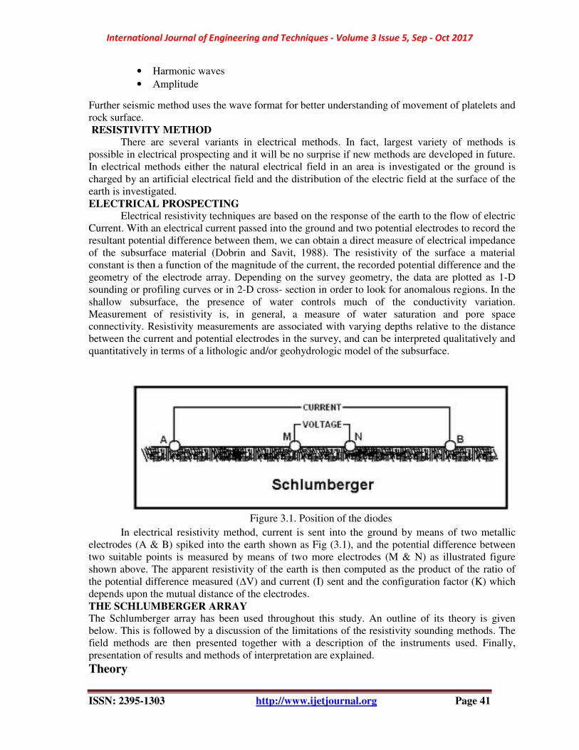
Figure 3.1. Position of the diodes

In electrical resistivity method, current is sent into the ground by means of two metallic

electrodes (A & B) spiked into the earth shown as Fig (3.1), and the potential difference between

two suitable points is measured by means of two more electrodes (M & N) as illustrated figure

shown above. The apparent resistivity of the earth is then computed as the product of the ratio of

the potential difference measured (∆V) and current (I) sent and the configuration factor (K) which

depends upon the mutual distance of the electrodes.

THE SCHLUMBERGER ARRAY

The Schlumberger array has been used throughout this study. An outline of its theory is given

below. This is followed by a discussion of the limitations of the resistivity sounding methods. The

field methods are then presented together with a description of the instruments used. Finally,

presentation of results and methods of interpretation are explained.

Theory



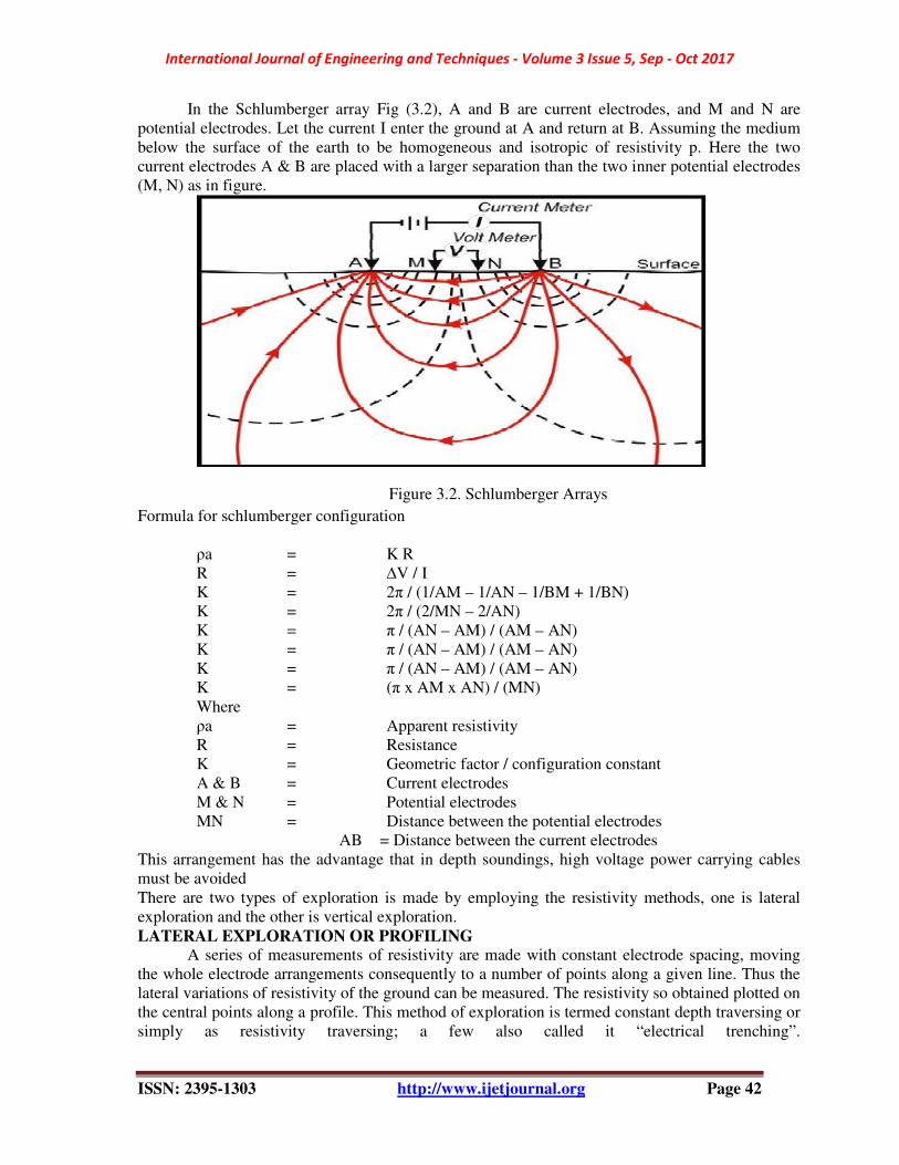
In the Schlumberger array Fig (3.2), A and B are current electrodes, and M and N are

potential electrodes. Let the current I enter the ground at A and return at B. Assuming the medium

below the surface of the earth to be homogeneous and isotropic of resistivity p. Here the two

current electrodes A & B are placed with a larger separation than the two inner potential electrodes

(M, N) as in figure.

Figure 3.2. Schlumberger Arrays

Formula for schlumberger configuration

ρa = K R

R = ∆V / I

K = 2π / (1/AM – 1/AN – 1/BM + 1/BN)

K = 2π / (2/MN – 2/AN)

K = π / (AN – AM) / (AM – AN)

K = π / (AN – AM) / (AM – AN)

K = π / (AN – AM) / (AM – AN)

K = (π x AM x AN) / (MN)

Where

ρa = Apparent resistivity

R = Resistance

K = Geometric factor / configuration constant

A & B = Current electrodes

M & N = Potential electrodes

MN = Distance between the potential electrodes

AB = Distance between the current electrodes

This arrangement has the advantage that in depth soundings, high voltage power carrying cables

must be avoided

There are two types of exploration is made by employing the resistivity methods, one is lateral

exploration and the other is vertical exploration.

LATERAL EXPLORATION OR PROFILING

A series of measurements of resistivity are made with constant electrode spacing, moving

the whole electrode arrangements consequently to a number of points along a given line. Thus the

lateral variations of resistivity of the ground can be measured. The resistivity so obtained plotted on

the central points along a profile. This method of exploration is termed constant depth traversing or

simply as resistivity traversing; a few also called it “electrical trenching”.



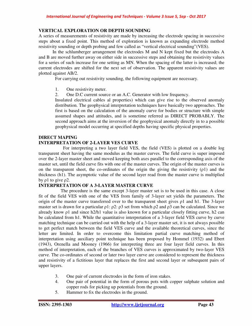
VERTICAL EXPLORATION OR DEPTH SOUNDING

A series of measurements of resistivity are made by increasing the electrode spacing in successive

steps about a fixed point. This method of exploration is known as expanding electrode method

resistivity sounding or depth probing and few called as “vertical electrical sounding”(VES).

In the schlumberger arrangement the electrodes M and N kept fixed but the electrodes A

and B are moved further away on either side in successive steps and obtaining the resistivity values

for a series of such increase for one setting as MN. When the spacing of the latter is increased; the

current electrodes are shifted for the next set of observation. The apparent resistivity values are

plotted against AB/2.

For carrying out resistivity sounding, the following equipment are necessary.

1. One resistivity meter.

2. One D.C current source or an A.C. Generator with low frequency.

Insulated electrical cables al properties) which can give rise to the observed anomaly

distribution. The geophysical interpretation techniques have basically two approaches. The

first is based on the calculation of the anomaly curve for bodies or structure with simple

assumed shapes and attitudes, and is sometime referred as DIRECT PROBABLY. The

second approach aims at the inversion of the geophysical anomaly directly in to a possible

geophysical model occurring at specified depths having specific physical properties.

DIRECT MAPING

INTERPRETATION OF 2-LAYER VES CURVE For interpreting a two layer field VES, the field (VES) is plotted on a double log

transparent sheet having the same modulus as the master curves. The field curve is super imposed

over the 2-layer master sheet and moved keeping both axes parallel to the corresponding axis of the

master set, until the field curve fits with one of the master curves. The origin of the master curves is

on the transparent sheet, the co-ordinates of the origin the giving the resistivity (ρ1) and the

thickness (h1). The asymptotic value of the second layer read from the master curve is multiplied

by ρ1 to give ρ2.

INTERPRETATION OF A 3-LAYER MASTER CURVE

The procedure is the same except 3-layer master set is to be used in this case. A close

fit of the field VES with one of the VES from family of 3-layer set yields the parameters. The

origin of the master curve transferred over to the transparent sheet gives ρ1 and h1. The 3-layer

master set is drawn for a particular ρ1: ρ2: ρ3 set from which ρ2 and ρ3 can be calculated. Since we

already know ρ1 and since h2/h1 value is also known for a particular closely fitting curve, h2 can

be calculated from h1. While the quantitative interpretation of a 3-layer field VES curve by curve

matching technique can be carried out with the help of a 3-layer master set, it is not always possible

to get perfect match between the field VES curve and the available theoretical curves, since the

letter are limited. In order to overcome this limitation partial curve matching method of

interpretation using auxiliary point technique has been proposed by Hommel (1932) and Ebert

(1943), Orenella and Mooney (1966) for interpreting three are four layer field curves. In this

method of interpretation, each of the branches of VES curves is approximated by two-layer VES

curve. The co-ordinates of second or later two layer curve are considered to represent the thickness

and resistivity of a fictitious layer that replaces the first and second layer or subsequent pairs of

upper layers.

3. One pair of current electrodes in the form of iron stakes.

4. One pair of potential in the form of porous pots with copper sulphate solution and

copper rods for picking up potentials from the ground.

5. Hammer to fix the electrodes in the ground.



INTERPRETATION OF FIELD VES CURVES

The final objective of conducting VES in field is to transform the field data in terms

of subsurface geology. Mainly there are two approaches. Qualitative and quantitative one of which

is used in interpreting the field VES.

QUALITATIVE METHODS OF INTERPRETING VES

Qualitative interpretation generally aims at locating areas where the geophysical field is

distributed and forming some ideas about the extent, shape, attitude, depth etc. of the subsurface

objects as judged from the shapes of anomalies either from visual observations or by using some

empirical values.

The qualitative analysis of the sounding data involves the following.

1.Study of apparent resistivity maps.

2.Study of apparent resistivity sections.

3.Study of first derivative maps.

4.Study of residual apparent resistivity sections which are analogous to residual gravity by

the removal of regional or background values.

QUANTITATIVE INTERPRETATION

This generally aims to determine a geophysical model (with a chosen shape and attitude,

depth and physical structure)

These fictitious or equivalent layer parameters are represented in graphical form called the

auxiliary charts which are available one of each type namely, H, Q, A and K.

REVIEW OF LITERATURE Nepal et al (2010) followed efficacy of electrical resistivity and induced polarization

method methods for revealing fluoride contaminated groundwater in granite terrain.

Resistivity sounding results supplemented by IP sounding data are useful for delineating the

fluoride contaminated aquifers in the granite terrain. The aquifers showing a correlation of

low resistivity ( 7.42 – 8.00 ohm m ) by low chargeability ( 1.5 -2.8 ms) are indicative of

high fluoride concentration in ground Water study area.

Owen et al ( 2005) studied multi -electrode resistivity survey for groundwater

exploration in the Harare greenstone Zimbabwe . The ability of multi – electrode resistivity

profiling to provide a detailed continuous 2 D map of the subsurface , identifying the

different lithologies , delineating contact zones and faults, and measuring the thickness of a

weathered regolith , makes this technique a very useful tool for groundwater investigations,

both for locating drilling sites and for obtaining an assessment of the general extent of the

depth of weathering and the location of fractured zones, which are the principal groundwater

reservoirs. John and Anthony (2010) studied 2 D electrical imaging and its application in

ground water exploration in part of river basin – zaria , Nigeria . The electrical imaging

method has in the past proved to be a powerful technique in the subsurface geology.

Abiola et al ( 2009) studied ground water potential and aquifer protective capacity of

overburden units in ado- ekiti , southwestern Nigeria . In this study, the groundwater potential

and protective capacity evaluation of rock units around ado- ekiti south western Nigeria was

undertaken 51 schlumberger vertical electrical soundings ( V E S) . The curve type varied

from simple three layers A, K and H types to the complex HQ , KH , HA , KQ , HK , HKH ,

HAA , KQH , KHK , and QHK types . The computer assisted sounding interpretation

revealed subsurface sequence composing topsoil with limited hydrologic significance,

weathered layer, partially weathered / fractured basement and fresh basement. The high

variability of the thickness of the top soil appeared responsible for observed overlapping

resistivity across the study area. The weathered layer constituted the sole aquifer unit in the



area; the yield being dependent on degree of clay content. The higher the clay content, the

lower the groundwater yield.

Lyndsay et al (2006) studied canal leakage potential using continuous resistivity

profiling techniques, western Nebraska and eastern Wyoming. Resistivity techniques were

successful in detecting changes in grain size along interstate and tristate canals. Both CC and

DC resistivity techniques were capable of mapping coarse – grained sediments. Canal

leakage can be more accurately simulated in ground water models. Improved understanding

of hydrogeology. Areas of maximum ground water- recharge.

Sabet (1975) studied vertical electrical soundings to locate ground water resources: a

feasibility study. This is because the resistivity of water – bearing sands depends mainly on

the salinity of the water, the degree of saturation, and the presence of clay and slits. The

resistivity of clean sands (not containing shale or silt) and gravel saturated with fresh water

ranges between 20 and several hundred ohmmeter. On the other hand, the resistivity of the

same and containing silt , clay or brackish water is much lower. It is thus established that

fresh ground water is unlikely produced from horizons of resistivity less than 10 ohm meter.

Gnanasundar and elango (1999) assessed the groundwater quality using geoelectrical

techniques .They have identified areas of sea intrusion , between 450m and 2200m , along

the coastal aquifer as well as sea water intrusion.

Senthilkumar et al ; (2001) studied geophysical studies to determine hydraulic

characteristics of alluvial aquifer .The hydraulic conductivity of the study area was found to

be range from 21 to 74 m/day . The transmissivity was found to be range from 390 to 1100

m^2/ day. This study shows the geoelectrical methods can be used not only for qualitative

measurements , but also for quantitative estimates of aquifer properties.

Mahmoud et al (2009) studied geoelectrical survey for groundwater exploration at

the asyuit governorate , nile valley , Egypt . A superficial geo electrical layer mainly covered

the ground surface of the area under investigation with relatively high electrical resistivity

values ( 105 – 40400 ohm –m ) and varied depth ( 0.43 – 35 m) . This wide ranges of the

electrical resistivity values are due to dry nature and percentage of gravel and sand.

Alabi et al (2010 ) studied determination of ground water potential in lagos state

university , ojo; uses dielectric methods( vertical sounding and horizontal profiling ) . It is

observed that VES is not so different from the horizontal profiling , because both the

methods gave depth , thickness and resistivity . So it cannot be said that one method is

better than the other .

Amadi et al (2011) studied evaluvation of ground water potential in pompo village ,

gidan kwano , menu using vertical electrical resistivity sounding . groundwater exploration

in the basement is based on weathered basement aquifer and fractured basement aquifer .

The contour plots revealed that then central portion of the study area has a potential for

groundwater development . Despite all the limitations of the verse technique , it has been to

be reliable for groundwater exploration in the basement complex terrain , particularly when

using the schlumberger configuration and combining it with adequate geological mapping

and using computer aided interpretation of the survey data.

Clark and Richard (2011) studied inexpensive geophysical instruments supporting

ground water exploration in developing nations . With the cost so reasonable ( less than 850

dollars ) this equipment should become common among those desiring to provide water in

developing countries . The instruments are small , light , robust , inexpensive and easy to

construct . With the free software available the interpretation of data is not difficult ,

although care is still needed.

Joseph olakunle coker (2012) vertical electrical sounding ( VES ) methods delineate

potential groundwater aquifers in akoo area , Ibadan , southernwestern Nigeria .

Groundwater potential aquifers producing zones have been delineated through investigation



conducted by electrical resistivity survey . Weathered and fractured horizons have been

identified in the study area underlying VES stations , and all of these constitutes the aquifer

zones. Good prospects therefore exist for groundwater development in the study area where

the depth to bedrock and high resistivity value have a lower potential aquifer .

Rosli saad et al ( 2012) groundwater deduction in alluvium using 2-D electrical

resistivity tomography ( ERT) . Groundwater will lower the resistivity value and silt also will

bring down the resistivity value lower than the groundwater effect.

Mohamed metwaley et al (2012) groundwater exploration using geoelectrical

resistivity technique at Al- quwy yia area central Saudi Arabia . Resistivity surveys were

carried out in Al Quwy’ yia area at the central part of Saudi Arabia to map the aquifer and

groundwater potentiality in promising area close to Riyadh . The results of 1D and 2D

resistivity data interpretation indicated the depth to basement at the southwestern part of the

study area as well as the contact boundary between the basement complex and sedimentary

rocks .

The static water table is found to be matching with the limestone rock as indicated

from the comparison between the individual VES and the two wells in the study area . The

thickness of the aquifer is increasing in the north eastern part where the possibility is of

groundwater potentiality is increasing .The results of 1D data set were confirmed by 2D

section interpretation . The difference between two data sets are observed only in the shallow

parts as the 1D inversion is collected in dense manner and constrained with the available

geological information . Collecting more data using deep VES and time domain

electromagnetic are recommended for more analysis of the aquifer in the eastern part of the

study area.

Yadav and shashi kant ( 2007) studied integrated resistivity surveys for delineation of

fractures of groundwater exploration in hard rock areas. The efficacy of combined gradient

profiling ( GP ) and geoelectrical sounding (G S) using schlumberger configuration is

presented here to map the weathered and fractured zones in hard rock areas . The present

study clearly indicates the exploration of ground water resources can be done with a proper

planning especially in the hard rock areas.

Meena ( 2011 ) studied exploration of ground water using electrical resistivity

method . The NIT Rourkela topography and its surroundings receive an average rainfall of

around 130 cm and thus there is a great need of recharge of ground water . But due to this

diversity in types of deposits or formations the quality of groundwater is not satisfactory .

Also because of urbanization and growth of industry , there always a risk of water pollution

inside the ground water basin . For this reason it becomes important to correctly investigate

the quality of the groundwater before making them for use . In prospect of the discharge

obtained from the surveyed point it is originate that the point is highly potential for utilization

of ground water .If all points will be collectively taken into consideration for exploitation

the water necessity of the campus and the halls together with academic areas can be meet

adequately. Ground water can also be exploited through large diameter water table dug wells

in the valley from the unconfined aquifers . On the other hand water from these wells has to

be treatd before making them for domestic and other uses.

Srivatsava et al ( 2012) studied the study and mapping of ground water prospect

using remote sensing . GIS and geoelectrical resistivity techniques – a case study of

Dhanbad district , Jharkhand , India . Geologically it is observed that the ground water is

mainly confined to secondary porosity i.e . fractured zone , fault , joint and weathered

column . It is observed from the field survey and also from various wells located in region

,the hard granite gneisses and meta basic dykes sometimes act as barriers for the ground

water flow in the region .



Selvam and Subramanian (2012) studied groundwater potential zones identification

using geoelectrical survey : A case study from medak district , Andrapradesh district , India

. The presnt work has shown that in the hard rock environment , vertical electrical sounding (

VE S) has proved to be very reliable for ground water studies and therefore this method can

be excellently used for shallow and deep underground water geophysical resistivity

investigation . The most part of the study area consist of good quality of ground water

because the study area is dominated by the H type curve . The top layer is the black cotton

soil and is followed by weathered zone, which is H by basement rock . The best layer which

act as the good aquifer of medak districts is the second layer which consists of the fracture /

weathered rock formations of the depth between 5m and 15m

Lateef ( 2012 ) studied geophysical investigation for groundwater using electrical

resistivity method – A case of annunciation grammer school , Ikere Lga , Ekiti state , South –

western Nigeria . Vertical electrical sounding technique of the electrical resistivity method

has proven to be successful and highly effective in the identification and delineation of

subsurface structures that are favourable for ground water accumulation in a crystalline

basement complex area . The electrical resistivity survey method used in this project entails

locating a favorable borehole at annunciation school , Ikere – Ekiti revealed five subsurface

geo electrical layers. These consist of topsoil , weathered layer and the fractured basement .

However the fractured basement is found in all the segments of the study area

Elasyed I.selim et al (2010) used two dimensional (2D) electrical resistivity imaging

at the western shore of old Luxor city , Egypt . The geophysical survey methods offer the

possibility of characterize and reconstruct the subsurface without destroying the minerals .

The interpretation 2 – D resistivity imaging shows that there are two layer arranged from the

top to bottom of the soil as solid layer consist of weathered clay. N. Kazakis et al (2016)

used ERT to determine the geometrical characteristics of saline aquifer . An abnormal

distribution of sea water intrusion was recorded by using the ERT (electrical resistivity

technique ) . The advantage of using ERT is that more data can be collected without a

limited hydrochemical samples.

METHODOLOGY There are several variants in electrical methods. In fact, largest variety of methods is

possible in electrical prospecting and it will be no surprise if new methods are developed in future.

In electrical methods either the natural electrical field in an area is investigated or the ground is

charged by an artificial electrical field and the distribution of the electric field at the surface of the

earth is investigated.

1.2 Electrical Resistivity Prospecting

Among the geophysical techniques, electrical resistivity methods enjoys the greatest

popularity and are widely used for both regional and detailed groundwater surveys because of

its better resolving power, less expenses as well as range of applicability.

The electrical resistivity methods has been used in this study in order to,

1. Delineate potential zones of ground water

2. Find out the thickness of saturated zones, depth to the basement topography

3. To determine the salt water-fresh water horizons with reference to space.

4.3. Apparent Resistivity

The ability to conduct current is an important physical property of rock forming

minerals and this property is made use of in electrical prospecting .Electrical resistivity

surveying is based on measuring of the resistivity ‘ρ’ of subsurface by passing a known

electric current into the ground and measuring the potential difference between two points.



The technique is based on the validity of Ohm’s law for linear conduction which is

represented as,

∆V

R = I

Where,

R = Resistivity in Ohm’s to the flow of current.

I = Current in Amperes

V= Potential difference in volts across the two end faces of a conductor

The resistance of the medium is directly proportional to its length ‘L’ and is inversely

proportional to its sectional area ‘A’, so that

R proportional to L/A

i.e., R = Ρl/A

or

ρ = R. A/L

While carrying out the survey in the field, either direct current or low frequency

alternating current introduced into the ground, through two current electrodes(A, B) and the

potential difference is measured between another pair of (potential) electrodes (M, N). By

considering the values of current, potential difference and the geometry of electrode

configuration it is possible to compute the resistivity of the material as

ρ = 2π x ∆V/ (1/AM-1/BM-1/AN+1/BN) x I

Where AM, BM, AN, and BN are the inter electrode distances.

The factor, 2π x ∆V

(1/AM-1/BM-1/AN+1/BN)

is referred to as the geometric constant K, of the

configuration used.

Hence,

ρ= K.∆V

I

The resistivity measured by the above method is said to be the true resistivity of the

medium only when the measurements are made over a homogeneous and isotropic medium.

As the earths subsurface generally is not so, the measured resistivity is not the true resistivity

and is said to be the ‘apparent resistivity’ (ρa).

4.4. Electrode configuration

In actual field measurement, a variety of electrode arrangements or configurations are

used, the difference being in the inter-electrode distance and geometry. The most commonly

employed configuration are the Wenner and Schlumberger arrangements.

4.4. a. Wenner Configuration

In the Wenner electrode array, all the four electrodes, equidistant with respect to each

other, are kept along a straight line, the outer two being the current electrodes .The inter

electrode distance is commonly denoted by the letter ‘a’. The relationship for apparent

resistivity ρa, for Wenner configuration is given by,

Pa = 2πaR

Where ‘a’ = distance between successive electrodes.

4.4. b Schlumberger Configuration The Schlumberger electrode configuration is also a symmetrical array like Wenner,

but differs in placing the two current electrodes with a much larger interval than that between

the potential (inner) electrodes. Only one set of electrodes either potential or current are



moved to expanded intervals at a time while conducting depth soundings unlike in Wenner

array where there are four electrodes are moved simultaneously. The current electrodes are

denoted by A and B, while the potential electrodes are denoted by M and N. The interval

between M and N is denoted by ‘b’ while the interval AB is denoted by’ a’. The apparent

resistivity is given by,

ρa = KR;

K = π AM . AN ;

MN

K= Configuration constant

R = Obtained resistance

There are several other electrode configurations which are modifications of Wenner

and Shlumberger arrangements, such as Lee partitioning, Carpenter tri-electrode

arrangement, Single arrangement and Dipole system of electrode arrangement.

4.5. Field Procedure

Resistivity methods are employed for both lateral and vertical exploration

1. Resistivity profiling for lateral exploration,

2. Resistivity sounding for vertical exploration.

4.6. Resistivity Profiling

Horizontal profiling is done to examine lateral variations in the subsurface in the area

of interest. A series of measurements of resistivity are carried out with constant electrode

spacing, moving the whole of the electrode arrangements consecutively to a number of points

along a given line. The apparent resistivities so obtained are plotted on the central points of

the array along a profile. This method is also termed ‘Constant depth traversing or Electrical

trenching’. Structures like dyke, faults, shear zones (apart from changes in rock types) etc,

which are generally associated with lateral variations, can be investigated by the profiling

method.

4.7. Vertical Electrode Soundings (V.E.S)

In resistivity sounding, the measurements are made at one location (keeping the centre

of the electrode system fixed) for various values of current electrode separations starting from

an initially small value to several hundred meters, depending on the depth of interest. This is

because, in general, larger the electrode separation, greater will be the depth of investigation.

The variation of the apparent resistivity with current electrode separation thus obtained would

give the variation in the electrical characteristics of the formation with depth. This method

(V.E.S) is most commonly applied for groundwater investigations and will be discussed in

detail in this project work.

Resistivity survey should be made paying due attention to possible disturbing

elements such as pipe lines, wire fences, rail tracks, etc. These methods cannot be used in the

vicinity of power plants, substations, high tension power lines and similar sources of

extraneous earth currents which would adversely affect the accuracy of the field

measurements.

4.8. Interpretation of Resistivity data

Interpretation of the electrical resistivity data in terms of the subsurface geology and

hydrology forms two most important phase in the exploration of groundwater. The aim of

interpretation of resistivity is to determine the thickness and resistivity of different horizons

present. Interpretation of V.E.S data is both quantitative and qualitative. The type of V.E.S

curve obtained indicates the qualitative nature of subsurface that may be expected in an area.



For example; a H type curve in a hard rock terrain may be interpreted as comprising of (1) a

dry top soil cover followed by (2) moist weathered rock/regolith, underlain by (3) the bed

rock. There are many ways to interpret the resistivity data starting from empirical method to

sophisticated techniques using fast computers. In this project work all the resistivity data are

interpreted with the help of Auxiliary Point Chart (APC) Method.

4.9. Auxiliary Point Chart Method

A much faster way of solving a V.E.S curve makes use of two layer theoretical curves

and the so called Auxiliary Point Charts (Bhattacharyya and Patra, 1968). Two Auxiliary

chats are needed H-type for A and H-typeV.E.S curves and Q-type for Q and K type curves.

This method can be used for solving three or more layered VES curves.

The first part of the curve (two layers) is matched with either the ascending or

descending two-layer theoretical curves, as the case may be and the origin of the type curve is

marked on the field curve sheet. The co-ordinates of the origin of the master curves as read

on the field curve will give the value of ρ1 and h1 (resistivity and thickness of the first layer).

The theoretical curve also gives the ratio of ρ2/ρ from which ρ2 can be calculated.

There are four types of three layer curves. They are H-type, A-type, K-type and Q-

type of curves. In the H-type the resistivity of the intermediate layer is layer(ρ2) is lower than

top layer (ρ1) and bottom layer(ρ3), i.e. ρ1>ρ2>ρ3. In A-type curve, the intermediate layer (

ρ2 ) is more resistive than first layer but less resistive than the third layer, i.e.ρ1<ρ2<ρ3. In

Q-type the resistivity of the intermediate layer is less than that of the top and bottom layer,

i.e. ρ1>ρ2>ρ3.

While interpreting a three layer field curve, the left hand part of the curve is

superposed on the suitable set of two layer master curve and the values of ρ1 and h1 are

obtained. The right hand part of the field curve is matched with the suitable two layer master

curve and the origin of this match gives the ratio ρ3/ρe,ρe is read from the graph and ρ3 is

calculated. Then the field curve is superposed on the proper set of Auxiliary Point Chart (i.e.,

A, K and Q) with the points (h1, ρ1) on the origin of the chart, and the ratio h2/h1 is read

from the chart, and h2 can be calculated.

Interpretation of four layer and multi layer curves involve the same procedure as described

above, but in this case the field curves has to broken up in to more than two parts depending

upon the number of layer encountered. All the field curves obtained from the study area were

interpreted using this Auxiliary Point Chart method.

RESISTIVITY INVESTIGATIONS IN THE STUDY AREA

4.1. Resistivity field work

Vertical electrical soundings were carried out in the field by using shlumberger configuration.

In all 11 soundings were carried out from Thiruporur to Mahabalipuramand analyzed. The

minimum and maximum values of AB/2 chosen for the surveys are 1 meters to 60 meters.

The field VES curves are discontinuous in nature, the discontinuity caused by the shifting of

potential electrodes during the soundings. For analysis of VES curves, a continuous curve is

required and this is obtained by smoothening of field curves. The smoothening was done by

shifting the curve segments parallel to AB/2 axis till all the segments are joined together. The

apparent resistivity data of VES locations have been plotted on log-log graph and matched

with the master curves for obtaining the layer parameters (resistivity and thickness). Results

of VES interpretation is given in the Table.4.1.



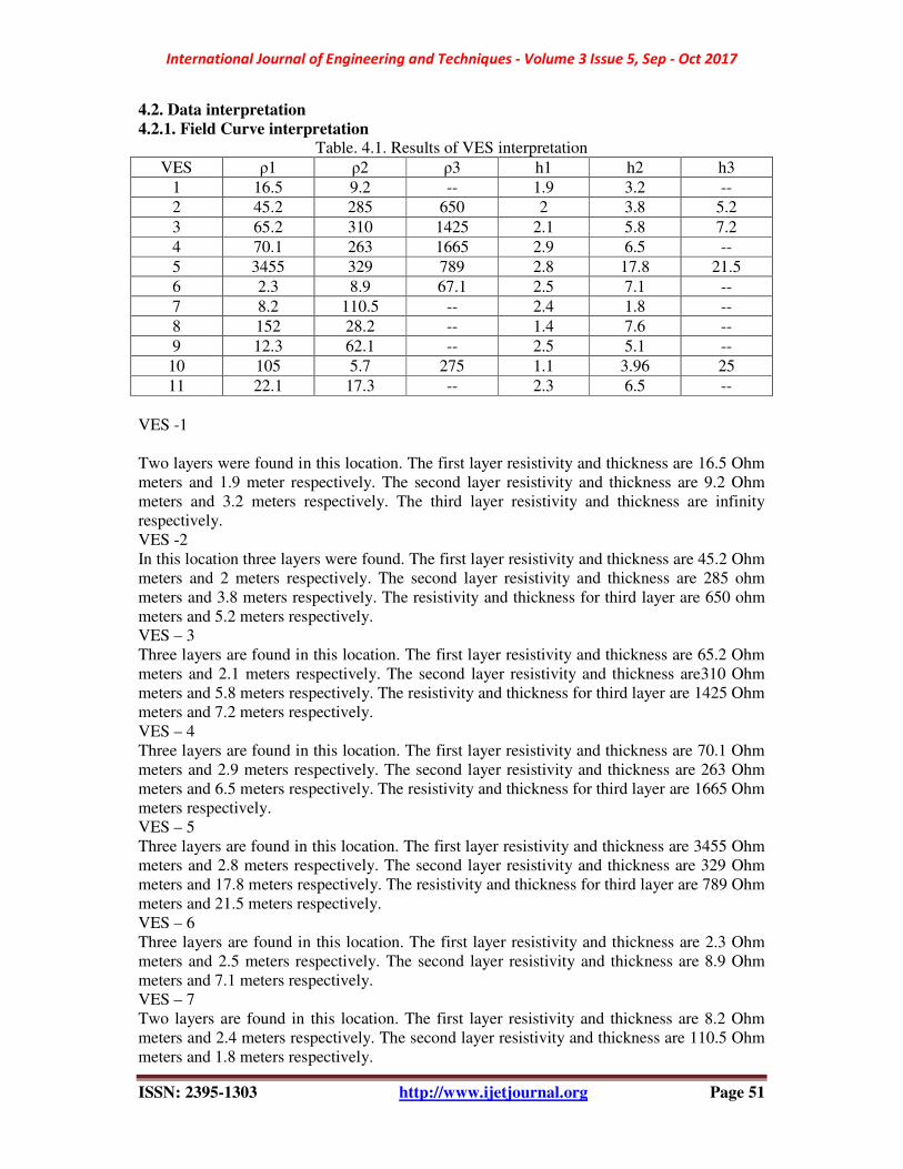
4.2. Data interpretation

4.2.1. Field Curve interpretation

Table. 4.1. Results of VES interpretation

VES ρ1 ρ2 ρ3 h1 h2 h3

1 16.5 9.2 -- 1.9 3.2 --

2 45.2 285 650 2 3.8 5.2

3 65.2 310 1425 2.1 5.8 7.2

4 70.1 263 1665 2.9 6.5 --

5 3455 329 789 2.8 17.8 21.5

6 2.3 8.9 67.1 2.5 7.1 --

7 8.2 110.5 -- 2.4 1.8 --

8 152 28.2 -- 1.4 7.6 --

9 12.3 62.1 -- 2.5 5.1 --

10 105 5.7 275 1.1 3.96 25

11 22.1 17.3 -- 2.3 6.5 --

VES -1

Two layers were found in this location. The first layer resistivity and thickness are 16.5 Ohm

meters and 1.9 meter respectively. The second layer resistivity and thickness are 9.2 Ohm

meters and 3.2 meters respectively. The third layer resistivity and thickness are infinity

respectively.

VES -2

In this location three layers were found. The first layer resistivity and thickness are 45.2 Ohm

meters and 2 meters respectively. The second layer resistivity and thickness are 285 ohm

meters and 3.8 meters respectively. The resistivity and thickness for third layer are 650 ohm

meters and 5.2 meters respectively.

VES – 3

Three layers are found in this location. The first layer resistivity and thickness are 65.2 Ohm

meters and 2.1 meters respectively. The second layer resistivity and thickness are310 Ohm

meters and 5.8 meters respectively. The resistivity and thickness for third layer are 1425 Ohm


VES – 4


meters and 2.9 meters respectively. The second layer resistivity and thickness are 263 Ohm


meters respectively.

VES – 5

Three layers are found in this location. The first layer resistivity and thickness are 3455 Ohm

meters and 2.8 meters respectively. The second layer resistivity and thickness are 329 Ohm



VES – 6


meters and 2.5 meters respectively. The second layer resistivity and thickness are 8.9 Ohm


VES – 7

Two layers are found in this location. The first layer resistivity and thickness are 8.2 Ohm





VES – 8

Two layers are found in this location. The first layer resistivity and thickness are 152 Ohm



VES – 9




VES – 10

Three layers are found in this location. The first layer resistivity and thickness are 105 Ohm



meters and 25 meters respectively.

VES – 11




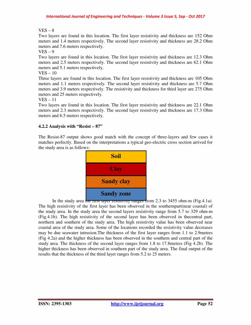
4.2.2 Analysis with “Resist – 87”

The Resist-87 output shows good match with the concept of three-layers and few cases it

matches perfectly. Based on the interpretations a typical geo-electric cross section arrived for

the study area is as follows:

In the study area the first layer resistivity ranges from 2.3 to 3455 ohm-m (Fig.4.1a).

The high resistivity of the first layer has been observed in the southernpart(near coastal) of

the study area. In the study area the second layers resistivity range from 5.7 to 329 ohm-m

(Fig.4.1b). The high resistivity of the second layer has been observed in thecentral part,

northern and southern of the study area. The high resistivity value has been observed near

coastal area of the study area. Some of the locations recorded the resistivity value decreases

may be due seawater intrusion.The thickness of the first layer ranges from 1.1 to 2.9metres

(Fig 4.2a) and the higher thickness has been observed in the southern and central part of the

study area. The thickness of the second layer ranges from 1.8 to 17.8metres (Fig 4.2b). The

higher thickness has been observed in southern part of the study area. The final output of the

results that the thickness of the third layer ranges from 5.2 to 25 meters.

Soil

Clay

Sandy clay

Sandy zone



ρ1 ρ2

Fig.4.1. Spatial distribution of resistivity layers one ρ1 and two

h1 h2

Fig.4.2. Spatial distribution of thickness of first layers (h1) and second(h2) RESULTS AND CONCLUTION

Geologically the study area comprises of charnokite rocks of Precambrian complex and

dolerites, which is classified as hard rocks as far as Hydrogeology is concerned. Out crops of

these rocks are noticed in a few places. Joints and fractures are present in these rocks, these

are very favorable for groundwater potential and recharge. Alluvium is found from the

surface to a depth 5m in many places. This also increases the groundwater potential.The

electrical resistivity investigations were carried out to understand the subsurface conditions

prevailing in the area. Data is analyzed using curve matching techniques. Interpretation of

resistivity data shows the presence of saline water in the east of the study area as indicated by

the low resistivity values. Interpretation of resistivity data also reveals that the top soil cover



ranges from 1.2 meters to 2.2 meters followed by weathered zone and bedrock with very high

resistivity.

The high resistivity of the first layer has been observed in the southern part(near

coastal) of the study area. The high resistivity of the second layer has been observed in the

central part, northern and southernof the study area. The high resistivity value has been

observed near the coastal area of the study area. Some of the locations the resistivity values

decrease may be due seawater intrusion. The higher thickness of the first layer has been

observed in the southern and central part of the study area. The higher thickness of the second

layer has been observed in southern part of the study area.In conclusion, it can be said that

the electrical resistivity studies have helped in understanding the subsurface hydrology and

the occurrence of saline and brackish water in the northern and center part of the study area

indicating that it is contaminated by the landward migration of saline water from the

backwater in the area.A detailed work in this area will help as in understanding the geology

of the area and to determine the ground water potential zones to manage and enhance the

ground water with the help of rain water harvesting structures in the fractured, weathered and altered rock layers.

References:

1. Abiola O, enikanselu P.A and oladapo M.I 2009 – ground water potential and aquifer

protective capacity of overburden units in ado – ekiti , southwestern Nigeria . International

journal of physical sciences Vol . 4 (3) , pp 120-132.

2. Alabi A.A bello R, A.S Ogungbel and oyerinde H.O 2010 – Determination of groundwater

potential in lagos state university , ojo ; using geoelectric methods ( vertical electrical

sounding and horizontal profiling ). Report and opinion 2(5) : 68-75

3. Amadi A.N Nwawulu C.D Unuevho C.I Okoye N.O Okunolola I.A , Egharevba N.A

,AkoT .A and alkali Y.B .2011-evaluvation of groundwater potential in pompo village ,

Gidan kwano , Minna using electrical resistivity sounding . British journal of Applied

sciences and technology 1(3) : 53-66.

4. Chris R.Daniel , Heraldo L. Giacheti , john A. Howie and Richard G. 1999 – Resistivity

piezocone (RCPTU) Data interpretation and potential applications . Pan – American

conference , brazil .

geophysical investigation from thiruporur to ... · geophysical investigation from thiruporur to...

Documents