geophysical mapping of buried river channels and other
TRANSCRIPT

GEOPHYSICAL MAPPING OF BURIED RIVER CHANNELS AND
OTHER SHALLOW STRUCTURES RECHARGING MAJOR AQUIFERS
IN THE LAKE NAKURU BASIN, KENYA RIFT: CASE STUDY FROM
KABATINI AQUIFER
By
bAARON WASWA KUTUKHULU
156/70439/2008
Dissertation submitted in partial fulfilment for the degree of Master of Science in
Geology (Applied Geophysics) in the University of Nairobi
-August 2010
University of NAIROBI Library
0378852 8

DECLARATION
This is my original work and has not been submitted for a degree in any other University.
Signed
Aaron Waswa Kutukhulu
This dissertation has been submitted for examination with my knowledge as University
supervisor
Signed C ^ O (J
Professor Justus O. Barongo
ii

AbstractThe project covered the geophysical mapping of buried river channels and other shallow
structures recharging major aquifers in the upper Nakuru basin o f Kenya rift and in particular the
Kabatini area. The project aimed at unveiling scientific knowledge of the subsurface geology
using resistivity and magnetic geophysical methods. It also aims at solving water shortages and
improvement o f livelihood of the people o f Nakuru and its neighbor hood through proper and
more precise geophysical ground water exploration methods. The ultimate goal of the report is to
provide guidance to policy makers in decision making especially for ground water extraction in
Kabatini aquifer. Geology and hydrogeology of the area have been discussed in the report. The
methods used in the research and the expected outputs have also been mentioned in the report.
These field methods include vertical electrical sounding, electrical resistivity tomography and
magnetic survey. Data processing was done using Earth imager software, RES2DINV, and Euler.
The findings of the research ascertain that Kabatini area has underground river channel that
flows in the north - south direction. The research also shows that the area has some shallow
structures which contain low resistivity materials in different locations. It has also been
ascertained that the thickness of kabatini aquifer is more than 150 m.
iii

AcknowledgementI wish to thank my almighty God for the care, knowledge and wisdom He granted me during this
research. He is a wonderful God.
I am greatly indebted to Professor Justus Barongo, who constantly followed this work, and for
his invaluable advice, encouragement, useful criticisms, and for sparing his time to read this
dissertation and suggesting useful comments, and above all his sense o f humour and
understanding. I also express my profound gratitude to the Chairman of the department of
geology and the entire teaching staff for their support during my masters program.
It is with pleasure and gratitude that I thank the University of Nairobi and in particular the Board
of post graduate studies to have given me the scholarship for two years. I also appreciate the
hospitality and effective services o f the staff without singling any, of the Department of Geology
at the University o f Nairobi. I am grateful to my fellow students and friends who in many ways
assisted me during the period o f study.
I wish to acknowledge my Parents for their encouragement and prayers. As ever, the major
inspiration and encouragement comes from my daughters Miriam, Grace, and Martha, who
cannot be thanked adequately. Their encouragement, understanding, and patience, even during
hard times, is appreciated.
My God bless whoever participated directly or indirectly to the success of this dissertation.
iv

CONTENTSTitle page....................................................................................................................................... i
Declaration....................................................................................................................................ii
Abstract......................................................................................................................................... iii
Acknowledgement........................................................................................................................ iv
Table o f contents.......................................................................................................................... v
List of figures............................................................................................................................... vii
List of Tables................................................................................................................................ x
CHAPTER ONE
1.0 Introduction............................................................................................................................ 1
1.1 Background............................................................................................................................ 1
1.2 Nakuru Basin.......................................................................................................................... 3
1.2.1 Location of Nakuru Basin..................................................................................................3
1.2.2 Climate................................................................................................................................ 3
1.2.3 Vegetation........................................................................................................................... 4
1.2.4Land use ............................................................................................................................... 4
1.2.5 Drainage.............................................................................................................................. 4
1.3 Kabatini aquifer....................................................................................................................6
1.3.1 Location..............................................................................................................................6
1.3.2Accessibility ...................................................................................................................... 6
1.3.3 Climate.................................................................................................................................6
1.3.4 Vegetation........................................................................................................................... 6
1.3.5Land use and Land resources..............................................................................................8
1.3.6Drainage and Physiography................................................................................................8
1.3.7 Geology and Structures...................................................................................................... 11
1.4 Statement o f the problem..................7.................................................................................. 13
1.5 Aim of the research and the objectives................................................................................ 13
1.6 Justification and significance o f the research...................................................................... 14

CHAPTER TWO
2.0 Literature review.....................................................................................................................15
2.1 Geology and structures........................................................................................................... 15
2.2 Geophysics...............................................................................................................................18
2.3 Hydrogeology.......................................................................................................................... 19
2.4 Groundwater flow system..................................................................................................... 20
CHAPTER THREE
3.0 Basic principles o f the methods used in research................................................................ 22
3.1 Introduction.............................................................................................................................22
3.2 Basic theory.............................................................................................................................23
3.2.1 Electrical properties of earth material............................................................................... 27
3.2.2 Geoelectrical sections..........................................................................................................30
3.3 Basic principles of magnetic survey................................................................................... 32
3.4 Physics o f proton precession magnetometer.......................................................................33
CHAPTER FOUR
4.0 Field data acquisition.............................................................................................................36
4.1 Introduction............................................................................................................................. 36
4.2 Field surveys...........................................................................................................................37
4.2.1 Instrumentation............................ 38
4.2.2 Vertical electrical sounding instrumentation................................................................... 38
4.2.2.1 Vertical electrical sounding data acquisition............................................................... 40
4.2.2.2 Schlumberger’s configuration.........................................................................................41
4.2.3 Electrical resistivity tomography instrumentation...........................................................42
4.2.3.1 Electrical resistivity tomography data acquisition.......................................................43
4.2.4 Magnetic survey instrumentation...................................................................................... 47
4.2.4.1 Magnetic survey data acquisition'*.................................................................................. 47
CHAPTER FIVE
5.0 Data processing.......................................................................................................................51
5.1 Introduction............................................................................................................................. 51
5.2 Electrical resistivity tomography data processing............................................................... 51
5.3 Vertical sounding data processing........................................................................................53
vi

5.4 Magnetic survey data processing.........................................................................................54
5.5 Results and geological interpretation.................................................................................. 55
5.5.1 Interpretation o f vertical electrical sounding results.......................................................58
5.5.1 Comparison of the resistivity values of the four VES profiles.................................... 795.6 Iso - resistivity Maps.......................................................................... .................................79
5.6.1 2D Vertical Iso - resistivity maps.....................................................................................80
5.6.1.1 Vertical section Iso - resistivity map o f profile A -B ....................................................80
5.6.1.2 2D Vertical section of profile C -D ...................................................................................81
5 .6 .1.3 2D Vertical section of profile E-F.....................................................................................82
5.6.1.4 2D Vertical section of profile G-H....................................................................................83
5.6.2 Horizontal Iso-resistivity Maps..........................................................................................84
5.6.3 Interpretation of electrical tomography and magnetic data........................................... 92
5.6.4 Total magnetic anomaly distribution in the study area.................................................100CHAPTER SIX
6.0 Summary and conclusion......................................................................................................102
6.1 Summary..................................................................................................................................102
6.2 Conclusion................................................................................................................................104
6.3 Recommendation.....................................................................................................................105
Reference...................................................................................................................................... 106
List of figures
Figure 1.1 Location map forNakuru basin............................................................................... 3
Figure 1.2 Physiography ofNakuru basin................................................................................. 5
Figure 1.3 Location map of Kabatini aquifer............................................................................7
Figure 1.3a Photograph showing land use ................................................................................ 8
Figure 1.4 General Physiography with Bahati hills in background....................................... 9
Figure 1.5 General Physiography with Menengai crater in background............................... 9
Figure 1.6 Vegetation of the project area.................................................................................. 9
Figure 1.7 Drainage ofNakuru basin.........................................................................................10
Figure 1.8 Physiographical map of the area around Kabatini aquifer.................................... 11
Figure 1.9 Geological and Structural map o f the Nakuru basin.............................................. 12
Figure 2.1 Geology and faults in rift system............................................................................. 17
Figure 2.2 Geological structures in Nakuru basin.................................................................... 20
V II

Figure 2.3 Piezometric map of Nakuru basin............................................................................21
Figure 3.1 Single current electrode in homogeneous ground ................................................ 26
Figure 3.2 Two current electrodes in homogeneous ground.................................................. 26
Figure3.3 Arrangement o f the four electrodes.........................................................................27
Figure3.4 Different patterns that may be used in geophysical survey................................... 27
Figure3.5 Resistivity of common rocks, minerals and chemicals..........................................29
Figure 3.6 Two dimensional sections thickness of layers in schlumberger’s array..............30
Figure 3.7 A two layer section in schlumberger’s configuration............................................ 30
Figure3. 8 Three layer sections in Schlumberger’s configuration.......................................... 31
Figure 3.9 The Earth’s magnetic field........................................................................................32
Figure 3.10 Major elements of earth’s magnetic field.............................................................33
Figure 3.11 The arrangement o f proton magnetometer............................................................35
Figure 4.1 Map for ERT and Magnetic survey profiles...........................................................37
Figure 4.2 Map for ERT, VES and Magnetic survey profiles................................................ 38
Figure 4.2a Map for VES stations..............................................................................................40
Figure 4.3 Schlumberger configuration array............................................................................41
Figure 4.4 ERT equipment...........................................................................................................43
Figure 4.5 Field layouts for ERT equipment.............................................................................43
Figure 4.6 Author setting up ERT equipment............................................................................44
Figure 4.7 Author fixing the ERT cable..................................................................................... 45
Figure 4.8 Author entering data in SYSCAL R1 PLUS SWITCH 72 .................................... 46
Figure 4.9 Author taking magnetic data using GEOMETRICS-856.......................................49
Figure 5.1 Stages involved in processing ERT da ta ................................................................. 53
Figure 5.2 Stages involved in processing VES da ta ................................................................. 53
Figure 5.3 Stages involved in processing magnetic data..........................................................54
Figure 5.4 Relationship between F values and grain size.........................................................55
Figure 5.5 F values for BH 8 in Kabatini aquifer......................................................................56
Figure 5.6 Resistivity values of layered earth for station 1W, 0 ............................................. 59
Figure 5.7 Resistivity values o f layered earth for station 0 ,0 ................................................. 60
Figure 5.8 Resistivity values o f layered earth for station IE, 0 .............................................. 61
Figure 5.9 Resistivity values o f layered earth for station 2E, 0 .............................................. 63
viii

Figure 5.10 Resistivity values of layered earth for station 1W, IS..........................................64
Figure 5.11 Resistivity values of layered earth for station 0, I S .............................................65
Figure 5.12 Resistivity values of layered earth for station IE, IS ........................................... 67
Figure 5.13 Resistivity values of layered earth for station 2E, IS ...........................................68
Figure 5.14 Resistivity values of layered earth for station 1W, 2S..........................................69
Figure 5.15 Resistivity values of layered earth for station 0,2S.............................................. 71
Figure 5.16 Resistivity values of layered earth for station 1E,2S............................................72
Figure 5.17 Resistivity values of layered earth for station 2E, IS ...........................................73
Figure 5.18 Resistivity values of layered earth for station 1W, 3S..........................................74
Figure 5.19 Resistivity values of layered earth for station 0,3S.............................................. 76
Figure 5.20 Resistivity values of layered earth for station IE, 3S.....................................77
Figure 5.21 Resistivity values of layered earth for station 2E, 3S...........................................78
Fig 5.21a: ID resistivity earth models for the four profiles in Kabatini aquifer....................79
Figure 5.22: Vertical section for profile A - B..........................................................................80
Figure 5.23: Vertical section for profile C - D......................................................................... 81
Figure 5.24: Vertical section for profile E - F...........................................................................82
Figure 5.25: Vertical section for profile G - H......................................................................... 83
Figure 5.26 Iso-map at 50 m depth for Kabatini........................................................................85
Figure 5.27 Iso-map at 75 m depth for K abatini.......................................................................86
Figure 5.28 Iso-map at 100 m depth for Kabatini......................................................................87
Figure 5.29 Iso-map at 125 m depth for K abatini.....................................................................88
Figure 5.30 Iso-map at 150 m depth for K abatini.....................................................................89
Figure 5.31 Overlay o f Iso-maps................................................................................................ 90
Figure 5.32 Overlay o f Iso-map with 3D model........................................................................91
Figure 5.33 Pseudo-section o f profile A- B ............................................................................... 93
Figure 5.34 Electrical tomography image o f A-B......................................................................93
Figure 5.35 Magnetic anomaly showing buried river along A-B ...........................................94
Figure 5.36 Comparison of ERT, VES and borehole logs........................................................95
Figure 5.37 Electrical tomography image of profile C -D .........................................................96
Figure 5.38 Depth to magnetic source along profile C-D.........................................................97
Figure 5.39 Electrical tomography images along profile E-F.................................................. 97

Figure 5.40 Total magnetic field anomalies along profile E -F ...............................................98
Figure 5.41 Electrical tomography images along profile G-H................................................99
Figure 5.42 Total magnetic field anomaly along profile G -H ................................................100
Fig 6.1 Pseudo-sections showing buried river channel.............................................................102
Figure 6.2: River Ngosur traversing the four profiles............................................................... 103
Fig 6.3: The distribution of the total magnetic anomaly in Kabatini well field...................... 104
Tables
Table 2.1 Main stages o f rift development................................................................................ 16
Table 5.1 Borehole logs compared with VES log.................................................................... 57
Table 5.2 Layer thickness and resistivity for station 1 W,0........................................................59
Table 5.3 Layer thickness and resistivity for station 0,0............................................................60
Table 5.4 Layer thickness and resistivity for station 1E,0.........................................................62
Table 5.5 Layer thickness and resistivity for station 2E,0........................................................ 63
Table 5.6 Layer thickness and resistivity for station 1 W,1 S......................................................64
Table 5.7 Layer thickness and resistivity for station 0,1S.........................................................66
Table 5.8 Layer thickness and resistivity for station IE ,IS .......................................................67
Table 5.9 Layer thickness and resistivity for station 2E,1S...................................................... 68
Table 5.10 Layer thickness and resistivity for station 1 W,2S.................................................. 70
Table 5.11 Layer thickness and resistivity for station 0 ,2S ......................................................71
Table 5.12 Layer thickness and resistivity for station 1E,2S....................................................72
Table 5.13 Layer thickness and resistivity for station 2E,2S................................................... 73
Table 5.14 Layer thickness and resistivity for station 1 W,3S.................................................. 75
Table 5.15 Layer thickness and resistivity for station 0 ,3S ......................................................76
Table 5.16 Layer thickness and resistivity for station 1E,3S....................................................77
Table 5.17 Layer thickness and resistivity for station 2E,3S................................................... 78
x

CHAPTER ONE
1.0 Introduction
1.1 BackgroundBuried river channels are increasing becoming the target for groundwater exploration due to
the unreliability o f surface river channels that have been affected by climate changes. Areas
located in urban centers like Nakuru town have high population that dictates the higher
demand of water. Nakuru is located in an environmentally sensitive area, sandwiched
between Mau escarpment to the south west and the Menengai crater and its associated
volcanic landscapes to the north. To the north-east o f the town is the Bahati escarpment
which forms the western fringe o f the Aberdares escarpment. Lake Nakuru is the lowest point
in the region, at only 1,758 meters above sea level, and all rivers in the region drain into it.
Statistics suggest the population o f Nakuru has increased and its municipality expanded
tremendously. Large population increase implies a much increased demand for urban services
such as water. Increased population has further strained the existing water supply from the
available sources. The major economic sectors in Nakuru’s urban economy are commerce,
industry, tourism, agriculture and tertiary services. The commercial sector in Nakuru
contributes about 19 per cent to the economy o f the town. In the recent past, the water supply
in Nakuru has been characterized by chronic shortages affecting mainly residential and
industrial functions. The town has been getting its water from both surface and underground
water sources. Current climate changes have made surface water to be unreliable. Surface
water in Nakuru basin includes; River Njoro, Larmudiac, Makalia and Enderit (see fig 1.2)
which drain from Mau escarpment towards Lake Nakuru. Stream channels give a connotation
of ground water flow. The Ngosur River and several minor streams flow from the Bahati
forest towards the lake Nakuru, although none of them reaches the lake. The streams that
originate from Menengai disappear to become subsurface in the upper slopes o f the crater.
McCall, 1967 postulated that Ngosur River is controlled by the slope o f piedmont -plain
bounding the very straight north - west trending Bahati escarpment while other scientist who
have worked in this area suggest that buried rivers area controlled by the fault system .This
phenomenon o f conflicting information regarding disappearance o f rivers in Menengai and
Bahati plains called for integrated geophysical methods to determine the existence o f the
river channels in Kabatini area.
1

Geoelectrical resistivity techniques are popular and successful geophysical exploration for
study groundwater conditions in areas with complex geology. The resistivity o f material
depends on many factors such as groundwater, salinity, saturation, aquifer lithology and
porosity. For example, the resistivity o f an aquifer is related to Electrical Conductivity (EC)
of its water. When the groundwater EC is high, the resistivity o f the aquifer could reach the
same range as a clayey medium and the resistivity parameter is no longer useful to determine
the aquifer (Vouillamoz et al., 2002). However, this method has been carried out successfully
for exploration o f groundwater. This technique is widely used to determine depth and nature
o f an alluvium, boundaries and location o f an aquifer. The resistivity method has been used to
solve more problems o f groundwater in the alluvium, karstic and volcanic aquifers as an
inexpensive and useful method. Some uses o f this method in groundwater are: determination
of depth, thickness and boundary o f an aquifer (Zohdy, 1969; and Young et al. 1998),
determination o f interface saline water and fresh water (El-Waheidi, 1992; Yechieli, 2000;
and Choudhury et al., 2001), porosity o f aquifer (Jackson et al., 1978), and water content in
aquifer (Kesselsct al., 1985), hydraulic conductivity o f aquifer (Yadav and Abolfazli, 1998;
Troisi et al. 2000), transmissivity o f aquifer (Kosinski and Kelly, 1981), specific yield o f
aquifer (Frohlich and Kelly, 1987), contamination o f groundwater (Kelly, 1976; and Kaya,
2001). Contamination usually reduces the electrical resistivity o f pore water due to increase
o f the ion concentration (Frohlich and Urish, 2002). However, when resistivity methods are
used, limitation can be expected if ground inhomogeneties and anisotropy are present
(Matias, 2002). Investigations o f the subsurface water channels and other structures using
integrated geophysics remain the reliable solution to water shortages in Nakuru area.
2

1.2 Nakuru Basin
1.2.1 LocationNakuru basin is located in central part of the Kenya rift valley which forms part of the great
rift that passes through Ethiopia, Tanzania, Malawi and then to Uganda. The basin is bounded
by longitudes 32021’20” on the east 36° 10’ on the west and latitudes 0°13’15” on the north,
0°2830\ The Nairobi - Eldoret and Nairobi Kisumu roads pass through the basin.
1.2.2 Climate
Nakuru basin is generally hot and dry, with two rainy seasons; the long and the short rains.
The long rains start at the end of March and continue to the end of May, and the short rains
start at the end of October and continue to the end of December. The average rainfall varies
from 500 to 1300 mm with high altitude areas receiving more rain. The area is classified as
semi-humid to semi-arid. The mean average maximum temperature is 25°C and the average
minimum temperature is 12.3°C. The coldest months being July to August, while October
and March are the hottest as observed in Agro-climatic Zone Map of Kenya of 1980.
3

1.2.3 Vegetation
The forested areas o f the catchment basin consist o f the eastern Mau, northern Eburru, and
Bahati forests. The eastern Mau forest forms part o f a national watershed (the Mau
complex), being the largest o f these forest blocks. The vegetation surrounding the lake
consists o f a narrow belt o f fringing forest dominated by Acacia xanthophloes , scrub
communities on steep cliff encircling the southern part o f the lake (in some places
dominated by tall euphorbia, Euphorbis ingens)
1.2.4 Land use
About two-thirds o f the lake's drainage basin is used for agricultural purposes, mainly as
rangelands. Forest areas are found only along watershed ridges o f Mau Escarpment to the
west o f the lake. An extensive industrial area is rapidly growing around Nakuru City.
Grasslands with scattered shrubs used for cattle grazing.
Crop farming in the project area is mainly for subsistence purposes. The main food crops
grown include maize, beans, pigeon peas, cowpeas, sorghum and cassava. Land use activities
are very limited and vary in the project area these being governed by factors such as climate
(rainfall and temperature), soil conditions, altitude, and limited use o f farm inputs such as
pesticides and fertilizers. Most o f the remaining land in the area is used for large scale
commercial ranches (beef and dairy cattle). Dairy and beef cattle populations have increased
steadily over the years due to increased local demand from Nakuru town. Other livestock
reared in the district include sheep, goats, rabbits, pigs and bees.
1.2.5 Drainage
Nakuru basin lies within the Rift valley floor on the general nprthem slope o f the central
dome. Lake Nakuru is a basin o f internal drainage which is separated from lake Elementaita
by a low topographical devide. Lake Nakuru lies in a graben between Isirkon 2097m to the
east and Mau escarpment to the west, (Kuria, 1999). The Menengai crater (2280 meters
above sea level) on the northern part o f the basin and to the south lies the high ground o f Mau
and Eburr forest. Lake Nakuru is alkaline and saline a result o f evaporation and is recharged
by rainfall, surface runoff and groundwater. Drainage o f the basin is characterized by poor
surface runoff caused by existence o f highly porous and unsorted pumice rocks. River Njoro,
barmudiac, Makalia and Enderit (see fig. 1.2) drain from Mau escarpment towards Lake
4
Nakuru. The Ngosur river and several minor streams flow from the Bahati forest towards the
lake Nakuru, although non of them reaches the lake. The streams that originate from
Menengai disappear to become subsurface in the upper slopes of the crater. The drainage in
Nakuru basin is controlled by the faults. This is noted by sudden changes in the direction of
the water courses which respond to the general orientation of the Rift valley faulting.
PHYSIOGRAPHIC MAP OF NAKURU AREAE
0 2.5 5 10 15 20
Legend
----Ki lorn eters
© Towns Roads
Drainage Lakes
— ^ Rail_Forests
Figure 1.2: The Physiography of the Nakuru basin and its drainage system
5

1.3 Kabatini Aquifer
1.3.1 LocationThe study area lies in Nakuru district o f rift valley province in the Republic o f Kenya. It is
covered by Nakuru topographical map sheet 119/3 o f scale 1:50,000. Kabatini aquifer can be
located by coordinates S 0°15’36.6’/E 36°8’00.0” on the sheet 119/3 o f Nakuru. It is located
on the north eastern part o f Nakuru town. Nakuru town can be accessed by a tarmac road and
a railway line which forms part Trans Africa railway and road network from Nairobi. Nakuru
. Solai tarmac road passes on the western part o f the project area. A good earth road connects
to Nakuru - Solai road to the project area
1.3.2 AccessibilityKabatini aquifer is Nakuru town which is found in the central part o f the Kenyan rift. The
aquifer can be accessed from Nairobi through Solai road which connect Nairobi - Nakuru
road in Nakuru town. It occurs on the north eastern part o f Nakuru town (see fig 1.3).
1.3.3 ClimateKabatini area is generally hot and dry, with two rainy seasons; the long and short rains.
The long rains start at the end o f March and continue to the end o f May, and the short rains
start at the end o f October and continue to the end o f December. The average rainfall in the
project area varies from 700 to 981 mm. The project area is classified as semi-humid to semi-
arid. The mean average maximum temperature is 25°C and the average minimum
temperature is 12.3°C. The coldest months being July to August, while October and March
are the hottest as observed in Agro-climatic Zone Map o f Kenya (1980).
1.3.4 Vegetation
The vegetation found in Kabatini well field consists mainly of indigenous shrubs and grass
and exotic trees. The trees planted include Eucalyptus, Pinus patula, Grevillea robusta and
kei-apples (see fig. 1.3a and 1.5). Farmers also find the trees useful as windbreaks, for fencing
i and, in the long run, for fuel-wood or timber. There have been other motivators for farmers to
plant trees. The type o f vegetation cover is predominantly o f the exotic family since most of
the indigenous trees have been destroyed.
6

> AKl R l TOWN
Suda
Ethiopia
CongoMenengai forest
Lake Nakuru
Mau forest
S*M'30"S
0‘15(rJ|
D’ISW S
5' 6C sl
S’lS'WS
3S*S'0 36‘7':’E^y7j3* £ 36'6';-|
TO W A H l'K l 'R l
Bahati forest
Kabatim aquifer
Eburr forest
9’3C'E14 -30 S
OM7'0"t
.*g *n d
N ak„r-. • Nairobi roac __________> JL_1 1 Nakur^ tow r
k a o a tr i rcac
f#
j = t = n “
KABATTMAQITFTRM S re 1 Petrol station
♦ Primary Schoolif Chu-ch /
1E'(7S
.•tE'SO'S
16-ty s
:*I<5'30"S
TO N AIROBI
3‘ 17'30‘S •3 SIC 33SC
I7'<7S
:• 17'30'S
vy-iZ'E...Figure 1.3: location map of Kabatinfaquifer north - eastern part of Nakuru town.
7

1.3.5 Land useCrop farming in the project area is mainly for subsistence purposes. The main food crops
grown include maize, beans, pigeon peas and potatoes. Land use activities are very limited
and vary in the project area these being governed by factors such as climate (rainfall and
temperature), soil conditions, altitude, and limited use of farm inputs such as pesticides and
fertilizers. Most of the remaining land in the area is used for large scale commercial ranches
(beef and dairy cattle). Dairy and beef cattle populations have increased steadily over the
years due to increased local demand from Nakuru town. Other livestock reared in the district
include sheep, goats, rabbits, pigs and bees.
Figurel.3a: The photograph showing the land use in Kabatini area
1.3.6 Drainage and Physiography
Kabatini area has flat volcanic plains at an altitude of 2180 mt stretching on the western part
of the area running from Menengai creator towards Nakuru town (see fig 1.5). The similar
Physiography is also observed on the northern part of Kabatini aquifer stretching from Bahati
forest towards the Lake Nakuru (see fig. 1. 2 and 1.7), and a more gently sloppy country
formed by the volcanic rocks system varying from 1837 m to 2040 m on the southern part of
the project area. Generally Kabatini area is characterized by rolling terrain, with a notable
Menengai crater on the north western part (see fig 1.8). The terrain can be described as
generally flat to rolling; the highlands being the Menengai crater and Bahati
escarpment.There are two rivers in the northern part of Kabatini aquifer. These rivers are
8
river Ngosur and Menengai River. Menengai River flows towards the Menengai crater where
it disappears underground. Ngosur River flows in the south west direction and disappears
underground in Bahati plains.
Figure 1.4: The photograph of general Physiography of Kabatini area, see Bahati hills in the 'background. The photograph is taken facing in the Northern direction.
Figurel.5 The photograph shows the general Physiography of the project area, see Menengai crater at the background. The photograph was taken facing north western direction.
Figure 1.6 Vegetation (Grevillea robusta trees) in project area, the photograph was taken facing towards the south of the project area
9
f L X X X
LegendTowns
20i Kilometers
Roads
Drainage Lakes
Rail Forests
Figure 1.7 Drainage map ofNakuru basin.
10

}3'
'39
H
Legend
/ I ln««KjbJtn X|jii*r
■■■■■ MMMgJI WAt — Kivr
Figure 1.8 Physiographical map of the area surrounding Kabatini aquifer in Nakuru basin. The contours are seen to decrease towards the Lake Nakuru.
1.3.7 Geological setting of Kabatini aquifer
Kabatini has complex geological structures which have been subjected to several tectonic
processes leading to the formation of varying structural features. To northern side occurs
Menengai crater while to Bahati uplands occurs on the eastern part. The area is mainly
occupied by volcanic rocks which^consist of Vitric pumice tuff, ashes, agglomerates and
trachytes. The lake beds on the southern part of the area are composed mainly of volcanic
material and subsequently deposited pyroclastics. The sediments are composed of sand,
pebbles as well as gravels made up of rounded pumice, (MacCall, 1967).
11

GEOLOGICAL MAP OF THE AREA SHOWING FAULTS. MODIFIED FROM McCALL 1967.
4> -
4) ■
r
Legend
| Superficial deposits , Vitric pumice tuff
Olivine basalts Gravel Lakes
— — Roads
-t— t- Rail------ Drainage--------Faults
■ Towns
14 21 26
Figure 1.9: Geological and structural map of Nakuru basin
12

1.4 Statement of the problem
In the recent past, the water supply in Nakuru municipality, located within the Nakuru basin,
has been characterized by chronic shortages affecting mainly residential and industrial
functions. The municipality gets its water from both surface and underground water sources,
and it has about six major water reservoirs, Kabatini aquifer being one o f them. Kabatini
water wells have been experiencing draw downs in water levels in the recent past,
particularly during the dry season of the year. Kabatini area which is located in the
northeastern part o f Nakuru municipality is characterized by complex geology which has
affected the ground water system. River Ngosur found to the north disappears in the ground
in the northern part o f Kabatini in Bahati plains. It has never been proved that the river cannel
passes underground to recharge Kabatini aquifer. The main problem to be investigated in this
study is to determine if the aquifers in the Nakuru basin are recharged by river channels and
other shallow structures. In particular, it is to be proved if Ngosur River which disappears
underground in the north is actually the underground channel recharging the Kabatini aquifer.
The geological condition in the Kabatini area is complex and intricately related to the nature
of the groundwater regime, a fact that could be attributed to the difficulty to fully assess the
aquifer with the conventional hydrogeological methods alone. The entire area is covered by
volcano-sedimentary materials, intercalated lava flows. The exact distribution and depth o f
the lava has not been mapped.
l.S. Aim of the research and its objective
The aim o f this research is to map the buried river channels and other structures that sustain
constant recharge o f the main aquifers in the Nakuru basin using geophysics.
The objectives o f this research are;
1. To delineate the geometry o f any river channel(s) and other structures contributing to
the recharge o f the aquifers in Nakuru basin with the main focus on Kabatini.
2. To determine the depths o f the Kabatini aquifer and relate it to the number of
channels/structures recharging it.
13

1.6 Justification and significance of the research
Groundwater becomes the readily available option for exploitation in areas where surface
water shortages exist like the Nakuru basin. However, the over-exploitation o f this resource
has moved groundwater research to the forefront o f the geosciences in trying to answer the
questions o f groundwater recharge and discharge in aquifers. These questions become
increasingly relevant as we continue to test the limits o f groundwater resource sustainability
in areas o f complex geology like Kabatini area. Whereas other researchers have worked in the
area, none o f them has addressed the existence or non - existence o f the buried river channels
and other shallow underground structures that may be controlling groundwater flow systems.
The structures such as faults may form channels through which water flow and recharge the
aquifer. Geophysical methods are used to obtain accurate information about subsurface
structures like faults and buried river channels. The marginal rift faulting and the system of grid
faulting on the Rift floor have a substantial effect on the groundwater flow systems of the area. In
general faults are considered to have effects on groundwater flow. They may facilitate flow by
providing channels of high permeability, or they may prove to be barriers to flow by offsetting zones
of relatively high permeability. The methods used have proved to be efficient tools in groundwater
exploration. Not only have they been used in the direct detection of the presence of water but also in
the estimation of aquifer size, properties and mapping of buried valleys and rivers even in areas of
complex geology for direct drilling . The cost of drilling large-scale water-supply boreholes like in the
Kabatini area almost demands that the risk of drilling a poorly yielding borehole should be lessened
through the proper use of geophysics. The results in this research will be used to identify potential
drilling locations, decreasing the risk of drilling in unproductive areas that may waste the resources.
This complex nature o f the geology and the groundwater system in the upper Nakuru basin
makes a detailed and a systematic geophysical study, the appropriate alternative, as the
conventional hydrological approach so far has proved its inability to exhaustively deal with
the problem alone. Geophysical mapping in the area consists o f Electrical Resistivity
Imaging, Vertical Electrical Sounding and Proton Precession Magnetic Survey. These
methods are bound to reveal aspects that were not known in the project area.
Geophysical mapping o f buried rivers and other underground structures is one o f the tools
that will readily present conceptualized real-life situations and therefore provide quick
^swers to some o f the questions that policymakers, researchers, environmentalists, investors
ari(! other relevant authorities require before they make sound decisions within Nakuru and
Gsewhere in the world.
14

CHAPTER TWO
2.0 Literature Review
2.1 Geology and structures
Review of the previous geological and structural work was undertaken in order to understand
the origin o f Kabatini aquifer. The terrain under study is part o f a section o f the central Kenya
Rift Valley. The rift Valley is a Cainozoic intercontinental rift system separating the Somalia
sub - plate from the rest o f Africa (Smith and Mosley, 1993). The Rift valley system has a
north - south geographic trend delineated by faults with individual faults oriented at diverse
angles (Onywere, 1997). Step scarps mark flanks along fault lines, while the intervening
smaller faults are places marked by low, narrow hoist graben structures (Baker et al., 1972).
Part of the Rift valley in the study area is bordered on the eastern shoulder by an abrupt
topographic break, which is a surface trace o f the rift bounding Sattima fault. Mau
escarpment forms the boundary o f the basin on the western shoulder. The Kabatini aquifer
lies on the north eastern part o f the Nakuru basin within the Kenya rift Valley. The geology
of the area consists o f volcanic rocks which include basalts, phonolites, tuffs, and trachytes.
Rocks and structures within the rift valley where the project area is located have been
generated during the past 4 million years, (Clarke et al 1990). They are associated with the
full graben and inner trough stages o f the development o f the rift valley. The Rift margins
expose an older sequence o f trachytic, often ignimbritic, pyroclastics (the Mau and Kinangop
Tuff formations to the west and east respectively), and a younger thick sequence o f trachytic
flood lavas. Subsequent faulting produced the stepped escarpment which has an effect on the
drainage pattern and groundwater flow. Lake sediments form a large part o f the floor o f the
rift and are exposed in gullies, road sections and small quarries. Sand and pebble beds
dominate exposures o f lake sediments around the northern side o f the Olkaria Volcanic
Complex. Deposition in a high energyv possibly fluvial, environment is indicated by well-
tedded sand dominated sequences which show large-scale cross-bedding and channel
development.
15

Table 2.1 Main stages o f Kenya rift valley development, (Clarke et al 1990)
' s t a g e PRE-RIFT
DEPRESSION
HALF GRABEN FULL
GRABEN
INNER TROUGH
a g e 25-12 Ma Bp 12-4Ma 4-1.7Ma 1.7-OMa
t e c t o n ic Broad shallow Faulting in western Commencement Deepening o f axial
STYLE depressions part o f Turkana, of faulting on zone o f rift.
(warping) in the extending S-wards Eastern side of Extensional
Turkana region by 7 Ma rift. Grid
faulting.
tectonics in narrow
zones.
VOLCANISM Alkali Basalts Alkali basalts and Basalt/Trachyte Eruption o f flood
and basanites flood phonolites volcanism in Trachytes followed
erupted over e.g. Uasin-gishu central sector by grid
wide areas in and Yatta plateau, characterized faulting(<0.8 Ma).
the north. then transitional by very large Building o f a chain
Carbonatite- basalts and pyroclastics o f dominantly
/nephelinite Basalts/Trachyte eruptions. Trachytic caldera
volcanism in shield volcanoes Basalts less but volcanoes with
west Kenya and having marked Trachytes very alkali-rhyolite
the southern
rift, especially
on the south
and west flanks
o f the Kenya
Dome.
Daly gaps. widespread in
south and
extending east
over Nairobi
area mainly.
prominent in the
central sector.
SUMMARY PHONOLITE. TRACHYTE TRACHYTE and
BASALT and BASALT and often as large as BASALT in north.
NEPHELINITE TRACHYTE. large ash flows TRACHYTE,
RHOYOLITE and
minor BASALT in
south.
16

Bahati area is composed of well-rounded gravel and pebble-sized pumice and other
pyroclastic material which form the aquifer in that area. Many of the gullies that have
dissected parts of the rift floor have smooth floors as a result of the deposition of alluvial
sediments. Renewed down cutting in gullies on River Njoro in Nakuru has revealed that these
alluvial deposits are dominated by sand and gravel in the Basin.
36°!' 36°21'20"
0 ° m 5 '
i f A* AS
LECEMD?6° r
IU 0 10 20 Kilom eter*36°21'20"
*r*te;i» . Mactvl*.pf-i<r»c4fr&a»4tBasic ro ot M an Lno:«nj :il foofcR'.M .1icnsM'i n rrr»k
✓ V / faultCortous •.*A P*9L#1 IIS* 11
roadsYS/ *•♦»«
Figure 2.1: Geology and faults in the rift from Clarke, et al 1990.
17

2.2 Geophysics
There have been some geophysical studies in the past in the area on geothermal prospects.
These include regional gravity, aeromagnetic and resistivity soundings. Airborne Magnetic
survey data can provide vital information about regional structural features such as faults,
intrusions and basement rocks (that can be associated with an aquifer). The distribution of
magnetic properties in rocks can also give rise to a complex magnetic anomaly pattern or
signature which may be associated with a particular assemblage o f rocks. This pattern may
differ from the pattern over an adjacent rock type o f different lithology in amplitude level, in
number o f anomalies and in shape o f the anomalies. Criteria o f this sort allow many hidden
boundaries to be mapped out between often only limited areas o f exposure suitable for
conventional field mapping. Magnetic data covering the study area come from part o f the
African Database, Pastor, (2001). Barritt, 1993, contains the original source o f African
Magnetic Mapping Project (AMMP) results. The database is a compilation o f regional
magnetic anomalies o f several African countries that have been re-processed (upward
continued to 1000m) and merged together. The magnetic field intensity o f the study area is
34000 nT, at an inclination o f approximately -5° and a declination o f - l ° . The first presents
the gross magnetic intensity differences caused by different rock types like the mafic rocks
like the basalt outcrops and the felsic counterparts like the trachytes, rhyolites and
pyroclastics.
Measurement o f the electrical resistivity o f the earth has been a tool for groundwater
exploration for many years. The conventional direct current (DC) surveys are designed to
discriminate between anomalies reflecting subsurface electrical resistivity contrasts
associated with lithologic and hydrologic characteristics. The interpretation o f the resistivity
sounding data is usually made assuming a stratified earth and can only provide the apparent
resistivity parameters o f a horizontally layered model with limited resolution (Keller and
frischknecht, 1966). Spatial variations o f earth materials or topographic effects, however,
•nvalidate such assumptions. Some DC Schlumberger soundings were carried out in the
n°rth-eastem part o f Lake Nakuru in the past by organizations like the Kenyan Ministry o f
"tigation and Water services, Ministry o f Energy, Kenya and Groundwater Survey (Kenya)
^d, a consulting company. Some of the data collected by the Ministry o f irrigation and water
^rvices obtained from their archives. The location o f the soundings is not indicated precisely
eXcePt for some relative locations, and more so, the quality o f most o f data was low and
b e fo re cannot be used for location o f the fault, aquifer boundary, River Ngosur which
18

disappears from the surface river channel in Bahati plains in the north and any other serious
study. The causes o f irregularities in DC resistivity data could be due to several factors such
as; faults or abrupt lateral changes in properties, faulty equipment and current leakage.
Therefore exact location and azimuth o f a DC Sounding survey o f River Ngosur is of
paramount importance in this research.
23 HydrogeologyThe Kabatini area is hydro-geologically complex due to the rift floor geometry and tectonics
(Clarke et al., 1990). The volcanic ash with lapili forms the main aquifer in the area. The
superficial deposits are made of variable materials, including clay, fine sand, cemented sand,
pebbles and gravels o f trachyte and pumice, pyroclastics ( Kuria,1999). Groundwater is
encountered at depths o f 57-60m below-ground-level in the boreholes drilled in the Kabatini
aquifer by Nakuru water and Sewerage Company. Recharge o f the aquifer is postulated to be
River Ngosur found in the north eastern part o f the Kabatini aquifer. The information
supporting this ideology is not available. McCall, 1967 states that River Ngosur disappears
underground in Bahati plains to feed the water table under Lake Nakuru. He further states
that the course o f this river is controlled by the slope o f piedmont-plain bounding the very
straight north - west trending Bahati escarpment. The overall surface geometry o f the rift
valley in the project area is in the form o f a wide trough (drainage basin) Kuria, 1999.
Piezometric map (fig 2.3) shows that ground water flow from elevated areas to low lying
discharge areas.
In general, the permeability of rocks in the rift valley is low, although there is considerable
local variation. Aquifers are normally found in fractured volcanics, or along the weathered
contacts between different lithological units. These aquifers are confined or semi confined
and storage coefficients are likely to vary. In addition, aquifers with relatively high
Permeability are found in sediments. Values o f more than 10,000m3/day have been derived
from pumping tests (Becht, et al., 2005). Tectonic movements o f the rift valley have
lrnportant effects on aquifer properties, both on a small scale by creating the local fracture
^sterns which comprise many aquifers, and on large scale by forming regional hydraulic
Carriers or shatter zones o f enhanced permeability (Nabidi, 2002). The study area has a total
8 eight productive boreholes which supply water to Nakuru municipality (see fig. 4.2).
19

2.4 Groundwater flow systems
The marginal rift faults and the system of grid faulting on the Rift floor have a substantial
effect on the groundwater flow systems o f the area. In general faults are considered to have
two effects on fluid flow. They may facilitate flow by providing channels o f high
permeability, or they may prove to be barriers to flow by offsetting zones o f relatively high
permeability. The hydraulic role o f faults is a subject which is poorly understood because
there is often little direct evidence that a particular fault behaves in a particular way. In the
rift valley, the main direction o f faulting is along the axis o f the rift (N-S), and this has a
significant effect on flows across the rift (fig 2.2). It is apparent from the high hydraulic
gradients which are developed across the rift escarpment that the effect o f the major faults is
to act as zones o f low permeability, Kuria, 1999. This is caused by displaced fault lines that
occurred during the rapid occurrence o f the faults hence filling water pores. This is
particularly true o f the Bahati escarpment where river Ngosur originates.
figure 2.2: The map showing geological structures according to Kuria, 1999
2 0

Figure 2.3: Piezometric map of Nakuru basin, (after Kuria, 1999)
2 1

CHAPTER THREE
3.0Basic principles of the methods used
3.1 Introduction
A variety o f geophysical techniques have been successfully used for groundwater studies,
including electrical methods (Zohdy, et al., 1974; Fitterman and Stewart, 1986; Taylor, et al.,
1992), seismic refraction (Bonini and Hickok, 1969), gravity (Carmichael and Henry, 1977)
and MRS(Roy and Lubczynski, 2000).0f these, the electrical method (particularly Vertical
Electrical Sounding (VES) is the most commonly utilized because o f its user friendliness, low
cost as well as availability o f interpretational aids (Fitterman and Stewart, 1986). In the past,
such measurements were carried out using arrays o f grounded electrodes (Wenner,
Schlumberger, dipole-dipole, etc) to inject current into the ground and to measure the
resulting potential difference. Though this was often successful, the conventional VES
method has always been laborious and time consuming. Addressing these issues and other
shortcomings in the interpretation o f the VES resistivity data led to the recent development of
the electrical imaging or electrical resistivity tomography technique (ERT). It allows for the
collection o f more data in the same time as in the “traditional” profiling and sounding
techniques and also useful in areas o f both “simple” and “complex” geology. The electrical
resistivity imaging method (Griffiths and Baker, 1993) differs from the VES survey in using
a multi-electrode array system and in recording the maximum number o f independent
measurements on the array (Michel, et al. 1999).
Geoelectrical resistivity techniques, has been extensively used for a wide variety o f
geotechnical and groundwater exploration problems ( Zohdy, 1969; Bernard and Valla, 1991;
Nowroozi et al., 1999; Mousa, 2003, Ibrahim, et al., 2004; Youssef, etal., 2004; Al-Abaseiry
et al., 2005; Hosny, et al., 2005; Alotaibi and Al-Amri, 2007; Nigm, et al., 2008). This is due
to the fact that, the electrical resistivity survey is one o f the simplest and less costly
geophysical surveys employed. Moreover, it can be used either in the form o f vertical
electrical soundings (VES's) or horizontal profiling to search for groundwater in both porous
and fissured media ( Barker, 1980; Van Overmeeren, 1989; Abd El-Rahman, A. and Khaled,
M.A., 2005).
^ the present study geo-electric resistivity field survey was carried out by applying the
Vertical electrical sounding (VES) technique which measures the electrical resistivity
2 2
variation with depth. It is worth mentioning here that the electric resistivity o f a rock
formation varies according to the rock nature o f material (density, porosity, pore size and
shape), water content and its quality and temperature. Hence, there are no sharp limits for
electric resistivity o f porous formations. The resistivity is more controlled by the water
contents and its quality within the matrix of the formation than by the solid granular
resistivity value itself. Therefore, the geological unit may be subdivided into different
geoelectrical units according to the different percentage o f humidity within it, (Parasnis,
1997).
3.2 Basic theory of electrical resistivity method
The fundamental physical law used in resistivity surveys is Ohm’s Law that governs the flow
of current in the ground. The equation for Ohm’s Law in vector form for current flow in a
continuous medium is given by
1 = gE (3.0)
Where q is the conductivity o f the medium, J is the current density and E is the electric field
intensity. In practice, what is measured is the electric field potential. We note that in
geophysical surveys the medium resistivity p, which is equals to the reciprocal o f the
conductivity (p=l/o), is more commonly used. The relationship between the electric potential
and the field intensity is given by
E - -Vct> (3.1)
Combining equations (3.0) and (3.1), we get
J = -aV<p (3.2)
In almost all surveys, the current sources are in the form o f point sources. In this case, over
an elemental volume AV surrounding the a current source I, located at. (xs,ys,zs) the
relationship between the current density and the current (Dey and Morrison 1979a) is given
by; V.J = (^ )s(x- xs)5(y-ys)3(z-zs) (3.3)
Where o is the Dirac delta function, Equation (3) can then be written as
-V.[a(x,y,z)V<D(x,y,z)]=(^;)5(x- xs)6(y - ys)5(z - zs) (3.4)
23

This is the basic equation that gives the potential distribution in the ground due to a point
current source. A large number o f techniques have been developed to solve this equation.
This is the “forward” modeling problem that determines the potential that would be observed
over a given subsurface structure. Fully analytical methods have been used for simple cases,
such as a sphere in a homogenous medium or a vertical fault between two areas each with a
constant resistivity. For an arbitrary resistivity distribution, numerical techniques are more
commonly used. For the 1-D case, where the subsurface is restricted to a number of
horizontal layers, the linear filter method is commonly used (Koefoed, 1979). For 2-D and 3-
D cases, the finite-difference and finite-element methods are the most versatile. We consider
the simplest case o f a homogeneous subsurface and a single point current source on the
ground surface (Figure 3.1). In this case, the current flows radially away from the source, and
the potential varies inversely with distance from the current source. The equipotential
surfaces have a hemisphere shape, and the current flow is perpendicular to the equipotential
surface. The potential in this case is given by
® — r — (3.5)2 ;rr
where r is the distance of a point in the medium (including the ground surface) from the
electrode. In practice, all resistivity surveys use at least two current electrodes, a positive
current and a negative current source. Figure 3.2 show the potential distribution caused by a
pair of electrodes. The potential values have a symmetrical pattern about the vertical place at
the mid-point between the two electrodes. The potential value in the medium from such a pair
is given by
0 = P I / 2 7 T ( ^ - - - f ) (3.6)r c j 1 C2
where rc j and rC2 are distances o f the point from the first and second current electrodes,
in practically all surveys, the potential difference between two points (normally on the
ground surface) is measured. A typical arrangement with 4 electrodes is shown in Figure 3.3.
The potential difference is then given by
i A O = f ( — -------------- ---------------— + — ) (3.7)2 n ^ r c 1p 1 r c 2p x r c ^ p 2 rc 2p2
24
The above equation gives the potential that would be measured over a homogenous half space
with a 4 electrodes array. Actual field surveys are invariably conducted over an
inhomogenous medium where the subsurface resistivity has a 3-D distribution. The resistivity
measurements are still made by injecting current into the ground through the two current
electrodes (Ci and C2 in Figure 3.4), and measuring the resulting voltage difference at two
potential electrodes (Pi and P2). From the current (I) and potential (A<t>) values, an apparent
resistivity (yoa) value is calculated.
1 A<t>Pa = k — (3.8)
where k =2tt
KrclP l rc2Pl rclP2 rc2P2
(3.9)
k is a geometric factor that depends on the arrangement o f the four electrodes. Resistivity
measuring instruments normally give a resistance value R = A 0/I, so in practice the apparent
resistivity value is calculated by
pa = kR (3 .10)
The calculated resistivity value is not the true resistivity o f the subsurface, but an “apparent”
value that is the resistivity o f a homogeneous ground that will give the same resistance value
for the same electrode arrangement. The relationship between the “apparent” resistivity and
the “true” resistivity is a complex relationship. To determine the true subsurface resistivity
from the apparent resistivity values is the “inversion” problem. Different patterns o f electrode
arrangement can be used during the survey. Some of these patterns are shown in fig 3.5.
25

Current Electrode
current flowFigure 3.1: Single current electrode in homogeneous ground showing equipotential surfaces
and current direction
/ C1 C2i__________ i__________ i__________ i__________ i__________ i__________ i
-1.50 -1.00 -0.50 0.00 0.50 1.00 1.50
1100.0090.00
80.0070.0060.0050.0040.0030.00 20.00 10.00 0.00 - 10.00 - 20.00 -30.00 -40.00 -50.00 -60.00 -70.00 -80.00 -90.00 - 100.00 - 110.00 - 120.00
Figure 3.2: Two current electrodes in homogeneous ground showing potential distribution
26

C l PI P 2 C2
1 1 1 1
Figure 3.3: The arrangement o f the four electrodes. The potential electrodes are P I, P2 while
current electrodes are C l, C2.
a). U J e n n e r A l p h aC1 P1 P2 C2•< a----->•<----a >•<----- a >•
k = 2 % a
c).C1
U J e n n e r G a m m a
PI C2----->•<---- a-----»•«-----«
P2
k = 3 * a
b).
d).
U J e n n e r B e t a
C2 C l PI•<---- a----- >•<----a----- >•<-
k = 6 i a
P o l e - P o l eC1 P1•<----a----- >•
k = 2 * a
P2
c). O i p o l e - D i p o l e
C2 C1na-
P1 P2 -»•<— a— >•
k = * n ( n + l ) ( n + 2 ) a
9)- U J e n n e r - S c h l u m b e r g e r
C l P1 P2 C2• <-----n a >•<—a—>•<-----n a ------>•
k = x n ( n + 1) a
fJ-P o l e - D i p o l e
C1•<- -na.
PI P2 -»•«— a — >•
hj.
k = 2 * n ( n + l ) a
E q u a t o r i a l D i p o I e - 0 i po I e
C2
ta «-
tC1
b-na-
P2
t->a
P i
b = nak = 2 x b L / ( L - b )
k = G e o m e t r i c F a c t o r L = ( a * a + b * b ) 0, 5
figure 3.4: The figure showing different patterns that may be used in geophysical survey
■*•2.1 Electrical properties of earth materialsElectric current flows in earth materials at shallow depths through two main methods. They
^ electronic conduction and electrolytic conduction. In electronic conduction, the current
is via free electrons, such as in metals. In electrolytic conduction, the current flow is via
Movement o f ions in groundwater. In environmental and engineering surveys, electrolytic
conduction is probably the more common mechanism. Electronic conduction is important
^ en conductive minerals are present, such metal sulfides and graphite in mineral surveys.
27

The resistivity o f common rocks, soil materials and chemicals (Keller and Frischknecht 1966,
Daniels and Alberty, 1966) is shown in Figure 3.5. Igneous and metamorphic rocks typically
have high resistivity values. The resistivity o f these rocks is greatly dependent on the degree
of fracturing, and the percentage o f the fractures filled with ground water. Thus a given rock
type can have a large range o f resistivity, from about 1000 to 10 million (l.m , depending on
whether it is wet or dry. This characteristic is useful in the detection o f fracture zones and
other weathering features, such as in engineering and groundwater surveys.
Sedimentary rocks, which are usually more porous and have higher water content, normally
have lower resistivity values compared to igneous and metamorphic rocks. The resistivity
values range from 10 to about 10000 Q.m, with most values below 1000 Q.m. The
resistivity values are largely dependent on the porosity o f the rocks, and the salinity o f the
contained water. Unconsolidated sediments generally have even lower resistivity values than
sedimentary rocks, with values ranging from about 10 to less than 1000*1 m. The resistivity
value is dependent on the porosity (assuming all the pores are saturated) as well as the clay
content. Clayey soil normally has a lower resistivity value than sandy soil. However, note the
overlap in the resistivity values o f the different classes o f rocks and soils. This is because the
resistivity o f a particular rock or soil sample depends on a number o f factors such as the
porosity, the degree o f water saturation and the concentration o f dissolved salts.
The resistivity o f groundwater varies from 10 to 100 S tm depending on the concentration of
dissolved salts. Note the low resistivity (about 0.2 Q. m.) o f seawater due to the relatively high
salt content. This makes the resistivity method an ideal technique for mapping the saline and
fresh water interface in coastal areas. One simple equation that gives the relationship between
the resistivity o f a porous rock and the fluid saturation factor is Archie’s Law. It is applicable
for certain types o f rocks and sediments, particularly those that have low clay content. The
electrical conduction is assumed to be through the fluids filling the pores o f the rock. Archie's
Law is given by
p = a p o < J T (3. 11)
where p is the rock resistivity, p ^ is fluid resistivity, (J) is the fraction o f the rock filled
the fluid, while G and i l l are two empirical parameters (Keller and Frischknecht
*966). For most rocks, G is about 1 while i l l is about 2. For sediments with significant clay
28

content, other more complex equations have been proposed (Olivar et al. 1990). The
resistivities of several types of ores are also shown. Metallic sulfides (such as pyrrhotite,
galena and pyrite) have typically low resistivity values of less than 1 fi.m . Note that the
resistivity value of a particular ore body can differ greatly from the resistivity of the
individual crystals. Other factors, such as the nature of the ore body (massive or
disseminated) have a significant effect. Note that graphitic slate has a low resistivity value,
similar to the metallic sulfides, which can give rise to problems in mineral surveys. Most
oxides, such as hematite, do not have a significantly low resistivity value. One exception is
magnetite.
Resistivity In ohm.m
t o 8 10'7 106 105 10’ 4 10-3 0.01 0.1 1.0 10 100 1000 104 105 10* 107 10® 10sWet Dry,
Gran Its Dlortte
Andesite Basalt
GabbroHomftlsSchistsMarble
QuartziteSlate
ConglomeratesSandstone
8haleLimestone
Dolomite
Wet Dry
Marls Clay
Alluvium Oil Sands
Fresh Groundwater 8ea Water 1
96% Pyrrhotite Near Massive Galena
96% Pyrite Hematite ore
Magnetite ore Graphitic slate
Anthracite Lignite
I1
0.01 Molar KCI 0.01 Molar NaCI 0.01 Acetic acid
Iron
11
I
ioB 10'7 io6 10s i6 '4 io'3 0.01 0.1 1.0 10 100 1000 104 10s 10s 107 io8 io5
Figure 3.5: Resistivity of common rocks, minerals and chemicals (after Keller and
Frischknecht, 1966)
29

3.2.2 Geoelectrical Sections
fhe vertical distribution o f resistivities within a particular volume o f earth is known as
geoelectrical section. The sub-surface data can often be approximately determined by a
geoelectrical section. The vertical electrical sounding procedure is best for this type o f
section.
a-------------------------------------♦----------------------------------------
E l
1Ei
f•y
r
E r
________________________ 1
L- i|r___________________________
Zi
2:
Z-_-1
Figure 3.6:The figure showing a vertical section depicting thickness of layers that may be experienced
in Schlumberger array.
The above figure 3.6 represents vertical sections where E l, E2 .......... En-1 indicate the
thickness Zl = E l, Z2 = E1+E2 .... Zn-1 = E l + ....... + En-1 is the depth o f the bottom of
successive layers and is the true resistivities o f the respective layers. The last nth layer is
taken to have a great thickness, i.e. En =oo. Geoelectrical sections can be classified depending
on the number o f layers n. For two layers n = 2: three layers, n=3 : four layers, n =4 and so
on. Each category is classified according to the pattern o f resistivity variation with depth.
Two types o f two layer sections are possible i.e., p i> p2 and p l < p 2 as shown in the
figure 3.7.
ol
ol
res. P 2
Pi
« s .
Depth Depth
figure 3.7: The figure showing a two layer section in schlumberger’s configuration.
30

Three layers sections has four possibilities
(a) Type H: p 1 >p 2< p 3
(b) Type K: p 1< p 2> p 3
(c) Type A: p I < p 2 < p 3
(d) Type Q: p 1> p 2> p 3
P2 p3 P irests tests
Depth
(a) (b)
p3 p2 p itests
DepthDepth
(c) (A)
Figure 3.8: Three layer sections in Schlumberger’s configuration.
For four layers sections, there are eight possibilities. The section may be identified by
combination o f three layer designation as AA will correspond to p 1< p 2< p 3< p 4.
Similarly HK will correspond to p \> p 2< p 3>p 4. In the present studies the type sections
encountered are H and K type. In Most cases, the electrode separation is 100 meters only. It
cannot penetrate greater depth. In the present investigation the H and the K type could be
iN preted as:
Type Top soil water saturated clay / sand
Type Top soil water saturated clay
31

3.3 Basic principles of magnetic surveyThe Earth acts like a great spherical magnet, in that it is surrounded by a magnetic field. The
Earth's magnetic field resembles, in general, the field generated by a dipole magnet (a straight
magnet with a north and South Pole) located at the center of the Earth. The axis of the dipole
is offset from the axis of the Earth's rotation by approximately 11 degrees. At any point, the
Earth's magnetic field is characterized by a direction and intensity which can be measured. So
the geomagnetic field is a vector field. The geomagnetic field (see fig. 3.9) measured at any
point on the Earth's surface is a combination of several magnetic fields generated by various
sources. These fields are superimposed on and interact with each other. More than 90% of the
field measured is generated internal to the planet in the Earth's outer core. This portion of the
geomagnetic field is often referred to as the Main Field. The Main Field varies slowly in time
and can be described by Mathematical Models such as then International Geomagnetic
Reference Field (IGRF) and World Magnetic Model (WMM). Often the parameters measured
are the magnetic declination, D, the horizontal intensity, H, and the vertical intensity, Z (see
fig. 3.11). From these elements, all other parameters of the magnetic field can be calculated.
The instrument used commonly in magnetic survey is the proton precession magnetometer.
figure 3.9: The figure show ing the Earth’s magnetic field. (After Waters, 1956)
32

Figure 3.10: The figure showing major elements o f earth’s magnetic field.(After Haggard,
1970)
Total Intensity F, Declination D, Inclination I, Horizontal intensity H, North component X of
the horizontal intensity, East component Y of the horizontal intensity, Vertical intensity Z
H = F c o s /
X = H c o s Z ) = F c o s / c o s D Y = H sin D = F c o s / s in D Z = F s i n /
•n Connecticut:
F- 56000 nT (gamma)19000 nT (gamma)
2-51000 nT (gamma)~ ' 14 degree w. of true north
-70 degree
^ Physics of proton precession
proton has both angular momentum and a
that one can think o f it as having some
15truly very small - ju s t 5.27x10⁻³⁵ kg-m2/s.
magnetic moment. Having angular momentum
’spin’ like a little top. The angular momentum
33

fhe magnetic moment means that it behaves like a small magnet. It has a magnetic moment
0f 1.41x10⁻²⁶ A-m2. The direction o f the angular momentum and the magnetic moment is
identical since they are parallel to one another. In one o f those minor misfortunes in physics,
the same symbol, p, (note the bold, italics here) is used for the magnetic moment o f the
proton as is used for permeability. Proton’s magnetic moment has both magnitude and
direction which means it is a vector while permeability is just a scalar constant. Because the
angular momentum, L, and the magnetic moment, p, are vectors which point in the same
direction, they are related to each other by a constant, yp, in the equation:
yp is called the gyromagnetic ratio and has a value o f 2.67512x10⁸. yp is one o f the
fundamental constants o f physics. If a proton is placed in an external magnetic field, B,
because o f its own magnetic moment, it will experience a magnetic torque. Because it also
precession’ and the rate o f precession depends on the magnitude o f the external magnetic
field. It turns out that the rate o f Larmor precession is independent o f the proton’s orientation
with respect to the external field and depends only on the magnitude o f the external field. The
rate of precession, to, in radians per second, is given by the Larmor Equation:
\ i = y p L (3.12)
has angular momentum, this magnetic torque will cause it to precess - this is called ‘Larmor
(3.13)
Where co is the angular frequency of precession,
Y is gyromagnetic constant — muck higher fo r electrons than protons.
$ is the magnetic induction
34

The proton precession magnetometer is based on the spin of protons in a magnetic field
according to the Larmor equation, (equation 3.13). Typically, a sensor bottle containing a
fluid with a large number of protons (such as kerosene) is subjected to a large direct current
in a coil wound around the bottle (see fig.3.11). The current creates a corresponding induced
field in a direction perpendicular to the earth’s magnetic field. The current is then shut off
and the protons precess with a frequency that is proportional to the magnetic induction.
Accuracy of 0.1 nT (nano-Tesla, or gamma, relative accuracy - 0.1 / 55000), constrained by
the polarization time, bottle of liquid (water, or other fluid with a large number of hydrogen
nuclei) surrounded by a suitable coil is required.
Figure 3.11: The figure showing the arrangement of proton magnetometer. Note the bottle of
liquid (water, or other fluid with a large number of hydrogen nuclei) surrounded by a suitable
coil. (After Serson, 1962)
35
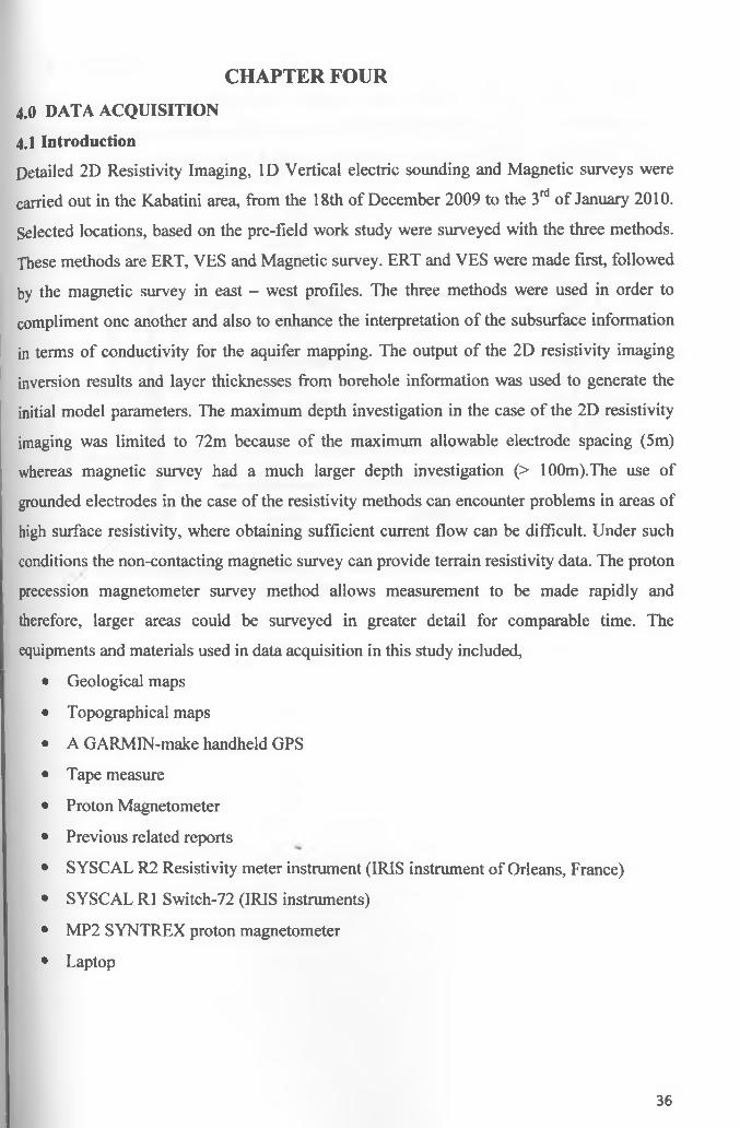
CHAPTER FOUR
4.0 DATA ACQUISITION
4.1 IntroductionDetailed 2D Resistivity Imaging, ID Vertical electric sounding and Magnetic surveys were
carried out in the Kabatini area, from the 18th o f December 2009 to the 3rd o f January 2010.
Selected locations, based on the pre-field work study were surveyed with the three methods.
These methods are ERT, VES and Magnetic survey. ERT and VES were made first, followed
by the magnetic survey in east - west profiles. The three methods were used in order to
compliment one another and also to enhance the interpretation o f the subsurface information
in terms of conductivity for the aquifer mapping. The output o f the 2D resistivity imaging
inversion results and layer thicknesses from borehole information was used to generate the
initial model parameters. The maximum depth investigation in the case o f the 2D resistivity
imaging was limited to 72m because o f the maximum allowable electrode spacing (5m)
whereas magnetic survey had a much larger depth investigation (> 100m).The use o f
grounded electrodes in the case o f the resistivity methods can encounter problems in areas of
high surface resistivity, where obtaining sufficient current flow can be difficult. Under such
conditions the non-contacting magnetic survey can provide terrain resistivity data. The proton
precession magnetometer survey method allows measurement to be made rapidly and
therefore, larger areas could be surveyed in greater detail for comparable time. The
equipments and materials used in data acquisition in this study included,
• Geological maps
• Topographical maps
• A GARMIN-make handheld GPS
• Tape measure
• Proton Magnetometer
• Previous related reports
• SYSCAL R2 Resistivity meter instrument (IRIS instrument o f Orleans, France)
• SYSCAL R1 Switch-72 (IRIS instruments)
• MP2 SYNTREX proton magnetometer
• Laptop
36

4.2 Field surveys
Field work involved surveying of the Kabatini aquifer using Vertical Electrical Sounding,
Electrical Resistivity Imaging (Tomography) and Proton Magnetic Survey. The three surveys
were carried out on four profiles aligned in the east - west direction as shown in fig 4 .land
4.2.
Figure 4.1: The Map showing profiles of Vertical electrical resistivity (VES) and Electrical resistivity tomography (ERT) in Kabatini aquifer
37

Figure 4.2: The map showing the profiles A-B, C-D, E-F and G-H carried in Kabatini aquifer.
The Electrical resistivity tomography and Magnetic survey were carried out along the four
profiles in the East-West direction.
4.2.1 Instrumentation
4.2.2 Vertical electrical sounding (VES) instrumentation
SYSCAL R2 Resistivity meter instrument (IRIS instrument of Orleans, France) was used for
collecting field data for vertical electrical sounding. This is a high powered fully automatic
resistivity meter designed for DC electrical resistivity surveys. It is operated using two power
supplies which includes internal supply for the electronic circuits and external supply for
ground energizing. The internal power supply consists of six 1.5 volts sized dry cells located
at the lower site of the equipment. External power supply in the present study was a 12 volts
car battery whose voltage was stepped up using a 250W DC/DC converter.
SYSCAL R2 is driven by the operator through easy-to-use interactive menus. Only a few
keys control the operation of the instrument at each new reading. The following steps are
followed during the operation of the equipment to acquire data.
38

1. Strike SPACING to enter the wire lines lengths
2. Strike START to inject current and continuously display the current I, voltage V, standard
deviation q and number o f stacks #
3. Strike STOP to terminate the injection o f current.
4. Strike RESULT to compute and display the average value o f resistivity RHO and o f its
standard deviation
5. Strike STORE to save the data.
In electrical resistiv ity survey; O hm s law provides the relationship betw een electric fie ld and current
density and it states that
Where: o = C on d u ctiv ity (a constant)
For an isotropic m edium , the con d u ctiv ity w ill be a scalar quantity so that J and E w ill be in the sam e
direction. For anisotropic m edium , the con d u ctiv ity is a tensor o f secon d rank Oy so that
The subscript i and j m ay be any o f the X , Y , or Z spatial d irections. T he b asis o f all resistiv ity
prospecting w ith direct current is g iven by:
J - CTE (4 .0 )
, (4 .1 )
Yo, W = 0(4 .2 )
In the isotropic ca se Eq4.2_reduces to L ap lace’s equation
Y*V = 0 (4 .3 )
f°r a horizontal earth m odel the so lu tion to Eq._4.3 accord ing to S tefan esco e t a l. (1 9 3 0 ) b ecom es
(4 .4 )
39

Where, J0 = F- is the zero order Bessel function o f the first kind and 0„, is called the kernel function
which is a function o f the thickness and reflection coefficient for an assumed earth model.
By differentiating 4 .4 , the Schlum beger apparent resistivity over an n- layered earth becom es
pjr) = p I * 2 r;J X 0 „(X)J,(Xr)dX.(4 .5)
Where, Ji is the first order Bessel function o f the first kind.
The evaluation o f this integral o f Eq. 4.5 has been done in a number o f ways. In this study w e have
adopted, Ghosh (1971) in which it is possible to determine a linear digital filter, which converts
resistivity transform sam ples into apparent resistivity values for theoretical models.
4.2.2.1 Vertical electrical sounding field measurement
A total o f 16 vertical electrical soundings were carried out using Schlumbeger electrode
configuration. Four profiles A- B , C- D, E - F G- H were located in the East - West direction (see fig.
4.2a). Each profile was separated from the adjacent profile by an interval o f 50 meters. Sounding
stations along the profile were also 50m apart. The direction o f the profiles was selected depending on
how open the terrain was to allow for a wider A B /2 electrode spread. East to west direction was found
to be appropriate since it perpendicular to the principal structures in the area.
Figure 4.2a: The figure showing the Vertical electrical sounding field stations.
40
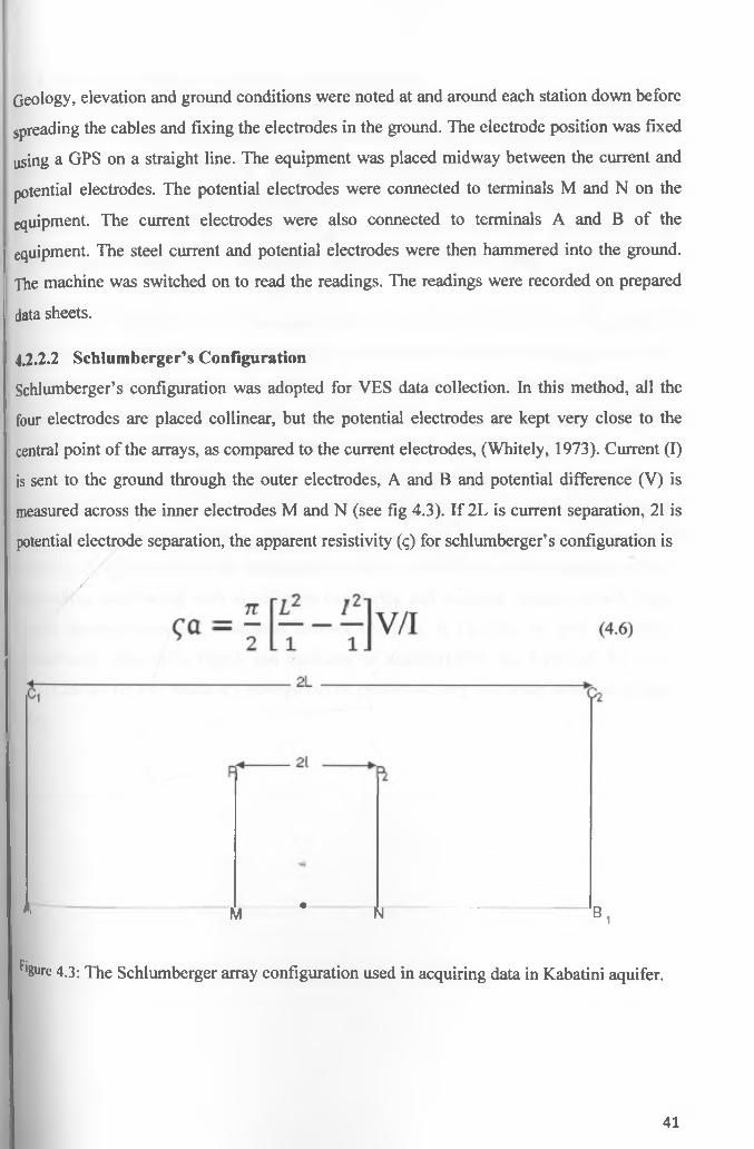
Geology, elevation and ground conditions were noted at and around each station down before
spreading the cables and fixing the electrodes in the ground. The electrode position was fixed
using a GPS on a straight line. The equipment was placed midway between the current and
potential electrodes. The potential electrodes were connected to terminals M and N on the
equipment. The current electrodes were also connected to terminals A and B o f the
equipment. The steel current and potential electrodes were then hammered into the ground.
The machine was switched on to read the readings. The readings were recorded on prepared
data sheets.
4.2.2.2 Schlumberger’s Configuration
Schlumberger’s configuration was adopted for VES data collection. In this method, all the
four electrodes are placed collinear, but the potential electrodes are kept very close to the
central point o f the arrays, as compared to the current electrodes, (Whitely, 1973). Current (I)
is sent to the ground through the outer electrodes, A and B and potential difference (V) is
measured across the inner electrodes M and N (see fig 4.3). If 2L is current separation, 21 is
potential electrode separation, the apparent resistivity (q) for schlumberger’s configuration is
/
*1 ---- ------- M * N B,
hgure 4.3: The Schlumberger array configuration used in acquiring data in Kabatini aquifer.
41

4.2.3 Electrical resistivity tomography instrumentation
The 2D Resistivity data were recorded using the ERT (Electrical Resistivity Tomography).
The complete system consists o f the ERT instrument console, the Swift interface box (the
electronic switching unit),ERT to 12V battery communication cable, ERT to AB,MN cable,
ERT - electrode cables connectors and stainless steel electrode stakes. The ERT can be used
in four basic modes, namely the Manual, Automatic, User and PC modes. More information
on these can be obtained from the Instruction Manual (RES2DINV, 2000).
SYSCAL R1 SWITCH PLUS-72 is a new all-in-one multinode resistivity imaging system. It
features an internal switching board for 72 electrodes and an internal 200W power source.
The output current is automatically adjusted (automatic ranging) to optimize the input voltage
values and ensure the best measurement quality. The system is designed to automatically
perform pre-defined sets o f resistivity measurements with roll-along capability. Four strings
of cable with 18 electrode take-out each are connected together on the back o f the resistivity
meter. Made o f heavy duty seismic cable (see fig 4.5), these strings are composed o f standard
5 m electrode spacing. Compact, easy-to-use and field proof, the SYSCAL R1 Switch-72
measures both resistivity and chargeability (IP). It is ideal for environmental and civil
engineering applications such as pollution monitoring and mapping, salinity control, depth-
to-rock determination and weathered bedrock mapping. It can also be used for shallow
groundwater exploration (depth and thickness o f aquifers).With the SYSCAL R1 PLUS
SWITCH-72 (fig 4.4) resistivity surveys can be performed very efficiently with one operator
only.
42

Figure 4.4: The figure shows Electrical resistivity tomography (ERT) equipment and the style on how the cable is attached to the electrode fixed in the ground.
A■ J..
Electroce strings #1-2
>■» ■■■ ■ «'» ■ ■—«
Electroce strings #3-4(36 take out) 1 = --------- 1 (36 take cut)
: 1
Figure 4.5 Field lay out for the ERT equipment in relation to the cables and electrodes
4.2.3.1 Electrical resistivity tomography data acquisitionA multi-electrode resistivity imaging system, SYSCAL R1 PLU Switch-72 of IRIS-make was
used for the present study. A GARMIN-make handheld GPS was used to position location of
all the electrodes. A total of four resistivity tomography profiles (Figure 4.2) were designed
in the East to West direction. The separation of one electrode to another in the same profile
was 5 mt. Resistivity data were collected using Wenner-Schlumberger array configuration
with inter-electrode spacing of 5 m, during the survey.
43

Figure 4.6: The author setting up ERT equipment to collect 2D resistivity image.
Topographic corrections and 2D inversion model measurements were made using the
inversion algorithm proposed by Loke and Barker, (1996). For uniformity in the
interpretation of different true resistivity sections along various profiles, a common colour
code has been evolved and adopted for presentation of the results. The adopted colour code
answers the key parameters of the aquifer characteristics, like the presence of low resistive
clay/clayey sand horizons, demarcation of locked groundwater pockets, demarcation of the
underground river boundary and identification of boulders and debris. The main factors that
determined daily progress included the battery’s power supply, the weather condition (rain
and thunderstorms) and terrain accessibility (obstructions). After a successful collection of
data from a particular spread, the measured apparent resistivity data was downloaded to a
Laptop. Negative data are automatically removed during this process. The cable and
electrodes were moved to the next-profile. Majority of the survey time was used in the
packing, carrying and laying out the cable.
44
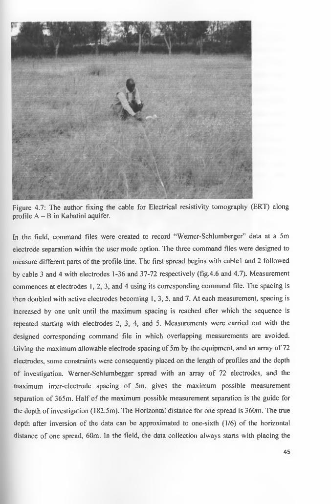
Figure 4.7: The author fixing the cable for Electrical resistivity tomography (ERT) along profile A - B in Kabatini aquifer.
In the field, command files were created to record “Wemer-Schlumberger” data at a 5m
electrode separation within the user mode option. The three command files were designed to
measure different parts of the profile line. The first spread begins with cable 1 and 2 followed
by cable 3 and 4 with electrodes 1-36 and 37-72 respectively (fig.4.6 and 4.7). Measurement
commences at electrodes 1, 2, 3, and 4 using its corresponding command file. The spacing is
then doubled with active electrodes becoming 1, 3, 5, and 7. At each measurement, spacing is
increased by one unit until the maximum spacing is reached after which the sequence is
repeated starting with electrodes 2, 3, 4, and 5. Measurements were carried out with the
designed corresponding command file in which overlapping measurements are avoided.
Giving the maximum allowable electrode spacing of 5m by the equipment, and an array of 72
electrodes, some constraints were consequently placed on the length of profiles and the depth
of investigation. Wemer-Schlumberger spread with an array of 72 electrodes, and the
maximum inter-electrode spacing of 5m, gives the maximum possible measurement
separation of 365m. Half of the maximum possible measurement separation is the guide for
the depth of investigation (182.5m). The Horizontal distance for one spread is 360m. The true
depth after inversion of the data can be approximated to one-sixth (1/6) of the horizontal
distance of one spread, 60m. In the field, the data collection always starts with placing the
45

stainless steel electrode stakes into the ground at intervals of 5m along selected lines. The
swift cables are then laid out on the ground and a clip is used to fix the cable to the electrode,
making sure that there is an electrical contact between them. The cables of electrodes 36 and
37 are then connected to the SYSCAL R1 PLUS SWITCH 72. The SYSCAL RI PLUS
SWITHC 72 and the DC battery are also connected. The details of the traverse from which
data is to be collected are entered into the SYSCAL RI PLUS SWITCH 72 and made ready
for data collection (fig.4.8). A contact resistance test is run to check for poorly connected
electrodes or abnormally high contact resistance reading. The actual measurement was
carried out after the contact resistance test output gave good results, otherwise, the causative
electrode(s) were checked and properly connected or watered some more. It took between
1.00 to 1.30 hours to complete one spread, so during the data collection period a new survey
section was prepared for the next spread. The start and end locations of survey lines were
mapped with a Global Positioning System (GPS). The Resistivity Imaging lines were carried
out more or less along the Proton precession Magnetic survey profiles.
Fig 4.8: The author entering data in SYSICAL RI PLUS SWITCH 72 in Kabatini aquifer.
The ERT algorithm used is based on an Occam’s type inversion that yields a minimum
roughness solution consistent with the data and their errors. The 2-D algorithm, based on a
46
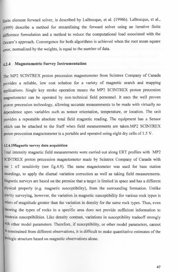
finite element forward solver, is described by LaBrecque, et al. (1996b). LaBrecque, et al.,
(1999) describe a method for streamlining the forward solver using an iterative finite
difference formulation and a method to reduce the computational load associated with the
Occam’s approach. Convergence for both algorithms is achieved when the root mean square
error, normalized by the weights, is equal to the number o f data.
4.2.4 Magnetometric Survey Instrumentation
The MP2 SCINTREX proton precession magnetometer from Scintrex Company o f Canada
provides a reliable, low cost solution for a variety o f magnetic search and mapping
applications. Single key stroke operation means the MP2 SCINTREX proton precession
magnetometer can be operated by non-technical field personnel. It uses the well proven
proton precession technology, allowing accurate measurements to be made with virtually no
dependence upon variables such as sensor orientation, temperature, or location. The unit
provides a repeatable absolute total field magnetic reading. The equipment has a Sensor
which can be attached to the Staff when field measurements are taken.MP2 SCINTREX
proton precession magnetometer is a portable and operated using eight dry cells o f 1.5 V.
4.2.4.1 Magnetic survey data acquisition
Total intensity magnetic field measurements were carried out along ERT profiles with MP2
SCINTREX proton precession magnetometer made by Scintrex Company of Canada with
one 1 nT sensitivity (see fig.4.9). The same magnetometer was used for base station
recordings, to apply the diurnal variation correction as well as taking field measurements.
Magnetic surveys are based on the premise that a target is limited in space and has a different
physical property (e.g. magnetic susceptibility), from the surrounding formation. Unlike
gravity surveying, however, the variation in magnetic susceptibility for various rock types is
orders o f magnitude greater than the variation in density for the same rock types. Thus, even
lowing the types o f rocks in a specific area does not provide sufficient information to
constrain susceptibilities. Like density contrast, variations in susceptibility tradeoff strongly
Mth other model parameters. Therefore, if susceptibility, or other model parameters, cannot
^ constrained from different observations, it is difficult to make quantitative estimates o f the
M ogic structure based on magnetic observations alone.
47

In a particular survey, one may need additional constraints that allow him to use the magnetic
observations in a quantitative fashion. This information is derived from other separate data
sets, for example, formation layering from borehole logging. Once one has constrained the
range o f plausible geological models from other observations, he can design a magnetic
survey to estimate the spatial extent o f the structure and its susceptibility by in-lab forward
modeling. In planning the magnetic survey, I had to predict the noise from sources not o f
interest in the survey, estimated the standard deviation o f the random (operator and
instrument) noise, calculate the shape o f the signal (the theoretical anomaly produced by the
assumed source), then decide whether the signal generated by the target o f interest is above
the noise level that allow me to conduct a meaningful interpretation. If the answer is
affirmative, then I had to determine the survey parameters that will produce the best
compromise between cost and data quality. The Magnetic survey orientation in Kabatini area
was in the East - West Profile. Survey was carried out on four profiles at an interval o f 20 m
along each profile (see fig 4.2). The first there profiles on the northern part o f the project area
had a space interval o f 50 meters from each other. MP2 SINTREX proton precession
magnetometer was used to carry out the survey as shown in fig.4.9. Readings taken included
position coordinates altitude, time and magnetic variations in nT/m
48

Fig 4.9: The author taking magnetic data in the field using MP2 SCINTREX proton
precession magnetometer
Precautions taken during Magnetic survey include;
• Ensured that there were no metallic objects in my pockets.
• Made sure that the arrow on the sensor was pointing towards North. The sensors
mounted vertically like a cylindrical drum.
• Chose a base station in an open area, with hopefully not close to any surface and
buried metal objects (no beeps when collecting the data at the base station).
• Made sure that I go back to the base station to collect 3 data points after one
hour, to the least every 2-3 hours.
• Made sure that 1 tune the magnetometer to its largest signal strength (enter 53-
56) to find the largest signal strength (3.0-9.9).
• Made sure that 1 hit [read] and [store] to store the readings.
• Also ensured the voltage of the batteries is always above 8.4v; otherwise the
batteries were changed (9 Size D cells of them).
49

The use o f Magnetic technique for groundwater exploration, though not as wide spread as
other electrical geophysical techniques (DC resistivity and Resistivity imaging) has increased
considerably in recent years. Examples o f its applicability to groundwater exploration include
among others; characterizing local ground water system in arid alluvial environment (Taylor,
et al., 1992) detection of salt or brackish water interfaces in fresh water aquifers and
determination o f hydro stratigraphy (Fitterman and Stewart, 1986).
/
50

CHAPTER FIVE
5.0 DATA PROCESSING, ANALYSIS AND INTERPRETATION
5.1 IntroductionThe data collected from the field was processed individually depending on the method used
to collect this data in the field. Vertical resistivity sounding data was processed using AGI
Earthlmager software. AGI Earthlmager ID is a Windows 32-bit platform based computer
program that interprets one-dimensional (ID) electrical resistivity sounding data and
produces a layered resistivity model that reveals subsurface geology. Resistivity values at
depths 50m, 57m, 100m, 125m, and 150m were produced using SUFFER 8 . Electrical
resistivity tomography data was processed using RES2DINV software. The program
subdivides the subsurface into rectangular blocks. It then determines the resistivity o f these
blocks and produces a pseudo section that coincides with the measurements. Magnetic data
was interpolated and corrected to the pole to remove diurnal variations. This data was then
processed using EULER software. Magnetic anomaly map was produced using SUFFER 32
software.
5.2 Electrical resistivity tomography (ERT) data processing and analysis
RES2DINV software package was employed in the processing o f the resistivity imaging data.
RES2DINV is a computer program designed by Loke, (1997) to invert the “apparent
resistivity” data obtained from electrical imaging surveys into a two-dimensional (2D) “true
resistivity” model o f the subsurface in an automatic and robust manner with minimal input
from the user. The program determines a resistivity model which approximates the measured
data within the limits o f data errors and which is in agreement with all a priori information.
The program first subdivides the subsurface into a number o f rectangular blocks, the
arrangement o f which is loosely tied to the distribution o f the measured data points in the
pseudo-section but it can also be manipulated. It then determines the resistivity o f the
rectangular blocks that will produce an apparent resistivity pseudo-section that agrees with
die actual measurements. It is worth stating that for the same data set, there would be a range
°f equivalent models whose calculated apparent resistivity values would agree with the
Measured values to the same degree. The program minimizes the difference between the
Measured and the calculated apparent resistivity values, but the inversion method also
tempts to reduce other quantities that will produce certain undesired characteristics in the
^suiting model (Loke, 2000, Loke and Barker, 1996)
51

The RES2DINV program uses a forward modeling subroutine (smoothness-constrained
rnethod) to calculate apparent resistivity values and a non-linear least-squares optimization
technique (deGroot-Hedlin and Constable, 1990) for the inversion routine. As indicated
earlier, the optimization method tries to reduce the difference between the calculated and the
measured apparent resistivity values by adjusting the resistivity of the model blocks
(RES2DINV, 2000). The difference between the measured and calculated apparent resistivity
values is given by the root mean- squared (RMS) error.
The raw data were downloaded to a computer where bad data, particularly negative values
were deleted in the process by the program. These raw data files are converted into the
appropriate format (DAT) readable by the inversion software RES2DINV.EXE (see fig 5.1).
The individual (DAT) input files for all the resistivity imaging survey lines were generated
and made ready for inversion into 2D “true resistivity” image in the program. The routine
practice is to open a file o f a particular traverse results, and view the apparent resistivity data
values in a form of profiles for each data level and to eliminate or remove any inherent bad
datum points. The reason for this step was to manually remove bad data points (i.e. obviously
too large or too small compared to the neighboring data points). Though, careful procedures
were adopted in the field, during the data collection, nevertheless, bad data could come from
sources such as, the failure o f the relays at one o f the electrodes, poor electrode-ground
contact due to dry soil, or shorting across the cables due to the very wet ground conditions, if
such data points occur, then they must be removed, else they can influence the final output
model. After editing the input data, inversion of the data set was then carried with least
squares inversion routine. The final output file displayed after inversion was the measured
and the calculated apparent resistivity pseudo-sections and the true resistivity model section.
52
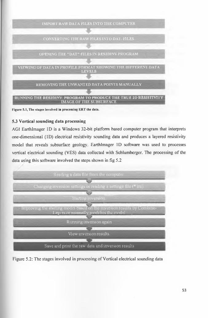
IMPORT RAW DATA FILES INTO THE COMPUTER
CONVERTING THE RAW FILES INTO DAT. FILES
OPENING THE "DAT" FILES IN RES2DINV PROGRAM
VIEWING OF DATA IN PROFILE FORMAT SHOWING THE DIFFERENT DATALEVELS
REMOVING THE UNWANTED DATA POINTS MANUALLY
RUNNING THE RES2DINV. PROGRAM TO PRODUCE THE TRUE 2D RESISTIVITY
Figure S.l, The stages involved in processing ERT the data.
5.3 Vertical sounding data processing
AGI Earthlmager 1D is a Windows 32-bit platform based computer program that interprets
one-dimensional (ID) electrical resistivity sounding data and produces a layered resistivity
model that reveals subsurface geology. Earthlmager ID software was used to processes
vertical electrical sounding (VES) data collected with Schlumberger. The processing of the
data using this software involved the steps shown in fig 5.2
Reading a data file from the computer.
Changing inversion settings or reading a settings file (* ini
Starting inversior■■■■
improving me starting moaei oasea onLayers or manually modifies the model
Running inversion again
View inversion results.
Save and pnnt the raw data and inversion results
Figure 5.2: The stages involved in processing of Vertical electrical sounding data
53
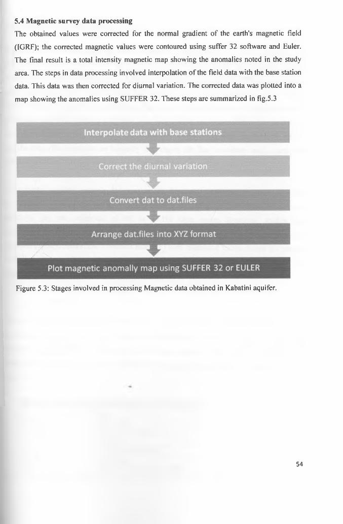
5.4 Magnetic survey data processing
The obtained values were corrected for the normal gradient of the earth's magnetic field
(IGRF); the corrected magnetic values were contoured using suffer 32 software and Euler.
The final result is a total intensity magnetic map showing the anomalies noted in the study
area. The steps in data processing involved interpolation of the field data with the base station
data. This data was then corrected for diurnal variation. The corrected data was plotted into a
map showing the anomalies using SUFFER 32. These steps are summarized in fig.5.3
Figure 5.3: Stages involved in processing Magnetic data obtained in Kabatini aquifer.
54

5.5 Results and geological interpretation
Resistivity is a fundamental electrical property o f rocks, which is closely related to rock
lithology of which the main controlling factors are bulk rock porosity, pore structure, amount
and salinity o f water, temperature and the presence of clays. To convert the resistivity picture
into a geological one requires some knowledge of the typical resistivity values for the
different types o f subsurface materials and geology o f the surveyed area. Though most o f the
geological data from existing boreholes were unavailable, the information obtained from the
available lithological log done by Prof. Mathu near location 0,E along profile A-B showed
that the subsurface materials are basically clay, clayey silt, fine to medium sand, coarse sand,
pebbles, boulders, tuff and lava.
Groundwater quality analysis information on boreholes indicate the mean electrical
conductivity (EC) o f the waters is approximately to 550pS/cm and therefore its mean
resistivity (p), the reciprocal o f EC is 18.181 Ohm meter. Empirical studies have
demonstrated that a correlation exists between F and the particle size (fig.5.4) o f sedimentary
materials (Sporry, 2001) .The formation factor (F) were calculated for the station 0,E near the
boreholes along profile A-B where vertical resistivity sounding surveys was carried out
using the following formula.
F =Pm-
where pf is the resistivity of formation ,and pw is the resistivity o f pore water. This relation
is a derivation from Archie’s Law (Keller and Frischknecht, 1966). The general relationship
between F and grain-sizes established in NW-Europe (Sporry, 2001) has been adopted as a
rough guide, because it fitted well with borehole log and the calculated F values (fig 5.5 and
Table 5.1).
F Grain size1 Clays1.5-2 Sandy clays2-2.5 Silty and clay Sands3 Fine sands4 - 5 Medium coarse sands6 -7 Coarse sands> 8 Very coarse sands and pebbles
figure 5.4: Relationship between F values and grain sizes from various studies in NW Europe
55

Lithological interpretation o f station 0,E according to Archie’s Law
Lithological interpretation according to borehole log done by Prof. Mathu’s on
d e p t h EC pw pf F GRAIN SIZE profile A -B near station 0JE
0.787 550 18.181 40.194 2.210769 Silty and clayey sand
Brownish white loose soils
1.251 550 18.181 46.554 2.560585 Silty and clayey sand
Brownish white loose soils and gravel cemented by clay and ash
1.771 550 18.181 120.162 6.609207 Coarse sand Gravel cemented by clay and ash
3.154 550 18.181 237.341 13.05434 Very coarse sand and pebbles
Brownish white loose soils and gravel cemented by clay and ash
4.931 550 18.181 156.829 8.625983 Very coarse sand and pebbles
Graded coarse sands and gravel cemented by argillaceous material
7.033 550 18.181 61.613 3.388867 Fine sand Loose medium brown graded fine sands
72.911 550 18.181 40.818 2.245091 Clayey sand Pale brownish (buff) tuff with a thin layer o f sediments from 10 - 12 m depth
19.64 550 18.181 67.371 3.705572 Fine sand Loose sediments o f clay (20%), sand (30%) and gravel (30%) with trachyte and phonolite clastsLoose sediments o f clay (20%), sand (30%) and gravel (30%) with trachyte and phonolite clastsMedium dark grey tuff and ash with few hard rock fragments and white patches o f feldspar and ash
34.875 550
/18.181 165.304 9.092129 Very Coarse
sand andr v a U U I a rpe Doles
Dark yellowish tuff with few medium to dark grey patches
59.832 550 18.181 142.246 7.823882 Very Coarse sand and pebbles
Weathered erosional horizon followed immediately by dark almost black basalt rock composed o f a layer dominated by mafic minerals and subordinate quartz, Medium to slightly dark grey volcanic ash with lapith fragments (approx. 1 - 2 cm in size), Light grey pumiceous horizon with few rounded loose gravels, Medium grey rhyolite with obsidic fragments, Light tunic white tuff, Loose to cemented rounded clasts omposed o f pumice pebbles, sands and occasionally cemented by brownish mud, Dark grey to black, tough moderately weathered rock with glassy sandstone phenocrysts, Brownish weathered rounded clasts o f dark grey to black phonolite Medium grey highly felsic trachyte (tough rock)
106.905 550 18.181 67.764 3.727188 Fine sand Greyish white tuff
165 > 550 18.181 21.759 1.196799 Clays Greyish white tuff, not strongly indurated, and mixed with redish mud
figure 5.5: F values o f BH 8 in Kabatini aquifer which is located on the profile A - B (see fig-4.2)
56
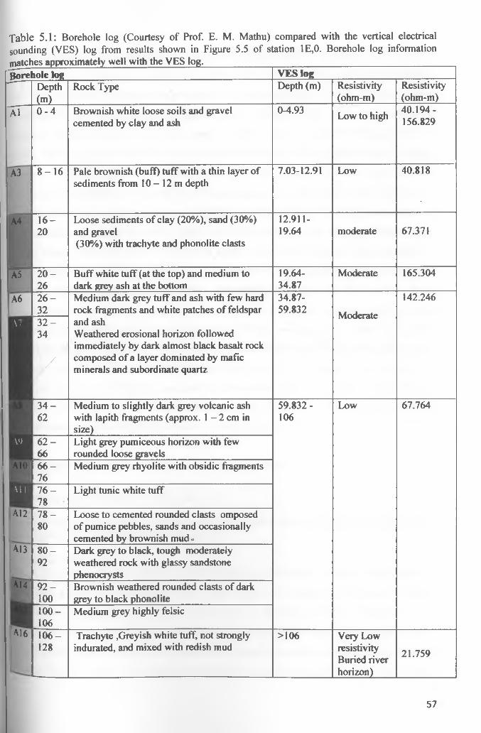
Table 5.1: Borehole log (Courtesy of Prof. E. M. Mathu) compared with the vertical electrical sounding (VES) log from results shown in Figure 5.5 of station 1E,0. Borehole log information matches approximately well with the VES log. ________ _______________________________B ore liole log V E S lo g
" Depth Rock Type Depth (m) Resistivity Resistivity(m) (ohm-m) (ohm-m)
A1 0 -4 Brownish white loose soils and gravel 0-4.93 Low to high 40.194-cemented by clay and ash 156.829
A3 8 -1 6 Pale brownish (buff) tuff with a thin layer of sediments from 10 - 12 m depth
7.03-12.91 Low 40.818
A4 1 6 - Loose sediments of clay (20%), sand (30%) 12.911-20 and gravel 19.64 moderate 67.371
(30%) with trachyte and phonolite clasts
A5 2 0 - Buff white tuff (at the top) and medium to 19.64- Moderate 165.30426 dark grey ash at the bottom 34.87
A6 2 6 - Medium dark grey tuff and ash with few hard 34.87- 142.24632 rock fragments and white patches of feldspar 59.832 Moderate
\ 7 3 2 - and ash34 Weathered erosional horizon followed
immediately by dark almost black basalt rock
/composed of a layer dominated by mafic minerals and subordinate quartz
3 4 - Medium to slightly dark grey volcanic ash 59.832 - Low 67.76462 with lapith fragments (approx. 1 - 2 cm in
size)106
\‘> 6 2 - Light grey pumiceous horizon with few66 rounded loose gravels
A10 6 6 - Medium grey rhyolite with obsidic fragments76
\ M 7 6 - Light tunic white tuff78
A12 7 8 - Loose to cemented rounded clasts omposed80 of pumice pebbles, sands and occasionally
cemented by brownish mud -A13 8 0 - Dark grey to black, tough moderately
92 weathered rock with glassy sandstone phenocrysts
A14 9 2 - Brownish weathered rounded clasts of dark100 grey to black phonolite100- Medium grey highly felsic
A16106106- Trachyte ,Greyish white tuff, not strongly >106 Very Low128 indurated, and mixed with redish mud resistivity
Buried river horizon)
21.759
57

The aim of geological interpretation o f resistivity sounding data is to determine the thickness
and resistivity o f different horizons from a study o f the Vertical Electrical Sounding (VES)
field curves and to use these results to obtain a complete geological picture o f the area under
investigation. The Vertical Electrical Sounding data obtained in this work was analyzed by
using the Zohdy’s method (1989) and computer based inversion using Earthlmager software,
which allows the performance of automatic interpretation o f the Schlumberger sounding
curves to obtain the equivalent n-layer model from the apparent resistivity curve o f each
sounding. This procedure was used for all the sounding points obtained in the study area, in
order to obtain the equivalent apparent resistivity models o f each sounding, their depths as
well as thicknesses. Different curve types were identified in the area showing different geo
electric layers. These layers are o f different shapes and characteristics which is typified by
the formation. The numerous layers that were generated by the computer were grouped into
relevant geologic depth intervals called geo-electric sections and the resulting layer
parameters were then given geologic interpretation. The type o f curves, the resistivity o f the
sediments and the lithological logs from nearby boreholes were used in conjunction with the
knowledge o f the local geology o f the study as guides in the interpretation and analysis o f the
geologic section in terms of shallow structures and buried river channels. The knowledge of
the local geology o f Kabatini was used in constructing the earth model. The lithology
indicates broadly that within the depth penetrated; the succession is clay, clay silt, and fine to
medium sand, coarse sand, pebbles, boulders, tuffs and lava.
5.5.1 Interpretation of Vertical electrical sounding results
1. Analysis of VES stations on profile A - B
Profile A -B is located on the northern part (latitude 9971210) o f the study area and consists of stations (1 W, 0), (0, 0), (1 E, 0) and (2E, 0)
a Station 1W,0Layers 1-3 have moderate resistivity values between 56.369 and 87.823 ohm meter. There is
311 ascending trend in the resistivity values from the surface to layer 5. The resistivity values
toon decline abruptly from 145.373 on layer five to 76.099 and 45.05 of layers 6 and 7
^spectively. Layer 8 and 9 shows an increase in the resistivity values which declines again
°n layers 10, 11 and 12. The curve indicates two conductive layers, o f which one is confined
')ehveen layers 5 and 8 . The other conductive layer begins from layer 10 to the layer 12(see
58

fig.5.6 and table 5.2). The thickness o f layer 12 cannot be determined because it occurs at the
bottom. The curve shows a combination o f K - H - K
KMM)
l(M)
EaI
•V,
Measured and Modeled Data
_
—h
1
t —
I K)S c h lu m b e rg c r A rray . A B /2 (m )
Iteration = 2 RM S = 4.77%
IIM)
Layered Resistivity Model
165.00
Depth (n t)
Figure 5.6: Resistivity values o f layered earth model for station 1W,0 along profile A -B
Table 5.2: Table shows the layer thickness and resistivity for station 1 W,0
Layersequencefrom
surface
Numberoflayers
Depth(meters)
Thickness(meters)
Resistivity(ohmmeter)
1 0-1 0.168 0.168 56.3692 1-2 0.462 0.294 69.4413 2-3 1.118 0.656 87.8234 3-4 2.102 0.984 115.6975 4-5 3.848 1.746 145.3736 5-6 5.883 2.035 76.0997 6-7 9.933 4.05 45.0578 7-8 14.965 5.032 116.4389 8-9 28.121 13.156 183.4710 9-10 38.321 10.2 47.60911 10-11 75.734 37.413 49.3712 11-12 > 75.734 > 89.266 38.186
59

1). Station 0,0The first layer of station (0,0) consist of very low resistivity material which could be clay saturated
with water. Resistivity values for layers 2,3,4 and 5 are 20.1,44.3,215.1 and 657.5 ohm meter
respectively. There is an ascenting trend of the curve for this layers. The values of layers 6,7,8, and 9
show descenting trend of the resitivity values indicating the shallow strucutres containing low
resistivity at a depth of 15m. The inversion curves of K-H-K is observed in this station (fig. 5.7).
•7.
1as
1000
100
/ 'V,
Measured and Modeled Data
I 10Sclilum berger A rray . A B /2 (m )
Itera lion = I RM S = 6.37%
100
Layered Resistivity Model
165(H)1 Depth (m )
Figure 5.7: Resistivity values o f layered earth model from station 0, 0 along profile A -B
Table 5.3: Table shows the layer thickness and resistivity for station 0,0
Layersequencefromsurface
Numberoflayers
Depth(meters)
Thickness(meters)
Resistivity(ohmmeter)
1 0-1 0.11 0.11 12.0512 1-2 0.374 0.264 20.1183 2-3 ** 0.646 0.272 44.3034 3-4 0.868 0.222 215.0835 4-5 2.465 1.597 657.496 5-6 4.3 1.835 306.8777 6-7 5.736 1.436 65.3778 7-8 17.33 11.594 42.5389 8-9 29.304 11.974 89.84910 9-10 56.09 26.786 179.79211 10-11 81.084 24.994 78.81412 11-12 > 81.084 >83.916 30.881
6 0
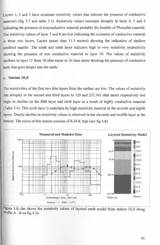
Layers 1, 2 and 3 have moderate resistivity values that indicate the presence o f conductive
materials (fig 5.7 and table 5.3). Resistivity values increases abruptly in layer 4, 5 and 6
indicating the presence o f nonconductive material probably the boulder o f Phonolite material.
The resistivity values o f layer 7 and 8 are low indicating the existence o f conductive material
in these two layers. Layers (more than 11.5 meters) showing the indication o f shallow
confined aquifer. The ninth and tenth layer indicates high to very resistivity respectively
showing the presence o f non conductive material in layer 10. The values o f resistivity
declines in layer 11 from 78 ohm meter to 30 ohm meter showing the presence o f conductive
body that goes deeper into the earth.
c. Station 1E,0
The resistivities o f the first two thin layers from the surface are low. The values o f resistivity
rise abruptly in the second and third layers to 120 and 237.341 ohm meter respectively and
begin to decline on the fifth layer and sixth layer as a result o f highly conductive material
(Table 5.4). This sixth layer is underlain by high resistivity material in the seventh and eighth
layers. Drastic decline in resistivity values is observed in the eleventh and twelfth layer at the
bottom. The curve o f this station consists o f K-H-K type (see fig 5.8).
Measured and Modeled Data Layered Resistivity Model1000
7. •7.j
OH5‘d
1(H)
'V,-_
I 10Schlumbereer A rray . A B 2 (m )
Iteration = .3 RM S = 3.47%
1(H)
34.87
59.83
106.91
165.00
Depth ( in )
^gure 5.8, the shows the resistivity values o f layered earth model from station 1E,0 along Profile A -B on fig 4.2a
61
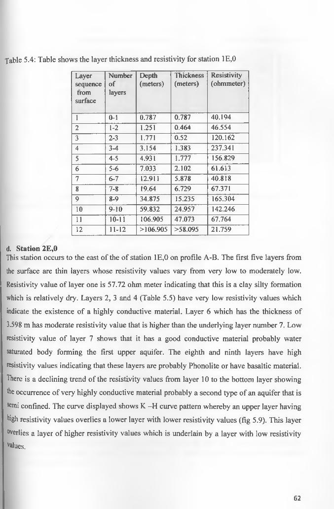
fable 5.4: Table shows the layer thickness and resistivity for station 1E,0
Layersequencefromsurface
Numberoflayers
Depth(meters)
Thickness(meters)
Resistivity(ohmmeter)
1 0-1 0.787 0.787 40.1942 1-2 1.251 0.464 46.5543 2-3 1.771 0.52 120.1624 3-4 3.154 1.383 237.3415 4-5 4.931 1.777 156.8296 5-6 7.033 2.102 61.6137 6-7 12.911 5.878 40.8188 7-8 19.64 6.729 67.3719 8-9 34.875 15.235 165.30410 9-10 59.832 24.957 142.24611 10-11 106.905 47.073 67.76412 11-12 >106.905 >58.095 21.759
d. Station 2E,0This station occurs to the east o f the o f station 1E,0 on profile A-B. The first five layers from
the surface are thin layers whose resistivity values vary from very low to moderately low.
Resistivity value o f layer one is 57.72 ohm meter indicating that this is a clay silty formation
which is relatively dry. Layers 2, 3 and 4 (Table 5.5) have very low resistivity values which
indicate the existence o f a highly conductive material. Layer 6 which has the thickness o f
3.598 m has moderate resistivity value that is higher than the underlying layer number 7. Low
resistivity value o f layer 7 shows that it has a good conductive material probably water
saturated body forming the first upper aquifer. The eighth and ninth layers have high
resistivity values indicating that these layers are probably Phonolite or have basaltic material.
There is a declining trend of the resistivity values from layer 10 to the bottom layer showing
the occurrence o f very highly conductive material probably a second type o f an aquifer that is
fcmi confined. The curve displayed shows K -H curve pattern whereby an upper layer having
high resistivity values overlies a lower layer with lower resistivity values (fig 5.9). This layer
°verlies a layer o f higher resistivity values which is underlain by a layer with low resistivity
values.
62

Measured and Modeled DataHXNI
“1as
KM)
% __
■H----------H-----TT
Layered Resistivity ModelOp
14..t o |
1 10 I00S c h lu m b c rg c r A rray . A B 2 (m l
Ite ra tio n = I R M S = 2 .2 1 %
1.14.44
165.00
D ep th (ill)
Figure 5.9, the figure shows the resistivity values o f layered earth model from station 2E, 0 along profile A -B on fig 4.2a. *•
Table 5.5: Table shows the layer thickness and resistivity for station 2E,0
Layersequencefromsurface
Numberoflayers
Depth(meters)
Thickness(meters)
Resistivity(ohmmeter)
1 0-1 0.403 0.403 57.7252 1-2 0.708 0.305 19.2723 2-3 1.237 0.529 10.4714 3-4 1.981 0.744 12.1795 4-5 2.625 0.644 75.8746 5-6 6.223 3.598 99.7027 6-7 14.394 8.171 36.8848 7-8 20.201 5.807 123.3929 8-9 32.65 12.449 187.97310 9-10 42.177 9.527 51.82811 10-11 134.443 92.266 30.91412 11-12 >134.443 >30.557 26.258
*• Analysis of Profile C-Dprofile occurs to the south o f profile A - B along latitude 991160. The profile runs in the
^ t to west direction and contains VES stations (1 W ,1 S),(0,1S),(1E,1S) and (2E,1S) whose ^ordinates are listed in table 4.1a
63
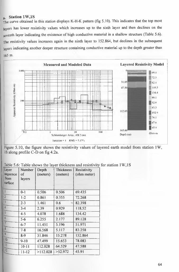
a. Station 1W,1SThe curve obtained in this station displays K-H-K pattern (fig 5.10). This indicates that the top most
layers has lower resistivity values which increases up to the sixth layer and then declines on the
seventh layer indicating the existence of high conductive material in a shallow structure (Table 5.6).
flie resistivity values increases again in the ninth layer to 152.864, but declines in the subsequent
layers indicating another deeper structure containing conductive material up to the depth greater than
165 m.
Measured and Modeled Data
5I1
lOOOr
100 '
'*T
—
I loSchlum berecr A rray . A B 2 (m )
Iteration = I RM S = 5.13%
l (M)
Layered Resistivity Model
Depth ( in )
1 6<M 1 72.3
Z 82 .4
: i i x 5
g 1.34.4
S‘).l
1 5 2 .0
83.3
| 152.9
| 78.1
1 4 7 .6
1 45.9
O hm -m
Figure 5.10, the figure shows the resistivity values o f layered earth model from station 1W, IS along profile C-D on fig 4.2a.
Table 5.6: Table shows the layer thickness and resistivityLayersequencefromsurface
Numberoflayers
Depth(meters)
Thickness(meters)
Resistivity (ohm meter)
1 0-1 0.506 0.506 69.4352 1-2 0.861 0.355 72.2683 2-3 1.461 0.6 82.3984 3-4 2.39 0.929 118.525 4-5 4.078 1.688 134.426 5-6 6.255 2.177 89.128T 6-7 11.451 5.196 51.971t —— 7-8 16.568 5.117 83.2589 8-9 31.846 15.278 152.86410" " 9-10 47.499 15.653 78.083i T " — 10-11 112.028 64.529 47.588
[12T~~ 11-12 >112.028 >52.972 45.91
for station 1 W,1S
64

b. Station 0,1S
The type o f the curve observed in this station is a combination o f Q-H-A (fig 5.11) indicating
very high resistivity values on the bottom layer. The first layer on the top has high resistivity
value o f 140.88 ohm meter (Table 5.7). The resistivity values drops abruptly to 14.542 ohm
meter in the second layer. The resistivity values increases slowly on the third, fourth and fifth
layer and then begins dropping again on the sixth, seventh and eighth layer. The eighth layer
whose thickness is 25.15 m thick has a low resistivity value o f 20.05 ohm meter signifying
the existence o f conductive material which is a confined aquifer in shallow structure.
Resistivity values begin to increase on the ninth layer reaching a maximum of 708.9 ohm
meter on the tenth layer. The tenth layer has a thickness that is greater than 210 m which
indicates that this layer could be part o f an intrusion within the study area.
Measured and Modeled Data
Itera tion = 8 RM S = 1.83%
Layered Resistivity Model !
><*<•<* w — ; w <-!>••< v* i •Pi.L .i Sit. A uM &fS ’M»:V4kiU ^ R kS m m I K jfcitihmtm lbD **H « S<OtTDAl_______________________________
figure 5.11, the figure shows the resistivity values o f layered earth model from station 0,1S along profile C-D on fig 4.2a
65

Table 5.7: Table shows the layer thickness and resistivity for station 0,1S
Layersequencefromsurface
Numberoflayers
Depth(meters)
Thickness(meters)
Resistivity(ohmmeter)
1 0-1 0.702 0.702 140.8882 1-2 0.851 0.149 14.5423 2-3 1.983 1.132 38.3494 3-4 7.111 5.128 46.6525 4-5 7.947 0.836 59.5476 5-6 9.619 1.672 39.3147 6-7 12.792 3.173 27.5328 7-8 37.942 25.15 20.0529 8-9 48.828 10.886 38.62710 9-10 >48.828 > 201.172 708.861
c. Station IE,IS
This station is found on the second profile C-D, which occurs to the south o f profile A-B.
The first layer has very high resistivity values (444.7 Ohm meter) indicating the presence
of unweathered Phonolite, the values o f resistivity drops significantly in the second and
third layers. The third layer is underlain by a relatively high resistivity value layer which
overlies a fifth low resistivity value layer at a depth o f 3.77 to 6.844 m (Table 5.8). The
resistivity values for the sixth and seventh layer increases abruptly but declines on the
subsequent layers till it reaches very low resistivity value o f 16.33 ohm meter on the
bottom layer. The Q-H-Q type curve is noted in this station (fig 5.12).
66
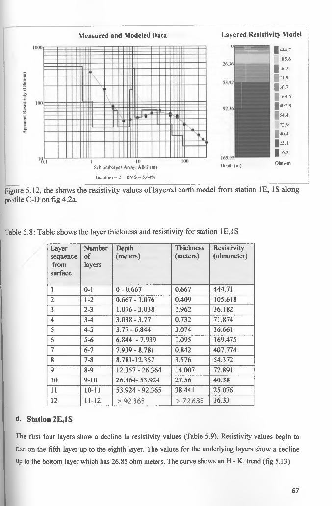
1 44 4 .7
105.6
1 36 .2
| 7 1 . 9
| 3 6 . 7
5 169.5
1 4 0 7 .8
1 5 4 .4
j 7 2 . 9
1 4 0 4
| 2 5 ,
1 16.3
O h m -inS c h lu m b e rg c r A rray . A B 2 (m ) D ep th (m )
Ite ra tio n “ 2 R M S = 5 .6 4 %
Figure 5.12, the shows the resistivity values o f layered earth model from station IE, IS along profile C-D on fig 4.2a.
Measured and Modeled Data Layered Resistivity Model
Table 5.8: Table shows the layer thickness and resistivity for station IE ,IS
Layersequencefromsurface
Numberoflayers
Depth(meters)
Thickness(meters)
Resistivity(ohmmeter)
1 0-1 0 - 0.667 0.667 444.712 1-2 0.667- 1.076 0.409 105.6183 2-3 1.076-3.038 1.962 36.1824 3-4 3.038-3.77 0.732 71.8745 4-5 3.77 - 6.844 3.074 36.6616 5-6 6.844 - 7.939 1.095 169.4757 6-7 7.939-8.781 0.842 407.7748 7-8 8.781-12.357 3.576 54.3729 8-9 12.357-26.364 14.007 72.89110 9-10 26.364- 53.924 27.56 40.3811 10-11 53.924 - 92.365 38.441 25.07612 11-12 > 92.365 > 72.635 16.33
d. Station 2E,1S
The first four layers show a decline in resistivity values (Table 5.9). Resistivity values begin to
rise on the fifth layer up to the eighth layer. The values for the underlying layers show a decline
up to the bottom layer which has 26.85 ohm meters. The curve shows an H - K. trend (fig 5.13)
67

Measured and Modeled Data Layered Resistivity Model
IIHHI
77
Hft
100
'V,
5■u.
1 10Schlum bcrgcr A rray. A B 1 (n i)
Iteration = I RMS = 3.9K%
IOO 165 .00
Depth (tit)
Figure 5.13, the shows the resistivity values o f layered earth model from station 2E,1S along profile C-D on fig 4.2a.
Table 5.9: Table shows the layer thickness and resistivity for station 2E,1S
Layersequencefromsurface
Numberoflayers
Depth(meters)
Thickness(meters)
Resistivity(ohmmeter)
1 0-1 0.417 0.417 268.0382 1-2 0.632 0.215 126.6373 2-3 0.881 0.249 56.4594 3-4 1.911 1.03 27.8135 4-5 3.516 1.605 31.9896 5-6 5.176 1.66 60.1037 6-7 7.952 2.776 192.1748 7-8 15.565 7.613 213.5989 8-9 26.605 11.04 108.4710 9-10 51.007 24.402 63.48111 10-11 94.191 43.184 58.112 11-12 > 94.191 >70.809 26.85
68

3. Analysis of Profile E - F
This profile occurs to the south o f profile C - D along latitude 9971110. The profile runs in
the east to west direction and contains VES stations (1W, 2S), (0, 2S), (IE , 2S) and (2E, 2S)
whose coordinates are shown in table 4.2a.
a. Station 1W,2S
This station has a resistivity o f 131.433 ohm meter on the upper layer which increases to a
maximum of 433.42 ohm meter in third layer. The resistivity values then decline steadily up
to 63.73 ohm meter on the ninth layer (Table 5.10). The ninth layer has a thickness o f 23.346
m thick with moderate resistivity because o f having relatively high conductive material at a
depth o f 45.49 m from the surface. The resistivity values o f the tenth layer increases to
118.937 ohm meter, but the drops gradually on the eleventh layer. Bottom layer has got very
low resistivity as compared with the resistivity o f the layers above it. The curve obtained in
this station is a K -Q curve (fig. 5.14)
M ea su red an d M od eled D ata L a y ered R esistiv ity M od el
Depth ( in )
I 131 4259 .3
1 433.4
■ 37 3 .6
1 2 7 5 .0
IXX. 5
| 1X2.1
I 108.6
1 6 3 .7
I ll8'9| 100.5
■ 39.X
Ohm-m
l lc ra lio n = 2 R M S 1- 4.12%
figure 5.14, the shows the resistivity values o f layered earth model from station 1W, 2S a*ong profile E -F on fig 4.2a.
69

'fable 5.10: Table shows the layer thickness and resistivity for station 1 W,2 S
Layersequencefromsurface
Numberoflayers
Depth(meters)
Thickness(meters)
Resistivity(ohmmeter)
1 0-1 0.832 0.832 131.4332 1-2 1.172 0.34 259.293 2-3 1.934 0.762 433.424 3-4 3.11 1.176 373.6225 4-5 5.05 1.94 275.0056 5-6 8.827 3.777 188.4977 6-7 15.026 6.199 182.088 7-8 22.144 7.118 108.646
9 8-9 45.49 23.346 63.7310 9-10 74.662 29.172 118.93711 10-11 102.651 27.989 100.52112 11-12 >102.651 >62.349 39.775
b. Station 0,2 S
The first layer o f this station has moderate resistivity which increases gradually up to the fifth
layer which has resistivity values o f 141.208 ohm meter. Layers seven and eight have
moderate resistivity o f 72.024 and 73.539 ohm meter respectively (Table 5.11). There is a
rising trend o f the resistivity values in the ninth to twelfth layer forming K - A (fig. 5.15).
The high resistivity o f 1197.9 ohm meter o f the bottom layer indicates the existence o f an
intrusive material that whose thickness cannot be determined because it is the bottom layer.
70

Measured and Modeled Data Layered Resistivity ModelKHKXI
1000
--7.
■I 100
"A—
I 10S c h lu m b c rg c r A rray . A B 2 (m )
lic ra lio n = 2 R M S = 9.9.1%
l<M> 1.17.50'
D ep th (in ) Ohm -ill
Figure 5.15, the shows the resistivity values o f layered earth model from station 0,2S along profile E-F on fig 4.2a.
Table 5.11: Table shows the layer thickness and resistivity for station 0,2S
Layersequencefrom
surface
Numberoflayers
Depth(meters)
Thickness(meters)
Resistivity(ohmmeter)
1 0-1 0.835 0.835 76.1262 1-2 1.301 0.466 94.2783 2-3 2.026 0.725 115.0224 3-4 3.19 1.164 136.1465 4-5 5.19 2 141.2086 5-6 8.196 3.006 105.3017 6-7 13.103 4.907 72.0248 7-8 20.813 7.71 73.5399 8-9 32.554 11.741 100.2810 9-10 50.65J 18.097 131.0811 10-11 77.84 27.189 233.07212 11-12 >77.84 >59.66 1197.865
c. Station 1E,2S
*e first layer in this station has a very low resistivity value which increases in the second layer
^able 5.12). The resistivity of the third layer indicates clay material overlying the fifth layer that has
dera te resistivity of 84.426 ohm meter. The low resistivity values of the sixth and seventh layer
71

increase to the peak of 169.027 ohm meter in the ninth layer after which the trend declines to 23.546
ohm meter on the twelfth layer. The type of the curve formed in this station is K curve (fig 5.16)
Measured and Modeled Data Layered Resistivity Model
Ite ra tio n = 1 R M S = 4 .2 3 %
Figure 5.16: The figure shows the resistivity values o f layered earth model from station IE, 2S, along profile E -F (fig 4.2a)
Table 5.12: Table shows the layer thickness and resistivity for station IE,2 S
Layersequencefrom
surface
Numberoflayers
Depth(meters)
Thickness(meters)
Resistivity(ohmmeter)
1 0-1 0.384 0.384 12.3242 1-2 0.759 0.375 26.3063 2-3 1.606 0.847 12.084 3-4 2.362 0.756 22.2485 4-5 4.311 1.949 84.426
6 5-6 5.638 1.327 34.3647 6-7 10.856 5.218 28.4448 7-8 14.827 3.971 154.5919 8-9 29.865 15.038 169.02710 9-10 46.138 16.273 53.09511 10-11 100.045 53.907 28.96612 11-12 >100.045 >64.955 23.546
d. Station 2E,2SThe first layer shows moderate resistivity value of 71.483 ohm meter which declines up to 34.657
ohm meter in the fourth layer (Table 5.13). The trend of the resistivity values rises from the fifth
72

layer to the ninth layer. Resistivity values drops gradually from the tenth layer up to 22.119 ohm
meter in the twelfth layer. The type of the curve obtained in the station is the H-K curve (fig
5.17).
Measured and Modeled Data Layered Resistivity Modell(HH)
y."7.
100
'V,
1 3 ,
32.05
51. 1(1
76.XI
I 10S chU tm berger A rray , A B /2 (n t)
d e ra tio n = .3 R M S = 3 .5 1 %
100 165 .00
D ep th (n t)
Figure 5.17, the figure shows the resistivity values o f layered earth model from station 2E, 2 S along profile E-F on fig 4.2a
Table 5.13: Table shows the layer thickness and resistivity for station 2E, 2 S
Layer sequence from surface
Number of layers
Depth(meters)
Thickness(meters)
Resistivity(ohmmeter)
1 0-1 0.338 0.338 71.4832 1-2 0.66 0.322 61.9153 2-3 1.184 0.524 35.984 3-4 2.11 0.926 34.6575 4-5 3.645 1.535 55.2866 5-6 6.879 3.234 62.3627 6-7 12.365 5.486 61.0828 7-8 19.458 7.093 158.5199 8-9 32.047 12.589 206.47710 9-10 51.098 19.051 113.58611 10-11 76.881 25.783 36.98712 11-12 >76.881 >88.119 22.119

4. Analysis of Profile G - H
This profile occurs to the south o f profile E - F along latitude 9971058. The profile runs in the east to west direction and contains VES stations (1 W,3S),(0,3S),(1E,3S) and (2E,3S) whose coordinates are shown in Table 4.2a.
a. Station 1W,3S
The first layer of this station has low resistivity value of 41.42 ohm meter. The trend of resistivity
increases up to 369.573 ohm meter in the fifth layer. The resistivity values then decreases from the
sixth layer which has 234.194 ohm meter to 55.874 ohm meter in eighth layer (Table 5.14). The
values of resistivity increases again slightly to 118.101 ohm meter after which it declines to low
resistivity values of 32.293 ohm meter in the bottom layer. The curve of this station is in the form of
K curve (fig 5.18).
Measured and Modeled Data Layered Resistivity Model
26 .1 3
5 1.96L
9 1 .2 1 i
I65.<MP
D ep th (m )
1 4 1 4
1 6 7 .6
9 4 .4
1 23 8 .2
| 3 6 9 .6
1 234 .2
gj73-41 5 5 .9
101.7
118.1
1 8 1 .6
i-™O h m -n i
Figure 5.18, the shows the resistivity values o f layered earth model from station 1W, 3S along profile G-H on fig 4.2a
74
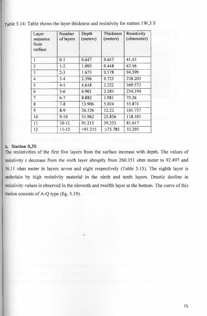
fable 5.14: Table shows the layer thickness and resistivity for station 1 W,3 S
Layersequencefromsurface
Number of layers
Depth(meters)
Thickness(meters)
Resistivity(ohmmeter)
1 0-1 0.647 0.647 41.422 1-2 1.095 0.448 67.563 2-3 1.673 0.578 94.3994 3-4 2.396 0.723 238.2035 4-5 4.618 2.222 369.5736 5-6 6.901 2.283 234.1947 6-7 8.882 1.981 73.368 7-8 13.906 5.024 55.8749 8-9 26.126 12.22 101.73710 9-10 51.962 25.836 118.10111 10-11 91.215 39.253 81.61712 11-12 >91.215 ^73.785 32.293
b. Station 0,3SThe resistivities o f the first five layers from the surface increase with depth. The values of
resistivity r decrease from the sixth layer abruptly from 260.351 ohm meter to 92.497 and
56.11 ohm meter in layers seven and eight respectively (Table 5.15). The eighth layer is
underlain by high resistivity material in the ninth and tenth layers. Drastic decline in
resistivity values is observed in the eleventh and twelfth layer at the bottom. The curve o f this
station consists o f A-Q type (fig. 5.19).
75

Measured and Modeled Data1000
7.'7.rjTS
I
loo-hO-
1---r-»
I 10S c h lu m b c rs e r A rray . A B 2 o n )
Ite ra tio n 1 R M S = 4 .8 6 %
=cq
100
Layered Resistivity Model
165.00
D ep th (m l
Figure 5.19, the shows the resistivity values o f layered earth model from station 0,3S along profile G-F on fig 4.2a
Table 5.15: Table shows the layer thickness and resistivity for station 0,3 S
/Layersequencefromsurface
Numberoflayers
Depth(meters) Thickness(meters)
Resistivity (ohm meter)
1 0-1 0.444 0.444 57.452 1-2 0.813 0.369 105.5893 2-3 1.648 0.835 128.1664 3-4 2.851 1.203 150.2945 4-5 4.495 1.644 269.7166 5-6 7.047 2.552 260.3517 6-7 9.191 2.144 92.4978 7-8 18.364 9.173 56.119 8-9 31.151 12.787 176.51810 9-10 54.431 23.28 178.4711 10-11 81.676 27.245 70.32312 11-12 >81.676 >83.324 48.994
c* Station IE, 3SThe first layer in this station has low resistivity value which increases in the second, third, fourth, fifth
and sixth layer (Table 5.16). The resistivity of the seventh layer is lower than the overlying and
underlying layers. The low resistivity values of the seventh layer increase to the peak of 200.766 ohm
76

meter in the ninth layer after which the trend declines to 37.1151 ohm meter on the twelfth layer. The
type of the curve formed in this station is K curve (5.20).
Measured and Modeled Data Layered Resistivity Model
| 39 .0
1 44.0
H U .5
- 1 19.7
9 2 .3
— 200.x1 65.51 65 .5
9X.4| 3 7 . 2
' Y" ' m ~ , n l , O h m -inS c h h im b c rp c r A rra> . A B 2 ( m ) D vpili O n)
Ite ra tio n = X RVIS ~ 3 .4 7 7 .
Figure 5.20, the shows the resistivity values o f layered earth model from station IE, 3 S along profile G-H on fig 4.2a
Table 5.16: Table shows the layer thickness and resistivity for station IE, 3 S
Number of layers
Layersequence
Depth( meters) Thickness(meters)
Resistivity (ohm meter)
1 0-1 0.516 0.516 38.993
2 1-2 0.909 0.393 44.6553 2-3 1.526 0.617 44.0034 3-4 2.494 0.968 53.3195 4-5 3.447 0.953 104.5336 5-6 7.418 3.971 119.7457 6-7 9.958 2.54 92.2828 7-8 13.014 3.056 200.7669 8-9 20.815 J.801 65.5031° 9-10 29.227 8.412 65.479U 10-11 61.028 31.801 98.3712---- 11-12 >61.028 >103.972 37.151
Station 2E,3S
The curve of this station indicate a general ascending trend corresponding to a gradual increase in
^sistivity with depth up to 13 meters after which the resistivity falls gradually 44 ohm meter in
bottom layer (Table 5.17). The curve displayed at this station is K type curve (fig 5.21)
the
the
77

11 MM I
Measured and Modeled Data Layered Resistivity Model
V. 11X1
1 V« i
-m
8 « 0
I 10S c h lu m b c rc c r A rrav . A B O (in )
I (HID ep th (n il
| Xft.6
■ 62.6 1 7 4 .6
I5.V 9rs
III? 14 X 4
S I9X .5
115.2
|| 9.VS I2.V‘>
| 107.7
| 4 4 . 2
O h m -m
Ite ra tio n = 2 R M S - J .4 5 %
Figure 5.21, the figure shows the resistivity values o f layered earth model from station 2E, 3S along profile G-H on fig 4.2a
Table 5.17: Table shows the layer thickness and resistivity for station 2E, 3S
Number of layers
Layersequence
Depth( meters) Thickness(meters)
Resistivity (ohm meter)
1 0-1 0.337 0.337 86.6432 1-2 0.805 0.468 62.5713 2-3 1.339 0.534 74.6434 3-4 2.834 1.495 153.9085 4-5 4.811 1.977 111.3176 5-6 7.645 2.834 148.3887 6-7 13.204 5.559 198.5468 7-8 21.42 8.216 115.1649 8-9 40.91 19.49 93.45210 9-10 73.744 32.834 123.94911 10-11 118.706 44.962 107.71712 11-12 >118.706 >46.294 44.216
78

1W,0
I : H .v -p k
i
I I
2E, 3S1W, 3S 0,3S IE, 3SFig 5.21a: ID resistivity earth models for interpretation o f the four profiles in Kabatini aquifer; Profile A-B {(1W, 0), (0, 0), (IE, 0), (2E, 0)}, Profile C-D {(1W, IS), (0,1S), (IE, IS), (2E, IS)}, Profile E-F {(1W, 2S), (0,2S), (IE, 2S), (2E, 2S)}, Profile G - H {(1W, 3S), (0,3S), (IE, 3S), (2E, 3S)}, on fig 4.2a
5.5.2 Comparison and similarity of the resistivity values of the four YES profiles
Profiles A - B and G - H (fig. 5.21a) have low resistivity values in the bottom layers
indicating the presence o f highly conductive material which could be water. Profile A - B
occurs on the northern side o f the study area, while profile G - H occurs on the southern part
°f the study area. Profiles C- D and E - F have bottom layers o f high resistivity values at
stations 0,1S and 0,2S respectively.
bottom layers o f stations (1W, 0), (0, 0), (IE , 0), (2E, 0) on profile A -B have low
festivity values. Resistivity values o f all the four stations along profile A - B are below a
79

Kindred ohm - meter. The resistivity values o f the top most layers are below a hundred ohm
meter. These values increases in the with depth up to the fifth layer in stations (1W, 0), (0,0),
and (1E,0) before dropping. The value then rises and drops again to form the K-H-K curve.
The resistivity values o f station ( 2 E,0) drops from 57.7 ohm meter to 12.2 ohm meter
and then rises to 188.0 ohm meter before dropping again to 26.3 ohm meter. The H-K curve
is displayed in this station.
Stations along profile C-D have varied resistivity values. Top most layers o f stations (0, IS),
(IE, IS) and (2E, IS) have very high resistivity values (more than 100 ohm meter). The
resistivity value o f these stations drop significantly with depth and then rises and drop again
form a Q - A, Q and H - K curve respectively. Station (0,1S) have bottom layer which have
very high resistivity value. The bottom layers o f stations (1W, IS), (IE, IS), (2E, IS) have
similar trend because they all have low resistivity values.
The trend o f the bottom layers o f stations (1W, 2S), (0, 2S), (IE , 2S) and (2E, 2S) along
profile E-F have similar trend. The bottom layers for these stations have low resistivity
readings. Bottom layers o f stations (1W, 2S), (0, 2S), (IE , 2S) and (2E, 2S) are 39.8, 23.5,
and 22.1 ohm - meter respectively. The resistivity value o f the bottom layer for stations
(0,2S) is 1197.9 ohm- meter which is very high as compared to other stations along profile E-
F.
Stations along Profile G-H show similar trend on the bottom layers. The bottom layers have
low resistivity values indicating the presence o f highly conductive material. The trend shows
that the top most layers have also low resistivity. These low resistivity values increases with
depth and later drops in the bottom layers along this profile.
5.6.0 Iso - resistivity Maps
Horizontal and vertical Iso-resistivity maps were constructed in order to understand the
variation o f resistivity in two dimensions. Iso-resistivity maps are also used to show the
geometry and location o f the river channel in the study area.
$•6.1 2D Vertical Iso - resistivity maps
Apparent resistivity contouring was carried out along the four profiles to show variation o f
fesistivity values with depth along the profiles.
80

5.6.1.1 Vertical section Iso - resistivity map of profile A -B
Iso- resistivity maps o f profile A-B which occurs on the northern part o f the study area (fig.
4.2). Vertical section o f this profile shows that resistivity o f values greater than 100 ohm -
meter occurs between 0 m - 80 m depth. Resistivities values occurring below 80 m have are
less than a hundred which indicates the presence o f high conductivity material like a mass of
water (fig.5.22). Very low resistance material occurring on the eastern part o f the profile
indicates the presence o f the river channel in this location. The low resistance values extend
beyond the depth o f 165m showing that the depth o f the river channel and the aquifer of
Kabatini exceeds 165m.
Figure 5.22: Vertical section for profile A - B (as shown on map 4.2a).
81

The eastern part o f this pseudo-section has low resistivity values (fig. 5.23) indicating the
location o f the river channel. High resistance is observed from 50 m to a depth greater than
165 m between 40m to 60 m from C towards D on the western part o f this profile. The depth
of the aquifer along the profile is greater than 165m. The high resistance material observed
along this profile could be the un-weathered Phonolite material.
5.6.1.2 2D Vertical section of profile C-D
0M 0M Zl80M
Figure 5.23: Vertical section for profile C - D (as shown on map 4.2a). Low resistivity values are separated from high resistivity values by 40 ohm - meter.

Vertical Iso - resistivity map o f profile E-F shows higher conductivity material concentrating
on the eastern part of VES profile while low conductive material occurring mostly on the
western part o f the area to the depth that is more than 165 m (fig 5.24). The low resistance
material o f the eastern part o f the VES profile (fig.4.2a) indicates the presence o f the river
channel in the study area. The high resistance material on the eastern part o f the profile E-F
of the vertical electrical sounding pseudo-section (fig 5.24) indicates the existence o f an
intrusion in the study area.
5.6.1.3 2D Vertical section of profile E-F
Figure 5.24: Vertical section for profile E - F (as shown on map 4.2a). Low resistivity values ire separated from high resistivity values by 50 ohm - meter level contour.
83

5.6.1.4 2D Vertical section of profile G-H
Vertical Iso-resistivity o f profile G-H (fig.4.2a) shows moderate resistance material non-
uniformly distributed from the surface to the depth o f a bout 100 m. (fig. 5.25). Low
resistance material is also distributed non-uniformly along this profile. Very low resistance
material is found to concentrate more on the eastern part of the profile G-H.
:igure 5.25: Vertical section for profile G - H (as shown on map 4.2a). Highly conductive material exists beyond 100m below the surface.
84
5.6.2 Horizontal Iso-resistivity Maps
Apparent resistivity contours through five depth levels were constructed. The depth levels
through which this contours were constructed are 50 m depth level, 75 m depth level, 100 m
depth level, 125 m depth level and 150 m depth levels. Iso -resistivity map for 50 m depth
level indicates the trend of low resistivity values concentrating on the eastern part o f the
Kabatini aquifer. The pattern o f the low resistivity contours with southerly trend indicates the
presence o f a conductive media in the direction o f NNS - SSE (see fig 5.26). The linear like
conductive media is a river flowing at a shallow depth o f 50 meters below the surface. The
figures for Iso - resistivity contours at the depth o f 75 m, 100 m, 125 m and 150 m (see
figures 5.27, 5.28, 5.29 and 5.30,) show the same pattern o f low resistivity values on the
Eastern part o f the study area. The pattern whose trend is southerly indicates that there is a
river flowing in the NNE - SSW direction. The trend is o f Iso - resistivity contours is in N -
S direction on the eastern part o f the area at a depth o f 125 m and 150 m respectively. This
are contours showing deeper structure containing the buried river flowing in the direction o f
N - S. An overlay o f the Iso - resistivity maps o f 50 m depth, 75 m depth, 100 m depth, 125
m depth and 150 m depth produced the same pattern o f low resistivity on the eastern part of
the area (fig. 5.31). The high resistivity contours that concentrate on the western side indicate
the presence o f n intrusion the goes down beyond 165 meter depth. The intrusion observed in
the study area and indicated by high resistivity values is modeled into three dimensions in fig.
5.32.
85

Fig 5.26: The Iso -Resistivity contour map o f Vertical electrical resistivity sounding at a depth o f 50 m. The river channel is geometrically oriented on the eastern part o f the VESstations in north - south direction as indicated by 60 m contour (marked red).
86

Fig 5.27: The Iso -Resistivity contour map at 75 meter depth for the Vertical electrical resistivity sounding.
87

Fig 5.28: The Iso -Resistivity contour map at 100 meter depth for the Vertical electrical resistivity sounding. The river channel is geometrically oriented on the eastern part o f the VES stations in north - south direction as indicated by 20 m and 40 m contour (marked yellow)
88

Fig 5.30: The Iso -Resistivity contour map at 150 meter depth for the Vertical electrical resistivity sounding. The river channel is geometrically oriented on the eastern part o f the VES stations in north - south direction as indicated by 20 m and 30 m contour (marked yellow)
90

Fig 5.31: The overlay o f Iso -Resistivity-contour maps at 50 m75 m,100 m, 125 m, and 150 m, depth for the Vertical electrical resistivity sounding
91

Fig 5.32: An overlay o f Iso -resistivity maps and there 3D model indicating the trend of low resistivity values concentrating on the eastern part o f the Kabatini aquifer with an intrusion on western side. The pattern o f the low resistivity contours with southerly trend indicates the presence o f a buried river channel.
92

5.6.3 Analysis and interpretation of electrical tomography and magnetic field data
The inversion results o f the 2D Resistivity Imaging data with the RES2DINV program and
the total magnetic data results gave similar patterns o f distribution o f the subsurface
resistivity. 2D Resistivity imaging output represented the “true resistivity” and “true depth”
parameters o f the subsurface materials whiles the total magnetic field results represented the
“total magnetic field” and “apparent depth” parameters. Resistivity is a fundamental
electrical property o f rocks that is closely related to rock lithology of which the main
controlling factors are bulk rock porosity, pore structure, amount and salinity o f water,
temperature and the presence o f clays. To convert the resistivity picture into a geological one
requires some knowledge o f the typical resistivity values for the different types o f subsurface
materials and geology o f the surveyed area.
The total intensity magnetic map made using suffer 32 software after being reduced to the
pole indicates that the western and eastern parts o f the study area are occupied by high
magnetic structures while the central part is represented by low magnetic structures indicating
the location o f the buried river. Though the geological data from most boreholes was
unavailable, the lithological log information obtained from borehole log at 0,1E (Fig. 4.2)
showed that the subsurface materials are basically clay, clayey silt, and fine to medium sand,
coarse sand, pebbles, boulders, pyroclastics and lava (fig.5.36). Barongo, 2007 carried out
VES in the northern part o f the area and deciphered that the material contain pyrocalstics (fig
5.33a).The borehole logged by Prof. Mathu is in line with profile A - B o f the ERT and
magnetic survey (fig 5.33).
1
93

A B
N pu IttrjtlM (. *m »rr»r ■ 3.7 t 1,1 I.K
l«w > r Hudrl l r l l l l « l l | Srsti»«
*.37 1.33 1S.» 31.3 57.1 11«Arsisttvity i t •*»■«
711Unit r l tt tr tf r 5.M ■.
Fig 5.33: Pseudo section o f profile A - B, showing the rivers channel at the tip o f the bore
hole and other shallow structures
Measured and Modeled Data Layered Resistivity Model
100000
10000
.£a 1000
"K I 10Schlumbcrgcr Arra>. AB/2 (m)
Iteration = 8 RMS = 6.66%
100
120.74
165.(X)1 Depth (in)
Fig 5.33a: YES model done on the northern part o f the study area (after Barongo,2007)
1. Profile A -B
a. Electrical resistivity tomography results analysis
Traverse A - B was conducted on the northern part o f the project area in the East - West
direction. Low resistivity material is noted between 125 meters and 175 meters along the
traverse from A at a depth o f 57 to 65 meters (fig 5.34). This low resistivity material indicates
the existence o f buried river channel. This is confirmed from the geological logs o f done on
the borehole along the profile (fig. 5.32). Low resistivity is also note at a shallow level of
94

about 17 meters indicating shallow structures saturated with water. High resistivity is noted at
two locations along the profile. This could indicate boulders o f Phonolite that are slowly
undergoing weathering. The weathering effect is noted as the resistivity around the boulder
decreases circularly from the center o f the boulder to the outer zone.
EastA West
B
Figure 5.34 Electrical resistivity tomography pseudo - section along traverse A - B shown in map 4.2
(Kabatini well field). The images mark the approximate boundaries of the buried fault/fracture zone
occupied by the Ngosur river channel
b. Magnetic results analysis of profile A - BThe total magnetic results o f profile A - B showed magnetic anomalies appearing at 0 - 100
meter and at 250 - 350 meter along the profile from A on the eastern part. There’s a gap of
anomalous magnetic effect o f 100 meters wide between 100 - 250 meters ( fig 5.35).
Figure 5.35: The magnetic a normally map showing the width of buried river (100 m) on profile A - B.
95

Depth(m)
ERTcolourcode
ERT resistivit y ranges
Relativeresistivity
Borehole log (courtesy of Prof. Mathu) of a borehole on profile A - B
0-4 5 7 - 1 1 0 High
resistivity
Brownish white loose soils and gravel cemented by clay and ash,
Buff white tuff (at the top) and medium to dark grey ash at the
bottom
4 -6 30.9
57.9
Moderate
resistivity
Loose medium brown graded coarse sands and gravel cemented by
argillaceous material Pale brownish (buff) tuff with a thin layer o f
sediments
6-10 15 - 30.9 Moderate
resistivity
Pale brownish (buff) tuff with a thin layer o f sediments from 10 -
12 m depth
10-
16
30.9
57.9
Moderate
resistivity
Loose medium brown graded coarse sands and gravel cemented by
argillaceous material Pale brownish (buff) tuff with a thin layer o f
sediments
16-
20
57 Moderate
resistivy
Loose sediments o f clay (20%), sand (30%) and gravel (30%) with
trachyte and phonolite clasts Medium dark grey tuff and ash with
few hard rock fragments and white patches o f feldspar and ash
20 -
32
5 7 - 1 1 0 Moderate
resistivity
Brownish white loose soils and gravel cemented by clay and ash,
Buff white tuff (at the top) and medium to dark grey ash at the
bottom
32 -
34
57 Moderate
resistivity
Loose sediments o f clay (20%), sand (30%) and gravel (30%) with
trachyte and phonolite clasts Medium dark grey tuff and ash with
few hard rock fragments and white patches o f feldspar and ash
34 -
38
30.9
57.9
moderate
resistivity
Dark yellowish tuff with few medium to dark grey patches
38 -
48
15.9 Moderate
resistivity
Dark yellowish tuff with few medium to dark grey patches
50 -
57
15.9 Low
resistivity
Weathered erosional horizon followed immediately by dark almost
black basalt rock composed o f a layer dominated by mafic
minerals and subordinate quartz
57-
60
4.37
15.9
Low
resistivity
Weathered erosional horizon followed immediately by dark almost
black basalt rock composed o f a layer dominated by mafic
minerals and subordinate quartz
60 -
62
4.37 Low
resistivity
Weathered erosional horizon followed immediately by dark almost
black basalt rock composed o f a layer dominated by mafic
minerals and subordinate quartz
62 -
65.6
Less than
4.37
Low
resistivity
Medium to slightly dark grey volcanic ash with lapili fragments
(approx. 1 — 2 cm in size)
Pig 5.36: The figure shows the comparison of ERT, YES and borehole log by Prof.Mathu
96

2. Profile C -D
a. Electrical resistivity tomography results
Traverse C - D indicates the presence o f the layers having low resistivity at two levels (fig
5.38). The upper level o f low resistivity runs from 70th meter from the C to 205th meter a long
the traverse. The lower level o f low resistivity is found at 60th meter depth indicating the
presence o f another channel o f the river. High resistivity material that is almost horizontally
placed overlies the lower level river channel. The lower level river channel is 70 meters wide
along the traverse. It appears at 165th meter to 235thmeter.Two regions o f very high resistivity
are noted on the eastern and western side o f the traverse indicating the presence o f Phonolite
boulders that are undergoing weathering due to the water flowing in the river channel.
Fig.5.37: Electrical tomography images along profile C- D shown in fig. 4.2 (Kabatini well
field). The images mark the approximate, boundaries o f the buried fault/fracture zone
occupied by the Ngosur river channel
\b. Total magnetic results
The results indicate the gap of anomalous effect from 125 - 175 meters from position A
(western part) towards B (eastern part). Anomalous effect o f magnetism is noticed at 100
meter and 200 meter along A -B (fig 5.38).
V
97
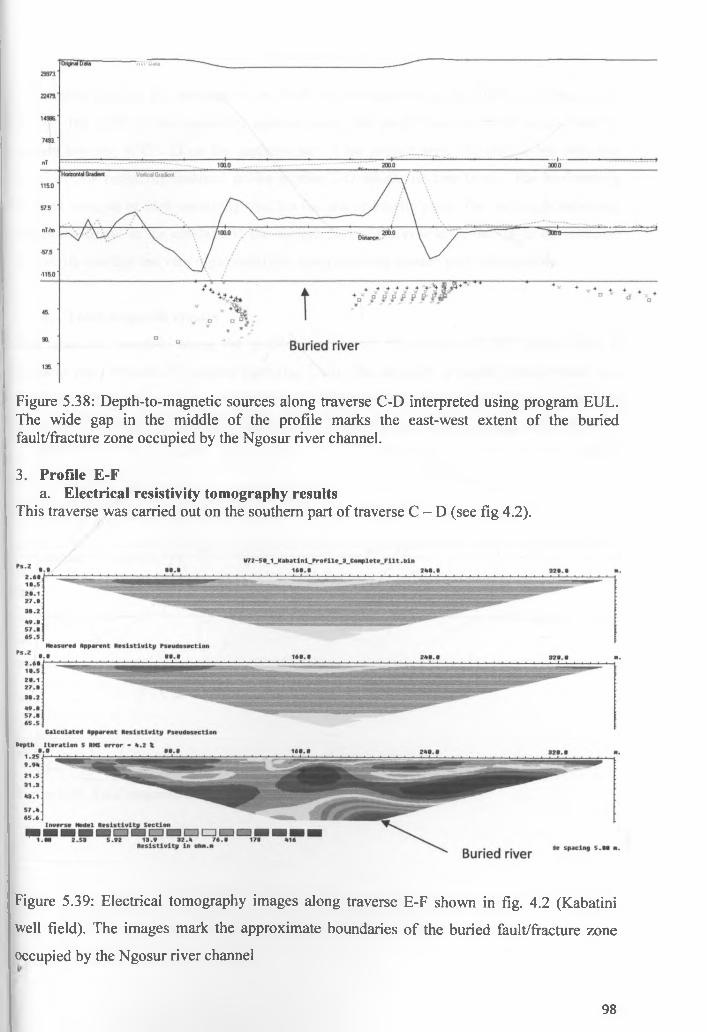
Figure 5.38: Depth-to-magnetic sources along traverse C-D interpreted using program EUL. The wide gap in the middle o f the profile marks the east-west extent o f the buried fault/fracture zone occupied by the Ngosur river channel.
3. Profile E-Fa. Electrical resistivity tomography results
This traverse was carried out on the southern part o f traverse C - D (see fig 4.2).
Figure 5.39: Electrical tomography images along traverse E-F shown in fig. 4.2 (Kabatini
well field). The images mark the approximate boundaries o f the buried fault/fracture zone
occupied by the Ngosur river channel
98

The results indicate the presence o f one level o f low resistivity at the depth o f 60 meters (fig
5.39). The width o f low resistivity material along this profile reduces to 40 meters from 70
meters traverse o f C - D on the northern part o f the project area. The profile has only one
level o f low resistivity material unlike profile C-D which has two levels. The horizontally
layered material o f high resistivity overlies the low resistivity zone. The very high resistivity
zones are found at the central and the eastern part o f the profile. A thin layer o f moderate
resistivity overlies the very high resistivity material on the eastern part o f the profile.
b. Total magnetic results
The magnetic anomaly along the profile is observed 50 meters and 240 meters from E
(eastern part) towards F (western part),(fig 5.40). The anomaly is mostly concentrated at a
shallow depth with two exceptional places at 90 meter and 140 meters from the eastern part
o f the profile. Magnetic anomaly is noted to be deeper than other places along the profile.
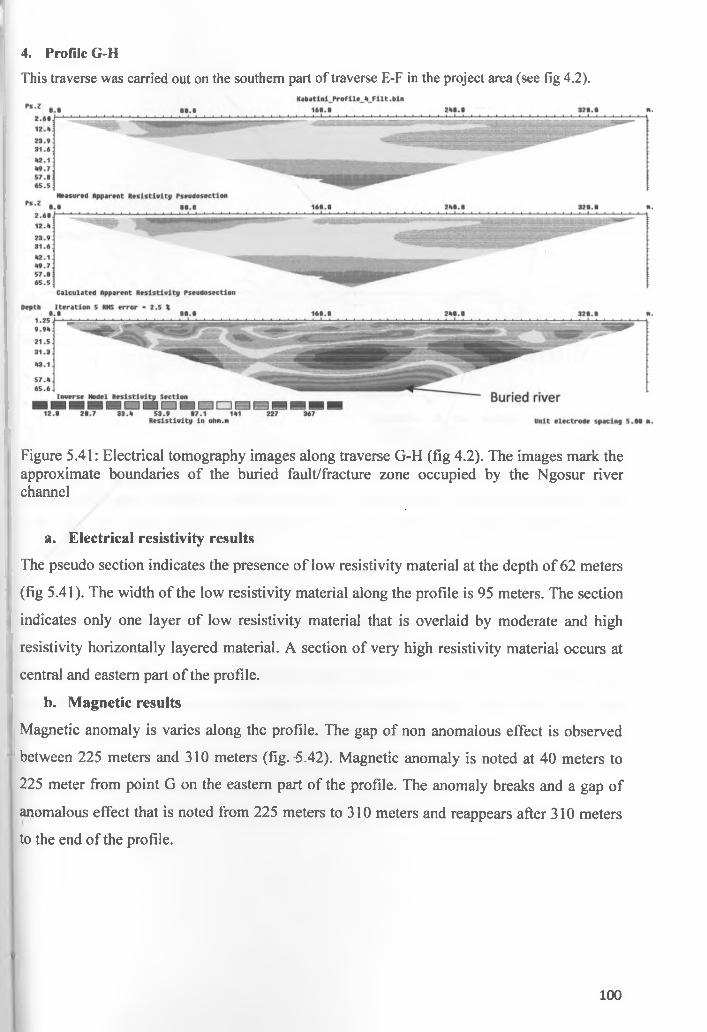
4. Profile G-H
T his traverse w as carried out on the southern part o f traverse E-F in the project area (se e f ig 4 .2 ).
Figure 5.41: Electrical tomography images along traverse G-H (fig 4.2). The images mark the approximate boundaries o f the buried fault/fracture zone occupied by the Ngosur river channel
a. Electrical resistivity results
The pseudo section indicates the presence o f low resistivity material at the depth o f 62 meters
(fig 5.41). The width o f the low resistivity material along the profile is 95 meters. The section
indicates only one layer o f low resistivity material that is overlaid by moderate and high
resistivity horizontally layered material. A section o f very high resistivity material occurs at
central and eastern part o f the profile.
b. Magnetic results
Magnetic anomaly is varies along the profile. The gap o f non anomalous effect is observed
between 225 meters and 310 meters (fig .-5.42). Magnetic anomaly is noted at 40 meters to
225 meter from point G on the eastern part o f the profile. The anomaly breaks and a gap o f
anomalous effect that is noted from 225 meters to 310 meters and reappears after 310 meters
to the end o f the profile.
100

Figure 5.42: D epth-to-m agnetic sources a lon g traverse G -H interpreted using program E U L E R . The/
w id e gap in the m iddle o f the profile marks the east-w est exten t o f the buried fault/fracture zone
occu p ied by the N gosu r river channel.
5.6.4 Total magnetic anomaly distribution in the project area
The magnetic contours o f 29000,29500, 30000,30500,31000 , 31500 and 32000 show
anomalous regions. The high anomalous regions contours are 32500,33000,and 3350.
Contour 31500 occupies awider area on the northern part o f the area, narrows down to center
and widens again at the southern part o f the project area. The low low level contours indicate
the location o f the buried river (fig 6.3).

CHAPTER SIX
6.0 SUMMARY AND CONCLUSION
6.1 Summary
The results o f investigations executed by the electrical resistivity tomography method prove
the existence o f a relationship between the distribution o f electric resistivity and the
geological structure. This relationship is well visible in a geological structure with simple
conditions, especially where soils have contrasting values o f electric resistivity, e. g., sands
and clays or dry and saturated sands. We can see this situation on profiles situated in the
buried river channel o f the Kabatini area. The Electrical resistivity tomography shows clearly
that there exists buried river in Kabatini area. This is shown by the low resistivity levels
noted in profiles A-B, C-D, E-F, and G-H. The river runs from the northern part of the area
traversing all the four profiles. The electrical resistivity tomography shows the existences of
river channels at a depth o f 60 meters in all the four profiles. The other shallow channels are
shown by low resisvitly at 10m - 18 m in all the four profiles. The processed data shows that
the buried river flows from the northern part o f profile A-B to southern part of profile G -N ,
(see fig 6 .1 and 6.2). The width o f the river channel along profiles A - B , C-D, E-F, and G-H
is 100m, 80m, 50m and 100m respectively according to the electrical resistivity tomography
results
I t r r j t l a a •. O f . * r r « r * J . t *
U .l >•./ IM St.9 l / . t tkf Jtl M/•M UtUtly m mkm.m Mill *1m 1>m » I.M m.
Fig 6.1(a)
Fig 6.1(b) Pseudo-sections showing buried river channel occurring at a depth o f 60 m. The
width o f the river is about 100 m as indicated by fig 6 .1a above for profile G - H .
V
102

G
M
Figure 6.2: River Ngosur shown traversing the four profiles (AB, CD, EF, and GH) at a depth o f 60 meters (G - M and H - N) from the surface
The vertical electrical sounding indicates that there is an underground river channel in
Kabatini area. The channel is confined by a layer o f resistivity values varying between low to/
high. The river channel flows in the north - south direction and when it reaches kabatini,
some o f its water disperses into the highly porous material to feed kabatini aquifer. VES
results shows that the entire area covered by vertical electrical sounding (150 m by 150 m)
forms part o f the kabatini aquifer. The aquifer extends outside the study area as noted by the
horizontal Iso- resistivity maps. The average depth o f Kabatini aquifer exceeds 165m as
noted from the 2D vertical sections. The software used was able to analyze the Kabatini
aquifer up to the depth o f 165 m. While it is noted that some water feeds the aquifer, the rest
flows to the south defining a north - south geometrical trend. The trend is noted at depth
levels o f 50m, 75m, 100m, 125m, and 150 m as shown by horizontal Iso-resistivity maps.
The trend of the river is controlled by the fault line running in the north - south direction.
103

The location o f these channels is also recorded by the total magnetic effect survey. The
anomalous effect appears in the four profiles, showing the direction o f the river channel. The
total magnetic map (fig.6.3) shows that the river channel is oriented in the N - S direction.
Location of buried river as shown by magnetic a normally
3 3 5 0 0
3 3 0 0 0
3 2 5 0 0
3 2 0 0 0
3 1 5 0 0
3 1 0 0 0
3 0 5 0 0
3 0 0 0 0
2 9 5 0 0
'2 9 0 0 0
Fig 6.3: The map shows the distribution of the total magnetic anomaly in Kabatini well field. Note the
low total magnetic a normally in middle showing the position of the buried river.
6.2 Concluding remarks
The research did not only pave way for a clear picture o f the hydrogeological knowledge of
Kabatini in other to create awareness on the productive and prolific aquifer for sustainable
groundwater supply but act as guides to both the government and individuals especially those
involved in groundwater development on the areas and depths boreholes could be sited and
drilled for sustainable water supply. It has-been ascertained that Kabatini area has got a river
channel that is oriented N- S geometrically as seen in figures 5.26, 5.27, 5.28, 5.29, and 5.30.
It is also noted that the underground river channel traversing Kabatini area, feeds the kabatini
aquifer as indicated by vertical electrical sounding and electrical resistivity tomography. The
depth o f the river channel and the thickness o f the Kabatini aquifer exceed 165m. The bottom
layers o f stations {(1W, 0), (0, 0), (IE, 0), (2E, 0)}, {(1W, IS), (IE, IS), (2E, IS)}, {(1W, 2S), (IE,
2S), (2E, 2S)},{( 1W, 3S), (0,3S), (IE, 3S), (2E, 3S)}, on fig 4.2a have very low resistivity values
v indicating that the depth o f the aquifer extends beyond these layers (165m). It is also noted
104

that the river channel occurs on the eastern part o f the study area as proved by all the methods
used in this research.
6.3 Recommendation
The following are the recommendations made from this study;
I. Drilling o f the boreholes in Kabatini area should be deeper than 60 m from the surface
since the channels that contain water occur at this depth and extends beyond the depth
o f 165m for the better yield.
II. Future research work should be carried out using Vertical electrical sounding and
other geophysical methods that could cover deeper and a more wide area.
105

References
Abd El-Rahman, A. and Khaled, M.A., 2005: Geophysical Exploration for Groundwater Possibilities in Wadi El-Rahba, Eastern Desert, Egypt, Geophysical Society Journal, 3(1), pp 99-108.Al-Abaseiry, A., Abdel Rahman and Ezz El-Deen, M.M., 2005: Geophysical Exploration for Groundwater Potientialities in Wadi El-Rahba, Eastern Desert, Egypt, Geophysical SocietyJournal, 3(1), pp 119-1128.
Alotaibi, A.M. and AlAmri, A.M., 2007: Ground Water Potentialities o f Wadi Malakan- Southem Makkah AlMokadash City, Saudi Arabia, Geophysical Society Journal, 5(1), pp 101-116.Baker, B.H., Mohr,P.A and Williams, L.A.J., 1972: Geology of the Eastern Rift system of Africa, Geological society o f America, Special paper No. 136
Barongo J., 2007: Mawari Project (unpublished report), University o f Nairobi.
Barritt, S., 1993: The African Magnetic Mapping Project. ITC Journal, 2, pp 122-131.
Becht, R., Fred Mwango, Fred A. Muno., 2005. Groundwater links within Rift Valley Lakes. 11th World Lakes Conference, Nairobi.
Bernard, J. and Valla, P. (1991) Groundwater exploration in fissured media with electric and VLF methods, Geoexploration, No. 27,pp 81-91.Bonini, W. and Hickok, E., 1969: Seismic refraction method in ground-water exploration. Am. Inst. Min., Metallurgy Petr. Eng. Trans., Vol. 211, pp 485-488.
Carmichael, R. and Henry, G. J., 1977: Gravity exploration for groundwater and bedrock topography in glaciated areas. Geophysics, Vol. 42, pp 850-859
Choudhury, K., D.K. Saha and P. Chakraborty, 2001: Geophysical study for saline water intrusion in a coastal alluvial terrain, J. Appl. Geophys., Vol.46, pp 189-200.
Clarke, M., Woodhall, D., Allen, D., and Darling, G., 1990: Geological, volcanological and hydrological controls o f the occurrence o f geothermal activity in the area surrounding Lake Naivasha. Technical report: Government o f Kenya, Ministry o f Energy/British Geological Survey.
Daniels F. and Alberty R.A., 1966: Physical Chemistry. John Wiley and Sons, Inc. deGroot- Hedlin, C. and Constable, S., 1990: Occam's inversion to generate smooth, two dimensional models form magnetotelluric data. Geophysics, No.55, pp 1613-1624
106

de Groot - Hedlin C. and Constable S.C. 1990. Occam’s inversion to generate smooth, two dimensional model from magnetotelluric data. Geophysics 58, pp 1603 - 1628.
Dey, A. and Morrison, H. 1979: Resistivity modeling for arbitrary shaped two dimensional structures. Geophys. Prospect., 27:106-136.
Dey A. and Morrison H.F. 1979a: Resistivity modeling for arbitrary shaped two-dimensional structures. Geophysical Prospecting 27, 1020-1036.
Dey A. and Morrison H.F., 1979b. Resistivity modeling for arbitrarily shaped three dimensional shaped structures. Geophysics 44, 753-780.
Dey, A., and Morrison, H. F, 1979, Resistivity modeling for arbitrarily shaped three- dimensional structures: Geophysics, 44, 753-780.
Electrical imaging surveys for environmental and engineering studies; a practical guide to 2d and 3d surveys, www.geoelectrical.com. Visited on 17/2/2010
Elkheder, H.I., Shereef, M.R., El Galladi, A.A. and Pederson, L.B. 2004 Geoelectric Study on Quaternary Groundwater Aquifers in Northwest Sainai, Egypt, Geophysical Society Journal, 2(1): pp. 69-74.
EL-Waheidi, M.M., F. Merlanti and M. Pavan, 1992: Geoelectrical resistivity survey o f the central part ofAzraq Basin (Jordan) for identifying saltwater/freshwater interface, J. Appl. Geophys., 29, 125-133.Fitterman, D. and Stewart, M. 1986: Transient electromagnetic sounding for groundwater. Geophysics, 51(4):995-1005.
Frohlich, R.K. and W.E. Kelly., 1987: Estimates o f specific yield with the geoelectric resistivity method in glacial aquifers, J. Hydrol., 97, pp. 33-44.
Frohlich, R.K. and D. Urish 2002: The use o f geoelectrics and test wells for the assessment of groundwater quality o f a coastal industrial site, J. Appl. Geophys., 50, pp. 261-278. Geological survey o f Iran.
Griffiths, D. and Baker, R., 1993: Two-dimensional resistivity imaging and modelling in areas o f complex geology. Journal o f Applied Geophysics, 29, pp. 211-226.
Griffiths, D. and Turnbull, J.,1985: A multi-electrode array for resistivity surveying. First Break, 3(7), pp. 16-20.
Haggard, L, Proton\ Precession Ferrous Metal Detector, Practical Electronics, pp. 782-793, October, 1970
V
107

Hosny, M.M., EZZ El-Deen, Abdallah, A.A., Abdel Rahman and Barseim, M.S.M.,2005
Geoelectrical Study on the Groundwater Occurrence in the Area Southwest o f Sidi Barrani, Northwestern Coast, Egypt, Geophysical Society Journal, 3(1), pp 109-118.
Ghosh, D.P., 1971: Inverse filter coefficient for the computation o f apparent resistivity standard curves for a horizontal stratified earth , Geophysical prospecting 19, pp. 769 - 775.
Ibrahim, E.H., Shereef, M.R., El Galladi, A.A. and Pederson, L.B.,2004: Geoelectric Study on Quaternary Groundwater Aquifers in Northwest Sainai, Egypt, Geophysical Society Journal, 2(1), pp. 69-74.
Jackson, P.N., S.D. Taylor and P.N. Stanford 1978: Resistivity- porosity-particle shape relationships for marine sands, Geophysics, 43, pp. 1250-1268.
Kaya, G.K. 2001: Investigation o f groundwater contamination using electric and electromagnetic methods at an open waste-disposal site: a case study from Isparta, Turkey, Environ. Geoi, 40, pp.725-731
Keller G.V. and Frischknecht F.C.,1966: Electrical methods in geophysical prospecting. Pergamon Press Inc., Oxford.
Kelly, E.W. 1976: Geoelectric sounding for delineating ground water contamination, Ground Water, 14, pp.6-11.
Kessels, W., I. Flentge and H. Kolditz 1985: DC geoelectric sounding to determine water content in the salt mine (FRG), Geophys. Prospect., 33, pp.456-446.
Koefoed 0.,1979. Geosounding Principles 1 : Resistivity sounding measurements. Elsevier Science Publishing Company, Amsterdam.
Kossinski, W.K. and W.E. Kelly 1981: Geoelectricsounding for predicting Aquifer Properties, Ground Water, pp. 163-171.
Kuria Z.N, 1999.Hydrogeology o f lake Nakuru drainage basin using GIS data and electrical resistivity, MSc. Thesis, University o f Nairobi.
LaBrecque, D.J., Miletto, M., Daily, W., Ramirez, A. and Owen, E., 1996. The effects o f noise on Occam’s inversion of resistivity tomography data. Geophysics, 61, pp. 538-548.
LaBrecque, D., Morelli, G., Daily, W., Ramirez, A., and Lundegard, P., 1999, Occam’s inversion of 3Delectrical resistivity tomography, in Oristaglio M., and B. Spies, Eds., Three Dimensional Electromagnetics,: Soc. Expl.Geophys.
108

Loke, M. and Barker, R. 1996. Rapid least-squares inversion of apparent resistivity pseudosections by a quasi-newton method. Geophysical Prospecting, 44 , pp. 131-152.
Loke, M.H., Dahlin, T., 1997. A combined Gauss -Newton and quasi-Newton inversion method for the interpretation o f apparent resistivity pseudosections. Procs. 3rd Meeting o f the European Association for Environmental and Engineering Geophysics, 8- 11 Sept. 1997, Aarhus, Denmark, pp. 139- 142.
Loke, M.H., 2000. Topographic modelling in resistivity imaging inversion. 62nd EAGE Conference & Technical Exhibition Extended Abstracts, D-2.
Mathu 2006, Mawari project (unpublished report), University o f Nairobi
Matias, M.J.S. 2002: Squary array anisotropy measurements and resistivity sounding interpretation,./. Appl. Geophys., pp 49. 185-194.
McCall, C.J.H., 1967, Geology o f the Nakuru - Thomson’s falls - lake Hannington area, Report No. 78 . Kenya Geol. Surv., Nairobi, Kenya.
Michel, R., Jean-Claude, P., Diouf, S., Beauvais, A., Dione, F.,and Dione, F. 1999: Electrical imaging o f lateritic weathering mantles over granitic and metamorphic basement of eastern Senegal, West uppercaseAfrica. Journal o f Applied Geophysics, 41, pp. 335-344.
Mousa, D.A. 2003: The role o f 1-D sounding and 2-D resistivity inversions in delineating the near-surface lithologic variations in Tushka area, south o f Egypt, Geophysical Society Journal, 1, pp. 57-64.Nabidi, I. K.2002: Development of 3-D conceptual hydrogeological model for Lake Naivasha area. Msc. Thesis, WREM. Enschede, ITC.
Nigm, A.A., Elterb, R. A., Nasr, F.E. and Thobaity, H.M. 2008 Contribution o f Ground Magnetic and Resistivity Methods in Groundwater Assessment in Wadi Bany Omair. Holy Makkah Area, Saudi Arabia, Egyptian, Geophysical Society Journal, 6(1): 67-79.
Nowroozi, A., Horrocks, B. and Henderson, P., 1999: Saltwater intrusion into the freshwater aquifer in the eastern shore o f Virginia: a reconnaissance electrical resistivity survey, J. Applied Geophysics, 42, pp. 1-22.
OliVar, A., de Lime, L. and Sharma, M.M., 1990: A grain conductivity approach to shaly sandstones. Geophysics, 55, pp. 1347-1356.
Onyere,S.M.,1997, Structural analysis o f the drainage basin o f Kenyan Rift Valley lakes within the Aberdare detachment using satellite data, GIS and field observation, PhD Thesis, Department o f Geology , University o f Nairobi.
*109

Pastor, M. S. 2001. Geophysical study of the groundwater system south o f lake Naivasha, Kenya, International Institute for Aerospace Survey and Earth Sciences, The Netherlands. Res2DINV Manual, 2003. Geotomo Sofware, 5 CangkatMiden Loroung 6 , Miden Heights, 11700 Gelugor, Penang,Malaysia (www.geoeletrical.com)
Serson, P.H., A Simple Proton Precession Magnetometer, Dominion Observatory, Ottawa, Canada, 1962Smith, M. and Mosley, P. 1993, Crustal heterogeneity and basement influence on the development o f the Kenya Rift, East Africa, Tectonics, Vol.12, No.2,pp. 592-606.
Sporry, R. 2001. Lecture material on Resistivity. Earth System Analysis Department, ITC.
Stefanesco, S., C. Schlumberger, and M. Schlumberger. The distribution o f electrical potential about a point electrode in an earth o f horizontal, homogeneous, and isotropic beds. J. Phys. Radium 1, pp. 130-141, 1930.Taylor, K., Widmer, M., and Chesley, M. 1992. Use o f transient electromagnetics to define local hydrogeology in an arid alluvial environment. Geophysics, 57(2), pp. 343-352.Troisi, S., C. Fallicos, S. Straface and E. Migliari 2000: Application o f kriging with external drift to estimate hydraulic conductivity from electrical resistively data in unconsolidated deposits near Montato Uffiigo, Italy, Hydrogeol. J., 8 , pp. 356-367.
Van Overmeeren, R., 1989: Aquifer boundaries explored by geoelectrical measurements in thecoastal plain o f Yemen, A Case o f Equivalence. Geophysics, 54, pp. 38-48.
Vouillamoz, J.M., M. Descloitres, J. Bernard, P. Fourcassier and L. Romagny, 2002: Application of integrated magnetic resonance sounding and resistivity methods for borehole implementation. A case study in Cambodia, J. Appl. Geophysics, 50, pp. 67-81.
Waters, G.S. and Phillips, G., A New Method o f Measuring the Earth's Magnetic Field, Geophys. Prospecting 1-9, 1956 Serson, P.H., U.S. Patent No. 3,070,745, 1962
Whitely R.,1973: “Electrode arrays in Resistivity and induced polarization prospecting a review” Bulleting o f the Australian Society o f Exploration Geophysics, pp. 1-29.
Yadav, G.S. and H. Abolfazli ,1998: Geoelectric soundings and their relationship to hydraulic parameters in semiarid regions o f Jalore, Northwestern India, J. Appl. Geophys., 39, pp. 35- 51.
Yechieli, Y., 2000: Fresh-saline ground water interface in the Western Dead Sea area, Ground Water, 38, pp. 615-623.
, ►
Parasnis, D. 1997 Principle o f Applied Geophysics, London: Chapman & Hall., 275 p.
110

Young, M.E., R.G.M. De Bruijin and A. Salim al-lsmaily, 1998: Report: exploration of an alluvial aquifer in Oman by time-domain electromagnetic sounding, Hydrogeol. j w> 6, pp-
383-393.
Youssef, A.M.A., Abdellatief, T.A., El Mousa, S.E.D. and Tamamy, M.M.A., 2004 Geoelectrical Survey to Delineate the Extension of the Water Bearing Formations in Wadi Gharandal, Southwest Sainai, Egypt, Geophysical Society Journal 2(1), pp.75-84.
Zohdy, A., Eaton, G., and Mabey, D.,1974, Application of surface geophysics to grou ft V)ater investigations,Techniques of Water-Resources Investigation o f the United States G e£,1°8,cal
Survey, Book 2, Dl.,ger and
Zohdy A. A. R„ 1989. A new method for the automatic interpretation of Schlumbe’Wenner sounding curves; Geophysics, Vol. 54, No.2, pp245-253 ^t\0n inZohdy, A.A.R. 1969: Application of deep electrical soundings for groundwater explcr FHawaii, Geophysics, pp.584-600.
Young, M.E., R.G.M. De Bruijin and A. Salim al-lsmaily, 1998: Report: exploration of an alluvial aquifer in Oman by time-domain electromagnetic sounding, Hydrogeol. J., 6, pp. 383-393.
Youssef, A.M.A., Abdellatief, T.A., El Mousa, S.E.D. and Tamamy, M.M.A., 2004 Geoelectrical Survey to Delineate the Extension of the Water Bearing Formations in Wadi Gharandal, Southwest Sainai, Egypt, Geophysical Society Journal, 2(1), pp.75-84.
Zohdy, A., Eaton, G., and Mabey, D.,1974, Application of surface geophysics to groundwater investigations,Techniques of Water-Resources Investigation of the United States Geological Survey, Book 2, Dl.
Zohdy A. A. R., 1989. A new method for the automatic interpretation of Schlumberger and Wenner sounding curves; Geophysics, Vol. 54, No.2, pp245-253Zohdy, A.A.R. 1969: Application of deep electrical soundings for groundwater exploration in Hawaii, Geophysics, pp.584-600.
I l l