geostatistics for gaussian processesgpss.cc/mock09/slides/wackernagel.pdf · geostatistics for...

NIPS 2009 • Whistler, december 2009

IntroductionGeostatistical ModelCovariance structure

CokrigingConclusion

Geostatistics forGaussian processes

Hans Wackernagel

Geostatistics group — MINES ParisTechhttp://hans.wackernagel.free.fr

Kernels for Multiple Outputs and Multi-task LearningNIPS Workshop, Whistler, July 2009

Hans Wackernagel Geostatistics for Gaussian processes

http://hans.wackernagel.free.fr



CokrigingConclusion

Introduction


Geostatistics and Gaussian processes

Geostatisticsis not limited to Gaussian processes,it usually refers to the concept of random functions,it may also build on concepts from random sets theory.

Geostatistics

Geostatistics:is mostly known for the kriging techniques.

Geostatistical simulation of random functions conditionnally ondata is used for non-linear estimation problems.Bayesian inference of geostatistical parameters has become atopic of research.Sequential data assimilation is an extension of geostatisticsusing a mechanistic model to describe the time dynamics.

In this (simple) talk:we will stay with linear (Gaussian) geostatistics,concentrate on kriging in a multi-scale and multi-variate context.

A typical application may be:the response surface estimation problemeventually with several correlated response variables.

Statistical inference of parameters will not be discussed.We rather focus on the interpretation of geostatistical models.

Geostatistics: definition

Geostatistics is an application of the theory of regionalized variablesto the problem of predicting spatial phenomena.

(G. MATHERON, 1970)

We consider the regionalized variable z(x) to bea realization of a random function Z (x).

Stationarity

For the top series:we think of a (2nd order) stationary model

For the bottom series:a mean and a finite variance do not make sense,rather the realization of a non-stationary process without drift.

Second-order stationary modelMean and covariance are translation invariant

The mean of the random function does not depend on x :

E[

Z (x)]

= m

The covariance depends on length and orientation ofthe vector h linking two points x and x′ = x + h:

cov(Z (x), Z (x′)) = C(h) = E[ (

Z (x)−m)·(

Z (x+h)−m) ]

Non-stationary model (without drift)Variance of increments is translation invariant

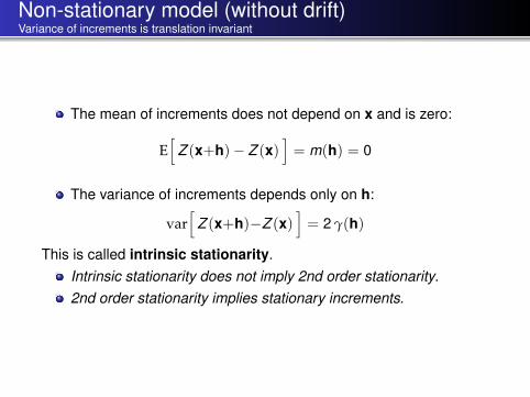
The mean of increments does not depend on x and is zero:

E[

Z (x+h)− Z (x)]

= m(h) = 0

The variance of increments depends only on h:

var[

Z (x+h)−Z (x)]

= 2 γ(h)

This is called intrinsic stationarity.Intrinsic stationarity does not imply 2nd order stationarity.2nd order stationarity implies stationary increments.

The variogram

With intrinsic stationarity:

γ(h) =12

E[ (

Z (x+h)− Z (x))2 ]

Properties- zero at the origin γ(0) = 0- positive values γ(h) ≥ 0- even function γ(h) = γ(−h)

The covariance function is bounded by the variance:C(0) = σ2 ≥ |C(h) |The variogram is not bounded.A variogram can always be constructedfrom a given covariance function: γ(h) = C(0)−C(h)The converse is not true.

What is a variogram ?

A covariance function is a positive definite function.

What is a variogram?A variogram is a conditionnally negative definite function.In particular:

any variogram matrix Γ = [γ(xα−xβ)] isconditionally negative semi-definite,

[wα]>[γ(xα−xβ)

][wα] = w>Γ w ≤ 0

for any set of weights with

n

∑α=0

wα = 0.

Ordinary kriging

Estimator: Z ?(x0) =n

∑α=1

wα Z (xα) withn

∑α=1

wα = 1

Solving:

arg minw1,...,wn,µ

[var (Z ?(x0)− Z (x0))− 2µ(

n

∑α=1

wα − 1)

]yields the system:

n

∑β=1

wβ γ(xα−xβ) + µ = γ(xα−x0) ∀α

n

∑β=1

wβ = 1

and the kriging variance: σ2K = µ +

n

∑α=1

wα γ(xα−x0)



CokrigingConclusion

Anisotropy of the random functionConsequences in terms of sampling design

Mobile phone exposure ofchildren

by Liudmila Kudryavtseva


http://perso.rd.francetelecom.fr/joe.wiart/

Phone position and child headHead of 12 year old child

SAR exposure (simulated)

Max SAR for different positions of phoneThe phone positions are characterized by two angles

The SAR values are normalized with respect to 1 W.Regular sampling.

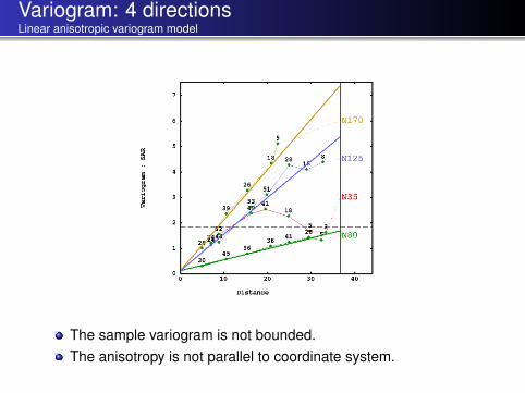
Variogram: 4 directionsLinear anisotropic variogram model

The sample variogram is not bounded.The anisotropy is not parallel to coordinate system.

Max SAR kriged map

Prediction errorKriging standard deviations σK

The sampling design is not appropriate due to the anisotropy.

Prediction errorDifferent sample design

Changing the sampling design leads to smaller σK.



CokrigingConclusion

Geostatistical Model




CokrigingConclusion

Linear model of coregionalization

The linear model of coregionalization (LMC) combines:a linear model for different scales of the spatial variation,a linear model for components of the multivariate variation.


Two linear models

Linear Model of Regionalization: Z (x) =S∑

u=0Yu(x)

E[

Yu(x+h)− Yu(x)]

= 0

E[ (

Yu(x+h)− Yu(x))·(

Yv (x+h)− Yv (x)) ]

= gu(h) δuv

Linear Model of PCA: Zi =N∑

p=1aip Yp

E[

Yp

]= 0

cov(

Yp, Yq

)= 0 for p 6= q

Linear Model of Coregionalization

Spatial and multivariate representation of Zi (x) usinguncorrelated factors Y p

u (x) with coefficients auip:

Zi (x) =S

∑u=0

N

∑p=1

auip Y p

u (x)

Given u, all factors Y pu (x) have the same variogram gu(h).

This implies a multivariate nested variogram:

Γ(h) =S

∑u=0

Bu gu(h)

Coregionalization matrices

The coregionalization matrices Bu characterizethe correlation between the variables Ziat different spatial scales.

In practice:1 A multivariate nested variogram model is fitted.2 Each matrix is then decomposed using a PCA:

Bu =[

buij

]=[ N

∑p=1

auip au

jp

]yielding the coefficients of the LMC.

LMC: intrinsic correlation

When all coregionalization matrices are proportional to a matrix B:

Bu = au B

we have an intrinsically correlated LMC:

Γ(h) = BS

∑u=0

au gu(h) = B γ(h)

In practice, with intrinsic correlation, the eigenanalysis of the differentBu will yield:

different sets of eigenvalues,but identical sets of eigenvectors.

Regionalized Multivariate Data Analysis

With intrinsic correlation:

The factors are autokrigeable,i.e. the factors can be computedfrom a classical MDA onthe variance-covariance matrix V ∼= Band are kriged subsequently.

With spatial-scale dependent correlation:

The factors are defined on the basis ofthe coregionalization matrices Buand are cokriged subsequently.

Need for a regionalized multivariate data analysis!

Regionalized PCA ?

Variables Zi (x)

↓Intrinsic Correlation ? no−→ γij (h) = ∑

uBu gu(h)

↓ yes ↓

PCA on B PCA on Bu

↓ ↓Transform into Y Cokrige Y ?

u0p0(x)

↓ ↓

Krige Y ?p0

(x) −→ Map of PC



CokrigingConclusion

Multivariate Geostatistical filtering

Sea Surface Temperature (SST)in the Golfe du Lion


Modeling of spatial variabilityas the sum of a small-scale and a large-scale process

SST on 7 june 2005The variogram of the Nar16 im-age is fitted with a short- and along-range structure (with geo-metrical anisotropy).

Variogram of SST

The small-scale componentsof the NAR16 image

andof corresponding MARS ocean-model output

are extracted by geostatistical filtering.

Geostatistical filteringSmall scale (top) and large scale (bottom) features

3˚

3˚

4˚

4˚

5˚

5˚

6˚

6˚

7˚

7˚

43˚ 43˚

3˚

3˚

4˚

4˚

5˚

5˚

6˚

6˚

7˚

7˚

43˚ 43˚

−0.5 0.0 0.5

3˚

3˚

4˚

4˚

5˚

5˚

6˚

6˚

7˚

7˚

43˚ 43˚

3˚

3˚

4˚

4˚

5˚

5˚

6˚

6˚

7˚

7˚

43˚ 43˚

−0.5 0.0 0.5

NAR16 image MARS model output

3˚

3˚

4˚

4˚

5˚

5˚

6˚

6˚

7˚

7˚

43˚ 43˚

3˚

3˚

4˚

4˚

5˚

5˚

6˚

6˚

7˚

7˚

43˚ 43˚

15 20

3˚

3˚

4˚

4˚

5˚

5˚

6˚

6˚

7˚

7˚

43˚ 43˚

3˚

3˚

4˚

4˚

5˚

5˚

6˚

6˚

7˚

7˚

43˚ 43˚

15 20

Zoom into NE corner

Bathymetry

3˚

3˚

4˚

4˚

5˚

5˚

6˚

6˚

7˚

7˚

43˚ 43˚100

100

200

200200

300

300 300

400

400400

500

500500

600

600600

700

700

700

800

800

800

900

900

900

1000

1000

1000

1100

1100

1200

1200

1300

1300

1400

1400

1500

1500

1600

1600

1700

1700

1800

1800

1900

1900

2000

200021002200 2300 2400

3˚

3˚

4˚

4˚

5˚

5˚

6˚

6˚

7˚

7˚

43˚ 43˚

0 500 1000 1500 2000 2500

Depth selection,scatter diagram

Direct and crossvariogramsin NE corner

Cokriging in NE cornerSmall-scale (top) and large-scale (bottom) components

6˚18'

6˚18'

6˚24'

6˚24'

6˚30'

6˚30'

6˚36'

6˚36'

6˚42'

6˚42'

6˚48'

6˚48'

6˚54'

6˚54'

42˚54'

43˚00'

43˚06'

43˚12'

43˚18'

43˚24'

43˚30'

6˚18'

6˚18'

6˚24'

6˚24'

6˚30'

6˚30'

6˚36'

6˚36'

6˚42'

6˚42'

6˚48'

6˚48'

6˚54'

6˚54'

42˚54'

43˚00'

43˚06'

43˚12'

43˚18'

43˚24'

43˚30'

−0.3 −0.2 −0.1 0.0 0.1 0.2 0.3

6˚18'

6˚18'

6˚24'

6˚24'

6˚30'

6˚30'

6˚36'

6˚36'

6˚42'

6˚42'

6˚48'

6˚48'

6˚54'

6˚54'

42˚54'

43˚00'

43˚06'

43˚12'

43˚18'

43˚24'

43˚30'

6˚18'

6˚18'

6˚24'

6˚24'

6˚30'

6˚30'

6˚36'

6˚36'

6˚42'

6˚42'

6˚48'

6˚48'

6˚54'

6˚54'

42˚54'

43˚00'

43˚06'

43˚12'

43˚18'

43˚24'

43˚30'

−0.3 −0.2 −0.1 0.0 0.1 0.2 0.3

NAR16 image MARS model output

6˚18'

6˚18'

6˚24'

6˚24'

6˚30'

6˚30'

6˚36'

6˚36'

6˚42'

6˚42'

6˚48'

6˚48'

6˚54'

6˚54'

42˚54'

43˚00'

43˚06'

43˚12'

43˚18'

43˚24'

43˚30'

6˚18'

6˚18'

6˚24'

6˚24'

6˚30'

6˚30'

6˚36'

6˚36'

6˚42'

6˚42'

6˚48'

6˚48'

6˚54'

6˚54'

42˚54'

43˚00'

43˚06'

43˚12'

43˚18'

43˚24'

43˚30'

19.0 19.5 20.0 20.5 21.0 21.5 22.0

6˚18'

6˚18'

6˚24'

6˚24'

6˚30'

6˚30'

6˚36'

6˚36'

6˚42'

6˚42'

6˚48'

6˚48'

6˚54'

6˚54'

42˚54'

43˚00'

43˚06'

43˚12'

43˚18'

43˚24'

43˚30'

6˚18'

6˚18'

6˚24'

6˚24'

6˚30'

6˚30'

6˚36'

6˚36'

6˚42'

6˚42'

6˚48'

6˚48'

6˚54'

6˚54'

42˚54'

43˚00'

43˚06'

43˚12'

43˚18'

43˚24'

43˚30'

19.0 19.5 20.0 20.5 21.0 21.5 22.0

Different correlation at small- and large-scale .

Consequence

To correct for the discrepancies between remotely sensed SST andMARS ocean model SST, the latter was thoroughly revised in orderbetter reproduce the path of the Ligurian current.



CokrigingConclusion

Covariance structure


Separable multivariate and spatial correlationIntrinsic correlation model (Matheron, 1965)

A simple model for the matrix Γ(h)of direct and cross variograms γij (h) is:

Γ(h) =[

γij (h)]

= B γ(h)

where B is a positive semi-definite matrix.

The multivariate and spatial correlation factorize (separability).

In this model all variograms are proportionalto a basic variogram γ(h):

γij (h) = bij γ(h)

Codispersion CoefficientsMatheron (1965)

A coregionalization is intrinsically correlatedwhen the codispersion coefficients:

ccij (h) =γij (h)√

γii (h) γjj (h)

are constant, i.e. do not depend on spatial scale.With the intrinsic correlation model:

ccij (h) =bij γ(h)√bii bjj γ(h)

= rij

the correlation rij between variables isnot a function of h.

Intrinsic Correlation: Covariance Model

For a covariance function matrix the model becomes:

C(h) = V ρ(h)

whereV =

[σij

]is the variance-covariance matrix,

ρ(h) is an autocorrelation function.

The correlations between variables do not depend on the spatialscale h, hence the adjective intrinsic.

Testing for Intrinsic CorrelationExploratory test

1 Compute principal components for the variable set.2 Compute the cross-variograms between principal components.

In case of intrinsic correlation, the cross-variogramsbetween principal components should all be zero.

Cross variogram: two principal components

�

��

��

��

��

��

��

The ordinate is scaled using the perfect correlation envelope(Wackernagel, 2003)The intrinsic correlation model is not adequate!

Testing for Intrinsic CorrelationHypothesis testing

A testing methodology based on asymptotic joint normality of thesample space-time cross-covariance estimators is proposed inLI, GENTON and SHERMAN (2008).



CokrigingConclusion

Cokriging


Ordinary cokriging

Estimator: Z ?i0,OK(x0) =

N

∑i=1

ni

∑α=1

w iα Zi (xα)

with constrained weights: ∑α

w iα = δi,i0

A priori a (very) large linear system:N · n + N equations,(N · n + N)2 dimensional matrix to invert.

The good news:for some covariance modelsa number of equations may be left out— knowing that the corresponding w i

α = 0.

Data configuration and neighborhood

Data configuration: the sites of the different types of inputs.

Are sites shared by different inputs — or not?

Neighborhood: a subset of the available data used in cokriging.

How should the cokriging neighborhood be defined?What are the links with the covariance structure?

Depending on the multivariate covariance structure,data at specific sites of the primary or secondary variablesmay be weighted with zeroes— being thus uninformative.

Data configurationsIso- and heterotopic

primary data secondary data

Heterotopic data

Sample sites

may be different

covers whole domain

Sample sites

are sharedIsotopic data

Secondary data

Dense auxiliary data

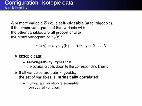
Configuration: isotopic dataAuto-krigeability

A primary variable Z1(x) is self-krigeable (auto-krigeable),if the cross-variograms of that variable withthe other variables are all proportional tothe direct variogram of Z1(x):

γ1j (h) = a1j γ11(h) for j = 2, . . . , N

Isotopic data:self-krigeability implies thatthe cokriging boils down to the corresponding kriging.

If all variables are auto-krigeable,the set of variables is intrinsically correlated:

multivariate variation is separablefrom spatial variation.

Configuration: dense auxiliary dataPossible neighborhoods

H H

primary data H target point secondary data

HA

CB

D H

Choices of neighborhood:A all dataB multi-collocated with target and primary dataC collocated with targetD dislocated

Neighborhood: all data

H

primary data

target point

secondary data

H

Very dense auxiliary data (e.g. remote sensing):large cokriging system, potential numerical instabilities.

Ways out:moving neighborhood,multi-collocated neighborhood,sparser cokriging matrix: covariance tapering.

Neighborhood: multi-collocated

H

H

primary data

target point

secondary data

Multi-collocated cokriging can be equivalent to full cokrigingwhen there is proportionality in the covariance structure,for different forms of cokriging: simple, ordinary, universal

Neighborhood: multi-collocatedExample of proportionality in the covariance model

Cokriging with all data is equivalent to cokriging with amulti-collocated neighborhood for a model with acovariance structure is of the type:

C11(h) = p2 C(h) + C1(h)C22(h) = C(h)C12(h) = p C(h)

where p is a proportionality coefficient.

Cokriging neighborhoods

RIVOIRARD (2004), SUBRAMANYAM AND PANDALAI (2008) looked atvarious examples of this kind,

examining bi- and multi-variate coregionalization modelsin connection with different data configurations

to determine the neighborhoods resulting fromdifferent choices of models.

Among them:the dislocated neighborhood:

H

primary data

target point

secondary data

H



CokrigingConclusion

Conclusion


Conclusion

Multi-output cokriging problems are very large.Analysis of the multivariate covariance structure may revealthe possibility of simplifying the cokriging system,allowing a reduction of the size of the neighborhood.Analysis of directional variograms may reveal anisotropies(not necessarily parallel to the coordinate system).Sampling design can be improved by knowledge of spatialstructure.

Acknowledgements

This work was partly funded by the PRECOC project (2006-2008)of the Franco-Norwegian Foundation(Agence Nationale de la Recherche, Research Council of Norway)as well as by the EU FP7 MOBI-Kids project (2009-2012).

References

BANERJEE, S., CARLIN, B., AND GELFAND, A.Hierarchical Modelling and Analysis for spatial Data.Chapman and Hall, Boca Raton, 2004.

BERTINO, L., EVENSEN, G., AND WACKERNAGEL, H.Sequential data assimilation techniques in oceanography.International Statistical Review 71 (2003), 223–241.

CHILÈS, J., AND DELFINER, P.Geostatistics: Modeling Spatial Uncertainty.Wiley, New York, 1999.

LANTUÉJOUL, C.Geostatistical Simulation: Models and Algorithms.Springer-Verlag, Berlin, 2002.

LI, B., GENTON, M. G., AND SHERMAN, M.Testing the covariance structure of multivariate random fields.Biometrika 95 (2008), 813–829.

MATHERON, G.Les Variables Régionalisées et leur Estimation.Masson, Paris, 1965.

RIVOIRARD, J.On some simplifications of cokriging neighborhood.Mathematical Geology 36 (2004), 899–915.

STEIN, M. L.Interpolation of Spatial Data: Some Theory for Kriging.Springer-Verlag, New York, 1999.

SUBRAMANYAM, A., AND PANDALAI, H. S.Data configurations and the cokriging system: simplification by screen effects.Mathematical Geosciences 40 (2008), 435–443.

WACKERNAGEL, H.Multivariate Geostatistics: an Introduction with Applications, 3rd ed.Springer-Verlag, Berlin, 2003.

APPENDIX

Geostatistical simulation

Conditional Gaussian simulationComparison with kriging

Simulation (left) Samples (right)

Simple kriging (left) Conditional simulation (right)

See LANTUÉJOUL (2002), CHILÈS & DELFINER (1999)

Geostatisticians do not usethe Gaussian covariance function

Stable covariance functions

The stable1 family of covariances functions is defined as:

C(h) = b exp(−|h|

p

a

)with 0 < p ≤ 2

and the Gaussian covariance function is the case p = 2:

C(h) = b exp

(−|h|

2

a

)

where b is the value at the origin and a is the range parameter.

1Named after the stable distribution function.

Davis data set

The data set from DAVIS (1973) is sampled from a smooth surfaceand was used by numerous authors.

Applying ordinary kriging using a unique neighborhood and astable covariance function with p = 1.5 provides a map of thesurface of the same kind that is obtained with other models, e.g.with a spherical covariance using a range parameter of 100ft.If a Gaussian covariance is used, dramatic extrapolation effectscan be observed, while the kriging standard deviation isextremely low.

Example from Wackernagel (2003), p55 and pp 116–118.

Stable covariance function (p=1.5)Neighborhood: all data

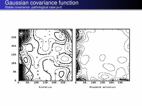
Gaussian covariance functionStable covariance: pathological case p=2

Conclusion

Use of the Gaussian covariance function,when no nugget-effect is added,may lead to undesirable extrapolation effects.Alternate models with the same shape:

the cubic covariance function,stable covariance with 1 < p < 2.

The case p = 2 of a stable covariance function(Gaussian covariance function) is pathological,because realizations of the corresponding random functionare infinitely often differentiable(they are analytic functions):this is contradictory with their randomness(see MATHERON 1972, C-53, p73-74 )2.See also discussion in STEIN (1999).

2Available online at: http://cg.ensmp.fr/bibliotheque/public

http://cg.ensmp.fr/bibliotheque/public

geostatistics for gaussian processesgpss.cc/mock09/slides/wackernagel.pdf · geostatistics for...

Documents