Getting More from Less: Understanding Airline Pricing

John Lazarev∗

Department of EconomicsNew York University

September 23, 2012

Abstract

Motivated by pricing practices in the airline industry, the paper studies the incentives ofplayers to publicly and independently limit the sets of actions they can play later in a game. Ifind that to benefit from self-restraint, players have to exclude all actions that create temptationsto deviate and keep some actions that can deter deviations of others. I develop a set of conditionsunder which these strategies form a subgame perfect equilibrium and show that in a Bertrandoligopoly, firms can mutually gain from self-restraint, while in a Cournot oligopoly they cannot.

∗This paper is a revised chapter of my Stanford Ph.D. dissertation. I thank Peter Reiss and Andy Skrzypacz fortheir invaluable guidance and advice. I am grateful to Lanier Benkard, Jeremy Bulow, Alex Frankel, Ben Golub,Michael Harrison, Jon Levin, Trevor Martin, Michael Ostrovsky, Bob Wilson and participants of the Stanford Struc-tural IO lunch seminar for helpful comments and discussions. All remaining errors are my own. Correspondence:jlazarev@nyu.edu

1

1 Introduction

It is well known that pricing in the airline industry is complex. What is less known is that at

any given moment, the price of a flight ticket is determined by the decisions of not one but two

airline departments: the pricing department and the revenue management department. The pricing

department sets a menu of fares well in advance of the actual flight. This menu is subsequently

updated very rarely. The revenue management department treats the menu as given but decides

in each moment of time which part of the menu to make available for purchase and which to keep

closed. The revenue management department cannot add new fares or change the prices of the

existing ones. As a result, the price of a ticket for a given flight can take only a limited number

of values, not more than the number of fares in the menu. Why would airlines introduce such

a complex structure, in which they effectively restrict their flexibility in changing the prices over

time? At first thought it might seem they can do better by just changing the price over time

without precommitting to a set of fares. One answer may be that, as long as the fare grid is fine

enough, airlines do not lose much from significantly restricting the set of possible prices. This

paper offers an alternative explanation. It demonstrates that, in a strategic environment, firms can

benefit from restricting the set of available actions as long as they can credibly commit to doing

so. Creating a separate department that restricts the set of prices by choosing a menu of fares may

be a way to establish and maintain the credibility of such a commitment.

The idea that the ability to commit to a specific action can be beneficial for an agent is a classic

observation of game theory (Schelling, 1960). The contribution of this paper is to show that in a

broader set of situations, agents can benefit if they can commit to a menu of actions.

As a simple theoretical example of why menus may be desirable, consider a Bertand game

between two firms that sell identical products. The costs of production are zero. The firm that

charges the lower price gets the market demand. If the prices are the same, the market demand

is evenly divided between the firms. In this example, the equilibrium payoffs are zero. Moreover,

the unilateral ability to commit cannot increase the profit of an individual firm. If it commits to a

price other than zero, the competitor can steal the market by charging a slightly lower price and

getting the entire market.

Consider now the following modification. The game consists of two stages: the commitment

stage and the action stage. At the commitment stage, firms can simultaneously and independently

decide to constrain themselves to a menu of prices. Their choices are then publicly observed. Then,

at the action stage, firms independently and simultaneously choose prices from their menus. A

price outside the restricted menu cannot be chosen by firms. The profits are determined according

to the Bertrand game described above.

Unlike in the original game, the equilibrium payoffs in this modification can be positive. More-

over, there exists a subgame perfect equilibrium in which each firm gets a half of the monopoly

profit. The following pair of symmetric strategies form such an equilibrium. At the commitment

stage, each firm chooses a menu that consists of two prices, the monopoly price and zero. If both

firms chose these menus, then charging the monopoly price is an equilibrium in the action stage.

2

Indeed, the only deviation at the action stage is charging zero, which reduces the profit from the

half of the monopoly profit to zero. There are many deviations at the commitment stage but to be

profitable they have to include a price that is higher than zero and less than the monopoly price. If

a firm attempts such deviation, then the competitor will be indifferent between charging zero or the

monopoly price at the action stage. If it charges zero, then the deviator will end up receiving zero.

Thus, deviations at the commitment stage cannot be profitable either. To summarize, Bertrand

competitors can still achieve the monopoly outcome without signing an enforceable contract or

using repeated interactions to enforce monopoly pricing. What they need to do is to exclude a

set of profitable deviations from the monopoly outcome (”temptations”) and keep ”punishment”

actions in case their competitors misbehave at the commitment stage.

This example is in a certain sense limited. Even when a firm undercuts by a very small amount,

the profit of its competitor decreases to zero. This discontinuity of the payoffs guarantees that the

punishment by zero price is a credible threat. If the competitors deviate even by a small amount,

the profit of the opponent drops to zero. For continuous payoffs, these pair of strategies would

not be equilibrium anymore. This paper focuses on a class of games with continuous payoffs and

characterizes pure-strategy subgame-perfect Nash equilibria of a game that has two stages described

above.

This possibility of achieving superior outcomes relies on several assumptions. First, the agents

are free to choose any subsets of the unrestricted action spaces. In particular, these subsets can

be non-convex (for example, include isolated actions). Non-convex subsets, as we will see later,

allow players to achieve payoffs that dominate Nash equilibrium ones. Second, it is important that

the players are able to commit not to play actions outside of the chosen subsets. Without such

commitment, the initial stage will not change the incentives of the players. Finally, the chosen

restricted sets must become public knowledge.

Pricing in the airline industry has all these three components. Airline fares are discrete, with

a small number of fares and significant price gaps. The separation of the two departments creates

some commitment power. Indeed, according to industry insiders, these departments do not actively

interact with each other. Next, the information about fares becomes public immediately through a

company (ATPCO) that collects fares from all pricing departments and distributes them four times

a day to all airlines, travel agents, and reservation systems. This company is jointly owned by 16

major airlines. Therefore, all necessary features implied by the commitment concept are present in

the pricing competition among U.S. airlines.

The paper has three main results. The first result shows that to support other than the Nash

equilibrium outcomes of a one-stage game, players have to constrain their action spaces. Moreover,

at least one player has to choose a subset with more than one action at the commitment stage.

The second result provides a necessary and sufficient condition for an outcome to be supported

by a commitment equilibrium. An important corollary from this result shows that in a Bertrand

oligopoly firms may mutually gain from self-restraint while in Cournot they cannot. For super-

modular games, the third result demonstrates that there is a whole set of outcomes that can be

3

supported by an equilibrium of the two-stage model. This set includes Pareto-efficient outcomes.

The proof of the third result is constructive.

An episode from the history of U.S. airline pricing confirms the theoretical predictions of the

model, namely the first result of the paper. In April 1992, American Airlines tried to abandon the

two department system. They thought that fares were too complex, so the idea was to have only one

fare available at any time. In terms of the model, they tried to commit to a set that included only

one action. Within a week, most major carriers (United, Delta, Continental, Northwest) adopted

the same pricing structure. However, in a week, the airlines started a fare war. That is exactly

what the model predicts: if players do not include any punishment actions, a Bertrand-type price

war (the unique static Nash equilibrium) is the only subgame equilibrium outcome. By November

1992, American Airlines acknowledged that the plan had clearly failed and decided to come back

to setting and manipulating thousands of fares throughout the system (for details see American

Airlines Value Pricing (1992)).

The rest of the paper is organized as follows. Section 2 reviews related literatures. Section 3

presents notation and definitions, and shows that the two-stage modification is a coarsening concept

and can have as an equilibrium both Pareto better and Pareto worse outcomes compared to the

Nash equilibrium outcome. In Section 4, I show that supermodular games is a natural class in

which we can study the two-stage modification as it is the class in which a (pure-strategy) subgame

perfect equilibrium is guaranteed to exist. Section 5 shows that there is a nontrivial set of outcomes

that can be supported as an equilibrium in the two-stage game. Section 6 concludes.

2 Related Literature

This paper contributes to several literatures. First, the paper extends our understanding of the

role of commitment in strategic interactions originally developed by Schelling (1960). In his work,

Schelling gives examples of how a player may benefit from reducing her flexibility. In these examples,

a player receives a strategic advantage by moving first and committing to a particular action. No

matter what the other players do, she will not play a different action. In contrast, in this paper,

the players move simultaneously. As a result, they must recognize that they need some flexibility in

their actions in case other players do not restrict their actions or otherwise deviate. For example,

if a player commits to a single action, then she will have no punishment should other players

deviate. When a player commits to a subset of actions, then her punishment action may differ

from her reward action. Moreover, the punishment may depend on the exact deviation chosen by

an opponent.

Ideally, players would like to sign an enforceable contract that specifies what action each agent

will play. Of course, it may be hard to specify exactly what action each agent should play. Hart

and Moore (2004) recognize this fact and view a contract as a mutual commitment not to play

outcomes that are ruled out by the signed contract. Bernheim and Whinston (1998) show that

optimal contracts, in fact, have to be incomplete and include more than one observable outcome if

4

some aspects of performance cannot be verified. Both papers view contracts as a means to constrain

mutually the set of available actions. This paper assumes that players cannot sign such contracts.

If they choose to restrict their set of available actions, they can only do it independently of each

other.

Thus, this paper is more similar in the spirit to the literature on tacit collusion. It is well known

that if players interact with each other during several periods, they can achieve a certain level of

cooperation even if they act independently of each other. In finite-horizon games, deviations can be

deterred by a threat to switch to a worse equilibrium in later periods (Benoit and Krishna, 1985).

Similarly, in infinite-horizon games, players can use a significantly lower continuation value as a

punishment that supports an equilibrium in the subgame induced by a deviation. This result, known

as the Folk theorem, states that if players are patient enough any individually rational outcome can

be supported by a subgame perfect Nash equilibrium. In contrast, this paper assumes that the game

is played only once. As a result, players cannot use future outcomes to punish deviations. Instead,

they strategically choose a subset of actions that must include credible punishments sufficient to

deter deviations from the proposed equilibrium. These punishments must be executed immediately

to affect any cooperation.

Fershtman and Judd (1987) and Fershtman et al. (1991) studied delegation games in which

players can modify their payoff functions by signing contracts with agents who act on their behalf.

By doing so, the players can change their best responses and therefore play other than a Nash

equilibrium strategy, which may result in achieving a Pareto efficient outcome. This study takes

a different approach. Instead of modifying their payoff functions, players can modify their action

sets in a very specific way. They can exclude a subset of actions but cannot include anything else.

Thus, the model of this paper may be viewed as a specific case of payoff modification: the players

can assign a large negative value to a subset of actions but cannot modify the payoffs in any other

way.

The closest papers to this paper are Bade et al. (2009) and Renou (2009). They develop a

similar two-stage construction in which commitment stage is followed by a one-shot game. The

constructions of their paper, however, are different in several important aspects. In the first paper,

players can only commit to a convex subset of actions. This paper, however, allows players to

choose any subset of actions. If players can choose only a convex subset of actions, then they often

cannot get rid of temptations and keep actions that can be used as punishments, which are key to

the results of this paper.

There are a number of papers that endogenize players’ commitment opportunities.1 This paper

does not address this question. The ability of firms to voluntarily restrict their action space is

assumed. This assumption, however, is motivated by real world practices used by firms in an

important industry: airlines.

1See Rosenthal (1991), Van Damme and Hurkens (1996), and Caruana and Einav (2008), among others.

5

3 Elements of a commitment equilibrium

3.1 Definitions

The game G Economic agents play a one-shot normal-form game, G. The game has three

elements: a set of players I = {1, 2, ..., n}, a collection of action spaces {Ai}i∈I , and a collection of

payoff functions {πi : A1 ×A2 × ...×An −→ R}i∈I . Thus, G = (I,A, π) , where A = A1 × A2 ×... × An and π = π1 × π2 × ... × πn. (In general, the omission of a subscript indicates the cross

product over all players. Subscript −i denotes the cross product over all players excluding i). The

agents make decisions simultaneously and independently, which determines their payoffs. I refer to

a ∈ A as an outcome of G and to π (a) ∈ Rn as a payoff of G.

I assume that for every player i: a) Ai is a compact subset of R, and b) πi is upper semi-

continuous in ai, a−i.

An outcome a∗ ∈ A is called a Nash equilibrium (NE) outcome if there exists a pure-strategy

Nash equilibrium that supports a∗ ∈ A. In other words, a∗ ∈ A is a NE outcome if and only if for

all i ∈ I the following inequality holds:

πi(a∗i , a

∗−i)≥ πi

(ai, a

∗−i)

for any ai ∈ Ai.

Denote the set of all NE outcomes by EG and the set of corresponding NE payoffs by ΠG.

The two-stage game C (G) Consider the following modification of game G. Define C (G) as

the following two-stage game:

Stage 0 (commitment stage). Each agent i ∈ I simultaneously and independently chooses

a non-empty compact subset Ai of her action space Ai. Once chosen, the subsets are publicly

observed.

Stage 1 (action stage). The agents play game GC = (I, A, π) where A = A1 × A2 × ... × An.

In other words, the players can choose actions that only belong to the subsets chosen at stage 0.

The actions outside the chosen subsets Ai can not be played.

In this paper, I study pure-strategy subgame perfect Nash equilibria of C (G).

A strategy for player i in the game C (G) is a set Ai and a function σi which selects, for any

subsets of actions chosen by players other than i, an element of Ai, i.e. σi : A−i −→ Ai. A

pure-strategy subgame perfect Nash equilibrium of C (G) is called an independent simultaneous

self-restraint (commitment) equilibrium of the game G. Formally, a commitment equilibrium is an

n-tuple of strategies, (A∗, σ∗), such that

(i) for all i and any set of actions Ai ∈ Ai,

πi (a∗) ≥ πi(σ∗1, ..., σ

∗i−1, ai, σ

∗i+1, ..., σ

∗n

)for any ai ∈ Ai,

where σ∗j = σ∗j

(A∗−j

)and A∗−j = A∗1 × ...A∗j−1 ×A∗j+1 × ...A∗i−1 × Ai ×A∗i+1...×A∗n;

6

(ii) for all i and any Ai, there exists ai ∈ Ai, such that(ai, σ

∗−i)

is a pure strategy Nash

equilibrium of game G =(I, A∗1 × ...A∗i−1 × Ai ×A∗i+1...×A∗n, π

).

An outcome a∗ ∈ A is called a commitment equilibrium outcome if there exists a commitment

equilibrium that supports a∗ ∈ A, i.e. a∗ =(σ∗1(A∗−1

), ..., σ∗n

(A∗−n

)). Denote the set of all

commitment equilibrium outcomes by EC and the set of corresponding commitment equilibrium

payoffs by ΠC .

3.2 Reward, temptation, and punishment

To better describe the structure of a commitment equilibrium, I introduce the concepts of reward,

temptation and punishment actions. Take any commitment equilibrium, let a∗i = σ∗i(A∗−i

)denote

the reward action of player i.

For an outcome a∗ ∈ Ai, an action aTi ∈ Ai is called a temptation in Ai of player i if

πi(aTi , a

∗−i)> πi

(a∗i , a

∗−i). Define the set of temptations Ti (a∗|Ai) as:

Ti (a∗|Ai) ={aTi ∈ Ai : πi

(aTi , a

∗−i)> πi

(a∗i , a

∗−i)}.

It follows from the definition of commitment equilibrium that if a∗ is an outcome supported by a

commitment equilibrium (A∗, σ∗), then none of the players has a temptation in A∗i ⊆ Ai. In other

words, Ti (a∗|A∗i ) = ∅ for all i. Obviously, a∗ is a Nash equilibrium outcome if and only if none of

the players has a temptation in Ai.A commitment equilibrium can include not only actions that are played along the equilibrium

path but also punishment actions that deter profitable deviations from the intended outcome. Let

APi = A∗i \ {a∗i } and aPi ∈ APi denote a punishment set and a punishment action, respectively.

Depending on the payoff function and the outcome that the equilibrium intends to support, players

may need to use different punishments against different deviations. However, even one punishment

may give the players a powerful device that allows them to coordinate on better outcomes. Of

course, APi may be empty for one or all players. In the latter case, a commitment equilibrium

outcome will coincide with a NE outcome, as Proposition 1 will demonstrate.

Therefore, the intuition behind commitment equilibria is the following. On the one hand, players

want to exclude all temptations from their action space when they choose to restrain their sets of

available actions. On the other hand, since they cannot promise to play the reward actions at the

action stage, the players need to include some actions that can be used as punishments should

other players deviate and fail to remove their temptations. To determine under what conditions

the chosen punishments can deter other players from deviating, we need to define and analyze the

subgames induced by players’ choices at the commitment stage.

3.3 Relation to Nash equilibrium

We now show that any NE outcome can be supported by a commitment equilibrium. Take any Nash

equilibrium. Suppose that at the commitment stage all players choose their NE action, excluding

7

all other actions from their sets. At the action stage, there are no profitable deviations since there

is only one action available to play. For this to be a commitment equilibrium, we need to show

that there are no deviations available at the commitment stage. But this result follows almost

immediately. Indeed, if all but one player chose their NE action, then the remaining player cannot

choose any other subset and find it profitable to deviate by doing so. To be complete, I must show

that the deviator’s payoff attains its maximum on any subset. This requires assuming that the

payoff functions are upper semi-continuous and the action subsets are compact, which was a part

of the definition of the game.

Commitment equilibrium is a coarsening concept. In order to support a Nash equilibrium,

players have to restrict their subsets of actions at the commitment stage to a singleton. If one player

fails to do so and leaves her action set unconstrained, the other player might find it beneficial to

constrain himself to playing his Stackelberg action, i.e. the action that maximizes his payoff subject

to his opponent’s best response.

The main question of this paper, however, is whether commitment equilibria can achieve better

(or worse) payoffs compared to NE outcomes. It turns out that the number of actions that the

players keep at the commitment stage is a key factor that determines what outcomes can be

supported in a commitment equilibrium. It is not sufficient to exclude deviations that will be

profitable. Players have to have the ability to carry out punishments in order to motivate other

players not to deviate at the commitment stage. The next proposition formalizes this idea.

Proposition 1. (To get a carrot, one needs to publicly carry a stick) Suppose at stage 0

players can only choose subsets Ai that include only one element, i.e. Ai = {Ai : |Ai| = 1}. Then

commitment at stage 0 does not produce new equilibrium outcomes, i.e. EG = EC .

Proof. The proof shows that if a0 is not a NE outcome, then it cannot be a commitment equilibrium

outcome in the case when |Ai| = 1. If a0 is not a NE, then there exists a player j and an action a′j

such that πj

(a0j , a

0−j

)< πj

(a′j , a

0−j

). Suppose a0 is in fact a commitment equilibrium. Since for

all i, |Ai| = 1, it holds that σ∗i

({a0j

},{a0−j

})= σ∗i

({a′j

},{a0−j

})= a0i . But then

πj (a∗) = πj(a0j , a

0−j)< πj

(a′j , a

0−j)

= πj(σ∗1, ..., σ

∗j−1, a

′j , σ∗j+1, ..., σ

∗n

),

which violates the first condition of commitment equilibrium. Thus, EG ⊆ EC .

In other words, to support an outcome outside EC , players have to choose more than one action

at the commitment stage. If players want to achieve payoffs outside the NE set, they have to

constrain themselves, but not too much.

3.4 Examples

The following example shows that it is in fact possible to support an outcome that Pareto dominates

the NE one.

8

Example 1 (Commitment equilibrium that Pareto dominates NE). Consider the following two-

by-two game:

C1 C2

R1 1, 1 −1,−1

R2 2,−1 0, 0

Row player has a strictly dominant strategy R2. Column player will respond by playing C2. Thus,

(R2,C2) is the only NE outcome. However, outcome (R1,C1) can be supported by a commitment

equilibrium. Indeed, let A1 = (R1), A2 = (C1,C2). At stage 1, Row player plays R1 and Column

player plays C1 if Row player plays C1, otherwise she plays C2. It is easy to verify that this set of

strategies is a commitment equilibrium.

Two things are important in Example 1. First, Row player commits not to use his dominant

action R2. Second, Column player has an ability to punish Row player by playing C2 if she decides

to deviate. This punishment must be included at stage 0 and this fact must be publicly known.

In Example 1, the commitment equilibrium outcome is better for both players than the unique

Nash equilibrium of the original game. The next example shows that the opposite can be also

true: an outcome that is strictly worse for both players than the unique Nash equilibrium can be

supported by a commitment equilibrium.

Example 2 (Commitment equilibrium that is Pareto dominated by NE). Consider the following

three-by-three game:

C1 C2 C3

R1 2, 2 2,−1 0, 0

R2 −1, 2 1, 1 −1,−1

R3 0, 0 −1,−1 −1,−1

Row player has a strictly dominant strategy R1. Column player has a strictly dominant strategy

C1. Thus, (R1,C1) is the unique NE outcome. However, outcome (R2,C2) can be supported by

a commitment equilibrium. Let A1 = (R2,R3), A2 = (C2,C3). At stage 1, Row player plays R2

and Column player plays C2 if the opponents chose the equilibrium subsets. They play R3 or C3

otherwise. This set of strategies is a commitment equilibrium that leads to an outcome that is

strictly worse than the unique Nash equilibrium outcome for both players.

The next example shows that in some cases a player has to have several punishments to achieve

a better equilibrium outcome.

Example 3 (To get the carrot, one may need several sticks). Consider the following three-by-three

game:

C1 C2 C3

R1 0, 0 0,−1 −1, 0

R2 −1, 3 1, 1 0, 2

R3 −1, 3 0,−2 2,−1

9

Column player has a dominant strategy C1. For Row player, R1 is a unique best response. Thus,

(R1,C1) is the unique NE outcome. However, outcome (R2,C2) can be supported by a commitment

equilibrium. Let A1 = (R1,R2,R3), A2 = (C2). At stage 1, Row player plays R2 if Column player

chose A2, R3 if Column player chose C3 or {C2,C3} and R1 otherwise. Column player plays C2.

This set of strategies is a commitment equilibrium. Note that (R2,C2) can be supported by an

equilibrium only when Row player is able to include all three actions at stage 0.

Thus, to support an outcome outside the NE set, at least one player must include at least two

actions in her subset at the commitment stage. In some cases, players have to include multiple

punishments. One punishment may be effective and credible against one deviation, another may

be effective and credible against other deviations.

4 Supermodular games

4.1 Definitions

In the previous section, we showed that any pure-strategy Nash equilibrium outcome can be sup-

ported by a commitment equilibrium. Therefore, if a pure strategy Nash equilibrium exists in the

original game G, then a commitment equilibrium also exists in the modified game C (G). However,

Proposition 1 also showed that to support an outcome outside of the set of NE outcomes, at least

one of the players has to announce more than one action at the commitment stage. Since some

other player can deviate to a subset that includes more than one action, a subgame induced by

such deviation, in principle, may not possess a pure-strategy Nash equilibrium, which will vio-

late the second requirement of a commitment equilibrium. Thus, to guarantee the existence of a

commitment equilibrium that can support other than NE outcomes, we need to make sure that a

pure-strategy Nash equilibrium exists in any subgame following the commitment stage.

There are two approaches in the literature that establish the existence of pure-strategy equilib-

ria. The first approach derives from the theorem of Nash (1950). The conditions of the theorem

require the action sets be nonempty, convex and compact, and the payoff functions to be continuous

in actions of all players and quasiconcave in its own actions. Reny (1999) relaxed the assumption

of continuity by introducing an additional condition on the payoff functions known as better-reply

security. The second approach was introduced by Topkis (1979) and further developed by Vives

(1990) and Milgrom and Roberts (1990),2 among others. They proved that any supermodular game

has at least one pure-strategy Nash equilibrium.

The first approach requires the action space be convex, while the second approach places no

such restrictions. Even if the unconstrained action space was convex, players could choose a non-

convex subset at the commitment stage. As the result, there may exist a subgame induced by a

unilateral deviation that has no pure-strategy Nash equilibria. Therefore, to guarantee the existence

of an equilibrium in any subgame, we will follow the second approach and focus our attention on

2Migrom and Roberts (1990) lists a number of economic models that are based on supermodular games.

10

supermodular games.

Game G is called supermodular if for every player i, πi has increasing differences in (ai, a−i) .3

Game C(G) is called subgame supermodular if any subgame induced by a unilateral deviation at

the commitment stage is supermodular. It is easy to show that C(G) is subgame supermodular

if and only if G is supermodular. First, suppose that C(G) is subgame supermodular. Consider

a subgame in which players did not restrict their actions in the first stage. By definition, this

subgame is supermodular, therefore G is supermodular. Now, suppose that G is supermodular,

consider any subgame of C(G). For any non-empty compact subsets Ai the payoff functions πi still

have increasing differences (See Topkis, 1979). Therefore, C(G) is subgame supermodular. The

existence of a commitment equilibrium follows from the fact that game G has a pure-strategy Nash

equilibrium since it is a supermodular game.

4.2 Single-action deviation principle

To prove that a collection of restricted action sets together with a profile of proposed actions form

a subgame perfect equilibrium, we need to show that no profitable deviation exists. The absence of

profitable deviations at the action stage is easy to establish. The only condition we need to verify

is to check if the players excluded all temptations from their action sets. The commitment stage

is more involved since a player can possibly deviate to any subset of the unrestricted action set.

Luckily, the following result demonstrates that it is sufficient to check if there exists a profitable

deviation to subsets that includes only one action.

Lemma 1. In a subgame supermodular game, an outcome a∗ from a collection of restricted action

sets A∗ can be supported by a commitment equilibrium if and only if no player can profitably deviate

to a singleton. Formally, for each player i and each her action ai, there exists an equilibrium

outcome a in a subgame induced by sets Ai = {ai} and A∗−i such that πi (a) ≤ πi (a∗).

Proof. If a player can profitably deviate to a singleton at the commitment stage, then the original

construction is not a commitment equilibrium. Suppose now that a player can profitably deviate

to a set that includes more than one action. Then there exists an equilibrium in the subgame that

is induced by the deviation that gives the player a higher payoff. Suppose instead of deviating

to the set the player chooses only the action that is played in that equilibrium. It is easy to see

that this outcome will still be equilibrium. This player does not have any deviations and the other

players can still play the same equilibrium actions: elimination of irrelevant actions cannot generate

profitable deviations in this subgame. Thus, if there exists a profitable deviation to a set, then a

profitable deviation to a singleton has to exist.

Thus, to find commitment equilibrium outcomes, it is enough to consider deviations to sin-

gletons. To do that, it is convenient to work with best response functions defined for subgames

induced by deviations at the commitment stage.

3A function f : S × T → R has increasing differences in its arguments (s, t) if f (s, t)− f (s, t′) is increasing in sfor all t ≥ t′.

11

4.3 Subgame best response

Suppose at the commitment stage player i chose a subset of actions Ai. If player i follows a

commitment equilibrium strategy, then she must choose an action from her subset that maximizes

her payoff in the subgame. Formally, if the other players play a−i ∈ A−i, then her equilibrium

strategy has to choose an action σi (A−i) ∈ BRi (a−i|Ai), where:

BRi (a−i|Ai) = Arg maxai∈Ai

πi (ai, a−i) .

I will call BRi (a−i|Ai) player ı’s subgame best response. Note that BRi (a−i|Ai) is a standard

best-response correspondence of player i in game G.

Several properties of subgame best responses follow from continuity of the payoff functions. By

the Maximum Theorem of Berge (1979), the subgame best response BRi (a−i|Ai) is non-empty,

compact-valued and upper semi-continuous for any nonempty set Ai. If game G is supermodular,

then in addition to these properties, the subgame best response is nondecreasing (Topkis, 1979).

Based on the continuity of the subgame best-response, we can analyze the relation between

subgame best responses for unrestricted and restricted action sets. Denote by BRUi (a−i) the

subgame best response for an unrestricted set. Consider a restricted subgame best response for a

set Ai.

First, suppose that Ai includes an interval [ai, ai] ∈ Ai that belongs to the image of the un-

restricted subgame best response BRUi (a−i). Then for any interior point of this interval ai ∈(ai, ai), the inverse images of the restricted and unrestricted subgame best responses coincide:

BR−1i (ai |Ai) = BR−1i (ai |Ai). Figure 1 illustrates this property for the case of a differentiated

Bertrand duopoly with linear demand functions.4 The black line shows the unrestricted subgame

best response for Firm 1, i.e. it shows what price p1 Firm 1 should charge if Firm 2 charges price

p2. If the demand function is linear, then the unrestricted subgame best response function is linear

as well. Suppose Firm 1 keeps an interval of prices[pL1 , p

H1

]in its menu. Then for any price p1 that

in the interior of this interval, the restricted and unrestricted subgame best responses coincide.

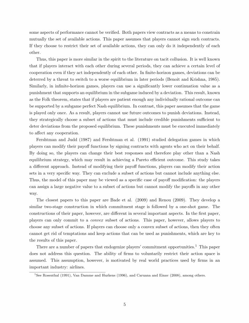
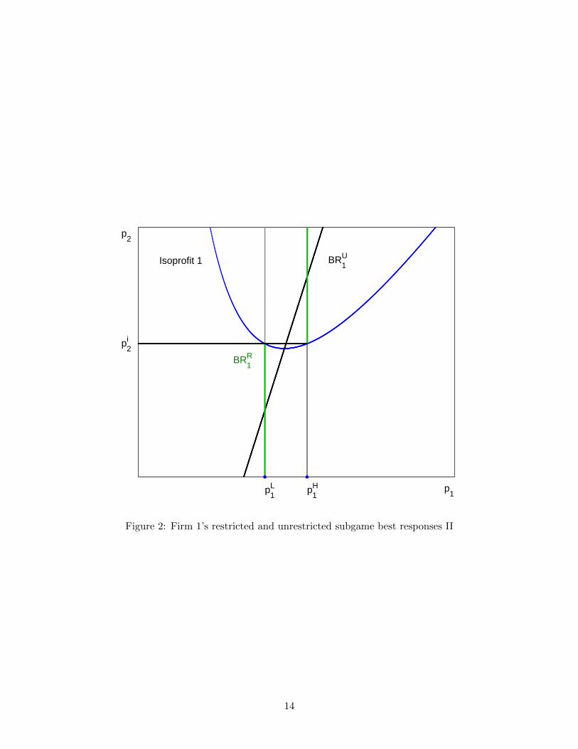
Second, suppose that two points from the image of the unconstrained subgame best response

BRi (A−i |Ai) belong to the restricted set Ai but the interval between them (ai, ai) does not. Then

there exists a vector of the competitors’ actions a−i such that both points of the interval belong

to the restricted subgame best response for this vector: {ai; ai} ∈ BRi (a−i |Ai) and the agent is

indifferent between playing either of them πi (ai, a−i) = πi (ai, a−i). Figure 2 illustrates this result

for the differentiated Bertrand duopoly with linear demand functions. Suppose that Firm 1 kept

two prices pL1 and pH1 but excluded the interval between them at the commitment stage. Then,

there exists a price pi2 such that if Firm 2 announces this price, Firm 1 will be indifferent between

charging prices pL1 and pH2 . The isoprofit crossing points(pL1 , p

i2

)and

(pH1 , p

i2

)illustrates this fact.

4See Appendix for the description of the model.

12

p1

p2

p1Hp

1L

BR1U

BR1R

Figure 1: Firm 1’s restricted and unrestricted subgame best responses I

13

p1

p2

p1H

p2i

p1L

BR1U

BR1R

Isoprofit 1

Figure 2: Firm 1’s restricted and unrestricted subgame best responses II

14

4.4 Subgame equilibrium response

For games with two players it is enough to analyze restricted subgame best responses. Indeed,

it is enough to check that the equilibrium action of the player maximizes her profit subject to

the fact that the opponent plays his restricted subgame best response. Formally, an outcome

a∗ = (a∗1, a∗2) ∈ A1 × A2 can be supported by a commitment equilibrium if and only if for each

player i and her action ai, it holds that πi (ai, a−i) ≤ πi (a∗) where a−i ∈ BR−i(ai|A∗−i

).

To analyze games with three or more players, looking at best responses is not enough. We need

to find a new equilibrium in each subgame induced by a possible deviation. Since more than one

player will react to the deviation, the subgame best responses have to take into account not only the

action of the deviator but also the reaction of the other players to this deviation. To take this into

account, we define a subgame equilibrium response as a function that for each possible deviation of

player i defines an equilibrium response of her opponents. Formally, function ER−i (ai|A−i) = a−i,

where (ai, a−i) is an equilibrium of the subgame for restricted sets Ai = {ai} and A−i. If there are

several equilibria in this subgame, ER−i chooses one for which πi (ai, a−i) is smallest. Using the

subgame equilibrium response function, we can formulate a necessary and sufficient condition for

a commitment equilibrium.

Proposition 2. A collection of restricted sets A∗i , i = 1, ...n can support an outcome a∗ ∈ A∗ by

a commitment equilibrium if and only if for each agent i and action ai, πi(a i, ER−i

(ai|A∗−i

))≤

πi(a∗i , a

∗−i).

Proof. If the inequality does not hold for some ai, then choosing ai at the commitment stage is a

profitable deviation for player i. So, we need only to show that the reverse is true. By Lemma 1, it

is enough to show that no profitable deviation to a singleton exists. Suppose it does and ai is such

a deviation. Then in the subgame induced by this deviation there is an equilibrium in which the

opponents of the deviator play a−i = ER−i(ai|A∗−i

). But since πi (ai, ER−i (ai|A∗i )) is less than

the equilibrium payoff for any ai, this deviation cannot be profitable.

Proposition 2 can be restated using the notion of a superior set. For each player i define a

superior set as Si (x) = {a ∈ A : πi (a) > πi (x)}. Then an outcome a∗ ∈ A can be supported

by a commitment equilibrium if and only if for all i the intersection of Si (a∗) and the graph of

ER−i (ai |A−i) is empty. The fact we just stated illustrates the role the commitment stage plays.

For a given outcome a ∈ A, the superior set Si (a∗) is fixed but the best response equilibrium

depends on the chosen restricted sets. To support a commitment equilibrium, the players have to

chose a collection of restricted action sets such that the graph of the resulting equilibrium response

does not overlap with the superior set.

4.5 Credibility of punishment

For a subgame supermodular game, the subgame best response is a nondecreasing correspondence.

This fact implies that ER−i (ai|A−i) is a nondecreasing function for any A−i. Consider the incen-

tives of player i to play an outcome a ∈ A as a commitment equilibrium. Suppose he decides to

15

deviate by playing a′i > ai. This deviation will not be profitable if πi (a′i, ER−i (a′i, A−i)) ≤ πi (a).

The same equality should hold if the deviator decides to increase its action. Thus, the payoff func-

tion cannot increase or decrease in all its arguments around the commitment equilibrium point.

Since the equilibrium response function is nondecreasing, only those outcomes for which the temp-

tation set for each player lies below the reward action, i.e. Ti (ai|Ai) ≤ ai for all i, can be supported

by a commitment equilibrium.

For a Bertrand oligopoly with differentiated products this property holds if the firms want to

support higher than NE prices. Indeed, when the prices exceed the NE, the profit of a potential

deviator will increase if he reduces its price but decrease if his competitors decide to do so.

Cournot duopolies,5 however, will violate this property. Suppose the firms want to support a

higher than monopoly price. To do so, they need to produce less. Thus, the deviator’s profit will

increase if he increases his output. To punish him, the firms have to increase their output further,

which will drive the price down. However, their best response to an increase in total output is to

decrease their own. Thus, in Cournot oligopolies, punishments that could have supported a high

price are not credible.

5 Stackelberg set

This section shows that there is, in fact, a set of payoff profiles that contains Pareto efficient

payoffs that can be supported by a commitment equilibrium. To define this set, we need to use

the concept of Stackelberg outcomes. An outcome aLi is called a Stackelberg outcome for player

i, if πi

(aLii , ER−i

(aLii

))≥ πi (ai, a−i) for any ai ∈ Ai. This outcome corresponds to a subgame

perfect equilibrium in the following modification of game G: player i moves first; the rest of the

players move simultaneously and independently of each other after observing the action of player i.

Similarly to a Nash equilibrium outcome, it is easy to establish that a Stackelberg outcome for any

player i can be supported by a commitment equilibrium. This equilibrium would prescribe that

players only choose their equilibrium action at the commitment stage. If all players do that, then

none will have an incentive to deviate either at the commitment stage or at the action stage.

Define the payoff of player i that corresponds to a Stackelberg outcome by πLii . The Stackelberg

set L is then defined as:

L ={a ∈ A: πi (a) ≥ πLi and Ti (a|Ai) ≤ ai for all i

}.

The previous literature has shown that the Stackelberg set L for a class of games is not empty (Amir

and Stepanova (2006) and Dowrick (1986)). Figure 3 shows the Stackelberg set for the Bertrand

duopoly with differentiated products and linear demands.

The next proposition shows that any outcome from the Stackelberg set can be supported by

5Generically, a Cournot oligopoly with three or more firms is not a supermodular game. However, it may becomeone under a set of reasonable assumptions placed on the market demand and cost functions (see, Amir, 1996). Theargument will still be true for games that satisfy these assumptions.

16

p1L

p2L

p1F

p2F

BR2

BR1

Isoprofit 2

Isoprofit 1

L

Figure 3: Stackelberg set

17

a commitment equilibrium if the players have an action that can serve as a credible punishment.

The proof of the proposition is constructive.

Proposition 3. Suppose for each player i, the payoff function πi is increasing in all a−i. Then an

outcome a∗ ∈ L can be supported by a commitment equilibrium if for any i there exists an action

aPi satisfying πi(aPi , a

∗−i)

= πi(a∗i , a

∗−i)

such that aPi ≤ BRi(a∗−i |Ai

).

Proof. Consider the following set of strategies. At the commitment stage each player includes in

A∗i the following elements: a∗i , aPi and all actions below aPi . To prove that a∗ can be supported by

a commitment equilibrium with these restricted sets, it is enough to show that for each player i

the graph of the equilibrium best response function and the superior set do not overlap.

First, consider the restricted subgame best responses. Based on the properties of the restricted

subgame best response established in Section 4.3, we can conclude that for a−i < aP−i, the best

response functions coincide. Then the restricted best response is equal to aPi until a∗−i. At a∗−i the

player is indifferent between playing aPi and a∗i . Finally, for a−i > a∗−i, player i will be playing a∗i .

Thus, the equilibrium response function will be the following: for ai ≥ a∗i , the other players will

play a∗−i, for ai < a∗i , they will play aP−i until ai ∈ BRi(aP−i|Ai

)and ER−i (ai|A−i) otherwise.

Since a∗ ∈ L, the superior set of player i belongs to the superior set constructed for the

Stackelberg outcome for player i, which in turn does not overlap with the unrestricted equilibrium

response function. For ai < a∗i the graph of the restricted equilibrium responses is bounded from

above by the unrestricted equilibrium response since aPi ≤ BRi(a∗−i|Ai

). Therefore, we need to

check that there are no overlaps for ai > a∗i . However, since the temptation set lies below a∗i , such

overlaps cannot exist.

The proposition shows that the punishment action has to satisfy the following property. Con-

ditional on the fact that all the opponents play the reward action, the player has to be indifferent

between playing his reward action and playing the punishment action. If a deviator follows his

temptation and includes an action from the temptation set, the other players will execute the pun-

ishment, which precludes the deviator from receiving any benefits from not choosing the reward.

6 Concluding comments

Motivated by pricing practices in the airline industry, this paper shows that in a competitive

environment, agents may benefit from committing not to play certain actions. For the commitment

equilibrium construction to work, all players should have commitment power and be able to play

several actions after the commitment stage. The main intuition of the paper is the following: to

get the reward, the players need to exclude all temptations but keep punishments to motivate their

opponents. Although the model is simple, its intuition can explain the otherwise puzzling menu

structure of airline fares.

There are several interesting extensions that could be further investigated. First, the model

assumed that the action stage was played only once. It is interesting to see what the players can

achieve when they can play the game a finite number of times. The commitment stage in this case

18

may provide punishments that players execute not only after deviations at the commitment stage

but also following deviations at the preceding action stages. Second, the trade-off becomes more

complicated when there is some uncertainty that is resolved between the commitment and action

stages. In this case, at the commitment stage the players do not know the exact punishment that

they will need to include and may end up including a non-credible punishment or a temptation.

Therefore, there is always a probability that the award action will not be an equilibrium at the

action stage along the equilibrium path. The third extension is more technical. Renou (2009)

shows an example of a game in which a mixed strategy Nash equilibrium does not survive in the

two-stage commitment game. Thus, the question is which mixed strategy equilibria can and which

cannot be supported by a commitment equilibrium.

19

References

Abreu, D., D. Pearce, and E. Stacchetti (1990): “Toward a Theory of Discounted Repeated

Games with Imperfect Monitoring,” Econometrica, 58, 1041–1063.

Amir, R. (1996): “Cournot Oligopoly and the Theory of Supermodular Games,” Games and

Economic Behavior, 15, 132–148.

Amir, R. and A. Stepanova (2006): “Second-mover advantage and price leadership in Bertrand

duopoly,” Games and Economic Behavior, 55, 1–20.

Bade, S., G. Haeringer, and L. Renou (2009): “Bilateral commitment,” Journal of Economic

Theory, 144, 1817–1831.

Benoit, J. and V. Krishna (1985): “Finitely Repeated Games,” Econometrica, 53, 905–922.

Bernheim, B. D. and M. D. Whinston (1998): “Incomplete Contracts and Strategic Ambigu-

ity,” The American Economic Review, 88, 902–932.

Caruana, G. and L. Einav (2008): “A Theory of Endogenous Commitment,” Review of Eco-

nomic Studies, 75, 99–116.

Dowrick, S. (1986): “von Stackelberg and Cournot Duopoly: Choosing Roles,” The RAND

Journal of Economics, 17, 251–260.

Fershtman, C. and K. L. Judd (1987): “Equilibrium Incentives in Oligopoly,” The American

Economic Review, 77, 927–940.

Fershtman, C., K. L. Judd, and E. Kalai (1991): “Observable Contracts: Strategic Delegation

and Cooperation,” International Economic Review, 32, 551–559.

Fudenberg, D. and E. Maskin (1986): “The Folk Theorem in Repeated Games with Discounting

or with Incomplete Information,” Econometrica, 54, 533–554.

Hart, O. and J. Moore (2004): “Agreeing Now to Agree Later: Contracts that Rule Out but

do not Rule In,” National Bureau of Economic Research Working Paper Series, No. 10397.

Milgrom, P. and J. Roberts (1990): “Rationalizability, learning, and equilibrium in games

with strategic complementarities,” Econometrica, 58, 1255–1277.

Nash, J. F. (1950): “Equilibrium points in n-person games,” Proceedings of the National Academy

of Sciences of the United States of America, 48–49.

Renou, L. (2009): “Commitment games,” Games and Economic Behavior, 66, 488–505.

Reny, P. J. (1999): “On the existence of pure and mixed strategy Nash equilibria in discontinuous

games,” Econometrica, 67, 1029–1056.

20

Rosenthal, R. W. (1991): “A note on robustness of equilibria with respect to commitment

opportunities,” Games and Economic Behavior, 3, 237–243.

Schelling, T. C. (1960): The strategy of conflict, Harvard University Press.

Silk, A. and S. Michael (1993): “American Airlines Value Pricing (A),” Harvard Business

School Case Study 9-594-001. Cambridge, MA: Harvard Business School Press.

Topkis, D. M. (1979): “Equilibrium points in nonzero-sum n-person submodular games,” SIAM

Journal on Control and Optimization, 17, 773.

van Damme, E. and S. Hurkens (1996): “Commitment Robust Equilibria and Endogenous

Timing,” Games and Economic Behavior, 15, 290–311.

Vives, X. (1990): “Nash equilibrium with strategic complementarities,” Journal of Mathematical

Economics, 19, 305–321.

21

A Commitment equilibrium in Bertrand duopoly with differenti-

ated products

To illustrate the idea of a commitment game, consider the differentiated Bertrand duopoly model

with linear demand functions. Suppose two symmetric firms (i = 1,2) produce differentiated

products. The demand for each product depends both on its price and the price of the competitor

in a linear way:

q1 (p1, p2) = 1− p1 + αp2,

q2 (p1, p2) = 1− p2 + αp1,

where α ∈ (0, 1) is the parameter that characterizes the degree of products’ substitutability: the

higher is α, the more substitutable are the products.

If firms set their prices simultaneously and independently, then there exists a unique Nash

equilibrium in which both firms charge the following price:

pNE1 = pNE2 =1

2− α.

As a result, both firms receive profits equal to πNE1 = πNE2 = 1(2−α)2 .

It is easy to see that this pair of profits does not lie on the Pareto frontier. In other words, if

both firms decide to increase their price by a small amount (ε > 0), then both profits will increase:

π1 = π2 =1

(2− α)2+

α

2− αε− (1− α) ε2 >

1

(2− α)2

for small ε > 0.

Thus, if the firms could agree to coordinate their actions, they could do better. Yet, it is clear

that neither firm unilaterally has an incentive to declare it will charge the profit maximizing price

pM1 = pM2 = 12(1−α) . To see why this pair of prices cannot be a Nash equilibrium, consider the

figure.

The figure depicts the isoprofit curves for each firm corresponding to the prices that maximize

the firms’ joint profit. These isoprofits touch each other at(

12(1−α) ,

12(1−α)

), the point that max-

imizes the firms’ joint profit. Suppose firm 1 knows that firm 2 will charge pM2 . If firm 1 charges

pM1 , then it gets πM1 = 14(1−α) . However, if firm 1 charges a different price, in particular, any price

in the range(pP1 , p

M1

), then its profit will be strictly higher than πM1 . In other words, firm 1 has a

temptation to deviate from the price it is supposed to charge and charge something lower. Unless

firm 1 can commit not to charge prices from the interval(pP1 , p

M1

), the pair of prices

(pM1 , p

M2

)cannot be an equilibrium.

Suppose now that firms have ability to restrain themselves independently of each other. To

be more precise, suppose that firms choose a subset of their prices first. We saw that firm 1 can

profitably deviate if it charges any price from(pP1 , p

M1

). Therefore, in an equilibrium it needs

22

Figure 4: Differentiated Bertrand Duopoly. How to Support a Joint-Profit Maximizing Outcome

23

to restrain itself and exclude all prices from that interval. However, it has an incentive to cheat

(a ”temptation”). Therefore firm 2 has to be able to punish firm 1 if it includes prices from that

interval. Hence, firm 2 has to choose not only price pM2 that it is supposed to play in an equilibrium

but also some other prices that it will use as punishments should firm 1 not commit to exclude

prices in the interval(pP1 , p

M1

).

For reasons discussed in the main text, it is sufficient in this case for each firm to choose just

two prices: the pair of prices that will be played along the equilibrium path(pM1 , p

M2

)and two

prices that will be used as punishments, namely pP1 and pP2 . To see why committing to just two

prices in an initial stage will work, suppose firm 1 decides to deviate and restrains itself to some

other price. It is easy to verify that firm 2 will charge pM2 if firm 1 charges any price higher than

pM1 . If firm 1 charges any price lower than pM1 , then firm 2 should choose pP2 . Thus, firm 1 cannot

benefit from a deviation given firm 2 commits to{pM2 , p

P2

}since the isoprofit of firm 1 lies to the

north of firm 2’s optimal response. Perhaps, however, firm 1 could benefit from choosing more than

one price at the commitment stage? It turns out that no matter what subset of prices the firm

chooses, there will always exist a pure-strategy Nash equilibrium in the corresponding subgame in

which firm 2 will play either pM2 or pP2 . In neither case, as we already have seen, can firm 1 benefit

if it deviates.

Thus, in this widely studied game, if firms can restrain themselves independently of each other,

they can coordinate on the outcome that maximizes their joint profit.

24