arX

iv:1

507.

0147

8v1

[m

ath.

PR]

6 J

ul 2

015

Asymmetric stochastic transport models

with Uq(su(1, 1)) symmetry

Gioia Carinci(a), Cristian Giardina(a),Frank Redig(b), Tomohiro Sasamoto (c).

(a) Department of Mathematics, University of Modena and Reggio Emilia

via G. Campi 213/b, 41125 Modena, Italy(b) Delft Institute of Applied Mathematics, Technische Universiteit Delft

Mekelweg 4, 2628 CD Delft, The Netherlands(c) Department of Physics, Tokyo Institute of Technology,

2-12-1 Ookayama, Meguro-ku, Tokyo, 152-8550, Japan

August 28, 2018

Abstract

By using the algebraic construction outlined in [10], we introduce several Markovprocesses related to the Uq(su(1, 1)) quantum Lie algebra. These processes serve asasymmetric transport models and their algebraic structure easily allows to deduce dualityproperties of the systems. The results include: (a) the asymmetric version of the InclusionProcess, which is self-dual; (b) the diffusion limit of this process, which is a naturalasymmetric analogue of the Brownian Energy Process and which turns out to have thesymmetric Inclusion Process as a dual process; (c) the asymmetric analogue of the KMPProcess, which also turns out to have a symmetric dual process. We give applications ofthe various duality relations by computing exponential moments of the current.

1

Contents

1 Introduction 3

1.1 Motivations . . . . . . . . . . . . . . . . . . . . . . . . . . . . . . . . . . . . . 31.2 Models and abbreviations . . . . . . . . . . . . . . . . . . . . . . . . . . . . . 31.3 Markov processes with algebraic structure . . . . . . . . . . . . . . . . . . . . 41.4 Informal description of main results . . . . . . . . . . . . . . . . . . . . . . . 41.5 Organization of the paper . . . . . . . . . . . . . . . . . . . . . . . . . . . . . 5

2 The Asymmetric Inclusion Process ASIP(q, k) 5

2.1 Basic notation . . . . . . . . . . . . . . . . . . . . . . . . . . . . . . . . . . . 52.2 The ASIP(q, k) process . . . . . . . . . . . . . . . . . . . . . . . . . . . . . . . 62.3 Limiting cases . . . . . . . . . . . . . . . . . . . . . . . . . . . . . . . . . . . . 72.4 Reversible profile product measures . . . . . . . . . . . . . . . . . . . . . . . . 8

3 The Asymmetric Brownian Energy Process ABEP(σ, k) 9

3.1 Definition . . . . . . . . . . . . . . . . . . . . . . . . . . . . . . . . . . . . . . 103.2 Limiting cases . . . . . . . . . . . . . . . . . . . . . . . . . . . . . . . . . . . . 113.3 The ABEP(σ, k) as a diffusion limit of ASIP(q, k). . . . . . . . . . . . . . . . 123.4 Reversible measure of the ABEP(σ, k) . . . . . . . . . . . . . . . . . . . . . . 143.5 Transforming the ABEP(σ, k) to BEP(k) . . . . . . . . . . . . . . . . . . . . 153.6 The algebraic structure of ABEP(σ, k) . . . . . . . . . . . . . . . . . . . . . . 18

4 The Asymmetric KMP process, AKMP(σ) 19

4.1 Instantaneous Thermalizations . . . . . . . . . . . . . . . . . . . . . . . . . . 194.2 Thermalized Asymmetric Inclusion process Th-ASIP(q, k) . . . . . . . . . . . 204.3 Thermalized Asymmetric Brownian energy process Th-ABEP(σ, k). . . . . . . 21

5 Duality relations 24

5.1 Self-duality of ASIP(q, k) . . . . . . . . . . . . . . . . . . . . . . . . . . . . . 255.2 Duality between ABEP(σ, k) and SIP(k) . . . . . . . . . . . . . . . . . . . . . 265.3 Duality for the instantaneous thermalizations . . . . . . . . . . . . . . . . . . 27

6 Applications to exponential moments of currents 28

6.1 Infinite volume limit for ASIP(q, k) . . . . . . . . . . . . . . . . . . . . . . . . 296.2 q-exponential moment of the current of ASIP(q, k) . . . . . . . . . . . . . . . 326.3 Infinite volume limit for ABEP(σ, k) . . . . . . . . . . . . . . . . . . . . . . . 366.4 e−σ-exponential moment of the current of ABEP(σ, k) . . . . . . . . . . . . . 37

7 Algebraic construction of ASIP(q, k) and proof of the self-duality 40

7.1 Algebraic structure and symmetries . . . . . . . . . . . . . . . . . . . . . . . . 407.2 Construction of ASIP(q, k) from the quantum Hamiltonian . . . . . . . . . . 457.3 Self-Duality of ASIP(q, k) . . . . . . . . . . . . . . . . . . . . . . . . . . . . . 49

2

1 Introduction

1.1 Motivations

Exactly solvable stochastic systems out-of-equilibrium have received considerable attentionin recent days [27, 16, 11, 24, 6, 5]. Often in the analysis of these models duality (or self-duality) is a crucial ingredient by which the study of n-point correlations is reduced tothe study of n dual particles. For instance, the exact current statistics in the case of theasymmetric exclusion process is obtained by solving the dual particle dynamics via Betheansatz [26, 18, 4].

The duality property has algebraic roots, as was first noticed by Schutz and Sandow forsymmetric exclusion processes [25], which is related to the classical Lie algebra su(2). Nextthis symmetry approach was extended by Schutz [26] to the quantum Lie algebra Uq(su(2)) ina representattion of spin 1/2, thus providing self-duality of the asymmetric exclusion process.Recently Markov processes with the Uq(su(2)) algebraic structure for higher spin value havebeen introduced and studied in [10]. This lead to a family of non-integrable asymmetricgeneralization of the partial exclusion process (see also [22]).

In [13, 14] the algebraic approach to duality has been extended by connecting dualityfunctions to the algebra of operators commuting with the generator of the process. In par-ticular for the models of heat conduction studied in [14] the underlying algebraic structureturned out to be U (su(1, 1)). This class is richer than its fermionic counterpart related tothe classical Lie algebra U (su(2)) which is at the root of processes of exclusion type. Inparticular, the classical Lie algebra U (su(1, 1)) has been shown to be related to a large classof symmetric processes, including: (a) an interacting particle system with attractive inter-actions (inclusion process [14, 15]); (b) interacting diffusion processes for heat conduction(Brownian energy process [14, 9]); (c) redistribution models of KMP-type [19, 8]. The dua-lities and self-dualities of all these processes arise naturally from the symmetries which arebuilt in the construction.

It is the aim of this paper to provide the asymmetric version of these models with (self)-duality property, via the study of the deformed quantum Lie algebra Uq(su(1, 1)). Thisprovides a new class of bulk-driven non-equilibrium systems with duality, which includes inparticular an asymmetric version of the KMP model [19]. The diversity of models related tothe classical U (su(1, 1)) will also appear here in the asymmetric context where we considerthe quantum Lie algebra Uq(su(1, 1)).

1.2 Models and abbreviations

For the sake of simplicity, we will use the following acronyms in order to describe the classof new processes that arise from our construction.

(a) Discrete representations will provide interacting particle systems in the class of InclusionProcesses. For a parameter k ∈ R+, the Symmetric Inclusion Process version is denotedby SIP(k), and ASIP(q, k) is the corresponding asymmetric version, with asymmetryparameter q ∈ (0, 1).

(b) Continuous representations give rise to diffusion processes in the class of BrownianEnergy Processes. For k ∈ R+, the Symmetric Brownian Energy Process is denoted by

3

BEP(k), and ABEP(σ, k) is the asymmetric version with asymmetry parameter σ > 0.

(c) By instantaneous thermalization, redistribution models are obtained, where energy orparticles are redistributed at Poisson event times. This class includes the thermal-ized version of ABEP(σ, k), which is denoted by Th-ABEP(σ, k). In the particularcase k = 1/2 the Th-ABEP(σ, k) is called the asymmetric KMP (Kipnis-Marchioro-Presutti) model, denoted by AKMP(σ), which becomes the KMP model as σ → 0.The instantaneous thermalization of the ASIP(q, k) yields the Th-ASIP(q, k) process.

1.3 Markov processes with algebraic structure

In [10] we constructed a generalization of the asymmetric exclusion process, allowing 2jparticles per site with self-duality properties reminiscent of the self-duality of the standardASEP found initially by Schutz in [26]. This construction followed a general scheme whereone starts from the Casimir operator C of the quantum Lie algebra Uq(su(2)), and appliesa coproduct to obtain an Hamiltonian Hi,i+1 working on the occupation number variables

at sites i and i + 1. The operator H =∑L

i=1Hi,i+1 then naturally allows a rich classof commuting operators (symmetries), obtained from the n-fold coproduct applied to anygenerator of the algebra. This operator H is not yet the generator of a Markov process. ButH allows a strictly positive ground state, which can also be constructed from the symmetriesapplied to a trivial ground state. Via a ground state transformation, H can then be turnedinto a Markov generator L of a jump process where particles hop between nearest neighborsites and at most 2j particles per site are allowed. The symmetries of H directly translateinto the symmetries of L, which in turn directly translate into self-duality functions.

This construction is in principle applicable to every quantum Lie algebra with a non-trivial center. However, it is not guaranteed that a Markov generator can be obtained. Thisdepends on the chosen representation of the generators of the algebra, and the choice of theco-product. Recently the construction has been applied to algebras with higher rank, suchas Uq(gl(3)) [3, 20] or Uq(sp(4)) [20], yielding two-component asymmetric exclusion processwith multiple conserved species of particles.

1.4 Informal description of main results

In [14] we introduced a class of processes with su(1, 1) symmetry which in fact arise from thisconstruction for the Lie algebra U (su(1, 1)). In this paper we look for natural asymmetricversions of the processes constructed in [14], and [8]. In particular the natural asymmetricanalogue of the KMP process is a target. The main results are the following

(a) Self-duality of ASIP(q, k). We proceed via the same construction as in [10] for thealgebra Uq(su(1, 1)) to find the ASIP(q, k) which is the “correct” asymmetric analogueof the SIP(k). The parameter q tunes the asymmetry: q → 1 gives back the SIP(k).This process is then via its construction self-dual with a non-local self-duality function.

(b) Duality between ABEP(σ, k) and SIP(k). We then show that in the limit ǫ → 0 wheresimultaneously the asymmetry is going to zero (q = 1 − ǫσ tends to unity), and thenumber of particles to infinity ηi = ⌊ǫ−1xi⌋, we obtain a diffusion process ABEP(σ, k)which is reminiscent of the Wright-Fisher diffusion with mutation and a selective drift.

4

As a consequence of self-duality of ASIP(q, k) we show that this diffusion process is dualto the SIP(k), i.e., the dual process is symmetric, and the asymmetry is in the dualityfunction. Notice that this is the first example of duality between a truly asymmetricsystem (i.e. bulk-driven) and a symmetric system (with zero current).

(c) Duality of instantaneous thermalization models. Finally, we then consider instantaneousthermalization of ABEP(σ, k) to obtain an asymmetric energy redistribution model ofKMP type. Its dual is the instantaneous thermalization of the SIP(k) which for k = 1/2is exactly the dual KMP process.

1.5 Organization of the paper

The rest of our paper is organized as follows. In section 2 we introduce the process ASIP(q, k).After discussing some limiting cases, we show that this process has reversible profile productmeasures on Z+ (but not on Z).

In section 3 we consider the weak asymmetry limit of ASIP(q, k). This leads to thediffusion process ABEP(σ, k), that also has reversible inhomogeneous product measures onthe half-line. We prove that ABEP(σ, k) is a genuine non-equilibrium asymmetric system inthe sense that it has a non-zero average current. Nevertheless in the last part of section 3we show that the ABEP(σ, k) can be mapped – via a global change of coordinates – to theBEP(k), which is a symmetric system with zero-current. In section 3.6 this is also explainedin the framework of the representation theory of the classical Lie algebra U (su(1, 1)).

In section 4 we introduce the instantaneous thermalization limits of both ASIP(q, k) andABEP(σ, j) which are a particle, resp. energy, redistribution model at Poisson event times.This provides asymmetric redistribution models of KMP type.

In section 5 we introduce the self-duality of the ASIP(q, k) and prove various other dualityrelations that follow from it. In particular, once the self-duality of ASIP(q, k) is obtained,duality of ABEP(σ, k) with SIP(k) follows from a limiting procedure which is proved inSection 5.2. In the limit of an infinite number of particles with weak-asymmetry, the originalprocess scales to ABEP(σ, k), whereas in the dual process the asymmetry disappears becausethe number of particles is finite. Next the self-duality and duality of thermalized models isderived in Section 5.3.

In section 6 we illustrate the use of the duality relations in various computations ofexponential moments of currents. Finally, the last section is devoted to the full constructionof the ASIP(q, k) from a Uq(su(1, 1)) symmetric quantum Hamiltonian and the proof of self-duality from the symmetries of this Hamiltonian.

2 The Asymmetric Inclusion Process ASIP(q, k)

2.1 Basic notation

We will consider as underlying lattice the finite lattice ΛL = 1, . . . , L or the periodic latticeTL = Z/LZ. At the sites of ΛL we allow an arbitrary number of particles. The particlesystem configuration space is ΩL = NΛL . Elements of ΩL are denoted by η, ξ and for η ∈ ΩL,i ∈ ΛL, we denote by ηi ∈ N the number of particles at site i. For η ∈ ΩL and i, j ∈ ΛL suchthat ηi > 0, we denote by ηi,j the configuration obtained from η by removing one particle

5

from i and putting it at j.

We need some further notation of q-numbers. For q ∈ (0, 1) and n ∈ N0 we introduce theq-number

[n]q =qn − q−n

q − q−1(2.1)

satisfying the property limq→1[n]q = n. The first q-number’s are thus given by

[0]q = 0, [1]q = 1, [2]q = q + q−1, [3]q = q2 + 1 + q−2, . . .

We also introduce the q-factorial

[n]q! := [n]q · [n− 1]q · · · · · [1]q ,

and the q-binomial coefficient(n

m

)

q

:=[n]q!

[m]q![n −m]q!.

Further we denote(a; q)m := (1− a)(1− aq) · · · (1− aqm−1) . (2.2)

2.2 The ASIP(q, k) process

We introduce the process in finite volume by specifying its generator.

DEFINITION 2.1 (ASIP(q,k) process).

1. The ASIP(q, k) with closed boundary conditions is defined as the Markov process on ΩLwith generator defined on functions f : ΩL → R

(LASIP (q,k)(L) f)(η) :=

L−1∑

i=1

(LASIP (q,k)i,i+1 f)(η) with

(LASIP (q,k)i,i+1 f)(η) := qηi−ηi+1+(2k−1)[ηi]q[2k + ηi+1]q(f(η

i,i+1)− f(η))

+ qηi−ηi+1−(2k−1)[2k + ηi]q[ηi+1]q(f(ηi+1,i)− f(η)) (2.3)

2. The ASIP(q, k) with periodic boundary conditions is defined as the Markov process onNTL with generator

(LASIP (q,k)(TL) f)(η) :=

∑

i∈TL

(LASIP (q,k)i,i+1 f)(η) (2.4)

Since in finite volume we always start with finitely many particles, and the total particle num-ber is conserved, the process is automatically well defined as a finite state space continuoustime Markov chain. Later on (see Section 6.1) we will consider expectations of the self-dualityfunctions in the infinite volume limit. In this way we can deal with relevant infinite volumeexpectations without having to solve the full existence problem of the ASIP(q, k) in infinitevolume for a generic initial data. This might actually be an hard problem due to the lack ofmonotonicity.

6

2.3 Limiting cases

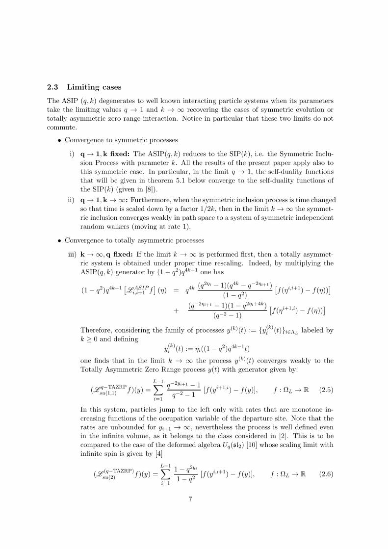
The ASIP (q, k) degenerates to well known interacting particle systems when its parameterstake the limiting values q → 1 and k → ∞ recovering the cases of symmetric evolution ortotally asymmetric zero range interaction. Notice in particular that these two limits do notcommute.

• Convergence to symmetric processes

i) q → 1,k fixed: The ASIP(q, k) reduces to the SIP(k), i.e. the Symmetric Inclu-sion Process with parameter k. All the results of the present paper apply also tothis symmetric case. In particular, in the limit q → 1, the self-duality functionsthat will be given in theorem 5.1 below converge to the self-duality functions ofthe SIP(k) (given in [8]).

ii) q → 1,k → ∞: Furthermore, when the symmetric inclusion process is time changedso that time is scaled down by a factor 1/2k, then in the limit k → ∞ the symmet-ric inclusion converges weakly in path space to a system of symmetric independentrandom walkers (moving at rate 1).

• Convergence to totally asymmetric processes

iii) k → ∞,q fixed: If the limit k → ∞ is performed first, then a totally asymmet-ric system is obtained under proper time rescaling. Indeed, by multiplying theASIP(q, k) generator by (1− q2)q4k−1 one has

(1− q2)q4k−1[L ASIPi,i+1 f

](η) = q4k

(q2ηi − 1)(q4k − q−2ηi+1)

(1− q2)

[f(ηi,i+1)− f(η))

]

+(q−2ηi+1 − 1)(1 − q2ηi+4k)

(q−2 − 1)

[f(ηi+1,i)− f(η))

]

Therefore, considering the family of processes y(k)(t) := y(k)i (t)i∈ΛLlabeled by

k ≥ 0 and defining

y(k)i (t) := ηi((1− q2)q4k−1t)

one finds that in the limit k → ∞ the process y(k)(t) converges weakly to theTotally Asymmetric Zero Range process y(t) with generator given by:

(L q−TAZRPsu(1,1) f)(y) =

L−1∑

i=1

q−2yi+1 − 1

q−2 − 1[f(yi+1,i)− f(y)], f : ΩL → R (2.5)

In this system, particles jump to the left only with rates that are monotone in-creasing functions of the occupation variable of the departure site. Note that therates are unbounded for yi+1 → ∞, nevertheless the process is well defined evenin the infinite volume, as it belongs to the class considered in [2]. This is to becompared to the case of the deformed algebra Uq(sl2) [10] whose scaling limit withinfinite spin is given by [4]

(L(q−TAZRP)su(2)

f)(y) =L−1∑

i=1

1− q2yi

1− q2[f(yi,i+1)− f(y)], f : ΩL → R (2.6)

7

Here particles jump to the right only with rates that are also a monotonous in-creasing function of the occupation variable of the departure site, however now itis a bounded function approaching 1 in the limit yi → ∞. In [12] it is proved thatthe totally asymmetric zero range process (2.6) is in the KPZ universality class.It is an interesting open problem to prove or disprove that the same conclusionholds true for (2.5) [23]. We remark that the rates of (2.5) are (discrete) convexfunction and this also translates into convexity of the stationary current j(ρ) as afunction of the density ρ, whereas for (2.6) we have concave relations.

iv) k → ∞,q → 1: In the limit q → 1 the zero range process in (2.5) reduces to asystem of totally asymmetric independent walkers. This is to be compared to itemii) where symmetric walkers were found if the two limits were performed in thereversed order.

2.4 Reversible profile product measures

Here we describe the reversible measures of ASIP(q, k).

THEOREM 2.1 (Reversible measures of ASIP(q, k)). For all L ∈ N, L ≥ 2, the followingresults hold true:

1.) the ASIP(q, k) on ΛL with closed boundary conditions admits a family labeled by α ofreversible product measures with marginals given by

P(α)(ηi = n) =αn

Z(α)i

(n+ 2k − 1

n

)

q

· q4kin n ∈ N (2.7)

for i ∈ ΛL and α ∈ [0, q−(2k+1)) (with the convention(2k−1

0

)q= 1). The normalization

is

Z(α)i =

+∞∑

n=0

(n+ 2k − 1

n

)

q

· αnq4kin =1

(αq4ki−(2k−1); q2)2k(2.8)

and for this measure

E(α)(ηi) =

2k−1∑

l=0

1

q−2l(αq4ki−2k+1)−1 − 1. (2.9)

2.) The ASIP(q, k) process on the torus TL with periodic boundary condition does not admithomogeneous product measures.

PROOF. The proof of item 2.) is similar to the proof of Theorem 3.1, item d) in [10] and werefer the reader to that paper for all details. To prove item 1.) consider the detailed balancerelation

µ(η)cq(η, ηi,i+1) = µ(ηi,i+1)cq(η

i,i+1, η) (2.10)

where the hopping rates are given by

cq(η, ηi,i+1) = qηi−ηi+1+2k−1[ηi]q[2k + ηi+1]q

8

cq(ηi,i+1, η) = qηi−ηi+1−2k−1[2k + ηi − 1]q[ηi+1 + 1]q

and µ denotes a reversible measure. Suppose now that µ is a product measure of the formµ = ⊗L

i=1µi. Then (2.10) holds if and only if

µi(ηi−1)µi+1(ηi+1+1)q−2k[2k+ηi−1]q[ηi+1+1]q = µi(ηi)µi+1(ηi+1)q2k[ηi]q[2k+ηi+1]q (2.11)

which implies that there exists α ∈ R so that for all i ∈ ΛL

µi(n)

µi(n− 1)= αq4ki

[2k + n− 1]q[n]q

. (2.12)

Then (2.7) follows from (2.12) after using an induction argument on n. The normalization

Z(α)i is computed by using Corollary 10.2.2 of [1]. We have that

Z(α)i <∞ if and only if 0 ≤ α < q−4ki+(2k−1) for any i ∈ ΛL (2.13)

As a consequence (since q < 1 and i = 1 is the worst case) α must belong to the interval[0, q−(2k+1)). The expectation (2.9) is obtained by exploiting the identity

E(α)(ηi) = αd

dαlogZ

(α)i .

The following comments are in order:

i) vanishing asymmetry: in the limit q → 1 the reversible product measure of ASIP(q, k)converges to a product of Negative Binomial distributions with shape parameter 2k andsuccess probability α, which are the reversible measures of the SIP(k) [8].

ii) monotonicity of the profile: the average occupation number E(α)(ηi) in formula (2.9) isa decreasing function of i, and limi→∞ E(α)(ηi) = 0.

iii) infinite volume: the reversible product measures with marginal (2.7) are also well-defined in the limit L → ∞. One could go further to [−M,∞) ∩ Z for α < q4kM+2k−1

(but not to the full line Z). These infinite volume measure concentrate on configurationswith a finite number of particles, and thus are the analogue of the profile measures inthe asymmetric exclusion process [21].

3 The Asymmetric Brownian Energy Process ABEP(σ, k)

Here we will take the limit of weak asymmetry q = 1 − ǫσ → 1 (ǫ → 0) combined with thenumber of particles proportional to ǫ−1, going to infinity, and work with rescaled particlenumbers xi = ⌊ǫηi⌋. Reminiscent of scaling limits in population dynamics, this leads to adiffusion process of Wright-Fisher type [9], with σ-dependent drift term, playing the roleof a selective drift in the population dynamics language, or bulk driving term in the non-equilibrium statistical physics language.

9

3.1 Definition

We define the ABEP(q, k) process via its generator. It has state space XL = (R+)L, R+ :=

[0,+∞). Configurations are denoted by x ∈ XL, with xi being interpreted as the energy atsite i ∈ ΛL.

DEFINITION 3.1 (ABEP(σ, k) process).

1. Let σ > 0 and k ≥ 0. The Markov process ABEP(σ, k) on the state space XL withclosed boundary conditions is defined by the generator working on the core of smoothfunctions f : XL → R via

[L ABEP (σ,k)

(L) f ](x) =

L−1∑

i=1

[L ABEP (σ,k)

i,i+1 f ](x) (3.1)

with

[L ABEP (σ,k)

i,i+1 f](x) =

1

4σ2(1− e−2σxi)(e2σxi+1 − 1)

(∂

∂xi− ∂

∂xi+1

)2

f(x)

− 1

2σ

(1− e−2σxi)(e2σxi+1 − 1) + 2k

(2− e−2σxi − e2σxi+1

)( ∂

∂xi− ∂

∂xi+1

)f(x)

2. The ABEP(σ, k) with periodic boundary conditions is defined as the Markov process onRTL+ with generator

[LABEP (σ,k)(TL)

f ](x) :=∑

i∈TL

[LABEP (σ,k)i,i+1 f ](x) (3.2)

The ABEP(σ, k) is a genuine asymmetric non-equilibrium system, in the sense that itstranslation-invariant stationary state may sustain a non-zero current. To see this, let E

denote expectation with respect to the translation invariant measure for the ABEP(σ, k) onTL. Let fi(x) := xi, then from (3.2) we have

[L ABEP (σ,k)fi](x) = Θi,i+1(x)−Θi−1,i(x) (3.3)

with

Θi,i+1(x) = − 1

2σ

(1− e−2σxi)(e2σxi+1 − 1) + 2k

(2− e−2σxi − e2σxi+1

)(3.4)

So we haved

dtEx [fi(x(t))] = Ex [Θi,i+1(x(t))] − Ex [Θi−1,i(x(t))]

and then, from the continuity equation we have that, in a translation invariant state, Ji,i+1 :=−E [Θi,i+1] is the instantaneous stationary current over the edge (i, i+1). Thus we have thefollowing

10

PROPOSITION 3.1 (Non-zero current of ABEP(σ, k)).

Ji,i+1 = −E [Θi,i+1] < 0 if k > 1/2

andJi,i+1 = −E [Θi,i+1] > 0 if k = 0 .

PROOF. In the case k > 1/2, taking expectation of (3.4) we obtain

E [Θi,i+1] =1

2σ

(1− 4k) + (2k − 1)E(e2σxi+1 + e−2σxi) + E(e2σ(xi+1−xi))

Since expectation in the translation invariant stationary state of local variables are the sameon each site and cosh(x) ≥ 1 one obtains

E [Θi,+1] ≥1

2σ

(1− 4k) + 2(2k − 1) + E

[e2σ(xi+1−xi)

]

Furthermore, Jensen inequality and translation invariance implies that

E [Θi,i+1] >1

2σ

(1− 4k) + 2(2k − 1) + 1

= 0

In the case k = 0 one has

E [Θi,i+1] =1

2σE[(1− e−2σxi)(1 − e2σxi+1)

]< 0

which is negative because the function is negative a.s.

3.2 Limiting cases

• Symmetric processes

i) σ → 0,k fixed: we recover the Brownian Energy Process with parameter k,BEP(k) (see [8]) whose generator is

L BEP (k)

i,i+1 = xixi+1

(∂

∂xi− ∂

∂xi+1

)2

− 2k(xi − xi+1)

(∂

∂xi− ∂

∂xi+1

)(3.5)

ii) σ → 0,k → ∞: under the time rescaling t → t/2k, one finds that in the limitk → ∞ the BEP(k) process scales to a symmetric deterministic system evolvingwith generator

[L DEPi,i+1 f

](x) = −(xi − xi+1)

(∂

∂xi− ∂

∂xi+1

)f(x) (3.6)

This deterministic system is symmetric in the sense that if the initial condition isgiven by (xi(0), xi+1(0)) = (a, b) then the asymptotic solution is given by the fixedpoint

(a+b2 , a+b2

)where the initial total energy a+ b is equally shared among the

two sites.

11

• Wright-Fisher diffusion

iii) σ ≃ 0,k fixed: the ABEP(σ, k) on the simplex can be read as a Wright Fishermodel with mutation and selection, however we have not been able to find in theliterature the specific form of selection appearing in (3.2) (see [9] for the analogousresult when σ = 0). To first order in σ one recovers the standard Wright-Fishermodel with constant mutation k and selection σ

LWF (σ,k) = xixi+1

(∂

∂xi− ∂

∂xi+1

)2

− (2σxixi+1 + 2k(xi − xi+1))

(∂

∂xi− ∂

∂xi+1

)

• Asymmetric Deterministic System

iv) k → ∞, σ fixed: if the limit k → ∞ is taken directly on the ABEP(σ, k) then, bytime rescaling t → t/2k one arrives at an asymmetric deterministic system withgenerator

L ADEP (σ)

i,i+1 = − 1

2σ

(2− e−2σxi − e2σxi+1

)( ∂

∂xi− ∂

∂xi+1

)(3.7)

This deterministic system is asymmetric in the sense that if the initial conditionis given by (xi(0), xi+1(0)) = (a, b) then the asymptotic solution is given by thefixed point

(A,B) :=

(1

2σln

(1 + e2σ(a+b)

2

), a+ b− 1

2σln

(1 + e2σ(a+b)

2

))

where A > B.

v) k → ∞, σ → 0: in the limit σ → 0 (3.7) converges to (3.6) and one recoversagain the symmetric equi-distribution between the two sites of DEP process withgenerator (3.6).

vi) k → ∞, σ → ∞: in the limit σ → ∞ one has the totally asymmetric stationarysolution (a+ b, 0).

3.3 The ABEP(σ, k) as a diffusion limit of ASIP(q, k).

Here we show that the ABEP(σ, k) arises from the ASIP(q, k) in a limit of vanishing asym-metry and infinite particle number.

THEOREM 3.1 (Weak asymmetry limit of ASIP(q, k)). Fix T > 0. Let ηǫ(t) : 0 ≤ Tdenote the ASIP(1− σǫ, k) starting from initial condition ηǫ(0). Assume that

limǫ→0

ǫηǫ(0) = x ∈ XL (3.8)

Then as ǫ → 0, the process ηǫ(t) : 0 ≤ t ≤ T converges weakly on path space to theABEP(σ, k) starting from x.

12

PROOF. The proof follows the lines of the corresponding results in population dynamicsliterature, i.e., Taylor expansion of the generator and keeping the relevant orders. Indeed,by the Trotter-Kurtz theorem [21], we have to prove that on the core of the generator of thelimiting process, we have convergence of generators. Because the generator is a sum of termsworking on two variables, our theorem follows from the computational lemma below.

LEMMA 3.1. If ηǫ ∈ ΩL is such that ǫηǫ → x ∈ XL then, for every smooth function F :XL → R, and for every i ∈ 1, . . . , L− 1 we have

limǫ→0

(LASIP (1−ǫσ,k)i,i+1 Fǫ)(η

ǫ) = LABEP (σ,k)i,i+1 F (x) (3.9)

where Fǫ(η) = F (ǫη), η ∈ ΩL.

PROOF. Define xǫ = ǫηǫ. Then we have, by the regularity assumptions on F that

Fǫ((ηǫ)i,i+1)− Fǫ(η)

= ǫ

(∂

∂xi+1− ∂

∂xi

)F (xǫ) + ǫ2

(∂

∂xi− ∂

∂xi+1

)2

F (xǫ) +O(ǫ3) (3.10)

and similarly

Fǫ((ηǫ)i+1,i)− Fǫ(η)

= −ǫ(

∂

∂xi+1− ∂

∂xi

)F (xǫ) + ǫ2

(∂

∂xi− ∂

∂xi+1

)2

F (xǫ) +O(ǫ3) (3.11)

Then using q = 1− ǫσ, and

(1− ǫσ)xǫi/ǫ = e−σxi − 2xiσ

2e−2σxiǫ+O(ǫ2)

straightforward computations give

[L ǫi,i+1F

](xǫ) =

[Bǫ(x

ǫ)

(∂

∂xi+1− ∂

∂xi

)+Dǫ(x

ǫ)

(∂

∂xi− ∂

∂xi+1

)2]F (xǫ) +O(ǫ)

with

Bǫ(x) =1

2σ

(1− e−2σxi)(e2σxi+1 − 1) + 2k

(2− e−2σxi − e2σxi+1

)+O(ǫ)

Dǫ(x) =1

4σ2(1− e−2σxi)(e2σxi+1 − 1) +O(ǫ) (3.12)

Then we recognize

[Bǫ(x

ǫ)

(∂

∂xi+1− ∂

∂xi

)+Dǫ(x

ǫ)

(∂

∂xi− ∂

∂xi+1

)2]F (xǫ)

=(L

ABEP (σ,k)i,i+1 F

)(xǫ)

13

which ends the proof of the lemma by the smoothness of F and because by assumption,xǫ → x.

The weak asymmetry limit can also be performed on the q-TAZRP. This yields a totallyasymmetric deterministic system as described in the following theorem.

THEOREM 3.2 (Weak asymmetry limit of q-TAZRP). Fix T > 0. Let yǫ(t) : 0 ≤ T denotethe qǫ-TAZRP, qǫ := 1− σǫ, with generator (2.5) and initial condition yǫ(0). Assume that

limǫ→0

ǫyǫ(0) = y ∈ XL (3.13)

Then as ǫ → 0, the process yǫ(t) : 0 ≤ t ≤ T converges weakly on path space to the TotallyAsymmetric Deterministic Energy Process, TADEP(σ) with generator

(L TADEPi,i+1 f)(z) = −

(1− e2σzi+1

2σ

)(∂

∂zi− ∂

∂zi+1

)f(z), f : RL+ → R (3.14)

initialized from the configuration y.

PROOF. The proof is analogous to the proof of Theorem 3.1

3.4 Reversible measure of the ABEP(σ, k)

THEOREM 3.3 (ABEP(σ, k) reversible measures). For all L ∈ N, L ≥ 2, the ABEP(q, k)on XL with closed boundary conditions admits a family (labeled by γ > −4σk) of reversibleproduct measures with marginals given by

µi(xi) :=1

Z(γ)i

(1− e−2σxi)(2k−1)e−(4σki+γ)xi xi ∈ R+ (3.15)

for i ∈ ΛL and

Z(γ)i =

1

2σBeta

(2ki+

γ

2σ, 2k)

(3.16)

PROOF. The adjoint of the generator of the ABEP(σ, k) is given by

(L ABEP (σ,k)

(L)

)∗=

L−1∑

i=1

(L ABEPi,i+1

)∗(3.17)

with

(L ABEPi,i+1

)∗f =

1

4σ2

(∂

∂xi− ∂

∂xi+1

)2 ((1− e−2σxi

) (e2σxi+1 − 1

)f

)

− 1

2σ

(∂

∂xi+1− ∂

∂xi

)((1− e−2σxi

) (e2σxi+1 − 1

)+ 2k

[(1− e−2σxi

)−(e2σxi+1 − 1

)]f

)

14

Let µ be a product measure with µ(x) =∏Li=1 µi(xi), then in order for µ to be a stationary

measure it is sufficient to impose that the conditions

1

4σ2

(∂

∂xi+1− ∂

∂xi

) (1− e−2σxi

) (e2σxi+1 − 1

)µ(x)

− 1

2σ

(1− e−2σxi

) (e2σxi+1 − 1

)+ 2k

[(1− e−2σxi

)−(e2σxi+1 − 1

)]µ(x) = 0

are satisfied for any i ∈ 1, . . . , L− 1. This is true if and only if

µ′i(xi)

µi(xi)− 2σ

2k − e−2σxi

1− e−2σxi+ σ =

µ′i+1(xi+1)

µi+1(xi+1)+ 2σ

e2σxi+1 − 2k

e2σxi+1 − 1− σ (3.18)

for any xi, xi+1 ∈ R+. The conditions (3.18) are verified if and only if the marginals µi(x)

are of the form (3.15) for some γ ∈ R, Z(γ)i is a normalization constant, and the constraint

γ > −4σk is imposed in order to assure the integrability of µ(·) on XL. Thus we have provedthat the product measure with marginal (3.15) are stationary. One can also verify that forany f : XL → R

L ABEPf =1

µ

(L ABEP

)∗(µf)

which then implies that the measure is reversible.

REMARK 3.1. In the limit σ → 0 the reversible product measure of ABEP(σ, k) converges toa product of Gamma distributions with shape parameter 2k and scale parameter 1/γ, whichare the reversible homogeneous measures of the BEP(k) [8]. In the case σ 6= 0 the reversibleproduct measure of ABEP(σ, k) has a decreasing average profile (see Proposition 4.1).

3.5 Transforming the ABEP(σ, k) to BEP(k)

In this subsection we show that the ABEP(σ, k), which is an asymmetric process, can bemapped via a global change of coordinates to the BEP(k) process which is symmetric. Herewe focus on the analytical aspects of such σ-dependent mapping. In Section 3.6 we will showthat this map induces a conjugacy at the level of the underlying su(1, 1) algebra. This impliesthat the ABEP(q, k) generator has a classical (i.e. non deformed) su(1, 1) symmetry. Thisis a remarkable because ABEP(q, k) is a bulk-driven non-equilibrium process with non-zeroaverage current (as it has been shown in Proposition 3.1) and yet is generator is an elementof the classical su(1, 1) algebra.

DEFINITION 3.2 (Partial energy). We define the partial energy functions Ei : XL → R+,i ∈ 1, . . . , L+ 1

Ei(x) :=

L∑

ℓ=i

xℓ, for i ∈ ΛL and EL+1(x) = 0. (3.19)

We also define the total energy E : XL → R+ as

E(x) := E1(x).

15

DEFINITION 3.3 (The mapping g). We define the map g : XL → XL

g(x) := (gi(x))i∈ΛLwith gi(x) :=

e−2σEi+1(x) − e−2σEi(x)

2σ(3.20)

Notice that g does not have full range, i.e. g[XL] 6= XL. Indeed

E(g(x)) =1

2σ

(1− e−2σE(x)

)≤ 1

2σ(3.21)

so that in particular g[XL] ⊆ x ∈ XL : E(x) ≤ 1/2σ. Moreover g is a bijection from XL

to g[XL]. Indeed, for z ∈ g[XL] we have

(g−1(z))i =1

2σln

1− 2σ

∑Lj=i+1 zj

1− 2σ∑L

j=i zj

(3.22)

THEOREM 3.4 (Mapping from ABEP(σ, k) to BEP(k)). Let X(t) = (Xi(t))i∈ΛLbe the

ABEP(σ, k) process starting from X(0) = x, then the process Z(t) := (Zi(t))i∈ΛLdefined by

the change of variable Z(t) := g(X(t)) is the BEP(k) with initial condition Z(0) = g(x).

PROOF. It is sufficient to prove that, for any f : XL → R+ smooth, x ∈ XL and g definedabove [

L BEPi,i+1f

](g(x)) = [L ABEP

i,i+1 (f g)](x) (3.23)

for any i ∈ ΛL. Define F := f g, then

[L ABEP(f g)](x) = [L ABEP(F )](x) = (3.24)

=1

4σ2(1− e−2σxi)(e2σxi+1 − 1)

(∂

∂xi+1− ∂

∂xi

)2

F (x)

+1

2σ

(1− e−2σxi)(e2σxi+1 − 1) + 2k

(2− e−2σxi − e2σxi+1

)( ∂

∂xi+1− ∂

∂xi

)F (x)

The computation of the Jacobian of g

∂gj∂xi

(x) =

−2σgj(x) for j ≤ i− 1

e−2σEj(x) for j = i0 for j ≥ i+ 1

(3.25)

implies that

(∂

∂xi+1− ∂

∂xi

)gj(x) =

0 for j ≤ i− 1

−e−2σEi+1(x) for j = i

e−2σEi+1(x) for j = i+ 10 for j ≥ i+ 2

(3.26)

and (∂

∂xi+1− ∂

∂xi

)F (x) = e−2σEi+1(x)

[(∂

∂zi+1− ∂

∂zi

)f

](g(x)) (3.27)

16

(∂

∂xi+1− ∂

∂xi

)2

F (x) = −2σe−2σEi+1(x)

[(∂

∂zi+1− ∂

∂zi

)f

](g(x))

+ e−4σEi+1(x)

[(∂

∂zi+1− ∂

∂zi

)2

f

](g(x)). (3.28)

Then, using (3.27) and (3.28), (3.24) can be rewritten as

[L ABEPi,i+1 (f g)](x) =

=1

4σ2(1− e−2σxi)(e2σxi+1 − 1)e−4σEi+1(x)

[(∂

∂zi+1− ∂

∂zi

)2

f

](g(x))

+

2σ +

1

2σ

((1− e−2σxi)(e2σxi+1 − 1) + 2k

(2− e−2σxi − e2σxi+1

))e−2σEi+1(x)

·[(

∂

∂zi+1− ∂

∂zi

)f

](g(x))

Simplifying, this gives

[L ABEPi,i+1 (f g)](x) =

=

e−2σEi+1(x) − e−2σEi(x)

2σ· e

−2σEi+2(x) − e−2σEi+1(x)

2σ

[(∂

∂zi+1− ∂

∂zi

)2

f

](g(x))

−kσ

(e−2σEi(x) − 2e−2σEi+1(x) + e−2σEi+2(x)

)[( ∂

∂zi+1− ∂

∂zi

)f

](g(x))

=[L BEPi,i+1f

](g(x))

The ABEP(σ, k) has a single conservation law given by the total energy E(x) =∑

i∈ΛLxi.

As a consequence there exists an infinite family of invariant measures which is hereafterdescribed.

PROPOSITION 3.2 (Microcanonical measure of ABEP(σ, k)). The stationary measure of theABEP(σ, k) process on ΛL with given total energy E is unique and is given by the inhomoge-neous product measure with marginals (3.15) conditioned to a total energy E(x) = E. Moreexplicitly

dµ(E)(y) =

∏Li=1 µi(yi)1

∑i∈ΛL

yi=Edyi´

. . .´ ∏L

i=1 µi(yi)1∑

i∈ΛLyi=Edyi

(3.29)

PROOF. We start by observing that the stationary measure of the BEP(k) process on ΛLwith given total energy E is unique and is given by a product of i.i.d. Gamma random variable(Xi)i∈ΛL

with shape parameter 2k conditioned to∑

i∈ΛlXi = E . This is a consequence of

duality between BEP(k) and SIP(k) processes [14]. Furthermore, an explicit computationshows that the reversible measure of ABEP(σ, k) conditioned to energy E are transformed

17

by the mapping g (see Definition 3.3) to the stationary measure of the BEP(k) with energyE given by

E =1

2σ(1− e−2σE) .

The uniqueness for ABEP(σ, k) follows from the uniqueness for BEP(σ, k) and the fact thatg is a bijection from XL to g[XL].

3.6 The algebraic structure of ABEP(σ, k)

First we recall from [14] that the BEP(k) generator can be written in the form

L BEP (k) =

L−1∑

i=1

(K+i K

−i+1 +K−

i K+i+1 −Ko

iKoi+1 + 2k2

)(3.30)

where

K+i = zi (3.31)

K−i = zi

∂2

∂z2i+ 2k

∂

∂zi

Koi = zi

∂

∂zi+ k

is a representation of the classical su(1, 1) algebra. We show here that the ABEP(σ, k) hasthe same algebraic structure. This is proved by using a representation of su(1, 1) that isconjugated to (3.31) and is given by

Kai = Cg Ka

i Cg−1 with a ∈ +,−, o (3.32)

where g is the function of Definition 3.3 and

(Cg−1f)(x) = (f g−1)(x)

(Cgf)(x) = (f g)(x) .Explicitly one has

(Kai f)(x) = (Ka

i f g−1)(g(x)) with a ∈ +,−, o (3.33)

THEOREM 3.5 (Algebraic structure of ABEP(σ, k)). The generator of the ABEP(σ, k) pro-cess is written as

L ABEP (σ,k) =

L−1∑

i=1

(K+i K

−i+1 + K−

i K+i+1 − Ko

i Koi+1 + 2k2

)(3.34)

where the operators Kai with a ∈ +,−, o are defined in (3.32) and provide a representation

of the su(1, 1) Lie algebra.

18

PROOF. The proof is a consequence of the following two results:

L ABEP (σ,k) = Cg L BEP (k) Cg−1 (3.35)

and the operators Kai with a ∈ +,−, o satisfy the commutation relations of the su(1, 1)

algebra. The first property is an immediate consequence of Theorem 3.4, as Eq. (3.35) issimply a rewriting of Eq. (3.23) by using the definition of Cg and Cg−1 . The second propertycan be obtained by the following elementary Lemma, which implies that the commutationrelations of the Ka

i operators with a ∈ +,−, o are the same of the Kai operators with

a ∈ +,−, o.

LEMMA 3.2. Consider an operator A working on function f : XL → R and let g : XL →X ⊂ XL be a bijection. Then defining

A = Cg A Cg−1

we have that A→ A is an algebra homomorphism.

PROOF. We need to verify that

A+B = A+ B and AB = AB

The first is trivial, the second is proved as follows

AB = Cg AB Cg−1 =(Cg A Cg−1

)(Cg B Cg−1

)= AB

As a consequence

[A,B] = [A, B] .

4 The Asymmetric KMP process, AKMP(σ)

4.1 Instantaneous Thermalizations

The procedure of instantaneous thermalization has been introduced in [14]. We consider agenerator of the form

L =∑

i

Li,i+1 (4.1)

where Li,i+1 is such that, for any initial condition (xi, xi+1), the corresponding process con-verges to a unique stationary distribution µ(xi,xi+1).

DEFINITION 4.1 (Instantaneous thermalized process). The instantaneous thermalization ofthe process with generator L in (4.1) is defined to be the process with generator

A =∑

i

Ai,i+1

19

where

Ai,i+1f = limt→∞

(etLi,i+1f − f) (4.2)

=

ˆ

[f(x1, . . . , xi−1, yi, yi+1, xi+2, . . . , xL)− f(x1, . . . , xL)]dµ(xi,xi+1)(yi, yi+1)

In words, in the process with generator A each edge (i, i + 1) is updated at rate one,and after update its variables are replaced by a sample of the stationary distribution of theprocess with generator Li,i+1 starting from (xi, xi+1). Notice that, by definition, if a measureis stationary for the process with generator Li,i+1 then it is also stationary for the processwith generator Ai,i+1.

An example of thermalized processes is the Th-BEP(k) process, where the local redistributionrule is

(x, y) → (B(x+ y), (1−B)(x+ y)) (4.3)

with B a Beta(2k, 2k) distributed random variable [9]. In particular for k = 1/2 this givesthe KMP process [19] that has a uniform redistribution rule on [0, 1]. Among discrete modelswe mention the Th-SIP(k) process where the redistribution rule is

(n,m) → (R,n+m−R) (4.4)

where R is Beta-Binomial(n +m, 2k, 2k). For k = 1/2 this corresponds to discrete uniformdistributions on 0, 1, . . . , n +m. Other examples are described in [9]. In the following weintroduce the asymmetric version of these redistribution models.

4.2 Thermalized Asymmetric Inclusion process Th-ASIP(q, k)

The instantaneous thermalization limit of the Asymmetric Inclusion process is obtained asfollows. Imagine on each bond (i, i+1) to run the ASIP(q, k) dynamics for an infinite amountof time. Then the total number of particles on the bond will be redistributed according tothe stationary measure on that bond, conditioned to conservation of the total number of par-ticles of the bond. We consider the independent random variables (M1, . . . ,ML) distributedaccording to the stationary measure of the ASIP(q, k) at equilibrium. ThusMi and Mi+1 aredistributed according to

p(α)i (ηi) := P(α)(Mi = ηi) =

αηi

Z(α)i

(ηi + 2k − 1

ηi

)

q

· q4kiηi ηi ∈ N (4.5)

and

p(α)i+1(ηi+1) := P(α)(Mi+1 = ηi+1) =

αηi+1

Z(α)i+1

(ηi+1 + 2k − 1

ηi+1

)

q

· q4k(i+1)ηi+1 ηi+1 ∈ N

(4.6)

20

for some α ∈ [0, q−(2k+1)). Hence the distribution of Mi, given that the sum is fixed toMi +Mi+1 = n+m has the following probability mass function:

νASIPq,k (r |n+m) := P(Mi = r |Mi +Mi+1 = n+m) (4.7)

=p(α)i (r)p

(α)i+1(n +m− r)

∑n+ml=0 p

(α)i (l)p

(α)i+1(n+m− l)

= Cq,k(n+m) q−4kr

(r + 2k − 1

r

)

q

·(2k + n+m− r − 1

n+m− r

)

q

where r ∈ N and Cq,k(n+m) is a normalization constant.

DEFINITION 4.2 (Th-ASIP(q, k) process). The Th-ASIP(q, k) process on ΛL is defined asthe thermalized discrete process with state space ΩL and local redistribution rule

(n,m) → (Rq, n+m−Rq) (4.8)

where Rq has a q-deformed Beta-Binomial(n + m, 2k, 2k) distribution with mass function(4.7). The generator of this process is given by

LASIP (q,k)th f(η)

=

L−1∑

i=1

ηi+ηi+1∑

r=0

[f(η1, . . . , ηi−1, r, ηi + ηi+1 − r, ηi+2, . . . , ηL)− f(η)] νASIPq,k (r | ηi + ηi+1)

(4.9)

4.3 Thermalized Asymmetric Brownian energy process Th-ABEP(σ, k).

We define the instantaneous thermalization limit of the Asymmetric Brownian Energy processas follows. On each bond we run the ABEP(σ, k) for an infinite time. Then the energies onthe bond will be redistributed according to the stationary measure on that bond, conditionedto the conservation of the total energy of the bond. If we take two independent randomvariables Xi and Xi+1 with distributions as in (3.15), i.e.

µi(xi) :=1

Z(γ)i

(1− e−2σxi)(2k−1)e−(4σki+γ)xi xi ∈ R+ (4.10)

µi+1(xi+1) :=1

Z(γ)i+1

(1− e−2σxi+1)(2k−1)e−(4σk(i+1)+γ)xi+1 xi+1 ∈ R+ (4.11)

then the distribution of Xi, given the sum fixed to Xi +Xi+1 = E, has density

p(xi|Xi +Xi+1 = E) =µi(xi)µi+1(E − xi)

´ E0 µi(x)µi+1(E − x) dx

= Cσ,k(E) e4σkxi[(1− e−2σxi

) (1− e−2σ(E−xi)

)]2k−1

21

where Cσ,k(E) is a normalization constant. Equivalently, let Wi := Xi/E, then Wi is arandom variable taking values on [0, 1]. Conditioned to Xi +Xi+1 = E, its density is givenby

νσ,k(w|E) = Cσ,k(E) e2σEw(e2σEw − 1

) (1− e−2σE(1−w)

)2k−1(4.12)

with

Cσ,k(E) :=

ˆ 1

0e2σEw

(e2σEw − 1

) (1− e−2σE(1−w)

)2k−1dw (4.13)

DEFINITION 4.3 (Thermalized ABEP(σ, k)). The Th-ABEP(σ, k) process on ΛL is definedas the thermalized process with state space XL and local redistribution rule

(x, y) → (Bσ(x+ y), (1−Bσ)(x+ y)) (4.14)

where Bσ has a distribution with density function νσ,k(·|x+ y) in (4.12). Thus the generatorof Th-ABEP(σ, k) is given by

LABEP (σ,k)th f(x) = (4.15)

=L−1∑

i=1

ˆ 1

0[f(x1, . . . , w(xi + xi+1), (1 − w)(xi + xi+1), . . . , xL)− f(x)] νσ,k(w|xi + xi+1) dw

In the limit σ → 0, the conditional density ν0+,k(·|E) does not depend on E, and for anyE ≥ 0 we recover the Beta(2k, 2k) distribution with density

ν0+,k(w|E) =1

Beta(2k, 2k)[w(1 − w)]2k−1 . (4.16)

Then the generator LABEP (0+,k)th coincides with the generator of the thermalized Brownian

Energy process Th-BEP(k) defined in equation (5.13) of [8].

The redistribution rule with the random variable Bσ in Definition 4.3 is truly asymmetric,meaning that - on average - the energy is moved to the left.

PROPOSITION 4.1. Let Bσ be the random variable on [0, 1] distributed with density (4.12),then E[Bσ] ≥ 1

2 . As a consequence Bσ and 1 − Bσ are not equal in distribution and for(X1, . . . ,XL) distributed according to the reversible product measure µ of ABEP(σ, k) definedin (3.15), we have that the energy profile is decreasing, i.e.

Eµ[Xi] ≥ Eµ[Xi+1], ∀ i ∈ 1, . . . , L− 1 . (4.17)

PROOF. Let X = (X1,X2) be a two-dimensional random vector taking values in X2 dis-tributed according to the microcanonical measure µ(E) of ABEP(σ, k) with fixed total energyE ≥ 0, defined in (3.29). Then, from Definition 4.3,

(X1,X2)d=(EBσ, E(1 −Bσ)) with Bσ ∼ νσ,k(·|E) (4.18)

22

Then, as already remarked in the proof of Proposition 3.2, Z := g(X) with g(·) as in Definition3.3 is a two-dimensional random variable taking values in g[X2] ⊂ X2 and distributed ac-cording to the microcanonical measure of BEP(k) with fixed total energy E = 1

2σ (1−e−2σE).It follows from (4.3) that

g(X)d=(EB,E (1−B)) with B ∼ Beta(2k, 2k) . (4.19)

Then, by (3.22) we have

(1−Bσ)E = (g−1(Z))2 =1

2σln

1

1− 2σ(1−B)E

(4.20)

and therefore

Bσ = 1+1

2σEln(1−B(1− e−2σE)

)(4.21)

Put 2σE = 1 without loss of generality, for simplicity. Then to prove that E[Bσ] > 1/2 wehave to prove that

E(1 + ln(1−B(1− e−1))) ≥ 1

2

Defining a = 1− e−1 we then have to prove that

E(− ln(1− aB)) ≤ 1

2(4.22)

It is useful to write

− ln(1− aB) =

∞∑

n=1

anBn

n

and remark that for a Beta(α,α) distributed B one has

E(Bn) =n−1∏

r=0

α+ r

2α+ r.

So we have to prove that

ψ(α, a) :=

∞∑

n=1

an

n

n−1∏

r=0

α+ r

2α+ r< 1/2

First consider the limit α→ ∞ then we find

limα→∞

ϕ(α, a) =

∞∑

n=1

an

2nn= − ln

(1− 1

2(1− e−1)

)= − ln

(1

2+e−1

2

)≈ 0.379 < 1/2

Next remark when α = 0 the B is distributed like 12δ0 +

12δ1 which gives

E(− ln(1− aB)) = −1

2ln(e−1) =

1

2

23

Now we prove that ψ is monotonically decreasing in α. To see this notice that

d

dα

α+ r

2α+ r=

−r(2α+ r)2

< 0

So the derivative

d

dαψ(α, a) =

∞∑

n=1

n−1∑

r′=0

an

n

n−1∏

r=0,r 6=r′

α+ r

2α + r

−r′

(2α+ r)2< 0

Therefore ψ(α, a) is monotonically decreasing in α and ψ(α, a) ≤ 12 . Thus the claim E[Bσ] >

1/2 is proved.Now let X = (X1,X2) be a two-dimensional r.v. distributed according to the profile

measure µ defined in (3.15) with L = 2 and with abuse of notation let νσ,k [Bσ|E] = E [Bσ].Then we can write X = (E Bσ, E(1 −Bσ)) where now E is a random variable. We have

Eµ [X2] = Eµ [Eµ [X2| E]] = Eµ [Eµ [E(1 −Bσ)| E]] = Eµ [E νσ,k [(1−Bσ)| E]]

≤ Eµ [E νσ,k [Bσ| E]] = Eµ [Eµ [X1| E]] = Eµ [X1] (4.23)

The proof can be easily generalized to the case L ≥ 2, yielding (4.17).

For k = 1/2 and σ → 0 the Th-ABEP(σ, k) is exactly the KMP process [19]. For k = 1/2and σ > 0

νσ,1/2(w|E) =2σE

e2σE − 1e2σEw, w ∈ [0, 1] (4.24)

The Th-ABEP(σ, 12) can therefore be considered as the natural asymmetric analogue of theKMP process. This justifies the following definition.

DEFINITION 4.4 (AKMP(σ) process). We define the Asymmetric KMP with asymmetryparameter σ ∈ R+ on ΛL as the process with generator given by:

L AKMP (σ)f(x) =

L−1∑

i=1

2σ(xi + xi+1)

e2σ(xi+xi+1) − 1·

·ˆ 1

0[f(x1, . . . , w(xi + xi+1), (1− w)(xi + xi+1), . . . , xL)− f(x)] e2σw(xi+xi+1) dw

5 Duality relations

In this section we derive various duality properties of the processes introduced in the previoussections. We start by recalling the definition of duality.

DEFINITION 5.1. Let Xtt≥0, Xtt≥0 be two Markov processes with state spaces Ω and Ω

and D : Ω× Ω → R a bounded measurable function. The processes Xtt≥0, Xtt≥0 are saidto be dual with respect to D if

Ex[D(Xt, x)

]= Ex

[D(x, Xt)

](5.1)

24

for all x ∈ Ω, x ∈ Ω and t > 0. In (5.1) Ex is the expectation with respect to the law ofthe Xtt≥0 process started at x, while Ex denotes expectation with respect to the law of the

Xtt≥0 process initialized at x.

5.1 Self-duality of ASIP(q, k)

The basic duality relation is the self-duality of ASIP(q, k). This self-duality property isderived from a symmetry of the underlying Hamiltonian which is a sum of co-products of theCasimir operator. In [10] this construction was achieved for the algebra Uq(su(2)), and fromthe Hamiltonian a Markov generator was constructed via a positive ground state. Here theconstruction and consequent symmetries is analogous, but for the algebra Uq(su(1, 1)). Forthe proof of the following Theorem we refer to Section 7.3, where we implement the steps of[10] for the algebra Uq(su(1, 1)).

THEOREM 5.1 (Self-duality of the finite ASIP(q, k)). The ASIP(q, k) on ΛL with closedboundary conditions is self-dual with the following self-duality function

D(L)(η, ξ) =

L∏

i=1

(ηiξi

)q(ξi+2k−1

ξi

)q

· q(ηi−ξi)[2∑i−1

m=1 ξm+ξi]−4kiξi · 1ξi≤ηi (5.2)

or, equivalently,

D(L)(η, ξ) =L∏

i=1

(q2(ηi−ξi+1); q2)ξi(q4k; q2)ξi

· q(ξi−4ki+2Ni+1(η))ξi · 1ξi≤ηi (5.3)

with (a; q)m as defined in (2.2) and

Ni(η) :=L∑

k=i

ηk . (5.4)

REMARK 5.1. For n ∈ N, let ξ(ℓ1,...,ℓn) be the configurations with n particles located at sitesℓ1, . . . , ℓn. Then for the configuration ξ(ℓ) with one particle at site ℓ

D(η, ξ(ℓ)) =q−(4kℓ+1)

q2k − q−2k· (q2Nℓ(η) − q2Nℓ+1(η)) (5.5)

and, more generally, for the configuration ξ(ℓ1,...,ℓn) with n particles at sites ℓ1, . . . , ℓn withℓi 6= ℓj

D(η, ξ(ℓ1,...,ℓn)) =q−4k

∑nm=1 ℓm−n2

(q2k − q−2k)n·

n∏

m=1

(q2Nℓm (η) − q2Nℓm+1(η))

The duality relation with duality function (5.3) makes sense in the limit L → ∞. Indeed,if Ni(η) = ∞ for some i, then limL→∞D(L)(η, ξ) = 0 for all ξ with ξi 6= 0. If the initialconfiguration η ∈ Ω∞ has a finite number of particles at the right of the origin, then from theduality relation, we deduce that it remains like this for all later times t > 0, which impliesthat Nℓ(ηt) <∞ for all t ≥ 0. Conversely, if η is such that N0(η) = ∞, then N0(ηt) = ∞ forall later times because, from the duality relation, Eξ [D(η, ξt)] = 0 for all t > 0. To extractsome non-trivial informations from the duality relation in the infinite volume case, a suitablerenormalization is required (see Section 6.1).

25

5.2 Duality between ABEP(σ, k) and SIP(k)

We remind the reader that in the limit of zero asymmetry q → 1 the ASIP(q, k) converges tothe SIP(k). Therefore from the self-duality of ASIP(q, k), and the fact that the ABEP(σ, k)arises as a limit of ASIP(q, k) with q → 1, a duality between ABEP(σ, k) and SIP(k) follows.

THEOREM 5.2 (Duality ABEP(σ, k) and SIP(k)). The ABEP(σ, k) on ΛL with closed bound-ary conditions is dual to the SIP(k) on ΛL with closed boundary conditions, with the followingself-duality function

Dσ(L)(x, ξ) =

∏

i∈ΛL

Γ(2k)

Γ(2k + ξi)

(e−2σEi+1(x) − e−2σEi(x)

2σ

)ξi(5.6)

with Ei(·) the partial energy function defined in Definition 3.2.

PROOF. The duality function in (5.6) is related to the duality function between BEP(k) andSIP(k), D0

(L)(x, η) (see e.g. Section 4.1 of [8]) by the following relation

Dσ(L)(x, ξ) = D0

(L)(g(x), η) (5.7)

where g(·) is the map defined in (3.3). Thus, omitting the subscript (L) in the following,from (3.35) we have

[L ABEP(σ,k)Dσ(·, η)

](x) =

[L ABEP(σ,k)

(D0(·, η) g

)](x)

=[L BEP(k)D0(·, η)

](g(x))

=[L SIP(k)D0(g(x), ·)

](η)

=[L SIP(k)Dσ(x, ·)

](η) (5.8)

and this proves the Theorem.

REMARK 5.2. In the limit as σ → 0 one recovers the duality D0(L)(·, ·) between BEP(k) and

SIP(k). However it is remarkable here that for finite σ there is duality between a bulk drivenasymmetric process, the ABEP(σ, k), and an equilibrium symmetric process, the SIP(k). In-deed, the asymmetry is hidden in the duality function. This is somewhat reminiscent of thedualities between systems with reservoirs and absorbing systems [8], where also the sourceof non-equilibrium, namely the different parameters of the reservoirs has been moved to theduality function.

The following proposition explains how Dσ(L)(x, ξ) arises as the limit of ASIP(q, k) self-duality

function for q = 1−N−1σ, N → ∞.

PROPOSITION 5.1. For any fixed L ≥ 2 we have

limN→∞

( σN

)|ξ|D

ASIP(1−σ/N,k)(L) (⌊Nx⌋, ξ) = D

ABEP(σ,k)(L) (x, ξ) (5.9)

26

where DASIP(q,k)(L) (η, ξ) denotes the self-duality function of ASIP(q, k) defined in (5.3) and

DABEP(σ,k)(L) (x, ξ) denotes the duality function defined in (5.6).

PROOF. Let

N := |η| :=L∑

i=1

ηi, q = 1− σ

N, x := N−1η, (5.10)

then

DASIP(q,k)(L) (η, ξ) =

L∏

i=1

[ηi]q[ηi − 1]q . . . [ηi − ξi + 1]q[2k + ξi − 1]q[2k + ξi − 2]q . . . [2k]q

· q(ηi−ξi)[2∑i−1

m=1 ξm+ξi]−4kiξi · 1ξi≤ηi(5.11)

Now, for any m

[ηi −m]1− σN

= [Nxi −m]1− σN

=N

2σ

[eσxi − e−σxi +O(N−1)

]

=N

σsinh(σxi) +O(1) (5.12)

henceξi−1∏

m=0

[Nxi −m]1− σN

=

(N

σsinh(σxi) +O(1)

)ξi(5.13)

On the other hand

[2k+m]1− σN

= 2k+m+O(N−1) thus

ξi−1∏

m=0

[2k+m]1− σN

=Γ(2k + ξi)

Γ(2k)+O(N−1) (5.14)

finally, let fi(ξ) := 2∑i−1

m=1 ξm + ξi and gi(ξ) := −ξi[2∑i−1

m=1 ξm + ξi

]− 4kiξi we have

qηifi(ξ) =(1− σ

N

)Nxifi(ξ)= e−σxifi(ξ)+O(N−1), and qg(ξ) =

(1− σ

N

)g(ξ)= 1+O(N−1)

(5.15)then (5.9) immediately follows.

5.3 Duality for the instantaneous thermalizations

In this section we will prove that the self-duality of ASIP(q, k) and the duality betweenABEP(σ, k) and SIP(k) imply duality properties also for the thermalized models.

PROPOSITION 5.2. If a process η(t) : t ≥ 0 with generator L =∑L−1

i=1 Li,i+1 is dual to a

process ξ(t) : t ≥ 0 with generator L =∑L−1

i=1 Li,i+1 with duality function D(·, ·) in sucha way that for all i

[Li,i+1D(·, ξ)] (η) = [Li,i+1D(η, ·)](ξ)then, if the instantaneous thermalization processes of ηt, resp. ξt both exist, they are eachother’s dual with the same duality function D(·, ·).

27

PROOF. Let A , resp. A be the generators of the instantaneous thermalization of ηt, resp.ξt, then, from (4.2) we know that

A =∑

i∈ΛL

Ai,i+1, Ai,i+1 = limt→∞

(etLi,i+1 − I)

andA =

∑

i∈ΛL

Ai,i+1, Ai,i+1 = limt→∞

(etLi,i+1 − I)

where I denotes identity and where the exponential etLi,i+1 is the semigroup generated byLi,i+1 in the sense of the Hille Yosida theorem. Hence we immediately obtain that

[(etLi,i+1 − I)D(·, ξ)

](η) =

[(etLi,i+1 − I)D(η, ·)

](ξ)

which proves the result.

As a consequence of this Proposition we obtain duality between the thermalized ABEP(q, k)and the thermalized SIP(k) as well as self-duality of the thermalized ASIP(q, k).

THEOREM 5.3.

a) The Th-ASIP(q, k) with generator (4.9) is self-dual with self-duality function given by(5.2).

b) The Th-ABEP(σ, k) with generator (4.15) is dual, with duality function (5.6) to theTh-SIP(k) in ΛL whose generator is given by

LSIP (k)th f(ξ) = (5.16)

=

L−1∑

i=1

ξi+ξi+1∑

r=0

[f(ξ1, . . . , ξi−1, r, ξi + ξi+1 − r, ξi+2, . . . , ξL)− f(ξ)] νSIPk (r | ξi + ξi+1)

where νSIPk (r |n +m) is the probability density of a Beta-Binomial distribution of pa-rameters (n+m, 2k, 2k).

REMARK 5.3. For k = 1/2 (5.16) gives the KMP-dual, i.e., the asymmetric KMP has thesame dual as the symmetric KMP, but of course with different σ-dependent duality functiongiven by

DAKMP(σ)(L) (x, ξ) =

∏

i∈ΛL

1

ξi!

(e−2σEi+1(x) − e−2σEi(x)

2σ

)ξi(5.17)

6 Applications to exponential moments of currents

The definition of the ASIP(q, k) process on the infinite lattice requires extra conditions onthe initial data. Indeed, when the total number of particles is infinite, there is the possibilityof the appearance of singularities, since a single site can accommodate an unbounded numberof particles. By self-duality we can however make sense of expectations of duality functionsin the infinite volume limit. This is the aim of the next section.

28

6.1 Infinite volume limit for ASIP(q, k)

In this section we approximate an infinite-volume configuration by a finite-volume configu-ration and we appropriately renormalize the self-duality function to avoid divergence in thethermodynamical limit.

DEFINITION 6.1 (Good infinite-volume configuration).

a) We say that η ∈ NZ is a “good infinite-volume configuration” for ASIP(q, k) iff forη(L) ∈ NZ, L ∈ N, the restriction of η on [−L,L], i.e.

η(L)i =

ηi for i ∈ [−L,L]0 otherwise

(6.1)

the limitlimL→∞

∏

i∈Z

q−2ξiNi+1(η(L)) Eξ

[D(η(L), ξ(t))

](6.2)

exists and is finite for all t ≥ 0 and for any ξ ∈ NZ finite (i.e. such that∑

i∈Z ξi <∞).

b) Let µ be a probability measure on NZ, then we say that it is a “good infinite-volumemeasure” for ASIP(q, k) iff it concentrates on good infinite-volume configurations.

PROPOSITION 6.1.

1) If η ∈ NZ is a “good infinite-volume configuration” for ASIP(q, k) and ξ(ℓ1,...,ℓn) is theconfigurations with n particles located at sites ℓ1, . . . , ℓn ∈ Z, then the limit

limL→∞

n∏

m=1

q−2Nℓm+1(η(L)) Eη(L)

[D(η(t), ξ(ℓ1,...,ℓn))

](6.3)

is well-defined for all t ≥ 0 and is equal to

limL→∞

n∏

m=1

q−2Nℓm+1(η(L)) Eξ(ℓ1,...,ℓn)

[D(η(L), ξ(t))

](6.4)

2) If η ∈ NZ is bounded, i.e. supi∈Z ηi < ∞, then it is a “good infinite-volume configura-tion”.

3) Let us denote by Nλ(t) a Poisson process of rate λ > 0, and by E[·] the expectation w.r.to its probability law. If µ is a probability measure on NZ such that for any λ > 0 theexpectation

Eµ

[E

[e∑Nλ(t)

i=1 ηℓ+i

]](6.5)

is finite for all t ≥ 0 and for any ℓ ∈ Z, then µ is a “good infinite-volume measure”.

PROOF.

29

1) If η ∈ NZ is a good infinite volume configuration, then the duality relation with dualityfunction (5.3) makes sense after the following renormalization:

Eη(L)

[D(η(t), ξ(ℓ1,...,ℓn))

] n∏

m=1

q−2Nℓm+1(η(L)) = Eξ(ℓ1,...,ℓn)

[D(η(L), ξ(t))

] n∏

m=1

q−2Nℓm+1(η(L))

(6.6)then the first statement of the Theorem follows after taking the limit as L → ∞ of(6.6).

2) Let ξ be a finite configuration in NZ. We prove that for any bounded η ∈ NZ the familyof functions

SL(t) :=∏

i∈Z

q−2ξiNi+1(η(L)) Eξ

[D(η(L), ξ(t))

], L ∈ N (6.7)

is uniformly bounded. Without loss of generality we can suppose that ξ = ξ(ℓ1,...,ℓn), forsome ℓ1, . . . , ℓn ⊂ Z, n ∈ N. Moreover we denote by (ℓ1(t), . . . , ℓn(t)) the positionsof the n ASIP(q, k) walkers starting at time t = 0 from (ℓ1, . . . , ℓn). We then haveξ(t) = ξ(ℓ1(t),...,ℓn(t)), and

SL(t) =n∏

m=1

q−2Nℓm+1(η(L)) Eξ(ℓ1,...,ℓn)

[D(η(L), ξ(t))

]=

= Eξ(ℓ1,...,ℓn)

[L∏

i=1

(q2(η(L)i −ξi(t)+1); q2)ξi(t)

(q4k; q2)ξi(t)· qξ2i (t) · 1

ξi(t)≤η(L)i

·

·n∏

m=1

q−4kℓm(t)+2[Nℓm(t)+1(η(L))−Nℓm+1(η

(L))]

].

As a consequence, since(q2(η−ξ+1); q2)ξ · qξ

2 · 1ξ≤η ≤ 1 (6.8)

and

supℓ≤n

1

(q4k; q2)ξ≤ c (6.9)

for some c > 0, we have that there exists C > 0 such that

∣∣SL(t)∣∣ ≤ C Eξ(ℓ1,...,ℓn)

[n∏

m=1

q−4kℓm(t)+2[Nℓm(t)+1(η(L))−Nℓm+1(η

(L))]

](6.10)

for all L ∈ N, t ≥ 0. Then, from the Cauchy-Schwarz inequality, in order to find anupper bound for (6.10), it is sufficient to find an upper bound for

sL,m(t) := Eξ(ℓ1,...,ℓn)

[qκ−4kℓm(t)+2[Nℓm(t)+1(η

(L))−Nℓm+1(η(L))]

]

for any fixed m ∈ 1, . . . , n and κ ∈ N. Now, let M := supi∈Z ηi <∞, then

∣∣Nℓm(t)+1(η(L))−Nℓm+1(η

(L))∣∣ ≤M |ℓm(t)− ℓm|

30

hence there exists C ′, ω > 0 such that

∣∣sL,m(t)∣∣ ≤ C ′ Eξ(ℓ1,...,ℓn)

[eω|ℓm(t)−ℓm|

](6.11)

for any L ∈ N, t ≥ 0. Since ξ(t) has a finite number of particles, for each m ∈ 1, . . . , nthe process |ℓm(t) − ℓm| is stochastically dominated by a Poisson process N (t) withparameter

λ := max0≤η,η′≤n

qη−η′+(2k−1)[η]q[2k + η′]q ∨ max0≤η,η′≤n

qη−η′−(2k−1)[2k + η]q[η′]q (6.12)

then the right hand side of (6.11) is less or equal than

E[eωN (t)

]= e−λt

∞∑

i=0

eωi(λt)i

i!<∞ . (6.13)

This proves that SL(t) is uniformly bounded.

3) Suppose that the probability measure µ satisfies (6.5). Then, in order to prove that itis a “good” measure, it is sufficient to show that

limL→∞

Eµ

[∏

i∈Z

q−2ξiNi+1(η(L)) Eξ

[D(η(L), ξ(t))

]]<∞ (6.14)

By exploiting the same arguments used in the proof of item 2), we claim that, in orderto prove (6.14) it is sufficient to show that for each fixed m = 1, . . . , n, κ > 0, thefunction

ΘL,m(t) := Eµ

[Eξ(ℓ1,...,ℓn)

[qκ−4kℓm(t)+2[Nℓm(t)+1(η

(L))−Nℓm+1(η(L))]

]](6.15)

is uniformly bounded. We have that

ΘL,m(t) =

= Eµ

[Eξ(ℓ1,...,ℓn)

[q−4κkℓm(t)

(q−2κ

∑ℓm(t)i=ℓm+1 η

(L)i 1ℓm<ℓm(t) + q

2κ∑ℓm

i=ℓm(t)+1η(L)i 1ℓm(t)<ℓm

)]]

≤ Eµ

[Eξ(ℓ1,...,ℓn)

[q−4κkℓm(t)

(q−2κ

∑ℓm(t)−ℓmi=1 η

(L)i+ℓm1ℓm<ℓm(t) + 1

)]].

Then the result follows as in proof of item 2) from the fact that the process ℓm(t)−ℓm isstochastically dominated by a Poisson process of rate λ (6.12), and from the hypothesis(6.5).

Later on, if we write expectations in the infinite volume we always refer to the limitingprocedure described above. Namely, for a “good infinite-volume configuration” η ∈ NZ, withan abuse of notation we will write

n∏

m=1

q−2Nℓm+1(η) Eη

[D(η(t), ξ(ℓ1,...,ℓn))

]:= lim

L→∞

n∏

m=1

q−2Nℓm+1(η(L)) Eη(L)

[D(η(t), ξ(ℓ1,...,ℓn))

]

(6.16)

31

and

n∏

m=1

q−2Nℓm+1(η) Eξ(ℓ1,...,ℓn) [D(η, ξ(t))] := limL→∞

n∏

m=1

q−2Nℓm+1(η(L)) Eξ(ℓ1,...,ℓn)

[D(η(L), ξ(t))

]

(6.17)

6.2 q-exponential moment of the current of ASIP(q, k)

We start by defining the current for the ASIP(q, k) process on Z.

DEFINITION 6.2 (Current). Let η(t), t ≥ 0 be a cadlag trajectory on the infinite-volumeconfiguration space NZ, then the total integrated current Ji(t) in the time interval [0, t] isdefined as the net number of particles crossing the bond (i − 1, i) in the right direction.Namely, let (ti)i∈N be the sequence of the process jump times. Then

Ji(t) =∑

k:tk∈[0,t]

(1η(tk)=η(t

−

k)i−1,i − 1η(tk)=η(t

−

k)i,i−1

)(6.18)

LEMMA 6.1 (Current). The total integrated current of a cadlag trajectory (η(s))0≤s≤t withη(0) = η is given by

Ji(t) = Ni(η(t))−Ni(η) := limL→∞

(Ni(η

(L)(t))−Ni(η(L)))

(6.19)

where Ni(η) is defined in (5.4) and η(L) is defined in (6.1). Moreover

limi→−∞

Ji(t) = 0 (6.20)

PROOF. (6.19) immediately follows from the definition of Ji(t), whereas (6.20) follows fromthe conservation of the total number of particles.

PROPOSITION 6.2 (Current q-exponential moment via a dual walker). Let η ∈ NZ a goodinfinite-volume configuration in the sense of Definition 6.1, then the first q-exponential mo-ment of the current when the process is started from η at time t = 0 is given by

Eη

[q2Ji(t)

]= q2(N(η)−Ni(η)) −

i−1∑

n=−∞

q4kn En

[q−4km(t)

(1− q−2ηm(t)

)q2(Nm(t)(η)−Ni(η))

]

(6.21)where m(t) denotes a continuous time asymmetric random walker on Z jumping left at rateq−2k[2k]q and jumping right at rate q2k[2k]q and Ei denotes the expectation with respect tothe law of m(t) started at site i ∈ Z at time t = 0. Furthermore N(η)−Ni(η) =

∑n<i ηn and

the first term on the right hand side of (6.21) is zero when there are infinitely many particlesto the left of i ∈ Z in the configuration η.

PROOF. To prove (6.21) we consider the configuration ξ(i) ∈ NZ with a single dual particleat site i. Since the ASIP(q, k) is self-dual the dynamics of the single dual particle is given anasymmetric random walk m(t) on Z whose rates are computed from the process definition

32

and coincides with those in the statement of the Proposition. From (6.16), (6.17) and item1) of Proposition 6.1 we have that

q−2Ni(η) Eη

[D(η(t), ξ(i))

]=

q−(4ki+1)

q2k − q−2kq−2Ni(η) Eη

[q2Ni(η(t)) − q2Ni+1(η(t))

]

is equal to

q−2Ni(η) Eξ(i)

[D(η, ξ(m(t)))

]= q−2Ni(η)

q−1

q2k − q−2kEi

[q−4km(t)(q2Nm(t)(η) − q2Nm(t)+1(η))

]

Then from (6.19) we get

Eη

[q2Ji(t)

]= q−2ηi Eη

[q2Ji+1(t)

]

+ q4ki Ei

[q−4km(t)(q2(Nm(t)(η)−Ni(η)) − q2(Nm(t)+1(η)−Ni(η)))

](6.22)

By iterating the relation in (6.22), for any n ≥ 0 we get

Eη

[q2Ji+1(t)

]= q2(Ni−n(η)−Ni+1(η)) Eη

[q2Ji−n(t)

]+

−n∑

j=0

q2(Ni−j (η)−Ni+1(η))q4k(i−j) Ei−j

[q−4km(t)(q2(Nm(t)(η)−Ni−j (η)) − q2(Nm(t)+1(η)−Ni−j (η)))

].

(6.23)

By taking the limit n→ ∞ we get

Eη

[q2Ji+1(t)

]= lim

n→∞q2(Ni−n(η)−Ni+1(η)) Eη

[q2Ji−n(t)

]+

−∞∑

j=0

q−2Ni+1(η)q4k(i−j) Ei−j

[q−4km(t)(q2Nm(t)(η) − q2Nm(t)+1(η))

]

and using (6.20) we obtain (6.21).

We continue with a lemma that is useful in the following.

LEMMA 6.2. Let x(t) be the random walk on Z jumping to the right with rate a ≥ 0 and tothe left with rate b ≥ 0, let α ∈ R, and A ⊆ R then

limt→∞

1

tlogE0

[αx(t)

∣∣∣ x(t) ∈ A]= sup

x∈Ax log α− I (x) − inf

x∈AI (x) (6.24)

with

I (x) = (a+ b)−√x2 + 4ab+ x ln

(x+

√x2 + 4ab

2a

)(6.25)

33

PROOF. From large deviations theory [17] we know that x(t)/t, conditioned to x(t)/t ∈ A,satisfies a large deviation principle with rate function I (x) − infx∈A I (x) where I (x) isgiven by

I (x) := supz

zx− Λ(z) (6.26)

with

Λ(z) := limt→∞

1

tlogE

[ezx(t)

]= a (ez − 1) + b

(e−z − 1

)(6.27)

from which it easily follows (6.25). The application of Varadhan’s lemma yields (6.24).

REMARK 6.1. Let m(t) be the random walk defined in Proposition 6.2, then (6.24) holdswith

I (x) = [4k]q −√x2 + (2[2k]q)2 + x log

1

2[2k]qq2k

[x+

√x2 + (2[2k]q)2

](6.28)

We denote by E⊗µ the expectation of the ASIP(q, k) process on Z initialized with the homo-geneous product measure on NZ with marginals µ at time 0, i.e.

E⊗µ[f(η(t))] =∑

η

(⊗i∈Zµ(ηi))Eη[f(η(t))] .

PROPOSITION 6.3 (q-moment for product initial condition). Consider an homogeneous prod-uct probability measure µ on N. Then, for the infinite volume ASIP(q, k), we have

E⊗µ[q2Ji(t)

]= E0

[(q−4k

λq

)m(t)

1m(t)≤0

]+E0

[q−4km(t)

(λm(t)1/q − λ1/q + λ−1

q

)1m(t)≥1

]

(6.29)where λy :=

∑∞n=0 y

nµ(n) and m(t) is the random walk defined in Proposition 6.2. In par-ticular we have

limt→∞

1

tlogE⊗µ[q2Ji(t)] = sup

x≥0x logMq − I (x) − inf

x≥0I (x) (6.30)

with Mq := q−4kλ1/q and I (x) given by (6.28).

PROOF. It is easy to check that an homogeneous product measure µ verifies the condition(6.5) in Proposition 6.1, thus it is a good infinite-volume probability measure in the sense ofDefinition 6.1. For this reason we can apply Proposition 6.2, and from (6.21) we have

E⊗µ[q2Ji(t)

]=

ˆ

⊗µ(dη)Eη[q2Ji(t)

]

=

ˆ

⊗µ(dη)q2(N(η)−Ni(η)) +i−1∑

n=−∞

q4knˆ

⊗µ(dη)En

[q−4km(t)

(q−2ηm(t) − 1

)q2(Nm(t)(η)−Ni(η))

]

Sinceˆ

⊗µ(dη)q2(Nm(η)−Ni(η)) = λi−mq 1m≤i + λm−i1/q 1m>i (6.31)

34

then, in particular,´

⊗µ(dη)q2(N(η)−Ni(η)) = 0 since λq < 1, where we recall the interpretationof N(η)−Ni(η) from Proposition 6.2. Hence

E⊗µ[q2Ji(t)

]=

i−1∑

n=−∞

q4kn∑

m∈Z

Pn (m(t) = m) q−4km

ˆ

⊗µ(dη)[q2(Nm+1(η)−Ni(η)) − q2(Nm(η)−Ni(η))

]

=(λ−1q − 1

)A(t) +

(λ1/q − 1

)B(t) (6.32)

withA(t) :=

∑

n≤i−1

q4kn∑

m≤i

Pn (m(t) = m) q−4kmλi−mq (6.33)

andB(t) :=

∑

n≤i−1

q4kn∑

m≥i+1

Pn (m(t) = m) q−4kmλm−i1/q (6.34)

Now, let α := q−4kλ−1q , then

A(t) =∑

n≤i−1

q4knλiq∑

m≤i

Pn (m(t) = m)αm

=∑

j≥1

λjq∑

m≤j

P0 (m(t) = m)αm

=∑

m≤0

αmP0 (m(t) = m)∑

j≥1

λjq +∑

m≥1

αmP0 (m(t) = m)∑

j≥m

λjq

=1

1− λq

λq E0

[αm(t) 1m(t)≤0

]+E0

[q−4km(t) 1m(t)≥1

](6.35)

Analogously one can prove that

B(t) =1

λ1/q − 1

E0

[βm(t) 1m(t)≥2

]− λ1/qE0

[q−4km(t) 1m(t)≥2

](6.36)

with β = q−4kλ1/q then (6.29) follows by combining (6.32), (6.35) and (6.36).

In order to prove (6.30) we use the fact that m(t) has a Skellam distribution with parameters([2k]qq

2kt, [2k]qq−2kt), i.e. m(t) is the difference of two independent Poisson random variables

with those parameters. This implies that

E0

[(q−4k

λq

)m(t)

1m(t)≤0

]= E0

[λm(t)q 1m(t)≥0

].

Then we can rewrite (6.29) as

E⊗µ[q2Ji(t)

]= E0

[λm(t)q 1m(t)≥1

]+P0 (m(t) = 0)

+(λ−1q − λ1/q

)E0

[q−4km(t)1m(t)≥1

]+E0

[Mm(t)q 1m(t)≥1

]

= E0

[Mm(t)q 1m(t)≥0

](1 + E1(t) + E2(t) + E3(t) + E4(t)) (6.37)

35

with

E1(t) :=E0

[M

m(t)q 1m(t)≥1

]

E0

[M

m(t)q 1m(t)≥0

] , E2(t) :=P0 (m(t) = 0)

E0

[M

m(t)q 1m(t)≥0

]

and

E3(t) :=E0

[λm(t)q 1m(t)≥1

]

E0

[M

m(t)q 1m(t)≥0

] , E4(t) :=

(λ−1q − λ1/q

)E0

[q−4km(t)1m(t)≥1

]

E0

[M

m(t)q 1m(t)≥0

] (6.38)

To identify the leading term in (6.37) it remains to prove that, for each i = 1, 2, 3 there existsci > 0 such that

supt≥0

|Ei(t)| ≤ ci (6.39)

This would imply, making use of Lemma 6.2, the result in (6.30). The bound in (6.39) isimmediate for i = 1, 2, 3. To prove it for i = 4 it is sufficient to show that there exists c > 0such that

λ−1q E0

[q−4km(t)1m(t)≥1

]≤ cE0

[(q−4kλ1/q

)m(t)1m(t)≥1

]. (6.40)

This follows since there exists m∗ ≥ 1 such that for any m ≥ m∗ λ−1q ≤ λm1/q and then

λ−1q E0

[q−4km(t)1m(t)≥1

]≤ λ−1

q E0

[q−4km(t)11≤m(t)<m∗

]+E0

[q−4km(t)λ

m(t)1/q 1m(t)≥m∗

]

≤ λ−1q E0

[q−4km(t)11≤m(t)

]+E0

[q−4km(t)λ

m(t)1/q 1m(t)≥1

]

≤(1 + λ−1

q

)E0

[(q−4kλ1/q

)m(t)1m(t)≥1

].(6.41)

This concludes the proof.

6.3 Infinite volume limit for ABEP(σ, k)

DEFINITION 6.3 (Good infinite-volume configuration).

a) We say that x ∈ RZ+ is a “good infinite-volume configuration” for ABEP(σ, k) iff for

x(L) ∈ RZ+, L ∈ N, the restriction of x to [−L,L], i.e.

x(L)i =

xi for i ∈ [−L,L]0 otherwise

(6.42)

the limitlimL→∞

∏

i∈Z

e2σξiEi+1(x(L)) Eξ

[Dσ(x(L), ξ(t))

](6.43)

exists and is finite for all t ≥ 0 and for any ξ ∈ NZ finite (i.e. such that∑

i∈Z ξi <∞).

b) Let µ be a probability measure on RZ+, then we say that it is a “good infinite-volume

measure” for ABEP(σ, k) iff it concentrates on good infinite-volume configurations.

36

PROPOSITION 6.4.

1) If x ∈ RZ+ is a “good infinite-volume configuration” for ABEP(σ, k) and ξ(ℓ1,...,ℓn) is the

configurations with n particles located at sites ℓ1, . . . , ℓn ∈ Z, then the limit

limL→∞

n∏

m=1

e2σEℓm+1(x(L)) Ex(L)

[Dσ(x(t), ξ(ℓ1,...,ℓn))

](6.44)

is well-defined for all t ≥ 0 and is equal to

limL→∞

n∏

m=1

e2σEℓm+1(x(L)) Eξ(ℓ1,...,ℓn)

[Dσ(x(L), ξ(t))

](6.45)

2) If x ∈ RZ+ is bounded, i.e. supi∈Z xi < ∞, then it is a “good infinite-volume configura-

tion” for ABEP(σ, k).

3) Let us denote by Nλ(t) a Poisson process of rate λ > 0, and by E[·] the expectation w.r.to its probability law. If µ is a probability measure on RZ

+ such that for any λ > 0 theexpectation

Eµ

[E

[e∑Nλ(t)

i=1 xℓ+i

]](6.46)

is finite for all t ≥ 0 and for any ℓ ∈ Z, then µ is a “good infinite-volume measure” forABEP(σ, k).

PROOF. The proof is analogous to the proof of Proposition 6.1.Later on for a “good” infinite-volume configuration x ∈ RZ

+ we will write

∏

i∈Z

e2σξiEi+1(x) Eξ [Dσ(x, ξ(t))] := lim

L→∞

∏

i∈Z

e2σξiEi+1(x(L)) Eξ

[Dσ(x(L), ξ(t))

](6.47)

and

n∏

m=1

e2σEℓm+1(x) Ex

[Dσ(x(t), ξ(ℓ1,...,ℓn))

]:= lim

L→∞

n∏

m=1

e2σEℓm+1(x(L)) Ex(L)

[Dσ(x(t), ξ(ℓ1,...,ℓn))

]

(6.48)

6.4 e−σ-exponential moment of the current of ABEP(σ, k)

We start by defining the current for the ABEP(σ, k) process on Z.

DEFINITION 6.4 (Current). Let x(t), t ≥ 0 be a cadlag trajectory on the infinite-volumeconfiguration space RZ

+, then the total integrated current Ji(t) in the time interval [0, t] isdefined as total energy crossing the bond (i− 1, i) in the right direction.

Ji(t) = Ei(x(t)) − Ei(x(0)) := limL→∞

(Ei(x

(L)(t)) −Ei(x(L)))

(6.49)

where Ei(x) is defined in (3.2) and x(L) as in (6.42).

37

LEMMA 6.3 (Current). We have limi→−∞ Ji(t) = 0.

PROOF. It immediately follows from the conservation of the total energy.

PROPOSITION 6.5 (Current exponential moment via a dual walker). The first exponentialmoment of Ji(t) when the process is started from a “good infinite-volume initial configuration”x ∈ RZ

+ at time t = 0 is given by

Ex

[e−2σJi(x(t))

]= e−4kt

∑

n∈Z

e−2σ(En(x)−Ei(x)) I|n−i|(4kt) (6.50)

where In(t) is the modified Bessel function.

PROOF. Let ξ(ℓ) ∈ RZ+ be the configuration with a single particle at site ℓ. Since the

ABEP(σ, k) is dual to the SIP(2k) the dynamics of the single dual particle is given by acontinuous time symmetric random walker ℓ(t) on Z jumping at rate 2k. Since x is a goodconfiguration we have that the normalized expectation

e2σEi(x) Ex

[D(x(t), ξ(ℓ))

]=

1

4kσe2σEi(x) Ex

[e−2σEℓ+1(x(t)) − e−2σEℓ(x(t))

]

and, from the duality relation (5.5) this is also equal to:

e2σEi(x) Eξ(ℓ)

[D(x, ξ(ℓ(t)))

]=

1

4kσe2σEi(x) Eℓ

[e−2σEℓ(t)+1(x) − e−2σEℓ(t)(x)

]

where Eℓ denotes the expectation with respect to the law of ℓ(t) started at site ℓ ∈ Z at timet = 0. As a consequence, for any ℓ ∈ Z

e2σEi(x) Ex

[e−2σEℓ+1(x(t))

]= e2σEi(x) Ex

[e−2σEℓ(x(t))

]+e2σEi(x) Eℓ

[e−2σEℓ(t)+1(x) − e−2σEℓ(t)(x)

]

(6.51)from which it follows

e2σEi(x) Ex

[e−2σEi(x(t))

]= e2σEi(x)

∑

ℓ≤i−1

Eℓ

[e−2σEℓ(t)+1(x) − e−2σEℓ(t)(x)

]

= e2σEi(x)∑

ℓ≤i−1

E0

[e−2σEℓ(t)+ℓ+1(x) − e−2σEℓ(t)+ℓ(x)

]

= e2σEi(x)∑

m≤i

E0

[e−2σEℓ(t)+m(x)

]−∑

ℓ≤i−1

E0

[e−2σEℓ(t)+ℓ(x)

]

= e2σEi(x) E0

[e−2σEℓ(t)+i(x)

]

= e2σEi(x) Ei

[e−2σEℓ(t)(x)

]. (6.52)

Thus we have arrived to

Ex

[e−2σJi(t)

]= Ei

[e−2σ(Eℓ(t)(x)−Ei(x))

](6.53)

38

and the result (6.50) follows since

Ei(f(ℓ(t)) =∑

n∈Z

f(n) ·Pi(ℓ(t) = n)

with

Pi(ℓ(t) = n) = P(ℓ(t) = n | ℓ(0) = i)

= e−4ktI|n−i|(4kt) (6.54)

where In(x) is the modified Bessel function.

REMARK 6.2. Let ℓ(t) be a continuous time symmetric random walk on Z jumping at rate2k, then (6.24) holds with

I (x) = 4k −√x2 + (4k)2 + x log

1

4k

[x+

√x2 + (4k)2

](6.55)

We denote by E⊗µ the expectation of the ABEP(σ, k) process on Z initialized with theomogeneous product measure on RZ with marginals µ at time 0, i.e.

E⊗µ[f(x(t))] =

ˆ

(⊗i∈Zµ(dxi)) Ex[f(x(t))] (6.56)

PROPOSITION 6.6 (Exponential moment for product initial condition). Consider a proba-bility measure µ on R+. Then, for the infinite volume ABEP(σ, k), we have

E⊗µ[e−2σJi(t)

]= P0 [ℓ(t) = 0] +E0

[(λℓ(t)+ + λ

ℓ(t)−

)1ℓ(t)≥1

](6.57)

where λ± :=´

µ(dy)e±2σy and ℓ(t) is the random walk defined in Remark 6.2. In particularwe have

limt→∞

1

tlogE⊗µ[e−2σJi(t)] = sup

x≥0x log λ+ − I (x) − inf

x≥0I (x) (6.58)

with I (x) given by (6.55).

PROOF. It is easy to check that an homogeneous product measure µ verifies the condition(6.46) in Proposition 6.1, thus it is a good infinite-volume probability measure for ABEP(σ, k)in the sense of Definition 6.3. Thus we can apply Proposition 6.5, in particular from (6.53)we have

E⊗µ[e−2σJi(t)

]=

ˆ

⊗µ(dx)Ex[e−2σJi(t)

]

=

ˆ

⊗µ(dx)Ei

[e−2σ(Eℓ(t)(x)−Ei(x))

]=

=∑

n∈Z

Pi (ℓ(t) = n)

ˆ

⊗µ(dx)e−2σ(En(x)−Ei(x)) .

(6.59)

39

Sinceˆ

⊗µ(dη)e−2σ(Ex(η)−Ei(η)) = λi−n− 1n≤i + λn−i+ 1n>i (6.60)

it follows that

E⊗µ[e−2σJi(t)

]=

∑

n≤i

Pi (ℓ(t) = n)λi−n− +∑

n≥i+1

Pi (ℓ(t) = n)λn−i+

= Ei

[λi−ℓ(t)− 1ℓ(t)≤i + λ

ℓ(t)−i+ 1ℓ(t)≥i+1

]

= E0

[λ−ℓ(t)− 1ℓ(t)≤0 + λ

ℓ(t)+ 1ℓ(t)≥1

]

= E0

[λℓ(t)− 1ℓ(t)≥0 + λ

ℓ(t)+ 1ℓ(t)≥1

](6.61)

where the last identity follows from the symmetry of ℓ(t). Then (6.57) is proved.

In order to prove (6.58) we rewrite (6.57) as

E⊗µ[e−2σJi(t)

]= E0

[λℓ(t)+ 1ℓ(t)≥0

](1 + E1(t) + E2(t)) (6.62)

with

E1(t) :=E0

[(λℓ(t)+ + λ

ℓ(t)−

)1ℓ(t)≥1

]

E0

[λℓ(t)+ 1ℓ(t)≥0

] , E2(t) :=P0 (x(t) = 0)

E0

[λℓ(t)+ 1ℓ(t)≥0

]

where for i = 1, 2 there exists ci > 0 such that

supt≥0

|Ei(t)| ≤ ci (6.63)

This and the result of Remark 6.2 conclude the proof of(6.58).

7 Algebraic construction of ASIP(q, k) and proof of the self-

duality

In this section we give the full proof of Theorem 5.1. It follows closely the lines of [10] howeverthe algebra and co-product are different.

7.1 Algebraic structure and symmetries

The quantum Lie algebra Uq(su(1, 1))

For q ∈ (0, 1) we consider the algebra with generatorsK+,K−,K0 satisfying the commutationrelations

[K+,K−] = −[2K0]q, [K0,K±] = ±K± , (7.1)

40

where [·, ·] denotes the commutator, i.e. [A,B] = AB −BA, and

[2K0]q :=q2K

0 − q−2K0

q − q−1. (7.2)

This is the quantum Lie algebra Uq(su(1, 1)), that in the limit q → 1 reduces to the Liealgebra su(1, 1). The Casimir element is

C = [K0]q[K0 − 1]q −K+K− (7.3)

A standard representation of the quantum Lie algebra Uq(su(1, 1)) is given by

K+|n〉 =√

[η + 2k]q[η + 1]q |n+ 1〉K−|n〉 =

√[η]q[η + 2k − 1]q |n− 1〉

K0|n〉 = (η + k) |n〉 .(7.4)

k ∈ N. Here the collection of column vectors |n〉, with n ∈ N, denote the standard orthonor-mal basis with respect to the Euclidean scalar product, i.e. |n〉 = (0, . . . , 0, 1, 0, . . . , 0)T withthe element 1 in the nth position and with the symbol T denoting transposition. Here and inthe following, with abuse of notation, we use the same symbol for a linear operator and thematrix associated to it in a given basis. In the representation (7.4) the ladder operators K+

and K− are one the adjoint of the other, namely

(K+)∗ = K− (7.5)

and the Casimir element is given by the diagonal matrix

C|n〉 = [k]q[k − 1]q|n〉 .

We also observe that the Uq(su(1, 1)) commutation relations in (7.1) can be rewritten asfollows

qK0K+ = q K+qK0 (7.6)

qK0K− = q−1K−qK0

[K+,K−] = −[2K0]q

Co-product structure

A co-product for the quantum Lie algebra Uq(su(1, 1)) is defined as the map ∆ : Uq(su(1, 1)) →Uq(su(1, 1)) ⊗ Uq(su(1, 1))

∆(K±) = K± ⊗ q−K0+ qK

0 ⊗K± ,

∆(K0) = K0 ⊗ 1 + 1⊗K0 . (7.7)

The co-product is an isomorphism for the quantum Lie algebra Uq(sl2), i.e.

[∆(K+),∆(K−)] = −[2∆(K0)]q, [∆(K0),∆(K±)] = ±∆(K±) . (7.8)

41

Moreover it can be easily checked that the co-product satisfies the co-associativity property

(∆⊗ 1)∆ = (1⊗∆)∆ . (7.9)

Since we are interested in extended systems we will work with the tensor product over copiesof the Uq(su(1, 1)) quantum algebra. We denote by K+

i ,K−i ,K

0i , with i ∈ Z, the generators

of the ith copy. Obviously algebra elements of different copies commute. As a consequenceof (7.9), one can define iteratively ∆n : Uq(su(1, 1)) → Uq(su(1, 1))

⊗(n+1), i.e. higher powerof ∆, as follows: for n = 1, from (7.7) we have

∆(K±i ) = K±

i ⊗ q−K0i+1 + qK

0i ⊗K±

i+1

∆(K0i ) = K0

i ⊗ 1 + 1⊗K0i+1 , (7.10)

for n ≥ 2,

∆n(K±i ) = ∆n−1(K±

i )⊗ q−K0n+i + q∆

n−1(K0i ) ⊗K±

n+i

∆n(K0i ) = ∆n−1(K0

i )⊗ 1 + 1⊗ . . . ⊗ 1︸ ︷︷ ︸n times

⊗K0n+i . (7.11)

The quantum Hamiltonian

Starting from the quantum Lie algebra Uq(su(1, 1)) and the co-product structure we wouldlike to construct a linear operator (called “the quantum Hamiltonian” in the following anddenoted by H(L) for a system of length L) with the following properties:

1. it is Uq(su(1, 1)) symmetric, i.e. it admits non-trivial symmetries constructed from thegenerators of the quantum algebra; the non-trivial symmetries can then be used toconstruct self-duality functions;

2. it can be associated to a continuos time Markov jump process, i.e. there exists arepresentation given by a matrix with non-negative out-of-diagonal elements (whichcan therefore be interpreted as the rates of an interacting particle systems) and withzero sum on each column.

A natural candidate for the quantum Hamiltonian operator is obtained by applying the co-product to the Casimir operator C in (7.3). Using the co-product definition (7.7), simplealgebraic manipulations yield the following definition.

DEFINITION 7.1 (Quantum Hamiltonian). For every L ∈ N, L ≥ 2, we consider the operatorH(L) defined by

H(L) :=L−1∑

i=1

H i,i+1(L) =

L−1∑

i=1

(hi,i+1(L) + c(L)

), (7.12)

where the two-site Hamiltonian is the sum of

c(L) =(q2k − q−2k)(q2k−1 − q−(2k−1))

(q − q−1)21⊗ · · · ⊗ 1︸ ︷︷ ︸L times

(7.13)

42

andhi,i+1(L) := 1⊗ · · · ⊗ 1︸ ︷︷ ︸

(i−1) times

⊗∆(Ci)⊗ 1⊗ · · · ⊗ 1︸ ︷︷ ︸(L−i−1) times

(7.14)

and, from (7.3) and (7.7),

∆(Ci) = ∆(K+i )∆(K−

i )−∆([K0i ]q)∆([K0

i − 1]q) (7.15)

Explicitely

∆(Ci) = qK0i

K+i ⊗K−

i+1 +K−i ⊗K+

i+1

q−K

0i+1 +K+

i K−i ⊗ q−2K0

i+1 + q2K0i ⊗K+

i+1K−i+1

− 1

(q − q−1)2

q−1q2K

0i ⊗ q2K

0i+1 + qq−2K0

i ⊗ q−2K0i+1 − (q + q−1)

(7.16)

REMARK 7.1. By specializing (7.16) to the representation (7.4) we get

∆(Ci) = qK0i

K+i ⊗K−

i+1 +K−i ⊗K+

i+1 + (7.17)

− (qk + q−k)(qk−1 + q−(k−1))

2(q − q−1)2

(qK

0i − q−K

0i

)⊗(qK

0i+1 − q−K

0i+1

)

− (qk − q−k)(qk−1 − q−(k−1))

2(q − q−1)2

(qK

0i + q−K

0i

)⊗(qK

0i+1 + q−K

0i+1

)q−K

0i+1

REMARK 7.2. The diagonal operator c(L) in (7.13) has been added so that the ground state

|0〉(L) := ⊗Li=1|0〉i is a right eigenvector with eigenvalue zero, i.e. H(L)|0〉(L) = 0 as it is

immediately seen using (7.4).

PROPOSITION 7.1. In the representation (7.4) the operator H(L) is self-adjoint.

PROOF. It is enough to consider the non-diagonal part of H(L). Using (7.5) we have

(qK

0iK+

i ⊗K−i+1q

−K0i+1 + qK

0iK−

i ⊗K+i+1q

−K0i+1

)∗

= K−i q

K0i ⊗ q−K

0i+1K+

i+1 +K+i q

K0i ⊗ q−K

0i+1K−

i+1

= qK0i +1K−

i ⊗K+i+1q

−K0i+1−1 + qK

0i −1K+

i ⊗K−i+1q

−K0i+1+1

where the last identity follows by using the commutation relations (7.6). This concludes theproof.

Basic symmetries

It is easy to construct symmetries for the operator H(L) by using the property that the

co-product is an isomorphism for the Uq(su(1, 1)) algebra.

43

THEOREM 7.1 (Symmetries of H(L)). Recalling (7.11), we define the operators

K±(L) := ∆L−1(K±

1 ) =

L∑

i=1

qK01 ⊗ · · · ⊗ qK

0i−1 ⊗K±

i ⊗ q−K0i+1 ⊗ . . . ⊗ q−K

0L ,

K0(L) := ∆L−1(K0

1 ) =L∑

i=1

1⊗ · · · ⊗ 1︸ ︷︷ ︸(i−1) times

⊗K0i ⊗ 1⊗ · · · ⊗ 1︸ ︷︷ ︸

(L−i) times

. (7.18)

They are symmetries of the Hamiltonian (7.12), i.e.

[H(L),K±(L)] = [H(L),K

0(L)] = 0 . (7.19)

PROOF. We proceed by induction and prove only the result forK±(L) (the caseK

0(L) is similar).

By construction K±(2) := ∆(K±) are symmetries of the two-site Hamiltonian H(2). Indeed

this is an immediate consequence of the fact that the co-product defined in (7.8) conservesthe commutation relations and the Casimir operator (7.3) commutes with any other operatorin the algebra :

[H(2),K±(2)] = [∆(C1),∆(K±

1 )] = ∆([C1,K±1 ]) = 0 .

For the induction step assume now that it holds [H(L−1),K±(L−1)] = 0. We have

[H(L),K±(L)] = [H(L−1),K

±(L)] + [hL−1,L

(L) ,K±(L)] (7.20)

The first term on the right hand side of (7.20) can be seen to be zero using (7.11) with i = 1and n = L− 1:

[H(L−1),K±(L)

] = [H(L−1),K±(L−1)

q−K0L + q

K0(L−1)K±

L ]

Distributing the commutator with the rule [A,BC] = B[A,C] + [A,B]C, the induction hy-pothesis and the fact that spins on different sites commute imply the claim. The second termon the right hand side of (7.20) is also seen to be zero by writing

[hL−1,L(L) ,K±

(L)] = [hL−1,L(L) ,K±

(L−2)q−∆(K0

L−1) + qK0

(L−2)∆(K±L−1)] = 0 .

REMARK 7.3. In the case q = 1, the quantum Hamiltonian in Definition 7.1 reduces to the(negative of the) well-known Heisenberg ferromagnetic quantum spin chain

H(L) =

L−1∑

i=1

(K+i K

−i+1 +K−

i K+i+1 − 2K0

iK0i+1 + 2k2

), (7.21)

with spins Ki satisfying the su(1, 1) Lie algebra. The symmetries of this Hamiltonian aregiven by

K±(L) =

L∑

i=1

K±i and Ko

(L) =

L∑

i=1

Koi .

44

7.2 Construction of ASIP(q, k) from the quantum Hamiltonian

In order to construct a Markov process from the quantum Hamiltonian H(L), we make use ofthe following Theorem which has been proven in [10].

THEOREM 7.2 (Positive ground state transformation). Let A be a |Ω| × |Ω| matrix withnon-negative off diagonal elements. Suppose there exists a column vector eψ := g ∈ R|Ω| withstrictly positive entries and such that Ag = 0. Let us denote by G the diagonal matrix withentries G(x, x) = g(x) for x ∈ Ω. Then we have the following

a) The matrixL = G−1AG

with entries

L (x, y) =A(x, y)g(y)

g(x), x, y ∈ Ω× Ω (7.22)

is the generator of a Markov process Xt : t ≥ 0 taking values on Ω.

b) S commutes with A if and only if G−1SG commutes with L .

c) If A = A∗, where ∗ denotes transposition, then the probability measure µ on Ω

µ(x) =(g(x))2∑x∈Ω(g(x))

2(7.23)

is reversible for the process with generator L .

Now we apply item a) of Theorem 7.2 with A = H(L). At this aim we need a non-trivialsymmetry which yields a non-trivial ground state. Starting from the basic symmetries ofH(L) described in Section 7.1, and inspired by the analysis of the symmetric case (q = 1), itwill be convenient to consider the exponential of those symmetries.

The q-exponential and its pseudo-factorization

DEFINITION 7.2 (q-exponential). We define the q-analog of the exponential function as

expq(x) :=∑

n≥0

xn

nq!(7.24)

where

nq :=1− qn

1− q(7.25)

REMARK 7.4. The q-numbers in (7.25) are related to the q-numbers in (2.1) by the relationnq2 = [n]qq

n−1. This implies nq2 ! = [n]q! qn(n−1)/2 and therefore

expq2(x) =∑

n≥0

xn

[n]q!q−n(n−1)/2 (7.26)

45

PROPOSITION 7.2 (Pseudo-factorization). Let g1, . . . , gL and k1, . . . , kL be operatorssuch that for L ∈ N and g ∈ R

kigi = rgiki for i ∈ ΛL . (7.27)

Define

g(L) :=L∑

i=1

k(i−1)gi, with k(i) := k1 · · · · · ki for i ≥ 1 and k(0) = 1, (7.28)

thenexpr(g

(L)) = expr(g1) · expr(k(1)g2) · · · · · expr(k(L−1)gL) (7.29)

Moreover let

g(L) :=L∑

i=1

gi h(i+1), with h(i) := k−1

i · · · · · k−1L for i ≤ L and h(L+1) = 1, (7.30)

thenexpr(g

(L)) = expr(g1 h(2)) · · · · · expr(gL−1 h

(L)) · expr(gL) (7.31)

See [10] for the proof.

The exponential symmetry S+(L)

In this Section we identify the symmetry that will be used in the construction of the processASIP(q, k). To have a symmetry that has quasi-product form over the sites we preliminarydefine more convenient generators of the Uq(su(1, 1)) quantum Lie algebra. Let

E := qK0K+, F := K−q−K

0and K := q2K

0(7.32)

From the commutation relations (7.1) we deduce that (E,F,K) verify the relations

KE = q2EK and KF = q−2FK [E,F ] = − K −K−1

q − q−1. (7.33)

Moreover, from Theorem 7.1, the following co-products

∆(E1) := ∆(qK01 ) ·∆(K+

1 ) = E1 ⊗ 1+K1 ⊗ E2 (7.34)

∆(F1) := ∆(K−1 ) ·∆(q−K

01 ) = F1 ⊗K−1

2 + 1⊗ F2 (7.35)

are still symmetries of H(2). In general we can extend (7.34) and (7.35) to L sites, then wehave that

E(L) := ∆(L−1)(E1)

= ∆(L−1)(qK01 ) ·∆(L−1)(K+

1 )

= qK01K+

1 + q2K01+K

02K+

2 + ...+ q2∑L−1

i=1 K0i +K

0LK+

L

= E1 +K1E2 +K1K2E3 + ...+K1 · ... ·KL−1EL (7.36)

46

F (L) := ∆(L−1)(F1)

= ∆(L−1)(K−1 ) ·∆(L−1)(q−K

01 )

= K−1 q

−K01−2

∑Li=2K

0i + · · ·+K−

L−1q−K0

L−1−2K0L +K−

L q−K0

L

= F1 ·K−12 · ... ·K−1

L + · · · + FL−1 ·K−1L + FL (7.37)

are symmetries of H. If we consider now the symmetry obtained by q-exponentiating E(L)

then this operator will pseudo-factorize by Proposition 7.2.

LEMMA 7.1. The operatorS+(L) := expq2(E

(L)) (7.38)

is a symmetry of H(L). Its matrix elements are given by

〈η1, ..., ηL|S+(L)|ξ1, ..., ξL〉 =

L∏

i=1

√(ηiξi

)

q

(ηi + 2k − 1

ξi + 2k − 1

)

q

· 1ηi≥ξi q(ηi−ξi)[1+k+ξi+2∑i−1

m=1(ξm+k)]

(7.39)

PROOF. From (7.33) we know that the operators Ei,Ki, copies of the operators defined in(7.32), verify the conditions (7.27) with r = q2. As a consequence, from (7.36), (7.38) andProposition 7.2, we have

S+(L)

= expq2(E(L))

= expq2(E1) · expq2(K1E2) · · · expq2(K1 · · ·KL−1EL)

= expq2(qK

01K+

1

)· expq2

(q2K

01 qK

02K+

2

)· · · expq2

(q2

∑L−1i=1 K0

i +K0LK+

L

)

= S+1 S

+2 · · · S+

L (7.40)

where S+i := expq2

(q2

∑i−1m=1K

0m+K0

iK+i

)has been defined. Using (7.26), we find

S+i |ξ1, . . . , ξL〉 =

∑

ℓi≥0

1

[ℓi]q!

(q2

∑i−1m=1K

0m+K0

iK+i

)ℓiq−

12ℓi(ℓi−1)|ξ1, . . . , ξL〉 (7.41)

=∑

ℓi≥0

√(ξi + ℓiℓi

)

q

·(ξi + 2k + ℓi − 1

ℓi

)

q

· qℓi(ξi+k+1)+2ℓi∑i−1

m=1(ξm+k)|ξ1, . . . , ξi + ℓi, . . . , ξL〉

where in the last equality we used (7.4). Thus we find

S+(L)|ξ1, . . . , ξL〉 = S+

1 S+2 . . . S

+L |ξ1, . . . , ξL〉 (7.42)

=∑

ℓ1,ℓ2,...,ℓL≥0

L∏

i=1

(√(ξi + ℓiℓi

)

q

·(ξi + 2k + ℓi − 1

ℓi

)

q

· qℓi(ξi+k+1)+2ℓi∑i−1

m=1(ξm+k)

)|ξ1 + ℓ1, . . . , ξL + ℓL〉

form which the matrix elements in (7.39) are immediately found.

47

Construction of a positive ground state and the associated Markov process ASEP(q, j)

By applying Theorem 7.2 we are now ready to identify the stochastic process related to theHamiltonian H(L) in (7.12).We start from the state |0〉 = |0, . . . , 0〉 which is obviously a trivial ground state of H(L).

We then produce a positive ground state by acting with the symmetry S+(L) in (7.38). Using

(7.42) we obtain

|g〉 = S+(L)|0, . . . , 0〉 =

∑

ℓ1,ℓ2,...,ℓL≥0

L∏

i=1

√(2k + ℓi − 1

ℓi

)

q

· qℓi(1−k+2ki) |ℓ1, ..., ℓL〉

Following the scheme in Theorem 7.2 we construct the operator G(L) defined by

G(L)|η1, . . . , ηL〉 = |η1, . . . , ηL〉〈η1, . . . , ηL|S+|0, . . . , 0〉 (7.43)

In other words G(L) is represented by a diagonal matrix whose coefficients in the standardbasis read

〈η1, . . . , ηL|G(L)|ξ1, . . . , ξL〉 =L∏

i=1

√(ηi + 2k − 1

ηi

)

q

· qηi(1−k+2ki) · δηi=ξi (7.44)

Note that G(L) is factorized over the sites, i.e.

〈η1, . . . , ηL|G(L)|ξ1, . . . , ξL〉 = ⊗Li=1〈ηi|Gi|ξi〉 (7.45)

As a consequence of item a) of Theorem 7.2, the operator L (L) conjugated to H(L) via G−1(L),

i.e.L (L) = G−1

(L)H(L)G(L) (7.46)

is the generator of a Markov jump process η(t) = (η1(t), . . . , ηL(t)) describing particles jump-ing on the chain ΛL. The state space of such a process is given by ΩL and its elements aredenoted by η = (η1, . . . , ηL), where ηi is interpreted as the number of particles at site i. Theasymmetry is controlled by the parameter 0 < q ≤ 1.

PROPOSITION 7.3. The action of the Markov generator L (L) := G−1(L)H(L)G(L) is given by

(L (L)f)(η) =L−1∑

i=1

(Li,i+1f)(η) with

(Li,i+1f)(η) = qηi−ηi+1+(2k−1)[ηi]q[2k + ηi+1]q(f(ηi,i+1)− f(η))

+ qηi−ηi+1−(2k−1)[2k + ηi]q[ηi+1]q(f(ηi+1,i)− f(η)) (7.47)

PROOF. From Proposition 7.1 we know that H∗(L) = H(L), hence we have that the operator

H(L) := G(L)H(L)G−1(L)

is the transposed of the generator L (L) defined by (7.46). Then wehave to verify that the transition rates to move from η to ξ for the Markov process generatedby (7.47) are equal to the elements 〈ξ|H(L)|η〉.

48

Since we already know that L (L) is a Markov generator, in order to prove the result it issufficient to apply the similarity transformation given by the matrix G(L) defined in (7.44)

to the non-diagonal terms of (7.16), i.e. qK0iK±

i K∓i+1q

−K0i+1 . We show here the computation

only for the first term, being the computation for the other term similar.We have

〈ξi, ξi+1|GiGi+1 · qK0iK+

i K−i+1q

−K0i+1 ·G−1

i G−1i+1|ηi, ηi+1〉

= 〈ξi|GiqK0iK+

i G−1i |ηi〉 ⊗ 〈ξi+1|Gi+1K

−i+1q

−K0i+1G−1

i+1|ηi+1〉 (7.48)

Using (7.44) and (7.4) one has

〈ξi|GiqK0iK+

i G−1i |ηi〉 = qηi+2+2ki [2k + ηi]q〈ξi|ηi + 1〉 (7.49)

and

〈ξi+1|Gi+1K−i+1q

−K0i+1G−1

i+1|ηi+1〉 = q−ηi+1−2k−1−2ki [ηi+1]q〈ξi+1|ηi+1 − 1〉 (7.50)

Multiplying the last two expressions one has

〈ηi+1,i|H(L)|η〉 = qηi−ηi+1−2k+1[2k + ηi]q[ηi+1]q (7.51)

that corresponds indeed to the rate to move from η to ηi+1,i in (7.47). This concludes theproof.

REMARK 7.5. From item c) of Theorem 7.2, we have that the product measure µ(L) definedby

µ(L)(η) = 〈η|G2(L)|η〉 (7.52)

is a reversible measure of L (L). Notice that it corresponds to the reversible measure P(α)

defined in (2.7) with the choice α = 1.

7.3 Self-Duality of ASIP(q, k)

The following Proposition has been proven in [10] and it will be key to the proof of ASIP(q, kself-duality.

PROPOSITION 7.4. Let A = A∗ be a matrix with non-negative off-diagonal elements, andg an eigenvector of A with eigenvalue zero, with strictly positive entries. Let L = G−1AGbe the corresponding Markov generator. Let S be a symmetry of A, then G−1SG−1 is aself-duality function for the process with generator L .

We now use Proposition 7.4 and the exponential simmetry obtained in Section 7.2 todeduce a non-trivial duality function for the ASIP(q, k) process.

PROOF OF (5.2) IN THEOREM 5.1. From Proposition 7.1 we know that H(L) is self-adjoint,

then, using Proposition 7.4 with A = H(L), G = G(L) given by (7.44) and S = S+(L) given by

(7.39) it follows thatG−1

(L)S+(L)G

−1(L) (7.53)

49

is a self-duality function for the process generated by L (L). Its elements are computed asfollows:

〈η|G−1(L)S

+(L)G

−1(L)|ξ〉 = (7.54)

=L∏

i=1

(√(2k + ηi − 1

ηi

)

q

· qηi(1−k+2ki)

)−1

〈η|S+i |ξ〉

(√(2k + ξi − 1

ξi

)

q

· qξi(1−k+2ki)

)−1

=

=

L∏

i=1

√(ηiξi

)

q

(ηi + 2k − 1

ξi + 2k − 1

)

q

/(2k + ηi − 1

ηi

)

q

(2k + ξi − 1

ξi

)

q

·

· q(ηi−ξi)[2∑i−1

m=1(ξm+k)+ξi+k+1]−(2ki−k+1)(ηi+ξi) · 1ξi≤ηi =

= q2∑L

i=1(kξi−ηi)L∏

i=1

[2k − 1]q![ηi]q!

[ξi + 2k − 1]q![ηi − ξi]q!· q(ηi−ξi)[2

∑i−1m=1 ξm+ξi]−4kiξi · 1ξi≤ηi

Since both the original process and the dual process conserve the total number of particlesit follows that D(L) in (5.2) is also a duality function.

References

[1] G. E. Andrews, R. Askey, R. Roy, Special Functions, volume 71 of Encyclopedia ofMathematics and its Applications (1999).

[2] M. Balazs, F. Rassoul-Agha, T. Seppalainen, S. Sethuraman, Existence of the zero rangeprocess and a deposition model with superlinear growth rates, The Annals of Probability,35, 1201–1249 (2007).

[3] V. Belitsky, G. M. Schutz, Self-Duality for the Two-Component Asymmetric SimpleExclusion Process, preprint arXiv:1504.05096 (2015).

[4] A. Borodin, I. Corwin, T. Sasamoto, From duality to determinants for q-TASEP andASEP, Ann. Prob. 42 2341–2382 (2014).

[5] A. Borodin, L. Petrov, Integrable probability: From representation theory to Macdonaldprocesses, Probability Surveys 11 1-58(2014).

[6] I. Corwin, The Kardar–Parisi–Zhang equation and universality class, Random matrices:Theory and applications 1, 1130001 (2012).

[7] I. Corwin, L. Petrov, Stochastic higher spin vertex models on the line, preprintarXiv:1502.07374 (2015).

[8] G. Carinci, C. Giardina, C. Giberti, F. Redig, Duality for stochastic models of transport,Journal of Statistical Physics 152, 657-697 (2013).

[9] G. Carinci, C. Giardina, C. Giberti, F. Redig, Dualities in population genetics: a freshlook with new dualities, Stochastic Processes and their Applications 125, 941–969 (2015).

50

[10] G. Carinci, C. Giardina, F. Redig, T. Sasamoto, A generalized Asymmetric ExclusionProcess with Uq(sl2) stochastic duality, preprint arXiv:1407.3367 (2014).

[11] B. Derrida, Non-equilibrium steady states: fluctuations and large deviations of the den-sity and of the current, Journal of Statistical Mechanics, P07023 (2007).

[12] P. Ferrari, B. Veto, Tracy-Widom asymptotics for q-TASEP, preprint arXiv:1310.2515(2013).

[13] C. Giardina, J. Kurchan, F. Redig, Duality and exact correlations for a model of heatconduction, Journal of Mathematical Physics 48, 033301 (2007).

[14] C. Giardina, J. Kurchan, F. Redig, K. Vafayi, Duality and hidden symmetries in inter-acting particle systems, Journal of Statistical Physics, 135, 25–55 (2009).

[15] C. Giardina, F. Redig, K. Vafayi, Correlation inequalities for interacting particle systemswith duality, Journal of Statistical Physics, 141, 242–263 (2010).

[16] O. Golinelli, K. Mallick, The asymmetric simple exclusion process : an integrable modelfor non-equilibrium statistical mechanics, Journal of Physics A, 39, 12679(2006).

[17] F. den Hollander, Large deviations, American Mathematical Society (2008).

[18] T. Imamura, T. Sasamoto, Current moments of 1D ASEP by duality, J. Stat. Phys. 142,919–930(2011).

[19] C. Kipnis, C. Marchioro, E. Presutti, Heat flow in an exactly solvable model, Journal ofStatistical Physics 27, 65–74 (1982).

[20] J. Kuan, Stochastic duality of ASEP with two particle types via symmetry of quantumgroups of rank two, preprint arXiv:1504.07173 (2015).

[21] T.M. Liggett, Interacting particle systems, Springer (1985).

[22] C. Matsui, Multi-state asymmetric simple exclusion processes, Journal of StatisticalPhysics 158, 158–191 (2015).

[23] A. M. Povolotsky, Bethe ansatz solution of zero-range process with nonuniform station-ary state, Physical Review E 69 061109 (2004).

[24] J. Quastel and H. Spohn, The one-dimensional KPZ equation and its universality class,arXiv:1503.06185.

[25] G. Schutz, S. Sandow, Non-Abelian symmetries of stochastic processes: Derivation ofcorrelation functions for random-vertex models and disordered-interacting-particle sys-tems, Phys. Rev. E 49, 2726 (1994).

[26] G.M. Schutz, Duality relations for asymmetric exclusion processes, Journal of statisticalphysics 86, 1265–1287 (1997).

[27] G.M. Schutz, Exactly solvable models for many-body systems far from equilibrium,Phase Transitions and Critical Phenomena 19, C. Domb and J. L. Lebowitz eds. (2000).

51