ROYAL INSTITUTE

OF TECHNOLOGY

GIS, A TOOL FOR PAVEMENT MANAGEMENT

Hussein Mohammed Ahmed Elhadi

Master’s of Science Thesis in Geoinformatics TRITA-GIT EX 09-02

Department of Urban Planning and Environment School of Architecture and the Built Environment

Royal Institute of Technology (KTH) 100 44 Stockholm, Sweden

February 2009

II

III

Acknowledgement

I am grateful to many people for their contribution and support in the making of this thesis. In particular, I wish to thank my supervisor, Dr. Hans Hauska to whom I devote my deep gratitude and authenticity; who enthusiastically and willingly kept leading, supporting and advising me till this research came to light. I would also like to extend my appreciation to Dr. A/Azim El Niweiri, who since university times showed to be my godfather, continued his support, valuable advices and directive supervision till the last letter in this study. I would like also to express my sincere gratitude to Dr. Essam El Derwi, my project manager, who always shared his knowledge and great experience and kept encouraging me to proceed towards finishing this thesis. I gratefully extend my sincere appreciation to all those who helped me during the FWD and IRI logging, the technicians who helped me during the video survey and the developers in ROMDAS who contributed by making my ideas come to reality. The inspectors, my staff, who helped me during data collection, data preparation and compilation till the finalization of this report. I owe my special loving sensations and thanks to some special persons in my life; To my mother, Badria, the lovely woman who sacrificed my being away from her all this long giving me the chance to build my own career...I’ll be back.

T o my wife, Sahar, the lovely woman who kept encouraging me all my way long to finish what I have started and long for a more brighter future.

To my children, leen and layan, my lovely girls who are struggling with me all the way through but never concealed their beautiful smiles from their faces.

To all of them I say;

“Thank you”

Thanks for their support by saying, by thoughts and by motivation. I wish I could achieve all the success and prosperity they hoped I could achieve one day in my life.

Stockholm, Sweden, August 2008

Hussein Mohamed Ahmed Elhadi

IV

Abstract A pavement management system (PMS) should tackle all aspects of the pavement management process from planning and programming through project development and implementation (Shahin 2005). Geographic information systems (GIS) can be used to expand and enhance each of these PMS components. A GIS can be designed as a platform on which the PMS is built and operated. Such a system is designated a PMS/GIS. Few years back, the Directorate of Municipal Affairs (DMA) - Abu Dhabi Municipality -Roads Section took their first serious steps towards developing a Pavement Management System (PMS). A number of projects were initiated, covering Abu Dhabi Island and the Mainland, to assist in migrating from the existing Management Information System (MIS) to the anticipated newly developed PMS. A major component in most of the projects as well as this project “Maintenance, Rehabilitation and Additional Works for Roads and Bridges in Abu Dhabi Island” is to evaluate the condition of existing roads’ pavement by carrying out certain tests, which will indicate and suggest the further course of action for determining the strategies for the improvement of the roads pavement quality. In this project two types of tests were carried out, the Roughness Testing for the determination of the International Roughness Index (IRI) and the Non-destructive deflection testing particularly Falling Weight Deflection method (FWD) in order to determine the riding quality and to assess the structural integrity of the existing roads pavement respectively. The principal objective of this thesis is to reveal the role of the GIS technology in the enhancement of PMS components such as the output results from the two performed tests, and make it more interpretable through dynamic color coding and more sophisticated visualization techniques than the conventional tabular data format. Another objective was to show the importance of using GIS as a platform for PMSs, though it is still a few steps ahead to achieve this goal and requires team work involving other specializations, but ultimately it would be done within the course of the running projects. The output result from the roughness survey was GPS test locations, the processed IRI values for left and right wheel paths and the video streaming data. IRI values were used as an attribute data for the constructed, segmented lane lines in ArcGIS 9.2. Triggered roughness values were identified to classify IRI values into five classes reflecting the status of the pavement surface. The lane lines were symbolized and color-coded using these five classes. A standalone application known as “ROMDAS Data view” was developed based on a database comprising road location references (Change points), video data and the IRI values. An ArcGIS Extension, known as VideoDRS, was also used to enabling Indexing and playback of the video in reference to the GPS locations. Attribute data integration between IRI & FWD data was performed for each test location every 100m along the survey route. As a result, roughness data can be viewed through many techniques, VideoDRS and the ROMDAS Data view. GIS-based maps were produced for the whole Main Roads network for Abu Dhabi Island in reference to the condition data surveyed i.e. IRI Network & FWD Overlay Network.

V

Table of Contents Acknowledgement III Abstract IV Chapter 1: Introduction 1.1 Research Context 1 Chapter 2: Literature Review on GIS/PMS Integration 2.1 What is a GIS 3 2.2 Pavement Management Systems (PMS) 3 2.3 PMS/GIS Integration 4 2.4 PMS/GIS Integration Case Studies 4 2.4.1 Illinois’s experience with pavement analysis and management system 4 2.4.2 Illinois GIS-Based PMS System 4 2.4.3 Real-Time PMS - Sonoma County 5 2.4.4 PavePlan GIS for Pavement Condition Management - San Mateo County 6 2.4.5 Pavement Management Systems Using Geographic Information Systems, High Point, North Carolina 6 Chapter 3: Abu Dhabi Island Base Maps & Geodetic Control Reference 3.1 Abu Dhabi Island Base Map 8 3.2 Geodetic Control 9 3.2.1 Abu Dhabi Island Datum 10 3.2.2 Nahrwan to WGS84 Datum Transformation 10 Chapter 4: Study Area & Data Description 4.1 Overview of the Study Area 12 4.2 Data Description & Acquisition 13 4.2.1 Roughness & IRI Determination 13 4.2.2 NON- Destructive Structural Pavement Evaluation 16 Chapter 5: Methodology for Roughness & Falling Weight Deflection Determination 5.1 Method of Roughness Measurement 18 5.2 Technique employed for IRI determination 18 5.3 Factors contributing to consistent roughness testing 19 5.4 Falling Weight Deflection (FWD) Principle, System & Measurement Technique 20 5.4.1 System Overview 20 5.4.2 FWD Testing Principle on flexible pavements 22 5.5 FWD Machines main measuring component 23 5.6 Working Principle of the Load Generator 24 5.7 Structural Capacity Evaluation and Results Interpretation 25 5.8 Parameters of Evaluation and Design 26 5.9 Determination of Overlay Thickness 28

VI

Chapter 6: Results & Discussion 6.1 Roughness Data Manipulation & Result Interpretation 29 6.1.1 Roughness Layout Plans 31 6.1.2 IRI GIS-Based Graphical Representation 32 6.2 FWD Data Manipulation & Result Interpretation 35 6.2.1 FWD Layout Plans 37 6.2.2 FWD GIS-Based Graphical Representation 38 6.3 Roughness & FWD data integration 40 6.4 Video Mapping System (VMS) 41 6.4.1 VideoDRS Extension 41 6.4.2 Road Measurement Data Acquisition System (ROMDAS) 44 6.4.2.1 ROMDAS DataView Application 44 Chapter 7: Conclusion and Recommendations 7.1 Conclusion 48 7.2 Recommendation 49 7.3 Future Work Preparations 50 References 51

1

Chapter 1: Introduction The discovery of oil around the middle of the last century has changed many aspects of life in the United Arab Emirates (UAE). There was an explosion in Expatriates immigration and population, with a corresponding increase in vehicle numbers accompanied by rapidly expanding road construction programmes. As time goes on, and by the impact of weathering and traffic load the road network needs to be maintained and rehabilitated.

Concurrently, Abu Dhabi Municipality (ADM) had initiated some maintenance projects to enhance the infrastructure of Abu Dhabi City. The emphasis was on safety and efficiency, to be achieved through innovative approaches with constant investment in new technology and equipment. This is due to the fact that pavement surfaces are a major component of the infrastructure and greatly affect the comfort and safety of road users. Additionally, it was taken as the authentic commencement for investment in the development of a pavement management system (PMS), a GIS based PMS, which is a set of tools to assist decision makers in finding cost-effective strategies for providing, evaluating and maintaining pavements in serviceable condition. Investing in a PMS can pay for itself many times over, through reduced repair costs, optimized maintenance schedules and interagency coordination. But for a PMS to make the maximum impact and yield the highest return on investment, it must be easily accessible and understandable to all users, including maintenance crews and departmental staff in planning, public works, transportation and finance (Saunders 2005). In its simplest form, the new GIS/PMS system is intended to enhance the existing Management Information System (MIS) analysis and output capabilities which are limited to tabular datasets and reports. Abu Dhabi Municipality (ADM) engineers recognized that presenting the results of their pavement management analyses using maps would be a more compelling and information-rich way to visualize condition data and results .This would allow both managers and technicians to see where they might gain maintenance efficiencies. At present, to display road condition information, engineers print out hard copy maps from AutoCAD, drafting software, highlighting problem areas that were identified based on the existing MIS database printouts. It was recognized that dynamically integrating the GIS system and PMS would make it possible to generate integrated maps that could show both detailed street maps and pavement condition and maintenance information. 1.1 Research context In this thesis report, emphasis is focused on two PMS components: distresses in terms of structural capacity, FWD results and ride quality in terms of surface roughness (IRI). According to the project requirement, which necessitated the need for performing the Roughness testing within certain specifications such as using video mapping system (VMS), the Main Roads Network was surveyed for roughness using Road Measurement & Data Acquisition System (ROMDAS). ROMDAS is a road data collection system. The system is comprised of certain integral components such as the Laser Profilometers for pavement surface roughness data collection, the Global Positioning System (GPS) for acquiring sampling positions in real world coordinate system and a video digital camera. GPS signals were directly recorded on the

2

videotape shots. Thus, a database was generated with actual snapshots and streaming video that are linked to their map location. The Non-destructive deflection testing was carried out using the Swedish-manufactured Falling Weight Deflectometer (FWD) machine, KUAB-2m. The testing was performed in a certain cost-effective manner (Lane-stagger positions), unanimously agreed upon by all the concerned parties, and at the same time reflects the structural integrity of the Main Roads Network. Output data was processed using “DARWin 3.1” pavement design software. Results from processed data were summarized in a spreadsheet for all the tested roads. Based on the condition data pertaining to both testing Roughness and FWD, GIS maps were produced highlighting or isolating road sections requiring immediate attention, in terms of maintenance, for pavement surface quality and structural capacity respectively. Another advantage of geo-referencing the data was the integration of roughness results, i.e. IRI values with the FWD data, i.e. the structural capacity of the pavement. Thus at any location on the network, assessment of the pavement in terms of roughness and structural capacity was quite possible. Moreover, this type of database was effectively utilized through GIS technology and the ROMDAS Dataview application for more effective utilization of roughness data reflecting the essentiality of geo-referencing and visualization of mapped data. It is much faster and time saving to visually interpret and assess the pavement conditions using colour-coded GIS based maps and video shots rather than the tabular forms from the old system. Yet, this can be considered as the preliminary steps towards developing the intended PMS/GIS system as one of the preceding to that is the development of a decision process (at intrusion level) that takes into consideration not only roughness & structural capacity but many other parameters such as visual parameters, maintenance history, etc. the objective being of course to develop a comprehensive maintenance program at an operational level. For the sake of illustration all the raw data, result presentations and graphs refers to the Main Roads Network and specifically Road No. 06 “BINYAS Street”.

3

Chapter 2: Literature Review on GIS/PMS Integration As a positive step towards achieving a comprehensive PMS, apart from the fact that the main expert body who is handling the system development is originally an Australian consortium, it is always quite beneficial to learn from the acquired experience of the different Departments of Transportation with their developed pavement management systems all over the world, as well as the future directions of these systems. It was quite evident that the majority of the previously developed PMSs in the early 80’s had migrated from the traditional tabular-data input and output databases to a more sophisticated systems that supports visualization, in other words a GIS-based PMS or a one in which GIS is used as a platform. The integration can be achieved through total integration so that the PMS is part of the GIS, through export of PMS data to match the GIS, or through export of the map into a PMS map display/query module. Advantages and disadvantages of such integration could be assessed but in the light of exposing the advantageous utilization of GIS applicability to each pavement management component, the disadvantages were not taken into focus (Weber and Rooney 2002). 2.1 What is a GIS? A GIS is a computerized data base management system for accumulating, storage, retrieval, analysis and display of spatial data. A GIS contains two broad categories of information, geo-referenced spatial data and attribute data. Geo-referenced spatial data define objects that have an orientation and relationship in two or three-dimensional space. Attributes associated with a street segment might include its width, number of lanes, construction history, and pavement condition and traffic volumes. A topological relationship between the spatially geo-referenced geometric entities (point, line or polygon) that have a position somewhere on the surface of the earth should be maintained. Topological relationships traditionally include adjacency (what adjoins what), containment (what encloses what), and proximity (how close something is to something else) (Jain and Nanda 2003). GIS technology is increasingly being considered for implementation in many infrastructure planning and management systems, due to its superior spatial data handling capabilities. Textual databases are combined with digitized maps to enable the visual display of various data on a map. GIS technology plays an increasing role in the development of new pavement management applications for all concerned transportation agencies. The sophisticated database in a GIS has the ability to associate and manipulate diverse sets of spatially referenced data that have been geo-coded to a common referencing system. GIS can expand the decision making on repair strategies and project scheduling by incorporating such diverse data as accident histories, and vehicle volumes. A GIS can perform geographic queries in a straightforward, intuitive fashion rather than being limited to textual queries (Jain and Nanda 2003). 2.2 Pavement Management Systems (PMS) PMS in brief and according to the Federal Highway Agencies-U.S.A is defined as; “A set of tools or methods to assist decision makers in finding cost-effective strategies for providing, evaluating and maintaining pavements in serviceable condition” (Shahin 2005).

4

PMSs have been used since the 1980s. PMSs are expected to continue to be a critical component for managing and maintaining the transportation infrastructure around the world. PMSs are useful tools for highway agencies to quantify the overall maintenance needs of pavements and to present alternative maintenance strategies under budget constraints. The most important aspect of development of a PMS is to collect, manage and analyse the pavement condition data in a considerably detailed format. Many changes have evolved in the field of pavement management, leading to the continued development and refinement of computerized capabilities and analysis tools. The changes in pavement management have evolved as the types of information required by public agencies have changed (Shahin 2005). 2.3 PMS/GIS Integration Since geographical information systems with their spatial analysis capabilities, match the geographical nature of the road networks, they are considered to be the most appropriate tools to enhance pavement management operations, with features such as graphical display of pavement condition. Nowadays, as GIS is increasingly used in public authorities, there is a growing trend toward integrating PMS data into the GIS. With the technological advances in computer hardware and software, this integration is becoming more realistic. Advantages of such integration include flexible database editing and the ability to visually display the results of database queries, statistics and charting, pavement management analyses on a map of the highway network, view network conditions through dynamic colour-coding of highway sections, and access sectional data through the graphical map interface (Parida 2005). 2.4 PMS/GIS Case Studies 2.4.1 Illinois’s experience with pavement analysis and management systems The Illinois Department of Transportation (IDOT) has a long history of proactive pavement management. In the early 1980s IDOT began to invest in several projects in order to allocate resources more effectively. The Illinois Pavement Feedback System (IPFS) and the Illinois Roadway Information System (IRIS) were developed to store roadway inventory and condition data respectively. IDOT’s first pavement management system, ILLINET, was completed in 1992, and a Microsoft® Windows® version was introduced in 1994. ILLINET capabilities, with the advent of geographic information systems, were transferred to a GIS-based PMS and its database was expanded to include non-Interstate pavements. IDOT initiated its development in 1998, and the first version of this system was completed recently (Bham and Darter 2001). 2.4.2 Illinois GIS-Based PMS System Adopting the system and experience used in ILLINET, the Illinois Pavement Information and Management System (ILLIPIMS) was built. It has been developed in ESRI's ArcView® GIS 3.2 and the base map was developed using ESRI’s ARC/INFO®. ILLIPIMS utilizes the same data as used in ILLINET, updated to the current available data and modified to suit ArcView's database format.

5

ILLIPIMS is very distinct for its capabilities of analyzing, modifying, reporting, predicting and displaying pavement and traffic information for the entire Interstate system of Illinois. Spatial information as well as temporal can be displayed by the system. Traffic information, type of pavement rehabilitation, and pavement condition is presented spatially direction wise (North/East, South/West) for the highway system in the form of different themes. Temporal information is displayed based on user selection of a particular year. Moreover, any section of the interstate map can be selected and its graph plotted showing the historical trend of the displayed data. ILLIPIMS is unique because of its graphing and data displaying capabilities. Almost all information is displayed either in a map, a graph, or a chart; not much is displayed in terms of numbers. Color-coded dynamic legends are used to display and provide information to the user. Additionally, it is possible to zoom in and out to a particular section or highlight it by selecting it from an attribute table and vice versa (Bham and Darter 2001). 2.4.3 Real-Time PMS - Sonoma County Realizing the importance of pavement network to the community, Sonoma County implemented an Enterprise GIS asset tracking system to help monitor and maintain the County’s pavement network system. The integrated GIS-PMS allows the County management to identify deteriorated pavement areas in real time using a Web-based map interface. The migration was from the County’s old PMS application, the StreetSaver, which was developed by Bay Area’s Metropolitan Transportation Commission (MTC) to the new GIS system. The old PMS capabilities were limited to tabular datasets and reports. In order to determine where they might gain maintenance efficiencies, managers and technicians in the County recognized that presenting the result of their pavement management analyses using map would be a more compelling and information rich way to visualize StreetSaver’s data and results. Previously, StreetSaver and the GIS software ArcGIS were not linked. Presenting road condition information was done manually i.e. engineers had to print out hard copy maps from the GIS and then manually highlight identified pavement problem areas as per the StreetSaver database reports (Saunders 2005). Dynamically integrating GIS/PMS would make it possible to generate integrated maps that could show detailed street maps, pavement condition data and maintenance information. This was done by dynamic segmentation of the street data into pavement sections. Hence, synchronization between visualization and the tabular attribute data is maintained. GIS/PMS integration was accomplished using the ArcSDE geo-database technology and Microsoft’s SQL Server database. A GIS data model was designed that would support integration and real-time access to StreetSaver’s pavement information. A dynamic segmentation procedure using some tools in ArcGIS was used to make the GIS network model to interact with the PMS. Upon user request for any information, the StreetSaver database post mile was used to partition the streets into paving sections in real time and since the tabular dataset is in sync with the map, the GIS map can accurately highlight just the portion of the roadway requiring urgent maintenance. Finally, a web site was developed and deployed internally using ArcIMS web application to ensure managerial level access to the latest pavement distress maps and budgeting scenarios. Personnel from Planning, public works and Finance, who are not GIS experts, were able to access, interact and quickly identify and understand pavement problem areas (Saunders 2005).

6

2.4.4 PavePlan GIS Application for Pavement Condition Management, San Mateo County

San Mateo County manages over $100 million worth of infrastructure assets such as roads and sewer infrastructure, equipment and facilities. For road assets, the County uses StreetSaver Online to monitor pavement conditions and to create tabular projected maintenance scenarios. However, StreetSaver Online does not take into account factors such as geography and spatial relationships. This makes it difficult to see how maintenance might impact other County infrastructure. It could take up to three months for a business decision, such as asphalt resurfacing, to be agreed upon by all departments. The information from the separate systems had to be pulled together, circulated between departments, and revised manually (Farallon Geographic INC.2005) GIS PavePlan application was developed to take advantage of the County’s existing Oracle Spatial Enterprise GIS. Through a user-friendly, web-based form, the application lets pavement engineers import scenario data directly from StreetSaver Online and display the tabular report on a map that highlights corresponding street sections. An Oracle-based budgeting application can evaluate the costs and put them on the same map for visualization. A user can also modify the type of pavement treatment for a selected road section and see the results reflected back in the costs. The result is an application that displays data recommended for pavement treatment on an interactive digital map that can be viewed by all stakeholders. This enables municipal executives to view the proposed projects, edit project choices through the map (i.e. select a road segment), and immediately see how these revised project choices will affect the overall budget and impact related infrastructure. This integrated solutions reduced decision making time from several months to just a few days (Farallon Geographic INC.2005). 2.4.5 Pavement Management System Using Geographic Information Systems

– High Point, North Carolina In 1997 the Public Services Department in High Point, North Carolina implemented a PMS at the Network level. The goal of the project was to provide the city with a fully implemented PMS using GIS. Pavement management is generally described and developed at two levels: Network and Project. The primary differences between network and project level decision support tools include the level for which the decisions are being made and the amount and type of data required (Haas and Hudson 1978). The visual data is important when presenting information to the Mayor and City Council members, Citizen Committees, and non-technical people. The city of High Point (CHP) PMS tried to limit the data collected at the Network level to the things needed to make a sound decision as to which street segments would need Project level inspections for future maintenance and rehabilitation (M&R). This is important because excessive data collection is one of the main problems causing a PMS to fail and be rejected or discontinued. City engineers determined there were five different types of data that were needed at the Network level. These were distress, geometrics, rutting, ride, and surface friction.

7

Distress for pavements with asphalt concrete surfaces includes things such as cracking, patching and potholes, surface deformation, and surface defects. Cracking is probably the main reason for roadway segment deterioration and failure (Shahin and Walther 1990). The project engineers evaluated the condition of the pavement by performing a "windshield inspection". This inspection was conducted from within a vehicle travelling at or near normal driving speed for a roadway. The five categories talked about in data requirements were rated and stored in a pavement management database called CarteGraph Pavement View. Pavement View allows easy maintenance, accurate and up-to-date pavement inventory, and inspection and maintenance information. It is based on concepts introduced by the Federal Highway Administration and the U.S. Army Corps of Engineers and is suited for both field and office use. The Pavement View software can record a detailed inventory of paved and unpaved road segment information; attach multiple images, videos, CAD files, and documents, and record road segment type, dimensions, materials, and geometry details. The overall condition index or OCI was calculated by the Pavement View using the five categories ratings. Each road segment had an OCI rating. Each one of these categories was given a percent rating from 0% to 100%. The road segments in Pavement View were linked to the cities centreline file by the block description. For example, 300 Johnson St. is a description that will be present in both Pavement View and the graphical information database manipulator, which in this case was ArcView. The information was collected and recorded on a laptop computer equipped with the CarteGraph Pavement View software. Once street segments requiring future work and/or inspections have been identified, a potential budget for the current year and up to two years into the future was developed. The road segments that needed further evaluation will require a Project-Level inspection. The distresses will need to be measured in more detail to provide information in regards to M&R. As expected the GIS-based PMS was a great success. The Project-Level inspection, which included the five data categories of distress, was done in a four-month period. Since it is the first time the city performed a windshield Network-level inspection, problems were encountered that slowed the process. The primary advantage of this approach is the ability to cover more or the entire Network in what is considered a short period of time for Network level inspection. The Public Services Department is able to present the information collected as a map that categorizes each road segment into categories of failed, failing, good, excellent, state road, and no rating. Once the information was linked to the city’s GIS network, it provided the PMS to other departments as a read-only file. It also served as a valuable tool for presentations, especially when the Public Services Department presented the 1997-1998-pavement maintenance report.

8

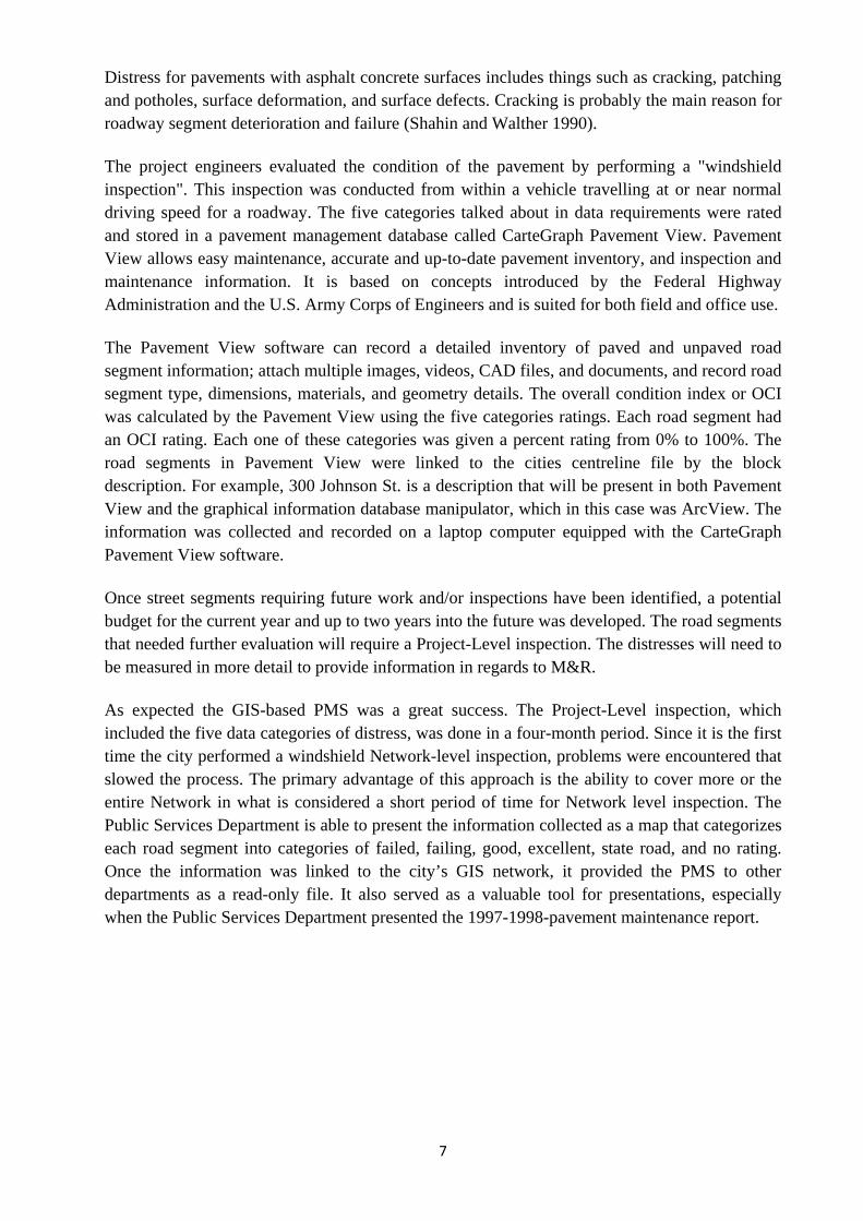
Chapter 3: Abu Dhabi Island Base Map & Geodetic Control Reference For a GIS system to be used as a platform for a pavement management system (PMS) and to be able to enhance the different pavement management processes it should have its two broad classifications of information components very well established, i.e. the spatial data (roads edges, road centre lines & buildings, etc.) and their related attribute data, in short the Base map. Moreover, positional accuracy is an essential factor when it comes to dealing with Linear Referencing Systems (LRS), a very important component in the development of any PMS. Taking these two factors into consideration, it was quite essential to introduce the history and future development of the Base map data used in the course of this research, its source, geodetic reference, positional accuracy and some of the activities done to update the existing database. 3.1 Abu Dhabi Island Base Map Base Mapping for Abu Dhabi Island was done in 1992-1994 by photogrammetric methods within the Interactive Graphic Data Management Systems (IGDMS) project. Aerial photos at a scale of 1:6000 and data were compiled to suit the 1:1250 scale of output, Fig. 1. Positional accuracy for well identified objects (e.g. buildings, road edges, etc.) was maintained at +/- 15 cm. A large number of new attributes were collected from field verification work (especially for buildings) and input to the database during the Base Map Updating Project (1999-2000). For the mainland, existing base map information is created at smaller scales and mostly out-dated (Marcin Kunka 2005).

The last project initiated was the “GIS Data Base Enhancement - DBE” in February 2007. The goal of the project, apart from the new base map for the Mainland, is to update the Base map for Abu Dhabi Island. Data characteristic for the Base map is as shown in Table.1 below,

Figure 1.Software and Base Map sample of Abu Dhabi city - Planning and Surveying Sector, Abu Dhabi Municipality

9

Table 1.Abu Dhabi Emirate Base map characteristics Area Data Type Main Land

(Area B) Abu Dhabi Island

(Area A) Vector Data -Vector base map of accuracy (Std dev)– 0.35m -Vector base map of accuracy (Std dev) – 0.2m

Raster Data

Orthomaps:

-Date of Aerial survey – December & Feb. 2007

-Resolution - 0.20m

Satellite Imagery:

IKONOS – Resolution of 1m, 2-3 times a year

Orthomaps:

-Date of Aerial survey – November 2007

-Resolution - 0.10m

Satellite Imagery:

IKONOS – Resolution of 1m, 2-3 times a year

This can be further illustrated as shown below, Fig. 2.

3.2 Geodetic Control The Abu Dhabi Island control network was created in 1992 for the IGDMS Project and consisted of approximately 450 points, well monumented, surveyed (GPS campaign) and described. It is considered as a 2nd and 3rd order control with accuracy +/- 1 cm. This network is subject to continuous ruin due to extensive construction activity on the Island.

Figure 2.Abu Dhabi Emirate Base map Updating – GIS Database Enhancement Project, December 2007. Spatial Data Directorate – Town Planning Department, GIS Section

10

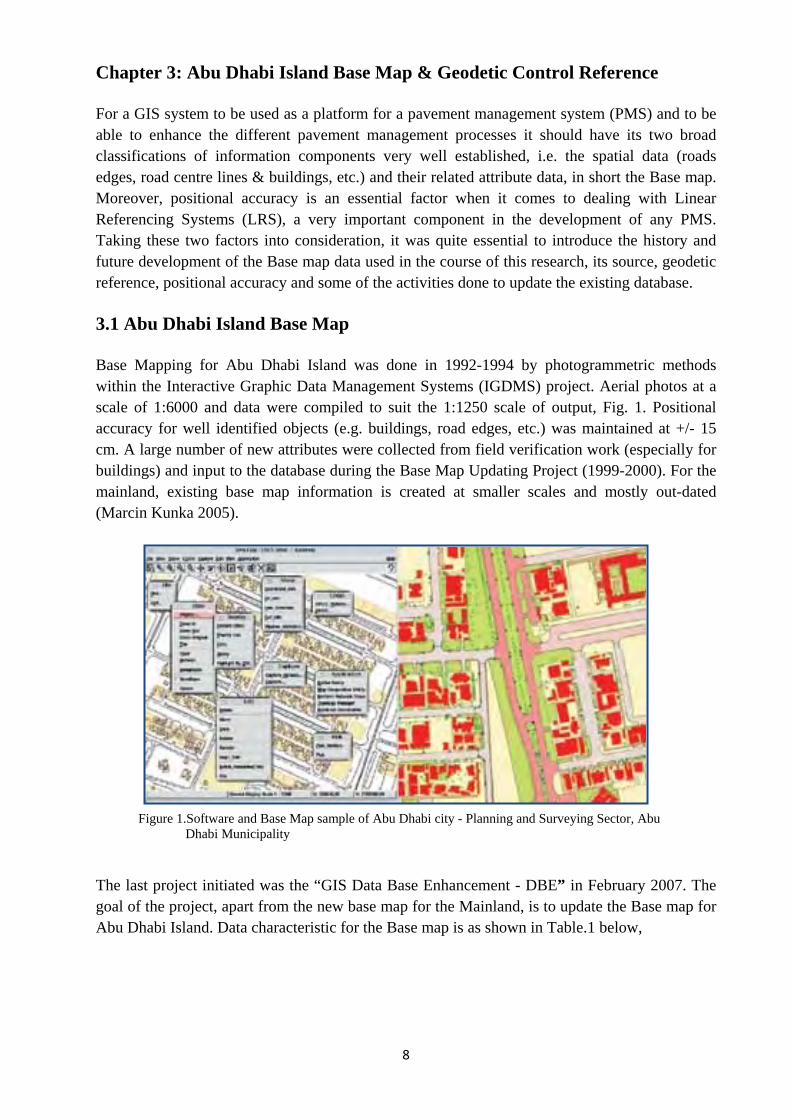
The network was mostly updated and re-established (approx. 35% of points) in 1999 – 2000 The geodetic network was resurveyed (old control) and additional control points were established in 2007. The total number of network Ground Control Points (GCP) is 811. The positional accuracy of the GCPs on Abu Dhabi Island is 0.04 m. The newly constructed GPS Reference Stations Network – GRS, Fig.3 is functioning since November 2007. It provides a positional accuracy of 0.02 – 0.03 m for Real Time Kinematics - RTK observations. The service is available 24 hours a day, seven days per week (Marcin Kunka 2005).

3.2.1 Abu Dhabi Island-Datum The first major geodetic datum of the Arabian Gulf area was established by W.E. Browne of the Iraq Petroleum Company in 1927-1931 at the South End Base at station Nahrwan (East of Baghdad) such that: Fo = 33° 19’ 10.87” North, Lo = +44° 43’ 25.54” East of Greenwich, and the Clarke 1880 is the ellipsoid of reference where: a = 6,378,300.782 m, and 1/f = 293.4663077. The Nahrwan Datum of 1929 is the most prevalent coordinate system of the entire Arabian Gulf area and is still found to this day. In 1967, the Directorate of Military Surveys recomputed the Mainland True Coast and Qatar triangulations on the International Ellipsoid, European Datum 1950. The coordinates were then transformed into Nahrwan Datum 1929 (Mugnier Clifford 2001). 3.2.2 Nahrwan to WGS 84 Datum Transformation The transformation between references frames can be determined by simply performing satellite coordinates observation on points of known position in a particular datum and performing a transformation to a geocentric coordinate system. Hence the geocentric coordinates of a point using both the satellite coordinate system and the datum would be determined. The difference in this pair of geocentric coordinates would represent a shift between the satellite reference system, and the regional reference system.

Figure 2.Distribution of the GPS Reference Station Network

11

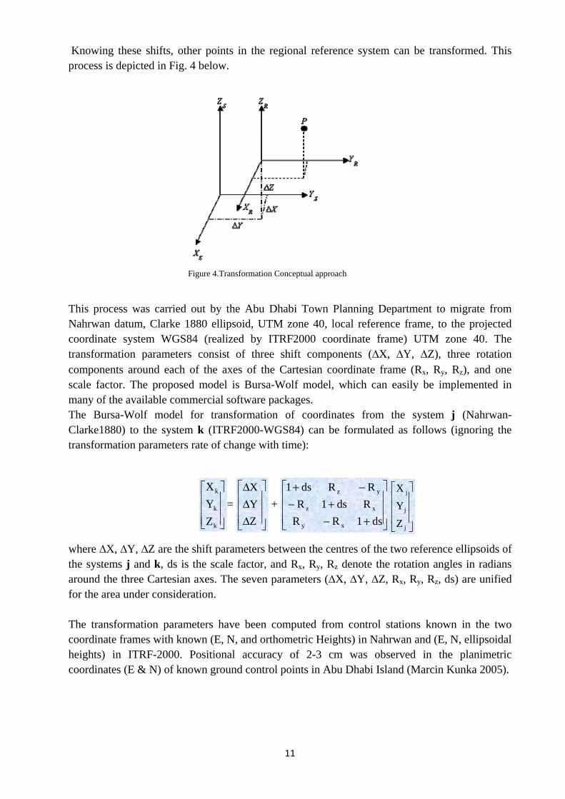
Knowing these shifts, other points in the regional reference system can be transformed. This process is depicted in Fig. 4 below.

This process was carried out by the Abu Dhabi Town Planning Department to migrate from Nahrwan datum, Clarke 1880 ellipsoid, UTM zone 40, local reference frame, to the projected coordinate system WGS84 (realized by ITRF2000 coordinate frame) UTM zone 40. The transformation parameters consist of three shift components (∆X, ΔY, ΔZ), three rotation components around each of the axes of the Cartesian coordinate frame (Rx, Ry, Rz), and one scale factor. The proposed model is Bursa-Wolf model, which can easily be implemented in many of the available commercial software packages. The Bursa-Wolf model for transformation of coordinates from the system j (Nahrwan-Clarke1880) to the system k (ITRF2000-WGS84) can be formulated as follows (ignoring the transformation parameters rate of change with time):

⎥⎥⎥

⎦

⎤

⎢⎢⎢

⎣

⎡

k

k

k

ZYX

= ⎥⎥⎥

⎦

⎤

⎢⎢⎢

⎣

⎡

ΔΔΔ

ZYX

+ ⎥⎥⎥

⎦

⎤

⎢⎢⎢

⎣

⎡

+−+−

−+

ds1RRRds1RRRds1

xy

xz

yz

⎥⎥⎥

⎦

⎤

⎢⎢⎢

⎣

⎡

j

j

j

Z

Y

X

where ∆X, ∆Y, ∆Z are the shift parameters between the centres of the two reference ellipsoids of the systems j and k, ds is the scale factor, and Rx, Ry, Rz denote the rotation angles in radians around the three Cartesian axes. The seven parameters (∆X, ∆Y, ∆Z, Rx, Ry, Rz, ds) are unified for the area under consideration. The transformation parameters have been computed from control stations known in the two coordinate frames with known (E, N, and orthometric Heights) in Nahrwan and (E, N, ellipsoidal heights) in ITRF-2000. Positional accuracy of 2-3 cm was observed in the planimetric coordinates (E & N) of known ground control points in Abu Dhabi Island (Marcin Kunka 2005).

Figure 4.Transformation Conceptual approach

12

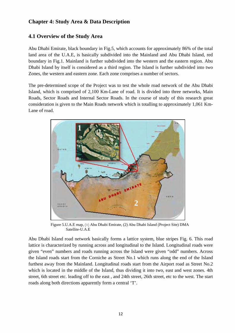
Chapter 4: Study Area & Data Description 4.1 Overview of the Study Area Abu Dhabi Emirate, black boundary in Fig.5, which accounts for approximately 86% of the total land area of the U.A.E, is basically subdivided into the Mainland and Abu Dhabi Island, red boundary in Fig.1. Mainland is further subdivided into the western and the eastern region. Abu Dhabi Island by itself is considered as a third region. The Island is further subdivided into two Zones, the western and eastern zone. Each zone comprises a number of sectors. The pre-determined scope of the Project was to test the whole road network of the Abu Dhabi Island, which is comprised of 2,100 Km-Lane of road. It is divided into three networks, Main Roads, Sector Roads and Internal Sector Roads. In the course of study of this research great consideration is given to the Main Roads network which is totalling to approximately 1,061 Km-Lane of road.

Abu Dhabi Island road network basically forms a lattice system, blue stripes Fig. 6. This road lattice is characterized by running across and longitudinal to the Island. Longitudinal roads were given “even” numbers and roads running across the Island were given “odd” numbers. Across the Island roads start from the Corniche as Street No.1 which runs along the end of the Island furthest away from the Mainland. Longitudinal roads start from the Airport road as Street No.2 which is located in the middle of the Island, thus dividing it into two, east and west zones. 4th street, 6th street etc. leading off to the east , and 24th street, 26th street, etc to the west. The start roads along both directions apparently form a central ‘T’.

Figure 5.U.A.E map, (1) Abu Dhabi Emirate, (2) Abu Dhabi Island (Project Site) DMA Satellite-U.A.E

1

2

13

Figure 6.Abu Dhabi Island main roads network

4.2 Data Description & Acquisition 4.2.1 Roughness & IRI Determination Roughness is defined in accordance with the Standards of the Vehicles-Pavement Systems (ASTM E867) as "The deviation of a surface from a true planar surface with characteristic dimensions that affect vehicle dynamics and ride quality" i.e. it is an expression of irregularities in the pavement surface that adversely affect the ride quality in a vehicle. The World Bank found road roughness to be a primary factor in the analyses and trade-offs involving road quality vs. user cost in terms of vehicle delay costs, fuel consumption and maintenance costs (David W. Moore 1998). It is widely regarded as the most important measure of pavement performance because it is the measure most evident to the travelling public (Appendix E, HPMS Field Manual 2005). Roughness can be quantified by two distinct approaches:

1) Present Serviceability Rating (PSR) 2) International Roughness Index (IRI)

PSR, according to the National Research Council (U.S.) - Highway Research Board, 1962 is defined as "The judgment of an observer as to the current ability of a pavement to serve the traffic it is meant to serve". The AASHTO Road Test (Highway Research Board, 1962) developed this definition for the present serviceability rating. It is based on individual observation. In the course of this project, this method was not implemented and much preference was given to the second approach. 1. International Roughness Index (IRI) The international roughness index (IRI) was developed by the World Bank in the 1980s. IRI is used to define a characteristic of the longitudinal profile of a travelled wheel track and constitutes a standardized roughness measurement. The commonly recommended units are meters per kilometre (m/km) or millimetres per meter (mm/m). The IRI is based on the average rectified slope (ARS), which is a filtered ratio of a standard vehicle's accumulated suspension

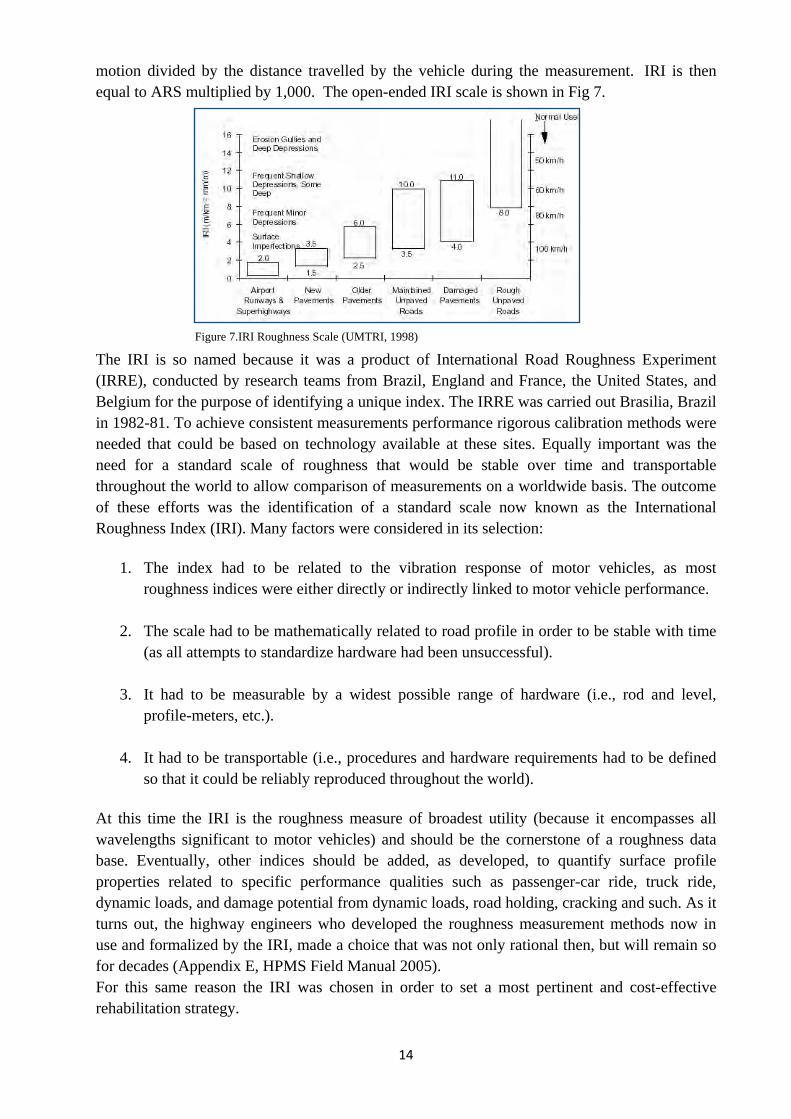
14

motion divided by the distance travelled by the vehicle during the measurement. IRI is then equal to ARS multiplied by 1,000. The open-ended IRI scale is shown in Fig 7.

The IRI is so named because it was a product of International Road Roughness Experiment (IRRE), conducted by research teams from Brazil, England and France, the United States, and Belgium for the purpose of identifying a unique index. The IRRE was carried out Brasilia, Brazil in 1982-81. To achieve consistent measurements performance rigorous calibration methods were needed that could be based on technology available at these sites. Equally important was the need for a standard scale of roughness that would be stable over time and transportable throughout the world to allow comparison of measurements on a worldwide basis. The outcome of these efforts was the identification of a standard scale now known as the International Roughness Index (IRI). Many factors were considered in its selection:

1. The index had to be related to the vibration response of motor vehicles, as most roughness indices were either directly or indirectly linked to motor vehicle performance.

2. The scale had to be mathematically related to road profile in order to be stable with time (as all attempts to standardize hardware had been unsuccessful).

3. It had to be measurable by a widest possible range of hardware (i.e., rod and level,

profile-meters, etc.).

4. It had to be transportable (i.e., procedures and hardware requirements had to be defined so that it could be reliably reproduced throughout the world).

At this time the IRI is the roughness measure of broadest utility (because it encompasses all wavelengths significant to motor vehicles) and should be the cornerstone of a roughness data base. Eventually, other indices should be added, as developed, to quantify surface profile properties related to specific performance qualities such as passenger-car ride, truck ride, dynamic loads, and damage potential from dynamic loads, road holding, cracking and such. As it turns out, the highway engineers who developed the roughness measurement methods now in use and formalized by the IRI, made a choice that was not only rational then, but will remain so for decades (Appendix E, HPMS Field Manual 2005). For this same reason the IRI was chosen in order to set a most pertinent and cost-effective rehabilitation strategy.

Figure 7.IRI Roughness Scale (UMTRI, 1998)

15

2. GPS Measurement The project requirement clearly necessitated the need for acquiring the positions of roughness sampling during the testing. Thus, the latest model of Trimble GPS ProXRS which has a sub cm differential accuracy was employed. The Trimble ProXRS GPS Pathfinder receiver being employed is an integrated satellite differential receiver. The integrated satellite differential capability of GPS Pathfinder ProXRS decodes and uses satellite differential corrections to provide sub-meter position accuracy. Internationally, it is sometimes required to subscribe to a satellite differential correction service. This type of receivers supports the OmniSTAR satellite differential correction service. Since UAE is under the coverage of Integrated Beacons, which are transmitting the differentially corrected signals there was no need for subscribing for a differential correction service. 3. Video logging & Video Survey Video Logging and Video Surveys were carried out for all the road networks within the Abu Dhabi Island using a digital camera Fig.8. Emphasis during the course of the video survey was mainly on:

• To cover overall Carriageway • To cover the Pavement’s Condition • Road Furniture, such as Traffic Signs, Walkways

and Pavement Markings Direct digitizing of the video is accomplished through an IEEE Fire wire connection in the computer. It is common practice during the course of the surveys to sample the images at intervals of 5 – 10 m. In order to get a clear high resolution image and to capture as many road related entities as possible, the video logging was carried out at 5 m intervals. During the Survey, images will be recorded with all data displayed on the PC screen overlaid on the image. The data is digitized directly to the computer. Road Description, speed, Milestones and GPS coordinates were typical type of data that was instantly overlaid on the image during the survey.

Figure 8.Video Camera

16

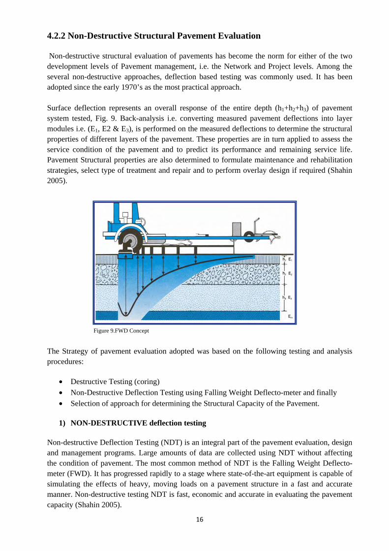
4.2.2 Non-Destructive Structural Pavement Evaluation Non-destructive structural evaluation of pavements has become the norm for either of the two development levels of Pavement management, i.e. the Network and Project levels. Among the several non-destructive approaches, deflection based testing was commonly used. It has been adopted since the early 1970’s as the most practical approach. Surface deflection represents an overall response of the entire depth (h1+h2+h3) of pavement system tested, Fig. 9. Back-analysis i.e. converting measured pavement deflections into layer modules i.e. (E1, E2 & E3), is performed on the measured deflections to determine the structural properties of different layers of the pavement. These properties are in turn applied to assess the service condition of the pavement and to predict its performance and remaining service life. Pavement Structural properties are also determined to formulate maintenance and rehabilitation strategies, select type of treatment and repair and to perform overlay design if required (Shahin 2005).

The Strategy of pavement evaluation adopted was based on the following testing and analysis procedures:

• Destructive Testing (coring) • Non-Destructive Deflection Testing using Falling Weight Deflecto-meter and finally • Selection of approach for determining the Structural Capacity of the Pavement.

1) NON-DESTRUCTIVE deflection testing

Non-destructive Deflection Testing (NDT) is an integral part of the pavement evaluation, design and management programs. Large amounts of data are collected using NDT without affecting the condition of pavement. The most common method of NDT is the Falling Weight Deflecto-meter (FWD). It has progressed rapidly to a stage where state-of-the-art equipment is capable of simulating the effects of heavy, moving loads on a pavement structure in a fast and accurate manner. Non-destructive testing NDT is fast, economic and accurate in evaluating the pavement capacity (Shahin 2005).

Figure 9.FWD Concept

17

2) Deflections Pavement surface deflection measurements are the primary means of evaluating a flexible pavement structure and rigid pavement load transfer. Although other measurements can be made that reflect (to some degree) a pavement's structural condition, surface deflection is an important pavement evaluation method because the magnitude and shape of pavement deflection is a function of traffic (type and volume), pavement structural section, temperature affecting the pavement structure and moisture affecting the pavement structure. Deflection measurements can be used in back-calculation methods to determine pavement structural layer stiffness and the sub-grade resilient modulus. Thus, many characteristics of a flexible pavement can be determined by measuring its deflection in response to load. Furthermore, pavement deflection measurements are non-destructive (AASHTO, 1986).

18

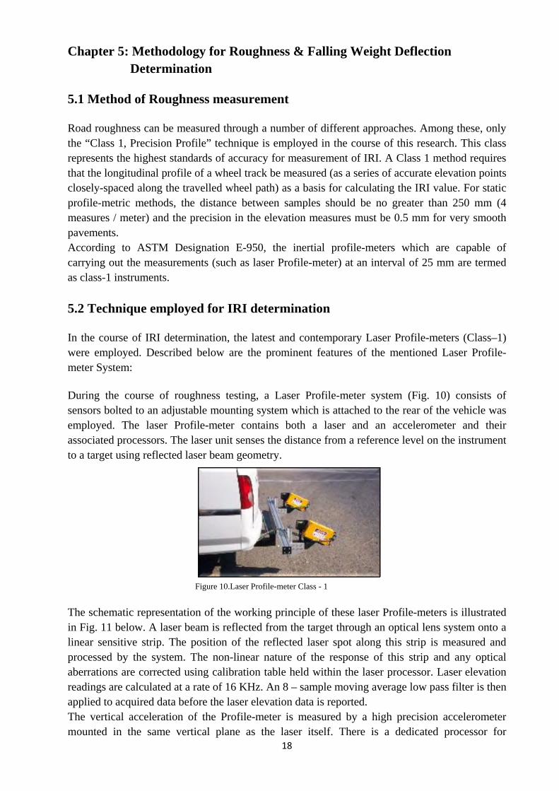
Chapter 5: Methodology for Roughness & Falling Weight Deflection Determination 5.1 Method of Roughness measurement Road roughness can be measured through a number of different approaches. Among these, only the “Class 1, Precision Profile” technique is employed in the course of this research. This class represents the highest standards of accuracy for measurement of IRI. A Class 1 method requires that the longitudinal profile of a wheel track be measured (as a series of accurate elevation points closely-spaced along the travelled wheel path) as a basis for calculating the IRI value. For static profile-metric methods, the distance between samples should be no greater than 250 mm (4 measures / meter) and the precision in the elevation measures must be 0.5 mm for very smooth pavements. According to ASTM Designation E-950, the inertial profile-meters which are capable of carrying out the measurements (such as laser Profile-meter) at an interval of 25 mm are termed as class-1 instruments. 5.2 Technique employed for IRI determination In the course of IRI determination, the latest and contemporary Laser Profile-meters (Class–1) were employed. Described below are the prominent features of the mentioned Laser Profile-meter System: During the course of roughness testing, a Laser Profile-meter system (Fig. 10) consists of sensors bolted to an adjustable mounting system which is attached to the rear of the vehicle was employed. The laser Profile-meter contains both a laser and an accelerometer and their associated processors. The laser unit senses the distance from a reference level on the instrument to a target using reflected laser beam geometry.

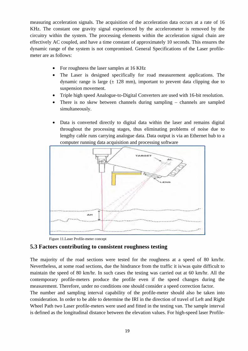
The schematic representation of the working principle of these laser Profile-meters is illustrated in Fig. 11 below. A laser beam is reflected from the target through an optical lens system onto a linear sensitive strip. The position of the reflected laser spot along this strip is measured and processed by the system. The non-linear nature of the response of this strip and any optical aberrations are corrected using calibration table held within the laser processor. Laser elevation readings are calculated at a rate of 16 KHz. An 8 – sample moving average low pass filter is then applied to acquired data before the laser elevation data is reported. The vertical acceleration of the Profile-meter is measured by a high precision accelerometer mounted in the same vertical plane as the laser itself. There is a dedicated processor for

Figure 10.Laser Profile-meter Class - 1

19

measuring acceleration signals. The acquisition of the acceleration data occurs at a rate of 16 KHz. The constant one gravity signal experienced by the accelerometer is removed by the circuitry within the system. The processing elements within the acceleration signal chain are effectively AC coupled, and have a time constant of approximately 10 seconds. This ensures the dynamic range of the system is not compromised. General Specifications of the Laser profile-meter are as follows:

• For roughness the laser samples at 16 KHz • The Laser is designed specifically for road measurement applications. The

dynamic range is large (± 128 mm), important to prevent data clipping due to suspension movement.

• Triple high speed Analogue-to-Digital Converters are used with 16-bit resolution. • There is no skew between channels during sampling – channels are sampled

simultaneously.

• Data is converted directly to digital data within the laser and remains digital throughout the processing stages, thus eliminating problems of noise due to lengthy cable runs carrying analogue data. Data output is via an Ethernet hub to a computer running data acquisition and processing software

5.3 Factors contributing to consistent roughness testing The majority of the road sections were tested for the roughness at a speed of 80 km/hr. Nevertheless, at some road sections, due the hindrance from the traffic it is/was quite difficult to maintain the speed of 80 km/hr. In such cases the testing was carried out at 60 km/hr. All the contemporary profile-meters produce the profile even if the speed changes during the measurement. Therefore, under no conditions one should consider a speed correction factor. The number and sampling interval capability of the profile-meter should also be taken into consideration. In order to be able to determine the IRI in the direction of travel of Left and Right Wheel Path two Laser profile-meters were used and fitted in the testing van. The sample interval is defined as the longitudinal distance between the elevation values. For high-speed laser Profile-

Figure 11.Laser Profile-meter concept

20

meters the interval is the distance travelled by the vehicle between the times the computer “samples” digital readings from the transducers. The laser Profile-meter system “Class – 1” instrument is capable of gathering the data “elevations” at an interval of 25 mm. Classification of the different equipments against their longitudinal sampling criteria is shown in table no.2 below.

Table 2.Equipment Vs Longitudinal Sampling

S.N. Equipment Classification Longitudinal Sampling

1. Class - 1 Less than or equal to 25 mm (1 in)

2. Class - 2 Greater than 25 mm (1 in) to 150 mm (6 in)

3. Class - 3 Greater than 300 mm (12 in)

5.4 Falling Weight Deflection (FWD) Principle, System & Measurement

Technique Several NDT Deflection measuring techniques are adopted for use in pavement evaluation work. In general, non-destructive deflection testing equipment can be categorized into three major groups.

• Static Deflection • Steady State (Sinusoidal) Deflection • Impact load deflections (FWD)

Out of these systems, Impact Devices-‘Falling Weight Deflecto-meter’ is the most popular Deflection Measuring System. FWD testing was carried at 100 m intervals and in the direction of the right wheel path. Testing plans were valid for two, three and four lane dual carriageway. In order to record the deflections at appropriate temperatures and in order to avoid any hindrance and disturbance in the traffic flow FWD testing was carried out at night. 5.4.1 System Overview Two KUAB 2m-FWD machines were used for the evaluation of roads pavement. KUAB - 2m are designed and capable to simulate the actual service load in regard to rate of loading and peak load. This can be performed exactly over a wide range of loads ranging from heavy trucks to large aircraft, Fig. 12.

Figure 12.FWD KUAB-2M machine

21

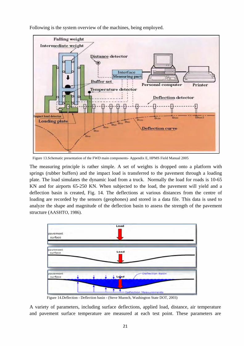
Following is the system overview of the machines, being employed.

The measuring principle is rather simple. A set of weights is dropped onto a platform with springs (rubber buffers) and the impact load is transferred to the pavement through a loading plate. The load simulates the dynamic load from a truck. Normally the load for roads is 10-65 KN and for airports 65-250 KN. When subjected to the load, the pavement will yield and a deflection basin is created, Fig. 14. The deflections at various distances from the centre of loading are recorded by the sensors (geophones) and stored in a data file. This data is used to analyze the shape and magnitude of the deflection basin to assess the strength of the pavement structure (AASHTO, 1986).

A variety of parameters, including surface deflections, applied load, distance, air temperature and pavement surface temperature are measured at each test point. These parameters are

Figure 14.Deflection - Deflection basin - (Steve Muench, Washington State DOT, 2003)

Figure 13.Schematic presentation of the FWD main components- Appendix E, HPMS Field Manual 2005

22

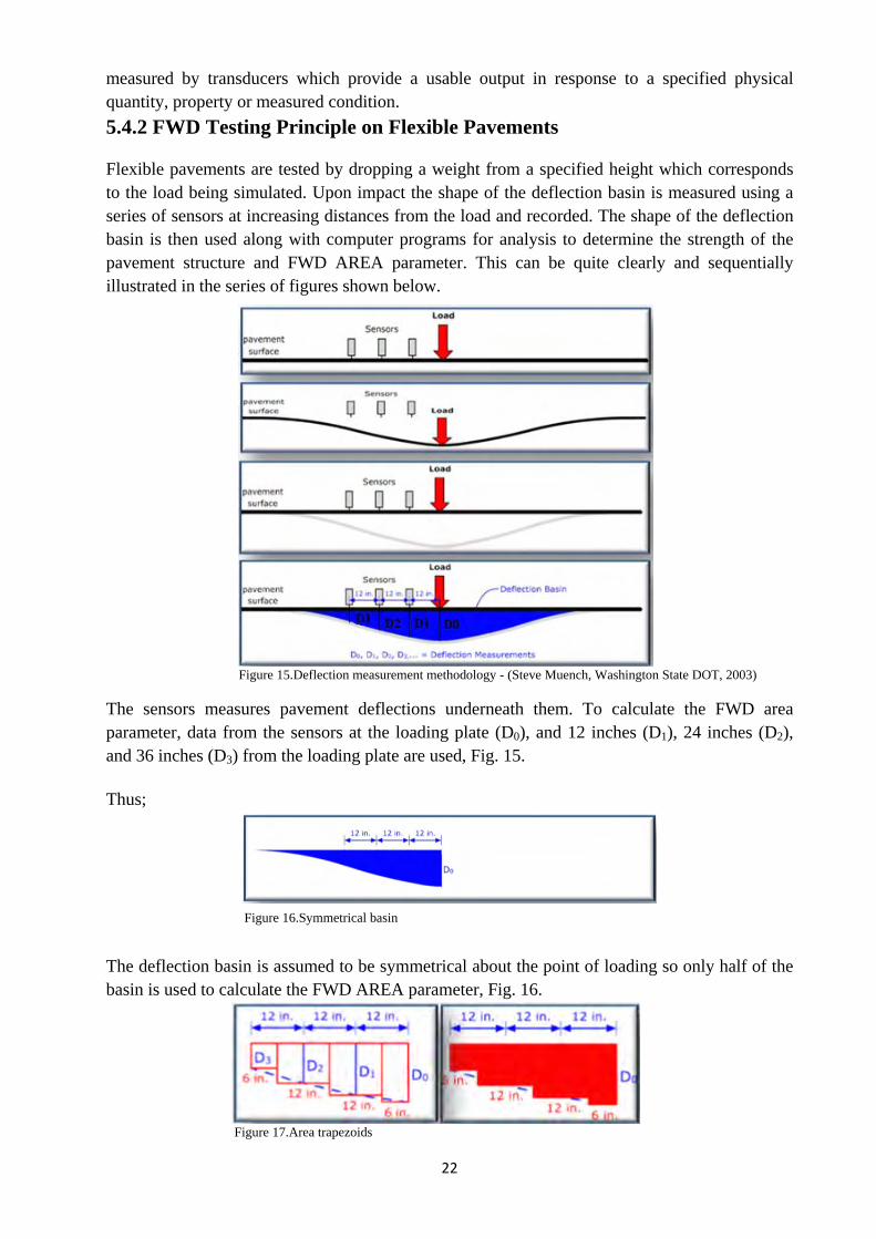
measured by transducers which provide a usable output in response to a specified physical quantity, property or measured condition. 5.4.2 FWD Testing Principle on Flexible Pavements Flexible pavements are tested by dropping a weight from a specified height which corresponds to the load being simulated. Upon impact the shape of the deflection basin is measured using a series of sensors at increasing distances from the load and recorded. The shape of the deflection basin is then used along with computer programs for analysis to determine the strength of the pavement structure and FWD AREA parameter. This can be quite clearly and sequentially illustrated in the series of figures shown below.

The sensors measures pavement deflections underneath them. To calculate the FWD area parameter, data from the sensors at the loading plate (D0), and 12 inches (D1), 24 inches (D2), and 36 inches (D3) from the loading plate are used, Fig. 15. Thus;

The deflection basin is assumed to be symmetrical about the point of loading so only half of the basin is used to calculate the FWD AREA parameter, Fig. 16.

Figure 15.Deflection measurement methodology - (Steve Muench, Washington State DOT, 2003)

Figure 16.Symmetrical basin

Figure 17.Area trapezoids

23

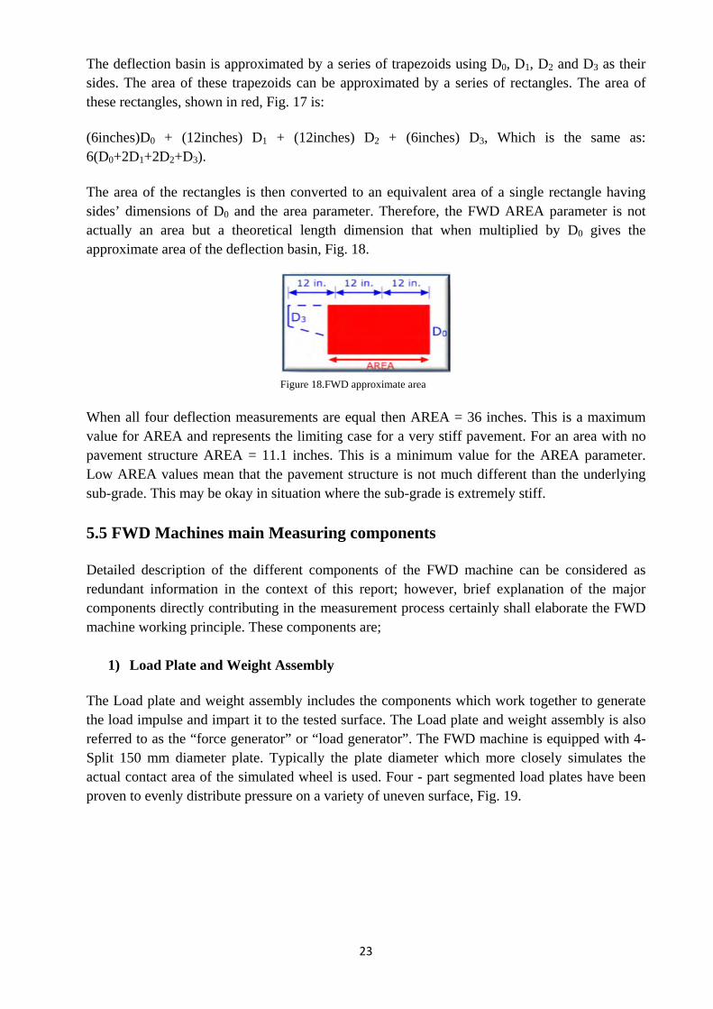
The deflection basin is approximated by a series of trapezoids using D0, D1, D2 and D3 as their sides. The area of these trapezoids can be approximated by a series of rectangles. The area of these rectangles, shown in red, Fig. 17 is: (6inches)D0 + (12inches) D1 + (12inches) D2 + (6inches) D3, Which is the same as: 6(D0+2D1+2D2+D3). The area of the rectangles is then converted to an equivalent area of a single rectangle having sides’ dimensions of D0 and the area parameter. Therefore, the FWD AREA parameter is not actually an area but a theoretical length dimension that when multiplied by D0 gives the approximate area of the deflection basin, Fig. 18.

When all four deflection measurements are equal then AREA = 36 inches. This is a maximum value for AREA and represents the limiting case for a very stiff pavement. For an area with no pavement structure AREA = 11.1 inches. This is a minimum value for the AREA parameter. Low AREA values mean that the pavement structure is not much different than the underlying sub-grade. This may be okay in situation where the sub-grade is extremely stiff. 5.5 FWD Machines main Measuring components Detailed description of the different components of the FWD machine can be considered as redundant information in the context of this report; however, brief explanation of the major components directly contributing in the measurement process certainly shall elaborate the FWD machine working principle. These components are;

1) Load Plate and Weight Assembly The Load plate and weight assembly includes the components which work together to generate the load impulse and impart it to the tested surface. The Load plate and weight assembly is also referred to as the “force generator” or “load generator”. The FWD machine is equipped with 4-Split 150 mm diameter plate. Typically the plate diameter which more closely simulates the actual contact area of the simulated wheel is used. Four - part segmented load plates have been proven to evenly distribute pressure on a variety of uneven surface, Fig. 19.

Figure 18.FWD approximate area

24

2) The load generator unit As indicated by the name KUAB 2-m FWD features two masses i.e. the middle weight and the falling weights. Falling is referred to an assembly (comprising of stake/additional weights) which upon falling at the buffers generate impulse load at the tested surface. Weights can be added or removed from the falling weight and/or middle weight, to change peak load and loading time, Fig. 20.

5.6 Working Principle of the Load Generator The weight assembly comprising of Middle Weight/Falling Weight, Buffer generates a load impulse as follows:

• The plate and the load assembly are lowered to the pavement surface. At this point, the dead weight of the middle weight, foot and load plate is applied to the pavement surface.

• The falling weight is raised to a predetermined height,

depending on the magnitude of the force needed, Fig. 25. Falling weight is released and falls down on a rubber buffer set Fig. 21 on the top of the middle weight. The resulting load transferred through the upper buffers, middle weight. Lower buffers, foot, load plate, rubber plates and finally to the pavement.

Figure 20.Load generator unit

Figure 21.Buffers

Figure 25.Falling Weight

Figure 19.KUAB-2m Load Plate

25

5.7 Structural Capacity Evaluation and Results Interpretation For the purpose of evaluation of existing pavement from the collected deflection data, two approaches are commonly used. These include:

• Pavement Layer Moduli Prediction • Direct Structural Capacity Prediction

Both approaches mentioned above determine the effective structural capacity by making use of the deflections measured by the FWD device. Due to non availability of accurate individual layer thickness data and/or construction or design drawings for the road the first method was not employed for the evaluation of the pavement.

1) Direct Structural Capacity Prediction The second alternative, “Direct Structural Capacity Prediction Technique” is based on the philosophy that the combined stiffness influence of each layer thickness modulus (thickness-layer coefficient) determines overall structural capacity of the pavement. Thus, the maximum deflection obtained from FWD (at the load centre) may be viewed at the result of two separate pavement parameters i.e.

• Structural Capacity • Sub-grade Modulus

This approach recognizes that the structural capacity is a function of the maximum deflection ‘Do’ and sub-grade modulus. Hence, this technique relies on outer deflection values to estimate the sub-grade modulus, and the maximum measured NDT deflection to predict the “effective” structural pavement capacity. While both approaches yield the same result i.e. the same value (effective structural capacity, SCxeff), preferences had been given to the second approach, i.e. direct structural capacity, as it only requires the total pavement thickness and it is independent of the individual layer thickness values. For instance, Layer Moduli Prediction requires thickness of each and every layer of the pavement and such data could only be available, after carrying out the sufficient number of the trial pits (core test). Such operations considering the volume of the traffic were nearly impossible and were not feasible considering the project time frame. Therefore, based on the above stated facts the second approach was adopted for determining the structural capacity of the road pavements.

2) Uniform Pavement Sections This procedure was used in relation to pavement evaluation. It was necessary to divide the pavement into uniform sections. The uniformity is characterized by pavement type, pavement thickness, pavement condition, most importantly the deflections, and sub-grade modulus computed through FWD. Based on these parameters, the pavement has been divided into several uniform sections. For each uniform section, a representative deflection basin has been identified.

26

Deflection values at this location have been used to back-calculate the elasticity modulus of sub-grade, and the effective modulus of the pavement. FWD data was analyzed using “DARWin 3.1”, computer software program for pavement design. DARWin represents the series of AASHTO’s, the American Association of State Highway & Transportation Officials, computer software programs.

3) Representative Deflection Basin (RDB) A representative deflection basin (RDB) was selected for each uniform pavement section based on the statistical analysis of the deflection testing results. For each uniform pavement section, the mean and the standard deviation of the maximum deflection (D0), the existing pavement and field temperature, were determined from the D0 data of the uniform pavement section. The sum of mean plus one standard deviation of D0 was compared to all the D0 values of the Section(s). The station with D0 closest to this sum was selected as the RDB. The final RDBs for all uniform pavement sections are considered in the design and provided in the design Tables. 5.8 Parameters of Evaluation and Design

1) Sub-grade Modulus (Mrsg) AASHTO methodology and design procedures for rehabilitation of existing pavement as outlined in part-III of Guide (AASHTO 93) have been followed for the pavement structural evaluation. According to “1993 AASHTO Guide for the Design of Pavement Structures”, the sub-grade modulus of the existing pavement structure can be predicted by the following relationship.

(1)

Where, P = plate load (lbs) Sr = sub-grade modulus prediction factor, dependents upon the sub-grade Poisson’s

ratio. Dr = pavement surface deflection (in.) measured at r distance, from the load, and r = distance from load to Dr (in.) Mrsg = sub-grade modulus (psi).

2) Effective Pavement Modulus (EP)

Once the Mr of the sub-grade is obtained, the effective pavement modulus, Ep may be derived from the following equation.

(2) Where:

D0 = deflection measured at the centre of the load plate (and adjusted to a standard temperature of 68oF)

p = NDT load plate pressure, psi a = NDT plate radius, in. D = total thickness of pavement layer above the sub-grade, inches Mr = subgrade resilient modulus, psi Ep = effective modulus of all pavement layers above the sub-grade layer, psi.

⎥⎥⎥⎥⎥⎥⎥⎥

⎦

⎤

⎢⎢⎢⎢⎢⎢⎢⎢

⎣

⎡

⎟⎠⎞

⎜⎝⎛+

−

+

+

=p

r

pr

EaD

ME

aDM

paD

2

3

0

1

11

1

15.1

))(())((

rDSPMr

r

rsg =

27

The only unknown in the above equation is the Ep value. The “D0” corresponds to the deflection under the load. Since this deflection is heavily influenced by the asphalt layer, it is important to normalize the deflection at a standard temperature. Because asphalt mix is a temperature sensitive material, its behaviour is heavily influenced by the temperature. At high temperature it behaves like a viscous material, whereas at cold temperatures it is more like an elastic solid. Thus, it is important to evaluate at a common reference temperature. The standard temperature recommended by AASHTO is 68oF. For purposes of comparison of Ep along the length of a project, the measured D0 values should be adjusted to a single reference temperature of 68oF.

3) Effective Structural Number (SN) Making use of the temperature adjusted D0 values and the computed Mr values, “Effective Structural Capacity”, Ep was estimated. The effective modulus Ep was finally used for computing the effective Structural Number (SN) values using equation 3. The relationship used for the computation of SN is given below.

(3) Where “D” = total thickness of the pavement, Once the structural number of the existing pavement is determined, it can be compared with the design structural number of the pavement, which determines the requirement of overlays and vice versa.

4) Required Structural Capacity for Future Traffic, SNf Structural capacity is computed assuming it to be a new pavement. The structural number will be estimated based upon the AASHTO approach. The design is based upon identifying a flexible pavement structure number (SN) to with stand the projected level of axle load traffic. Among the major inputs required for the AASHTO design equation were the design period or duration and the cumulative expected 18-kip equivalent single axle loads (ESALs) during this design period. Since this information was not available, therefore, future traffic (ESALs) was assumed to be 20 million for the design period. Another factor introduced to the design process to incorporate some degree of certainty and to ensure that the design will survive its full life was “Reliability”. For the purpose of this analysis a design reliability of 95 percent was used for establishing the design thickness. The drainage coefficient is also needed to study the impact of presence of water in the unbound base and sub-base layers. This will result in an increase or decrease of the layer thickness depending upon the drainage quality. Given the lack of the appropriate data to estimate the drainage coefficient, a conservative estimate is a value 1.0 for the unbound layers.

30045.0 EpDSN =

28

5) Overall Standard Deviation The value of overall standard deviation (So) in the AASHTO design procedure expresses the possible variation in traffic and material that is going to affect the pavement performance. The AASHTO guide states:

• The estimated overall standard deviation for the case where the variance of the projected future traffic is considered (along with other variance associated with revised pavement performance models) is 0.39 for rigid and 0.49 for flexible pavements.

• The estimated overall standard deviation for the case where the variance of the projected future traffic is not considered (along with other variance associated with revised pavement performance models) is 0.34 for rigid and 0.44 for flexible pavements.

5.9 Determination of Overlay Thickness The Structural number of the existing pavement derived from NDT (SNeff) is compared with the structural number of the newly designed pavement (SNf) in order to suggest if overlay is required or not. For instance if (SNf) is less than the (SNeff) then it is not required to provide any overlay. If (SNeff) is greater than (SNf) then overlay would be required. The thickness of AC overlay over the existing AC pavement can be computed by the following relationship.

(5)

Where:

SNol = required overlay structural number

Aol = structural coefficient of AC overlay

Dol = required overlay thickness, inches

SNf = structure number required to accommodate future traffic

SNeff = effective structural number or effective structural capacity of existing pavement

ol

efff

ol

olol a

SNSNa

SND−

==

29

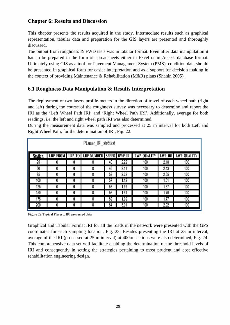
Chapter 6: Results and Discussion This chapter presents the results acquired in the study. Intermediate results such as graphical representation, tabular data and preparation for the GIS layers are presented and thoroughly discussed. The output from roughness & FWD tests was in tabular format. Even after data manipulation it had to be prepared in the form of spreadsheets either in Excel or in Access database format. Ultimately using GIS as a tool for Pavement Management System (PMS), condition data should be presented in graphical form for easier interpretation and as a support for decision making in the context of providing Maintenance & Rehabilitation (M&R) plans (Shahin 2005). 6.1 Roughness Data Manipulation & Results Interpretation The deployment of two lasers profile-meters in the direction of travel of each wheel path (right and left) during the course of the roughness survey was necessary to determine and report the IRI as the ‘Left Wheel Path IRI’ and ‘Right Wheel Path IRI’. Additionally, average for both readings, i.e. the left and right wheel path IRI was also determined. During the measurement data was sampled and processed at 25 m interval for both Left and Right Wheel Path, for the determination of IRI, Fig. 22.

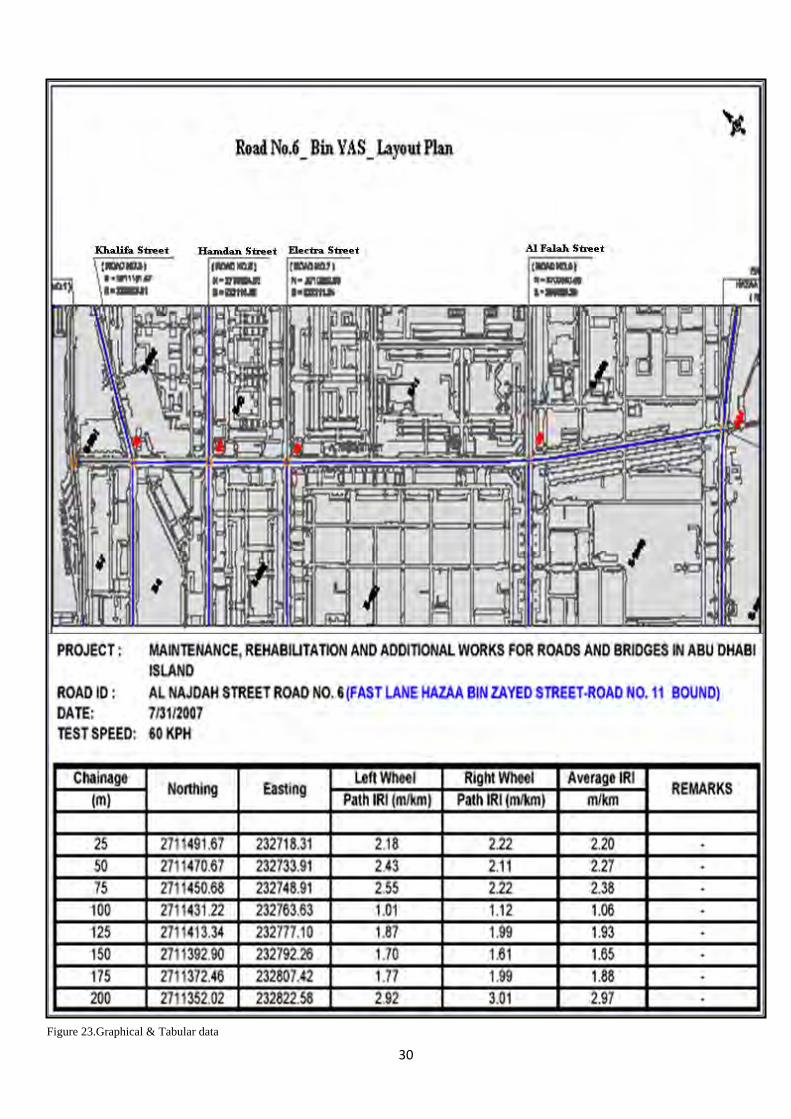
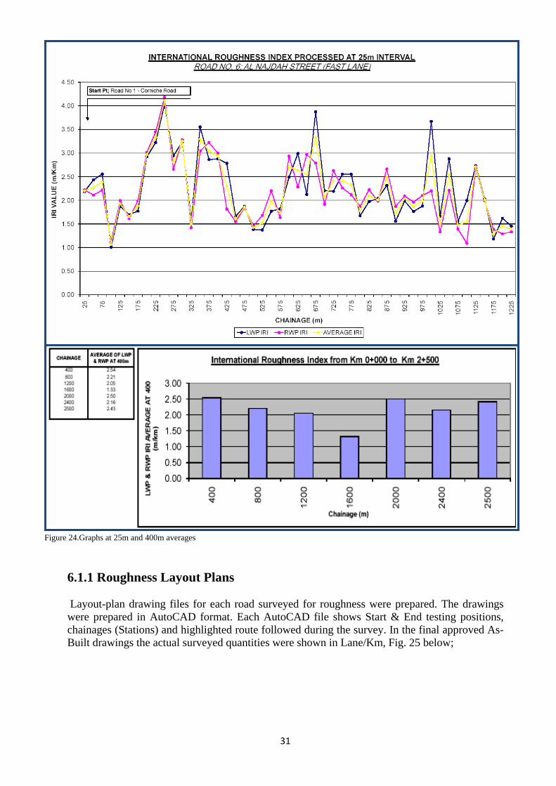
Graphical and Tabular Format IRI for all the roads in the network were presented with the GPS coordinates for each sampling location, Fig. 23. Besides presenting the IRI at 25 m interval, average of the IRI (processed at 25 m interval) at 400m sections were also determined, Fig. 24. This comprehensive data set will facilitate enabling the determination of the threshold levels of IRI and consequently in setting the strategies pertaining to most prudent and cost effective rehabilitation engineering design.

Figure 22.Typical Plaser _ IRI processed data

30

Figure 23.Graphical & Tabular data

31

6.1.1 Roughness Layout Plans Layout-plan drawing files for each road surveyed for roughness were prepared. The drawings were prepared in AutoCAD format. Each AutoCAD file shows Start & End testing positions, chainages (Stations) and highlighted route followed during the survey. In the final approved As-Built drawings the actual surveyed quantities were shown in Lane/Km, Fig. 25 below;

Figure 24.Graphs at 25m and 400m averages

32

6.1.2 IRI GIS-Based Graphical Representation In order to be able to produce GIS maps isolating road sections requiring immediate attention roughness tabular data showing the testing location GPS coordinates as Easting & Northing as well as the average IRI were required. These were the interesting data to be reflected in roughness maps. The IRI classification was based on a certain criterion which determines a range of IRI values for each class. It is worth mentioning here that at this step a supporting criterion for reclassification was received from the Abu Dhabi Road Asset Management & Information System (ADRAMIS). However, it was not applicable to the range of values in the roughness data as the range starts from the value 4.0 with its corresponding 85th percentile speed while the posted speed limit in Abu Dhabi Island mostly is of the value 60Km/h. In other words, the range of classification values was beyond the highest roughness IRI value in our surveyed data. Therefore, another roughness - IRI framework had to be considered. In accordance with the range of IRI, i.e. surveyed data available special consideration was given to another roughness framework as shown in Fig. 26. The scale ranges from Very Good to Very Poor for the corresponding IRI range from less than 1.11 to greater than 3.5 respectively (Michael G. & Richard Scott, 2004).

Figure 25.Graphical layout for road no.06

33

The scale was adapted to the range of IRI attribute values designated to the road lanes and were symbolized accordingly giving a range of five classes. Tabular data for each surveyed road was input into the GIS software ArcGIS 9.2 using the GPS coordinates (Add X, Y data). Thus, surveyed roughness locations were displayed every 25m. It was only showing point features locations but does not give any indication about the surveyed road lane sections. Linear features had to be constructed to resemble the road lanes. By doing so, lines parallel to the road centerline were constructed. Based on the length of the road these line features were segmented according to the number of roughness test taken during the survey. Thus, if there were 250 GPS locations, the corresponding line feature would be divided into 250 segments. These features had no attributes at this stage. Two methods were followed for linear feature representation:

• Join Data by Spatial Location • Direct copy attributes from GPS (X,Y) to corresponding Line segment

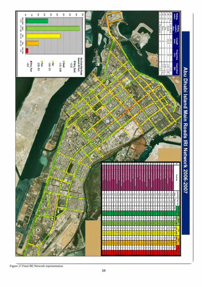
The first method was adopted first. Spatially joining the attribute tables of the GPS coordinates to the segmented line features. Road portions existing in down town areas where high rise buildings hindered satellite signal reception did not have complete GPS locations. Missing (X, Y) coordinates were then interpolated in AutoCAD. As a result, GPS locations inputted into GIS were not following the exact route. The GPS accuracy also was a factor having some of the GPS points shifted away from the lane centerline. In some areas traffic obliged the survey vehicle to deviate from the lane overtaking or undertaking the front vehicle to maintain the speed needed for the survey. All these factors, affected the accuracy of joining the segmented portions to their corresponding IRI values. In the second method, which was finally agreed upon to be adopted, all attributes were directly copied field by field to the attribute table of the lane line features, bearing in mind the direction of survey and the sequence in which the survey was performed, i.e. the fast lane first, the middle lane second and finally the slow lane depending on the direction of the road. Based on the above classification criteria all the roughness results were reclassified and re-tabulated based on the IRI scale for the determination of the new categorized road section ranging from the Very Good section to the Very Poor sections for each road. Thus the overall statistical data for the whole road network in terms of main roads network percentage and roughness measurements final quantities were determined, Fig. 27

Figure 26.IRI classification criteria

34

Figure 27.Final IRI Network representation

35

6.2 FWD Data Manipulation & Results Interpretation

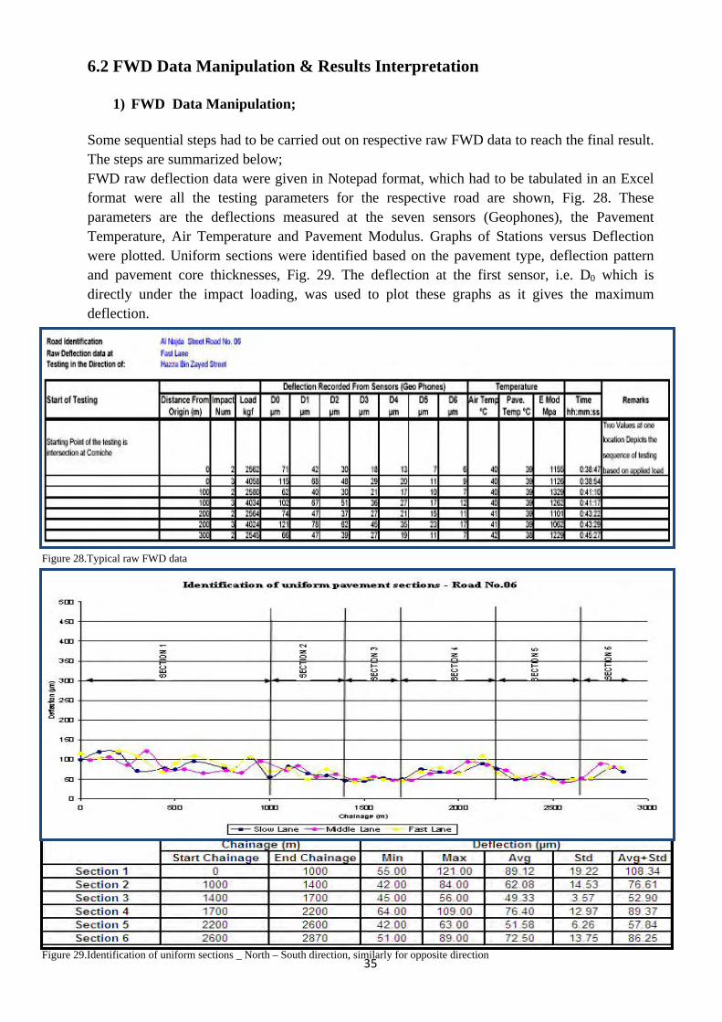
1) FWD Data Manipulation; Some sequential steps had to be carried out on respective raw FWD data to reach the final result. The steps are summarized below; FWD raw deflection data were given in Notepad format, which had to be tabulated in an Excel format were all the testing parameters for the respective road are shown, Fig. 28. These parameters are the deflections measured at the seven sensors (Geophones), the Pavement Temperature, Air Temperature and Pavement Modulus. Graphs of Stations versus Deflection were plotted. Uniform sections were identified based on the pavement type, deflection pattern and pavement core thicknesses, Fig. 29. The deflection at the first sensor, i.e. D0 which is directly under the impact loading, was used to plot these graphs as it gives the maximum deflection.

Figure 28.Typical raw FWD data

Figure 29.Identification of uniform sections _ North – South direction, similarly for opposite direction

36

For each uniform section, a representative deflection basin has been identified, see Section (5.4.1). Deflection values at this location have been used to back-calculate the elasticity modulus of the sub-grade, and the effective modulus of the pavement. Details for the uniform sections were also shown as in Table 3 below. Tabular results were also shown for the determination of the final overlay thicknesses, Table 4. For detailed information please refer to section (5.4.2).

Table 3.Details of Uniform Pavement Sections

S.NO. SECTIONS DEFLECTIONS (mm)

RDB SUBGRADE EFFECTIVE EFFECTIVE

SECTION STD AVERAGE LOCATION DEF MODULUDS1 PAVEMENT EXISTING

AVERAGE +STD MODULUS 2 PAVEMENT

M - M (m) (mm) (psi) (psi) SN

From Road No 1 to Road No 9

1 000 -1000 89.12 19.22 108.34 100 119 26662 302164 7.13 2 1000 -1400 62.08 14.53 76.61 1100 82 18987 805492 8.34

3 1400 -1700 49.33 3.57 52.90 1600 53 26852 1546039 9.32

4 1700 - 2200 76.40 12.97 89.37 2050 94 26754 421577 8.06

5 2200 - 2600 51.58 6.26 57.84 2400 59 23531 1157648 11.15

6 2600 – 2870 72.50 13.75 86.25 2800 80 21384 777609 8.65

From Road No 9 to Road No 1

1 2870-2670 72.56 12.58 85.14 2770 82 21337 646566 8.52 2 2670-2170 55.67 10.71 66.38 2170 69 23069 1118490 8.83

3 2170-1770 69.33 10.17 79.51 2070 82 25430 616495 9.15

4 1770-1470 52.00 5.07 57.07 1470 54 36214 987665 10.26

5 1470-470 66.48 11.23 77.71 870 82 24490 583073 8.87

6 470-000 104.46 18.44 122.90 270 128 25088 288893 7.11

1. Sub-grade Modulus as calculated by DARWin based on AASHTO Guide 1993, applying C factor 0.33 2. Effective Pavement Modulus over Sub-grade

Table 4.Details of Overlay

S.NO. SECTION ASSUMED DESIGN EFFECTIVE ASPHALTIC TRAFFIC SN 1 EXISTING OVERLAY

MILLION PAVEMENT THICKNESS 3

m - m ESALs SN 2 (cm.)

From Road No 1 to Road No 19

1 0 – 1000 20.00 3.73 7.13 No overlay required 2 1000 – 1400 20.00 4.22 8.34 No overlay required

3 1400-1700 20.00 3.72 9.32 No overlay required

4 1700-2200 20.00 3.72 8.06 No overlay required

5 2200-2600 20.00 3.90 11.15 No overlay required

6 2600-2870 20.00 4.04 8.65 No overlay required

From Road No 19 to Road No 1

1 2870-2670 20.00 4.05 8.52 No overlay required 2 2670-2170 20.00 3.93 8.83 No overlay required

3 2170-1770 20.00 3.79 9.15 No overlay required

4 1770-1470 20.00 3.32 10.26 No overlay required

5 1470-470 20.00 3.85 8.87 No overlay required

6 470-000 20.00 3.81 7.11 No overlay required

37

Final quantities pertaining to the FWD testing were reported lane by lane in both directions increment and decrement with respect to the Start point. Finally, the total quantities for each road and for all the roads were recorded. 6.2.1 FWD Layout Plans Layout-plans were similarly prepared for each road surveyed for FWD testing positions. The drawings were prepared in AutoCAD format. Each AutoCAD file shows the Start & End testing positions, chainages (Stations) and highlighted route followed during the survey. In addition, a typical testing plan valid for 3-Lane Dual carriage way is also shown in the Layout plan. Final actual quantities pertaining to the FWD number of testing location surveyed are shown in the final As-Built drawings, Fig. 30.

Figure 30.Final As Built drawing _ Road No.06

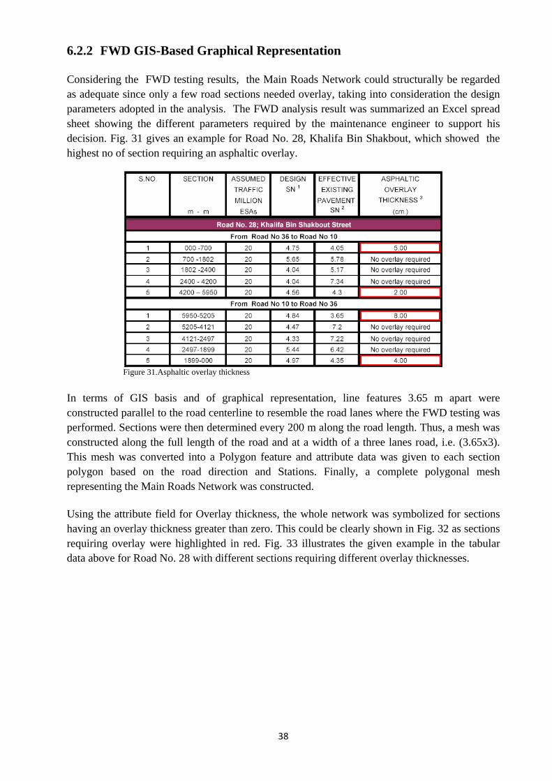
38

6.2.2 FWD GIS-Based Graphical Representation Considering the FWD testing results, the Main Roads Network could structurally be regarded as adequate since only a few road sections needed overlay, taking into consideration the design parameters adopted in the analysis. The FWD analysis result was summarized an Excel spread sheet showing the different parameters required by the maintenance engineer to support his decision. Fig. 31 gives an example for Road No. 28, Khalifa Bin Shakbout, which showed the highest no of section requiring an asphaltic overlay.

In terms of GIS basis and of graphical representation, line features 3.65 m apart were constructed parallel to the road centerline to resemble the road lanes where the FWD testing was performed. Sections were then determined every 200 m along the road length. Thus, a mesh was constructed along the full length of the road and at a width of a three lanes road, i.e. (3.65x3). This mesh was converted into a Polygon feature and attribute data was given to each section polygon based on the road direction and Stations. Finally, a complete polygonal mesh representing the Main Roads Network was constructed. Using the attribute field for Overlay thickness, the whole network was symbolized for sections having an overlay thickness greater than zero. This could be clearly shown in Fig. 32 as sections requiring overlay were highlighted in red. Fig. 33 illustrates the given example in the tabular data above for Road No. 28 with different sections requiring different overlay thicknesses.

Figure 31.Asphaltic overlay thickness

39

Figure 32: FWD Network Plan

Figure 33.FWD Plan _ Road No.28

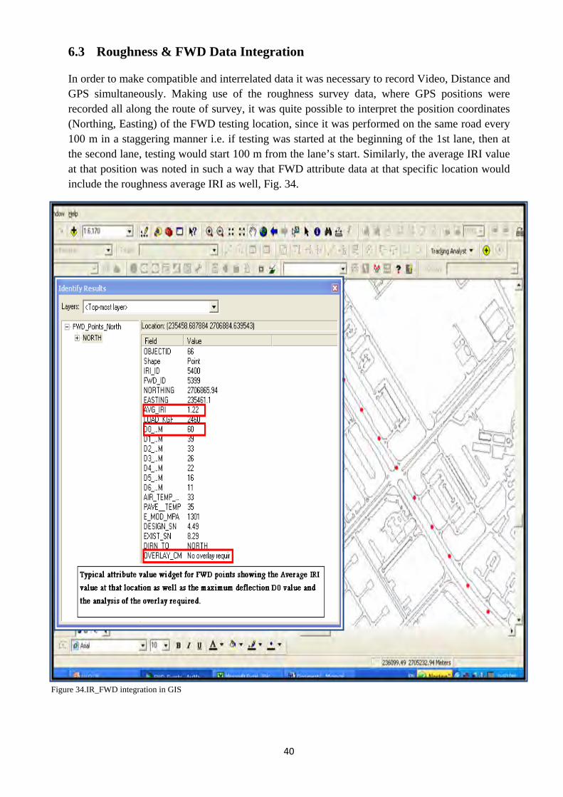
40

6.3 Roughness & FWD Data Integration In order to make compatible and interrelated data it was necessary to record Video, Distance and GPS simultaneously. Making use of the roughness survey data, where GPS positions were recorded all along the route of survey, it was quite possible to interpret the position coordinates (Northing, Easting) of the FWD testing location, since it was performed on the same road every 100 m in a staggering manner i.e. if testing was started at the beginning of the 1st lane, then at the second lane, testing would start 100 m from the lane’s start. Similarly, the average IRI value at that position was noted in such a way that FWD attribute data at that specific location would include the roughness average IRI as well, Fig. 34.

Figure 34.IR_FWD integration in GIS

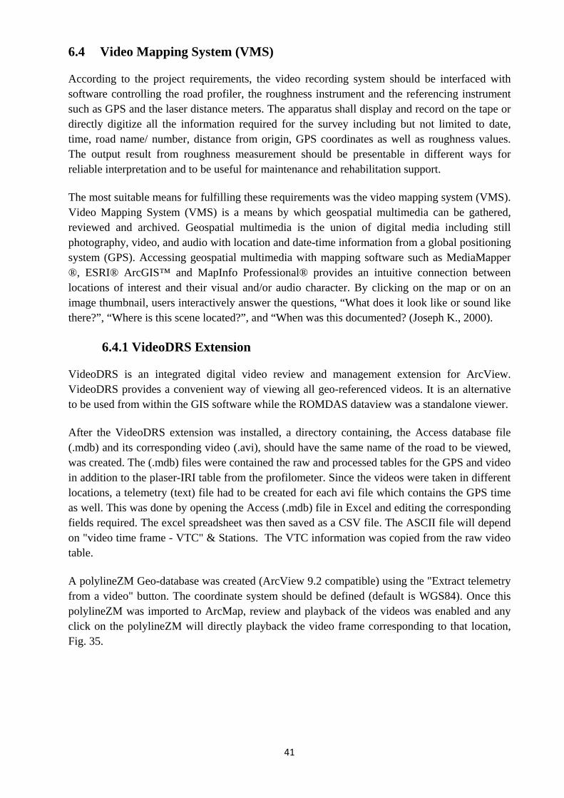
41

6.4 Video Mapping System (VMS) According to the project requirements, the video recording system should be interfaced with software controlling the road profiler, the roughness instrument and the referencing instrument such as GPS and the laser distance meters. The apparatus shall display and record on the tape or directly digitize all the information required for the survey including but not limited to date, time, road name/ number, distance from origin, GPS coordinates as well as roughness values. The output result from roughness measurement should be presentable in different ways for reliable interpretation and to be useful for maintenance and rehabilitation support. The most suitable means for fulfilling these requirements was the video mapping system (VMS). Video Mapping System (VMS) is a means by which geospatial multimedia can be gathered, reviewed and archived. Geospatial multimedia is the union of digital media including still photography, video, and audio with location and date-time information from a global positioning system (GPS). Accessing geospatial multimedia with mapping software such as MediaMapper ®, ESRI® ArcGIS™ and MapInfo Professional® provides an intuitive connection between locations of interest and their visual and/or audio character. By clicking on the map or on an image thumbnail, users interactively answer the questions, “What does it look like or sound like there?”, “Where is this scene located?”, and “When was this documented? (Joseph K., 2000).

6.4.1 VideoDRS Extension VideoDRS is an integrated digital video review and management extension for ArcView. VideoDRS provides a convenient way of viewing all geo-referenced videos. It is an alternative to be used from within the GIS software while the ROMDAS dataview was a standalone viewer. After the VideoDRS extension was installed, a directory containing, the Access database file (.mdb) and its corresponding video (.avi), should have the same name of the road to be viewed, was created. The (.mdb) files were contained the raw and processed tables for the GPS and video in addition to the plaser-IRI table from the profilometer. Since the videos were taken in different locations, a telemetry (text) file had to be created for each avi file which contains the GPS time as well. This was done by opening the Access (.mdb) file in Excel and editing the corresponding fields required. The excel spreadsheet was then saved as a CSV file. The ASCII file will depend on "video time frame - VTC" & Stations. The VTC information was copied from the raw video table. A polylineZM Geo-database was created (ArcView 9.2 compatible) using the "Extract telemetry from a video" button. The coordinate system should be defined (default is WGS84). Once this polylineZM was imported to ArcMap, review and playback of the videos was enabled and any click on the polylineZM will directly playback the video frame corresponding to that location, Fig. 35.

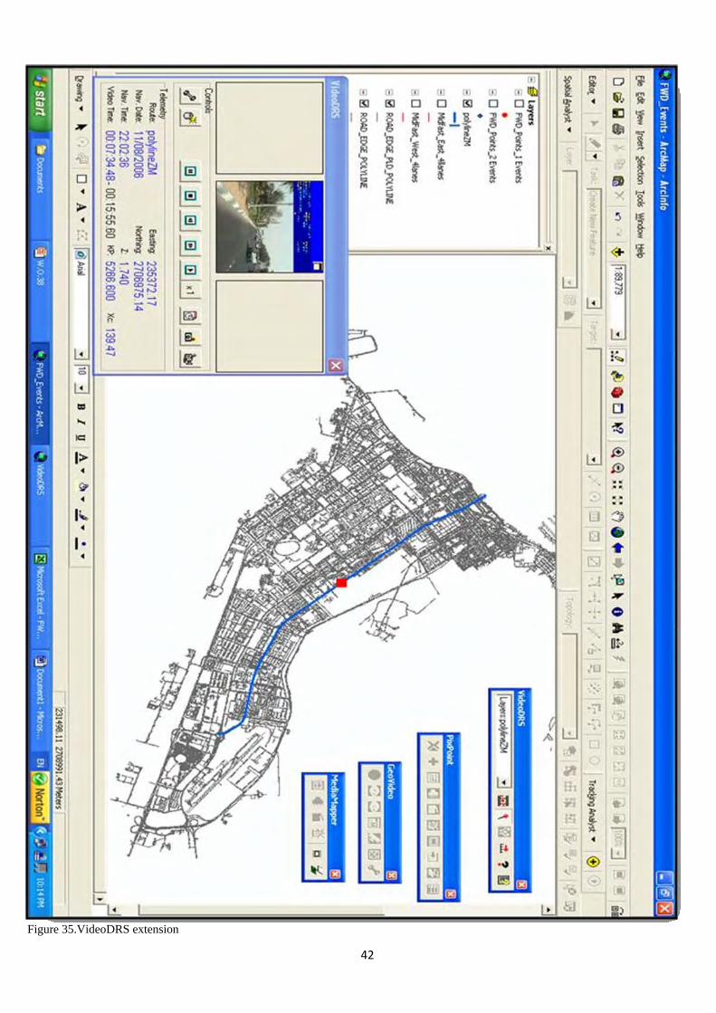
42

Figure 35.VideoDRS extension

43

Another advantage of using this extension was the ability to capture any features observed along the video survey route and create a separate point – geo-database for captured features. This facility was used to collect Road Sign features from the video files to assist in making a road sign inventory. This database was then used to be compared to the collected locations for road signs through site survey using conventional handheld GPS “JUNOst” from Trimble, Fig.36. It worth mentioning here that GIS was also used to create a complete database for some road features in the context of Asset Management, such as Bus-Shelters and Road-Signs.

Figure 36.Road Signs inventory

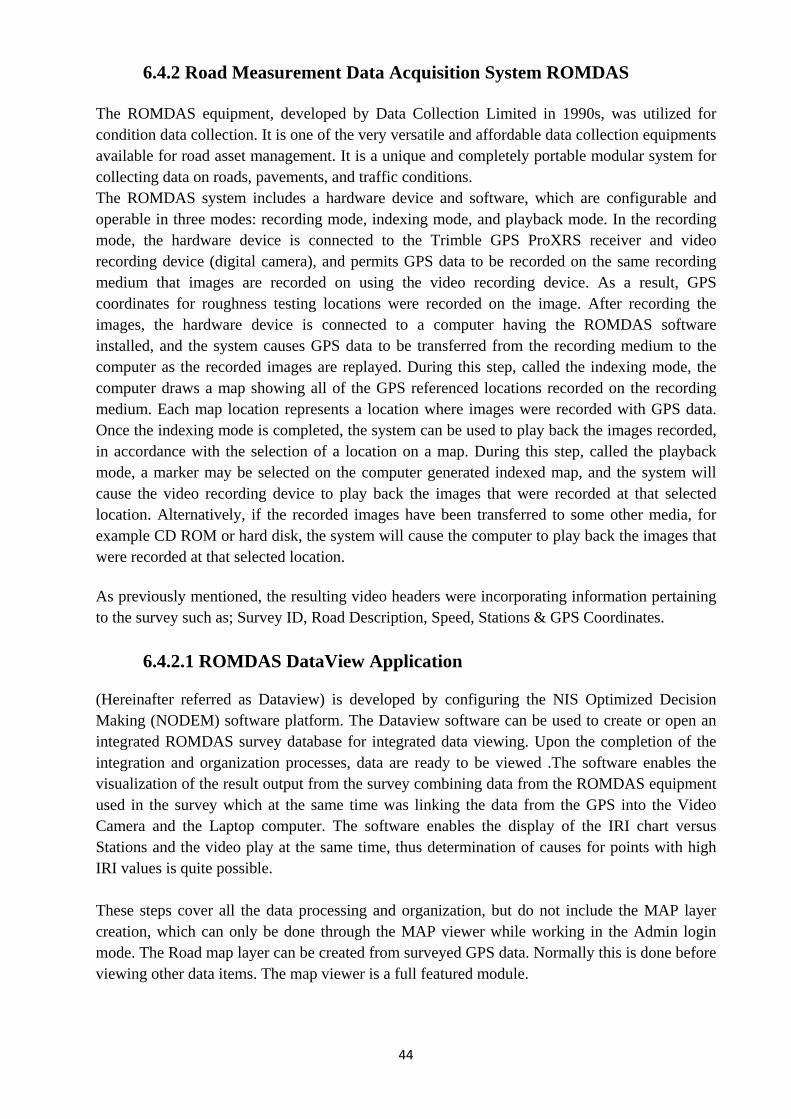
44

6.4.2 Road Measurement Data Acquisition System ROMDAS The ROMDAS equipment, developed by Data Collection Limited in 1990s, was utilized for condition data collection. It is one of the very versatile and affordable data collection equipments available for road asset management. It is a unique and completely portable modular system for collecting data on roads, pavements, and traffic conditions. The ROMDAS system includes a hardware device and software, which are configurable and operable in three modes: recording mode, indexing mode, and playback mode. In the recording mode, the hardware device is connected to the Trimble GPS ProXRS receiver and video recording device (digital camera), and permits GPS data to be recorded on the same recording medium that images are recorded on using the video recording device. As a result, GPS coordinates for roughness testing locations were recorded on the image. After recording the images, the hardware device is connected to a computer having the ROMDAS software installed, and the system causes GPS data to be transferred from the recording medium to the computer as the recorded images are replayed. During this step, called the indexing mode, the computer draws a map showing all of the GPS referenced locations recorded on the recording medium. Each map location represents a location where images were recorded with GPS data. Once the indexing mode is completed, the system can be used to play back the images recorded, in accordance with the selection of a location on a map. During this step, called the playback mode, a marker may be selected on the computer generated indexed map, and the system will cause the video recording device to play back the images that were recorded at that selected location. Alternatively, if the recorded images have been transferred to some other media, for example CD ROM or hard disk, the system will cause the computer to play back the images that were recorded at that selected location. As previously mentioned, the resulting video headers were incorporating information pertaining to the survey such as; Survey ID, Road Description, Speed, Stations & GPS Coordinates.

6.4.2.1 ROMDAS DataView Application (Hereinafter referred as Dataview) is developed by configuring the NIS Optimized Decision Making (NODEM) software platform. The Dataview software can be used to create or open an integrated ROMDAS survey database for integrated data viewing. Upon the completion of the integration and organization processes, data are ready to be viewed .The software enables the visualization of the result output from the survey combining data from the ROMDAS equipment used in the survey which at the same time was linking the data from the GPS into the Video Camera and the Laptop computer. The software enables the display of the IRI chart versus Stations and the video play at the same time, thus determination of causes for points with high IRI values is quite possible. These steps cover all the data processing and organization, but do not include the MAP layer creation, which can only be done through the MAP viewer while working in the Admin login mode. The Road map layer can be created from surveyed GPS data. Normally this is done before viewing other data items. The map viewer is a full featured module.

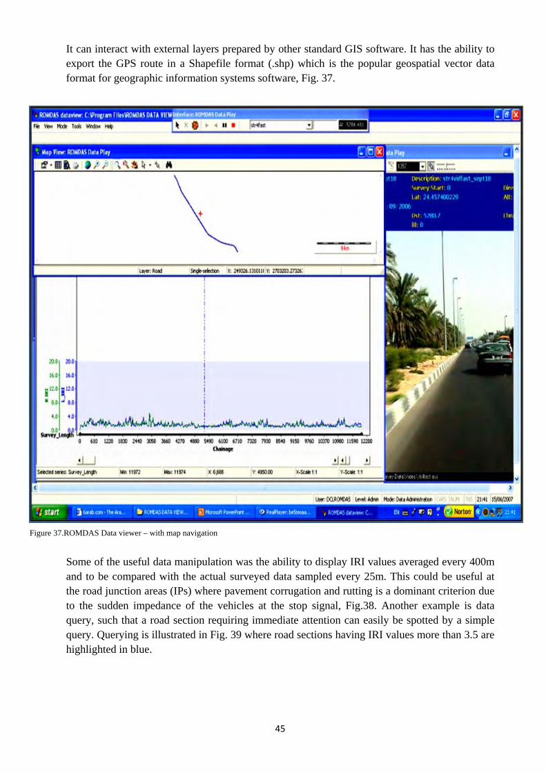
45

It can interact with external layers prepared by other standard GIS software. It has the ability to export the GPS route in a Shapefile format (.shp) which is the popular geospatial vector data format for geographic information systems software, Fig. 37.

Some of the useful data manipulation was the ability to display IRI values averaged every 400m and to be compared with the actual surveyed data sampled every 25m. This could be useful at the road junction areas (IPs) where pavement corrugation and rutting is a dominant criterion due to the sudden impedance of the vehicles at the stop signal, Fig.38. Another example is data query, such that a road section requiring immediate attention can easily be spotted by a simple query. Querying is illustrated in Fig. 39 where road sections having IRI values more than 3.5 are highlighted in blue.

Figure 37.ROMDAS Data viewer – with map navigation

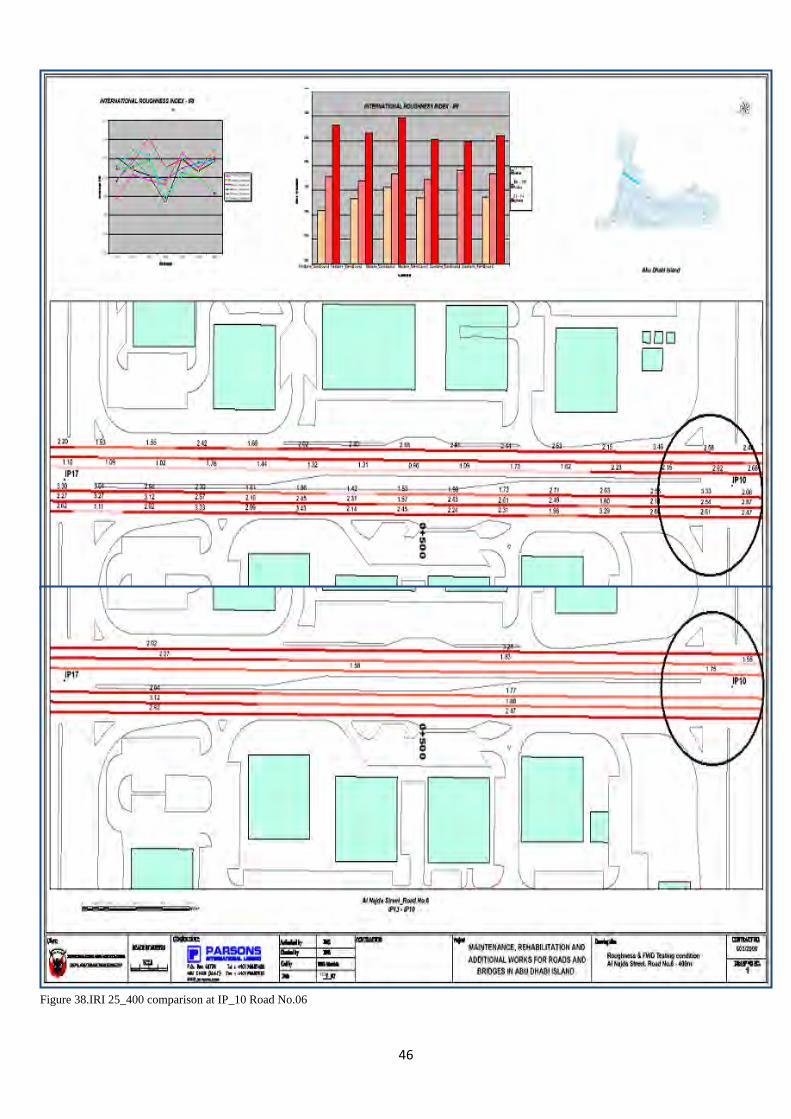
46

Figure 38.IRI 25_400 comparison at IP_10 Road No.06

47

Figure 39.Road Sections with IRI values > 3.5

48

Chapter 7: Conclusion & Recommendations

7.1 Conclusion Direct conclusions can be drawn from the achieved analytical results for both tests roughness and FWD. These can be categorized into two; numerical and theoretical.

1) Numerically, the general condition of the Main Roads Network in terms of ride quality can be regarded as adequate since out of only 2.10 % of the total number of sections is classified as (Very Poor). (Poor) sections are classified as 10.24 % only. A jump of 27.52 % for the (Fair) sections and the majority of the sections are classifies as (Good) with a percentage of 42.41 while the (Very Good) sections are classified as 17.72 % Fig. 40.

CATEGORIES TOTAL

SECTION/CATEGORY

TOTAL NO

SECTIONS PERCENTAGE

VERY GOOD 4811 27145 17.72%

GOOD 11513 27145 42.41%

FAIR 7470 27145 27.52%

POOR 2781 27145 10.24%

VERY POOR 570 27145 2.10%

Figure 40.IRI categories and classification – Final result

2) An average value over 400 m section doesn’t significantly reflect the actual condition of

the road section as the high IRI values mingle with the lower IRI values. Thus, an intermediate IRI value is noted instead concealing the original status of the pavement surface.

3) In terms of the structural adequacy of the Island’s Main Roads Network only 3.5% of the

sections would need milling and overlay treatment according to the depths (cm). The rest of the network exhibits very good existing structural condition and requires no overlay even for a future traffic of 20 million ESALs.

49

7.2 Recommendations The pavement condition of the main roads network was analyzed by making use of data obtained from field studies such as roughness, FWD testing, coring operation, coarse visual condition survey and other data. Some of the major observations and recommendation made are discussed below:

• At the intersections (IPs), another filter less than 25 meters should be considered for the calculations of IRI, presumably 10 meters or even 5 meters. This shorter wavelength will show the defective/extremely corrugated sections at the intersection areas of the road network.

• According to Ministry of Public Work and Housing’s (Federal Government of UAE) and Road and Transport Authority (Government of Dubai) Guidelines/Specifications, The ride ability of the finished wearing course when tested with a Laser Road Surface Testing Machine shall have an IRI (International Roughness Index) not exceeding an average value over a 400m section <1 whereas peak value over a 25 meter section < 1.5 m/km (not more than 2 values per 400meters). Under the circumstance it is recommended to use hot recycling technique to renovate and refurbish the pavement and bring it to the high standards adopted in the United Arab Emirates.

• The spatial nature of transportation data makes GIS a logical choice on which to base

systems such as PMS. GIS has proved to be an effective tool for integrating, managing, storing, displaying, mapping, querying, and spatially analyzing transportation data.

• A GIS-based PMS provides an efficient means for identifying empirical patterns and relationships that might not be detected using standard statistical and descriptive methods.

• Graphical display of data trends is an effective method of communication between the

system and user.

• The GIS-PMS also serve as a sophisticated Asset Management System since GIS with its spatial capabilities can resembles the geographical nature of assets such as pavement networks, utility network and road furniture such as Road Traffic Signs, Bus Stops Sheds and so on.

• PMS should be considered a tool for decision making, not a decision maker in and of

itself. These systems are not intended to replace engineering expertise and judgment, but rather to help in making cost-effective decisions. The system should be flexible enough to incorporate user input in the decision making process.

50

7.3 Future Work preparation According to “Abu Dhabi Road Asset Management Information System, “ADRAMIS” project officials, roughness is not the only parameter that is taken into consideration to develop and implement a Pavement Management System. In fact, structural capacity parameters (FWD), visual parameters, maintenance history and others are also considered to contribute in the development of a Decision Process and a comprehensive maintenance program At this stage, the only two components taken into consideration were roughness and FWD. Other component such as Pavement Condition Index PCI is in the process or at the survey stage. Future completion processes include but not limited to:

1) Completion of the whole roads database with all the types of surveys recorded i.e. all distresses, construction & maintenance history and so on.

2) Synchronization between visualization and the tabular attribute data to be maintained.

3) GIS/PMS integration to be accomplished using the ArcSDE geo-database technology and Microsoft’s SQL Server database.

4) Maintenance & Rehabilitation scenarios or applications to be developed.

5) Finally, a web site should be developed and deployed in the Client’s Premises or Offices

using ArcIMS web application to ensure managerial level access to the latest pavement distress maps and budgeting scenarios.

51

References

AASHTO, 1986 "Guide for Design of Pavement Structures", AASHTO, Washington D.C.

Berry Joseph K. 2000; two part series “Beyond Mapping”, GEOWorld online issues for September and October (Vol. 13, NO. 9-10)

Bham Ghulam H., Nasir G. Gharaibeh and Michael I. Darter, July 2001 “Development of GIS-Based Illinois Highway Pavement Management System” - ESRI User Conference, San Diego, California

David W. Moore, June 1998 “Roughness” Report No.UMTRI-98-2, University of Michigan Transportation Research Institute, Michigan, U.S.A.

Farallon Geographic INC. 2005, Case Study: “GIS PavePlan Application Helps San Mateo County Manage Pavement Conditions”. http://www.fargeo.com/press/releases/gis-paveplan-application-helps-san-mateo-county-manage-pavement-conditions.htm Gillespie Thomas D., 1992 “Everything about IRI”, the University of Michigan Transportation Research Institute, Road profile user group meeting Lincoln, Nebraska

Jain Neelam, and P. K. Nanda, 2003 “Geographical Information System for Pavement Management Systems”, Development.net, Map Asia conference, India

Kunka Marcin, M. Polak, Balaji K. & M. Abou-Seif, 2005 “Municipal GIS, The Abu Dhabi experience”, Map Middle East, U.A.E.

Michael G. and Richard Scott, 2004, Adapting pavement evaluation methodology to the performance based contract of the Fredericton-Moncton Highway Project (A Public-Private Partnership)”, Annual Conference of the Transportation Association of Canada Québec City, Québec - Canada

MUGNIER CLIFFORD J., C.P., C.M.S, 2001 “Grids and Datum of the United Arab Emirates”, ASPRS, U.S.A

Parida M., 2005 “Enhancing pavement management systems using GIS”, Transport 158, Issue TR2, Rookee, India

R. Haas and W.R. Hudson. 1978 "Pavement Management Systems", McGraw-Hill, Inc., New York, N.Y.

Saunders Jeff, June 12, 2005“Real-time Pavement Management”, Farallon Geographics, Directions Magazine, U.S.A

SHAHIN M.Y. and J.A. Walther, 1990 "Pavement Maintenance Management for Roads and Streets Using the PAVER System", USACERL Technical Report M-90/05, Washington D.C

SHAHIN M.Y. 2005 “Pavement Management for Airports, Roads, and Parking Lots” – Second Edition

U.S Department of Transportation – Federal Highway Administration, 2005 “Measuring Pavement Roughness” - Appendix E, Highway Performance Monitoring System Field Manual. Appendix E Measuring Pavement Roughness - HPMS Field Manual_IRI.mht

Weber Lena, and Pat Rooney, 2002 “Albany International Airport, New York, Uses GIS for Pavement Management” ESRI News, U. S. A

Zimmerman Kathryn A., 1997 “Taking Pavement Management into the Next Millennium”, National Workshop on Pavement Management, U.S.A

Reports in Geographic Information Technology 2006-2009 The TRITA-GIT Series - ISSN 1653-5227

2006 06-001 Uliana Danila. Corrective surface for GPS-levelling in Moldova. Master of Science thesis in geodesy

No. 3089. Supervisor: Lars Sjöberg. TRITA-GIT EX 06-001. January 2006. 06-002 Ingemar Lewén. Use of gyrotheodolite in underground control network. Master of Science thesis in

geodesy No. 3090. Supervisor: Erick Asenjo. TRITA-GIT EX 06-002. January 2006. 06-003 Johan Tornberg. Felfortplantningsanalys i GIS-projekt genom Monte Carlo-simulering. Master of

Science thesis in geoinformatics. Supervisor: Mats Dunkars. TRITA-GIT EX 06-003. February 2006. 06-004 Constantin-Octavian Andrei. 3D affine coordinate transformations. Master of Science thesis in

geodesy No. 3091. Supervisor: Huaan Fan. TRITA-GIT EX 06-004. March 2006. 06-005 Helena von Malmborg. Jämförelse av Epos och nätverks-DGPS. Master of Science thesis in geodesy

No. 3092. Supervisor: Milan Horemuz. TRITA-GIT EX 06-005. March 2006. 06-006 Lina Ståhl. Uppskattning av kloridhalt i brunnar - modellering och visualisering med hjälp av SAS-

Bridge. Master of Science thesis in geoinformatics. Supervisor: Hans Hauska. TRITA-GIT EX 06-006. May 2006.

06-007 Dimitrios Chrysafinos. VRS network design considerations applicable to the topology of the Hellenic

Positioning System (HEPOS) stations. Master of Science thesis in geodesy No.3093. Supervisor: Lars Sjöberg. TRITA-GIT EX 06-007. May 2006.

06-008 Tao Zhang. Application of GIS and CARE-W systems on water distribution networks. Master of

Science thesis in geoinformatics. Supervisor: Mats Dunkars. TRITA-GIT EX 06-008. May 2006. 06-009 Krishnasamy Satish Kumar. Usability engineering for Utö tourism information system. Master of

Science thesis in geoinformatics. Supervisor: Mats Dunkars. TRITA-GIT EX 06-009. May 2006. 06-010 Irene Rangle. High resolution satellite data for mapping Landuse/land-cover in the rural-urban fringe

of the Greater Toronto area. Supervisor: Yifang Ban. TRITA-GIT EX 06-010. May 2006. 06-011 Kazi Ishtiak Ahmed. ENVISAT ASAR for land-cover mapping and change detection. Supervisor:

Yifang Ban. TRITA-GIT EX 06-011. May 2006. 06-012 Jian Liang. Synergy of ENVISAT ASAR and MERIS data for landuse/land-cover classification.

Supervisor: Yifang Ban. TRITA-GIT EX 06-012. May 2006. 06-013 Assad Shah. Systematiska effecter inom Riksavvägningen. Master of Science thesis in geodesy

No.3094. Supervisor: Tomas Egeltoft. TRITA-GIT EX 06-013. August 2006. 06-014 Erik Trehn. GPS Precise Point Positioning – An Investigation In Reachable Accuracy. Master of

Science thesis in geodesy No.3095. Supervisor: Milan Horemuz. TRITA-GIT EX 06-014. August 2006.

2007 07-001 Carl Schedlich. Turn at the roundabout: A practical assessment of spatial representations in two

different GPS interfaces from a pedestrian’s perspective. Bachelor of Science thesis in geoinformatics. Supervisor: Michael Le Duc. January 2007.

07-002 Staffan Bengtsson. Förändringsanalys i ortofoton. Master of Science thesis in geoinformatics.

Supervisor: Jonas Nelson and Patric Jansson. TRITA-GIT EX 07-002. March 2007. 07-003 Joseph Addai. Qantification of temporal changes in metal loads – Moss data over 20 years. Master of

Science thesis in geoinformatics. Supervisor: Katrin Grunfeld. March 2007. 07-004 Stephen Rosewarne. Deformation study of the Vasa Ship. Bachelor of Science thesis in geodesy

No.3097. Suppervisor: Milan Horemuz. March 2007. 07-005 Naeim Dastgir. Processing SAR Data Using Range Doppler and Chirp Scaling Algorithms. Master of

Science thesis in geodesy No.3096. Supervisor: Lars Sjöberg. April 2007. 07-006 Torgny Israelsson and Youssef Shoumar. Motion Detection with GPS. Master of Science thesis in

geodesy No.3098. Supervisor: Milan Horemuz. April 2007. 07-007 Akjol Djenaliev. Multicriteria decision making and GIS for railroad planning in Kyrgyzstan. Master of

Science thesis in geoinformatics. Supervisor: Hans Hauska. May 2007. 07-008 Anna Hammar. Quality comparison of automatic 3D city house modelling methods from laser data.

Master of Science thesis in geodesy No.3099. Supervisor: Milan Horemuz. May 2007. 07-009 Md Ubydul Haque. Mapping malaria vector habitats in the dry season in Bangladesh using Spot

imagery. Master of Science thesis in geoinformatics. Supervisor: Hans Hauska. May 2007. 07-010 Jing Jiang. Analysis of the Suitable and Low-Cost Sites for Industrial Land Using Multi Criteria

Evaluation: A Case of Panzhihua, China. Master of Science thesis in geoinformatics. Supervisor: Yifang Ban. June 2007.

07-011 Raghavendra Jayamangal. Quantification of coastal erosion along Spey Bay and the Spey River using

photogrammetry and LiDAR imagery-derived DTMs. Master of Science thesis in geoinformatics. Supervisor: Yifang Ban and Jim Hansom. June 2007.

07-012 Alicia E. Porcar Lahoz. An analysis of how geographical factors affect real estate prices. Master of

Science thesis in geoinformatics. Supervisor: Yifang Ban. October 2007. 07-013 Ebenezer Kwakye Bentum. Detection of land use change in the Accra Metropolitan Area from 1990

to 2000. Master of Science thesis in geoinformatics. Supervisor: Hans Hauska. November 2007.

07-014 Jesper Gradin. Aided inertial navigation field tests using an RLG IMU. Master of Science thesis in geodesy No.3100. Supervisor: Milan Horemuz. December 2007.

2008 08-001 Wan Wen. Road Roughness Detection by analyzing IMU Data. Master of Science thesis in

geodesy No.3101. Supervisor: Milan Horemuz. Janaury 2008.

08-002 Ilias Daras. Determination of a gravimetric geoid model of Greece using the method of KTH. Master of Science thesis in geodesy No.3102. Supervisor: Huaan Fan and Kalliopi Papazissi. Janaury 2008.

08-003 Anwar Negash Surur. Surveying, modelling and visualisation of geological structures in the

Tunberget tunnel. Master of Science thesis in geoinformatics. Supervisor: Hans Hauska. February 2008.

08-004 Helena Swanh. Noggrannhetskontroll av data 3D-modell från pulsskanner och fasmätningsskanner. Master of Science thesis in geodesy No.3103. Supervisor: Milan Horemuz. March 2008.

08-005 Henrik Löfqvist. Inpassning av mätdata i inhomogena nät. Master of Science thesis in geodesy

No.3104. Supervisor: Milan Horemuz and Anders Viden. April 2008. 08-006 Cement Takyi. Lineament study in the Björkö area using satellite radar and airborne VLF data -

possible tools for groundwater prospecting. Master of Science thesis in geoinformatics. Supervisor: Herbert Henkel. June 2008.

08-007 Qarin Bånkestad. 3D data: Faktisk hantering för att kunna lagra, återfå och visualisera tredimensionell

information. Master of Science thesis in geoinformatics. Supervisor: Hans Hauska. June 2008. 08-008 Tadesse Tafesse Kebede. Development and implementation of filter algorithms and controllers to a

construction machine simulator. Master of Science thesis in geodesy No.3105. Supervisor: Lars Sjöberg. September 2008.

08-009 Gulilat Tegane Alemu. Assessments of effects on mixing different types of GPS antennas and

receivers. Master of Science thesis in geodesy No.3106. Supervisor: Lars Sjöberg. September 2008. 08-010 Jure Kop. Tests of New Solutions to the Direct and Indirect Geodetic Problems on the Ellipsoid.

Master of Science thesis in geodesy No.3107. Supervisor: Lars Sjöberg. September 2008. 08-011 Karoliina Kolehmainen. Monitoring and Analysis of Urban Land Cover Changes over Stockholm

Region between 1986 and 2004 using Remote Sensing and Spatial Metrics. Master of Science thesis in geoinformatics. Supervisor: Yifang Ban. October 2008.

08-012 Johan Wallin. Land-Cover Mapping in Stockholm Using Fusion of ALOS PALSAR and SPOT Data.

Master of Science thesis in geoinformatics. Supervisor: Yifang Ban. October 2008. 08-013 Mårten Korall. A comparison between GNSS, Laser scanning and Photogrammetry for volume

calculation of aggregates and gravel materials. Master of Science thesis in geodesy No.3108. Supervisor: Milan Horemuz. December 2008.

2009 09-001 Ahmed Abdallah. Determination of a gravimetric geoid if Sudan using the KTH method.

Master ofScience thesis in geodesy No.3109. Supervisor: Huaan Fan. Janaury 2009. 09-002 Hussein Mohammed Ahmed Elhadi. GIS, a tool for pavement management. Master of

Science thesis in geoinformatics. Supervisor: Hans Hauska. February 2009.

TRITA-GIT EX 09-02

ISSN 1653-5227

ISRN KTH/GIT/EX--09/002-SE