GIS in Air Pollution Research, the Role of Building Surfaces

Stephen C. Hurlock, Jochen StutzDepartment of Atmospheric and Oceanic SciencesUniversity of California, Los Angelessteveh@atmos.ucla.edu

Paper 20422004 ESRI International User Conference

San Diego, CaliforniaAugust 11, 2004

GIS in Air Pollution Research, the Role of Building Surfaces

Stephen C. Hurlock, Jochen Stutz, Department of Atmospheric and Oceanic SciencesUniversity of California, Los Angelessteveh@atmos.ucla.edu

ABSTRACTBuildings can strongly influence air quality because their surfaces chemically process gases, such as nitrogen oxides, and their volumes affect pollutant concentrations. However, actual surface areas and volumes and their vertical distributions are thus far poorly characterized, limiting our ability to model this important aspect of urban air pollution.This paper presents the first application of GIS to quantify the distribution of surface areas and volumes for use in urban air quality models. GIS data from the city of Santa Monica was used to develop 3-D models of selected areas, representative of various urban environments. These models allow calculation of factors such as building surface area, building volume and open air volume. Inclusion of these factors into new and evolving air quality models shows striking results and should lead to higher fidelity calculations of the vertical and temporal distributions of pollutants in urban environments.

“Comparing the air of cities to the air of deserts and arid landsis like comparing waters that are befouled and turbid to waters that are fine and pure. In the city, because of the height of its buildings, the narrowness of its streets, and all that pours forth from its inhabitants and their superfluities…the air becomes stagnant, turbid, thick, misty, and foggy… .”

The influence of buildings on urban air quality has been recognized for a long time.

Quoted in: Barbara J. Finlayson-Pitts, James N. Pitts, Jr., “Chemistry of the Upper and Lower Atmosphere,” 2000, Academic Press

Moses Maimonides, Hebrew philosopher, scientist, and jurist, 1135-1204, wrote:

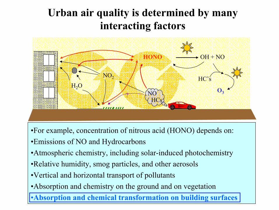
Urban air quality is determined by many interacting factors

NO

NO2

H2O?

HONO OH + NO

HC’s

O3

•For example, concentration of nitrous acid (HONO) depends on:•Emissions of NO and Hydrocarbons•Atmospheric chemistry, including solar-induced photochemistry•Relative humidity, smog particles, and other aerosols•Vertical and horizontal transport of pollutants•Absorption and chemistry on the ground and on vegetation•Absorption and chemical transformation on building surfaces

HCs

Optical absorption measurements show time-dependent vertical profiles of pollutant concentrations

Height: Light path:DOAS ~140 mADEQ ~110 m Upper ~3.51 km × 2Hilton ~ 45 m Middle ~3.29 km × 2MLT ~ 10 m Lower ~3.23 km × 2

6/16/2001 21:00 6/17/2001 00:00 6/17/2001 03:00 6/17/2001 06:000

20406080

Local Time

NO

2 (pp

b)

01

23

HO

NO

(ppb

) 05

1015

HC

HO

(ppb

)

020406080

100

Ox (

ppb)

0

20

40

60

O3 (

ppb)

050

100150200250

Upper Box Middle Box Lower Box

NO

3 (pp

t)

~ 3.5 kmWang, S., R. Ackermann, A. Geyer, J. C. Doran, W. J. Shaw, J. D. Fast, C. W. Spicer, and J. Stutz, Vertical Variation of Nocturnal NOx, Chemistry in the Urban Environment of Phoenix, Proc. 83rd AMS Ann., 2003

Observations can be plotted as vertical concentration profiles

6/16/2001 21:00 6/17/2001 00:00 6/17/2001 03:00 6/17/2001 06:000

20406080

Local Time

NO

2 (pp

b)

01

2

3

HO

NO

(ppb

) 0

5

10

15

HC

HO

(ppb

)

020406080

100

Ox (

ppb)

0

20

40

60

O3 (

ppb)

050

100150200250

Upper Box Middle Box Lower Box

NO

3 (pp

t)

0.0 0.3 0.6 0.9 1.2 1.50

20

40

60

80

100

120

140

Hei

ght (

m)

HONO (ppb)0 50 100 150 200

0

20

40

60

80

100

120

140

NO3 (ppt)

0 10 20 30 40 500

20

40

60

80

100

120

140

Hei

ght (

m)

NO2 (ppb)0 10 20 30 40

0

20

40

60

80

100

120

140

O3 (ppb)

Derived profiles at 00:19am 6/17/2001Phoenix

Direct measurements throughout the night, 6/16-17/2001

Phoenix

Profiles in this height vs. concentration form can be compared with model calculations

Chemical transport models confirm observed concentration profiles

Building volumes and surfaces have not been previously included in urban atmospheric chemistry models.

0 10 20 30 40 50 600

20

40

60

80

100 B

O3 [ppb]

0 5 10 15 20 250

20

40

60

80

100 C

NO2 [ppb]

0 1 2 3 4 5 60

20

40

60

80

100 A

Altit

ude

[m]

Alti

tude

[m]

NO [ppb]

Altit

ude

[m]

0 5 10 15 20 250

20

40

60

80

100 E

NO3 [ppt]

0 100 200 300 4000

20

40

60

80

100 F

N2O5 [ppt]

20 40 60 80 1000

20

40

60

80

100 D after 1h after 2h after 3h after 4h after 5h after 6h

α-pinene [ppt]

Geyer, A., and J. Stutz, Vertical Profiles of NO3, N2O5, O3, andNOx in the Nocturnal Boundary Layer: 2. Model studies on the altitude dependence of composition and chemistry, J. GeophysRes., vol. 109, doi:10.1029/2003JD004211, 2004

How do buildings influence urban air quality?

•Building surfaces process pollutant gases•Absorption, chemical transformation and release•Depends on surface area or surface/volume vs. height•These parameters and functions are not available and not currently included in air quality models

•Buildings occupy volume, resulting in increased pollutant concentrations•e.g., traffic emissions in an urban canyon•Building volumes vs. height are not available and not currently included in air quality models

•Buildings also influence wind profiles, vertical and horizontal transport of pollutants

•This complex aerodynamic phenomenology has received some attention

•GIS provides ideal tools for generating statistics needed for analyzing the influence of the surface and volume factors

Building effects can be incorporated into models to calculate pollutant vertical profiles

),(),(),(),(),( tzEtzLtzPztzj

dttzdc

iiiii +−+∂

∂−=

Rate of change of vertical distribution of pollutants depends on:

Vertical flux profile, jidepends on the altitude and time dependent eddy diffusivity, K(z,t)

Production and Loss of pollutants can occur via reactions with building surfaces

Emission of pollutants by building surfaces is not considered important

10-2 10-1

v(50 m) = 2.5 m/s

city

Kz [m2/s]

10-2 10-1

v(50 m) = 3 m/s v(50 m) = 3 m/s

grass land

0

20

40

60

80

100

10-2 10-1

flat ground

K(z,t), and therefore ji, is strongly influenced by the presence of buildings.

Term which is influenced by building surfaces and volumes

What information does the model need that GIS can provide?

Total Volume up to h

h

Above h

Ground Level

Cumulative Building SurfaceArea and Volume up to h

The model needs the building surface area, the building volume and the total volume as a function of height above the ground.

Approach to developing the required data

•Data sources

•Selected point, line, polygon and TIN layers provided to UCLA by

Santa Monica Geographic Information System

•Digital images generated from large paper maps owned by UCLA

Research Library

•Software

•ESRI ArcGIS 8.3

•Microsoft EXCEL

•Microsoft Visual Basic for Applications (VBA)

Required information was derived from just a few layers.

AREA PERIMETER BLDG_ BLDG_ID IGDS_LAYER IGDS_ZVALU IGDS_OFFSE6504.23786 405.33888 2 1 COVERED 498.660 172802803.63107 257.58096 3 2 COVERED 506.040 171114581.77471 404.09659 4 3 COVERED 516.818 174202967.75960 262.79383 5 4 COVERED 516.818 17589697.74917 107.36266 6 5 COVERED 492.333 17371

6164.50222 382.77763 7 6 COVERED 501.354 168514431.94225 299.85222 8 7 COVERED 514.124 17710857.34222 117.52012 9 8 COVERED 489.053 17032

3874.00575 319.71113 10 9 COVERED 491.279 189892722.30615 244.83871 11 10 COVERED 499.011 177953562.89480 272.62604 12 11 COVERED 479.564 191106890.58346 412.28703 13 12 COVERED 486.944 189046724.63604 480.66601 14 13 COVERED 487.882 16694781.46941 130.44820 15 14 COVERED 483.313 16621

6031.84061 476.17933 16 15 COVERED 498.660 178924755.30148 348.49126 17 16 COVERED 491.748 229445668.30349 381.25057 18 17 COVERED 478.509 187715650.92722 351.72333 19 18 COVERED 477.689 165247282.16568 581.03932 20 19 COVERED 482.727 191715394.03374 390.54857 21 20 COVERED 492.216 18062622.87556 100.75927 22 21 COVERED 483.313 18013

4054.35954 265.80429 23 22 COVERED 484.133 230655442.95694 427.71691 24 23 COVERED 475.580 186744301.77141 335.98993 25 24 COVERED 467.497 197333486.73293 363.63056 26 25 COVERED 472.535 163184270.43177 298.56656 27 26 COVERED 472.066 164394389.31357 305.45711 28 27 COVERED 460.372 257980

Buildings attributes table contains information needed to calculate required surface area statistics

Footprint area= roof area

Perimeter

Roof elevation is above sea level.Calculation requires above ground level.This presented a challenge.

Methodology

• Calculate x and y centroid positions of building polygons using VBA

• Create event layer from building polygons table including x and y centroids, roof heights and building IDs

• Convert event layer to raster with 25’ elements• Convert ground elevation TIN to Raster with 25’ elements• Subtract tingrid from bldggrid to get difference grid• Convert difference grid to point layer, containing roof

height above ground level• Join point layer to building polygon layer• Attributes table of resulting join contains all information to

calculate statistics• Export to Excel for processing with VBA

Aerial Photography and knowledge of Santa Monica used to select study area

For the analysis here, a study area representing a typical downtown area, with a mix of high rise and lower buildings along the main thoroughfare (Wilshire Boulevard in this case) with lower buildings behind, was selected.

Screen shot showing study area, buildings in study area, and building centroids

h

∆h

Processed building polygon attributes table allows calculation of required building statistics•Height for cell containing building centroid above local ground (roof height above ground)•Distance of actual building centroidfrom cell center is small•Roof/footprint area allows volume increment calculation•Perimeter allows external surface area increment calculation•Each building has a unique ID

Volume Increment

Surface Area Increment

Ground Level

Surface & Volumenot considered in increment

Statistics are developed by marching a vertical interrogation increment from the ground to above the tallest building

Attribute table imported into MS Excel can be processed using VBA to yield the required building surface and volume statistics

Even for this “modest” downtown area, building spatial statistics parameters are quite impressive

0

20

40

60

80

100

0.00 0.05 0.10 0.15 0.20 0.25 0.300

20

40

60

80

1000.5 0.6 0.7 0.8 0.9 1.0

Vrat [ ]

S/V [m-1]

Alti

tude

[m]

3-Dimensional view of the urban canopy of the Wilshire district of Santa Monica, CA, used in this study is developed by extruding polygons to roof height above ground with 3-D Analyst

Vertical variation of the surface-to-volume ratio, S/V, and the volume reduction factor, Vrat, for this area are developed by smoothing VBA output.

35-40% of volume at ground level is occupied by buildings

Surface-to-volume ratio at ground level is 0.25/meter

Nocturnal Chemistry and Transport ModelNCAT

• One-dimensional chemical transport model • RACM chemical mechanisms• log/linear spaced layers in the lowest 100m• vertical mixing of scalars and reactive species• emissions of VOC and NO near the ground • chemistry at ground• explicit treatment of chemistry on building surfaces

Canopy surface

Laminar layer

~1 mm

Atmosphere

NO2 NO2 L

HONOLHONO

½γNO2

γHONO

0 20 40 60 800

20

40

60

80

100

O3 [ppb]

0 10 20 30 40 50 600

20

40

60

80

100

NO2 [ppb]

0 10 20 30 40 500

20

40

60

80

100

Altit

ude

[m]

Altit

ude

[m]

NO [ppb]

Altit

ude

[m]

0 5 10 15 20 250

20

40

60

80

100

NO3 [ppt]0 200 400 600

0

20

40

60

80

100

N2O

5 [ppt]

500 1000 15000

20

40

60

80

100 no canopy grass city

HONO [ppt]

Model calculations of concentration profiles of NO, O3, NO2, HONO, NO3, and N2O5 in the lowest 100 m of the NBL above different canopies (three hours after nightfall). Significant differences seen for some pollutants when buildings are included.

8 ppb 25 ppb

Example; O3 (ozone) concentrations of 8 ppb vs. 25 ppb at 10 m altitude is a very large effect.

Example; HONO (nitrous acid) concentrations of ~250 ppt vs. 650 ppt at 40 m altitude is a very large effect.

650 ppt

~ 250 ppt

Conclusions

• Influence of buildings on urban air pollution has been qualitatively understood for a long time

• Influence of buildings has not previously been quantitatively included in urban atmospheric chemistry models

• Evolving model development has identified building statistics needed as input

• GIS data and tools have been used to provide the statistical information, which was not otherwise available

• Building spatial statistics parameters are significant, even formodest building density and size– Buildings can occupy 35% and more of volume at ground

level, decreasing with altitude– Building surface area to air volume can be 0.25/meter and

more at ground level, also decreasing with altitude• Inclusion of these statistics into new model shows significant

influence compared with flat ground or vegetation, with some pollutant concentration profiles increasing or decreasing by as much as 200-300% in certain altitude regimes

Acknowledgements

• GIS data provided by City of Santa Monica Geographic Information System

• U S Department of Energy

• Shuhui Wang, UCLA Department of Atmospheric and Oceanic Sciences

• Andreas Geyer, formerly of UCLA Department of Atmospheric and Oceanic

Sciences

• Expert advice from GIS professionals

• Mike Price, Entrada/San Juan, Inc.

• Rob Michaels, Orange County, CA Sanitation District

• Yafang Su, UCLA Academic Technology Services