global path planning for unmanned ground vehicles planning/gettrdoc.pdfglobal path planning for...

Global Path Planning for Unmanned Ground Vehicles

J. Giesbrecht Defence R&D Canada – Suffield

Technical Memorandum

DRDC Suffield TM 2004-272

December 2004

Defence Research and Recherche et développement Development Canada pour la défense Canada

Report Documentation Page Form ApprovedOMB No. 0704-0188

Public reporting burden for the collection of information is estimated to average 1 hour per response, including the time for reviewing instructions, searching existing data sources, gathering andmaintaining the data needed, and completing and reviewing the collection of information. Send comments regarding this burden estimate or any other aspect of this collection of information,including suggestions for reducing this burden, to Washington Headquarters Services, Directorate for Information Operations and Reports, 1215 Jefferson Davis Highway, Suite 1204, ArlingtonVA 22202-4302. Respondents should be aware that notwithstanding any other provision of law, no person shall be subject to a penalty for failing to comply with a collection of information if itdoes not display a currently valid OMB control number.

1. REPORT DATE DEC 2004 2. REPORT TYPE

3. DATES COVERED -

4. TITLE AND SUBTITLE Global Path Planning for Unmanned Ground Vehicles (U)

5a. CONTRACT NUMBER

5b. GRANT NUMBER

5c. PROGRAM ELEMENT NUMBER

6. AUTHOR(S) 5d. PROJECT NUMBER

5e. TASK NUMBER

5f. WORK UNIT NUMBER

7. PERFORMING ORGANIZATION NAME(S) AND ADDRESS(ES) Defence R&D Canada -Suffield,PO Box 4000, Station Main,MedicineHat, AB,CA,T1A 8K6

8. PERFORMING ORGANIZATIONREPORT NUMBER

9. SPONSORING/MONITORING AGENCY NAME(S) AND ADDRESS(ES) 10. SPONSOR/MONITOR’S ACRONYM(S)

11. SPONSOR/MONITOR’S REPORT NUMBER(S)

12. DISTRIBUTION/AVAILABILITY STATEMENT Approved for public release; distribution unlimited

13. SUPPLEMENTARY NOTES

14. ABSTRACT This paper is an overview of high-level path planning methods used in mobile robotics with specialemphasis on outdoor planning for unmanned ground vehicles. It surveys all portions of the path planningprocess including world representation, graph search algorithms, and planning for partially andcompletely unknown environments. Planning representations such as Cell Decompositions, Roadmaps, andPotential Fields are covered as well as both heuristic and non-heuristic methods of graph search. Specificrecently developed and popular algorithms are also investigated such as A*, D*, Potential Fields,Wavefront Planning, Probabilistic Roadmaps and Rapidly Exploring Random Trees.

15. SUBJECT TERMS

16. SECURITY CLASSIFICATION OF: 17. LIMITATION OF ABSTRACT

18. NUMBEROF PAGES

58

19a. NAME OFRESPONSIBLE PERSON

a. REPORT unclassified

b. ABSTRACT unclassified

c. THIS PAGE unclassified

Standard Form 298 (Rev. 8-98) Prescribed by ANSI Std Z39-18

Global Path Planning for Unmanned Ground Vehicles

J. Giesbrecht Defence R&D Canada – Suffield

Defence R&D Canada – Suffield Technical Memorandum DRDC Suffield TM 2004-272 December 2004

DRDC Suffield TM 2004-272 i

Abstract

This paper is an overview of high-level path planning methods used in mobile robotics with special emphasis on outdoor planning for unmanned ground vehicles. It surveys all portions of the path planning process including world representation, graph search algorithms, and planning for partially and completely unknown environments. Planning representations such as Cell Decompositions, Roadmaps, and Potential Fields are covered as well as both heuristic and non-heuristic methods of graph search. Specific recently developed and popular algorithms are also investigated such as A*, D*, Potential Fields, Wavefront Planning, Probabilistic Roadmaps and Rapidly Exploring Random Trees.

Résumé

Cet article donne une vue d’ensemble de méthodes de planification de parcours de haut niveau utilisées en robotique mobile axées sur la planification en extérieur pour les véhicules terrestres sans pilote. Il fait l’examen de toutes les étapes de la planification de parcours dont la représentation de l’univers, les algorithmes de recherche par graphes et la planification concernant des milieux partiellement ou complètement inconnus. Les représentations de planification telles que la Décomposition de cellules, le Calendrier de lancement et les Champs potentiels sont couvertes ainsi que les méthodes à la fois heuristiques et non heuristiques de recherche par graphes. Des algorithmes spécifiques récemment mis au point et répandus, tels que A*, D*, Champs potentiels, Planification du front d’onde, Calendriers de lancement probabilistiques et Arbres aléatoires rapides, sont aussi examinés.

ii DRDC Suffield TM 2004-272

This page intentionally left blank.

DRDC Suffield TM 2004-272 iii

Executive summary

Global path planning is the process of using accumulated sensor data and a priori information to allow an autonomous robot to find the best path to reach a goal position. It is a key component in creating autonomy for unmanned ground vehicles and there are a large number of different techniques currently in use. It is important to have an understanding of the many methods available because each one of them is suited to a specific set of circumstances under which it will be the optimal choice. For this reason, this report surveys the variety of techniques which are currently popular, with special focus on their applicability to outdoor navigation.

A global path planner will often be paired with a local navigator in a typical mobile robot application. Global path planning is concerned with long range planning and is a slow, deliberative process which finds the most efficient path to a long term goal. It is not concerned with vehicle stability or small scale obstacles, which are left to the local navigator system.

The planning process is comprised of two main steps: compiling the available information into an effective and appropriate configuration space and then using a search algorithm to find the best path in that space based on the user's pre-defined criteria such as path distance, proximity to the enemy, and so on. There are three main categories of configuration spaces which have proven to be effective on mobile robots: Cell Decomposition, Roadmaps, and Potential Fields.

The first category of representation, Cell Decomposition, uses a world divided into a set of representative areas, such as regular grid cells, and then describes the characteristics of the world for each of the cells. Typical characteristics represented in the grid are roughness, elevation, traversability and so on. More advanced techniques, such as quadtrees, attempt to be more efficient than regular grids in dividing up the world, to make the path planning process more efficient.

The second type of representation, the Roadmap Methods, attempts to describe the world in terms of how to get from one key location to another, and the cost of getting between them. Road maps are much harder and time consuming to create than Cell Decompositions, but have the advantage of being faster to use once created. Two of the most recent and exciting developments in the field of path planning utilise Roadmaps, Probabilistic Roadmaps and Rapidly Exploring Random Trees.

The third type of representation is called Potential Fields. The robot is represented as an object under the influence of potential created by goals and obstacles in the world much like an electron in an electric field. This method has more commonly been used for local obstacle avoidance in mobile robots but can also make for effective path planning.

iv DRDC Suffield TM 2004-272

Once the world representation has been built using one of the above three methods, the robot then uses a search algorithm to find the best path in that world. Older, less sophisticated algorithms such as Djikstra's algorithm and Depth-First Search are still in wide use. However, modern developments have led to the use of heuristics, or educated guesses, to speed up the search method. The most popular search algorithm in use, the A* algorithm, is of this type. Further developments, such as the D* algorithm, attempt to speed up the process for circumstances where the world is partially known and new information is frequently being uncovered.

Giesbrecht, J. 2004. Global Path Planning for Unmanned Ground Vehicles. DRDC Suffield TM 2004-272. Defence R&D Canada – Suffield.

DRDC Suffield TM 2004-272 v

Sommaire

La planification de parcours global consiste à utiliser les données accumulées par les détecteurs, ce qui à priori est considéré comme information et permet à un robot autonome de trouver le meilleur parcours vers la position désirée. Il s’agit d’un composant clé concernant la création d’autonomie pour les véhicules terrestres sans pilote et un grand nombre de techniques différentes sont actuellement utilisées. Il est important de bien comprendre les nombreuses méthodes disponibles parce que chacune d’entre elle est adaptée à un ensemble de circonstances particulières et représente le choix optimal dans ces circonstances. Pour cette raison, ce rapport examine une variété de techniques qui sont actuellement répandues en focalisant spécialement sur l’applicabilité de ces dernières à la navigation en extérieur.

Le planificateur de parcours global sera souvent jumelé avec un navigateur local durant une application ordinaire de robot mobile. La planification de parcours global se préoccupe de planification à long terme et est un processus lent et délibéré qui trouve le parcours le plus efficace pour un objectif à long terme. Elle ne se préoccupe pas de la stabilité du véhicule ou des obstacles de petite échelle qui sont laissés aux soins du système du navigateur local.

Le processus de planification se compose de deux étapes principales : la compilation de l’information disponible dans un espace d’arrangement efficace et approprié et ensuite l’utilisation d’un algorithme de recherche pour trouver le meilleur parcours dans cet espace en se basant sur les critères prédéfinis par l’utilisateur tel que la distance du parcours, la proximité de l’ennemi et ainsi de suite. Il existe trois catégories principales d’espaces d’arrangement qui ont prouvé être efficaces sur les robots mobiles : la Décomposition de cellules, le Calendrier de lancement et les Champs potentiels.

La première catégorie de représentation, la Décomposition de cellules, utilise un univers divisé en un ensemble de zones représentatives, telles que des cases de grilles ordinaires et décrit ensuite les caractéristiques de cet univers pour chacune des cases. Les caractéristiques ordinaires représentées dans les grilles sont la rugosité, l’altitude, la probabilité de traverser et ainsi de suite. Des techniques plus avancées, telles que les arbres quadratiques, tentent d’être plus efficaces que les grilles ordinaires pour diviser l’univers et rendre plus efficace le processus de planification de parcours.

Le second type de représentation, les méthodes de Calendrier de lancement, tentent de décrire l’univers en termes de comment se rendre d’un lieu clé à un autre et le coût de se rendre entre les deux. La méthode des cartes des routes est plus difficile et plus coûteuse en temps à créer la représentation que le Décomposition de cellules mais cette méthode a l’avantage d’être plus rapide à utiliser une fois la représentation créée. Deux des développements les plus récents et les plus passionnants dans le domaine de la planification de parcours utilisent les méthodes de Calendrier de lancement, Calendriers de lancement probabilistiques et Arbres aléatoires rapides.

vi DRDC Suffield TM 2004-272

Le troisième type de représentation est appelé Champs potentiels. Ce robot est représenté comme un objet soumis à l’influence d’obstacles potentiels, créés sous forme d’objectifs et d’obstacles dans l’univers, d’une manière qui s’apparente beaucoup à celle d’un électron dans un champ électrique. Cette méthode a été utilisée plus couramment pour éviter les obstacles locaux qui se présentent aux robots mobiles mais elle peut aussi être utilisée effectivement dans le domaine de la planification de parcours.

Une fois que la représentation de l’univers a été construite en utilisant une des trois méthodes mentionnées ci-dessus, le robot utilise alors un algorithme de recherche pour trouver le meilleur parcours dans cet univers. Des algorithmes plus anciens et moins sophistiqués tels que l’algorithme Djikstra et Recherche en profondeur sont encore largement utilisés. Cependant, les développements récents ont amené à utiliser l’heuristique ou des hypothèses bien fondées pour accélérer la méthode de recherche. Un algorithme de recherche de ce type est l’algorithme A* qui est le plus répandu. Des développements plus avancés, tels que l’algorithme D*, tentent d’accélérer le processus dans des circonstances où l’univers est partiellement connu et où l’information nouvelle est fréquemment découverte.

Giesbrecht, J. 2004. Global Path Planning for Unmanned Ground Vehicles. DRDC Suffield TM 2004-272. R & D pour la défense Canada – Suffield.

Table of contents

Abstract . . . . . . . . . . . . . . . . . . . . . . . . . . . . . . . . . . . . . . . . . . . i

Resume . . . . . . . . . . . . . . . . . . . . . . . . . . . . . . . . . . . . . . . . . . . ii

Executive Summary . . . . . . . . . . . . . . . . . . . . . . . . . . . . . . . . . . . . . iii

Sommaire . . . . . . . . . . . . . . . . . . . . . . . . . . . . . . . . . . . . . . . . . . v

Table of contents . . . . . . . . . . . . . . . . . . . . . . . . . . . . . . . . . . . . . . vii

List of figures . . . . . . . . . . . . . . . . . . . . . . . . . . . . . . . . . . . . . . . . ix

1. Introduction . . . . . . . . . . . . . . . . . . . . . . . . . . . . . . . . . . . . . 1

1.1 Global Path Planning and Local Navigation . . . . . . . . . . . . . . . 3

1.2 Path Planning Concerns . . . . . . . . . . . . . . . . . . . . . . . . . . 4

1.3 Overview of Report . . . . . . . . . . . . . . . . . . . . . . . . . . . . 6

2. World Representation for Planning . . . . . . . . . . . . . . . . . . . . . . . . . 6

2.1 Topological vs. Metric Path Planning . . . . . . . . . . . . . . . . . . . 6

2.2 Planning Space . . . . . . . . . . . . . . . . . . . . . . . . . . . . . . 7

2.2.1 Configuration Space . . . . . . . . . . . . . . . . . . . . . . . 7

2.2.2 Discrete vs. Continuous Space . . . . . . . . . . . . . . . . . . 8

3. Representation and Path Planning . . . . . . . . . . . . . . . . . . . . . . . . . 9

3.1 Cell Decomposition Methods . . . . . . . . . . . . . . . . . . . . . . . 9

3.1.1 Approximate Decomposition . . . . . . . . . . . . . . . . . . . 10

3.1.2 Adaptive Cell Decomposition . . . . . . . . . . . . . . . . . . 11

3.1.3 Exact Cell Decomposition . . . . . . . . . . . . . . . . . . . . 12

3.2 Roadmap Methods . . . . . . . . . . . . . . . . . . . . . . . . . . . . . 14

3.2.1 Visibility Graphs . . . . . . . . . . . . . . . . . . . . . . . . . 14

3.2.2 Voronoi Diagrams . . . . . . . . . . . . . . . . . . . . . . . . . 15

3.2.3 Probabilistic Roadmaps . . . . . . . . . . . . . . . . . . . . . . 15

DRDC Suffield TM 2004-272 vii

3.2.4 Rapidly Exploring Random Trees . . . . . . . . . . . . . . . . 18

3.3 Potential Fields . . . . . . . . . . . . . . . . . . . . . . . . . . . . . . 18

3.3.1 Navigation Functions . . . . . . . . . . . . . . . . . . . . . . . 20

3.3.2 Depth-First Planning and Potential Fields . . . . . . . . . . . . 20

3.3.3 Best-First Planning and Potential Fields . . . . . . . . . . . . . 21

3.3.4 Wavefront Based Planners and Potential Fields . . . . . . . . . 21

4. Graph Search Algorithms . . . . . . . . . . . . . . . . . . . . . . . . . . . . . 22

4.0.5 Depth-First Search . . . . . . . . . . . . . . . . . . . . . . . . 24

4.0.6 Breadth-First Search . . . . . . . . . . . . . . . . . . . . . . . 24

4.0.7 Iterative Deepening . . . . . . . . . . . . . . . . . . . . . . . . 25

4.0.8 Uniform-Cost Search . . . . . . . . . . . . . . . . . . . . . . . 25

4.0.9 Trulla Algorithm . . . . . . . . . . . . . . . . . . . . . . . . . 26

4.1 Heuristic Search . . . . . . . . . . . . . . . . . . . . . . . . . . . . . . 27

4.1.1 Best-First Search . . . . . . . . . . . . . . . . . . . . . . . . . 27

4.1.2 A* Search . . . . . . . . . . . . . . . . . . . . . . . . . . . . . 27

5. Path Planning for Partially Known and Unknown Environments . . . . . . . . . 28

5.1 Path Planning for Exploring . . . . . . . . . . . . . . . . . . . . . . . . 29

5.2 Path Planning for Partially Known Environments . . . . . . . . . . . . . 29

5.2.1 Continuous and Event Driven Replanning . . . . . . . . . . . . 30

5.3 Real-Time Heuristic Search . . . . . . . . . . . . . . . . . . . . . . . . 30

5.4 Incremental Heuristic Search . . . . . . . . . . . . . . . . . . . . . . . 31

6. Time Complexity of Search Methods . . . . . . . . . . . . . . . . . . . . . . . 33

7. Conclusions . . . . . . . . . . . . . . . . . . . . . . . . . . . . . . . . . . . . . 35

References . . . . . . . . . . . . . . . . . . . . . . . . . . . . . . . . . . . . . . . . . . 37

Annex . . . . . . . . . . . . . . . . . . . . . . . . . . . . . . . . . . . . . . . . . . . . 42

viii DRDC Suffield TM 2004-272

List of figures

Figure 1. Global Path Planning vs. Local Navigation . . . . . . . . . . . . . . . . . . . 4

Figure 2. Topological and metric representations. . . . . . . . . . . . . . . . . . . . . . 7

Figure 3. 8-connected and 4-connected grids. . . . . . . . . . . . . . . . . . . . . . . . 10

Figure 4. Incompleteness of approximate cell decomposition. The bridge is labelled asblocked because the grid has resolution which is too low. Also note the inefficiencyof the regular grid in the open spaces. . . . . . . . . . . . . . . . . . . . . . . . . . 11

Figure 5. Quadtree representation. . . . . . . . . . . . . . . . . . . . . . . . . . . . . . 13

Figure 6. A framed quadtree. . . . . . . . . . . . . . . . . . . . . . . . . . . . . . . . . 13

Figure 7. One type of exact cell decomposition. . . . . . . . . . . . . . . . . . . . . . . 14

Figure 8. A visibility graph. . . . . . . . . . . . . . . . . . . . . . . . . . . . . . . . . . 15

Figure 9. A Voronoi diagram. . . . . . . . . . . . . . . . . . . . . . . . . . . . . . . . . 16

Figure 10. PRM with randomly chosen nodes. . . . . . . . . . . . . . . . . . . . . . . . 17

Figure 11. A poorly covered and a well covered PRM. . . . . . . . . . . . . . . . . . . . 17

Figure 12. Path planning using RRTs. The roadmap paths are grown in linearincrements from both the goal and the start positions. When the two paths growwithin a certain distance of one another, they are connected, and the robot canfollow the path to reach the goal. . . . . . . . . . . . . . . . . . . . . . . . . . . . 18

Figure 13. Simplified potential fields. Field produced by obstacles in a) and b), the fieldproduced to create goal attraction in c), and the sum of the fields in d). Thissummed field will be used to direct the robot along the levels of lowest potential.Note the local minima that will cause the robot to be trapped. . . . . . . . . . . . . 19

Figure 14. Simplified wavefront planning. . . . . . . . . . . . . . . . . . . . . . . . . . 22

Figure 15. The path planning process. . . . . . . . . . . . . . . . . . . . . . . . . . . . 23

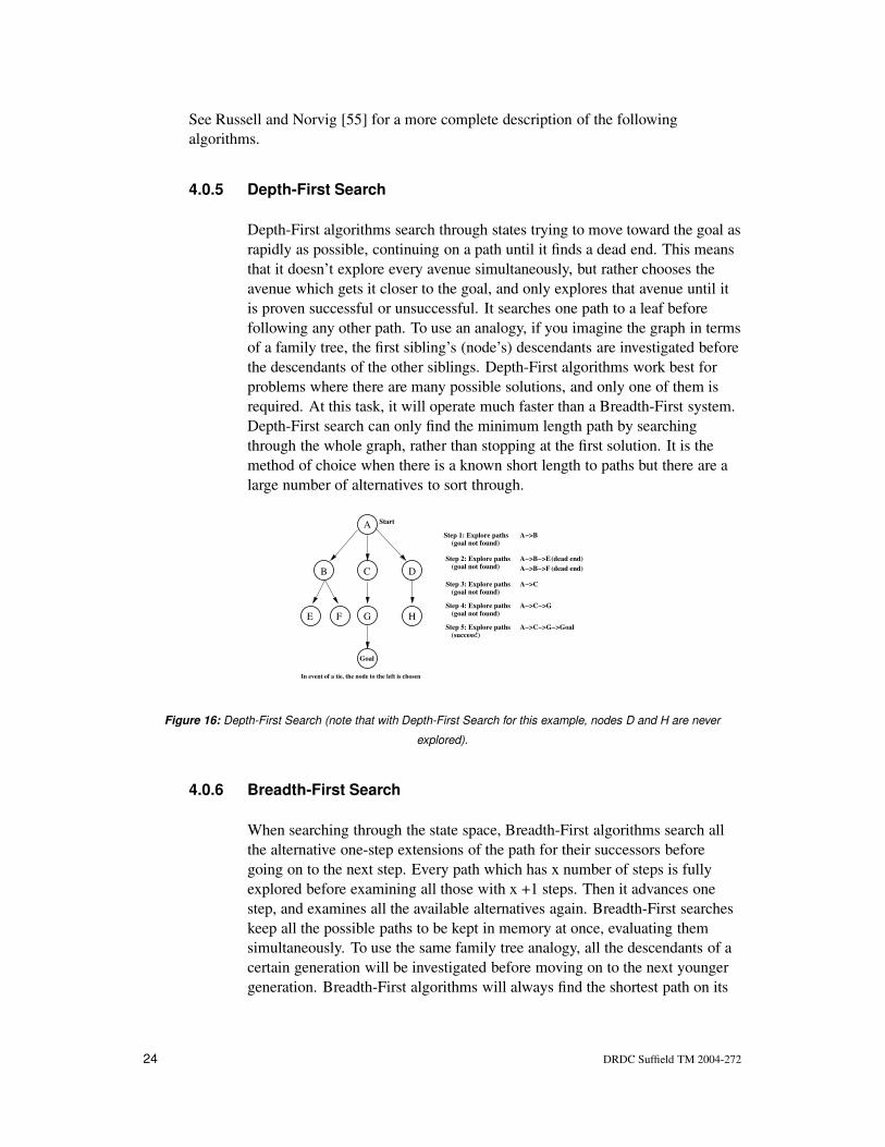
Figure 16. Depth-First Search (note that with Depth-First Search for this example, nodesD and H are never explored). . . . . . . . . . . . . . . . . . . . . . . . . . . . . . . 24

Figure 17. Breadth First Search. . . . . . . . . . . . . . . . . . . . . . . . . . . . . . . 25

Figure 18. Iterative Deepening Search. . . . . . . . . . . . . . . . . . . . . . . . . . . . 25

DRDC Suffield TM 2004-272 ix

Figure 19. Uniform Cost Search. . . . . . . . . . . . . . . . . . . . . . . . . . . . . . . 26

Figure 20. A* Search Algorithm. . . . . . . . . . . . . . . . . . . . . . . . . . . . . . . 28

Figure 21. Agent-Centered Search. . . . . . . . . . . . . . . . . . . . . . . . . . . . . . 31

Figure 22. Results for Framed Quadtree Representation. . . . . . . . . . . . . . . . . . . 34

Figure 23. Family Tree of Path Planning Methods . . . . . . . . . . . . . . . . . . . . . 36

x DRDC Suffield TM 2004-272

1. Introduction

A human driver looking at a map of a city, countryside or wilderness can quickly andefficiently decide on the best path to get where he or she is going. Humans canautomatically separate portions of the map symbolically in our minds, recognizehazards to our vehicle, roads which will take us there quickly, and effortlessly pick theshortest way to reach our goal. For robots this is not such an easy task owing to theirlack of ability to reason symbolically. A robot must first divide up the world into piecesit can recognize as obstacles, undesirable terrain, or dead ends. Then it mustsystematically search through the world to find the best route.

Through the Autonomous Land Systems initiative, Defence R&D Canada isinvestigating the area of Unmanned Ground Vehicles (UGVs). The goal is to createautonomous robotic vehicles which can be useful in a wide variety of applications,which can think for themselves and are not a burden to their users. One majorchallenge is giving vehicles the ability to find their way intelligently through a widevariety of terrains. This may mean finding suitable paths when given a complete map ofthe area in which the robot is to operate, or perhaps when given nothing more than asuite of sensors to view their world. In some instances it is possible to reach objectivesby blindly fumbling toward the goal. However, at other times, systems which arepurely reactive will take a long time in reaching their destination if they get there at all.A global world view with the ability to plan well into the future based on accumulatedinformation is a distinct trait of intelligent creatures which allows them to reach goalsquicker and avoid potentially dangerous situations. Principles of global path planningtherefore need to be applied for successful UGV applications.

This document is a survey of methods that have been developed by the roboticscommunity for path planning by robotic vehicles. The general intention of the survey isto provide guidelines for those methods which are most applicable to outdoor crosscountry navigation. However, because a great deal of mobile robot research hashistorically been focused on planning the paths of indoor robots and the movement ofrobotic manipulators it is important to consider the applicable lessons from thatresearch as well. In addition, a combination of the methods developed for indoor andcross country navigation will probably prove to be effective when implemented for pathplanning in urban environments.

Autonomous navigation by a UGV or mobile robot from one location to another is avery complex process. The robot must accomplish at least four simultaneous tasks to besuccessful and efficient:

1. Perception - Viewing the world and interpreting what it sees.

2. Localization - Keeping track of the robot’s position.

3. Local Navigation - Making sure the robot doesn’t tip, drive into holes or bump intoobstacles.

DRDC Suffield TM 2004-272 1

4. Global Path Planning - Finding the fastest and safest way to get from start to goal.

The subject of this survey is the fourth task given above: global path planning which isthe process of deliberatively deciding on the best way to move the robot from a startlocation to a goal location. In more technical terms it is defined by Dudek [12] as“determining a path in configuration space between the initial configuration of therobot and a final configuration such that the robot does not collide with obstacles andthe planned motion is consistent with the kinematic constraints of the vehicle”. Thefield of path planning borrows heavily from experience in other fields, such ascomputer networking, artificial intelligence, computer graphing, and decision makingpsychology. Although it is not the only type of cognition required, path planning isdefinitely a key component of autonomous intelligence.

There are a number of terms associated with path planning which are used in differentways by different people. Some are clarified here for the purposes of this report:

Navigation - A very diverse term which can have a variety of meanings. Generally itmeans “getting from here to there”, but it also encompasses the fields of pathplanning, motion planning, obstacle avoidance, and localization.

Global Path Planning - Planning which encompasses all of the robot’s acquiredknowledge to reach a goal, not just the current sensed world. It is slower, moredeliberative, and attempts to plan into the future. There is generally norequirement for it to run in real time, but instead is usually run as a planning phasebefore the robot begins its journey.

Motion Planning - This term can mean both the high level and low level planning forthe way that a robot will move, but must involve a deliberative aspect. This termis used more often in manipulator robotics or for planning on a smaller, morelocal scale. An example for a mobile robot is the classic parallel parking problem.

Local Navigation - The process of using only the robot’s current sensed informationof its immediate world to avoid obstacles and to ensure vehicle stability andsafety. It is much more reactive than path planning and runs in real time. Thespeed at which a vehicle can travel is limited by the speed at which the localnavigator can operate.

Obstacle Avoidance - Used in a very similar manner to local navigation, but wherelocal navigation considers vehicle stability, safety, and goal directedness, obstacleavoidance is concerned with merely getting around objects that are in the robot’sway.

Trajectory Planning - Planning the robot’s next movement. This term is synonymouswith motion planning.

Non-holonomic Path Planning - Requires the consideration of constraints which arenon-integrable and impose restrictions on possible state transitions. An example isthe inability of a car-like robot to move straight sideways.

2 DRDC Suffield TM 2004-272

Kinodynamic Path Planning - Accounts for constraints on the velocity andacceleration that a robot can accomplish.

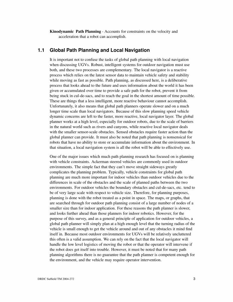
1.1 Global Path Planning and Local NavigationIt is important not to confuse the tasks of global path planning with local navigationwhen discussing UGVs. Robust, intelligent systems for outdoor navigation must useboth, and these two processes are complementary. The local navigator is a reactiveprocess which relies on the latest sensor data to maintain vehicle safety and stabilitywhile moving as fast as possible. Path planning, as discussed here, is a deliberativeprocess that looks ahead to the future and uses information about the world it has beengiven or accumulated over time to provide a safe path for the robot, prevent it frombeing stuck in cul-de-sacs, and to reach the goal in the shortest amount of time possible.These are things that a less intelligent, more reactive behaviour cannot accomplish.Unfortunately, it also means that global path planners operate slower and on a muchlonger time scale than local navigators. Because of this slow planning speed vehicledynamic concerns are left to the faster, more reactive, local navigator layer. The globalplanner works at a high level, especially for outdoor robots, due to the scale of barriersin the natural world such as rivers and canyons, while reactive local navigator dealswith the smaller sensor-scale obstacles. Sensed obstacles require faster action than theglobal planner can provide. It must also be noted that path planning is nonsensical forrobots that have no ability to store or accumulate information about the environment. Inthat situation, a local navigation system is all the robot will be able to effectively use.

One of the major issues which much path planning research has focused on is planningwith vehicle constraints. Ackerman steered vehicles are commonly used in outdoorenvironments. The simple fact that they can’t move straight sideways greatlycomplicates the planning problem. Typically, vehicle constraints for global pathplanning are much more important for indoor vehicles than outdoor vehicles due to thedifferences in scale of the obstacles and the scale of planned paths between the twoenvironments. For outdoor vehicles the boundary obstacles and cul-de-sacs, etc. tend tobe of very large scale with respect to vehicle size. Therefore, for planning purposes,planning is done with the robot treated as a point in space. The maps, or graphs, thatare searched through for outdoor path planning consist of a large number of nodes of asmaller size than for indoor application. For these reasons the path planner is slower,and looks further ahead than those planners for indoor robotics. However, for thepurpose of this survey, and as a general principle of application for outdoor vehicles, aglobal path planner will simply plan at a high enough level that the turning radius of thevehicle is small enough to get the vehicle around and out of any obstacles it mind finditself in. Because most outdoor environments for UGVs will be relatively unclutteredthis often is a valid assumption. We can rely on the fact that the local navigator willhandle the low level logistics of moving the robot or that the operator will intervene ifthe robot does get itself into trouble. However, it must be noted that for many pathplanning algorithms there is no guarantee that the path planner is competent enough forthe environment, and the vehicle may require operator intervention.


Uses immediate sensor data only Uses accumulated and a priori information

Plans for long distances and time periods

Slow, deliberative process

Allows robot to avoid getting trapped

Plan to reach goal in most efficient manner

Simple model of vehicle (point robot)

Concerned with hills, rivers, canyons, forests,roads, buildings, etc. bumps, logs, etc.

Concerned with rocks, holes, slopes,

Fast and reactive

Allows robot to travel safely

Plan to travel as fast as possible

Complex vehicle model (dynamics and kinematics)

Local NavigationGlobal Path Planning

Plans for immediate vicinity for a short time ahead

Figure 1: Global Path Planning vs. Local Navigation

1.2 Path Planning Concerns

Given an initial position and orientation, as well as a goal position and orientation, apath planner’s job is to calculate a path which specifies a continuous sequence ofpositions and orientations in order to avoid contact with obstacles. It should reportfailure if no such path exists. Historically, the path planning problem has been studiedmuch less for outdoor vehicles than for indoor vehicles. This may be because outdoorenvironments are much less cluttered than indoor, but is more likely that the ease of use,size and complexity of indoor mobile robots make them ideal experimental vehicles.This document attempts to analyze the methods presented in terms of effectiveness foroutdoor path planning, from which indoor path planning has a great many differences.Indoors, the terrain is flat and vehicle stability can safely be ignored. Obstacles are welldefined and regular, and a binary obstacle/no obstacle representation is almost alwayssufficient. Outdoor environments have some of the following complications:

• The range of obstacles is large, a robot must dodge rocks as well as mountains.

• Vast areas of terrain are often not mapped at high enough resolution for planning.

• Negative obstacles such as ravines, holes, and ditches pose a threat.

• Tipping hazards for robots exist.

• Outdoor areas often contain large areas of sparsely populated terrain, punctuated bycluttered areas.

• Widely varying traversability exists, such as mud, pavement, tall grass, bushes,trees, and rock piles.

Any navigation system for a UGV will need to incorporate all of these concerns inorder to be effective. Nevertheless, many methods developed for indoor robots haveapplicability for outdoor vehicles but would require adaptation for efficient use. Forexample, a river with a bridge across it will be much larger than a wall with a door in anoffice, but they represent similar challenges to the robot but on a different scale. In anyevent, there are many similar characteristics which all path planners have:


Search Space: This represents the possible states, or positions, orientations andconditions of the robot, the world and its objects. A simple example is the x,ycoordinates of a vehicle in the Euclidean space. More complex states may involveconditions as complicated as radio signal strength or fuel level.

Actions: A plan must also generate actions, or ways of moving from state to state.

Time: Planning always involves time in some way, even if not explicitly. A plannermay include time in such ways as: “at time t the robot will be at point x,y”, or“the path should take the least amount of time possible.” Usually time isrepresented simply as a sequence of actions: “after Action A is completed therobot will do Action B”.

Initial and Goal States: The plan is the way the robot will get from the initial to thegoal state.

Criteria For Planning: The desired characteristics of the “best” plan, such as time,distance, or safety. These are yardsticks by which to optimize plans.

Constraints: Those items which limit the range of plans that can be made, such asmaintaining vehicle safety, stealth or the physical limitations of the robot.

Algorithm: This is the method by which the best plan is obtained given the criteriaand constraints for planning.

Plan: The sequence of actions to move from the start configuration to the goalconfiguration.

There are a number of considerations for path planning that will influence the design ofthe system and criteria by which they are judged:

Environment: Does path planner sufficiently represent the environment? Is theapplication indoor or outdoor? Is it cluttered or relatively open?

Robot Structure: Does the path planner provide a sufficient but not excessivelydetailed representation of the vehicle with respect to size and mobility constraints?

Optimality: Requirements can be based on minimum distance traveled, time taken,vehicle safety, etc.

Completeness: Will it find a path if one exists?

Space and Time Complexity: Can it operate fast enough so the robot does not need tostop and think?

Dynamic or Unknown Worlds: Can the path planner deal with changing informationor goals?

For some other general information regarding mobile robot path planning see[12][44][33][35] [34].


1.3 Overview of Report

The methods for planning are very closely tied with the world representations used. Inorder to plan a path for a robot, the world must be represented, in order to define thatportion of the world in which can be travelled through (free space), that portion thatcan’t (obstacles), and sometimes that part which can be travelled in, but is undesirable(traversability analysis). Therefore, the first section of this report is all about thevarious ways that the information about the world can be represented within the robot.It covers topological and metric path planning, the idea of a configuration space, anddiscrete vs. continuous state spaces. The second section surveys specificrepresentations which have been applied to the path planning problem, such as celldecompositions, road maps and potential fields. Once the world is represented withinthe robot the path planner will need to search through the representation for the bestpath to the goal using algorithms such as Depth-First, Breadth-First, and Heuristicsearches presented in the third section. The final piece of the path planning problem isusing information accumulated from sensors. The final two sections survey thesemethods, which are the most recently developed and most effective for global pathplanning in outdoor environments.

This report is a survey of global path planning, not local navigation techniques. It doesnot cover sensor based motion planning techniques, planning algorithms which planvehicle action on a local scale, or systems which enable rough terrain mobility. This isnot to say that the techniques here do not allow for replanning and the consideration ofsensor acquired data but that the main planning function goes on within the space ofpreviously acquired information. This survey also gives little consideration to planningwith non-holonomic constraints and kinodynamic planning. This is not to say that theplanning algorithms presented below cannot be used on vehicles with these types ofconstraints, but rather the planning is done at a high enough level and over a longenough time scale that they are unimportant factors.

2. World Representation for Planning2.1 Topological vs. Metric Path Planning

Humans use two types of navigation and representation: topological navigation andmetric navigation. Topological navigation operates on landmarks and identifiablelocations such as intersections. Directions are given in terms such as “go to the big tree,turn left and cross the river”. Topological methods can go by many other names such asqualitative, route based, or landmark navigation. They express space in terms ofconnections between identifiable locations such as landmarks and intersections, and aredependent upon perspective of the robot (i.e orientation clues are egocentric).Topological representations cannot be used to generate metric representations eventhough the reverse is true. The representations are used in a more reactive way and aremore robust to localization errors. Unfortunately most of the research in this field hasbeen undertaken for indoor environments where the identifiable nature of objects


enable a vehicle to easily find landmarks. It is more difficult in outdoor environmentswhere a sparsity and lack of uniqueness makes topological cues harder to find.Topological methods may use waypoint navigation, visibility graphs, or voronoidiagrams which are all described below. For some typical examples of topological pathplanning implemented on indoor robots, see works by Park[48] or Thrun[64].

On the other hand, metric navigation lends itself well to outdoor environments eventhough it requires more competent localization. Metric methods favor techniques whichproduce an optimal path and express directions in terms of physical travel, often from abird’s eye view. The map structures are independent of orientation and position of therobot. In metric navigation, directions are given in specific geographic terms withdistance and direction, such as “travel at 30 degrees for 300 metres then at 170 degreesfor 100 meters”. Metric paths are usually described as a set of waypoints or subgoals,defined in the (x, y) coordinate system. Often GPS can provide a global coordinateframework. In addition, metric navigation lends itself very well to computer datarepresentation, and computational search algorithms. The metric methods shown laterin this report are potential fields and cell decompositions.

Figure 2: Topological and metric representations.

2.2 Planning Space2.2.1 Configuration Space

In path planning for mobile robotics, the vehicle and the world through whichit travels must both be represented in some manner so that plans can beevaluated in a search space. The search space represents all the possiblesituations that can exist. In order to plan a robot’s motions when there aremany degrees of freedom, a construction called a configuration space is used.At every point in time, a robot can have exactly one combination of itsposition and orientation. This unique combination is called a configuration. Aconfiguration space (c-space) represents each possible configuration as asingle point and contains all of the possible configurations of the robot. All ofthe physical obstacles from the robot’s working space are mapped ortransformed into this configuration space. This c-space is used where thecombination of position and orientation is mapped into a single configurationpoint, because it transforms the problem from planning complex objectmotion to planning the motion of a point.


For example, consider a single rigid, wheeled mobile robot, operating in a twodimensional environment. A configuration space which has three dimensionscould be used: position x, position y, and orientation angle. Each node in theconfiguration space will be a unique combination of these three dimensions. Ifthe planning is at a high enough level or if the vehicle is capable of holonomicmotion, the configuration space can be reduced to the two dimensional x and yspace. For example, if orientation is not a concern, all the positions of amobile robot could be represented in an (x,y) grid, and the sequence of (x,y)positions the robot will occupy in order to reach the goal then planned.However, what if the world is cluttered, and the vehicle is a car-like robotwhich has strict conditions of movement for safety, and a limited number ofmotions it can control? In this case, the vehicle orientation becomesimportant. Now a larger number of dimensions in the working space (x,y andtheta) must be considered, and a configuration space can aid the planning. Ifplanning is done in a three dimensional world then one may have to use up to6 dimensions in the configuration space (x,y,z positions, as well as roll, pitchand yaw).

A good choice of configuration space will contain the fewest number ofdimensions to allow the planning algorithms to work quickly. As degrees offreedom are added for a complex system, the configuration space growsquickly in size and number of dimensions, making planning much moredifficult. Unfortunately, as it has been suggested by Latombe [33], theplanning problem grows exponentially in time with the number of dimensionsin the configuration space. This means that the fewer the number ofdimensions that need to be considered the better. For this reason, researchersoften use simplifications of the problems to attain faster performance of a pathplanner. For global path planning, the possible configurations are oftenreduced to simply the x,y co-ordinate space.

2.2.2 Discrete vs. Continuous Space

In representing the world for robot path planning a continuous or discretesearch space can be used. A continuous state space models the world as acontinuous set of an infinite number of possible states. Path planning thenmeans finding a continuous trajectory which navigates this space. In general itis more difficult to do planning in a continuous state space, as the mathematicsinvolved become complicated. The continuous state space is more often usedfor reactive obstacle avoidance rather than for global path planning where thecomplexities overwhelm its usefulness.

When using a discrete state space the search space is broken up into a finitenumber of possible discrete states that the vehicle can reside in, and describesany number of characteristics of that state, such as position and pose forvehicles, or elevation, slope, roughness, etc. for an environment’s state space.


In order to produce a plan each of these discrete states has a state transitionfunction to determine the other states directly reachable from it. An algorithmexplores the state space to find a sequence of states which define a path fromthe original state to the goal state. This search algorithm may operate on anynumber of different rules which guide it to find the optimal path based onwhatever criteria the designer intends. Another way of thinking of the discretestate space is as a set of nodes with links between them. Links can have costs,and a path is a sequence of nodes connected by links.

This discrete vs. continuous state space consideration can be applied on manylevels. For example, if a planner was searching for a steering angle for avehicle, it could search through a number of discrete candidate steeringangles, or it could do a mathematical maximization on the continuous set ofall possible steering angles. As another example, potential field methods ofpath planning can be applied to a continuous field defined by mathematicalfunctions, or the functions can be discretized into a grid map which the pathplanner searches through.

3. Representation and Path Planning

Most methods of planning use one of three types of configuration space representation,called roadmap, cell decomposition and potential fields. Roadmaps model connectionsbetween special points, cell decomposition methods break the world into grids, andpotential fields apply mathematical fields to model the world. Of these three methodscell decomposition is the one most widely used for outdoor robotics. Each of thesetypes may be either topological or metric in nature. All the methods mentioned belowin general must be discrete, except for the Potential Field method, which can also beimplemented in a continuous state space fashion.

3.1 Cell Decomposition Methods

Cell decomposition methods are the most studied and widely applied methods foroutdoor robotics. In these methods the planning space is broken up into discrete,non-overlapping regions which are subsets of the c-space and whose union is makes upexactly the entire c-space. The result is a graph in which each cell is adjacent to othercells. The methods for traversing from one cell to adjacent cells is called theconnectivity graph. A planner then searches through the connectivity graph and thepath generated is a sequence of cells the robot should traverse to reach the goal. Thecost of traversing a cell may vary and the planner must apply a metric to determinewhich is the optimal path. Cell decompositions are often used to represent the physicalspace itself, but can also be used on a configuration space.


3.1.1 Approximate Decomposition

Approximate cell decomposition is created by laying a regular grid over theplanning space. The cells of the grid are of a predefined shape and size, andare therefore easy to apply. If there is an object in the area contained by thegrid element, that element is marked as an obstacle. Otherwise it is left as freespace. The center of each cell becomes a node in the search graph that will beexamined to find a path. As shown in Figure 3, these nodes can either be4-connected or 8-connected representing whether or not the robot isconsidered to travel diagonally between them. Rather than identifyingparticular objects or shapes, the cell decomposition simply samples the worldand marks up the graph accordingly as to whether the space is full, empty orpartially full. Two dimensional binary representations are called bitmaps, andif they have a range of values, occupancy grids. Three dimensional gridelements are known as voxels. This method is called “approximate” becausethe boundaries of physical objects in the world do not necessarily coincidewith the predefined cell boundaries. Approximate cell decomposition ispopular for a number of reasons: the algorithms are easier to implement thanthose for other representations, they are simple to apply to a world space, andthey are flexible. The cells size can be tuned for reducing computation time byincreasing the cell size, thus reducing the number of cells to search through, orby reducing the cell size to provide more completeness and detail. This makesthem appealing for mobile robots where paths must be re-calculated on the fly.

��

��

��

��

��

��

��

��

� � �

��

��

��

��

��

��

��

��

��

Figure 3: 8-connected and 4-connected grids.

However, there are a few problems with this method despite its ease of use.The first is digitization bias. In cell decomposition methods an obstacle muchsmaller than the grid size will result in that entire grid square being labelled asoccupied. This results in a conservative estimate of the free space, and spacethat is passable might be considered impassable by the planner. In effect if thegrid resolution is too coarse there is no guarantee of finding a path where oneexists (i.e. it is non-complete). This problem with approximate celldecomposition is illustrated in Figure 4 to a somewhat exaggerated extent. Tocombat this a finer scale grid is used, which then means higher storage andcalculation costs for path planning. Also, the complexity of these methodsgrows quickly with the dimension of the c-space so they are realisticallyapplicable only when the c-space has dimensions of around 4 or less.Approximate cell methods were introduced by Brooks and Lozano-Perez [6],and expanded by Zhu and Latombe [70] as well as many, many others since(see the Section 4.0.9 on Trulla and Section 5.4 on D* below for examples).


Figure 4: Incompleteness of approximate cell decomposition. The bridge is labelled as blocked because the gridhas resolution which is too low. Also note the inefficiency of the regular grid in the open spaces.

When using approximate cell decomposition the system can use one of manytypes of shapes to divide up the c-space. Regular cell decomposition usingsquare cells seems to be the dominant method of representation for outdoorvehicles. Regular grids have an innate ability to be general, as there are noassumptions about the size and shape of objects inherent in the representation,which is good for outdoor environments.

The cells in the decomposition will have costs associated with traversingthem. If this cost is a binary value the map simply contains obstacle and freespace regions, which is very common for indoor robotics. However, one canalso assign a wider variety of values to the cell cost, resulting in a graph thatdescribes traversability of an area with more flexibility, as outdoor obstaclesrarely have easily definable boundaries. For example, to the map cells in amap for an outdoor world one could assign many different costs of traversal,such as roughness, slope, trafficability, etc, which can then be combined toform a total cost value. This flexibility in representation allows for a powerfulpath planning mechanism.

3.1.2 Adaptive Cell Decomposition

Adaptive cell decomposition is used to reduce the number of cells used inopen areas (in order to waste less memory storage space and computationtime), and to remove the digitization bias of the regular cell decomposition. Itis a good tactic for expansive natural terrains in which there are large areaswith the same traversability. Adaptive decomposition relies on the fact that


much of the information in the free space is redundant in a regular celldecomposition. The regular shape of the cells is maintained, but the cells arerecursively reduced in size in order to both use the space more efficiently andmaintain as much detail as possible. The result is less memory required andless processing time.

The most common type of adaptive decomposition is a quadtree as shown inwork by Samet [57] or Naniwa[45]. It begins by imposing a large size cellover the entire planning space. If a grid cell is partially occupied, it issub-divided into four equal subparts, which are then reapplied to the planningspace. These subparts are then subdivided again and again until each of thecells is either entirely full or entirely empty. The resulting map has grid cellsof varying size and concentration, but the cell boundaries coincide veryclosely with the obstacle boundaries. A simple quadtree representation isshown in Figure 5.

Unfortunately, adaptive cell decomposition imposes problems for dynamicenvironments where the robot is acquiring new data and updating its mapbased on new obstacles. When this happens, it is necessary for the entire datastructure of the map to be completely revamped. There is also some difficultyusing quad-trees with continuous cost maps, which are more useful on naturalterrain, because you cannot subdivide the world into free and occupiedregions. In addition, quad-trees have difficulty in providing near optimal pathsand often result in jagged paths. One good solution is framed quad-trees assuggested by Chen [7]. As can be seen by comparing the regular quad-tree inFigure 5 with the framed quadtree in Figure 6, a much better path can befound. However, in high clutter environments framed quad-trees can be lessefficient than regular grids, due to the overhead required to keep track of thecell sizes and locations.

3.1.3 Exact Cell Decomposition

Exact cell decomposition attempts to solve some of the problems with regulargrids in a different way. The cells do not have a predefined size or shape, butare determined based on the world map and the location and shape ofobstacles within it. The cell boundaries correspond exactly with theboundaries in the planning space, and the union of the cells is exactly that ofthe free space in the world. This makes exact cell decompositions complete inthat they will always find a path if one exists, but they will not result inoptimal (shortest) paths. Unfortunately, there is no simple rule for how todecompose the space into cells. This method is quite difficult to apply foroutdoor environments where obstacles are often poorly defined and ofirregular shape. It also does not lend itself well to the use of scales oftraversability (as opposed to using binary obstacle and free-space regions).See Schwartz[58], or Avnaim [1] for examples of exact representations. A


start

goal

Figure 5: Quadtree representation.

start

goal

Figure 6: A framed quadtree.


summary of the application of exact cell decomposition for path-planning isgiven by Sleumer [59]. One type of exact cell decomposition is shown inFigure 7.

Figure 7: One type of exact cell decomposition.

3.2 Roadmap Methods

The second major type of representation for path planning are the Roadmap Methods.Roadmaps are graphs which represent how to get from one place to another. Roadmapmethods of planning find the connections between the robot’s free space as a set of onedimensional curves. Once the roadmap has been constructed it is used as a set ofstandardized paths which the planner will search through to find the optimal solution.The nodes in the graph are usually waypoints that the robot needs to travel between fora successful journey. A topology based road map graph will put the nodes of the graphat distinctive locations which the robot can identify. Roadmaps provide a hugeadvantage over cell decompositions in the number of nodes a planner needs to searchthrough in order to find a path. The set of nodes doesn’t consist of all of theconfigurations, but a select few that are special. This makes them harder to create, buteasier to manipulate and use. On the downside, roadmaps are generally difficult toupdate or repair as the robot gains new information, because the entire roadmaptypically needs to be remade. In addition, most of the methods of creating the graph useartifacts of the map, such as corners of objects or crossroad to generate the landmarksand area boundaries, rather than things that can be sensed by the robot.

3.2.1 Visibility Graphs

One of the earliest roadmap methods, which applies to 2 dimensionalc-spaces, is the visibility graph, which was used on Shakey[47]. The visibilityroadmap consists of straight line segments which connect the nodes of thepolygonal obstacles, without crossing the interior of the obstacles, as inFigure 8. These straight lines make up the paths on which the robot maytraverse, and the optimal path is selected by any of a number of searchtechniques, explained in more detail later in this report. Visibility graph


methods are poor because the calculated paths are tangential to the obstaclesand the robot will brush right up against the obstacles. In order to account forthis obstacle regions are generally grown to provide a safety margin, althoughthis results in incompleteness and inefficiency of the planner. Anotherproblem is that the obstacles must be clearly defined polygons. This is aproblem for outdoor robots because obstacles almost always take on round oramorphous shapes. A simple visibility graph is shown in Figure 8. In thisexample the possible paths which can be taken by the roadmap are shown insolid lines connecting the corners of the obstacles, and the shortest paththrough the roadmap, which the robot would take, is shown as the dotted line.

start

goal

Figure 8: A visibility graph.

3.2.2 Voronoi Diagrams

A voronoi diagram[10] is another popular mechanism for generating aroadmap from a c-space. It can be constructed as the robot enters a newenvironment. The roadmap consists of paths, or voronoi edges, which areequidistant from all the points in the obstacle region. A rough Voronoidiagram is shown in Figure 9. The points where these edges meet are calledvertices, and often have a physical correspondence to aspects of theenvironment which can be sensed, such as intersections of hallways. Incontrast to visibility graphs, Voronoi paths are by definition as far as possiblefrom the obstacles. If a robot follows a voronoi edge, it won’t collide with anymodeled obstacles, and there is no need to grow obstacle boundaries. Thismakes Voronoi methods safe, but the paths generated inefficient.

3.2.3 Probabilistic Roadmaps

A much more recent advance in the roadmap methods is the ProbabilisticRoadmap (PRM) [22], which attempts to make planning in large orhigh-dimensional spaces tractable. A PRM is a discrete version of acontinuous c-space which contains much fewer states than the originalc-space. It is generated by randomly sampling the larger c-space and then


start

goal

Figure 9: A Voronoi diagram.

connecting those points into a roadmap. PRMs are an improvement becausemost other planners, especially cell decomposition ones, try to solve theplanning problem in the entire search space. PRM methods solve in aroadmap built from a randomly chosen subset of the search space and then usea computationally inexpensive search algorithm to finish the job. PRMs arebased on the premise that a relatively small number of points and milestonesand paths are usually sufficient to capture the connectivity of free space. Thisassumption can greatly accelerate the planning process.

Path planning using a PRM has two phases, consisting of a construction of theroadmap phase and path query phase. To construct the map random points inthe configuration space are chosen and added to a list of special points. If apoint lies in the obstacle region it is discarded. The mapping algorithmattempts to connect this point to a subset of the other configurations already inthe list of special randomly chosen points. This connectivity is usuallyevaluated very simply by using a straight line between the two points, and notconnecting them if an obstacle is in the way. This process of random selectionand then evaluating connectivity is repeated a large number of times. Thiscreates a list of the available connections between the points that wererandomly chosen. This list of connections is the roadmap, which defines aseries of waypoints around obstacles in the c-space. In the query phase, whenthe robot needs to plan a path between two configurations, the algorithm usesthe roadmap created in the first phase to search through the waypoint nodes tofind the least-cost path between the start and goal configurations. The initialgraph building process is computationally expensive, however, once it hasbeen constructed, the search is very efficient. A simple example of a RPM anda path from start to goal is shown in Figure 10.

One problem with a standard PRM method is that it is inefficient for narrowconfined spaces. Because the points which make up the roadmap are chosen atrandom, the chance of catching a random point in the tight space is low, andno connectivity will be established between sections of the map, as shown in


Randomly chosen points

Paths searched by algorithm

Start

Goal

Figure 10: PRM with randomly chosen nodes.

Figure 11. Greater coverage with a greater number of nodes leads to betterpaths and more chance of getting through tight spots, but makes the planningmore complex. This problem has been tackled by Boor[3] and others.

Figure 11: A poorly covered and a well covered PRM.

Another problem with PRMs is that they are usually based on binary obstaclesthat most other roadmap planners use, rather than a gradual costing. Thismeans that obstacles need to be well defined and generating variable pathcosts is more difficult than with other methods. A third problem with PRMmethods occurs when obstacles are added or removed from the map and theentire roadmap must be regenerated. Because generation of the roadmap isslow and cannot be done in real time, the planner functions poorly when theinformation is changing often or if the initial information is incorrect. Thatsaid, however, the roadmap construction is incremental, and can be expandedas necessary when the robot explores new terrain. Work has been done toalleviate the problems with PRMs by Hsu [19], Leven[38] and others toovercome the dynamic obstacle limitation. There are also many othervariations of PRM planners presented in the literature.


3.2.4 Rapidly Exploring Random Trees

A further variation of PRMs is the Rapidly Exploring Random Tree (RRT).Rather than randomly sampling the configuration space as a PRM does theplanner begins at the start location and randomly expands a path, or tree, tocover the configuration space. The main focus is to build a roadmap in afashion which draws the expansion of the connected paths toward the areaswhich have not been filled up yet. The planner pushes the search tree awayfrom previously constructed vertices. This allows them to rapidly searchlarge, high dimensional spaces. They are also well suited to the capture ofdynamic or non-holonomic constraints, which with PRM methods havedifficulty (although this capability is not critical for high level global pathplanning). One method for planning, as shown in Figure 12, is to grow twoRRTs, one from the goal and one from the start, and then search for states thatare common to both, creating a linked path between the two. For examples,see “Randomized Kinodynamic Planning” by Lavalle [36], and others byKuffner [32], Cheng[8], and Frazzoli[14].

Start Goal

Start Goal

Figure 12: Path planning using RRTs. The roadmap paths are grown in linear increments from both the goal andthe start positions. When the two paths grow within a certain distance of one another, they are connected, and the

robot can follow the path to reach the goal.

3.3 Potential Fields

Potential Fields is the third major type of representation used in path planning.Potential Field methods are quite different from the previously discussed methods ofplanning, and have been used extensively in the past. Instead of trying to map thesearch space they impose a mathematical function over the entire area of robot travel.This method treats the robot as a point under the influence of fields generated by thegoals and obstacles in the world, much like an electron in an electric field. Obstaclesgenerate repulsive forces and goals generate attractive forces. These forces are stronger


near to the obstacle or goal and have less effect at a distance. At every space in theworld the resultant force of the fields on the robot determines the direction of motionthe robot should take. Even though a mathematical function is used, the search spacecan still be either discrete or continuous. Potential Fields were originally devised forreal-time obstacle avoidance with emphasis on real-time efficiency, not path planning.The method was based on information gained from sensors, rather than a prioriinformation (see Khatib[23]). These methods were expanded by Latombe [33] as wellas countless others. The methods are relatively easy to implement, and arecomputationally efficient. Unfortunately Potential Fields have the flaw of containinglocal minima other than the goal in which the robot can get stuck, as is shown in Figure13. Much of the efforts of adapting potential fields have been at overcoming this flaw.

Goal

Start

23333

333 3 3 3

33

222222222 2 2 2 2 2

2222

1211111111

111111 1

1111

Potential field for Obs2b)

Goal

Start

11 1

2

22

2 23333

333

444444444

55555555555

666666666

66

777777777

77

8888888888

88

89999999999

999999999

1010101010101010101010101010101010101010

88

Potential field for the goalc)Goal

Start

11 1

2

22

2 2333

78

88

99999

101010101010

4444

5556766667

88899 9 8 7 7 7

8991010989

10

989

10

1098

8 9 10 10 9101111109

9101111111110

11121212121110

11111111111110

12121212121211

11111111111111

Local minima here

Sum of potential fields from Obs1, Obs2 and Goald)

Goal

Start

33 3 3 3

333333 2

22222222

Value of potential field

Obstacles

3

222222 2 2 2 2 2

1111111 1 1 1 1 1 1

due to first obstacle

Potential field for Obs1

at this point

a)

Figure 13: Simplified potential fields. Field produced by obstacles in a) and b), the field produced to create goalattraction in c), and the sum of the fields in d). This summed field will be used to direct the robot along the levels of

lowest potential. Note the local minima that will cause the robot to be trapped.

Potential fields are often referred to as a local method, as opposed to a global method,because the effect of the field on the robot is almost exclusively based on obstacles near


it. Obstacles far away have little to no effect on the robot’s motion, and so it can’t be auseful planning method. One simple method of making potential fields a planningmethod is to forward simulate the motion of the particle in the field, and then use thatsimulated motion as a planned path. However, there are simpler and more efficientways to use the potential field for path planning which are described below.

3.3.1 Navigation Functions

The local minima problem can be overcome in one of two ways: 1) byincluding techniques for escaping minima or 2) with the definition of potentialfield which has no or few minima. If a potential field that had only oneminima was created, then a path from the start to the finish could easily beplanned (this is called a global navigation function). There are a very largenumber of ways to define the potential field, but as was shown byKoditschek[24], it is not possible to create one with no local minima (you willhave one saddle point in the field for every obstacle). It is more practical tosolve the minima problem by constructing a navigation function, which has acertain small number of equilibrium points (an “almost global navigationfunction”). These equilibrium points will be unstable so that any smallamount of noise will allow the planner to avoid them. This is equivalent totaking solution 1 above (escape the minima). As for solution 2 (making apotential function with few minima), there have been many methodsdeveloped. See Koditschek and Rimon [25][54] for examples. However, it iscomputationally complex to define these navigation functions, and therefore isnot that practically useful. Rather than defining these potential functions overfree space, it is much easier when the c-space is represented in the form of agrid, such as is done for cell decomposition methods. The potential functionover the grid is called a numerical navigation function.

Once more, due to the requirement to discretely model obstacles, potentialfields are less useful for outdoor robotics. They are generally more efficientthan the graph search methods and don’t require an initial processing step toconstruct the connectivity graph of the configuration space. This makes themuseful as a local obstacle avoidance mechanism, due to the ease of calculationonce the potential function has been defined. The robot can simply move fromone configuration to another by evaluating the resultant vector. As you getmore degrees of freedom in the robot and more dimensions in the c-space, itbecomes much more difficult for a designer to come up with an appropriatepotential function. As a result potential field methods are limited as aplanning method and have fallen from favour.

3.3.2 Depth-First Planning and Potential Fields

Using Depth-First planning, a path is iteratively generated as a series ofstraight path segments through the configuration space[33]. Each segment is


generated from its start point in the direction of the resultant potential field atits start point. The length of the segment will be equal to some predeterminedlength. The calculation point, or start point, for the next segment is then theend point of the previous segment. The segment length is chosen to be smallenough to ensure no collision with obstacles, and that it will not overshoot thegoal. This method descends on the steepest part of the potential function untilthe goal configuration is reached. However, it has problems with local minimawhere it can easily become trapped.

3.3.3 Best-First Planning and Potential Fields

Best-First search in potential fields[33] retains a wider number of search pathssimultaneously, and is more robust to local minima. It involves constructing atree whose nodes are configurations in the c-space, and whose root is the startposition. At every iteration the algorithm evaluates the neighbors in thec-space of those leaves which have the lowest potential value in the field ofthe configurations investigated so far. The neighbors are then installed in thelist of nodes to evaluate with a pointer toward its parent, and the algorithmrepeats until the goal is reached. If the most active branch should terminate ina local minimum, another branch will be actively investigated until either it issuccessful, or the previous branch’s local minimum has been overcome (theminimum has been “filled up”). Once the goal has been reached the algorithmfollows the backpointers to the start position to define the planned path.

3.3.4 Wavefront Based Planners and Potential Fields

It is possible to create these grid based navigation functions with no minimaand plan the path to the goal in one step using a wavefront based planner. Thebasic idea is that the c-space is considered to be a conductive material, and thewavefront is heat radiating out backward from the goal to the start position.The planner calculates the potential at each node (cell) in the graph as thedistance from the goal as it propagates outward. The output of the wavefrontpropagation is a grid with each location containing the distance to the goal.Once the start position has been reached by this propagation, the planner canstep back through those cells with the lowest potential to achieve the path tothe goal.

A simplified generic wavefront plan and one possible path are shown in Figure14. The numbers in the cells represent the cost of any path at that cell, whichin this simplified case is the number of cell transitions (distance) to reach thegoal. In this example, the influence of the potential field from the obstacleshas been omitted for clarity. The effect of including the obstacles’ potentialfields would be to increase the costs of the cells which border the obstacles.

Two examples of potential fields and wavefront planning are the NF1 and NF2


navigation functions proposed by Latombe and Barraquand [33][2]. Thispotential field/wavefront method has also been implemented in thePlayer/Stage environment [15]. A simple illustration of wavefront planning isshown in Figure14. In this example, the number of transitions from the start tothe goal are shown in the grid. The robot could simply follow the decreasingvalues in order to reach the goal, and could do so along a number of differentpaths in this example.

goal

start

1

1 1

2

2

2

3

3

3

4

4

4

5

5

5

6

6

6

7

7

77

8

8

8 8

9

99

9

9

7

8

10

10

10 10

1010

10

11

11

11 11

11

11

12

12

1212

1212

12

13

13

1313

1313

13

13

13

14

14141414

1414

14

14

14

14

14

15151515

15

151515

16 16 16

16

1617

17

171717

18 18 18

18

1819

1919

Figure 14: Simplified wavefront planning.

NF1, which was implemented by Lengyel [37], is simple and finds the pathwith the shortest distance, but has a problem in that it produces paths whichgraze obstacles. This may be satisfactory if the scale of the plan is high levelenough, and you have a local reactive navigator. Brock [5] used NF1 in justthis fashion.

NF2 is a similar wavefront propagation technique to NF1, except that it findspaths that are as far away from obstacles as possible, in a similar manner toVoronoi roadmaps. NF2 is more complicated and no longer finds the shortestpath to the goal, but gives the robot a larger margin of safety and more roomto maneuver. Other wavefront propagation methods include Trulla[42] asdescribed in Section 4.0.9 and Mitchell[41].

4. Graph Search Algorithms

Once a method of representing the environment has been established, it is thennecessary to search for the best path through that representation. Graph searchalgorithms are used with the cell decomposition or roadmap methods of path planning,and also with the potential field methods, as shown in the previous section. Thesesearch algorithms come from a wide variety of applications including general problemsolving, artificial intelligence, computer networking, and mechanical manipulation.


They systematically search through a graph with the goal of finding a particular node.In the case of mobile robotics they search a roadmap or cell decomposition c-space.The side effect of this search for a particular node, the goal, is that if you keep track ofthe moves the search algorithm made to find the goal node, you have a path. The simpletrick for keeping track of this path is to label each node with its parent node with abackpointer. The string of backpointers defines the path.

Accumulated sensor data Representation− Cell Decomposition− Potential Field− Roadmap

Graph Search Algorithm − Breadth−first− Depth−first− A*− Wavefront− D*

Path

A priori information

Figure 15: The path planning process.

For UGVs, the search space is usually a two dimensional geographic world map whichhas been broken into a grid, where the individual states are grid cells, or physicallocations in the world map, and the states reachable from any given cell (state) arethose immediately surrounding it. The path defined by the algorithm will then be asequence of grid cells the robot should traverse to reach the goal. Algorithms for UGVsusually attempt to optimize this path based on fewest number of grid cell transitions (asan approximation for distance traveled). As an alternative, a cost can be assigned totraversing each node. In addition to the typical distance metric, many more variablesand costs to the planning space can be added. The global space can be marked up withtraversability, roughness hazard, slope hazard, boundaries of operation, communicationability, and so on. In this way, the representation is more flexible, intelligent and hasmore fidelity to the real world. When the paths are evaluated, the path length no longerdetermined by the number of nodes it has traversed, but by the sum of all the costs oftraversals on that path. For example, Saab and VanPutte’s system [56] can evenevaluate paths based on energy expended going up and down hills.

Many graph search algorithms require that every node in the graph be investigated todetermine the best path. This works well when there are a small number of nodes, suchas in a Voronoi diagram. However, when planning a path using a regular grid map overa large area this becomes very computationally expensive. Therefore, there are manyways to traverse the graph with many adaptations of two basic themes known asBreadth-First and Depth-First search.

Algorithms are evaluated based on three priorities:

Completeness - Is it guaranteed to find a solution if one exists?

Optimality - Is it guaranteed to find the least cost path?

Time/Space Complexity - What is the time and memory use of the algorithm, as thenumber of states in the graph increases?


See Russell and Norvig [55] for a more complete description of the followingalgorithms.

4.0.5 Depth-First Search

Depth-First algorithms search through states trying to move toward the goal asrapidly as possible, continuing on a path until it finds a dead end. This meansthat it doesn’t explore every avenue simultaneously, but rather chooses theavenue which gets it closer to the goal, and only explores that avenue until itis proven successful or unsuccessful. It searches one path to a leaf beforefollowing any other path. To use an analogy, if you imagine the graph in termsof a family tree, the first sibling’s (node’s) descendants are investigated beforethe descendants of the other siblings. Depth-First algorithms work best forproblems where there are many possible solutions, and only one of them isrequired. At this task, it will operate much faster than a Breadth-First system.Depth-First search can only find the minimum length path by searchingthrough the whole graph, rather than stopping at the first solution. It is themethod of choice when there is a known short length to paths but there are alarge number of alternatives to sort through.

Goal

Start

B C D

E F G H

A

In event of a tie, the node to the left is chosen

Step 1: Explore paths (goal not found)

A−>B

Step 2: Explore paths(goal not found)

A−>B−>EA−>B−>F

(success!)

A−>C

Step 4: Explore paths


A−>C−>G

(goal not found)

(goal not found)

Step 5: Explore paths A−>C−>G−>Goal

(dead end)(dead end)

Figure 16: Depth-First Search (note that with Depth-First Search for this example, nodes D and H are neverexplored).

4.0.6 Breadth-First Search

When searching through the state space, Breadth-First algorithms search allthe alternative one-step extensions of the path for their successors beforegoing on to the next step. Every path which has x number of steps is fullyexplored before examining all those with x +1 steps. Then it advances onestep, and examines all the available alternatives again. Breadth-First searcheskeep all the possible paths to be kept in memory at once, evaluating themsimultaneously. To use the same family tree analogy, all the descendants of acertain generation will be investigated before moving on to the next youngergeneration. Breadth-First algorithms will always find the shortest path on its


first run and are more appropriate when there are a small number of solutionswhich take a relatively short number of steps.

Goal

Start

B C D

E F G H

A


Step 1: Explore paths A−>BA−>CA−>D

Step 2: Explore paths A−>B−>EA−>B−>FA−>C−>GA−>D−>H

(goal not found)

(goal not found)

A−>C−>G−>GoalStep 3: Explore Paths(success!)


(dead end)

Figure 17: Breadth First Search.

4.0.7 Iterative Deepening

Iterative Deepening search proceeds by a series of depth-bounded Depth-Firstsearches. It may be used to limit storage requirements or to limit the timetaken by a Depth-First search. It is much easier to make an iterative deepeningalgorithm complete (find the guaranteed shortest path) than a Depth-Firstsearch, in that you can do so without searching the entire graph space. It isalso efficient in that, unlike Breadth-First search, it does not require all pathsto be kept in memory at once.

Goal

Start

B C D

E F G H

A


Step 1: Explore paths (goal not found)

(In this example we use a two−step depth limit)A−>B−>EA−>B−>FA−>C−>GA−>D−>H



(dead end)A−>C−>G−>Goal

(success!)

Figure 18: Iterative Deepening Search.

4.0.8 Uniform-Cost Search

A variation of Breadth-First search is Uniform-Cost search, used in graphswith varying costs of traversal. The Uniform-Cost search advances the searchat the same cost level, as opposed to advancing the same number of nodes. Itturns out that one can find the shortest paths from a given source to all pointsin a graph in the same time rather than just one point using Dijkstra’salgorithm[11], a type of Uniform-Cost search. Dijkstra’s algorithm does much


more searching than is necessary, but is guaranteed to find the shortest path.The problem with algorithms given so far is that they often explore anunnecessarily large search area, and take too much time doing so. Thus theuse of heuristics is introduced in Section 4.1.

Goal

Start

B C D

E F G H

A


4

3

21

1 1

3

1

A−>BStep 1: Advance to cost=1A−>C

Step 2: Advance to cost=2 A−>B−>E(dead end)A−>B−>F (dead end)Step 3: Advance to cost=3A−>D

Step 4: Advance to cost=4 A−>C−>G

Step 5: Advance to cost=5 A−>C−>G−>Goal(success!)

In this example, paths have varying costs, as shown

Figure 19: Uniform Cost Search.

4.0.9 Trulla Algorithm

Trulla is a wavefront propagation method of path planning somewhat similarto NF1 and NF2 (described in Section 3.3 under Potential Fields), and isbasically a Breadth-First search. It was developed by Hughes [20], andimplemented by Murphy in [43] and [42]. It attempts to add two significantimprovements to other path planners:

1. Allow dynamic discovery of obstacles and opportunities for navigationalsavings at the path planning level.

2. Allow terrain characterization with variable costs.

The grid cells for the Trulla planner have a weight representing the difficultyof traversability as well as a non-traversable rating. This representation allowsthe tradeoff between taking a longer more traversable path and a shorter lesstraversable path to be handled naturally. The paths in the Trulla algorithm arerepresented in each grid cell as a vector with direction pointing to thedirection to the goal, and the magnitude representing the distance. This isanother attractive feature of the algorithm, in that the representation allows anoptimal path to the goal to be found from each position in the grid. This isuseful if the reactive navigator finds it necessary to deviate from the plannedpath. A new optimal path can be resumed from the new location withoutre-running the entire planner, as would be necessary with an algorithm like D*[60]. However, unlike D* when a replan is required, the entire plan must berecomputed.


4.1 Heuristic Search

For many applications, especially for UGVs, the search space, or global map, is verylarge and has many parts that are unexplored. If there is some additional informationwhich gives the robot an indication of the distance to the goal, a lot of time could besaved. In fact, the time complexity of uninformed search grows exponentially with thesize of the problem. In this situation, search algorithms use an heuristic, which is a rulefor making a guess as to which path moves us closer to the goal. An evaluation functionis used which scores each node or state in the search with an estimate of proximity tothe goal. For example, you could use an heuristic which says that the goal is to thesouth, or perhaps uphill. When the search algorithm evaluates which path to investigateit will choose the one which leads most directly uphill.

4.1.1 Best-First Search

Best-First search [67] is a Depth-First algorithm in which an heuristicindicates how far away each position or state is from the goal. The nodes areevaluated by estimating goodness of a node, comparing it with the goodnessof all the other nodes on the frontier, and expand the node which at themoment seems most promising. Unfortunately this may not always be the bestchoice, but it is the best way to proceed from the search algorithm’s point ofview. If the metric used to evaluate a node is the distance from the node backto the start then this method is simply a Uniform-Cost search. However, if themetric is an estimate of the distance to the goal, then it is called a GreedySearch. This same Best-First search is used for Potential Field path planning,as described earlier in Section 3.3. In that case, the metric used was the valueof the potential field at each node in the search graph. Best-First search makesno guarantee about the shortest path and will, in fact, result in very long pathsbecause it bypasses some branches in the search tree. However, it does domuch less searching than other algorithms such as Dijkstra’s. Best-Firstsearch is not very useful if there is even partial knowledge of the environment,as it is much too greedy and ignores the costs of paths generated.

4.1.2 A* Search

A* is probably the most widely used search algorithm in robotics. It evaluatesthe goodness of each node as above, but uses a combination of the two metricsto estimate the distance to the goal: distance from the start, like Uniform-Costsearch, but also an estimated distance to the goal, like greedy search. It canalso be made to be optimal if it is not made too greedy. It was first proposedby Hart [18], and is described in detail in Nilsson [46].

The goodness function for evaluating a path at each node can be expressed asfollows: f(n) = h(n) + g(n) where f(n) is the goodness of the node, h(n) is theheuristic value of the node (nearness to the goal), and g(n) is the cost from the


Initial State

CurrentState

GoalState

g(s) h(s)

f(s) = Estimate of the cost of shortest solution path going through state sf(s) = g(s) + h(s)

Figure 20: A* Search Algorithm.

start position to the node. As in Best-First search the algorithm will evaluatethe node in the graph for which the resultant f(n) is the best. The heuristicestimate, or guess, is often a calculation of what the straight line distance tothe goal would be if there were no obstacles.

A* has some very good properties, which is why the algorithm is verycommonly used in mobile robotics. Firstly, it will be complete provided thath(n) does not underestimate how close the node is to the goal. Secondly, it isoptimal in that it will provide the fastest search of any other shortest pathalgorithm which uses the same heuristic. A* is a Depth-First algorithm, and itis possible to apply the principle of iterative deepening to it as required. Youcan adjust the weightings of each of the two factors, h(n) and g(n), with speedand optimality being traded off, which gives A* a lot of flexibility. If the costto goal weighting is strongest, A* becomes like Dijkstra’s algorithm and theresult is the optimal shortest path to the goal, but the search process takeslonger. If the heuristic weighting is the strongest, A* becomes like Best-Firstsearch and shortest paths are given up, but A* will run faster. There are manyvariations to A* and methods for computing heuristics which may apply todifferent situations.

5. Path Planning for Partially Known and UnknownEnvironments

The path planning methods outlined by Latombe[33], and in much of the other earlywork made the assumption that the world was completely known ahead of time.However, it is quite often that planning is started with information that is incomplete,doesn’t have enough resolution, has changed since it was acquired, or is just plainwrong, especially in outdoor environments. This type of planning relies on the freespace assumption, which assumes that the unknown world is completely traversableuntil it is discovered to be otherwise. This means the algorithms need to be adapted tobe able to replan based on sensor data that is acquired during the course of the mission.This is not referring to replanning around small scale obstacles, which is left up to thereactive local navigator, but rather replanning because of the acquisition of informationwhich is important to the ability of the robot to reach its goal based on the previousplan. The general method is as follows: the system generates a global path with the


available knowledge and then relies on obstacle avoidance to circumvent obstacles. Ifthe route is completely obstructed or a key piece of information has been found, areplan is required. Action and planning must be interleaved. While the robot isreplanning it cannot be moving toward the goal, so it is absolutely crucial thatreplanning methods are fast, and speed of operation is the driving factor behind theirdesign, sometimes at the expense of optimality and completeness.

5.1 Path Planning for Exploring

Exploration and map-building can be a valuable task for a UGV on a reconnaissancemission. There are many algorithms which enable robots to explore unknown worlds.They can generate optimal behaviour by computing an optimal path to use until a mapdiscrepancy is found, update the map and then replan the entire path. This isproblematic in large maps where the replan can be grossly inefficient, especially ifthere is little information contained within the map and frequent replans are required.Some algorithms sacrifice optimality for fast operation and are concerned withcovering the entire area. For a survey of non-heuristic methods, see Rao [53].Pirzadeh[50] has the robot wander until it discovers the goal. The robot repeatedlymoves to the adjacent location with lowest cost and increments the cost of a locationeach time it visits it in order to penalize repeated trips to the same place. Korf [30]estimates the cost to the goal for each state based on initial information, and updates itwith backtracking costs as the robot traverses.

5.2 Path Planning for Partially Known Environments

When operating where there is a partial map available, the intent is to provide moregoal directed behaviour than can be provided by exploration algorithms, and speed ofplanning is still of paramount concern. Lumelsky’s bug algorithms[40] move the robotdirectly toward the goal, assuming there are no obstacles. Once an obstacle isencountered, it moves around it until the point on the obstacle nearest the goal is found,at which time it commences moving directly for the goal. Some other early approachesto planning for partially known environments would rely on a complete replan fromscratch when information was found to be incorrect[16]. However, there are muchmore efficient methods of speeding up the replan task that have been developed sincethen. Usually, they involve graph search algorithms as presented above which havebeen refined. Zelinsky [69] increases efficiency by using quad-trees[57] to indicate if aspace is traversable or non-traversable. Haigh[17] uses A* search with experiencegained in navigating previous terrain to adjust the heuristic used to create a fastersearch. However, there are other ways of speeding up the search.

Some basic tools which enable faster replanning:

• Heuristics.


• Restricting the planning area using limited look-ahead (Real-time HeuristicSearch).

• Replanning only that part of the path affected by changes (Incremental Search).

• Replanning only that part of the path necessary to reach the goal (IncrementalSearch).

5.2.1 Continuous and Event Driven Replanning

Another key concept involved in planning for partially known environments isthat of interleaving planning and execution, or “on-line planning”. The systemmust manage the amount of time spent on planning and the amount spentexecuting. There are two different paradigms for triggering replanning:continuous replanning and event driven replanning. Continuous replanning isdone every time there is new information from a sensor, at which time itupdates all the necessary routes. Unfortunately, this may be toocomputationally expensive and results in jerky motion if the frequency ofreplanning is too high. Additionally, continuous planning is highly dependenton sensing quality and is prone to wasting time and effort on phantomobstacles. However, it will be very efficient and opportunistic in sparseenvironments. The D* algorithm [60] presented in Section 5.4 below is anexample of this paradigm.

The alternative is event driven replanning. Some sort of metric is used tojudge when it is time to replan. For example, you can use the differencebetween the intended path and the current path. If either the angle or distancebetween the two becomes too great, it will call for a replan. This is very goodfor the case where the real world proves more difficult and has more obstaclesthan what were originally planned on. Conversely, if there are actually fewerobstacles than planned for, this scheme would miss opportunities to take shortcuts. The implementation of the Trulla algorithm given in [42] is an example.

5.3 Real-Time Heuristic Search

Real-Time Heuristic search is a term coined by Korf [30] which includes agentcentered search and limited look-ahead search. This method restricts the planningactivity to the area around the robot, executes those local actions, and then repeats theplanning phase from the new location. Planning is done sequentially to create a globalplan. Time is saved by not planning on future contingencies that may never occur. Theyallow fine grained control over how much planning is performed and try to reduce thesum of the planning time and the plan-execution time of traditional search methods.This method amounts to constructing global path planning as a sum of many localplanning activities, as is shown in Figure 21. Some examples are presented by Korf(Learning Real-Time A*[31]), Pemberton [49] and Koenig[27]. Although not explicitly


intended as an agent centered search, the VFH* system developed by Ulrich[66], whichuses a local obstacle avoidance system in conjunction with a limited look-ahead A*search, adopts many of the principles of agent centered search. Anotherimplementation by Chin[9] uses a wavefront planner with limited look ahead to planpaths. A good overview of this topic is presented by Koenig [26]. It should be notedthat the term “incremental search” is sometimes used for real-time heuristic search, butshould not be confused with the term as presented in the next section.

��

��

Start

Goal

Local Search SpaceCurrent State

Small agent−centered look−aheadwindows

��

��

��

��

��

� � � � �

!�!!�!!�!!�!!�!

"�""�""�""�""�"

#�##�##�##�##�#

$�$$�$$�$$�$$�$

%�%�%�%�%�%%�%�%�%�%�%%�%�%�%�%�%%�%�%�%�%�%%�%�%�%�%�%%�%�%�%�%�%

&�&�&�&�&�&&�&�&�&�&�&&�&�&�&�&�&&�&�&�&�&�&&�&�&�&�&�&&�&�&�&�&�&

Traditional Planning

Agent−Centered Search

interleaving planning and execution

plan execute

startgoal

Global look−ahead window

path

Figure 21: Agent-Centered Search.

5.4 Incremental Heuristic Search

Incremental Replanning, also known as Greedy On-Line Planning or Fast Replanning,replans only that part of the route which is necessary and reuses the information fromprevious searches as much as possible to increase the speed of operation. Most of themethods developed are versions of heuristic search methods which have been modified.

Incremental Replanning is important for 3 reasons:


• Sensor range is limited, meaning that changes to the robot’s information will onlyneed to be patched locally.

• Most obstructions are local in scale and, therefore, will not require a global replan.

• Only that portion of the path remaining between the robot and the goal needs to bereplanned (you don’t need to replan portions you’ve already covered).

Earlier approaches started with a map of optimal costs, and when new information wasdiscovered only the affected part of the map was updated. Boult is an early attemptusing polygonal obstacles and binary traversal costs[4]. This was further developed byTravot[65] and Ramalingam and Reps [52] to include a range of traversal costs.Unfortunately, when the robot is near the goal, these methods are still inefficientbecause the user probably does not care about updating all of the changes, only thosebetween the robot and the goal. Therefore, a further development was the combinationof this incremental search with heuristic search methods to provide a very rapidreplanner. Heuristic searches, as shown above, use approximations to estimate thedistance to the goal and focus the search to those paths that are relevant. Whencombined with the speed of incremental methods which don’t search from scratch butreuse information, the methods are very rapid and powerful. Other than the algorithmspresented below, there are many others, such as [13, 21, 51, 63]. For an overview ofincremental search methods see Koenig[29].

The first, and still the most popular of the incremental methods, which was a majoradvance in path planning for mobile robots, was the D* algorithm from Stentz[60]. It isfunctionally equivalent to planning from scratch, but much quicker. It can be fastbecause the impact of sensor acquired data must be local, because of the sensor’slimited range, and the method therefore needs to only patch the locally affected portionof the plan. To begin, D* uses whatever a priori information it has to do an A* searchfrom every possible location to the goal. This is computationally expensive, but is doneonly once at the start. Normally, A* computes only one path, but D* computes all pathsat the start. This means that it is easy to switch to a different path and is similar toTrulla in this sense. D* then continuously updates the map and dynamically repair theA* paths affected by the change in the map.

The benefits of D* really come into play when the number of states gets large (i.e.104

,105,106), and it can offer a one or two order of magnitude improvement over doing

complete replans with A*. Because of this, it is more commonly implemented for themore expansive outdoor environments.

There have been a large number of variants of D* presented since its development. Thefirst refinement, Focussed D*[61], uses an heuristic to limit the number of cells whichneed to be included in replanning, and therefore further reduces the computation timeof D*. For better performance in expansive and uncluttered worlds, it was furtherrefined into Framed Quadtree D* by Yahja[68], which uses a more efficientrepresentation to further reduce the computational complexity and memoryrequirements of the algorithm.


D* Lite[28], an alternative to Focussed D* developed by Sven Koenig, is not basedupon the D* algorithm at all but rather his own Lifelong Planning A*. It generalizes A*as well as Ramalingam and Rep’s Dynamic SWSF-FP [52], combining techniques tooperate faster. It shares many of the advantages of LPA* such as being easier tounderstand, analyze, optimize and extend than D*, has stronger theoretical foundations,and has been shown to be at least as efficient.

The newest version is Constrained D* (CD*) from Stentz [62]. It is similar to earlierconstrained path planners such as ABC[39], in that it plans under constraints, butincorporates the benefits of replanning from D*. It is geared directly for UGVs, andexpands D* to use hard and soft objectives. Hard objectives must be met, such as get tothe objective by a certain time. Soft objectives, such as maintaining stealth whileproceeding to the goal, are met as much as possible while meeting the hard objectives.

6. Time Complexity of Search Methods

In order to use global path planners effectively in mobile robotics, it is important thatthe graph search process should take as little time as necessary. This is especially true ifthe system may change goal locations during the mission or if the robot is discovering alot of new information as it progresses. Below is a summary of methods which can beused to reduce the search time of the algorithms presented in this report:

1. Reduce the number of nodes in the search tree - Path planning algorithms operatein polynomial time, O(nk), where n is the number of nodes and k is some positivenumber. This means that, for any algorithm, if the number of nodes is reducedwhich are to be searched, the computation time required is shortened. There arenumber of ways of accomplishing this:

(a) Using topological methods - Topological methods generally will have manyfewer nodes in the world map because they select only key locations to include.However, for most applications the difficulty in providing easily recognizablelandmarks to navigate by is prohibitive.

(b) Reduce the dimensions of the configuration space - If it is not necessary to planfor all the degrees of freedom of a robot great savings can be had. For thisreason, many global path planners operate only in the x,y position space.However, for robot motion planning in complex environments, this is not aneffective solution.

(c) Efficient representation - For sparse environments, storage methods such asquadtrees can reduce the number of locations in the tree by only using as manynodes as are required. However, they become less efficient when used incomplex environments. The results in Figure 22 are taken from Yajha’s paperon framed-quadtree path planning[68]. The graph shows that for lowcomplexity worlds, as indicated by the fractal gain on the x-axis, significanttime savings can be made .


2. Sacrificing completeness - If the designer is willing to accept an algorithm whichmay miss a path where one exists, the algorithm can be optimized. This can bedone in two basic ways:

(a) Reducing search resolution - Approximate grid representations reduce thenumber search nodes by decreasing resolution of each grid cell. In doing so, itis possible that computational speed is gained but the approximation mayobscure an available path.

(b) Reducing the search coverage - Probabilistic Roadmaps reduce the number ofsearch nodes, randomly sampling it to use only a subset of the entire world.The greater the number of samples, the closer the planner will be to beingcomplete but the more time it will take to operate.

3. Choosing an efficient algorithm - If the designer knows something about the searchproblem, a more appropriate algorithm can be used. For example, if it is knownthat the solution will only consist of a few number of steps, but there are manyalternatives, a Breadth-First algorithm would work better than a Depth-First.

4. Sacrifice optimality - If the designer is willing to accept that the algorithm may notfind the best path to the goal but will find a path quickly, the search process can beoptimized. Heuristic methods are a prime example of this.

5. Update new information efficiently - For many planning applications, especiallyoutdoors, all the information required will not be available beforehand. Therefore,it is necessary to replan efficiently by using a planner like D*. The results shown inTable 1 come from Stentz’s D* paper [60]. The calculation times indicated arefrom a simulation in which paths were planned initially and then replanned uponthe discovery of new information. The improvements that can be had whencomparing D* to the A* planner, which does not efficiently replan, can be seen.

Figure 22: Results for Framed Quadtree Representation.


Algorithm/Grid Cells 103 104 105 106

A* replan from scratch .427 sec 14.45 sec 10.86 min 50.82 minD* efficient replanning .261 sec 1.69 sec 10.93 sec 16.83 sec

Table 1: Results for D* Replanning.

7. Conclusions

Global path planning is an important tool in creating autonomy for UGVs. In certainuncomplicated environments or where a human operator is willing to plan andintervene for the robot regularly, global path planning is not a necessity. However, ifthe intention is to to create a higher level of autonomy in machines, it is a crucialtechnology. A path planning algorithm can be faster and create better paths than ahuman planner, especially in cluttered, complex environments.

This report has surveyed a large number of different methods not for historical reasons,but because all of them are still in active use on robot platforms. Due to the multitudeof path planners developed so far, one must choose to tailor the path planning methodto the application. The designer chooses between them based on such criteria as speedof operation, ability to find the shortest path, and applicability to the scale of obstaclesand complexity of the environment. Firstly, one must choose the world representationcarefully. For example, if using the right environment and the proper sensingcapabilities, a topological roadmap may be appropriate. For expansive, unclutteredworking spaces a Framed Quad-Tree may be the correct choice. If you have a large,high dimensional configuration space, Probabilistic Roadmaps and Rapidly ExploringRandom Trees are powerful tools. But, if the environment is unknown or changing,these methods are difficult to work with and it may be necessary to use a simple celldecomposition.

Secondly, the graph search algorithm needs to suit the representations and theapplication. If the speed of planning is not crucial but it is important to find the shortestpath, a simple Breadth-First algorithm may do the job. If speed is important, anheuristic algorithm may need to be introduced, such as the A* algorithm.Unfortunately, these algorithms depend on complete knowledge of the worldbeforehand. If this is not available, a D*-like algorithm will be more appropriate, whichwould otherwise be much too complex. If the environment is especially cluttered orwhere there are a great number of contingencies, an Agent Centered search method canbe useful where a global look-ahead would be time consuming and wasteful ofresources.

Because of the requirement to choose a representation and search algorithm for theenvironment, it is impossible to say that any one method is better than another, onlythat it is more appropriate for a given set of circumstances. In any case, there are a widevariety of effective algorithms available to be used for path planning and much researchis still being undertaken in refining and improving them. It is certain that global path


planning will be a crucial technology for creating robotic autonomy in the future.

Learning Real−Time A*D*Lifelong Planning A*D* Lite

Iterative Deepening Best−firstA*

Uniform CostWavefront NF1Wavefront NF2TrullaDijkstra’s Algorithm

Visibility GraphVoronoi GraphProbabilistic RoadmapsRapidly Exploring

Random TreesQuad−treeFramed quad−tree

Cell Decomposition

Planning Representations

Depth First Heuristic Search Replanning Methods

Search Algorithms

Exact Approximate Adaptive

Breadth First

Roadmap Methods Potential Fields

Regular Grids

Figure 23: Family Tree of Path Planning Methods


References

1. F. Avnaim, J. Boissonnat, and B. Faverjon. A practical exact motion planningalgorithm for polygonal objects amidst polygonal obstacles. Technical Report 890,INRIA, 1988.

2. J. Barraquand and J. Latombe. Robot motion planning: A distributedrepresentation approach. Intl. Journal of Robotics Research, 10(6):628–649, 1991.

3. V. Boor, M. Overmars, and A. van der Stappen. The gaussian sampling strategy forprobabilistic roadmap planners. Proc IEEE ICRA, 1999.

4. T. Boult. Updating distance maps when objects move. Proceedings of SPIE-TheInternational Society for Optical Engineering, 1987.

5. O. Brock and O. Khatib. High-speed navigation using the global dynamic windowapproach. In Proceedings of the IEEE Intl. Conference on Robotics andAutomation, 1999.

6. R. Brooks and T. Lozano-Perez. A subdivision algorithm in configuration space forfindpath with rotation. In Proceedings of the 8th International Conference on AI,pages 799–806, 1983.

7. D. Chen, R. Szczerba, and J. Uhran. Planning conditional shortest paths through anunknown environment: A framed-quadtree approach. Proceedings of the 1995IEEE/RSJ International Conference on Intelligent Robots and Systems, 3:33–38,1995.

8. P. Cheng, Z. Shen, and S. Lavalle. Rrt-based trajectory design for autonomousautomobiles and spacecraft. Archives of Control Sciences, 2001.

9. Y. Chin, H. Wang, and L. Phuan. Vision guided agv using distance transform. InProceedings of 32nd Intl. Symposium on Robotics, 2001.

10. H. Choset. Sensor Based Motion Planning: The Hierarchical Generalized VoronoiGraph. PhD thesis, California Institute of Technology, 1996.

11. T.H. Cormen, C.E. Leiserson, and R.L. Rivest. Introduction to Algorithms.McGraw-Hill., 1990.

12. G. Dudek and M. Jenkin. Computational Principles of Mobile Robotics.Cambridge University Press, Cambridge, UK, 2000. p. 10.

13. T. Ersson and X. Hu. Path planning and navigation of mobile robots in unknownenvironments. Proceedings of the Intl. Conference on Intelligent Robots andSystems, pages 858–864, 2001.

14. E. Frazzoli. Robust Hybrid Control for Autonomous Vehicle Motion Planning. PhDthesis, MIT, 2001.


15. Brian Gerkey, Richard T. Vaughan, and Andrew Howard. The player/stage project:Tools for multi-robot and distributed sensor systems. Proceedings of the 11thInternational Conference on Advanced Robotics, pages 317–323, 2003.

16. Y. Goto and A. Stentz. Mobile robot navigation: The cmu system. IEEE Expert,2(4):44–55, 1987.

17. K. Haigh, J. Shewchuk, and M. Veloso. Exploiting domain geometry in analogicalroute planning. Journal of Experimental and Theoretical Artificial Intelligence,9(4):509–541, 1997.

18. P. Hart. A formal basis for the heuristic determination of minimum cost paths.IEEE Transactions on SSC, 4, 1968.

19. D. Hsu, J. Latombe, and R. Motwani. Path planning in expansive configurationspaces. International Journal of Computational Geometry and Applications, 1999.

20. K. Hughes, A. Tokuta, and R. Ranganathan. Trulla: An algorithm for path planningamong weighted regions by localized propagations. In Proceedings of IEEEConference on Intelligent Robots and Systems, 1992.

21. Y. Huiming and C. Chia-Jung. Hybrid evolutionary motion planning using followboundary repair for mobile robots. Journal of Systems Architecture,47(7):635–647, 2001.

22. L. Kavraki, P. Svestka, J. Latombe, and M. Overmars. Probabilistic roadmaps forpath planning in high-dimensional configuration spaces. IEEE Transactions onRobotics and Autonmation, 12(4):566–580, 1996.

23. O. Khatib. Real time obstacle avoidance for manipulators and mobile robots. InProceedings IEEE Int. Conf. on Robotics and Automation, 1985.

24. D. Koditschek. Exact robot navigation by means of potential fields: Sometopological considerations. In Proceedings of the IEEE Intl. Conference onRobotics and Automation, 1987.

25. D. Koditschek. Robot planning and control via potential functions. The RoboticsReview 1, 1989.

26. S. Koenig. Agent-centered search. Artificial Intelligence Magazine,22(4):109–131, 2001.

27. S. Koenig. Minimax real-time heuristic search. Artificial Intelligence,129:165–197, 2001.

28. S. Koenig and M. Likhachev. Improved fast replanning for robot navigation inunknown terrain. Technical Report GIT-COGSCI-2002/3, Georgia Institute ofTechnology, 2001.


29. S. Koenig, M. Likhachev, and D. Furcy. Incremental search in artificialintelligence. Artificial Intelligence Magazine, 2004.

30. R. Korf. Real-time heuristic search:first results. Proc. of Sixth National Conferenceon Artificial Intelligence, July 1987.

31. R. Korf. Linear-space best-first search. Artificial Intelligence, 62(1):41–78, 1993.

32. J. Kuffner and S. Lavalle. Rrt-connect: An efficient approach to single-query pathplanning. In IEEE Int’l Conf. on Robotics and Automation, 2000.

33. J. Latombe. Robot Motion Planning. Kluwer Academic Publishers, 1991.

34. J. Laumond. Robot motion planning and control. LAAS Report 97438, June 2004.

35. S. Lavalle. Planning algorithms. Incomplete book, can be found athttp://msl.cs.uiuc.edu/planning/, June 2004.

36. S. Lavalle and J. Kuffner. Randomized kinodynamic planning. In IEEE Intl.Conference on Robotics and Automation, 1999.

37. J. Lengyel, M. Reichert, B. Donald, and D. Greenberg. Real-time robot motionplanning using a rasterizing computer graphics hardware. In Proceedings ofSIGGRAPH, 1990.

38. P. Leven and S. Hutchinson. Robust, compact representations for real-time pathplanning in changing environments. Proc. IEEE/RSJ ICIRS,, 2001.

39. B. Logan and N Alechina. A with bounded costs. Proceedings of the 15th NationalConference on AI, pages 444–449, 1998.

40. V. Lumelsky and A. Stepanov. Dynamic path planning for a mobile autonmatonwith limited information on the environment. IEEE Transactions on AutomaticControl, AC31(11), November 1986.

41. J. Mitchell and C. Papadimitriou. The weighted region problem: Finding shortestpaths through a weighted planar subdivision. Technical Report Technical Report885, School of Operations Research and Industrial Engineering, Cornell University,1990.

42. R. Murhpy, K. Hughes, E. Knoll, and A. Marzilli. Integrating explicit pathplanning with reactive control for mobile robots using trulla. Robotics andAutonomous Systems, 27:225–245, 1999.

43. R. Murphy and E. Noll K. Hughes. An explicit path planner to facilitate reactivecontrol and terrain preferences. IEEE International Conference on Robotics andAutomation, 3:2067–2072, 1996.

44. Robin R. Murphy. Introduction toArtificial IntelligenceRobotics. The MIT Press,2000.


45. H. N. T. Naniwa and S. Arimoto. A quadtree-based path-planning algorithm for amobile robot. Robotic Systems, 1990.

46. N. Nilsson. Principles of Artificial Intelligence. Tioga Publishing Company, 1980.

47. Nils J. Nilsson. Shakey the robot. Technical Report 323, AI Center, SRIInternational, 333 Ravenswood Ave., Menlo Park, CA 94025, Apr 1984.

48. I. Park and J. Kender. Topological direction-giving and visual navigation in largeenvironments. Artificial Intelligence, 78(1-2), 1995.

49. J. C. Pemberton and R. E. Korf. Incremental search algorithms for real-timedecision making. Proceedings of the Second Annual Conference on AI PlanningSystems (AIPS-94), 1994.

50. A. Perzadeh and W. Snyder. A unified solution to coverage and search in exploredand unexplored terrains using indirect control. Proc. of IEEE InternationalConference on Robotics and Automation, May 1990.

51. L. Podsedkowski, J. Nowakowski, M. Idzikowski, and I. Vizvary. A new solutionfor path planning in partially known or unknown environment for nonholonomicmobile robots. Robotics and Autonomous Systems, 34:145–152, 2001.

52. G. Ramalingam and T. Reps. An incremental algorithm for a generalization of theshortest path problem. Journal of Algorithms, 21:267–305, 1996.

53. N. Rao, S. Kareti, W. Shi, and S. Iyengar. Robot navigation in unknown terrains:Introductory survey of non-heuristic algorithms. Technical ReportORNL/TM-12410–58, Oak Ridge National Laboratory Technical Report, 1993.

54. E. Rimon and D. Koditschek. Exact robot navigation using artificial potentialfields. IEEE Transactions on Robotics and Automation, 8(5):501–518, 1992.

55. P. Norvig S. Russell. Artificial Intelligence: A Modern Approach. Prentice Hall,1995.

56. Y. Saab. and M. VanPutte. Shortest path planning on topographical maps. IEEETransactions on Systems Man and Cybernetics,, 29(1):139–150, 1999.

57. H. Samet. An overview of quadtrees,octrees and related hierarchical datastructures. NATO ASI Series, F40, 1988.

58. J. Schwartz and M. Sharir. On the piano mover’s problem: I. the case if atwo-dimensional rigid polygonal body moving amidst polygonal barriers.Communications on Pure adn Applied Mathmatics, 36:345–398, 1983.

59. N. Sleumer and N. Tschichold-Gurman. Exact cell decomposition of arrangementsused for path planning in robotics. Technical report, Institute of TheoreticalComputer Science Zurich, 1999.


60. A. Stentz. Optimal and efficient path planning for partially known environments.Proceedings of IEEE International Conference on Robotics and Automation, 1994.

61. A. Stentz. The focussed d algorithm for real-time planning. Proceedings of theInternationalJoint Conference on Artificial Intelligence, 1995.

62. A. Stentz. Constrained dynamic route planning for unmanned ground vehicles. InProceedings of the 23rd Army Science Conference, 2002.

63. M. Tao, A. Elssamadisy, N. Flann, and B. Abbott. Optimal route re-planning formobile robots: A massively parallel incremental a algorithm. InternationalConference on Robotics and Automation, pages 2727–2732, 1997.

64. S. Thrun, A. Bucken, W. Burgard, D. Fox, T. Frohlinghaus, D. Hennig,T. Hofmann, M. Krell, and T. Schmidt. Map learning and high-speed navigation inrhino. Artificial Intelligence and Mobile Robots: Case Studies of Successful RobotSystems, 1998.

65. K. Travato. Differential a: an adaptive search method illustrated with robot pathplanning. Journal of Pattern Recognition and Artificial Intelligence, 4(2), 1990.

66. Iwan Ulrich and Johann Borenstein. Vfh*: Local obstacle avoidance withlook-ahead verification. IEEE Intl. Conference on Robotics and Automation, pages2505–2511, 2000.

67. P. Winston. Artificial Intelligence. Addison-Wesley, 2nd edition, 1984.

68. A. Yahja, A. Stentz, S. Singh, and B. Brummitt. Framed-quadtreee path planningfor mobile robots operating in sparse environments. Proceedings of IEEEConference on Robotics and Automation, 1998.

69. A. Zelinsky. A mobile robot exploration algorithm. IEEE Transactions on Roboticsand Automation, 8(6), December 1992.

70. D. Zhu and J. Latombe. Constraint reformulation and graph searching techniquesin hierarchical path planning. Technical Report CS-89-1279, Dept. of ComputerScience, Stanford University, 1989.


UNCLASSIFIED SECURITY CLASSIFICATION OF FORM (highest classification of Title, Abstract, Keywords)

DOCUMENT CONTROL DATA (Security classification of title, body of abstract and indexing annotation must be entered when the overall document is classified)

1. ORIGINATOR (the name and address of the organization preparing the document. Organizations for who the document was prepared, e.g. Establishment sponsoring a contractor's report, or tasking agency, are entered in Section 8.)

Defence R&D Canada – Suffield PO Box 4000, Station Main Medicine Hat, AB T1A 8K6

2. SECURITY CLASSIFICATION (overall security classification of the document, including special

warning terms if applicable)

UNCLASSIFIED

3. TITLE (the complete document title as indicated on the title page. Its classification should be indicated by the appropriate abbreviation (S, C or U) in parentheses after the title).

Global Path Planning for Unmanned Ground Vehicles (U)

4. AUTHORS (Last name, first name, middle initial. If military, show rank, e.g. Doe, Maj. John E.)

Giesbrecht, Jared L.

5. DATE OF PUBLICATION (month and year of publication of document)

December 2004

6a. NO. OF PAGES (total containing information, include Annexes, Appendices, etc) 54

6b. NO. OF REFS (total cited in document)

70

7. DESCRIPTIVE NOTES (the category of the document, e.g. technical report, technical note or memorandum. If appropriate, enter the type of report, e.g. interim, progress, summary, annual or final. Give the inclusive dates when a specific reporting period is covered.)

Technical Memorandum

8. SPONSORING ACTIVITY (the name of the department project office or laboratory sponsoring the research and development. Include the address.)

DRDC Suffield

9a. PROJECT OR GRANT NO. (If appropriate, the applicable research and development project or grant number under which the document was written. Please specify whether project or grant.)

9b. CONTRACT NO. (If appropriate, the applicable number under which the document was written.)

10a. ORIGINATOR'S DOCUMENT NUMBER (the official document number by which the document is identified by the originating activity. This number must be unique to this document.)

DRDC Suffield TM 2004-272

10b. OTHER DOCUMENT NOs. (Any other numbers which may be assigned this document either by the originator or by the sponsor.)

11. DOCUMENT AVAILABILITY (any limitations on further dissemination of the document, other than those imposed by security classification)

( x ) Unlimited distribution ( ) Distribution limited to defence departments and defence contractors; further distribution only as approved ( ) Distribution limited to defence departments and Canadian defence contractors; further distribution only as approved ( ) Distribution limited to government departments and agencies; further distribution only as approved ( ) Distribution limited to defence departments; further distribution only as approved ( ) Other (please specify):

12. DOCUMENT ANNOUNCEMENT (any limitation to the bibliographic announcement of this document. This will normally corresponded to the Document Availability (11). However, where further distribution (beyond the audience specified in 11) is possible, a wider announcement audience may be selected).

Unlimited UNCLASSIFIED SECURITY CLASSIFICATION OF FORM

UNCLASSIFIED SECURITY CLASSIFICATION OF FORM

13. ABSTRACT (a brief and factual summary of the document. It may also appear elsewhere in the body of the document itself. It is highly desirable that the abstract of classified documents be unclassified. Each paragraph of the abstract shall begin with an indication of the security classification of the information in the paragraph (unless the document itself is unclassified) represented as (S), (C) or (U). It is not necessary to include here abstracts in both official languages unless the text is bilingual).

This paper is an overview of high-level path planning methods used in mobile robotics with special emphasis on outdoor planning for unmanned ground vehicles. It surveys all portions of the path planning process including world representation, graph search algorithms, and planning for partially and completely unknown environments. Planning representations such as Cell Decompositions, Roadmaps, and Potential Fields are covered as well as both heuristic and non-heuristic methods of graph search. Specific recently developed and popular algorithms are also investigated such as A*, D*, Potential Fields, Wavefront Planning, Probabilistic Roadmaps and Rapidly Exploring Random Trees.

14. KEYWORDS, DESCRIPTORS or IDENTIFIERS (technically meaningful terms or short phrases that characterize a document and could be helpful in cataloguing the document. They should be selected so that no security classification is required. Identifies, such as equipment model designation, trade name, military project code name, geographic location may also be included. If possible keywords should be selected from a published thesaurus, e.g. Thesaurus of Engineering and Scientific Terms (TEST) and that thesaurus-identified. If it is not possible to select indexing terms which are Unclassified, the classification of each should be indicated as with the title.) autonomy, mobile robots, unmanned ground vehicles, path planning, obstacle avoidance, navigation

UNCLASSIFIED SECURITY CLASSIFICATION OF FORM

global path planning for unmanned ground vehicles planning/gettrdoc.pdfglobal path planning for...

Documents