global routing in vlsi: algorithms, theory, and computation · pdf fileabstract global routing...
TRANSCRIPT
GLOBAL ROUTING IN VLSI: ALGORITHMS,
THEORY, AND COMPUTATION
GLOBAL ROUTING IN VLSI: ALGORITHMS,
THEORY, AND COMPUTATION
By
CHRIS DICKSON, B.Sc.
A Thesis
Submitted to the School of Graduate Studies
in Partial Fulfillment of the Requirements
for the Degree
Master of Science
McMaster University
@Copyright by Chris Dickson, May 2007
MASTER OF SCIENCE (2007)
(Computing and Software)
McMaster University
Hamilton, Ontario
TITLE: Global Routing in VLSI: Algorithms, Theory, and Computation
AUTHOR: Chris Dickson
B.Sc. (McMaster University)
SUPERVISORS: Dr. Antoine Deza
NUMBER OF PAGES: xi, 64
ll
Abstract
Global routing in VLSI (very large scale integration) design is one of the
most challenging discrete optimization problems in computational theory and
practice. In this thesis, we present a polynomial time approximation algorithm
for the global routing problem based on an integer programming formulation.
The algorithm features a theoretical approximation bound, while ensuring all
the routing demands are concurrently satisfied.
We provide both a serial and a parallel implementation, as well as
develop several heuristics to improve the quality of the solution and reduce
running time. Our computational tests on a well-known benchmark set show
that, combined with certain heuristics, our new algorithms perform very well
compared with other integer programming approaches.
lll
Acknowledgements
Many thanks go to my supervisor Dr. Antoine Deza, and the Director of
the Advanced Optimization Laboratory, Dr. Tamas Terlaky. Thanks to Imre,
Sasha, Sui, Sandra, Jiaping, Gabriel, Hamid, Eissa, Yang, Feng, and Jonathan,
as well as all the other students in our lab. Thanks to my mom Lorrie for the
support along the way and a very special thanks to Heather for giving me
moral support as well as understanding. Last but not least, thanks to Dr. Hu
Zhang for laying the theoretical foundation for which this work is based.
lV
Contents
Abstract
Acknowledgements
List of Figures
List of Tables
List of Algorithms
1 Introduction
1.1 Graph Theory
1.2 Single Source Shortest Paths .
1.3 Minimum Spanning Trees
1.4 Approximation Algorithms
1.5 Steiner Minimal Trees
2 Mathematical Formulation
3 Implementation
3.1 Outline . . . .
v
UI
IV
Vlli
IX
XI
1
2
5
9
14
14
17
25
25
3.2 Steiner Tree Approximation
3.3 Rounding ......... .
4 Heuristics and Improvements
4.1 Potential Function Minimization .
4.2 Recording Shortest Paths .
4.3 Parallel Tree Generation .
4.4
4.5
Hybridization of Concurrent and Sequential Routing
Fixing Trees . . . . .
5 Computational Results
6 Conclusions and Future Work
Vl
28
31
35
35
37
38
38
39
43
57
List of Figures
1.1 Graph representations 4
1.2 Tree representations 5
1.3 A Minimum Spanning Tree. 10
1.4 An example of the Steiner minimal tree problem in graphs 15
2.1 Bends in paths 17
2.2 Original grid graph G. 22
2.3 Virtual layer graph H. 22
3.1 The various steps of Steiner tree approximation algorithm. 30
3.2 Randomi~ed rounding 32
4.1 A bounding-box for a net in a grid graph (edges ommited). 40
5.1 Effect of multithreading tree generation . . . . . . . . . . . 45
5.2 Average reduction for minimizing wire-length by non-decreasing
bounding box area. . . . . . . . . . . . . . . . . . . . . . . . . 4 7
5.3 Average reduction for minimizing vias by non-decreasing bound-
ing box area. . . . . . . . . . . . . . . . . . . . . . . . . . . . 48
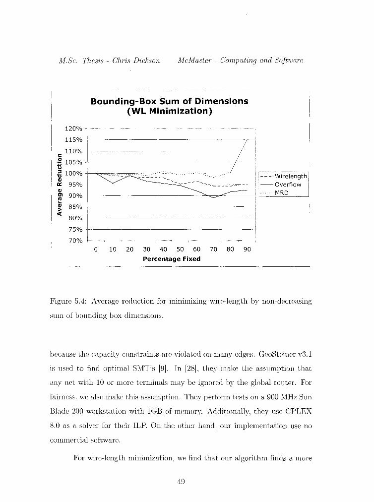
5.4 Average reduction for minimizing wire-length by non-decreasing
sum of bounding box dimensions. . . . . . . . . . . . . . . . . 49
Vll

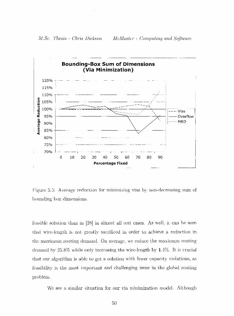
5.5 Average reduction for minimizing vias by non-decreasing sum
of bounding box dimensions. . . . . . . . . . . . . . . . . . . . 50
Vlll
List of Tables
1.1 Complexity of Disjktra's algorithm . . . . . . . 9
5.1 Comparison of tree generation times with and without path
saving heuristic. . . . . . . . . . . . . . . . . . . . . . . . . . . 44
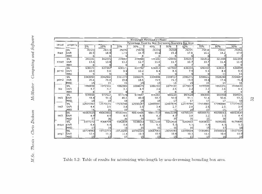
5.2 Table of results for minimi7,ing wire-length by non-decreasing
bounding box area. . . . . . . . . . . . . . . . . . . . . . . . . 52
5.3 Table of results for minimizing vias by non-decreasing bounding
box area. . . . . . . . . . . . . . . . . . . . . . . . . . . . . . . 53
5.4 Table of results for minimizing wire-length by non-decreasing
sum of bounding box dimensions. . . . . . . . . . . . . . . . . 54
5.5 Table of results for minimizing vias by non-decreasing sum of
bounding box dimensions. . . . . . . . . . . . . . . . . . 55
5.6 Wire-length minimization results for the test sets in [28] 56
5. 7 Via minimization results for the test sets in [28] . . . . . 56
IX

X
List of Algorithms
1
2
3
4
5
Dijkstra's algorithm for finding shortest paths.
Kruskal's algorithm for finding minimum spanning trees.
Prim's algorithm for finding minimum spanning trees. .
Approximation algorithm for global routing in VLSI design.
2-approximate Steiner tree algorithm [16]
Xl
7
11
13
26
30
Chapter 1
Introduction
It does not take an expert to see that the need and use of computers is rising.
They are used in almost every facet of industry. The quality of computing relies
heavily on the quality of the technology they are built upon. At the center of
all this is the demand for better integrated circuits. The rate at which these
circuits are growing in complexity is astonishing. The degree of integration
we use to measure a chip is the number of transistors contained within it.
Currently, we are working with circuits that contain millions of transistors.
It is estimated that, in the next decade, we will reach circuits that contain
billions of transistors [15]. Thus, the need for computer aided design (CAD)
tools to aid the circuit layout process is increasing rapidly.
VLSI circuit layout is the process by which the physical layout of a
circuit is realized from its functional description and specifications. This is
typically broken into multiple phases due to the increasing complexity of VLSI
circuits. Generally, we can break these phases into three main classes: parti
tioning, placement, and routing. In the partitioning phase, we split the area
of the chip into smaller, more manageable pieces. The assumption is that each
1
M.Sc. Thesis - Chris Dickson McMaster- Computing and Software
of these pieces may be designed independently. In the placement phase, we fix
the locations of all blocks within the chip, as well as produce a list of blocks
whose specific pins need to be connected with wire. In the routing phase, the
goal is to find a realization of the connections provided from the placement
phase. Typically, routing is broken into two distinct processes: global routing,
and detailed routing. In global routing, we wish to find an approximate in
terconnection between the blocks. Detailed routing takes the output from the
global router and produces the exact geometric layout of the wires to connect
the blocks.
1.1 Graph Theory
We begin with a brief introduction of graph theory. For all graphs and graph
algorithms in this chapter, see [1, 6] and references therein. A directed graph
G = (V, E) consists of a finite set of vertices V and a finite set E of edges
(arcs). An edge is an ordered pair of vertices ( u, v) where u, v E V. Often, an
edge ( u, v) is written as u -+ v. We say that an edge u -+ v is from u to v and
that v is adjacent to u. The degree of a vertex in an undirected graph is the
number of edges incident to it.
We can also define an undirected graph G = (V, E) where V is a finite set of
vertices and E is a finite set of undirected edges, i.e., in an undirected graph,
each edge is an unordered set of vertices. That is, if ( u, v) is an edge in G,
then ( v, u) is the same edge in G.
We define a weighted graph to be a graph (directed or undirected) with an
associated weight function w : E -+ ffi.. A path in a graph G = (V, E) from
2
M.Sc. Thesis - Chris Dickson McMaster- Computing and Software
vertex 'IL to vertex u' is a sequence of vertices (v0 , 'U1, .. . , vk), where v0 = 'IL
and vk = u' and (vi_ 1 , vi) E E fori= 1 ... k. The length of a path from u to
v/ is the length of the vertex sequence defining the path or 2:7=1 w( Vi-1, vi).
A path (v0 , v1 , ... , vk) forms a cycle if v0 = vk and the path contains at least
one edge. A graph that contains at least one cycle is called a cyclic graph. A
graph that contains no cycle is called acyclic. A graph is said to be planar if
it can be drawn in the plane such that its edges only intersect at vertices [4].
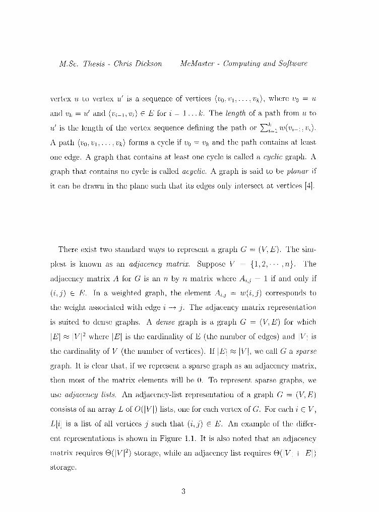
There exist two standard ways to represent a graph G = (V, E). The sim
plest is known as an adjacency matrix. Suppose V = { 1, 2, · · · , n}. The
adjacency matrix A for G is an n by n matrix where Ai,j = 1 if and only if
(i,j) E E. In a weighted graph, the element A,j = w(i,j) corresponds to
the weight associated with edge i -+ j. The adjacency matrix representation
is suited to dense graphs. A dense graph is a graph G = (V, E) for which
lEI ~ IVI 2 where lEI is the cardinality of E (the number of edges) and lVI is
the cardinality of V (the number of vertices). If lEI ~ lVI, we call G a sparse
graph. It is clear that, if we represent a sparse graph as an adjacency matrix,
then most of the matrix elements will be 0. To represent sparse graphs, we
use adjacency lists. An adjacency-list representation of a graph G = (V, E)
consists of an array L of O(IVI) lists, one for each vertex of G. For each i E V,
L[i] is a list of all vertices j such that ( i, ,j) E E. An example of the differ
ent representations is shown in Figure 1.1. It is also noted that an adjacency
matrix requires 8(IVI 2) storage, while an adjacency list requires 8(1VI +lEI)
storage.
3
M.Sc. Thesis - Chris Dickson McMaster- Computing and Software
(a) A graph G
(b) Adjacency list repre
sentation of G
0 1 1 0 0 0 0 1 0
(c) Adjacency matrix rep
resentation of G
Figure 1.1: A graph is shown along with its different data structures used to
represent it.
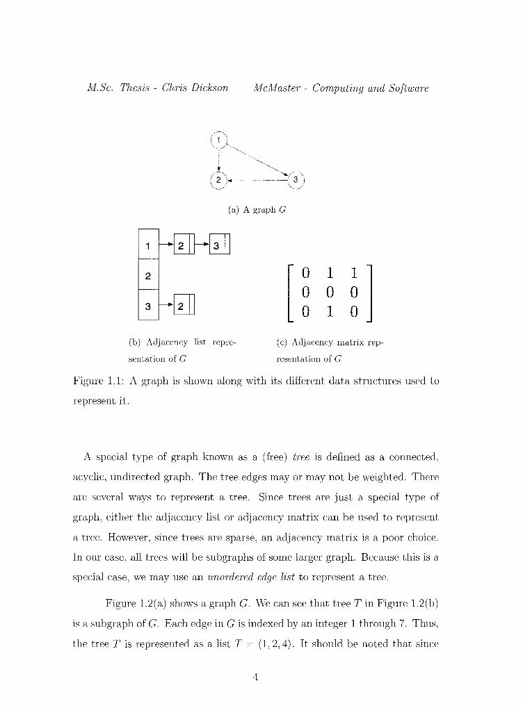
A special type of graph known as a (free) tree is defined as a connected,
acyclic, undirected graph. The tree edges may or may not be weighted. There
are several ways to represent a tree. Since trees are just a special type of
graph, either the adjacency list or adjacency matrix can be used to represent
a tree. However, since trees are sparse, an adjacency matrix is a poor choice.
In our case, all trees will be subgraphs of some larger graph. Because this is a
special case, we may use an unordered edge list to represent a tree.
Figure 1.2(a) shows a graph G. We can see that tree Tin Figure 1.2(b)
is a subgraph of G. Each edge in G is indexed by an integer 1 through 7. Thus,
the tree Tis represented as a list T = (1, 2, 4). It should be noted that since
4
M.Sc. Thesis - Chris Dickson McMaster- Computing and Software
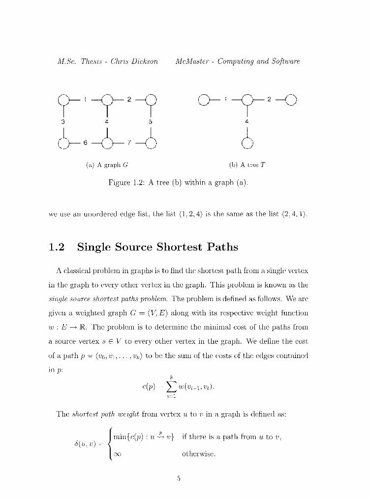
(a) A graph G (b) A tree T
Figure 1.2: A tree (b) within a graph (a).
we use an unordered edge list, the list \1, 2, 4) is the same as the list \2, 4, 1).
1.2 Single Source Shortest Paths
A classical problem in graphs is to find the shortest path from a single vertex
in the graph to every other vertex in the graph. This problem is known as the
single source shortest paths pmblem. The problem is defined as follows. We arc
given a weighted graph G = (V, E) along with its respective weight function
w : E --+ R The problem is to determine the minimal cost of the paths from
a source vertex s E V to every other vertex in the graph. We define the cost
of a path p = \v0, 'lh, ... , vk) to be the sum of the costs of the edges contained
lil p: k
c(p) = L w(vi-l, vi)· i=l
The shortest path weight from vertex 'U to v in a graph is defined as:
{
min { c(p) : 'U !;, v} if there is a path from u to v, 6(u,v)=
oo otherwise.
5
M.Sc. Thesis - Chris Dickson McMaster- Computing and Software
Thus, the shortest path from vertex u to vertex v IS any path p
(u, ... ,v), where c(p) = 6(u,v).
The best known method for solving the single source shortest paths prob
lem in graphs is by an algorithm presented by Dijkstra in 1959 [7]. This is
a classical example of a greedy algorithm in that making a locally optimal
(greedy) choice leads to a globally optimal solution. This is not always true
for greedy algorithms, but as it turns out, Dijkstra's algorithm always gives
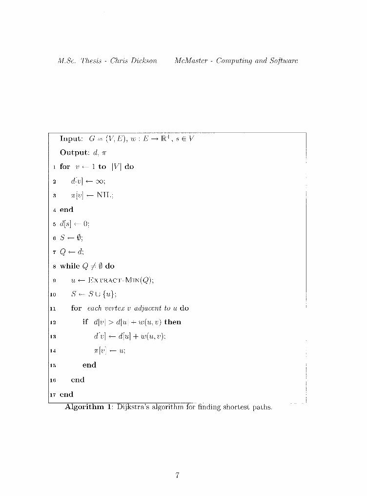
the optimal solution, if it exists. The pseudocode for Dijkstra's algorithm is
given in Algorithm 1.
The input consists of a weighted graph G = (V, E) along its respective weight
function w. Dijkstra's algorithm requires that no edge in G have negative
weight. However, free edges or edges with weight 0 are allowed. We must also
specify a source verex s. This is the vertex for which we wish to compute the
shortest paths from.
The algorithm works by maintaining a set of unvisited vertices along with the
shortest distance so far from the source to all vertices. The aforementioned set
is defined by S and the distances are stored in the array d. At each iteration,
we select an unvisited vertex u whose distance from the source is minimal. This
is achieved by storing the distance estimates in a min-priority queue. We then
check each vertex v adjacent to u to see if going through vertex v can improve
the shortest path estimate. This step is known as relaxation. Additionally, if
we wish to reconstruct the shortest paths, we must store an additional array,
7f, that records the parent of each vertex in the shortest path.
6
M.Sc. Thesis - Chris Dickson McMaster- Computing and Software
Input: G = (V, E), w: E ~ ffi.+, s E V
Output: d, 1r
1 for v +-- 1 to IV I do
2 d[v] +-- oo;
3 1r[v] +-- NIL;
4 end
5 d[s] +-- 0;
6 sf- 0;
7 Q f- d;
8 while Q f 0 do
9 u +-- EXTRACT-MIN(Q);
10 sf- s u { u };
11 for each vertex v a~jacent to u do
12 if d[v] > d[u] + w(u, v) then
13 d[v] +-- d[u] + w(u, v);
14 1r[v] +-- 'u;
15 end
16 end
11 end
Algorithm 1: Dijkstra's algorithm for finding shortest paths.
7
M.Sc. Thesis - Chris Dickson McMaster- Computing and Software
Theorem 1.1. {6} If we are given a graph G = (V, E) along with a nonnegative
weight function w and a source vertex s E V, then running D~jkstra 's algorithm
will terminate with d[v] = 6(s, v) for all vertices v E V.
When Disjktra first presented this algorithm, he made no mention of using
a priority queue to find the minimum distance estimate. However, as we
will soon see, the choice of queue drastically affects the performance of this
algorithm. Lines 1 through 7 are used to perform initialization. We set the
distance estimates to infinity for all vertices except the source vertex s. This
is to ensure that the source vertex is the first vertex we pick in the main loop.
Additionally, we initialize the array of parent pointers to NIL and the set S
of visited vertices to empty. Line 7 initializes a priority queue Q to contain
the distance estimates found in d. Lines 8 through 17 make up the main
loop of the algorithm. Line 9 finds the next unvisited vertex by extracting
the minimum element from the priority queue. Line 10 marks the vertex as
visited. Line 11 through 16 perform the so-called relaxation procedure. The
overall running time of the algorithm depends on the choice of priority queue
used to implement Q. In general we give the following theorem.
Theorem 1.2. {6} The complexity of Dijkstra's algorithm is 8(1VI)·TExTRAcT-MrN+
8(IEI) ·TDEcnEA~E-KEv where TExTRAcT-MrN and TDEcRroAsE-KEY are the running times
for the EXTRACT-MIN and DECREASE-KEY procedures respectively for any
implementation of a priority queue.
Proof. For a proof, see [ 6]. D
We summarize in Table 1.1 the overall complexity of Dijkstra's algo
rithm with various priority queues.
8
M.Sc. Thesis - Chris Dickson McMaster- Computing and Software
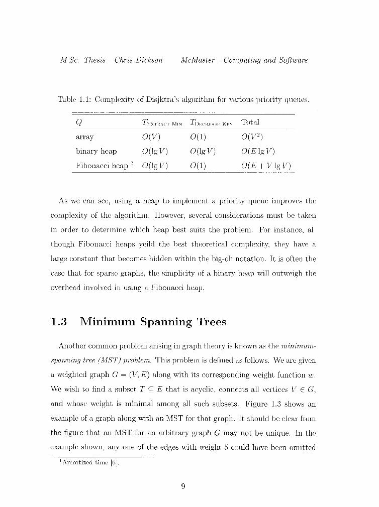
Table 1.1: Complexity of Disjktra's algorithm for various priority queues.
Q TEXTHACT-MIN TDECREASE-KEY Total
array O(V) 0(1) O(V2)
binary heap O(lg V) O(lg V) O(E lg V)
Fibonacci heap 1 O(lg V) 0(1) O(E+VlgV)
As we can see, using a heap to implement a priority queue improves the
complexity of the algorithm. However, several considerations must be taken
in order to determine which heap best suits the problem. For instance, al
though Fibonacci heaps yeild the best theoretical complexity, they have a
large constant that becomes hidden within the big-oh notation. It is often the
case that for sparse graphs, the simplicity of a binary heap will outweigh the
overhead involved in using a Fibonacci heap.
1.3 Minimum Spanning 'frees
Another common problem arising in graph theory is known as the minimum
spanning tree (MST) pmblem. This problem is defined as follows. We are given
a weighted graph G = (V, E) along with its corresponding weight function w.
We wish to find a subset T <;;;; E that is acyclic, connects all vertices V E G,
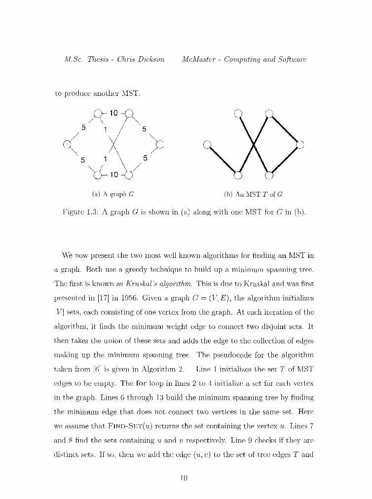
and whose weight is minimal among all such subsets. Figure 1.3 shows an
example of a graph along with an MST for that graph. It should be clear from
the figure that an MST for an arbitrary graph G may not be unique. In the
example shown, any one of the edges with weight 5 could have been omitted
1Amortized time [6].
9
M. Sc. Thesis - Chris Dickson McMaster- Computing and Software
to produce another MST.
10
5 1 5
( --5 1 5
(a) A graph G (b) An MST T of G
Figure 1.3: A graph G is shown in (a) along with one MST for Gin (b).
We now present the two most well known algorithms for finding an MST in
a graph. Both use a greedy technique to build up a minimum spanning tree.
The first is known as Kruskal's algorithm. This is due to Kruskal and was first
presented in [17] in 1956. Given a graph G = (V, E), the algorithm initializes
lVI sets, each consisting of one vertex from the graph. At each iteration of the
algorithm, it finds the minimum weight edge to connect two disjoint sets. It
then takes the union of these sets and adds the edge to the collection of edges
making up the minimum spanning tree. The pseudocode for the algorithm
taken from [6] is given in Algorithm 2. Line 1 initializes the set T of MST
edges to be empty. The for loop in lines 2 to 4 initialize a set for each vertex
in the graph. Lines 6 through 13 build the minimum spanning tree by finding
the minimum edge that does not connect two vertices in the same set. Here
we assume that FIND-SET( u) returns the set containing the vertex u. Lines 7
and 8 find the sets containing u and v respectively. Line 9 checks if they are
distinct sets. If so, then we add the edge ( u, v) to the set of tree edges T and
10
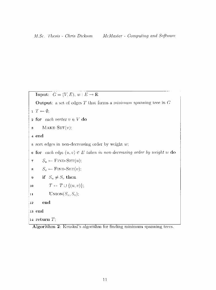
M.Sc. Thesis - Chris Dickson McMaster- Computing and Software
Input: G = (V, E), w: E---+ lR
Output: a set of edges T that forms a minimum spanning tree in G
1 T +-- 0;
2 for each vertex v E V do
3 MAKE-8ET(v);
4 end
5 sort edges in non-decreasing order by weight w;
6 for each edge ( 1L, v) E E taken in non-decreasing order by weight w do
7 S11 +-- FIND-8ET(u);
8 Sv +-- FIND-SET(v);
9 if Su -::1 Sv then
10 T +-- T U {(v,, v)};
11 UNION(Su, Sv);
12 end
13 end
14 return T;
Algorithm 2: Kruskal's algorithm for finding minimum spanning trees.
11
M.Sc. Thesis - Chris Dickson McMaster- Computing and Software
perform the union of the sets containing u and v.
Theorem 1.3. (6} If we are given a graph G = (V, E) and a weight function
w, then Tunning Kruskal's algorithm will find one minimum spanning tree T
in G.
We must now analyze the running time of Kruskal's algorithm. Us
ing the disjoint set implementation described in [6], the overall complexity
of Kruskal's algorithm is O(IEilg lEI). If we have a sparse graph where
lEI = O(lg lVI), then the complexity is improved to O(IEilg lVI).
One drawback of implementing Kruskal's algorithm is that it requires
a good implementation of a relatively complex data structure for disjoint sets.
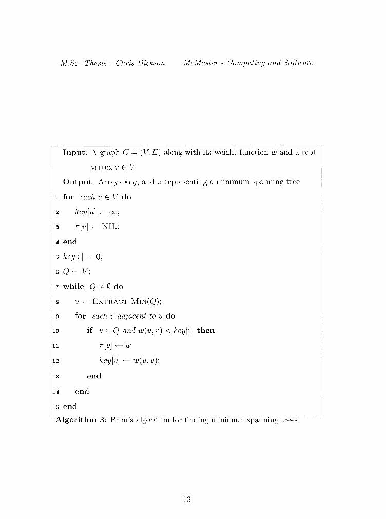
Another algorithm known as Prim's algorithm [22] does not require such a
complex data structure. Prim's algorithm also finds a minimum spanning tree
in a graph G and is given in Algorithm 3. The pseudocode for this algorithm
is taken from [6].
Prim's algorithm works by maintaining a set Q of vertices not yet en
countered. Each time it removes a vertex v from Q, it checks if the weight of
each edge incident upon u is less than the key value for the vertices adjacent
to u. This is very similiar to the way that Dijkstra's algorithm finds short
est paths. Similar to Dijkstra's algorithm, we must also use a min-priority
queue to store the key values of the vertices. The running time of Prim's al
gorithm depends on the choice of min-priority queue. If a binary heap is used
to implement the min-priority queue, the running time of Prim's algorithm is
O(IEilog lVI).
12
M.Sc. Thesis - Chris Dickson McMaster- Computing and Software
Input: A graph G = (V, E) along with its weight function w and a root
vertex rEV
Output: Arrays key, and 1r representing a minimum spanning tree
1 for each u E V do
2 key[v,] +- oo;
3 1r[u] +- NIL;
4 end
5 key[r] +- 0;
6 Q +- V;
7 while Q =/= 0 do
8 u +- EXTRACT-MIN(Q);
g for each v adjacent to u do
10 if v E Q and w(u, v) < key[v] then
11 1r[v] +- u;
12 key[v] +- w(u, v);
13 end
14 end
15 end
Algorithm 3: Prim's algorithm for finding minimum spanning trees.
13
M.Sc. Thesis - Chris Dickson McMaster- Computing and Software
1.4 Approximation Algorithms
An approximation algorithm for a minimization problem is an algorithm
that returns a near optimal solution in polynomial time. We say that an
approximation algorithm has an approximation ratio of r if the ratio of the
objective value produced by the algorithm and the optimal objective value
is less than or equal to r [6]. Furthermore, we call an algorithm with an
approximation ratio of r an /-approximation algorithm.
A polynomial time approximation scheme (PTAS) is an algorithm such
that for any fixed E > 0, we obtain a (1 +E)-approximation algorithm.
1.5 Steiner Minimal Trees
The Steiner minimal tree problem is a problem arising in graph theory that
can be defined as follows. Given a weighted graph G = (V, E) and a set of
vertices S s;;; V, find a minimum weight connected subgraph of G that includes
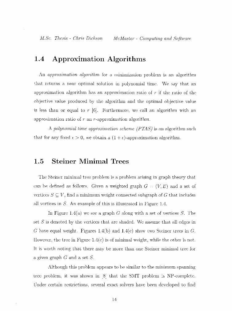
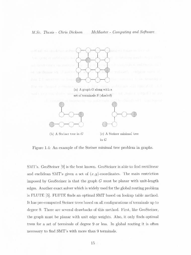
all vertices in S. An example of this is illustrated in Figure 1.4.
In Figure 1.4( a) we see a graph G along with a set of vertices S. The
set S is denoted by the vertices that are shaded. We assume that all edges in
G have equal weight. Figures 1.4(b) and 1.4( c) show two Steiner trees in G.
However, the tree in Figure 1.4( c) is of minimal weight, while the other is not.
It is worth noting that there may be more than one Steiner minimal tree for
a given graph G and a set S.
Although this problem appears to be similar to the minimum spanning
tree problem, it was shown in [8] that the SMT problem is NP-complete.
Under certain restrictions, several exact solvers have been developed to find
14
NJ.Sc. Thesis - Chris Dickson McMaster- Computing and Software
(a) A graph G along wit h a
set of terminals S (shaded)
(b) A Steiner t ree in G (c) A Steiner minimal tree
in G
Figure 1.4: An example of the Steiner minimal tree problem in graphs.
SMT's. GeoSteiner [9] is the best known. GeoSteiner is able to find rectilinear
and euclidean SMT's given a set of (x, y)-coordinates. The main restriction
imposed by GeoSteiner is that t he graph G must be planar with unit-length
edges. Another exact solver which is widely used for the global routing problem
is FLUTE [5]. FLUTE finds an optimal SMT based on lookup t able method.
It has pre-computed Steiner trees based on all configurations of terminals up to
degree 9. There are several drawbacks of this method . First , like GeoSteiner ,
the graph must be planar with unit edge weights. Also, it only finds optimal
t rees for a set of t erminals of degree 9 or less . In global routing it is often
necessary to find SMT's with more than 9 t erminals.
15
M.Sc. Thesis - Chris Dickson McMaster- Computing and Software
As well as exact techniques, several approximation methods for finding
SMT's have been presented. In [16] a 2-approximation algorithm is proposed.
This algorithm is designed for general graphs, and imposes no restrictions on
the edge weights. Another advantage of this algorithm is its simplicity to
implement as it requires only the algorithms discussed in Sections 1.2 and
1.3. Although this algorithm comes with a 2-approximation bound, we will
see in Chapter 5 that, for our case, it delivers solutions which are very close
to optimal. The details of this algorithm are presented in Chapter 3.
16
Chapter 2
Mathematical Formulation
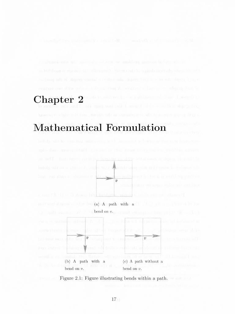
(a) A path with a
bend on v.
(b) A path with a
bend on v.
(c) A path without a
bend on v .
Figure 2.1: Figure illustrating bends within a path .
17
M.Sc. Thesis - Chris Dickson McMaster- Computing and Software
In the global routing problem, we aim to minimize the wire-length for
the ultimate physical design of the circuit. Generally, the circuit is modeled as
a grid graph. An m x n grid graph, also called a lattice graph, is the product
of path graphs on m and n vertices. A path graph is a tree with two vertices
of degree 1, and the remaining n- 2 vertices of degree 2. An example of a
grid graph is illustrated in Figure 1.4(a) (see page 15). Thus, the vertices of
a grid graph represent the components in the circuit, and the edges represent
the routing channels or the areas in which wire may be placed. A set of
vertices which need to be connected with wire is known as a net. Each vertex
contained in a net is called a terminal. In a particular instance of the global
routing problem, we are given many nets to connect. Furthermore, each edge
of the grid graph is associated with an integral capacity constraint. That is,
the number of wires that may pass through that edge. A solution to the global
routing problem is a set of trees that connects the terminals of each net, and
satisfies the edge capacity constraints.
Formally, we are given a planar, weighted grid graph G = (V, E) and a
set of nets S1 , ... , SK ~ V. The edge set is associated with a length function
l: E----+ JR.+ U {0} and a capacity function c: E----+ JR.+ 2. We assume that ISkl
is bounded by some constant for all k = 1, ... , K. A feasible solution is a set
of K trees spanning S1 , ... , SK with respect to the edge capacity constraints.
The overall cost of the solution consists of two parts: (i) the edge cost and (ii)
the total number of bends in the trees called the bend-dependent vertex cost
(see Figure 2.1). The goal is to minimize the overall cost defined as a linear
combination altotal + f)vtotal, where ltotal is the sum of edge length of all K
2 Although we arc physically restricted to having integral edge capacities, for the presen
tation of the algorithm we allow fractional capacities.
18
M.Sc. Thesis - Chris Dickson McMaster- Computing and Software
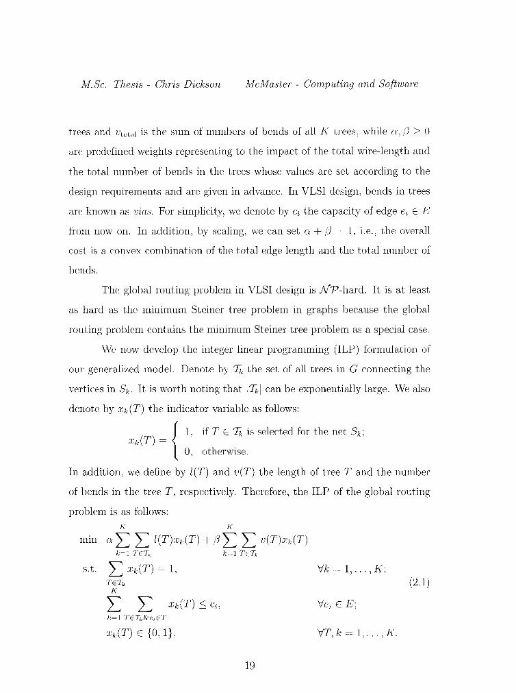
trees and Vtotal is the sum of numbers of bends of all K trees, while o:, /3 ~ 0
are predefined weights representing to the impact of the total wire-length and
the total number of bends in the trees whose values are set according to the
design requirements and are given in advance. In VLSI design, bends in trees
are known as vias. For simplicity, we denote by ci the capacity of edge ei E E
from now on. In addition, by scaling, we can set a+ /3 = 1, i.e., the overall
cost is a convex combination of the total edge length and the total number of
bends.
The global routing problem in VLSI design is NP-hard. It is at least
as hard as the minimum Steiner tree problem in graphs because the global
routing problem contains the minimum Steiner tree problem as a special case.
We now develop the integer linear programming (ILP) formulation of
our generalized model. Denote by '4 the set of all trees in G connecting the
vertices in Sk. It is worth noting that 1'41 can be exponentially large. We also
denote by xk(T) the indicator variable as follows:
{
1, if T E '4 is selected for the net Sk; Xk(T) =
0, otherwise.
In addition, we define by l(T) and v(T) the length of tree T and the number
of bends in the tree T, respectively. Therefore, the ILP of the global routing
problem is as follows:
K K
rmn a L L l(T)xk(T) + /3 L L v(T)xk(T) k=l TETk k=l TET,.
s.t. L xk(T) = 1, Vk = 1, ... ,K; TETk (2.1)
K
2..: 2::: xk(T) Sci, \lei E E; k=l TET,.,&eiET
xk(T) E {0, 1}, \IT, k = 1, ... , K.
19
M.Sc. Thesis - Chris Dickson McMaster- Computing and Software
The third set of constraints enforce that the value of x for each tree be either
0 or 1. This implies that the first set of constraints enforces that exactly one
tree is chosen to route the net Sk. The second set of constraints are capacity
constraints for the edges.
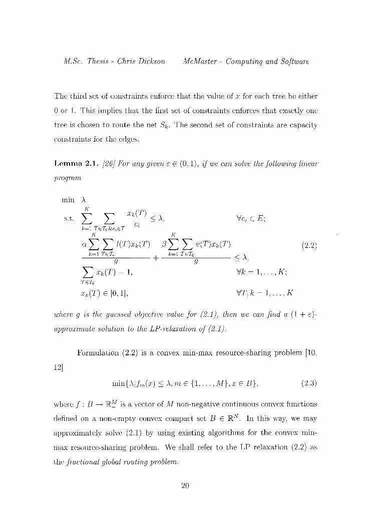
Lemma 2.1. (26} For any given f E (0, 1), if we can solve the following linear
program
mm A.
s.t. K
I: k=l TE~,&e;ET
K
Xk(T) --<A.
- ' C· 1.
K
a L L l(T)xk(T) j3 L L v(T)xk(T) k=l TETk k=l TETk < \ ___ ___:::.,g:----- + ___ ___:::.,g=----- - A,
L .Tk (T) = 1' 'Ilk = 1' ... ' K; TETk
Xk(T) E [0, 1], VT,k=1, ... ,K
(2.2)
where g is the guessed objective value for (2.1), then we can find a (1 +c)
approximate solution to the LP-relaxation of (2.1).
Formulation (2.2) is a convex min-max resource-sharing problem [10,
12]
min{A.!.fm(x) ~A., mE {1, ... , M}, x E B}, (2.3)
where f : B ---+ IR~ is a vector of M non-negative continuous convex functions
defined on a non-empty convex compact set B E IRN. In this way, we may
approximately solve (2.1) by using existing algorithms for the convex min
max resource-sharing problem. We shall refer to the LP relaxation (2.2) as
the fractional global routing problem.
20
M.Sc. Thesis - Chris Dickson McMaster- Computing and Software
Since I'Ik I may be exponentially large, many exact algorithms for LPs
such as standard interior point methods cannot be applied to obtain a polyno
mial time algorithm. It is possible to solve such a problem by the volumetric
center [2] or the ellipsoid methods with separation oracle [11]. However, those
approaches will lead to a large running time, which is unsuitable for global
routing, as instances of these problems are typically too large.
We will apply the approximation algorithm £ in [13] for convex min
max resource-sharing problems. Algorithm 4 (see page 26) is a specialization
of£ for the global routing problem. By applying this algorithm, we avoid the
exponential size of T. In £, we generate K minimum Steiner trees for the
K nets in each iteration. Thus, there is only a polynomial number of Steiner
trees generated in total. In fact, it is shown in [26] that the approximation
algorithm generates at most O(Km(logm+c:-2 logc:-1)) Steiner trees, where
m is the number of edges in the grid graph, and the following result for the
fractional global routing holds:
Theorem 2.1. Algorithm 4 is an r(1 + c:)-appmxirnation algorithm for the
fractional global muting pmblem (2.2) pmvided that an r-approximate mini
mum Steiner tree solver is available.
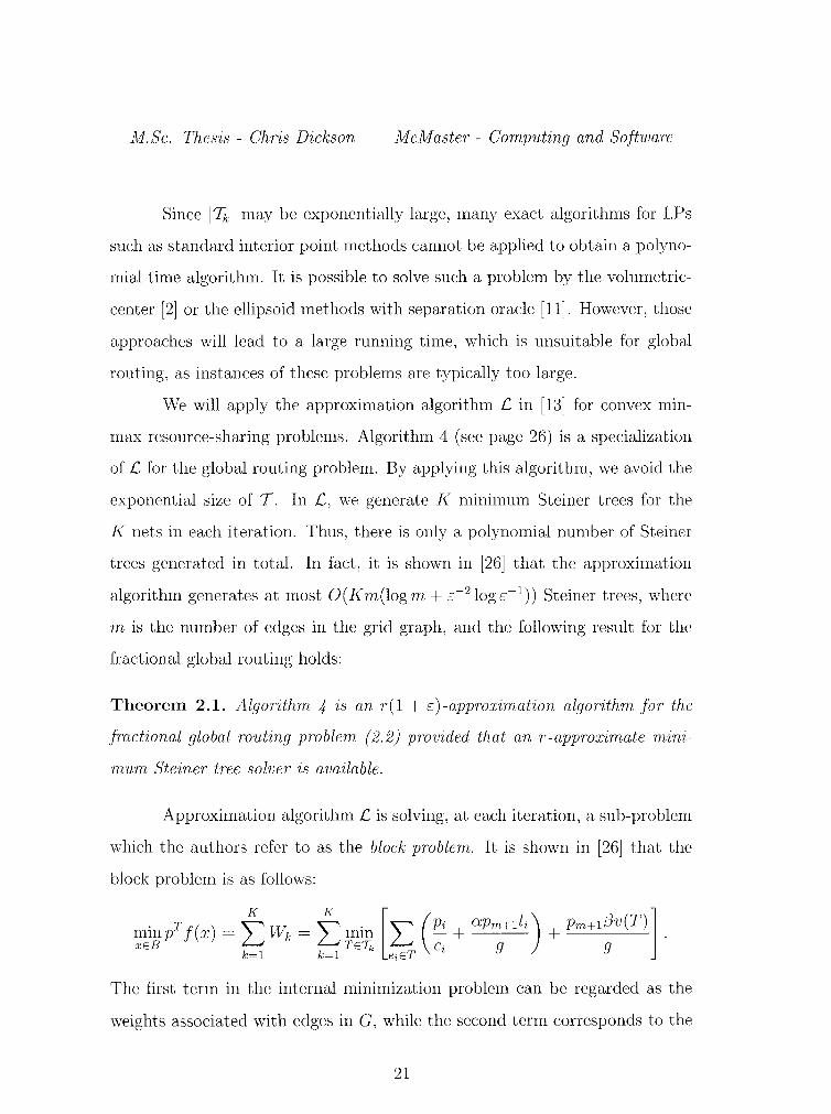
Approximation algorithm£ is solving, at each iteration, a sub-problem
which the authors refer to as the block problem. It is shown in [26] that the
block problem is as follows:
. rf( ) ~ W ~ . [~. (Pi+ O!Pm+lli) + Pm+lf3v(T)l mm p x = L.....t k = 6 mm L.....t - . xEB TETk Ci g g
k=l k=l eiET .
The first term in the internal minimization problem can be regarded as the
weights associated with edges in G, while the second term corresponds to the
21
M.Sc. Thesis - Chris Dickson
( y
v
X
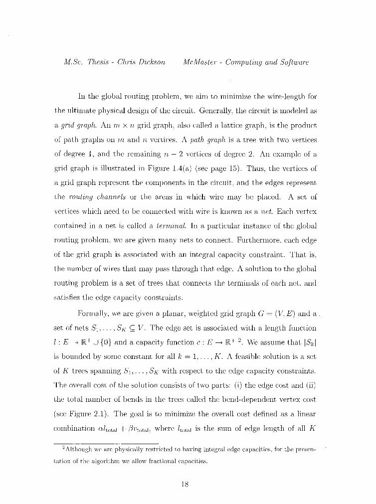
Figure 2.2: Original grid graph
G.
z j
McMaster- Computing and Software
v'
v
- X
Figure 2.3 : Virtual layer graph H.
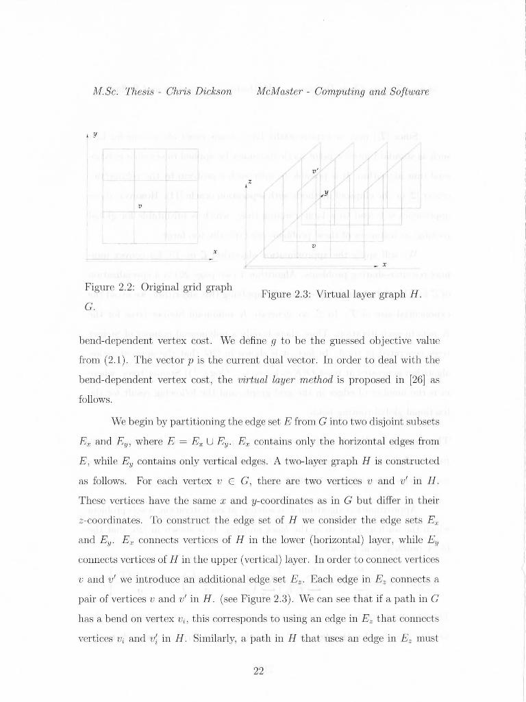
bend-dependent vertex cost . We define g to be the guessed object ive value
from (2.1 ). The vector p is the current dual vector. In order to deal with the
bend-dependent vertex cost , the virtual layer m ethod is proposed in [26] as
follows.
We begin by part it ioning the edge set E from G into two disjoint subsets
Ex and Ey, where E = Ex U Ey. Ex contains only the horizontal edges from
E, while Ey contains only vertical edges . A two-layer graph H is constructed
as fo llows. For each vertex v E G , there are two vertices v and v' in H .
These vertices have the same x and y-coordinates as in G but differ in their
z-coordinates . To construct the edge set of H we consider the edg sets Ex
and Ey. Ex connects vertices of H in the lower (horizontal) lay r , while Ey
connect s vertices of H in the upper (verti cal) layer. In order to connect vertices
v and v' we introduce an additional edge set Ez. Each edge in Ez connects a
pair of vert ices v and v' in H. (see Figure 2.3). vVe can see that if a path in G
has a bend on vertex vi , t his corresponds to using an edge in Ez that connects
vert ices vi and v~ in H . Similarly, a path in H that uses an edge in Ez must
22
M.Sc. Thesis - Chris Dickson McMaster- Computing and Software
have a bend on its corresponding path in G.
We now set the weights to the edges in H. For any edge ei E Ex U Ey,
we assign a weight wi = pi/ ci + O:Pm+ 1ld g according to their indices in the
original graph G. For every edge inEz, we assign a weight Pm+ 1(3jg. In this
weighted, two-layer graph H, a minimum Steiner tree for a net Sk corresponds
to a tree for Sk in G with the minimum Wk. So when we apply Algorithm
£, the block problem corresponds to the classical Steiner tree problem in the
graph H to minimize the overall edge weight of the Steiner tree connecting
the vertices in Sk. We can apply an approximate solver for the Steiner tree
problem as the block solver of Algorithm £.
Once we have a fractional solution given by the approximation algo
rithm £, we must round it to find a feasible integer solution. In addition,
we must have a performance guarantee of the approximation ratio. We use
randomized rounding (see Section 3.3) as described in [24, 23]. Algorithm 4
on page 26 summarizes the afformentioned method. For that algorithm, the
following theorem holds:
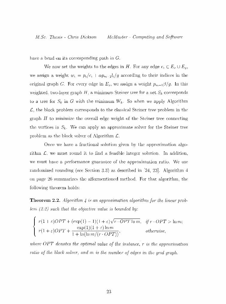
Theorem 2.2. Algorithm 4 is an approximation algorithm for the linear prob
lem (2.2) sv.ch that the objective value is bounded by:
{
r ( 1 + c) 0 PT + ( exp ( 1) - 1) ( 1 + c) J r · 0 PT ln m,
r( 1 + c)OPT + exp(1)(1 +c) ln m , 1 + ln(ln m/(r ·OPT))
ifr ·OPT> lnm;
otherwise,
where OPT denotes the optimal value of the instance, r is the approximation
ratio of the block solver, and m is the number of edges in the grid graph.
23

M.Sc. Thesis - Chris Dickson McMaster- Computing and Software
24
Chapter 3
Implementation
In this chapter, we present an implementation of the approximation algorithm
in [26] for the ILP formulation of the global routing problem in VLSI design.
We first present a basic outline of this algorithm, then go into some details
about the methods for Steiner tree approximation, as well as rounding approx
imate solutions to the ILP formulation.
3.1 Outline
We now present a basic outline of the approximation algorithm used to solve
the LP (2.2) in Chapter 2. We outline this in Algorithm 4.
Our input is given as a grid graph G = (V, E). Usually, this is sim
plified to two integers corresponding to the length and the width of graph
G. Additionally, we may be given a list of missing vertices (holes) and/or an
edge length function. If no edge lengths are specified, then they are assumed
to be of unit-length, i.e., length one. We are also given a non-empty set of
nets. Each net Sk is a set of vertices (coordinates) in G, where ISkl ~ 2 for
25
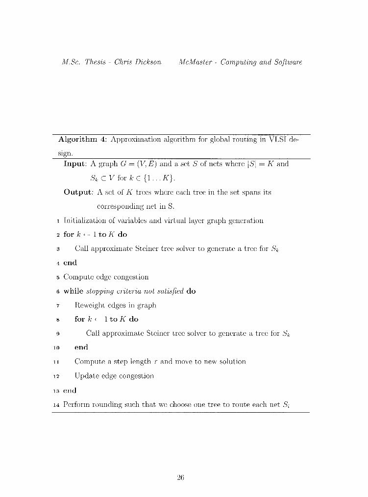
M. Sc. Thesis - Chris Dickson McMaster- Computing and Software
Algorithm 4: Approximation algorithm for global routing in VLSI de-
s1gn.
Input: A graph G = (V, E) and a setS of nets where lSI = K and
Sk c V fork E {1 ... K}.
Output: A set of K trees where each tree in the set spans its
corresponding net in S.
1 Initialization of variables and virtual layer graph generation
2 for k +- 1 to K do
3 Call approximate Steiner tree solver to generate a tree for Sk
4 end
5 Compute edge congestion
6 while stopping criteria not satisfied do
1 Reweight edges in graph
s for k +- 1 to K do
9 Call approximate Steiner tree solver to generate a tree for Sk
10 end
11 Compute a step length T and move to new solution
12 Update edge congestion
13 end
14 Perform rounding such that we choose one tree to route each net Si
26
M.Sc. Thesis - ChTis Dickson McMasteT- Computing and SoftwaTe
kE{1 ... K}.
Line 1 involves initializing local variables as well as transforming the
grid graph G into a viTtual layeT gmph which will be denoted as H. In lines
2 - 4 we generate a tree for each net in S. To achieve this, we simply call
our approximate Steiner tree solver which will generate a tree when given the
graph Hand a net Sk. In line 5 we compute the edge congestion for each edge
in G. The edge congestion for the edge ei is equal to the number of trees that
pass through it.
We now enter the main loop of our algorithm. Line 7 reweights the
edges in our virtual layer graph. The edge weights are chosen such that highly
congested edges will have a larger weight in H than those edges that are less
congested. In this way, when we compute the next set of trees in lines 8- 10,
the edges that are frequently used in previous iterations will be avoided. In
line 11 we compute a step length T E (0, 1] for the current iteration. This step
length can be thought of as a measure of "goodness" for the current iteration.
The details of computing the step length are discussed in Section 4.
After each iteration of the main loop (lines 6 through 13), we compute
the congestion for each edge ei. However, since we keep the trees generated
in previous iterations, we must measure how often each edge is used in all
iterations. Without loss of generality, the edge congestion for an edge ei can
be scaled by its capacity such that it is a non-negative real number. We will
denote this scaled congestion as k Formally, fi = nd ci where n; is the number
of edge crossing edge ei and ci is the capacity. A value of fi that is strictly
greater than 1 implies that this edge is over capacity. This leads to the concept
of fmctional edge congestion. We compute the new fractional edge congestion
27
M.Sc. Thesis - Chris Dickson McMaster- Computing and Software
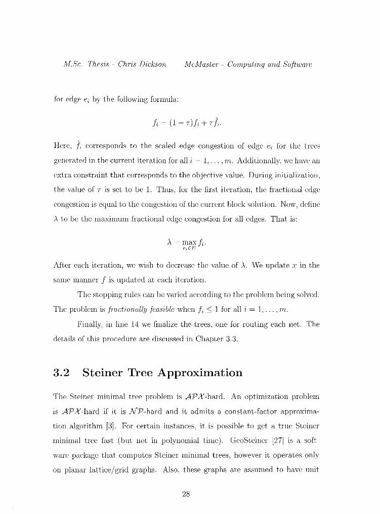
for edge ei by the following formula:
Here, fi corresponds to the scaled edge congestion of edge ei for the trees
generated in the current iteration for all i = 1, ... , m. Additionally, we have an
extra constraint that corresponds to the objective value. During initialization,
the value of T is set to be 1. Thus, for the first iteration, the fractional edge
congestion is equal to the congestion ofthe current block solution. Now, define
A to be the maximum fractional edge congestion for all edges. That is:
A= maxfi· e;EE
After each iteration, we wish to decrease the value of A. We update x in the
same manner f is updated at each iteration.
The stopping rules can be varied according to the problem being solved.
The problem is fractionally feasible when fi :::;: 1 for all i = 1, ... , m.
Finally, in line 14 we finalize the trees, one for routing each net. The
details of this procedure are discussed in Chapter 3.3.
3.2 Steiner Tree Approximation
The Steiner minimal tree problem is AP X-hard. An optimization problem
is APX-hard if it is NP-hard and it admits a constant-factor approxima
tion algorithm [3]. For certain instances, it is possible to get a true Steiner
minimal tree fast (but not in polynomial time). GeoSteiner [27] is a soft-
ware package that computes Steiner minimal trees, however it operates only
on planar lattice/grid graphs. Also, these graphs are assumed to have unit
28
M.Sc. Thesis - Chris Dickson McMaster- Computing and Software
length. Although the edge lengths in our grid graph may have unit length,
the edge weights in the virtual layer graph may not have unit length. Thus,
this package is unsuitable in our algorithm. Additionally, GeoSteiner does not
run in polynomial time in the worst case. From now on, the notion of Steiner
minimal trees will be abbreviated as SMT and the abbreviation MST refers to
the minimum spanning tree problem.
There are many known approximation algorithms for computing SMT's,
where some have performance guarantees or approximation ratios while oth
ers do not. We will discuss only those with an approximation ratio, as this is
needed to provide a performance guarantee for our overall algorithm. A simple
2-approximation algorithm was presented in [16]. Robins and Zelikovsky [25]
developed a !.55-approximation method, implementations of which exist, but
yield large running times which is unsuitable for our applications. The best
known lower bound of the approximation ratio is ~~ [14]. It should be noted
that there is no polynomial time approximation algorithm that guarantees this
ratio.
We choose to use the 2-approximation algorithm introduced in [16] due
to its simplicity and low running time as well as its theoretical performance.
Computation results indicate that for our application, the approximation ratio
is very close to one. The pseudo-code for this approximation algorithm is
presented in Algorithm 5.
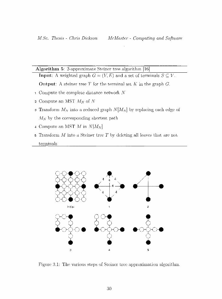
An example of this algorithm is illustrated in Figure 3.1. The computa
tional bottleneck of this algorithm is the computation of the complete distance
network. The complete distance network is the shortest distance between all
pairs of terminals in the net. We use Dijkstra's algorithm with a binary heap
as priority queue in order to achieve a complexity of O(IEilog lVI). There are
29
M.Sc. Thesis - Chris Dickson McMaster- Computing and Software
Algorithm 5: 2-approximate Steiner tree algorithm [16]
Input: A weighted graph G = (V, E) and a set of terminals S ~ V.
Output: A steiner tree T for the terminal set K in the graph G.
1 Compute the complete distance network N
2 Compute an MST MN of N
3 Transform MN into a reduced graph N[MN] by replacing each edge of
MN by the corresponding shortest path
4 Compute an MST M in N[MN]
5 Transform M into a Steiner tree T by deleting all leaves that are not
terminals
Initial 2
3 4 5
Figure 3.1: The various steps of Steiner tree approximation algorithm.
30
M.Sc. Thesis - Chris Dickson McMaster- Comput·ing and Software
other advanced data structures such a Fibonacci heaps or pairing heaps which
give a better theoretical complexity result. However, these heaps require sig
nificant overhead and only have better performance in the case of vertices with
high degree (dense graphs), while our underlying graphs are sparse. We use
a O(IVI 2) version of Prim's algorithm to compute minimum spanning trees.
It should be noted that the graphs in which we run Prim's algorithm have
significantly less vertices than the original graph, so we would not expect to
see a big improvement in running time even if we used an MST algorithm with
a better time complexity.
Additional improvements have been made to this algorithm that not
only improve the running time but also the quality of the solution. These are
discussed in Chapter 4.
3.3 Rounding
We implement randomized rounding [24, 23] in order to obtain an integer
solution from our fractional solution. Assume that we perform a total of p
iterations while solving the LP (2.2) in Chapter 2. We know that for each
net Sk we will have a total of p + 1 Steiner trees corresponding to this net.
Each tree for net Sk has a corresponding value of x E (0, 1]. Additionally, for
each net, the sum of corresponding x values is 1. We regard this value as the
probability that this tree will be chosen to route the given net.
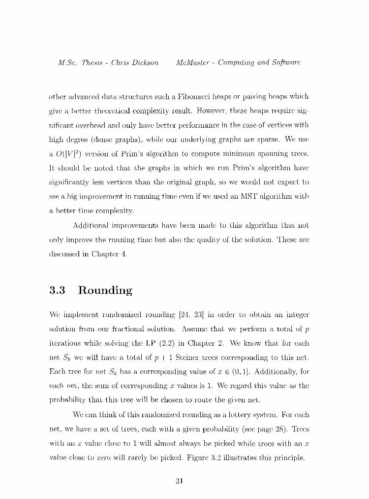
We can think of this randomized rounding as a lottery system. For each
net, we have a set of trees, each with a given probability (see page 28). Trees
with an x value close to 1 will almost always be picked while trees with an x
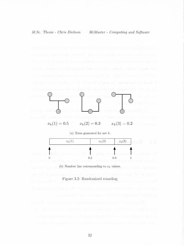
value close to zero will rarely be picked. Figure 3.2 illustrates this principle.
31
M.Sc. Thesis - Chr-is Dickson McMaster- Computing and Software
Xk (l) = 0.5 Xk(2) = 0.3 Xk(3) = 0.2
(a) Trees generated for net k .
x!.:( l ) I Xk(2) I Xk(3) I
t t t t 0 0.5 0.8 1
(b) Number line corresponding to Xk values .
Figure 3.2: Randomized rounding
32
M.Sc. Thesis - Chris Dickson McMaster- Computing and Software
In Figure 3.2(a) we have 3 trees generated for net k. Below each tree
we see the xk value associated with its respective tree. We map these values
to a number line over [0, 1) as shown in Figure 3.2(b). Each tree is associated
with a range of values over this number line. For each net k = 1, ... , K, we
generate a random number over [0, 1) to find the tree that will be chosen to
route net k. For example, if the random number was in the range [0, 0.5), the
first tree for net k would be chosen. If the random number was in the range
[0.5, 0.8), the second tree would be chosen. The tree corresponding to xk(T)
that is chosen to route net k is assigned the value 1, while other trees for net
k are assigned the value 0.
In practice, we repeat randomized rounding several times in order to
obtain the best possible solution. The amount of time spent in rounding is
extremely small compared to the time spent generating trees and solving the
LP. Also, in the case that we cannot generate a feasible integer solution, we
only keep solutions which have fewer constraint violations than the solutions
that came previously. In the case of ties in the number of edge capacity
violations, we keep the solution that has the lowest objective value.
33
M.Sc. Thesis - Chris Dickson McMaster- Computing and Software
34
Chapter 4
Heuristics and Improvements
We now show some practical improvements we have made to this algorithm.
We will present the details of choosing the step length T in this chapter. As
well, we will discuss some improvements made to the running time of the
Steiner tree solver. A multithreaded version of the algorithm is discussed, as
well as several heuristics used to improve the quality of the solution.
4.1 Potential Function Minimization
We base our LP solver on a g1ven algorithm for solving convex mm-max
resource-sharing problems. A potential function for convex min-max resource-
sharing problems (2.3) is introduced in [13] as follows:
t M
c/Jt(x) = lne- M L ln(e- f~n(x)), ( 4.1) m=l
where t is a parameter depending on the error tolerance E and the parameter
35
M.Sc. Thesis - Chris Dickson McMaster- Computing and Software
e is the solution of the following equation:
t M e M ~ e ~ frn(x) = 1.
(4.2)
It is shown in [13] that a good approximation of the minimum of ,\
can be attained at an x minimizing the potential function c/Yt ( x). The approx
imation algorithm for convex min-max resource-sharing problems in [13] is
based on this property and is applied in [26] for developing the approximation
algorithm for the VLSI global routing problem.
In this algorithm, there is a given formula to compute the step length
T. However, in practice we notice that this produces small values for T. This
causes the algorithm to converge slowly and thus requires many iterations
though the complexity bound in [26] still holds. Therefore, we need to decide
a relatively larger step length for speedup. On the other hand, we cannot
choose T to be too large. Otherwise our algorithm will begin to cycle and
converge slowly.
Our heuristic to determine the step length T is to find a new iterate x'
between the old iterate x and the block solution :i; by line search such that the
new fractional congestion f' minimizes the potential function c/Yt ( x) over all x'
between .T and .1:. We have used a bisection method in order to minimize this
function. Specifically, we approximate the derivative of the potential function
by using divided-differences as shown in equation ( 4.3) for some small 6 > 0.
(4.3)
We then find the zero of this function using the bisection method. It
should be noted that we have several fail-safe mechanisms for this line search.
We have safe-guarded a maximum number of iterations to avoid numerical
36
M.Sc. Thesis - Chris Dickson McMaster- Computing and Software
instability. Also, in the case that a zero does not exist, we simply use the
default step length. However, generally when no zero of the derivative to the
potential function can be found, the stopping criteria for solving the LP have
been met and the approximation bound has been reached. That is to say, no
step length can further reduce the congestion, so we can go no further.
4.2 Recording Shortest Paths
With regards to the Steiner tree solver, there are some simple improvements
that can be made to significantly reduce the running time. When we compute
Steiner trees, it is necessary to first compute a complete distance network of
the terminal set. This involves (1 5{1) calls to Dijkstra's algorithm for each net
Sk for k = 1 ... K. However, since in each iteration of our algorithm, we are
working with the same graph, the shortest paths from any given vertex in H
do not change. By storing the paths, we can eliminate the unnecessary calls to
Dijkstra's algorithm. Once we call Dijkstra's algorithm for a given terminal,
we can reduce the complexity of finding shortest paths to O(IVI) as we need
only to do a linear search to find the destination vertex, and trace its path back
to the source vertex. This technique yields a great improvement in running
time, especially for large instances with many nets. The only drawback is that
this significantly increases the memory demand on the system. After each
iteration, we must re-weight the graph H. Thus, the stored paths are only
valid for the current iteration and must be computed again in the following
iteration.
37
M.Sc. Thesis - Chris Dickson McMaster- Computing and Software
4.3 Parallel Tree Generation
Similar to the improvement we made in the Steiner tree solver, we are able to
exploit the fact that the graph weights remain constant throughout a given
iteration. Because of this, we may generate trees in any order without changing
the result of the solution. This naturally leads to the idea of parallelization. If
NP is the number of processes on our machine, then we may assign a total of
NP threads to generate trees. We can assume that, for each instance, each net
is labeled from 1 to K where K is the total number of nets. We assign each
thread a lower bound and an upper bound which represent the range of nets for
which it must produce trees. Specifically, each thread will generate lff J trees. p
We also assign the last thread the additional K mod NP trees. It is worth
noting that since K is generally much larger than NP, these additional trees
do not have a large effect on upsetting the workload balance for each thread.
In Chapter 5 we will provide computational results on the time improvement
using this technique.
4.4 Hybridization of Concurrent and Sequen-
tial Routing
The motivation for this heuristic is that sequential routers are generally able
to find a good solution in terms of feasibility, but not in terms of wire-length.
However, if we begin our algorithm with a "good" set of trees, then we may be
able to improve the total wire-length of the solution, while still maintaining
as much feasibility as possible.
In our implementation, we allow the solutions from a sequential router
38
M.Sc. Thesis - Chris Dickson McMaster- Computing and Software
called Labyrinth [18] to warm start our algorithm. Labyrinth uses the ma7oe
runner heuristic introduced by Lee in [19]. While being very good at finding
feasible solutions, Labyrinth has serveral limitations. First, the grid graph
must be uniform. That is, there may not be holes (missing vertices) in the
graph. Also, capacity must be uniform across the graph, restricted to a single
horizontal and vertical value. Additionally, this program does not take into
account vias or bends in the trees. We may use the solutions produced by
Labyrinth to reduce the running time of our own algorithm. However, m
order to fully exploit this technique, further investigation is needed.
4.5 Fixing Trees
Another class of heuristics that have been implemented deal with a fixing a
subset of nets to a single tree generated in the first iteration. The idea is to
determine a certain subset of the K total nets, and generate only a single tree
for this net. A similar heuristic has been implemented in [18] which allows
the user to route all 2-terminal nets first. A side effect of our heuristic is that
after the first iteration, we reduce the number of nets we need to find trees for
in subsequent iterations. This reduces the problem size, and thus reduces the
overall time taken to solve the problem.
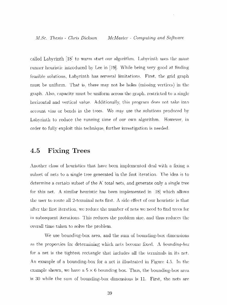
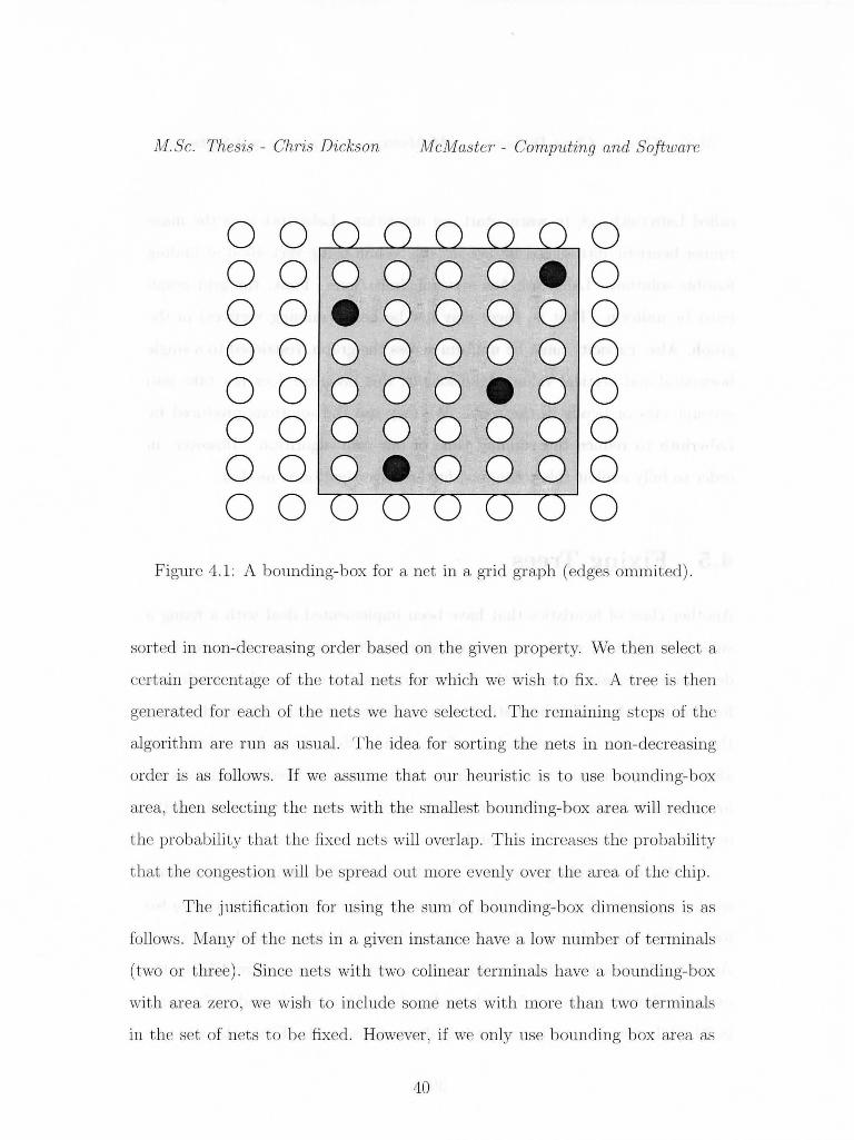
We use bounding-box area, and the sum of bounding-box dimensions
as the properties for determining which nets become fixed. A bounding-bo:r;
for a net is the tightest rectangle that includes all the terminals in its net.
An example of a bounding-box for a net is illustrated in Figure 4.5. In the
example shown, we have a 5 x 6 bounding box. Thus, the bounding-box area
is 30 while the sum of bounding-box dimensions is 11. First, the nets are
39
M.Sc. Thesis - Chris Dickson McMaster- Computing and Software
00 0 ooooooeo ooeooooo 00000000 oooooeoo 00000000 oooeoooo 00 0
Figure 4.1: A bounding-box for a net in a grid graph (edges ommited).
sorted in non-decreasing order based on the given property. We then select a
certain percentage of the total nets for which we wish to fix. A tree is then
generated for each of the nets we have sel cted . The remaining steps of the
algorithm are run as usual. The idea for sorting the nets in non-decreasing
order is as fo llows. If we assume that our heurist ic is to use bounding-box
area, then selecting the nets with the smallest bounding-box area will reduce
the probability that the fixed nets will overlap. This increases the probability
that the congestion will be spread out more evenly over the area of the chip.
The justification for using the sum of bounding-box dimensions is as
follows. Many of the nets in a given instance have a low number of terminals
(two or three). Since net s with two colinear terminals have a bounding-box
with area zero , we wish to include some nets with more than two terminals
in the set of nets to be fixed. However, if we only use bounding box area as
40

M.Sc. Thesis - Chris Dickson McMaster- Computing and Software
a heuristic to fix nets, we arc guaranteed to fix all colinear two terminal nets
first. By using the dimension sum heuristic, we add the possibility to fix nets
with a higher number of terminals. This is desirable as some two terminal nets
may be very long, while some three terminal nets may be very close together.
Another issue that arises in the discussion of this class of heuristics, is
how to appropriately choose the percentage of nets to fixed for a given instance.
In general, there is no way to determine ahead of time what percentage will
work the best for a given problem. Additionally, we have tried sorting in non
increasing order, but this method showed no improvement. In Chapter 5 we
will aim to determine some trends for a given set of benchmarks and show
that the use of any of these heuristics leads to some improvement.
41
M.Sc. Thesis - Chris Dickson McMaster- Computing and Software
42
Chapter 5
Computational Results
In this chapter we provide the computational results for our algorithm, as well
as for all the heuristics described in Chapter 4. We use the well-known MCNC
benchmark collection for our computational tests [20]. All codes are written
in C and all experiments are performed on an 8x AMD dual-core Opteron 885
workstation with 64GB of RAM running OpenSUSE 10.2 Linux. All running
times are reported in seconds.
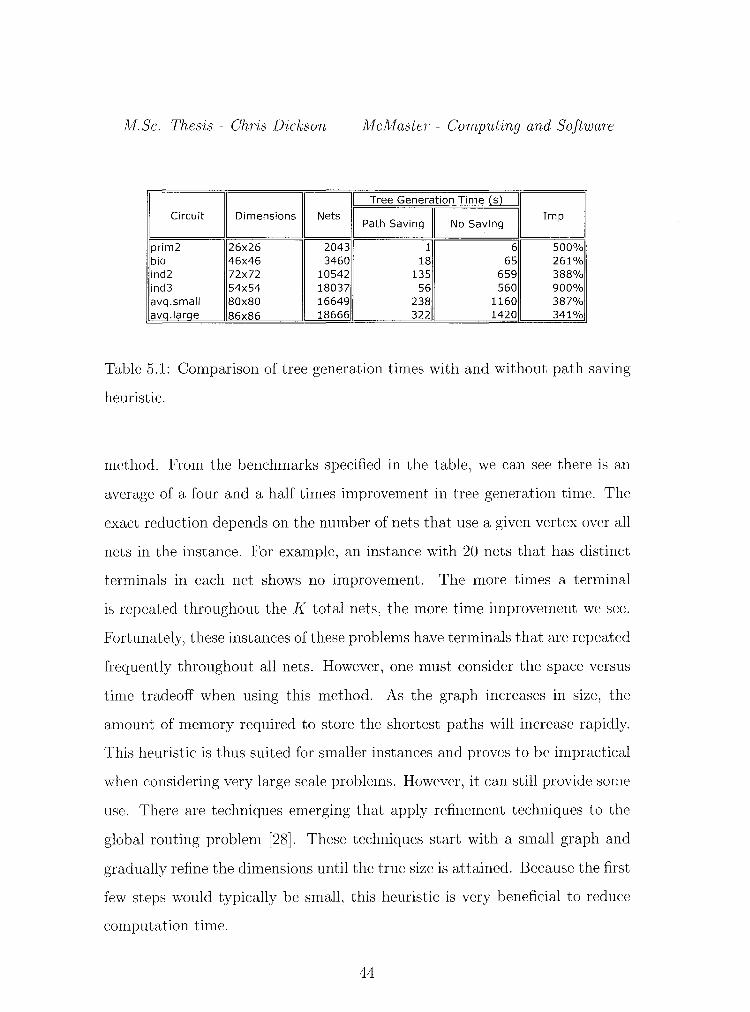
We begin with a comparison of the two mam versiOns of our code.
The first uses the path saving heuristic. The table in Table 5.1 compares the
running times of the algorithm without the heuristic versus using the heuristic.
Only the running time for solving the LP is given because time taken to round
the fractional solution is independent of the method used to solve the LP. It
should be noted that only the largest sets of test data are shown in this table
because the running times of small test sets are less than 1 second for both
versiOns.
As we can see, the time spent generating trees is greatly reduced using this
43
M.Sc. Thesis - Chris Dickson McMaster- Computing and Software
B E] Tree Generation Time {s) IG Dimensions Path Saving II I Imp No Saving
prim2 26x26 2043 1 6 500% bio 46x46 3460 18 65 261% ind2 72x72 10542 135 659 388% ind3 54x54 18037 56 560 900% avq.small 80x80 16649 238 1160 387% avq.large 86x86 18666 322 1420 341%
Table 5.1: Comparison of tree generation times with and without path saving
heuristic.
method. From the benchmarks specified in the table, we can see there is an
average of a four and a half times improvement in tree generation time. The
exact reduction depends on the number of nets that use a given vertex over all
nets in the instance. For example, an instance with 20 nets that has distinct
terminals in each net shows no improvement. The more times a terminal
is repeated throughout the K total nets, the more time improvement we see.
Fortunately, these instances of these problems have terminals that are repeated
frequently throughout all nets. However, one must consider the space versus
time tradeoff when using this method. As the graph increases in size, the
amount of memory required to store the shortest paths will increase rapidly.
This heuristic is thus suited for smaller instances and proves to be impractical
when considering very large scale problems. However, it can still provide some
usc. There are techniques emerging that apply refinement techniques to the
global routing problem [28]. These techniques start with a small graph and
gradually refine the dimensions until the true size is attained. Because the first
few steps would typically be small, this heuristic is very beneficial to reduce
computation time.
44
M.Sc. Thesis - Chris Dickson McMaster- Computing and Software
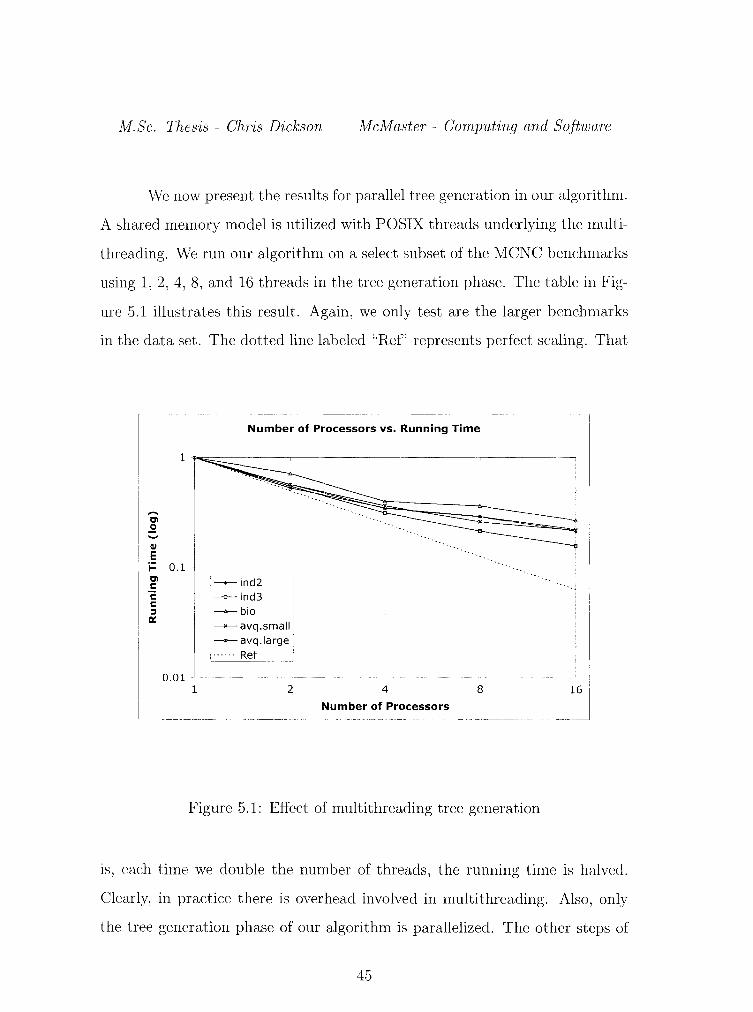
We now present the results for parallel tree generation in our algorithm.
A shared memory model is utilized with POSIX threads underlying the multi
threading. We run our algorithm on a select subset of the MCNC benchmarks
using 1, 2, 4, 8, and 16 threads in the tree generation phase. The table in Fig
ure 5.1 illustrates this result. Again, we only test are the larger benchmarks
in the data set. The dotted line labeled "Ref' represents perfect scaling. That
1
...... en .2 ....... Q)
E j:: 0.1 en r:: ·c: r:: :I a:
0.01 1
Number of Processors vs. Running Time
'-+- ind2 --o-ind3 ___,._ bio
--------- avq. sma II -•- avq.large
) ...... Ref
2 4 8
Number of Processors
Figure 5.1: Effect of multithreading tree generation
---l~J
1s, each time we double the number of threads, the running time is halved.
Clearly, in practice there is overhead involved in multithreading. Also, only
the tree generation phase of our algorithm is parallelized. The other steps of
45
M.Sc. Thesis - Chris Dickson McMaster- Computing and Software
the algorithm such as updating the edge weights in the graph, and computing
step lengths are not performed in parallel. However, we can still see that our
algorithm scales very well. This is due to the fact that the majority of the
running time in each iteration is spent in generating trees. Thus, speeding up
tree generation has a large effect on speeding up the whole algorithm.
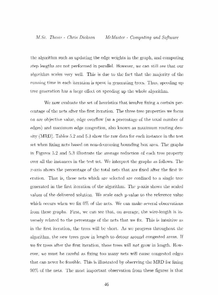
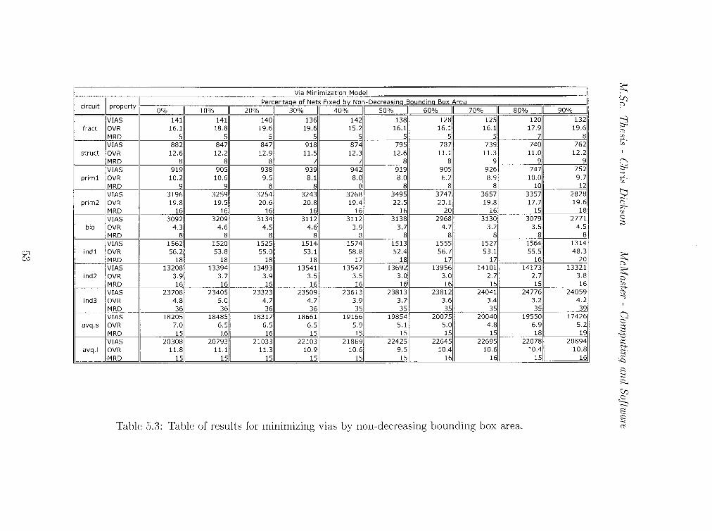
We now evaluate the set of heuristics that involve fixing a certain per
centage of the nets after the first iteration. The three tree properties we focus
on are objective value, edge overflow (as a percentage of the total number of
edges) and maximum edge congestion, also known as maximum routing den
sity (MRD). Tables 5.2 and 5.3 show the raw data for each instance in the test
set when fixing nets based on non-decreasing bounding box area. The graphs
in Figures 5.2 and 5.3 illustrate the average reduction of each tree property
over all the instances in the test set. We interpret the graphs as follows. The
x-axis shows the percentage of the total nets that are fixed after the first it
eration. That is, these nets which are selected are confined to a single tree
generated in the first iteration of the algorithm. The y-axis shows the scaled
values of the delivered solution. We scale each y-value to the reference value
which occurs when we fix 0% of the nets. We can make several observations
from these graphs. First, we can see that, on average, the wire-length is in
versely related to the percentage of the nets that we fix. This is intuitive as
in the first iteration, the trees will be short. As we progress throughout the
algorithm, the new trees grow in length to detour around congested areas. If
we fix trees after the first iteration, these trees will not grow in length. How
ever, we must be careful as fixing too many nets will cause congested edges
that can never be feasible. This is illustrated by observing the MRD for fixing
90% of the nets. The most important observation from these figures is that
46
M.Sc. Thesis - Chris Dickson McMaster- Comp1Lting and Software
fixing nets significantly reduces the number of infeasible edges. On average,
we see that fixing 70% of the nets based on non-decreasing bounding box area
gives the global minimum for overflow. We also see that MRD is decreased at
this percentage, and in the case of wire-length minimization, the minimum for
overflow and MRD occur at the same fixing percentage.
120%
115%
110%
g 105% :i:i ~ 100% 'C Ql
0::: 95% -Ql
~ 90% .. ,_ Ql
~ 85%
80%
Bounding-Box Area (WL Minimization)
.... ,- . .
! ---- Wirelength '---Overflow
····· MRD
75% +------------------------------------------
0 10 20 30 40 50 60 70 80 90
Percentage Fixed
Figure 5.2: Average reduction for minimizing wire-length by non-decreasing
bounding box area.
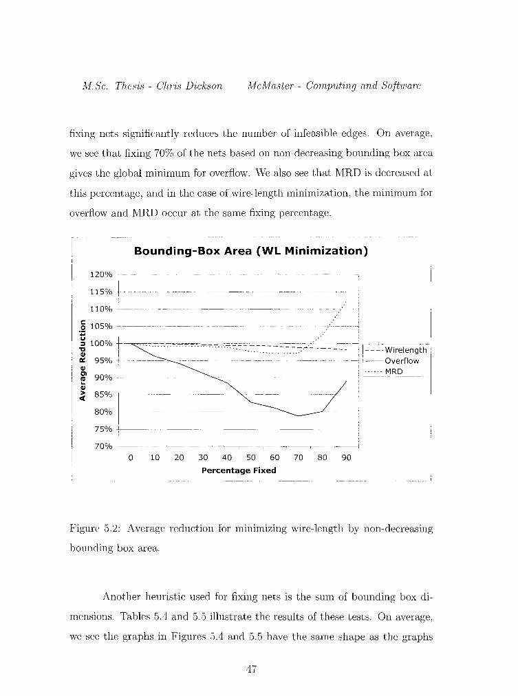
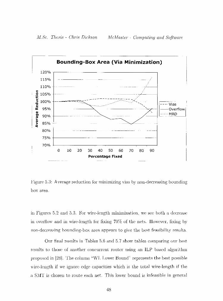
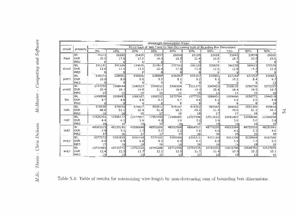
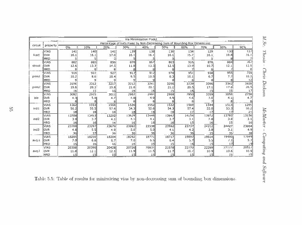
Another heuristic used for fixing nets is the sum of bounding box di
mensions. Tables 5.4 and 5.5 illustrate the results of these tests. On average,
we see the graphs in Figures 5.4 and 5.5 have the same shape as the graphs
47
M.Sc. Thesis - Chris Dickson McMaster- Computing and Software
Bounding-Box Area (Via Minimization)
120o/o ·,----------------------------------------,
115%
110% 1: 0 105% -
',j::i u
~------- ~------~ ---
.· --.------
:I 100% - - __ ....,....,=;;:;;;:;;. _:;.,_ ~ 'C
------ ~-~ ~-~--~-"-<c-co-~~1.:.: ..... ;;;;,:-
CIJ ,,
' cr:: 95%-1--- ' --------....----CIJ Cl 90% ------rg .. CIJ
85% > <(
80% - --- -----------
75%
70%
0 10 20 30 40 50 60 70 80 90
Percentage Fixed
Figure 5.3: Average reduction for minimizing vias by non-decreasing bounding
box area.
in Figures 5.2 and 5.3. For wire-length minimization, we see both a decrease
in overflow and in wire-length for fixing 70% of the nets. However, fixing by
non-decreasing bounding-box area appears to give the best feasibility results.
Our final results in Tables 5.6 and 5. 7 show tables comparing our best
results to those of another concurrent router using an ILP based algorithm
proposed in [28]. The column "WL Lower Bound" represents the best possible
wire-length if we ignore edge capacities which is the total wire-length if the
a SMT is chosen to route each net. This lower bound is infeasible in general
48
M.Sc. Thesis - Chris Dickson McMaster- Computing and Software
I C
120%-
115%
110%
.!2 105% -... u .g 100% Ql a:: 95% Ql
g' 90% L. Ql >
<C 85%-
80%
Bounding-Box Sum of Dimensions (WL Minimization)
-----l
-------- l 75%-1---
70% 0 10 20 30 40 so 60 70 80 90
Percentage Fixed --- ___ I
Figure 5.4: Average reduction for minimizing wire-length by non-decreasing
sum of bounding box dimensions.
because the capacity constraints are violated on many edges. GeoSteiner v3.1
is used to find optimal SMT's [9]. In [28], they make the assumption that
any net with 10 or more terminals may be ignored by the global router. For
fairness, we also make this assumption. They perform tests on a 900 MHz Sun
Blade 200 workstation with 1GB of memory. Additionally, they use CPLEX
8.0 as a solver for their ILP. On the other hand, our implementation use no
commercial software.
For wire-length minimization, we find that our algorithm finds a more
49
M.Sc. Thesis - Chris Dickson McMaster- Computing and Software
120%
115%
110% c .!2 105% .... u ~ 100% (II ~ 95% (II
~~----- ~ ~~-----~- -~ ------- ~---
Bounding-Box Sum of Dimensions (Via Minimization)
+---------------="<--------~+----- ~-------: ~i::rflow Cl 90%-Ill
l::··_-: MRD .. (II
85% > c(
80%
75%
70%
0 10 20 30 40 50 60 70 80 90
Percentage Fixed
Figure 5.5: Average reduction for minimizing vias by non-decreasing sum of
bounding box dimensions.
feasible solution than in [28] in almost all test cases. As well, it can be seen
that wire-length is not greatly sacrificed in order to achieve a reduction in
the maximum routing demand. On average, we reduce the maximum routing
demand by 25.8% while only increasing the wire-length by 1.4%. It is crucial
that our algorithm is able to get a solution with fewer capacity violations, as
feasibility is the most important and challenging issue in the global routing
problem.
We see a similar situation for our via minimization model. Although
50
M.Sc. Thesis - Chris Dickson McMaster- Computing and Software
we have a larger number of vias in our solutions, in almost all cases we im
prove the maximum routing demand significantly. In the best case, we see a
36% improvement in MRD, while on average, an improvement of 30% is seen.
Again, it should be noted that feasibility is always the most important issue.
Furthermore, we see that our via minimization model reduces the number of
vias by an average of 4% over our wire-length minimization model.
In terms of running time, it can be seen that our algorithm is of the
same order as the algorithm presented in [28]. It should be noted that in Table
1 of [28] they present an edge congestion minimization model. Comparing
these results with ours in Tables 5.6 and 5.7, we find that our MRD is very
close to the MRD presented in [28]. Additionally, in order for them to achieve
this improvement in edge congestion, they require a significant amount of
additional computation time. On the largest problems, they see a 55% increase
in running time on average, and 68% for the largest instance.
51
\IF=====~====~============================~W~ir~el~e~ng~t~h~M~i~n~tm~i~za~t~io~n~M~o~d~e~l==~==~====7=============================~ II circuit llproperty 1!~1\ ==~====¥===~==~r=~~==~P~er~c~en~t~a~ge~F~ix~ed~b~y~N~o~n~-D~e~c~re~a~s~in~g~B~o~u~n~di~n~g~B~o~x~A~re~a~~~===v==~~==~==~~~ o% 1o% 20% II 30% II 40% II so% II 60% II 70% 80% 90%
WL 26323 26310 26078 25970 26106 26568 26255 25834 25942 25942 fract OVR 20.5 18.8 17.9 18.7 19.6 15.2 17.8 16.0 14.2 17.0
MRD 6 6 6 6 6 6 6 6 7 7 WL 341141 342055 339882 339098 330350 329441 330237 321812 321698 322264
struct OVR 13.6 13.8 13.2 12.7 11.0 11.7 10.7 10.7 11.4 11.0 MRD 8 8 8 8 8 8 7 9 9 9 WL 638371 637382 638371 637792 636913 637502 636334 646442 638327 636859
prim1 OVR 10.0 9.0 9.9 10.2 8.4 8.3 7.9 9.3 8.0 9.0 MRD 9 9 9 9 9 9 9 8 11 13 WL 3343050 3342560 3311273 3306075 3309998 3318727 3306271 3298621 3328240 3264687
prim2 OVR 20.4 20.0 19.8 18.6 19.9 19.2 19.0 18.0 17.4 19.2 MRD 15 15 15 15 15 15 15 15 14 16 WL 1066898 1072331 1082989 1084025 1086162 1079402 1075817 1070599 1063371 1046830
bio OVR 4.7 4.7 3.7 4.4 3.8 3.5 3.2 3.2 3.6 4.1 MRD 8 8 8 8 8 8 8 8 7 9 WL 978558 977522 977376 972687 976361 980229 987628 986800 981950 994924
ind1 OVR 48.8 51.1 49.5 49.0 50.2 50.0 51.1 51.4 50.4 53.3 MRD 18 18 18 18 18 17 17 17 17 19 WL 12625392 12570171 12570749 12550187 12499592 12483828 12419794 12414983 12390044 12322415
ind2 OVR 4.4 3.9 3.8 3.5 3.4 2.7 2.8 2.5 2.5 3.9 MRD 16 16 16 16 16 15 16 15 15 17 WL 49083925 49063802 49161481 48970406 48877719 48815338 48795539 48590970 48358063 48053830
ind3 OVR 4.9 4.9 4.9 4.0 4.2 4.2 3.8 3.2 3.3 4.4 MRD 37 36 36 36 35 35 35 35 36 39 WL 9377272 9368794 9342804 9338653 9317210 9252418 9260603 9260833 9199266 9179896
avq.s OVR 6.6 6.4 6.8 6.4 6.3 5.3 5.1 4.8 6.3 5.2 MRD 17 16 16 16 16 16 16 15 17 18 WL 10724983 10753773 10718299 10701025 10687063 10658180 10590604 10566493 10566020 10537304
avq.l OVR 12.4 11.3 11.4 10.3 10.5 10.8 10.3 10.1 10.4 10.9 MRD 15 15 15 15 15 15 15 15 16 16
Table 5.2: Table of results for minimizing wire-length by non-decreasing bounding box area.
CJl w
IF=====~====~r================================V~iga~M~in~i~m~iz~a~ti~ogn~M~o~d~e~l============================================~
II circuit llpropertylll~~~===v==~~==~==~~P~e~rc~e~n~ta~q~e~o~f~N~e~tshFgi~xe~d~by~Ngo~n-~D~e~c~re~a~si~nga~B~ogu~nd~i~nq~Bgox~Agre~a~~==~==~~==w=~~~~
o% 1o% 2o% II 30% II 40% II so% II 60% II 70% 80% 90% VIAS 141 141 140 136 142 138 128 125 120 132
fract OVR 16.1 18.8 19.6 19.6 15.2 16.1 16.1 16.1 17.9 19.6 MRD 5 5 5 s 5 5 5 5 7 8 VIAS 882 847 847 918 874 795 787 739 740 762
struct OVR 12.6 12.2 12.9 11.5 12.3 12.6 11.1 11.3 11.0 12.2 MRD 8 8 8 7 7 8 8 9 9 9 VIAS 919 905 938 939 942 919 905 926 747 752
prim1 OVR 10.2 10.6 9.5 8.1 8.0 8.0 6.2 8.9 10.0 9.7 MRD 9 9 8 8 8 8 8 8 10 12 VIAS 3196 3259 3254 3243 3268 3495 3747 3657 3357 2828
prim2 OVR 19.8 19.5 20.6 20.8 19.4 22.5 23.1 19.8 17.7 19.6 MRD 16 16 16 16 16 16 20 16 15 18 VIAS 3092 3209 3134 3112 3112 3138 2968 3130 3079 2771
bio OVR 4.3 4.6 4.5 4.6 3.9 3.7 4.7 3.2 3.5 4.5 MRD 8 8 8 8 8 8 8 8 8 8 VIAS 1562 1520 1525 1514 1574 1513 1555 1527 1564 1314
ind1 OVR 56.2 53.8 55.0 53.1 58.8 52.4 56.7 53.1 55.5 48.3 MRD 18 18 18 18 17 18 17 17 16 20 VIAS 13208 13394 13493 13541 13547 13692 13956 14101 14173 13321
ind2 OVR 3.9 3.7 3.9 3.5 3.5 3.0 3.0 2.7 2.7 3.8 MRD 16 16 16 16 16 16 16 15 15 16 VIAS 23708 23405 23323 23509 23613 23813 23812 24041 24776 24059
ind3 OVR 4.8 5.0 4.7 4.7 3.9 3.7 3.6 3.4 3.2 4.2 MRD 36 36 36 36 35 35 35 35 35 39 VIAS 18205 18485 18317 18661 19166 19854 20075 20040 19550 17426
avq.s OVR 7.0 6.5 6.5 6.5 5.9 5.1 5.0 4.8 6.9 5.2 MRD 15 16 16 15 15 15 15 15 18 19 VIAS 20308 20793 21033 22103 21869 22425 22645 22695 22078 20894
avq.l OVR 11.8 11.1 11.3 10.9 10.6 9.5 10.4 10.6 10.4 10.8 MRD 15 15 15 15 15 15 16 16 15 16
Table 5.3: Table of results for minimizing vias by non-decreasing bounding box area.
Wirelength Minimization Model
I circuit II property II Percentage of Nets Fixed by Non-Decreasing Sum of Bounding Box Dimensions I!
0% II 10% II 20% I 30% 40% I 50% II 60% II 70% II 80% II 90% II WL 26323 26282 26459 25657 26064 26105 25928 25942 25874 26010
fract OVR 20.5 17.8 17.8 16.0 16.9 21.4 16.9 18.7 20.5 19.6 MRD 6 6 6 6 7 6 7 6 7 8 WL 341141 341596 339659 337847 337393 340120 339659 340230 348423 325526
struct OVR 13.6 11.5 13.5 12.6 12.9 13.0 12.5 12.0 14.2 12.6 MRD 8 8 8 8 8 8 8 8 7 8 WL 638371 638081 638606 638084 636093 635157 635803 637264 637202 636682
prim1 OVR 10.0 8.0 9.6 9.5 8.1 9.2 8.1 10.2 8.4 9.7 MRD 9 9 9 9 9 9 9 9 9 13 WL 3343050 3348444 3349523 3345012 3340304 3311175 3349425 3308135 3296758 3272337
prim2 OVR 20.4 18.7 19.8 21.4 18.8 19.3 20.4 18.4 18.5 18.7 MRD 15 15 15 15 15 15 15 15 15 16 WL 1066898 1068483 1066167 1068312 1073764 1077721 1086837 1089886 1056772 1044278
bio OVR 4.7 4.8 4.9 4.4 4.7 4.4 4.2 3.6 3.9 4.8 MRD 8 8 8 8 8 8 8 8 8 10 WL 978558 978035 979427 983811 978167 974302 985342 984002 1001389 959610
ind1 OVR 48.8 51.1 50.4 51.6 50.2 49.2 51.4 49.0 51.1 44.7 MRD 18 18 18 17 18 18 17 17 18 29 WL 12625392 12596127 12577901 12561699 12546085 12525594 12511655 12461403 12404046 12364204
ind2 OVR 4.4 4.1 3.9 4.0 3.9 3.2 3.4 3.0 3.0 3.6 MRD 16 16 16 16 16 16 16 16 16 16 WL 49083925 49155196 49186648 48952696 48950568 48864517 48779295 49033084 48755553 48251991
ind3 OVR 4.9 5.0 5.7 5.0 5.2 4.6 4.6 4.1 3.5 4.6 MRD 37 36 37 37 37 36 36 35 35 38 WL 9377272 9392839 9391456 9374161 9399066 9355371 9331160 9301299 9228664 9182548
avq.s OVR 6.6 6.9 6.8 6.3 6.5 6.2 6.0 5.5 7.3 5.5 MRD 17 16 16 16 16 16 16 15 18 18 WL 10724983 10735772 10752310 10745288 10712496 10751935 10762003 10645796 10645781 10537878
avq.l OVR 12.4 12.0 11.7 12.1 12.0 11.7 11.4 10.5 10.2 10.1 MRD 15 15 15 15 15 15 15 15 15 16
Table 5.4: Table of results for minimizing wire-length by non-decreasing sum of bounding box dimensions.
Via Minimization Model I
I circuit II property II Percentage of Nets Fixed by Non-Decreasing Sum of Bounding Box Dimensions
II 0% II 10% II 20% II 30% II 40% II 50% II 60% II 70% II 80% II 90% I VIAS 141 140 141 139 138 136 134 129 130 127
fract OVR 16.1 16.1 17.0 16.1 16.1 16.1 15.2 16.1 18.8 16.1 MRD 5 5 5 5 5 5 5 5 8 7 VIAS 882 885 856 876 867 863 916 878 884 767
struct OVR 12.6 13.3 14.5 11.8 13.3 12.5 13.9 10.7 12.1 12.5 MRD 8 8 8 8 8 8 7 8 7 8 VIAS 919 922 927 913 912 978 951 938 955 759
prim1 OVR 10.2 8.6 10.4 9.5 10.5 8.3 10.1 6.7 7.2 10.2 MRD 9 9 9 9 9 8 8 8 8 12 VIAS 3196 3312 3217 3212 3241 3296 3239 3396 3342 2858
prim2 OVR 19.8 20.5 19.8 21.6 20.1 21.1 20.5 17.1 17.8 20.5 MRD 16 15 16 16 16 15 16 15 15 17 VIAS 3092 2915 3011 2962 2984 2968 2950 3359 3050 2758
bio OVR 4.3 5.0 4.2 4.8 4.9 4.9 4.6 3.0 4.1 4.7 MRD 8 8 8 8 8 8 8 7 8 8 VIAS 1562 1553 1558 1526 1552 1532 1569 1544 1513 1295
ind1 OVR 56.2 55.5 57.6 54.3 52.6 54.3 57.4 55.0 53.3 50.2 MRD 18 18 18 18 18 18 17 17 17 21 VIAS 13208 13453 13292 13629 13446 13842 14154 13972 13793 13156
ind2 OVR 3.9 3.7 4.1 4.1 4.1 3.7 3.1 2.8 3.0 3.1 MRD 16 16 16 16 16 16 15 16 15 16 VIAS 23708 23297 23679 23692 23538 23592 23737 24212 24427 23864
ind3 OVR 4.8 5.5 4.9 5.0 5.0 4.1 4.2 3.8 3.1 4.9 MRD 36 37 36 36 36 36 36 35 35 38 VIAS 18205 18256 18204 18292 18771 18717 19097 19614 19490 17049
avq.s OVR 7.0 6.8 6.7 7.0 6.5 6.4 5.7 5.5 7.1 5.7 MRD 15 16 16 16 15 15 16 15 17 19 VIAS 20308 20390 20428 20726 20831 21078 22270 22289 22177 20517
avq.l OVR 11.8 12.1 12.1 11.9 11.5 11.7 10.7 10.9 10.6 10.9 MRD 15 15 15 15 15 15 15 15 15 15
Table 5.5: Table of results for minimizing vias by non-decreasing sum of bounding box dimensions.
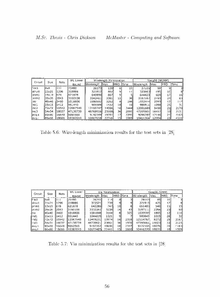
M.Sc. Thesis - Chris Dickson McMaster- Computing and Software
Circuit Size
fract 8x8 struct 21x21 1296 318886 prim1 19x19 678 621878 644423 prim2 26x26 2043 3160108 3 3187597 bio 46x46 3460 1018806 186 1032444 ind1 15x15 1412 951440 10 986911 ind2 72x72 10542 12067540 12091689 9490 ind3 54x54 18037 47130739 47205901 16457 avq.s 80x80 16649 9065565 9192349 9096280 12146 av .I 86x86 18666 10382010 10667658 10411364 12994
Table 5.6: Wire-length minimization results for the test sets in [28]
I Circuit IBB WL Lower Bound
fract 8x8 111 25480 struct 21x21 1296 318886 prim1 19x19 678 621878 prim2 26x26 2043 3160108 43 3197111 bio 46x46 3460 1018806 1081848 325 1039595 ind1 15x15 1412 951440 1044835 9 7 989845 ind2 72x72 10542 12067540 12499231 16 2318 12114767 ind3 54x54 18037 47130739 48730621 36 1970 47395661 avq.s 80x80 16649 9065565 919235 2347 9122104 av .I 86x86 18666 10382010 1067248 5660 10446320
Table 5. 7: Via minimization results for the test sets in [28]
56
Chapter 6
Conclusions and Future Work
In this thesis, we have presented a polynomial time approximation algorithm
for the global routing problem in VLSI design which has a theoretical approx
imation bound. We provide a serial as well as a parallel implementation of
this approximation algorithm. In practice, our solutions are much closer to
optimality than the bound suggests. From Table 5.6 we find there is very little
gap between the lower bounds for the optimal solutions and our approximate
solutions. On average, we find that we are within 3% of the lower bound on
wire-length, and in some cases, less than 1% while the theoretical approxima
tion ratio is 2.
A number of techniques and heuristics have been developed to improve
the objective function value, as well as reduce computation time.
We have found that by preserving the shortest paths computed through
out an iteration of our algorithm, we can reduce the running time of our serially
implemented algorithm by nearly a factor of 5 on average and up to a factor of
9. Additionally, we have presented a parallel implementation of the algorithm
which allows for a significant reduction in running time, as well as lower mem-
57
M.Sc. Thesis - Chris Dickson McMaster- Computing and Software
ory usage compared to our serial version which uses path saving. The tree
generation phase is multi-threaded in order to minimize the time spent in this
step of the algorithm. Since this is the most costly part of the algorithm in
terms of CPU time, we see that as the number of processors increases, our al
gorithm scales well, especially in the largest instances that contain many nets.
Our computational experiments also show that confining a certain percentage
of the total nets to a single tree not only lead to better feasibility results,
but help to improve the objective function value. On average, we find that
fixing 70% of the nets based on non-decreasing bounding box area reduces
the number of infeasible edges by nearly 22% while simultaneously reducing
the wire-length by nearly 2%. When minimizing vias, this heuristic is able to
reduce overflow by nearly 16%, while only leading less than a 2% increasing in
the number of vias. In the best case, this heuristic was able to reduce overflow
by more than 43% and wire-length by nearly 6%. Fixing by non-decreasing
bounding box sum of dimensions also proves to be a valuable heuristic to
this algorithm. On average, we also find that fixing 70% of the nets gives
the optimal reduction in overflow. Across the entire benchmark set, fixing
70% yields an 11% reduction in infeasible edges, while reducing wire-length
by close to 6%. When minimizing vias, this heuristic gives a 17% reducing
in infeasible edges, while sacrificing 3.2% in the number of vias. Additionally,
we have showed that our algorithm is very competitive with other ILP based
approaches and, in many cases, provides significantly better feasibility results
with similar objective values.
Our future work involves changing the way the edge congestion is esti
mated. We believe that by updating the edge congestion several times through
out a given iteration, we can improve the quality of the solution as well as
58
M.Sc. Thesis - Chris Dickson McMaster- Computing and Software
reduce the number of iterations required to obtain it. We plan to develop
new, fast techniques for tree generation which constitutes 98% of the total
time required for the algorithm. Such techniques may include Voronoi region
based partitioning/ compacting of the underlying graph [21].
59

M.Sc. Thesis - Chris Dickson McMaster- Computing and Software
60
Bibliography
[1] A.V. Aho, J.E. Hopcroft, and J.D. Ullman, Data Structur-es and Algo
r-ithms, Addison-Wesley, 1983.
[2] K.M. Anstreicher, Towar-ds a pr-actical volumetr-ic cutting plane method
for- convex pmgmmming, SIAM Journal on Optimization 9 (1999), 190-
206.
[3] G. Ausiello, P. Crescenzi, G. Gambosi, V. Kann, A. Marchetti
Spaccamela, and M. Protasi, Complexity and Appmximation: Combi
nator-ial Optimization Pmblems and Their- Appr-oximability Pmper-ties,
Springer-Verlag, 1999.
[4] J.A. Bondy and U.S.R. Murty, Gmph Theor-y and Applications, MacMil
lan, 1978.
[5] C.C.N. Chu, FLUTE: Fast lookup table based wir-elength estimation tech
nique, Proc. Internation Conference on Computer Aided Design, 2004,
pp. 696-701.
[6] T.H. Cormen, C.E. Leiserson, R.L. Rivest, and C. Stein, Intr-oduction to
Algor-ithms, seconded., The MIT Press, 2001.
61
M.Sc. Thesis - Chris Dickson McMaster- Computing and Software
[7] E.W. Dijkstra, A note on two problems in connexion with graphs, Nu
merische Mathematik 1 (1959), 269-271.
[8] M.R. Garey and D.S. Johnson, The Tectilinear Steiner problem is NP
complete, SIAM J. Appl. Math 32 (1977), 826-834.
[9] GeoSteiner Homepage: http:/ /www.diku.dk/geosteiner/. Retreived
March 18, 2007.
[10] M.D. Grigoriadis and L.G. Khachiyan, CooTdination complexity of paml
lel price-diTective decomposition, Mathematics of Operations Research 2
(1996), 321-340.
[11] M. Grotschel, L. Lovasz, and A. Schrijver, The ellipsoid method and
its consequences in combinatorial optimization, Combinatorica 1 ( 1981),
169-197.
[12] K. Jansen and H. Zhang, An approximation algorithm for the multicast
congestion problem via minimum Steiner trees, Proceedings of the 3rd
International Workshop on Approximation and Randomized Algorithms
in Communication Networks, 2002, pp. 77-90.
[13] , Approximation algorithms for geneml packing problems with mod-
ified logarithmic potential function, Proceedings of the 3rd International
Workshop on Approximation and Randomized Algorithms in Communi
cation Networks, 2002, pp. 255-266.
[14] M. Chlebfk and J. Chlebfkova, Approximation hardness of the Steiner tree
problem, Proceedings of the 8th Scandinavian Workshop on Algorithm
Theory, 2002, pp. 170-179.
62
M.Sc. Thesis - Chris Dickson McMaster- Computing and Software
[15] S.M. Kang andY. Leblebici, CMOS Digital Integrated Circuits, McGraw
Hill Publishing Company, Inc, 2003.
[16] L. Kou, G. Markowsky, and L. Berman, A fast algorithm for Steiner trees,
Acta Informatica 15 (1981), 141-145.
[17] J.B. Kruskal, On the shortest spanning subtree of a graph and the traveling
salesman problem, Proceedings of the American Mathematical Society 7
(1956), 48-50.
[18] Labyrinth: A global router and routing development tool.
http:/ /www.ece.ucsb.edu;-kastner/labyrinthj. Retrieved March 18,
2007.
[19] C.Y. Lee, An algoTithm joT path connection and its appl'ication, IRE
Transactions on Electronic Computers 10 (1961), 346-365.
[20] MCNC: http:/ jwww.cbl.ncsu.edu/benchmarks/layoutsynth92/. Re-
tTieved MaTch 26, 2007.
[21] K. Mehlhorn, A fasteT approximation algorithm for the Steiner problem
in graphs, Information Processing Letters 27 (1988), 125-128.
[22] R.C. Prim, ShoTtest connection netwoTks and some generalizations, Bell
System Technical Journal 36 (1957), 1389-1401.
[23] P. Raghavan, Probabilistic construction of deterministic algorithms: ap
pmximating packing integeT programs, Journal of Computer an System
Sciences 37 (1988), 130-143.
63
M.Sc. Thesis - Chris Dickson McMaster- Computing and Software
[24] P. Raghavan and C. D. Thompson, Randomized rounding: a technique for
provably good algorithms and algorithmic proofs, Combinatorica 7 (1987),
365-374.
[25] G. Robins and A. Zelikovsky, Improved Steiner tree approximation in
graphs, Proceedings of the 11th Anual ACM-SIAM Symposium on Dis
crete Algorithms, 2000, pp. 770-·779.
[26] T. Terlaky, A. Vannelli, and H. Zhang, On routing in VLSI design and
communication networks, Proceedings of the16th International Sympo
sium on Algorithms and Computation, 2005, pp. 1051-1060.
[27] D.M. Warme, Spanning trees in hypergraphs with applications to Steiner
trees, Ph.D. thesis, Computer Science Dept., The University of Virginia,
1998.
[28] Z. Yang, A. Vannelli, and S. Areibi, An ILP based hierarchical global
routing approach for VLSI ASIC design, Optimization Letters 1 (2007),
281-297.
., 4 2 9 1 1 64