global systems, local impacts: a spatially-explicit...

Environmental Change

Department of Thematic Studies

Linköping University

Master’s programme

Science for Sustainable Development

Master’s Thesis, 30 ECTS credits

Supervisor: Tina-Simone Schmid Neset

2015

Global Systems, Local Impacts: A Spatially-Explicit Water Footprint and

Virtual Trade Assessment of Brazilian Soy

Production

Rafaela Ariana Flach

Upphovsrätt

Detta dokument hålls tillgängligt på Internet – eller dess framtida ersättare – under 25 år från

publiceringsdatum under förutsättning att inga extraordinära omständigheter uppstår.

Tillgång till dokumentet innebär tillstånd för var och en att läsa, ladda ner, skriva ut

enstaka kopior för enskilt bruk och att använda det oförändrat för ickekommersiell forskning

och för undervisning. Överföring av upphovsrätten vid en senare tidpunkt kan inte upphäva

detta tillstånd. All annan användning av dokumentet kräver upphovsmannens medgivande.

För att garantera äktheten, säkerheten och tillgängligheten finns lösningar av teknisk och

administrativ art.

Upphovsmannens ideella rätt innefattar rätt att bli nämnd som upphovsman i den

omfattning som god sed kräver vid användning av dokumentet på ovan beskrivna sätt samt

skydd mot att dokumentet ändras eller presenteras i sådan form eller i sådant sammanhang

som är kränkande för upphovsmannens litterära eller konstnärliga anseende eller egenart.

För ytterligare information om Linköping University Electronic Press se förlagets hemsida

http://www.ep.liu.se/.

Copyright

The publishers will keep this document online on the Internet – or its possible replacement –

for a period of 25 years starting from the date of publication barring exceptional

circumstances.

The online availability of the document implies permanent permission for anyone to read,

to download, or to print out single copies for his/her own use and to use it unchanged for non-

commercial research and educational purpose. Subsequent transfers of copyright cannot

revoke this permission. All other uses of the document are conditional upon the consent of the

copyright owner. The publisher has taken technical and administrative measures to assure

authenticity, security and accessibility.

According to intellectual property law the author has the right to be mentioned when

his/her work is accessed as described above and to be protected against infringement.

For additional information about Linköping University Electronic Press and its procedures

for publication and for assurance of document integrity, please refer to its www home page:

http://www.ep.liu.se/.

© Rafaela Ariana Flach

SUMMARY

1 Abstract ........................................................................................................................... 1

2 Introduction .................................................................................................................... 2

2.1 Problem Formulation and Research Questions ........................................................ 3

3 Background and State of the Art .................................................................................... 4

3.1 Global Water System and Water Teleconnections .................................................. 4

3.2 Virtual Water and Water Footprint .......................................................................... 5

3.3 Water Footprint Framework: Opportunities and Limitations .................................. 7

3.4 Blue and Green Water Scarcity ............................................................................... 8

3.5 Trade Flow Accounting for Water Footprints ....................................................... 10

3.6 Commodity Trade and Water Resources in Brazil ................................................ 11

4 Materials and Methods ................................................................................................. 13

4.1 Crop Water Requirement Assessment Model ........................................................ 13

4.1.1 Climate Sensitivity ......................................................................................... 15

4.1.2 Production, Harvested Area and Yield Correction ......................................... 17

4.2 Water Stress and Scarcity Indicators in Brazil ...................................................... 20

4.2.1 Available Data ................................................................................................ 20

4.2.2 Water Stress, Scarcity and Irrigation Indicators ............................................. 21

4.2.3 Water Stress Typologies ................................................................................. 22

4.3 Spatially-Explicit Information on Production to Consumption Systems ............... 23

4.4 Data and Methodological Uncertainties................................................................. 23

5 Results .......................................................................................................................... 24

5.1 Water Footprint Accounting: Current Approach ................................................... 25

5.2 Water Footprints: Adapted Accounting ................................................................. 28

5.3 Water Footprints: Global Allocation ..................................................................... 29

5.4 Footprints and Water Stress Typology .................................................................. 34

5.4.1 Classification of Regions by Typology of Water Stress................................. 34

5.4.2 Water Footprints Classified by Stress Typologies ......................................... 38

5.5 Brazilian Soy: Swedish Water Footprints .............................................................. 44

6 Discussion and Concluding Remarks ........................................................................... 48

2

6.1 Proposed Approach to Water Footprint Accounting: Improvements and Added

Knowledge ........................................................................................................................ 48

6.2 Assessment of Blue and Green Water Sustainability ............................................ 49

6.3 Global Trade, Local Impacts.................................................................................. 50

6.4 Recommendations for Future Research ................................................................. 51

7 Acknowledgements ...................................................................................................... 53

8 References .................................................................................................................... 54

LIST OF FIGURES

Figure 1 Methods and approaches for virtual water and water footprint accounting (Adapted

from Yang et al., 2013, p. 600). ............................................................................................ 10

Figure 2 Difference between the medium temperatures in the two periods (left, %) with

significance level of 95% in t-student test (dashed line). Average temperature in the 1996--

2005 period (above) and in the 2001-2011 period (below) (mm). ....................................... 16

Figure 3 Difference between the medium precipitations in the two periods (left, %) with

significance level of 95% in t-student test (dashed line). Average temperature in the 1996-

2005 period (above) and in the 2001-2011 period (below) (mm). ....................................... 17

Figure 4 Changes in harvested area between the two periods of 1996-2005 and 2001-2011

(left, %), and evolution of total harvested area in the entire country, from 1996-2011 (right,

Mtons). .................................................................................................................................. 18

Figure 5 Changes in production between the two periods of 1996-2005 and 2001-2011

(left, %), and evolution of total in the entire country, from 1996-2011 (right, Mtons). ....... 19

Figure 6 Changes in yield between 1996 and 2011 (left, ton/ha) and distribution of yield

values per municipality in the two periods: 1996-2005 (blue) and 2001-2011 (pink) (right).

.............................................................................................................................................. 19

Figure 7 Distribution of the five typologies of changes in soy production between the

periods 1996-2005 and 2001-2011, per municipality. .......................................................... 20

Figure 8 Map of Blue Water Footprints obtained by (Mekonnen and Hoekstra, 2011)

regionalized per municipality (upper map, m3/year), and the corresponding virtual water

flows (2005) (m3.10

9). .......................................................................................................... 26

Figure 9 Map of Green Water Footprints obtained by (Mekonnen and Hoekstra, 2011)


flows (2005) (m3.10

9). .......................................................................................................... 27

Figure 10 Average yearly blue (left, m3.10

6) and green (right, m

3.10

9) water footprints per

municipality for the period between 2001 and 2011. ........................................................... 28

Figure 11 Virtual blue (upper row, m3.10

6) and green (bottom row, m

3.10

9) water fluxes

estimated for the year 2005. ................................................................................................. 29

Figure 12 Green water footprints estimated for 2005 (left) and 2011 (right), for China

(upper row), EU (middle row) and other countries (bottom row) (m3 .10

9)......................... 31

Figure 13 Blue water footprints estimated for 2005 (left) and 2011 (right), for China (upper

row), EU (middle row) and other countries (bottom row) (m3.10

6). .................................... 32

Figure 14 Blue (left) and green (right) water footprints from 2001-2011 for the four main

consumer groups (m3). .......................................................................................................... 33

Figure 15 Blue (left) and green (right) water footprints per ton of produced soy for different

consumer regions, between 2001 and 2001. ......................................................................... 33

Figure 16 Levels of water scarcity per municipality, according to the Falkenmark Index

(m3/person/year) ................................................................................................................... 34

Figure 17 Map of water stress (%) per microbasin (left) and per municipality (right) ........ 35

Figure 18 Municipalities, classified by low and high levels of water stress. ....................... 36

Figure 19 Irrigated area, as a percentage of the total area of the microbasin (left) and

municipality (right). .............................................................................................................. 37

Figure 20 Irrigated Area Index, by microbasin (left) and by municipality (right). .............. 37

Figure 21 Final typologies for stress and irrigation, to be applied in the study. .................. 38

Figure 22 Blue (left) and green (right) water footprints between 2001 and 2011, by

typology of water stress (m3): low water stress (1, blue); high water stress (2, red); high

water stress, irrigation (3, green). ......................................................................................... 39

Figure 23 Proportion of blue (left) and green (right) water footprints per water stress

typology region between 2001 and 2011 (%): low water stress (1, blue); high water stress (2,

red); high water stress, irrigation (3, green) ......................................................................... 39

Figure 24 Blue water footprints for China (upper row), EU (middle row) and other

countries (bottom row), classified by water stress typology, for the year 2005 (left) and

2011 (right). .......................................................................................................................... 41

Figure 25 Green water footprints for China (upper row), EU (middle row) and other


2011 (right). .......................................................................................................................... 42

Figure 26 Blue (left) and green (right) water footprints (m³) for China (upper row), EU

(middle row) and other countries (bottom row), classified by water stress typology, for the

years between 2001 and 2011: low water stress (1, blue); high water stress (2, red); high


Figure 27 Blue virtual water fluxes in 2011, by country and water stress typology in 2011

(m3.10

6): low water stress (1, blue); high water stress (2, red); high water stress, irrigation

(3, green). .............................................................................................................................. 44

Figure 28 Green virtual water fluxes in 2011, by country and water stress typology in 2011

(m3.10

9): low water stress (1, blue); high water stress (2, red); high water stress, irrigation

(3, green). .............................................................................................................................. 44

Figure 29 Swedish annual consumption of soy produced in Brazil (tons). .......................... 45

Figure 30 Swedish green (left) and blue (right) water footprints between 2001 and 2011, by




typology of water stress, per ton of produced soy (m3/ton): low water stress (1, blue); high

water stress (2, red); high water stress, irrigation (3, green). ............................................... 46

Figure 32 Blue water footprints related to Sweden consumption, classified by water stress

typology, in 2005 (left) and 2011 (right): low water stress (1, blue); high water stress (2,

red); high water stress, irrigation (3, green). ........................................................................ 47

Figure 33 Green water footprints attributed to Sweden consumption, classified by water

stress typology, in 2005 (left) and 2011 (right): low water stress (1, blue); high water stress

(2, red); high water stress, irrigation (3, green). ................................................................... 47

LIST OF ABBREVIATIONS

MRIO – Multi-Regional Input-Output Analysis

LCA – Life Cycle Analysis

SEI – Stockholm Environment Institute

SEI-PCS model - Spatially Explicit Information on Production to Consumption Systems

WF – Water footprint

WFA – Water footprint assessment

1

1 ABSTRACT

Global trade and increasing food demand are important drivers of impacts in the water

system across scales. This study coupled a spatially-explicit physical account of trade

between Brazilian municipalities with a water footprint accounting model, in order to

analyse water footprints of Brazilian soy produced for domestic and international

consumption, and assess their relevance in the context of water scarcity and competing

demands for water resources. The water footprints of Brazilian soy production were

assessed for different levels of spatial-explicitness for comparison. The Swedish water

footprints were analysed within this framework to illustrate the use of the methodology. As

a result, temporal and geographical patterns of variability of water the footprints related to

Brazilian soy production, attributed to different consumers in the global market, were

identified. The study found the methodology to unveil important processes connected to

economic and trade drivers, as well as to variability in climate and production yields. It was

found that important regional variability was not considered or fully understood when

accounting for water footprints as a national aggregate. Opportunities for improvement and

further research were also discussed.

Keywords: Water Footprint, Water Stress, Brazil, Soy, International Trade

2

2 INTRODUCTION As human activities impact fundamental processes of the earth system (Steffen et al., 2007),

there is evidence that human impact on terrestrial freshwater systems happens both in the

local and in the global scale (Vörösmarty and Sahagian, 2000; Vörösmarty et al., 2010).

Although the current paradigm of water management focuses mainly in the catchment scale,

impacts on the Global Water System are linked across scales through teleconnection

processes (Hoff, 2009).

Global trade is one of the most important drivers of global impacts on water availability,

carbon emissions and land use change, connecting regions in the global water system (Hoff,

2009; Rockström et al., 2014). Life cycle, input-output and material flow analyses can be

coupled to footprint accounts to deliver key knowledge on the characterization and

quantification of commodity fluxes and their consequent impacts on resource use at the

global scale (Godar et al., 2015; Hoekstra et al., 2011). Nevertheless, a number of factors

may lead to inadequate assumptions that can undermine the policy relevance of coupling

trade and footprint assessments, such as data gaps and methodological flaws (Ridoutt and

Huang, 2012; Wichelns, 2015).

In particular, the water footprint literature almost exclusively features assessments that

establish production to consumption relations at a country-to-country scale, which can lead

to gross generalizations especially in countries with high biophysical and socio-economic

heterogeneity such as Brazil (Godar et al., 2015; Lathuillière et al., 2014). In the case of

water footprint assessments, the lack of spatial explicitness undermines the capability of

these footprint accounts to provide meaningful information on water resources impacts on

the local scale, which is where impacts on water resources are primarily felt (Ridoutt and

Huang, 2012). Unlike carbon footprints, water footprints are spatially and temporally

specific, with impacts varying considerably between locations and often occurring in very

short lapses of time. Moreover, given its locality, the impact of a given amount of water use

is qualitatively different and not interchangeable or possible to offset with water use

reduction elsewhere (Ercin and Hoekstra, 2012).

The integration of high-resolution footprint accounting with spatially-explicit material

flows would allow for greatly improving the relevance and applicability of virtual

footprints. The development of the SEI-PCS tool aims to improve the spatial explicitness of

trade flow assessments, enabling tracing the local origin of a country´s consumption, and

thus obtaining an entry point to assess their environmental impact of consumption at the

local scale (Godar et al., 2015).

Spatially-explicit footprints also allow analysing the footprints in the context of their

environmental and human relevance; the same footprints in regions with different water

scarcity levels result in different impacts on the local water system. As global food security

becomes associated to a variety of environmental pressures on different regions in Brazil,

3

the possibility of executing spatially-explicit assessments of footprints has the potential to

estimate and evaluate both the environmental trade-offs related to these production and

consumption systems and the relative importance of these impacts for the humans and the

environment.

With large availability of both land and water, Brazil is nowadays one of the main global

producers of crop commodities, with increasing importance in the global trade market and

in meeting present and future global food demands (Willaarts et al., 2015). Brazilian

available water and land are, however, neither invariable nor absolute; water availability

has striking regional variability in Brazil (ANA, 2013), and the expansion of land use

changes in biomes such as the Amazon can trigger widespread impacts on the global water

system (Nobre, 2014).

2.1 PROBLEM FORMULATION AND RESEARCH QUESTIONS

In this study, two methodological developments to water footprint assessments will be done,

with the objective of increasing the footprint’s spatial-explicitness and environmental

relevance. The enhancements obtained will be set-up for comparison against traditional

approaches that use country-to-country assessments of trade and global water footprint

models. The improved policy relevance and applicability of these results is discussed,

providing examples on how these results could be used for improving the use of water

resources in Brazil.

This study aims to improve the crop water footprint assessments in Brazil as a basis to

support policy makers in developing better water management systems. Towards this main

aim this study integrates the SEI-PCS tool to assess the trade flows of commodities

produced in Brazil and consumed both in the domestic and international market, and an

improved water footprint assessment to match the spatial-explicitness provided by SEI-PCS.

A water stress assessment as the main indicator of water impact at the relevant scale is also

developed, to make the case that traditional water footprint accounting (Hoekstra et al.,

2011) are not sufficient to address issues of key importance for policy makers such as the

relevance of virtual water fluxes on local water availability and stress.

Specific research questions:

- What are the improvements and added knowledge obtained from the estimation of

water footprint when considering different scales of spatial-explicitness?

- What are the challenges and opportunities when considering and combining water

stress in water footprint assessments?

4

3 BACKGROUND AND STATE OF THE ART This section provides the context of current research on global water systems, water

scarcity, global trade accounting, water footprint assessments, as well as water and trade in

Brazil.

Sections 3.1 to 3.4 are focused on defining the current state of the art on water footprints

and virtual water trade assessments, along with their policy relevance and importance

related to global water system processes and water scarcity. Section 3.5 focuses on

providing background on current methods of global trade flux accounting, and section 3.6

describes the context of food production, global trade and water scarcity in the study area,

Brazil.

3.1 GLOBAL WATER SYSTEM AND WATER TELECONNECTIONS

The evidence of the extent and predominance of human impact on earth has led scientists to

argue that we are in a new geological epoch named the Anthropocene, characterized by

anthropogenic influence on the most fundamental mechanisms of the Earth System (Steffen

et al., 2007). There is strong evidence that continental aquatic systems are also not only

governed by Earth system processes, but by global human processes such industrialization,

population growth, among others (Meybeck, 2003).

The understanding of changes in the Earth System and impacts on freshwater systems led to

the development of the concept of Global Water System, which can be considered a ‘game-

changer’ in terms of the thinking and research of water systems; it does not only change the

scale, from local to global, but also reworks prior thinking by merging biogeophysical and

human dimension perspectives (Vörösmarty et al., 2013). Although the paradigm of basin-

scale analysis and governance epitomized by Integrated Water Resources Management still

shape most of the water science and development agenda (Vörösmarty et al., 2013), the

need for better understanding of scale interdependencies, linkages and teleconnections in

the global water system is increasingly manifest (GWSP, 2005; Hoff, 2009; Rockström et

al., 2014; Savenije et al., 2014).

Hoff (2009) classifies teleconnections in the global water system between biophysical,

socio-economic and institutional teleconnections. The atmospheric moisture transport can

be considered the most important biophysical teleconnection process, responsible for

intercontinental and ocean-land moisture transport, impacting both global and local climate

regimes (Hoff, 2009; Keys et al., 2012). Examples of institutional teleconnections include

international conventions and development programs that drive local to global

environmental change (Hoff, 2009). Lastly, socio-economic drivers are usually

characterized by international trade, and all the processes that encompass the phenomenon

of ‘globalization of water problems’ (Vörösmarty et al., 2013). These teleconnections

themselves are connected; one emblematic example is the international trade of Brazilian

5

soybeans and beef, that: i) are boosted by institutional globalization agreements

(institutional teleconnection), ii) drive rainforest deforestation in Amazon biomes, iii) are

driven by competing production elsewhere, which in turn depends on other teleconnection,

and ultimately iv) alters the global moisture transport (Godar et al., 2015; Hoff, 2009;

Nobre, 2014; Pokorny et al., 2013).

The investigation of these linkages gave rise to new concepts, like precipitation sheds

(Keys et al., 2012), virtual water transfers (Konar et al., 2013), and water footprints

(Hoekstra et al., 2011; Savenije et al., 2014). Although the scope of analysing water

teleconnections in the global water cycle is much larger, the intent of this study is to

investigate impacts on the global water cycle connected to food production and

international trade, improving on current methods for water footprint assessment. The

following sections provide further context on these methodologies.

3.2 VIRTUAL WATER AND WATER FOOTPRINT

The ‘water footprint’ concept (WF) was first introduced in 2003, as a method to account for

the cumulative water content of goods and services consumed (Hoekstra, 2003) aiming at

measuring human appropriation of global water resources (Ercin and Hoekstra, 2012). WF

builds on the concept of ‘virtual water’, and was conceptualized as an analogy to the

already existing concept of ecological footprint (Alvarenga et al., 2012; Wackernagel and

Rees, 1996). WF assessments wish not only to account for the movement of embodied

water, but also to assess the impacts of consumption on water resources; the concept arose

from the author’s view of the need to see water resources management not only as a local

or river basin issue, but also to unravel the links between consumption and use, and

between global trade and water management (Hoekstra, 2009).

A global standard for water footprint assessment (WFA) was later published (Hoekstra et

al., 2011), establishing its main definitions, methodological foundation for both water

footprint assessment and accounting, as well as the scope and goals for diverse applications

of this concept. The water footprint of a product is conceptualized as the volume of

freshwater used for production, measured over the full supply chain; the blue water

footprint refers to consumption of blue water resources (surface and groundwater), the

green water footprint refers to consumption of green water resources (rainwater insofar as it

does not become run-off), and the grey water footprint refers to pollution and is defined as

the volume of freshwater that is required to assimilate the load of pollutants given natural

background concentrations and existing ambient water quality standards (Hoekstra et al.,

2011).

Although it was initially conceptualized and applied mainly for country and individual

footprint assessments, the WF grew to include the assessment of products,

consumers/consumer groups, process steps, businesses/business sectors, or a geographical

location - nation, administrative unit, catchment area, among others (Hoekstra et al., 2011).

6

The standard WFA is comprised of four phases: setting goals and scope, water footprint

accounting, sustainability assessment and response formulation. A substantial body of

literature has been developed based on this framework; while some assessments go as far as

to formulate policy and governance responses, most WFA are limited to the water footprint

accounting phase (Hess, 2010; Mekonnen and Hoekstra, 2010; Ridoutt and Pfister, 2013;

Ridoutt et al., 2012; Rocha and Studart, 2013; UNEP, 2011; Yang et al., 2013).

Both the water and carbon footprints evolved as an analogy of the ecological footprint

concept, which was introduced in the early 1990s (Wackernagel and Rees, 1996). The

number of applications to footprint approaches has grown significantly in the last couple of

years, and nowadays include initiatives to account for energy, nitrogen, phosphorous and

nuclear footprints, among others (Galli et al., 2012).

Table 1 Characteristics of different footprints, adapted from (Ercin and Hoekstra, 2012;

Hoekstra, 2009).

Ecological Footprint Carbon Footprint Water Footprint

Measures

How much “nature” is used

exclusively for producing all the

resources a given population

consumes and absorbing the

waste they produce

Anthropogenic

emission of

greenhouse gases

Human appropriation of

freshwater in terms of volumes

of water consumed or polluted

Unit ‘Bioproductive space with world

average productivity’, in hectares

CO2 equivalent per

unit of time per unit

of product

Water volume per unit of time

or per unit of product

Spatiotemporal

Dimension

Using global hectares, the exact

origin of the hectares are not

specified; temporal changes due

to average productivity changes

Independent of

where or when the

emissions occur;

emission units are

interchangeable

Specified by time and

location, not interchangeable.

For some cases total/averages

are used.

Components

Arable land, pasture land,

forest/woodland, built-up land,

productive sea space, and forest

land to absorb CO2 that was

emitted due to human activities.

CF per type of

greenhouse gas,

weighed by their

global warming

potential

Blue, Green and Grey WF

Sustainability

Assessment

Sum of biologically productive

areas (biocapacity) (in ha)

Global Carbon

Budget

Available freshwater resources

considering environmental

flows as local limitation;

global water boundaries

Although all footprints aim to measure human pressure on natural resources, they present

very diverse spatio-temporal dimensions, units, components and calculation methods; the

methods to assess the sustainability of each footprint also differ greatly. The differentiation

of the nature of these indicators is important since the scope, goals and mainly the

responses to these elements should be formulated accordingly. Table 1 summarizes the

7

units, spatio-temporal dimensions, components and sustainability assessment methods for

each footprint type.

3.3 WATER FOOTPRINT FRAMEWORK: OPPORTUNITIES AND LIMITATIONS

Since 2003 the concept has gained momentum and has been the subject of a very dynamic

body of scientific literature, comprising global, national, regional, municipal and river basin

scales, among others (UNEP, 2011).

More recently, a growing re-examination of the water footprint concept has occurred. The

authors who recommend a critical viewpoint towards this matter refer to a series of

concerns, including the existence of methodological flaws in the accounting process, data

gaps, a divergence between the results and the policy recommendations drawn from them,

as well as more fundamental questions regarding the concept’s underlying assumptions

(Gawel and Bernsen, 2013; Perry, 2014; Ridoutt and Huang, 2012; Ridoutt and Pfister,

2010; Wichelns, 2015).

The methodology for accounting blue and green water is questioned by Perry (2014), that

views the separation of these fluxes that are interdependent in the hydrological cycle with

caution. The accounting of green water, for example, shows very different results when

considered on an absolute or relative basis, considering green water fluxes prior and after

land use change processes (Lathuillière, 2011; Perry, 2014). More on the accounting of blue

and green water fluxes is discussed in section 3.4.

The standard for WFA indicates that these studies are mostly applied in water resources

management in two ways, namely i) by disclosing the amount of water allocated for the

production of commodities, and for certain lifestyles, guiding decisions regarding use

efficiency and behavioural change, and ii) to estimate pressures at the catchment level,

informing local water management strategies (Hoekstra et al., 2011). In the body of

literature in this field, however, a large variety in scope is found, including analyses of in

production and trade patterns (Chapagain et al., 2006; Chen and Chen, 2013; Lenzen et al.,

2013; Willaarts et al., 2015), and vulnerability of commodity trade to global change (Konar

et al., 2013), among others.

One frequent assumption in WFA and virtual water content estimations is that trade of

virtual water can be a factor for reducing uneven water distribution at the global scale,

leading to reduction of water conflicts. Ansink (2010) refutes both assertions by arguing

that trade and conflict are determined by numerous factors that are not limited to water

availability and virtual water content, and that closer consideration to economic and local

governance drivers should be given to avoid water-centric analysis. Wichelns (2015) also

criticizes the notions of water saving by engaging in water trade or market regulation to

reflect water footprints, and adds that relative land endowments, access to arable land and

water storage in the soil are more significant drivers of production (and thus trade) than

8

embodied water. Furthermore the amount of water embedded in the consumption of a given

commodity is not generally put in relation with local dynamics of water scarcity, such as

seasonality, governance, infrastructures, demography or leakage. Thus policy makers may

receive an estimation of the amount of water embedded in a given product, but that is not

providing information on the criticality and implications of such “water removal”, limiting

their scope for informed action.

The notion of ‘water footprint offsetting’ is also considered to be a troubling one. Although

it was developed as an analogue to ‘carbon offsetting’, water footprints are spatial and

temporally specific and thus not interchangeable; it is recommended that investment on use

reduction and efficiency should be prioritized over offsetting, due to its uncertain nature

(Hoekstra et al., 2011; Ridoutt and Pfister, 2010).

Water flows are not restricted to the catchment level due to the global climate system, that

transports moisture across precipitation sheds (Keys et al., 2014). Trade is another process

that transports water across river basins, as well as political boundaries (Reimer, 2012).

Both green and blue water are linked on local, regional and global scales, and constitute the

bloodstream of the biosphere (Rockström et al., 2014). A central question that needs to be

addressed to improve the meaningfulness of water footprint assessments is, thus, the

complementary but contradictory role of water as a local phenomenon and as ‘global water’.

Although water footprints have been used as an indicator of global water use and impact, it

can be argued, however, that unlike in the case of a ‘global carbon budget’, qualitatively

different water footprints cannot be summed up to a “global water impact” (Wichelns,

2015).

The need for identifying and tracking the sources and depositories of virtual water,

estimating impacts and pressures at the local level, has been ensued in the increasing

utilization of Life Cycle Analysis (LCA) and MRIO analysis in WFAs (Hoekstra et al.,

2011; Ridoutt and Pfister, 2013; Yang et al., 2013). The trade component in water footprint

assessments is mostly analysed with the use of country-to-country data, and the use of sub-

national or higher resolution spatially-explicit production to consumption data is fairly

uncommon in the literature (Feng et al., 2010; Godar et al., 2015; Hoekstra et al., 2011).

The lack of spatial-explicitness in water footprint assessments inhibits the possibility of

assessing the global fluxes of virtual water and the impacts of the local scale concurrently;

the use of fine-scale trade data makes possible to have water footprint analyses that are both

globally informative and locally relevant (Godar et al., 2015).

3.4 BLUE AND GREEN WATER SCARCITY

Hoff et al., (2010) provides the following definition of green and blue water use in

agriculture:

9

Following the definition of (Rockström et al., 2009), green water is the soil

water held in the unsaturated zone, formed by precipitation and available to

plants, while blue water refers to liquid water in rivers, lakes, wetlands and

aquifers, which can be withdrawn for irrigation and other human uses.

Consistent with this definition, irrigated agriculture receives blue water (from

irrigation) as well as green water (from precipitation), while rainfed

agriculture only receives green water. (Hoff et al., 2010)

Although the current paradigm of integrated water resources management has a much

larger focus on blue water at the basin level, the limits to irrigation expansion in several

regions, the importance of green water for food production and poverty alleviation, and the

impact these have in water scarcity has driven a shift towards the importance of

differentiating these resources and applying an integrated management of blue and green

water (Hoff et al., 2010; Savenije, 2000). Moving towards a green-blue approach requires

consideration not only of hydrological terrestrial flows, but also of land use, cross-scale

teleconnections, and the role of water for ecosystem functions and building biomass

(Falkenmark and Rockström, 2010).

Blue water scarcity can manifest in the form of high levels of water crowding, measured by

the relationship between population and water availability, or water stress, measured by the

relationship between water demand in general and water availability (Falkenmark and

Berntell, 2013). Blue water scarcity can be driven by demand, population, climate, or

pollution (Falkenmark et al., 2007). Green water, on the other hand, can be scarce due to

dry climate, droughts, dry spells, or can be man-made (Falkenmark and Berntell, 2013).

Another differentiation can be made between “apparent” and “real” water scarcity; while

real water scarcity is caused by insufficient rain or high human demand, apparent water

scarcity is a result of inefficient or wasteful use (Falkenmark and Berntell, 2013);

Rijsberman, (2006) makes a similar distinction, differentiating water scarcity as a “demand

problem”, and a “supply problem”.

Considering scarcity aspects in water footprint analyses is considered fundamental, as water

use has a completely different nature in abundant or stressed areas; (Ridoutt and Huang,

2012) claims that environmental relevance is key for understanding water footprints. The

analysis of the relationship between water footprints and water scarcity is carried out in the

sustainability assessment phase of a water footprint assessment (Hoekstra et al., 2011), and

a variety of methodologies used for this purpose can be found.

While considering water scarcity indicators in water footprint assessments is considered

necessary and has been attempted, it is suggested that there should be caution when

establishing a causal relationship between larger water footprints and water scarcity; water

scarcity is a result of a number of factors in play in the local and regional scale such as land,

10

human and physical capital, infrastructure, among others (Perry, 2014; Rijsberman, 2006;

Savenije, 2000; Wichelns, 2015).

The water footprint assessment manual recommends estimating blue and green water

scarcity as the quotient between the sum of all footprints and the local water availability,

and mentions the possibility of identifying scarcity “hotspots” (Hoekstra et al., 2011).

Using this method, Hoekstra et al., (2012) estimated the global monthly blue water scarcity.

Other examples of this can be found in Lenzen et al., (2013), that applies MRIO to

calculate virtual water flows and differentiates the trade of scarce and non-scarce water;

and in Ridoutt and Pfister, (2013), that estimated stress-weighed water footprint values.

Although most water footprint scarcity analysis focus on blue water, studies that aim to

relate water footprints to changes in the green water flows were carried out, either by

applying the Green Water Scarcity Index proposed in Hoekstra et al., (2011) (Núñez et al.,

2013), or proposing new indicators (Lathuillière, 2011; Lathuillière et al., 2014; Quinteiro

et al., 2015).

3.5 TRADE FLOW ACCOUNTING FOR WATER FOOTPRINTS

As previously mentioned, the use of multi-region input-output, physical accounting models

and life cycle assessments are considered to be a promising field for production to

consumption account of material flows and their respective footprints (Kastner et al., 2014).

The MRIO models have been extensively applied in the footprint literature, analysing

consumption from a variety of scales (Chen and Chen, 2013; Feng et al., 2010; Lenzen et

al., 2013).

The methods for virtual water and water footprint accounting can be classified between

bottom-up and top down approaches, according to Yang et al., (2013) (see Figure 1). This

diagram excludes physical accounting of trade flows, which can also be considered a top-

down approach to trade flow assessment.

Figure 1 Methods and approaches for virtual water and water footprint accounting

(Adapted from Yang et al., 2013, p. 600).

11

Bottom-up approaches depart from small units that are aggregated to the desired temporal

and geographical scale; in the case of agricultural products, process-based crop growth

models and GIS techniques are applied to estimate crop consumptive water use and virtual

water (Yang et al., 2013). MRIO analysis and physical accounting of trade flows, on the

other hand, usually depart from higher levels of aggregation and represent flows of goods

and services among sectors and regions of the economy (Kastner et al., 2014; Yang et al.,

2013). Life Cycle Assessments can be considered a bottom-up approach, but hybrid forms

make it possible to consider it in between the two types. LCA allows for analysing impacts

throughout the life cycle of a product or service, and to assess the environmental damage

related to these processes (Ridoutt and Pfister, 2013; Yang et al., 2013).

MRIO and physical accounting of trade flows also differentiate from other approaches

because they allow the assessment of water footprint and virtual water flows across regions

and sectors, through assessment of international commodity trade. Although it is necessary

to assess the environmental impacts across value chains, there is a growing recognition that

impacts related to commodity production are intrinsically linked to the location from where

the primary products originate, and that greater spatial-explicitness of material flows is

necessary to assess the impacts in the production side of the equation (Kastner et al., 2011).

The SEI-PCS tool was developed to offer this possibility through tracing global

consumption of agricultural products to their impacts in production at municipal level in

Brazil. The tool refines and downscales the international trade impacts from previous

studies that make use of country-to-country scale, by the use of country production and

transport data on the municipality scale (Godar et al., 2015).

Godar et al., (2015) assessed the land footprints related to Brazilian soy production, and

analysed patterns of change in the geographical distribution of the soy production for

different groups of consumers. This study demonstrated a shift of EU and Chinese markets

towards the agricultural frontiers of the Cerrado and Amazon biomes, and how these

changes in the location of production affects the impacts associated with the consumption

of nations in terms of land footprint per consumed unit. This study draws on the

methodology used in (Godar et al., 2015) to develop a hybrid approach to water footprint

assessment, combining disaggregated crop water use estimation from existing models with

spatially-explicit physical account of international trade.

3.6 COMMODITY TRADE AND WATER RESOURCES IN BRAZIL

Brazil is the second biggest soy producer and exporter in the world, second only to USA. In

2009 Brazil exported a record almost 30 million metric tons of soy, of which more than half

were transported to China (Brown-Lima et al., 2009). The dependency of European and

Chinese markets on imported soy is increasing as availability of land and water resources

becomes more scarce, in contrast with a relative abundance in Latin America, and more

specifically in Brazil (Brown-Lima et al., 2009; Lathuillière et al., 2014).

12

It is estimated that the global demand for soy will only increase, driving Brazilian soy

expansion by both improvement of yields and expansion of arable land into areas

previously not used for this purpose, such as indigenous and protected forest land in the

Cerrado and Amazon biomes (Carmo et al., 2007; Godar et al., 2015, 2012; Lathuillière,

2011). In 2014, soy was the country’s major agribusiness export product (30 biUSD),

followed by beef (16 biUSD), sugarcane products (13 biUSD), pulp and paper (9 biUSD),

corn (7 biUSD), and coffee (5 biUSD) (SECEX, 2013).

Although the average water availability per inhabitant in Brazil is high (around 33.944,73

m3/hab.year (Hespanhol, 2008)), especially in comparison with the global context, water

availability presents large spatial and temporal variability. The national water availability is

a combination of areas with high water flows and low demographic density, such as in the

Amazon, that contrast with regions such as the Metropolitan Region of São Paulo, where

water availability can be as low as 216,7 m3 per capita (2008), classified in a “chronic water

scarcity” situation according to the Falkenmark Index threshold (Falkenmark and

Widstrand, 1992; Hespanhol, 2008).

The Brazilian Water Agency issued a report in 2013 that identified regions with water

stress, and divided them in two categories: climate-related and pressure-related scarcity

(ANA, 2013). Climate-related scarcity is a distinctive feature of the Northeast Region areas

of the country, with a semi-arid climate and occurrence of drought periods; the regions with

high pressure on water resources are the great metropolitan areas like Great Sao Paulo, and

areas with high irrigation pressures, such as water-intensive rice crops in the South of

Brazil (ANA, 2013).

Although most of Brazilian agriculture is rainfed, 8.3% of the cultivated area is irrigated,

and irrigation was responsible for 72% of total consumptive water use in 2010, estimated at

around 836 m3/s. The irrigated area has increased significantly in the last decades, and is

expected to receive larger public and private investment in the coming years (MIN, 2008);

in 2012, the total irrigated area was estimated at 5,8 millions of hectares (ANA, 2013).

While currently most of the irrigated area is situated in the semi-arid Northeast and in the

rice production in the South, this expansion is expected to occur elsewhere (ANA, 2013;

MIN, 2008).

Due to the relative availability of fertile arable land and water resources, Brazil and Latin

America in general are considered important players when considering the need to

guarantee food security for a growing world population (Willaarts et al., 2015). Although it

can be argued that international trade of water intensive crops can lead to net water savings

and reduction of pressures on the local level (Chapagain et al., 2006; Konar et al., 2013), it

is fundamental to understand and estimate the trade-offs, impacts and vulnerabilities related

to this phenomenon (Ercin and Hoekstra, 2014; Godar et al., 2015; Lathuillière et al., 2014;

Willaarts et al., 2015). Although there is a growing body of scientific literature on water

13

footprints in Brazil, this is a factor still not considered in the national and local water

management strategies and regulations (Brasil, 2008).

4 MATERIALS AND METHODS The scope of this study is restricted to the analysis of the water footprints of soy production

in Brazil that was exported or consumed domestically during the period between 2001 and

2011. This analysis will be carried out by an estimation of the water footprints of the major

importing countries and their geographical distribution in Brazil, through integration of an

adapted crop water requirement model and trade flow matrices in country-to-country and

municipal-to-country scales.

This study consists of the following phases:

1. Estimation of crop water requirements:

a. Evaluation and adaptation of available models for estimation of crop water

requirements;

b. Estimation of blue and green water requirements for soy production;

2. Evaluating and mapping water scarcity and stress:

a. Assessment of water scarcity and water stress, relative importance of

agricultural use for water stress

b. identification of critical areas of importance for commodity production;

3. Trade flows of virtual water:

a. Estimating Brazilian soy virtual water fluxes by coupling the water

footprints to a traditional country-to-country trade analysis;

b. Estimating the virtual water flows between Brazilian municipalities and

global markets with the SEI-PCS tool;

4. Water Footprint Assessment:

a. Assessment of trade flows for different countries originating from critical

and non-critical regions;

b. Analysis of the results.

The following sub-sections describe the methodology applied to accomplish each of these

phases, and briefly discuss their opportunities and limitations.

4.1 CROP WATER REQUIREMENT ASSESSMENT MODEL

According to the standard for WFA stablished by Hoekstra et al. (2011), the water footprint

of a crop, both green and blue, is calculated as the crop water use (CWU) divided by its

yield (Y), as shown by equation (1).

𝑊𝐹𝐺𝑟𝑒𝑒𝑛/𝑏𝑙𝑢𝑒 = 𝐶𝑊𝑈𝐺𝑟𝑒𝑒𝑛/𝑏𝑙𝑢𝑒

𝑌 [

𝑣𝑜𝑙𝑢𝑚𝑒

𝑚𝑎𝑠𝑠] (1)

The CWU, on the other side, is calculated by the use of equation (2), in which ET

represents green or blue water evapotranspiration. The summation is done over the period

from the day of planting (d=1) to the day of harvest; the number of days between planting

and harvesting is the length of growing period (lgp).

14

𝐶𝑊𝑈 = 10 𝑥 ∑ 𝐸𝑇𝑏𝑙𝑢𝑒,𝑔𝑟𝑒𝑒𝑛𝑙𝑔𝑝𝑑=1 (2)

Evapotranspiration can either be measured locally, or estimated by the application of a

model (Hoekstra et al., 2011); while local measurements of evapotranspiration might be

complex and costly, a huge variety of models that perform or support the estimation of crop

water requirements can be found in the water footprint literature (Fao, 2008; Hoekstra et al.,

2011; Hoff et al., 2010; Liu et al., 2007; Siebert and Döll, 2008; Sitch et al., 2003). These

models use climate, soil and crop characteristics as input for estimating crop water use, but

present different calculation methodologies and data sources, which result in different

spatial coverage and resolution.

This study did not attempt to run one model applying climate, soil and crop data in Brazil

for estimating water footprints, but instead it adapted global water footprint results from

Mekonnen and Hoekstra (2011) to Brazilian crop footprints beyond the spatial and

temporal resolutions of their study. Mekonnen and Hoekstra (2011) quantified the green,

blue and grey water footprint of global crop production for the period 1996–2005,

estimating the water footprint of 126 crops at a 5 by 5 arc minute grid; this model takes into

account the daily soil water balance and climatic conditions for each grid cell. The results

from this study are freely available and are widely used by researchers and practitioners

worldwide; for example they have been previously applied for estimating Brazilian crop

water footprints (Rocha and Studart, 2013).

Water footprint flow accounting is sensitive to uncertainties related to precipitation,

potential evapotranspiration, temperature, and crop calendar (Zhuo et al., 2014). As the

footprints in Mekonnen and Hoekstra (2011) were estimated for the period between 1996

and 2005, not coinciding with the period of analysis chosen for this study, an analysis of

the climatic changes between these periods was performed to establish if the climate

differences between the two periods are significant, and where these changes are more

pronounced. Reanalysis gridded climate data were obtained from CRU TS3.21 - Climatic

Research Unit (CRU) Time-Series (TS) Version 3.21 of High Resolution Gridded Data of

Month-by-month Variation in Climate (University of East Anglia Climatic Research Unit et

al., 2013) – and analysed for the periods between 1995-2006 and 2001-2011.

Besides the changes in climate, changes in the distribution of crop production in Brazil, the

harvested area and consequently the yield were corrected. Taking Equation (1) into account,

Equations (3) to (5) demonstrate how the water footprint of a certain municipality in 2011

can be corrected for changes in yield for soy production.

𝑊𝐹2011𝑆𝑜𝑦

[𝑚3

𝑦𝑟] = 𝑊𝐹1996−2005

𝑆𝑜𝑦[

𝑚3

𝑦𝑟] ∗

𝑌𝑖𝑒𝑙𝑑1996−2005𝑆𝑜𝑦

𝑌𝑖𝑒𝑙𝑑2011𝑆𝑜𝑦 (3)

𝑌𝑖𝑒𝑙𝑑 = 𝑃𝑟𝑜𝑑𝑢𝑐𝑡𝑖𝑜𝑛

𝐻𝑎𝑟𝑣𝑒𝑠𝑡𝑒𝑑 𝐴𝑟𝑒𝑎 [

𝑡𝑜𝑛

ℎ𝑎] (4)

15


[𝑚3

𝑦𝑟] = 𝑊𝐹1996−2005

𝑆𝑜𝑦∗

𝐻𝐴2011

𝐻𝐴1996−2005∗

𝑃𝑟𝑜𝑑𝑢𝑐𝑡𝑖𝑜𝑛1996−2005𝑆𝑜𝑦

𝑃𝑟𝑜𝑑𝑢𝑐𝑡𝑖𝑜𝑛2011𝑆𝑜𝑦 (5)

Where WF is the water footprint in a municipality for a certain period, and HA is total

municipal harvested area.

In this study, both changes in yield and harvested area were corrected from the period of

the model simulation (1996-2005) to the study period (2001-2011). Equation (6)

demonstrates the general methodology for correcting for changes in yield and harvested

area.


[𝑚3

𝑦𝑟] = 𝑊𝐹1996−2005

𝑆𝑜𝑦∗ 𝑐 ∗ (1 +

∆𝐻𝐴

𝐻𝐴1996−2005)

𝑐 = 𝐻𝐴2011

𝐻𝐴1996−2005∗

𝑃𝑟𝑜𝑑𝑢𝑐𝑡𝑖𝑜𝑛1996−2005𝑆𝑜𝑦

𝑃𝑟𝑜𝑑𝑢𝑐𝑡𝑖𝑜𝑛2011𝑆𝑜𝑦 (6)

In terms of area, fives typologies of change in harvested area between the two periods can

be distinguished (Table 2). While most of the producing municipalities either increased or

decreased the harvested area, some municipalities’ production for a certain crop dropped to

zero, and in a few municipalities where there was no harvested area for a certain crop

between 1996 and 2005.

Table 2 Calculation method for updating the water footprints, for each type of change in

production between 1996-2005 and 2001-2011.

Equation

Never Produced and

Stopped Production 𝑊𝐹2011

𝑆𝑜𝑦[𝑚3

𝑦𝑟] = 0

Reduced Area and

Increased Area 𝑊𝐹2011𝑆𝑜𝑦

[𝑚3

𝑦𝑟] = 𝑊𝐹1996−2005

𝑆𝑜𝑦∗ 𝑐 ∗ (1 +

∆𝐻𝐴

𝐻𝐴1996−2005) 𝑐

= 𝑌𝑖𝑒𝑙𝑑1996−2005

𝑆𝑜𝑦

𝑌𝑖𝑒𝑙𝑑2011𝑆𝑜𝑦

Started Production 𝑊𝐹2011

𝑆𝑜𝑦[𝑚3

𝑦𝑟] = [𝑊𝐹1996−2005

𝑆𝑜𝑦[𝑚3

𝑦𝑟] ∗ 𝑌𝑖𝑒𝑙𝑑1996−2005

𝑆𝑜𝑦]

𝑁𝑒𝑖𝑔ℎ𝑏𝑜𝑢𝑟

∗1

𝑌𝑖𝑒𝑙𝑑2011𝑆𝑜𝑦

For the municipalities for which no footprint was calculated in the 1996-2005 period, and

fall in the category of the municipalities that started to produce the commodity between the

two periods, the footprint was calculated based on a spatial interpolation of the water

footprints in the neighbouring municipalities, and corrected for the yield in that

municipality in the year of interest.

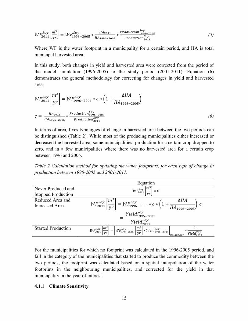
4.1.1 Climate Sensitivity

16

As previously mentioned, water footprint flow accounting is sensitive to uncertainties

related to precipitation, potential evapotranspiration, and temperature (Zhuo et al., 2014).

Adapting the results from (Mekonnen and Hoekstra, 2010) required first the analysis of

climatic changes between the two periods. Reanalysis gridded climate data for temperature

and precipitation were obtained from University of East Anglia Climatic Research Unit,

(2013) and analysed for the periods between 1995-2006 and 2001-2011.

Changes in the average precipitation and temperature for the two periods were calculated,

and a t-student test with 95% of significance level was applied to verify the significance of

these changes. Figure 2 shows the average temperature for the two periods (maps on the

right) and the difference between the two averages (map on the left); the area with

significant changes is highlighted with a dashed line. Figure 3 shows the average

precipitation for the two periods (maps on the right) and the difference between the two

averages (map on the left); the area with significant changes is highlighted with a dashed

line.

Figure 2 Difference between the medium temperatures in the two periods (left, %) with

significance level of 95% in t-student test (dashed line). Average temperature in the 1996-

-2005 period (above) and in the 2001-2011 period (below) (mm).

17

Even though by looking to the maps with the average temperature and precipitation for the

two periods it is difficult to visualize the differences between the two periods, the maps

with the difference between the averages demonstrate the regions with positive and

negative changes throughout the country. In terms of temperature, the area with significant

positive changes is located in the Amazon basin; this area is likely to have the footprints

slightly underestimated for the period of 2001-2011. The changes in precipitation, on the

other side, were not significant in most of the country apart from a small region in the south

of the country.

4.1.2 Production, Harvested Area and Yield Correction

The adaptation of the water footprint accounting valid for the period between 1996 and

2005 to the period between 2001 and 2011 will be possible by updating and adjusting the

parameters of yield, production and harvested area. The annual data on production, yield

Figure 3 Difference between the medium precipitations in the two periods (left, %) with

significance level of 95% in t-student test (dashed line). Average temperature in the

1996-2005 period (above) and in the 2001-2011 period (below) (mm).

18

and harvested area for each municipality were thus used as inputs to the equations

described in Table 2.

According to Table 2, the update of water footprint accounting from 1996-2005 to 2001-

2011 requires assessing the changes in production, harvested area and yield throughout

both periods. Figure 4 and Figure 5 demonstrate the changes in harvested area and

production, between 1996 and 2011, respectively. Although some municipalities presented

reduced production and harvested area, both had significant overall increase in the period

between 1996 and 2011.

Figure 4 Changes in harvested area between the two periods of 1996-2005 and 2001-2011

(left, %), and evolution of total harvested area in the entire country, from 1996-2011 (right,

Mtons).

Although a general upward trend can be observed in average yields (Figure 6), there is

great interannual variability in this period; the year of 2005 is specifically remarkable, with

a very sudden fall in yields to an average value below 2 tons of soy per hectare.

19

Figure 5 Changes in production between the two periods of 1996-2005 and 2001-2011

(left, %), and evolution of total in the entire country, from 1996-2011 (right, Mtons).

Figure 6 Changes in yield between 1996 and 2011 (left, ton/ha) and distribution of yield

values per municipality in the two periods: 1996-2005 (blue) and 2001-2011 (pink) (right).

By calculating the average production and harvested area for each municipality in both

periods, the municipalities were classified according to 5 typologies of production changes

(Figure 7). Soy production is widespread through the south and central-west regions of the

20

country; there is large expansion of soy production in the state of Mato Grosso, in the

boundaries between the Cerrado and Amazonian biomes (Lathuillière, 2011).

Figure 7 Distribution of the five typologies of changes in soy production between the

periods 1996-2005 and 2001-2011, per municipality.

4.2 WATER STRESS AND SCARCITY INDICATORS IN BRAZIL

A typology of water criticality was projected based on indicators of water scarcity, water

stress and agricultural water use. This classification made it possible to differentiate water

footprints from regions with different degrees of water stress, as well as to differentiate the

regions where the water stress was predominantly related to agriculture. First, the data used

to produce these indicators are described, as well as its source and estimation method.

Then, the methodology to calculate the three indicators will be described, and the matrix of

typologies is demonstrated.

4.2.1 Available Data

21

The water availability and water demand data were obtained from the Brazilian Water

Agency, and the population data was obtained from the National Institute of Geography and

Statistics (ANA, 2013; IBGE, 2011). In 2013 the Brazilian Water Agency (ANA) published

the Situation Analysis of Water Resources report, which evaluates the country’s water

resources in terms of availability, quality, multiple user demand, water conflict resolution

and governance (ANA, 2013). After the publication of this report, this extensive database

of water availability and demand estimated on the micro-basin scale for the entire country

was made available. The finer scale data has the spatial resolution of level 12 in the Otto

Pfapfstetter catchment coding system (Furnans and Olivera, 2001), which results in

168.843 polygons with average and maximum area of 5.071 and 371.245 hectares,

respectively.

The Brazilian Water Agency conceptualizes water demand as:

“Corresponds to the withdrawal flow, i.e., the water destined to meet diverse

consumptive uses. Part of this claimed water is given back to the environment

after use, which is denominated as return flow. (...) The non-return water, the

consumptive flow, is calculated as the difference between the water withdraw

and the return flow”. (Author’s translation, ANA, 2013, p. 87)

The water availability, on the other hand, is defined as the Q95%, i.e. the flow in cubic

metres per second which was equalled or exceeded for 95% of the flow record, summed to

the regularized flow, in case of existence of upstream dams.

The indicators of water availability, water demand and irrigated area were obtained in the

microbasin level, and were then regionalized to the municipality scale with the use of

Geographical Information System analysis. The indicators of water stress and irrigated area

index were calculated both for the municipal and microbasin scale, while water scarcity

was only estimated on the municipality scale, due to the use of municipal population data.

4.2.2 Water Stress, Scarcity and Irrigation Indicators

First, a water scarcity indicator based on the Falkenmark Scarcity Index was estimated, as

the quotient between the yearly available water in a certain area divided by the area’s

population. The water scarcity was classified according to the thresholds shown in Table 3

(Falkenmark and Widstrand, 1992; Falkenmark, 1986).

22

Table 3 Threshold levels for the Falkenmark scarcity indicator and Adapted Falkenmark

Scarcity Indicator (Falkenmark and Widstrand, 1992; Falkenmark, 1986; Adapted from

Perveen and James, 2011).

Falkenmark indicator for water

crowding (Persons per flow

unit/year)

‘Falkenmark indicator’

(m3/capita/year)

Water stress implication

>600 <1700 Water stress

>1000 <1000 Chronic water scarcity

>2000 <500 Beyond the water barrier

For estimation of water stress, a use-to-availability indicator was calculated, by dividing the

total water demand by the available water flow in the same area. Table 4 shows the

thresholds for each class of water stress, based on Raskin et al., (1996).

Table 4 Characterization of water stress use-to-availability ratio (adapted from Perveen

and James, 2011; Raskin et al., 1996)

Percent withdrawal Technical water stress

<10 Low water stress

10–20 Medium low water stress

20–40 Medium high water stress

>40 High water stress

An Irrigated Area Index was calculated based on the Equation (7) that uses as input the

actual percentage of irrigated area in the basin (%IArbasin), and the maximum and minimum

values for percentage of irrigated area per microbasin in the country (%IArmin, %IArmax).

𝑖𝐼𝐴𝑟% =(%𝐼𝐴𝑟𝑏𝑎𝑠𝑖𝑛)− (%𝐼𝐴𝑟𝑚𝑖𝑛)

(%𝐼𝐴𝑟𝑚𝑎𝑥)− (%𝐼𝐴𝑟𝑚𝑖𝑛) (7)

The classification of the area regarding the percentage of irrigated area is shown in Table 5.

Table 5 Classification microbasins according to an Irrigated Area Index.

Irrigated Area Index Irrigated area typology

iAIr= 0 a 0,333 Low

iAIr= 0,334 a 0,666 Medium

iAIr=0,667 a 1 High

4.2.3 Water Stress Typologies

The water criticality typology was classified according to the Table 6.

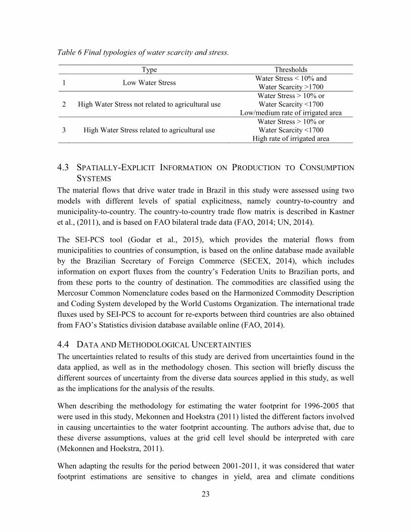
23

Table 6 Final typologies of water scarcity and stress.

Type Thresholds

1 Low Water Stress Water Stress < 10% and

Water Scarcity >1700

2 High Water Stress not related to agricultural use

Water Stress > 10% or

Water Scarcity <1700

Low/medium rate of irrigated area

3 High Water Stress related to agricultural use

Water Stress > 10% or

Water Scarcity <1700

High rate of irrigated area

4.3 SPATIALLY-EXPLICIT INFORMATION ON PRODUCTION TO CONSUMPTION

SYSTEMS

The material flows that drive water trade in Brazil in this study were assessed using two

models with different levels of spatial explicitness, namely country-to-country and

municipality-to-country. The country-to-country trade flow matrix is described in Kastner

et al., (2011), and is based on FAO bilateral trade data (FAO, 2014; UN, 2014).

The SEI-PCS tool (Godar et al., 2015), which provides the material flows from

municipalities to countries of consumption, is based on the online database made available

by the Brazilian Secretary of Foreign Commerce (SECEX, 2014), which includes

information on export fluxes from the country’s Federation Units to Brazilian ports, and

from these ports to the country of destination. The commodities are classified using the

Mercosur Common Nomenclature codes based on the Harmonized Commodity Description

and Coding System developed by the World Customs Organization. The international trade

fluxes used by SEI-PCS to account for re-exports between third countries are also obtained

from FAO’s Statistics division database available online (FAO, 2014).

4.4 DATA AND METHODOLOGICAL UNCERTAINTIES

The uncertainties related to results of this study are derived from uncertainties found in the

data applied, as well as in the methodology chosen. This section will briefly discuss the

different sources of uncertainty from the diverse data sources applied in this study, as well

as the implications for the analysis of the results.

When describing the methodology for estimating the water footprint for 1996-2005 that

were used in this study, Mekonnen and Hoekstra (2011) listed the different factors involved

in causing uncertainties to the water footprint accounting. The authors advise that, due to

these diverse assumptions, values at the grid cell level should be interpreted with care

(Mekonnen and Hoekstra, 2011).

When adapting the results for the period between 2001-2011, it was considered that water

footprint estimations are sensitive to changes in yield, area and climate conditions

24

(Mekonnen and Hoekstra, 2011; Zhuo et al., 2014). The methodology developed for

adaptation of the results described in section 4.1 aims to account for the changes in

production, yield and harvested area. Regarding climatic conditions, section 4.1.1 focused

on analyzing the areas in which the changes in average climatic condition were significant,

and could tamper with the final results. Figure 2 and Figure 3 show that, for most of the

country, the average climatic conditions were not significantly changed from one period to

the other. It is important to notice that, in the areas with significant changes, the results

should be interpreted with care; it should also be noted that the statistical variation in the

average climate is not necessarily an indicator of uncertainties in the climate variability in

these periods.

In the case of the trade data obtained from the SEI-PCS tool, the main source of

uncertainties are related to the quality of the data provided to the Brazilian government that

was obtained and processes, as well as regarding assumptions related to transport cost

optimization (Godar et al., 2015). The results were, however, validated through field

observations. Section 5.3 discusses the reasons why the allocation of Brazilian domestic

consumption is less reliable than international consumption allocation, and therefore why

this study analyzed only water footprints related to international consumers, and did not

address domestic consumption.

Finally, the water scarcity, water stress and irrigation information estimated by the

Brazilian Water Agency is subjected to two sources of uncertainty, related to the water

availability estimation, and to the valuation of water demands by total and irrigation uses.

The water availability values per microbasin are subjected to uncertainties resulting from

low density of hydrological stations for measurement of river flow, especially in the areas

in the North of the country. The water demands are estimated as a result of water permits

produced by the different water resource management institutions; it is, therefore, subjected

to underestimation of demand due to illegal water use (ANA, 2013).

5 RESULTS In this section, the assessment of water footprints of soy production in Brazil will be

presented through a variety of perspectives, according to the proposed methodology.

First, the raw footprint data from Mekonnen and Hoekstra, (2011) and bilateral trade flows

(Kastner et al., 2011) are coupled in order to assess Brazilian soy water footprints according

to the current footprint methodology. Subsequently, the coupling between the adapted

footprints for the 2001-2011 period and the spatially-explicit trade flow model (Godar et al.,

2015) offers an analysis of the geographical distribution of the water footprints and their

connection to global trade. Finally, these results are analysed in terms of regions with

different levels of water stress. The analysis of the case study of the Swedish footprints

provides context and exemplifies the outcomes of this research.

25

Table 7 summarizes all the results and their corresponding figures in terms of their

approach to water footprint accounting, trade flow, and classification of water stress.

Table 7 Summary of the water footprint results, and their approaches regarding WF

account, trade and water stress methodology.

Section Approach to WF

accounting Trade Flow

Classification of

Water Stress Figures

5.1

Results from

(Mekonnen and

Hoekstra, 2010)

(Kastner et al.,

2011) Aggregated

Figure 9 and Figure

8

5.2 Adapted WF

accounting

(Kastner et al.,

2011) Aggregated

Figure 10 and

Figure 11

5.3 Adapted WF

accounting

SEI-PCS (Godar

et al., 2015) Aggregated

Figure 12 to Figure

15

5.4 Adapted WF

accounting

SEI-PCS (Godar

et al., 2015) Disaggregated

Figure 22 to Figure

28

5.5 Adapted WF

accounting

SEI-PCS (Godar

et al., 2015) Disaggregated

Figure 29 to Figure

33

5.1 WATER FOOTPRINT ACCOUNTING: CURRENT APPROACH

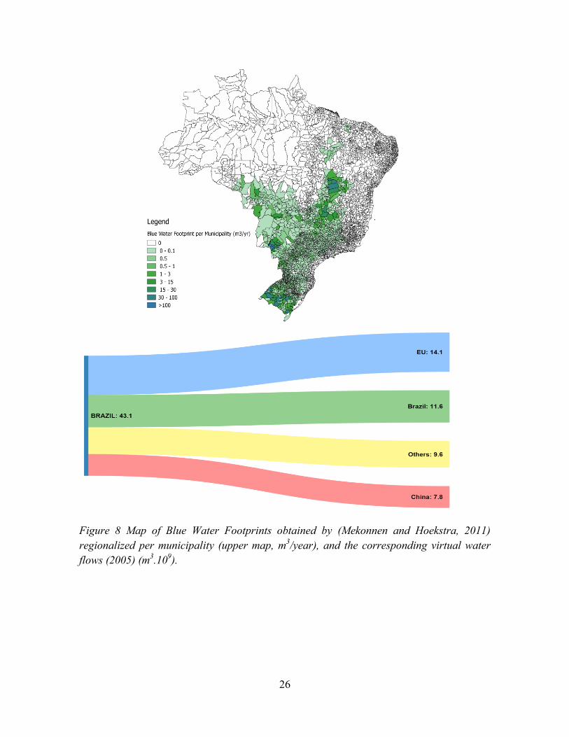
The assessment of water footprints using the results obtained in Mekonnen and Hoekstra,

(2011) and a country-to-country assessment of trade through a bilateral trade matrix

(Kastner et al., 2011) in the year of 2005 is exhibited in this section. The water footprint

estimates for soybeans according to Mekonnen and Hoekstra, (2011) (mm/year) were

obtained in raster format. These footprints were regionalized for the Brazilian

municipalities using GIS, and the result is presented in the upper right corner of Figure 9

(green water) and Figure 8 (blue water) (m3/year).

The Brazilian average soy green and blue water footprint between 1996-2005 was

estimated at 2181 and 0.8 m3.ton

-1 respectively (Mekonnen and Hoekstra, 2011). The blue

water footprint per ton of produce is much lower than the global average value of 70

m3.ton

-1, as a result of low levels of irrigated water use; the global average green water

footprint of 2037 m3.ton

-1, however, does not greatly diverge from the Brazilian values

(Mekonnen and Hoekstra, 2011).

Green water footprints are not only higher in overall values, but also have larger

geographical extension, as great parts of the country have predominantly rain-fed

agriculture. Higher values of blue water footprints are located in regions with both high

production and presence of irrigated agriculture, as is demonstrated by the geographical

distribution of footprints in the upper map of Figure 8 and Figure 9.

26

Figure 8 Map of Blue Water Footprints obtained by (Mekonnen and Hoekstra, 2011)


flows (2005) (m3.10

9).

27

The bottom part of Figure 8 and Figure 9 demonstrates the virtual water flows to the main

consumer regions in 2005: China, EU, Brazil and others. As the water footprint attributed

to each country is a function of the total footprints for that year and does not differentiate

the geographical location of that footprint, the values are linearly proportional to the

amount of soy attributed to the consumer. The sole highest consumer country is Brazil itself,

followed by China.

Figure 9 Map of Green Water Footprints obtained by (Mekonnen and Hoekstra, 2011)


flows (2005) (m3.10

9).

28

5.2 WATER FOOTPRINTS: ADAPTED ACCOUNTING

The results from the previous section were adapted to the period 2001-2011, following the

methodology described in section 4.1. Figure 10 presents the estimated average blue and

green water footprints for this period.

Figure 10 Average yearly blue (left, m3.10

6) and green (right, m

3.10

9) water footprints per

municipality for the period between 2001 and 2011.

The virtual water fluxes for 2005 based by the adaptation of the model results resulted in

values higher than the ones estimated for the same year, with the previous results. This is

due to variations in yield, production and harvested area from year to year; as can be

observed in section 4.1.2, a dramatic decrease in yield was observed in 2005, resulting in

higher values of both green and blue water footprints. As the fluxes were also based on

country-to-country trade matrices, the relative attribution of footprints to the consumer

regions remains the same, as it is proportional to the amount of soy consumed by each

consumer region (Figure 11).

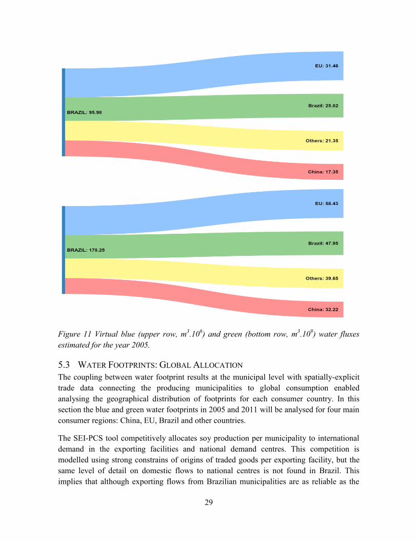
29

Figure 11 Virtual blue (upper row, m3.10

6) and green (bottom row, m

3.10

9) water fluxes

estimated for the year 2005.

5.3 WATER FOOTPRINTS: GLOBAL ALLOCATION

The coupling between water footprint results at the municipal level with spatially-explicit

trade data connecting the producing municipalities to global consumption enabled

analysing the geographical distribution of footprints for each consumer country. In this

section the blue and green water footprints in 2005 and 2011 will be analysed for four main

consumer regions: China, EU, Brazil and other countries.

The SEI-PCS tool competitively allocates soy production per municipality to international

demand in the exporting facilities and national demand centres. This competition is

modelled using strong constrains of origins of traded goods per exporting facility, but the

same level of detail on domestic flows to national centres is not found in Brazil. This

implies that although exporting flows from Brazilian municipalities are as reliable as the

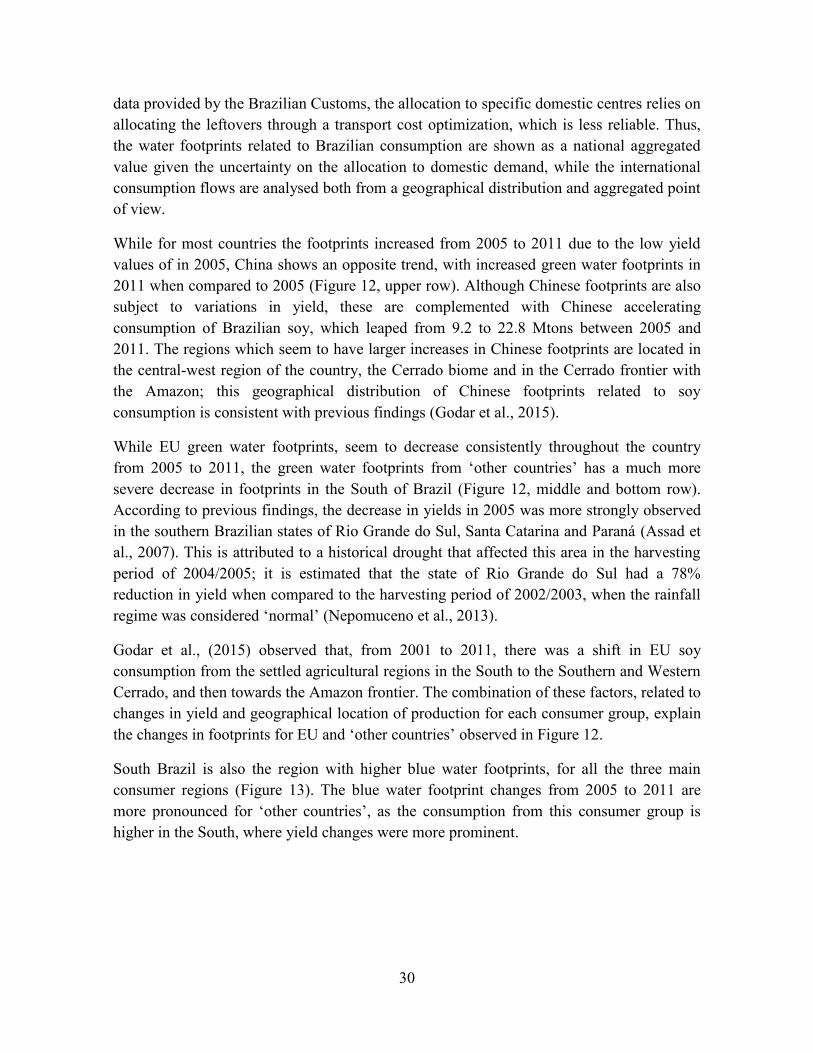
30

data provided by the Brazilian Customs, the allocation to specific domestic centres relies on

allocating the leftovers through a transport cost optimization, which is less reliable. Thus,

the water footprints related to Brazilian consumption are shown as a national aggregated

value given the uncertainty on the allocation to domestic demand, while the international

consumption flows are analysed both from a geographical distribution and aggregated point

of view.

While for most countries the footprints increased from 2005 to 2011 due to the low yield

values of in 2005, China shows an opposite trend, with increased green water footprints in

2011 when compared to 2005 (Figure 12, upper row). Although Chinese footprints are also

subject to variations in yield, these are complemented with Chinese accelerating

consumption of Brazilian soy, which leaped from 9.2 to 22.8 Mtons between 2005 and

2011. The regions which seem to have larger increases in Chinese footprints are located in

the central-west region of the country, the Cerrado biome and in the Cerrado frontier with

the Amazon; this geographical distribution of Chinese footprints related to soy

consumption is consistent with previous findings (Godar et al., 2015).

While EU green water footprints, seem to decrease consistently throughout the country

from 2005 to 2011, the green water footprints from ‘other countries’ has a much more

severe decrease in footprints in the South of Brazil (Figure 12, middle and bottom row).

According to previous findings, the decrease in yields in 2005 was more strongly observed

in the southern Brazilian states of Rio Grande do Sul, Santa Catarina and Paraná (Assad et

al., 2007). This is attributed to a historical drought that affected this area in the harvesting

period of 2004/2005; it is estimated that the state of Rio Grande do Sul had a 78%

reduction in yield when compared to the harvesting period of 2002/2003, when the rainfall

regime was considered ‘normal’ (Nepomuceno et al., 2013).

Godar et al., (2015) observed that, from 2001 to 2011, there was a shift in EU soy

consumption from the settled agricultural regions in the South to the Southern and Western

Cerrado, and then towards the Amazon frontier. The combination of these factors, related to

changes in yield and geographical location of production for each consumer group, explain

the changes in footprints for EU and ‘other countries’ observed in Figure 12.

South Brazil is also the region with higher blue water footprints, for all the three main

consumer regions (Figure 13). The blue water footprint changes from 2005 to 2011 are

more pronounced for ‘other countries’, as the consumption from this consumer group is

higher in the South, where yield changes were more prominent.

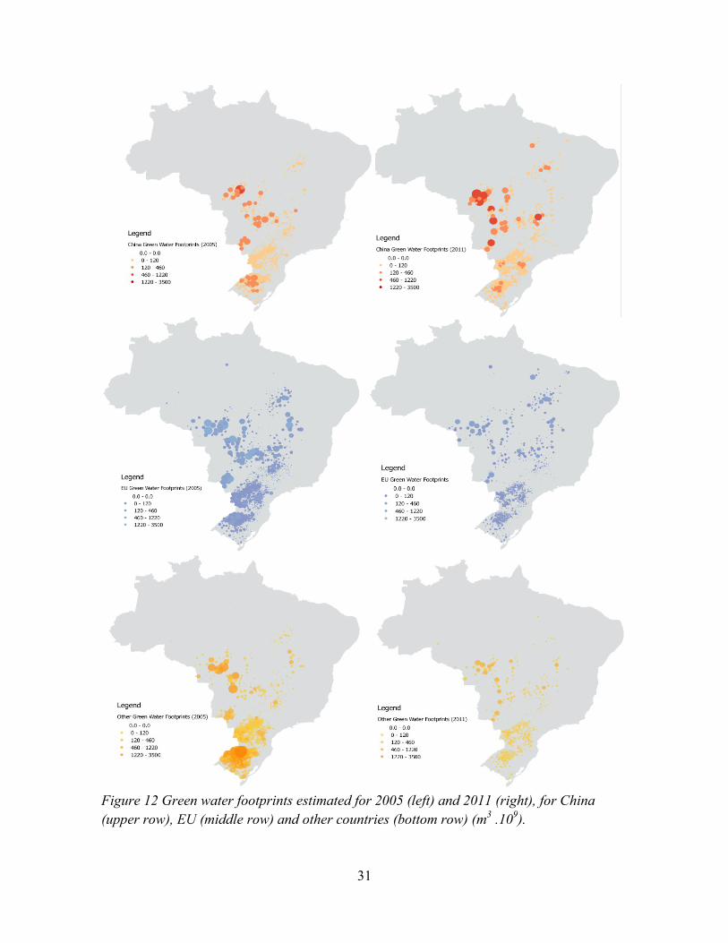
31

Figure 12 Green water footprints estimated for 2005 (left) and 2011 (right), for China

(upper row), EU (middle row) and other countries (bottom row) (m3 .10

9).

32

Figure 13 Blue water footprints estimated for 2005 (left) and 2011 (right), for China (upper

row), EU (middle row) and other countries (bottom row) (m3.10

6).

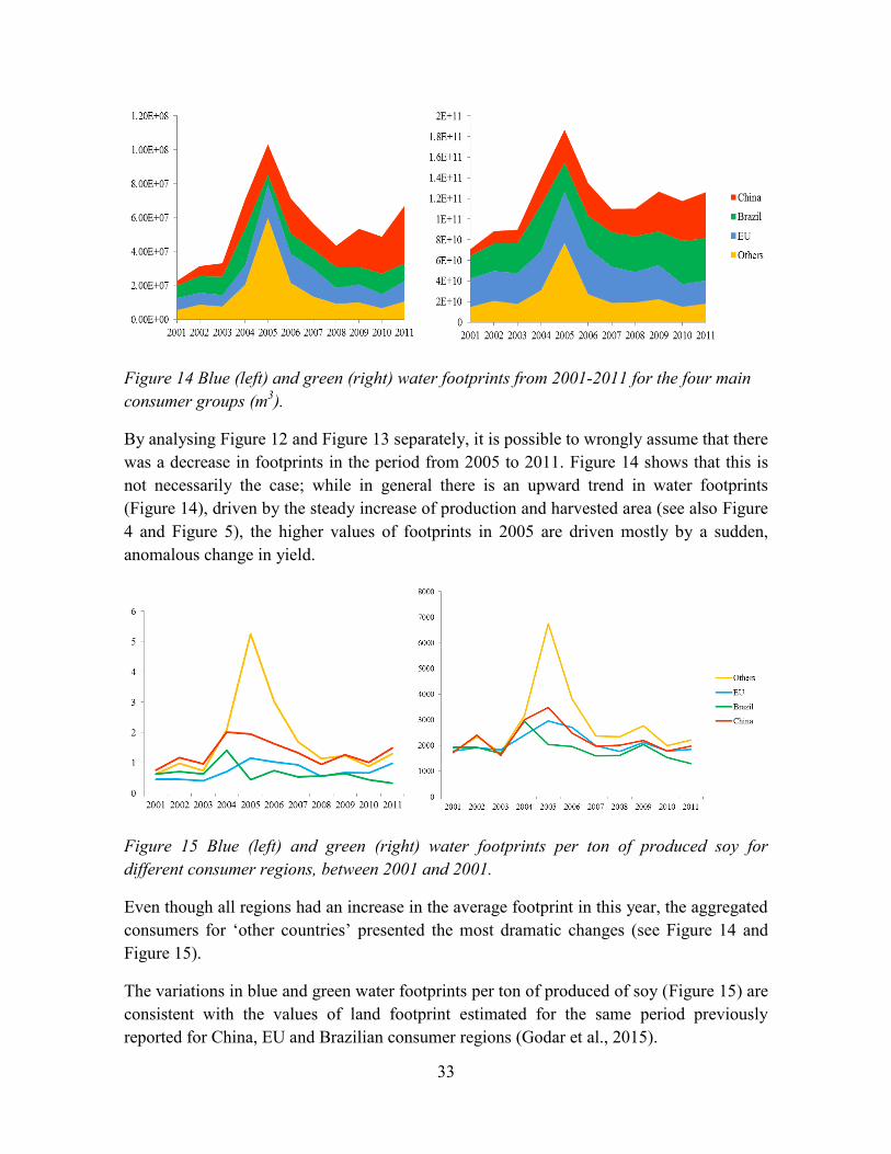
33

Figure 14 Blue (left) and green (right) water footprints from 2001-2011 for the four main

consumer groups (m3).

By analysing Figure 12 and Figure 13 separately, it is possible to wrongly assume that there

was a decrease in footprints in the period from 2005 to 2011. Figure 14 shows that this is

not necessarily the case; while in general there is an upward trend in water footprints

(Figure 14), driven by the steady increase of production and harvested area (see also Figure

4 and Figure 5), the higher values of footprints in 2005 are driven mostly by a sudden,

anomalous change in yield.

Figure 15 Blue (left) and green (right) water footprints per ton of produced soy for

different consumer regions, between 2001 and 2001.

Even though all regions had an increase in the average footprint in this year, the aggregated

consumers for ‘other countries’ presented the most dramatic changes (see Figure 14 and

Figure 15).

The variations in blue and green water footprints per ton of produced of soy (Figure 15) are

consistent with the values of land footprint estimated for the same period previously

reported for China, EU and Brazilian consumer regions (Godar et al., 2015).

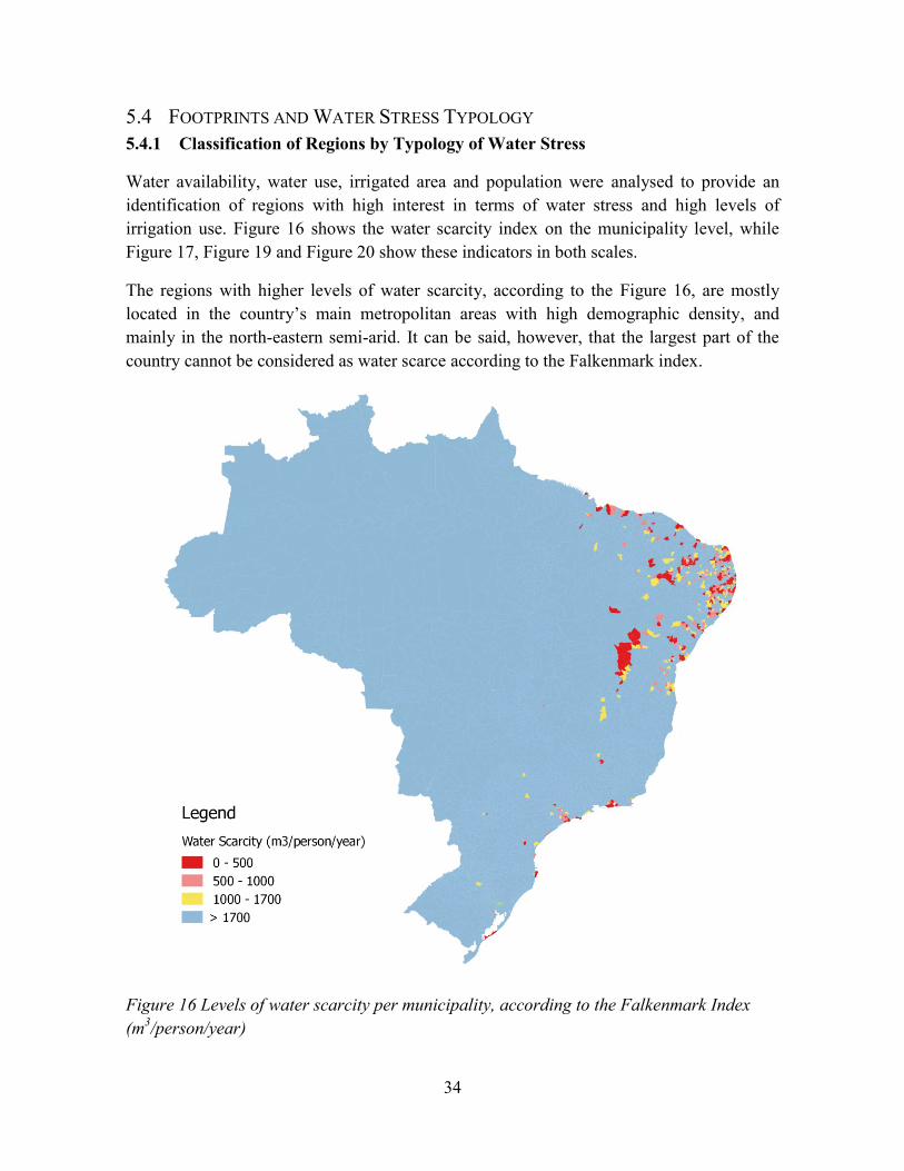
34

5.4 FOOTPRINTS AND WATER STRESS TYPOLOGY

5.4.1 Classification of Regions by Typology of Water Stress

Water availability, water use, irrigated area and population were analysed to provide an

identification of regions with high interest in terms of water stress and high levels of

irrigation use. Figure 16 shows the water scarcity index on the municipality level, while

Figure 17, Figure 19 and Figure 20 show these indicators in both scales.

The regions with higher levels of water scarcity, according to the Figure 16, are mostly

located in the country’s main metropolitan areas with high demographic density, and

mainly in the north-eastern semi-arid. It can be said, however, that the largest part of the

country cannot be considered as water scarce according to the Falkenmark index.

Figure 16 Levels of water scarcity per municipality, according to the Falkenmark Index

(m3/person/year)

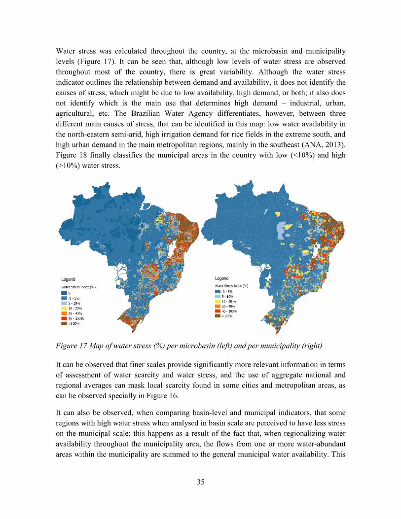
35

Water stress was calculated throughout the country, at the microbasin and municipality

levels (Figure 17). It can be seen that, although low levels of water stress are observed

throughout most of the country, there is great variability. Although the water stress

indicator outlines the relationship between demand and availability, it does not identify the

causes of stress, which might be due to low availability, high demand, or both; it also does

not identify which is the main use that determines high demand – industrial, urban,

agricultural, etc. The Brazilian Water Agency differentiates, however, between three

different main causes of stress, that can be identified in this map: low water availability in

the north-eastern semi-arid, high irrigation demand for rice fields in the extreme south, and

high urban demand in the main metropolitan regions, mainly in the southeast (ANA, 2013).

Figure 18 finally classifies the municipal areas in the country with low (<10%) and high

(>10%) water stress.

It can be observed that finer scales provide significantly more relevant information in terms

of assessment of water scarcity and water stress, and the use of aggregate national and

regional averages can mask local scarcity found in some cities and metropolitan areas, as

can be observed specially in Figure 16.

It can also be observed, when comparing basin-level and municipal indicators, that some

regions with high water stress when analysed in basin scale are perceived to have less stress

on the municipal scale; this happens as a result of the fact that, when regionalizing water

availability throughout the municipality area, the flows from one or more water-abundant

areas within the municipality are summed to the general municipal water availability. This

Figure 17 Map of water stress (%) per microbasin (left) and per municipality (right)

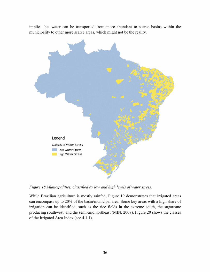
36

implies that water can be transported from more abundant to scarce basins within the

municipality to other more scarce areas, which might not be the reality.

Figure 18 Municipalities, classified by low and high levels of water stress.

While Brazilian agriculture is mostly rainfed, Figure 19 demonstrates that irrigated areas

can encompass up to 20% of the basin/municipal area. Some key areas with a high share of

irrigation can be identified, such as the rice fields in the extreme south, the sugarcane

producing southwest, and the semi-arid northeast (MIN, 2008). Figure 20 shows the classes

of the Irrigated Area Index (see 4.1.1).

37

The distribution of the final typology of water stress according to the classification

described in Section 4.1.1 is outlined in Figure 21. Out of 5570 Brazilian municipalities,

1195 (21%) were classified with high water stress and irrigation rates, 618 (11%) with

water stress with low rates of irrigation, and the remaining 3748 were classified as with low

levels of water stress.

Figure 19 Irrigated area, as a percentage of the total area of the microbasin (left) and

municipality (right).

Figure 20 Irrigated Area Index, by microbasin (left) and by municipality (right).

38

Figure 21 Final typologies for stress and irrigation, to be applied in the study.

The geographical distribution of the regions with high water stress are the same as in Figure

16 and Figure 18, with the regions of stress mainly concentrated in the highly irrigated

agriculture in the south, the semi-arid north-east and densely populated metropolitan

regions; in Figure 21 it is possible, however, to identify the regions with high water stress

that have irrigation infrastructure, such as in the extreme south, north-eastern coast, and in

the regions located close to the São Francisco river. Figure 21 also identifies the numbers

and colours that will identify each typology in the following sections.

5.4.2 Water Footprints Classified by Stress Typologies

This section presents the results shown in Section 5.3 classified according to the typologies

of water stress defined by the methodology chosen. The patterns blue and green water

footprints were analysed in terms of their temporal and geographical variations for the main

consumer regions. The regions with water stress that are mainly not related to agricultural

water use have comparatively small overall blue and green water footprints; even though

this class represents 11% of the municipalities (Figure 21), its total footprints are nearly

negligible (Figure 22), and the sum of the footprints in these regions consistently make up

to less than 2% of the total footprints (Figure 23).

39

Figure 22 Blue (left) and green (right) water footprints between 2001 and 2011, by


water stress, irrigation (3, green).

Figure 23 Proportion of blue (left) and green (right) water footprints per water stress

typology region between 2001 and 2011 (%): low water stress (1, blue); high water stress

(2, red); high water stress, irrigation (3, green)

40

It can be assumed that these municipalities are either subjected to economic and climatic

conditions that result in inadequacy for large-scale soy production, or have high water

demands for urban supply or industry, which characterizes areas with diversified

economical activities and resulting low levels of agricultural production.

It is self-evident that highly irrigated areas might represent a larger share of blue water

footprints when compared to their share of green water footprints (Figure 22). The ratio

between blue water footprints in terms of their typology, however, varies with time (Figure

23). These variations are a result of the geographical distribution of changes in production

and yield.

Analyzing the comparison between Chinese water footprints in Figure 24 and Figure 25 it

is evident that there is an increase of virtual water flows in this period, which is driven by

the steady increase of Chinese demand for Brazilian soy, especially from the regions

located in the Center-West and North of the country. The water footprints related to EU and

other countries’ consumption are also increasing, but in a much less dramatic way.

41

Figure 24 Blue water footprints for China (upper row), EU (middle row) and other


2011 (right).

42

Figure 25 Green water footprints for China (upper row), EU (middle row) and other


2011 (right).

43

Figure 26 Blue (left) and green (right) water footprints (m³) for China (upper row), EU

(middle row) and other countries (bottom row), classified by water stress typology, for the

years between 2001 and 2011.

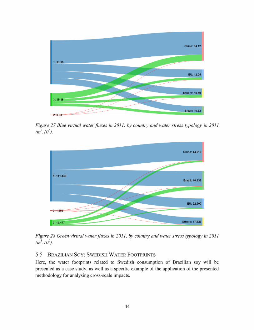
44

Figure 27 Blue virtual water fluxes in 2011, by country and water stress typology in 2011

(m3.10

6).

Figure 28 Green virtual water fluxes in 2011, by country and water stress typology in 2011

(m3.10

9).

5.5 BRAZILIAN SOY: SWEDISH WATER FOOTPRINTS

Here, the water footprints related to Swedish consumption of Brazilian soy will be

presented as a case study, as well as a specific example of the application of the presented

methodology for analysing cross-scale impacts.

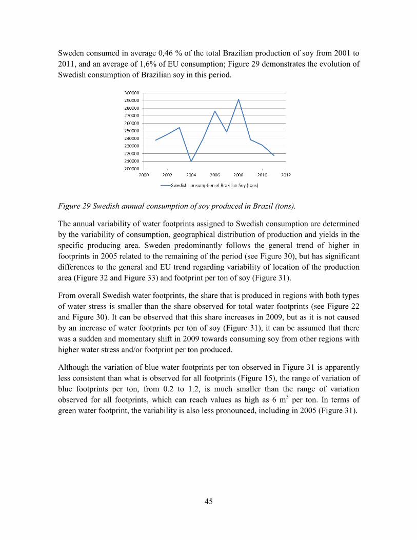
45

Sweden consumed in average 0,46 % of the total Brazilian production of soy from 2001 to

2011, and an average of 1,6% of EU consumption; Figure 29 demonstrates the evolution of

Swedish consumption of Brazilian soy in this period.

Figure 29 Swedish annual consumption of soy produced in Brazil (tons).

The annual variability of water footprints assigned to Swedish consumption are determined

by the variability of consumption, geographical distribution of production and yields in the

specific producing area. Sweden predominantly follows the general trend of higher in

footprints in 2005 related to the remaining of the period (see Figure 30), but has significant

differences to the general and EU trend regarding variability of location of the production

area (Figure 32 and Figure 33) and footprint per ton of soy (Figure 31).

From overall Swedish water footprints, the share that is produced in regions with both types

of water stress is smaller than the share observed for total water footprints (see Figure 22

and Figure 30). It can be observed that this share increases in 2009, but as it is not caused

by an increase of water footprints per ton of soy (Figure 31), it can be assumed that there

was a sudden and momentary shift in 2009 towards consuming soy from other regions with

higher water stress and/or footprint per ton produced.

Although the variation of blue water footprints per ton observed in Figure 31 is apparently

less consistent than what is observed for all footprints (Figure 15), the range of variation of

blue footprints per ton, from 0.2 to 1.2, is much smaller than the range of variation

observed for all footprints, which can reach values as high as 6 m3 per ton. In terms of

green water footprint, the variability is also less pronounced, including in 2005 (Figure 31).

46


typology of water stress (m3).


typology of water stress, per ton of produced soy (m3/ton).

The regions where the soy consumed in Sweden is produced are mostly located in the

north-west region of the State of Paraná, south of Mato Grosso do Sul and mainly in Mato

Grosso (center-west part of the country). The low dependency on soy from the South made

the variation of footprints in 2005 for Sweden less pronounced than for other countries;

most of the blue water footprint in 2005 is from the north of the State of Paraná, which was

also influenced by the drought, but in a smaller extent.

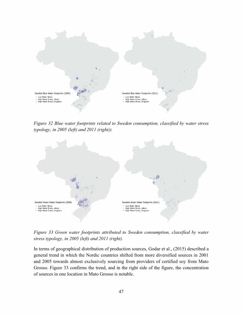
47

Figure 32 Blue water footprints related to Sweden consumption, classified by water stress

typology, in 2005 (left) and 2011 (right)).

Figure 33 Green water footprints attributed to Sweden consumption, classified by water

stress typology, in 2005 (left) and 2011 (right).

In terms of geographical distribution of production sources, Godar et al., (2015) described a

general trend in which the Nordic countries shifted from more diversified sources in 2001

and 2005 towards almost exclusively sourcing from providers of certified soy from Mato

Grosso. Figure 33 confirms the trend, and in the right side of the figure, the concentration

of sources in one location in Mato Grosso is notable.

48

6 DISCUSSION AND CONCLUDING REMARKS The results provided insight on the processes that connect the water cycle in Brazilian

locations to the global market and the global water system between 2001 and 2011, and

how this relationship is established with different actors. First, the methodological aspects

related to this study will be discussed, in terms of applicability and relevance for decision

making. Then, some aspects related to the analysis of green and blue water sustainability on

the local scale will be addressed. The relevance of the results in the context of

teleconnections within the global water system will be discussed and, finally, a description

and discussion of the opportunities for future research are presented.

6.1 PROPOSED APPROACH TO WATER FOOTPRINT ACCOUNTING:

IMPROVEMENTS AND ADDED KNOWLEDGE

The analysis of the geographical distribution and environmental relevance of footprints

attributed to main consumers of Brazilian soy has allowed to unveil environmental trade-

offs which could not be observed with the use of country aggregates, that can mask

temporal and geographical variability of production conditions and potential impacts in the

local scale. The methodological approach described and developed in this study improves

other footprint assessments as the spatial-explicit trade analysis and assessment of local

impacts allowed three important factors to be addressed, namely i) the ultimate drivers of

pressure from the global food system, ii) the local environmental and social impacts related

to the water footprints, and iii) the connection between them.

As it was perceived in the analysis of the distribution of footprints by consumer region,

total and relative virtual water flows are determined not only by the local production

conditions, but also by distribution of production that is a result of a series of the remote

drivers that include prices, logistics, competition, institutional agreements, technological

changes, among others (Wichelns, 2010). In the case of Brazilian soy production, the

growing demand of the international market have driven a shift towards water and soil rich

regions in the Cerrado and Amazon biomes, mainly by consumers from Chinese and EU

markets (Godar et al., 2015; Lathuillière et al., 2014). This shift has also been related to an

increase of deforestation in these areas (Lathuillière, 2011; Persson et al., 2014), as well as

an increase in the green water footprint from those regions (see Figure 12). On the other

side, the sourcing of smaller consumers predominantly from the southern regions with

long-settled agriculture and irrigation structure resulted in a larger impact of the drought of

2005 on the footprints related to these consumers.

This exemplifies that local aspects of water management and land use change decision

making, climatic conditions, productivity improvement, among others, constitute the

drivers of impact at the local scale.

49

In the case of the analysed context of Brazilian soy production, the contrast between the

different contexts of the South and the North constitutes a good example of why the spatial-

explicitness of the analysis is fundamental for the understanding of the relationship between

the main drivers of change and local impacts. These regions have very different profiles of

consumers, profiles of green/blue water dependency, and conflicts over resource use and

socio-economic impacts. Analysing water footprints from Brazilian soy in terms of national

aggregates, such as what is done in the section 5.1, provides with an idea of flows and

impacts, but mask regional differences such as the ones described.

6.2 ASSESSMENT OF BLUE AND GREEN WATER SUSTAINABILITY

As was summarized previously in this study, there is a rich debate on how to analyse water

footprint accounting results, and where their relevance lies. It can be argued that larger

footprints do not necessarily equal to larger impacts in the local water system, as the key to

understanding them is their environmental and social relevance (Ridoutt and Huang, 2012).

The indicators and typologies of water stress used in this study were chosen with the

objective to measure the sustainability of water footprints in terms of their contribution to

scarcity and competing pressures over water resources at the local level. Other options of

analysis include consideration of impacts to ecosystems, contributions of land use change

in changes of moisture transport, green water feedbacks, among others (Lathuillière et al.,

2014; Quinteiro et al., 2015; Vörösmarty et al., 2010).

Another important distinction that needs to be considered when analysing the results of the

study is that the indicators of stress employed for classification of water footprints focused

in blue water scarcity. Blue water is central in terms of water security for human supply,

and the analysis of these indicators provide important information on the local pressure

over resources and threats related to water scarcity. Although pressures on green water

were not considered in this study, both green and blue water footprints were aggregated

according to the blue water stress in the region of interest. The analysis of blue and green

water footprints in the context of the water stress typologies should be done with

consideration to their different nature.

The blue water footprint impacts directly availability of water for other downstream users,

and is a part of the competing demands for resources in the local scale. The analysis of the

blue water footprints in this context is done, therefore, from a point of view of resource

competition and scarcity avoidance. Therefore, in the regions with high blue water

footprints located in regions with high levels of water stress, the water footprint connected

to commodity production constitutes a competing demand for resources, which can evolve

into water conflicts in situations of scarcity. One example was the drought of 2005, when

410 municipalities declared situation of emergency, and measures such as forceful sealing

of irrigation pumps were taken (Germano and Sotério, 2005).

50

In terms of green water footprints, the amount of virtual trade flows can be considered in

terms of resource dependency and vulnerability. It is theorized that international trade of

virtual water compensates regional differences in water availability (Konar et al., 2013); as

green water becomes available for food production through land use change (Ridoutt and

Pfister, 2010), the green water footprint is also a measure of dependency on external

availability of water and land. One example is the increasing dependency of Chinese

demand of soy expanding in the Amazon and Cerrado biomes, which is expected to

increase in the years to come.

6.3 GLOBAL TRADE, LOCAL IMPACTS

The approach to water footprints, trade and water stress developed in this study can greatly

improve the understanding of the linkages between dynamics of consumption, trade and

production systems in the context of water pressures, contributing to improve governance

and policies. This section will address how this approach could potentially improve the

scope of analysis or serve as a basis for more policy relevant results studies related to

global food security, international competition over resources, consumption responsibility,

or local water governance.

Studies have tried to analyse the impacts of future climate on rainfed agriculture and global

food security, and the cross-scale vulnerabilities related to these processes (Falkenmark and

A, 2013; Rockström et al., 2009; Willaarts et al., 2015). It is expected that, under climate

change, food security will face major challenges (Allouche, 2011). In Brazil, the main

regions of soy production for international consumption in the Amazon/Cerrado and in the

La Plata Basin are, respectively, increasingly subjected to shifts in local precipitation

regime due to land use change (Nobre, 2014) and climate extremes related to interannual

variability and climate change (Cavalcanti et al., 2015). The analysis of green virtual water

trade and the connection with local conditions of water stress, as the one developed in this

study, can provide new paths of investigation.

The results presented also indicate another perspective of analysis regarding how

competition over resources takes shape in the international commodity markets. In the

example of Brazilian Soy, it was seen that i) the larger consumers shifted towards new sites

of production, but with greater impacts on land use change; ii) that the positioning of other

smaller consumer markets resulted in the fact that they were subjected more strongly to an

episode of climate extremes; and ii) that a small but powerful and environmentally

conscious consumer like Sweden guaranteed a share of the market to supply soy of certified

origin. Whether these patterns are planned or driven by other social, economic or logistic

factors, they determine different access to resources in the short and long term. The

distribution of these footprints and analysis of trade-offs and impacts could only be possible

with spatially-explicit footprint analysis of these socio-economic systems.

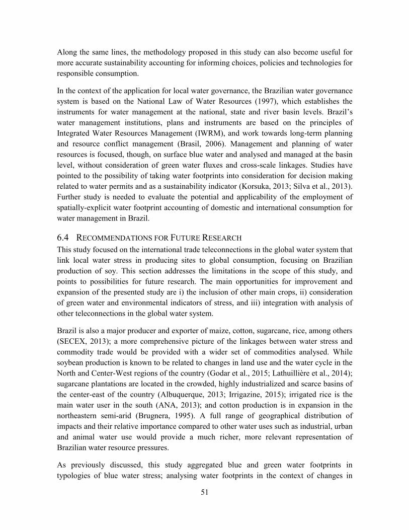
51

Along the same lines, the methodology proposed in this study can also become useful for

more accurate sustainability accounting for informing choices, policies and technologies for

responsible consumption.

In the context of the application for local water governance, the Brazilian water governance

system is based on the National Law of Water Resources (1997), which establishes the

instruments for water management at the national, state and river basin levels. Brazil’s

water management institutions, plans and instruments are based on the principles of

Integrated Water Resources Management (IWRM), and work towards long-term planning

and resource conflict management (Brasil, 2006). Management and planning of water

resources is focused, though, on surface blue water and analysed and managed at the basin

level, without consideration of green water fluxes and cross-scale linkages. Studies have

pointed to the possibility of taking water footprints into consideration for decision making

related to water permits and as a sustainability indicator (Korsuka, 2013; Silva et al., 2013).

Further study is needed to evaluate the potential and applicability of the employment of

spatially-explicit water footprint accounting of domestic and international consumption for

water management in Brazil.

6.4 RECOMMENDATIONS FOR FUTURE RESEARCH

This study focused on the international trade teleconnections in the global water system that

link local water stress in producing sites to global consumption, focusing on Brazilian

production of soy. This section addresses the limitations in the scope of this study, and

points to possibilities for future research. The main opportunities for improvement and

expansion of the presented study are i) the inclusion of other main crops, ii) consideration

of green water and environmental indicators of stress, and iii) integration with analysis of

other teleconnections in the global water system.

Brazil is also a major producer and exporter of maize, cotton, sugarcane, rice, among others

(SECEX, 2013); a more comprehensive picture of the linkages between water stress and

commodity trade would be provided with a wider set of commodities analysed. While

soybean production is known to be related to changes in land use and the water cycle in the

North and Center-West regions of the country (Godar et al., 2015; Lathuillière et al., 2014);

sugarcane plantations are located in the crowded, highly industrialized and scarce basins of

the center-east of the country (Albuquerque, 2013; Irrigazine, 2015); irrigated rice is the

main water user in the south (ANA, 2013); and cotton production is in expansion in the

northeastern semi-arid (Brugnera, 1995). A full range of geographical distribution of

impacts and their relative importance compared to other water uses such as industrial, urban

and animal water use would provide a much richer, more relevant representation of

Brazilian water resource pressures.

As previously discussed, this study aggregated blue and green water footprints in

typologies of blue water stress; analysing water footprints in the context of changes in

52

green water fluxes are an important opportunity of improvement. There is a growing

literature on methodological aspects for analysis of green water fluxes as a result of land

use change, and the use of these assessments as indicators of sustainability (Lathuillière et

al., 2014; Quinteiro et al., 2015).

Finally, a promising step for future research is to involve the assessment of teleconnections

in the global water system through trade, such as the present study, with assessment of

other remote connections that operate in the same systems. Combining the assessment of

crop production and trade with the estimations of green water flux change due to

agriculture and land use change (Lathuillière et al., 2014) and intercontinental moisture

transport (Keys et al., 2012) can allow to reveal trade-offs in the water system in a much

wider scope and scale.

53

7 ACKNOWLEDGEMENTS In the process of developing this Thesis, I was incredibly lucky to have the guidance and

supervision of Tina, in Linköping University, and Javier, in the Stockholm Environment

Institute. I would like to express my gratitude to Tina, for the patience and support.

I am very thankful to Javier, who kindly accepted to be me as part of his team, and gave me

the opportunity to join an extraordinarily rich and diverse environment in SEI; these last

couple of months have been an incredible learning experience. Your advice and mentorship,

always challenging and motivating, have been a great inspiration for me, both personally

and professionally. In SEI, I would also like to thank Toby and Louise for the guidance and

very interesting inputs, as well as James and Kate, for the fikas and instant companionship.

To all of my friends and professors in Linköping, who made these two last years an

unforgettable experience, my truthful appreciation.

I would like to finally express my most heartfelt thanks to Jonas, who regardless of the

distance is my most honest, optimist and loving cheerleader. Your passion, dedication, and

drive to make a difference have always been a great inspiration for me to do my best.

This publication has been produced during my scholarship period at Linköping University,

thanks to a Swedish Institute scholarship.

54

8 REFERENCES

Albuquerque, M.F. de, 2013. Medições e Modelagem da Pegada Hídrica da Cana-de-

Açucar Cultivada no Brasil. Universidade Federal de Campina Grande.

Allouche, J., 2011. The sustainability and resilience of global water and food systems:

Political analysis of the interplay between security, resource scarcity, political systems

and global trade. Food Policy 36, S3–S8. doi:10.1016/j.foodpol.2010.11.013

Alvarenga, R.A.F. De, da Silva Júnior, V.P., Soares, S.R., 2012. Comparison of the

ecological footprint and a life cycle impact assessment method for a case study on

Brazilian broiler feed production. J. Clean. Prod. 28, 25–32.

doi:10.1016/j.jclepro.2011.06.023

ANA, 2013. Conjuntura dos Recursos Hídricos no Brasil 2013. Brasilia.

Ansink, E., 2010. Refuting two claims about virtual water trade. Ecol. Econ. 69, 2027–

2032. doi:10.1016/j.ecolecon.2010.06.001

Assad, E.D., Marin, F.R., Evangelista, S.R., Pilau, F.G., Farias, J.R.B., Pinto, H.S., Zullo,

J., 2007. Sistema de previsão da safra de soja para o Brasil. Pesqui. Agropecu. Bras.

42, 615–625. doi:10.1590/S0100-204X2007000500002

Brasil, 2006. Plano Nacional de Recursos Hídricos. Brasília.

Brasil, 2008. Plano Nacional Sobre Mudança do Clima - PNMC.

Brown-Lima, C., Cooney, M., Cleary, D., 2009. An overview of the Brazil-China soybean

trade and its strategic implications for conservation. United States Agency Int. Dev.

Brugnera, P., 1995. Irrigação do Algodoeiro no Cerrado Baiano, in: V Congresso Brasileiro

de Algodão. EMBRAPA, Salvador.

Carmo, R.L. Do, Ojima, A.L.R.D.O., Ojima, R., Nascimento, T.T. Do, 2007. Água virtual,

escassez e gestão: o Brasil como grande “exportador” de água. Ambient. Soc. 10, 83–

96. doi:10.1590/S1414-753X2007000200006

Cavalcanti, I.F.A., Carril, A.F., Penalba, O.C., Grimm, A.M., Menéndez, C.G., Sanchez, E.,

Cherchi, A., Sörensson, A., Robledo, F., Rivera, J., Pántano, V., Bettolli, L.M.,

Zaninelli, P., Zamboni, L., Tedeschi, R.G., Dominguez, M., Ruscica, R., Flach, R.,

2015. Precipitation extremes over La Plata Basin – Review and new results from

observations and climate simulations. J. Hydrol. 523, 211–230.

doi:10.1016/j.jhydrol.2015.01.028

55

Chapagain, A.K., Hoekstra, a. Y., Savenije, H.H.G., 2006. Water saving through

international trade of agricultural products. Hydrol. Earth Syst. Sci. 10, 455–468.

doi:10.5194/hess-10-455-2006

Chen, Z.-M., Chen, G.Q., 2013. Virtual water accounting for the globalized world

economy: National water footprint and international virtual water trade. Ecol. Indic.

28, 142–149. doi:10.1016/j.ecolind.2012.07.024

Ercin, a E., Hoekstra, A.Y., 2012. Carbon and Water Footprints: Concepts, Methodologies

and Policy Responses.

Ercin, a E., Hoekstra, A.Y., 2014. Water footprint scenarios for 2050: a global analysis.

Environ. Int. 64, 71–82. doi:10.1016/j.envint.2013.11.019

Falkenmark, M., 1986. Fresh Water-Time: For A Modified Approach. Ambio 15, 192–200.

doi:10.2307/4313251

Falkenmark, M., A, P.T.R.S., 2013. Growing water scarcity in agriculture : future challenge

to global water security. Phil Trans R Soc A 371, 14.

Falkenmark, M., Berntell, A., Jägerskog, A., Lundqvist, J., Matz, M., Tropp, H., 2007. On

the Verge of a New Water Scarcity: A Call for Good Governance and Human

Ingenuity.

Falkenmark, M., Rockström, J., 2010. Building water resilience in the face of global

change: from a blue-only to a green-blue water approach to land-water management. J.

Water Resour. Plan. Manag. 606–611.

Falkenmark, M., Widstrand, C., 1992. Population and water resources : a delicate balance.,

Population bulletin: 47:3. Washington, D.C. : Population Reference Bureau, 1992.

Fao, 2008. Example of the use of cropwat 8.0 1–75.

FAO, 2014. FAOSTAT Statistical Database [WWW Document]. URL http://data.fao.org/

Feng, K., Hubacek, K., Minx, J., Siu, Y.L., Chapagain, A.K., Yu, Y., Guan, D., Barrett, J.,

2010. Spatially Explicit Analysis of Water Footprints in the UK. Water 3, 47–63.

doi:10.3390/w3010047

Furnans, J., Olivera, F., 2001. Watershed Topology - The Pfafstetter System. Esri User

Conf.

Galli, A., Wiedmann, T., Ercin, E., Knoblauch, D., Ewing, B., Giljum, S., 2012. Integrating

Ecological, Carbon and Water footprint into a “Footprint Family” of indicators:

Definition and role in tracking human pressure on the planet. Ecol. Indic. 16, 100–112.

doi:10.1016/j.ecolind.2011.06.017

56

Gawel, E., Bernsen, K., 2013. What is wrong with virtual water trading? On the limitations

of the virtual water concept. Environ. Plan. C Gov. Policy 31, 168–181.

doi:10.1068/c11168

Germano, A., Sotério, P., 2005. Seca: Escassez Hídrica ou Escassez de Infra-Estrutura?, in:

Simpósio de Recursos Hídricos Do Nordests.

Godar, J., Persson, U.M., Tizado, E.J., Meyfroidt, P., 2015. Towards more accurate and

policy relevant footprint analyses: Tracing fine-scale socio-environmental impacts of

production to consumption. Ecol. Econ. 112, 25–35.

doi:10.1016/j.ecolecon.2015.02.003

Godar, J., Tizado, E.J., Pokorny, B., 2012. Who is responsible for deforestation in the

Amazon? A spatially explicit analysis along the Transamazon Highway in Brazil. For.

Ecol. Manage. 267, 58–73. doi:10.1016/j.foreco.2011.11.046

GWSP, 2005. ESSP Report No. 3: The Global Water System Project: Science Framework

and Implementation Activities.

Hespanhol, I., 2008. Um novo paradigma para a gestão de recursos hídricos. Estud.

Avançados 22, 131–158. doi:10.1590/S0103-40142008000200009

Hess, T., 2010. Estimating Green Water Footprints in a Temperate Environment. Water 2,

351–362. doi:10.3390/w2030351

Hoekstra, A.Y., 2003. Virtual water trade: Proceedings of the International Expert Meeting

on Virtual Water Trade.

Hoekstra, A.Y., 2009. Human appropriation of natural capital: A comparison of ecological

footprint and water footprint analysis. Ecol. Econ. 68, 1963–1974.

doi:10.1016/j.ecolecon.2008.06.021

Hoekstra, A.Y., Chapagain, A.K., Aldaya, M.M., Mekonnen, M.M., 2011. The Water

Footprint Assessment Manual: Setting the Global Standard. Earthscan, London, UK.

Hoekstra, A.Y., Mekonnen, M.M., Chapagain, A.K., Mathews, R.E., Richter, B.D., 2012.

Global monthly water scarcity: Blue water footprints versus blue water availability.

PLoS One 7. doi:10.1371/journal.pone.0032688

Hoff, H., 2009. Global water resources and their management. Curr. Opin. Environ.

Sustain. 1, 141–147. doi:10.1016/j.cosust.2009.10.001

Hoff, H., Falkenmark, M., Gerten, D., Gordon, L.J., Karlberg, L., Rockström, J., 2010.

Greening the global water system. J. Hydrol. 384, 177–186.

doi:10.1016/j.jhydrol.2009.06.026

57

IBGE, 2011. CENSO DEMOGRÁFICO 2010. Características da população e dos

domicílios: resultados do universo.

Irrigazine, 2015. Sugarcane industry reduces by 95% the uptake of water [WWW

Document]. Irrig. - J. Irrig. URL

http://translate.google.com/translate?hl=en&sl=pt&tl=en&u=https%3A%2F%2Firriga

zine.wordpress.com%2F

Kastner, T., Kastner, M., Nonhebel, S., 2011. Tracing distant environmental impacts of

agricultural products from a consumer perspective. Ecol. Econ. 70, 1032–1040.

doi:10.1016/j.ecolecon.2011.01.012

Kastner, T., Schaffartzik, A., Eisenmenger, N., Erb, K.-H., Haberl, H., Krausmann, F.,

2014. Cropland area embodied in international trade: Contradictory results from

different approaches. Ecol. Econ. 104, 140–144. doi:10.1016/j.ecolecon.2013.12.003

Keys, P.W., Barnes, E. a., van der Ent, R.J., Gordon, L.J., 2014. Variability of moisture

recycling using a precipitationshed framework. Hydrol. Earth Syst. Sci. Discuss. 11,

5143–5178. doi:10.5194/hessd-11-5143-2014

Keys, P.W., van der Ent, R.J., Gordon, L.J., Hoff, H., Nikoli, R., Savenije, H.H.G., 2012.

Analyzing precipitationsheds to understand the vulnerability of rainfall dependent

regions. Biogeosciences 9, 733–746. doi:10.5194/bg-9-733-2012

Konar, M., Hussein, Z., Hanasaki, N., Mauzerall, D.L., Rodriguez-Iturbe, I., 2013. Virtual

water trade flows and savings under climate change. Hydrol. Earth Syst. Sci. 17,

3219–3234. doi:10.5194/hess-17-3219-2013

Korsuka, L.K., 2013. Avaliação dos Conceitos de Água Virtual e Pegada Hídrica na Gestão

de Recursos Hídricos: Estudo de Caso da Soja e Óleo de Soja. Universidade Federal

do Paraná.

Lathuillière, M.J., 2011. Land use effects on green water fluxes in Mato Grosso, Brazil.

University of British Columbia.

Lathuillière, M.J., Johnson, M.S., Galford, G.L., Couto, E.G., 2014. Environmental

footprints show China and Europe’s evolving resource appropriation for soybean

production in Mato Grosso, Brazil. Environ. Res. Lett. 9, 074001. doi:10.1088/1748-

9326/9/7/074001

Lenzen, M., Moran, D., Bhaduri, A., Kanemoto, K., Bekchanov, M., Geschke, A., Foran,

B., 2013. International trade of scarce water. Ecol. Econ. 94, 78–85.

doi:10.1016/j.ecolecon.2013.06.018

58

Liu, J., Williams, J.R., Zehnder, a. J.B., Yang, H., 2007. GEPIC - modelling wheat yield

and crop water productivity with high resolution on a global scale. Agric. Syst. 94,

478–493. doi:10.1016/j.agsy.2006.11.019

Mekonnen, M.M., Hoekstra, a. Y., 2010. A global and high-resolution assessment of the

green, blue and grey water footprint of wheat. Hydrol. Earth Syst. Sci. 14, 1259–1276.

doi:10.5194/hess-14-1259-2010

Mekonnen, M.M., Hoekstra, a. Y., 2011. The green, blue and grey water footprint of crops

and derived crop products. Hydrol. Earth Syst. Sci. 15, 1577–1600. doi:10.5194/hess-

15-1577-2011

Meybeck, M., 2003. Global analysis of river systems: from Earth system controls to

Anthropocene syndromes. Philos. Trans. R. Soc. Lond. B. Biol. Sci. 358, 1935–55.

doi:10.1098/rstb.2003.1379

MIN, 2008. A irrigação no Brasil - Situação e diretrizes.

Nepomuceno, A.L., Neumaier, N., Farias, J.R.B., 2013. Perdas por Seca - EMBRAPA

[WWW Document]. EMBRAPA. URL

http://www.agencia.cnptia.embrapa.br/gestor/soja/arvore/CONT000fzr67crj02wx5ok0

cpoo6awmgu8s1.html (accessed 1.1.15).

Nobre, A.D., 2014. The Future Climate of Amazonia - Scientific Assessment Report. São

José dos Campos, SP.

Núñez, M., Pfister, S., Antón, A., Muñoz, P., Hellweg, S., Koehler, A., Rieradevall, J.,

2013. Assessing the Environmental Impact of Water Consumption by Energy Crops

Grown in Spain. J. Ind. Ecol. 17, 90–102. doi:10.1111/j.1530-9290.2011.00449.x

Perry, C., 2014. Water footprints: Path to enlightenment, or false trail? Agric. Water

Manag. 134, 119–125. doi:10.1016/j.agwat.2013.12.004

Persson, U.M., Henders, S., Cederberg, C., 2014. A method for calculating a land-use

change carbon footprint (LUC-CFP) for agricultural commodities - applications to

Brazilian beef and soy, Indonesian palm oil. Glob. Chang. Biol. 20, 3482–91.

doi:10.1111/gcb.12635

Perveen, S., James, L.A., 2011. Scale invariance of water stress and scarcity indicators:

Facilitating cross-scale comparisons of water resources vulnerability. Appl. Geogr. 31,

321–328. doi:10.1016/j.apgeog.2010.07.003

Pokorny, B., de Jong, W., Godar, J., Pacheco, P., Johnson, J., 2013. From large to small:

Reorienting rural development policies in response to climate change, food security

and poverty. For. Policy Econ. 36, 52–59. doi:10.1016/j.forpol.2013.02.009

59

Quinteiro, P., Dias, A.C., Silva, M., Ridoutt, B.G., Arroja, L., 2015. A contribution to the

environmental impact assessment of green water flows. J. Clean. Prod.

doi:10.1016/j.jclepro.2015.01.022

Raskin, P.D., Hansen, E., Margolis, R.M., 1996. Water and sustainability. Global patterns

and long-range problems. Nat. Resour. FORUM -dordr. THEN LONDON- UNITED

NATIONS- 20, 1–16.

Reimer, J.J., 2012. On the economics of virtual water trade. Ecol. Econ. 75, 135–139.

doi:10.1016/j.ecolecon.2012.01.011

Ridoutt, B.G., Huang, J., 2012. Environmental relevance -the key to understanding water

footprints. Proc. Natl. Acad. Sci. U. S. A. 109, E1424; author reply E1425.

doi:10.1073/pnas.1203809109

Ridoutt, B.G., Pfister, S., 2010. A revised approach to water footprinting to make

transparent the impacts of consumption and production on global freshwater scarcity.

Glob. Environ. Chang. 20, 113–120. doi:10.1016/j.gloenvcha.2009.08.003

Ridoutt, B.G., Pfister, S., 2013. A new water footprint calculation method integrating

consumptive and degradative water use into a single stand-alone weighted indicator.

Int. J. Life Cycle Assess. 18, 204–207. doi:10.1007/s11367-012-0458-z

Ridoutt, B.G., Sanguansri, P., Nolan, M., Marks, N., 2012. Meat consumption and water

scarcity: Beware of generalizations. J. Clean. Prod. 28, 127–133.

doi:10.1016/j.jclepro.2011.10.027

Rijsberman, F.R., 2006. Water scarcity: Fact or fiction? Agric. Water Manag. 80, 5–22.

doi:10.1016/j.agwat.2005.07.001

Rocha, S.R., Studart, T.M.D.C., 2013. A Pegada Hídrica Do Rio Grande Do Sul: Análise

Das Commodities Agrícolas, in: Anais Do Simpósio Brasileiro de Recursos Hídricos.

ABRH, Bento Gonçalves.

Rockström, J., Falkenmark, M., Folke, C., Lannerstad, M., Barron, J., Enfors, E., Gordon,

L., Heinke, J., Hoff, H., Pahl-Wostl, C., 2014. Water Resilience for Human Prosperity.

Cambridge.

Rockström, J., Falkenmark, M., Karlberg, L., Hoff, H., Rost, R., Gerten, G., 2009. Future

water availability for global food production : the potential of green water for

increasing resilience to global change.

Savenije, H.H.G., 2000. Water scarcity indicators; the deception of the numbers. Phys.

Chem. Earth, Part B Hydrol. Ocean. Atmos. 25, 199–204. doi:10.1016/S1464-

1909(00)00004-6

60

Savenije, H.H.G., Hoekstra, a. Y., van der Zaag, P., 2014. Evolving water science in the

Anthropocene. Hydrol. Earth Syst. Sci. 18, 319–332. doi:10.5194/hess-18-319-2014

SECEX, 2013. Balança Comercial Brasileira 2013.

SECEX, 2014. SISCOMEX system. Secretariat of Foreign Trade of the Brazilian Ministry

of Development, Industry and Foreign Trade. [WWW Document]. URL

http://aliceweb.desenvolvimento.gov.br

Siebert, S., Döll, P., 2008. The Global Crop Water Model (GCWM): Documentation and

first results for irrigated crops. Frankfurt am Main, Germany.

Silva, V.D.P.R. Da, Aleixo, D.D.O., Dantas Neto, J., Maracajá, K.F.B., Araújo, L.E. De,

2013. Uma medida de sustentabilidade ambiental: pegada hídrica. Rev. Bras. Eng.

Agrícola e Ambient. 17, 100–105. doi:10.1590/S1415-43662013000100014

Sitch, S., Smith, B., Prentice, I.C., Arneth, a., Bondeau, a., Cramer, W., Kaplan, J.O.,

Levis, S., Lucht, W., Sykes, M.T., Thonicke, K., Venevsky, S., 2003. Evaluation of

ecosystem dynamics, plant geography and terrestrial carbon cycling in the LPJ

dynamic global vegetation model. Glob. Chang. Biol. 9, 161–185. doi:10.1046/j.1365-

2486.2003.00569.x

Steffen, W., Crutzen, J., McNeill, J.R., 2007. The Anthropocene: are humans now

overwhelming the great forces of Nature? Ambio 36, 614–621. doi:10.1579/0044-

7447(2007)36[614:TAAHNO]2.0.CO;2

UN, 2014. United Nations Commodity Trade Statistics Database [WWW Document]. URL

http://comtrade.un.org/db/

UNEP, 2011. Water Footprint and Corporate Water Accounting for Resource Efficiency.

University of East Anglia Climatic Research Unit, Jones, P.D., Harris, I., 2013. CRU

TS3.21: Climatic Research Unit (CRU) Time-Series (TS) Version 3.21 of High

Resolution Gridded Data of Month-by-month Variation in Climate (Jan. 1901- Dec.

2012). doi:10.5285/D0E1585D-3417-485F-87AE-4FCECF10A992

Vörösmarty, C.J., McIntyre, P.B., Gessner, M.O., Dudgeon, D., Prusevich, a, Green, P.,

Glidden, S., Bunn, S.E., Sullivan, C. a, Liermann, C.R., Davies, P.M., 2010. Global

threats to human water security and river biodiversity. Nature 467, 555–61.

doi:10.1038/nature09440

Vörösmarty, C.J., Pahl-Wostl, C., Bunn, S.E., Lawford, R., 2013. Global water, the

anthropocene and the transformation of a science. Curr. Opin. Environ. Sustain. 5,

539–550. doi:10.1016/j.cosust.2013.10.005

61

Vörösmarty, C.J., Sahagian, D., 2000. Anthropogenic Disturbance of the Terrestrial Water

Cycle. Bioscience 50, 753–765.

Wackernagel, M., Rees, W.E., 1996. Our ecological footprint : reducing human impact on

the earth., The new catalyst: 9. Philadelphia, Pa. : New Society Publishers, cop. 1996.

Wichelns, D., 2010. Virtual Water: A Helpful Perspective, but not a Sufficient Policy

Criterion. Water Resour. Manag. 24, 2203–2219. doi:10.1007/s11269-009-9547-6

Wichelns, D., 2015. Virtual water and water footprints do not provide helpful insight

regarding international trade or water scarcity. Ecol. Indic. 52, 277–283.

doi:10.1016/j.ecolind.2014.12.013

Willaarts, B., Xie, H., Pitois, G., Mueller, N.D., Ringler, C., Garrido, A., Link, C., 2015.

The Role of Latin America ’ s Land and Water Resources for Global Food Security :

Environmental Trade-Offs of Future Food Production Pathways. PLoS One 10.

doi:10.1371/journal.pone.0116733

Yang, H., Pfister, S., Bhaduri, A., 2013. Accounting for a scarce resource: virtual water and

water footprint in the global water system. Curr. Opin. Environ. Sustain. 5, 599–606.

doi:10.1016/j.cosust.2013.10.003

Zhuo, L., Mekonnen, M.M., Hoekstra, a. Y., 2014. Sensitivity and uncertainty in crop water

footprint accounting: A case study for the Yellow River basin. Hydrol. Earth Syst. Sci.

18, 2219–2234. doi:10.5194/hess-18-2219-2014

global systems, local impacts: a spatially-explicit...

Documents