global trade and the maritime transport revolution …djacks/research/workingpapers/w14139...
TRANSCRIPT

NBER WORKING PAPER SERIES
GLOBAL TRADE AND THE MARITIME TRANSPORT REVOLUTION
David S. JacksKrishna Pendakur
Working Paper 14139http://www.nber.org/papers/w14139
NATIONAL BUREAU OF ECONOMIC RESEARCH1050 Massachusetts Avenue
Cambridge, MA 02138June 2008
We thank Rui Esteves, Douglas Irwin, Chris Meissner, Alan Taylor, William Hutchinson, and thepaper's two referees for comments. We also appreciate the feedback from seminar participants at theLong-term Perspectives for Business, Finance, and Institutions conference, the 2007 Allied SocialSciences meetings, the 2007 All-UC Group in Economic History conference, the 2007 European HistoricalEconomics Society meetings, the 2007 Economic History Association meetings, Harvard, and Dalhousie. Finally, we gratefully acknowledge the Social Sciences and Humanities Research Council of Canadafor research support. The views expressed herein are those of the author(s) and do not necessarily reflectthe views of the National Bureau of Economic Research.
NBER working papers are circulated for discussion and comment purposes. They have not been peer-reviewed or been subject to the review by the NBER Board of Directors that accompanies officialNBER publications.
© 2008 by David S. Jacks and Krishna Pendakur. All rights reserved. Short sections of text, not toexceed two paragraphs, may be quoted without explicit permission provided that full credit, including© notice, is given to the source.

Global Trade and the Maritime Transport RevolutionDavid S. Jacks and Krishna PendakurNBER Working Paper No. 14139June 2008JEL No. F15,F40,N70
ABSTRACT
What is the role of transport improvements in globalization? We argue that the nineteenth centuryis the ideal testing ground for this question: freight rates fell on average by 50% while global tradeincreased 400% from 1870 to 1913. We estimate the first indices of bilateral freight rates for the periodand directly incorporate these into a standard gravity model. We also take the endogeneity of bilateraltrade and freight rates seriously and propose an instrumental variables approach. The results are strikingas we find no evidence that the maritime transport revolution was the primary driver of the late nineteenthcentury global trade boom. Rather, the most powerful forces driving the boom were those of incomegrowth and convergence.
David S. JacksDepartment of EconomicsSimon Fraser University8888 University DriveBurnaby, BC V5A 1S6CANADAand [email protected]
Krishna PendakurDepartment of EconomicsSimon Fraser University8888 University DriveBurnaby, BC V5A [email protected]

3
I. Introduction
In 1995, Krugman noted that the question of “Why has world trade grown?” was then an
open issue. The most commonly held perception was that this growth was strongly associated
with relentless technological improvement in the communication and transport sectors—roughly,
computers, containers, and supertankers. However, academics and policy-makers were prone to
associate the explosion of global trade in the post-World War II period to the decline in
protectionist commercial policies. Particularly dramatic in this sense was the succession of
GATT negotiations which achieved a reduction of average tariffs in industrialized countries from
roughly forty percent in 1950 to less than five percent in 1995 (Irwin, 1995).
More than ten years later, the issue has still not been conclusively resolved. In one of the
main contributions to the literature, Baier and Bergstrand (2001) argue that a general equilibrium
gravity model of international trade implies that roughly two-thirds of the growth of world trade
post-1950 can be explained by income growth, one-fourth by tariff reductions, and less than one-
tenth by transport-cost reductions. Given that there are few sources for consistent data on the
cost of international freight for the post-war period (Hummels, 2001; Levinson, 2006), their
general equilibrium approach allows the economics of supply-and-demand to “fill in the holes”.
An alternative approach is to use data on the actual cost of international shipping to
determine whether or not declining freight costs drive increasing international trade. In this
paper, we use data on over 5000 maritime shipping transactions in the period from 1870 to 1913
to address this question. We argue that the late nineteenth century is an ideal testing ground:
from 1870 to 1913, maritime freight rates fell on average by 50% as a result of productivity
growth in the shipping industry (Mohammed and Williamson, 2004) while global trade increased
by roughly 400% (Cameron and Neal, 2003). This feature of the late nineteenth century global

4
economy sets it apart from the post-World War II period where the joint trajectory of freight
rates and bilateral trade is less clear and the data are sparse. Thus, if maritime transport
revolutions matter, then the nineteenth century is the place to start looking.
This paper addresses some of the issues raised by the recent work of Estevadeordal et al.
(2003). They use a gravity model of bilateral trade for the years 1913, 1928, and 1938 to
indirectly decompose the forces driving the change in country-level aggregate trade volumes
between 1870 and 1939. However, in contrast to Estevadeordal et al. (2003), we focus only on
the initial upsurge of trade from 1870 to 1913 and accordingly bring new, direct panel data to
bear on the issue. More specifically, we are able to provide the first indices of country-pair
specific freight rates for this earlier period and incorporate these into a standard gravity equation
of bilateral trade. That these indices are country-pair specific is important as it is well-known
that technological innovation in the maritime shipping industry reduced long-haul freight rates
more than short-haul ones.
We also address a major and previously unnoticed identification issue: freight rates are
endogenous to bilateral trade. This is due to the fact that freight rates are the price for shipping
services and are, thus, partially determined by import demand. Although one would expect that
lower freight rates would stimulate higher volumes of trade, this simultaneity is as likely to
generate a positive correlation between the two variables of interest. In the short-run, increases
in import demand could interact with capacity constraints in the shipping industry to create
higher freight rates. Disentangling these two forces via standard IV panel methods is one of the
paper’s main contributions.
In our empirical work, we are able to document such correlations. OLS estimates
generate a positive coefficient on freight rates in a standard gravity equation. But by using a

5
plausible set of instruments ranging from shipping input prices to weather on major shipping
routes, we are able to identify a negative, but statistically insignificant relationship between the
two variables. In sum, the results are striking: we find little systematic evidence suggesting that
the maritime transport revolution was a primary driver of the late nineteenth century global trade
boom. Rather, the most powerful forces driving the boom were those of income growth and
convergence. Finally, we suggest that a significant portion of the observed decline in maritime
transport costs may have been induced by the trade boom itself. In this view of the world, the
key innovations in the shipping industry were induced technological responses to the heightened
trading potential of the period.
In the following section, we explore the relationship between freight costs and trade
flows more fully. In the third section, we discuss our data and introduce the means by which the
bilateral freight indices are constructed. The fourth section presents our main empirical results
while the fifth section presents a decomposition exercise in the spirit of Baier and Bergstrand
(2001). The sixth section concludes.
II. Transportation Costs and Trade Flows
There is a strong impression in both popular and professional opinion that the late
twentieth century—just like the late nineteenth century—witnessed drastic improvements in
transport technology which are assumed to have necessarily spilled over into international trade
flows. Lundgren (1996, p. 7) writes that “during the last 30 years merchant shipping has actually
undergone a revolution comparable to what happened in the late nineteenth century.” In these
accounts, identifying the sources of such improvements is relatively straightforward and is seen
in the movement towards containerization and increased port efficiency (Levinson, 2006). Thus,

6
“the clearest conclusion is that new technologies that reduce the costs of transportation and
communication have been a major factor supporting global economic integration” (Bernanke,
2006).
However, this view has not gone unchallenged. Hummels (1999) strongly argues against
a twentieth century maritime transport revolution and accompanying declines in shipping costs.
In reviewing the limited data on maritime freight rates dating from 1947, Hummels concludes
that “there is remarkably little systematic evidence documenting [such a] decline” (p. 1). Yet he
does find considerable evidence of changes in the composition of transport medium and in the
trade-off between transport cost and transit time. The most marked development in this regard
has been the increasing reliance on air shipments in international trade. As of 2000, these
shipments had grown from negligible levels in the 1940s to roughly one-third (by value) of all
U.S. trade. These developments point to the fact that the late nineteenth century offers a much
simpler context in which to study the effect of rapidly declining maritime freight rates on global
trade.
As to the most widely-held view of the nineteenth century, it is generally supposed that
the railroad and telegraph take pride of place in promoting economic integration within countries
while the wholesale adoption of steam propulsion in the maritime industry plays a similar role in
spurring trade between countries (cf. Frieden, 2007, p. 19; James, 2001, pp. 10-13). While
analytically sound, this interpretation overlooks many critical elements of the late nineteenth
century. The first would be the development of a host of commercial and monetary institutions,
chief among them the classical gold standard. More importantly, this view fails to condition on
the economic environment in which this global trade boom occurred: this was a period of both
significant income growth and convergence (Taylor and Williamson, 1997).

7
What is needed then is evidence on the relationship between transport costs and trade
flows. Of course, this is traditionally proxied within the context of gravity models of trade as the
mapping of distance into bilateral trade flows. Almost always this is formulated as a log-linear
equation which allows for potential fixed costs in shipping and a concave relationship between
distance and transport costs. This seems to be a reasonable procedure, especially in the cross-
section. But, of course, this approach suffers from the fact that distance is a time-invariant
variable, so the instrument to gauge the contribution of changes in transport costs to changes in
trade flows is decidedly blunt.
In an effort to empirically assess the much-touted “death of distance” in the late twentieth
century, researchers have tried to tease out any time-variant properties of the relationship among
distance, trade costs, and trade flows. One of the first to explore this relationship was Leamer
and Levinsohn who wrote “that the effect of distance on trade patterns is not diminishing over
time. Contrary to popular impression, the world is not getting dramatically smaller” (1995, p.
1387). Taking this view as a starting point, a string of papers has strongly confirmed their
results. Berthelon and Freund (2004) find corroborating evidence in highly disaggregated trade
data, suggesting that distance-related trade costs have been on the rise in recent years, rather than
falling as has often been assumed. Likewise, Carrère and Schiff (2004) argue that a measure of
the distance separating trade partners (or distance-of-trade) has been falling from the 1960s.
Finally, Disdier and Head (2008) conduct a meta-analysis of over 1000 estimated distance
coefficients from 78 previous studies. They find that the estimated distance coefficient has been
on the rise from 1950, suggesting that there has been an exaggerated sense of the death of
distance.

8
This paper can make a contribution to the debate on several fronts. First, it provides
economists with a different testing ground for assessing the interaction between transport costs
and trade flows. Second, and much more importantly, it is the first study for any period to tackle
this question with the aid of direct information on country-pair specific freight rates rather than
proxies such as the ratio of declared cost-insurance-freight to free-on-board prices as in Baier
and Bergstrand (2001) or a single world-wide index of global freight rates as in Estevadeordal et
al. (2003). Finally, freight rates are almost certainly endogenous to trade flows. Freight rates are
the price of shipping services and, thus, are determined by supply and demand in the shipping
industry where demand obviously depends on international trade flows. The identification
strategy employed in this paper is to isolate the supply curve of shipping services from changes
in demand with a wide-ranging set of instrumental variables. This approach yields a small,
negative, but statistically insignificant relationship between freight rates and trade volumes,
leaving little independent role for the maritime transport revolution in explaining the late
nineteenth century trade boom.
III. Data
One of the first issues which must be addressed is how to separate out the effects of
changes in maritime transport from changes in other modes of transport. Our approach is to
identify a country which might be thought of as representative and for which all trade was
maritime by definition. The choice here is obvious. The United Kingdom loomed large in
developments in the global economy of the time and is conveniently separated from all of its
trading partners by water. Thus, we will explore the evolution of maritime freight rates and trade
flows through the lens of the United Kingdom’s experience during the late nineteenth century.
9
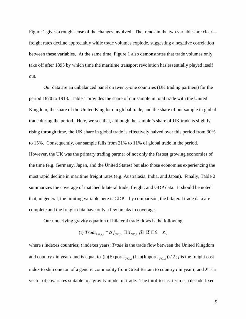
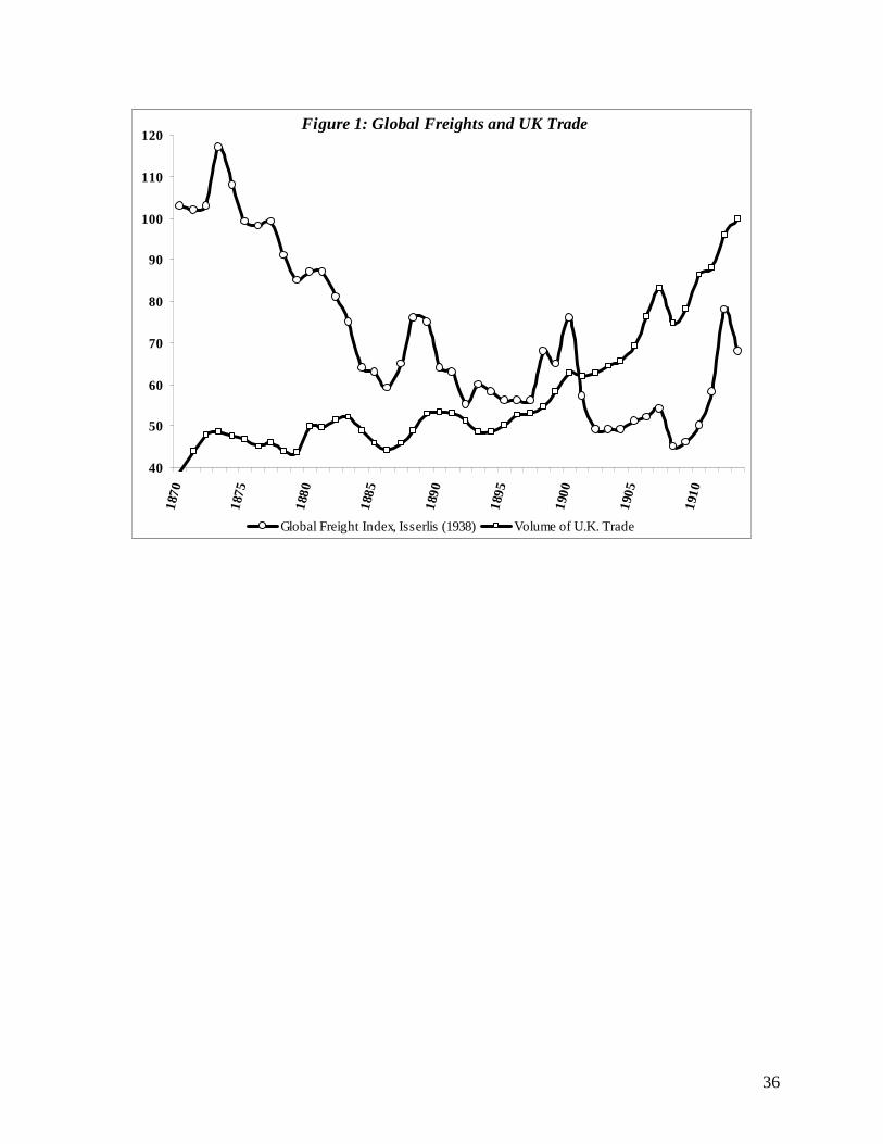
Figure 1 gives a rough sense of the changes involved. The trends in the two variables are clear—
freight rates decline appreciably while trade volumes explode, suggesting a negative correlation
between these variables. At the same time, Figure 1 also demonstrates that trade volumes only
take off after 1895 by which time the maritime transport revolution has essentially played itself
out.
Our data are an unbalanced panel on twenty-one countries (UK trading partners) for the
period 1870 to 1913. Table 1 provides the share of our sample in total trade with the United
Kingdom, the share of the United Kingdom in global trade, and the share of our sample in global
trade during the period. Here, we see that, although the sample’s share of UK trade is slightly
rising through time, the UK share in global trade is effectively halved over this period from 30%
to 15%. Consequently, our sample falls from 21% to 11% of global trade in the period.
However, the UK was the primary trading partner of not only the fastest growing economies of
the time (e.g. Germany, Japan, and the United States) but also those economies experiencing the
most rapid decline in maritime freight rates (e.g. Australasia, India, and Japan). Finally, Table 2
summarizes the coverage of matched bilateral trade, freight, and GDP data. It should be noted
that, in general, the limiting variable here is GDP—by comparison, the bilateral trade data are
complete and the freight data have only a few breaks in coverage.
Our underlying gravity equation of bilateral trade flows is the following:
, , , , , , ,(1) UK i t UK i t UK i t t i i tTrade f Xα β δ θ ε= + + + +
where i indexes countries; t indexes years; Trade is the trade flow between the United Kingdom
and country i in year t and is equal to UK,i,t UK,i,t(ln(Exports ) ln(Imports )) / 2+ ; f is the freight cost
index to ship one ton of a generic commodity from Great Britain to country i in year t; and X is a
vector of covariates suitable to a gravity model of trade. The third-to-last term is a decade fixed

10
effect to control for secular changes in world GDP and other variables. The second-to-last term
is a country fixed effect to control for time-invariant multilateral barriers and/or price effects
which capture the average trade barrier facing countries (Anderson and van Wincoop, 2003).1 In
addition, these country fixed-effects absorb all other time-invariant factors which affect
international trade volumes including the geographical distance between trading partners,
membership in the British Empire, use of the English language, and other cultural factors.
The freight cost index used in (1) constitutes a primary contribution of this paper and
varies across countries and over time. All extant freight cost indices are either commodity- and
city-specific as in Mohammed and Williamson (2004) or invariant across countries as in Isserlis
(1938). We use information on 5247 shipments of 40 different commodities during the period
1870 to 1913 between the United Kingdom and our sample of 21 countries. These shipping data
were collected from a number of sources, detailed in Appendix I, while Appendix II delves in
greater length into the composition of the underlying freight rates series in terms of country,
commodity, and route coverage.
We model the freight index as , , , ( )UK i t UK if f t= where , ( ),UK if t i = 1,...,21 are country-
specific freight rate indices, each of which is estimated as part of the function:
, , , , , , , ,(2) ln ( )UK i s t i UK i i s UK i s tF f t uδ φ= + + + .
1 Appendix III considers other formulations of the gravity equation which address the
identification problem highlighted by Baldwin and Taglioni (2006). Specifically, they
incorporate country-specific time dummies. The results presented in the following section
remain qualitatively unaltered by the addition of country-specific decade dummies. In the body
of this paper, we present results with country fixed-effects and decade fixed-effects, but without
their interaction as these diminish the identifying power of the freight variable.
11
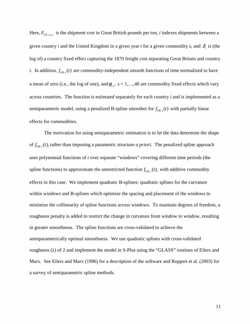
Here, , , ,UK i s tF is the shipment cost in Great British pounds per ton, i indexes shipments between a
given country i and the United Kingdom in a given year t for a given commodity s, and iδ is (the
log of) a country fixed effect capturing the 1870 freight cost separating Great Britain and country
i. In addition, , ( )UK if t are commodity-independent smooth functions of time normalized to have
a mean of zero (i.e., the log of one), and, ,i sφ s = 1,…,40 are commodity fixed effects which vary
across countries. The function is estimated separately for each country i and is implemented as a
semiparametric model, using a penalized B-spline smoother for , ( )UK if t with partially linear
effects for commodities.
The motivation for using semiparametric estimation is to let the data determine the shape
of , ( ),UK if t rather than imposing a parametric structure a priori. The penalized spline approach
uses polynomial functions of t over separate “windows” covering different time periods (the
spline functions) to approximate the unrestricted function , ( ),UK if t with additive commodity
effects in this case. We implement quadratic B-splines: quadratic splines for the curvature
within windows and B-splines which optimize the spacing and placement of the windows to
minimize the collinearity of spline functions across windows. To maintain degrees of freedom, a
roughness penalty is added to restrict the change in curvature from window to window, resulting
in greater smoothness. The spline functions are cross-validated to achieve the
semiparametrically optimal smoothness. We use quadratic splines with cross-validated
roughness (λ) of 2 and implement the model in S-Plus using the “GLASS” routines of Eilers and
Marx. See Eilers and Marx (1996) for a description of the software and Ruppert et al. (2003) for
a survey of semiparametric spline methods.

12
There are three crucial assumptions embodied in our semiparametric estimation of freight
rate indices. First, we use country-specific, but time-invariant coefficients for the 40 different
commodities we observe in our sample. This implies that, in any given country, the prices for
shipping different commodities must be related by the same proportionate differences over the
entire period. Historically, this restriction may be justified by considering freight rates in the
North Atlantic, the most heavily traveled route. In 1870, grain could be transported between
Britain and the US at 30% of the cost per ton of cotton. Likewise, wheat could be transported at
20% of the cost. In 1913, the respective figures were 25% and 16%. Given that the overall
maritime freight rate index for this route fell by 45% between 1870 and 1913, the above changes
on the order of 5% are relatively small and likely of second-order importance. Second, the
penalized splines employ a small number of windows and a roughness penalty that delivers a
freight index which varies smoothly over time and does not allow for discrete jumps or falls in
freight costs. Both of these assumptions are imposed to deliver a tractable empirical model. If
either is relaxed, the resulting model has too many parameters to feasibly estimate.
Finally, since we are interested in the total volume of trade between country i and the
United Kingdom, i.e. imports plus exports, we estimate equation (2) using information on both
UK-bound and -originated freight rates. In this sense, the , ( )UK if t term can be thought of as the
commodity-independent average freight rate separating country i and the United Kingdom. This
method also avoids the problem that indices derived from freight rates in only one direction, e.g.
from the United States to the United Kingdom, are likely to be biased as back-haulage rates were
vitally affected by both outward-bound rates and the composition of trade between two countries.
Figure 2 gives the reader a rough sense of this approach by plotting all available per-ton
freight rates between the United States and the United Kingdom against our UK-US freight rate

13
index as estimated from equation (2). The results are reassuring as the main trends in the data
seem to be captured well. From 1870 to 1913, the index registers a 45% decline for the UK-US
as compared to the 34% decline reported in the standard source on freight rates for this period
(Isserlis, 1939). Again, we emphasize that this Isserlis series which was used by Estevadeordal
et al. (2003) among others is simply a chained, unweighted average of a large number of
disparate freight rate series with no controls for commodities or routes and is, thus, country-
invariant. We believe that explicitly modeling the structure of freight rates as in equation (2) as
well as allowing for cross-country differences in the evolution of freight rates is an important
step in the right direction.
Next, we incorporate the country-specific freight indices into the vector of covariates X of
equation (1) which includes standard gravity model variables: GDP, income similarity, average
tariff intensities and exchange rate volatility for the United Kingdom and the twenty-one sample
countries, plus an indicator for gold standard adherence by each trading partner.2 The data are
described and summarized in Table 3 while the sources are detailed in Appendix IV.
IV. Results
In what follows, we take a very agnostic approach to our estimation strategy. Since our
main task is in exploring the co-movement of maritime freight rates and global trade flows, we
have avoided at the moment the issue of developing a fully specified, micro-founded model of
international trade in which to ground our gravity equation. And as our concern does not lie in
utilizing the gravity equation as a means of testing the empirical validity of any particular
2 The United Kingdom was, of course, on the gold standard for the entire period from 1870 to
1913.

14
modeling approach (Feenstra et al. 2001; Evenett and Keller, 2002), we are then on safe ground
in making the following assumptions about the gravity equation: simply, that the level of
bilateral trade flows should be increasing in economic size and in income similarity. Notably,
accounting for time-invariant unobservables with country fixed effects “knocks out” classic
gravity variables such as distance.3
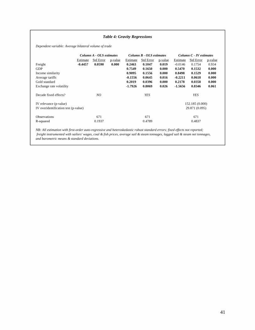
Our first exercise is to simply run a very naïve regression of bilateral trade flows on
nothing more than a constant and our measure of bilateral freight rates. These results are
reported in column A of Table 4 and strongly confirm the traditional story of the role of the
maritime transport revolution in the nineteenth century global trade boom. The estimated
elasticity between the two variables is precise, large, and negative. A ten percent drop in freight
rates is associated with an increase in trade volumes of over four percent. Thus, the drop in
average freight rates between 1870-75 and 1908-13 is predicted to explain approximately fifty
percent of the change in U.K. trade volumes in the same period.
Of course, this is the wrong exercise for evaluating the relationship of interest in light of
the considerable body of research into gravity models of international trade flows. Thus, we
include standard gravity variables—GDP, income similarity, tariff intensity, the gold standard,
and nominal exchange rate volatility. GDP is defined as(log log )UK iGDP GDP+ while income
similarity is measured by log UK i
UK i UK i
GDP GDP
GDP GDP GDP GDP
× + +
. Tariff intensities are defined as
3 The use of country fixed effects also allows us to avoid the issue of making the freight rate
indices—which are estimated at the country level as mean-zero series—strictly comparable
across countries. Thus, identification of the effects of the maritime transport revolution will
instead solely come from the proportionate changes in trade and freight rates within countries.

15
,
Tariff revenuelog average
ImportsUK i
. We note that we lack country-pair specific information on
tariff barriers—that is, these measures capture the general level of protection afforded in the UK
and US markets, for example, but not the protection afforded against British goods in US
markets and vice versa. At the same time, these same measures have been shown to correlate in
sensible ways with such things as trade costs and flows (Jacks et al., 2006). Likewise, adherence
to fixed exchange rate regimes as a stimulus to bilateral trade has a fairly long provenance in the
literature (Rose, 2000) and especially in the context of the gold standard of the late nineteenth
century (López-Córdova and Meissner, 2003).
When we incorporate these variables, the picture changes radically. Column B of Table 4
reports the results of OLS estimation of the gravity equation. Conforming to our priors, we find
significant positive coefficients for GDP, income similarity, and the gold standard as well as
significant negative coefficients for average tariffs and exchange rate volatility. But by far, the
most striking result is that for the freight rate term. Whereas in Column A the relationship was
decidedly negative, here in column B the relationship is decidedly positive.4
What explains this divergence from the previous results and, more pointedly, the
traditional narrative of the nineteenth century? In this take, the relationship should be a negative
one as lower freight rates drive down the costs of international trade and, thus, stimulate an
increase in observed trade volumes. Such a result would be consistent with the findings of Baier
and Bergstrand (2001) in company with Estevadoreal et al. (2003), both of which invoke the
exogeneity of transportation costs in explaining the growth of world trade.
4 We note that this finding is not affected by the inclusion of time-variant fixed effects or other
freight indices. Appendix III reports the results of this sensitivity analysis.
16
We believe there is another explanation, namely that freight rates are not exogenous.
One of our key arguments is that there has been insufficient appreciation of the following facts:
1.) freight rates are nothing but the prices for transport services and as such are a function of the
supply of shipping and the volume of trade demanded; and 2.) the volume of trade is a function
of traded prices and the quantity of goods shipped. In other words, the two variables—trade
volumes and freight rates—are simultaneously determined.
In the next battery of regressions, we address this endogeneity by instrumenting for the
freight price indices ( )if t using a vector of instruments which includes the log of Norwegian
sailors’ wages, log of the prices of coal and fish, the log of the average tonnages of sail and
steamships registered in the United Kingdom, the log of the (once- and twice-lagged) net
tonnage of British sail and steamships, and the annual mean and variance of barometric pressures
in four quadrants around the United Kingdom (the Baltic and North Seas, the Mediterranean Sea,
and the North and South Atlantic). The basic idea here is to isolate the supply curve of shipping
services from changes in demand, and we can motivate out instruments as follows.
Wage bills constituted a significant portion of variable costs in shipping. However, using
British sailors’ wages would be inappropriate as these wages are likely correlated with the
British business cycle and, thus, import demand. We exploit a different source of exogenous
variation in sailors’ wages. Hiring Norwegian sailors was a common occurrence on merchant
ships of all flags throughout this period, so their wages are likely to be highly correlated with,
but not wholly dependent upon those prevailing in the British shipping industry as their labor
was, in effect, an internationally traded commodity (Grytten, 2005). Such wages are likely to be
a suitable instrument in that they should be correlated with freight rates but not with the error
term, i.e. they only affect trade volumes indirectly through freights. Likewise, coal was a major

17
input to the production of shipping services during the period, but the share of coal consumed by
the industry was relatively small with 1.3% and 1.2% of British coal output in 1869 and 1903,
respectively, being allocated to coaling stations which acted as the depositories for coal
consumed in maritime transport (Griffin, 1977).
The measures of fish prices and route-specific barometric pressures are intended to
capture climatic effects on the supply of shipping with the idea being that inclement weather
over a year should have an adverse effect on the level of freight rates. The average tonnage of
sail and steamships is intended to capture exogenous technological change in the shipping
industry. As refinements in steamship technology were adopted and the physical size of
steamships ballooned, the cost advantages of steam versus sail mounted and shifted out the
supply curve of shipping over the long-run. And as these average tonnages enter logarithmically,
these variables capture the ratio of the average steamship size to that of the average sail ship
which should not be contemporaneously correlated with prevailing freight rates. We have
measures of the stock of net tonnage in the sail and steam fleets of the United Kingdom at our
disposal. Capacity constraints should vitally affect freight rates. However, we only include
lagged values of these measures to avoid the simultaneity between what is the quantity supplied
(net tonnages) and price (freight rates) of shipping service. Finally, as freight rates are
dependent on the distance separating ports, we also interact all instruments with the distance
between country i’s chief port and London.
The use of instrumental variables may also correct for the endogeneity of freight rates
due to correlated missing variables. One such correlated missing variable is unobserved declines
in overland shipping costs within the partner countries, particularly the introduction and
extension of railroad networks. These costs bear on the alternative to maritime trade with the

18
United Kingdom, i.e., domestic trade. Our instruments are based on the weather, sail and steam
tonnages, sailors’ wages, fish prices and UK coal prices. Noting that coal is a relatively small
input to rail and other overland transport, all these instruments are plausibly uncorrelated with
overland freight costs. Consequently, our IV regressions can be thought of as dealing with
unobserved declines in overland freight costs.
The instruments we chose are reasonably correlated with our endogenous variables of
interest. In our baseline model, the R-squared of the first stage regression is 0.84, and the Shea
partial R-squared of excluded instruments is 0.21. In addition, these instruments are plausibly
exogenous: the test of overidentifying restrictions has a p-value of about 10%. The results of the
instrumental-variables exercise are reported in Column C of Table 4. The coefficient on freight
is now small, negative, and statistically indistinguishable from zero.5 Taking together, these
results suggest that we are correctly identifying the relationship between trade flows and freight
rates, namely that freight rates are partially determined by the volume of trade—or more broadly,
the degree of economic integration—demanded by nations. However, once these demand-
induced changes in freight rates are accounted for, freight rates seem to have little independent
bearing on the volume of trade as the coefficient on freight in Column C is effectively zero.
5 The z-test statistic on an exclusion restriction for a constructed, endogenous regressor is
asymptotically normally distributed. This is because the semiparametric estimate of our
constructed regressor is consistent under the model and because the constructed regressor is not
in the model under the null hypothesis. See Section 6.2 of Newey and McFadden (1994).
19
V. What Drove the Nineteenth Century Trade Boom?
In the preceding, we have presented the evidence on the relationship linking trade flows
and freight rates with the view of determining the sources of globalization, both in the past and
the present. As of yet, we have reached a seemingly negative conclusion: there is little evidence
suggesting that the maritime transport revolution was a primary driver of the late nineteenth
century global trade boom.6
If this conclusion is warranted, it raises the issue of what might be the other, true drivers.
In order to provide an answer, we turn to the work of Baier and Bergstrand (2001). There, they
argue that a general equilibrium gravity model of international trade implies that roughly two-
thirds of the growth of world trade post-1950 can be explained by income growth, one-fourth by
tariff reductions, and less than one-tenth by transport-cost reductions while virtually none of the
growth in trade can be explained by income convergence. In the following, we suggest implicitly
6 At the same time, there is a voluminous body of work on commodity price convergence
throughout the nineteenth century (O’Rourke and Williamson, 1994, and Jacks, 2005). In the
most influential contribution to this literature, O’Rourke and Williamson write that the
“impressive increase in commodity market integration in the Atlantic economy [of] the late
nineteenth century” was a consequence of “sharply declining transport costs” (1999, p. 33).
However, O’Rourke and Williamson (1999) are quick to point out that a host of other factors
could also be responsible for the dramatic boom in international trade during the period, chief
among them being increases in GDP and import demand.

20
invoking their underlying model of world trade and explicitly following their lead by estimating
the following equation7:
, 1 , 2
3
4
(3) ( ) log( ) (log log )
log( )
Tariff revenue log average
Imports
UK i UK i UK i
UK i
UK i UK i
UK
Trade Freight GDP GDP
GDP GDP
GDP GDP GDP GDP
β β
β
β
∆ = ∆ + ∆ +
+ ∆ ×+ +
+ ∆
,
5 6 ( ) ,
i
i UKi iGold Exchange rate volatilityβ β ε
+ ∆ + ∆ +
where ∆ denotes the change in a variable over a ten year period. What we are trying to achieve
here is comparability of results for the nineteenth and twentieth centuries as well as provide
another test of the independent role of freight rates in determining the volume of trade.
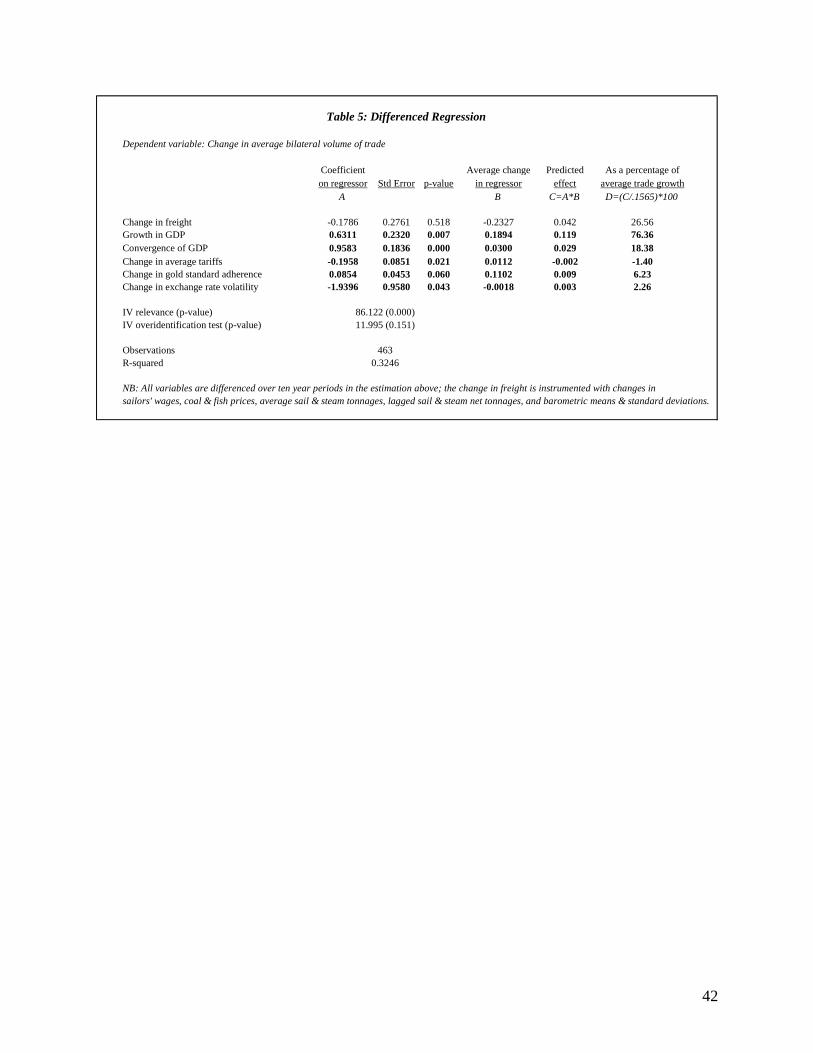
The results of this exercise are presented in Table 5. Once again, the instrumented freight
variable fails to register—whether by sign or significance—in a manner consistent with
prevailing narratives of a transport-led global trade boom in the late nineteenth century.
However, the variables capturing changes in income growth, convergence, tariffs, gold standard
adherence, and exchange rate volatility are all highly statistically significant and signed
consistently with the results of Table 4.
Coupled with the sample means of the variables reported in Table 3, the point estimates
allow us to decompose the relative contribution of these variables. Clearly, the overwhelming
majority (>75%) of the change in trade volumes is explained by the growth of economies in this
period—a result which compares well with the 65% figure from O’Rourke and Williamson
(2002) for 1500 to 1800, the 67% figure from Baier and Bergstrad (2001) for 1958 to 1988, and
7 We have slightly augment the model of Baier and Bergstrand by incorporating terms for secular
changes in the gold standard and exchange rate volatility.

21
the 76% figure from Whalley and Xin (2007) for 1975 to 2004. Unlike Baier and Bergstrand
(2001), we are also able to associate income convergence with the growth of trade volumes as
this variable explains 18% of the variation of the dependent variable—a result which might be
explainable by the greater convergence forces in effect for the pre-World War I era (O’Rourke et
al., 1996). Finally, we find significant but relatively mild trade-enhancing effects for the gold
standard (+6.23%) and the decline in nominal exchange rate volatility (+2.26%) as well as trade-
diminishing effects for average tariffs (-1.40%).8
VI. Conclusion
As seen above, this paper has established two important facets of global trade which are
likely to be just as applicable to the post-WWII trade boom as the pre-WWI one. First, greater
care must be taken in future work considering the relationship between transportation costs and
trade volumes as they are simultaneously determined. Second, and more fundamentally, once
this endogeneity is dealt with in appropriate fashion there is potentially little room for maritime
transport revolutions to be the primary drivers of the two global trade booms of the nineteenth
and twentieth centuries. Rather, the most powerful forces driving the boom were those of
income growth and convergence—a finding established here and congruent with a mounting
8 Partially controlling for the potential endogeneity of GDP by netting out the balance of trade
(i.e., X+M in the GDP equation) leaves the results largely unchanged. And since most of the
countries in our sample ran large, persistent trade surpluses with the United Kingdom, this direct
(accounting) effect of trade on GDP probably dominates any second order effects on, for
instance, scale and efficiency.

22
body of research on the sources of trade growth spanning not only the late twentieth century but
all the way back to the beginning of the global trading system in 1500.
In balance, these results allow for a potential revision of the first wave of globalization—
one in which the maritime transport revolution is substituted by the general progression and
convergence of incomes and in which freight rates are driven by the “demand” for globalization.
In this view of the world, the key innovations in the shipping industry, e.g. iron hulls and the
screw propeller, were induced technological responses to the heightened trading potential of the
period (see Peet, 1969, for an earlier statement of this view). Analogously, the movement
towards containerization of the world mercantile fleet was strongly conditioned upon agents’
expectations of commercial policy in light of attempts to re-establish the pre-war international
economic order (Levinson, 2006). In short, exploring this potential causal connection between
technological innovation and the diplomatic and political environment surrounding world trade
remains an important task for future research.
Another possibility that our results suggest is that focusing solely on the secular decline
in freight rates across the nineteenth century may be misleading. Aggregate trade costs of the
countries in our sample fell on average by around 15% from 1870 to 1913 (Jacks et al., 2006).
How can such a finding be reconciled with the very well-documented decline in maritime freight
rates in the period? First, transportation costs are only one input into trade costs, as emphasized
by Anderson and van Wincoop (2004). A broader look at the factors contributing to declines in
trade costs should include overall shipping and freight rates, the rise of the classical gold
standard and the financial stability it implied, and improved communication technology. There
were also countervailing effects of tariffs. These rose on average by 50 percent between 1870
and 1913 (Williamson, 2006). In addition, new non-tariff barriers were erected (Saul, 1967).

23
At the same time, the results also warrant some caution. First, it could be argued that the
United Kingdom might well be a peculiar unit of observation. Given the heavy share of raw
materials and especially food stuffs in its imports, it may have found itself on an inelastic section
of its demand curve, i.e. the level of freight rates would not affect the decisions of importers.
However, given that separate gravity equations estimated for imports and exports (not reported)
yield symmetric results, it seems unlikely that this is generating our findings.
Second, more work needs to be done in documenting and testing the complementary
decline in overland freight rates during this period. In some instances, the introduction of the
railroad and the telegraph led to declines in transportation costs on the order of 90% (but this
number was subject to wide variation). This point can be seen in the example of the grain trade
between the UK and US after 1850. Much of the decrease in the price differential between the
UK and US markets came through a narrowing of price gaps separating the Midwest and the East
coast of the US (O’Rourke and Williamson, 1994). The ever-expanding networks of railroads
and telegraphs lowered transportation costs between the Midwest and the Atlantic ports at a
faster rate than the observed decline in maritime freight rates. Jacks (2005) documents a similar
pattern based on commodity price data for a large set of countries which shows much faster
within country integration than cross-border integration over the period from 1800 to 1913.
Thus, the differential decline in overland and maritime freight rates across countries might tell a
different story, and we encourage others to follow our lead. Yet as we have argued before, to the
extent that within-country freight costs are uncorrelated with the supply-side instruments we use,
our instrumental variables strategy corrects for such excluded changes in overland transportation
costs.
24
Finally, recent research has suggested that the period prior to 1870 might have, in fact,
been the “big bang” period for the maritime transport revolution. Again, Jacks (2006)
documents a decline in the price gap for wheat separating London and New York City from 1830
to 1913 of 88%. Yet this decline was highly concentrated—of that 88%, the period from 1830 to
1870 witnessed a 74% decline with the remaining 14% decline being contributed in the period
from 1870 to 1913. It stands to reason that if maritime transport revolutions matter we should
also be looking at the early nineteenth century for clues. Unfortunately, systematic freight,
output, and trade data are all lacking for this earlier period. But there are some fragments at our
disposal: real US trade with 10 European countries and Canada grew 449% between 1870 and
1913 but only 412% between 1830 and 1870 (Treasury Department, 1893). Of course, one needs
to condition on standard gravity variables as argued above, but prima facie this suggests that if
anything the response of trade in the face of an even steeper decline in freight rates from 1830 to
1870 was more muted. Only ongoing work by economic historians piecing together the trade
history of the early nineteenth century will allow us to test this hypothesis directly.
25
Appendix I: Sources of Freight Rates
The richest single source for nineteenth century freight rates is Angier (1920). This provided
3049 of the 7923 observations in the global freight rate dataset available from the authors. Of
these 7923 observations, 5247 comprise either UK-destined or –originated freights and were
used in this paper. The following comprises the full list of sources.
Andrews, F. (1907), “Ocean Freight Rates and the Conditions Affecting Them.” USDA Bureau
of Statistics Bulletin no. 67. Washington: GPO.
Angier, E.A.V. (1920), Fifty Years' Freights 1869-1919, London: Fairplay.
Berry, T.S. (1984), Early California. Richmond: The Bostwick Press.
Board of Trade (1903), British and Foreign Trade and Industrial Conditions. London: Eyre and
Spottiswoode.
Brentano, L. (1911), Die Deutschen Getreidezölle. Stuttgart.
California State Agricultural Society (1891-1896), 1890-5 Transactions. Sacramento.
Daish, J.B. (1918), The Atlantic Port Differentials. Washington: W.H. Lowdermilk & Co.
Great Britain (1905), Parliamentary Papers.
Harley, C.K. (1988), “Ocean Freight Rates and Productivity, 1740-1913.” Journal of Economic
History 48(4), 851-876.
Harley, C.K. (1989), “Coal Exports and British Shipping, 1850-1913.” Explorations in Economic
History 26(3), 311-338.
Harley, C.K. (1990), “North Atlantic Shipping in the Late 19th Century: Freight Rates and the
Interrelationship of Cargoes.” In Shipping and Trade, 1750-1950, Fischer and Nordvik
(Ed.s). Pontefract: Lofthouse Publications, pp. 147-172.

26
Hobson, C.K. (1914), The Export of Capital. London: Constable & Co.
Jevons, H.S. (1909), Foreign Trade in Coal. London: P.S. King & Son.
Jevons, H.S. (1969), The British Coal Trade. New York: Augustus M. Kelley.
Johnson, E.R. (1906), Ocean and Inland Water Transportation, New York: Appleton.
Kuczynski, R.R. (1902), “Freight-Rates on Argentine and North American Wheat.” Journal of
Political Economy 10(3), 333-360.
McCain, C.C. (1893), Report of Changes in Railway Transportation Rates on Freight Traffic
throughout the United States. Washington: CPO.
Mitchell's Maritime Register. Various years.
New York Maritime Register. Various years.
D.C. North, D.C. (1958), “Ocean Freight Rates and Economic Development 1750-1913.”
Journal of Economic History 18(4), 537-555.
Rubinow, I.M. (1908), “Russia's Wheat Trade.” USDA Bureau of Statistics Bulletin no. 65.
Washington: GPO.
Sundbaerg, G. (1908), Apercus Statistiques Internationaux. Stockholm: Imprimerie Royale.
Thomas, D.A. (1903), “The Growth and Direction of our Foreign Trade in Coal during
the Last Half Century.” Journal of the Royal Statistical Society 66(3), 439-533.
27
Appendix II: Composition of Freight Rates Of primary concern in constructing freight rate indices as above is the composition and, thus,
representativeness of the underlying series. Table A.1 details the dataset of individual freight
rate observations along three dimensions. The first column considers the frequency with which
countries are represented in the data. At the top of the list, we find that a very substantial
proportion of the freight rates are taken from the United States. This is probably not surprising
as the United States was the United Kingdom’s largest trading partner (and the two were the
largest trading partners in the world throughout the period). At the same time, one can see that
most countries are very well-represented, including a number (e.g. Australasia, Ceylon, and
India) which witnessed the most dramatic drops in freight rates in the period under consideration.
The second column considers the commodities for which the freight rates were contracted. The
number one commodity was coal which, of course, was a primary export of the United Kingdom
at the time. Of the remaining twenty commodities, only the “General” and “Provisions”
categories could be interpreted as capturing manufactured goods. Thus, the freight rate indices
should capture the maritime transport revolution reasonably well to the extent that it vitally
affected high-bulk, low-value commodities. Finally, the third column details the most prominent
country and commodity pairings.

28
By country: By commodity (top 21 only): By country & commodity (top 21 only):N % N % N %
United States 1627 30.76 Coal 2037 38.51 United States, grain 537 10.23Russia 794 15.01 Grain 770 14.56 Italy, coal 449 8.56India 518 9.79 Wheat 567 10.72 United States, wheat 251 4.78Italy 450 8.51 General 303 5.73 France, coal 247 4.71Argentina 317 5.99 Deals 213 4.03 United States, flour 2104.00France 247 4.67 Flour 210 3.97 Argentina, coal 188 3.58Spain 237 4.48 Provisions 149 2.82 Russia, wheat 188 3.58Germany 180 3.40 Cotton 139 2.63 Germany, coal 180 3.43Chile 120 2.27 Ore 114 2.16 Russia, grain 179 3.41Australasia 116 2.19 Rice 76 1.44 India, coal 167 3.18Ceylon 115 2.17 Sugar 63 1.19 Spain, coal 165 3.14Brazil 101 1.91 Beef 58 1.10 Russia, coal 157 2.99Sweden/Norway 91 1.72 Pork 58 1.10 United States, provisions 149 2.84Canada 86 1.63 Phosphate 57 1.08 India, general 143 2.73Philippines 71 1.34 Hemp 44 0.83 United States, cotton 1372.61Portugal 48 0.91 Nitrate 40 0.76 Russia, deals 136 2.59Denmark 42 0.79 Bacon 38 0.72 Ceylon, coal 101 1.92Dutch East Indies 41 0.78 Jute 38 0.72 Chile, coal 80 1.52Japan 39 0.74 Wood 36 0.68 Brazil, coal 78 1.49Uruguay 31 0.59 Oats 35 0.66 Sweden/Norway, coal 72 1.37Colombia 19 0.36 Mutton 32 0.60 Argentina, wheat 64 1.22
Table A.1: Composition of freight rate series

29
Appendix III: Sensitivity Analysis
The following tables present the results of some sensitivity analysis. The inclusion of decadal
country fixed effects (i.e., there are five separate fixed effects for each of the twenty-one sample
countries) in the second column of Table A.2 is intended to capture any remaining unexplained
variation coming from time-varying country attributes. The specification preserves the sign of
the freight variable while decreasing its magnitude and significance. This does little to change
our basic story. This specification also destroys most of the explanatory power of remaining
variables, but the GDP and GDP shares remain large and highly significant. Additionally, this
specification comes closest to addressing the identification problems highlighted in Baldwin and
Taglioni (2006). The results are much the same for the IV specification presented immediately
below.
Dependent variable: Average bilateral volume of trade
OLS with fixed effects:Estimate Std Error p-value Estimate Std Error p-value
Freight 0.2463 0.1047 0.019 0.0692 0.0674 0.305GDP 0.7549 0.1650 0.000 0.8308 0.1250 0.000Income similarity 0.9095 0.1556 0.000 0.7300 0.1973 0.000Average tariffs -0.1556 0.0645 0.016 -0.0306 0.0755 0.686Gold standard 0.2019 0.0396 0.000 0.0633 0.0447 0.157Exchange rate volatility -1.7926 0.8069 0.026 -0.1466 0.6822 0.830
ObservationsR-squared
IV with fixed effects:Estimate Std Error p-value Estimate Std Error p-value
Freight -0.0146 0.1754 0.934 0.0572 0.1546 0.712GDP 0.5470 0.1532 0.000 0.7357 0.1421 0.000Income similarity 0.8498 0.1529 0.000 0.5185 0.1984 0.009Average tariffs -0.2211 0.0618 0.000 -0.0812 0.0561 0.148Gold standard 0.2178 0.0358 0.000 0.1037 0.0304 0.001Exchange rate volatility -1.5656 0.8346 0.061 -0.0431 0.6535 0.947
IV relevance (p-value)IV overidentification test (p-value)
ObservationsR-squared
NB: All estimation with first-order auto-regressive and heteroskedastic robust standard errors; fixed effects not reported.
0.7801
6710.7800
Country and decade fixed effects
671
226.696 (0.000)45.324 (0.002)29.871 (0.095)
6710.4837
Table A.2: Regressions with time-varying country fixed effects
6710.4789
Country and decade fixed effects
152.185 (0.000)
Decadal country fixed effects
Decadal country fixed effects
30
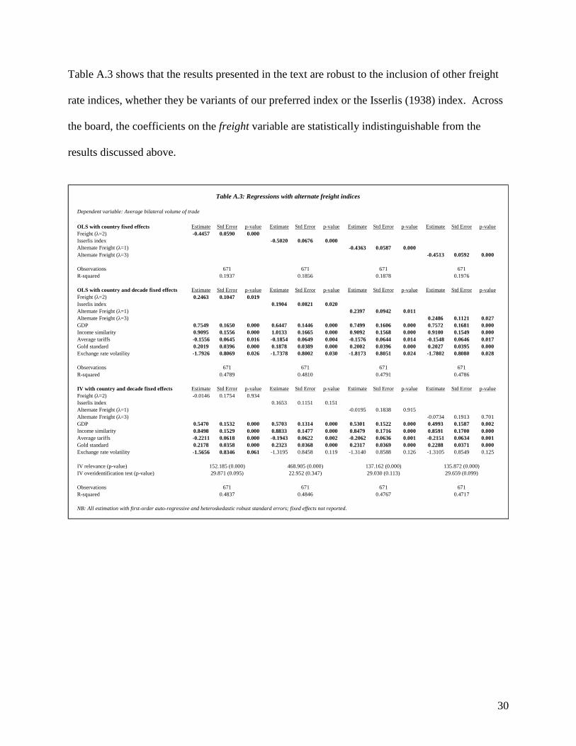
Table A.3 shows that the results presented in the text are robust to the inclusion of other freight
rate indices, whether they be variants of our preferred index or the Isserlis (1938) index. Across
the board, the coefficients on the freight variable are statistically indistinguishable from the
results discussed above.
Dependent variable: Average bilateral volume of trade
OLS with country fixed effects Estimate Std Error p-value Estimate Std Error p-value Estimate Std Error p-value Estimate Std Error p-valueFreight (λ=2) -0.4457 0.0590 0.000Isserlis index -0.5020 0.0676 0.000Alternate Freight (λ=1) -0.4363 0.0587 0.000Alternate Freight (λ=3) -0.4513 0.0592 0.000
ObservationsR-squared
OLS with country and decade fixed effects Estimate Std Error p-value Estimate Std Error p-value Estimate Std Error p-value Estimate Std Error p-valueFreight (λ=2) 0.2463 0.1047 0.019Isserlis index 0.1904 0.0821 0.020Alternate Freight (λ=1) 0.2397 0.0942 0.011Alternate Freight (λ=3) 0.2486 0.1121 0.027GDP 0.7549 0.1650 0.000 0.6447 0.1446 0.000 0.7499 0.1606 0.000 0.7572 0.1681 0.000Income similarity 0.9095 0.1556 0.000 1.0133 0.1665 0.000 0.9092 0.1568 0.000 0.9100 0.1549 0.000Average tariffs -0.1556 0.0645 0.016 -0.1854 0.0649 0.004 -0.1576 0.0644 0.014 -0.1548 0.0646 0.017Gold standard 0.2019 0.0396 0.000 0.1878 0.0389 0.000 0.2002 0.0396 0.000 0.2027 0.0395 0.000Exchange rate volatility -1.7926 0.8069 0.026 -1.7378 0.8002 0.030 -1.8173 0.8051 0.024 -1.7802 0.8080 0.028
ObservationsR-squared
IV with country and decade fixed effects Estimate Std Error p-value Estimate Std Error p-value Estimate Std Error p-value Estimate Std Error p-valueFreight (λ=2) -0.0146 0.1754 0.934Isserlis index 0.1653 0.1151 0.151Alternate Freight (λ=1) -0.0195 0.1838 0.915Alternate Freight (λ=3) -0.0734 0.1913 0.701GDP 0.5470 0.1532 0.000 0.5703 0.1314 0.000 0.5301 0.1522 0.000 0.4993 0.1587 0.002Income similarity 0.8498 0.1529 0.000 0.8833 0.1477 0.000 0.8479 0.1716 0.000 0.8591 0.1700 0.000Average tariffs -0.2211 0.0618 0.000 -0.1943 0.0622 0.002 -0.2062 0.0636 0.001 -0.2151 0.0634 0.001Gold standard 0.2178 0.0358 0.000 0.2323 0.0368 0.000 0.2317 0.0369 0.000 0.2288 0.0371 0.000Exchange rate volatility -1.5656 0.8346 0.061 -1.3195 0.8458 0.119 -1.3140 0.8588 0.126 -1.3105 0.8549 0.125
IV relevance (p-value)IV overidentification test (p-value)
ObservationsR-squared
NB: All estimation with first-order auto-regressive and heteroskedastic robust standard errors; fixed effects not reported.
152.185 (0.000) 468.905 (0.000)29.871 (0.095) 22.952 (0.347)
137.162 (0.000)29.030 (0.113)
135.872 (0.000)29.659 (0.099)
0.4837 0.4846 0.4767 0.4717671 671 671 671
6710.4789
Table A.3: Regressions with alternate freight indices
671 671671 671
671
0.1937 0.1856 0.1878 0.1976
6710.4810 0.4791 0.4786
671
31
Appendix IV: Sources of Gravity Variables
Coal export prices: Mitchell, B.R. (1994), British Historical Statistics. New York: Cambridge
University Press.
Exchange rates: Global Financial Database.
Fish prices: Urquhart, M.C. and K.A.H. Buckley (1965), Historical Statistics of Canada.
Toronto: MacMillan Company.
GDP and U.S. GDP deflator: Maddison, A. (2005), The World Economy: Historical Statistics.
Paris: OECD.
Monetary standards: Meissner, C. (2005), “A New World Order: Explaining the Emergence of
the Classical Gold Standard.” Journal of International Economics 66(2), 385-406.
Norwegian sailors’ wages: Grytten, O. (2005), “Real Wages and Convergence in the 19th
Century Maritime Labour Market.” Norwegian School of Economics.
Sail and steamship tonnage: Mitchell, B.R. (1994), British Historical Statistics. New York:
Cambridge University Press.
Sea-level pressures in the East North Atlantic and Europe: Luterbacher, J., E. Xoplaki, R. Rickli,
D. Gyalistras, C. Schmutz and H. Wanner (2002), “Reconstruction of Sea Level Pressure
Fields over the Eastern North Atlantic and Europe back to 1500.” Climate Dynamics
18(3), 545-61.
Tariffs (ratio of customs revenue to value of imports): Clemens, M.A. and J.G. Williamson
(2004), “Why did the Tariff-Growth Correlation Change after 1950?” Journal of
Economic Growth 9(1), 5-46.
U.K. exports and imports: Statistical Abstract for the United Kingdom. London: various years.

32
Works Cited Anderson, James E. and Erik van Wincoop (2003), “Gravity with Gravitas: A Solution to the
Border Puzzle.” American Economic Review 93(1), 170-192.
Baier, Scott L. and Jeffrey H. Bergstrand (2001), “The Growth of World Trade: Tariffs,
Transport Costs, and Income Similarity.” Journal of International Economics 53(1), 1-
27.
Baldwin, Richard and Daria Taglioni (2006), “Gravity for Dummies and Dummies for Gravity
Equations.” NBER Working Paper 12516.
Bernanke, Ben (2006), “Global Economic Integration: What’s New and What’s Not?”
http://www.federalreserve.gov/boarddocs/speeches/2006/20060825/default.htm
Berthelon, Matias and Caroline Freund (2004), “On the Conservation of Distance in International
Trade.” World Bank Policy Research Working Paper 3293.
Bhagwati, Jagdish (2004), In Defense of Globalization. Oxford: Oxford University Press.
Cameron, Rondo and Larry Neal (2003), A Concise Economic History of the World. Oxford:
Oxford University Press.
Carrère, Celine and Maurice Schiff (2004), “On the Geography of Trade: Distance is Alive and
Well.” World Bank Policy Research Working Paper 3206.
Disdier, Anna-Celia and Keith Head (2008), “The Puzzling Persistence of the Distance Effect on
Bilateral Trade.” Review of Economics and Statistics 90(1), 37-48.
Eilers, Paul and Brian D. Marx (1996), “Flexible Smoothing with B-splines and Penalties.”
Statistical Science 11(2), 89-121.
Estevadeordal, Antoni, Brian Frantz, and Alan M. Taylor (2003), “The Rise and Fall of World
Trade, 1870-1939.” Quarterly Journal of Economics 118(2), 359-407.

33
Evenett, Simon J. and Wolfgang Keller (2002), “On Theories Explaining the Success of the
Gravity Equation.” Journal of Political Economy 110(2), 281-316.
Feenstra, Robert C., James R. Markusen, and Andrew K. Rose (2001), “Using the Gravity
Equation to Differentiate among Alternative Theories of Trade.” Canadian Journal of
Economics 34(3), 430-447.
Griffin, Alan R. (1977), The British Coalmining Industry. Stoke-on-Trent: Wood Mitchell.
Grytten, O. (2005), “Real Wages and Convergence in the 19th Century Maritime Labour
Market.” Norwegian School of Economics.
Hummels, David (1999), “Have International Transportation Costs Declined?” Purdue
University.
Hummels, David (2001), “Toward a Geography of Trade Costs.” Purdue University.
Irwin, Doug A. (1995), “The GATT in Historical Perspective.” American Economic Review
85(2), 323-328.
Isserlis, L. (1938), “Tramp Shipping Cargoes and Freight.” Journal of the Royal Statistical
Society 101(1), 53-134.
Jacks, David S. (2005), “Intra- and International Commodity Market Integration in the Atlantic
Economy, 1800-1913.” Explorations in Economic History 42(3), 381-413.
Jacks, David S. (2006), “What Drove 19th Century Commodity Market Integration?”
Explorations in Economic History 43(3), 383-412.
Jacks, David S., Chris M. Meissner, and Dennis Novy (2006), “Trade Costs in the First Wave of
Globalization.” NBER Working Paper 12602.
James, Harold (2001), The End of Globalization. Cambridge: Harvard University Press.
Krugman, Paul (1995), “Growing World Trade: Causes and Consequences.” Brookings Papers

34
on Economic Activity (1), 327-377.
Leamer, Edward .E. and James Levinsohn (1995), “International Trade Theory: The Evidence.”
In G.M. Grossman and K. Rogoff (Ed.s), Handbook of International Economics, vol. III.
New York: Elsevier.
Levinson, Marc (2006). The Box. Princeton: Princeton University Press.
López-Córdova, J. Ernesto and Chris M. Meissner (2003), “Exchange-Rate Regimes and
International Trade: Evidence from the Classical Gold Standard Era.” American
Economic Review 93(1), 344-353.
Lundgren, Nils-Gustav (1996), “Bulk Trade and Maritime Transport Costs: The Evolution of
Global Markets.” Resources Policy 22(1), 5-32.
Mohammed, Shah S. and Jeffrey G. Williamson (2004), “Freight Rates and Productivity Gains in
British Tramp Shipping 1869-1950.” Explorations in Economic History 41(2), 172-203.
Newey, Whitney K. & McFadden, Daniel (1994), “Large Sample Estimation and Hypothesis
Testing.” In R. F. Engle and D. McFadden (Ed.s), Handbook of Econometrics, vol. IV.
New York: Elsevier.
O’Rourke, Kevin H., Alan M. Taylor, and Jeffrey G. Williamson (1996), “Factor Price
Convergence in the Late Nineteenth Century.” International Economic Review 37(3),
499–530.
O’Rourke, Kevin H. and Jeffrey G. Williamson (1994), “Late Nineteenth-Century Anglo-
American Factor-Price Convergence: Were Heckscher and Ohlin Right?” Journal of
Economic History 54(4), 892-916.
O’Rourke, Kevin H. and Jeffrey G. Williamson (1999), Globalization and History. Cambridge:
MIT Press.

35
O’Rourke, Kevin H. and Jeffrey G. Williamson (2002), “After Columbus: Explaining Europe’s
Overseas Trade Boom, 1500-1800.” Journal of Economic History 62(2), 417-456.
Peet, Richard (1969), “The Spatial Expansion of Commercial Agriculture in the Nineteenth
Century: A Von Thünen Interpretation.” Economic Geography 45(2), 283-301.
Rose, Andrew K. (2000), “One Money, One Market: Estimating the Effect of Common
Currencies on Trade.” Economic Policy 30(1): 7–45.
Saul, S.B. (1967), Studies in British Overseas Trade, 1870-1914. Liverpool: Liverpool
University Press, 1967.
Taylor, Alan M. and Jeffrey G. Williamson (1997), “Convergence in the Age of Mass
Migration.” European Review of Economic History 2(1), 27-63.
Treasury Department (1893), Statistical Tables Exhibiting the Commerce of the United State
with European Countries from 1790 to 1890. Washington: GPO.
Wand, M.P. and R.J. Carroll (2003), Semiparametric Regression. Cambridge: Cambridge
University Press.
Whalley, John and Xian Xin (2007), “Regionalization, Changes in Home Bias, and the Growth
of World Trade.” NBER Working Paper 13023.
Williamson, Jeffrey G. (2006), “Explaining World Tariffs, 1870-1913: Stolper-Samuelson,
Strategic Tariffs, and State Revenues,” in H. Lindgren R. Findlay, H. Henriksson and
M. Lundhal, eds., Eli Heckscher, International Trade, and Economic History.
Cambridge: MIT Press, 199-228.
36
Figure 1: Global Freights and UK Trade
40
50
60
70
80
90
100
110
120
1870
1875
1880
1885
1890
1895
1900
1905
1910
Global Freight Index, Isserlis (1938) Volume of U.K. Trade

37
Sample to UK UK to global Sample to global trade ratio trade ratio trade ratio
1870-1875 0.7116 0.2969 0.21111875-1880 0.7264 0.2629 0.19091880-1885 0.7369 0.2310 0.17031885-1890 0.7456 0.2193 0.16351890-1895 0.7508 0.2098 0.15751895-1900 0.7607 0.2013 0.15321900-1905 0.7657 0.1940 0.14861905-1910 0.7539 0.1692 0.12761910-1913 0.7412 0.1514 0.1122
Sources: Estevadeordal et al. (2003); Statistical Abstract for the United Kingdom.
Table 1: Trade Ratios

38
Countries with a full panel of GDP and freight data from 1870:Brazil JapanCanada (ends 1907) Portugal Ceylon RussiaDutch East Indies SpainFrance United StatesGermany Uruguay (ends 1907)Italy
Countries with a full panel of GDP and freight data from 1884:Australasia IndiaDenmark Norway & Sweden
Countries with a full panel of GDP and freight data from 1900:Argentina ColombiaChile Philippines
NB: Australia and New Zealand do not enter as separate trade entities before 1887; likewise, Norway and Sweden do not enter seperately until 1891.
Table 2: Sample Countries and Coverage

39
Figure 2: Freight Rates and Freight Indices
Pence-per-ton freight rates for the U.K. and U.S. & the Semiparametric Index
0
100
200
300
400
500
600
700
800
900
1000
1870
1875
1880
1885
1890
1895
1900
1905
1910
Freight rates Semiparametric Index

40
Description: N Mean Stand Dev Minimum MaximumVolume of trade Average of bilateral imports (log of) plus exports (log of) 671 20.38 1.206 17.22 22.58Freight Semiparametric index of country-specific freight rates (log of) 671 4.28 0.368 3.11 5.19GDP Sum of UK and partner GDP (log of) 671 12.32 0.334 11.69 13.53Income similarity Product of UK- and partner-shares of combined GDP (log of) 671 -2.31 0.860 -4.71 -1.39Average tariffs Average of partner and UK tariffs (log of) 671 2.30 0.511 1.25 3.46Gold standard Indicator variable for partner adherence to gold standard 671 0.56 0.497 0.00 1.00Exchange rate volatility Standard deviation of change in logged nominal exchange rate 671 0.01 0.014 0.00 0.10
Growth of trade Decadal difference in Volume of trade 463 0.1565 0.3108 -0.9414 1.7904Change in freight Decadal difference in Freight 463 -0.2327 0.1814 -0.7567 0.4213Growth in GDP Decadal difference in GDP 463 0.1894 0.0532 0.0638 0.4133Convergence of GDP Decadal difference in Income similarity 463 0.0300 0.0939 -0.1863 0.5062Change in average tariffs Decadal difference in Average tariffs 463 0.0112 0.2444 -0.7258 0.8139Change in gold standard adherence Decadal difference in Gold standard 463 0.1102 0.4349 -1.0000 1.0000Change in exchange rate volatility Decadal difference in Exchange rate volatility 463 -0.0018 0.0167 -0.0771 0.0930
Table 3: Data Summary
`
41
Dependent variable: Average bilateral volume of trade
Estimate Std Error p-value Estimate Std Error p-value Estimate Std Error p-valueFreight -0.4457 0.0590 0.000 0.2463 0.1047 0.019 -0.0146 0.1754 0.934GDP 0.7549 0.1650 0.000 0.5470 0.1532 0.000Income similarity 0.9095 0.1556 0.000 0.8498 0.1529 0.000Average tariffs -0.1556 0.0645 0.016 -0.2211 0.0618 0.000Gold standard 0.2019 0.0396 0.000 0.2178 0.0358 0.000Exchange rate volatility -1.7926 0.8069 0.026 -1.5656 0.8346 0.061
Decade fixed effects? NO YES YES
IV relevance (p-value)IV overidentification test (p-value)
ObservationsR-squared
NB: All estimation with first-order auto-regressive and heteroskedastic robust standard errors; fixed effects not reported; freight instrumented with sailors' wages, coal & fish prices, average sail & steam tonnages, lagged sail & steam net tonnages,and barometric means & standard deviations.
Column A - OLS estimates Column B - OLS estimates
671
Column C - IV estimates
6710.4837
Table 4: Gravity Regressions
0.1937 0.4789671
152.185 (0.000)29.871 (0.095)
42
Dependent variable: Change in average bilateral volume of trade
Coefficient Average change Predicted As a percentage ofon regressor Std Error p-value in regressor effect average trade growth
A B C=A*B D=(C/.1565)*100
Change in freight -0.1786 0.2761 0.518 -0.2327 0.042 26.56Growth in GDP 0.6311 0.2320 0.007 0.1894 0.119 76.36Convergence of GDP 0.9583 0.1836 0.000 0.0300 0.029 18.38Change in average tariffs -0.1958 0.0851 0.021 0.0112 -0.002 -1.40Change in gold standard adherence 0.0854 0.0453 0.060 0.1102 0.009 6.23Change in exchange rate volatility -1.9396 0.9580 0.043 -0.0018 0.003 2.26
IV relevance (p-value)IV overidentification test (p-value)
ObservationsR-squared
NB: All variables are differenced over ten year periods in the estimation above; the change in freight is instrumented with changes in sailors' wages, coal & fish prices, average sail & steam tonnages, lagged sail & steam net tonnages, and barometric means & standard deviations.
0.3246
Table 5: Differenced Regression
463
86.122 (0.000)11.995 (0.151)