Globalization and the Gains from Variety

Christian Broda (FRBNY)

and

David E. Weinstein (Columbia University and NBER)*

January 2005

Abstract

Since the seminal work of Krugman (1979), product variety has played a central role in models of trade and growth. In spite of the general use of love-of-variety models, there has been no systematic study of how the import of new varieties has contributed to national welfare gains in the United States. In this paper we show that the unmeasured growth in product variety from US imports has been an important source of gains from trade over the last three decades (1972-2001). Using extremely disaggregated data, we show that the number of imported product varieties has increased by a factor of four. We also estimate the elasticities of substitution for each available category at the same level of aggregation, and describe their behavior across time and SITC industries. Using these estimates we develop an exact aggregate price index and find that the upward bias in the conventional import price index is approximately 1.2 percentage points per year. The magnitude of this bias suggests that the welfare gains from variety growth in imports alone are 2.6 percent of GDP.

*We would to thank Fernando Alvarez, Alan Deardorff, Robert Feenstra, Jonathan Eaton, Amartya Lahiri, Mary Amiti, and Kei-Mu Yi for excellent comments and suggestions. Rachel Polimeni provided us with outstanding research assistance. David Weinstein was at the Federal Reserve Bank of New York when most of this research was done. In addition, he would like to thank the Center for Japanese Economy and Business for research support. The views expressed here are those of the authors, and do not necessarily reflect the position of the Federal Reserve Bank of New York, the Federal Reserve System, or any other institution with which the authors are affiliated.

Globalization and the Gains from Variety

I) Introduction

It is striking that in the quarter-century since Krugman (1979) revolutionized

international trade theory by modeling how countries could gain from trade through the import of

new varieties, no one has structurally estimated the impact of increased variety on aggregate

welfare. As a result, our understanding of the importance of new trade theory for national

welfare rests on conjecture, calibration, and case studies. While Feenstra (1992), Klenow and

Rodriguez (1997), Bils and Klenow (2001), and Yi (2003) made important inroads into our

understanding of the role played by new varieties and differentiated trade, this paper represents

the first attempt to answer the question of how much increases in traded varieties matter for the

US. Analyzing the most disaggregated US import data available for the period between 1972 and

2001, we find that consumers have low elasticities of substitution across similar goods produced

in different countries. Moreover, we find that the four-fold increase in available global varieties

arising in the last 30 years has produced a large welfare gain for the United States. Increases in

imported varieties have raised US real income by about 2.6 percent or four to ten times more

than conventional estimates that do not take new varieties into effect. In short, our results

provide stunning confirmation of the importance of thinking about international trade within a

framework of differentiated goods.

The starting point for our analysis is the seminal work of Feenstra (1994). In this paper,

Feenstra develops a robust and easily implementable methodology for measuring the impact of

new varieties on an exact price index of a single imported good using only the data available in a

typical trade database. Unfortunately, his approach has two drawbacks that have prevented

researchers from adopting it more widely. First, it cannot be used to assess the value of the

introduction of completely new product categories. Second, Feenstra’s methodology tends to

generate a large number of elasticities that take on imaginary values, which are hard to interpret.

This paper solves both problems and demonstrates the relative ease with which the Feenstra sub-

indexes can be used to compute an aggregate price index.

To calculate an aggregate import price index, we first have to estimate a number of

parameters that are of wide interest. This constitutes our second contribution. In particular, we

2

estimate elasticities of substitution among goods at various levels of aggregation. At the lowest

level of aggregation available for trade data (7-digit for 1972-1988 and 10-digit for 1990-2001)

we estimate almost 30,000 elasticities. This enables us to directly test a number of important

stylized facts. For example, we directly demonstrate the validity of Rauch’s (1999) conjecture

that goods traded on organized exchanges are more substitutable than those that are not. We are

able to document that varieties appear to be closer substitutes in more disaggregate product

categories. We also find that the median elasticity of substitution has fallen over time indicating

that traded goods have become more differentiated. In sum, we develop the most comprehensive

examination of import elasticities of substitution that has ever been attempted.

We then use these estimated parameters to reconstruct the US import price index while

hewing very closely to theory. Starting with the constant elasticity of substitution utility function

which underlies the Spence-Dixit-Stiglitz (henceforth SDS) framework, we compute an exact

aggregate price index for the CES utility function that allows for changes in varieties. Since this

is the same assumption that is used in much of the new trade theory, economic geography, and

growth literatures (Helpman and Krugman (1985), Grossman and Helpman (1991), Fujita,

Krugman, and Venables (1999)), our estimates can be directly applied to these literatures. Our

results suggest that the impact of increased choice on the exact import price index is both

statistically and economically significant. Whereas previous authors have found small changes in

import prices and the terms of trade as a result of variety changes, our study finds that price

indices that do not take new and disappearing varieties into account seriously overestimate

import price increases. Over the last thirty years, if one adjusts for new varieties, import prices

have been falling 1.2 percentage points per year faster than one would surmise from official

statistics. In aggregate terms this means that the aggregate price index that takes variety changes

into account has fallen by 28.0 percent relative to the conventionally measured import price

index.

Finally, we are able to use this price decline to obtain an estimate of the gains from new

imported varieties under the same structural assumptions as Krugman (1980). This massive drop

in our correctly measured price of imports drives our estimate of the gains from globalization.

The 28 percent drop in import prices due to new varieties alone implies that increases in

imported varieties have raised US welfare by about 2.6%. We show that the stronger

assumptions that are commonly used in the macro literature (e.g., Feenstra (1992), Romer (1994)

3

and Klenow and Rodriguez (1997)) would lead to welfare gains from variety up to three times

larger. Moreover, even when we relax Krugman’s (1980) assumptions and allow for perfect

substitution with domestic varieties, we find that unmeasured gains from trade are close to our

estimates. In sum, our results show that, when measured correctly, increases in imported

varieties have had a large positive impact on US welfare.

II) Prior Work

What is a variety? Previous work has not answered this question with a unified voice. In

terms of theory, a variety is commonly defined as a brand produced by a firm, the total output of

a firm, the output of a country, or the output within an industry in a county. As a result of the

variety of definitions of variety, empirical papers are often not strictly comparable. For example,

econometric case studies typically define a variety as a product line produced by a firm; many

international trade papers define a variety as a disaggregated trade flow from a particular

country; and still others have defined a variety either as firm- or plant-level output. The choices

are often driven by data availability and the types of theories that the researchers are examining.

While we will make precise our definition of variety later, we want to emphasize that as we

discuss prior work, the definition of variety will vary across papers.

Several studies have attempted to measure the impact of new varieties on welfare for

individual goods and at the aggregate level. Hausman (1981) pioneered an approach to

estimating the gains from new varieties (product line) of an individual good using micro data. He

develops a closed-form solution to estimating linear and log-linear demands and calculates the

new product’s ‘virtual price’, the price that sets its demand to zero. Based on this estimate and on

the current price, he calculates the welfare change that results from the price drop of the new

product. The advantage of this approach is that by taking enormous care to model, for example,

the market for Apple Cinnamon Cheerios, one can obtain extremely precise estimates that can

take into account rich demand and supply interactions. However, the data requirements to

implement this approach for the tens of thousands of goods that compose an aggregate price

index are simply insurmountable. For this reason, it is not surprising that no one has attempted to

estimate aggregate gains from new products using this approach.

At the aggregate level, all existing studies rely on calibration or simulation exercises to

measure the effect of variety growth. These studies typically define a variety as the imports from

4

a given country or the imports from a given country in a particular industry. These studies

typically do not focus on how varieties affect prices but rather provide some interesting

calculations about potential welfare effects. Feenstra (1992) and Romer (1994), for example,

provide numerical exercises showing that the gains from new varieties from small tariff changes

can be substantial. Klenow and Rodriguez-Clare (1997) calibrate a model of the impact of trade

liberalization on Costa Rica and find only modest gains. They suggest that the low elasticity of

substitution and large import shares used in Romer (1994) account for the difference in welfare

gains. 1

These papers have provided an invaluable first step in understanding how to move from

theory to data, but they require a large number of restrictive simplifying assumptions in order to

obtain the estimates. For example, these papers use one or at most two elasticities of substitution

in order to value varieties. This creates three types of problems. The first arises from assuming

that all elasticities of substitution are the same for varieties of different goods. Since presumably

consumers care more about varieties of computers than crude oil, it is not clear that all increases

in imports correspond to the same gains from increased variety. The second problem arises from

assuming that the elasticity of substitution across goods equals that across varieties of a given

good. Presumably we care more about the different varieties of fruits than about varieties of

apples. The final and perhaps largest problem arises from assuming that all varieties enter into

the utility function with a common elasticity. When one is estimating a parameter that is

averaging together, say, the impact of an increase of Saudi Arabian oil prices on Mexican oil

imports and Japanese car imports, it is hard to interpret the meaning of the elasticity or have

intuition for its magnitude.

A different class of problem with calibration exercises stems from the choice of the

parameter values and the use of symmetric utility functions (e.g., Romer (1994) and Broda and

Weinstein (2004)). Parameter values, such as elasticities of substitution, are often chosen

arbitrarily or are estimated from one dataset and applied to another dataset. An important feature

of our study is that all parameters are estimated directly from the relevant data and not chosen in

order to obtain sensible values for some other stage of the analysis. Moreover, in the case of a

symmetric utility function, since all varieties are valued alike a count of the number of imported

1 Rutherford and Tarr (2002) simulate a growth model with intermediate input varieties that magnifies the effect of trade liberalization on welfare, and suggest that a 10% tariff cut can lead, in the long run, to welfare gains of roughly 10%.

5

varieties is sufficient to perform welfare calculations. This approach is only valid under the

extreme symmetry assumptions underlying the particular utility function used. Indeed, this paper

shows that the use of count data, rather than the changes in import volumes as suggested by

Feenstra (1994), can be highly misleading as a measure of variety growth if one allows for a

more general utility function.

The third problem is related to the way in which previous studies have estimated the

single elasticity of substitution. By far the simplest of these approaches is to follow the

pioneering work of Anderson (1979) and estimate the elasticity of substitution by regressing

bilateral trade flows on various control variables and a measure of trade costs. The coefficient on

trade costs is used as the elasticity of substitution among varieties. The major problem with this

approach is that one needs to make extreme identifying assumptions in order to ignore

simultaneity problems. Chief among these is the assumption that trade costs are completely

passed through to consumers. This assumption is almost surely inappropriate for the US and the

other large importers who together account for the majority of world trade. A second problematic

identifying assumption is that movements in trade costs are unaffected by movements in import

demand. Unfortunately, this assumption will be violated whenever per unit transport costs are a

function of import volumes, countries care about import responses when cutting bilateral tariffs,

or movements in non-tariff barriers are correlated with movements in tariffs. Since all of these

conditions are likely to be violated in reality, the estimated elasticities are problematic. Ignoring

the simultaneity problem would result in lower estimates of the elasticities of substitution.

Our paper proceeds as follows. In Section III we provide an overview of the basic

theoretical contributions on the literature of variety growth and the reasons behind the structure

we use in this paper. In Section IV we provide descriptive statistics on the growth in varieties in

US imports since 1972. Section V is devoted to the methodology used to compute an exact

aggregate price index and to estimate elasticities of substitution that correct for endogeneity bias,

measurement error, and that allow for changes in taste and quality parameters. Section VI

presents the main results of the paper. We present our conclusions in Section VII.

III) Theory: Why do varieties matter?

All studies that seek to quantify the potential gains from variety are forced to impose

some structure on how varieties might affect welfare. Theorists have proposed many ways of

6

modeling this (see, for example, Hotelling (1929), Lancaster (1975), Spence (1976) and Dixit

and Stiglitz (1977)), and the assumptions underlying these models are not innocuous. As

empirical researchers, we are forced to choose from a number of plausible theories. Our choice

of the Spence-Dixit-Stiglitz (SDS) framework is based on three criteria: prominence,

tractability, and empirical feasibility.

There is little question that in international trade, economic geography, and

macroeconomics, the SDS framework is the preferred way of specifying how consumers value

variety. A major reason for this stems from the tractability of the CES utility function and its

close cousin, the Cobb-Douglas. In addition to the work of Krugman, the Dornbush, Fisher,

Samuelson models and more recent work by Eaton and Kortum (2002) all use CES and Cobb-

Douglas functions. Hence, it is quite natural to use this preference structure as the basis of our

empirical work. At the very least, our work provides a useful benchmark for thinking about the

potential gains from imported varieties within this framework.

A second reason to base our work on the SDS framework is theoretical tractability. As

Helpman and Krugman [(1985) pp. 124-129] note, preference systems based on the Hotelling

and Lancaster models do not easily lend themselves to the creation of aggregate price indexes or

utility functions when there is more than one market in the economy. Since one of the main

objectives of this study is to build an aggregate price index, we need to use a theoretical structure

that will let us aggregate price changes across markets.

Finally, the CES satisfies another important characteristic – empirical feasibility. Demand

systems based on CES utility functions are relatively easy to estimate. This is of paramount

importance since we need to be able to aggregate estimates of the gains from variety in tens of

thousands of markets. Moreover, since we know next to nothing about demand and supply

conditions in virtually all of the markets we examine, it is simply not feasible to implement a

more complex supply and demand structure.2 Thus, although one would ideally like to control

for all of the complexities present in international markets, data and time limitations required to

perform a careful analysis of all of these markets makes this impossible in practice.

Given our structure for how we model the way in which consumers value variety, we

now need to be precise about what we mean by a variety. Our reliance on the Krugman (1980)

2 One property of the CES is that, by assumption, consumers care about varieties to some extent. In practice, this assumption does not bias our results because an increase in variety will have a trivial impact on prices and welfare if the estimated elasticity of substitution is large.

7

structure might suggest that we adopt a definition of variety that is based on firm-level exports.

Unfortunately there are a number of problems with taking this literal approach to the data. First,

by treating all imports from a given firm as a single variety one may understate the gains from

variety that occur when a firm starts exporting in more than one product line. Second, it is

difficult to obtain bilateral firm-level export data for more than a handful of countries. We

therefore opt to use the same definition of variety as in Feenstra (1994) – namely, a 7- or 10-digit

good produced in a particular country. To give a concrete example, a good constitutes a

particular product, e.g. red wine. A variety, however, constitutes the production of a particular

good in a particular country, just as in Armington (1969), e.g. French red wine.

Being clear about this distinction highlights an important difference between

monopolistic competition models and comparative advantage models that feature a continuum of

goods. Both models share the feature that output of tradables is perfectly specialized in

equilibrium. However, they differ in terms of how individual varieties are treated. In the

comparative advantage continuum of goods models, consumers are indifferent about where a

good is produced as long as the price does not vary. In other words, these models assume that

holding the good fixed, the elasticity of substitution among varieties is infinite. This is in sharp

contrast to the Krugman model that hypothesizes that all firms produce differentiated products

and hence the elasticity of substitution should be small.

Despite the sharp theoretical difference, our ability to do precise hypothesis testing is

limited. The point estimate for the elasticity of substitution will always be finite and thus we can

never formally accept the hypothesis that it is infinite. However, by examining the elasticities of

substitution at the 7- or 10-digit level, we can obtain a sense of the degree of substitutability

among varieties. If the elasticities of substitution tend to be high, say above 10 or 20, then this

suggests that the potential for gains from variety, a key theoretical result of the monopolistic

competition framework, are small. If they are low, then this suggests that even when we use the

most disaggregated trade data in existence, goods are highly differentiated by country. Of course,

we cannot rule out that if we had even more disaggregated data, we might find a higher estimate

of the elasticity of substitution. Yet even so, we do learn something about the world – at the 7- or

10-digit level of aggregation, it is reasonable to think of goods from different countries as far

from perfect substitutes. More importantly for our purposes, low elasticities of substitution

8

across varieties are a necessary condition for increases in the number of varieties to be a source

of potential gain.

Turning to welfare, the monopolistic competition model described in Krugman (1979 and

1980) suggests two clear channels for the gains from trade arising from variety growth. The first

is through reductions in trade costs. If trade costs fall, countries will gain through the import of

new varieties.3 The second is through growth of the foreign country. As the size of the foreign

country rises (which in the Krugman framework is equivalent to a rise in its labor force), it will

produce more varieties, and this will also be a source of gain for the home country. These gains

are in sharp contrast to the gains postulated by comparative advantage models. In these models,

all goods are consumed in equilibrium regardless of the level of trade costs or the size of the

foreign country. Hence, in comparative advantage models, all gains from reductions in trade

costs or increases in the size of a foreign country are achieved through conventional movements

in prices and not through changes in the number of goods. One of the distinguishing features of

the Krugman model is that a country may gain from trade even though there are no price changes

of existing goods.

In sum, although theorists have developed a number of models of variety, our choice of

the Dixit-Stiglitz structure stems from that model’s prominence, tractability, and empirical

implementability. Moreover, since this model can easily explain key stylized facts of how the

growth of foreign countries and the reduction of international barriers have contributed to an

increase in US imports of varieties, we believe it is a particularly appropriate structure to use in

order to obtain estimates of the gains from variety.

IV) Data: The Growth of Varieties

It is well known that trade has been growing faster than GDP for many decades. This

process, which is a part of what some term “globalization,” has had a profound impact on the

dependence of the US economy on foreign goods. Over the last thirty years, the share of imports

of goods in US GDP has more than doubled: rising from 4.8 percent in 1972 to 11.7 percent in

2001.4 The causes for this explosion in trade stem from a number of sources that have been

3 The basic Krugman model predicts that a change in tariffs within non-prohibitive values will not change the number of available varieties although consumers will gain from the falling prices of imported varieties. Romer (1994), however, presents a simple extension of this model to allow for fixed costs of accessing foreign markets so that the number of available varieties rises with a fall in tariffs. 4 Data are from the World Bank World Development Indicators unless stated otherwise.

9

explored in a vast literature. Most studies attribute the source of the rise to three interrelated

causes: reductions in trade costs, relaxations of capital controls (e.g. barriers to foreign direct

investment), and the relative growth of many East Asian and other economies outside of the

United States.

This rise in US imports has been accompanied by a rise in another phenomenon that has

received much less attention – a dramatic rise in imported varieties. Table 1 gives a preliminary

overview of the extent of this increase. Between 1972 and 1988, we rely on the Tariff System of

the United States (TSUSA) 7-digit data and in later years on the 10-digit Harmonized Tariff

System (HTS) data (Feenstra (1996) and Feenstra et al. (2002)). We define a good to be an 7- or

10- digit category, and, as mentioned in the previous section, a variety is defined as the import of

a particular good from a particular country.5 We do not report numbers for 1989 because the

unification of Germany means that data for that year are not comparable with later HTS data.6

Using our definition of varieties, Table 1 reports that in 1972 the US imported 74,667

varieties (i.e. 7731 goods from an average of 9.7 countries) and in 2001 there were 259,215

varieties (16390 goods from an average of 15.8 countries). Ultimately, we will want to make

comparisons across years, and to do that properly we will need to formally deal with a host of

issues relating to whether the data for two different years are truly comparable. For now, we put

these issues aside and focus on the crude measure of variety that we can glean from the sample

statistics.

The second column of Table 1 reports the number of goods for which imports exceeded

one dollar in a given year. There are two features of this column that are important to note here.

First, comparing the values for 1988 and 1990, there appears to be little difference in the number

of categories with positive imports in the TSUSA and HTS systems. Second there appears to be a

dramatic increase in the number of US import categories over the time periods. Combining the

increases over the periods 1972-1988 and 1990 to 2001, it appears that the number of good

categories almost doubled. This establishes the importance of thinking about real or apparent

new goods or categories when calculating changes in import structure and the price of imports.

5 This definition matters less than one might suppose for our later empirical work since we will estimate elasticities of substitution across varieties of a good and let the data tell us how important differences among varieties are. For the time being, however, we will leave aside the question of how substitutable goods produced in different countries are, and simply focus on the number of varieties. 6 All the countries in the former Soviet Union are aggregated together throughout our analysis.

10

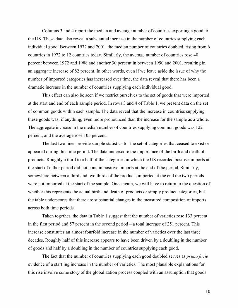
Columns 3 and 4 report the median and average number of countries exporting a good to

the US. These data also reveal a substantial increase in the number of countries supplying each

individual good. Between 1972 and 2001, the median number of countries doubled, rising from 6

countries in 1972 to 12 countries today. Similarly, the average number of countries rose 40

percent between 1972 and 1988 and another 30 percent in between 1990 and 2001, resulting in

an aggregate increase of 82 percent. In other words, even if we leave aside the issue of why the

number of imported categories has increased over time, the data reveal that there has been a

dramatic increase in the number of countries supplying each individual good.

This effect can also be seen if we restrict ourselves to the set of goods that were imported

at the start and end of each sample period. In rows 3 and 4 of Table 1, we present data on the set

of common goods within each sample. The data reveal that the increase in countries supplying

these goods was, if anything, even more pronounced than the increase for the sample as a whole.

The aggregate increase in the median number of countries supplying common goods was 122

percent, and the average rose 105 percent.

The last two lines provide sample statistics for the set of categories that ceased to exist or

appeared during this time period. The data underscore the importance of the birth and death of

products. Roughly a third to a half of the categories in which the US recorded positive imports at

the start of either period did not contain positive imports at the end of the period. Similarly,

somewhere between a third and two thirds of the products imported at the end the two periods

were not imported at the start of the sample. Once again, we will have to return to the question of

whether this represents the actual birth and death of products or simply product categories, but

the table underscores that there are substantial changes in the measured composition of imports

across both time periods.

Taken together, the data in Table 1 suggest that the number of varieties rose 133 percent

in the first period and 57 percent in the second period – a total increase of 251 percent. This

increase constitutes an almost fourfold increase in the number of varieties over the last three

decades. Roughly half of this increase appears to have been driven by a doubling in the number

of goods and half by a doubling in the number of countries supplying each good.

The fact that the number of countries supplying each good doubled serves as prima facie

evidence of a startling increase in the number of varieties. The most plausible explanations for

this rise involve some story of the globalization process coupled with an assumption that goods

11

are differentiated by country (as in Krugman (1980), Romer (1994) and Rutherford and Tarr

(2002)). For example, reductions of trade costs may have made it cheaper to source new varieties

from different countries. Alternatively, the growth of economies like China, Korea, and India has

meant that they now produce more varieties that the US would like to import. But, of course, if

these goods are differentiated by country then this implies that there must be some gain from the

increase in variety – a point that we will address in the next section.

One can obtain a better sense of the forces that have been driving the increase in variety

if we break the data up by exporting country. Table 2 presents data on the numbers of goods

exported to the US by country. The first column ranks them from highest to lowest for 1972 and

the following columns rank them for subsequent years. Not surprisingly, the countries that export

the most varieties to the US tend to be large, high-income, proximate economies. Looking at

what has happened to the relative rankings over time, however, reveals a number of interesting

stylized facts. First, Canada and Mexico have risen sharply in the rankings. Canada moved from

being the fourth largest source of varieties to first place while Mexico moved from thirteenth to

eighth place. This may reflect free trade areas and other trade liberalizations between the US and

these countries over the last several decades.

Growth, perhaps coupled with liberalization, also appears to have played some role. Fast

growing economies like China and Korea rose dramatically in the rankings. For example, in

1972, China only exported 510 different goods to the US as opposed to 10,199 today. This

twenty fold increase in the number of varieties produced a dramatic change in China’s relative

position: moving from the 28th most important source of varieties in 1972 to the fourth most

important today. Similarly, after India began its period of liberalization in the last decade, its

growth rate rose sharply as did the number of goods it began exporting. At the other extreme,

economies like Japan and Argentina that have seen fairly substantial drops in the relative number

of varieties they export.

The importance of these countries for the growth in available US varieties can be seen in

Table 3. The first column presents the ratio of the net change in varieties between 1972 and 1988

from a given country to the change in varieties entering the US as a whole. The second column

reports the average share of imports from that country in the first time periods. The third and

fourth columns repeat this exercise for the second time period. The table highlights the

importance that industrializing Asia has played in creation of new varieties. Particularly

12

prominent is the role played by China. In the first period, China accounted for almost 5 percent

of aggregate US variety growth, even though China only accounted for an average of 1 percent

of US imports. Other rapidly growing or liberalizing countries, such as Taiwan, Korea, India,

and Mexico, also contributed heavily to the increase in available varieties.

Tables 2 and 3 suggest that the increase in varieties was not random. Rather, as foreign

countries liberalized and grew, they tended to increase the number of goods they exported to the

US. The obvious implication of this is that as countries develop and liberalize, they do not

simply export more of existing products, but also produce a greater range of differentiated

products. We will now formally deal with how to correctly measure and value increases in

varieties. In particular, we discuss how the methodology used is robust to a host of issues that

have been ignored in this descriptive section.

V) Empirical Strategy

a) The Feenstra Price Index

In this section, we extend Feenstra’s (1994) derivation of the exact price index of a single

CES aggregate good that allows for both new varieties and taste or quality changes in existing

varieties, to the case of several CES aggregate goods. The first step towards deriving an

aggregate exact price index is defining a utility function over all goods available for

consumption. Suppose that the preferences of a representative agent can be denoted by a two-

level utility function (as in Helpman and Krugman (1985), Ch.6)

(1)

11 11

1( , ...., ) ; 1t

t

t t N t gt gt tg G

U D M M b M D

αγγ γ

αγγ γ

−

− −

∈

= >

∑

where gtM is the sub-utility derived from the consumption of imported good g in time t, γ

denotes the elasticity of substitution among imported goods, and Dt is a composite domestic

good; { }1,...,t tG N⊂ is the set of imported goods available in period t; 0gtb > denotes a taste

parameter for good g, which is allowed to vary over time.

The Cobb-Douglas assumption between the aggregate import good and the domestic

good D allows us to define a utility-based import price index that is separable from the overall

consumer price index. While this assumption is required for a utility-based import price index to

13

be well defined, we will present welfare results using a different interaction between imported

and domestic goods as a robustness check. That said, the elasticity between imports and domestic

goods has been studied in several different contexts, and to summarize this literature, the Cobb-

Douglas assumption appears to be a benign assumption at the level of aggregation that we use.7

A particularly useful form of gtM is the non-symmetrical CES function, which can be

represented by

(2) ( )1 11

; 1

g

g g

gg

gt

gt gct gct g tc C

M d m g G

σσ σσσ σ− −

∈

= > ∀ ∈ ∑

where gσ is the elasticity of substitution among varieties of good g, which is assumed to exceed

unity; for each good, imports are treated as differentiated across countries of supply, c (as in

Armington (1969)).8 That is, we identify varieties of import good g with their countries of origin.

{ }1,...,gt gtC V⊂ is the set of countries in period t that supply good g; Vgt is the number of

countries supplying good g in time t; gctd denotes a taste or quality parameter for good g from

country c.

The minimum unit-cost function of sub-utility function in (2) is given by the following

expression:

(3) ( ) ( )1

11

gt,g

g

gt

Mgt gt gct gct

c C

C d pσσ

φ−

−

∈

= ∑d

where gctp is the price of variety c of good g in period t and dgt is the vector of taste or quality

parameters for each country. Note that (3) can be used to illustrate the essence of the love-of-

variety approach and the source of deficiencies in conventional price indices. Suppose that Vg

varieties of good g are available to consumers and that 1gcd = gc C∀ ∈ (i.e., Mg is symmetric).

Then in a standard monopolistic competition model all varieties will be equally priced at pg. In

7 Reinert and Horst (1992) estimate 160 Armington elasticities and find an average of 0.91 with more than 60 percent of the estimates not being different than 1. Gallaway et al (2000) find similar results, with average short-run elasticities equal to 0.95. 8 One of the features and limitations of the CES functional form is that the elasticity of substitution plays a dual role as a measure of substitution across varieties and a key factor in evaluating new varieties. This functional form assumption makes the CES attractive for theoretical and empirical researchers but one can contemplate more complex relationships. Brown, Deardorff, and Stern (1995) calibrate a model with variety growth using a more general CES function.

14

this case, the minimum unit-cost function becomes 1

1 gMg g gV pσφ −= . For a given pg, an increase in

Vg implies that the minimum cost required to achieve a given level of utility falls, and therefore

as variety increases utility rises. However, a conventional price index that does not consider new

varieties will not capture the fall in minimum unit-costs, or equivalently, the rise in utility.

The minimum cost function of (1), in turn, can be denoted by

(4) ( ) ( )( ) ( )111

1 , 1

1,..., , , , b(1 )t

t

M M D M Dgt t N t t t t gt gt gt t

g Gp C b C p

αγγ α

α αφ φ φ φα α

−−−

−∈

=

− ∑

where { }1 ,...tt t N tC C C= , the price of the domestic good is given by D

tp and bt is the vector of

taste or quality parameters for each good. Equations (3) and (4) constitute the main building

blocks for the calculation of exact price indices.

We turn next to the derivation of the aggregate bias generated by ignoring new varieties.

We proceed in three steps: first, we review Feenstra’s (1994) contribution, namely, to generalize

the exact price index to the case of new and disappearing product varieties; second, we derive the

aggregate exact price index for (1); and lastly, we provide a description of the extremely useful

properties of this aggregate exact price index.

Diewert (1976) defines an exact price index for good g as the ratio of minimum unit

costs,

(5) ( ) ( )( )1 1

1

,dp ,p , x , x ,

,d

Mgt g g

g gt gt gt gt g Mgt g g

CP C

C

φ

φ− −−

=

where the set of product varieties Cg (i.e., supplying countries) that are available in periods t and

t–1 are the same, and that the taste parameters are constant over time, 1gct gct gcd d d−= = for

gc C∈ . xgt and xgt-1 are the cost-minimizing quantity vectors of good g’s varieties given the

prices of all varieties, pgt and pgt-1. This means that an exact price index has the salient feature

that a change in the index exactly matches the change in minimum unit-costs.9 As noted by

Diewert, a remarkable feature of (5) is that the price index does not depend on the unknown

quality parameters dgc for gc C∈ .

9 Diewert (1976) also presents the dual of (5), where the exact quantity index has to match the change in utility from one period to the other.

15

In the case of the CES unit-cost function, Sato (1976) and Vartia (1976) have derived its

exact price index to be,

(6) ( )1 11

p , p , x , x ,gct

g

w

gctg gt gt gt gt g

c C gct

pP C

p− −∈ −

=

∏

This is the geometric mean of the individual variety price changes, where the weights are ideal

log-change weights.10 These weights are computed using cost shares, gcs , in the two periods, as

follows:

(7)

g

gct gctgct

gct gctc C

p xs

p x∈

=∑

(8)

1

1

1

1

ln ln

ln lng

gct gct

gct gctgct

gct gct

c C gct gct

s ss s

ws ss s

−

−

−

∈ −

−−

= − −

∑

The numerator of (8) is the difference in cost shares over time divided by the difference in

logarithmic cost shares over time.

The exact price index of good g in (5), Pg, requires that all varieties be available in the

two periods. Feenstra (1994) showed how to modify this exact price index for the case of

different, but overlapping, sets of varieties in the two periods. Suppose that there is a set of

varieties gI ≠ ∅ that are available in both periods, and for which the taste parameters are

constant. Let ( )1 1, , , ,g gt gt gt gt gP I− −p p s s denote the price index in (6) that is computed using data

on only this set of varieties. As in Feenstra, this is referred to as a “conventional” price index, in

the sense that it ignores new and disappearing product varieties. Proposition 1 states Feenstra’s

main theoretical contribution, the relationship between the conventional price index and the

exact price index that incorporates changes in variety for a single good.

10 As explained in Sato (1976), a price index P that is dual to a quantum index, Q, in the sense that PQ = E and shares an identical weighting formula with Q is defined as “ideal”. Fischer (1922) was the first to use the term ideal to characterize a price index. He noted that the geometric mean of the Paasche and Laspayres indices are ideal.

16

PROPOSITION 1:11 For tg G∈ , if 1gct gctd d −= for ( )1 , ,g gt gt gc I I I I−∈ = ∩ ≠ ∅ then the exact

price index for good g with change in varieties is given by,

(9)

( ) ( )( )

( )

1 11 1

11

1 11

,dp ,p , x , x ,

,d

p ,p , x , x ,g

Mgt gt g

g gt gt gt gt g Mgt gt g

gtg gt gt gt gt g

gt

II

I

P Iσ

φπ

φ

λλ

− −− −

−

− −−

=

=

where g

gt

gct gctc I

gtgct gct

c I

p x

p xλ ∈

∈

=∑

∑ and

1

1 1

11 1

g

gt

gct gctc I

gtgct gct

c I

p x

p xλ

−

− −∈

−− −

∈

=∑

∑

This result states that the exact price index with variety change (i.e., ( )g gIπ for short) is equal to

the conventional price index (i.e., the exact price index of the overlapping varieties, ( )g gP I ),

times the additional term

11

1

ggt

gt

σλλ

−

−

.12 Note that gtλ equals the fraction of expenditure in the

varieties that are available in both periods (i.e., ( )1g gt gtc I I I −∈ = ∩ ) relative to the entire set of

varieties available in period t (i.e., gtc I∈ ). Thus, this additional term implies that the higher the

expenditure share of new varieties, the lower is gtλ , and the smaller is the exact price index

relative to the conventional price index. In the symmetric case, (9) simply becomes

( ) ( )1

11

ggt

g g g ggt

VI P I

V

σ

π−

− =

, and an increase in the number of varieties leads directly to a fall in

the exact price index relative to the conventional price index.

The Feenstra price index also depends on the good-specific elasticity of substitution, gσ .

As gσ grows, the term 11gσ −

approaches zero, and the bias term

11

1

ggt

gt

σλλ

−

−

becomes unity.

11 The appendix of Feenstra (1994) provides the proof of more general proposition, where

( )1g gt gtc I I I −∈ ⊆ ∩ . 12 All of the index numbers used in this paper suffer from the classic “index number problem”. In particular, results are dependent on the base year or years used. Since we are examining long-run changes, we use two base years 1972 and 1990.

17

That is, when existing varieties are close substitutes to new or disappearing varieties changes in

variety will not have a large effect on the exact price index. By contrast, when gσ is small,

varieties are not close substitutes, 11gσ −

is high, and therefore new varieties are very valuable

and disappearing varieties are very costly. In this case, the conventional price index is not

appropriate.

Having derived the exact price index with variety change for the sub-utility function in

(2), we can now obtain the aggregate exact price index for (1) which is summarized in the

following proposition:

PROPOSITION 2: For 1t tG G −= , g gΦ ≠∅ ∀ , and 1gt gtb b −= , then the exact aggregate price

index with variety change is given by,

(10) ( ) ( )( )

1( )1

1 11 1 1

, bp ,p , x , x , ( )

, b

gt

g

w G

gtt tt t t t

g Gt t gt

II CPI I

I

α

σλφφ λ

−

−

− −∈− − −

Π = =

∏

where ( ) ( ) ( )

1

1gt t

t

Dw G

g g Dg G

pCPI I P I

p

αα

−

−

∈

= ∏ .

The second equality follows from applying (6) to the CES bundle of imported goods, and

Samuelson (1965). By replacing (5) and (9) in (10), we obtain the relationship between the

aggregate conventional price index (CPI) and the aggregate exact price index. For future

reference, the geometric weighted average of the λ ratios in (10) is the aggregate bias that

results from ignoring new varieties in all product categories. The empirical measurement of this

aggregate bias is the focus of the empirical section that follows and represents the main

contribution of this paper.

Basing an aggregate price index on (10) corrects a host of problems that plagued prior

work. First, our theoretical framework allows varieties to account for different shares of

expenditures due to quality or taste differences. This is in sharp contrast with prior work on

measuring variety growth, which replace our lambda ratio,1

gt

gt

λλ −

, with the ratio of the number of

18

varieties in each period, 1gt

gt

VV

− (e.g., Romer (1994) and Broda and Weinstein (2004)). As equation

(9) suggests, replacing the lambda ratio with the ratio of the number of varieties in the two

periods can yield substantial biases. These “quality biases” can be quite large. For example, if

new varieties represent only a small (large) share of the total expenditure in a good, then a simple

count of varieties will grossly overestimate (underestimate) the true impact of new varieties.

Second, we eliminate the “symmetry bias” arising from assuming that all varieties are

interchangeable. As equation (10) indicates, the correct price index should allow for elasticities

of substitution among varieties of different goods to vary. This implies that the same increase in

price of a variety of two different goods may be valued differently by consumers. Thus,

measuring the aggregate bias requires that these elasticities of substitution be estimated (this is

the focus of the next section). In other words we do not require that wgt(G) or σg be the same for

all goods. Moreover, since we have a two-tiered CES utility function, we do not require that the

elasticity of substitution among varieties be the same as that across goods.13

Third, the aggregate price index in (10) is robust to a wide variety of data problems

arising from the creation and destruction of product categories g. For example, if goods are

randomly split or merged, then the index remains unchanged.14 By contrast, a measure based on

the number of varieties would erroneously register a fall or rise in the price level. Similarly, it

can be shown that if categories are split when a product category becomes large and merged

when it becomes small, then the index also will remain unchanged.15 Finally our index is also

robust to the possibility that there may be more than one variety contained in the imports from a

given country of an 8- or 10-digit good.16

13 Proposition 2 still holds if the existing goods are bundled into CES aggregates with different elasticities between them rather than using a common elasticity γ as in (1). 14 A simple example can help understand the intuition of this result Assume that there are two varieties (1 and 2) of good g in period t-1, and 1 1 1 2 1 2 1 5g t gt g t g tp q p q− − − −= = . In period t, the consumption of variety 1 remains unchanged but variety 2 splits into varieties 3 and 4 , and consumption is given by 2 2 3 3 4 40, 2 , 3g t g t g t g t g t g tp q p q p q= = = . It is

easy to show that our measure of the price movement arising from new varieties, ( ) ( )1/ 1

1/ g

gt gt

σλ λ

−

− , is unaffected (as it should be). Similarly, we can show that if the number of goods categories increases, our index will not change. Note also that if the number of varieties were used instead of the shares, the index would fall from 1 to 2/3. 15 The proof is available from the authors. It is possible to have a bias if statistical agencies split categories that grow but never destroy old categories. However, if this were true, we should observe the average imports per category falling over time rather than the relatively constant size of categories that we actually see. 16 Feenstra (1994) shows that the effects of multi-variety per product-country pair acts in the same way as a change in the taste parameter or quality parameter for that country’s imports.

19

b) Identification and Estimation of the Elasticity of Substitution

In order to estimate the impact of new imported varieties on the price index we first need

to obtain estimates of the elasticity of substitution between varieties of each good. In this section

we present a simple model of import demand and supply equations to estimate this elasticity of

substitution. Our estimation procedure closely resembles the approach in Feenstra (1994), except

that we supplement it by allowing for a more general estimation technique and extend his

treatment of measurement error. We depart from the usual gravity equation model to estimate

elasticities of substitution in that we allow for an upward sloping export supply curve. Our

estimation procedure allows for random changes in the taste parameters of imports by country

and is robust to measurement error from using unit values that are not proper price indices.

The import demand equation for each variety of good g can be derived from the utility

function in (2). Expressed in terms of shares and changes over time, the equation for the import

demand of a particular variety is the following:17

(11) ( )ln 1 lngct gt g gct gcts pφ σ ε∆ = − − ∆ +

where ( )1 1

( )1 ln

( )

Mgt t

gt g Mgt t

bb

φϕ σ

φ − −

= −

is a random effect as bt is random and lngct gctdε = ∆ . As

opposed to most of the empirical literature that implicitly assumes a horizontal supply curve (and

therefore, no simultaneity bias), we allow the export supply equation of variety c to vary with the

amount of exports. The export supply equation is given by the following expression:

(12) ln ln1

ggct gt gct gct

g

p sω

ψ δω

∆ = + ∆ ++

where ln1

ggt gt

g

Eω

ϕω

= − ∆+

, 0gω ≥ is the inverse supply elasticity (assumed to be the same

across countries) and ln

1gct

gctg

υδ

ω∆

=+

captures any random changes in a technology factor gctυ .

Note that 0gω = is a particular case of (12) where the supply curve is horizontal and there is no

simultaneity bias. More importantly for the identification strategy is that we assume

20

that ( ) 0gct gctE ε δ = . That is, once good-time specific effects are controlled for, demand and

supply errors at the variety level are assumed to be uncorrelated.

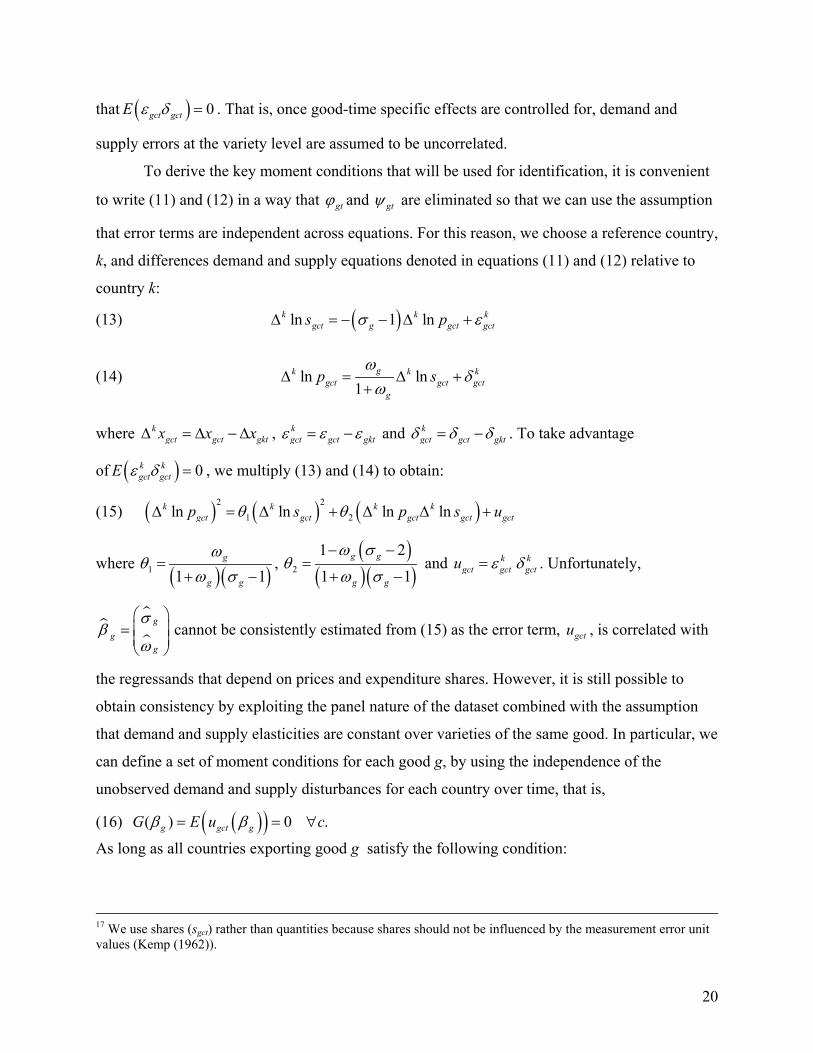
To derive the key moment conditions that will be used for identification, it is convenient

to write (11) and (12) in a way that gtϕ and gtψ are eliminated so that we can use the assumption

that error terms are independent across equations. For this reason, we choose a reference country,

k, and differences demand and supply equations denoted in equations (11) and (12) relative to

country k:

(13) ( )ln 1 lnk k kgct g gct gcts pσ ε∆ = − − ∆ +

(14) ln ln1

gk k kgct gct gct

g

p sω

δω

∆ = ∆ ++

where kgct gct gktx x x∆ = ∆ −∆ , k

gct gct gktε ε ε= − and kgct gct gktδ δ δ= − . To take advantage

of ( ) 0k kgct gctE ε δ = , we multiply (13) and (14) to obtain:

(15) ( ) ( ) ( )2 2

1 2ln ln ln lnk k k kgct gct gct gct gctp s p s uθ θ∆ = ∆ + ∆ ∆ +

where ( )( )1 1 1

g

g g

ωθ

ω σ=

+ −,

( )( )( )2

1 2

1 1g g

g g

ω σθ

ω σ

− −=

+ − and k k

gct gct gctu ε δ= . Unfortunately,

gg

g

σβ

ω

=

cannot be consistently estimated from (15) as the error term, gctu , is correlated with

the regressands that depend on prices and expenditure shares. However, it is still possible to

obtain consistency by exploiting the panel nature of the dataset combined with the assumption

that demand and supply elasticities are constant over varieties of the same good. In particular, we

can define a set of moment conditions for each good g, by using the independence of the

unobserved demand and supply disturbances for each country over time, that is,

(16) ( )( )( ) 0 .g gct gG E u cβ β= = ∀

As long as all countries exporting good g satisfy the following condition:

17 We use shares (sgct) rather than quantities because shares should not be influenced by the measurement error unit values (Kemp (1962)).

21

' '

2 2

2 2

k kgc gc

k kgc gc

ε δ

ε δ

χ χ

χ χ≠

where 2xχ is the variance of x. Equation (16) implies having Vg independent moment conditions

for each good to estimate the two parameters of interest. This condition effectively implies that

the regressands between the two countries c and c’ are not collinear which would not let us solve

the identification problem faced in equation (15). This condition is formally derived in Feenstra

(1991).

For each good g, all the moment conditions that enter the GMM objective function can be

combined to obtain Hansen’s (1982) estimator:

(17) ( ) ( )* *

Bˆ arg ming g gG WG

ββ β β

∈

′=,

where ( )*G β is the sample analog of ( )G β , W is a positive definite weighting matrix to be

defined below, and Β is the set of economically feasible β (i.e., 1; 0g gσ ω> > ). We implement

this estimator by first estimating θ1 and θ2 and then solving for βg as in Feenstra (1994). If this

produces imaginary estimates or estimates of the wrong sign we use a grid search of β s over

the space defined by Β . In particular, we evaluate the GMM objective function for values of σg

∈ [1.05, 131.5] at intervals that are 5 percent apart.18 Standard errors for each parameter were

obtained by boostrapping the grid searched parameters.

18 To make sure that we were using a sufficiently tight grid, we cross-checked these grid-searched parameters with estimates obtained by non-linear least squares as well as those obtained through Feenstra’s original methodology. Using our grid spacing, the difference between the parameters estimated using Feenstra’s methodology and those obtained using the grid search differed only by a few percent for the 65 percent of sigmas for which we could apply Feenstra’s approach. One concern that one might have with this approach is that our grid search sets a maximum σg of 131.5. While this potentially could bias our results because we do not allow for infinite elasticities of substitution, in practice the bias is likely to be quite small. To see this, consider the following example. If σg is 3, fifty percent decline in the lambda ratio (i.e. a doubling in level of varieties) corresponds to a 29 percent decline in the price index; if σg is 20, it corresponds to a 4 percent decline; and if σg is 131.5, a 0.5 percent decline. In other words, constraining the elasticity of substitution to lie below 131.5 will not cause us to identify substantial variety gains or losses when none are present.

22

The problem of measurement error in unit values motivates our weighting scheme. In

particular, there is good reason to believe that unit values calculated based on large volumes are

much better measured than those based on small volumes of imports. In the appendix we show

that this requires us to add one additional term inversely related to the quantity of imports from

the country and weight the data so that the variances are more sensitive to price movements

based on large shipments than small ones. Based on this derivation, all diagonal elements of the

weighting matrix are given by the following expression: 2

1

1 1

gct gctq q

−

−

+

,

where qgct equals the quantity of imports of variety gc in time t, while off-diagonal elements are

zero. Moreover, as in Feenstra (1994), it can be shown that by adding a variable that is

proportional to the variance of the measurement error to (15), the estimates of β are still

consistent, and the problem of measurement error is reduced. This implies that the rank condition

is such that we need data for at least three independent countries to identify consistent estimates

of β .

VI) Results

Our estimation strategy involves four stages. First, we need to obtain estimates of the

elasticity of substitution, σg, by estimating (17). Second, we obtain estimates of how much

variety changed by calculating the λg ratio for every good g (see equation (9)). Third, by

combining our estimates of the elasticity of substitution with the measures of variety for each

good, we obtain an estimate of how much the exact price index for good g moved as a result of

the change variety growth. Finally, we can apply the ideal log weights to the price movements of

each good in order to obtain an estimate of the movement of the aggregate price of imports. Once

we know how much import prices have changed, it is simple to apply equation (10) to calculate

the welfare gain or loss from these price movements.

a) Elasticities of Substitution

We now turn to our estimation of the elasticities of substitution. Given the tens of

thousands of elasticities we estimate, it is impossible to report all of the results here. However,

we can provide some sample statistics that can shed light on the plausibility of our estimates.

23

There are three main priors that we have about these parameters. The first is that as we

disaggregate, varieties are increasingly substitutable. In other words, to give a concrete example,

varieties of the 3-digit category of fruit and vegetables are likely to be less substitutable than

varieties of the 5-digit subcategory that only contains fresh, dried, or preserved apples. Similarly,

varieties within this 5-digit sector are likely to be still less substitutable than varieties in the 7-

digit subcategory containing just fresh apples. Second, we would like the goods with high

elasticities of substitution to correspond to goods that we think of as less differentiated. Finally,

we would like to see that goods traded on organized exchanges have higher elasticities than those

that are not.

Equation (15) can be estimated at various levels of aggregation, and we report sample

statistics for our elasticity estimates in Table 4.19 The results reveal that for both time periods, as

we disaggregate product categories, varieties appear to be closer substitutes. For instance, the

simple average of the elasticities of substitution is 17 for 7-digit (TSUSA) goods during 1972-

1988, while only 7 at the 3-digit level. For the period between 1990 and 2001, the average

elasticity was around 12 for 10-digit (HTS) goods and 4 within 3-digit goods. These differences

are not only large economically, but we can statistically reject the hypothesis that the mean

coefficient for disaggregated goods is the same as that for more aggregated goods.20 In terms of

medians, the elasticity falls less dramatically, from 3.7 and 3.1 at the lowest levels of

disaggregation in the first and second period, respectively, to 2.5 and 2.1. However, in both

periods we can statistically reject that the medians at different levels of aggregation are the same.

In sum, depending on the statistic being used, the elasticities of substitution fall by 33 to 67

percent as we move from highest to lowest level of disaggregation in Table 4. Note also that the

median elasticities of substitution for a given disaggregation level tend to slightly fall over time

and that these differences are statistically significant for the most and least disaggregated data.

19 A clarification can be handy to understand notation. When we estimate σg at the SITC-5 level, then c actually stands for the pair country-TSUSA goods. For instance, if two different TSUSA categories (eg., Apples and Kiwis) belong to a given SITC-5 category (Fresh Fruit), then if the same country (Argentina) exports in the two TSUSA categories, the two pairs (Apples from Argentina and Kiwis from Argentina) will be treated as two different varieties of the same SITC-5 category (Fresh Fruit). 20 We performed this test two ways. First we tested the difference between the means of the estimated σg’s and second we recomputed the means and standard errors after accounting for the censoring of the σg’s due to the grid search. In both cases, we can reject the hypothesis that the means are the same. We reported only the latter.

24

This finding is robust at all product levels, and may represent increasing differentiation among

tradable goods in the latter period.21

Table 5 shows the elasticities of substitution for the 20 largest SITC-3 sectors in US

imports in each of the periods. For the period between 1972 and 1988 the sector with the highest

elasticity of substitution among this group was that of crude oil. The estimated sigma for this

sector was 17.1, fourteen times larger than the sigma for Footwear (σfootwear = 1.2), the sector

with the smallest elasticity in the table. In the latter period, we also find that sectors related to

petroleum have the highest elasticities. More generally, a comparison of elasticities of

substitution across categories shows an intuitive pattern that by and large seem reasonable.

Another way to establish the reasonableness of the estimates is to examine how well they

correspond to other measures of homogeneous and differentiated goods. Rauch (1999) divided

goods into three categories – commodities, reference priced goods, and differentiated goods –

based on whether they were traded on organized exchanges, were listed as having a reference

price, or could not be priced by either of these means. Commodities are probably correlated with

more substitutable goods, but one should be cautious in interpreting commodities as perfect

substitutes or the classification scheme as a strict ordering of the substitutability of goods. For

example, although tea is classified by Rauch as a commodity, it is surely quite differentiated.

Similarly, it is hard to see why a commodity like “dried, salted, or smoked fish” would be more

homogeneous than a referenced priced good like “fresh fish” or a differentiated good like “frozen

fish”. That said, it would be disturbing if we did not find that goods traded on exchanges were

not more substitutable than those that are not.

In order to test this directly, we re-estimated sigmas at the 4-digit level to make them

directly comparable with Rauch’s classification and report the results in Table 6. The most

striking feature of the table is that in both time periods, the average elasticities of substitution are

much higher for commodities than for differentiated or reference priced goods, and the average

elasticities of substitution for reference priced goods are higher than those of differentiated. The

same picture emerges when we look at medians. In all but one case, we can strongly reject the

hypothesis that commodities have the same average and median elasticity as reference priced

goods and differentiated goods in both periods, and we can always reject the hypothesis that

21 The total number of elasticities being estimated at the TSUSA/HTS level is smaller than the total number of TSUSA/HTS available within each period. This responds to the fact that the US imports in a number of categories from a small number of countries and we require at least 3 countries per category to identify parameters.

25

commodities have the same elasticity as the combined set of reference priced and differentiated

goods. This suggests that goods that Rauch classifies as commodities are more likely to have

high elasticities of substitution than goods that are classified as reference priced or differentiated.

b) Growth in Varieties

Now that we have established that our estimates of the elasticities of substitution appear

to be plausible by a number of criteria, we turn to the task of correctly evaluating changes in

variety. One of the major obstacles we face in implementing this procedure is in the calculation

of the λg ratio. Evaluating the impact on price of a new variety is straightforward to do in cases

in which the US imports other varieties of the same TSUSA/HTS category. Unfortunately, the λg

ratio is undefined in cases where there are no common varieties of the TSUSA/HTS category

between the start and end period (i.e., gI =∅ in Proposition 1). The reason why the λg ratio is

undefined is that we cannot value the creation or destruction of a variety without knowing

something about how this affects the consumption of other varieties. To give an example drawn

from our data, we cannot value the invention of CD players for car radios without knowing how

these new goods affected other goods, say, simple car radios. Our solution to this problem is to

assume that whenever a new variety is created within an 7- or 10-digit category for which

gI =∅ then all 7- or 10-digit categories within the same 5-digit category have a common

elasticity of substitution. In other words, in these special cases, the elasticity we use to evaluate

the impact of a new variety being imported on the price level is a weighted average of the

substitutability of other goods and varieties within the same 5-digit category. Similarly, in cases

where the entire 5-digit category is new, we assume a common elasticity at the 3-digit level.22

There are two important implications of this procedure for our results. The first is that the

restriction on the set of goods for which we can calculate λ ratios means that instead of defining

all goods at the TSUSA/HTS level we need to aggregate some of these categories into 5-digit

and 3-digit categories. Because of this necessary aggregation, instead of defining 12347 goods in

the earlier period and 14549 goods for 1990-2001 (i.e., all TSUSA/HTS categories for which we

have σs),23 we can only use 408 and 926 goods (a combination of TSUSA/HTS, SITC-5 and

22 Note also that this approach also eliminates the bias arising from arbitrary re-categorization of goods since new goods simply appear as new varieties of existing goods. 23 These are the numbers of available elasticities of substitution at the TSUSA and HTS level, respectively.

26

SITC-3), respectively. Note, however, that this affects the way varieties are aggregated into

goods but not the total number of varieties being used, which remains unchanged at over 150,000

and 250,000 in the period 1972-1988 and 1990-2001, respectively. Moreover, we need to stress

that this represents vastly more disaggregated data than has been used in the past. Whether this

data limitation introduces a bias into our estimates is harder to assess. Since our calculation of

the λ ratio is robust to many processes that cause existing categories to split or merge, if

statistical agencies are simply changing the definitions of 7- or 10-digit categories within a larger

aggregate, this is unlikely to have an impact on our results. For instance, if a TSUSA good is

split into two goods within the same SITC-5 category, then it is easy to show that λ ratios will be

unaffected by this change (as they should be). By contrast, if the simple number of varieties were

used, then we would wrongly treat this change as an increase in variety.24

Table 7 shows descriptive statistics for the λ ratios of all the 1334 goods used in the

calculation of the aggregate price index, and hence our sample statistics correspond to the

complete set of imported varieties. As the table indicates, even when using λ ratios to measure

variety growth, the typical sector saw the number of imported varieties increase. This table

highlights the importance of using λ ratios rather than relying on count data to measure variety

growth. As shown in Table 1, the total number of varieties per TSUSA more than doubled in the

period between 1972 and 1988 (i.e., N72/N88 = 0.42). In turn, the number of HTS varieties rose by

over 40 percent during 1990-2001. However, when we correctly account for the fact that

varieties are not symmetric in the data, we find that the appropriate magnitudes of variety growth

are substantially smaller. We find that the median measure of variety growth is approximately 25

percent (λ ratio = 0.81) in the period between 1972-1988 and 5 percent (λ ratio = 0.95) in the

latter period. This suggests that by counting the number of varieties one would overestimate the

true growth in variety by a factor of three! Moreover, this underscores the importance of

carefully measuring variety growth when making price and welfare calculations.

c) Import Prices and Welfare

We are now ready to use the elasticities of substitution to evaluate the price effects of

changes in varieties. Aggregating together our λ ratios according to equation (10) yields

24 In the more special case were goods are split into different SITC-5 categories, it is easy to show that the λ ratios would find less growth in varieties than the true growth.

27

estimates of the impact of variety growth on the exact import price index. The results from this

exercise are reported in Table 8. Standard errors on the bias were computed by bootstrapping

each grid-searched estimate of σg 50 times and recomputing the bias for each set of parameters.

Overall, variety growth implies that the variety adjusted unit price for imports fell a precisely

estimated 19.7 percent faster than the unadjusted price between 1972 and 1988 or about 1.4

percentage points per year. Interestingly, the impact of variety growth was much smaller during

the 1990s. Between 1990 and 2001, the growth of varieties meant that the exact price index fell

8.3 percent faster than the unadjusted index over this time period or about 0.8 percentage points

per annum. The lower rate of decline in the later period may reflect the fact that much of the

gains from globalization arising from rise in importance of East Asian trade may have been

realized prior to 1990. If we assume that prices declined in the missing year at the average rate

across the entire sample, we find that throughout the entire period, the growth of varieties

reduces the exact price relative to conventionally measured import price index by 28.0 percent.

It is difficult to find a benchmark with which to compare our results. We are not aware of

any study that measures the impact of variety on aggregate prices, and the papers that study a

single good at the micro-level (or at most a few goods) are not suitable for this comparison.

Given the lack of aggregate effects of variety in the literature, we will use as a reference the

effects that other sources of bias (quality change, outlet substitution, etc.) have on the overall

consumer price index. In mid-1995 a commission was appointed to study the potential biases in

the existing measurement of the Consumer Price Index. This CPI Commission concluded that the

change in the consumer price index overstates the change in the cost of living by about 1.2

percentage points per year (Boskin et al., 1996). Several sources of bias are considered, but the

main source is the incorrect measurement of quality change of products. The effect of quality

change alone can account for about 0.6 percentage points in the overall index. These numbers

suggests that the bias that we find in the import price index only as a result of the unaccounted

variety growth is very large. That is, the bias due to variety growth in the import price index is

almost twice as large as the bias induced by quality change in the overall price index and as large

as the total bias from all sources.

We now turn to calculating the welfare effect of the fall in the US exact import price. Not

surprisingly, the magnitude of the welfare gain from this fall hinges on the functional forms

underlying the Dixit-Stiglitz structure and cannot be general. If elasticities of substitution are not

28

constant or if marginal costs are not fixed, theory suggests that one can obtain higher or lower

estimates of the gains from variety. Although our estimate of the impact of imported varieties on

import prices is correct for any domestic production structure, we cannot translate this into a

welfare gain without making explicit assumptions about the structure of domestic production.

Our choice is to assume the same structure of the US economy as in Krugman (1980). We do this

for two reasons. First, since this is the dominant model of varieties, it provides a useful

benchmark for understanding the potential welfare gains. Second, we lack the necessary data and

model of the economy’s input-output linkages to estimate variants of the monopolistic

competition model in which there are more complex interactions between imported and domestic

varieties.

These concerns notwithstanding, one of the strengths of our analysis is that we can be

almost completely agnostic about the causes of the increase in imported varieties. Presumably

the causes are some combination of reductions in trade costs and growth in foreign output.

Moreover, since we will use ideal weights to calculate the impact of price changes on welfare, a

shift in preferences in favor of imports will not bias our welfare calculations.25

Equation (10) shows that the percent change in welfare that results from changes in

varieties in imported goods can be calculated using the inverse of the product of the weighted λ

ratios raised to the fraction of imported goods in total consumption goods, (1-α). In particular,

we use the ideal import share in each period, 6.7 percent for 1972-1988 and 10.3 percent for

1990-2001, respectively, together with the information in Table 8 to obtain the gains in welfare

due to variety. We find that real income has increased by 2.6 percent solely as a result of the

changes in varieties. Around 1.8 percentage points accrue to the earlier period. These gains from

variety are 4 to 10 times larger than the estimated gains from eliminating protectionism (e.g.,

Krugman (1990)and Tarr and Morkre (1984)) and around 10 times larger than the estimated

gains from eliminating business cycles (Alvarez and Jermann (2000)).

d) Robustness of results to alternative assumptions

In the previous section we computed the impact of variety growth of US imports on

aggregate welfare. Our computation required several weaker assumptions than those present in

previous numerical exercises. First, we do not require that varieties or goods have equal shares in

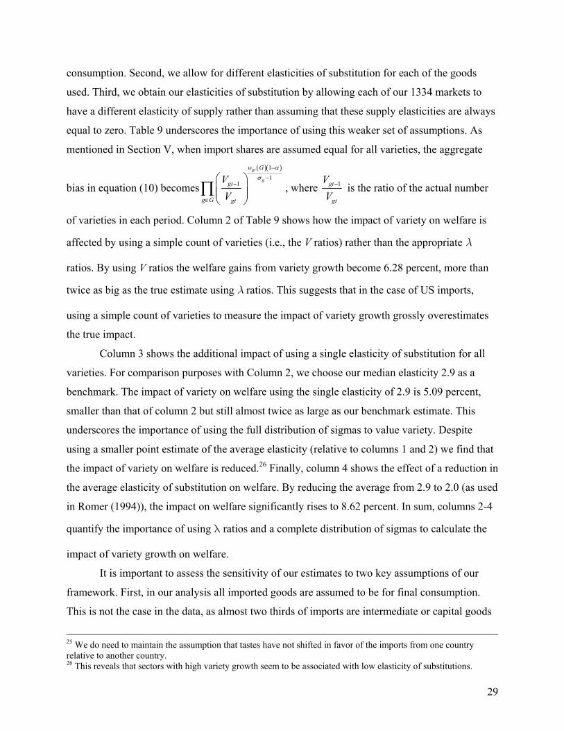
29

consumption. Second, we allow for different elasticities of substitution for each of the goods

used. Third, we obtain our elasticities of substitution by allowing each of our 1334 markets to

have a different elasticity of supply rather than assuming that these supply elasticities are always

equal to zero. Table 9 underscores the importance of using this weaker set of assumptions. As

mentioned in Section V, when import shares are assumed equal for all varieties, the aggregate

bias in equation (10) becomes

( )( )11

1

gt

g

w G

gt

g G gt

VV

ασ

−

−−

∈

∏ , where 1gt

gt

VV

− is the ratio of the actual number

of varieties in each period. Column 2 of Table 9 shows how the impact of variety on welfare is

affected by using a simple count of varieties (i.e., the V ratios) rather than the appropriate λ

ratios. By using V ratios the welfare gains from variety growth become 6.28 percent, more than

twice as big as the true estimate using λ ratios. This suggests that in the case of US imports,

using a simple count of varieties to measure the impact of variety growth grossly overestimates

the true impact.

Column 3 shows the additional impact of using a single elasticity of substitution for all

varieties. For comparison purposes with Column 2, we choose our median elasticity 2.9 as a

benchmark. The impact of variety on welfare using the single elasticity of 2.9 is 5.09 percent,

smaller than that of column 2 but still almost twice as large as our benchmark estimate. This

underscores the importance of using the full distribution of sigmas to value variety. Despite

using a smaller point estimate of the average elasticity (relative to columns 1 and 2) we find that

the impact of variety on welfare is reduced.26 Finally, column 4 shows the effect of a reduction in

the average elasticity of substitution on welfare. By reducing the average from 2.9 to 2.0 (as used

in Romer (1994)), the impact on welfare significantly rises to 8.62 percent. In sum, columns 2-4

quantify the importance of using λ ratios and a complete distribution of sigmas to calculate the

impact of variety growth on welfare.

It is important to assess the sensitivity of our estimates to two key assumptions of our

framework. First, in our analysis all imported goods are assumed to be for final consumption.

This is not the case in the data, as almost two thirds of imports are intermediate or capital goods

25 We do need to maintain the assumption that tastes have not shifted in favor of the imports from one country relative to another country. 26 This reveals that sectors with high variety growth seem to be associated with low elasticity of substitutions.

30

and not final consumption goods. As noted by Romer (1994), however, the Dixit-Stiglitz

structure allows for new varieties to be modeled either as consumption goods, as in Grossman

and Helpman (1991), or as intermediate inputs in production, as in Romer (1990), with no

fundamental change in the underlying economic analysis. In other words, treating the share of

imported intermediate goods as final consumption does not necessarily bias our estimates. The

case of capital goods is different. While consumption varieties only offer a static gain, the

potential gains from variety growth in capital goods can have persistent effects in time. This has

the potential of magnifying the effects of variety growth on welfare relative to our “static”

results. Therefore, treating capital goods as final consumption seems to imply that we are

understating the true gains from variety.

The second assumption that is important for our results is that of Krugman’s (1980)

production structure. This structure assumes that the number of domestic varieties are unaffected

by new foreign varieties (as in Feenstra (1992), Romer (1994) and Klenow and Rodriguez

(1997)). However, if domestic varieties were affected by imported varieties, then our welfare

calculations would change. Unfortunately, we lack the data to relax this assumption while still

maintaining a CES structure. However, we can still allow for a more flexible structure if we

assume a linear demand system.27

In order to implement this, we assume that the elasticity of substitution between domestic

and foreign varieties is infinity. In this extreme case, imports perfectly displace domestic

production and there can be no price difference between domestic and imported production. We

assume further that all varieties are consumed in all time periods. However, it is important to

realize that an import price index that computes price changes by comparing the prices of goods

that are imported in two periods will not capture price drops of goods that imported in the second

period but not the first. In other words, if the price of an imported good falls from a price at

which the US demands nothing to a price at which the US imports a positive quantity, the US

import price index should fall and US welfare should rise, but none of this would be captured in

a conventional import price index built on existing goods.

27 The relationship between domestic and foreign varieties is complex to model, but several different strategies exist in the literature. Rutherford and Tarr (2002) develop a model for a small open economy in which domestic varieties are partially substituted by imported varieties when tariffs on imported goods fall. By contrast, in a model with vertical specialization and differentiated products, increases in imported intermediate varieties can lead to new domestic varieties.

31

The magnitudes of these price and welfare changes can be computed by considering

Figure 1. Here we assume that the good gc, e.g. French red wine, is a perfect substitute for a

domestic version of “French” red wine although it is not a perfect substitute for, say, Italian red

wine. It is therefore convenient to maintain the gc subscript even though both the US and France

can produce “French” red wine. In this case, a price drop from 0gcp to 1

gcp would induce imports

to rise from zero to M1. Similarly, a rise in price from 1gcp to 0

gcp would cause imports to fall

from M1 to zero. If we can assume that the demand and supply curves can be approximated by

lines in the region of interest, the change in welfare arising from the price change associated with

entry or exit of imports in the market can be written as

(18) 12 gc gcp M− ∆ ∆

A conventional price index would not measure this price fall and hence this welfare gain because

conventional price indices do not contain information about new and disappearing goods.

We compute these virtual price equations by returning to our import demand equation.

By definition, our import demand elasticity can be written as

(19) 1 gc gcg

gc gc

dM pdp M

σ− =

If we linearize our import demand curve around M1 we have

(20) 1

1

11

gcgc

g gc

pM

µσ

=−

where µgc is the slope of the demand curve described by equation (21). In this case the

reservation price, p0 can be written as

(21) 1 0 1 0 1 1 1 111gc gc gc gc gc gc gc gc gc

g

p p M p p M pµ µσ

= + ⇔ = − = − −

Using equation (21) we can compute the implied import price changes that arise when

goods start and stop being imported. We implement equation (21) by using the same elasticities

used in the previous welfare calculation. We then compute the implied welfare gain or loss in

each market due to the appearance or disappearance of new varieties according to equation (18),

and sum across all markets. The ratio of 0gcp / 1

gcp corresponds to the ratio of the virtual price (i.e.

the price at which imports are zero) relative to the price we observe in the market. Using this

32

formula we estimate virtual prices are on average 2.0 times higher than observed prices in the

earlier time period and 2.3 times higher in the later period. Since Hausman (1994) in his study of

breakfast cereals argues that a virtual price of 2 times the observed sales price is a “reasonable

estimate”, we can have confidence that our elasticities are sensible in general.

Turning to welfare, we next use equation (18) to compute the welfare gain and loss in

each market. Interestingly, our estimates based on this procedure reveal a net welfare gain from

variety change between 1972 and 2001 of 4.1 percent of GDP which is actually slightly larger

than our estimate in the CES structure of 2.6 percent! This suggests that even if we allow

domestic goods to be perfect substitutes for foreign goods and linearize the demand system, we

still observe substantial gains from unmeasured price drops arising from new imports.

Finally, Peter Schott (2004) has convincingly argued that there are important quality

differences associated with the per capita GDP of the exporting country. To the extent that these

quality differences are constant across time, our methodology will be unaffected. However, he

presents evidence that these differences may contain a time-series component. If this is true our

estimates may be biased because quality shocks may be correlated with supply shocks. In order

to correct for this possibility we added a per capita GDP term into equation (11) to account for

the fact that import demand shocks may be correlated with export supply shocks. When we re-

derived our estimating equation (15) this introduced two additional terms which we added when

obtaining the point estimates. The resulting elasticities were extremely close to the ones reported

in this paper indicating that quality changes are probably not biasing our results.28

VII) Conclusion

Understanding the impact of new products and the growth in varieties on economies has

been one of the central questions in international economics, regional economics, and

macroeconomics. Until now, attempts to estimate magnitude of these effects have been limited

to extremely careful econometric studies of particular goods and attempts to calibrate standard

models. The failure to obtain credible estimates of the impact of new goods and varieties on

prices and welfare at the national level has stemmed from the difficulty of implementing careful

econometric studies of particular markets more broadly and from the implausibility of many

assumptions underlying calibration exercises.

28 These results are available from the authors upon request.

33

This paper is the first attempt to implement a methodology that estimates all of the

parameters necessary to calculate an exact price index and perform welfare calculations at the

national level. This, of course, does not obviate the need for careful econometric studies of entry

in particular markets. Indeed, we see this work as complementary to ours. In markets where

sufficient data exist to obtain better estimates of price effects due to entry, one should do so.

Indeed, one could imagine more precise estimates of the impact of new goods and varieties

arising from a hybrid technique in which certain markets are modeled in detail and others are

modeled according to our implementation of the Feenstra index. Whether that would

substantially alter our results is impossible to say, but our results are robust to a wide range of

model specifications and assumptions.

Our results indicate that the effect of new goods and varieties on the US economy is

large. By ignoring these effects, the US import price index overstates import price inflation by

1.2 percentage points per year. If the bias in the CPI is comparable to the bias in the import price

index, then this suggest that the biases identified in this paper are not only more important than

quality adjustments, they are more important than all other biases combined. Obviously more

work needs to be done to understand whether the biases in the import price index are similar in

magnitude to those in the CPI, but the results suggest that there is potential for very large effects.

Finally, our results suggest that globalization has had substantial impacts on welfare

through the import of new varieties. US welfare is 2.6 percent higher due to gains accruing from

the import of new varieties. An important qualification is that our estimates are obtained by

assuming the US economy can be modeled as in Krugman (1980). While this is a sensible

benchmark, there clearly is a need for better modeling and estimation of dynamic and input-

output effects arising from increases the number of varieties. Even so, our estimation indicates

that the gains from trade first suggested by Krugman a generation ago are quite important in

reality.

34

References

Anderson (1979) “A Theoretical Foundation for the Gravity Equation,” American Economic Review, Vol 69(1), pp. 106-116

Armington, Paul S. “A Theory of Demand for Products Distinguished by Place of Production.”

International Monetary Fund Staff Papers, March 1969, 16(1), pp. 159-78. Alvarez, Fernando and Urban Jermann (2000) “Using Asset Prices to Measure the Cost of

Business Cycles, University of Chicago, mimeo. Bils, M. and Klenow, P. J. (2001) “The Acceleration of Variety Growth” American Economic

Review, 91(2), pp. 274-80. Boskin, M., E. Dulberger, R. Gordon, Z. Griliches and D. Jorgenson (1996) "Toward a More

Accurate Measure of the Cost of Living: Final Report to the Senate Finance Committee," Washington, DC, U.S. Government Printing Office, for the U.S. Senate Committee on Finance, December.

Broda, Christian and David E. Weinstein (2004) ““Variety Growth and World Welfare,”

American Economic Review Papers and Procedings, 94(2), pp. 139-145. Brown, Drusilla, Alan V. Deardorff, and Robert M. Stern, "Modeling Multilateral Trade

Liberalization in Services," Jul. 6, 1995. Asia-Pacific Economic Review, April, 1996. Diewert, W. E. “Exact and Superlative Index Numbers.” Journal of Econometrics, May 1976,

4(2), pp. 115-45.

Dixit, Avinash K. and Stiglitz, Joseph E. “Monopolistic Competition and Optimum Product Diversity.” American Economic Review, June 1977, 67(3), pp. 297-308.

Eaton, Jonathan and Kortum, Samuel. “Technology, Geography, and Trade.” Econometrica,

September 2002, 70(5), pp. 1741-79. Feenstra, Robert C. “How Costly Is Protectionism?” Journal of Economic Perspectives, Summer

1992, 6(3), pp. 159-78. _____. “New Product Varieties and the Measurement of International Prices.” American

Economic Review, March 1994, 84(1), pp. 157-77. _____. “U.S. Imports, 1972-1994: Data and Concordances.” National Bureau of Economic

Research Working Paper No. 5515, March 1996. Fujita, Masahisa; Krugman, Paul; Venables, Anthony J. The Spatial Economy: Cities, Regions,

and International Trade. Cambridge and London: MIT Press, 1999.

35

Gallaway, M. P., C. A. McDaniel and S. A. Rivera (2003), "Short-Run and Long-Run Industry-Level Estimates of U.S. Armington Elasticities," North American Journal of Economics and Finance, 14(1), 49-68.

Grossman, Gene M. and Helpman, Elhanan. Innovation and Growth in the Global Economy,

Cambridge, Mass. and London: MIT Press, 1991. _____. “Product Development and International Trade.” Journal of Political Economy,

December 1989, 97(6), pp. 1261-83. Griliches, Zvi and Hausman, Jerry A. “Errors in Variables in Panel Data.” Journal of

Econometrics, February 1986, 31(1), pp. 93-118. Hansen, Lars Peter. “Large Sample Properties of Generalized Method of Moments Estimators.”

Econometrica, July 1982, 50(4), pp. 1029-54. Hausman, Jerry A. “Exact Consumer's Surplus and Deadweight Loss.” American Economic

Review, Sept. 1981, 71(4), pp. 662-76.

_____. “Valuing the Effect of Regulation on New Services in Telecommunications.” Brookings Papers on Economic Activity, Microeconomics, 1997, 0(0), pp. 1-38.

_____. “Valuation of New Goods Under Perfect and Imperfect Competition. The Economics of

New Goods.” National Bureau of Economic Research Studies in Income and Wealth, Vol. 58. Chicago and London: University of Chicago Press, 1997, pp. 209-37.

Helpman, Elhanan and Krugman, Paul R. Market Structure and Foreign Trade: Increasing

Returns, Imperfect Competition, and the International Economy. Cambridge, Mass. and London: MIT Press, 1985.

Helpman, Elhanan and Krugman, Paul R. Trade policy and market structure. Cambridge, Mass.

and London: MIT Press, 1989. Klenow, Peter J. and Andres Rodriguez-Clare. “Quantifying Variety Gains from Trade

Liberalization” mimeo September 1997. Krugman, Paul R. “Increasing Returns, Monopolistic Competition, and International Trade.”

Journal of International Economics, Nov. 1979, 9(4), pp. 469-79.

_____. “Scale Economies, Product Differentiation, and the Pattern of Trade.” American Economic Review, Dec. 1980, 70(5), pp. 950-59.

_____. Rethinking International Trade, Cambridge: The MIT Press, 1990.

Lancaster, Kelvin. “Socially Optimal Product Differentiation.” American Economic Review,

September 1975, 65(4), pp. 567-85.

36

Leamer, Edward E. “Is It a Demand Curve, or Is It a Supply Curve? Partial Identification through Inequality Constraints.” Review of Economics and Statistics, August 1981, 63(3), pp. 319-2.

Rauch, James E. “Networks versus Markets in International Trade.” Journal of International

Economics, June 1999,48(1), pp. 7-35. Rigobon, Roberto and Sack, Brian. “Measuring the Reaction of Monetary Policy to the Stock

Market.” Quarterly Journal of Economics, May 2003,118(2), pp. 639-69. _____. “On the Measurement of the International Propagation of Shocks.” National Bureau of

Economic Research Working Paper No. 7354, September 1999.

Romer, Paul M. “Capital, Labor, and Productivity.” Brookings Papers on Economic Activity, Special Issue, 1990, 0(0), pp. 337-67.

_____. “New Goods, Old Theory, and the Welfare Costs of Trade Restrictions.” Journal of

Development Economics, February 1994, 43(1), pp. 5-38. Rutherford, Thomas F. and Tarr, David G. “Trade Liberalization, Product Variety and Growth in

a Small Open Economy: A Quantitative Assessment.” Journal of International Economics, March 2002, 56(2), pp. 247-72.

Sato, Kazuo. “The Ideal Log-Change Index Number.” Review of Economics and Statistics, May

1976, 58(2), pp. 223-28.

Schott, Peter. “Across-Product versus Within-Product Specialization in International Trade.” Quarterly Journal of Economics, May 2004 119(2):647-678.

Spence, Michael. “Product Differentiation and Welfare.” American Economic Review, May

1976, 66(2), pp. 407-14. Tarr, David. and M. Morkre. Aggregate Costs to the United States of Tariffs and Quotas on Imports,"

General Tariff Cuts and Removal of Quotas on Automobiles, Steel, Sugar, and Textiles, Bureau of Economics Report to the Federal Trade Commission, U.S. Government Printing Office, December 1984.

Yi, Kei-Mu. “Can Vertical Specialization Explain the Growth of World Trade?” Journal of Political

Economy, February 2003, 52-102.

37

Figure 1

Domestic Supply

Domestic Demand

0gcp

1gcp

Imports (M1)

38

Appendix

Biases and Weighting in the Presence of Measurement Error

Let pgct be the unit value of a variety that we have in our dataset (e.g. French Red Wine) and pgcti is the unit value of a particular product contained in that variety (e.g. a bottle of French Red Wine). If we assume that the log of geometric mean price of a variety is approximately equal to the log of the arithmetic mean, we have

(22)

1

ln ln lngct

gcti qi

gct gctiigct

pp p

q

≡ ≈

∑∏

where qgct is the quantity of imported variety gc in time t.

Assume that measure product prices with an iid error such that gcti gcti gctip p ζ= , where

gctip is the true price and pgcti is the measured price. In this case

2

'

var(ln )cov(ln , ln ) 0 ', ,

gcti

gcti gc sj c c t s i jζ χ

ζ ζ

≡

= ∀ ≠ ≠ ≠

(23)

2ln

1

2 22 2

var ln

1 1 1var ln var ln

gct

gct

gctii

pgct

q

gcti gcti gctii gct gct gct

p

q

p p qq q q

χ

χ χ

≡

≈ = = =

∑

∑∏

Now

(24) ( ) 21

1

1 1var ln lngct gctgct gct

p pq q

χ−−

− = +

This implies that we should add a term equal to

(25) 2

1

1 1

gct gctq qχ

−

+

to the right-hand side of equation (15) where 2χ is a parameter to be estimated. A related but distinct issue concerns heteroskedasticity in the data. Every data point comprising the left-hand side of equation (15) is an estimate of the variance. However, if the prices are measured with error, then so are our sample variances. Using equation (24), we can correct for this heteroskedasticity by realizing that

39

(26)

( )

( )

21

1

2

2

1

1 1var var ln ln var

1 1var

gct gctgct gct

gct gct

p pq q

q q

χ

χ

−−

−

− = +

+

where ( )2var χ corresponds to the variance of the variance. This implies that we weight the data by

2

1

1 1

gct gctq q

−

−

+

It is worth nothing that if qgct = qgct-1 the terms in parentheses in equations (25) and (26) become constants. This is the specification estimated in Feenstra (1994). Our algebra can thus be seen as a generalization Feenstra’s approach that allows for measurement error to depend on the quantity of varieties.

US Imports 1972-1988

Year Number of

Goods

Median Number of Exporting Countries

Average Number of Exporting Countries

Total Number of Varieties (country-

good pairs)Share of Total US

Imports in year(1) (2) (3) (4) (5) (6)

All 1972 goods 1972 7731 6 9.7 74667 1.00All 1988 goods 1988 12822 9 13.6 173937 1.00Common 72-88 1972 4171 6 8.7 36191 0.48Common 72-88 1988 4171 10 13.5 56183 0.321972 not in 1988 1972 3560 7 10.8 38476 0.521988 not in 1972 1988 8651 8 13.6 117754 0.68

Year Number of

Goods

Median Number of Exporting Countries

Average Number of Exporting Countries

Total Number of Varieties (country-

good pairs)Share of Total US

Imports in year(1) (2) (3) (4) (5) (6)

All 1990 goods 1990 14572 10 12.5 182375 1.00All 2001 goods 2001 16390 12 15.8 259215 1.00Common 90-01 1990 10636 10 12.4 132417 0.73Common 90-01 2001 10636 13 16.3 173776 0.671990 not in 2001 1990 3936 10 12.7 49958 0.272001 not in 1990 2001 5754 11 14.8 85439 0.33

Notes: For the period 1972-1988 goods are defined at the 7-digit TSUSA level. For the latter period, 10-digit HTS data is used. Source: NBER CD-ROM and http://data.econ.ucdavis.edu/international/usixd/wp5514d.html

Table 1: Variety in US Imports (1972 - 2001)

US Imports 1990-2001

Country 1972 1988 1990 2001JAPAN 1 1 3 7UKINGDOM 2 4 4 3GERMAN 3 3 2 2CANADA 4 2 1 1FRANCE 5 6 5 6ITALY 6 5 6 5SWITZLD 7 11 11 11HONGKONG 8 9 12 16NETHLDS 9 13 13 14TAIWAN 10 7 7 9SPAIN 11 14 15 12BEL_LUX 12 15 14 15MEXICO 13 12 10 8SWEDEN 14 17 16 19DENMARK 15 22 21 23AUSTRIA 16 18 18 21INDIA 17 19 23 13KOREA_S 18 8 9 10BRAZIL 19 16 17 18AUSTRAL 20 20 20 20ISRAEL 21 21 22 22PORTUGAL 22 26 28 32NORWAY 23 31 31 37IRELAND 24 27 26 28FINLAND 25 28 30 31COLOMBIA 26 33 34 35PHIL 27 25 25 26CHINA 28 10 8 4ARGENT 29 29 29 39GREECE 30 38 44 47

Notes: Top 30 countries in 1972 included. Same notes as in table 1 apply.

Table 2: Ranking in terms of Number of Goods Imported by US

Ranking in year:

Table 3: Country Contribution to Growth in US Varieties (1972-1988 / 1990-2001)

CountryContribution 1972-1988

Average Share of US Imports (1) Country

Contribution 1990-2001

Average Share of US Imports (1)

CHINA 4.8% 1.0% CHINA 5.7% 6.0%TAIWAN 4.4% 4.0% INDIA 4.4% 0.7%KOREA_S 4.4% 2.9% MEXICO 3.7% 8.8%CANADA 4.2% 22.7% SPAIN 2.9% 0.6%ITALY 4.0% 2.9% S_AFRICA 2.6% 0.4%GERMAN 3.8% 6.9% ITALY 2.6% 2.3%FRANCE 3.8% 2.6% INDONES 2.5% 0.8%JAPAN 3.6% 18.4% CANADA 2.5% 18.7%UKINGDOM 3.5% 4.7% TURKEY 2.3% 0.3%HONGKONG 3.1% 2.3% THAILAND 2.3% 1.2%MEXICO 3.0% 4.0% AUSTRAL 2.1% 0.7%SWITZLD 2.6% 1.1% FRANCE 2.1% 2.7%BRAZIL 2.6% 1.9% KOREA_S 2.0% 3.4%NETHLDS 2.2% 1.1% BEL_LUX 1.9% 0.9%THAILAND 2.2% 0.5% POLAND 1.8% 0.1%SINGAPR 1.9% 1.1% MALAYSIA 1.8% 1.5%

Notes: A US variety is defined as a TSUSA-country pair in 1972-1988 and HTS-country pair in 1990-2001. (1) Log ideal weights used as average shares (see text for a definition). Same notes as Table 1 apply.

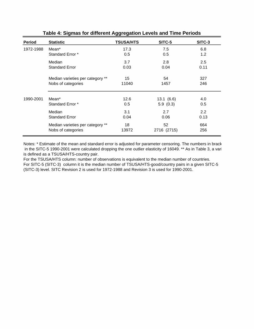
Table 4: Sigmas for different Aggregation Levels and Time Periods

Period Statistic TSUSA/HTS SITC-5 SITC-31972-1988 Mean* 17.3 7.5 6.8

Standard Error * 0.5 0.5 1.2

Median 3.7 2.8 2.5Standard Error 0.03 0.04 0.11

Median varieties per category ** 15 54 327Nobs of categories 11040 1457 246

1990-2001 Mean* 12.6 13.1 (6.6) 4.0Standard Error * 0.5 5.9 (0.3) 0.5

Median 3.1 2.7 2.2Standard Error 0.04 0.06 0.13

Median varieties per category ** 18 52 664Nobs of categories 13972 2716 (2715) 256

Notes: * Estimate of the mean and standard error is adjusted for parameter censoring. The numbers in brack in the SITC-5 1990-2001 were calculated dropping the one outlier elasticity of 16049. ** As in Table 3, a variis defined as a TSUSA/HTS-country pair. For the TSUSA/HTS column: number of observations is equivalent to the median number of countries. For SITC-5 (SITC-3) column it is the median number of TSUSA/HTS-good/country pairs in a given SITC-5 (SITC-3) level. SITC Revision 2 is used for 1972-1988 and Revision 3 is used for 1990-2001.

SITC-3 Sigma Average Share (in %) Descriptions

333 17.1 29.6 CRUDE OIL FROM PETROLEUM OR BITUMINOUS MINERALS781 1.6 8.3 MOTOR CARS & OTH MOTOR VEHICLES334 9.0 5.4 OIL (NOT CRUDE) FROM PETROL & BITUM MINERALS ETC341 5.7 2.4 FISH, FRESH OR CHILLED (EXC FILLETS & MINCED FISH)71 2.5 2.0 COFFEE AND COFFEE SUBSTITUTES776 1.6 1.6 THERMIONIC, COLD CATHODE, PHOTOCATHODE VALVES ETC.641 6.7 1.6 PAPER AND PAPERBOARD851 1.2 1.4 FOOTWEAR681 1.4 1.2 SILVER, PLATINUM & OTHER PLATINUM GROUP METALS674 11.8 1.2 IRON & NA STEEL FLAT-ROLLED PRODUCTS, CLAD, ETC.

SITC-3 Sigma Average Share (in %) Descriptions

781 3.0 10.6 MOTOR CARS & OTH MOTOR VEHICLES333 22.1 7.0 CRUDE OIL FROM PETROLEUM OR BITUMINOUS MINERALS776 1.2 6.4 THERMIONIC, COLD CATHODE, PHOTOCATHODE VALVES ETC.752 2.2 5.7 SPICES (EXCEPT PEPPER AND PIMENTO)784 2.8 3.4 PARTS AND ACCESSORIES OF MOTOR VEHICLES, ETC851 2.4 2.0 FOOTWEAR764 1.3 1.9 TELECOMMUNICATIONS EQUIPMENT, N.E.S. & PTS, N.E.S.713 2.7 1.8 COFFEE/SUBT EXTRACTS/ESSENCES/CONCENTRATES & PREPS845 6.7 1.8 ARTICLES OF APPAREL OF TEXTILE FABRICS NES641 2.1 1.7 PAPER AND PAPERBOARD

Notes: SITC-3 Revision 2 (Revision 3) codes are used for the period 1972-1988 (1990-2001). Shares are simple averages of start anend years. Also see notes from Table 5. (*) Corresponds to the Revision 3 SITC 3 or 5 name of that category.

Period 1972-1988

Table 5: Sigmas for the 20 SITC-3 Sectors with the Largest Import Share by Period

Period 1990-2001

Commodity Reference Priced Differentiated

Mean 15.3 7.8 5.2Standard Error 3.0 1.5 0.8Test if different than Commodity 0.01 0.00(p-value)

Median 4.8 3.4 2.5Standard Error 0.4 0.3 0.1Test if different than Commodity 0.01 0.00(p-value)

Mean 11.6 4.9 4.7Standard Error 3.0 0.6 1.0Test if different than Commodity 0.01 0.01(p-value)

Median 3.5 2.9 2.1Standard Error 0.6 0.2 0.1Test if different than Commodity 0.14 0.00(p-value)

Note: p-values for 1-sided t-test reported. (1) p-value for a joint test of referenced anddifferentiated vs commodity goods.

Table 6: Estimated Sigmas and Rauch Liberal Classification

Rauch's Classification of Goods:

1972-1988 (4-digit)

1990-2001 (4-digit)

Period Statistic

Combination of TSUSA/HTS - SITC5 -

SITC3 used

Implied by Count Data in

Table 1

1972-1988 Percentile 5 0.06Median 0.81 0.42Percentile 95 2.00Nobs 408

1990-2001 Percentile 5 0.34Median 0.95 0.70Percentile 95 1.80Nobs 926

Notes: See text for definitions.

Table 7: Descriptive Statistic of Lambda Ratios

End-point Ratio Average Per-annum Ratio

1972-1988 0.803 0.986[0.790 , 0.835]

1990-2001 0.917 0.992[0.907 , 0.941]

1972-2001 0.720 0.988[0.705 , 0.771]

Notes: This table shows the estimated values of equation (12) by period. (1) Forthe period between 1988 and 1990 the average per-annum rate was applied.Bootstrapped 90th percent confidence intervals in brackets.

Ratio between Aggregate Exact Price Index including Variety and the Aggregate Conventional Price Index

Table 8: The Impact of Variety in US Import Prices

Benchmark EstimateEquality of Import

SharesSingle Gravity

SigmaSmaller Median

Sigma(1) (2) (3) (4)

Number of Sigmas Used 1334 1334 1 1

Median Sigma 2.9 2.9 2.9 2.0Median [Percentile 5, Percentile 95] [2.1 , 5.2]

Average Sigma 6.5 6.5 2.9 2.0

Lambda Ratio (L) or Count Data (N) L N N N

Average Share (in percent) (1) 8.5 8.5 8.5 8.5

Welfare Impact 2.59 6.28 5.09 8.62[2.01 , 2.84]

Notes: (1) For expositional purposes, we present the weighted average share of imports between the periods 1972-1988 and 1990-2001. Calculations are based on each period's average share and not on this weighted average. (2)

Table 9: Welfare Comparisons