globe claritas v6.0 2dmarine tutorial 4 clar… · · 2015-09-14using this tutorial ... 1.1...
TRANSCRIPT

2D MARINE PROCESSING
Version 6

GLOBE Claritas 2D Marine Processing
©GNS Science Page i
TABLE OF CONTENTS
1. Using This Tutorial ................................................................................................... 1 1.1 Seismic Line TRV-434 ...................................................................................... 2
2. GETTING STARTED WITH GLOBE CLARITAS ...................................................... 3 2.1 Objectives ........................................................................................................ 3 2.2 The GLOBE Claritas Launcher......................................................................... 3 2.3 Getting Help ..................................................................................................... 4 2.4 GLOBE Claritas Projects .................................................................................. 5
3. INITIAL DATA QC USING XSJE AND XVIEW ......................................................... 8 3.1 Objectives ........................................................................................................ 8 3.2 XSJE: The Seismic Processing Job Flow Editor .............................................. 8 3.3 Adding, Deleting and Flipping Modules .......................................................... 13 3.4 Configuring Different Display Modes .............................................................. 14 3.5 Initial Data QC: XVIEW Analysis and Zoom Windows ................................... 16
4. SHOT-BASED PRE-PROCESSING AND NOISE SUPPRESSION ........................ 17 4.1 Objectives ...................................................................................................... 17 4.2 Refraction Mute Picking in SV ........................................................................ 18
4.2.1 Parameter Files: The XSDE Editor ...................................................... 21 4.2.2 Checking the Mute Application: REPEAT Panels, IF and ENDIF ....... 22
4.3 AMPLITUDE RECOVERY TESTS WITH REPEAT ....................................... 24 4.4 Swell Noise Analysis and Suppression Tests, Difference Plots ..................... 29 4.5 Application of FK Filters, detecting spikes and managing amplitudes ........... 31
4.5.1 Using AREAL to Monitor Amplitudes or Find Spikes ........................... 34 4.6 Building a Shot Processing “Production” Workflow ........................................ 35 4.7 Quality Control Processing Flows .................................................................. 36
4.7.1 AREAL QC and Trace Editing ............................................................. 39
5.0 SORT TO CDP AND DECONVOLUTION ............................................................... 41 5.1 Objectives: ..................................................................................................... 41 5.2 Creating a Brute Stack ................................................................................... 41
5.2.1 Hardcopy of the Brute Stack ............................................................... 42 5.3 Minimum Phase Conversion and the Wavelet tool ......................................... 44 5.4 Viewing Autocorrelation Functions ................................................................. 47 5.5 Testing Weiner Deconvolution before Stack .................................................. 48
5.5.1 Applying Deconvolution and Sorting the Data ..................................... 52 5.5.2 Checking the Results .......................................................................... 53
6. VELOCITY ANALYSIS ............................................................................................ 54 6.2 Objectives: ..................................................................................................... 54
6.2.1 Picking Velocities in CVA .................................................................... 54 6.3 Picking NMO stretch Mutes ............................................................................ 64 6.4 Checking Velocities and Mutes with SV ......................................................... 65
6.4.1 Creating a QC stack ............................................................................ 67
7. IMPROVING VELOCITY ANALYSIS: ANTI-MULTIPLE AND PRESTM ................ 67 7.1 Objectives: ..................................................................................................... 67 7.2. RADON Demultiple Theory ............................................................................ 67
7.2.1 Testing and Applying RADON Demultiple ........................................... 68 7.3 Pre-stack Time Migration ............................................................................... 73 7.4 Second Pass Velocity Analysis ...................................................................... 79 7.5 Iterative Migrations ......................................................................................... 79

GLOBE Claritas 2D Marine Processing
©GNS Science Page ii
8. FINALISATION ........................................................................................................ 80 8.1 Objectives: ..................................................................................................... 80 8.2 Testing Deconvolution after Stack .................................................................. 80 8.3 Random Noise Attenuation Tests ................................................................... 81 8.4 Testing Filters ................................................................................................. 82 8.5 Testing Final Scaling ...................................................................................... 83 8.6 Final Comparison ........................................................................................... 84 8.7 SEG-Y Output ................................................................................................ 84
8.7.1 Calculating the CDP to SP Relationship ............................................. 85
APPENDICES
APPENDIX 1: LINE TRV434 ................................................................................................ 88
APPENDIX 2: MARINE PROCESSING ............................................................................... 89 Marine Processing Objectives .................................................................................. 89
Marine Processing Methodology .................................................................... 89 Processing Terminology: Primary and Secondary Keys................................. 90 Generalised Marine 2D Sequence ................................................................. 91
APPENDIX 3: USEFUL UNIX COMMANDS ......................................................................... 92 Useful Commands .................................................................................................... 92
UNIX Directories, Files and Paths .................................................................. 93
APPENDIX 4: TROUBLESHOOTING ................................................................................... 94 Updating the Job Flows ............................................................................................ 94 Missing Files ............................................................................................................ 94

GLOBE Claritas 2D Marine Processing
©GNS Science Page 1
1. USING THIS TUTORIAL
This tutorial contains the workflows and necessary information to process a basic 2D marine seismic line using GLOBE Claritas™, from raw field records to a final migrated image. This includes:
‐ How to select and test processing parameters
‐ Combining ‘test’ processing flows into ‘production’ processing flows
‐ Quality control of seismic processing flows
‐ Interactive parameter selection (e.g. velocities and mutes)
‐ Creating “final products” for others or data loading
The tutorial exercises are broken down into stages which are designed to match the various stages that would typically be adopted when processing a 2D seismic line. Each exercise has a list of objectives at the start, outlining which components and techniques are covered in that module. All of the datasets, jobs flows and supporting data are provided for each stage. You do not have to work through the stages in order, and if you choose to work in this way, it is still recommended that you work through the initial exercises first as the later ones assume some degree of familiarity with aspects of GLOBE Claritas such as XVIEW and XSJE. The user is encouraged to review the material and undertake the practical exercises, in order to learn and to produce results that can be compared to those provided. If you have little or no practical experience of seismic data processing, it is strongly recommended that you work through all of the exercises from start to finish. Note that this process can take around three to five days, depending on the level of effort put into the manual analysis stages. More experienced users can simply use the tutorial as a reference after working through the initial exercises to gain familiarity with the basic components of the software. Green text boxes are used to provide geophysical information that complements the processing steps being applied; expert users can skip these. Orange text boxes are used to provide more detailed information or tips for experienced users, which people new to seismic data processing may want to ignore at first, and review later. Some detailed overview information on seismic data processing, marine processing and the use of UNIX is provided in the Appendices. NB: Please keep a Testing Log, in which you will note the parameters for different tests that you will run, as well as what you consider to be the best result from each test (and why!).
GLOBE Claritas 2D Marine Processing
©GNS Science Page 2
As well as this document, you will need access to the tutorial dataset. This is provided as a GLOBE Claritas™ format project archive (.ca file) that will need to be “unpacked”, as described further in the documentation.
If you don’t have access to this on your system, please contact [email protected]
The latest version of the Tutorial is called V6.0_2DMarine.
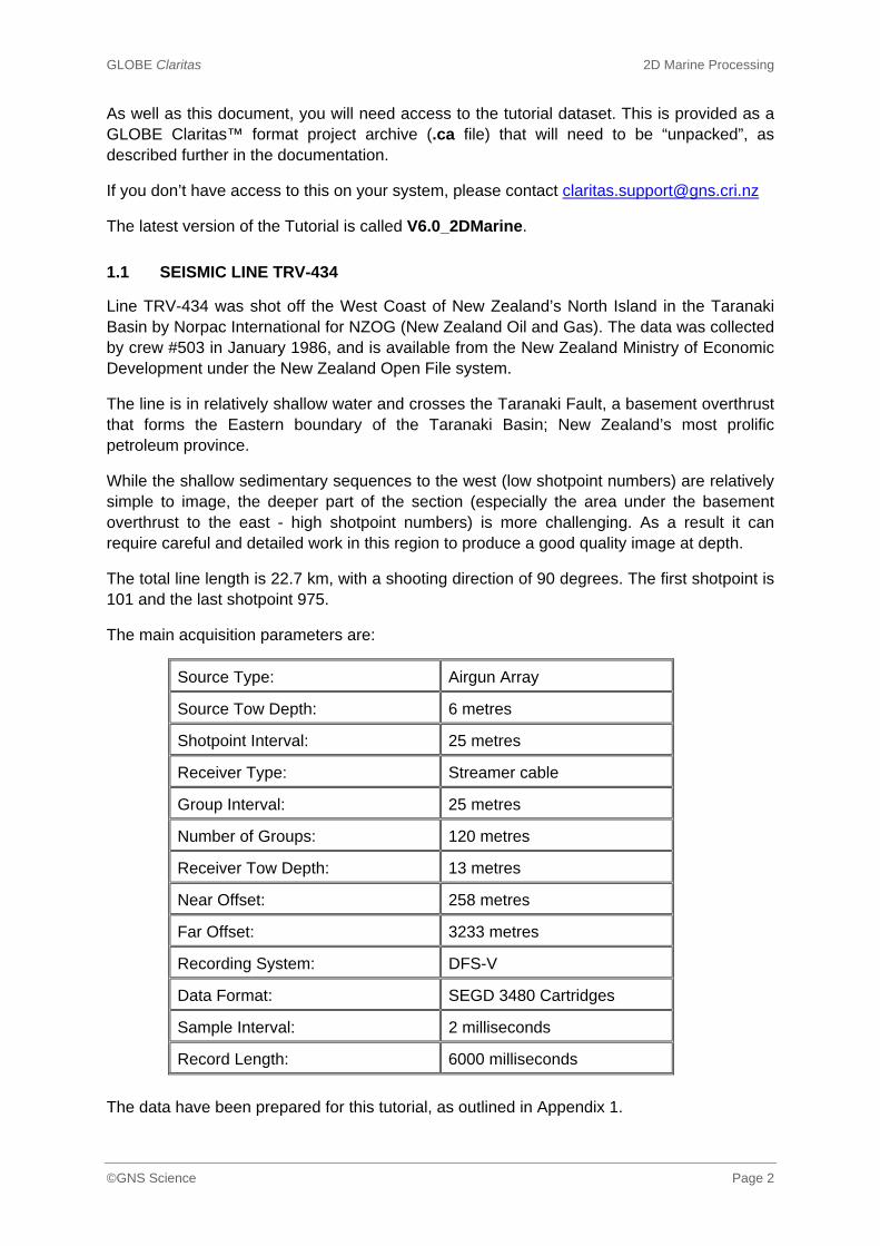
1.1 SEISMIC LINE TRV-434
Line TRV-434 was shot off the West Coast of New Zealand’s North Island in the Taranaki Basin by Norpac International for NZOG (New Zealand Oil and Gas). The data was collected by crew #503 in January 1986, and is available from the New Zealand Ministry of Economic Development under the New Zealand Open File system.
The line is in relatively shallow water and crosses the Taranaki Fault, a basement overthrust that forms the Eastern boundary of the Taranaki Basin; New Zealand’s most prolific petroleum province.
While the shallow sedimentary sequences to the west (low shotpoint numbers) are relatively simple to image, the deeper part of the section (especially the area under the basement overthrust to the east - high shotpoint numbers) is more challenging. As a result it can require careful and detailed work in this region to produce a good quality image at depth.
The total line length is 22.7 km, with a shooting direction of 90 degrees. The first shotpoint is 101 and the last shotpoint 975.
The main acquisition parameters are:
Source Type: Airgun Array
Source Tow Depth: 6 metres
Shotpoint Interval: 25 metres
Receiver Type: Streamer cable
Group Interval: 25 metres
Number of Groups: 120 metres
Receiver Tow Depth: 13 metres
Near Offset: 258 metres
Far Offset: 3233 metres
Recording System: DFS-V
Data Format: SEGD 3480 Cartridges
Sample Interval: 2 milliseconds
Record Length: 6000 milliseconds
The data have been prepared for this tutorial, as outlined in Appendix 1.

GLOBE Claritas 2D Marine Processing
©GNS Science Page 3
2. GETTING STARTED WITH GLOBE CLARITAS
2.1 OBJECTIVES
• Familiarity with the GLOBE Claritas Launcher.
• Getting help
• Introduction to GLOBE Claritas projects.
• Archiving and Recovering Projects.
2.2 THE GLOBE CLARITAS LAUNCHER
The GLOBE Claritas Launcher gives access to all the GLOBE Claritas applications and utilities, grouped into broad classifications. It allows easy access to all of the tools and utilities and is fully integrated with the project-based data management layer (DML). On the Windows operating system you can start the Launcher by clicking on the GLOBE Claritas™ icon on the desktop; on Linux simply type ‘launcher’ at the prompt in a terminal window.
The Launcher tabs (down the right side) allow you to select the different classifications of application or utility. In some cases the same application may be under several classifications but operating in different modes.
The GLOBE Claritas Launcher

GLOBE Claritas 2D Marine Processing
©GNS Science Page 4
In Linux, if you would prefer a “horizontal” layout of the tabs, you can start the Launcher in this mode by typing ‘launcher –h’. Using the Launcher is strongly encouraged, however all of the utilities and applications it is used to access can also be run directly from a terminal prompt. Once the GLOBE Claritas™ environment has been started, simply type the command name. The Launcher can work in two ways; using the menus at the top you can either (1) specify a working directory or (2) select a project to work in. Any application you open is labelled with the project it was started under and/or the local directory and you can change either at any time.
2.3 GETTING HELP
One of the key category tabs to be aware of is the Help area; this allows access to the full on-line help utility and if you are connected to the internet, the on-line bug-reporting system. From Version 6.0 onwards the manual and support information is provided in web browser format; clicking on the buttons on the launcher will automatically start your default web browser and point to the introduction web pages (illustrated below).
The GLOBE Claritas manual in web-browser based form

GLOBE Claritas 2D Marine Processing
©GNS Science Page 5
The web browser based manual has links to online support information from: the GLOBE Claritas™ forum, LinkedIn Group and YouTube channel. Version 6.0 still allows you to access the older text-based application ‘Seishelp’, which may be useful for smaller display screens or if resources are limited. This can also be started by typing “seishelp” at a terminal prompt.
The initial selection menu displayed by running the Seishelp utility
These systems are parallel, and generated from the same source data. While you can generally access the same information directly from within all of the applications and utilities, the search functionality can be very useful when trying to develop workflows or resolve specific processing issues. More detailed descriptions of the modules, applications and utilities used in the tutorial can be accessed from the Manual at any time.
2.4 GLOBE CLARITAS PROJECTS
GLOBE Claritas™ uses a fixed directory structure to store the files associated with each project. These files might be seismic data, navigation information, workflows or supporting text files. The use of projects is optional but, in conjunction with the GLOBE Claritas™ Launcher, greatly simplifies the data management aspects of seismic processing. NB: there is no underpinning database – the user can still locate and interact with data and support information without “exporting” them from the project.

GLOBE Claritas 2D Marine Processing
©GNS Science Page 6
While the file structure and naming conventions are fixed, the user can specify the directory (or folder) for the main project structure. Users also have the option to specify a different directory (or folder) for the data storage - output data files often require far more disk space than processing flows or support files.
If you click on the ‘Project’ menu at the top of the Launcher (as opposed to the ‘Projects’ tab on the right-hand menu) you can select from a list of projects that are configured on your system.
If you are working with a fresh installation of GLOBE Claritas™ this may be blank!
A central repository is used to hold basic information on all the projects that are available; this may be local to your workstation or shared on a multi-user system.
The various utilities for managing projects can be found under the ‘Projects’ tab – here you can create, edit, remove, register, archive, and restore projects.
Selection choices available under the Projects tab in the Launcher
You would normally start off by creating a new project, but in this case we will be restoring from an archived project.
In both cases you will be prompted for a project directory; this is the directory path (or folder) where you want to store all of your projects and should exclude the name of the project itself since this is generated automatically.

GLOBE Claritas 2D Marine Processing
©GNS Science Page 7
Click on the ‘Restore’ button and complete the form. Select an appropriate location on your system for the project to be stored; you can give the project a unique name but should specify the full path to the archive file <NAME>. You can search for this using the ‘List’ button.
A project can be archived at any time thus allowing full or partial backups. A partial backup excludes the data directories and so is much smaller in size.
NB: using the Archive function followed by the Restore function is the only way to rename a project or change the directories being used.
When you restart the Launcher, GLOBE Claritas™ will automatically select the most recently used project. You can change the active project by clicking on ‘Project’ at the top of the Launcher and selecting from the drop-down list.
The directory structure for a GLOBE Claritas project (Windows 7); the project name is
MARINE2D_V6, below this is the COMMON directory and then directories for each of the main
data and file types. This is created and populated automatically by the project restore process
Expert User Tips:
‐ Use the “Shared Registry” option to create a list of projects that is not stored in the
GLOBE Claritas installation directory; this could be on a networked drive, for example
‐ If you start working without first creating a project, you can use the Import option to
create a project. Files are automatically imported to their “correct” locations by type
‐ GLOBE Claritas™ applications will automatically search in the correct directory for files of a
given type, but you can always manually specify a different pathname or file type

GLOBE Claritas 2D Marine Processing
©GNS Science Page 8
3. INITIAL DATA QC USING XSJE AND XVIEW
3.1 OBJECTIVES
• Familiarity with the XSJE job flow editor.
• Adding, parameterising, activating and deactivating modules in the job flow editor.
• Reading in selections from a larger dataset.
• Running GLOBE Claritas™ jobs.
• The XVIEW interactive seismic display.
• Adjusting XVIEW display scales and appearance.
• XVIEW Seismic Data Analysis and Zoom Windows.
• XVIEW Amplitude Histogram Window.
• Adjusting XVIEW seismic display colours.
• QC of raw seismic shots, refraction energy and the effects of AGC.
3.2 XSJE: THE SEISMIC PROCESSING JOB FLOW EDITOR
Seismic processing flows in GLOBE Claritas are stored as ASCII files with a .job extension.
A processing flow is made up of a series of processing modules (or processors), usually starting with an input module and having some kind of output - which could be to the screen or to a file.
While you could open and edit a processing flow with a simple text editor, this is extremely difficult in practice. The XSJE seismic job editor has been created to make building processing flows as simple as possible.
From the Launcher, click on the ‘Flows’ tab, then on the ‘Job Files’ button and open the file 00_qc.job.
If you expand the window you can see a short text description of what each module is doing; double click on these to edit the text.
Look at the parameterisation of each module by double-clicking on it – this opens a parameter form where you can modify or update all of the parameters associated with the module.
GLOBE Claritas 2D Marine Processing
©GNS Science Page 9
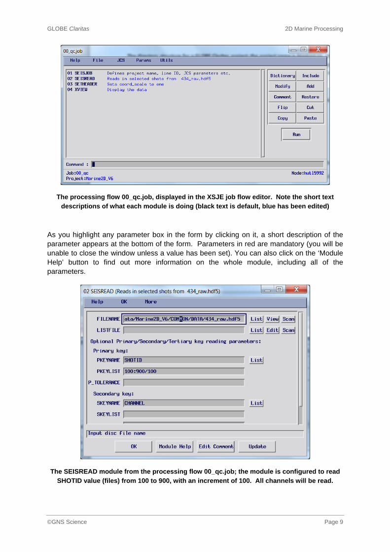
The processing flow 00_qc.job, displayed in the XSJE job flow editor. Note the short text
descriptions of what each module is doing (black text is default, blue has been edited)
As you highlight any parameter box in the form by clicking on it, a short description of the parameter appears at the bottom of the form. Parameters in red are mandatory (you will be unable to close the window unless a value has been set). You can also click on the ‘Module Help’ button to find out more information on the whole module, including all of the parameters.
The SEISREAD module from the processing flow 00_qc.job; the module is configured to read
SHOTID value (files) from 100 to 900, with an increment of 100. All channels will be read.
GLOBE Claritas 2D Marine Processing
©GNS Science Page 10
The job you have opened uses SEISREAD to read in the reformatted and resampled shots, with SHOTID and CHANNEL set as the primary and secondary keys. Only certain shots are selected in the module (from 100 to 900 in increments of 100). This is defined by the PKEYLIST parameter; click on the ‘Module Help’ button for more information on complex selections.
NB: all GLOBE Claritas™ processing flows must start with the SEISJOB module. When you create a new job flow this will be inserted automatically.
The XVIEW module is for interactive display and analysis. It can be used to display either pre-stack or post-stack data. In this case, the module is configured to display 9 ensembles (or groups of data) each with 120 traces – in other words, 9 shots each with 120 channels.
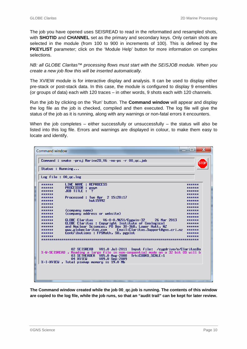
Run the job by clicking on the ‘Run’ button. The Command window will appear and display the log file as the job is checked, compiled and then executed. The log file will give the status of the job as it is running, along with any warnings or non-fatal errors it encounters.
When the job completes – either successfully or unsuccessfully – the status will also be listed into this log file. Errors and warnings are displayed in colour, to make them easy to locate and identify.
The Command window created while the job 00_qc.job is running. The contents of this window
are copied to the log file, while the job runs, so that an “audit trail” can be kept for later review.

GLOBE Claritas 2D Marine Processing
©GNS Science Page 11
When you run the job, the XVIEW window will appear within a few seconds and a grey vertical progress bar (on the left hand side) will indicate how much of the data has loaded. After enough data has been collated to fill the display, a green bar will show the progress in rendering the display. On most systems this will happen almost too fast to see, but if you have a lot of modules in the flow or a slow display speed from a remote location, you may see both the grey and green coloured bars.
The data will start to display, but you will need to use the scroll bars to see it all. Note that once the data has all been loaded for display, the cursor changes shape to a cross.
The XVIEW display generated by 00_qc.job. The display is fully interactive and can be used to
analyse data in a number of different ways. The first four (of nine) selected shots is displayed here
Geophysics Comments:
‐ Look at the shots; they are dominated by linear direct arrivals and refraction energy in
terms of amplitudes, but you can still see some hyperbolic reflections in the gathers,
especially in the shallow part of the data (under two seconds)
‐ On SHOTID 200 there is a significant low frequency “sea swell” noise burst between
channels 36 and 42, which will need to be addressed
‐ You can also see “tail buoy jerk” on SHOTID 400, especially above the seismic data; it is
caused by the end of the cable being moved about by the swell. This sets up pressure
waves in the cables, which are oil‐filled for neutral buoyancy. “Tail buoy jerk” is low
frequency and dips from “tail to head” on the cable.
GLOBE Claritas 2D Marine Processing
©GNS Science Page 12
As you move the cursor around, the trace amplitude, primary key and the time in milliseconds are displayed in the top left corner.
The data is not very well scaled at the moment. One way to resolve this is to apply an AGC (automatic gain control) to the data. You can do this interactively by clicking on the “Process” button in the top left corner of the window.
This allows you to enter a short processing sequence to be applied; in this case enter the word “AGC” and press return when prompted. Use the default parameter values for now.
You can toggle the effect of the AGC on and off by clicking the Process button.
Click on the ‘Next’ button – since there is no more data to display, the job completes. If there were more than 9 shots to be viewed the ‘Next’ button would display the next 9 shots, and so forth.
Clicking on ‘Close’ from the menu at the top of the display window will complete the job and shut down the display. You will be left with only the Command window; click the ‘Dismiss’ button to close it.
You can also terminate a job by clicking the red ‘Stop’ button in the Command Window.
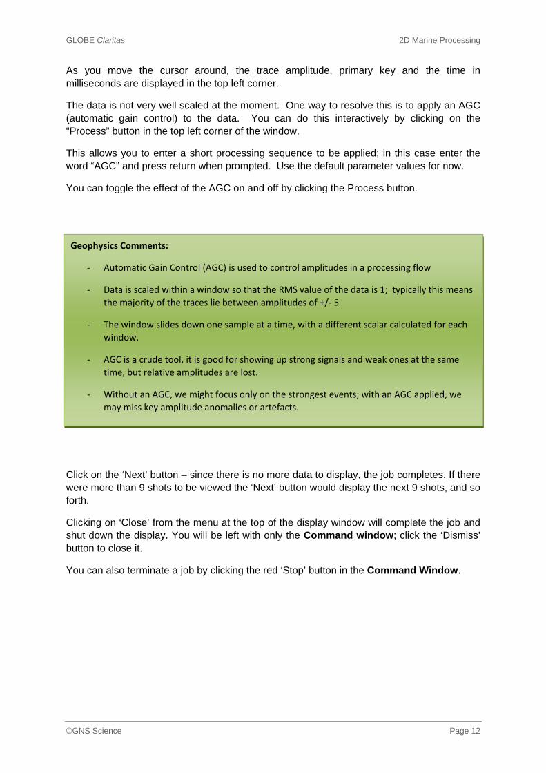
Geophysics Comments:
‐ Automatic Gain Control (AGC) is used to control amplitudes in a processing flow
‐ Data is scaled within a window so that the RMS value of the data is 1; typically this means
the majority of the traces lie between amplitudes of +/‐ 5
‐ The window slides down one sample at a time, with a different scalar calculated for each
window.
‐ AGC is a crude tool, it is good for showing up strong signals and weak ones at the same
time, but relative amplitudes are lost.
‐ Without an AGC, we might focus only on the strongest events; with an AGC applied, we
may miss key amplitude anomalies or artefacts.

GLOBE Claritas 2D Marine Processing
©GNS Science Page 13
3.3 ADDING, DELETING AND FLIPPING MODULES
You can also add an AGC module into the processing flow. To do this
‐ On the XSJE editor, click on the ADD button
‐ Click on “Alphabetic Listing” and click OK
‐ Select AGC from the list and click OK
‐ The pointer will change shape
‐ Position the pointer between module 03 (SETHEADER) and 04 (XVIEW) and click
‐ The module will be inserted, and you can modify the parameters as before
Run the job to confirm that AGC has had the desired effect.
Now highlight the AGC module and then click the ‘Flip’ button to deactivate it.
The processing flow 00_qc.job with the module AGC added and then “Flipped” to deactivate it
Expert User Tips:
‐ You can double‐click to avoid having to click ‘OK’ after each step above.
‐ You can also insert a module using the keyboard by typing commands.
‐ In the ‘Command’ field, type “add AGC 04” and press enter to add the AGC module
between the SETHEADER and XVIEW modules.
‐ Use append or app to add a module to the end of the flow; app AGC.
‐ If you just type app or add this opens a selection dialogue, exactly as if you had pressed
the buttons.

GLOBE Claritas 2D Marine Processing
©GNS Science Page 14
Re-run the job and you will see that the AGC is no longer applied to the flow. When a module is selected you can use the right mouse button to bring up a menu list of options including ‘Flip’.
This is very useful in checking flows, finding out why they are not working as expected or quickly reviewing alternative sequences.
You can experiment further by adding in the BALANCE module; the default mode for this module uses a single gate to compute a single scalar for the whole trace to a reasonable level, as opposed the sliding window used in AGC.
Multiple modules can be highlighted by dragging over them with the left mouse button; you can then ‘Cut’ or ‘Copy’ and ‘Paste’ part of a sequence. You can also include modules from other processing flows, using the ‘Include’ button.
3.4 CONFIGURING DIFFERENT DISPLAY MODES
You can modify the display parameters directly in the XVIEW module before the job has run, or in the XVIEW display while it is running; click on ‘Params’ and select ‘Main Plot’.
The Display mode field (which can also be accessed directly from the XVIEW display window by clicking on ‘Plotmode’) allows you to explore different display types: variable density (VD), variable area wiggle (VAWG), variable area (VA) and wiggle (WG).
In VD mode, a horizontal colour bar appears at the bottom showing how the amplitudes are mapped to colours in the display. Clicking on the colour bar will cycle through different pre-defined colour maps; right click to select from a list.
Expert User Tips:
‐ To look at the files created while we have been working, open a terminal window from the
Launcher by clicking on the ‘Terminal’ button on the ‘Flows’ tab.
‐ Here you can enter UNIX/Linux commands – even if you are running GLOBE Claritas™
under Windows. If you type “ls ‐latr 00_qc.*”, you will see a complete list of all of the files
associated with running this job. The .job file contains the workflow, and the .log file is the
log output from the Command window.
‐ Note that each time you run a job, the log file will have the same name, even if you have
added modules or changed parameters. The current log file is called 00_qc.log; if the job is
re‐run a new log is created and the old version is renamed to 00_qc.log~. When running a
testing sequence it is a good idea to save each job under a different name as you edit or
change the flow, using the “File: Save As” option. This avoids losing old tests and
examples.
GLOBE Claritas 2D Marine Processing
©GNS Science Page 15
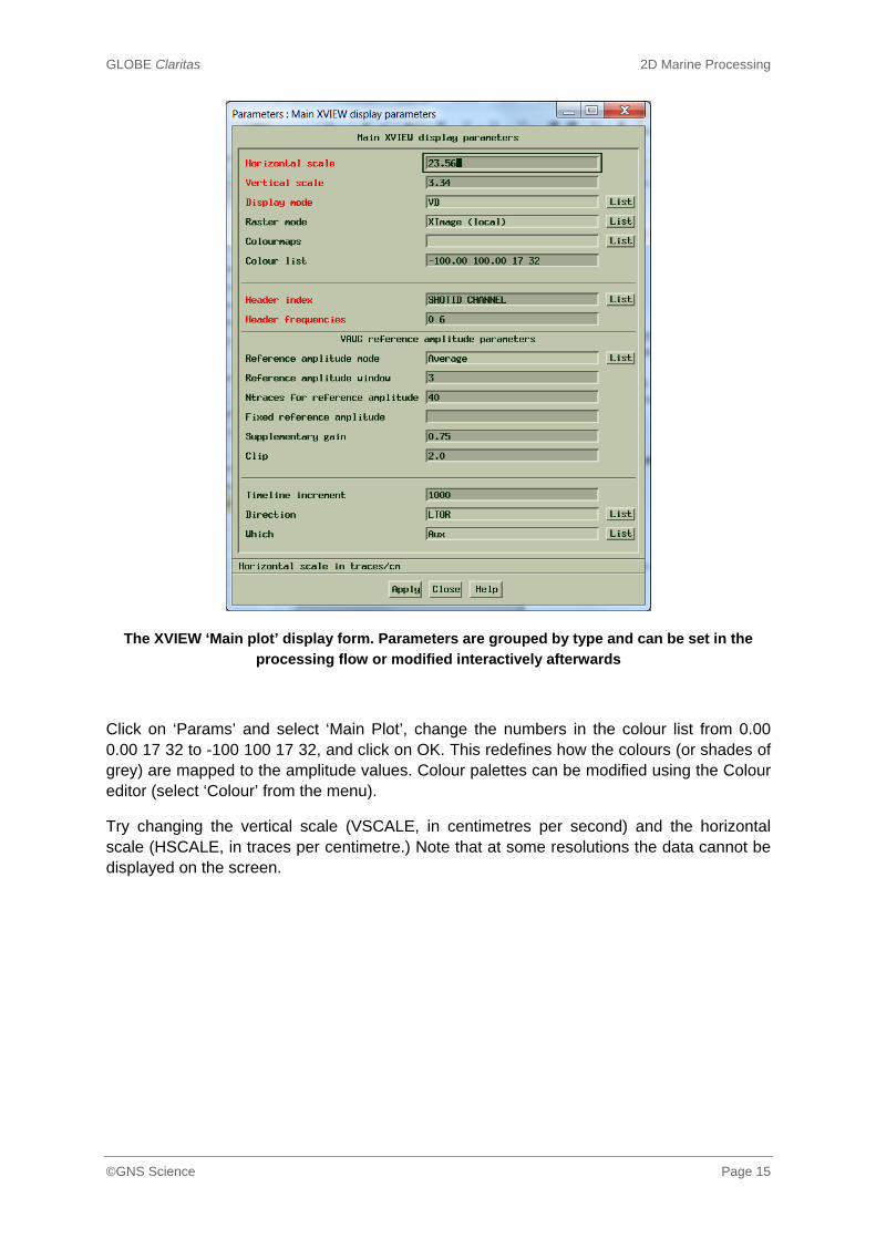
The XVIEW ‘Main plot’ display form. Parameters are grouped by type and can be set in the
processing flow or modified interactively afterwards
Click on ‘Params’ and select ‘Main Plot’, change the numbers in the colour list from 0.00 0.00 17 32 to -100 100 17 32, and click on OK. This redefines how the colours (or shades of grey) are mapped to the amplitude values. Colour palettes can be modified using the Colour editor (select ‘Colour’ from the menu).
Try changing the vertical scale (VSCALE, in centimetres per second) and the horizontal scale (HSCALE, in traces per centimetre.) Note that at some resolutions the data cannot be displayed on the screen.

GLOBE Claritas 2D Marine Processing
©GNS Science Page 16
3.5 INITIAL DATA QC: XVIEW ANALYSIS AND ZOOM WINDOWS
Re-run the job, making sure the AGC module is “flipped” off (and BALANCE has been removed).
At the bottom of the XVIEW window is an ‘Analysis’ button; you can select an option to active a particular analysis window (e.g. FK spectrum), and then highlight an area on the main data window by dragging with the left mouse button. A new window is created with the analysis results.
NB: right-click (and hold) in the display window will also bring up the list of Analysis options
The first option, ‘Seismic Data Zoom’, simply selects a range of data and displays it at a different scale; this window can be saved as a separate SEGY file, which can be handy for creating a small subset of data.
The other zoom windows can be used to look at the trace amplitude, frequency content and to perform transforms on the selected data range.
If you want any of the analysis zoom windows to apply to a whole ensemble of data (in this case a shot), you simply have to click the left mouse button once on the target shot, rather than defining a zoom window.
To change the parameters used to define a zoom window, select ‘Params’ and ‘Seismic data zoom’ from the menu (or press ‘Alt-P’ then ‘d’).
Expert User Tips:
‐ the + ‐ and < > keyboard keys can be used to quickly adjust the plot scale
‐ the +/‐ buttons at the top left of the display can be used to change the plot gain
‐ Alt‐P followed by m will open the Main Plot parameter form
‐ Hold Ctrl and use the scroll wheel to zoom in or out
‐ Hold the middle mouse button to “pan” the display without using the scroll bars
‐ Specifying 30.0 on the horizontal display will force a scale of 30 traces per centimetre.
‐ Specifying 30 on the horizontal display will give you the closest value to this that does not
“hide” or “alias” the traces based on your screen resolution

GLOBE Claritas 2D Marine Processing
©GNS Science Page 17
As an example exercise to recap what we have looked at:
Change the main display parameters to variable density using the options on the ‘Main plot’ parameters form, and click on ‘Apply’.
Use the ‘Amplitude Histogram’ analysis window to look at the range of sample amplitude values.
Click on the ‘Process’ button, and apply a 500ms AGC.
Open the ‘Amplitude Histogram’ analysis window again, and see how the histogram has changed.
Open the ‘Main plot’ parameter form and adjust the Colour list parameter to make better use of the available colour range, given the modified amplitudes
Open the ‘Amplitude Histogram’ analysis window again and see how the histogram has changed.
The other zoom windows work in essentially the same way, and allow for a range of interactive analysis.
When you have finished, close the XVIEW window, dismiss the Command window, and exit XSJE by selecting ‘File’ and ‘Save & Exit’.
4. SHOT-BASED PRE-PROCESSING AND NOISE SUPPRESSION
4.1 OBJECTIVES
Picking refraction mutes in SV.
The XSDE support/control file editor and file formats.
Amplitude recovery tests.
Using the REPEAT functions for testing with IF/ENDIF.
Manipulating trace headers using HEADER and SETHEADER.
Spatially varying support files (SCALE) and use with REPEAT.
Multi-panel displays in XVIEW for testing.
Labelling panels in XVIEW.
XVIEW Amplitude Decay Zoom Window.
XVIEW Frequency Spectra Zoom Window.
XVIEW linear and hyperbolic velocity rulers.
GLOBE Claritas 2D Marine Processing
©GNS Science Page 18
Testing swell-noise suppression filters.
XVIEW "difference" panels.
FK-Filters and detecting spikes.
Spike detection and editing using the Areal application and module.
Use of SLI to interrogate and investigate seismic files.
Building a production job from tests.
Basic QC steps.
Reading multiple seismic files in a job flow.
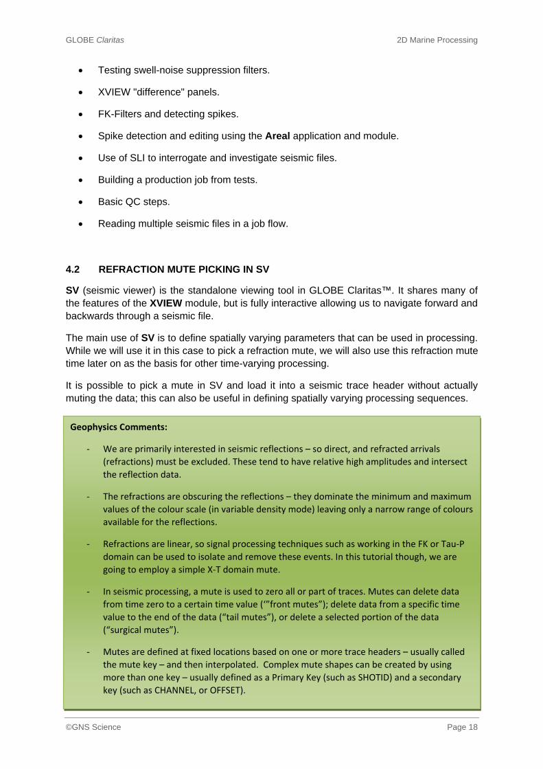
4.2 REFRACTION MUTE PICKING IN SV
SV (seismic viewer) is the standalone viewing tool in GLOBE Claritas™. It shares many of the features of the XVIEW module, but is fully interactive allowing us to navigate forward and backwards through a seismic file.
The main use of SV is to define spatially varying parameters that can be used in processing. While we will use it in this case to pick a refraction mute, we will also use this refraction mute time later on as the basis for other time-varying processing.
It is possible to pick a mute in SV and load it into a seismic trace header without actually muting the data; this can also be useful in defining spatially varying processing sequences.
.
Launch the SV application (under the ‘Seismic Data’ tab on the Launcher) and use the ‘List’ button to select the file 434_raw.hdf5
Geophysics Comments:
‐ We are primarily interested in seismic reflections – so direct, and refracted arrivals
(refractions) must be excluded. These tend to have relative high amplitudes and intersect
the reflection data.
‐ The refractions are obscuring the reflections – they dominate the minimum and maximum
values of the colour scale (in variable density mode) leaving only a narrow range of colours
available for the reflections.
‐ Refractions are linear, so signal processing techniques such as working in the FK or Tau‐P
domain can be used to isolate and remove these events. In this tutorial though, we are
going to employ a simple X‐T domain mute.
‐ In seismic processing, a mute is used to zero all or part of traces. Mutes can delete data
from time zero to a certain time value (‘”front mutes”); delete data from a specific time
value to the end of the data (“tail mutes”), or delete a selected portion of the data
(“surgical mutes”).
‐ Mutes are defined at fixed locations based on one or more trace headers – usually called
the mute key – and then interpolated. Complex mute shapes can be created by using
more than one key – usually defined as a Primary Key (such as SHOTID) and a secondary
key (such as CHANNEL, or OFFSET).

GLOBE Claritas 2D Marine Processing
©GNS Science Page 19
When prompted, type “refraction” in the Output files parameter; this will form part of the name of the file that is created. Ensure that the Time range parameter is “0 3000”; 0ms to 3000ms.
A message will pop up describing that the data does not have an appropriate coordinate scalar set.
This is not surprising as there is no geometry information (spatial coordinates) in the data yet, on which to apply a scalar; we will add this further along in the processing. For now, tick the “Do not display this warning again” box, and click ‘Continue’.
SV being used to pick a refraction mute; the squares are the “knee points”, with the
red-highlighted point showing it is active as the pointer is nearby

GLOBE Claritas 2D Marine Processing
©GNS Science Page 20
SV uses the same display components and controls as XVIEW; the main difference is that with SV we can step forwards and backwards through a dataset, using the arrow buttons at the top of the display window. You can also skip to any location by clicking on the primary key name (SHOTID in this case) and entering a value into the Ensemble to jump to field on the window that pops up. The primary key range is also displayed, at the bottom of the window.
You can control how many ensembles (in this case shot records) are displayed, as well as the “step” increments used by the single and double headed arrow “skip” buttons.
SV also includes tools for picking and analysis; first break, mutes, and horizons can all be picked. To keep the interface simple, you can choose which families of buttons (or toolbars) to display – click on the ‘Toolbar’ button to see the list.
Select ‘Add Muting Buttons’ to add the controls needed to create a mute; you can then click on the ‘FrontMute’ button. Check that Offset extrapolation mode is set to ‘Sloped’ and the Secondary key name is set to ‘CHANNEL’.
To pick a mute in SV, first click on the ‘FrontMute’ button to enter picking mode. Picking is with the left mouse button – one click adds a pick and a second one removes it. To move a pick, hold the left mouse button down when the pick is active (red). Each left mouse button click adds a knee-point in the mute line. The thin blue line shows how the mute will be extrapolated away from your current picks, and when you move to another location, how the mute is currently interpolated.
In this case, with a front mute, everything above the mute line will be rejected. Aim to cut out almost all of the (linear) refraction data at the start of the shot. Note the sloped interpolation mode means you don’t have to make picks at the start or end of the data.
Once you have finished, click on ‘File’ and ‘Exit’; the mute is automatically given the correct three letter file extension (.smu) and saved into the correct project directory (../COMMON/MUTES).
Geophysics Comments:
Refraction mute picking tips:
‐ Pick from the high CHANNEL (near offset) to the low CHANNEL.
‐ Leave the first few traces with unmuted to ensure the seabed reflection is retained.
‐ Aim to remove almost all of the refraction energy finishing at about 2600ms on
CHANNEL=1.
‐ The water depth on this line is pretty constant however the near surface geology
changes quite a lot so you may want to vary the mute along the line.

GLOBE Claritas 2D Marine Processing
©GNS Science Page 21
4.2.1 Parameter Files: The XSDE Editor
To look at the mute file you have created (it will be called refraction.smu) use the seismic data editor (XSDE). From the ‘Flows’ tab, click the ‘Control files’ button. If you didn’t pick your own mute you can look at the predefined file GNS_refraction.smu in the ../COMMON/MUTES directory.
Although you can edit GLOBE Claritas™ support files directly (by clicking on the ‘Text files’ button under the ‘Flows’ tab), XSDE uses a spread sheet format for simpler data entry. For mutes, the file contains a list of the time/channel pairs that you have selected. To exit, select ‘File’ and ‘Quit xsde’.
The picked refraction mute file displayed in the XSDE editor. Users can add, delete or edit
values as well as apply mathematical functions to columns if needed
Expert User Tips:
‐ Adding in the trace editing toolbar allows options to kill any noisy traces. The edits file will
have the correct extension added automatically and be saved into the correct directory.
‐ You can also pick the mute based on offset instead of channel, if you prefer.
‐ Select ‘File’ then ‘Load input file’ to import an existing mute file (.smu) for QC or editing of
the picks that have been made.
‐ You can apply NMO to the data, using the process button, allowing you to pick NMO
stretch mutes if desired.

GLOBE Claritas 2D Marine Processing
©GNS Science Page 22
4.2.2 Checking the Mute Application: REPEAT Panels, IF and ENDIF
Now we need to test-apply the mute to make sure it does what we want. Open the job 01_mutes.job by clicking on the Job Flows button.
This flow uses some of the additional functionality in the SEISREAD module, designed to help testing and QC. The module populates a special trace header (called REPEAT) with a counter, and creates a duplicate copy of the data. This counter shows which copy number of the data the trace belongs to. You can repeat the dataset as many times as you want.
In a processing flow, you can make selections based on trace headers using the IF module. The IF module acts as a branch in the processing sequence through which some of the data can be sent. The ENDIF module marks where the branch re-joins the main processing sequence. In this job, the SMUTE module (to apply the refraction mute) is only used when REPEAT=2 in the IF module parameters.
The 01_mutes.job processing flow, using IF/ENDIF as well as duplicates of the data
Open up the SEISREAD and IF modules before running the flow to make sure you understand how these are being parameterised; this type of “panel test” is fundamental to how we use GLOBE Claritas™ for checking and QC’ing data.

GLOBE Claritas 2D Marine Processing
©GNS Science Page 23
The SEISREAD module, with the NREPEAT
parameter set to create two copies of the data
The IF module configured to select data
where the REPEAT header is set to 2. You
can create complex selections using
RANGE, GROUP as well as lists of trace
header values
When you run the job, two sets of seismic data are displayed, corresponding to each value of REPEAT that has been set. The first panel (REPEAT=1) shows the original data while the second panel (REPEAT=2) displays the muted data.
XVIEW display with REPEAT panels; the numbered boxes (lower left corner) show the REPEAT
value. Use the mouse, arrow keys or number keys to toggle
GLOBE Claritas 2D Marine Processing
©GNS Science Page 24
4.3 AMPLITUDE RECOVERY TESTS WITH REPEAT
The seismic wave front loses energy as it propagates through the Earth. This is a result of absorption, transmission/reflection losses, and the fact that it is spreading out spherically. We can attempt to compensate for this loss of energy by applying a time- and space-variant gain to the raw seismic shots.
The processing flow 02_TAR.job demonstrates a more sophisticated testing sequence using the REPEAT and IF options, and creates six different test panels.
The processing flow also applies a simple marine geometry to the data which assumes the cable follows in a straight line behind the boat; this is in order to populate the source-receiver distance (OFFSET).
Open the processing flow 02_TAR.job using the XSJE job flow editor and step through the modules, looking at how the selections have been made.
The MGEOM module is used to define the acquisition geometry – it uses a special parameter file that is created using the ‘Marine’ button under the ‘Geometry’ tab on the Launcher. You can access this file directly from the MGEOM module by clicking the ‘Edit’ button.
Expert User Tips:
‐ You can have as many repeat panels as you like; the number keys allow you to toggle
easily between REPEAT values in the XVIEW display.
‐ IF loops can be part of a more complex sequence, with ELSEIF and IFNOT modules, if
required.
Geophysics Comments:
‐ True Amplitude Recovery (TAR) involves correcting for the reduction in seismic amplitudes
over time; the signals we receive first are stronger than those we receive later. The
majority of the reduction occurs because of the spherical spreading of the wavefield as it
propagates – the same amount of energy is spread over a larger area. Additional losses
are caused partially through scattering and inelastic responses, but also from mode
conversion (creation of refractions, S‐waves and so on) at layer boundaries.
‐ We usually apply corrections for these losses in two stages. The first is a ‘spherical
divergence’ correction, usually expressed as a function. This function is a power of: two
way time (T), and/or the sub‐surface velocity (V), e.g. T2V. The second stage is applied as a
linear gain, in decibels and two‐way‐time (1dB/second, 2dB/second and so on).

GLOBE Claritas 2D Marine Processing
©GNS Science Page 25
The marine geometry form, configured for line TRV-434. The CDP spacing is usually half of the
group interval; note that (as we have seen) the far channel from the boat is 120, not 1

GLOBE Claritas 2D Marine Processing
©GNS Science Page 26
The MGEOM module will assign or use the following headers; you can change some of these in the form, but we recommend you start with these defaults. The mandatory headers should not be redefined, as they are used elsewhere in GLOBE Claritas™.
Header name Usage
Mandatory
name?
RECORDNUM
The file numbers as recorded on tape; on older data this
may loop to zero at 99 or 9999 NO
SHOTID
The renumbered file numbers, updated to match the FFID
numbers in the observer’s logs; may be the same as
RECORDNUM
YES
SOURCENUM
The shot point number as referenced in the navigation and
observer’s logs; may be the same as the FFID (SHOTID) or
need remapping
NO
SPARE4
The position of a given CDP, expressed as a shot point
number; created by MGEOM YES
CDP
The common depth point (midpoint number), created by
MGEOM NO
CDPTRACE The trace number within a CDP gather, created by MGEOM NO
REC_PEG
The common receiver location for the data, to enable sorting
to receiver gathers, created by MGEOM NO
OFFSET
The distance from the source to the receiver. Created by
MGEOM NO
COORD_SCALE
Defines the units (metres, decimetres) used for OFFSET.
Created by MGEOM NO
CDP_X and CDP_Y
SOURCE_X and
SOURCE_Y
REC_X and REC_Y
X, Y co-ordinates of the CDP, shotpoint and receiver,
relative to the start of the line. Created by MGEOM NO
It is possible to renumber the SHOTID values, allowing for any missing files using the RENUMBER module. Similarly you can renumber the SOURCENUM values to allow for any missing shot points (due to vessel speed for example). SPARE4 is automatically allocated by the MGEOM module.
Each of the repeated shots will have different types of scaling applied after the refraction mute. IF/ENDIF pairs are used to make these selections. REPEATS 2 and 6 have a spherical divergence correction applied. Note that the velocity file used by the spherical divergence module has a similar name to the job, for clear identification.

GLOBE Claritas 2D Marine Processing
©GNS Science Page 27
The job flow 02_TAR.job, which applies different amplitude corrections and presents the
results as a series of test panels for the user to review
We could have individually selected REPEATS and applied different gains to them one at a time, but it is far easier to use the IF module to select a range of repeat values (from 3 to 6) and apply different gains from a single scalar support file.
The SCALE module, and associated .scl parameter file
The SCALE module can vary with a primary key, and in this case we have used REPEAT. Each of the values of REPEAT has its own scalar function defined. You can view (or edit) the support file by clicking on the ‘Edit’ button.
When you first set up a GLOBE Claritas™ job, selecting the ‘Edit’ button can also be used to create new support files, without needing to exit the job flow editor.

GLOBE Claritas 2D Marine Processing
©GNS Science Page 28
Finally, the BALANCE will ensure we can view all of the data at the same scale, and compare the relative change in amplitudes within each test panel. The PANELTEXT module labels each of the tests displayed in XVIEW with a text header.
Run the job.
Each of the REPEAT values appears in a different panel in XVIEW, numbered along the bottom from 1 to 6. This enables rapid visual comparison of the test results. You can scroll through the panels using the arrow keys, the mouse, or by using the number keys on the keyboard.
For a more quantitative analysis, click on the ‘Analysis’ button and select ‘Amplitude Decay Curve’.
A single left-click on the shot record brings up an amplitude decay curve for the whole shot.
Click ‘AllPanels’ from the menu in the zoom window, and an amplitude decay curve for each repeat panel is created. You can then click ‘SyncPanels’ so that panels on both the seismic display and the zoom window are synchronised.
The amplitude decay curve analysis window, showing how well spherical divergence alone
corrects for the amplitude decay on these data
Make a note of your preferred amplitude recovery approach in your Testing Log.

GLOBE Claritas 2D Marine Processing
©GNS Science Page 29
4.4 SWELL NOISE ANALYSIS AND SUPPRESSION TESTS, DIFFERENCE PLOTS
Now that the amplitudes in the traces are well balanced, we can start to address some of the noise. The low frequency noise bursts clearly visible in the data are a result of the sea-swell and need to be removed.
Run the job 03_swell.job which applies both the refraction mute and amplitude recovery before displaying the data. This job uses the REPEAT processing module in place of the options to set the REPEAT header in SEISREAD for testing.
The processing flow 03_swell.job; this flow uses the REPEAT module, in place of the REPEAT
options in SEISREAD
When you run the processing flow, the second panel shows the impact of applying a 5Hz-10Hz low-cut filter to remove the swell noise. It is important to look at what this filter is really doing to the data. To do this, click on ‘Utils’, select ‘Plot Difference’, and then click ‘OK’ on the next form.
A third panel will be created that shows the difference between the filtered and the unfiltered section. In this panel you can clearly see what is being removed.

GLOBE Claritas 2D Marine Processing
©GNS Science Page 30
The difference plot between the filtered and unfiltered section, showing how low frequency
signal is also being removed from the data
You can also use the Frequency spectra (traces) analysis window to look at how the frequency content has been modified. Right-click on the display, choose Frequency spectra (traces) and use the left mouse button to draw a box around one of the noise bursts on the first (unfiltered) panel.
Now that we have assigned offsets to the data, we can also use the Ruler to measure the apparent velocity of events. Click on the ‘Ruler’ button, and then use the left mouse button to select the start and end of a straight-line segment. This can be used to help identify other noise trains, as well as to design FK filter dip limits. If you use the middle mouse button to activate the ruler, rather than measuring linear velocity, the ruler shape becomes a hyperbola and measures the NMO velocity.
Expert User Tips:
‐ You can modify the filter parameters in the processing flow, or add more REPEATS and use
IF/ENDIF more than once, to test different parameters. You can also work interactively
using the unfiltered section (panel 1) and the ‘Process’ button to test different filters – the
FDFILT module can be applied interactively.
‐ Effective swell noise suppression can also be achieved by: (1) using the DUSWELL module
and (2) carefully designing an FK domain mute to target the high wavenumber, low
frequency parts of the FK spectrum. You can pick FK domain mutes from the FK spectrum
analysis window, and apply them from a module using the FKMUTE module.
GLOBE Claritas 2D Marine Processing
©GNS Science Page 31
4.5 APPLICATION OF FK FILTERS, DETECTING SPIKES AND MANAGING AMPLITUDES
The processing flow 04_FK.job applies an FK filter that rejects data with a dip of greater than +15ms/ trace (corresponding to rejecting data with an apparent velocity of 1666 m/s or less, given 25 m trace spacing). This is targeting steeply dipping noise that can be seen on the higher shot numbers.
When you run the job, the (introduced!) high amplitude spike in one of the shot records demonstrates the edge effects that can happen with large amplitude variations.
The third panel has a removable AGC “wrapped” around the FK filter, which normalises the amplitude values before the FK filter is applied. The scalar values for each AGC time gate are stored as a “pseudo trace” (created by the AGC module) and then removed by the UNAGC module.
Geophysics Comments:
‐ The FK domain is a two dimensional Fourier transform that is usually displayed with the
frequency of the data vertically, and the wavenumber (or spatial frequency) horizontally.
‐ Energy that has a constant dip in the X‐T domain (but appears at different times) also
appears at a constant dip in the FK domain. This allows us to remove linear dipping noise
(such as direct and refracted arrivals) from the data without impacting on hyperbolic
reflections.
‐ Dips in the filtering domain are usually expressed in terms of milliseconds‐per‐trace, or
metres/second if offsets are present.
‐ As with many multi‐channel processes, FK filters can have edge effects where there are
very low values (such as zero) and extremely large values. This processing flow shows
ways in which these can be mitigated and the consequences when they are not.
‐ A complete discussion of 2D Fourier Transforms can be found in Section 1.2 of the second
edition of “Seismic Data Analysis” by Oz Yilmaz, published by the SEG.

GLOBE Claritas 2D Marine Processing
©GNS Science Page 32
The 04_FK.job processing flow, showing how a removable AGC can be used to prevent
artefacts where there are spikes or large amplitudes present. The AREAL module is configured
to write the RMS of the live portion of the data, into the GAIN_TYPE trace header
The ZEROMUTE module (in Store mode) stores the time of the first non-zero sample into a trace header i.e. it marks the point at which the actual data starts. This can be useful where the mute is unknown (such as when a percentage stretch mute has been applied or after stack) or when you want to use the start of live data as the start time for a window. The data is then being transformed into the FK domain and in doing so (due to approximations made in the transform stages) some amplitudes are ‘smeared’ into the muted area of the data. The application of filters in the FK (and Tau-p) domain can also worsen the effect of this smearing. Once the filter in the FK domain has been applied, the ZEROMUTE (in Mute mode) mutes the data back to the first non-zero point and removes the smearing that was introduced.
The AREAL module can be used to output headers, samples or other attributes such as the peak or RMS value of a trace. In this case, the RMS value of the trace is being written into a trace header. The calculation of the RMS value is in a time window, and this has been specified as being relative to the DELAY header (using the ADDTIME parameter); this header was populated with the time of the first non-zero sample by ZEROMUTE.
Run the job; note how the spike at shot 500 and channel 65 results in a high amplitude "impulse response" dominating the shot panel. Since the FK-filter is a multi-channel process the impulse response function affects the whole shot.
Now plot the GAIN_TYPE header over the data; click on ‘Utils’, then ‘Overlay trace headers’, and complete the parameter form as below:

GLOBE Claritas 2D Marine Processing
©GNS Science Page 33
The plot header parameter form; the header GAIN_TYPE will be plotted centred around the
1000ms time line on the XVIEW plot
On the first panel, you can clearly identify the “spiked” trace on the header plot graph – and channels that still have significant swell noise can also be identified easily.
The unfiltered panel generated by 04_FK.job, with the GAIN_TYPE header plotted (this has
been populated with the RMS of each trace using the AREAL module)

GLOBE Claritas 2D Marine Processing
©GNS Science Page 34
4.5.1 Using AREAL to Monitor Amplitudes or Find Spikes
This graphical form of noise QC is useful, and the GAIN_TYPE header created in this way can be used in conjunction with IF-ENDIF loops for automated editing, or to select traces for harsher filtering, for example. It is not highly practical for checking an entire dataset, however.
The output from AREAL can also be written to an ASCII file; the processing flow 05_AREAL.job demonstrates this on the same (spiked) dataset.
The flow for 05_AREAL.job; the AREAL module configured to write the RMS of the live portion
of the data into an ASCII file (05_peak.are) when you run the job
When you run the processing flow, the ASCII output will automatically be displayed in the Areal application; as this was specified in the AREAL module. You can also start Areal from the Launcher (under the ‘MISCELLANEOUS’ tab). Accept all of the defaults on the initial parameter form and click ‘Ok’ to display the results.
The RMS of each trace plotted out in the Areal application; X-axis = channel number; Y-axis =
SHOTID. The high amplitude spike from shot 500 is shown as a red square
GLOBE Claritas 2D Marine Processing
©GNS Science Page 35
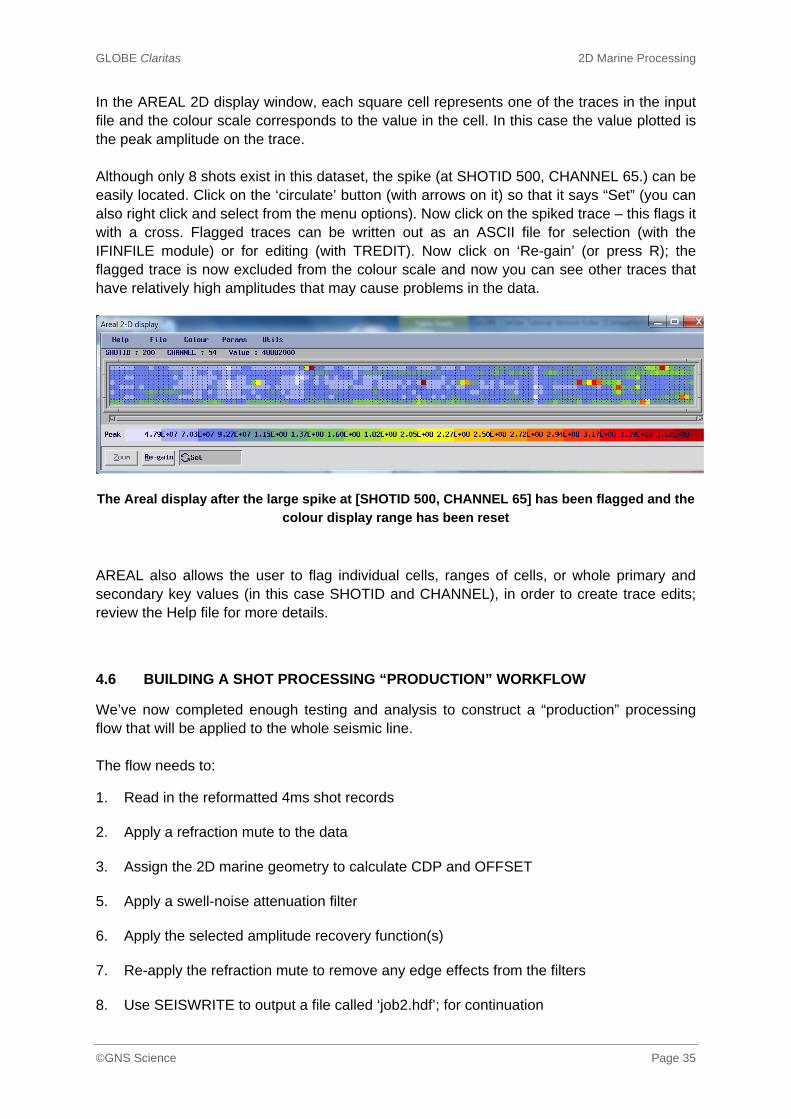
In the AREAL 2D display window, each square cell represents one of the traces in the input file and the colour scale corresponds to the value in the cell. In this case the value plotted is the peak amplitude on the trace. Although only 8 shots exist in this dataset, the spike (at SHOTID 500, CHANNEL 65.) can be easily located. Click on the ‘circulate’ button (with arrows on it) so that it says “Set” (you can also right click and select from the menu options). Now click on the spiked trace – this flags it with a cross. Flagged traces can be written out as an ASCII file for selection (with the IFINFILE module) or for editing (with TREDIT). Now click on ‘Re-gain’ (or press R); the flagged trace is now excluded from the colour scale and now you can see other traces that have relatively high amplitudes that may cause problems in the data.
The Areal display after the large spike at [SHOTID 500, CHANNEL 65] has been flagged and the
colour display range has been reset
AREAL also allows the user to flag individual cells, ranges of cells, or whole primary and secondary key values (in this case SHOTID and CHANNEL), in order to create trace edits; review the Help file for more details.
4.6 BUILDING A SHOT PROCESSING “PRODUCTION” WORKFLOW
We’ve now completed enough testing and analysis to construct a “production” processing flow that will be applied to the whole seismic line. The flow needs to:
1. Read in the reformatted 4ms shot records
2. Apply a refraction mute to the data
3. Assign the 2D marine geometry to calculate CDP and OFFSET
5. Apply a swell-noise attenuation filter
6. Apply the selected amplitude recovery function(s)
7. Re-apply the refraction mute to remove any edge effects from the filters
8. Use SEISWRITE to output a file called ‘job2.hdf’; for continuation
GLOBE Claritas 2D Marine Processing
©GNS Science Page 36
Expert User Tips:
‐ When you create output files or new SDE ASCII support tables, the ‘Edit’ and ‘List’ buttons
will point to the correct path and suggest the correct file extension to use automatically.
‐ You can use the F11 key to delete parameters in XSJE, or lines in XSDE and XEDT.
‐ ‘<Shift>+F11’ can be used to “paste” back the deleted line elsewhere.
‐ In SEISREAD, when you have entered the name of a disc file, if you press F12 (or the ‘Scan’
button) the parameter form will automatically be completed with the key details of your
file.
9. Use AREAL to output a PEAK value QC set for the whole line
10. Use AREAL to output an RMS value QC set for the whole line
11. Use an IF-ENDIF selection to write out a near trace dataset called ‘job2.ntp’
You can assemble the job yourself from the tests that have been run; use the ‘Include’ button in XSJE to add sections of existing workflows into the current flow. Simply highlight the range of modules that you want to include, and then modify any parameters.
The 4ms shot records are in a file called 434_job1.hdf5 in the ‘DATA’ directory.
You can investigate the contents and history of this file using the VIEW button in the SEISWRITE module, or by loading the file into the SV seismic viewer (‘Seismic Data’ tab on the Launcher).
Remember that you will need to change any REPEAT value to 1, and remove any trace selections if you copy a DISCREAD module from another job flow.
Alternatively, you can just review the GNS_job2.job processing flow.
4.7 QUALITY CONTROL PROCESSING FLOWS
Once the job has completed, you need to check that: There are no messages in the log file to indicate a problem
The output files exist and have the correct ranges of data in them
All of the traces were processed (based on the number of shots and channels)
Checking log files is often overlooked, but can tell you vital information.

GLOBE Claritas 2D Marine Processing
©GNS Science Page 37
Log file from the processing flow ‘GNS_job2.job’ showing information messages; errors
appear in red, and warnings in purple. The total trace count (10520 traces) corresponds to 876
shots (from 100 to 975) with 120 channels per shot

GLOBE Claritas 2D Marine Processing
©GNS Science Page 38
One key quality control step is to compare the input and output datasets to make sure that the processing flow has worked as anticipated. We typically do this by comparing a subset of the data and look for any variations.
The processing flow 06_job2_shotqc.job is designed to do this. If you open the flow and look at the SEISREAD module, you will notice that:
‐ instead of a seismic filename, a list file is given
‐ the parameter SETREPEAT has been set to ‘Yes’
If you use the ‘Edit’ button next to the LISTFILE parameter, you can see that the job is reading both the original HDF5 dataset, and the output from the ‘job2’ processing flow.
You may need to modify this to include your own output shots file from your production job, if you ran one.
Note how the primary key definition has been written after the file name, using the same format as the selection made in the 00_qc.job processing flow.
You can easily create this kind of comparison file using the XEDT text file editor (which opens when you press the ‘Edit’ button). Under the ‘File’ menu in XEDT, there is an option to ‘Include a list of DATA files’ – this will allow you to select from all the seismic files in the DATA directory, and populate the selection file (with the complete directory path).
The SETREPEAT parameter towards the end of the module has been set to ‘Yes’ so that each of the seismic files in the list will have a separate REPEAT value assigned to them. This ensures they will be plotted in different panels in XVIEW.
Run the job and compare the results. Note that in this case, the XVIEW display parameter has been set to be the same as the filename read in by SEISREAD. Review the data with and without an AGC applied and use the Analysis zoom windows to verify that the sequence has been applied correctly.
The second quality control dataset you created was a near-trace plot. The job 07_job2_ntpqc.job reads and displays the first 1000ms of this dataset.
Run this job, and then under the ‘Utils’ menu, select ‘Overlay offsets’. This option is designed to provide a useful QC of the geometry and shot timing. If you specify the velocity as 1500 ms-1 then a red line will be plotted where the theoretical first break should occur from the direct arrival.
Near trace QC display – allows checks such as the timing of the direct arrival (shown in red) so
that the near offset can be verified.

GLOBE Claritas 2D Marine Processing
©GNS Science Page 39
4.7.1 AREAL QC and Trace Editing
Go to the ‘Miscellaneous’ tab on the Launcher and start the Areal application; select the peak amplitude file (which is called GNS_job2_peak.are, if you are using the defaults).
Peak areal QC for the whole seismic line - peak trace amplitudes are colour coded; X-axis =
CHANNEL, Y-axis = SHOTID. ‘Warm’ colours are high amplitude values
If you looked at the test results with Areal, note that the parameter form will retain the values you entered before. Set the colour for flagged cells to be 32 (which corresponds to black) on the initial form or under ‘Params’. Immediately you should notice that:
CHANNEL 88 seems to be "quieter" that the others.
There are two spiked traces at the start of SHOTID 114 (CHANNEL 115 and 116).

GLOBE Claritas 2D Marine Processing
©GNS Science Page 40
Any long "noise trend" that dips from (in this case) from top right to bottom left indicates a strong signal that is moving down the cable as the boat moves; this probably corresponds to reflections or diffractions in the analysis window. Short noise trends, or those dipping in the opposite direction, are usually a result of swell-noise bursts or other bad data areas. If you click on the circulate button (with arrows on it), you activate the mouse button settings. Clicking again on the button cycles through the options. You can either "Set" marker flags, "Clear" them, or "Toggle" the flags on and off. There is also a “Test” option; hover the mouse across the colour-coded bar at the bottom and you can instantly test the effect of flagging cells above or below certain levels (specified by the mouse position). When you click on a given cell in "Set" or "Toggle" mode, it is flagged with a black X. A second click in "Toggle" or "Clear" mode removes the X. You can also hold down the left mouse button and drag the cursor over a range of values to flag, or use the P and S keys on the keyboard to flag a whole primary or secondary key. Set flags on the two noisy traces (SHOTID 115, CHANNEL 115, 116) then press the ‘Re-gain’ button (or press the R key on the keyboard); the display changes as the colour range is no longer dominated by the high amplitude traces you have flagged. There is sufficient redundancy in this dataset (it will be 60 fold) that if any give channel is being noisy we can afford to kill the whole trace rather than just edit out the noisy segment, as long as there are not too many adjacent channels being killed. When you have finished flagging cells select ‘File’ and ‘Write flags’. Call the file kill1.tre; this will be automatically saved into the ‘EDITS’ directory.
Expert User Tips:
‐ You can use the space‐bar as well as the mouse button to select data to flag (or unflag).
‐ Page‐up and Page‐Down can be used to step through the display.
‐ Open the output shot information (GNS_job2.hdf5) in SV (under the ‘Seismic Data’ tab)
and visually inspect the shots at the same time, verifying what you are flagging. Click on
the SHOTID label to jump to a shot number.

GLOBE Claritas 2D Marine Processing
©GNS Science Page 41
5.0 SORT TO CDP AND DECONVOLUTION
5.1 OBJECTIVES:
Creating a brute stack.
Plotting, hardcopy and side labels.
Using the WAVELET application to design filters.
XVIEW Autocorrelation Zoom Window.
ADDTIME parameters and their use with ZEROMUTE.
Gap Deconvolution design and application.
Adding autocorrelations to the bottom of a section.
QC of stacks in production jobs.
Text header and data value zoom.
Implications of CDP sorting.
5.2 CREATING A BRUTE STACK
With a dataset that has the geometry assigned, we can create a very basic or “brute” stack. We’ll use a very approximate set of velocities so that we have something to act as a comparison baseline for other tests. Open the 08_brute.job in the job flow editor. Things to notice in this job are: SEISREAD is reading the data in CDP/CDPTRACE order
The use of an automatic stretch mute in the NMO module.
There is no primary or secondary key in the STACK module; the data must be correctly sorted first!
Run the job. This will create a brute stack on the screen and save the stack file to disc. The STACK module automatically updates the HORI_SUM trace header to contain the fold (or number of live traces) stacked at any given CDP. This can be displayed on the seismic data to confirm that the stack has worked correctly.

GLOBE Claritas 2D Marine Processing
©GNS Science Page 42
Brute stack displayed with an AGC applied, and the fold plotted over the data (using the
‘Overlay CDP fold’ option under the ‘Utils’ menu)
5.2.1 Hardcopy of the Brute Stack
GLOBE Claritas™ produces plots in HP-RTL format – these can be directly plotted by any HP plotter without the need for additional software, and can be easily translated to a variety of formats with the utilities provided. The job 09_bruteplot.job is an example of a GLOBE Claritas™ plot job. The plotting part of the flow is in three parts; the seismic data (controlled by the RASTER module), the numbering of the traces and round-plot labelling (controlled by the PLOTLABEL module) and the side label (controlled by the SIDELABEL module), which contains processing and acquisition details. In this case, the processing history file is displayed in the side label, but you can specify any text you like in a separate "jdf" file.

GLOBE Claritas 2D Marine Processing
©GNS Science Page 43
A processing flow for generating a plot; the RASTER module has to come first, followed by
any labelling. A TOPLABEL module is also available for plotting statics, elevations etc.
The plot job creates an HPRTL file (in this case 09_brute.rtl) which can be submitted directly to any HP plotter or viewed using the Xrtl utility under the ‘Plotting’ tab on Launcher. To display the plot onscreen, specify a clockwise rotation and 40-50% scaling.
A plot visualised via the Xrtl utility prior to hardcopy, showing the top part of the side label and
display
A number of utilities exist to manipulate HPRTL files (convert to and from other formats, such as TIFF and Post Script) for use on other plotters and printers. See SeishelpUtilitiesRaster plots for full information.

GLOBE Claritas 2D Marine Processing
©GNS Science Page 44
5.3 MINIMUM PHASE CONVERSION AND THE WAVELET TOOL
The GLOBE Claritas™ filter design and wavelet manipulation tool is called Wavelet. It can be accessed from the ‘Wavelets’ tab on the Launcher. One of the key features of Wavelet is the ability to "Save" a session, so that an interactive workflow does not have to be repeated. Launch Wavelet and assign a name to the session in the first pop-up box. Click on the ‘(New)’ button, navigate to the “WAVELET” directory and select the signature file 434_sig.txt. Each Wavelet ‘memory cell’ is assigned a short name - call this one "Original" and click ‘OK’.
The Wavelet tool showing the initial source signature as a time series alongside its frequency
and phase spectra
We can apply various processes to the wavelet or to combinations of wavelets. First of all, click on the ‘?’ button in the Unary operations area - this allows you to select the input wavelet which will default to original. Next, hold down on the ‘Star’ button and select ‘Minphase’ from the list of operations; all operations will require some parameters, even if it is just the short name for the new cell. Type in “Minimum_Phase_Equivalent” and click ‘OK’.

GLOBE Claritas 2D Marine Processing
©GNS Science Page 45
The Wavelet tool showing the initial source signature and the minimum phase equivalent
Now click on the ‘?’ button in the Binary operations area and select the new wavelet; the original wavelet should still be selected on the first memory switch. Finally, hold down on the ‘Star’ button and select the ‘MatchFilt’ option. Type “Matching” as the name, with a length of 100 samples. You will see the following message; get into the habit of actually reading messages like these as they often contain valuable information.

GLOBE Claritas 2D Marine Processing
©GNS Science Page 46
The Wavelet tool showing the initial source signature, its minimum phase equivalent and the
matching filter to convert to minimum phase
This creates a matching filter which can be used to convert from the supplied source signature, to the minimum phase equivalent you created. You can test the application by filtering (convolving) the original wavelet with this matching filter; use the ‘Star’ button in the Binary section, convolving ‘Original’ with ‘Matching’. Finally we need to output the filter so that we can apply it to the data. Hold down the right mouse button on the cell containing the matching filter, and select ‘Output’. Type “434_MPCF” as the output filename (leave the format as a Text file), and click ‘OK’. The file 434_MPCF.wts will be created in the WAVELET directory. Full details of the functionality of the Wavelet application can be found in Seishelp.
GLOBE Claritas 2D Marine Processing
©GNS Science Page 47
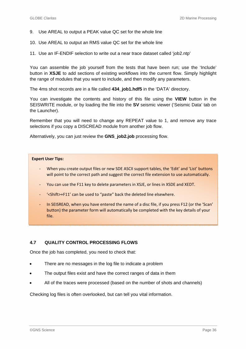
The processing flow 10_MPC.job shows the impact of applying the filter (using the
CONVCORR module) on the brute stack
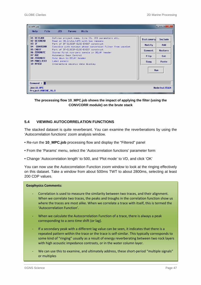
5.4 VIEWING AUTOCORRELATION FUNCTIONS
The stacked dataset is quite reverberant. You can examine the reverberations by using the ‘Autocorrelation functions’ zoom analysis window.
• Re-run the 10_MPC.job processing flow and display the "Filtered" panel
• From the ‘Params’ menu, select the ‘Autocorrelation functions’ parameter form
• Change ‘Autocorrelation length’ to 500, and ‘Plot mode’ to VD, and click ‘OK’
You can now use the Autocorrelation Function zoom window to look at the ringing effectively on this dataset. Take a window from about 500ms TWT to about 2800ms, selecting at least 200 CDP values.
Geophysics Comments:
‐ Correlation is used to measure the similarity between two traces, and their alignment.
When we correlate two traces, the peaks and troughs in the correlation function show us
where the traces are most alike. When we correlate a trace with itself, this is termed the
‘Autocorrelation Function’.
‐ When we calculate the Autocorrelation Function of a trace, there is always a peak
corresponding to a zero time shift (or lag).
‐ If a secondary peak with a different lag value can be seen, it indicates that there is a
repeated pattern within the trace or the trace is self‐similar. This typically corresponds to
some kind of “ringing” usually as a result of energy reverberating between two rock layers
with high acoustic impedance contrasts, or in the water column layer.
‐ We can use this to examine, and ultimately address, these short‐period “multiple signals”
or multiples
GLOBE Claritas 2D Marine Processing
©GNS Science Page 48
The filtered brute stack with an ‘Autocorrelation functions’ zoom window displayed, showing
the pattern of reverberations in the data
5.5 TESTING WEINER DECONVOLUTION BEFORE STACK
We can use repeat panel tests to look at the effect of different deconvolution parameters on the reverberations we observed. The processing flow 11_DBS_shots.job displays a selection of shots with six different suites of deconvolution parameters.
Geophysics Comments:
‐ Weiner deconvolution (aka: gap or predictive deconvolution) is a statistical method for
shaping the source wavelet. While it can be used to “whiten” the signal (and enhance the
higher frequencies), in marine processing its main use is to collapse a reverberant wavelet.
‐ The design of the deconvolution filter is based on an autocorrelation function; it is
important to specify this “design window” such that it contains data, as opposed to noise,
and avoids any high amplitude events (such as the seafloor).
‐ It is possible to have multiple design gates – for example above and below a strong, high
amplitude event – and correspondingly, multiple application gates.
‐ Other key parameters are the “gap” or lag of the predictive filter, and the length of the
calculated operator. The gap will impact the frequency content, with smaller gaps creating
a compressed wavelet. In general, the operator should be long enough to include the
reverberations however the design window needs to be at least 4‐5 times the operator
length, for stability.

GLOBE Claritas 2D Marine Processing
©GNS Science Page 49
Weiner deconvolution is applied in GLOBE Claritas™ using the DECONW module.
As with other GLOBE Claritas™ modules, the parameters that can vary spatially; the application and design windows, as well as the gap and operator length of the filter, are all stored in a separate parameter file that can be edited using the XSDE control files editor.
Typically the user would design windows based on SHOTID and CHANNEL (or OFFSET), however in this case we are going to use the ADDTIME feature in many GLOBE Claritas™ modules.
We’ll use the ZEROMUTE module to store the time of the first live sample in the DELAY header, and then define a single window that will start below this time – essentially we are using the refraction mute to vary the deconvolution design window.
The processing flow 11_DBS_shots.job which shows the effect of applying
deconvolution to the shots
Expert User Tips:
‐ The SMUTE module has a NO APPLY option, as well as the possibility to store a mute in a
trace header. This allows you to create a start‐time for the design gate based on any
picked mute file, not just one that has been applied.
‐ The time of the first live sample is stored in the DELAY header using the ZEROMUTE
module; this allows the design and application gates of the deconvolution to be relative to
the start of the data, simplifying the parameterisation of the windows.
‐ You can also digitise a horizon and use the ADDDIG module to store this horizon time
(from a stack or near trace plot) as the basis for a deconvolution design.
‐ These techniques can be combined to create processing sequences that vary with water
depth.

GLOBE Claritas 2D Marine Processing
©GNS Science Page 50
The control file for the deconvolution has been set up to vary with REPEAT. This, coupled with the use of ADDTIME, allows us to create a series of test panels to easily review different parameters for deconvolution.
The parameter control file used in 11_DBS_shots.job to vary the operator length in the
deconvolution with the value of the REPEAT primary key
Run the job, and review the results. To help you, the autocorrelation function is now automatically appended to the bottom of the display; created using the same definitions (based on ADDTIME) as the design window for the deconvolution.
You can use the number keys on the keyboard (or the mouse) to animate between the panels – the differences can be quite subtle and this animation can help you to see small changes.
Note how the panels are labelled automatically, so that if you change the deconvolution parameters, the display is updated.

GLOBE Claritas 2D Marine Processing
©GNS Science Page 51
We should also look at the impact of the deconvolution on the stacked section; to do this we have to apply different deconvolution and then stack the data. The processing flow 12_DBS_stack.job does this, using only a small subset of the data to speed up the processing flow.
The processing flow 12_DBS_stack.job, designed to compare stacked panels with
deconvolution-before-stack (DBS) applied
Both of these flows can be modified to look at the effects of changing the gap. We would typically test gaps of 4ms, 8ms, 16ms, 24ms, 32ms and 48ms on this type of data.
You can modify the existing lines in the control file to do this, or add new lines and extend the number of repeats in the SEISREAD module.
Expert User Tips:
‐ In addition to a conventional gap in milliseconds, you can also specify the gap in terms of
the Nth zero crossing of the autocorrelation function. To do this, specify a negative integer
in the gap, so that (for example) ‐2 is the second zero crossing and so on.
‐ You can apply a spiking deconvolution by specifying a gap of zero.
‐ The module SCDECON can be used to create shot‐consistent deconvolution where the
autocorrelation function is averaged across all of the input traces in a shot (or receiver)
gather.

GLOBE Claritas 2D Marine Processing
©GNS Science Page 52
5.5.1 Applying Deconvolution and Sorting the Data
We’ve now completed enough testing and analysis to construct a “production” processing flow that will be applied to the whole seismic line.
The flow needs to:
Read in the data from Job 2.
Apply any trace edits from the AREAL QC displays.
Apply the minimum phase conversion filter.
Apply our selected gap deconvolution.
Output a file containing CDP-ordered post-DBS data: job3.hdf5
An example of the job flow for Job 3; this is an example that you could modify to include your
own files and parameters
Try setting this job up, and compare it to GNS_job3.job. You will have to set up a new deconvolution control file to apply your selected parameters using XSDE.
Expert User Tips:
‐ You could also include a stack on the end of this processing flow to create an additional
QC; while we will do this in the next stage, the critical module to include in this case would
be GENSORT in order to be able to sort the data into CDP order before stacking. While
there is a module called CDPSORT, this is for use with full land geometry and not a simple
marine geometry.

GLOBE Claritas 2D Marine Processing
©GNS Science Page 53
5.5.2 Checking the Results
Once the job has completed, you need to check that: There are no messages in the log file to indicate a problem
That the output files have been created and have the right number of traces in them The processing flow 13_stack.job creates the QC stack; it is much the same as the brute stack we looked at earlier just with a different input and output file. An extremely useful QC step is to create ‘compare’ jobs for both shots and stacks. Each time a new file is created, you can add it to this compare job to easily see your progress while processing. The jobs 14_stack_compare.job and 15_shot_compare.job can be used to look at the results of the processing sequence so far.
The DBS stack displayed with the fold overlaid – note how the fold varies as a result of the
edits we have made
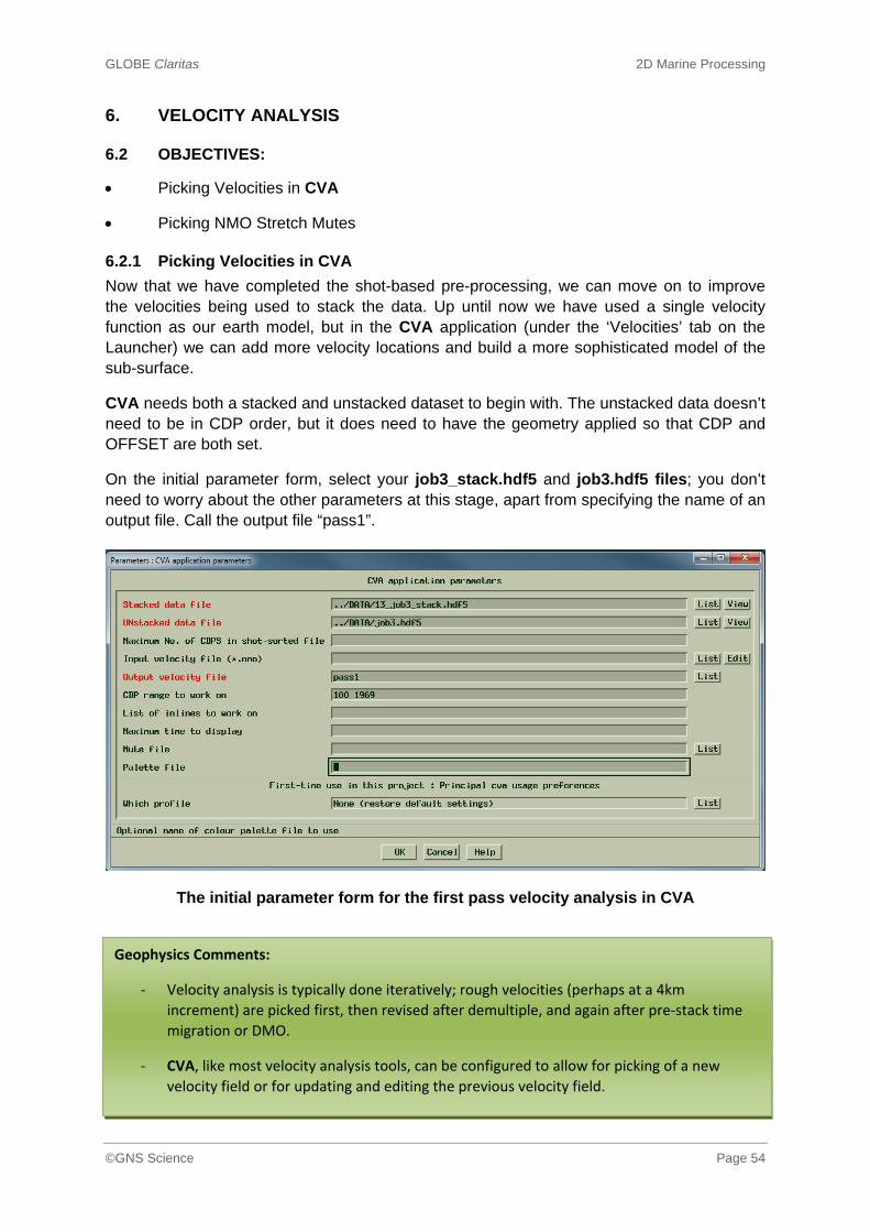
GLOBE Claritas 2D Marine Processing
©GNS Science Page 54
6. VELOCITY ANALYSIS
6.2 OBJECTIVES:
Picking Velocities in CVA
Picking NMO Stretch Mutes
6.2.1 Picking Velocities in CVA
Now that we have completed the shot-based pre-processing, we can move on to improve the velocities being used to stack the data. Up until now we have used a single velocity function as our earth model, but in the CVA application (under the ‘Velocities’ tab on the Launcher) we can add more velocity locations and build a more sophisticated model of the sub-surface.
CVA needs both a stacked and unstacked dataset to begin with. The unstacked data doesn’t need to be in CDP order, but it does need to have the geometry applied so that CDP and OFFSET are both set.
On the initial parameter form, select your job3_stack.hdf5 and job3.hdf5 files; you don’t need to worry about the other parameters at this stage, apart from specifying the name of an output file. Call the output file “pass1”.
The initial parameter form for the first pass velocity analysis in CVA
Geophysics Comments:
‐ Velocity analysis is typically done iteratively; rough velocities (perhaps at a 4km
increment) are picked first, then revised after demultiple, and again after pre‐stack time
migration or DMO.
‐ CVA, like most velocity analysis tools, can be configured to allow for picking of a new
velocity field or for updating and editing the previous velocity field.
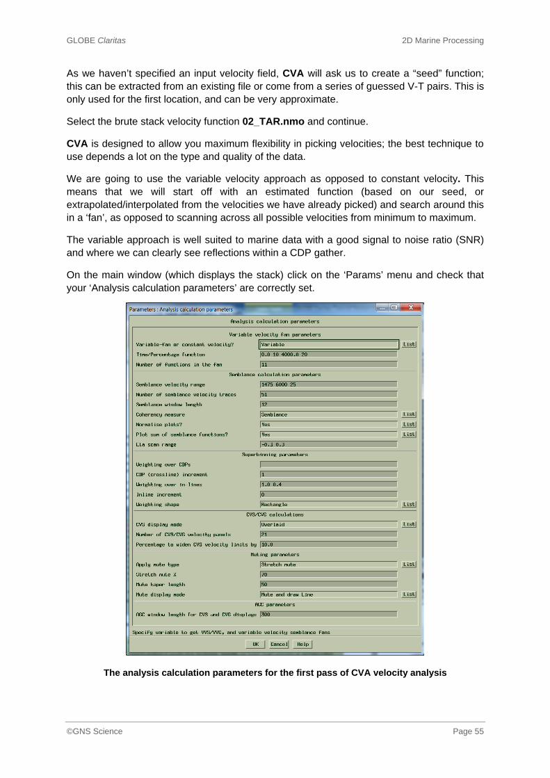
GLOBE Claritas 2D Marine Processing
©GNS Science Page 55
As we haven’t specified an input velocity field, CVA will ask us to create a “seed” function; this can be extracted from an existing file or come from a series of guessed V-T pairs. This is only used for the first location, and can be very approximate.
Select the brute stack velocity function 02_TAR.nmo and continue.
CVA is designed to allow you maximum flexibility in picking velocities; the best technique to use depends a lot on the type and quality of the data.
We are going to use the variable velocity approach as opposed to constant velocity. This means that we will start off with an estimated function (based on our seed, or extrapolated/interpolated from the velocities we have already picked) and search around this in a ‘fan’, as opposed to scanning across all possible velocities from minimum to maximum.
The variable approach is well suited to marine data with a good signal to noise ratio (SNR) and where we can clearly see reflections within a CDP gather.
On the main window (which displays the stack) click on the ‘Params’ menu and check that your ‘Analysis calculation parameters’ are correctly set.
The analysis calculation parameters for the first pass of CVA velocity analysis

GLOBE Claritas 2D Marine Processing
©GNS Science Page 56
For picking velocities, we want to use a regular spatial increment; picking functions from the start-time to the end time. For now, we also want to be able to jump straight to a location that has already been picked from the stack (or the isovels display window), to modify it.
The ‘Analysis location parameters’ form should look like this:
The analysis location parameters for the first pass of CVA velocity analysis
There are three options for the ‘Analysis positioning’: (i) At nearest existing V(t) (ii) At pointer, and (iii) Click and drag. In the first two of these, you select an analysis window by clicking on the main stack window (or isovels window); the analysis is then located at the nearest velocity function, or where you position the pointer. In ‘Click and drag’ mode, you can choose a time and space window using the mouse and “layer strip” across and down the section. These different modes give you the flexibility to follow complex geological events and refine velocities in those areas.
The final parameter form allows further options, and should look like this:
The parameter form that controls user defined behaviours for the windows

GLOBE Claritas 2D Marine Processing
©GNS Science Page 57
Now that you know where the main controls are, and we have checked that they are correctly set, you can move on to picking velocities.
You can adjust the main stack display in the same way as you modified XVIEW; this includes applying an AGC or balance, modifying the colour maps and adjusting how they match to the amplitude ranges.
The current area for velocity analysis is marked by a blue box. As you pick velocities, these will also be labelled.
Click on the ‘Semblance’ button and then on the ‘Gathers’ button in the semblance window.
Variable Velocity semblance spectra and gather, prior to picking. The semblance spectra are
calculated in a ‘fan’ around the initial velocity estimate
As with picking mutes, use the left mouse button to add, delete or move a pick. As you pick, the gather will be NMO corrected. At any stage you can use the ‘Recompute’ button (or press the C key) to recalculate the velocity ‘fan’ centred on the current picks.
The ‘Vels’ button in the ‘Gathers’ window can be used to display the velocities and NMO curves.
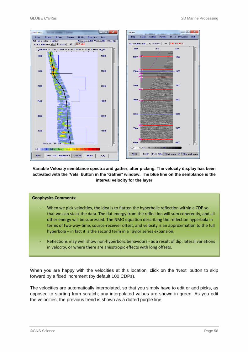
GLOBE Claritas 2D Marine Processing
©GNS Science Page 58
Variable Velocity semblance spectra and gather, after picking. The velocity display has been
activated with the ‘Vels’ button in the ‘Gather’ window. The blue line on the semblance is the
interval velocity for the layer
When you are happy with the velocities at this location, click on the ‘Next’ button to skip forward by a fixed increment (by default 100 CDPs). The velocities are automatically interpolated, so that you simply have to edit or add picks, as opposed to starting from scratch; any interpolated values are shown in green. As you edit the velocities, the previous trend is shown as a dotted purple line.
Geophysics Comments:
‐ When we pick velocities, the idea is to flatten the hyperbolic reflection within a CDP so
that we can stack the data. The flat energy from the reflection will sum coherently, and all
other energy will be supressed. The NMO equation describing the reflection hyperbola in
terms of two‐way‐time, source‐receiver offset, and velocity is an approximation to the full
hyperbola – in fact it is the second term in a Taylor series expansion.
‐ Reflections may well show non‐hyperbolic behaviours ‐ as a result of dip, lateral variations
in velocity, or where there are anisotropic effects with long offsets.

GLOBE Claritas 2D Marine Processing
©GNS Science Page 59
The isovels display can be used to view and edit your velocity field. This view - coupled with the ability to view the previous and next velocity functions - helps you to get to a more accurate velocity model faster.
The isovels display; this is linked to your picking and updates as you make picks.
Expert User Tips:
‐ The automatic interpolations options are designed to let you effectively and rapidly pick
datasets. If you set the analysis positioning to be “At pointer”, you can then set a velocity
function at the start and the end of the line – simply click on the stack or the isovels plot
where you want to pick.
‐ Set the picking increment to be coarse – double or four times the resolution you need –
on the ‘Analysis location’ parameter form and then step quickly through the dataset.
After this first pass, change the increment and step back through, infilling velocities.
‐ The interpolation allows you to make fewer and fewer picks, as you are simply modifying
the automatically interpolated picks.
‐ Where you have channels or rapid variations of structure, you can simply add a new
location outside of the fixed increment pattern.

GLOBE Claritas 2D Marine Processing
©GNS Science Page 60
You can use the isovels display to navigate to locations for analysis; simply double-click to move to a given location. You can also use it to edit or manipulate velocities. The options to add and remove velocity functions (or values) can be accessed using the ‘circulate’ button, marked with circular arrows and labelled “(keyboard)”. The isovels display in CVA is a version with limited functionality, much in the same way that the stack is displayed in an XVIEW window with limited capabilities. The full version of isovels includes smoothing, editing and velocity conversion functionality and can be accessed from the ‘Velocities’ tab on the Launcher.
Constant velocity stacks (CVS), in addition to semblance-based picking on variable velocities, can be useful on noisy data or over a limited time range (especially in the shallow part of the section). The best way to configure these is to use a fixed spatial increment, and set a limited time window range of (say) 1000ms. It is useful to display enough CDPs such that you can see three velocity functions at a time. Close down the ‘Semblance’ and ‘Gather’ displays. Select ‘Params’ and go to the ‘Analysis calculation parameters’ form; switch from “Variable” to “Constant” in the first field. You also need to make sure that the ‘CVS display mode’ field is set to “Overlaid”. The ‘Analysis calculation parameters’ form should look like this:
Geophysics Comments:
‐ In general, you need to make velocity picks at least 100ms TWT apart; closer than this can
create instability in the velocity function and interval velocity analysis display.
‐ While picking, it’s worth keeping an eye on the interval velocity displays to see if they are
realistic. For example, 1500m/s is the speed of sound in water; an interval velocity close
to this value on marine data may indicate that you are picking multiples
‐ Sandstones and mudstones on the seafloor that have not been compacted and inverted
tend have low interval velocities, rising slowly from 1600m/s or so. Limestone tends to
have a velocity of around 3000‐3700m/s. Halite (salt) has a velocity of 4500m/s.
‐ Interval velocities are unlikely to be higher than 5500‐6000 m/s, even in the hardest
metamorphic and igneous rocks. Velocities higher than this are likely to be diffractions or
out‐of plane.
‐ The stacking velocity generally increases with depth; inversions are possible but unusual.

GLOBE Claritas 2D Marine Processing
©GNS Science Page 61
Configuring CVA for constant velocity stack analysis on the ‘Analysis calculation parameters’
form
Next, configure the ‘Analysis location parameters’ form to have a fixed time range as follows:
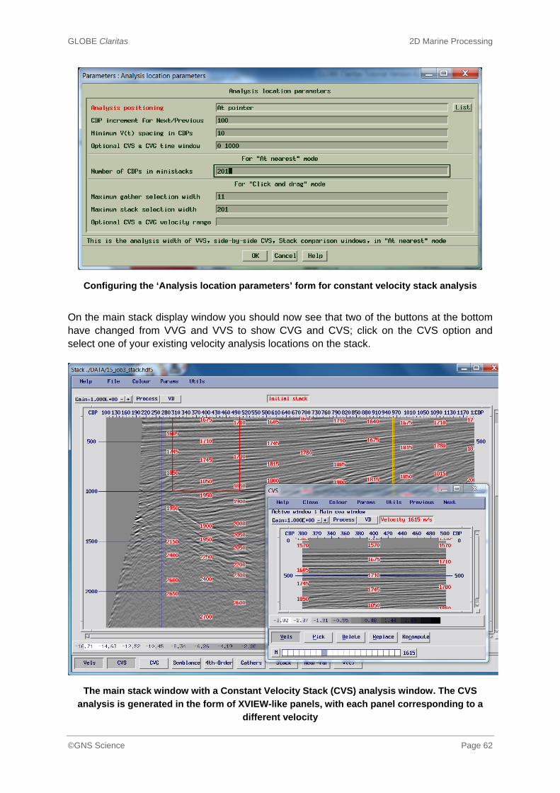
GLOBE Claritas 2D Marine Processing
©GNS Science Page 62
Configuring the ‘Analysis location parameters’ form for constant velocity stack analysis
On the main stack display window you should now see that two of the buttons at the bottom have changed from VVG and VVS to show CVG and CVS; click on the CVS option and select one of your existing velocity analysis locations on the stack.
The main stack window with a Constant Velocity Stack (CVS) analysis window. The CVS
analysis is generated in the form of XVIEW-like panels, with each panel corresponding to a
different velocity

GLOBE Claritas 2D Marine Processing
©GNS Science Page 63
You can “lock” the velocity range of the CVS display in the ‘Analysis location parameters’ form, or change the defaults in the pop-up window that appears. A red rectangle marks the selected data for the CVS displays, which are presented as separate panels similar to those in XVIEW.
Click on the ‘Vels’ button to display the velocities on the panels; animate between them using the mouse or arrow keys. Picking in CVS mode uses the ‘Pick’, ‘Delete’ and ‘Replace’ buttons – although in practice it is much easier to use the mouse with one hand, and activate the picking mode with the other using the keyboard (P, D and R keys). You can change the range of velocities at any time using the ‘Recompute’ button.
When using CVS displays, it is best to step through the data with the ‘Previous’ and ‘Next’ buttons, and then modify the time range in the parameter form to the next “layer” down, with some degree of overlap.
Geophysics Comments:
When working with constant velocity stacks (CVS) or gathers (CVG):
‐ If the reflections are not flattened on ANY of the panels (CVG) or the stack is only
improving in the last few panels, you can redefine the velocity range using the
‘Recompute’ button.
‐ Use small time windows (1000‐1500ms maximum) to ensure you limit the velocity range
and hence maintain velocity resolution.
‐ You should aim to “layer strip” the dataset, in overlapping layers, using the ‘Previous’ and
‘Next’ buttons.
‐ You can add new functions if needed – for example from the isovels display.
‐ You can use the ‘Stack’ button on the main display to compare the results with your new
velocity function.
Expert User Tips:
‐ You can have CVS and CVG displays active and linked, with semblance spectra, NMO‐
corrected gather and on‐the‐fly mini‐stack all displayed at the same time.
‐ You can use variable velocity stacks (VVS) and gathers (VVG) based on a “fan” of functions
around the current velocity estimate.
‐ You can display the CVS, CVG or VVS, VVG panels side‐by side, and pick a function across
the different panels.
‐ You can choose where to do an analysis on the stack display, and control the spatial
and/or time extent of the window, by using the “Click and drag” option.

GLOBE Claritas 2D Marine Processing
©GNS Science Page 64
6.3 PICKING NMO STRETCH MUTES
Up until now we have been using an automatic stretch mute. This works reasonably well at depth, but in the shallow part of the section the NMO stretch can be significant. In particular, it can result in the sea-floor reflection being muted.
You can pick an NMO stretch mute at any time on the ‘Gather’ window by clicking on the ‘Pick Mute’ button, although it is often best to do this when picking velocities in Semblance-mode. Picking is done using the left mouse button (as with SV); a blue line shows the picked mute, and a purple line shows the automatic (percentage) stretch mute. The user can toggle which mute is displayed (and used). In the ‘Gather’ window, the picked mute is displayed as a blue line, and the automatic stretch mute as a purple one. The blue line is thin when the mute is interpolated, and thick (with control points) at the location(s) where it has been picked and can be edited. You can control which mute is applied (across all the analysis windows) using the mute ‘circulate button’ or in the parameter form. Existing mutes can be loaded on the initial parameter form or from the ‘File’ menu. Mutes can be saved at any time from the ‘File’ menu. Mute locations are shown on the stacked section display with a small blue arrow marker. Once you have picked a stretch mute, call it “pass1”. When you have finished picking and want to exit you will be prompted to save the velocity field (and mute if you created one); if you attempt to overwrite the input field, or a file you have already saved, you will be prompted with a warning.
Geophysics Comments:
‐ NMO stretch occurs when the NMO correction is very large ‐ usually in the shallow part of
the section, at far offsets, and with low velocities. In these situations, the reflection
hyperbola on a CDP gather is very large and can extend across a significant two‐way‐time
range. This can mean that for a particular event, the NMO correction that is applied at the
top of the waveform is larger than the correction at the bottom; as a result when the
NMO correction is applied, the event becomes “stretched” forming a ‘trumpet’ shape at
the far offsets.
‐ This stretched data needs to be excluded from the stack as it will introduce low frequency
artefacts.
‐ We can do this automatically – based on a percentage of how much stretch can take place
before muting – or we can manually pick a mute to remove it, in the same way we did for
refractions.

GLOBE Claritas 2D Marine Processing
©GNS Science Page 65
Picking a mute in the ‘Gather’ window alongside a semblance velocity analysis
CVA also retains a “profile” that contains all of the display and configuration parameters you have used; you can save a profile (and name it). When you restart CVA you can select a named profile, revert to the last profile used, or start afresh.
6.4 CHECKING VELOCITIES AND MUTES WITH SV
You can QC the velocities and mutes you have developed using SV (under the ‘Seismic Data’ tab on the Launcher).
On the main SV form, select job3.hdf5 (the pre-processed shots) as the input seismic file. By default this will appear displayed in SHOTID/CHANNEL order.
Next, click on the ‘File’ menu, select ‘Load input file’ and find the mute file you picked (mutes are located in the ../COMMON/MUTES directory).
The mute will be displayed, even though it was picked on CDP ordered data.
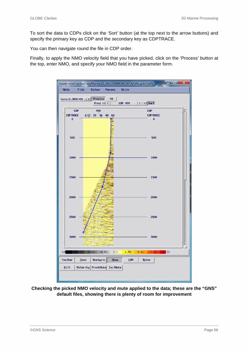
GLOBE Claritas 2D Marine Processing
©GNS Science Page 66
To sort the data to CDPs click on the ‘Sort’ button (at the top next to the arrow buttons) and specify the primary key as CDP and the secondary key as CDPTRACE.
You can then navigate round the file in CDP order.
Finally, to apply the NMO velocity field that you have picked, click on the ‘Process’ button at the top, enter NMO, and specify your NMO field in the parameter form.
Checking the picked NMO velocity and mute applied to the data; these are the “GNS” default files, showing there is plenty of room for improvement
GLOBE Claritas 2D Marine Processing
©GNS Science Page 67
6.4.1 Creating a QC stack
We now need to stack this dataset so that we can see the improvement on the stacked sections as well. The processing flow 16_newstack.job is set up to do this with the GNS defaults, so you will need to use your own input seismic file, mute, and velocity field.
To compare the results, you could use the processing flow 14_stack_compare.job and add the new stack file into the list file 14_stack.sfl. If you open the flow and the SEISREAD module, click on the ‘Edit’ button to open the list file where you can either:
Manually add the path name
Click on the ‘File’ menu, select ‘Include a list of DATA files’ and then select the file(s) you want to add to your selection
The job 17_stack_compare.job has been set up for you if you prefer.
This kind of “rolling QC” where you check both stacked and unstacked data at every stage of processing to ensure that you have the improved the results, is a key stage in seismic processing. The use of panels and list-selection files in GLOBE Claritas™ makes this particularly easy.
If you are unhappy with your velocities or mutes, you may need to go back and change them.
7. IMPROVING VELOCITY ANALYSIS: ANTI-MULTIPLE AND PRESTM
7.1 OBJECTIVES:
RADON demultiple and parameterisation
Using super gathers in marine processing
FK filters and spatial aliasing
Quality control after demultiple
Pre-stack time migration
7.2. RADON DEMULTIPLE THEORY
This dataset has some significant multiples, which make accurate velocity analysis difficult. We could probably suppress most of these just by stacking with the correct velocity, but it is hard to see the primary energy in order to pick it.
The RADON demultiple in GLOBE Claritas™ (PRT_DEMULT) splits the input data into a series of parabolic curves. With an NMO correction applied, and for reasonable angles, an originally hyperbolic seismic reflection matches to a parabola quite well. The data can then be muted or modelled based on the curvature of these parabolas.
The curvature is expressed in terms of the "far offset moveout" i.e. how many milliseconds above or below the current "zero offset" NMO corrected time the parabola would be on the

GLOBE Claritas 2D Marine Processing
©GNS Science Page 68
far offset trace. By modelling and removing the moveout values that correspond to the multiples, we can subtract these from the data leaving only the primary and any un-modelled noise.
In this example, we will correct the primary data to be flat (i.e. have close to zero moveout at the far offset) and then reject the down-dipping parabolic energy of the multiples. If your primaries are down dipping, or you have picked a multiple velocity trend, it won’t be very effective!
The RADON transform is implemented through the application of a matrix which depends, amongst other parameters, on the distribution of offsets within a CDP. Since we have "odd" and "even" CDPs with different offset distributions, we would need two separate matrices to transform them. These matrices can be very large (100Mb or more) and require considerable computational time at the start of the job. An alternative approach is to use a single matrix, and interleave an odd and even CDP to make a single "supergather" that contains all of the offsets.
We can also save the transform matrix, so that re-runs of the job that use the same transform parameters (but perhaps different multiple model parameters) run much faster.
This "supergather" process also helps to improve the resolution in the transform domain, and reduce artefacts that might arise as a result of spatial aliasing.
7.2.1 Testing and Applying RADON Demultiple
The processing flow 18_radon_cdp.job has been configured to demonstrate how to test the RADON demultiple; it uses the GNS default file names, so the input seismic and velocity field may need to be updated.
The RADON demultiple testing flow, 18_radon_cdp.job
GLOBE Claritas 2D Marine Processing
©GNS Science Page 69
When the job has been run once, the matrix for the radon transform is saved. After you have run the job for the first time, you can at this point flip module 09 “off” (which saves the matrix after calculation) and flip module 10 on (which reads in a saved matrix). This job reads in two CDPs from the middle of the line, duplicates them, and runs one copy through the RADON demultiple sequence outlined above. In addition to the RADON demultiple, you will notice that FK-filters are also used. FK domain filters (aka: dip filters) can also be used to suppress multiples simply by removing any down dipping (as opposed to down-curving) energy after an NMO correction is applied. Read the description of this module (using the ‘Dictionary’ button) for more details. In this case, the main function of the FK-filters is to remove any steeply dipping linear noise that may be aliased in the RADON domain, and to remove any artefacts that the transform may introduce. Run the processing flow, and look at the impact of the RADON demultiple on the CDP’s. This job will run quite slowly, despite the fact it has only two CDP’s to read. This is because it creates (and writes out) a large matrix that is used as part of the RADON transform. After it has run for the first time, you can flip the module 09 “off” and activate module 10 instead, which is configured to read back the saved matrix. The job uses REPEAT and a series of IF/ENDIF loops so that you can see the impact of each of the filters. Use the ‘FK spectrum’ analysis window to see what impact the FK filters have on the data.
Expert User Tips:
‐ You can measure the far‐offset moveout with the parabolic ruler. To activate this, click on
the ‘Ruler’ button with the right mouse button.
‐ You will be prompted for the reference offset, enter “3208” (the far offset, in metres).
‐ Click once with the left mouse button to start drawing the parabola, a second click to exit.
‐ The ruler and most recent measurements are retained on the display and can be used to
help parameterise the RADON demultiple.
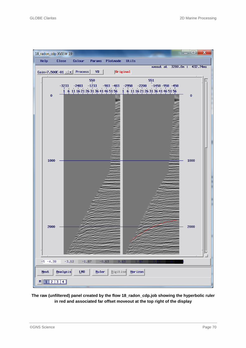
GLOBE Claritas 2D Marine Processing
©GNS Science Page 70
The raw (unfiltered) panel created by the flow 18_radon_cdp.job showing the hyperbolic ruler
in red and associated far offset moveout at the top right of the display

GLOBE Claritas 2D Marine Processing
©GNS Science Page 71
Another useful QC of the demultiple processing is to create difference plots; on the ‘Utils’ menu select ‘Plot Difference’ and in the pop-up window for the panels enter “1” and “4”, separated by a space. If you toggle between these panels on the display before selecting plot difference, this will be the default. A new panel (5) will be created displaying the difference between these two displays.
The difference plot between the raw data (panel 1) and the final data (panel 4); note how some
primary energy is also being removed
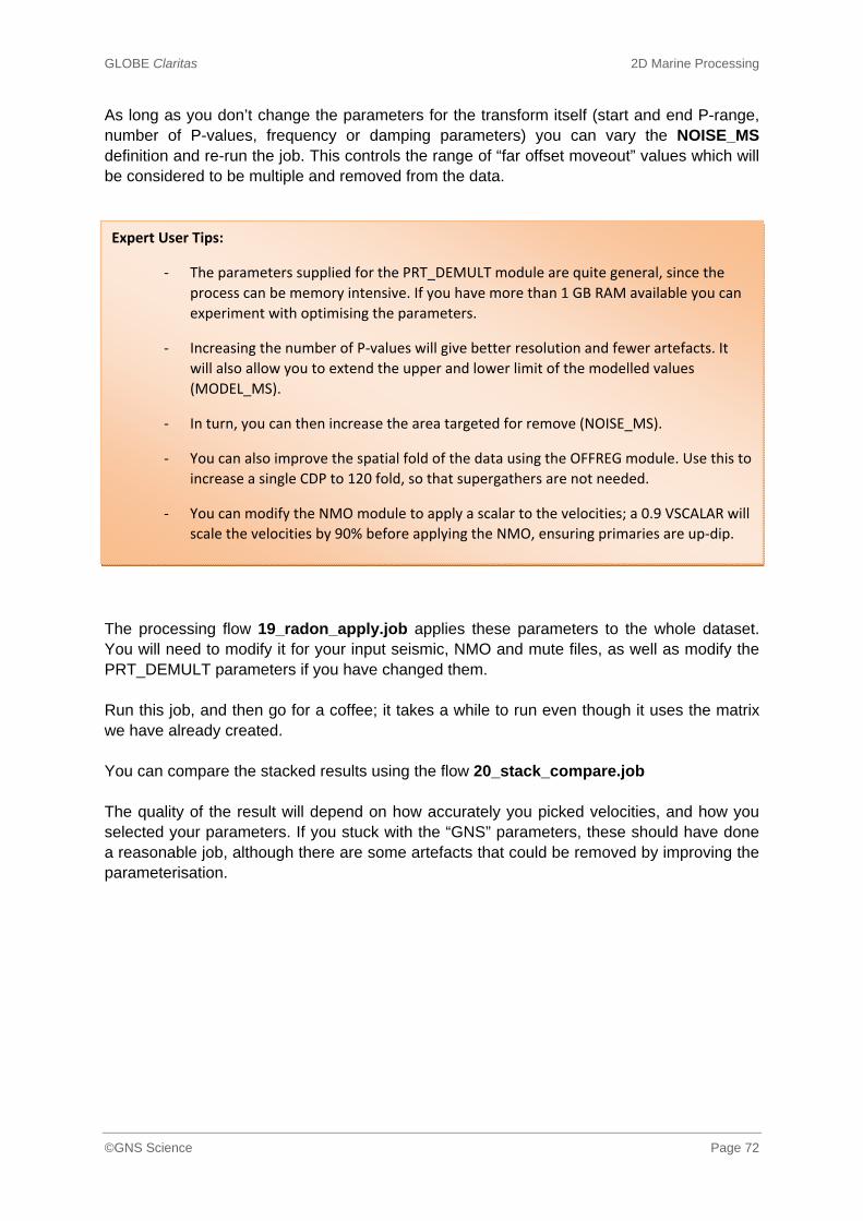
GLOBE Claritas 2D Marine Processing
©GNS Science Page 72
As long as you don’t change the parameters for the transform itself (start and end P-range, number of P-values, frequency or damping parameters) you can vary the NOISE_MS definition and re-run the job. This controls the range of “far offset moveout” values which will be considered to be multiple and removed from the data.
The processing flow 19_radon_apply.job applies these parameters to the whole dataset. You will need to modify it for your input seismic, NMO and mute files, as well as modify the PRT_DEMULT parameters if you have changed them. Run this job, and then go for a coffee; it takes a while to run even though it uses the matrix we have already created. You can compare the stacked results using the flow 20_stack_compare.job The quality of the result will depend on how accurately you picked velocities, and how you selected your parameters. If you stuck with the “GNS” parameters, these should have done a reasonable job, although there are some artefacts that could be removed by improving the parameterisation.
Expert User Tips:
‐ The parameters supplied for the PRT_DEMULT module are quite general, since the
process can be memory intensive. If you have more than 1 GB RAM available you can
experiment with optimising the parameters.
‐ Increasing the number of P‐values will give better resolution and fewer artefacts. It
will also allow you to extend the upper and lower limit of the modelled values
(MODEL_MS).
‐ In turn, you can then increase the area targeted for remove (NOISE_MS).
‐ You can also improve the spatial fold of the data using the OFFREG module. Use this to
increase a single CDP to 120 fold, so that supergathers are not needed.
‐ You can modify the NMO module to apply a scalar to the velocities; a 0.9 VSCALAR will
scale the velocities by 90% before applying the NMO, ensuring primaries are up‐dip.
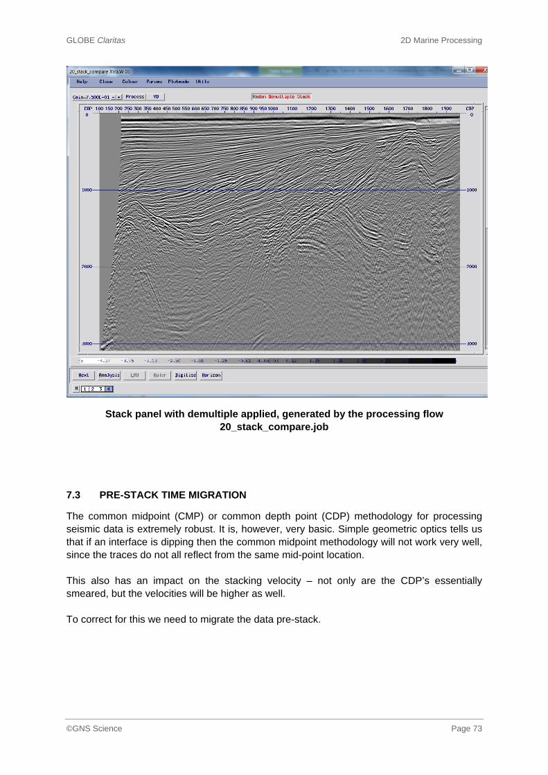
GLOBE Claritas 2D Marine Processing
©GNS Science Page 73
Stack panel with demultiple applied, generated by the processing flow 20_stack_compare.job
7.3 PRE-STACK TIME MIGRATION
The common midpoint (CMP) or common depth point (CDP) methodology for processing seismic data is extremely robust. It is, however, very basic. Simple geometric optics tells us that if an interface is dipping then the common midpoint methodology will not work very well, since the traces do not all reflect from the same mid-point location. This also has an impact on the stacking velocity – not only are the CDP’s essentially smeared, but the velocities will be higher as well. To correct for this we need to migrate the data pre-stack.

GLOBE Claritas 2D Marine Processing
©GNS Science Page 74
KPRET2D is the GLOBE Claritas™ 2D Kirchhoff PreSTM module; it is effectively a stand-alone module in that it cannot be used with any other modules in a processing flow.
We need to prepare the data for the Kirchhoff PreSTM by applying a couple of corrections. The first is to remove the spherical divergence correction, since the migration is kinematic and will correct for spherical spreading. The second correction is to overcome an approximation used in KPRET2D. Kirchhoff migration utilises the time derivative of the trace, and not the actual trace amplitudes. In KPRET2D, this is currently (V6.0) approximated by a phase rotation.
We can obtain a better result (with a higher frequency content) if we differentiate the trace and counter the phase rotation within the preparation stage.
NB: If you are using a more recent release than V6.0 please check the dictionary for the KPRET2D module and ensure that the derivative and phase shift modules are still required.
Geophysics Comments:
‐ Migration uses a mathematical model of the sub‐surface to correct for how the wavefield
is scattered by interfaces that are not flat. Migration routines require some kind of
velocity field – as a rule of thumb the more sophisticated the migration, the more complex
the velocity field and the longer the run time.
‐ Post‐stack migration used to be the ‘workhorse” of the industry however it could not
account for the impact of dip and structure on stacking velocities. Dip Moveout (DMO)
was introduced as a partial pre‐stack time migration, to correct for dipping events. Full
pre‐stack time migration (PreSTM) has become increasingly routine over the last decade.
‐ Our initial estimate of velocities is likely to be contaminated with dip, diffraction energy
and (in our case) multiples. It is routine to re‐pick velocities (or residual moveout) after
PreSTM, create a new velocity field, and then re‐run the pre‐stack time migration.
‐ The output from the PreSTM are gathers corrected to zero offset, which account for both
the normal‐moveout correction and any dip. We need to remove the effect of the NMO
correction in order to update the velocity field.
Expert User Tips:
‐ When an input trace is being migrated using KPRET2D, the velocity that is used for the
operator is not based solely on the CMP location or the source/receiver locations, but
uniquely calculated from both.
‐ This creates an asymmetric operator, that will take into account some component of the
lateral velocity variations and hence, refractions. The result is a migration that is
effectively curved‐ray, or a hybrid depth‐time migration.
‐ The results are usually superior to migrations that use a CDP based or symmetrical
operator, especially where the structure is steep dip, complex and at depth.

GLOBE Claritas 2D Marine Processing
©GNS Science Page 75
The processing flow 21_prep.job, designed to prepare the data for pre-stack time migration.
Note: TDERIV and PHASESHF modules are needed to overcome an approximation in
KREPT2D, as of V6.0
The actual migration is a stand-alone module, and has a number of parameters; the processing flow 22_preSTM.job has been configured to use the “GNS” files for velocity and so on as shown. You will need to edit these if you wish to use your own files.

GLOBE Claritas 2D Marine Processing
©GNS Science Page 76
The KPRET2D module in the flow 22_preSTM.job, showing the parameters for the Kirchhoff
Pre-Stack Time Migration
Some key points to note about this module are:
the input can be an HDF5 file, or an old-style GLOBE Claritas™ extended SEGY (CSEGY)
the output is currently (V6.0) restricted to the older CSEGY files
the geometry file selection is used for land data, as the source and receiver locations are limited and this can speed up the runtime
specifying STACK as “No” outputs imaged gathers (recommended)

GLOBE Claritas 2D Marine Processing
©GNS Science Page 77
RANGE puts a spatial limit on the migration operator; a smaller range runs faster, but images structure less well
CONDITION is used to ramp down amplitudes in low-fold areas – such as the start and end of a line, where the Kirchhoff summation will be incomplete
ANGLE is a limit applied to the operator shape, in a triangle from the surface
STRETCH is a stretch mute, similar to that used in the NMO correction to avoid operator aliasing
Offsets on marine data are usually negative; in this case we are taking the first offset plane that is present in all CDPs, halfway between channel 1 and channel 2: (258+283)/2
After the migration has run we need to do two things: (1) we need to create a stacked image to view and (2) we need to output uncorrected CDP gathers for further velocity analysis. The processing flow 23_imagestack.job creates these products – be careful to modify the names of the velocity file and mute if needed. The DISCGATH module in this flow is needed to sort the old GLOBE Claritas™ extended SEGY format (CSEGY) dataset into CDP order correctly. The new HDF5 format doesn’t require sorting in this way.
Expert User Tips:
‐ KPRET2D splits the output image into “bites” or chunks. Each “bite” must fit fully into the
RAM on the machine, as specified in the MEMORY parameter. The output dataset as a
whole in this case needs about 2 GB (2048 Kbytes) of memory – if you have this much
RAM available it can be processed in a single bite.
‐ The entire dataset has to be read for each bite that is processed; the fewer bites, the less
I/O is required. This usually makes the process go a lot faster, but at the expense of being
able to review results with SV (or even stack them) while the job is still running.
‐ If your system has been configured for parallel processing (and your licence allows it) then
you can run the migration in parallel. The data will be split into bites to take advantage of
each of the cores that are allocated for processing, greatly reducing the runtime.
‐ As bites may finish at different times, the output from KPRET2D may not be in a sequential
order, and usually has to be sorted to CDP/CDPTRACE before further processing.

GLOBE Claritas 2D Marine Processing
©GNS Science Page 78
The processing flow 23_imagestack.job, used to output un-NMO corrected gathers and a
stacked section after PreSTM
To review the migrated section, you could modify the selection list for one of the existing “stack compare” processing flows, or simply run 24_stack_compare.job
The pre-stack time migrated image displayed by 24_stack_compare.job
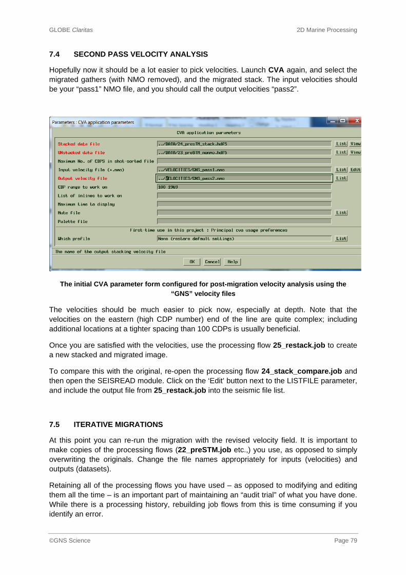
GLOBE Claritas 2D Marine Processing
©GNS Science Page 79
7.4 SECOND PASS VELOCITY ANALYSIS
Hopefully now it should be a lot easier to pick velocities. Launch CVA again, and select the migrated gathers (with NMO removed), and the migrated stack. The input velocities should be your “pass1” NMO file, and you should call the output velocities “pass2”.
The initial CVA parameter form configured for post-migration velocity analysis using the
“GNS” velocity files
The velocities should be much easier to pick now, especially at depth. Note that the velocities on the eastern (high CDP number) end of the line are quite complex; including additional locations at a tighter spacing than 100 CDPs is usually beneficial.
Once you are satisfied with the velocities, use the processing flow 25_restack.job to create a new stacked and migrated image.
To compare this with the original, re-open the processing flow 24_stack_compare.job and then open the SEISREAD module. Click on the ‘Edit’ button next to the LISTFILE parameter, and include the output file from 25_restack.job into the seismic file list.
7.5 ITERATIVE MIGRATIONS
At this point you can re-run the migration with the revised velocity field. It is important to make copies of the processing flows (22_preSTM.job etc.,) you use, as opposed to simply overwriting the originals. Change the file names appropriately for inputs (velocities) and outputs (datasets).
Retaining all of the processing flows you have used – as opposed to modifying and editing them all the time – is an important part of maintaining an “audit trial” of what you have done. While there is a processing history, rebuilding job flows from this is time consuming if you identify an error.

GLOBE Claritas 2D Marine Processing
©GNS Science Page 80
8. FINALISATION
8.1 OBJECTIVES:
Post-stack deconvolution
Random noise attenuation
Filtering
Scaling
SEGY output
8.2 TESTING DECONVOLUTION AFTER STACK
Despite the pre-stack deconvolution that was applied, the migrated section still has some reverberations or short period multiples. We can address these by a further application of deconvolution, using the PSDECON module.
Open the processing flow 26_das.job. This flow reads in a migrated section and applies a series of post-stack deconvolution to repeated copies, using a series of IF and ELSEIF loops. If needed, modify the input file to match your migrated output.
The processing flow 26_DAS.job, which uses IF-ELSEIF-ENDIF to apply different
deconvolution to the migrated dataset with the goal of reducing the reverberations
GLOBE Claritas 2D Marine Processing
©GNS Science Page 81
As with the pre-stack deconvolution, an autocorrelation function has been appended to the stacked section as an aid to picking the best parameters. Run the job, and view the results with and without the AGC.
Try adjusting some of the deconvolution parameters, remembering to update the labels in the PANELTEXT module. In particular, adjusting the design window and gap can have a significant impact.
8.3 RANDOM NOISE ATTENUATION TESTS
GLOBE Claritas™ includes a number of methods for attenuating random noise on a section. These methods use some measure of lateral continuity to define and remove incoherent energy, or use some kind of spatial mixing.
The processing flow 27_random.job applies a number of different techniques to a small panel of data which has had a post-stack deconvolution applied. You should modify the job to include your selected deconvolution parameters and your migration.
The processing flow 27_random.job which tests different random noise attenuation techniques
on stack panels, labelling them using PANELTEXT

GLOBE Claritas 2D Marine Processing
©GNS Science Page 82
Run the flow with and without AGC. The impact of the noise attenuation is quite small in this case, and you may need to use the "plot difference" functions to see the impact clearly. In general, the FXDECON panel tends to have some random noise removed, but still retains a crisp image.
Try modifying some of the parameters. Note that filtering too harshly can remove a lot of the character from a section. You can also add multiple calls to a given technique – such as two FXDECON modules.
8.4 TESTING FILTERS
There is quite a lot of low frequency noise in the dataset, particularly after the deconvolution. In addition, at depth, the high frequencies are unlikely to contain any useful data. The processing flow 28_filter.job applies a deconvolution and random noise attenuation, and then generates a total of ten panels.
The first panel has no filter applied. Panels 2-6 vary the high-cut of the filter. Panels 7-10 vary the low cut of the filter. The filter parameters are controlled by an ASCII “spread sheet” (28_varying.fdf) which changes the filter with each value of the REPEAT trace header configured during SEISREAD.
The processing flow 28_filters.job which tests different filter panels
Open the processing flow and modify the job to read your migration; use your selected deconvolution and random noise attenuation modules.
Run the job. You can create “difference sections” by clicking on the ‘Plot Difference’ option from the ‘Utils’ menu. Note the filters are labelled automatically.
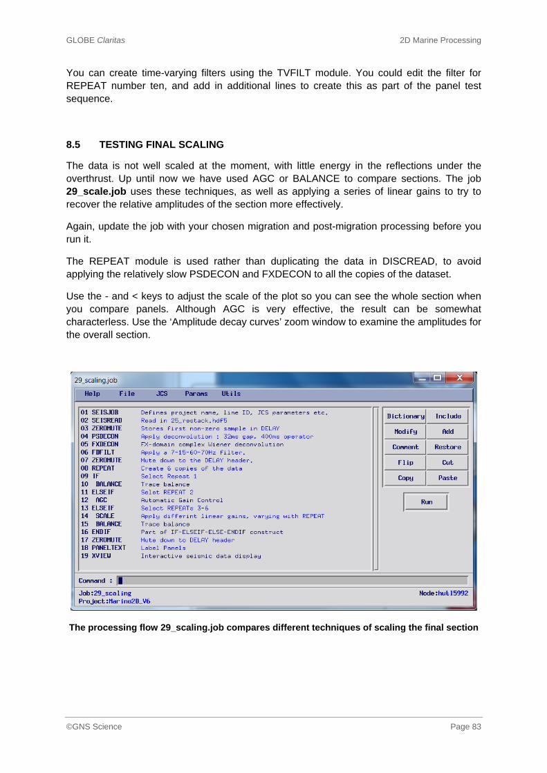
GLOBE Claritas 2D Marine Processing
©GNS Science Page 83
You can create time-varying filters using the TVFILT module. You could edit the filter for REPEAT number ten, and add in additional lines to create this as part of the panel test sequence.
8.5 TESTING FINAL SCALING
The data is not well scaled at the moment, with little energy in the reflections under the overthrust. Up until now we have used AGC or BALANCE to compare sections. The job 29_scale.job uses these techniques, as well as applying a series of linear gains to try to recover the relative amplitudes of the section more effectively.
Again, update the job with your chosen migration and post-migration processing before you run it.
The REPEAT module is used rather than duplicating the data in DISCREAD, to avoid applying the relatively slow PSDECON and FXDECON to all the copies of the dataset.
Use the - and < keys to adjust the scale of the plot so you can see the whole section when you compare panels. Although AGC is very effective, the result can be somewhat characterless. Use the ‘Amplitude decay curves’ zoom window to examine the amplitudes for the overall section.
The processing flow 29_scaling.job compares different techniques of scaling the final section
GLOBE Claritas 2D Marine Processing
©GNS Science Page 84
8.6 FINAL COMPARISON
The processing flow 30_compare.job shows the impact of the finalisation sequence on a migration; update this job to reflect your own choice of parameters. This final section should be a vast improvement over the original near-trace plot and brute stack.
8.7 SEG-Y OUTPUT
The SEG-Y format, defined in 1973 by the Society of Exploration Geophysicists (SEG), is a tape standard for the exchange of seismic data. It is the most common format used for seismic data in the exploration and production industry. The widespread use of 3D data and pre-stack archiving has led to a broad range of modernised varieties of the SEG-Y formats. The actual standards for this and a number of formats can be downloaded from the SEG website (www.seg.org). True SEG-Y is actually quite limited and was designed for storing a single line of seismic data on IBM 9-track tapes, attached to IBM mainframe computers. Most of the differences in modern SEG-Y varieties result from trying to overcome these limitations.
Some of the features of SEG-Y which are outdated today include:
EBCDIC descriptive header (rather than the now-standard ASCII)
IBM floating-point data (rather than the now-standard IEEE)
single line storage (rather than the now-common 3D surveys)
The official standard SEG-Y consists of the following components:
a 3200-byte EBCDIC descriptive reel header record
a 400-byte binary reel header record
trace records consisting of
o a 240-byte binary trace header
o trace data
In true SEG-Y format the information to be placed in the 240-byte header was well defined – although a portion of the header was set up to be user allocated. The 3200-byte text description also had a precise format. In practice, the need to capture a greater level of information in the trace header has led to a more flexible use of the available 240-bytes. Variations from the standard are usually documented in the 3200-byte text header. A “good” SEG-Y file will contain everything you would want to know about the data prior to loading and interpretation. A “bad” file can take many attempts to load.

GLOBE Claritas 2D Marine Processing
©GNS Science Page 85
The processing flow 31_segyout.job is designed to write out a final SEG-Y file, ready for data loading. It also merges the seismic data with the navigation information, so that each trace has a unique Easting and Northing. Navigation data is usually supplied in a UKOOA (UK Offshore Operators Association) P1 text format. In this case, the data is in the P1 format as supplied by the New Zealand Ministry of Economic Development. The P1 file contains the location of each shot as both a latitude/longitude and Easting/Northing pair.
8.7.1 Calculating the CDP to SP Relationship
Because the navigation is based on the shot location, we have to calculate the equivalent shot-point location for each CDP. While GLOBE Claritas™ can extrapolate and interpolate these values, we still need to make sure that this is done correctly. We have shotpoints from 100 to 975, so a total of 876 shots. We also have CDPs from 100 to 1969, or a total of 1870 CDPs. These CDPs include the taper-on at the start of the line and so, although we have two CDPs per shot, there are more than 1752 CDPs. The first live CDP corresponds to data associated with the far offset trace at the first shotpoint. This is positioned halfway between the source and far channel some 1616.5m behind the source: 1616.5m = ((119 channels x 25m separation) + 258m near offset)/2 This in turn corresponds to an additional 64.66 shotpoints (1616.5m/25m) So – the first live CDP is located at the position where shotpoint 34.34 (100-64.66) would have been; this is not a “real” shotpoint number, but an extrapolation of the shotpoint navigation numbers back along the cable. At the far end of the line, the last trace will correspond to the near offset trace from the last seismic shot. This will be positioned half way between the near offset trace and the last shotpoint, so a total of 129m behind the last shotpoint: 129m = (258m near offset) / 2 This corresponds to 5.16 shots – hence the shotpoint location at the last CDP number is
(975-5.16) = 969.84
So the full line range corresponds to shotpoint 34.34 to shotpoint 969.84; these are rounded up to shotpoints 35-970. Open 31_segyout.job and review the modules that are used.
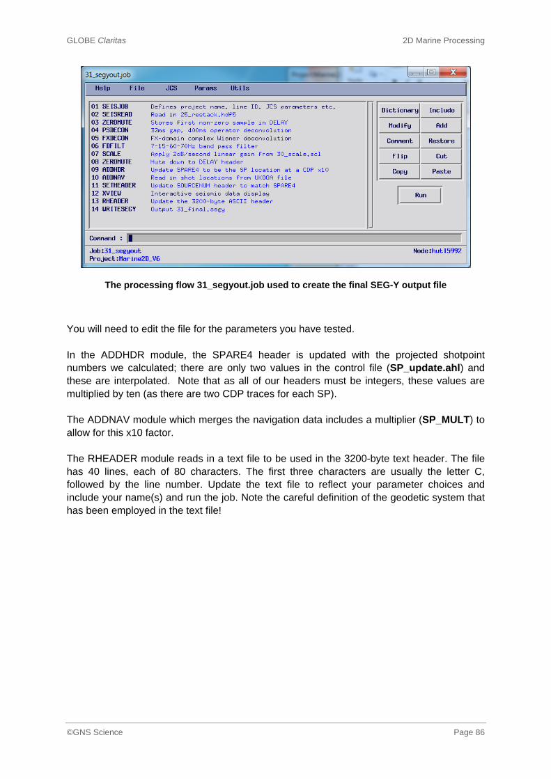
GLOBE Claritas 2D Marine Processing
©GNS Science Page 86
The processing flow 31_segyout.job used to create the final SEG-Y output file
You will need to edit the file for the parameters you have tested. In the ADDHDR module, the SPARE4 header is updated with the projected shotpoint numbers we calculated; there are only two values in the control file (SP_update.ahl) and these are interpolated. Note that as all of our headers must be integers, these values are multiplied by ten (as there are two CDP traces for each SP). The ADDNAV module which merges the navigation data includes a multiplier (SP_MULT) to allow for this x10 factor. The RHEADER module reads in a text file to be used in the 3200-byte text header. The file has 40 lines, each of 80 characters. The first three characters are usually the letter C, followed by the line number. Update the text file to reflect your parameter choices and include your name(s) and run the job. Note the careful definition of the geodetic system that has been employed in the text file!
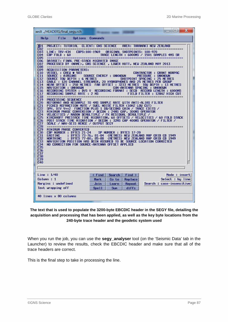
GLOBE Claritas 2D Marine Processing
©GNS Science Page 87
The text that is used to populate the 3200-byte EBCDIC header in the SEGY file, detailing the
acquisition and processing that has been applied, as well as the key byte locations from the
240-byte trace header and the geodetic system used
When you run the job, you can use the segy_analyser tool (on the ‘Seismic Data’ tab in the Launcher) to review the results, check the EBCDIC header and make sure that all of the trace headers are correct. This is the final step to take in processing the line.

GLOBE Claritas 2D Marine Processing
©GNS Science Page 88
APPENDIX 1: LINE TRV434
The data have been reformatted from the original SEGD to GLOBE Claritas™ in-house format (CSEG-Y) and resampled to 4 millisecond sample interval with a 70Hz-80Hz High Cut anti-alias filter applied. This reformatting would normally comprise the first job in the processing sequence (Job1), but it has been applied simply to reduce the size of the dataset. The effects of towing the source and receiver at depth limits the frequency content of the signal (as a result of an effect called “ghosting”, arising from reflected energy from the sea-surface) to a level where frequencies over 80Hz are unlikely to exist; frequencies up to 80Hz can easily be represented at a 4 millisecond sample interval and so no loss of signal results from this process. With a group interval of 25 metres, the “natural” CDP spacing is half of this, or 12.5 metres. The majority of marine seismic data that is collected is processed at a 12.5 metre CDP “bin” spacing. Modern acquisition systems can record many channels and 12.5 metre groups or even finer are becoming common place. In practice, this is not usually done so that the data can be processed with a 6.25 metre or finer CDP spacing, but to let the processor control how the receiver array is to be formed. For example, where 12.5 metre field groups have been used, it is common to combine these and renumber to give 25 metre groups and half the number of channels. If noisy or spiking channels are edited out prior to this array forming process, a whole array will only be blank if both of the channels combined into a single group have been killed. This means there will be fewer dead traces within the shot and CDP gathers, improving the quality of any manual or statistical analysis. In this case, the data will be processed with a 12.5 metre CDP interval. Each CDP will have up to 60 traces from different shots and receivers. Variations in this will occur where there are missing shots or channels, and at the start and end of the line (taper on and taper off), where the number of traces will ramp up from (and down to) 1. The number of traces in a CDP gather is referred to as the fold (sometimes called the multiplicity). This can be expressed as a coverage percentage: single-fold = 100% coverage, sixty-fold = 6000% coverage, and so on.
Fold = (Receiver Spacing x Number of Receivers) / (2 x shot spacing)
Fold = (25 x 120) / (2 x 25) 60
In this case, with a 25 metre shot spacing and 120 receivers, the maximum fold is 60.

GLOBE Claritas 2D Marine Processing
©GNS Science Page 89
APPENDIX 2: MARINE PROCESSING
MARINE PROCESSING OBJECTIVES
When we process 2D marine data, we want to create a fully formed image of the subsurface. In order to do this, a series of sound waves have been created that have spread out through both the water and rock layers. This energy has been scattered and refracted as a result of variations in the physical properties of the rocks. The scattered wave-front that returns to the surface has been sampled and recorded by an array of receivers.
The only energy we are interested in using to form the image is P-wave energy that has the simplest possible reflected path to our receiver array. All other energy is considered to be noise that needs to be attenuated or removed. This includes energy that has reflected off more than one interface or surface, including the surface of the sea, before being recorded.
We also want to try to correct – or at least acknowledge – some of the factors that will cause the nature of the wavefront to change as it propagates through the sub-surface. It will lose energy, both as a result of losses on transmission or reflection, and as a result of spherical spreading. Higher frequencies will be absorbed faster than lower ones, so that a frequency range that contains useful energy in the near surface might only contain noise at depth.
There may also be specific types of environmental noise that need to be addressed. Most commonly, there will be noise that arises through the sea swell, both directly and as a result of the motion it induces in the recording cable. There may also be noise from the engines of the acquisition (or indeed any other) vessel, nearby machinery on a drilling platform, fish bites or impacts on the cable, or even the airgun “shots” from other vessels acquiring data in the same area.
Finally there are factors associated with the equipment that has been used. These included digital spikes in the recording system, array miss-fires, and the fact that our equipment is deployed beneath the surface of the sea and not directly at the surface.
In general, then, all of the processing stages are designed to achieve one (or more) of the following:
• Improve the signal-to-noise ratio, where “noise” is anything that is not a primary reflection.
• Modify, control, and simplify the shape of the seismic wavefront.
• Form an image of the sub-surface structure from the scattered wavefield measured at the surface.
Marine Processing Methodology
In general, a single processing sequence is developed and applied to all of the data within a survey. This methodology works well where the survey is spatially limited since (for the most part) the sub-surface geology varies relatively slowly. Where the geology varies extremely rapidly, such as in areas where there is a lot of folding, faulting or deformation, generating a high quality and accurate seismic image is extremely challenging.
GLOBE Claritas 2D Marine Processing
©GNS Science Page 90
The processing sequence is usually tested on one or more representative subsets of the data, and then applied in stages. This ensures that we can check at regular intervals that the application of the processing flow to the whole data-set has had the desired results, and that no problems or errors have been encountered.
On large projects, this also allows a “production flow” to be developed, so that, for example, one team member pushes through the testing and production on a single seismic line (a test line), and, passes the results of those tests to other team members. They run the rest of the data through the stages that have been fully tested, carefully applying a series of quality control checks to ensure that the sequence has been correctly applied and has had the desired effects.
In some cases, a processing sequence that varies spatially (or to be more accurate, as a result of varying water depth or geology) will be required. Variations on a line-by-line basis can also occur where the acquisition parameters have been modified. Where a varying sequence has to be applied, the quality control checks should be designed to highlight any additional issues as a result of this added complexity.
Processing sequences are always a compromise between solving specific localised problems and having a good general sequence. For example, many processing stages use the spatial continuity of sub-surface reflections to separate signal from random noise, but, depending on the criteria selected to define the “randomness” of the data, can also reject data in regions of geological complexity or steep dip. The selection of both the test line and test areas on that line must take this into account.
This compromise is the reason why many datasets are re-processed at different stages of exploration or investigation. The “least harm” sequence applied to a 2D regional reconnaissance survey covering 40,000 km2 will be somewhat different to that used to best image a specific geological target inside a 400 km2 subset of the same area, since the geological and structural variation in the subset will be smaller.
Processing Terminology: Primary and Secondary Keys
In every seismic processing system, each trace has a number of headers associated with it as identifiers and to carry key information. In GLOBE Claritas™, there is a standard set of headers that take up the first 240 bytes of each trace. The headers are each allocated a name – there is a full list of the names and their common usage in Appendix A of the GLOBE Claritas™ manual. Some of these headers are seldom used, for example the headers used to describe a vibroseis sweep pattern when dealing with marine data, and can be allocated other values.
Users can also define any number of additional headers on top of the 240 bytes, which is used for compatibility with the industry exchange format SEG-Y.
Seismic data is usually grouped in some way, for example into files, shots, CDPs. These are usually referred to as ensembles. In GLOBE Claritas™ the headers that identify the ensemble and the relative position of the trace in an ensemble are referred to as the primary and secondary keys respectively. Care must be taken when updating or modifying a primary or secondary key, to avoid duplicate pairings that may cause problems in the data flow.

GLOBE Claritas 2D Marine Processing
©GNS Science Page 91
The last trace in each ensemble carries a “last trace flag” which allows multi-channel processes to work correctly. A similar flag is set on the last trace in the processing flow, to instruct the job to complete.
Generalised Marine 2D Sequence
In general, a marine processing sequence contains the following stages, although some variations in the exact order of given processes, and their technical descriptions, can be expected. This would typically be applied as 4–6 processing stages, with two interactive velocity analysis sessions.
1. Reformat, resample and edit out bad data.
2. Remove refractions and direct arrivals by muting.
3. Correct for signal amplitude losses from spreading and transmission.
4. Remove swell noise and other environmental problems.
5. Apply deconvolution to reduce reverberations and short-period multiple-reflections.
6. Sort the data by common midpoints1 (CDPs).
7. Pick a rough velocity field for the Normal Moveout Correction.
8. Apply pre-stack imaging: either dip-moveout or pre-stack time migration.
9. Remove “multiple” energy caused by energy reverberating in the water column.
10. Second, accurate velocity analysis.
11. NMO correction and far-offset mute.
12. Stack the data within each CDP.
13. Residual or full migration, depending on the pre-stack imaging applied.
14. Additional deconvolution to remove any remaining reverberation.
15. Random noise attenuation / coherency filtering.
16. Filtering.
17. Scaling and output.
1 CDP stands for Common Depth Point, but is used to describe collecting data together by its Common Midpoint (CMP). Although CMP is a more accurate description, CDP is more widely used. In complex areas, depth imaging techniques are employed which create true common points in depth. These are commonly referred to as Common Reflection Points (CRP) to distinguish them from the (misnamed!) CDP.

GLOBE Claritas 2D Marine Processing
©GNS Science Page 92
APPENDIX 3: USEFUL UNIX COMMANDS
USEFUL COMMANDS
For those with little or no UNIX experience, the following may be useful:
ls Creates a list of the files in a directory.
ls –latr Creates a list of all of the files in a directory, including special files, arranged so that the most recent file is last in the list.
rm filename Deletes (removes) the file called filename. There is NO way to “undelete” the file.
cp original_file new_file Makes a copy of a file. If the new-file is a UNIX path, the copy will have the same name in the new location.
more filename Steps through a text file. Use the space bar to scroll, <CTRL-C> to exit
mv original_file new_file Moves a file to a new location, can also be used to rename a file.
mkdir directory_name Creates a new directory called directory_name
rmdir directory_name Removes a directory called directory_name (it must be empty).
top Shows a display of which processes are using the computers CPU; useful on shared machines to find out what else is running. Use <CTRL-C> to exit.
command & Using the “&” runs the command in the background – you can continue to type at the prompt while the command runs.
fg fg moves a command running in the background to the foreground.
<CTRL>-C Pressing <CTRL> and C stops any command that is running.
<CTRL>-Z Pressing <CTRL> and Z suspends (pauses) any command that is running.
bg Places any suspended command into the background.

GLOBE Claritas 2D Marine Processing
©GNS Science Page 93
cd directory_name Changes the working area to the directory called directory_name
cd .. Moves up on directory in a tree
UNIX Directories, Files and Paths
UNIX stores files in directories. In any directory there are two “special” files, called simply . and .. These are actually reference markers that given the operating system information about the properties of the current directory, and the “parent” directory above it.
Although UNIX files and directories can be called virtually anything, it’s a good idea in general to avoid having spaces (use underscores or hyphens) and some symbols ($%&@/\|+ etc.) – you can use these, but since spaces and symbols can have other meanings in UNIX, referencing files with these names becomes complicated.
If your working area has been set to the same directory that a file is in, you can reference that file just by its name. If the file is in a different directory, you will have to add the path to the file name, which tells the UNIX command you are typing where the file is. A path consists of a list of the directories, separated by a slash (/). The directory path and the file name are also separated by a slash.
A path can be absolute – that is to say it is relative to the highest directory level on the disc, which has no name on the system (and is denoted by a single / ), or relative.
So – if the working directory was:
/home/guym
And I wanted to look at a file called README in the directory called TUTORIAL one “level” below, I could type:
more TUTORIAL/README
more /home/guy/TUTOTIAL/README
And it would have the same effect.
If I was in the TUTORIAL sub-directory, and wanted to copy the README file up one level to /home/guy/ I could type any of the following:
cp /home/guym/TUTORIAL/README /home/guym
cp /home/guym/TUTORIAL/README /home/guym/README
cp README /home/guym
cp README /home/guym/README
cp README ..
cp README ../README
GLOBE Claritas 2D Marine Processing
©GNS Science Page 94
APPENDIX 4: TROUBLESHOOTING
If you find that the example processing flows are not working, this may indicate a problem with your system or the installation. There are, however, a few things to try first.
UPDATING THE JOB FLOWS
GLOBE Claritas™ is regularly updated; this means that new parameters are often added into processing modules at the request of users. Although modules are always “backwards compatible” in terms of how they behave, if you are using a version of the tutorial that came with an older release of GLOBE Claritas™, when you come to run a job, you might get messages telling you a parameter is unrecognised, and you should use the ‘Update’ button in the Command window.
Simply dismiss the Command window and press the ‘Update’ button. The parameter form will be updated to include the new parameters, and you will be informed of the changes that have been made. In some cases, updates will be initialised automatically when you open the processing flow.
MISSING FILES
At various points in the tutorial, you may choose to build your own “production job flows”, based on tests. If you use different naming conventions to those suggested, or place files in different directories, then your jobs will fail. The Command window will usually identify which file is missing and the module, but errors like “File fort.7 missing” indicate the same problem.
Work through the job flow using the ‘View’, ‘List’ and ‘Edit’ buttons to confirm all of the data and support files exist.