going to the extremes - climate & global dynamics · going to the extremes an intercomparison...

GOING TO THE EXTREMES

AN INTERCOMPARISON OF MODEL-SIMULATED HISTORICAL ANDFUTURE CHANGES IN EXTREME EVENTS

CLAUDIA TEBALDI1 KATHARINE HAYHOE2,3 JULIE M. ARBLASTER4,5

and GERALD A. MEEHL4

1Institute for the Study of Society and Environment, National Center for Atmospheric Research(NCAR), PO BOX 3000, Boulder, CO 80301

E-mail: [email protected] of Atmospheric Sciences,University of Illinois at Urbana-Champaign, Urbana,IL

3Department of Geosciences, Texas Tech University,Lubbock, TX4Climate and Global Dynamics Division, NCAR,Boulder, CO

5Bureau of Meteorology Research Centre, Melbourne, Australia

Abstract. Projections of changes in climate extremes are critical to assessing the potential impactsof climate change on human and natural systems. Modeling advances now provide the opportunityof utilizing global general circulation models (GCMs) for projections of extreme temperature andprecipitation indicators. We analyze historical and future simulations of ten such indicators as derivedfrom an ensemble of 9 GCMs contributing to the Fourth Assessment Report of the IntergovernmentalPanel on Climate Change (IPCC-AR4), under a range of emissions scenarios. Our focus is on theconsensus from the GCM ensemble, in terms of direction and significance of the changes, at theglobal average and geographical scale. The climate extremes described by the ten indices rangefrom heat-wave frequency to frost-day occurrence, from dry-spell length to heavy rainfall amounts.Historical trends generally agree with previous observational studies, providing a basic sense ofreliability for the GCM simulations. Individual model projections for the 21st century across thethree scenarios examined are in agreement in showing greater temperature extremes consistent with awarmer climate. For any specific temperature index, minor differences appear in the spatial distributionof the changes across models and across scenarios, while substantial differences appear in the relativemagnitude of the trends under different emissions rates. Depictions of a wetter world and greaterprecipitation intensity emerge unequivocally in the global averages of most of the precipitation indices.However, consensus and significance are less strong when regional patterns are considered. Thisanalysis provides a first overview of projected changes in climate extremes from the IPCC-AR4 modelensemble, and has significant implications with regard to climate projections for impact assessments.

1. Introduction

In recent years, the need for regional-scale projections of climate variables andthresholds that are directly relevant to impacts researchers and stake-holders hasbeen strongly voiced (Hare, 2006). Since the IPCC Third Assessment Report(Houghton et al., 2001), climate change detection and projections of future changeare no longer relegated to global averages and have expanded to include extremes(Hegerl et al., 2004). Substantial progress in both global and regional modeling

Climatic Change (2006)DOI: 10.1007/s10584-006-9051-4 c© Springer 2006

C. TEBALDI ET AL.

at medium to high resolution (Duffy et al., 2003; Govindasamy et al., 2003)1 hasprovided the basis for an increasing number of studies that attempt to characterizeexpected changes at local scales. Recent modeling efforts have also provided uswith the ability to characterize changes in terms of indices with greater relevanceto impacts than the traditional climate model outputs of mean temperature, precip-itation and sea level pressure (e.g., Hayhoe et al., 2004; Meehl and Tebaldi, 2004;Meehl et al., 2004; Meehl et al., 2005a).

A primary concern in estimating impacts from climate change are the potentialchanges in variability and hence extreme events that could accompany global cli-mate change. Extreme events such as heatwaves, heavy rain or snow events anddroughts are responsible for a disproportionately large part of climate-related dam-ages (Kunkel et al., 1999; Easterling et al., 2000; Meehl et al., 2000) and henceare of great concern to the impact community and stakeholders (Katz et al., 2005;Negri et al., 2005). Katz and Brown (1994) first suggested that the sensitivity ofextremes to changes in mean climate may be greater than one would assume fromsimply shifting the location of the climatological distributions. Since then, obser-vations of historical changes as well as future projections confirm that changes inthe distributional tails of climate variables may not occur in proportion to changesin the mean, particularly for precipitation, and may not be symmetric in nature,as demonstrated by differential changes in maximum vs. minimum temperatures(e.g., Kharin and Zwiers, 2005; Robeson, 2004; Tank and Konnen, 2003; Easterlinget al., 2000).

Over the past decade, a number of studies have attempted to identify observedand projected future changes in extreme events. These have employed a rangeof temperature and precipitation data that included return periods (e.g., Ekstromet al., 2005; Semmler and Jacob, 2004; Wehner, 2004); frequency-duration-intensityindices (Adamowski and Bougadis, 2003; Khaliq et al., 2005); multivariate statistics(Bohm et al., 2004; Huth and Pokorna, 2005); and indices based on frequency andvariance (Palmer and Raisanen, 2002; Meehl and Tebaldi, 2004).

The landmark effort by Frich et al. (2002, henceforth F02) was instrumentalin setting the stage for a coordinated effort to identify and monitor indices of ex-treme events, both as observed and simulated. In F02, ten indicators of extremeevents were chosen based on their ability to summarize a wide spectrum of cli-mate extreme characteristics, and their robustness in the face of both measurementand predictive uncertainty.2 Robustness is to be viewed as the result of a trade-offbetween the extreme and therefore infrequent nature of the phenomena describedand the availability in the climate records of enough instances of these phenom-ena to allow a stable estimate of their frequency and intensity. The resulting tenindicators may be seen as “not as extreme” as they could be, given the necessarycriteria of sufficient occurrences over the historical observational period, but it isexactly this quality that leaves open the possibility of using climate model outputfor their computation. Inevitably, because of their finite and still relatively coarse


resolution, climate models are not expected to represent extreme weather eventswith the intensity and frequency comparable to what is observed, particularly forprecipitation-related events (Kiktev et al., 2003; Raisanen and Joelsoon, 2002).Nonetheless, the “less extreme” nature of these indices, together with definitionsinvolving climatologies that are model-specific, justifies application of AOGCMoutput to investigate changes in their behavior, and taking the simulated futurechanges as indicative of what we can expect from future climate extremes.

The goal of this study is to survey the most recent projections of climate extremesprovided by the latest state-of-the-art AOGCMs, as contributed to a common archivehosted by PCMDI3 as part of the activities sponsored by the IPCC leading up toits Fourth Assessment Report. Besides standard fields that are the direct output ofthe model simulations, modeling centers have agreed to compute the ten indicatorsdefined by F02 for the 20th century climate (historical) experiments and as projectedfor a range of future SRES emission scenarios. Thus, our objective here is to analyzethese quantities as provided by the modeling centers. There is some indication thatthe methodology used to calculate at least one of the F02 temperature indices,warm nights, results in a bias in the calculation of 20th century trends (Zhang et al.,2005). However, as the purpose of this study is to examine the trends in the indicesas defined by the IPCC for calculation by the AR4 modeling community, we remainwith the original definition although noting this discrepancy for the purposes of theinterpretation of these results.

This multi-model dataset and consistent representation of the ten extreme in-dices enables us to compare the historical simulation results to the observed trendsreported in F02 and to analyze projected changes within and across models. It isimportant to note that a new study has been recently performed and will soon be-come available (Alexander et al., 2005), updating the F02 analysis into a spatiallycomprehensive and current set of estimates of the observed trends in the ten indi-cators. A more quantitative evaluation of the models’ fidelity in simulating trendsin the 20th century extremes awaits release of that dataset. Here, we cite qualita-tive comparisons with previously published estimates of changes in relevant ex-tremes that provide context for the model projections of future changes of extremes(Table II).

The paper is organized as follows. In Section 2 we briefly describe the tenindicators and their significance. In Section 3 we focus on temperature extremes.We first compare model-simulated historical runs to the observational changespresented in F02 in terms of time series of global and hemispheric averages. Wethen proceed to characterize our confidence in the sign of the future expectedchanges, by comparing the different model results and analysing commonalities anddifferences in the future projections under the range of available SRES scenarios.We then focus on geographical patterns, discussing the model consensus in termsof sign and significance of the projected changes for the end of the 21st century.Section 4 mirrors Section 3, but analyzes the five indicators of precipitation extremes

C. TEBALDI ET AL.

TABLE IThe nine Atmosphere-Ocean General Circulation Models featured in our analysis

ClimateModeling center AOGCM sensitivity (TCR)

National Center for Atmospheric Research (USA) CCSM3 1.46

Meteo-France & Centre National de RecherchesMeteorologiques (France)

CNRM-CM3 1.57

US Dept. of Commerce & National Oceanic andAtmospheric Administration & GeophysicalFluid Dynamics Laboratory (USA)

GFDL-CM2.0 1.60

US Dept. of Commerce & National Oceanic andAtmospheric Administration & GeophysicalFluid Dynamics Laboratory (USA)

GFDL-CM2.1 1.50

Institute for Numerical Mathematics (Russia) INM-CM3 1.57

Center for Climate System Research & NationalInstitute for Environmental Studies & FrontierResearch Center for Global Change (JAPAN)

MIROC3.2(medres) 2.11

Center for Climate System Research & NationalInstitute for Environmental Studies & FrontierResearch Center for Global Change (JAPAN)

MIROC3.2(hires) NA

Department of Energy & National Center forAtmospheric Research (USA)

PCM 1.32

Meteorological Research Institute & JapanMeteorological Agency (Japan)

MRI-CGCM2 0.97

instead. Section 5 gives a brief overview of the geographical changes simulated bythe models over the 20th century, for comparison with the future changes. Section 6summarizes the results.

At the time of writing nine models have provided the ten extremes indicators tothe PCMDI archive (see Table I). Although only a subset of all models that havecontributed to the archive, the preliminary results here described will nonethelessprovide a reasonably representative assessment of what might be expected from thefull ensemble of model simulations. The models with extremes indices currentlyavailable are the DOE/NCAR Parallel Climate Model (PCM; Washington et al.,2000) and Coupled Climate System Model (CCSM3)4, the CCSR MIROC mediumand high resolution models (Hasumi and Emori, 2004)5, INM-CM3 (Diansky et al.,2002), CNRM-CM3,6 GFDL-CM2.0, GFDL-CM2.1 (Delworth et al., 2002; Dixonet al., 2003) and MRI-CGCM2 (Yukimoto et al., 2001). Model grid resolutionsvary from relatively coarser (INMCM3, 5◦ × 4◦) to relatively finer (MIROC hi-res, ∼1.125◦). Model simulations are available for the historical period, as well asfor three future SRES emissions scenarios: A2 (higher), A1B (mid-range) and B1(lower) (Nakicenovic et al., 2000). Projected end-of-21st century carbon emissionsfor these scenarios, driven by variations in underlying assumptions regarding pop-


ulation, technology and energy use, range from 5 GtC/yr for B1 up to 29 GtC/yr forA2. Corresponding atmospheric CO2 concentrations in 2100 lie between ∼500 to∼900 ppm.

Of the nine AOGCMs with F02 extremes indices available, there are multipleensemble members of the climate of the 20th century experiment (20C3M) forfive of the models; four from the PCM, three each from MIROC3.2 (medres),GFDL-CM2.0 and GFDL-CM2.1 and five from MRI-CGCM2.3.2. For the three21st century experiments, multiple member ensembles are utilised from the PCMand MIROC3.2 (medres), with single runs from the remaining models. We aggregateall ensemble members from an individual model into an ensemble average, thusanalysing a total of nine sets of simulations for each experiment (20C3M, SRESA2,SRESA1B and SRESB1). It should be noted that extremes indices were unavailablefor the SRESA2 experiments of CCSM3 and MIROC3.2 (hires) models and theSRESB1 scenario of the MRI-CGCM2.3.2 model. Potential impacts on the resultsdue to these omissions are discussed in later sections.

2. Ten Indicators of Climate Extremes

The indices chosen by F02 are intended to be representative of a wide varietyof climate aspects for both subtropical and extratropical regions. Recent studies(Zhang et al., 2005; Alexander et al., 2005) have pointed out limitations of thesedefinitions due to the choice of fixed thresholds, the use of a limited climatology(arguing that the indices have problematic statistical properties, or are not as robustas initially argued), or more generally, that they are not as relevant as claimed.However, our intent in this study is to document the indices as they were computedand submitted by the various modeling centers to the IPCC-AR4 data archive.Recomputing the indices is both not possible from the data available at the time ofwriting and beyond the scope of this study. Instead, we assess simulated historicaland future projected trends using the original index definitions and compare thesewith historical observed trends as calculated by F02 using the same definitions.

Five indices describe temperature-related extremes:

1. Total number of frost days, defined as the annual total number of days withabsolute minimum temperature below 0◦ C (frost days, or Fd in F02).

2. Intra-annual extreme temperature range, defined as the difference betweenthe highest temperature of the year and the lowest (xtemp range, or ETR inF02).

3. Growing season length, defined as the length of the period between the firstspell of five consecutive days with mean temperature above 5◦ C and the lastsuch spell of the year (growing season, or GSL in F02).

4. Heat wave duration index, defined as the maximum period of at least 5 con-secutive days with maximum temperature higher by at least 5◦ C than the

C. TEBALDI ET AL.

climatological norm for the same calendar day (heat waves, or HWDI inF02).

5. Warm nights, defined as the percentage of times in the year when minimumtemperature is above the 90th percentile of the climatological distribution forthat calendar day (warm nights, or Tn90 in F02).

While frost days and growing season have interesting interpretations only forextratropical (mid to high latitude) regions, describing mainly anomalies in thelength of spring and fall seasons, the rest of the indices apply to all areas of theglobe, sampling anomalies in daytime maxima or night-time minima and in thepersistence of extremely hot days regardless of the lower variance encountered intropical regions. Accordingly, in our analysis we calculated frost days and growingseason only for regions poleward of ±30 ◦ latitude.

Five indices describe precipitation extremes:

1. Number of days with precipitation greater than 10 mm (precip > 10, or R10in F02).

2. Maximum number of consecutive dry days (dry days, or CDD in F02).3. Maximum 5-day precipitation total (5 day precip, or R5d in F02).4. Simple daily intensity index, defined as the annual total precipitation divided

by the number of wet days (precip intensity, or SDII in F02).5. Fraction of total precipitation due to events exceeding the 95th percentile of

the climatological distribution for wet day amounts ( precip > 95th, or R95tin F02).

All indices except dry days measure changes in the intensity of rain. As fordry days, even if its definition is evocative of drought events, we regard it as anindicator of less extreme characteristics in the distribution of precipitation. Droughtconditions are the effect of prolonged and complex sets of conditions, involvingmonths- to years-long precipitation deficits and soil moisture characteristics thatthis simple index cannot represent. Rather, the index may be apt to measure thetendency – already hypothesized – towards longer dry spells separating intensifiedwet events, as suggested by the precipitation indices, and this particular associationmay be in fact more relevant to flood-related vulnerability studies due to heavyrainfall events such as have been observed over the continental U.S. (Kunkel, 2003).

It is clear from these definitions that we are not looking at extremely rare events,for which the computation of significant trends could be a priori hampered by thesmall sample sizes. In this respect, an important condition is that the thresholds forheat waves, warm nights and precip >95th be defined as percentiles of the clima-tologies computed from the same model’s historical run between 1961 and 1990(specifically based on 150 values, according to the definition in F02 that requiresto use a 5-day window around the calendar date for the percentile computations).

With regard to the indices counting exceedances of percentile-based thresholds,and expanding on the caveat mentioned at the beginning of this section, we note the


following. It has been recently demonstrated (Zhang et al., 2005) that the use of alimited climatology introduces biases and discontinuities in the time series of theseindices at the boundaries between in-base and out-of-base periods (which in ourcase are at 1961 and 1990). As already mentioned, recomputing the indices in orderto correct these biases is beyond the scope of our study. On the other hand, giventhe qualitative aspect of our comparisons between observed and simulated trends,and the magnitude of the differences we detect between present and future rates ofchange, we believe these discontinuities are not critically affecting our results.

3. Temperature Extremes

3.1. GLOBAL AND HEMISPHERIC AVERAGES

Observationally-based extreme temperature indices analyzed by F02 were consis-tent with the idea of a general warming of the climate at the end of last century withgreater warm extremes and less cold extremes. Significant trends for the observedglobally averaged station records (mainly covering the northern hemisphere) wereestimated for frost days, xtemp range (both decreasing during the last 5 decadesof the 20th century), and growing season and warm nights (both increasing). Theonly globally averaged temperature index that lacked a significant trend was foundto be heat waves.

F02’s findings are consistent with other region-specific studies that used similartemperature indices for locations as diverse as the Caribbean (Peterson et al., 2002);China and South East Asia (Gong et al., 2004; Ryoo et al., 2004; Zhai et al.,2003; Gao et al., 2002); Oceania (Salinger and Griffiths, 2001); Europe (Prietoet al., 2004; Tank and Konnen, 2003); the Middle East (Nasrallah et al., 2003);and South America (Rusticucci and Barrucand, 2004). Most studies find increasesin minimum temperatures and significant changes at the low (5–10%) and high(90–95%) percentiles of minimum and maximum temperature.

We compute time series of global and hemispheric averages over land massesonly, and, in the case of frost days and growing season, over extra-tropical lati-tudes only, defined as poleward of ±30◦. Linear trends were fitted to the last 40years of the 20th century time series, and, separately, to the entire length of the21st century time series. Significance of the trends was determined through a tra-ditional Student-t test, where the standard deviation of the residuals was estimatedby (Restricted) Maximum Likelihood, after assuming an autocorrelated process offirst order – as supported by exploratory data analysis – superimposed to the lineartrend, thus accounting for temporal correlation in the residuals. The Student-t testwas determined appropriate, after checking the consistency of the distributions ofthe residuals with the Gaussian assumption, a consistency that we find always sat-isfied (i.e. for all combinations of indices/models/scenarios and for global averages

C. TEBALDI ET AL.

as well as northern and southern hemispheres’ averages). This finding is supportedby the law of large numbers: we are considering trends for time series that resultfrom aggregating many gridpoints into global and hemispheric averages, and weexpect the result of this averages to approximate a Gaussian distribution even ifthe individual quantities (i.e. the individual index time series at each grid location)have distributional characteristics that differ significantly from normal.

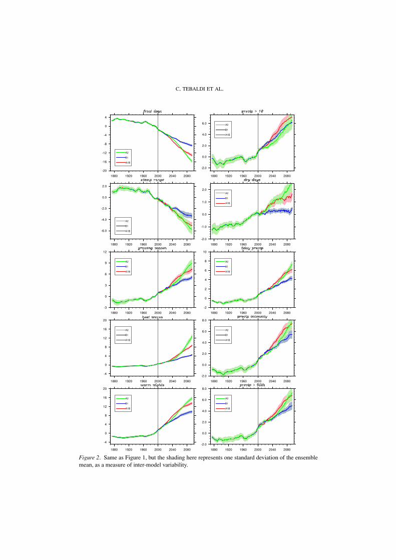
Figures 1 and 2, left column, present multi-model ensemble average time seriesof the temperature indices, globally averaged, and smoothed with a 10-year runningaverage. The time series are the same in both figures. The shadings in Figure 1represent year-to-year variation before the smoothing, while the shadings in Figure 2represent inter-model variability, as one standard deviation of the ensemble average.These summary figures encapsulate the main points highlighted in the followingdiscussion.

When estimating trends over the last 40 years of the 20th century, for global andhemispheric average time series, the nine models easily agree over the sign for allindices but one. The sole exception are the trends estimated for xtemp range over thesouthern hemisphere, with respect to which some models project positive changes,while others project negative changes. These trends, however, are significant fora majority of models only for frost days (decreasing, see first panels of Figures 1and 2, left column) and growing season (increasing, as shown by the third panelsof Figures 1 and 2, left column). Four out of nine models show a significant trendalso for heat waves at the global scale (increasing, as shown in the fourth panelsof Figures 1 and 2, left column), xtemp range (decreasing, see second panels) andwarm nights (increasing, see fifth panels). In comparing the significance of thesetrends with that calculated for observed trends in F02 it is important to note thatestimation of the significance in that study does not seem to take into account thecorrelation in the residuals. This could explain the discrepancy with respect to ourresults: had we simply estimated trends by ordinary least squares, all the indices inall models would show a significant trend in the last four decades of the 20th century,at least at the global level of spatial aggregation. We also note that Kiktev et al.(2003) addressed this issue in their study of six of the ten indices, finding largelyconsistent results with the F02 study, although neither heat waves nor xtemp rangewere included in the subset of indices considered. The results of the comparisonsbetween observed and model-simulated trends over the last 40 years of the 20thcentury are summarized in Table II.

When it comes to future projections, the trends in temperature-related indicesfirst seen over the historical period – even in the cases where they were deemed notsignificant – become stronger and significant in all cases, as clearly shown in allpanels of the left-hand columns in Figures 1 and 2. As in the 20th century, increasesare projected for warm extremes and decreases for cold extremes, consistent withthe general warming in these models associated with increasing greenhouse gasemissions. Common to all simulations is the fact that the trajectories for B1, thelower emissions scenario, separate from (i.e., display a relatively flatter trend than)


Figure 1. Time series of globally averaged (land only) values of temperature (left column) andprecipitation (right column) extremes indices. Three SRES scenarios are shown in different colorsfor the length of the 21st century. The values have been standardized for each model as described inthe main text, then averaged and smoothed by a 10-yr running mean. The envelope of year-to-yearvariation before the 10-yr smoothing is shown as background shading.

C. TEBALDI ET AL.

Figure 2. Same as Figure 1, but the shading here represents one standard deviation of the ensemblemean, as a measure of inter-model variability.


TABLE IISummary of comparisons between observed and simulated trends (1960–2000) at the global averagescale, discussed in Sections 3 and 4

Index Observed trends Simulated trends

Frost days Significant decreasing trend Decreasing trend in all modelsSignificant for a majority(Same for hemispheric averages)

Xtemp range Significant decreasing trend Decreasing trend in all modelsSignificant for four models(SH sees disagreement in sign among models)

Growing season Significant increasing trend Increasing trend in all modelsSignificant for a majority(Trends in SH flat for most models)

Heat waves No significant trend Increasing trend in all modelsSignificant for four models(Same for hemispheric averages)

Warm nights Significant increasing trend Increasing trend in all modelsSignificant for a majority(Same for hemispheric averages)

Precip >10 Significant increasing trend Increasing trend for all modelsSignificant for a minorityHigh inter-annual and inter-model variability

Dry days Significant decreasing trend Increasing trend for all modelsSignificant for a minorityHigh inter-annual and inter-model variability

5 day precip Significant increasing trend Increasing trend for all modelsSignificant for a minorityHigh inter-annual and inter-model variability

Precip intensity No significant trend Increasing trend for all modelsSignificant for a minorityHigh inter-annual and inter-model variability

Precip >95th No significant trend Increasing trend for all modelsSignificant for a minorityHigh inter-annual and inter-model variability

the steeper trajectories of A2 and A1B only well into the 21st century, around2040. This is consistent with estimates of the time of separation in global meantemperature projections under different scenarios due to the lag in climate responseand buildup of CO2 from historical emission patterns (Stott and Kettleborough,2002; Meehl et al., 2005b). The higher emission scenarios A1B and A2 seemto track each other for the greater part of the 21st century in most of the modelsimulations, at a higher rate of increase (for heat waves, warm nights and growingseason) or decrease (xtemp range and frost days) than B1. These higher forcingruns separate only in the latter part of the 21st century, if at all. Results based onthese three scenarios (which can be classified as lower, mid, and mid-high relative

C. TEBALDI ET AL.

to the full SRES range) clearly highlight the influence of emissions scenarios onthe rate of change, suggesting that if this analysis were to be reproduced for an evenlower scenario (e.g., stabilization of GHGs at current-day levels), the projectedtrends would likely diverge even further from the A2 and A1B scenarios than theB1 projections, and show slower rates of increase.

When time series of hemispheric averages are computed for the 21st centurysimulations, warm nights is the only index where the trends in the NH and in theSH have comparable rates of increase. For frost days and growing season the trendsare significant in both hemispheres, but significantly steeper in the NH than in theSH as would be expected given the greater land mass and higher preponderance ofcontinental interiors removed from the moderating effects of the ocean. The sameis true with increasing trends for heat waves. When xtemp range is considered, theSH actually shows either little change (not significant) or even slightly increasingand significant trends (again perhaps reflecting the higher proportion of oceanarea in that hemisphere), but the strongly decreasing and significant trends in theNH prevail in the global average. For the indices characterized by steeper trendsin the NH than in the SH, the separation between scenarios also appears to besharper in the NH than in the SH, especially between the lower-emission B1 andthe higher-emission pair, A2 and A1B. This behavior confirms a more generalconclusion: for quantities showing the steeper trends as a result of anthropogenicforcing, the emission scenarios separate relatively faster and to a greater degreethan for quantities whose rate of change is smaller.

As already noted, Figures 1 and 2, left column, are graphical summaries of theabove discussion, showing multi-model averages of smoothed time series for eachindex and scenario. Each model’s simulated time series of globally averaged valuesfor each index and scenario has been centered with respect to the 1980–1999 pe-riod’s average. Then the standard deviation over the entire 1960–2100 period (afterdetrending) is used to standardize the series before aggregation, in order to adjust fordifferent absolute magnitudes of the simulated indices among the different models(consistent with the general focus of this study on only the direction and significanceof the changes, and the inter-model agreement on those). A 10-year running mean isapplied to smooth the final time series, and the year-to-year variation (in Figure 1)and the ensemble mean’s standard deviation (in Figure 2) are shown as a shading.Hemispheric average time series and single model, non-standardized time seriesare available from http://www.cgd.ucar.edu/ccr/publications/tebaldi-extremes.html.

3.2. GEOGRAPHICAL PATTERNS OF CHANGE

Our analysis at the geographical level focuses on the patterns of change resultingfrom the difference between the average values over the last 20 years of the 21st cen-tury (2080–2099) and the last 20 years of the 20th century (1980–1999). Consistent


with the fact that these indices are mild definitions of extremes and direct deriva-tions of temperature fields, we found that the geographical patterns of changesfor the individual indices across the three SRES scenarios for each model appearto be just modulations of a generally stable geographical pattern of temperaturechange. The pattern of change appears to scale with atmospheric CO2 concentra-tions, such that the pattern obtained under the A2 scenario is a stronger versionof that under A1B, and similarly A1B is a stronger version of what is seen underB1 for that same model. This lends support to projections made using a patternscaling approach (Mitchell, 2003; Watterson and Dix, 2005) and is in agreementwith previous findings that temperature-related impacts and indices tend to scalewith the magnitude of GHG emissions (Hayhoe et al., 2004). In addition, the pri-mary/dominant patterns of change are relatively uniform and robust across the mod-els examined, thus also lending support to the hypothesis that these results will berepresentative, to some degree, of the remainder of the AR4 multi-model AOGCMensemble.

Due to the relatively consistent patterns of geographical change and their appar-ent scaling with CO2 emissions, we next describe the salient features common toall models and without reference to a specific SRES scenario. This is of course ageneralization, but we limit our discussion to the most robust and strongest featuresthat appear to be consistent across all the AOGCMs examined. The significanceof the regional changes was tested by a Student-t test. We computed standarddeviations on the basis of the interannual variability of each of the model/indexcombination over the part of the historical run showing no significant trend (i.e.1900–1949), rescaled by the effective number of observations. For the latter, weperformed an analyisis of the autocorrelation of the gridpoint time series, thusdetermining the lag in years by which subsequent fields generated by the modelfor a specific index simulation can be considered uncorrelated (a lag of one wassufficient in the great majority of cases). Aware of the issue of multiple testingwhen addressing the significance of geographical fields, we set the bar high bydeeming significant only areas where the t-statistics were larger than 3 in absolutevalue (corresponding to an α-level of 0.0025). This, together with the inter-modelconsistency of the patterns, gives us confidence that the regional changes here high-lighted have a high degree of robustness, at least within the current multi-modelensemble.

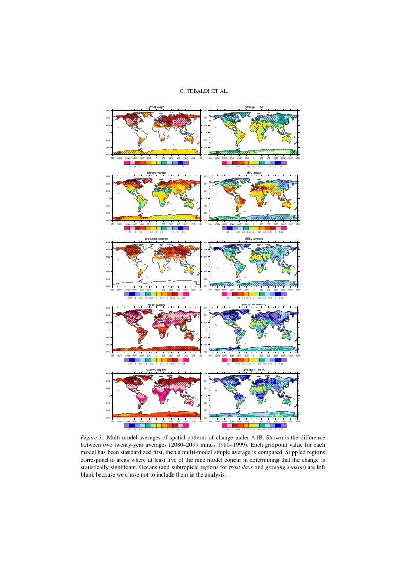
Figure 3, left column, synthesizes our discussion in 5 plots of the geo-graphical changes under the A1B scenario, obtained as a multimodel averagewhere the procedure applied to the time series of Figure 1 is applied grid-point by gridpoint. These should then be considered only qualitative depictionof regional changes as they appear from the aggregation of the single-modelsresults after the model-specific magnitude of the changes has been standard-ized. The dotted regions highlights areas where at least five models in theensemble show a significant change according to the Student-t test at the α-level of 0.0025. A series of model- and scenario-specific geographical plots

C. TEBALDI ET AL.

Figure 3. Multi-model averages of spatial patterns of change under A1B. Shown is the differencebetween two twenty-year averages (2080–2099 minus 1980–1999). Each gridpoint value for eachmodel has been standardized first, then a multi-model simple average is computed. Stippled regionscorrespond to areas where at least five of the nine model concur in determining that the change isstatistically significant. Oceans (and subtropical regions for frost days and growing season) are leftblank because we chose not to include them in the analysis.


are available from http://www.cgd.ucar.edu/ccr/publications/tebaldi-extremes.html.

Frost days patterns (first panel, left column of Figure 3) follow the results de-scribed in Meehl et al. (2004), with a stronger decrease over the high latitudes ofNorth America, propagating southward along the western edge of the continent.Thus, a negative gradient North to South and West to East characterize this indexchange over North America. For Europe and Asia the decrease is weaker along theAtlantic and Mediterranean coasts. The largest decreases are in the Scandinavianregions, and in most models following the topography of the higher elevations ofCentral Asia and Tibet. The North-Eastern part of Asia shows a less substantialdecrease. The southern tips of South America and Africa see the largest decreasescompared to other areas of those continents, consistent with the patterns of changein global mean temperatures which are greater at higher latitudes. The same appliesto the southern latitudes of Australia. All the extratropical regions for which thisindex has a meaningful application see significant decreases by the end of the 21stcentury. As noted by Meehl et al. (2004), the pattern of these changes relates tothe fact that decreases of frost days will be greater near the climatological meanposition of the 0C isotherm, such that small changes near this boundary will resultin relatively greater decreases in frost days in those regions. At higher latitudes,temperatures will continue to go below freezing irregardless of the warming suchthat nighttime temperatures still consistently go below freezing. Greater decreasesof frost days along the western margins of the continents are related to changes inatmospheric circulation, with more warm moist westerly inflow from the oceansin the warmer climate producing relatively greater decreases of frost days in theseregions (Meehl et al., 2004).

Xtemp range patterns (second panel, left column of Figure 3) show changes ofboth signs, despite the fact that the globally averaged index shows a significantdownward trend consistent with greater increases in nighttime minima comparedto daytime maxima found in other models but with spatial differences among mod-els (e.g. Cubasch et al., 2001). Negative changes are consistently simulated overthe higher latitude regions of the northern hemisphere. However, models show aconsistent positive change over the South East U.S. and the Mediterranean basin,up to the mid-latitude regions of Europe. The regions of the southern hemisphereshow mixed patterns, with large regions of positive changes, especially in most ofSouth America, South Africa and Australia. Even if consistently simulated acrossmodels, the individual significance of these changes is less uniform than for theother indices. The majority of models deems significant the negative changes overthe high latitudes of the northern hemisphere and a number of smaller regions in thelower latitudes and the southern hemisphere, characterized by positive changes. Amore complete understanding of these changes would require a detailed analysis ofchanges in diurnal temperature range and the multiple processes affecting patternsof those changes. This is beyond the scope of this paper, but will be addressed in asubsequent study.

C. TEBALDI ET AL.

For growing season (third panel, left column of Figure 3) the significant pat-terns are opposite in sign to the changes in frost days, if somewhat less pronounced,modulating a general increase of the index over all the land masses. Over the U.S.a “belt” of relatively larger values, consistent across all models, appears over theNorthwest, following the Pacific coast and then along the southern regions to theAtlantic coast. This pattern is clearly related qualitatively to the pattern of changesin frost days noted above, even if changes in night-time minima are not the onlyfactor affecting changes in growing season length. For similar reasons, relativelylarger values of the change are also simulated over Eastern Europe, the higher el-evation regions of Central Asia, the southern tip of South America, and southeastAustralia. With regard to the latter, it was pointed out however in F02 that thetemperature-based index is not as relevant for areas such as the Australian con-tinent, where the mild climate puts a larger relevance on precipitation amountsrather than temperature in determining the length and timing of the growing sea-son. The changes simulated are all significant for the mid- and high latitudes ofthe northern hemisphere, but less consistently so across models in the southernhemisphere.

For heat waves (fourth panel, left column of Figure 3), a general significantincrease over the land masses is also observed with large positive values over thesouthwest U.S., a finding that is supported by other recent studies (Hayhoe et al.,2004a,b; Meehl and Tebaldi, 2004). These changes are related to large mean temper-ature increases over land areas, with elements of the pattern associated with changesin atmospheric circulation with increased GHGs (Meehl and Tebaldi, 2004). Otherpatterns consistent across models are a relatively larger increase over North and cen-tral Australia and the high latitudes of the Asian continent, also related to changes inmean temperature outlined in other studies (e.g. Meehl et al., 2005b). The patternsover the West European and Mediterranean regions and Africa are not as consistentwithin the ensemble, with some models placing an area of large intensification overnorthern Europe and others expanding it all the way down to the Mediterraneanbasin and Balcans (consistent with similar findings by Meehl and Tebaldi, 2004).

The values of the change in warm nights (fifth panel, left column of Figure 3)are consistently positive and significant all over the globe, with generally anequator-to-poles negative gradient that is particularly pronounced in the southernhemisphere.

4. Precipitation Extremes

4.1. GLOBAL AND HEMISPHERIC AVERAGES

The analysis of observed historical changes in precipitation extremes indicatorsby F02 produced a picture of a world with intensifying precipitation events,even in the presence of less coherent spatial patterns – when compared to the


temperature-related indicators – as a consequence of the small-scale, local charac-ter of precipitation.

The indices showing the largest, most significant and spatially coherent changeswere found in F02 to be precip >10 and 5 day precip, both indicators of intensifyingprecipitation. That is, for a given precipitation event, proportionately more precip-itation was recorded to fall in a warmer climate. This change is consistent withwarmer oceans evaporating greater amounts of moisture, and the warmer air beingable to hold more moisture. When this moister air moves over land, more intenseprecipitation is produced (Meehl et al., 2005a). A significant trend downward wasfound in dry days, describing a tendency towards less extended dry periods (i.e.more frequent rain events). The trends over the latter part of the 20th century forprecip intensity and precip >95th, were not significant, but their sign too pointedin the direction of a wetter (and more extremely so) global climate.

A number of other studies have found changes in precipitation-related indicesaround the globe that vary by location. For example, Kiktev et al. (2003) foundno change in 5 day precip but some increases in precip >95th and decreasesin dry days. Other studies found increases in heavy rainfall events as measuredby decreasing return periods or increasing rainfall intensity in the western U.S.(Kim, 2005), the Caribbean (Peterson et al., 2002), the U.K. (Fowler and Kisbey,2003), and Italy (Brunetti et al., 2004). However, in contrast to projected changes intemperature extremes, observed precipitation changes were found to exhibit stronglocal to regional-scale variability (e.g., U.K. – Ekstrom et al., 2005; New Zealand-Salinger and Griffiths, 2001; South East Asia – Manton et al., 2001).

The ensemble average time series summarizing our findings can be seen inFigures 1 and 2, right columns. The model simulations for the last 40 years ofthe 20th century are consistent with the findings in F02 with regard to the sign ofthe trends where the intensification of precipitation is concerned. The four indicesmeasuring the intensity of rainfall events, precip >10 (first panels, right column ofFigures 1 and 2) 5 day precip (third panels), precip intensity (fourth panels) andprecip >95th (fifth panels), all show positive trends in the aggregated time series,even if individual index/model combinations may not deem the trend significant,due to the large year-to-year variability of the global and hemispheric means. Thus,the intermodel spread around the ensemble average of these indices appears large,as can be assessed from the shading in Figure 2. For dry days (second panels,right column of Figures 1 and 2) the model average shows an increasing trend,contrary to the observed records, but the inter-model variability and the interannualvariability are large for this index as well.

When it comes to future projections over the entire 21st century, the modelsdo agree on both the positive sign and the significance of the trends for all of theindices measuring rainfall intensity, as clearly shown in the corresponding panels ofFigures 1 and 2 – although whether this is a reflection of greater scientific certaintyor merely similar assumptions underlying the physical parameterizations of themodels examined remains to be seen. Nonetheless, this is physically consistent

C. TEBALDI ET AL.

with the warmer air in the future climate being able to hold more moisture. Theincreasing trends of the wet indices all show a larger positive slope in the courseof the 21st century simulations, compared to the trend observed in the last part ofthe 20th century in association with the greater increases of temperature and thusincreased moisture-holding capacity of the air. For dry days (second panels of theright columns in Figures 1 and 2) the majority of models continue to project a flatglobal and hemispheric average trend for the lowest emission scenario, B1 (with theexception of the GFDL models, predicting a significant increase), while significantincreases are predicted under A2 and A1B.

Compared to the temperature indices, the separation of the trajectories of agiven precipitation index under the different scenarios appears less cleanly, as aconsequence of higher inter-model and interannual variability. It should also benoted that the steepness of the 21st century trends in the precipitation indicesdoes not always scale with the strength of the emissions, i.e. the A1B precipi-tation index exhibits a stronger trend than the A2 index. This could in part beattributable to the smaller number of A2 than A1B experiments in the modelensemble. In particular, MIROC3.2 (hires) exhibits the strongest trends in mostof the precipitation indices under A1B, and CCSM3 exhibits the strongest trendfor precip >10 under A1B, and neither model provided indices from the A2experiment.

Table II presents a summary of the comparisons of observational-based trendestimates with historical model simulations.

When considering northern and southern hemispheres separately, generally theprecipitation-indices trends appear of consistent sign, and most often of not signif-icantly different slopes. Hemispheric average time series and single model, non-standardized time series are available from http://www.cgd.ucar.edu/ccr/publications/ tebaldi-extremes.html.

4.2. GEOGRAPHICAL PATTERNS OF CHANGE

Figure 3, right column, shows graphical summaries for the five precipitation indicesof the geographical patterns of change and the multi-model consensus over theirsignificance. The full spectrum of model- and scenario-specific geographical plotsare available from http://www.cgd.ucar.edu/ ccr/publications/tebaldi-extremes.html.

There is no a priori reason to assume that different emission scenarios willresult in scalable precipitation extremes. On the other hand, results from a study ofaverage precipitation under different scenarios that applied pattern scaling (Tebaldiet al., 2002) found very good agreement among geographical patterns of averageprecipitation change under SRES A2, A1B and B2.

In fact, we also find that for the five precipitation indices, as for the temperatureindices, the geographical patterns of change between the last 20 years of the 20th


century and the last 20 years of the 21st century do appear similar across scenariosalthough they do not always increase in magnitude with emissions, suggesting per-haps that they are more a function of model dynamics and parameterization and howthe model responds to forcing than to emission scenarios per se. Intensification ofthe rainfall amounts, as measured by 5 day precip, precip intensity and precip >95th(third, fourth and fifth panels, right column of Figure 3) produces positive changesover all the land masses. These changes are deemed significant by a majority ofmodels across the mid- to high latitudes of the northern hemisphere and the tropi-cal regions of South America and Africa. Reasons for this pattern are likely relatedto two factors: (1) proportionately more precipitation and precipitation intensityin areas of existing storm tracks and associated dynamical moisture convergenceresulting simply from the greater moisture holding capacity of the warmer air, and(2) a slight poleward shift of the midlatitude storm tracks (e.g. Meehl et al., 2005a;Yin, 2005).

Coherent patterns emerge from the multi-model average for precip >10 and drydays (first and second panel of Figure 3), but the significance of these changes ismuch less uniform than for the other indices. The nine models show large areasof both negative and positive change. The mid- and high latitudes of the northernhemisphere see an increase in precip >10 and at the same time a shortening, on av-erage, of the length of the dry spells. The lower latitudes of the northern hemisphereand the southern hemisphere see a tendency towards longer dry spells, associatedto changes in precip >10 of both signs, the latter not consistent across models. Theregions of significant change in either indices by a majority of models are very fewand have a finer scale than the ones highlighted for the other precipitation indices.Low latitudes and southern hemisphere in general are areas where mean rainfall isprojected as decreasing across the models (Meehl et al., 2005a). Thus, even thoughprecipitation intensity increases in those regions, there are longer periods betweenrainfall events (more consecutive dry days) and a decrease in average rainfall. Inother words, it rains less frequently, but when it does rain, there is more precipitationfor a given event.

5. Twentieth Century Geography of Change in Simulations

Figure 4 shows geographical patterns of changes computed as standardized differ-ences between 1980–1999 and 1900–1919 to provide a comparison of these spatialchanges with the changes computed for the future.

For all the indices it is clear that the dominant patterns surfacing with significantstrength at the end of the 21st century are the ones already present at the end of the20th century. This is – not surprisingly – most evident in the temperature-relatedindices (left columns of Figures 3 and 4), but is detectable in the precipitationindices as well.

C. TEBALDI ET AL.

Figure 4. Multi-model averages of spatial patterns of change at the end of the 20th century. Shownis the difference between two twenty-year averages (1980–1999 minus 1900–1919). Each gridpointvalue for each model has been standardized first, then a multi-model simple average is computed.Stippled regions correspond to areas where at least five of the nine model concur in determiningthat the change is statistically significant. Oceans (and subtropical regions for frost days and growingseason) are left blank because we chose not to include them in the analysis.


With regard to the spatial coherence and the significance of these changes, ourfindings are consistent with what we have already discussed in this paper, and whatF02 and Alexander et al. (2005) show on the basis of the observational data sets.Temperature indices show larger coherent areas of change, and of larger statisticalsignificance than the precipitation indices. The stippling in Figure 4 shows areaswhere a majority of models have simulated statistically significant changes. Herewe apply the same Student-t test that we applied to test significance for the changesat the end of the 21st century, depicted in Figure 3, but we lower the threshold to twostandard deviations rather than three, thus to a nominal α-level of 0.05. The indicesassociated with changes in minimum temperature, frost days and warm nights andthe heat wave index (first, fifth and fourth panels, left column of Figure 4) showwide consensus in the significance of the changes over most of the land areas,while growing season and Xtemp range see more limited areas of significance. TheXtemp range index is unique among the temperature indices in showing changes ofboth signs (even if the models do not attribute statistical significance to the positivechanges), this fact too consistent with the projected changes over the 21st century.

None of the precipitation indices (right column of Figure 4) shows significantregions of change, even at this lower level of statistical significance. Nonethelessthe patterns of change do represent a “preview” of what is in store for the nextcentury, hinting at the fact that although the trend is still confounded by year-to-yearvariability and the inter-model spread, it is arguably already in existence.

6. Conclusions

When considering the simulation of extreme climate we do not yet expect modelsto accurately reproduce observed absolute quantities or rates of change: on the oneside the still relatively coarse resolution of AOGCMs prevents the simulation ofphenomena that manifest their intensity mainly at synoptic scales; on the other side,if we wanted to aggregate locally recorded extreme events over the typical modelgridbox, arbitrary choices of aggregation and interpolation would be necessary.Thus, in this study, we did not analyse the agreement (both among models andcompared to observed data) of model-simulated absolute values. This awaits therelease of the new gridded observational extremes product by Alexander et al.(2005). Rather, our goal consisted primarily of determining if results from differentclimate model simulations can support general statements in terms of tendenciesfor the future climate, and if they are physically consistent with what we wouldexpect to occur given the processes known to be relatively well-simulated in themodels. Thus, we chose to evaluate the sign of current (defined as the last 40 yearsof the last century) and future (over the entire 21st century) trends, and geographicalpatterns of change (defined as the difference between the last 20 years of 20th and21st centuries), focusing on statistical significance of the sign of change, agreementwith observed tendencies and inter-model agreement.

C. TEBALDI ET AL.

Our analysis enables a number of conclusions to be drawn, namely:

– Models agree well with observations that there has already been a trend intemperature-related extremes in the positive direction for growing season,heat waves and warm nights and in the negative direction for frost days, andxtemp range – the latter at least at the global scale of aggregation, dominatedby the behavior of the index in the northern hemisphere – consistent with thenotion of a warming climate.

– Over the next century, all models show a continued trend for more extremesin the temperature-related extremes indices. This trend is of the same sign butgreater magnitude than observed over the past century, and again is consistentwith a warming climate due mainly to increases of anthropogenic GHGs.

– Projected geographical changes in temperature extremes are relatively con-sistent across models and appear to scale with emissions scenario (demon-strating a strong relationship between GHG emissions and the magnitude ofpotential impacts as reflected by the temperature indices). In particular, “hotspots” include the following:

• The high latitudes of the northern hemisphere for most of these indices, asa general consequence of the higher rate of warming already documentedin many studies of climate change. In particular for xtemp range the largestsignificant negative changes are concentrated over these areas.

• The northwest region of North America, particularly for decreases infrost days and increases in growing season length and the Southwest forincreasing incidence of heat waves, related mainly to changes in atmo-spheric circulation with increasing GHGs.

• Eastern Europe for the larger increases in growing season and decreasesin frost days over that continent, again related mainly to changes in atmo-spheric circulation.

• Northern Australia for the largest increases in heat waves over that con-tinent, and Australia’s South East for the largest changes in frost days(decreasing) and growing season (increasing).

– Models also agree with observations over the historical period that there isa trend towards a world characterized by intensified precipitation, with agreater frequency of heavy-precipitation and high-quantile events, althoughwith substantial geographical variability.

– The high latitudes of the northern hemisphere show the most coherent re-gional patterns of significant positive changes in the intensity of wet events,defined through four of the precipitation extremes indices: precip >10, 5 dayprecip, precip >95th and precip intensity. These changes are related to thegreater moisture-holding capacity of the warmer air contributing to greatermoisture convergence, as well as a poleward shift of the storm tracks.


– The index intended to measure dry spell duration, dry days, shows a posi-tive global trend in future projections only for the higher emission scenarios,B1 producing a flat time series for the index in the future. This is the indexshowing the largest relative interannual and inter-model variability. Regionalpatterns seem to differentiate high latitudes of the northern hemisphere, wherenegative changes are consistently predicted even if the significance remainsat best spotty, to the lower subtropical latitudes of the same hemisphere, andthe southern hemisphere, where positive changes predominate. However, asnoted previously, the dry days index is not adequate to capture the kind ofsustained drought conditions that would have severe impacts on water avail-ability for most human systems. For this reason, this index is perhaps moreuseful to complement the precip >10, 5 day precip, precip >95th and pre-cip intensity indices in identifying changes in the proportion of wet and drydays and the distribution of rainfall. Taken together, these five indices of-fer a picture of regions whereby little to no change in mean precipitationcould mask a simultaneous increase in both dry day periods and heavy rain-fall events conducive to flooding conditions (Kunkel, 2003; Kunkel et al.,1999).

Estimates of changes in temperature and precipitation extremes, as presentedhere, are of key importance to assessments of the potential impacts of climatechange on human and natural systems. In the past, such assessments have often hadto depend on projected changes in climate means (USGCRP, 2000) despite the factthat it is the climate extremes that currently cause the most weather-related damages(Kunkel et al., 1999; Easterling et al., 2000; Meehl et al., 2000). In the future, risingfrequency, intensity and duration of temperature extremes – both individual days,as represented by warm nights, as well as extended periods of extreme heat, asrepresented by heat waves – are likely to have adverse effects on human mortalityand morbidity (McMichael and Githeko, 2001). Changes in precipitation-relatedextremes such as heavy rainfall and associated flooding also have the potentialto incur significant economic losses and fatalities (Kunkel et al., 1999). Naturalsystems will likely be affected by changes in both temperature and precipitationextremes, as these have been shown to cause shifts in ecosystem distributions,trigger extinctions, and alter species morphology and behaviour (Parmesan et al.,2000).

Estimating future potential changes in both temperature and precipitation ex-tremes provides essential input to urban, regional and national adaptation and plan-ning strategies through the establishment of, for example, heat watch-warning sys-tems or flood prevention strategies (e.g., Sheridan and Kalkstein, 2004; Hawkeset al., 2003). Our hope is that the analysis presented here, which attempts tohighlight both areas of agreement as well as uncertainty, contributes to thiseffort.

C. TEBALDI ET AL.

Acknowledgements

We acknowledge the international modeling groups for providing their data foranalysis, the Program for Climate Model Diagnosis and Intercomparison (PCMDI)for collecting and archiving the model data, the JSC/CLIVAR Working Group onCoupled Modelling (WGCM) and their Coupled Model Intercomparison Project(CMIP) and Climate Simulation Panel for organizing the model data analysis ac-tivity, and the IPCC WG1 TSU for technical support. The IPCC Data Archive atLawrence Livermore National Laboratory is supported by the Office of Science,U.S. Department of Energy. Portions of this study were supported by the Office ofBiological and Environmental Research, U.S. Department of Energy, as part of itsClimate Change Prediction Program, and the National Center for Atmospheric Re-search. This work was also supported in part by the Weather and Climate Impact As-sessment Initiative at the National Center for Atmospheric Research. The NationalCenter for Atmospheric Research is sponsored by the National Science Foundation.Katharine Hayhoe was partially supported by the United States Environmental Pro-tection Agency through Science to Achieve Results (STAR) Cooperative Agreementno. R-82940201, at the University of Chicago, Center for Integrating Statistical andEnvironmental Science. The authors thank Dr. Gabi Hegerl and two anonymousreviewers for their positive and constructive feedback.

Notes

1. See Johns et al., 2004 for a model description and analysis of preliminary experimentswith HadGEM1 for the IPCC Forth Assessment Report, available online at http://www.metoffice.com/research/hadleycentre/pubs/HCTN/HCTN55.pdf

2. Although a low correlation between the chosen indices is also desirable in order to elevate theindividual relevance of each index, to our knowledge no assessment has yet been performed of thecorrelation (or lack thereof) between the ten F02 indices. In terms of temperature, some correlationis inevitable regardless of the type of index chosen in that all indices reflect a warming climate. F02find similar patterns of spatial change for all temperature indices, while both historical observed(F02) and future modelled indices (this study) indicate consistent changes in temperature indicesindicative of an overall warmer climate. For precipitation, much more mixed results are seen,suggesting an overall lower correlation between the individual indices as well as between themodels and observations.

3. The PCMDI archive is accessed through http://www-pcmdi.llnl.gov4. Publications related to CCSM3 are available at http://www.ccsm.ucar.edu/

publications/5. Documentation is online at http://www.ccsr.u-tokyo.ac.jp/kyosei/

hasumi/MIROC/tech-repo.pdf6. Documentation is available through http://www-pcmdi.llnl.gov

References

Adamowski, K. and Bougadis, J.: 2003, ‘Detection of trends in annual extreme rainfall’, Hydro. Proc.17, 3547–3560.


Alexander, L.V., Zhang, X., Peterson, T.C., Caesar, J., Gleason, B. et al.: 2005, ‘Global observedchanges in daily climate extremes of temperature and precipitation’, Submitted.

Bohm, U., Kucken, M., Hauffe, D., Gerstengarbe, F., Werner, P. et al.: 2004, ‘Reliability of regionalclimate model simulations of extremes and of long-term climate’, Nat. Haz. & Earth Sys. Sci. 4,417–431.

Brunetti, M., Buffoni, L., Mangianti, F., Maugeri M., and Nanni, T.: 2004, ‘Temperature, precipitationand extreme events during the last century in Italy’, Global & Planet. Change 40, 141–149.

Delworth, T. L., Stouffer R., Dixon R. et al.: 2002, ‘Review of simulations of climate variability andchange with the GFDL R30 coupled climate model’, Clim. Dyn. 19, 555–574.

Diansky, N. A. and Volodin, E. M.: 2002, ‘Simulation of present-day climate with a coupledatmosphere-ocean general circulation model’, Izvestiya 38, 732–747.

Dixon, K. W., Delworth, T., Knutson, T., Spelman M., and Stouffer, R.: 2003, ‘A comparison ofclimate change simulations produced by two GFDL coupled climate models’, Global & Planet.Change 37, 81–102.

Duffy, P. B., Govindasamy, B., Iorio, J. P., Milovich, J., Sperber, K. R., Taylor, K. E.,Wehner M.F., and Thompson, S. L.: 2003, ‘High-resolution simulations of global climate, part 1: Presentclimate’, Clim. Dyn. 21, 371–390.

Easterling, D. R., Meehl, G. A., Parmesan, C., Changnon, S. A., Karl, T. R., and Mearns, L. O.: 2000,‘Climate extremes: Observations, modeling, and impacts’, Science 289, 2068–2074.

Ekstrom, M., Fowler, H., Kilsby, C., and Jones, P. D.: 2005, ‘New estimates of future changes inextreme rainfall across the UK using regional climate model integrations. 2. Future estimates anduse in impact studies’, J. Hydrology 300, 234–251.

Fowler, H. J. and Kilsby, C. G.: 2003, ‘A regional frequency analysis of United Kingdom extremerainfall from 1961 to 2000’, Intl. J. Clim. 23, 1313–1334.

Frich, P., Alexander, L. V., Della-Marta, P., Gleason, B., Haylock, M., Tank, A. M. G. K. and Peterson,T.: 2002, ‘Observed coherent changes in climatic extremes during the second half of the twentiethcentury’, Clim. Res. 19, 193–212.

Gao, X. J., Zhao, Z. C. and Giorgi, F.: 2002, ‘Changes of extreme events in regional climate simulationsover East Asia’, Adv. Atmos. Sci. 19, 927–942.

Gong, D. Y., Pan, Y. Z. and Wang, J. A.: 2004, ‘Changes in extreme daily mean temperatures insummer in eastern China during 1955–2000’, Theor. & Appl. Clim. 77, 25–37.

Govindasamy, B., Duffy, P. B. and Coquard, J.: 2003, ‘High-resolution simulations of global climate,part 2: Effects of increased greenhouse cases’, Clim. Dyn. 21, 391–404.

Hare, B. (ed.): 2006, ‘Key vulnerable regions and climate change’, in Proceedings of the InternationalSymposium on ‘Key Vulnerable Regions and Climate Change: Identifying Thresholds for Impactsand Adaptation in Relation to Article 2 of the UNFCC’, in press.

Hawkes P., Surendran S., and Richardson, D.: 2003, ‘Use of UKCIP02 climate-change scenarios inflood and coastal defence’, J. Chart. Inst. Water & Env. Mgmt. 17, 214–219.

Hayhoe, K., Cayan, D., Field, C., Frumhoff, P., Maurer, E. et al.: 2004, ‘Emissions pathways, climatechange, and impacts on California’, PNAS 101, 12422–12427.

Hegerl, G. C., Zwiers, F., Kharin, S., and Stott, P.: 2004, ‘Detectability of anthropogenic changes intemperature and precipitation extremes’, J. Clim. 17, 3683–3700.

Houghton, J. T., Ding, Y., Griggs, D. J., Noguer, M., van der Linden, P. J., Dai, X., Maskell, K.,and Johnson, C. A. (eds.): 2001, Climate Change: The Scientific Basis. Contributions of WorkingGroup 1 to the Third Assessment Report of the Intergovernmental Panel on Climate Change.Cambridge University Press, Cambridge and New York, 881 pp.

Huth, R. and Pokorna, L.: 2005, ‘Simultaneous analysis of climatic trends in multiple variables: Anexample of application of multivariate statistical methods’, Intl. J. Clim. 25, 469–484.

Katz, R. W. and Brown, B. G.: 1994, ‘Sensitivity of extreme events to climate change – The case ofautocorrelated time-series’, Environmetrics 5, 451–462.

C. TEBALDI ET AL.

Katz, R., Brush, G., and Parlange, M.: 2005, ‘Statistics of extremes: Modeling ecological distur-bances’, Ecology 86, 1124–1134.

Khaliq, M. N., St-Hilaire, A., Ouarda T., and Bobee, B.: 2005, ‘Frequency analysis and temporalpattern of occurrences of southern Quebec heatwaves’, Intl. J. Clim. 25, 485–504.

Kharin, V. and Zwiers, F.: 2005, ‘Estimating extremes in transient climate change simulations’, J.Clim. 18, 1156–1173.

Kiktev, D., Sexton, D., Alexander, L., and Folland, C.: 2003, ‘Comparison of modeled and observedtrends in indices of daily climate extremes’, J. Clim. 16, 3560–3571.

Kim, J.: 2005, ‘A projection of the effects of the climate change induced by increased CO2 on extremehydrologic events in the western US’, Clim. Ch. 68, 153–168.

Kunkel, K. E.: 2003, ‘North American trends in extreme precipitation’, Natural Hazards 29, 291–305.Kunkel, K. E., Pielke R. Jr. and Changnon, S. A.: 1999, ‘Temporal fluctuations in weather and climate

extremes that cause economic and human health impacts: A review’, Bull. Am. Met. Soc. 80,1077–1098.

Manton, M. J., Della-Marta, P., Haylock, M., Hennessy, K., Nicholls, N. et al.: 2001, ‘Trends inextreme daily rainfall and temperature in Southeast Asia and the South Pacific: 1961–1998’, Intl.J. Clim. 21, 269–284.

McMichael, A. and Githeko, A.: 2001, ‘Human Health’ in Climate Change 2001: Impacts, Adaptationand Vulnerability, J. McCarthy et al. (eds.). Cambridge University Press, Cambridge, UK, pp.451–485.

Meehl, G. A., Karl, T., Easterling, D., Changnon, S., Pielke R. Jr. et al.: 2000, ‘An introduction totrends in extreme weather and climate events: Observations, socioeconomic impacts, terrestrialecological impacts, and model projections’, Bull. Am. Met. Soc. 81, 413–416.

Meehl, G. A., Tebaldi C. and Nychka D.: 2004, ‘Changes in frost days in simulations of twentyfirstcentury climate’, Clim. Dyn. 23, 495–511.

Meehl, G. A. and Tebaldi, C.: 2004, ‘More intense, more frequent, and longer lasting heat waves inthe 21st century’, Science 305, 994–997.

Meehl, G. A., Arblaster, J. M. and Tebaldi, C.: 2005a, ‘Understanding future patterns of in-creased precipitation intensity in climate model simulations’, Geophys. Res. Lett. 32, Art.No. L18719.

Meehl, G. A., Washington, W. M., Collins, W. D., Arblaster, J. M., Hu, A., Buja, L. E., Strand, W.G. and Teng, H.: 2005b, ‘How much more global warming and sea level rise?’, Science 307,1769–1772.

Mitchell, T. D.: 2003, ‘Pattern scaling – an examination of the accuracy of the technique for describingfuture climate’, Climatic Change 60, 217–242.

Nakicenovic, N. and Swart, R. (eds.): 2000, Emissions Scenarios: A Special Report of WorkingGroup III of the Intergovernmental Panel on Climate Change IPCC. Special Report on EmissionsScenarios. Cambridge University Press, Cambridge and New York, 612 pp.

Nasrallah, H. A., Nieplova, E., and Ramadan, E.: 2004, ‘Warm season extreme temperature events inKuwait’, J. Arid Env. 56, 357–371.

Negri, D. H., Gollehon, N. R., and Aillery, M. P.: 2005, ‘The effects of climatic variability on USirrigation adoption’, Climatic Change 69, 299–323.

Palmer, T. N. and Raisanen, J.: 2002, ‘Quantifying the risk of extreme seasonal precipitation eventsin a changing climate’, Nature 415, 512–514.

Parmesan, C., Root, T. L., and Willig, M. R.: 2000, ‘Impacts of extreme weather and climate onterrestrial biota’, Bull. Am. Met. Soc. 81, 443–450.

Peterson, T. C., Taylor, M., Demeritte, R., Duncombe, D., Burton, S. et al.: 2002, ‘Recent changes inclimate extremes in the Caribbean region’, J. Geophys. Res. 107, Art. No. 4601.

Prieto, L., Herrera, R., Diaz, J., Hernandez, E. and del Teso, T.: 2004, ‘Minimum extreme temperaturesover Peninsular Spain’, Global & Planet. Change 44, 59–71.


Raisanen, J. and Joelsson, R.: 2001, ‘Changes in average and extreme precipitation in two regionalclimate model experiments’, Tellus A 53, 547–566.

Robeson, S.: 2004, ‘Trends in time-varying percentiles of daily minimum and maximum temperatureover North America’, Geophys. Res. Lett. 31, Art. No. L04203.

Rusticucci, M. and Barrucand, M.: 2004, ‘Observed trends and changes in temperature extremes overArgentina’, J. Clim. 17, 4099–4107.

Ryoo, S. B., Kwon, W. T. and Jhun, J. G.: 2004, ‘Characteristics of wintertime daily and extrememinimum temperature over South Korea’, Intl. J. Clim. 24, 145–160.

Salinger, M. J. and Griffiths, G. M.: 2001, ‘Trends in New Zealand daily temperature and rainfallextremes’, Intl. J. Clim. 21, 1437–1452.

Semmler, T. and Jacob, D.: 2004, ‘Modeling extreme precipitation events – a climate change simulationfor Europe’, Global & Plan. Change 44, 119–127.

Sheridan, S. C. and Kalkstein, L. S.: 2004, ‘Progress in heat watch-warning system technology’, Bull.Am. Met. Soc. 85, p. 1931.

Tank, A. M. G. K. and Konnen, G. P.: 2003, ‘Trends in indices of daily temperature and precipitationextremes in Europe, 1946–99’, J. Clim. 16, 3665–3680.

Tebaldi, C., Nychka, D., and Mearns, L.O.: 2004, ‘From global mean responses to regional signalsof climate change: Simple pattern scaling, its limitations (or lack of) and the uncertainty in itsresults’, Proceedings of the 18th Conference on Probability and Statistics in the AtmosphericSciences, AMS Annual Meeting, Seattle, WA.

U.S. Global Change Research Program (USGCRP): 2000. U.S. National Assessment of the PotentialConsequences of Climate Variability and Change Cambridge University Press, Cambridge, UK.

Washington, W. M., Weatherly, J. W., Meehl, G. A., Semtner, A. J., Bettge, T. W., Craig, A. P., Strand,W. G., Arblaster, J. M., Wayland, V. B., James, R., and Zhang, Y.: 2000, ‘Parallel climate model(PCM) control and transient simulations’, Clim. Dyn. 16, 755–774.

Watterson, I. G. and Dix, M. R.: 2005, ‘Effective sensitivity and heat capacity in the response ofclimate models to greenhouse gas and aerosol forcings’, QJRMS 131, 259–279.

Yin, J.: 2005, ‘A consistent poleward shift of the storm tracks in simulations of 21st Century climate’,Geophys. Res. Lett. 32, Art. No. L18701.

Zhai, P. M. and Pan, X. H.: 2003, ‘Trends in temperature extremes during 1951–1999 in China’,Geophys. Res. Lett. 30, Art. No. 1913.

(Received 3 June 2005; in revised form 21 December 2005)

going to the extremes - climate & global dynamics · going to the extremes an intercomparison...

Documents