intercomparison of rainfall estimates from radar...

Intercomparison of Rainfall Estimates from Radar, Satellite, Gauge,and Combinations for a Season of Record Rainfall

JONATHAN J. GOURLEY

NOAA/National Severe Storms Laboratory, Norman, Oklahoma

YANG HONG

Department of Civil Engineering and Environmental Science, University of Oklahoma, Norman, Oklahoma

ZACHARY L. FLAMIG

NOAA/National Severe Storms Laboratory, and Cooperative Institute for Mesoscale Meteorological Studies,

University of Oklahoma, Norman, Oklahoma

LI LI AND JIAHU WANG

Department of Civil Engineering and Environmental Science, University of Oklahoma, Norman, Oklahoma

(Manuscript received 1 June 2009, in final form 16 September 2009)

ABSTRACT

Rainfall products from radar, satellite, rain gauges, and combinations have been evaluated for a season of

record rainfall in a heavily instrumented study domain in Oklahoma. Algorithm performance is evaluated in

terms of spatial scale, temporal scale, and rainfall intensity. Results from this study will help users of rainfall

products to understand their errors. Moreover, it is intended that developers of rainfall algorithms will use the

results presented herein to optimize the contribution from available sensors to yield the most skillful mul-

tisensor rainfall products.

1. Introduction

Accurate rainfall measurement is needed for a variety

of applications vital to the economy, natural resources,

and social infrastructure including agriculture, flash flood

detection and prediction, water resources management,

drinking water supplies, dam operations, transportation,

hydroelectric power generation, water quality modeling,

debris flow prediction, etc. However, accurately mea-

suring rainfall has been a challenge to the research

community predominantly because of its high variability

in space and time. A rain gauge, for instance, collects

rainfall directly in a small orifice and measures the water

depth, weight, or volume. While the point measurement

is considered accurate with quantifiable errors, the sam-

pled rainfall rate often does not represent rainfall in close

proximity, which becomes particularly problematic for

intense rainfall with high spatial variability (Zawadzki

1975).

Remote sensing platforms, such as radar and satellite,

provide an indirect measure of rainfall using passive or

active radiation sensors. These sensors have been shown

to reveal spatial patterns of rainfall at scales unachiev-

able with operational rain gauge networks, and they pro-

vide measurements over sparsely populated and oceanic

regions that have been previously unobserved. The in-

directness of distant radiance measurements to surface

rainfall rate, however, introduces a host of uncertainties,

many of which are difficult to quantify. [The reader is

referred to Zawadzki (1975), Marselek (1981), Legates

and DeLiberty (1993), Nystuen (1999), and Ciach (2003)

for a summary of quantitative precipitation estimation

(QPE) errors when compared with gauges]. Relevant

literature reviews of radar-based rainfall errors can be

found in Wilson and Brandes (1979), Austin (1987), and

Corresponding author address: Jonathan J. Gourley, National

Weather Center, 120 David L. Boren Blvd., Norman, OK 73072-

7303.

E-mail: [email protected]

MARCH 2010 G O U R L E Y E T A L . 437

DOI: 10.1175/2009JAMC2302.1

� 2010 American Meteorological Society

Joss and Waldvogel (1990). Recent articles discussing

errors in high-resolution satellite precipitation products

can be found in Steiner et al. (2003), Anagnostou (2004),

Gebremichael and Krajewski (2004), Hong et al. (2006),

Ebert et al. (2007), Hossain and Huffman (2008), and

others.

Recent developments in QPE have taken a more

holistic approach of utilizing the various strengths of the

available in situ and remotely sensed measurements to

yield a multisensor estimate of rainfall (e.g., Gourley

et al. 2002; Vasiloff et al. 2007). The primary objective of

this study is to identify the strengths and weaknesses of

operational and research rainfall products as a function

of space, time, and rainfall intensity over a study region

where there is excellent radar coverage and a dense

gauge network. We provide an analysis of the spatial

patterns, temporal variability, and intensities of rainfall

from satellites, radars, rain gauges, and combinations.

The secondary objective of this study is to help guide

users of the individual algorithms, so that the rainfall

products can be appropriately utilized for various ap-

plications in other regions outside of Oklahoma where

sensor coverage is sparse, such as in the intermountain

west of the United States (Maddox et al. 2002) and many

developing countries. The reader is reminded that the

study region is relatively flat and the rainfall is from

intense, convection storms; variations in algorithm per-

formance from the results reported herein may occur

because of regional topographic and climatological rain-

fall differences. One ultimate but far-reaching goal is to

provide quantitative information regarding algorithm skill

as a function of spatial scale, temporal scale, and rainfall

intensity so that QPE algorithm developers can optimize

their contribution in a multisensor framework.

The paper is organized as follows: Section 2 describes

the study region, observing platforms, and suite of rain-

fall algorithms evaluated for a summer season of record

rainfall in 2007. Section 3 provides an analysis of the

spatial characteristics and error quantification for sea-

sonal rainfall accumulations. Daily accumulations are

first evaluated in a bulk sense, then as a function of

rainfall intensity using contingency table statistics. The

ability of the algorithms to represent the diurnal cycle

and hourly rainfall patterns is assessed. A summary of

results and conclusions are provided in section 4.

2. Study domain and rainfall algorithms

a. Study area

The analysis focuses on rainfall from June to August

2007 over the state of Oklahoma. The Oklahoma Cli-

mate Survey reported June 2007 as the wettest month on

record since 1895 for four out of nine climate divisions in

the state. For the state overall, this was the wettest month

on record. The recurrence of daily rainfall in Oklahoma

City, Oklahoma, was also a record with 20 days of con-

secutive rainfall from 13 June to 2 July. The previous

record was 14 consecutive days of reported rainfall set

in the spring of 1937. The state had 15 days of damag-

ing flash floods, with the biggest contribution from a

strengthening Tropical Storm Erin impacting the region

from 17 to 20 August 2007 (Arndt et al. 2009). The Fort

Cobb mesonet station recorded 187 mm of rainfall in

3 h, which was considered a 500-yr event. The intensity

of extreme rainfall provides a unique dataset to study.

This data archive also invites future investigations of

local and regional hydrologic impacts.

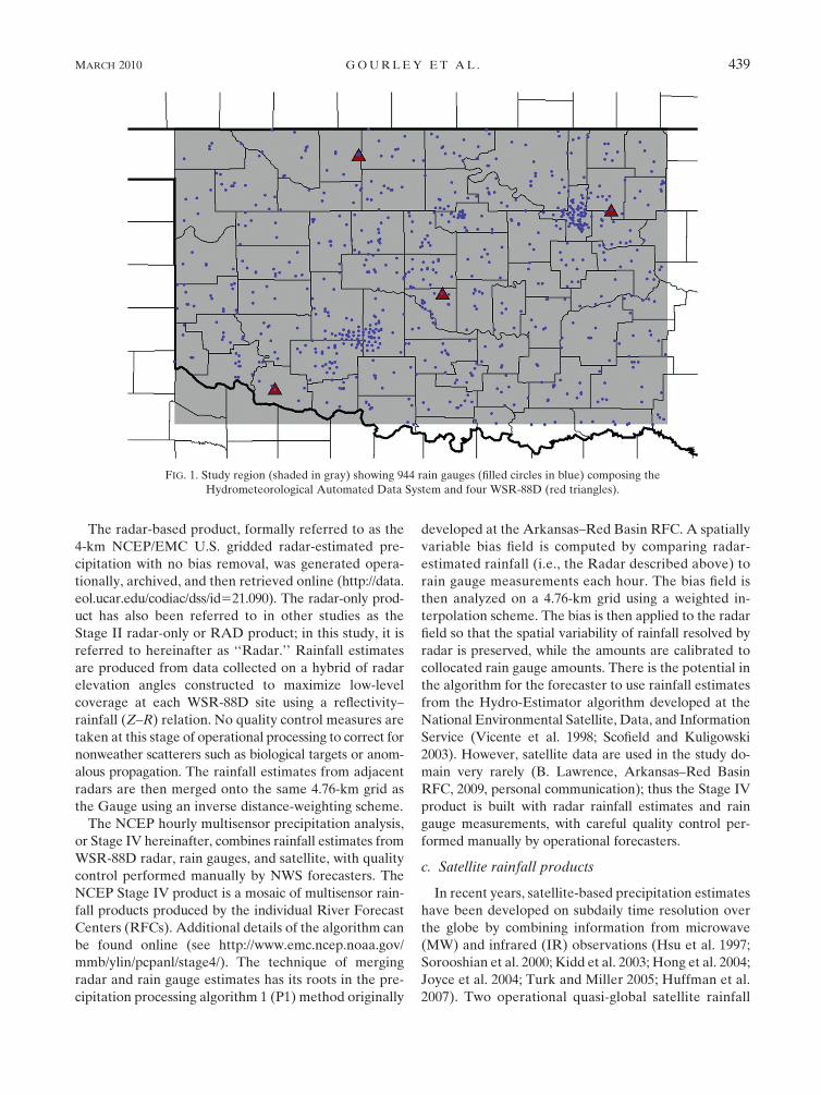
The study domain, extending from 34.08 to 37.08 lati-

tude and from 2100.08 to 295.08 longitude, is shown in

gray in Fig. 1. The blue dots show 944 gauge locations in

the study region composing the Hydrometeorological

Automated Data System (HADS) network operated by

the Office of Hydrologic Development of the U.S. Na-

tional Weather Service (NWS). The red triangles show

four Weather Surveillance Radar-1988 Doppler (WSR-

88D) that are part of the operational Next Generation

Weather Radar (NEXRAD) network. Data from the

gauges and radars shown in Fig. 1 are used to build the

gauge-based, radar-based, and blended radar–gauge–

human rainfall products described below.

b. Ground rainfall products

The gauge-based product used here is the 4-km U.S.

gridded gage-only hourly precipitation analysis developed

for operational use by the National Centers for Envi-

ronmental Prediction (NCEP) Environmental Model-

ing Center (EMC; available online at http://data.eol.

ucar.edu/codiac/dss/id521.088). The product is derived

from automated rain gauge reports from several net-

works with different reporting intervals, maintenance

requirements, gauge types, wind screening, and quality

control procedures applied. Because the gauges are

automated, most of the instruments are either tipping

bucket or weighing gauges. Erroneous rain gauge data

are removed according to a manually edited, infre-

quently updated ‘‘bad gauge list.’’ Rain gauge mea-

surements are objectively analyzed on a grid having

4.76-km spacing using the optimal estimation technique

described in Seo (1998). The method accounts for the

fractional coverage of rainfall due to sparse gauge net-

works and rainfall fields with high spatial variability. A

benefit is accurate delineation of rain versus no-rain

regions. This study refers to the NCEP Stage II gauge-

based product simply as ‘‘Gauge’’ with hourly accumu-

lations available on a 4.76-km grid at the top of each

hour.

438 J O U R N A L O F A P P L I E D M E T E O R O L O G Y A N D C L I M A T O L O G Y VOLUME 49

The radar-based product, formally referred to as the

4-km NCEP/EMC U.S. gridded radar-estimated pre-

cipitation with no bias removal, was generated opera-

tionally, archived, and then retrieved online (http://data.

eol.ucar.edu/codiac/dss/id521.090). The radar-only prod-

uct has also been referred to in other studies as the

Stage II radar-only or RAD product; in this study, it is

referred to hereinafter as ‘‘Radar.’’ Rainfall estimates

are produced from data collected on a hybrid of radar

elevation angles constructed to maximize low-level

coverage at each WSR-88D site using a reflectivity–

rainfall (Z–R) relation. No quality control measures are

taken at this stage of operational processing to correct for

nonweather scatterers such as biological targets or anom-

alous propagation. The rainfall estimates from adjacent

radars are then merged onto the same 4.76-km grid as

the Gauge using an inverse distance-weighting scheme.

The NCEP hourly multisensor precipitation analysis,

or Stage IV hereinafter, combines rainfall estimates from

WSR-88D radar, rain gauges, and satellite, with quality

control performed manually by NWS forecasters. The

NCEP Stage IV product is a mosaic of multisensor rain-

fall products produced by the individual River Forecast

Centers (RFCs). Additional details of the algorithm can

be found online (see http://www.emc.ncep.noaa.gov/

mmb/ylin/pcpanl/stage4/). The technique of merging

radar and rain gauge estimates has its roots in the pre-

cipitation processing algorithm 1 (P1) method originally

developed at the Arkansas–Red Basin RFC. A spatially

variable bias field is computed by comparing radar-

estimated rainfall (i.e., the Radar described above) to

rain gauge measurements each hour. The bias field is

then analyzed on a 4.76-km grid using a weighted in-

terpolation scheme. The bias is then applied to the radar

field so that the spatial variability of rainfall resolved by

radar is preserved, while the amounts are calibrated to

collocated rain gauge amounts. There is the potential in

the algorithm for the forecaster to use rainfall estimates

from the Hydro-Estimator algorithm developed at the

National Environmental Satellite, Data, and Information

Service (Vicente et al. 1998; Scofield and Kuligowski

2003). However, satellite data are used in the study do-

main very rarely (B. Lawrence, Arkansas–Red Basin

RFC, 2009, personal communication); thus the Stage IV

product is built with radar rainfall estimates and rain

gauge measurements, with careful quality control per-

formed manually by operational forecasters.

c. Satellite rainfall products

In recent years, satellite-based precipitation estimates

have been developed on subdaily time resolution over

the globe by combining information from microwave

(MW) and infrared (IR) observations (Hsu et al. 1997;

Sorooshian et al. 2000; Kidd et al. 2003; Hong et al. 2004;

Joyce et al. 2004; Turk and Miller 2005; Huffman et al.

2007). Two operational quasi-global satellite rainfall

FIG. 1. Study region (shaded in gray) showing 944 rain gauges (filled circles in blue) composing the

Hydrometeorological Automated Data System and four WSR-88D (red triangles).


products used in this study are the Tropical Rainfall

Measuring Mission (TRMM) Multisatellite Precipita-

tion Analysis (TMPA; Huffman et al. 2007) and Precip-

itation Estimation from Remotely Sensed Information

using Artificial Neural Networks-Cloud Classification

System (PERSIANN-CCS; Hong et al. 2004).

TMPA provides precipitation estimates by combin-

ing information from multiple satellites as well as rain

gauges depending on sensor availability. The TRMM

products are available 3-hourly at 0.258 3 0.258 spatial

resolution covering the globe 508S–N latitude. TMPA

provides two standard 3B42-level products for the re-

search community: the near-real-time 3B42RT and post-

real-time 3B42V6. The real-time product, 3B42RT, uses

the TRMM Combined Instrument (TCI; TRMM pre-

cipitation radar and TRMM Microwave Imager) dataset

to calibrate precipitation estimates derived from avail-

able low-Earth-orbiting passive microwave radiometers

and then merges all these estimates at 3-h intervals. Gaps

in these analyses are filled using geosynchronous infrared

data regionally calibrated to the merged microwave

product. The post-real-time product, 3B42V6, adjusts

the monthly accumulations of the 3-hourly fields from

3B42RT based on a monthly gauge analysis, including

the Climate Assessment and Monitoring System

(CAMS) 0.58 3 0.58 monthly gauge analysis and the

Global Precipitation Climatology Center (GPCC) 1.08 3

1.08 monthly gauge product. The monthly ratio of the

satellite-only and satellite–gauge combination is used

to rescale the individual 3-h estimates. Therefore, the

gauge-adjusted final product, 3B42V6, has a nominal

resolution of 3-h time step (0000, 0300, . . . , 2100 UTC)

and 0.258 3 0.258 spatial resolution, within the global

latitude belt 508S–508N. More recently, Huffman et al.

(2009) describe how the 3B42RT product is scaled using

the TRMM Combined Instrument. Applying a bias

correction without the need for monthly gauge accu-

mulations will have significant benefits for real-time

users of rainfall products, especially in ungauged basins.

PERSIANN-CCS has been evaluated in the conti-

nental United States for its general performance (Hong

et al. 2004) and in the complex terrain region in western

Mexico for its ability to capture the climatological struc-

ture of precipitation with respect to the diurnal cy-

cle and regional terrain features (Hong et al. 2007). The

PERSIANN-CCS algorithm extracts local and regional

cloud features from infrared geostationary satellite im-

agery in estimating a finer-scale (i.e., 0.048 3 0.048,

30 min) rainfall distribution. PERSIANN-CCS is able

to generate various rain rates at a given brightness

temperature (Tb) and variable rain/no-rain IR thresholds

for different cloud types, which overcomes the one-to-

one mapping limitation of a single Tb–rainfall rate (R)

function for the full spectrum of cloud–rainfall condi-

tions. There are also two versions of PERSIANN-CCS

products available, a real-time (PERSIANN-CCS-RT)

version and a microwave-adjusted (PERSIANN-CCS-

MW) version. First, the PERSIANN-CCS-RT algorithm

processes real-time Geostationary Operational Envi-

ronmental Satellite (GOES) cloud images into pixel rain

rates as described in Hong et al. (2004). Afterward,

in the PERSIANN-CCS-MW algorithm, an automated

neural network for cloud patch–based rainfall estimation,

entitled the Self-Organizing Nonlinear Output (SONO)

model (Hong et al. 2005), was developed to adjust the

real-time product by using composite microwave pre-

cipitation estimates from low-Earth-orbiting satellite

platforms, such as TRMM. The MW-based precipitation

estimates are used to rescale the PERSIANN-CCS-RT

rainfall products on a seasonal (3-monthly) basis. The

real-time data from the current version of PERSIANN-

CCS-RT are available online both at regional (http://

hydis8.eng.uci.edu/CCS/) and global scales (http://hydis8.

eng.uci.edu/GCCS/). However, the PERSIANN-CCS-

MW product is processed and archived after several

days of delay.

The radar, gauge, and Stage IV rainfall products were

produced on an NWS Hydrologic Rainfall Analysis

Project (HRAP) grid having 4.76-km resolution and a

polar stereographic projection. Geographic informa-

tion systems scripts were used to reproject and resample

all NCEP rainfall products onto an analysis grid with

a geographic, or latitude/longitude, projection having

0.048 3 0.048 resolution. The TRMM and PERSIANN-

CCS satellite QPE products were also resampled onto

the same 0.048-resolution grid in geographic coordinates

containing the radar, gauge, and Stage IV products. Be-

cause the native spatial resolution of the TRMM-3B42RT

and TRMM-3B42V6 products is 0.258, the analysis grid

oversamples their values. No interpolation methods

were used in the centroid-based resampling; values co-

incident with the centroid of each analysis grid point

were used directly.

3. Results

a. Seasonal accumulations

Rainfall rates from all products have been accumu-

lated from June to August 2007 to yield seasonal totals

in Fig. 2. The TRMM-3B42RT and TRMM-3B42V6

products are noticeably coarser in resolution compared

to the other products. The TRMM-3B42RT product

identifies rainfall maxima in the central part of the domain.

It also indicates a secondary rainfall maximum in the far

southeast part. The TRMM-3B42V6 product has sub-

stantially lower accumulations than the TRMM-3B42RT


product (Fig. 2b). It is also noted that the spatial pattern

of the seasonal rainfall is different in comparing the

two products. Rainfall in the northwestern part of the

state has been reduced by as much as 500 mm in Fig. 2b,

while the maxima in the eastern and southeastern part of

the state were reduced by approximately 250 mm. The

PERSIANN-CCS-RT and PERSIANN-CCS-MW prod-

ucts have precipitation maxima in the central and north-

ern parts and minima in the far west. The rainfall patterns

in Figs. 2c and 2d resemble each other and those shown

FIG. 2. Accumulated rainfall from June to August

2007 for (a) TRMM-3B42RT, (b) TRMM-3B42V6,

(c) PERSIANN-CCS-RT, (d) PERSIANN-CCS-MW,

(e) Radar, (f) Gauge, and (g) Stage IV. Refer to section 2

for a complete description of each rainfall algorithm.


in Fig. 2a. In comparing the two PERSIANN-CCS prod-

ucts, the rainfall amounts in Fig. 2d are lower by approx-

imately 20% because of the adjustment using passive

microwave rain rates. The Radar has the highest accu-

mulations of all products while rainfall maxima are fo-

cused in a band extending from southwest to northeast,

and a separate region in the southeast (Fig. 2e). Distinct

minima are coincident with three of the radar sites. In

the northwest, there is an apparent blockage to the

southwest of the radar that creates a wedge of anoma-

lously low accumulations. The Gauge in Fig. 2f has the

lowest accumulations of all products and indicates a

band of precipitation extending from the southwest to

northeast and a separate region in the southeast, similar

in shape to the Radar. The Gauge seasonal accumulation

has a smooth appearance, similar to that in Fig. 2b, and

reveals individual rainfall maxima having circular shapes

that are most likely a result of the analysis scheme.

The Stage IV product in Fig. 2g does an admirable job

of mitigating the artifacts noted in Figs. 2e and 2f, cap-

tures the spatial details captured by Radar, and effec-

tively calibrates the Radar amounts to closer agreement

with Gauge accumulations. The Stage IV product has

also had manual quality control procedures applied as

described in section 2. For these reasons, the Stage IV

product will be used as a benchmark, or ground truth,

in comparing the algorithms in forthcoming analyses.

In comparing the TRMM and PERSIANN-CCS rainfall

patterns with Stage IV, Figs. 2a, 2c, and 2d all yield er-

roneously high accumulations in the northwestern part

of the domain. While the Radar, Gauge, and Stage IV

analyses all imply a southwest–northeast orientation of

the heaviest rainfall, the satellite products appear to sug-

gest a more west–east orientation. All satellite products

manage to capture the separate rainfall maximum in the

southeast part of the State, however it is depicted too far

to the south.

To quantify the spatial scales of rainfall resolved by

each of the seasonal accumulations, we have trans-

formed the data shown in Fig. 2 into the frequency do-

main using a discrete Fourier transform. Figure 3 shows

the normalized power spectrum for each QPE algo-

rithm. This analysis indicates that rainfall structures are

poorly resolved by TRMM-3B42RT and TRMM-3B42V6

in comparison with the other products for wavelengths

between 9 and 13 km. The lower bound of 9 km corre-

sponds to the minimum wavelength needed to resolve

the spatial scale of the true seasonal rainfall accumula-

tion. This means a grid with a resolution of twice this

wavelength, or 18 km, would have been sufficient to

capture the inherent spatial rainfall variability. The

TRMM-3B42RT and TRMM-3B42V6 products capture

the spatial rainfall variability for wavelengths greater

than 13 km; this wavelength corresponds to approxi-

mately one-half the resolution of the 0.258 3 0.258 grid

spacing of the TRMM rainfall products.

A quantitative analysis of the rainfall products is pro-

vided by comparing the seasonal accumulations to the

Stage IV product on a cell-by-cell basis, yielding a sam-

ple size of 123 columns by 74 rows in the analysis grid

equaling 9102 points. The validity of the evaluation is

conditional on the accuracy of the Stage IV product, and

thus the reader is encouraged to view these analyses as

relative and not necessarily absolute. The reader is also

reminded that the Stage IV product is not independent

from the Radar or Gauge; we expect to see similarities

between these products because they use the same in-

formation. Scatterplots of Stage IV versus each of the

evaluated QPE algorithms are shown on a log-log scale

in Fig. 4. Each panel indicates the normalized bias (NB

FIG. 3. Normalized power spectrum computed using a discrete Fourier transform for seasonal

accumulations shown in Fig. 2.


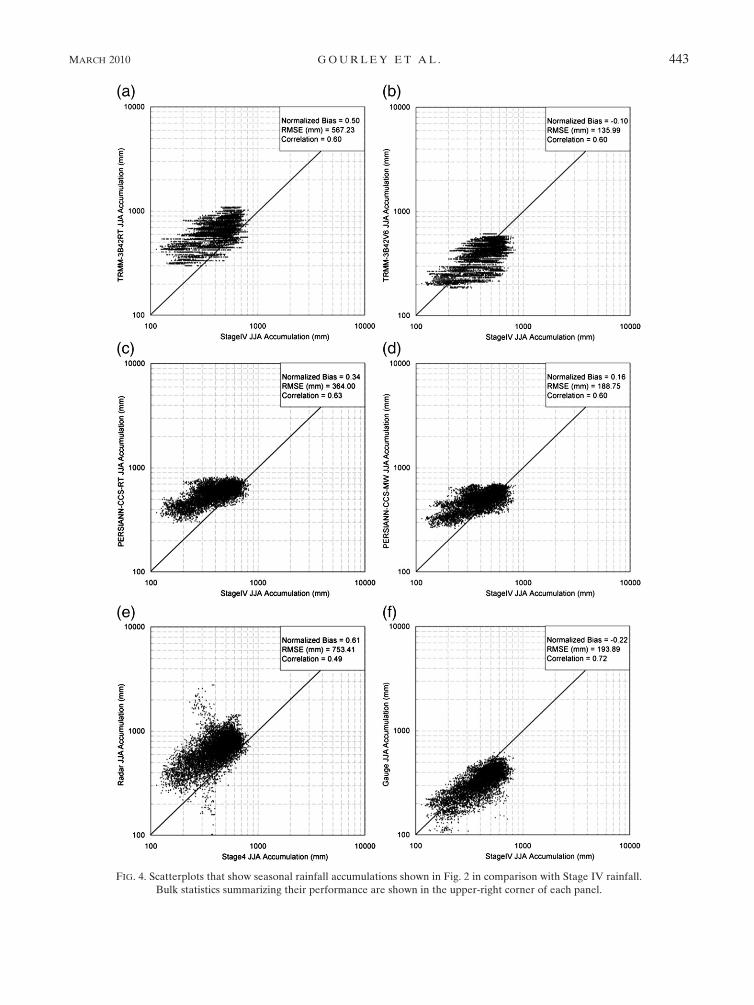
FIG. 4. Scatterplots that show seasonal rainfall accumulations shown in Fig. 2 in comparison with Stage IV rainfall.

Bulk statistics summarizing their performance are shown in the upper-right corner of each panel.


hereinafter), root-mean-square error computed after the

bias was removed (RMSE hereinafter), and Pearson cor-

relation coefficient (CORR), defined as follows:

NB 5�QPE

i� StageIV

i

�StageIVi

, (1)

RMSE 5 QPE 3�StageIV

i

�QPEi

� StageIV

0@

1A

2* +1/2

, (2)

and

CORR 5cov(QPE, StageIV)

sQPE

sStageIV

, (3)

where NB is dimensionless, RMSE is in millimeters, and

CORR is dimensionless. The angled brackets in (2) refer

to averaging. In the computation of CORR, cov refers to

the covariance, and s is the standard deviation. NB,

when multiplied by 100, gives the degree of overesti-

mation or underestimation in percentage.

The real-time TRMM product, TRMM-3B42RT, over-

estimated rainfall by 50%, had an RMSE of 567 mm

and a comparatively good CORR of 0.60 (Fig. 4a). The

TRMM-3B42V6 product had the lowest NB of 20.10,

indicating underestimation of 10% (Fig. 4b). This product

also had the lowest RMSE (136 mm) when compared with

the other algorithms. The PERSIANN-CCS-RT product

performed better than TRMM-3B42RT according to all

three statistics (Fig. 4c). The PERSIANN-CCS-MW prod-

uct offered improvements over PERSIANN-CCS-RT in

terms of cutting the NB and RMSE approximately in half

but reduced the CORR from 0.63 to 0.60 (Fig. 4d). Over-

estimation with the Radar algorithm was 61%; this algo-

rithm also had the largest scatter as represented with an

RMSE of 753 mm and lowest CORR of 0.49 (Fig. 4e). The

Gauge, on the other hand, underestimated rainfall by 22%

(Fig. 4f). The Gauge had the highest CORR of all QPE

algorithms at 0.72. In summary, the best overall perfor-

mance in terms of seasonal NB and RMSE was with the

TRMM-3B42V6 product despite its coarse resolution,

while the worst overall performance was with Radar. It is

noteworthy that both satellite algorithms that had no

gauge adjustment (i.e., TRMM-3B42RT and PERSIANN-

CCS-RT) outperformed the unadjusted Radar in terms of

all three performance measures. At the seasonal time

scale, it appears that satellite is superior to radar prior to

the application of rain gauge adjustments.

b. Daily statistics

Daily accumulations were created for the PERSIANN-

CCS-RT, PERSIANN-CCS-MW, Radar, Gauge, and

Stage IV products by simply adding up 24 hourly accu-

mulations for each day. The TRMM rainfall products

are available on a nominal 3-hourly basis at 0000, 0300,

0600, 0900, 1200, 1500, 1800, and 2100 UTC as described

in Huffman et al. (2007). The accumulations were cen-

tered on the nominal observation times at which the

passive microwave fields were converted to precipita-

tion estimates. Daily accumulations were created by

summing the files from 0300 to 2100 UTC plus one-half

the 0000 UTC accumulation of the same day and one-

half the 0000 UTC accumulation for the next day. Once

again, we assume the Stage IV product is the benchmark

and compare daily accumulations from each of the al-

gorithms on a cell-by-cell basis. The sample size is 123 3

74 3 92 5 837 384 corresponding to the number of col-

umns and rows composing the analysis grid and number

of days in June–August.

The same bulk statistics used in the seasonal evalua-

tion in section 3a are used here, but were computed on

a daily basis and are thus shown as histograms of NB,

RMSE, and CORR (Fig. 5). Figure 5a indicates Radar

had the largest, or worst, NB with a mode in the 60%

overestimation bin, while the Gauge product had the

best NB with a mode in the 0% bin. The TRMM-

3B42V6 reanalysis product improved over its real-time

counterpart by shifting the distribution closer to the

0% bin. The distributions for PERSIANN-CCS-RT and

PERSIANN-CCS-MW are similar with the latter prod-

uct offering some improvement at the tails of the dis-

tribution and increasing the frequency of points falling

in the 0% bin. The histograms of daily RMSE values

in Fig. 5b show that Radar had the highest RMSE, sim-

ilar to the seasonal analysis shown in the previous sec-

tion. The Gauge, TRMM-3B42RT, and TRMM-3B42V6

products had lower RMSE values than either of the

PERSIANN-CCS products. The PERSIANN-CCS-MW

product offered no clear improvement in terms of daily

RMSE over the PERSIANN-CCS-RT product. The

TRMM-3B42V6 product, on the other hand, yielded

a lower RMSE than TRMM-3B42RT. Histograms of

daily CORR in Fig. 5c show Gauge and then Radar had

the best performance with modal values at 0.8. The next

best CORR was associated with the TRMM-3B42V6

product. The real-time TRMM product performed bet-

ter than both the PERSIANN-CCS products, with the

PERSIANN-CCS-RT product yielding slightly higher

CORR values than PERSIANN-CCS-MW.

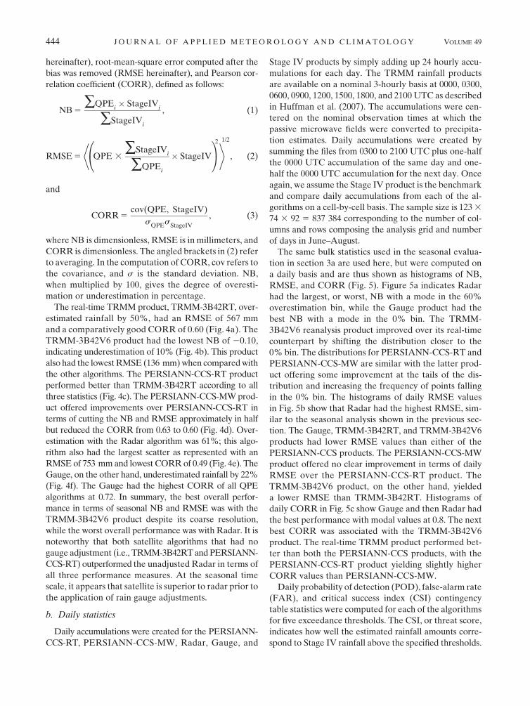
Daily probability of detection (POD), false-alarm rate

(FAR), and critical success index (CSI) contingency

table statistics were computed for each of the algorithms

for five exceedance thresholds. The CSI, or threat score,

indicates how well the estimated rainfall amounts corre-

spond to Stage IV rainfall above the specified thresholds.


Perfect skill occurs with a CSI value of 1. The thresholds

of 0.3, 1.3, 5.3, 17.4, and 51.1 mm were chosen based on

the 5%, 25%, 50%, 75%, and 95% exceedance quantiles

of the Stage IV daily accumulation histogram (not shown).

The reader is reminded that these thresholds apply

specifically to a season of record rainfall in Oklahoma

and are not directly transferrable to other regions. The

Gauge had the highest POD when considering 95% of

the data distribution (Fig. 6a). However, Radar had the

highest POD with the upper 50%, 25%, and 5% of the

daily rainfall distribution. In fact, at the upper end,

Gauge had the lowest detection capabilities. This is an

expected result because rainfall maxima are rarely co-

incident with gauge locations but are captured by radar.

TRMM-3B42RT had equivalent or better POD than

PERSIANN-CCS-RT at all thresholds. The TRMM-

3B42V6 and PERSIANN-CCS-MW performed simi-

larly to each other and detected rainfall events better

than their real-time counterparts at the lowest threshold,

but less so for the upper 50%, 25%, and 5% thresholds.

All algorithms tended toward lower POD values with

increasing rainfall intensity.

The FAR was lowest with Gauge for all rainfall

thresholds. The next lowest FAR was associated with

TRMM-3B42V6. Radar had the highest FAR at the

lowest threshold and then converged toward FAR values

of the other satellite-based algorithms at the higher rain-

fall thresholds. FAR with PERSIANN-CCS-MW was

higher than PERSIANN-CCS-RT for the upper 95%

and 75% of the data distribution, indicating degradation

in performance when microwave data were included.

With the exception of Gauge, all algorithms tended to-

ward higher FAR within increasing rainfall intensity.

The CSI, or algorithm skill, indicates the best per-

formance was with Gauge for the upper 95%, 75%,

50%, and 25% of the Stage IV daily rainfall distribution

(Fig. 6c). Interestingly, Radar was the worst performer

considering 95% of the rainfall distribution, but best

with high-intensity rainfall. TRMM-3B42V6 was better

than or at least equivalent to TRMM-3B42RT and the two

PERSIANN-CCS products for all thresholds. As noted

in the daily analysis of bulk statistics, the PERSIANN-

CCS-RT product outperformed PERSIANN-CCS-MW

for daily rainfall accumulations. All algorithms had re-

duced skill with increasing rainfall intensity.

c. Hourly composites

Hourly rainfall composites were created by comput-

ing grids of average rainfall rate for each hour in the

3-month dataset. Figure 7a shows a time series plot of

the average hourly rainfall rates, considering all grid

cells in the domain (Fig. 1), for the Stage IV rainfall

product. We conducted this analysis both with and without

FIG. 5. Histograms of (a) NB, (b) RMSE with bias removed, and

(c) Pearson correlation coefficient for daily rainfall accumulations

from June to August 2007 estimated from each algorithm denoted

in legend. Stage IV was considered as reference, or ground truth.


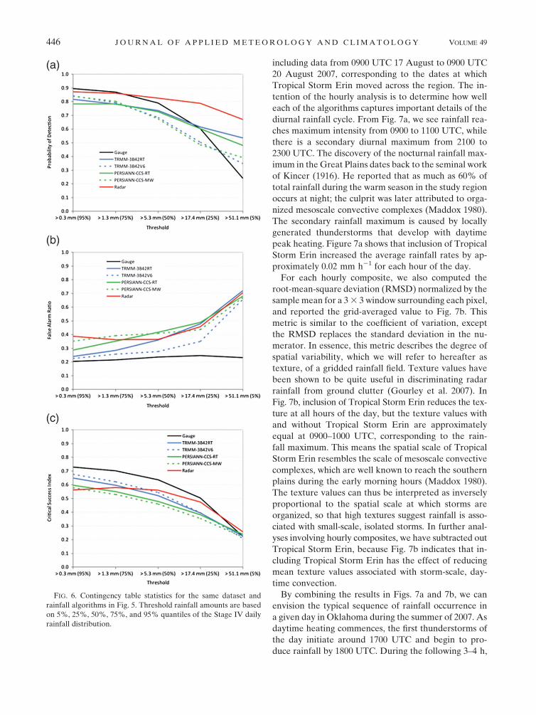
including data from 0900 UTC 17 August to 0900 UTC

20 August 2007, corresponding to the dates at which

Tropical Storm Erin moved across the region. The in-

tention of the hourly analysis is to determine how well

each of the algorithms captures important details of the

diurnal rainfall cycle. From Fig. 7a, we see rainfall rea-

ches maximum intensity from 0900 to 1100 UTC, while

there is a secondary diurnal maximum from 2100 to

2300 UTC. The discovery of the nocturnal rainfall max-

imum in the Great Plains dates back to the seminal work

of Kincer (1916). He reported that as much as 60% of

total rainfall during the warm season in the study region

occurs at night; the culprit was later attributed to orga-

nized mesoscale convective complexes (Maddox 1980).

The secondary rainfall maximum is caused by locally

generated thunderstorms that develop with daytime

peak heating. Figure 7a shows that inclusion of Tropical

Storm Erin increased the average rainfall rates by ap-

proximately 0.02 mm h21 for each hour of the day.

For each hourly composite, we also computed the

root-mean-square deviation (RMSD) normalized by the

sample mean for a 3 3 3 window surrounding each pixel,

and reported the grid-averaged value to Fig. 7b. This

metric is similar to the coefficient of variation, except

the RMSD replaces the standard deviation in the nu-

merator. In essence, this metric describes the degree of

spatial variability, which we will refer to hereafter as

texture, of a gridded rainfall field. Texture values have

been shown to be quite useful in discriminating radar

rainfall from ground clutter (Gourley et al. 2007). In

Fig. 7b, inclusion of Tropical Storm Erin reduces the tex-

ture at all hours of the day, but the texture values with

and without Tropical Storm Erin are approximately

equal at 0900–1000 UTC, corresponding to the rain-

fall maximum. This means the spatial scale of Tropical

Storm Erin resembles the scale of mesoscale convective

complexes, which are well known to reach the southern

plains during the early morning hours (Maddox 1980).

The texture values can thus be interpreted as inversely

proportional to the spatial scale at which storms are

organized, so that high textures suggest rainfall is asso-

ciated with small-scale, isolated storms. In further anal-

yses involving hourly composites, we have subtracted out

Tropical Storm Erin, because Fig. 7b indicates that in-

cluding Tropical Storm Erin has the effect of reducing

mean texture values associated with storm-scale, day-

time convection.

By combining the results in Figs. 7a and 7b, we can

envision the typical sequence of rainfall occurrence in

a given day in Oklahoma during the summer of 2007. As

daytime heating commences, the first thunderstorms of

the day initiate around 1700 UTC and begin to pro-

duce rainfall by 1800 UTC. During the following 3–4 h,

FIG. 6. Contingency table statistics for the same dataset and

rainfall algorithms in Fig. 5. Threshold rainfall amounts are based

on 5%, 25%, 50%, 75%, and 95% quantiles of the Stage IV daily

rainfall distribution.


convectively driven storms become more numerous and

remain isolated as noted with texture values of 0.55. A

relative maximum in rainfall rates of 0.19 mm h21 is

reached from 2100 to 2200 UTC. At 2200 UTC, the

thunderstorms begin to decay in association with loss

of daytime heating. A secondary rainfall minimum of

0.12 mm h21 is reached at 0400 UTC. Then, a gradual

increase in grid-averaged rainfall rates occurs through-

out the night reaching an overall maximum value of

0.26 mm h21 from 0900 to 1100 UTC. The texture

values with this nocturnal rainfall maximum are 0.3, or

approximately half the values associated with the di-

urnal rainfall maximum. The mesoscale convective com-

plexes impacting the region during the early morning

hours are organized on a larger scale and propagate

across the region as opposed to initiating within the

study domain, which is the case with the diurnal rainfall

maximum organized at the storm scale. Rainfall rates

continue to decrease after 1100 UTC and textures in-

crease until the minimum rainfall rate of 0.11 mm h21 is

reached at 1700 UTC. Hourly rainfall composites and

their textures are examined for each rainfall algorithm

to determine how well they describe the typical hourly

sequence of rainfall occurrence during an average day in

the summer of 2007.

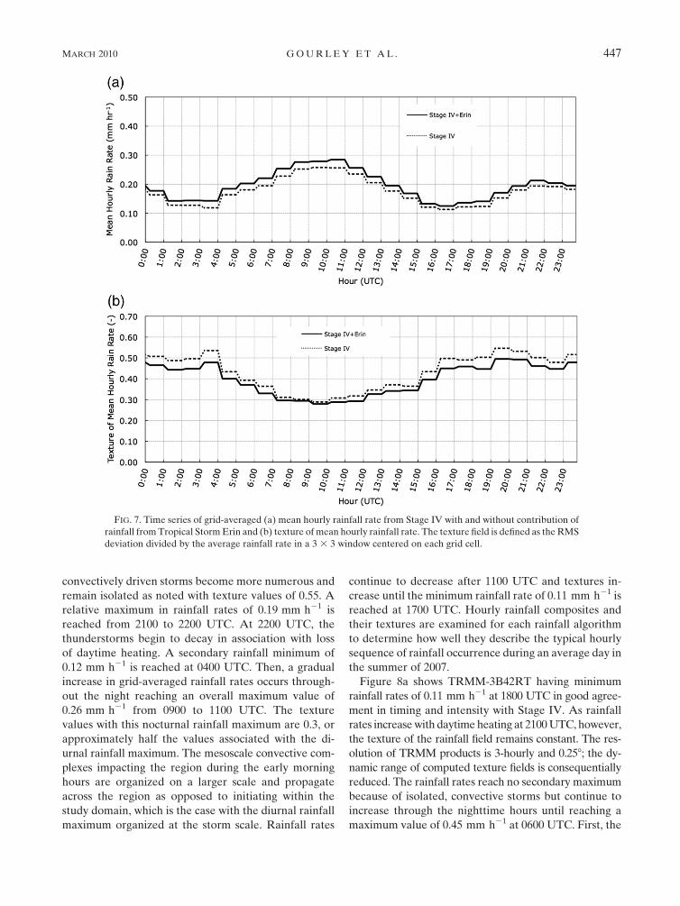
Figure 8a shows TRMM-3B42RT having minimum

rainfall rates of 0.11 mm h21 at 1800 UTC in good agree-

ment in timing and intensity with Stage IV. As rainfall

rates increase with daytime heating at 2100 UTC, however,

the texture of the rainfall field remains constant. The res-

olution of TRMM products is 3-hourly and 0.258; the dy-

namic range of computed texture fields is consequentially

reduced. The rainfall rates reach no secondary maximum

because of isolated, convective storms but continue to

increase through the nighttime hours until reaching a

maximum value of 0.45 mm h21 at 0600 UTC. First, the

FIG. 7. Time series of grid-averaged (a) mean hourly rainfall rate from Stage IV with and without contribution of

rainfall from Tropical Storm Erin and (b) texture of mean hourly rainfall rate. The texture field is defined as the RMS

deviation divided by the average rainfall rate in a 3 3 3 window centered on each grid cell.


intensity of this maximum value is .70% too high. Even

with the coarse, 3-hourly temporal resolution, the noc-

turnal rainfall maximum is reached too early. Mesoscale

convective complexes are well known to be associated

with large cirrus cloud shields. It is quite plausible that

the cirrus cloud contamination results in the satellite-

based timing error associated with the nocturnal rainfall

maximum. TRMM products at 0900 or 1200 UTC are

closer to the rainfall maximum as depicted by Stage IV.

The TRMM-3B42RT product does, however, correctly

portray a texture minimum at 0900 UTC.

The TRMM-3B42V6 product yields a very similar

sequence of rainfall rates as TRMM-3B42RT, but with

lower mean values reaching 0.26 mm h21 at 0600 UTC.

The timing of the nocturnal maximum is approximately

4 h too early, but the intensity agrees almost perfectly

with Stage IV. The texture values from TRMM-3B42V6

are very similar to those of TRMM-3B42RT, but slightly

lower and thus more erroneous for the daytime con-

vection at 1800 and 2100 UTC. In general, the TRMM

rainfall products depict the nocturnal rainfall maximum

too early, do not indicate the secondary, diurnal maxi-

mum in rainfall rates, and do little to distinguish between

the scale differences in the precipitation that produces

the nocturnal and diurnal maxima. The intensity of the

TRMM-3B42RT rainfall minimum, however, matches

that of Stage IV, and the maximum rainfall rate of

0.26 mm h21 from TRMM-3B42V6 is very close to the

Stage IV maximum.

The PERSIANN-CCS-RT product in Fig. 8a has

minimum rainfall rates at 1700 UTC in very good agree-

ment with the timing of Stage IV. As daytime heating

commences, rainfall rates increase to 0.29 mm h21 at

2200 UTC, which overestimates the intensity of the

Stage IV diurnal maximum, but the timing of the diurnal

maximum is excellent. Then, rainfall rates decrease until

FIG. 8. As in Fig. 7, but for all rainfall algorithms examined in this study. The rainfall from Tropical Storm Erin has

been omitted.


0200 UTC when the gradual increase with the nocturnal

rainfall maximum begins. In comparison with Stage IV,

the onset of this increase is approximately 2 h too early.

The nocturnal maximum in rainfall rates is reached at

0700 UTC with values of 0.43 mm h21. Similar to the

TRMM-3B42RT rainfall product, the timing of the

maximum is approximately 3 h too early and the inten-

sity is 65% too high. The cirrus cloud shields associated

with mesocale convective systems are the likely culprit

for this error affecting TRMM and PERSIANN-CCS

rainfall products. The texture field with PERSICANN-

CCS-RT reaches a maximum value of 0.51 at 1900 UTC

in good agreement with Stage IV. Texture values de-

crease much more rapidly than Stage IV following the

diurnal rainfall maximum and hit a minimum of 0.12

at 0700 UTC. This minimum texture value is too low

and is reached about 3 h too early. Nonetheless, the

PERSIANN-CCS-RT product does distinguish between

the diurnal and nocturnal spatial scales of rainfall.

The PERSIANN-CCS-MW product shows the same

trend in rainfall rates, but the values are approximately

0.03 mm h21 lower in intensity. The lower intensities are

in better agreement with Stage IV from 1900 to 0800 UTC,

or just a little over half the time. In terms of depicting

spatial scales of rainfall, the PERSIANN-CCS-MW prod-

uct lowers the texture values at all times, which is incorrect

according to Stage IV texture values. This lowering of the

texture is likely due to the coarseness of the MW data (10–

30 km), which was used to rescale the PERSIANN-CCS-

RT product to yield PERSIANN-CCS-MW. In addition,

the most correct aspect of the PERSIANN-CCS-RT tex-

ture time series, that is, the maximum of 0.51 at 1900 UTC,

has been dramatically reduced to 0.29 and is now too

early with its timing following inclusion of the micro-

wave data. In summary, the PERSIANN-CCS products

have similar errors as the TRMM rainfall products in

that they depict the nocturnal rainfall maximum too

early. They improve over TRMM in correctly resolving

the secondary diurnal rainfall maximum probably due to

higher temporal resolution. Moreover, the PERSIANN-

CCS-RT product shows the capability of being able to

differentiate the scales of precipitation that result in

the nocturnal and diurnal rainfall maxima. Similar to

results found with the daily statistics in section 3b, the

PERSIANN-CCS-MW product offers no improvements

over PERSIANN-CCS-RT.

Radar and Gauge, which the reader is reminded are

both inputs to Stage IV, have very similar trends as Stage

IV in Fig. 8a. There is a slight difference in the timing

of the nocturnal maximum with Radar reaching values

of 0.43 mm h21 at 0900 UTC, 1 h prior to the Stage IV

and Gauge maximum. In general, it appears as though

Stage IV has been adjusted to agree more closely with

the Gauge rainfall values and timing, which helps to

explain the aforementioned timing difference. The time

series of texture values in Fig. 8b, however, reveals Stage

IV appropriately benefits from the ability of Radar to

distinguish between the storm-scale diurnal maximum

and the mesoscale nocturnal maximum. Future multi-

sensor rainfall products can likewise benefit from the

PERSIANN-CCS-RT product’s ability to segregate

the scale differences between the two rainfall maxima.

The Gauge product, on the other hand, has no capability

whatsoever to differentiate between these scales of or-

ganized precipitation.

4. Summary and conclusions

In this study, we have compared rainfall estimates

from algorithms based on measurements from satellite,

radar, rain gauges, and combinations to highlight their

relative performance for seasonal, daily, and hourly time

scales. This multitiered analysis considers the ability to

resolve precipitation characteristics at different spatial

scales and as a function of rainfall intensity. The study

domain is in a heavily instrumented region in terms of

radar coverage and gauge density. The topography in

the study region is relatively flat and the rainfall is pri-

marily from intense, convective storms; thus, the trans-

ferability of the results in this study may not directly

apply to other regimes. Results drawn from the analysis

of seasonal rainfall totals from June to August 2007 in

Oklahoma are summarized as follows:

d Gauge had the highest CORR of 0.72, but under-

estimated rainfall by 22%.d The Stage II radar product had the worst overall per-

formance with overestimation of 61%, highest RMSE

of 753 mm, and lowest CORR. Artifacts due to beam

blockages were noted in the seasonal accumulation

product.d Despite the TRMM-3B42V6 product having rela-

tively coarse 0.258 spatial resolution, it had the best

agreement with the Stage IV product, which was con-

sidered as reference or ground truth, in terms of NB of

20.10 and RMSE of 136 mm.d The PERSIANN-CCS-RT product had better per-

formance than TRMM-3B42RT according to all ana-

lyzed statistics.d The PERSIANN-CCS-MW product offered improve-

ments over PERSIANN-CCS-RT in terms of cutting

the NB and RMSE approximately in half but reduced

the CORR from 0.63 to 0.60.

Rainfall rates were accumulated on a daily basis and

then evaluated using histograms of NB, RMSE, and

CORR bulk statistics as above, considering Stage IV as


a reference. In addition, we computed contingency table

statistics for five rainfall thresholds—0.3, 1.3, 5.3, 17.4,

and 51.1 mm—corresponding to the 95%, 75%, 50%,

25%, and 5% exceedance quantiles of the Stage IV daily

rainfall distribution. Results from the daily rainfall anal-

ysis are summarized as follows:

d Gauge had the best performance according to the CSI

for the upper 95%, 75%, 50%, and 25% of the data

distribution, but worst probability of detection for the

upper 5%, corresponding to extreme rainfall amounts.d Radar, on the other hand, was the worst performer when

considering rainfall accumulations .0.3 mm, but best

when restricting the data sample to rainfall .51.1 mm.d For the 95%, 75%, 50%, and 25% exceedance thresh-

olds, TRMM products had generally higher skill than

PERSIANN-CCS products, with the 3B42V6 being the

best.d Although having a lower CSI than TRMM-3B42V6 at

low–medium rainfall intensity, PERSIANN-CCS-RT

had the second highest skill, after Radar, at the upper

5% rainfall threshold.d All rainfall algorithms had reduced skill with in-

creasing rainfall rate.

The third analysis examined hourly rainfall compos-

ites from each algorithm and plotted their average

rainfall rates and texture fields as a daily composite time

series. The following results are summarized from the

hourly analysis:

d All satellite-based products depicted the nocturnal

rainfall maximum 3–4 h too early, presumably be-

cause of large cirrus shields associated with mesoscale

convective complexes.d The relatively coarse, 3-hourly resolution with the

TRMM-3B42RT and TRMM-3B42V6 products in-

hibited their ability to properly identify the secondary,

diurnal maximum in rainfall rates.d The texture fields indicated that Gauge was unable to

discriminate scale differences between nocturnal and

diurnal rainfall maxima.d PERSIANN-CCS-RT was the only satellite-based al-

gorithm that adequately depicted the high spatial vari-

ability associated with storm-scale rainfall resulting from

daytime heating.

In summary, the Stage IV product was used as a ref-

erence dataset. It was shown to be precise with the in-

corporation of spatial rainfall variability captured by

radar while maintaining accuracy through the use of

rain gauge accumulations. The ability to be simulta-

neously precise and accurate through the intelligent use

of in situ and remote sensing platforms is a desirable

characteristic of multisensor rainfall algorithms. Some

potential pitfalls of the Stage IV product are quality

control issues with hourly rain gauge reports and beam

blockages seen in the radar data. Improvements can be

expected with improved manual and automatic data

quality control methods as well as using climatological

radar rainfall maps to identify beam blockages and sub-

sequently modifying hybrid scan lookup tables.

Physical limitations associated with low-Earth-orbiting

satellites meant the spatiotemporal resolution of TRMM

rainfall products was incapable of properly representing

the diurnal cycle of rainfall in the study domain, in spite

of the fact that IR data are used as input to the TRMM

3B42 algorithms (Huffman et al. 2007). The spectral

analysis also revealed the lack of spatial details offered

by TRMM for wavelengths up to 13 km, corresponding

to approximately one-half the resolution of the 0.258 3

0.258 gridcell spacing. The result was the inability of

TRMM rainfall products to distinguish between the me-

soscale and storm-scale nature of nocturnal and diurnal

convection. This is a major limitation if the TRMM

products are to be considered for small-scale applica-

tions (e.g., flash floods and diurnal rainfall studies) in

ungauged regions. The monthly gauge bias correction to

the TRMM-3B42RT product to yield TRMM-3B42V6

resulted in significant improvements at all temporal

scales. First, this result highlights the significance of

performing bias correction, typically done with rain

gauge accumulations, on remotely sensed rainfall esti-

mates. Although recent work by Huffman et al. (2009)

demonstrates how the TCI, in lieu of rain gauges, can be

used to scale the TRMM-3B42RT product. Second, the

gauge correction was performed on a monthly basis, yet

improvements were realized submonthly at daily and

hourly time scales. This result indicates the TRMM-

3B42RT product has error, but the bias is stationary and

thus readily correctable.

The relatively high spatiotemporal resolution with

the GOES-based PERSIANN-CCS-RT product enabled

it to distinguish rainfall-scale differences on an hourly

basis, which justifies its use in diurnal rainfall studies in

ungauged regions over TRMM rainfall products. It is

noteworthy that the adjustment of PERSIANN-CCS-

RT with MW data from low-Earth-orbiting satellites,

yielding PERSIANN-CCS-MW, resulted in some im-

provements at the seasonal time scale but degraded

performance at daily and hourly scales. Incorporation of

MW data is meant to correct rainfall bias in a similar

manner to rain gauges, but the coarseness of the MW

data (10–30 km) is evidently not as sufficient as gauge

data to remove bias at these smaller time scales. In ad-

dition, the update interval of recalibrating PERSIANN-

CCS-RT with MW is seasonal (3-monthly), which lacks


adequate sensitivity to differences in precipitation re-

gimes, particularly at smaller time scales such as daily or

hourly. Another contributing cause might be the prob-

lematic bias of MW-based rain rates over land. Future

algorithms utilizing PERSIANN-CCS rainfall products

should consider using rain gauge accumulations on a

monthly basis to correct bias in a similar manner to

TRMM-3B42V6. The gauge-based monthly bias cor-

rections are not available in real time; therefore, only

users who are not adversely affected by the time lag (e.g.,

water resources) will benefit. Analyzing PERSIANN-

CCS-RT with gauge bias correction at submonthly time

scales (i.e., daily and/or hourly) will reveal whether the

bias has a transient or stationary character. This kind of

analysis will shed light on the update interval required

for future recalibration strategies.

We envision that readers of this work, as well as rain-

fall algorithm developers, will capitalize on the benefits

provided from each algorithm so they may be used in an

optimal way (i.e., using a multisensor approach) to yield

the most skillful rainfall products. This optimization step

is particularly necessary for rainfall estimation in regions

that may not have the availability of high-density in-

struments. For example, radar data void in the conter-

minous United States have been rigorously quantified

in Maddox et al. (2002), while various gauge network

maps show data densities and are widely available on

the Internet. Future work coming from this study will

be the development of a multisensor rainfall algorithm

that utilizes information from radar, satellite, and gauges,

and optimizes their contribution to the final product based

on spatial scale, temporal scale, and rainfall intensity.

Another topic inviting future research is evaluating the

various rainfall algorithms as inputs to a calibrated hy-

drologic model at multiple temporal and spatial scales

and discharge quantiles, including flash-flooding events.

Acknowledgments. Funding was provided by NOAA/

Office of Oceanic and Atmospheric Research under

NOAA/University of Oklahoma Cooperative Agree-

ment NA17RJ1227, U.S. Department of Commerce.

Stage II radar- and gauge-based products were provided

by NCAR/EOL under sponsorship of the National Sci-

ence Foundation (http://data.eol.ucar.edu/). The Stage

IV rainfall product was obtained at the National Weather

Service’s National Precipitation Verification Unit (http://

www.hpc.ncep.noaa.gov/npvu/). The authors gratefully

acknowledge Dr. Soroosh Sorooshian at the University of

California, Irvine, and Dr. George Huffman at NASA

Goddard for providing the PERSIANN-CCS and TMPA

products in this study, respectively. Reviews from

Dr. George Huffman and two anonymous reviewers

improved the quality of this manuscript.

REFERENCES

Anagnostou, E. N., 2004: Overview of overland satellite rainfall

estimation for hydro-meteorological applications. Surv. Geo-

phys., 25, 511–537.

Arndt, D. S., J. B. Basara, R. A. McPherson, B. G. Illston,

G. D. McManus, and D. B. Demko, 2009: Observations of the

overland reintensification of Tropical Storm Erin (2007). Bull.

Amer. Meteor. Soc., 90, 1079–1093.

Austin, P. M., 1987: Relation between measured radar reflectivity

and surface rainfall. Mon. Wea. Rev., 115, 1053–1070.

Ciach, G. J., 2003: Local random errors in tipping-bucket rain gauge

measurements. J. Atmos. Oceanic Technol., 20, 752–759.

Ebert, E. E., J. E. Janowiak, and C. Kidd, 2007: Comparison

of near-real-time precipitation estimates from satellite ob-

servations and numerical models. Bull. Amer. Meteor. Soc.,

88, 47–64.

Gebremichael, M., and W. F. Krajewski, 2004: Characterization

of the temporal sampling error in space-time-averaged rain-

fall estimates from satellites. J. Geophys. Res., 109, D11110,

doi:10.1029/2004JD004509.

Gourley, J. J., R. A. Maddox, D. W. Burgess, and K. W. Howard,

2002: An exploratory multisensor technique for quantitative

estimation of stratiform rainfall. J. Hydrometeor., 3, 166–180.

——, P. Tabary, and J. Parent-du-Chatelet, 2007: A fuzzy logic

algorithm for the separation of precipitating from non-

precipitating echoes using polarimetric radar observations.

J. Atmos. Oceanic Technol., 24, 1439–1451.

Hong, Y., K.-L. Hsu, S. Sorooshian, and X. Gao, 2004: Pre-

cipitation estimation from remotely sensed imagery using an

artificial neural network cloud classification system. J. Appl.

Meteor., 43, 1834–1853.

——, ——, ——, and ——, 2005: Self-organizing nonlinear output

(SONO): A neural network suitable for cloud patch–based

rainfall estimation at small scales. Water Resour. Res., 41,

W03008, doi:10.1029/2004WR003142.

——, ——, H. Moradkhani, and S. Sorooshian, 2006: Uncertainty

quantification of satellite rainfall estimation and Monte Carlo

assessment of the error propagation into hydrologic response.

Water Resour. Res., 42, W08421, doi:10.1029/2005WR004398.

——, D. Gochis, J. T. Chen, K.-L. Hsu, and S. Sorooshian, 2007:

Evaluation of Precipitation Estimation from Remote Sensed

Information using Artificial Neural Network-Cloud Classi-

fication System (PERSIANN-CCS) rainfall measurement

using the NAME event rain gauge network. J. Hydrometeor.,

8, 469–482.

Hossain, F., and G. J. Huffman, 2008: Investigating error metrics

for satellite rainfall data at hydrologically relevant scales.

J. Hydrometeor., 9, 563–575.

Hsu, K.-L., X. Gao, S. Sorooshian, and H. V. Gupta, 1997: Pre-

cipitation estimation from remotely sensed information using

artificial neural networks. J. Appl. Meteor., 36, 1176–1190.

Huffman, G. J., and Coauthors, 2007: The TRMM multisatellite

precipitation analysis (TMPA): Quasi-global, multiyear,

combined-sensor precipitation estimates at fine scale. J. Hy-

drometeor., 8, 38–55.

——, R. F. Adler, D. T. Bolvin, and E. J. Nelkin, 2009: The TRMM

Multisatellite Precipitation Analysis (TMPA). Satellite Rain-

fall Applications for Surface Hydrology, F. Hossain and

M. Gebremichael, Eds., Springer Verlag, 3–22.

Joss, J., and A. Waldvogel, 1990: Precipitation measurements and

hydrology. Radar in Meteorology, D. Atlas, Ed., Amer. Me-

teor. Soc., 577–606.


Joyce, R. J., J. E. Janowiak, P. A. Arkin, and P. Xie, 2004:

CMORPH: A method that produces global precipitation es-

timates from passive microwave and infrared data at high

spatial and temporal resolution. J. Hydrometeor., 5, 487–503.

Kidd, C., D. R. Kniveton, M. C. Todd, and T. J. Bellerby, 2003:

Satellite rainfall estimation using combined passive micro-

wave and infrared algorithms. J. Hydrometeor., 4, 1088–1104.

Kincer, J. B., 1916: Daytime and nighttime precipitation and their

economic significance. Mon. Wea. Rev., 44, 628–633.

Legates, D. R., and T. L. DeLiberty, 1993: Precipitation mea-

surement biases in the United States. Water Resour. Bull., 29,

855–861.

Maddox, R. A., 1980: Mesoscale convective complexes. Bull. Amer.

Meteor. Soc., 61, 1374–1387.

——, J. Zhang, J. J. Gourley, and K. W. Howard, 2002: Weather

radar coverage over the contiguous United States. Wea. Fore-

casting, 17, 927–934.

Marselek, J., 1981: Calibration of the tipping-bucket raingage.

J. Hydrol., 53, 343–354.

Nystuen, J. A., 1999: Relative performance of automatic rain

gauges under different rainfall conditions. J. Atmos. Oceanic

Technol., 16, 1025–1043.

Scofield, R. A., and R. J. Kuligowski, 2003: Status and outlook

of operational satellite precipitation algorithms for extreme-

precipitation events. Wea. Forecasting, 18, 1037–1051.

Seo, D.-J., 1998: Real-time estimation of rainfall fields using radar

rainfall and rain gage data. J. Hydrol., 208, 37–52.

Sorooshian, S., K.-L. Hsu, X. Gao, H. V. Gupta, B. Imam, and

D. Braithwaite, 2000: An evaluation of PERSIANN system

satellite-based estimates of tropical rainfall. Bull. Amer. Me-

teor. Soc., 81, 2035–2046.

Steiner, M., T. L. Bell, Y. Zhang, and E. F. Wood, 2003: Com-

parison of two methods for estimating the sampling-related

uncertainty of satellite rainfall averages based on a large radar

dataset. J. Climate, 16, 3759–3778.

Turk, F. J., and S. D. Miller, 2005: Toward improving estimates of

remotely-sensed precipitation with MODIS/AMSR-E blended

data techniques. IEEE Trans. Geosci. Remote Sens., 43, 1059–

1069.

Vasiloff, S. V., and Coauthors, 2007: Improving QPE and very

short term QPF: An initiative for a community-wide inte-

grated approach. Bull. Amer. Meteor. Soc., 88, 1899–1911.

Vicente, G. A., R. A. Scofield, and W. P. Menzel, 1998: The op-

erational GOES infrared rainfall estimation technique. Bull.

Amer. Meteor. Soc., 79, 1883–1898.

Wilson, J. W., and E. A. Brandes, 1979: Radar measurement of

rainfall—A summary. Bull. Amer. Meteor. Soc., 60, 1048–

1058.

Zawadzki, I. I., 1975: On radar-raingauge comparison. J. Appl.

Meteor., 14, 1430–1436.


intercomparison of rainfall estimates from radar...

Documents