government intervention and arbitrage

[14:52 19/7/2017 RFS-hhx074.tex] Page: 1 1–65

Government Intervention and Arbitrage

Paolo PasquarielloRoss School of Business, University of Michigan

Direct government intervention in a market may induce violations of the law of oneprice in other, arbitrage-related markets. I show that a government pursuing a nonpublic,partially informative price target in a model of strategic market-order trading and segmenteddealership generates equilibrium price differentials among fundamentally identical assetsby clouding dealers’ inference about the targeted asset’s payoff from its order flow, to anextent complexly dependent on existing price formation. I find supportive evidence usinga sample of American Depositary Receipts and other cross-listings traded in the majorU.S. exchanges, along with currency interventions by developed and emerging countriesbetween 1980 and 2009. (JEL F31, G14, G15)

Received May 18, 2016; editorial decision May 10, 2017 by Editor Andrew Karolyi.

Modern finance rests on the law of one price (LOP). The LOP states thatunimpeded arbitrage activity should eliminate price differences for identicalassets in well-functioning markets. The study of frictions leading to LOPviolations is crucial to understanding the forces affecting the quality ofthe process of price formation in financial markets—their ability to priceassets correctly on an absolute and relative basis. Accordingly, the literaturereports evidence of LOP violations in several financial markets, often explainstheir occurrence and intensity with unspecified behavioral or (less often andanecdotally) rational demand shocks unrelated to asset fundamentals, andattributes their persistence to various limits to arbitrageurs’ efforts to fullyabsorb those shocks (e.g., Shleifer 2000; Lamont and Thaler 2003; Gromb andVayanos 2010). I contribute to this understanding by investigating the role ofa specific and empirically observable form of rational demand shocks—directgovernment intervention—in the emergence of LOP violations, ceteris paribusfor limits to arbitrage.

I benefited from the comments of Sugato Bhattacharyya, Bernard Dumas, Thierry Foucault, Itay Goldstein,Michael Goldstein, Andrew Karolyi, Pete Kyle, Bruce Lehmann, Dmitry Livdan, Ananth Madhavan, StefanNagel, Francesco Saita, Clara Vega, four anonymous referees, and seminar participants at the NBER MarketMicrostructure meetings, University of Michigan, New York University, Università Bocconi, INSEAD, HEC,Federal Reserve Bank of New York, and AFA meetings. Supplementary data can be found on The Review ofFinancial Studies web site. Send correspondence to Paolo Pasquariello, Ross School of Business, Universityof Michigan, Department of Finance, Suite R4434, Ann Arbor, MI 48109; telephone: 734-764-9286. Email:[email protected].

© The Author 2017. Published by Oxford University Press on behalf of The Society for Financial Studies.All rights reserved. For Permissions, please e-mail: [email protected]:10.1093/rfs/hhx074

[14:52 19/7/2017 RFS-hhx074.tex] Page: 2 1–65

The Review of Financial Studies / v 0 n 0 2017

Central banks and governmental agencies (“governments” for brevity)routinely trade securities in pursuit of economic and financial policy.1 Recently,both the scale and frequency of this activity have soared in the aftermath ofthe financial crisis of 2008–2009. The pursuit of policy via “official” tradingin financial assets has long been found both to be effective and to yieldwelfare gains, for example, by achieving “intermediate” monetary targets(Rogoff 1985; Corrigan and Davis 1990; Edison 1993; Sarno and Taylor 2001;Hassan, Mertens, and Zhang 2016). I model and document the novel notion thatsuch government intervention may also induce LOP violations and so worsenfinancial market quality. My analysis indicates that these price distortions in theaffected markets may be nontrivial and hence may have nontrivial effects ontheir allocational and risk-sharing roles. The insight that direct governmentintervention in financial markets can create negative externalities on theirquality has important implications for the broader debate on financial stability,optimal financial regulation, and unconventional policy making (e.g., Acharyaand Richardson 2009; Hanson, Kashyap, and Stein 2011; Bernanke 2012).2

I illustrate this notion within a standard, parsimonious one-period modelof strategic multiasset trading based on Kyle (1985) and Chowdhry andNanda (1991). In the economy’s basic setting, two fundamentally identical,or linearly related risky assets—labeled 1 and 2—are exchanged by threetypes of risk-neutral market participants: a discrete number of heterogeneouslyinformed multiasset speculators, single-asset noise traders, and competitivemarket makers. If the dealership sector is segmented, market makers in oneasset do not observe order flow in the other asset (e.g., Subrahmanyam1991a; Baruch, Karolyi, and Lemmon 2007; Boulatov, Hendershott, andLivdan 2013). Then liquidity demand differentials from less-than-perfectlycorrelated noise trading in assets 1 and 2 yield equilibrium LOP violations(i.e., less-than-perfectly correlated equilibrium prices of these assets) despitesemi-strong efficiency in either market and fundamentally informed, henceperfectly correlated speculation across both (e.g., like in Chowdhry and Nanda1991). Intuitively, those relative mispricings—nonzero price differentials—can occur in equilibrium because speculators can only submit camouflaged

1 Responsibility for direct intervention either is shared by various governmental bodies or is the exclusivepurview of one of them. For instance, the European Central Bank (ECB) and the Swiss NationalBank (SNB) use open market operations and foreign exchange interventions as instruments of theirindependently set monetary policies (see, e.g., https://www.ecb.europa.eu/ecb/tasks/forex/html/index.en.html;https://www.snb.ch/en/iabout/monpol/id/monpol_instr). However, in the United States, “[t]he Treasury, inconsultation with the Federal Reserve System, has responsibility for setting U.S. exchange rate policy, while theFederal Reserve Bank [of] New York [FRBNY] is responsible for executing [foreign exchange] intervention”(see, e.g., https://www.newyorkfed.org/aboutthefed/fedpoint/fed44.html). Similarly, in Japan, the Ministry ofFinance is in charge of planning, and the Bank of Japan (BOJ) of executing foreign exchange interventionoperations (see, e.g., https://www.boj.or.jp/en/about/outline/data/foboj10.pdf).

2 For instance, when discussing the costs and benefits of the large-scale asset purchases (LSAPs) by the FederalReserve in the wake of the recent financial crisis, its then-chairman (Ben Bernanke 2012, p. 12) observed that“[o]ne possible cost of conducting additional LSAPs is that these operations could impair the functioning ofsecurities markets.”

2

https://www.ecb.europa.eu/ecb/tasks/forex/html/index.en.html

https://www.snb.ch/en/iabout/monpol/id/monpol_instr

https://www.boj.or.jp/en/about/outline/data/foboj10.pdf

[14:52 19/7/2017 RFS-hhx074.tex] Page: 3 1–65


market orders in each asset, that is, together with noise traders and beforemarket-clearing prices are set. Accordingly, when both markets are moreilliquid, noise trading in either asset has a greater impact on its equilibriumprice, yielding larger LOP violations. Dealership segmentation, speculativemarket-order trading, and liquidity demand differentials in the model serve asa reduced-form representation of existing forces behind LOP violations andimpediments to arbitrage activity in financial markets.

In this setting, I introduce a stylized government submitting camouflagedmarket orders (e.g., Vitale 1999; Naranjo and Nimalendran 2000) in only one ofthe two assets, asset 1, in pursuit of policy—a nonpublic, partially informativeprice target (e.g., Bhattacharya and Weller 1997). I then show that suchgovernment intervention increases equilibrium LOP violations, that is, lowersthe equilibrium price correlation of assets 1 and 2, ceteris paribus for thoselimits to arbitrage and even in the absence of liquidity demand differentials.An intuitive explanation for this result is that the uncertainty surrounding thegovernment’s intervention policy in asset 1 clouds the inference of the marketmakers about its fundamentals when setting the equilibrium price of that assetfrom its order flow. Consistently, the magnitude of this effect is increasing ingovernment policy uncertainty and generally, yet not uniformly decreasingin pre-intervention market quality. In particular, intervention-induced LOPviolations are larger when market liquidity is low, for example, in the presenceof more heterogeneously informed speculators or less intense noise trading,since in those circumstances official trading has a greater impact on theequilibrium price of asset 1. However, intervention-induced LOP violationsmay also be complexly related to extant such violations. For example, they maybe larger in the presence of fewer speculators yet smaller in the presence ofless correlated noise trading, since in the former circumstances official tradinghas a greater impact on the already low equilibrium price correlation of assets1 and 2 than in the latter.

I test the model’s main implications by examining the impact of governmentinterventions in the foreign exchange (“forex”) market on LOP violations inthe U.S. market for American Depositary Receipts and other cross-listed stocks(“ADRs” for brevity). The forex market is one of the largest, most liquidfinancial markets in the world (e.g., Bank for International Settlements 2016).The major U.S. exchanges (the “ADR market”) are the most important venue forinternational cross-listings (e.g., Karolyi 1998, 2006). These markets also serveas a setting that is as close as possible in spirit to the assumptions in my model.First, an ADR is a dollar-denominated security, traded in the United States,representing a set number of shares in a foreign stock held in deposit by a U.S.financial institution; hence, its price is linked to the underlying exchange rateby an arbitrage relation, the “ADR parity” (ADRP; e.g., Gagnon and Karolyi2010; Pasquariello, Roush, and Vega 2014). This fundamental linkage can bedescribed in my setting as a linear relation between the terminal payoff of asset1, the exchange rate (traded in the forex market), and the terminal payoff of

3

[14:52 19/7/2017 RFS-hhx074.tex] Page: 4 1–65


asset 2, the ADR (traded in the U.S. stock market). My model then predictsthat, ceteris paribus, forex intervention (government intervention targeting theprice of asset 1) may induce ADRP violations, that is, lowers the equilibriumcorrelation between the price of the actual ADR (asset 2) and its synthetic,arbitrage-free price implied by the ADRP (a linear function of the price ofasset 1). Second, forex and ADR dealership sectors are arguably less-than-perfectly integrated, as market makers in either market are less likely to observeorder flow in the other market. Third, according to the literature (surveyed inEdison 1993; Sarno andTaylor 2001; Neely 2005; Menkhoff 2010; Engel 2014),government intervention in currency markets is common and often secret; itspolicy objectives are often nonpublic; its effectiveness is statistically robust andoften attributed to their perceived informativeness about fundamentals. Fourth,most forex interventions are sterilized (i.e., do not affect the money supply ofthe targeted currencies), and all of them are unlikely to be prompted by ADRPviolations.

I construct a sample that includes ADRs traded in the major U.S. exchangesas well as official trading activity of developed and emerging countries in thecurrency markets between 1980 and 2009. Its salient features are in line with theaforementioned literature. Average absolute percentage ADRP violations arelarge (e.g., a 2% [200 basis points, bps] deviation from the arbitrage-free price),generally decline as financial integration increases, but display meaningfulintertemporal dynamics (e.g., spiking during periods of financial instability).Forex interventions are also nontrivial, albeit small relative to average turnoverin the currency markets, are especially frequent between the mid-1980s and themid-1990s, and typically involve exchange rates relative to the dollar.

The empirical analysis of this sample provides support for my model.I find that measures of the actual and historically abnormal intensity ofADRP violations increase in measures of the actual and historically abnormalintensity of forex interventions. This relation is both statistically and (plausibly)economically significant. For instance, a one-standard-deviation increase inforex intervention activity in a month is accompanied by a material averagecumulative increase in absolute ADRP violations of up to 10 bps, whichis as much as 45% of the sample volatility of their monthly changes. Thisrelation is also robust to controlling for several proxies for market conditionsthat are commonly associated with LOP violations, limits to arbitrage, and/orforex intervention (e.g., Pontiff 1996, 2006; Pasquariello 2008, 2014; Gagnonand Karolyi 2010; Garleanu and Pedersen 2011; Engel 2014), as well as toremoving ADRs from emerging countries from the analysis when affected bythe imposition of capital controls (e.g., Edison and Warnock 2003;Auguste et al.2006). Importantly, those same official currency trades are not accompaniedby larger LOP violations in the much more closely integrated currency andinternational money markets in many respects, including dealership (e.g.,McKinnon 1977; Dufey and Giddy 1994; Bekaert and Hodrick 2012), as theyare unrelated to violations of the covered interest rate parity (CIRP), an arbitrage

4

[14:52 19/7/2017 RFS-hhx074.tex] Page: 5 1–65


relation between interest rates and spot and forward exchange rates commonlyused to proxy for currency market quality (e.g., Frenkel and Levich 1975,1977; Coffey et al. 2009; Griffoli and Ranaldo 2011). This finding not only isconsistent with my model but also suggests that my results are unlikely to stemfrom a dislocation in currency markets leading to both forex interventions andADRP violations (e.g., Neely and Weller 2007).

Further cross-sectional and time-series analysis indicates that poor,deteriorating price formation in the ADR arbitrage-linked markets magnifyADRP violations both directly and through its possibly complex linkagewith forex intervention activity, as postulated by my model. In particular,I find LOP violations to be larger and the linkage to be stronger not onlyfor ADRs from emerging economies but also for markets and portfolios ofADRs of high underlying quality, as well as in correspondence with highor greater ADRP illiquidity (as measured by the average fraction of zeroreturns in the currency, U.S., and foreign stock markets), greater dispersionof beliefs about common fundamentals (as measured by the standard deviationof professional forecasts of U.S. macroeconomic news releases), and greateruncertainty about governments’ currency policy (as measured by real-timeintervention volatility). For example, the positive estimated impact of highforex intervention activity on ADRP violations is more than three times largerwhen in correspondence with high information heterogeneity among marketparticipants.

In summary, my study highlights novel, and potentially important, adverseimplications of direct government intervention, a frequently employedinstrument of policy with well-understood benefits, for financial market quality.

1. Theory

I am interested in the effects of government intervention on relativemispricings, that is, on LOP violations. To that purpose, I first describe,in Section 1.1, a standard noisy rational expectations equilibrium (REE)model of multiasset informed trading. The model, based on Kyle (1985), isa straightforward extension of Chowdhry and Nanda (1991) to imperfectlycompetitive speculation and nondiscretionary liquidity trading that allows forrelative mispricings in equilibrium. I then contribute to the literature on limits toarbitrage, in Section 1.2, by introducing in this setting a stylized government andconsidering the implications of its official trading activity for LOP violations.The Appendix contains all proofs.

1.1 The basic model of multiasset tradingThe basic model is based on Kyle (1985) and Chowdhry and Nanda (1991).The model’s standard framework has often been used to study price formationin many financial markets and for many asset classes (see, e.g., the surveys in

5

[14:52 19/7/2017 RFS-hhx074.tex] Page: 6 1–65


O’Hara 1995; Vives 2008; Foucault, Pagano, and Röell 2013). It is a two-date (t =0,1) economy in which two risky assets (i =1,2) are exchanged.Trading occurs only at date t =1, after which each asset’s payoff vi is realized.The two assets are fundamentally related in that vi≡ai +biv, where v isnormally distributed with mean p0 and variance σ 2

v , and ai and bi are constants.Fundamental commonality in payoffs is meant to parsimoniously represent awide range of LOP relations between the two assets; linearity of their payoffs inv ensures that the model can be solved in closed form. I discuss one particularsuch representation for the ADR parity in Section 2.1. For simplicity andwithout loss of generality, I assume that the two assets are fundamentallyidentical in that ai =0 and bi =1, such that vi =v. There are three types of risk-neutral traders: a discrete number (M) of informed traders (labeled speculators)in both assets (e.g., Foucault and Gehrig 2008; Pasquariello and Vega 2009),as well as nondiscretionary liquidity traders and competitive market makers(MMs) in each asset. All traders know the structure of the economy and thedecision-making process leading to order flow and prices.

At date t =0, there is neither information asymmetry about v nor trading.Sometime between t =0 and t =1, each speculatorm receives a private and noisysignal of v, Sv (m). I assume that each signal Sv (m) is drawn from a normaldistribution with mean p0 and variance σ 2

s and that, for any two Sv (m) andSv (j ), cov[v,Sv (m)]=cov[Sv (m),Sv (j )]=σ 2

v . Each speculator’s informationendowment about v is defined as δv (m)≡E [v|Sv (m)]−p0. I characterizespeculators’ private information heterogeneity by further imposing that σ 2

s =1ρσ 2v and ρ∈ (0,1). This parsimonious parametrization implies that δv (m)=

ρ [Sv (m)−p0] and E [δv (j )|δv (m)]=ρδv (m), i.e., that ρ is the unconditionalcorrelation between any two δv (m) and δv (j ). Intuitively, as ρ declines,speculators’ private information about v becomes more dispersed, thus is lessprecise and correlated.3

At date t =1, speculators and liquidity traders submit their orders in assets 1and 2 to the MMs before their equilibrium prices p1,1 and p1,2 have been set.The market order of each speculatorm in each asset i is defined as xi (m), suchthat her profit is given by π (m)= (v−p1,1)x1 (m)+(v−p1,2)x2 (m). Liquiditytraders generate random, normally distributed demands z1 and z2, with meanzero, variance σ 2

z , and covariance σzz, where σzz∈(0,σ 2

z

].4 For simplicity,

z1 and z2 are assumed to be independent from all other random variables.Competitive MMs in each asset i do not receive any information about itsterminal payoff v, and observe only that asset’s aggregate order flow, ωi =

3 Without loss of generality, the distributional assumptions for Sv (m) also imply that Sv (m)=Sv (j )=v in thelimiting case in which ρ =1 (i.e., private information homogeneity). More general, yet analytically complex,information structures for Sv (m) (e.g., like in Caballé and Krishnan 1994; Pasquariello 2007a; Pasquariello andVega 2007; Albuquerque and Vega 2009) lead to similar implications.

4 Chowdhry and Nanda (1991) study the impact of the relative concentration of large, exogenous, and perfectlycorrelated liquidity traders versus small, discretionary, and uncorrelated liquidity traders on monopolisticspeculation and price formation in multiple markets for the same asset.

6

[14:52 19/7/2017 RFS-hhx074.tex] Page: 7 1–65


∑Mm=1xi (m)+zi , before setting the market-clearing price, p1,i =p1,i (ωi), like in

Chowdhry and Nanda (1991), Subrahmanyam (1991a), Baruch, Karolyi, andLemmon (2007), Pasquariello and Vega (2009), and Boulatov, Hendershott,and Livdan (2013). Segmentation in market making is an important feature ofthe model, as it allows for the possibility that p1,1 and p1,2 might be differentin equilibrium despite assets 1 and 2’s identical payoffs.5

1.1.1 Equilibrium. A Bayesian Nash equilibrium of this economy is a set of2(M+1) functions, xi (m)(·) and p1,i (·), satisfying the following conditions:

1. Utility maximization: xi (m)(δv (m))=argmaxE [π (m)|δv (m)];

2. Semi-strong market efficiency: p1,i =E (v|ωi).6

Proposition 1 describes the unique linear REE that obtains.

Proposition 1. There exists a unique linear equilibrium given by the pricefunctions:

p1,i =p0 +λωi , (1)

where λ= σv√Mρ

σz[2+(M−1)ρ] >0; and by each speculator’s orders:

xi (m)=σz

σv√Mρ

δv (m). (2)

In this class of models, MMs in each market i learn about the traded asset i’sterminal payoff from its order flow, ωi ; hence, each imperfectly competitive,risk-neutral speculator trades cautiously in both assets (|xi (m)|<∞, Equation(2)) to protect the information advantage stemming from her private signal,Sv (m). Like in Kyle (1985), positive equilibrium price impact or lambda (λ>0)compensates the MMs for their expected losses from speculative trading inωi with expected profits from noise trading (zi). The ensuing comparativestatics are intuitive and standard in the literature (e.g., Subrahmanyam 1991b;Pasquariello and Vega 2009). MMs’ adverse selection risk is more severeand equilibrium liquidity lower in both markets (higher λ) when: (1) thetraded assets’ identical terminal payoff v is more uncertain (higher σ 2

v ), sincespeculators’ private information advantage is greater; (2) their private signalsare less correlated (lower ρ), since each of them, perceiving to have greatermonopoly power on her private information, trades more cautiously with it

5 Relaxing this assumption to allow for partial dealership segmentation—for example, by endowing MMs in eachasset with a noisy signal of the order flow in the other asset or by allowing for more than one round of trading andcross-market observability over time (like in Chowdhry and Nanda 1991)—would significantly complicate theanalysis without qualitatively altering its implications. Without loss of generality, the distributional assumptionsfor zi also imply that if σzz =σ2

z , then z1 =z2.

6 Condition 2 can also be interpreted as the outcome of competition among MMs that forces their expected profitsto zero in both markets (Kyle 1985).

7

[14:52 19/7/2017 RFS-hhx074.tex] Page: 8 1–65


(lower |xi (m)|); (3) noise trading is less intense (lower σ 2z ), since MMs need

to be compensated for less camouflaged speculation in the order flow; or(4) there are fewer speculators in the economy (lower M), since imperfectcompetition among them magnifies their cautious aggregate trading behavior

(lower∣∣∣∑M

m=1xi (m)∣∣∣).7

1.1.2 LOP violations. The literature defines and measures LOP violationseither as nonzero price differentials or as less-than-perfect price correlationsamong identical assets (e.g., Karolyi 1998, 2006; Auguste et al. 2006;Pasquariello 2008, 2014; Gagnon and Karolyi 2010; Gromb and Vayanos 2010;Griffoli and Ranaldo 2011). As I further discuss in Section 2.1.1, the tworepresentations are conceptually equivalent in the economy. An examinationof Equations (1) and (2) in Proposition 1 reveals that less-than-perfectlycorrelated noise trading in assets 1 and 2 (σzz<σ 2

z ) may lead to nonzerorealizations of liquidity demand (z1 �=z2) and price differentials (p1,1 �=p1,2)in equilibrium, by at least partly offsetting fundamentally informed (i.e.,perfectly correlated) trading in those assets (x1 (m)=x2 (m)). Of course, this mayoccur only with segmented market making allowing for E (v|ω1) �=E (v|ω2). IfMMs observe order flow in both assets (i.e., with perfectly integrated marketmaking), no price differential can arise in equilibrium since semi-strong marketefficiency in Condition 2 implies thatp1,1 =E (v|ω1,ω2)=p1,2. I formalize theseobservations in Corollary 1 by measuring LOP violations in the economyusing the unconditional correlation of the equilibrium prices of assets 1 and2, corr (p1,1,p1,2), like in Gromb and Vayanos (2010).

Corollary 1. In the presence of less-than-perfectly correlated noise trading,the LOP is violated in equilibrium:

corr (p1,1,p1,2)=1− σ 2z −σzz

σ 2z [2+(M−1)ρ]

<1. (3)

There are no LOP violations under perfectly integrated market making orperfectly correlated noise trading.

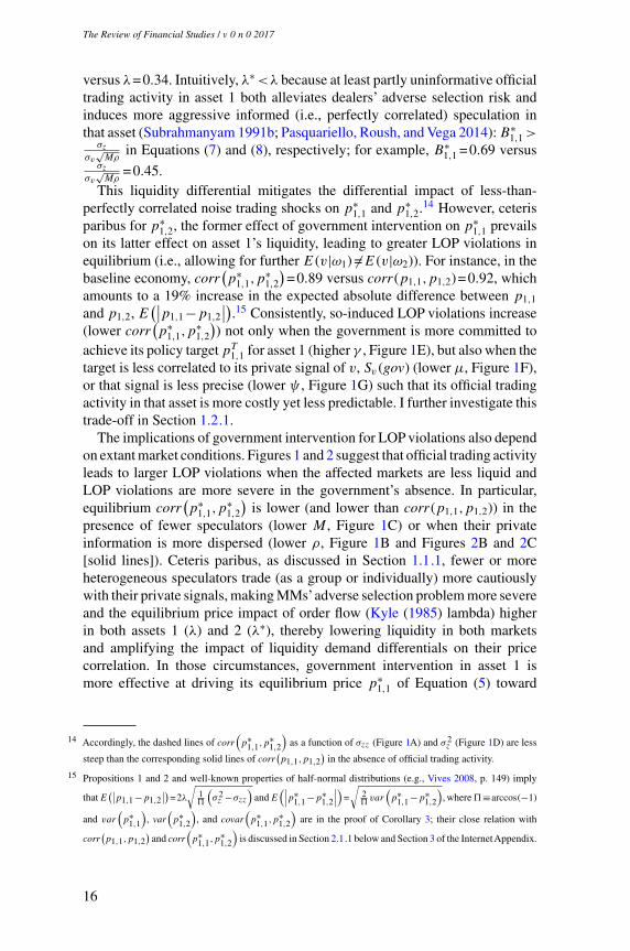
Figures 1 and 2 illustrate the intuition behind Corollary 1. I consider abaseline economy in which σ 2

v =1, σ 2z =1, σzz=0.5, ρ =0.5, and M =10. I then

plot the equilibrium price correlation of Equation (3) as a function of σzz, ρ,M , or σ 2

z in Figures 1A to 1D, respectively (solid lines). Figure 2A displays

7 For example,∂∣∣xi (m)

∣∣∂ρ

= σz2σv

√Mρ

>0, whereas∂

∣∣∣∑Mm=1xi (m)

∣∣∣∂M

=σz

∣∣v−p0∣∣

2σv√M

>0 in the limiting case in which

ρ =1; see also Pasquariello and Vega (2007). Accordingly, ∂λ∂ρ

=− σvM[(M−1)ρ−2]2σz

√Mρ[2+(M−1)ρ]2

<0 and ∂λ∂M

=

− σvρ[(M−1)ρ−2]2σz

√Mρ[2+(M−1)ρ]2

<0, except in the small region of {M,ρ} in which ρ≤ 2M−1 . In addition, ∂λ

∂σ2v

=√Mρ

2σvσz[2+(M−1)ρ] >0 and ∂λ∂σz

=− σv√Mρ

2σ3z [2+(M−1)ρ]

<0.

8

[14:52 19/7/2017 RFS-hhx074.tex] Page: 9 1–65


A B

C D

E F

G H

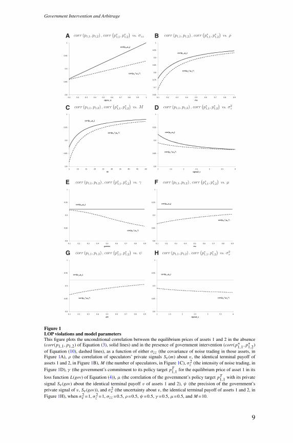
Figure 1LOP violations and model parametersThis figure plots the unconditional correlation between the equilibrium prices of assets 1 and 2 in the absence(corr(p1,1,p1,2) of Equation (3), solid lines) and in the presence of government intervention (corr(p∗

1,1,p∗1,2)

of Equation (10), dashed lines), as a function of either σzz (the covariance of noise trading in those assets, inFigure 1A), ρ (the correlation of speculators’ private signals Sv (m) about v, the identical terminal payoff ofassets 1 and 2, in Figure 1B), M (the number of speculators, in Figure 1C), σ2

z (the intensity of noise trading, in

Figure 1D), γ (the government’s commitment to its policy target pT1,1 for the equilibrium price of asset 1 in its

loss function L(gov) of Equation (4)), μ (the correlation of the government’s policy target pT1,1 with its privatesignal Sv (gov) about the identical terminal payoff v of assets 1 and 2), ψ (the precision of the government’sprivate signal of v, Sv (gov)), and σ2

v (the uncertainty about v, the identical terminal payoff of assets 1 and 2, inFigure 1H), when σ2

v =1, σ2z =1, σzz =0.5, ρ =0.5, ψ =0.5, γ =0.5, μ=0.5, and M =10.

9

[14:52 19/7/2017 RFS-hhx074.tex] Page: 10 1–65


A B

C

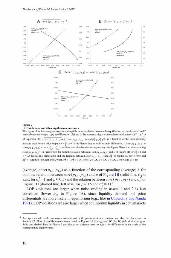
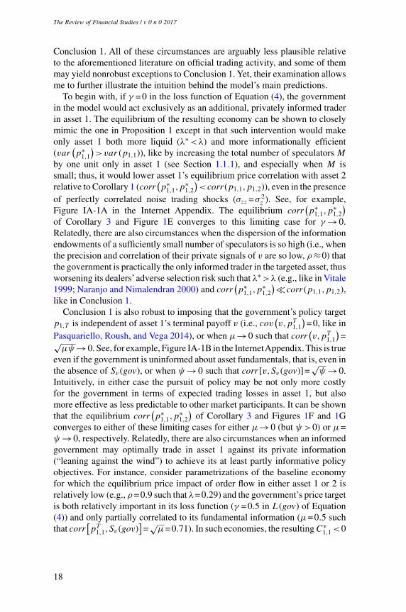
Figure 2LOP violations and other equilibrium outcomesThis figure plots the average unconditional equilibrium correlation between the equilibrium prices of assets 1 and 2in the absence (corr(p1,1,p1,2) of Equation (3)) and in the presence of government intervention (corr(p∗

1,1,p∗1,2)

of Equation (10)), corr(p1,1,p1,2)= 12 [corr(p1,1,p1,2)+corr(p∗

1,1,p∗1,2)], as a function of the corresponding

average equilibrium price impact λ= 12 (λ+λ∗) (in Figure 2A) as well as their difference, �corr(p1,1,p1,2)≡

corr(p1,1,p1,2)−corr(p∗1,1,p

∗1,2), as a function of either the corresponding λ (in Figure 2B) or the corresponding

corr(p1,1,p1,2) (in Figure 2C), for both the relation between corr(p1,1,p1,2) and ρ of Figure 1B for σ2z =1 and

ρ≈0.5 (solid line, right axis) and the relation between corr(p1,1,p1,2) and σ2z of Figure 1D for ρ =0.5 and

σ2z ≈1 (dashed line, left axis), when σ2

v =1, σ2z =1, σzz =0.5, ρ =0.5, ψ =0.5, γ =0.5, μ=0.5, and M =10.

(average) corr (p1,1,p1,2) as a function of the corresponding (average) λ forboth the relation between corr (p1,1,p1,2) and ρ of Figure 1B (solid line, rightaxis, for σ 2

z =1 and ρ≈0.5) and the relation between corr (p1,1,p1,2) and σ 2z of

Figure 1D (dashed line, left axis, for ρ =0.5 and σ 2z ≈1).8

LOP violations are larger when noise trading in assets 1 and 2 is lesscorrelated (lower σzz in Figure 1A), since liquidity demand and pricedifferentials are more likely in equilibrium (e.g., like in Chowdhry and Nanda1991). LOPviolations are also larger when equilibrium liquidity in both markets

8 Averages include both economies without and with government intervention; see also the discussion inSection 1.2. Plots of equilibrium outcomes based on Figures 1A (for σzz) and 1C (for M) yield similar insights.Solid and dashed lines in Figure 2 are plotted on different axes to adjust for differences in the scale of thecorresponding equilibriums.

10

[14:52 19/7/2017 RFS-hhx074.tex] Page: 11 1–65


is lower (i.e., the higher is λ), since the impact of noise trading on equilibriumprices is greater and the price differentials stemming from liquidity demanddifferentials in Equation (1) are larger. Thus, corr (p1,1,p1,2) is greater whenthere are fewer speculators in the economy (lower M in Figure 1B) or whentheir private information is more dispersed (lower ρ in Figures 1C and 2A),since the more cautious is their (aggregate or individual) trading activity and themore serious is the threat of adverse selection for MMs.9 Lastly, more intensenoise trading (higher σ 2

z in Figures 1D and 2A) amplifies LOP violations byincreasing both the likelihood and magnitude of liquidity demand differentials,despite its lesser impact (via lower λ) on equilibrium prices. I summarize theseobservations in Corollary 2.

Corollary 2. LOPviolations increase in speculators’information heterogene-ity and the intensity of noise trading, as well as decrease in the number ofspeculators and the covariance of noise trading.

LOP violations do not necessarily imply riskless arbitrage opportunities.While the former occur whenever nonzero price differences between two assetswith identical liquidation value arise, the latter require that those differencesbe exploitable with no risk. In my setting, only speculators can and do tradestrategically and simultaneously in both assets 1 and 2 (see Equation (2)).Hence, only they can attempt to profit from any price difference they anticipateto observe. However, the unconditional expected prices of assets 1 and 2 areidentical in equilibrium (E (p1,1)=E (p1,2)) since, by Condition 2, bothp1,1 andp1,2 incorporate all individual private information about their identical terminalvalue v (i.e., all private signals Sv (m) in Equation (1)). Further, speculatorscannot place limit orders and, in the noisy REE of Proposition 1, neitherobserve nor can accurately predict the market-clearing prices of assets 1 and 2when submitting their market orders, xi (m). Thus, there is no feasible risklessarbitrage opportunity in the economy.10

Segmentation in market making, speculative market-order trading, and less-than-perfectly correlated noise trading in the basic model are a reduced-formrepresentation of existing forces affecting the ability of financial markets tocorrectly price assets that are fundamentally linked by an arbitrage parity.

1.2 Government interventionGovernments often intervene in financial markets. The trading activity ofcentral banks and various governmental agencies has been argued and shownboth to affect price levels and dynamics of exchange rates, sovereign bonds,

9 However, greater fundamental uncertainty (higher σ2v ) does not affect corr

(p1,1,p1,2

), since lower market

liquidity is offset by greater price volatility in Equation (3).

10 See also the discussions in Subrahmanyam (1991a), Shleifer and Vishny (1997), and Pasquariello and Vega(2009).

11

[14:52 19/7/2017 RFS-hhx074.tex] Page: 12 1–65


derivatives, and stocks, as well as to yield often conflicting microstructureexternalities. Recent studies include Bossaerts and Hillion (1991), Dominguezand Frankel (1993), Bhattacharya and Weller (1997), Vitale (1999), Naranjoand Nimalendran (2000), Lyons (2001), Dominguez (2003), 2006), Evans andLyons (2005), and Pasquariello (2007b, 2010) for the spot and forward currencymarkets, Harvey and Huang (2002), Ulrich (2010), Brunetti, di Filippo, andHarris (2011), D’Amico and King (2013), Pasquariello, Roush, and Vega(2014), and Pelizzon et al. (2016) for the money and bond markets, and Sojliand Tham (2010) and Dyck and Morse (2011) for the stock markets.11 As such,this “official” trading activity may have an impact on the ability of the affectedmarkets to price assets correctly. I explore this possibility by introducing astylized government in the multiasset economy of Section 1.1.

The literature identifies several recurring features of direct governmentintervention in financial markets (e.g., Edison 1993; Vitale 1999; Sarno andTaylor 2001; Neely 2005; Menkhoff 2010; Engel 2014; Pasquariello, Roush,and Vega 2014): (1) governments tend to pursue nonpublic price targets in thosemarkets; (2) governments often intervene in secret in the targeted markets; (3)governments are likely or perceived to have an information advantage overmost market participants about the fundamentals of the traded assets; (4) theobserved ex post effectiveness of governments at pursuing their price targetsis often attributed to that actual or perceived information advantage; (5) thoseprice targets may be related to governments’ fundamental information; and(6) governments are sensitive to the potential costs of their interventions. Iparsimoniously capture these features using the following assumptions aboutthe stylized government.

First, the government is given a private and noisy signal of v, Sv (gov), anormally distributed variable with mean p0, variance σ 2

gov = 1ψσ 2v , and precision

ψ ∈ (0,1). I further impose that cov[Sv (m),Sv (gov)]=cov[v,Sv (gov)]=σ 2v ,

as for speculators’ private signals Sv (m) in Section 1.1. Accordingly, thegovernment’s information endowment about v is defined as δv (gov)≡E [v|Sv (gov)]−p0 =ψ [Sv (gov)−p0].

Second, the government is given a nonpublic target for the price ofasset 1, pT1,1, drawn from a normal distribution with mean pT1,1 andvariance σ 2

T . The government’s information endowment about pT1,1 is thenδT (gov)≡pT1,1 −pT1,1.12 This policy target is some unspecified functionof Sv (gov), such that σ 2

T = 1μσ 2gov = 1

μψσ 2v , cov

[pT1,1,Sv (gov)

]=σ 2

gov, and

11 However, direct government intervention in stock markets is currently less common, and evidence of this activityremains largely anecdotal. For example, see media coverage of the actions by the Chinese government in supportof the plunging Shanghai Composite Index in 2015 (Hong 2016). Other studies focus on the implications ofgovernment policies affecting the fundamental payoffs of traded securities for financial market outcomes (e.g.,Pastor and Veronesi 2012, 2013; Bond and Goldstein 2015).

12 In a model of currency trading based on Kyle (1985), Vitale (1999) shows that central bank intervention cannoteffectively achieve an uninformative price target known to all market participants.

12

[14:52 19/7/2017 RFS-hhx074.tex] Page: 13 1–65


cov[Sv (m),pT1,1

]=cov

(v,pT1,1

)=σ 2

v . Hence, when μ∈ (0,1) is higher, thegovernment’s price target is more correlated to its fundamental informationand market participants are less uncertain about its policy. For example, thisassumption captures the observation that government interventions in currencymarkets either “chase the trend” (if μ is high) to reinforce market participants’beliefs about fundamentals as reflected by observed exchange rate dynamics(e.g., Edison 1993; Sarno and Taylor 2001; Engel 2014) or more often “leanagainst the wind” (if μ is low) to resist those beliefs and dynamics (e.g.,Lewis 1995; Kaminsky and Lewis 1996; Bonser-Neal, Roley, and Sellon 1998;Pasquariello 2007b).13

Third, the government can only trade in asset 1; at date t =1, before theequilibrium price p1,1 has been set, it submits to the MMs a market orderx1 (gov) minimizing the expected value of its loss function:

L(gov)=γ(p1,1 −pT1,1

)2+(1−γ )(p1,1 −v)x1 (gov), (4)

where γ ∈ (0,1). This specification is based on Stein (1989), Bhattacharya andWeller (1997), Vitale (1999), and Pasquariello, Roush, and Vega (2014). Thefirst term in Equation (4) is meant to capture the government’s attempts toachieve its policy objectives for asset 1 by trading to minimize the squareddistance between asset 1’s equilibrium price, p1,1, and the target, pT1,1. Thesecond term in Equation (4) accounts for the costs of that intervention, namely,deviating from pure profit-maximizing speculation in asset 1 (γ =0). Whenγ is higher, the government is more committed to policy making in asset 1,relative to its cost. Imposing that γ <1 then ensures that the government doesnot implausibly trade unlimited amounts of asset 1 in pursuit of pT1,1. Thisfeature of Equation (4) is further discussed in Section 1.2.1.

At date t =1, MMs in each asset i clear their market after observing itsaggregate order flow,ωi , like in Section 1.1. However, whileω2 =

∑Mm=1x2 (m)+

z2, ω1 now consists of the market orders of noise traders, speculators, and thegovernment: ω1 =x1 (gov)+

∑Mm=1x1 (m)+z1. In this amended economy, MMs

in each asset i attempt to learn fromωi about that asset’s terminal payoff vwhensetting its equilibrium price p1,i , like in Section 1.1. However, each speculatornow uses her private signal, Sv (m), to learn not only about v and the otherspeculators’private signals but also about the government’s intervention policyin asset 1 before choosing her optimal trading strategy, xi (m), in both assets 1and 2. In addition, the government uses its private information, Sv (gov), to learnabout what speculators may know about v and trade in asset 1 when choosingits optimal intervention strategy, x1 (gov). I solve for the ensuing unique linearBayesian Nash equilibrium in Proposition 2.

13 Accordingly, in their REE model of currency trading, Bhattacharya and Weller (1997) also assume that the centralbank’s nonpublic price target is partially correlated to the payoff of the traded asset, forward exchange rates.

13

[14:52 19/7/2017 RFS-hhx074.tex] Page: 14 1–65


Proposition 2. There exists a unique linear equilibrium given by the pricefunctions:

p∗1,1 =

[p0 +2dλ∗(p0 −pT1,1

)]+λ∗ω1, (5)

p∗1,2 =p0 +λω2, (6)

where d = γ

1−γ , λ∗ is the unique positive real root of the sextic polynomial of

Equation (A33) in the Appendix, and λ= σv√Mρ

σz[2+(M−1)ρ] >0 (like in Proposition1); by each speculator’s orders

x∗1 (m)=B∗

1,1δv (m), (7)

x∗2 (m)=

σz

σv√Mρ

δv (m), (8)

where B∗1,1 = 2−ψ

λ∗{2[2+(M−1)ρ](1+dλ∗)−Mρψ(1+2dλ∗)}>0; and by the governmentintervention:

x1 (gov)=2d(pT1,1 −p0

)+C∗

1,1δv (gov)+C∗2,1δT (gov), (9)

where C∗1,1 =

[2+(M−1)ρ](1+dλ∗)−Mρ(1+2dλ∗)λ∗(1+dλ∗){2[2+(M−1)ρ](1+dλ∗)−Mρψ(1+2dλ∗)} and C∗

2,1 = d1+dλ∗ >0.

In Corollary 3, I examine the effect of government intervention in asset 1,x1 (gov) of Equation (9), on the extent of LOP violations in the economy (i.e.,on the unconditional comovement of equilibrium asset prices p∗

1,1 and p∗1,2 of

Equations (5) and (6)), like in Corollary 1.

Corollary 3. In the presence of government intervention, the unconditionalcorrelation of the equilibrium prices of assets 1 and 2 is given by:

corr(p∗1,1,p

∗1,2)=

σzz+σzσv√Mρ{B∗

1,1[1+(M−1)ρ]+ψC∗1,1 +C∗

2,1}σz

√[2+(M−1)ρ]{σ 2

z +σ 2v {MρB∗2

1,1[1+(M−1)ρ]+D∗1 +E∗

1 }},

(10)where D∗

1 =2Mρ[B∗

1,1

(ψC∗

1,1 +C∗2,1

)]and E∗

1 =ψC∗21,1 + 1

μψC∗2

2,1 +2C∗1,1C

∗2,1.

There are no LOP violations under perfectly integrated market making.

In the above economy, the equilibrium price impact of order flow inasset 1 (λ∗ of Proposition 2) cannot be solved in closed form (see theAppendix). Thus, I characterize the equilibrium properties of corr

(p∗

1,1,p∗1,2

)of Equation (10) via numerical analysis. To that purpose, I introduce thestylized government, with starting parameters γ =0.5, ψ =0.5, and μ=0.5, inthe baseline economy of Section 1.1.2, where σ 2

v =1, σ 2z =1, σzz=0.5, ρ =0.5,

andM =10. Most parameter selection only affects the relative magnitude of theeffects described below. I examine limiting cases and nonrobust exceptions of

14

[14:52 19/7/2017 RFS-hhx074.tex] Page: 15 1–65


interest in Section 1.2.1; see also the discussion in the proof of Proposition2. I then plot the ensuing equilibrium price correlation corr

(p∗

1,1,p∗1,2

)in

Figure 1 (dashed lines), alongside its corresponding level in the absenceof government intervention (corr (p1,1,p1,2) of Equation (3), solid lines), asa function of σzz, ρ, M , or σ 2

z (Figures 1A to 1D, like in Section 1.1.2),and γ , μ, ψ , or σ 2

v (Figure 1E to 1H). Figures 2B and 2C display theirdifference,�corr (p1,1,p1,2)≡corr (p1,1,p1,2)−corr

(p∗

1,1,p∗1,2

), as a function

of the corresponding average λ (i.e., λ= 12 (λ+λ∗)) and corr (p1,1,p1,2) (i.e.,

corr (p1,1,p1,2)= 12

[corr (p1,1,p1,2)+corr

(p∗

1,1,p∗1,2

)]), respectively, for both

their relation with ρ of Figure 1B (solid line, right axis, for σ 2z =1 and ρ≈0.5)

and their relation with σ 2z of Figure 1D (dashed line, left axis, for ρ =0.5 and

σ 2z ≈1).Like in Corollary 1, if MMs observe order flow in both assets 1 and

2, once again no LOP violation can arise in equilibrium under semi-strongmarket efficiency, regardless of government intervention: corr

(p∗

1,1,p∗1,2

)=

corr (p1,1,p1,2)=1. However, insofar as the dealership sector is segmented andmultiasset speculators submit market orders (i.e., ceteris paribus for existinglimits to arbitrage), government intervention makes LOP violations more likelyin equilibrium, even in the absence of liquidity demand differentials.Accordingto Figure 1, official trading activity in asset 1 lowers the unconditionalcorrelation of the equilibrium prices of the otherwise identical assets 1 and2 (i.e., corr

(p∗

1,1,p∗1,2

)<corr (p1,1,p1,2)) even when noise trading in those

assets is perfectly correlated (i.e., σzz=σ 2z =1 such that corr (p1,1,p1,2)=1 in

Figure 1A). Intuitively, the camouflage provided by the aggregate order flowallows the stylized government of Equation (4) to trade in asset 1 to pushits equilibrium price p∗

1,1 toward a target p1,T that is at most only partiallyinformative about fundamentals, that is, only partially correlated with bothassets’ identical terminal payoff v: corr

(v,pT1,1

)=

√μψ<1 (see also Vitale

1999; Naranjo and Nimalendran 2000). To that end, the government optimallychooses to bear some costs, that is, to tolerate some trading losses or foregosome trading profits in asset 1, given its private information of precision ψ .For instance, at the economy’s baseline parametrization, not only is C∗

2,1>0but also 0<C∗

1,1<B∗1,1 in x1 (gov) of Equation (9): C∗

2,1 =0.85 and C∗1,1 =0.34

versus B∗1,1 =0.69 in x∗

1 (m) of Equation (7).

Since pT1,1 is also nonpublic (i.e., policy uncertainty σ 2T = σ 2

v

μψ>0), the

uninformed MMs in asset 1 cannot fully account for the government’s tradingactivity when setting p∗

1,1 from the observed aggregate order flow in that asset,ω1 (i.e., E (v|ω1)). As such, camouflaged government intervention in asset 1is at least partly effective at pushing that asset’s equilibrium price p∗

1,1 toward

its partly uninformative policy target pT1,1—ceteris paribus,∂p∗

1,1

∂pT1,1= dλ∗

1+dλ∗ >0 in

Proposition 2—hence away from the equilibrium price of asset 2, p∗1,2, despite

occurring in a deeper market. For instance, in the baseline economy, λ∗ =0.18

15

[14:52 19/7/2017 RFS-hhx074.tex] Page: 16 1–65


versus λ=0.34. Intuitively, λ∗<λ because at least partly uninformative officialtrading activity in asset 1 both alleviates dealers’ adverse selection risk andinduces more aggressive informed (i.e., perfectly correlated) speculation inthat asset (Subrahmanyam 1991b; Pasquariello, Roush, and Vega 2014):B∗

1,1>σz

σv√Mρ

in Equations (7) and (8), respectively; for example, B∗1,1 =0.69 versus

σzσv

√Mρ

=0.45.This liquidity differential mitigates the differential impact of less-than-

perfectly correlated noise trading shocks on p∗1,1 and p∗

1,2.14 However, ceterisparibus for p∗

1,2, the former effect of government intervention on p∗1,1 prevails

on its latter effect on asset 1’s liquidity, leading to greater LOP violations inequilibrium (i.e., allowing for further E (v|ω1) �=E (v|ω2)). For instance, in thebaseline economy, corr

(p∗

1,1,p∗1,2

)=0.89 versus corr (p1,1,p1,2)=0.92, which

amounts to a 19% increase in the expected absolute difference between p1,1

and p1,2, E(∣∣p1,1 −p1,2

∣∣).15 Consistently, so-induced LOP violations increase(lower corr

(p∗

1,1,p∗1,2

)) not only when the government is more committed to

achieve its policy targetpT1,1 for asset 1 (higher γ , Figure 1E), but also when thetarget is less correlated to its private signal of v, Sv (gov) (lower μ, Figure 1F),or that signal is less precise (lower ψ , Figure 1G) such that its official tradingactivity in that asset is more costly yet less predictable. I further investigate thistrade-off in Section 1.2.1.

The implications of government intervention for LOP violations also dependon extant market conditions. Figures 1 and 2 suggest that official trading activityleads to larger LOP violations when the affected markets are less liquid andLOP violations are more severe in the government’s absence. In particular,equilibrium corr

(p∗

1,1,p∗1,2

)is lower (and lower than corr (p1,1,p1,2)) in the

presence of fewer speculators (lower M , Figure 1C) or when their privateinformation is more dispersed (lower ρ, Figure 1B and Figures 2B and 2C[solid lines]). Ceteris paribus, as discussed in Section 1.1.1, fewer or moreheterogeneous speculators trade (as a group or individually) more cautiouslywith their private signals, making MMs’adverse selection problem more severeand the equilibrium price impact of order flow (Kyle (1985) lambda) higherin both assets 1 (λ) and 2 (λ∗), thereby lowering liquidity in both marketsand amplifying the impact of liquidity demand differentials on their pricecorrelation. In those circumstances, government intervention in asset 1 ismore effective at driving its equilibrium price p∗

1,1 of Equation (5) toward

14 Accordingly, the dashed lines of corr(p∗

1,1,p∗1,2

)as a function of σzz (Figure 1A) and σ2

z (Figure 1D) are less

steep than the corresponding solid lines of corr(p1,1,p1,2

)in the absence of official trading activity.

15 Propositions 1 and 2 and well-known properties of half-normal distributions (e.g., Vives 2008, p. 149) imply

thatE(∣∣p1,1 −p1,2

∣∣)=2λ

√1�

(σ2z −σzz

)andE

(∣∣∣p∗1,1 −p∗

1,2

∣∣∣)=

√2�var

(p∗

1,1 −p∗1,2

), where�≡arccos(−1)

and var(p∗

1,1

), var

(p∗

1,2

), and covar

(p∗

1,1,p∗1,2

)are in the proof of Corollary 3; their close relation with

corr(p1,1,p1,2

)and corr

(p∗

1,1,p∗1,2

)is discussed in Section 2.1.1 below and Section 3 of the InternetAppendix.

16

[14:52 19/7/2017 RFS-hhx074.tex] Page: 17 1–65


the partially uninformative policy target, pT1,1—ceteris paribus,∂2p∗

1,1

∂pT1,1∂λ∗ =

d

(1+dλ∗)2 >0—hence farther away from the equilibrium price of asset 2 (p∗1,2

of Equation (6)).This effect, however, is less pronounced in correspondence with greater

fundamental uncertainty (higher σ 2v , Figure 1H). When private fundamental

information is more valuable, both market liquidity deteriorates (seeSection 1.1.1) and the pursuit of policy motives becomes more costly forthe government in the loss function of Equation (4). The latter partlyoffsets the former, leading to a nearly unchanged corr

(p∗

1,1,p∗1,2

). Similarly,

Figures 1 and 2 also suggest that government intervention may amplify LOPviolations more conspicuously (greater�corr (p1,1,p1,2)>0) even when thoseviolations are not as severe in its absence (high corr (p1,1,p1,2)). This mayoccur when noise trading in assets 1 and 2 (z1 and z2) is less intense,lowering liquidity in both markets (lower σ 2

z , Figure 1B and Figures 2Band 2C [dashed lines]), or when z1 and z2 are more positively correlated(higher σzz, Figure 1A). For instance, in the baseline economy with perfectlycorrelated noise trading shocks (σzz=σ 2

z =1), corr(p∗

1,1,p∗1,2

)=0.93 (and

E(∣∣p∗

1,1 −p∗1,2

∣∣)=0.27) versus corr (p1,1,p1,2)=1 (and E(∣∣p1,1 −p1,2

∣∣)=0).Hence, the observed relation between the impact of government interventionon LOP violations and their extant severity may be positive, negative,or possibly nonmonotonic. I summarize these novel, robust observationsabout the impact of government intervention on the LOP in Conclusions 1and 2.16

Conclusion 1. Under less-than-perfectly integrated market making, govern-ment intervention results in greater LOP violations in equilibrium, even in theabsence of liquidity demand differentials.

Conclusion 2. Government-induced LOP violations increase in the govern-ment’s policy commitment, speculators’ information heterogeneity, policy (butnot fundamental) uncertainty, and the covariance of noise trading, as well asdecrease in the quality of the government’s private fundamental information,the covariance of its policy target with fundamentals, the number of speculators,and the intensity of noise trading.

1.2.1 Limiting cases and exceptions. In this section, I examine theimplications of notable limiting cases of the model of Section 1.2 for the positiverelation between government intervention and LOP violations postulated in

16 As noted for the economy of Section 1.1, despite this impact, the unconditional expected prices of assets 1 and

2 remain identical (E(p∗

1,1

)=E

(p∗

1,2

)) and no feasible riskless arbitrage opportunity arises in equilibrium.

17

[14:52 19/7/2017 RFS-hhx074.tex] Page: 18 1–65


Conclusion 1. All of these circumstances are arguably less plausible relativeto the aforementioned literature on official trading activity, and some of themmay yield nonrobust exceptions to Conclusion 1. Yet, their examination allowsme to further illustrate the intuition behind the model’s main predictions.

To begin with, if γ =0 in the loss function of Equation (4), the governmentin the model would act exclusively as an additional, privately informed traderin asset 1. The equilibrium of the resulting economy can be shown to closelymimic the one in Proposition 1 except in that such intervention would makeonly asset 1 both more liquid (λ∗<λ) and more informationally efficient(var

(p∗

1,1

)>var (p1,1)), like by increasing the total number of speculators M

by one unit only in asset 1 (see Section 1.1.1), and especially when M issmall; thus, it would lower asset 1’s equilibrium price correlation with asset 2relative to Corollary 1 (corr

(p∗

1,1,p∗1,2

)<corr (p1,1,p1,2)), even in the presence

of perfectly correlated noise trading shocks (σzz=σ 2z ). See, for example,

Figure IA-1A in the Internet Appendix. The equilibrium corr(p∗

1,1,p∗1,2

)of Corollary 3 and Figure 1E converges to this limiting case for γ →0.Relatedly, there are also circumstances when the dispersion of the informationendowments of a sufficiently small number of speculators is so high (i.e., whenthe precision and correlation of their private signals of v are so low, ρ≈0) thatthe government is practically the only informed trader in the targeted asset, thusworsening its dealers’adverse selection risk such that λ∗>λ (e.g., like in Vitale1999; Naranjo and Nimalendran 2000) and corr

(p∗

1,1,p∗1,2

)�corr (p1,1,p1,2),like in Conclusion 1.

Conclusion 1 is also robust to imposing that the government’s policy targetp1,T is independent of asset 1’s terminal payoff v (i.e., cov

(v,pT1,1

)=0, like in

Pasquariello, Roush, and Vega 2014), or when μ→0 such that corr(v,pT1,1

)=√

μψ→0. See, for example, Figure IA-1B in the InternetAppendix. This is trueeven if the government is uninformed about asset fundamentals, that is, even inthe absence of Sv (gov), or when ψ→0 such that corr [v,Sv (gov)]=

√ψ→0.

Intuitively, in either case the pursuit of policy may be not only more costlyfor the government in terms of expected trading losses in asset 1, but alsomore effective as less predictable to other market participants. It can be shownthat the equilibrium corr

(p∗

1,1,p∗1,2

)of Corollary 3 and Figures 1F and 1G

converges to either of these limiting cases for either μ→0 (but ψ>0) or μ=ψ→0, respectively. Relatedly, there are also circumstances when an informedgovernment may optimally trade in asset 1 against its private information(“leaning against the wind”) to achieve its at least partly informative policyobjectives. For instance, consider parametrizations of the baseline economyfor which the equilibrium price impact of order flow in either asset 1 or 2 isrelatively low (e.g., ρ =0.9 such that λ=0.29) and the government’s price targetis both relatively important in its loss function (γ =0.5 in L(gov) of Equation(4)) and only partially correlated to its fundamental information (μ=0.5 suchthat corr

[pT1,1,Sv (gov)

]=

√μ=0.71). In such economies, the resultingC∗

1,1<0

18

[14:52 19/7/2017 RFS-hhx074.tex] Page: 19 1–65


inx1 (gov) of Equation (9), whileB∗1,1>0 inx∗

1 (m) of Equation (7):C∗1,1 =−0.04

versus B∗1,1 =0.55.

Lastly, government intervention in asset 1 may reduce LOP violations inequilibrium when σzz is close to zero or negative (such that liquidity trading inthe fundamentally identical assets 1 and 2 is weakly or negatively correlated),or when both ψ and μ are close to one (such that a nearly fully informedgovernment is in pursuit of a nearly fully informative policy target). Inthose more extreme circumstances—but only under some market conditions,like a relatively large number of speculators, and even if the government isuninformed and/or in pursuit of an uninformative target—such interventionmay increase equilibrium price correlation (corr

(p∗

1,1,p∗1,2

)>corr (p1,1,p1,2)),

in exception to Corollary 1, by at least partly offsetting the impact of highlydivergent noise trading shocks on p∗

1,1. See, for example, Figure IA-1C in theInternet Appendix.

1.3 Empirical implicationsThe stylized model of Sections 1.1 and 1.2 represents a plausible channelthrough which direct government intervention may affect the relative prices offundamentally linked securities in markets with less-than-perfectly integrateddealership. This channel depends crucially on various facets of governmentpolicy and the information environment of those markets. Yet, measuring suchintervention characteristics and market conditions is challenging, and oftenunfeasible. Under these premises, I identify from Corollary 1, Proposition 2,Figures 1 and 2, and Conclusions 1 and 2 the following subset of plausiblytestable implications of official trading activity for relative mispricings: H1)government intervention does not affect extant LOP violations, if any, inmarkets with perfectly integrated dealership; H2) government interventioninduces, or increases extant LOP violations in markets with less-than-perfectlyintegrated dealership; H3) this effect is more pronounced when market liquidityis low; H4) this effect is more pronounced when information heterogeneityis high; and H5) this effect is more pronounced when government policyuncertainty is high.

2. Empirical Analysis

I test the implications of my model by analyzing the impact of governmentintervention in currency markets on the relative pricing ofAmerican DepositaryReceipts and other U.S. cross-listings (“ADRs” for brevity).AnADR is a dollar-denominated security, traded in the United States, representing ownership ofa pre-specified amount (“bundling ratio”) of stocks of a foreign company,denominated in a foreign currency, held on deposit at a U.S. depositary banks(e.g., Karolyi 1998, 2006). In Section 2.1, I motivate the use of this setting tothat purpose. I describe the data in Section 2.2. Sections 2.3 to 2.5 contain theeconometric analysis.

19

[14:52 19/7/2017 RFS-hhx074.tex] Page: 20 1–65


2.1 ADRs and forex intervention in the modelThe market for U.S. cross-listings (the “ADR market”) represents an idealsetting to test my model, since its interaction with the foreign exchange(“forex”) market is consistent in spirit with the model’s basic premises.

First, exchange rates and ADRs are fundamentally linked by an arbitrageparity. Depositary banks facilitate the convertibility between ADRs and theirunderlying foreign shares (Gagnon and Karolyi 2010) such that the unit priceof an ADR i, Pi,t , should at any time t be equal to the dollar (USD) price of thecorresponding amount (bundling ratio) qi of foreign shares, P LOP

i,t :

P LOPi,t =St,USD/FOR×qi×P FOR

i,t , (11)

where P FORi,t is the unit foreign stock price denominated in a foreign currency

FOR, and St,USD/FOR is the exchange rate between USD and FOR. I interpretthe fundamental commonality in the terminal payoffs of assets 1 and 2 in themodel (v1 and v2) as a stylized representation of the LOP relation betweencurrency and ADR markets in Equation (11). In particular, Equation (11)suggests that one can think of asset 1 as the exchange rate—with payoffv1 =v—traded in the forex market at a price p1,1 (i.e., St,USD/FOR); and ofasset 2 as an ADR—whose payoff v2 is a linear function of the exchange rate:v2 =a2 +b2v, where a2 =0 and b2 =qi×P FOR

i,t >0, that is, ceteris paribus for thecorresponding foreign stock price—traded in the U.S. stock market at a tildedprice p̃1,2 =b2p1,2 (i.e., Pi,t ). Ignoring the market for an ADR’s underlyingforeign shares is for simplicity only and without loss of generality. In Section 1and Figure IA-2 of the Internet Appendix, I show that extending the model toa third such asset—with payoff v3 such that the ADR’s log-linearized payoffv2 =a2 +v1 +v3, where a2 = ln(qi)—requires more involved analysis but yieldssimilar implications.

In the above setting, the LOP relation between actual (Pi,t ) and synthetic(P LOPi,t ) ADR prices in Equation (11) can then be represented by the

unconditional correlation between p̃1,2 and pLOP1,2 =b2p1,1, respectively (e.g.,

Gromb and Vayanos 2010), such that in equilibrium: corr(p̃1,2,p

LOP1,2

)=

corr (p1,1,p1,2) of Equation (3). Accordingly, I postulate in Conclusion 1that, ceteris paribus, government intervention in the forex market—that is,targeting the exchange ratep1,1—lowers the unconditional correlation betweenexchange rates and actual ADR prices—that is, between p1,1 and p̃1,2:corr

(p∗

1,1,p̃∗1,2

)=corr

(p∗

1,1,p∗1,2

)of Equation (10), such that corr

(p∗

1,1,p̃∗1,2

)<

corr(p̃1,2,p

LOP1,2

). Hence, forex intervention may yield larger price differentials

between actual and synthetic ADRs—that is, it lowers the unconditionalcorrelation between p̃1,2 and pLOP

1,2 : corr(p̃∗

1,2,pLOP∗1,2

)=corr

(p∗

1,1,p∗1,2

), such

that corr(p̃∗

1,2,pLOP∗1,2

)<corr

(p̃1,2,p

LOP1,2

).

Second, market making in currency and ADR markets is arguably less-than-perfectly integrated, in that market makers in one market are less likely todirectly observe, and set prices based on, trading activity in the other market

20

[14:52 19/7/2017 RFS-hhx074.tex] Page: 21 1–65


than within their own.17 I interpret segmented market making in assets 1 and 2in the model as a stylized representation of this observation. Third, as mentionedin Section 1.2, the stylized representation of the government in the model isconsistent with the consensus in the literature that government intervention incurrency markets, although typically secret and in pursuit of nonpublic policy,is often effective at moving exchange rates because it is deemed at least partlyinformative about fundamentals.18 Fourth, the same literature suggests thatforex intervention is unlikely to be motivated by relative mispricings in theADRmarket. This observation alleviates reverse causality concerns when estimatingand interpreting any empirical relation between government intervention andthe arbitrage parity of Equation (11). I further assess this and other potentialsources of endogeneity in Section 2.3.1.

Overall, according to the model, these features of currency andADR marketsraise the possibility that government intervention in the former may lead to LOPviolations in the latter, that is, to “ADR parity” (ADRP) violations. I measurethese violations as nonzero absolute log percentage differences, in basis points(bps), between actual (Pi,t ) and theoreticalADR prices (P LOP

i,t of Equation (11)):

ADRPi,t =∣∣ln(Pi,t )−ln

(P LOPi,t

)∣∣×10,000 (12)

(e.g., Gagnon and Karolyi 2010; Pasquariello, Roush, and Vega 2014), andassess their empirical relation with forex intervention in the reminder of thepaper.

2.1.1 Alternative model interpretations and measures of ADRP violations.My investigation of the effects of forex interventions on ADRP violationsis qualitatively unaffected when considering alternative interpretations of thetraded assets in the model, relative to actual and synthetic ADRs in Equation(11), or alternative measures of LOP violations both in the model and in theADR market, relative to their absolute price differentials in Equation (12).

To begin with, I show in Section 2 of the Internet Appendix that the linearityof asset payoffs and equilibrium prices in the model implies that one can alsothink of asset 1 as the actual exchange rate traded in the forex markets andof asset 2 as either: (1) an ADR-specific synthetic, or shadow exchange rateimplied by Equation (11) implicitly traded in the ADR market at S i,LOP

t,USD/FOR =

Pi,t×(qi×P FOR

i,t

)−1(e.g., Auguste et al. 2006; Eichler, Karmann, and Maltritz

2009); or (2) an actual ADR traded in the U.S. stock market at Pi,t implying asynthetic exchange rate Si,LOPt,USD/FOR. Although less common and intuitive, these

17 See Lyons (2001) and Gagnon and Karolyi (2010) for investigations of the microstructure of currency and ADRmarkets, respectively.

18 Recent examples include Bhattacharya and Weller (1997), Peiers (1997), Vitale (1999), Naranjo and Nimalendran(2000), Payne and Vitale (2003), and Pasquariello (2007b). See also the comprehensive surveys in Edison (1993),Sarno and Taylor (2001), Neely (2005), Menkhoff (2010), and Engel (2014).

21

[14:52 19/7/2017 RFS-hhx074.tex] Page: 22 1–65


representations of the LOP relation between currency and ADR markets areconceptually and empirically equivalent to the one discussed in Section 2.1since any violation of the ADR parity of Equation (11) yields both Pi,t �=P LOPi,t and St,USD/FOR �=Si,LOPt,USD/FOR—that is, not only the same equilibrium price

correlation in the model but also the same absolute percentage LOP violationin Equation (12).

In addition, as noted in Section 1.1.2, the notion of LOP violations inthe ADR market as nonzero unsigned relative, that is, log percentage, pricedifferentials ADRPi,t of Equation (12) is both common in the literature andconceptually equivalent to the notion of LOP violations as less-than-oneequilibrium unconditional price correlation corr (p1,1,p1,2) in the model. Forinstance, I show in Section 3 of the InternetAppendix that the expected absolutedifferential between equilibrium actual and synthetic ADR prices described inSection 2.1 (i.e., E

(∣∣p̃1,2 −pLOP1,2

∣∣)) is a, ceteris paribus decreasing, functionof their unconditional correlation whose scale depends on the magnitude ofthe ADR’s fundamental payoff. Both corr (p1,1,p1,2) and ADRPi,t are insteadprice-scale invariant and display similar comparative statics (see also Augusteet al. 2006; Pasquariello 2008; Gagnon and Karolyi 2010). Accordingly,the empirical analysis of several measures of the correlation between actualand synthetic ADR prices, although computationally less convenient than forADRPi,t in my setting, yields qualitatively similar inference. See, for example,Figure IA-3 and Tables IA-1 and IA-2 in the Internet Appendix.

2.2 DataFor the empirical investigation of my model, I construct a sample of ADRstraded in U.S. stock exchanges and official intervention activity in currencymarkets over the past three decades.

2.2.1 ADRs. I begin by obtaining from Thomson Reuters Datastream(Datastream) its entire sample of foreign stocks cross-listed in the UnitedStates between January 1, 1973 and December 31, 2009.19 Following standardpractice in the literature, I then remove ADRs trading over-the-counter(Level I), Securities and Exchange Commission (SEC) Regulation S shares,private placement ADRs (Rule 144A), and preferred shares. In addition, Ialso conservatively exclude any identifiable cross-listing with ambiguous,incomplete, or missing descriptive, listing, or pairing information in theDatastream sample. This leaves a subset of 410 viable Level II and LevelIII ADRs from developed and emerging countries (with bundling ratios qi) andmostly Canadian ordinary shares (ordinaries, with qi =1) listed on the three

19 I complement this sample with the directory of depositary receipts compiled by Bank of New York Mellon (BNYMellon), available at https://www.adrbnymellon.com/directory/dr-directory.

22

[14:52 19/7/2017 RFS-hhx074.tex] Page: 23 1–65


Table 1ADRP violations: Summary statistics

ADRP violations ADRP illiquidity

ADRPm ADRPzm �ADRPm �ADRPzm ILLIQm

Country (Currency) Nv Nu N Mean SD Mean SD Mean SD Mean SD Mean SD

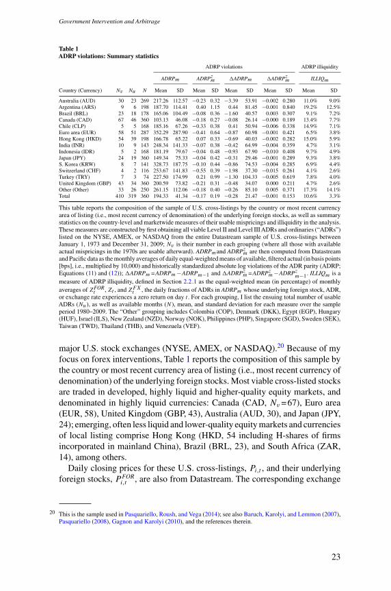
Australia (AUD) 30 23 269 217.26 112.57 −0.23 0.32 −3.39 53.91 −0.002 0.280 11.0% 9.0%Argentina (ARS) 9 6 198 187.70 114.41 0.40 1.15 0.44 81.45 −0.001 0.840 19.2% 12.5%Brazil (BRL) 23 18 178 165.06 104.49 −0.08 0.36 −1.60 40.57 0.003 0.307 9.1% 7.2%Canada (CAD) 67 46 360 103.13 46.08 −0.18 0.27 −0.08 26.14 −0.000 0.189 13.4% 7.7%Chile (CLP) 5 5 168 185.16 67.26 −0.33 0.38 0.41 50.94 −0.006 0.338 14.9% 7.1%Euro area (EUR) 58 51 287 352.29 287.90 −0.41 0.64 −0.87 60.98 −0.001 0.421 6.5% 3.8%Hong Kong (HKD) 54 39 198 166.78 65.22 0.07 0.33 −0.69 40.03 −0.002 0.282 15.0% 5.9%India (INR) 10 9 143 248.34 141.33 −0.07 0.38 −0.42 64.99 −0.004 0.359 4.7% 3.1%Indonesia (IDR) 5 2 168 181.19 79.67 −0.04 0.48 −0.93 67.90 −0.010 0.408 9.7% 4.9%Japan (JPY) 24 19 360 149.34 75.33 −0.04 0.42 −0.31 29.46 −0.001 0.289 9.3% 3.8%S. Korea (KRW) 8 7 141 328.73 187.75 −0.10 0.44 −0.86 74.53 −0.004 0.285 6.9% 4.4%Switzerland (CHF) 4 2 116 253.67 141.83 −0.55 0.39 −1.98 37.30 −0.015 0.261 4.1% 2.6%Turkey (TRY) 7 3 74 227.50 174.99 0.21 0.99 −1.30 104.33 −0.005 0.619 7.8% 4.0%United Kingdom (GBP) 43 34 360 200.59 73.82 −0.21 0.31 −0.48 34.07 0.000 0.211 4.7% 2.6%Other (Other) 33 26 250 261.15 112.06 −0.18 0.40 −0.26 85.10 0.005 0.371 17.3% 14.1%Total 410 319 360 194.33 41.34 −0.17 0.19 −0.28 21.47 −0.001 0.153 10.6% 3.3%

This table reports the composition of the sample of U.S. cross-listings by the country or most recent currencyarea of listing (i.e., most recent currency of denomination) of the underlying foreign stocks, as well as summarystatistics on the country-level and marketwide measures of their usable mispricings and illiquidity in the analysis.These measures are constructed by first obtaining all viable Level II and Level III ADRs and ordinaries (“ADRs”)listed on the NYSE, AMEX, or NASDAQ from the entire Datastream sample of U.S. cross-listings betweenJanuary 1, 1973 and December 31, 2009; Nv is their number in each grouping (where all those with availableactual mispricings in the 1970s are usable afterward). ADRPmand ADRPzm are then computed from Datastreamand Pacific data as the monthly averages of daily equal-weighted means of available, filtered actual (in basis points[bps], i.e., multiplied by 10,000) and historically standardized absolute log violations of the ADR parity (ADRP;Equations (11) and (12)); �ADRPm =ADRPm−ADRPm−1 and �ADRPzm =ADRPzm−ADRPz

m−1. ILLIQm is ameasure of ADRP illiquidity, defined in Section 2.2.1 as the equal-weighted mean (in percentage) of monthlyaverages of ZFOR

t , Zt , and ZFXt , the daily fractions of ADRs in ADRPm whose underlying foreign stock, ADR,or exchange rate experiences a zero return on day t . For each grouping, I list the ensuing total number of usableADRs (Nu), as well as available months (N), mean, and standard deviation for each measure over the sampleperiod 1980–2009. The “Other” grouping includes Colombia (COP), Denmark (DKK), Egypt (EGP), Hungary(HUF), Israel (ILS), New Zealand (NZD), Norway (NOK), Philippines (PHP), Singapore (SGD), Sweden (SEK),Taiwan (TWD), Thailand (THB), and Venezuela (VEF).

major U.S. stock exchanges (NYSE, AMEX, or NASDAQ).20 Because of myfocus on forex interventions, Table 1 reports the composition of this sample bythe country or most recent currency area of listing (i.e., most recent currency ofdenomination) of the underlying foreign stocks. Most viable cross-listed stocksare traded in developed, highly liquid and higher-quality equity markets, anddenominated in highly liquid currencies: Canada (CAD, Nv =67), Euro area(EUR, 58), United Kingdom (GBP, 43), Australia (AUD, 30), and Japan (JPY,24); emerging, often less liquid and lower-quality equity markets and currenciesof local listing comprise Hong Kong (HKD, 54 including H-shares of firmsincorporated in mainland China), Brazil (BRL, 23), and South Africa (ZAR,14), among others.

Daily closing prices for these U.S. cross-listings, Pi,t , and their underlyingforeign stocks, P FOR

i,t , are also from Datastream. The corresponding exchange

20 This is the sample used in Pasquariello, Roush, and Vega (2014); see also Baruch, Karolyi, and Lemmon (2007),Pasquariello (2008), Gagnon and Karolyi (2010), and the references therein.

23

[14:52 19/7/2017 RFS-hhx074.tex] Page: 24 1–65


rates in Equation (11), St,USD/FOR, are daily indicative spot mid-quotes, asobserved at 12 p.m. Eastern Standard Time (EST), from Pacific ExchangeRate Service (Pacific) and Datastream. Although commonly used, the resultingdataset allows to measure the extent of LOP violations in the ADR marketonly imprecisely (see, e.g., Ince and Porter 2006; Xie 2009; Gagnon andKarolyi 2010; Pasquariello, Roush, and Vega 2014). For instance, the tradinghours in many of the foreign stock and currency markets listed in Table 1are partly overlapping or nonoverlapping with those in New York, yieldingnonsynchronous closing prices. Individual ADRP violations often differ inscale, making cross-sectional comparisons problematic, and either persist ordisplay discernible trends. Paired closing foreign stock, currency, orADR pricesmay also be stale (e.g., reflecting sparse trading), incorrectly reported (e.g., dueto inaccurate data entry or around delistings), partly unavailable, or sometimesaltogether missing.

Pasquariello, Roush, and Vega (2014) proposes two measures of themarketwide (i.e., aggregate), low-frequency extent of violations of the ADRparity of Equation (11) addressing these concerns. The first measure, ADRPm,is the monthly average of daily equal-weighted means of all available, filteredrealizations of ADRPi,t of Equation (12), that is, of daily mean absolutepercentage ADRP violations. In particular, I conservatively remove from theseaverages any available ADRPi,t deemed “too large” (ADRPi,t >1,000 bps) orstemming from “too extreme” ADR prices (Pi,t <$5 or Pi,t >$1,000). Theserequirements and the aforementioned data limitations reduce the number ofusable ADRs to 319 in total and roughly uniformly across most groupingsin Table 1, except for Turkey (Nu=3), Indonesia (3), Hong Kong (39), andCanada (46).21 Yet, filtering and daily averaging across individual ADRsminimize the impact of any idiosyncratic parity violations (or lack thereof),for example, due to quoting errors, missing data, or other data issues in thesample. Monthly averaging further smooths any spurious daily variability inobserved ADRP violations, for example, due to bid-ask bounce, price staleness,nonsynchronicity, or data gaps, among others. The second measure, ADRPzm,is the monthly average of daily equal-weighted means of all historicallynormalized ADRP violations, ADRPzi,t—that is, after each usable realization ofADRPi,t has been standardized by its earliest available historical distributionon day t since 1973.22 Up-to-current normalization allows me to identifyindividual abnormal ADRP violations—that is, innovations in each observedADRPi,t relative to its time-varying, potentially spurious mean—without look-ahead bias, while making these violations comparable in scale across ADRs.

21 The analysis and inference are unaffected by this filtering procedure or by excluding all Canadian ordinaries,whose fungibility and propensity to delist from U.S. exchanges differ from those of ADRs and other ordinaries(Witmer 2008; Gagnon and Karolyi 2010).

22 Specifically, I standardize each available, filtered absolute ADR parity violation, ADRPi,t , by its historical meanand standard deviation over at least 22 observations up to (and including) its current realization.

24

[14:52 19/7/2017 RFS-hhx074.tex] Page: 25 1–65


A B

Figure 3ADRP violations and forex interventionThis figure plots the aggregate measures of LOP violations in the ADR market, defined in Section 2.2.1 as themonthly averages of daily equal-weighted means of available actual (ADRPm, Figure 3A, right axis, solid line,in basis points [bps], i.e., multiplied by 10,000) and standardized (ADRPzm, Figure 3B, right axis, solid line)absolute log violations of the ADR parity of Equation (11), as well as the aggregate measures of governmentintervention in the forex market, defined in Section 2.2.2 as the number of government intervention-exchangerates pairs in each monthm (Nm (gov), Figure 3A, left axis, histogram) and the number of those pairs standardizedby its historical distribution in month m (Nzm (gov), Figure 3B, left axis, dashed line), over the sample period1980–2009.

As such,ADRP zm is positive (higher) in correspondence with historically large(larger) LOP violations in the ADR market.

Foreign companies rarely issued ADRs before the 1980s (e.g., Karolyi 2006;Sarkissian and Schill 2016; Karolyi and Wu Forthcoming). When they did,their local and cross-listed stock prices in my sample—although frequentlyassociated with usable mispricings for all of them afterward—are often eitherstale or suspect then, yielding extreme LOP violations. Accordingly, thefiltering and aggregation procedure described above results in several missingobservations between 1973 and 1979. Thus, I focus the empirical analysis onthe interval 1980–2009, the longest portion of the sample with the greatestaggregate and country-level continuous coverage. Inference from the fullsample is qualitatively similar. Summary statistics for marketwide and country-level ADRPm and ADRPzm for the sample period 1980–2009 are in Table 1; theirmarketwide plots are in Figures 3A and 3B (right axis, solid line).

Consistent with the aforementioned literature, absolute ADR parityviolations ADRPm in the past three decades are large (e.g., a sample meanof nearly 2% [194 bps]). They are also volatile, although not exceedinglyso (e.g., a sample standard deviation of 41 bps), and declining, perhapsreflecting improving quality and integration of the world financial markets.Once controlling for this trend, scaled such violations (ADRP zm), while oftenstatistically significant, display more discernible cycles and spikes, especiallyduring periods of financial turmoil.23 Both measures also display nontrivial

23 In particular, ADRPzm is statistically significant at the 10% level in 76% of all months over the sample period1980–2009; ADRPzm is highest in October 2008, in correspondence with the global financial crisis initiated by

25

[14:52 19/7/2017 RFS-hhx074.tex] Page: 26 1–65


cross-country heterogeneity. LOP violations in Table 1 are on average mostpronounced for ADRs from Europe, Australia, and emerging markets (e.g.,Mexico, South Africa, and South Korea), and least pronounced for Canadianordinaries, which have long been trading synchronously and (as noted earlier)on a one-to-one basis in both Canada and the United States.

The model of Section 1 relates extant (corr (p1,1,p1,2)<1) and intervention-induced equilibrium LOP violations (corr

(p∗

1,1,p∗1,2

)<corr (p1,1,p1,2)) to

common, exogenous forces affecting the equilibrium liquidity of theunderlying, arbitrage-linked markets (λ and λ∗), such as the number ofmultiasset speculators (M , in Figure 1C) or the correlation of their privatefundamental information (ρ, in Figure 1B). In light of this observation,Equation (11) suggests that ADR parity violations may be related to exogenouscommonality in the liquidity of the U.S. stock market where an ADR isexchanged, the listing market for the underlying foreign stock, and thecorresponding currency market. Those violations may also be caused by suchilliquidity increasing the cost of ADR arbitrage activity (e.g., Gagnon andKarolyi 2010; Gromb and Vayanos 2010). Data availability considerationsmake measurement of liquidity in many of these venues over long sampleperiods challenging, especially in emerging markets (e.g., Lesmond 2005;Lyons and Moore 2009; Mancini, Ranaldo, and Wrampelmeyer 2013).Lesmond, Ogden, and Trzcinka (1999) and Lesmond (2005) propose to measurea security’s (or a market’s) illiquidity by its incidence of zero returns, as therelative frequency of its price changes may depend on transaction costs andother impediments to trade; they then show that so-constructed estimates arehighly correlated with popular measures of liquidity like quoted or effectivebid-ask spreads (when available; see also Bekaert, Harvey, and Lundblad 2007).

Accordingly, I define and compute composite marketwide and country-levelilliquidity measures, ILLIQm (Figure 4A), for both ADRPm andADRP zm as theequal-weighted means of monthly averages of ZFOR

t , Zt , and ZFXt —the dailyfractions of ADRs in the corresponding grouping whose underlying foreignstock, ADR, or exchange rate experiences a zero return on day t (P FOR

i,t =P FORi,t−1,

Pi,t =Pi,t−1, or St,USD/FOR =St−1,USD/FOR), respectively. This procedure allowsto capture any commonality in ADR parity-level liquidity parsimoniously, overthe full sample, and without look-ahead bias. Summary statistics for ILLIQm

(in percentage) are in Table 1. Perhaps unsurprisingly, the so-defined ADRPilliquidity of cross-listings from developed economies is lower than in emergingmarkets; for example, the average fraction of zero returns across U.S., foreignstock, and currency markets ILLIQm is as low as 4.1% for Switzerland and 4.7%for the United Kingdom, and as high as 19.2% for Argentina and 16.6% forMexico. However, there is also significant heterogeneity in ADRP illiquidityacross both sets of markets; for example, ILLIQm for cross-listings from South

Lehman Brothers’ default (on September 15, 2008). Qualitatively similar inference ensues from excluding thesubperiod 2008–2009 from the analysis.

26

[14:52 19/7/2017 RFS-hhx074.tex] Page: 27 1–65


Korea (6.9%) or Turkey (7.8%) is lower than for those from Canada (13.4%)or Australia (11%).

Interestingly, Table 1 further suggests that large ADRP violations tend tobe associated with both extremes of the cross-sectional distribution of ADRPilliquidity. For instance, mean ADRPm and ADRPzm are relatively high for cross-listings not only from Argentina and Mexico (whose ILLIQm are high) butalso from the Euro area and South Korea (whose ILLIQm is instead low).24

This preliminary observation is consistent with my model’s basic premise, assummarized in Corollary 2. In the basic model of multiasset trading withoutgovernment intervention of Section 1.1, LOP violations are likely to be larger(i.e., corr (p1,1,p1,2) is lower) not only when (the commonality in) assetliquidity is low—because the price impact of less-than-perfectly correlatednoise trading is greater—but also when it is high—because the intensity ofless-than-perfectly correlated noise trading is greater. See, for example, theplots of corr (p1,1,p1,2) versus λ in Figure 2A. I investigate this relation and,more generally, the relevance of extant market quality for the LOP externalityof government intervention, in greater detail in Sections 2.4 and 2.5.

2.2.2 Forex interventions. As noted earlier, the forex market is not only oneof the largest and deepest financial markets but also one where governmentinterventions occur most often.25 According to the literature (surveyed inEdison 1993; Sarno and Taylor 2001; Neely 2005; Menkhoff 2010; Engel2014), monetary authorities, like central banks, and other government agenciesfrequently engage in secret, generally small, nearly always sterilized currencytransactions (i.e., accompanied by offsetting actions on the domestic moneysupply), normally in a coordinated fashion, to accomplish their habituallynonpublic policy objectives for exchange rate dynamics, at least in the short-run, by virtue of their actual or perceived informativeness about marketfundamentals.

As discussed in Section 1.2, the stylized government of Equation (4) capturesin spirit those features of observed official currency trading activity. To measurethis activity, I use the database of government intervention in currency marketsavailable on the Federal Reserve Economic Data (FRED) website of the FederalReserve Bank of St. Louis.26 This database contains daily amounts of domesticand/or foreign currencies traded by the governments of Australia, Germany,Italy, Japan, Mexico, Switzerland, Turkey, and the United States for policy

24 Accordingly, Gagnon and Karolyi (2010) find that estimates of the price impact of order flow in the foreign(U.S.) stock market are positively related to relative ADR parity violations for cross-listings from markets withrelatively high (low) levels of economic and capital market development. See also Baruch, Karolyi, and Lemmon(2007) and Levy Yeyati, Schmukler, and Van Horen (2009).

25 For an overview of the main characteristics of the global currency markets, see the 2016 triennal survey by theBank for International Settlements (BIS 2016).

26 See https://fred.stlouisfed.org/categories/32145.

27

[14:52 19/7/2017 RFS-hhx074.tex] Page: 28 1–65


reasons—that is, to influence exchange rates—over the past several decades, insome cases as early as in 1973 or as late as in 2009.27 Where currency-specificintervention data are missing, I augment the FRED database using variousofficial government sources (when possible).28 As for the sample of ADRparity violations, the resulting sample has the broadest continuous coverageof currency intervention activity between 1980 and 2009.29

Panel A of Table 2 reports summary statistics for these interventions,aggregated at the monthly frequency over this period, by country and foreignexchange involved. All governments in the sample intervene by purchasingor selling their domestic currencies. Most often, they do so against USD, thecurrency of denomination of ADRs; less so via cross-rates, exchange rates notinvolving vehicle currencies like USD or EUR.30 Cross-rates are however keptin line with the corresponding USD-denominated exchange rates by triangulararbitrage (Bekaert and Hodrick 2012); thus, any intervention in the formermust reverberate in the latter. Excluding those interventions from the sampledoes not affect the inference; see, for example, Tables IA-3 and IA-4 in theInternet Appendix.

According to Table 2, and consistent with the aforementioned literature,the absolute amounts of currency traded by these governments in the sample,while nontrivial, are small relative to the average monthly trading volume in theforex market (e.g., USD 111 trillions, according to BIS 2016) and heterogeneousacross currencies and governments. Yet, scaling and aggregating these amountsis impeded by cross-currency turnover heterogeneity and sparsity of historicalcurrency turnover data. Furthermore, in my model, like in all models basedon Kyle (1985), optimal strategic and noise trading activity in general, andoptimal intervention intensity in particular (i.e., sign and magnitude of x1 (gov)of Equation (9)), are separately unobservable by dealers and endogenouslydetermined in equilibrium. However, the presence of an active governmentis exogenous and known to all market participants. Both the presence andoptimal intensity of an intervention contribute to its impact on equilibriumprice formation. Relatedly, the effect of x1 (gov) on equilibrium outcomesdepends not only on the realizations of unobservable variables controlling

27 Accordingly, as is standard, I remove from the sample all customer transactions, that is, central banks’ infrequentpassive forex trades triggered not by policy motives but by their domestic governments’ mundane requests forforeign currencies (e.g., Payne and Vitale 2003; Pasquariello 2007b).

28 More detailed information on the intervention activity of any of these governments (e.g., time-stamped tradesor transaction prices) is rarely available over extended sample periods, with the exception of the Swiss NationalBank (SNB; Fischer and Zurlinden 1999).

29 Official trades in the sample may have been executed in the spot and/or forward currency markets, although theformer is much more common than the latter (e.g., Neely 2000). Only in the case of Australia, the FRED databaseexplicitly mentions consolidating spot and forward transactions by the Reserve Bank of Australia (RBA).

30 Japan and Switzerland occasionally trade on exchange rates between foreign currencies and USD. In the case ofeither Italy and the United States or Germany, the FRED database also reports official trades in their domesticcurrencies relative to either unspecified “other” currencies or unspecified currencies in the European MonetarySystem (EMS).

28

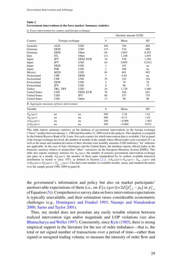
[14:52 19/7/2017 RFS-hhx074.tex] Page: 29 1–65


Table 2Government interventions in the forex market: Summary statistics

A. Forex intervention by country and foreign exchange

Absolute amount ($1M)

Country Foreign exchange N Mean SD

Australia AUD USD 184 394 460Germany DEM USD 115 534 688Germany DEM Other 66 2,603 8,293Italy ITL Other 111 1,168 1,655Japan JPY DEM, EUR 10 930 1,296Japan JPY USD 64 9,092 12,012Japan DEM USD 1 101 naJapan INR USD 1 568 naMexico MXN USD 84 601 492Switzerland CHF DEM 1 0.44 naSwitzerland CHF USD 39 163 164Switzerland DEM USD 2 70 78Switzerland JPY USD 6 98 73Turkey TRL, TRY USD 16 1,728 1,460United States USD DEM, EUR 76 626 641United States USD JPY 60 537 755United States USD Other 12 90 88

B. Aggregate measures of forex intervention

Variable N Mean SD

Nm (gov) na na 360 2.36 1.61Nzm (gov) na na 360 −0.13 1.03�Nm (gov) na na 360 −0.006 1.402�Nzm (gov) na na 360 −0.004 0.911

This table reports summary statistics on the database of government interventions in the foreign exchange(“forex”) market between January 1, 1980 and December 31, 2009 used in the analysis. This database is compiledby the Federal Reserve Bank of St. Louis. For each country for which intervention data is available, I list in panelA the foreign exchange involved, the number of months in the sample when official trades were executed (N), aswell as the mean and standard deviation of their absolute total monthly amounts (USD millions); “na” indicatesnot applicable. In the case of Italy (Germany) and the United States, the database reports official trades in thedomestic currency relative to unspecified “other” currencies (in the European Monetary System [EMS]). Thistable also reports summary statistics for Nm (gov), the number of nonzero government intervention-exchangerate pairs in a month, Nzm (gov), the number of those pairs standardized by its earliest available historicaldistribution in month m since 1973, as defined in Section 2.2.2; �Nm (gov)=Nm (gov)−Nm−1 (gov) and�Nzm (gov)=Nzm (gov)−Nz

m−1 (gov). I list their total number of available months, mean, and standard deviationover the sample period 1980–2009 in panel B.

the government’s information and policy but also on market participants’unobservable expectations of them (i.e., on E [x1 (gov)]=2d

(pT1,1 −p0

)in p∗

1,1of Equation (5)). Comprehensive survey data on forex intervention expectationsis typically unavailable, and their estimation raises considerable econometricchallenges (e.g., Dominguez and Frankel 1993; Naranjo and Nimalendran2000; Sarno and Taylor 2001).

Thus, my model does not postulate any easily testable relation betweenrealized intervention sign and/or magnitude and LOP violations (see alsoBhattacharya and Weller 1997). Consistently, since Kyle (1985), there is strongempirical support in the literature for the use of order imbalance—that is, thetotal or net signed number of transactions over a period of time—rather thansigned or unsigned trading volume, to measure the intensity of order flow and

29

[14:52 19/7/2017 RFS-hhx074.tex] Page: 30 1–65


estimate its impact on price formation in financial markets (see, e.g., Hasbrouck1991, 2007; Jones, Kaul, and Lipson 1994; Evans and Lyons 2002; Chordiaand Subrahmanyam 2004; Green 2004; Pasquariello and Vega 2007; Chordiaet al. 2017).31

In addition, as mentioned above, most currency interventions are coordinatedamong multiple governments for greatest effectiveness (e.g., Dominguez andFrankel 1993; Sarno and Taylor 2001); however, individual transactions withina concerted forex policy may not be contemporaneous, as they are executedin different time zones and often coordinated through informal discussions.Accordingly, many of the official currency trades in Table 2 tend to cluster intime but often are not perfectly synchronous at high frequency. Lastly, Tables 1and 2 suggest that there is relative scarcity of currency-matched intervention-ADR pairs and events in the sample. For instance, forex interventions in Table 2can be feasibly matched to only 105 usable ADRs in Table 1 whose underlyingforeign stocks are denominated in the involved currencies (AUD, EUR, JPY,MXN, or TRY), and only over the portions of the sample period 1980–2009when both are contemporaneously available.32 Yet, portfolio rebalancing, pricepressure, and triangular arbitrage effects may induce significant cross-currencyspillovers of interventions involving vehicle currencies (e.g., Dominguez 2006;Beine, Bos, and Laurent 2007; Beine, Laurent, and Palm 2009; Chortareas,Jiang, and Nankervis 2013; Gerlach-Kristen, McCauley, and Ueda 2016).Analysis of this smaller dataset (in Section 2.4) yields noisier but qualitativelysimilar inference.

In light of these observations, I propose two aggregate, low-frequencymeasures of the presence and intensity of government intervention in the forexmarket. The first measure, Nm (gov), is the number of nonzero governmentintervention-exchange rates pairs in a month. The second measure, Nz

m (gov),is such a number standardized by its earliest available historical distributionin month m since 1973, as in Section 2.2.1. Hence, as for normalized ADRPviolations ADRPzm, a positive (negative)Nz

m (gov) indicates an abnormally large(small) number of government interventions—that is, historically high (low)intensity of official trading activity—in the forex market during month m.Consistent with the aforementioned literature, replacingNm (gov) andNz

m (gov)in the ensuing analysis with the actual and normalized sums of unsigned andunscaled observed government trades (in USD millions at concurrent exchangerates) yields similar but weaker evidence, while augmenting that analysis by

31 For instance, in their seminal empirical investigation of the U.S. stock market, Jones, Kaul, and Lipson (1994,p. 631) find that “it is the occurrence of transactions per se, and not their size, that generates [price] volatility;trade size has no information beyond that contained in the frequency [i.e., number] of transactions.” Accordingto Hasbrouck (2007, p. 90), time-averaged price formation is relatively unaffected by order size because of timevariation in liquidity since, like in my model, “agents trade large amounts when price impact is low, and smallamounts when price impact is high.”

32 For example, I observe no interventions in CHF or INR over the portions of the sample period when I cancompute ADRP violations for cross-listed stocks denominated in CHF or INR; in addition, USD interventionsby the United States in unspecified “other” currencies (see Table 2) cannot be matched to any ADR.

30

[14:52 19/7/2017 RFS-hhx074.tex] Page: 31 1–65


those measures does not affect the inference. See, for example, Figure IA-4Aand Tables IA-5 and IA-7 in the Internet Appendix.

I plotNm (gov) andNzm (gov) in Figures 3A (left axis, histogram) and 3B (left

axis, dashed line), alongside ADRPm and ADRPzm, respectively. Their summarystatistics are in panel B of Table 2. Forex interventions (i.e., Nm (gov)≥1 inFigure 3A) occur in almost every month of the sample; thus, identification oftheir impact on LOP violations may come from their time-varying intensity.Official trading activity in the currency markets is especially intense in thelate 1980s and mid-1990s, before abating afterward. In those circumstances,both Nm (gov) and Nz

m (gov) experience frequent sharp spikes, suggestingthat episodes of coordinated forex intervention are often short-lived but notisolated.33 Figure 3 also suggests that more frequent forex intervention isoften accompanied by larger LOP violations in the ADR market. I formallyinvestigate this possibility next.

2.3 Marketwide ADRP violationsTable 2 and Figure 3 indicate that the market for ADRs experiences nontrivialLOP violations between 1980 and 2009. According to the model of Section 1(see, e.g., H2 in Section 1.3), government intervention in currency marketsmay induce their occurrence or increase their intensity.

I test this prediction by specifying the following regression model for changesin monthly averages of measures of those LOP violations (e.g., Neely 2005;Pasquariello 2007b; Garleanu and Pedersen 2011):

�LOPm=α+β−1�Im−1 +β0�Im+β1�Im+1 +εm, (13)

where LOPm is either ADRPm or ADRPzm, �LOPm=LOPm−LOPm−1, Im iseither Nm (gov) or Nz

m (gov), and �Im=Im−Im−1. Both ADR parity violationsand the intensity of forex interventions tend to persist; for instance, thetime series of ADRPm and Nm (gov) in Figure 3A (ADRPzm and Nz

m (gov) inFigure 3B) have a first-order serial correlation of 0.86 and 0.62 (0.68 and0.61), respectively. Regressions in changes mitigate biases caused by potentialnon-stationarity (e.g., Hamilton 1994). In unreported analysis, regressions inlevels yield similar or stronger results. Year and month fixed effects (or linearand quadratic time trends) are nearly always statistically insignificant and theirinclusion does not affect the inference. The coefficient β0 in Equation (13)captures the contemporaneous impact of forex intervention activity (�Im>0)on ADRP violations (�LOPm) predicted by the model of Section 1.2 anddiscussed in Section 2.1, that is, �corr (p1,1,p1,2)>0 in Figures 1, 2B,and 2C. Currency market participants may anticipate the nature and/or extentof forex intervention and react prior to its actual occurrence (�Im+1>0), for

33 Nonetheless,Nzm (gov) is nearly always statistically significant, for example, at the 10% level in 91% of all monthsover the sample period 1980-2009.

31

[14:52 19/7/2017 RFS-hhx074.tex] Page: 32 1–65


instance, if its policy objectives and/or accompanying trades are pre-announcedby government officials or leaked to the media (Payne and Vitale 2003;Beine, Janssen, and Lecourt 2009). In Equation (13), the impact of any suchanticipation in currency markets on the LOP relation between current actualand synthetic ADR prices of Equation (11) is captured by the lead coefficientβ1. The effects of past forex intervention (�Im−1>0) on LOP violations in theADR market may persist or ebb, for example, depending on the extent to whichcurrency market participants learn about the government’s prior trades andpolicy objectives (Jansen and De Haan 2005; Fratzscher 2006). In Equation(13), the impact of any such persistence or reversal in currency markets oncurrent ADRP violations is captured by the lag coefficient β−1.

I estimate Equation (13) by ordinary least squares (OLS) over the sampleperiod 1980-2009 and report these coefficients, as well as their cumulativesums, β0

1 =β1 +β0 and β−11 =β1 +β0 +β−1, in panel A of Table 3.34 According to

Dimson (1979), estimates of β−11 can also be interpreted as correcting for any

bias in the contemporaneous coefficient β0 due to nonsynchronous or sparsetrading (e.g., price staleness).

The results in Table 3 provide support for the main prediction of my model(H2). Estimates of both the contemporaneous and up-to-current impact of forexinterventions on ADR parity violations are positive and statistically significant:β0>0 and β0

1 >0. These estimates are (plausibly) economically significant aswell. For example, a one-standard-deviation increase in the monthly change inthe number of forex interventions�Nm (gov)—1.402, in panel B of Table 2—isaccompanied by a contemporaneous (up-to-current) increase in average ADRparity violations ADRPm in (up to) that month by 3.505×1.402=4.9 bps(4.830×1.402=6.8 bps), which is nearly 23% (32%) of the sample standarddeviation of�ADRPm—21.47 bps, in Table 1. According to panel A of Table 3,the estimated impact of government intervention in currency markets on ADRPviolations is seldom due to its anticipation (β1>0 but small); yet it is oftenpersistent (β−1>0 and nontrivial), perhaps because of its secrecy and slowinformation diffusion. These estimates imply that forex interventions continueto have a discernible cumulative impact on the average intensity of LOPviolations in the ADR market within a month of their occurrence: β−1

1 is alwayspositive, large, and statistically significant. For example, normalized ADRparity violationsADRP zm increase on average by 34% of their sample standarddeviation over the three-month window in correspondence with historicallyhigh intensity of official trading activity in a month—that is, in response toa one-standard-deviation increase in the monthly change in the normalizednumber of government interventions�Nz

m (gov): 0.057×0.911÷0.153=0.34.Their cumulative effect on actual ADR parity violations ADRPm is even larger,for example, amounting to 10.631×0.911=9.7 bps or 45% of the standard

34 The inference is unaffected by using Newey-West standard errors to correct for (mild or absent) residual serialcorrelation and heteroscedasticity.

32

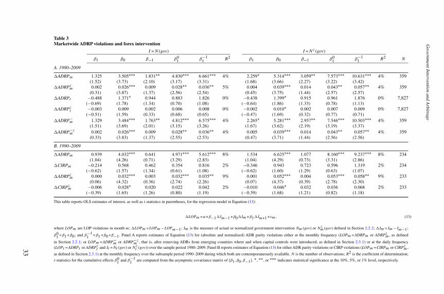
[14:5219/7/2017

RF

S-hhx074.tex]

Page:33

1–65

Governm

entInterventionand

Arbitrage

Table 3Marketwide ADRP violations and forex intervention

I =N (gov) I =Nz (gov)

β1 β0 β−1 β01 β−1

1 R2 β1 β0 β−1 β01 β−1

1 R2 N

A. 1980–2009

�ADRPm 1.325 3.505∗∗∗ 1.831∗∗ 4.830∗∗∗ 6.661∗∗∗ 4% 2.259∗ 5.314∗∗∗ 3.059∗∗ 7.573∗∗∗ 10.631∗∗∗ 4% 359(1.52) (3.73) (2.10) (3.17) (3.31) (1.68) (3.66) (2.27) (3.22) (3.42)

�ADRPzm 0.002 0.026∗∗∗ 0.009 0.028∗∗ 0.036∗∗ 5% 0.004 0.039∗∗∗ 0.014 0.043∗∗ 0.057∗∗ 4% 359(0.31) (3.87) (1.37) (2.56) (2.54) (0.45) (3.75) (1.44) (2.57) (2.57)

�ADRPt −0.488 1.371∗ 0.944 0.883 1.826 0% −0.438 1.399∗ 0.915 0.961 1.876 0% 7,827(−0.69) (1.78) (1.34) (0.70) (1.08) (−0.64) (1.86) (1.33) (0.78) (1.13)

�ADRPzt −0.003 0.009 0.002 0.006 0.008 0% −0.002 0.010∗ 0.002 0.007 0.009 0% 7,827(−0.51) (1.59) (0.33) (0.68) (0.65) (−0.47) (1.69) (0.32) (0.77) (0.71)

�ADRP−m 1.329 3.484∗∗∗ 1.763∗∗ 4.812∗∗∗ 6.575∗∗∗ 4% 2.265∗ 5.281∗∗∗ 2.957∗∗ 7.546∗∗∗ 10.503∗∗∗ 4% 359

(1.51) (3.69) (2.01) (3.15) (3.26) (1.67) (3.62) (2.19) (3.19) (3.37)�ADRP−z

m 0.002 0.026∗∗∗ 0.009 0.028∗∗ 0.036∗∗ 4% 0.005 0.039∗∗∗ 0.014 0.043∗∗ 0.057∗∗ 4% 359(0.33) (3.83) (1.37) (2.55) (2.53) (0.47) (3.71) (1.44) (2.56) (2.56)

B. 1990–2009

�ADRPm 0.939 4.032∗∗∗ 0.641 4.971∗∗∗ 5.612∗∗∗ 8% 1.534 6.625∗∗∗ 1.077 8.160∗∗∗ 9.237∗∗∗ 8% 234(1.04) (4.26) (0.71) (3.29) (2.83) (1.04) (4.29) (0.73) (3.31) (2.86)

�CIRPm −0.214 0.568 0.462 0.354 0.816 2% −0.346 0.943 0.723 0.596 1.319 2% 234(−0.62) (1.57) (1.34) (0.61) (1.08) (−0.62) (1.60) (1.29) (0.63) (1.07)

�ADRPzm 0.000 0.032∗∗∗ 0.003 0.032∗∗∗ 0.035∗∗ 9% 0.001 0.052∗∗∗ 0.004 0.053∗∗∗ 0.058∗∗ 9% 233(0.06) (4.32) (0.36) (2.74) (2.26) (0.07) (4.37) (0.39) (2.78) (2.30)

�CIRPzm −0.006 0.028∗ 0.020 0.022 0.042 2% −0.010 0.046∗ 0.032 0.036 0.068 2% 233(−0.39) (1.65) (1.26) (0.80) (1.19) (−0.39) (1.68) (1.21) (0.82) (1.18)

This table reports OLS estimates of interest, as well as t-statistics in parentheses, for the regression model in Equation (13):

�LOPm =α+β−1�Im−1 +β0�Im+β1�Im+1 +εm, (13)

where LOPm are LOP violations in month m; �LOPm =LOPm−LOPm−1; Im is the measure of actual or normalized government intervention Nm (gov) or Nzm (gov) defined in Section 2.2.2; �Im =Im−Im−1;

β01 =β1 +β0; and β−1

1 =β1 +β0 +β−1. Panel A reports estimates of Equation (13) for (absolute and normalized) ADR parity violations either at the monthly frequency (LOPm =ADRPm or ADRPzm , as defined

in Section 2.2.1; or LOPm =ADRP−m or ADRP−z

m , that is, after removing ADRs from emerging countries where and when capital controls were introduced, as defined in Section 2.3.1) or at the daily frequency(LOPt =ADRPt or ADRPzt and It =Nt (gov) orNzt (gov)) over the sample period 1980–2009. Panel B reports estimates of Equation (13) for either ADR parity violations or CIRP violations (LOPm =CIRPm or CIRPzm ,

as defined in Section 2.3.1) at the monthly frequency over the subsample period 1990–2009 during which both are contemporaneously available. N is the number of observations; R2 is the coefficient of determination;

t-statistics for the cumulative effects β01 and β−1

1 are computed from the asymptotic covariance matrix of {β1,β0,β−1}. ∗ , ∗∗ , or ∗∗∗ indicates statistical significance at the 10%, 5%, or 1% level, respectively.

33

[14:52 19/7/2017 RFS-hhx074.tex] Page: 34 1–65


deviation of�ADRPm. In unreported analysis, I find the estimation of Equation(13) to yield qualitatively similar inference within each decade of the sampleperiod.

2.3.1 Endogeneity bias. Coefficient estimates from the regression model ofEquation (13) may be plagued by possible endogeneity bias. As shown inEquation (11), violations of theADR parity (Pi,t �=P LOP

i,t ) may originate from theU.S. stock market where the ADR is traded (Pi,t ), the market for the underlyingforeign stock (P FOR

i,t ), and/or the market for the relevant exchange rate relativeto USD (St,USD/FOR). As discussed earlier, official trading activity in currencymarkets is unlikely to be motivated by the intensity of LOP violations inthe ADR market. Accordingly, while forex interventions occasionally may beanticipated by currency market participants, estimates of their lead effect β1

on ADRP violations in Equation (13) are always small and rarely significantin panel A of Table 3. Forex interventions are also most often sterilized, thatis, do not affect money supply or funding liquidity conditions; hence, theyare unlikely to be aimed at mitigating otherwise deteriorating (foreign and/orU.S.) stock market quality. However, forex interventions are likely to occur incorrespondence with, or in response to high exchange rate volatility (e.g., Neely2006) and tend to be accompanied by deteriorating currency market quality(e.g., Dominguez 2003, 2006; Pasquariello 2007b). Thus,ADRPviolations maybe large in months when currency market quality is low (e.g., Pasquariello 2008,2014)—which is exactly when governments are more likely to intervene—rather than as a consequence of forex interventions (e.g., Neely and Weller2007). Unfortunately, those properties of forex interventions also make itextremely difficult to find covariates of Im that are uncorrelated with the errorterm εt in Equation (13) to obtain consistent estimates of the impact coefficients(β1, β0, β−1) in Equation (13) via an instrumental variable (IV) approach (e.g.,Fatum and Hutchison 2003; Neely 2005, 2006; Engel 2014).

I assess the relevance of these considerations for the inference in variousways. First, I estimate Equation (13) for daily changes in actual or historicallyabnormal ADR parity violations (ADRPt or ADRPzt ) and the actual orhistorically abnormal number of forex interventions in a day (Nt (gov) orNzt (gov)). Omitted variable bias may be mitigated at higher, for example,

daily frequencies (see, e.g., Humpage and Osterberg 1992; Andersen et al.2003, 2007; and references therein). However, as discussed in Section 2.1,daily ADR parity violations are also significantly more volatile and morelikely to be spurious because of microstructure frictions (see also Gagnon andKarolyi 2010);35 forex interventions are often executed and coordinated over

35 For instance, the daily (monthly) sample standard deviation of ADRPt (ADRPm) is 92 bps (41 bps in Table 1),or 42% (21%) of its daily (monthly) sample mean. Gagnon and Karolyi (2010) address one such microstructurefriction—nonsynchronicity between foreign stock and ADR prices—by employing intraday price and quote datafor the latter (from TAQ) observed at the closing time of the equity market for the former, as long as their trading

34

[14:52 19/7/2017 RFS-hhx074.tex] Page: 35 1–65


several clustered days or even weeks, rather than on single, less salient eventdays; market participants may learn about such official trading activity, andits full effects on the targeted currency may manifest, only with considerabledelay (see, e.g., Neely 2000; Pasquariello 2007b). All are likely to weakenthe estimated relation between forex interventions and ADRP violations.Nonetheless, the resulting estimates of β1, β0, and β−1 in panel A of Table 3indicate that daily official trading activity in the currency market still has apositive and weakly significant (but unanticipated and short-lived) impact on�ADRPt and �ADRP zt , consistent with the model.

Second, I use Equation (13) to estimate the impact of forex interventions onviolations of the covered interest rate parity (CIRP). The CIRP is perhaps themost popular textbook no-arbitrage condition. According to the CIRP, in theabsence of arbitrage, spot and forward exchange rates between two currenciesand their nominal interest rates in international money markets should ensurethat riskless borrowing in one currency and lending in another, while hedgingcurrency risk, generates no riskless profit. The literature documents frequent,albeit generally small violations of the CIRP over the past three decadesand attributes their occurrence and magnitude to numerous observable andunobservable frictions to price formation in both currency and internationalmoney markets (see, e.g., Frenkel and Levich 1975, 1977; Coffey et al.2009; Griffoli and Ranaldo 2011; Pasquariello, Roush, and Vega 2014; andthe references therein). Since both markets have long been nearly perfectlyintegrated in many respects, including dealership (e.g., McKinnon (1977);Dufey and Giddy 1994; Bekaert and Hodrick 2012), my model predicts thatgovernment intervention in currency markets should have no impact on theextent of CIRP violations—that is,�corr (p1,1,p1,2)=0; see H1 in Section 1.3.However, the aforementioned literature also argues that greater CIRP violationsmay be due to deteriorating currency market quality—an omitted variable that,as I noted above, may be linked to forex intervention and so bias upward theestimates of its impact on ADR parity violations in Equation (13). Hence, thestrength of the relation between forex intervention and CIRP violations mayhint at the importance of this bias for those estimates.

To that purpose, I obtain the time series of actual and normalized monthlyCIRP violations, CIRPm and CIRPzm, constructed by Pasquariello, Roush, andVega (2014). Both measures of CIRP violations are monthly averages of actualand normalized daily absolute log differences (in bps, as in Equation (12)and Section 2.2.1) between daily indicative (short- and long-term maturity)forward exchange rates for five of the most actively traded and liquid currenciesin the forex market (CHF, EUR, GBP, USD, JPY; from Datastream) and the

hours are at least partially overlapping. However, this is not the case for Asian stock markets. In addition, TAQdata are available only from 1993 onward, while much forex intervention activity is concentrated in the 1980sand early 1990s (see, e.g., Figure 3A). Lastly, both the level and dynamics of ADRP violations in my sample areconsistent with what is reported in Gagnon and Karolyi (2010) over their sample period 1993-2004.

35

[14:52 19/7/2017 RFS-hhx074.tex] Page: 36 1–65


corresponding synthetic forward exchange rates implied by the CIRP. Becauseof data limitations, either series is exclusively available over a portion ofmy sample period, between either May (CIRPm) or June 1990 (CIRPzm)and December 2009. Pasquariello, Roush, and Vega (2014) reports that CIRPviolations within this subperiod are small, for example, averaging roughly 21bps (versus a concurrent mean ADRPm of 187 bps), but are also volatile andoften much larger in correspondence with well-known episodes of financialturmoil (like ADRP violations in Figure 3).36

I then estimate the regression model of Equation (13) over the subperiod1990-2009 for monthly changes in both ADRP (�LOPm=�ADRPm or�ADRP zm) and CIRP violations (�LOPm=�CIRPm or �CIRP zm). Theresulting estimated coefficients β1, β0, and β−1 in panel B of Table 3 suggestthat during that common interval of data availability, forex interventions havelittle or no impact on CIRP violations, that is, on LOP violations within the moreclosely integrated currency and international money markets. However, thoseinterventions continue to be accompanied by a large and persistent increase inADRP violations, that is, in LOP violations within the less closely integratedcurrency and ADR markets. This evidence not only provides further supportfor the model but also suggests that deteriorating currency market quality, asproxied by CIRP violations, is unlikely to be related to periods of intensifyingforex intervention and ADR parity violations.

Lastly, government interventions in emerging currency markets during timesof distress are occasionally accompanied by the imposition of capital controls(e.g., East Asia in the 1990s; Argentina in 2001–2002; Brazil in 2008–2009),which may impede ADR arbitrage activity by restricting foreign ownershipof local shares or local ownership of foreign shares as well as by introducinguncertainty about either (see Edison and Warnock 2003; Auguste et al. 2006;Gagnon and Karolyi 2010; Garleanu and Pedersen 2011). Nonetheless, panel Aof Table 3 shows that the exclusion of cross-listings from so-affected countriesin the sample from both measures of marketwide ADRP violations over theportion of the sample period when these restrictions were in place (ADRP−

m

and ADRP−zm ) has no effect on the inference from Equation (13).

2.4 The cross-section of ADRP violationsAccording to Table 3, there is a positive and economically and statisticallysignificant relation between changes in ADR parity violations and changes inthe intensity of forex intervention, as postulated in Conclusion 1.

I also postulate in Conclusion 2 that the impact of government interventionin one asset on LOP violations—that is, on the equilibrium correlation betweenits price and the price of another, otherwise identical or arbitrage-linked asset(corr

(p∗

1,1,p∗1,2

)of Equation (10))—may depend on such variables affecting the

36 For further details on the construction of these series and their properties, see Pasquariello (2014; Section 1.1.1).

36

[14:52 19/7/2017 RFS-hhx074.tex] Page: 37 1–65


underlying quality of the markets in which those assets are traded as the intensityand correlation of noise trading, or the extent of and adverse selection riskfrom informed, strategic speculation. These variables, although intrinsicallyconceptual and difficult to measure for each ADR or within each ADR market,may be plausibly related to such observable market characteristics as eachADR’s country of listing (e.g., Gagnon and Karolyi 2010), as well as to suchobservable ADR market quality outcomes as each ADR’s illiquidity and no-arbitrage parity violations (e.g., Pasquariello 2008, 2014). Investigating thecross-section of the impact of forex intervention on ADRP violations alongthose dimensions may shed further light on its theoretical determinants, andthus further alleviate the aforementioned endogeneity concerns plaguing theinference from Table 3.

To this end, I estimate the regression model of Equation (13) separatelyfor each country of listing in Table 1, for each of the five countries forwhich currency-matched intervention-ADR pairs are available within thesample (Australia, Euro area, Japan, Mexico, and Turkey; see Table 2 andSection 2.2.2), as well as for each tercile portfolio of cross-listings sorted byeither their sample mean ADRP illiquidity ILLIQm or their sample mean actualabsolute ADRP violations ADRPm (as defined in Section 2.2.1, from the lowestto the highest), when correspondingly available.37 I then report the resultingcoefficients of interest for either actual or normalized absoluteADRP violations(LOPm=ADRPm or ADRPzm) in panels A and B of Tables 4 to 7, respectively.Noisier but qualitatively similar inference ensues from (unreported) cross-sectional estimates of Equation (13) at the daily frequency (LOPt =ADRPtor ADRPzt ) and/or for quintile sorts.

My model suggests that estimates of the positive relation between forexintervention and ADR parity violations may be complexly linked to underlyingADR market quality. For instance, as noted in Section 1.2, governmentintervention may yield larger LOP violations (larger �corr (p1,1,p1,2))when the underlying, arbitrage-linked markets are less liquid (higher λand λ∗)—indicating low underlying market quality; for example, for lessintense noise trading (see Figure 1D; H3 in Section 1.3). However,�corr (p1,1,p1,2) may also be larger when underlying LOP violations areeither smaller (larger corr (p1,1,p1,2))—indicating high market quality; forexample, for more correlated noise trading (Figure 1A)—or larger (smallercorr (p1,1,p1,2))—indicating low market quality; for example, for fewer and/ormore heterogeneously informed speculators (Figures 1B and 1C). On theother hand, �corr (p1,1,p1,2) may be smaller not only when corr (p1,1,p1,2)is smaller—indicating low market quality; for example, for less correlatednoise trading—but also when it is larger—indicating high market quality; for

37 Despite uneven sample coverage across usable ADRs (see, e.g., Table 1), actual and normalized LOP violationdata for each of the ensuing sorts are always available over the sample period 1980-2009, with the exception ofthe high-ADRPm tercile, which is only populated since either November (ADRPm) or December 1985 (ADRPzm).

37

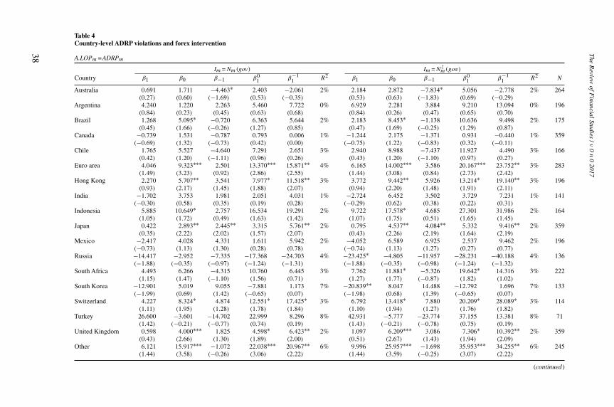
[14:5219/7/2017

RF

S-hhx074.tex]

Page:38

1–65

The

Review

ofFinancialStudies

/v0

n0

2017

Table 4Country-level ADRP violations and forex intervention

A.LOPm =ADRPm

Im =Nm (gov) Im =Nzm (gov)

Country β1 β0 β−1 β01 β−1

1 R2 β1 β0 β−1 β01 β−1

1 R2 N

Australia 0.691 1.711 −4.463∗ 2.403 −2.061 2% 2.184 2.872 −7.834∗ 5.056 −2.778 2% 264(0.27) (0.60) (−1.69) (0.53) (−0.35) (0.53) (0.63) (−1.83) (0.69) (−0.29)

Argentina 4.240 1.220 2.263 5.460 7.722 0% 6.929 2.281 3.884 9.210 13.094 0% 196(0.84) (0.23) (0.45) (0.63) (0.68) (0.84) (0.26) (0.47) (0.65) (0.70)

Brazil 1.268 5.095∗ −0.720 6.363 5.644 2% 2.183 8.453∗ −1.138 10.636 9.498 2% 175(0.45) (1.66) (−0.26) (1.27) (0.85) (0.47) (1.69) (−0.25) (1.29) (0.87)

Canada −0.739 1.531 −0.787 0.793 0.006 1% −1.244 2.175 −1.371 0.931 −0.440 1% 359(−0.69) (1.32) (−0.73) (0.42) (0.00) (−0.75) (1.22) (−0.83) (0.32) (−0.11)

Chile 1.765 5.527 −4.640 7.291 2.651 3% 2.940 8.988 −7.437 11.927 4.490 3% 166(0.42) (1.20) (−1.11) (0.96) (0.26) (0.43) (1.20) (−1.10) (0.97) (0.27)

Euro area 4.046 9.323∗∗∗ 2.501 13.370∗∗∗ 15.871∗∗ 4% 6.165 14.002∗∗∗ 3.586 20.167∗∗∗ 23.752∗∗ 3% 283(1.49) (3.23) (0.92) (2.86) (2.55) (1.44) (3.08) (0.84) (2.73) (2.42)

Hong Kong 2.270 5.707∗∗ 3.541 7.977∗ 11.518∗∗ 3% 3.772 9.442∗∗ 5.926 13.214∗ 19.140∗∗ 3% 196(0.93) (2.17) (1.45) (1.88) (2.07) (0.94) (2.20) (1.48) (1.91) (2.11)

India −1.702 3.753 1.981 2.051 4.031 1% −2.724 6.452 3.502 3.729 7.231 1% 141(−0.30) (0.58) (0.35) (0.19) (0.28) (−0.29) (0.62) (0.38) (0.22) (0.31)

Indonesia 5.885 10.649∗ 2.757 16.534 19.291 2% 9.722 17.578∗ 4.685 27.301 31.986 2% 164(1.05) (1.72) (0.49) (1.63) (1.42) (1.07) (1.75) (0.51) (1.65) (1.45)

Japan 0.422 2.893∗∗ 2.445∗∗ 3.315 5.761∗∗ 2% 0.795 4.537∗∗ 4.084∗∗ 5.332 9.416∗∗ 2% 359(0.35) (2.22) (2.02) (1.57) (2.07) (0.43) (2.26) (2.19) (1.64) (2.19)

Mexico −2.417 4.028 4.331 1.611 5.942 2% −4.052 6.589 6.925 2.537 9.462 2% 196(−0.73) (1.13) (1.30) (0.28) (0.78) (−0.74) (1.13) (1.27) (0.27) (0.77)

Russia −14.417 −2.952 −7.335 −17.368 −24.703 4% −23.425∗ −4.805 −11.957 −28.231 −40.188 4% 136(−1.88) (−0.35) (−0.97) (−1.24) (−1.31) (−1.88) (−0.35) (−0.98) (−1.24) (−1.32)

South Africa 4.493 6.266 −4.315 10.760 6.445 3% 7.762 11.881∗ −5.326 19.642∗ 14.316 3% 222(1.15) (1.47) (−1.10) (1.56) (0.71) (1.27) (1.77) (−0.87) (1.82) (1.02)

South Korea −12.901 5.019 9.055 −7.881 1.173 7% −20.839∗∗ 8.047 14.488 −12.792 1.696 7% 133(−1.99) (0.69) (1.42) (−0.65) (0.07) (−1.98) (0.68) (1.39) (−0.65) (0.07)

Switzerland 4.227 8.324∗ 4.874 12.551∗ 17.425∗ 3% 6.792 13.418∗ 7.880 20.209∗ 28.089∗ 3% 114(1.11) (1.95) (1.28) (1.78) (1.84) (1.10) (1.94) (1.27) (1.76) (1.82)

Turkey 26.600 −3.601 −14.702 22.999 8.296 8% 42.931 −5.777 −23.774 37.155 13.381 8% 71(1.42) (−0.21) (−0.77) (0.74) (0.19) (1.43) (−0.21) (−0.78) (0.75) (0.19)

United Kingdom 0.598 4.000∗∗∗ 1.825 4.598∗ 6.423∗∗ 2% 1.097 6.209∗∗∗ 3.086 7.306∗ 10.392∗∗ 2% 359(0.43) (2.66) (1.30) (1.89) (2.00) (0.51) (2.67) (1.43) (1.94) (2.09)

Other 6.121 15.917∗∗∗ −1.072 22.038∗∗∗ 20.967∗∗ 6% 9.996 25.957∗∗∗ −1.698 35.953∗∗∗ 34.255∗∗ 6% 245(1.44) (3.58) (−0.26) (3.06) (2.22) (1.44) (3.59) (−0.25) (3.07) (2.22)

(continued )

38

[14:5219/7/2017

RF

S-hhx074.tex]

Page:39

1–65

Governm

entInterventionand

Arbitrage

Table 4Continued

B. LOPm =ADRPzm


Country β1 β0 β−1 β01 β

−11 R2 β1 β0 β−1 β0

1 β−11 R2 N

Australia −0.009 0.021 −0.005 0.012 0.007 2% −0.012 0.035 −0.007 0.023 0.016 2% 259(−0.64) (1.42) (−0.37) (0.52) (0.23) (−0.54) (1.45) (−0.32) (0.61) (0.32)

Argentina 0.050 0.022 0.020 0.072 0.092 1% 0.081 0.039 0.035 0.120 0.155 1% 195(0.95) (0.40) (0.39) (0.80) (0.78) (0.95) (0.42) (0.41) (0.82) (0.80)

Brazil 0.003 0.044∗ −0.001 0.047 0.045 3% 0.006 0.074∗ −0.002 0.080 0.078 3% 173(0.11) (1.84) (−0.07) (1.17) (0.86) (0.15) (1.89) (−0.05) (1.22) (0.91)

Canada 0.000 0.012 −0.009 0.013 0.004 2% 0.001 0.017 −0.015 0.018 0.004 2% 359(0.03) (1.49) (−1.13) (0.94) (0.22) (0.09) (1.33) (−1.22) (0.87) (0.13)

Chile 0.004 0.021 −0.042 0.025 −0.016 3% 0.008 0.035 −0.067 0.042 −0.024 3% 165(0.16) (0.68) (−1.50) (0.50) (−0.24) (0.17) (0.70) (−1.48) (0.52) (−0.22)

Euro area 0.008 0.036∗ 0.003 0.044 0.047 1% 0.015 0.055∗ 0.002 0.069 0.071 1% 280(0.43) (1.78) (0.14) (1.35) (1.08) (0.49) (1.71) (0.06) (1.34) (1.03)

Hong Kong 0.008 0.054∗∗∗ 0.016 0.062∗∗ 0.078∗∗ 5% 0.013 0.089∗∗∗ 0.027 0.102∗∗ 0.130∗∗ 5% 195(0.46) (2.96) (0.95) (2.10) (2.01) (0.47) (2.99) (0.98) (2.12) (2.05)

India −0.021 0.062∗ 0.023 0.041 0.064 5% −0.034 0.102∗ 0.038 0.067 0.105 5% 140(−0.69) (1.80) (0.74) (0.71) (0.83) (−0.69) (1.80) (0.75) (0.72) (0.84)

Indonesia 0.036 0.060 0.012 0.096 0.108 2% 0.059 0.099 0.021 0.158 0.179 2% 163(1.06) (1.61) (0.36) (1.56) (1.32) (1.08) (1.64) (0.39) (1.59) (1.35)

Japan −0.004 0.023∗ 0.024∗∗ 0.019 0.044 2% −0.005 0.036∗ 0.040∗∗ 0.030 0.070∗ 2% 359(−0.32) (1.81) (2.05) (0.93) (1.60) (−0.29) (1.81) (2.18) (0.95) (1.67)

Mexico −0.021 0.031∗ 0.014 0.011 0.024 3% −0.034 0.052∗ 0.022 0.017 0.039 4% 195(−1.18) (1.69) (0.78) (0.36) (0.62) (−1.20) (1.70) (0.77) (0.35) (0.61)

Russia −0.034 0.001 −0.030 −0.032 −0.062 2% −0.054 0.003 −0.048 −0.051 −0.099 2% 135(−0.94) (0.03) (−0.84) (−0.49) (−0.70) (−0.92) (0.04) (−0.85) (−0.47) (−0.69)

South Africa 0.014 0.038∗∗ 0.001 0.052∗ 0.052 2% 0.026 0.066∗∗ 0.006 0.092∗ 0.098 2% 222(0.81) (1.97) (0.03) (1.68) (1.30) (0.93) (2.22) (0.20) (1.91) (1.55)

South Korea −0.030 0.014 0.017 −0.016 0.001 3% −0.048 0.023 0.028 −0.025 0.003 3% 132(−1.18) (0.49) (0.69) (−0.34) (0.02) (−1.16) (0.50) (0.68) (−0.33) (0.03)

Switzerland 0.032 0.078∗∗∗ 0.058∗∗ 0.110∗∗ 0.168∗∗ 7% 0.053 0.128∗∗∗ 0.095∗∗ 0.181∗∗ 0.276∗∗ 7% 113(1.23) (2.65) (2.20) (2.27) (2.57) (1.25) (2.68) (2.22) (2.29) (2.60)

Turkey 0.152 −0.055 −0.098 0.096 −0.001 9% 0.245 −0.089 −0.158 0.156 −0.002 9% 70(1.35) (−0.53) (−0.86) (0.52) (−0.01) (1.36) (−0.53) (−0.87) (0.52) (−0.00)

United Kingdom −0.003 0.023∗∗ 0.002 0.020 0.022 2% −0.003 0.034∗∗ 0.003 0.031 0.034 2% 359(−0.29) (2.43) (0.24) (1.33) (1.11) (−0.23) (2.34) (0.22) (1.31) (1.09)

Other 0.022 0.085∗∗∗ 0.001 0.107∗∗∗ 0.108∗∗∗ 9% 0.036 0.138∗∗∗ 0.002 0.174∗∗∗ 0.176∗∗∗ 9% 244(1.22) (4.43) (0.04) (3.45) (2.65) (1.22) (4.43) (0.06) (3.45) (2.65)



where LOPm are LOP violations in monthm;�LOPm =LOPm−LOPm−1; Im is the measure of actual or normalized government interventionNm (gov) orNzm (gov) defined in Section 2.2.2;

�Im =Im−Im−1; β01 =β1 +β0; and β−1

1 =β1 +β0 +β−1. Specifically, Equation (13) is estimated separately, at the monthly frequency, for each of the 18 countries listed in Table 1 (Australia,Argentina, Brazil, Canada, Chile, Euro area, Hong Kong, India, Indonesia, Japan, Mexico, Russia, South Africa, South Korea, Switzerland, Turkey, United Kingdom, and Other) overthe portion of the sample period 1980–2009 over which ADRP violation data are correspondingly available. In panel A, LOPm =ADRPm (absolute ADRP violations); in panel B,LOPm =ADRPzm (normalized ADRP violations), as defined in Section 2.2.1. N is the number of observations; R2 is the coefficient of determination; t-statistics for the cumulativeeffects β0

1 and β−11 are computed from the asymptotic covariance matrix of {β1, β0, β−1}. ∗, ∗∗, or ∗∗∗ indicates statistical significance at the 10%, 5%, or 1% level, respectively.

39

[14:52 19/7/2017 RFS-hhx074.tex] Page: 40 1–65


example, for more numerous and/or less heterogeneously informed speculators.See also the plots of �corr (p1,1,p1,2) versus λ and corr (p1,1,p1,2) inFigures 2B and 2C, respectively.

Accordingly, country-level estimates of the contemporaneous (β0) andcumulative impact (β0

1 and β−11 ) of changes in either Nm (gov) or Nz

m (gov)on absolute percentage ADR parity violations in Table 4 tend to be more oftenpositive, large, and/or significant for cross-listings from emerging markets,which typically have a lower quality information environment (e.g., Bekaertand Harvey 1995, 1997, 2000, 2003; Lesmond 2005; Pasquariello 2008), aswell as for cross-listings whose samplewide mean ADRP violations (ADRPm)and/or illiquidity (ILLIQm) in Table 1 tend to be either high (like in Figure 2C[solid line] and H3) or low (like in Figure 2C [dashed line], yet unlike H3). Forinstance, panel A of Table 4 shows that, on average, a one-standard-deviationincrease in �Nz

m (gov) is accompanied by a large cumulative increase in LOPviolations for cross-listings both from markets with high mean ADRPm and/orILLIQm—for example, South Africa (13 bps, i.e., 20% of the correspondingstandard deviation of �ADRPm in Table 1), Hong Kong (13 bps, 44%), andOther (mostly emerging countries, listed in Table 1; 31 bps, 37%)—as well asfrom markets with low mean ADRPm and/or ILLIQm—for example, Japan (9bps, 29%), Euro area (22 bps, 35%), and Switzerland (26 bps, 69%).38

While generally consistent with the model’s predictions, the evidence inTable 4 is only suggestive. Especially emerging country-level groupings consistof fewer usable ADRs over shorter periods (see Table 1), such that boththeir measures of ADRP violations and their estimated relation with forexintervention are noisier. Country-level sorting may also subsume additional,albeit possibly nonexclusive interpretations. For instance, greater or lowerilliquidity in emerging markets may be both unrelated to adverse selectionrisk and still associated with more limited arbitrage activity in the presenceof government-induced LOP violations. Estimates of the impact of currency-matched intervention on ADRP violations in Table 5 yield similar insight, asthey are mostly positive (except for Turkey, as in Table 4) and generally large,but are statistically significant only Australia, the Euro area, and (to a lesserextent) Mexico, which have a relatively large number of interventions (seeTables 1 and 2).

Further estimation of Equation (13) for illiquidity-sorted and LOP violation-sorted ADRP portfolios in Tables 6 and 7 confirms that the observed relationbetween the negative arbitrage externality of forex intervention and ADRs’underlying market quality may be rather complex—broadly, albeit weakly andonce again only suggestively consistent with the model. For instance, estimates

38 The Hong Kong dollar (HKD) has been pegged against USD at different levels over my sample period. SinceNm (gov) and Nzm (gov) measure the intensity of government intervention in the forex market, the evidence inTable 4 is consistent with the notion that ADR prices, Pi,t , may reflect ensuing expectations that a peg forSFOR/USD,t may be altered or abandoned in the future (e.g., Auguste et al. 2006; Eichler, Karmann, andMaltritz 2009).

40

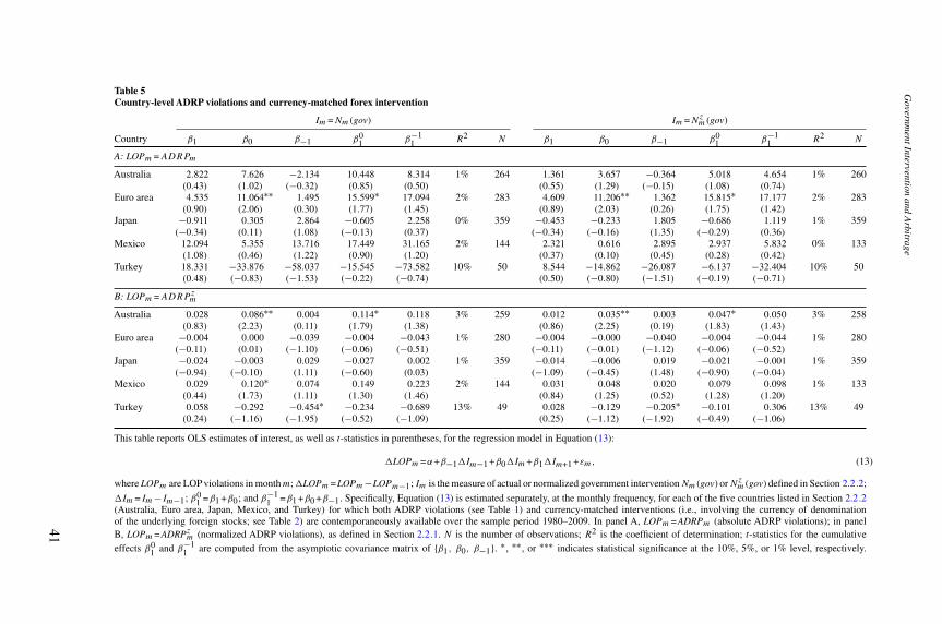
[14:5219/7/2017

RF

S-hhx074.tex]

Page:41

1–65

Governm

entInterventionand

Arbitrage

Table 5Country-level ADRP violations and currency-matched forex intervention


Country β1 β0 β−1 β01 β−1

1 R2 N β1 β0 β−1 β01 β−1

1 R2 N

A: LOPm =ADRPm

Australia 2.822 7.626 −2.134 10.448 8.314 1% 264 1.361 3.657 −0.364 5.018 4.654 1% 260(0.43) (1.02) (−0.32) (0.85) (0.50) (0.55) (1.29) (−0.15) (1.08) (0.74)

Euro area 4.535 11.064∗∗ 1.495 15.599∗ 17.094 2% 283 4.609 11.206∗∗ 1.362 15.815∗ 17.177 2% 283(0.90) (2.06) (0.30) (1.77) (1.45) (0.89) (2.03) (0.26) (1.75) (1.42)

Japan −0.911 0.305 2.864 −0.605 2.258 0% 359 −0.453 −0.233 1.805 −0.686 1.119 1% 359(−0.34) (0.11) (1.08) (−0.13) (0.37) (−0.34) (−0.16) (1.35) (−0.29) (0.36)

Mexico 12.094 5.355 13.716 17.449 31.165 2% 144 2.321 0.616 2.895 2.937 5.832 0% 133(1.08) (0.46) (1.22) (0.90) (1.20) (0.37) (0.10) (0.45) (0.28) (0.42)

Turkey 18.331 −33.876 −58.037 −15.545 −73.582 10% 50 8.544 −14.862 −26.087 −6.137 −32.404 10% 50(0.48) (−0.83) (−1.53) (−0.22) (−0.74) (0.50) (−0.80) (−1.51) (−0.19) (−0.71)

B: LOPm =ADRPzm

Australia 0.028 0.086∗∗ 0.004 0.114∗ 0.118 3% 259 0.012 0.035∗∗ 0.003 0.047∗ 0.050 3% 258(0.83) (2.23) (0.11) (1.79) (1.38) (0.86) (2.25) (0.19) (1.83) (1.43)

Euro area −0.004 0.000 −0.039 −0.004 −0.043 1% 280 −0.004 −0.000 −0.040 −0.004 −0.044 1% 280(−0.11) (0.01) (−1.10) (−0.06) (−0.51) (−0.11) (−0.01) (−1.12) (−0.06) (−0.52)

Japan −0.024 −0.003 0.029 −0.027 0.002 1% 359 −0.014 −0.006 0.019 −0.021 −0.001 1% 359(−0.94) (−0.10) (1.11) (−0.60) (0.03) (−1.09) (−0.45) (1.48) (−0.90) (−0.04)

Mexico 0.029 0.120∗ 0.074 0.149 0.223 2% 144 0.031 0.048 0.020 0.079 0.098 1% 133(0.44) (1.73) (1.11) (1.30) (1.46) (0.84) (1.25) (0.52) (1.28) (1.20)

Turkey 0.058 −0.292 −0.454∗ −0.234 −0.689 13% 49 0.028 −0.129 −0.205∗ −0.101 0.306 13% 49(0.24) (−1.16) (−1.95) (−0.52) (−1.09) (0.25) (−1.12) (−1.92) (−0.49) (−1.06)




�Im =Im−Im−1; β01 =β1 +β0; and β−1

1 =β1 +β0 +β−1. Specifically, Equation (13) is estimated separately, at the monthly frequency, for each of the five countries listed in Section 2.2.2(Australia, Euro area, Japan, Mexico, and Turkey) for which both ADRP violations (see Table 1) and currency-matched interventions (i.e., involving the currency of denominationof the underlying foreign stocks; see Table 2) are contemporaneously available over the sample period 1980–2009. In panel A, LOPm =ADRPm (absolute ADRP violations); in panelB, LOPm =ADRPzm (normalized ADRP violations), as defined in Section 2.2.1. N is the number of observations; R2 is the coefficient of determination; t-statistics for the cumulativeeffects β0


41

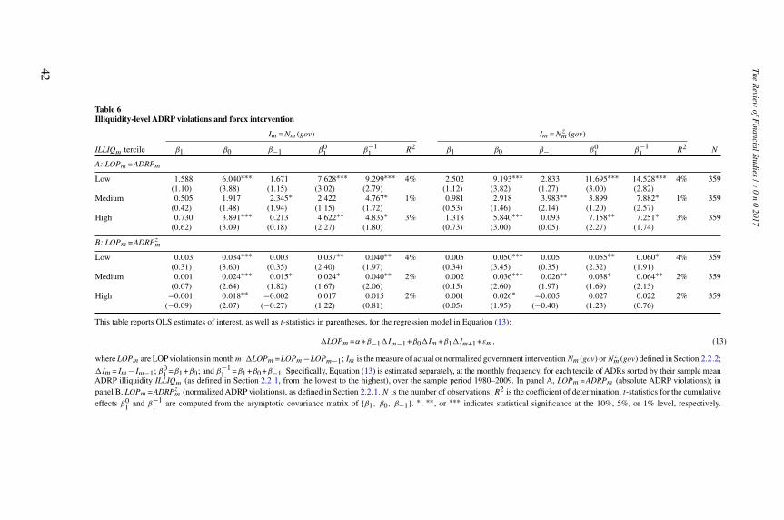
[14:5219/7/2017

RF

S-hhx074.tex]

Page:42

1–65

The

Review

ofFinancialStudies

/v0

n0

2017

Table 6Illiquidity-level ADRP violations and forex intervention


ILLIQm tercile β1 β0 β−1 β01 β−1

1 R2 β1 β0 β−1 β01 β−1

1 R2 N

A: LOPm =ADRPm

Low 1.588 6.040∗∗∗ 1.671 7.628∗∗∗ 9.299∗∗∗ 4% 2.502 9.193∗∗∗ 2.833 11.695∗∗∗ 14.528∗∗∗ 4% 359(1.10) (3.88) (1.15) (3.02) (2.79) (1.12) (3.82) (1.27) (3.00) (2.82)

Medium 0.505 1.917 2.345∗ 2.422 4.767∗ 1% 0.981 2.918 3.983∗∗ 3.899 7.882∗ 1% 359(0.42) (1.48) (1.94) (1.15) (1.72) (0.53) (1.46) (2.14) (1.20) (2.57)

High 0.730 3.891∗∗∗ 0.213 4.622∗∗ 4.835∗ 3% 1.318 5.840∗∗∗ 0.093 7.158∗∗ 7.251∗ 3% 359(0.62) (3.09) (0.18) (2.27) (1.80) (0.73) (3.00) (0.05) (2.27) (1.74)

B: LOPm =ADRPzm

Low 0.003 0.034∗∗∗ 0.003 0.037∗∗ 0.040∗∗ 4% 0.005 0.050∗∗∗ 0.005 0.055∗∗ 0.060∗ 4% 359(0.31) (3.60) (0.35) (2.40) (1.97) (0.34) (3.45) (0.35) (2.32) (1.91)

Medium 0.001 0.024∗∗∗ 0.015∗ 0.024∗ 0.040∗∗ 2% 0.002 0.036∗∗∗ 0.026∗∗ 0.038∗ 0.064∗∗ 2% 359(0.07) (2.64) (1.82) (1.67) (2.06) (0.15) (2.60) (1.97) (1.69) (2.13)

High −0.001 0.018∗∗ −0.002 0.017 0.015 2% 0.001 0.026∗ −0.005 0.027 0.022 2% 359(−0.09) (2.07) (−0.27) (1.22) (0.81) (0.05) (1.95) (−0.40) (1.23) (0.76)




�Im =Im−Im−1; β01 =β1 +β0; and β−1

1 =β1 +β0 +β−1. Specifically, Equation (13) is estimated separately, at the monthly frequency, for each tercile of ADRs sorted by their sample meanADRP illiquidity ILLIQm (as defined in Section 2.2.1, from the lowest to the highest), over the sample period 1980–2009. In panel A, LOPm =ADRPm (absolute ADRP violations); inpanel B, LOPm =ADRPzm (normalized ADRP violations), as defined in Section 2.2.1. N is the number of observations; R2 is the coefficient of determination; t-statistics for the cumulativeeffects β0


42

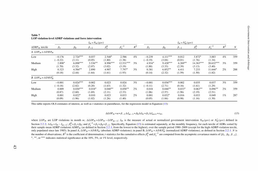
[14:5219/7/2017

RF

S-hhx074.tex]

Page:43

1–65

Governm

entInterventionand

Arbitrage

Table 7LOP violation-level ADRP violations and forex intervention


ADRPm tercile β1 β0 β−1 β01 β−1

1 R2 β1 β0 β−1 β01 β−1

1 R2 N

A. LOPm =ADRPm

Low −0.176 2.724∗∗∗ 0.037 2.548∗ 2.586 4% −0.239 4.111∗∗∗ 0.012 3.872∗ 3.883 4% 359(−0.22) (3.11) (0.05) (1.80) (1.38) (−0.19) (3.04) (0.01) (1.76) (1.34)

Medium 2.898∗ 6.098∗∗∗ 3.536∗∗ 8.996∗∗∗ 12.531∗∗∗ 3% 4.934∗ 9.428∗∗∗ 6.269∗∗ 14.363∗∗∗ 20.632∗∗∗ 3% 359(1.70) (3.32) (2.07) (3.02) (3.19) (1.88) (3.33) (2.39) (3.13) (3.40)

High 0.323 4.584∗∗ 2.890 4.907 7.797∗ 3% 0.381 6.852∗∗ 4.411 7.233 11.644∗ 2% 288(0.18) (2.44) (1.64) (1.61) (1.93) (0.14) (2.32) (1.59) (1.50) (1.82)

B. LOPm =ADRPzm

Low −0.001 0.024∗∗∗ 0.002 0.023 0.024 3% −0.001 0.036∗∗∗ 0.002 0.035 0.037 3% 359(−0.18) (2.82) (0.20) (1.63) (1.32) (−0.11) (2.71) (0.16) (1.61) (1.29)

Medium 0.009 0.030∗∗∗ 0.018∗ 0.040∗∗ 0.058∗∗ 2% 0.018 0.046∗∗ 0.033∗ 0.063∗∗ 0.096∗∗ 2% 359(0.87) (2.60) (1.69) (2.11) (2.33) (1.06) (2.57) (1.96) (2.19) (2.51)

High 0.001 0.022∗ 0.010 0.023 0.033 2% 0.001 0.032∗ 0.016 0.033 0.049 1% 287(0.09) (1.96) (1.02) (1.26) (1.40) (0.05) (1.84) (0.98) (1.16) (1.30)



where LOPm are LOP violations in month m; �LOPm =LOPm−LOPm−1; Im is the measure of actual or normalized government intervention Nm (gov) or Nzm (gov) defined in

Section 2.2.2; �Im =Im−Im−1; β01 =β1 +β0; and β−1

1 =β1 +β0 +β−1. Specifically, Equation (13) is estimated separately, at the monthly frequency, for each tercile of ADRs sorted bytheir sample mean ADRP violations ADRPm (as defined in Section 2.2.1, from the lowest to the highest), over the sample period 1980–2009 (except for the high-ADRP-violation tercile,only populated since late 1985). In panel A, LOPm =ADRPm (absolute ADRP violations); in panel B, LOPm =ADRPzm (normalized ADRP violations), as defined in Section 2.2.1. N isthe number of observations; R2 is the coefficient of determination; t-statistics for the cumulative effects β0

1 and β−11 are computed from the asymptotic covariance matrix of {β1, β0, β−1}.

∗, ∗∗, or ∗∗∗ indicates statistical significance at the 10%, 5%, or 1% level, respectively.

43

[14:52 19/7/2017 RFS-hhx074.tex] Page: 44 1–65


of the positive, contemporaneous and cumulative impact of forex interventionon ADRP violations are nonmonotonic, instead of increasing (e.g., Figure 2B;H3), in unconditional ADRP illiquidity ILLIQm (e.g., panel A of Table 6),perhaps because of the concurrent effect of other frictions and forces impedingboth liquidity provision and arbitrage activity in the ADR market. However,these estimates are also nonmonotonic in unconditional ADR parity violationsADRPm (e.g., panel B of Table 7), as hinted by the discussion in Section 1.2(e.g., Figure 2C), and up to twice as large for higher underlying market quality(e.g., low or medium ILLIQm or ADRPm) as for lower underlying market quality(high ILLIQm or ADRPm).

2.5 ADRP violations and market conditionsTables 3 to 7 indicate that government intervention in currency markets isaccompanied by a large and statistically significant increase in LOPviolations inADR markets. This evidence is consistent with the main empirical implicationof my model (H2 in Section 1.3). Yet, as noted earlier, this interpretationmay be clouded by the possible endogeneity of forex interventions and ADRPviolations, a concern that the additional time-series and cross-sectional analysisin Sections 2.3.1 and 2.4 can only mitigate. For instance, directly linkingthe cross-sectional tests in Tables 4 to 7 to the model of Section 1 may beproblematic since their conditioning variables (country of home listing, ADRPilliquidity, or ADRP violations) are plausibly related to alternative frictionsand theories as well. Unfortunately, most primitive parameters in the model—like the intensity and correlation of noise trading (σ 2

z and σzz) or the numberof multiasset speculators (M)—are directly unobservable (like in all modelsbased on Kyle 1985), their indirect estimation involves significant risk ofmeasurement error, and the relevant data is typically unavailable for mostcurrency and/or foreign stock markets (e.g., Allen and Taylor 1990; Madhavan2000; Caballé and Krishnan 2004; Lesmond 2005; Cong, Hoitash, and Krishnan2010).

In addition, the above evidence may also be consistent with another, albeitpossibly complementary interpretation related to trading risk—that is, one thatdoes not play a role in my model, where all market participants are risk-neutral.Forex intervention, rather than only constituting a source of LOP violations inthe ADR market given existing limits to arbitrage (as implied by the model;see Section 1.1), may itself also impede arbitrage activity, for instance, byintroducing a new source of unhedgeable convergence risk, in the spirit ofPontiff (1996), 2006), for speculators and arbitrageurs exploiting extant ADRPviolations. However, these market participants are also more likely to be ableto manage such a risk, and its severity is more likely to be attenuated—thus,their trading activity in the ADR market is less likely to be affected—at thelow, monthly frequency of my analysis.

In this section, I assess these notions more directly, by explicitly testing foradditional, unique predictions of the model, hence more difficult to reconcile

44

[14:52 19/7/2017 RFS-hhx074.tex] Page: 45 1–65


with endogeneity or alternative interpretations—such as those relating thenegative arbitrage externalities of government intervention to plausiblymeasurable market conditions affecting asset liquidity or policy uncertainty(H3 to H5)—as well as explicitly controlling for plausibly measurable statevariables that may affect the time-varying intensity of limits to arbitrageand/or of forex intervention activity. To that purpose, I amend the regressionmodel of Equation (13) for monthly changes in LOP violations (�LOPm) asfollows:

�LOPm=α+β0�Im+βILQ�ILLIQm+β2ILQ (�ILLIQm)2

+β ILQ0 �Im�ILLIQm+βDSP�DISPm+βDSP

0 �Im�DISPm (14)

+βSDI�STD(Im)+βSDI0 �Im�STD(Im)+��Xm+εm,

where LOPm is either ADRPm or ADRPzm, and Im is eitherNm (gov) orNzm (gov).

The inference is insensitive to introducing lead-lag effects of forex interventionand calendar fixed effects (or time trends), as well as robust to numerousplausible extensions and alternative specifications, some of which are notedbelow. Equation (14) allows for changes in ADRP illiquidity (�ILLIQm),marketwide information heterogeneity (�DISPm), and policy uncertainty(�STD(Im)) to affect the extent of LOP violations in the ADR market bothdirectly and through their interaction with forex intervention, as postulated bymy model.

As discussed in Section 2.2.1, ILLIQm, the equal weighted average of themarketwide fraction of zero returns in the arbitrage-linked ADR, foreign stock,and currency markets (Figure 4A), is designed to capture marketwide ADRparity-level illiquidity. The model predicts that either βILQ>0 or βILQ<0(Corollary 2), but β ILQ

0 >0 (Conclusion 2; H3), i.e., that ADRP violationsmay depend on, but their positive sensitivity to forex intervention (β0>

0) is likely greater in correspondence with, deteriorating ADRP liquidity(�ILLIQm>0). Intuitively, ceteris paribus, when markets are less deep inequilibrium (higher λ and λ∗; e.g., when there are fewer speculators, seeFigure 1C), noise trading shocks and government intervention in the aggregateorder flow have a greater impact on equilibrium prices, yielding larger LOPviolations (lower corr (p1,1,p1,2), e.g., Figure 2A [solid line]; and greater�corr (p1,1,p1,2), e.g., Figure 2B). However, as noted in Section 1.1.2, theobserved relation between �LOPm and �ILLIQm may also be negative, orpossibly nonmonotonic. For instance, according to Corollary 2, LOP violationsmay also be greater in the presence of more intense noise trading, despiteits lower price impact (lower λ and λ∗, see Figure 1D and Figure 2A[dashed line]). Thus, Equation (14) includes a quadratic term for �ILLIQm

as well.Among the determinants of market liquidity in the model, speculators’

information heterogeneity (ρ) plays an important role as it affects their

45

[14:52 19/7/2017 RFS-hhx074.tex] Page: 46 1–65


A B

C

Figure 4Proxies for market conditionsThis figure plots the measures of market conditions described in Section 2.5: ILLIQm (Figure 4A, left axis, solidline), a measure ofADRPilliquidity defined in Section 2.2.1 as the simple average (in percentage) of the fraction ofADRs in LOPm whose underlying foreign stock,ADR, or exchange rate experience zero returns; DISPm =DISPq(for eachm∈q; Figure 4B, left axis, solid line), a measure of information heterogeneity defined in Section 2.5 asthe simple average of the standardized dispersion of analyst forecasts of six U.S. macroeconomic variables; andSTD(Im), a measure of forex intervention policy uncertainty defined in Section 2.5 as the historical volatility(over a three-year rolling window) of either Im =Nm (gov) (Figure 4C, left axis, solid line) or Im =Nzm (gov)(Figure 4C, right axis, dashed line), over the sample period 1980–2009.

informed, strategic trading in all markets, hence both the extent of adverseselection risk faced by MMs and the depth they are willing to provide to allmarket participants, including noise traders and the government. The dispersionof private information among sophisticated traders in a market is commonlymeasured by the standard deviation of professional forecasts of economic andfinancial variables that are relevant to the fundamental payoffs of the assetstraded in that market, such as corporate earnings, macroeconomic aggregates,or policy decisions (e.g., Diether, Malloy, and Scherbina 2002; Green 2004;Pasquariello and Vega 2007, 2009; Yu 2011).

I measure the heterogeneity of private fundamental information in theADR arbitrage-linked markets using the aggregate dispersion of professionalforecasts of U.S. macroeconomic variables collected by the Federal ReserveBank of Philadelphia in its Survey of Professional Forecasters (SPF). Thosevariables contain payoff-relevant information not only for the U.S. markets

46

[14:52 19/7/2017 RFS-hhx074.tex] Page: 47 1–65


where ADRs are traded, but also for the markets for their underlying foreignstocks and currencies (e.g., Chen, Roll, and Ross 1986; Bekaert, Harvey, andNg 2005; Albuquerque and Vega 2009; Evans and Lyons 2013). Thus, theyare plausibly related to the fundamental commonality in USD-denominatedexchange rates and ADRs implied by Equation (12) in the model (i.e., thecommon v in their payoffs v1 and v2, respectively; see also Section 2.1).The SPF is the only continuously available survey of expert forecasts ofthose variables, by hundreds of private-sector economists, over the sampleperiod 1980–2009; however, it is available only at the quarterly frequency(Croushore 1993; Beber, Brandt, and Luisi 2014; Pasquariello, Roush, andVega 2014). Data of similar quality are typically unavailable for most othercountries in the sample (see, e.g., Dovern, Fritsche, and Slacalek 2012).Following the literature, I construct the measure of marketwide dispersionof beliefs, DISPm, in three steps. First, for each quarter q, I compute thestandard deviation of next-quarter forecasts for each of the most importantof the surveyed variables: Nonfarm payroll, Unemployment, Nominal GDP,CPI, Industrial production, and Housing starts (Andersen and Bollerslev1998; Andersen et al. 2003, 2007; Pasquariello and Vega 2007). Second,I standardize each time series of dispersions to adjust for their differentunits of measurement. Third, I compute their equal-weighted average, DISPq ,and impose—without loss of generality, since the scale is irrelevant—thatDISPm=DISPq (Figure 4B) and �DISPm=�DISPq for each month m withinq. As noted earlier (e.g., Figure 1B), my model predicts that when ρ is lower(higher DISPm), corr (p1,1,p1,2) (Corollary 2) and�corr (p1,1,p1,2) are greater(Conclusion 2; H4), thus βDSP >0 and βDSP0 >0 in Equation (14).

The model also predicts that government intervention may be accompaniedby larger LOP violations (greater �corr (p1,1,p1,2)) when there is greateruncertainty among market participants about its policy motives (lower μ andhigher σ 2

T = 1μσ 2gov; Conclusion 2; H5). Intuitively, greater uncertainty about its

policy target (pT1,1) makes official trading activity in one asset more effectiveat moving its equilibrium price away from its fundamentals, hence awayfrom the price of another, otherwise identical asset, by further obfuscatingthe MMs’ inference from the order flow. As noted earlier, many governmentsdo not disclose their policy objectives when intervening in currency markets,and market expectations of those objectives are typically unavailable. In mymodel, ceteris paribus, the unconditional variance of the government’s optimalintervention strategy in equilibrium (x1 (gov) of Equation (9)) is increasing inthe variance of its information advantage aboutpT1,1 (δT (gov)≡pT1,1 −pT1,1), thatis, in policy uncertainty σ 2

T via the coefficient C∗22,1. Equilibrium var [x1 (gov)]

also depends on fundamental uncertainty σ 2v via the coefficient C∗2

1,1. However,the distributional assumptions for pT1,1 in Section 1.2 imply that its varianceσ 2T = 1

μψσ 2v >σ

2v . In addition,C∗2

2,1>C∗21,1 both on average and in correspondence

with nearly all parametrizations associated with the plots in Figure 1.

47

[14:52 19/7/2017 RFS-hhx074.tex] Page: 48 1–65


For instance, constantC∗22,1 =0.725 andC∗2

1,1 =0.014 in Figure 1A, while averageC∗2

2,1 =0.727 and C∗21,1 =0.509 in Figure 1B. Accordingly, in a first-order sense,

�var [x1 (gov)]≈C∗22,1�σ

2T .

As noted in Section 2.2.2, the literature recommends to measure order flowvariability by order imbalance variability, since transaction frequency dynamicshave been found to be significantly more influential than trading volumedynamics in explaining asset price movements (e.g., Jones, Kaul, and Lipson1994; Chordia et al. 2017). Hence, I proxy for currency policy uncertaintyusing the historical standard deviation of either one of my measures of forexintervention Im (Nm (gov) or Nz

m (gov)), STD(Im), over a three-year rollingwindow to allow for short-term variation (Figure 4C). I then consider the impactof monthly changes in both the intensity and volatility of observed interventionactivity and their cross-product on observed ADRP violations in Equation (14).The model predicts that βSDI >0 and βSDI0 >0 (see Figure 1F). Consistent withthe aforementioned literature, replacing Im and/or STD(Im) in Equation (14)with changes in the level and/or volatility of actual and normalized measuresof unsigned observed intervention amounts yields similar but weaker evidence,while including both of these variables and their associated cross-products inEquation (14) does not affect the inference. See, for example, Figure IA-4Band Tables IA-6, IA-8, and IA-9 in the Internet Appendix.

Lastly, Equation (14) includes a vector�Xm of changes in several commonmeasures of market conditions linked by the literature to the intensity of limitsto arbitrage and/or observed LOP violations, especially in the ADR market—for instance, unhedgeable risk and opportunity cost of arbitrage, scarcity ofarbitrage capital, or noise trader sentiment (Pontiff 1996, 2006; Baker andWurgler 2006, 2007; Pasquariello 2008, 2014; Gagnon and Karolyi 2010;Garleanu and Pedersen 2011; Baker, Wurgler, and Yuan 2012)—but also toforex intervention (see Edison 1993; Sarno and Taylor 2001; Engel 2014).These proxies include: U.S. and world stock market volatility (from CRSPand MSCI); average exchange rate volatility (from Datastream and Pacific);an NBER recession dummy; U.S. risk-free rate (from Ken French’s website);Pastor and Stambaugh’s (2003) measure of U.S. equity market liquidity (basedon volume-related return reversals, from Pastor’s website); Adrian, Etula, andMuir’s (2014) measure of U.S. funding liquidity (aggregating broker-dealerleverage, from Muir’s website); and Baker and Wurgler’s (2006, 2007) measureof U.S. investor sentiment (from Wurgler’s website).

Table 8 reports scaled OLS estimates of the coefficients of interest β0, βILQ,β2

ILQ, β ILQ0 , βDSP , βDSP0 , βSDI in Equation (14) for Im=Nm (gov) (panel A)

and Im=Nm (gov) (panel B). Different units for the regressors in Equation (14)affect the scale of their estimated slope and interaction coefficients. Thus, tofacilitate the economic interpretation of these estimates, I multiply each oneby the standard deviation of the corresponding original regressor(s) such that

48

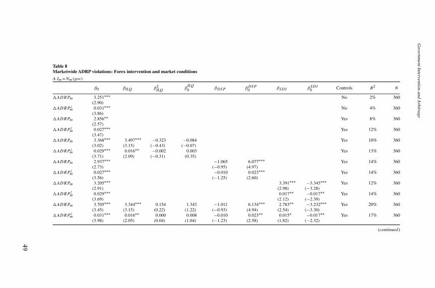
[14:5219/7/2017

RF

S-hhx074.tex]

Page:49

1–65

Governm

entInterventionand

Arbitrage

Table 8Marketwide ADRP violations: Forex intervention and market conditions

A.Im =Nm (gov)

β0 βILQ β2ILQ β

ILQ0 βDSP βDSP0 βSDI βSDI0 Controls R2 N

�ADRPm 3.251∗∗∗ No 2% 360(2.90)

�ADRPzm 0.031∗∗∗ No 4% 360(3.86)

�ADRPm 2.856∗∗ Yes 8% 360(2.57)

�ADRPzm 0.027∗∗∗ Yes 12% 360(3.47)

�ADRPm 3.368∗∗∗ 3.497∗∗∗ −0.323 −0.084 Yes 10% 360(3.02) (3.15) (−0.43) (−0.07)

�ADRPzm 0.029∗∗∗ 0.016∗∗ −0.002 0.003 Yes 13% 360(3.71) (2.09) (−0.31) (0.35)

�ADRPm 2.937∗∗∗ −1.065 6.077∗∗∗ Yes 14% 360(2.73) (−0.95) (4.97)

�ADRPzm 0.027∗∗∗ −0.010 0.023∗∗∗ Yes 14% 360(3.56) (−1.25) (2.60)

�ADRPm 3.205∗∗∗ 3.391∗∗∗ −3.345∗∗∗ Yes 12% 360(2.91) (2.98) (−3.28)

�ADRPzm 0.029∗∗∗ 0.017∗∗ −0.017∗∗ Yes 14% 360(3.69) (2.12) (−2.39)

�ADRPm 3.705∗∗∗ 3.344∗∗∗ 0.154 1.343 −1.011 6.134∗∗∗ 2.783∗∗ −3.232∗∗∗ Yes 20% 360(3.45) (3.15) (0.22) (1.22) (−0.93) (4.94) (2.54) (−3.30)

�ADRPzm 0.031∗∗∗ 0.016∗∗ 0.000 0.008 −0.010 0.023∗∗ 0.015∗ −0.017∗∗ Yes 17% 360(3.98) (2.05) (0.04) (1.04) (−1.23) (2.58) (1.82) (−2.32)

(continued )

49

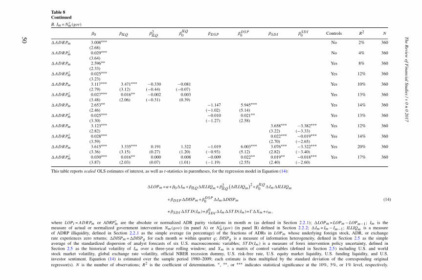
[14:5219/7/2017

RF

S-hhx074.tex]

Page:50

1–65

The

Review

ofFinancialStudies

/v0

n0

2017Table 8Continued

B. Im =Nzm (gov)

β0 βILQ β2ILQ β

ILQ0 βDSP βDSP0 βSDI βSDI0 Controls R2 N

�ADRPm 3.008∗∗∗ No 2% 360(2.68)

�ADRPzm 0.029∗∗∗ No 4% 360(3.64)

�ADRPm 2.596∗∗ Yes 8% 360(2.33)

�ADRPzm 0.025∗∗∗ Yes 12% 360(3.23)

�ADRPm 3.117∗∗∗ 3.471∗∗∗ −0.330 −0.081 Yes 10% 360(2.79) (3.12) (−0.44) (−0.07)

�ADRPzm 0.027∗∗∗ 0.016∗∗ −0.002 0.003 Yes 13% 360(3.48) (2.06) (−0.31) (0.39)

�ADRPm 2.653∗∗ −1.147 5.945∗∗∗ Yes 14% 360(2.46) (−1.02) (5.14)

�ADRPzm 0.025∗∗∗ −0.010 0.021∗∗ Yes 13% 360(3.30) (−1.27) (2.58)

�ADRPm 3.123∗∗∗ 3.658∗∗∗ −3.382∗∗∗ Yes 12% 360(2.82) (3.22) (−3.33)

�ADRPzm 0.028∗∗∗ 0.022∗∗∗ −0.019∗∗∗ Yes 14% 360(3.59) (2.70) (−2.65)

�ADRPm 3.615∗∗∗ 3.335∗∗∗ 0.191 1.322 −1.019 6.003∗∗∗ 3.076∗∗∗ −3.322∗∗∗ Yes 20% 360(3.36) (3.15) (0.27) (1.20) (−0.93) (5.12) (2.82) (−3.40)

�ADRPzm 0.030∗∗∗ 0.016∗∗ 0.000 0.008 −0.009 0.022∗∗ 0.019∗∗ −0.018∗∗∗ Yes 17% 360(3.87) (2.03) (0.07) (1.01) (−1.19) (2.55) (2.40) (−2.60)

This table reports scaled OLS estimates of interest, as well as t-statistics in parentheses, for the regression model in Equation (14):

�LOPm =α+β0�Im+βILQ�ILLIQm+β2ILQ

(�ILLIQm

)2 +βILQ0 �Im�ILLIQm

+βDSP �DISPm+βDSP0 �Im�DISPm (14)

+βSDI�STD(Im)+β0SDI�Im�STD(Im)+��Xm+εm,

where LOPt =ADRPm or ADRPzm are the absolute or normalized ADR parity violations in month m (as defined in Section 2.2.1); �LOPm =LOPm−LOPm−1; Im is themeasure of actual or normalized government intervention Nm (gov) (in panel A) or Nzm (gov) (in panel B) defined in Section 2.2.2; �Im =Im−Im−1; ILLIQm is a measureof ADRP illiquidity, defined in Section 2.2.1 as the simple average (in percentage) of the fractions of ADRs in LOPm whose underlying foreign stock, ADR, or exchangerate experiences zero returns; �DISPm =�DISPq for each month m within quarter q; DISPq is a measure of information heterogeneity, defined in Section 2.5 as the simpleaverage of the standardized dispersion of analyst forecasts of six U.S. macroeconomic variables; STD(Im) is a measure of forex intervention policy uncertainty, defined inSection 2.5 as the historical volatility of Im over a three-year rolling window; and Xm is a matrix of control variables (defined in Section 2.5) including U.S. and worldstock market volatility, global exchange rate volatility, official NBER recession dummy, U.S. risk-free rate, U.S. equity market liquidity, U.S. funding liquidity, and U.S.investor sentiment. Equation (14) is estimated over the sample period 1980–2009; each estimate is then multiplied by the standard deviation of the corresponding originalregressor(s). N is the number of observations; R2 is the coefficient of determination. ∗, ∗∗, or ∗∗∗ indicates statistical significance at the 10%, 5%, or 1% level, respectively.

50

[14:52 19/7/2017 RFS-hhx074.tex] Page: 51 1–65


each scaled coefficient in Table 8 is in the same unit as the dependent variable�LOPm.

The evidence in Table 8 provides additional support for my model. First,the estimated positive contemporaneous impact of forex intervention on ADRparity violations (β0>0) is robust to the inclusion of controls for changesin market conditions potentially related to limits to arbitrage and/or forexintervention activity as well as to the exclusion of its lead-lag effects, forexample, ranging between 2.6 bps (t =2.33; panel B) and 2.9 bps (t =2.57;panel A) in correspondence with a one-standard-deviation shock to �Im.Augmenting Equation (14) with additional control variables related to suchalternative sources of relative mispricings as marketwide financial distress,dislocations, foreign equity flows, or capital account liberalizations in emergingmarkets (e.g., Edison and Warnock 2003; Hu, Pan, and Wang 2013; Pasquariello2008, 2014; Brusa, Ramadorai, and Verdelhan 2015), when available, yieldsqualitatively similar inference. See, for example, Tables IA-10 to IA-13 in theInternet Appendix.

Second, estimates of βILQ in Table 8 are always positive and botheconomically and statistically significant. Consistent with Corollary 2 (e.g.,Figure 2A [solid line])—but also with the literature on arbitrage trading costsas determinants of LOP violations in general, andADRP violations in particular(see, e.g., Gagnon and Karolyi 2010; Gromb and Vayanos 2010)—deterioratingADRP liquidity is accompanied by larger ADRP violations (e.g., by as much as16% of the sample standard deviation of�LOPm) even in the absence of forexintervention. I nonetheless find no evidence of the potential nonmonotonicity inthis relation also hinted by Corollary 2 (e.g., Figure 2A [dashed line]): β2

ILQ ≈0in panels A and B of Table 8. Shocks to the average fraction of zero returnsdo not weaken, yet only weakly magnify the impact of forex interventions onADR parity violations: Estimates of β0 remain large and significant; estimatesof β ILQ

0 are often positive, consistent with H3, but small and never significant.However, the total effect ofADRPilliquidity alone on the relation between forexinterventions and ADRP violations (β0 +β ILQ

0 ) is both positive and large, forexample, about 18% of the baseline scaled estimates of β0 in Table 8. Relatedly,amending Equation (14) to include the interaction of �Im and (�ILLIQm)2

reveals some nonmonotonicity in the sensitivity of β0 to ADRP illiquidity(β ILQ

0 ), as hinted by Table 6. Likewise, as noted in Section 2.4, this evidence—in Table IA-14 in the Internet Appendix—cannot be explained by the model(i.e., via H3; e.g., Figure 2B), and may be related to other concurrent limits toADRP liquidity provision and trading (e.g., such as those in Xm); yet it doesnot otherwise affect the inference.

When I allow each of the components of my measure of ADRP illiquidity,ILLIQm (ZFOR

m , Zm, and ZFXm ) in Equation (14), its estimates in Table IA-15in the Internet Appendix suggest that, consistent with the literature, illiquidityin the U.S. market for international cross-listings (�Zm) is a more important

51

[14:52 19/7/2017 RFS-hhx074.tex] Page: 52 1–65


determinant of ADRP violations than illiquidity in the foreign markets for theunderlying stocks (�ZFOR

t ; e.g., Pasquariello 2008, 2014; Gagnon and Karolyi2010). The interaction of �Zm with forex intervention intensity (�Im) is alsogenerally positive and statistically significant, as postulated by the model (H3;e.g., Figure 2B). The effect of forex illiquidity (�ZFXt ) on ADRP violations isinstead weaker and its cross-product with�Im has more difficult interpretation,since both my model and many extant studies find forex interventions to havea significant impact on the liquidity of the targeted currencies (e.g., Bossaertsand Hillion 1991; Vitale 1999; Naranjo and Nimalendran 2000; Pasquariello2007b, 2010). Accordingly, the samplewide correlation between �ZFXt andeither �Nm (gov) or �Nz

m (gov) is weakly negative, consistent with the model(λ∗<λ in Section 1.2) and potentially weakening the estimated aggregateinteraction effect β ILQ

0 in Table 8. Nevertheless, the inference from Equation(14) is otherwise unaffected.

Third, the relation between forex interventions and ADRP violations issensitive to more direct measures of the specific determinants of marketliquidity in the model. In particular, forex intervention has a significantlygreater impact on ADRP violations in correspondence with greater dispersionof beliefs among market participants: βDSP

0 >0, as predicted by my model(H4; e.g., Figure 1B). For instance, ceteris paribus, a large increase in thenumber of interventions in a month (i.e., a one-standard-deviation shockto �Nm (gov)>0) is accompanied by more than three times larger ADRPviolations when information heterogeneity is high in that month (i.e., inconjunction with a one-standard-deviation shock to �DISPm), that is, bynearly 10 bps (β0 +βDSP

0 =3.705+6.134, in panel A of Table 8) versus anunconditional average increase of less than 3 bps (β0 =2.856). Estimates ofβDSP are instead always negative, but small and statistically insignificant,suggesting that the positive direct effect of information heterogeneity on theextent of LOPviolations postulated in Corollary 2 may be subsumed by changesin other market conditions in Equation (14). Therefore, the total joint effect of�Im and �DISPm alone on �LOPm (β0 +βDSP +βDSP0 ) is still positive andmore than twice as large, on average, as the baseline effect of �Im alone (β0)in Table 8.

Fourth, scaled estimates of the policy uncertainty coefficient βSDI inEquation (14) are always positive, statistically significant, and almost aslarge as (or larger than) the corresponding coefficient for the intensity offorex intervention β0. For example, panel B of Table 8 shows that a one-standard-deviation increase in normalized forex policy uncertainty in a month(�STD

[Nzm (gov)

]>0) is accompanied by between 12% and 17% greater ADR

parity violations in that month than their sample variation in Table 1, consistentwith my model (H5; e.g., Figure 1F), even in the absence of an increase in thestandardized number of forex interventions (�Nz

m (gov)=0). Estimates of theinteraction coefficient βSDI0 are, however, negative, suggesting that the positiveimpact of historical intervention volatility on ADRP violations (βSDI >0) is

52

[14:52 19/7/2017 RFS-hhx074.tex] Page: 53 1–65


weaker in months when intervention policy uncertainty may have been partiallyresolved by further intervention activity. Nonetheless, the total joint effect ofgreater intervention intensity and policy uncertainty alone on ADRP violations(β0 +βSDI +βSDI0 ) remains positive and between 6% and 31% larger than thecorresponding baseline scaled estimates of β0, in line with H5.

Alternatively, some studies argue that government intervention in currencymarkets may reflect actual and expected violations of the absolute purchasingpower parity (APPP, a relation between exchange rates and inflation ratesequating currency-adjusted prices of goods and services across countries),especially during periods of relatively high inflation (e.g., Naranjo andNimalendran 2000; Sarno and Taylor 2001; Neely 2005). Thus, the lattermay proxy for intensity and uncertainty in the former. However, inflationdifferentials are relatively low over my sample period. In addition, large APPPviolations often stem from multilateral international agreements (e.g., the Plazaand Louvre Accords in the 1980s), and hence may not translate into moreintense and uncertain intervention activity. I use monthly CPI inflation datafrom the Organisation for Economic Co-operation and Development (OECD)to compute the actual or historically normalized average or three-year rollingvolatility of absolute percentage APPP violations in the exchange rates targetedby government interventions in Table 2 (see, e.g., Bekaert and Hodrick 2012).These variables are often positively, yet weakly correlated to my measures offorex intervention intensity (�Im) and forex policy uncertainty (�STD(Im)),including during the portion of the sample when inflation differentials acrosscountries were the highest (1980–1989). Accordingly, estimates of Equation(14) when replacing�STD(Im) with shocks to APPP violation intensity yieldsnoisier but qualitatively similar inference. See, for example, Figure IA-5 andTables IA-16 and IA-17 in the Internet Appendix.

3. Conclusions

In this study, I propose and report evidence of the novel notion that directgovernment intervention in a market may induce LOP violations in other,arbitrage-related markets.

I illustrate the intuition for this negative externality of policy in two steps.I first construct a standard multiasset model of strategic, heterogeneouslyinformed speculation, based on Kyle (1985) and Chowdhry and Nanda(1991), in which segmentation in the dealership sector, speculative market-order trading, and less-than-perfectly correlated noise trading yield less-than-perfectly correlated equilibrium prices of two fundamentally identical, orlinearly related assets (i.e., equilibrium LOP violations). I then introduce astylized government pursuing a nonpublic, partially informative price targetfor only one of the two assets and consider the equilibrium implications ofits policy-motivated, camouflaged trading activity. I show that, given existinglimits to arbitrage, such intervention lowers those assets’ equilibrium price

53

[14:52 19/7/2017 RFS-hhx074.tex] Page: 54 1–65


correlation (i.e., increases equilibrium LOP violations) by clouding dealers’inference about the targeted asset’s payoff, with an intensity that depends in acomplex manner on extant price formation.

My empirical analysis provides support for this effect. I find that moreintense forex intervention activity between 1980 and 2009 is accompaniedby meaningfully larger LOP violations in the arbitrage-linked, yet arguablyless-than-perfectly integrated U.S. market for ADRs, but not in the arbitrage-linked, yet arguably perfectly integrated international money markets forexchange-risk-covered deposits and loans. This estimated relation is unaffectedby changes in market conditions typically associated with level and dynamicsof LOP violations, limits to arbitrage, and/or forex intervention. I also findit to be stronger for ADRs from both emerging economies and high-qualitymarkets, as well as in correspondence with low or deteriorating liquidity inthe ADR arbitrage-linked markets, greater dispersion of U.S. macroeconomicforecasts, and greater uncertainty about official currency policy, consistent withmy model.

These findings suggest that direct government intervention—an increasinglypopular policy tool in the aftermath of the recent financial crisis—may notonly yield welfare gains but also have nontrivial, undesirable implications forfinancial market quality. This is an important insight both for the understandingof the forces driving price formation, hence resource allocation and risksharing, in financial markets and for the debate on optimal financial policyand regulation.

Appendix

Proof of Proposition 1. The proof is by construction and proceeds in three steps (e.g., Kyle1985; Pasquariello and Vega 2009). In the first, I conjecture general linear functions for prices andtrading strategies. In the second, I solve for the parameters of those functions satisfying Conditions1 and 2 in Section 1.1. In the third, I verify that those parameters and functions represent arational expectations equilibrium. I begin by assuming that, in equilibrium, p1,i =A0,i +A1,iωi andxi (m)=B0,i +B1,i δv (m), where A1,i >0 and i = {1,2}. These assumptions and the definitions ofδv (m) and ωi imply that:

E[p1,i |δv (m)

]=A0,i +A1,ixi (m)+A1,iB0,i (M−1)+A1,iB1,i (M−1)ρδv (m). (A1)

Using Equation (A1), maximization of each speculator’s expected profit E [π (m)|δv (m)] withrespect to xi (m) yields the following first-order conditions:

0=p0 +δv (m)−A0,i−(M+1)A1,iB0,i−A1,iB1,i δv (m)[2+(M−1)ρ]. (A2)

The second-order conditions are satisfied, since −2A1,i <0. Equation (A2) is true iff:

p0 −A0,i =(M+1)A1,iB0,i , (A3)

2A1,iB1,i =1−(M−1)A1,iB1,iρ. (A4)

Because of the distributional assumptions in Section 1.1, ωi are normally distributedwith means E (ωi )=MB0,i , variances var (ωi )=MB2

1,iρσ2v [1+(M−1)ρ]+σ 2

z , and covariances

54

[14:52 19/7/2017 RFS-hhx074.tex] Page: 55 1–65


cov(v,ωi )=MB1,iρσ2v . It then ensues from the properties of conditional normal distributions (e.g.,

Greene 1997, p. 90) that:

E (v|ωi )=p0 +MB1,iρσ

2v

MB21,iρσ

2v [1+(M−1)ρ]+σ 2

z

(ωi−MB0,i

). (A5)

According to Condition 2 (semi-strong market efficiency), p1,i =E (v|ωi ). Therefore, the priorconjectures for p1,i are correct iff:

A0,i =p0 −MA1,iB0,i , (A6)

A1,i =MB1,iρσ

2v

MB21,iρσ

2v [1+(M−1)ρ]+σ 2

z

. (A7)

The expressions for A0,i , A1,i , B0,i , and B1,i in Proposition 1 must solve the system made ofEquations (A3), (A4), (A6), and (A7) to constitute a linear equilibrium. Defining A1,iB0,i fromEquation (A3) and plugging it into Equation (A6) leads to A0,i =p0. Since A1,i >0, only B0,i =0satisfies Equation (A3). Next, I solve Equation (A4) for A1,i :

A1,i =1

B1,i [2+(M−1)ρ]. (A8)

Equating Equation (A7) to Equation (A8) implies that B21,i =

σ2z

Mρσ2v

, i.e., that B1,i = σzσv

√Mρ

. I then

substitute this expression back into Equation (A8), yieldingA1,i = σv√Mρ

σz[2+(M−1)ρ] , and defineλ≡A1,i .Lastly, I follow Caballé and Krishnan (1994) to note that the equilibrium of Proposition 1 withM speculators is equivalent to a symmetric n-firm Cournot equilibrium. As such, the “backwardreaction mapping” technique in Novshek (1984) proves that, given a linear pricing rule (like theone of Equation (1)), the symmetric linear strategies xi (m) of Equation (2) represent the uniqueBayesian-Nash equilibrium of the Bayesian game among speculators. �

Proof of Corollary 1. The equilibrium pricing rule of Equation (1) implies that var(p1,i )=λ2var(ωi ) and covar(p1,1,p1,2)=λ2covar(ω1,ω2), where var(ωi )=σ 2

z [2+(M−1)ρ] andcovar(ω1,ω2)=σzz+σ 2

z [1+(M−1)ρ]. It is then straightforward to substitute these momentsinto the expression for the unconditional correlation of the equilibrium prices p1,1 and p1,2,

corr(p1,1,p1,2)=covar(p1,1,p1,2)√var(p1,1)var(p1,2)

, so yielding Equation (3). Under perfectly integrated market

making, MMs observe the aggregate order flow in both assets 1 and 2. Condition 2 (semi-strongmarket efficiency) then implies that p1,1 =E(v|ω1,ω2)=p1,2 (e.g., Caballé and Krishnan 1994,p. 697) and corr(p1,1,p1,2)=1. Under (less-than-) perfectly correlated noise trading, σzz =σ 2

z

(σzz <σ 2z ). Equation (3) then implies that corr(p1,1,p1,2)=1 (corr(p1,1,p1,2)<1). �

Proof of Corollary 2. Given the distributional assumptions in Section 1.1 (and σzz≥0), thestatement stems from observing that under less-than-perfectly correlated noise trading (σzz <

σ 2z ):

∂corr(p1,1,p1,2)∂ρ

=σ2z (M−1)(σ2

z −σzz)

[2+(M−1)ρ]2>0,

∂corr(p1,1,p1,2)

∂σ2z

=− σzz

σ4z [2+(M−1)ρ]

≤0,∂corr(p1,1,p1,2)

∂M=

σ2z ρ(σ2

z −σzz)

[2+(M−1)ρ]2>0, and

∂corr(p1,1,p1,2)∂σzz

= 1σ2z [2+(M−1)ρ]

>0. �

Proof of Proposition 2. As noted above, the proof is by construction. Its outline is based onPasquariello and Vega (2009) and Pasquariello, Roush, and Vega (2014). First, I conjecturelinear functions for equilibrium prices and the trading activity of speculators (in assets 1 and2) and the stylized government of Equation (4) (in asset 1 alone): p1,i =A0,i +A1,iωi , xi (m)=B0,i +B1,i δv(m), where A1,i >0 and i = {1,2}, and x1(gov)=C0,1 +C1,1δv(gov)+C2,1δT (gov).

55

[14:52 19/7/2017 RFS-hhx074.tex] Page: 56 1–65


Since E[δv(gov)|δv(m)]=ψδv(m) and E[δT (gov)|δv(m)]=δv(m) under the parametrization inSection 1.2, these conjectures imply that:

E[p1,1|δv (m)

]=A0,1 +A1,1x1 (m)+A1,1B0,1 (M−1)+A1,1B1,1 (M−1)ρδv (m)

+A1,1C0,1 +A1,1C1,1ψδv (m)+A1,1C2,1δv (m), (A9)

E[p1,2|δv (m)

]=A0,2 +A1,2x2 (m)+A1,2B0,2 (M−1)

+A1,2B1,2 (M−1)ρδv (m), (A10)

E[p1,1|δv (gov),δT (gov)

]=A0,1 +MA1,1B0 +MA1,1B1,1ρδv (gov)+A1,1x1 (gov). (A11)

Given Equations (A9) and (A10), the first-order conditions for maximizing each speculator’sexpected profit E [π (m)|Sv (m)] relative to xi (m) are:

0=p0 +δv (m)−A0,1 −(M+1)A1,1B0,1 −A1,1B1,1δv (m)[2+(M−1)ρ]

−A1,1C0,1 −A1,1C1,1ψδv (m)−A1,1C2,1δv (m), (A12)

0=p0 +δv (m)−A0,2 −(M+1)A1,2B0,2 −A1,2B1,2δv (m)[2+(M−1)ρ]. (A13)

Because −2A1,i <0, the second-order conditions are satisfied. For Equations (A12) and (A13) tobe true, it must be that:

p0 −A0,1 = (M+1)A1,1B0,1 +A1,1C0,1, (A14)

2A1,1B1,1 =1−(M−1)A1,1B1,1ρ−A1,1C1,1ψ−A1,1C2,1, (A15)

p0 −A0,2 = (M+1)A1,2B0,2, (A16)

2A1,2B1,2 =1−(M−1)A1,2B1,2ρ. (A17)

The government’s optimal intervention strategy is the one minimizing its expected loss functionof Equation (4), E[L(gov)|δv(gov),δT (gov)], with respect to x1(gov). Given the distributionalassumptions of Sections 1.1. and 1.2, removing all terms not interacting with the latter from theformer implies that x1(gov)=argminE[L(gov)|δv(gov),δT (gov)] is equal to:

argmin[γA2

1,1x21 (gov)+2γA2

1,1MB0,1x1 (gov)+2γA21,1MB0,1ρδv (gov)x1 (gov)

+2γA0,1A1,1x1 (gov)−2γpT1,1A1,1x1 (gov)+(1−γ )A0,1x1 (gov) (A18)

+(1−γ )A1,1x21 (gov)+(1−γ )MA1,1B0,1x1 (gov)

+(1−γ )MA1,1B1,1ρδv (gov)x1 (gov)−(1−γ )p0x1 (gov)−(1−γ )δv (gov)x1 (gov)].

The first-order condition from Equation (A18) is:

0=2γA21,1x1 (gov)+2γA2

1,1MB0,1 +2γA21,1MB0,1ρδv (gov)+2γA0,1A1,1 −2γpT1,1A1,1

+(1−γ )A0,1 +2(1−γ )A1,1x1 (gov)+(1−γ )MA1,1B0,1 (A19)

+(1−γ )MA1,1B1,1ρδv (gov)−(1−γ )p0 −(1−γ )δv (gov).

56

[14:52 19/7/2017 RFS-hhx074.tex] Page: 57 1–65


The second-order condition is satisfied, since 2γA21,1 +2(1−γ )A1,1>0. Let us define d≡ γ

1−γ .Given Equation (A19), the prior conjecture for x1 (gov) is then correct iff:

p0 −A0,1 =2A1,1C0,1 +MA1,1B0,1 +2dA21,1C0,1

+2dA21,1MB0,1 +2dA0,1A1,1 −2dpT1,1A1,1, (A20)

2A1,1C1,1 =1−MA1,1B1,1ρ−2dA21,1C1,1 −2dA2

1,1MB1,1ρ, (A21)

A1,1C2,1 =dA1,1 −dA21,1C2,1. (A22)

Equation (A22) implies that C2,1 = d1+dA1,1

>0. The prior conjectures for xi (m) and x1 (gov) also

imply that the aggregate order flows ω1 and ω2 are normally distributed with means E (ω1)=MB0,1 +C0,1 and E (ω2)=MB0,2, the following variances:

var (ω1)=MB21,1ρσ

2v [1+(M−1)ρ]+C2

1,1ψσ2v +C2

2,1σ 2v

μψ

+2MB1,1C1,1ψρσ2v +2MB1,1C2,1ρσ

2v +2C1,1C2,1σ

2v +σ 2

z , (A23)

var (ω2)=MB21,2ρσ

2v [1+(M−1)ρ]+σ 2

z , (A24)

and covariances cov(v,ω1)=MB1,1ρσ2v +C1,1ψσ

2v +C2,1σ

2v and cov(v,ω2)=MB1,2ρσ

2v . From the

market-clearing Condition 2 (p1,i =E(v|ωi )), it then ensues that:

p1,1 =p0 +

(MB1,1ρ+C1,1ψ +C2,1

)σ 2v

σ 2z +σ 2

v

{MB2

1,1ρ [1+(M−1)ρ]+D1 +E1

} (ω1 −MB0,1 −C0,1

), (A25)

p1,2 =p0 +MB1,2ρσ

2v

MB21,2ρσ

2v [1+(M−1)ρ]+σ 2

z

(ω2 −MB0,2

), (A26)

whereD1 =2Mρ[B1,1(ψC1,1 +C2,1)] and E1 =ψC21,1 + 1

μψC2

2,1 +2C1,1C2,1. Thus, the conjecturesfor p1,i are true iff

A0,1 =p0 −MA1,1B0,1 −A1,1C0,1, (A27)

A1,1 =

(MB1,1ρ+C1,1ψ +C2,1

)σ 2v

σ 2z +σ 2

v

{MB2

1,1ρ [1+(M−1)ρ]+D1 +E1

} , (A28)

A0,2 =p0 −MA1,2B0,2, (A29)

A1,2 =MB1,2ρσ

2v

MB21,2ρσ

2v [1+(M−1)ρ]+σ 2

z

. (A30)

Next, I verify that the expressions forA0,i ,A1,i , B0,i , B1,i , C0,1, and C1,1 in the linear equilibriumof Proposition 2 solve the system made of Equations (A14) to (A17), (A20), (A21), and (A27)to (A30). As shown in the proof of Proposition 1, Equations (A16), (A17), (A29), and (A30)

imply that B0,2 =0, A0,2 =0, B1,2 = σzσv

√Mρ

, and A1,2 = σv√Mρ

σz[2+(M−1)ρ] . For both Equations (A14)

and (A27) to be true, it must be that B0,1 =0. Because of the latter, Equation (A14) implies thatp0 −A0,1 =A1,1C0,1. Substituting A1,1C0,1 into Equation (A20) yields A0,1 =p0 +2dA1,1

57

[14:52 19/7/2017 RFS-hhx074.tex] Page: 58 1–65


(p0 −pT1,1) and C0,1 =2d(pT1,1 −p0). I am left to find A1,1, B1,1, and C1,1. I first extract B1,1

from Equation (A15) and C1,1 from Equation (A21):

B1,1 =1−A1,1C1,1ψ−A1,1C2,1

A1,1 [2+(M−1)ρ], (A31)

C1,1 =1−MA1,1B1,1ρ

(1+2dA1,1

)2A1,1

(1+dA1,1

) . (A32)

I then solve the system made of Equations (A31) and (A32) to get B1,1 = 2−ψA1,1f (A1,1) >0 and

C1,1 =[2+(M−1)ρ](1+dA1,1)−Mρ(1+2dA1,1)

A1,1(1+dA1,1)f (A1,1) , where f (A1,1)=2[2+(M−1)ρ](1+dA1,1)−Mψρ(1+

2dA1,1) is clearly positive. Lastly, I substitute these expressions for B1,1 and C1,1 in Equation(A28), yielding a sextic polynomial in A1,1,

g1,6A61,1 +g1,5A

51,1 +g1,4A

41,1 +g1,3A

31,1 +g1,2A

21,1 +g1,1A1,1 +g0,1 =0, (A33)

whose coefficients can be shown to be (via tedious algebra and the parameter restrictions inSections 1.1 and 1.2):

g0,1 =−μψσ 2v

[Mρ (2−ψ)2 +ψ (2−ρ)2

]<0, (A34)

g1,1 =−2μψσ 2v d

{Mρ

[2(2−ψ)−ψ2 (1−ρ)−ρψ

]+2ψ (2−ρ)2

}<0, (A35)

g2,1 =μψσ 2z

{4(2−ρ)2 +Mρ

[Mρ (2−ψ)2 +4(2−ρ)(2−ψ)

]}

+σ 2v d

2{

4(1−μψ)(2−ρ)2 +4Mρ [Mρ (1−ψ)+2(2−ψ−ρ)+ψρ] (A36)

+4μψρ[3M (ρ+ψ)−M

(7+ρψ +ρψ2

)+5ψ

]

+M2ρ2ψ [μψ (11−4ψ)+ψ−8μ]+μψ2 [ρ (7Mψ−5ρ)−20]},

g3,1 =2σ 2v d

3{

(2−ρ)2[4(1−μψ)−μψ2

]+Mρ (2−ρ)

[μψ

(7ψ−10+ψ2

)

+2(4−3ψ)]+2M2ρ2[μψ2 (5−2ψ)−ψ (3−ψ)+(2−3μψ)

]}(A37)

+2μψσ 2z d

{8(2−ρ)2 +M2ρ2 [8−ψ (10−3ψ)]+2Mρ (2−ρ)(8−5ψ)

},

g4,1 =4(1−μψ)σ 2v d

4 [(2−ρ)+Mρ (1−ψ)]2

+μψσ 2z d

2{

12(2−ρ)[2(2−ρ)+Mρ (4−3ψ)]+M2ρ2 [24+ψ (13ψ−36)]}>0, (A38)

g5,1 =4μψσ 2z d

3{M2ρ2 [4−ψ (7−3ψ)]+Mρ [16−7ψ (2−ρ)−8ρ]+4(2−ρ)2

}>0, (A39)

g6,1 =4μψσ 2z d

4 [Mρ (1−ψ)+(2−ρ)]2>0, (A40)

where either sign(g3,1)= sign(g2,1)= sign(g1,1), sign(g4,1)= sign(g3,1)= sign(g2,1), or sign(g4,1)=sign(g3,1) and sign(g2,1)= sign(g1,1), such that only one change of sign is possible while proceeding

58

[14:52 19/7/2017 RFS-hhx074.tex] Page: 59 1–65


from the lowest to the highest power term in the polynomial of Equation (A33). According toDescartes’ rule, under these conditions there exists only one positive real root λ∗ of Equation(A33). Hence, this root implies the unique linear Bayesian Nash equilibrium of Proposition 2. ByAbel’s impossibility theorem, Equation (A33) cannot be solved with rational operations and finiteroot extractions. In the numerical examples of Figure 1, I find λ∗ using the three-stage algorithmproposed by Jenkins and Traub (1970a, 1970b) under some mild restrictions on exogenousparameter values to ensure its convergence to a solution, for example, such that the government is“reasonably committed” to a “reasonably uncertain” policy target pT (i.e., γ is sufficiently lowerthan 1, while ψ and μ are sufficiently higher than 0). �

Proof of Corollary 3. As for the proof of Corollary 1, I start by observing that corr(p∗1,1,p

∗1,2)=

covar(p∗1,1,p

∗1,2)√

var(p∗1,1)var(p∗

1,2), where Equations (5) and (6) imply that var(p∗

1,1)=λ∗2var(ω∗1), var(p∗

1,2)=

λ2var(ω∗2), and covar(p∗

1,1,p∗1,2)=λλ∗covar(ω∗

1,ω∗2). Because of the distributional assumptions

of Sections 1.1 and 1.2, it is straightforward to show that var(ω∗1)=σ 2

z +σ 2v {MρB∗2

1,1[1+(M−1)ρ]+D∗

1 +E∗1 }, var(ω∗

2)=σ 2z [2+(M−1)ρ], and covar(ω∗

1,ω∗2)=σzz+σzσv

√Mρ{B∗

1,1[1+(M−1)ρ]+ψC∗

1,1 +C∗2,1}. Substituting these expressions into the one for corr(p∗

1,1,p∗1,2) yields Equation

(10). Once again, if MMs observe order flow in both assets 1 and 2, Condition 2 (semi-strongmarket efficiency) implies that p∗

1,1 =E(v|ω∗1,ω

∗2)=p∗

1,2 (e.g., Caballé and Krishnan 1994, p. 697)and corr(p∗

1,1,p∗1,2)=1. �

References

Acharya, V., and M. Richardson, eds. 2009. Restoring financial stability: How to repair a failed system—Anindependent view from New York University Stern School of Business. Hoboken, NJ: John Wiley & Sons.

Adrian, T., E. Etula, and T. Muir. 2014. Financial intermediaries and the cross section of asset returns. Journalof Finance 69:2557–96.

Albuquerque, R., and C. Vega. 2009. Economic news and international stock market co-movement. Review ofFinance 13:401–65.

Allen, H., and M. Taylor. 1990. Charts, noise, and fundamentals in the foreign exchange market. EconomicJournal 29:49–59.

Andersen, T., and T. Bollerslev. 1998. Deutsche mark-dollar volatility: Intraday activity patterns, macroeconomicannouncements, and longer run dependencies. Journal of Finance 53:219–65.

Andersen, T., T. Bollerslev, F. Diebold, and C. Vega. 2003. Micro effects of macro announcements: Real-timeprice discovery in foreign exchange. American Economic Review 93:38–62.

———. 2007. Real-time price discovery in stock, bond, and foreign exchange markets. Journal of InternationalEconomics 73:251–77.

Auguste, S., K. Dominguez, H. Kamil, and L. Tesar. 2006. Cross-border trading as a mechanism for capital flight:ADRs and the Argentine crisis. Journal of Monetary Economics 53:1259–95.

Baker, M., and J. Wurgler. 2006. Investor sentiment and the cross-section of stock returns. Journal of Finance61:1645–80.

———. 2007. Investor sentiment and the stock market. Journal of Economic Perspectives 21:129–51.

Baker, M., J. Wurgler, and Y. Yuan. 2012. Global, local, and contagious investor sentiment. Journal of FinancialEconomics 104:272–87.

Bank for International Settlements (BIS). 2016. Report on global foreign exchange market activity in 2016.Triennial Central Bank Survey.

59

[14:52 19/7/2017 RFS-hhx074.tex] Page: 60 1–65


Baruch, S., A. Karolyi, and M. Lemmon. 2007. Multimarket trading and liquidity: Theory and evidence. Journalof Finance 62:2169–200.

Beber, A., M. Brandt, and M. Luisi. 2014. Distilling the macroeconomic news flow. Working Paper, DukeUniversity.

Beine, M., C. Bos, and S. Laurent. 2007. The impact of central bank FX interventions on currency components.Journal of Financial Econometrics 5:154–83.

Beine, M., G. Janssen, and C. Lecourt. 2009. Should central bankers talk to the foreign exchange markets?Journal of International Money and Finance 28:776–803.

Beine, M., S. Laurent, and F. Palm. 2009. Central bank forex interventions assessed using realized moments.Journal of International Financial Markets, Institutions & Money 19:112–27.

Bekaert, G., and C. Harvey. 1995. Time-varying world market integration. Journal of Finance 50:403–44.

———. 1997. Emerging equity market volatility. Journal of Financial Economics 43:29–78.

———. 2000. Foreign speculators and emerging equity markets. Journal of Finance 55:565–613.

———. 2003. Emerging markets finance. Journal of Empirical Finance 10:3–55.

Bekaert, G., C. Harvey, and C. Lundblad. 2007. Liquidity and expected returns: Lessons from emerging markets.Review of Financial Studies 20:1783–831.

Bekaert, G., C. Harvey, and A. Ng. 2005. Market integration and contagion. Journal of Business 75:39–69.

Bekaert, G., and R. Hodrick. 2012. International financial management. Upper Saddle River, NJ: Pearson-PrenticeHall.

Bernanke, B. 2012. Monetary policy since the onset of the crisis. Remarks delivered at the Jackson Hole EconomicSymposium, Federal Reserve Bank of Kansas City.

Bhattacharya, U., and P. Weller. 1997. The advantage of hiding one’s hand: Speculation and central bankintervention in the foreign exchange market. Journal of Monetary Economics 39:251–77.

Bond, P., and I. Goldstein. 2015. Government intervention and information aggregation by prices. Journal ofFinance 70:2777–811.

Bonser-Neal, C., V. Roley, and G. Sellon. 1998. Monetary policy actions, intervention, and exchange rates:A reexamination of the empirical relationships using federal funds rate target data. Journal of Business 71:147–77.

Bossaerts, P., and P. Hillion. 1991. Market microstructure effects of government intervention in the foreignexchange market. Review of Financial Studies 4:513–41.

Boulatov, A., T. Hendershott, and D. Livdan. 2013. Informed trading and portfolio returns. Review of EconomicStudies 80:35–72.

Brunetti, C., M. di Filippo, and J. Harris. 2011. Effects of central bank intervention on the interbank marketduring the subprime crisis. Review of Financial Studies 24:2053–83.

Brusa, F., T. Ramadorai, and A. Verdelhan. 2015. The international CAPM redux. Working Paper, MIT.

Caballé, J., and M. Krishnan. 1994. Imperfect competition in a multi-security market with risk neutrality.Econometrica 62:695–704.

———. 2004. Asset prices, order flows and the sources of volatility with insider trading. Working Paper,Universidad Autonoma de Barcelona.

Chen, N., R. Roll, and S. Ross. 1986. Economic forces and the stock market. Journal of Business 59:383–403.

Chordia, T., J. Hu, A. Subrahmanyam, and Q. Tong. 2017. Order flow volatility and equity costs of capital.Working Paper, Emory University.

60

[14:52 19/7/2017 RFS-hhx074.tex] Page: 61 1–65


Chordia, T., and A. Subrahmanyam. 2004. Order imbalance and individual stock returns: Theory and evidence.Journal of Financial Economics 72:485–518.

Chortareas, G., Y. Jiang, and J. Nankervis. 2013. Volatility and spillover effects of yen interventions. Review ofInternational Economics 21:671–89.

Chowdhry, B., and V. Nanda. 1991. Multimarket trading and market liquidity. Review of Financial Studies4:483–511.

Coffey, N., W. Hrung, H. Nguyen, and A. Sarkar. 2009. The global financial crisis and offshore dollar markets.FRBNY Current Issues in Economics and Finance 15:1–7.

Cong, Y., R. Hoitash, and M. Krishnan. 2010. Event study with imperfect competition and private information:Earnings announcements revisited. Review of Quantitative Finance and Accounting 34:383–411.

Corrigan, G., and R. Davis. 1990. Intermediate targets and indicators for monetary policy: A critical survey.New York: Federal Reserve Bank of New York.

Croushore, D. 1993. Introducing: The survey of professional forecasters. Business Review, Federal Reserve Bankof Philadelphia, 3–15.

D’Amico, S., and T. King. 2013. Flow and stock effects of large-scale treasury purchases: Evidence on theimportance of local supply. Journal of Financial Economics 108:425–48.

Diether, K., C. Malloy, and A. Scherbina. 2002. Differences of opinion and the cross-section of stock returns.Journal of Finance 57:2113–41.

Dimson, E. 1979. Risk measurement when shares are subject to infrequent trading. Journal of FinancialEconomics 7:197–226.

Dominguez, K. 2003. The market microstructure of central bank intervention. Journal of International Economics59:25–45.

———. 2006. When do central bank interventions influence intra-daily and longer-term exchange ratemovements? Journal of International Money and Finance 25:1051–71.

Dominguez, K., and J. Frankel. 1993. Does foreign exchange intervention matter? The portfolio effect. AmericanEconomic Review 83:1356–69.

Dovern, J., U. Fritsche, and J. Slacalek. 2012. Disagreement among forecasters in G7 countries. Review ofEconomics and Statistics 94:1081–96.

Dufey, G., and I., Giddy. 1994. The international money market. Upper Saddle River, NJ: Pearson-Prentice Hall.

Dyck, A., and A. Morse. 2011. Sovereign wealth fund portfolios. Working Paper, University of Chicago.

Edison, H. 1993. The effectiveness of central-bank intervention: A survey of the literature after 1982. SpecialPapers in International Economics 18:1–63.

Edison, H., and F. Warnock. 2003. A simple measure of the intensity of capital controls. Journal of EmpiricalFinance 10:81–103.

Eichler, S., A. Karmann, and D. Maltritz. 2009. The ADR shadow exchange rate as an early warning indicatorfor currency crises. Journal of Banking and Finance 33:1983–95.

Engel, C. 2014. Exchange rates and interest parity, In Handbook of international economics, eds. Gopinath, G.,E. Helpman, and K. Rogoff. Amsterdam: Elsevier.

Evans, M., and R. Lyons. 2002. Order flow and exchange rate dynamics. Journal of Political Economy 110:170–80.

———. 2005. Are different-currency assets imperfect substitutes? In Exchange rate economics: Where do westand? ed. De Grauwe, P. Cambridge, MA: MIT Press.

———. 2013. Exchange rate fundamentals and order flow. Quarterly Journal of Finance 2:1–63.

61

[14:52 19/7/2017 RFS-hhx074.tex] Page: 62 1–65


Fatum, R., and M. Hutchison. 2003. Is sterilised foreign exchange intervention effective after all? An event studyapproach. Economic Journal 113:390–411.

Fischer,A., and M. Zurlinden. 1999. Exchange rate effects of central bank interventions:An analysis of transactionprices. Economic Journal 109:662–76.

Foucault, T., and T. Gehrig. 2008. Stock price informativeness, cross-listings, and investment decisions. Journalof Financial Economics 88:146–68.

Foucault, T., M. Pagano, and A. Röell. 2013. Market liquidity: Theory, evidence, and policy. Oxford: OxfordUniversity Press

Fratzscher, M. 2006. On the long-term effectiveness of exchange rate communication and interventions. Journalof International Money and Finance 25:146–67.

Frenkel, J., and R. Levich. 1975. Covered interest arbitrage: Unexploited profits. Journal of Political Economy83:325–38.

———. 1977. Transaction costs and interest arbitrage: Tranquil versus turbulent periods. Journal of PoliticalEconomy 85:1209–26.

Gagnon, L., andA. Karolyi. 2010. Multi-market trading and arbitrage. Journal of Financial Economics 97:53–80.

Garleanu, N., and L. Pedersen. 2011. Margin-based asset pricing and deviations from the law of one price. Reviewof Financial Studies 24:1980–2022.

Gerlach-Kristen, P., R. McCauley, and K. Ueda. 2016. Currency intervention and the global portfolio balanceeffect: Japanese lessons. Journal of the Japanese and International Economies 39:1–16

Green, C. 2004. Economic news and the impact of trading on bond prices. Journal of Finance 59:1201–33.

Greene, W. 1997. Econometric analysis. Upper Saddle River, NJ: Pearson-Prentice Hall.

Griffoli, T., and A. Ranaldo. 2011. Limits to arbitrage during the crisis: Funding liquidity constraints and coveredinterest parity. Working Paper, Swiss National Bank.

Gromb, D., and D. Vayanos. 2010. Limits to arbitrage: The state of the theory. Annual Review of FinancialEconomics 2:251–75.

Hamilton, J. 1994. Time series analysis. Princeton, NJ: Princeton University Press.

Hanson, S., A. Kashyap, and J. Stein. 2011. A macroprudential approach to financial regulation. Journal ofEconomic Perspectives 25:3–28.

Harvey, C., and R. Huang. 2002. The impact of the Federal Reserve Bank’s open market operations. Journal ofFinancial Markets 5:223–57.

Hasbrouck, J. 1991. Measuring the information content of stock trades. Journal of Finance 46:179–207.

———. 2007. Empirical market microstructure. New York: Oxford University Press.

Hassan, T., T. Mertens, and T. Zhang. 2016. Currency manipulation. Working Paper, NBER.

Hong, S. 2016. The quiet side of China’s market intervention. Wall Street Journal, January 13, 2016.https://www.wsj.com/articles/chinas-national-team-plays-defense-when-stocks-decline-1452686207.

Hu, X., J. Pan, and J. Wang. 2013. Noise as information for illiquidity. Journal of Finance 68:2341–82.

Humpage, O., and W. Osterberg. 1992. Intervention and the foreign exchange risk premium: An empiricalinvestigation of daily effects. Global Finance Journal 3:23–50.

Ince, O., and R. Porter. 2006. Individual equity return data from Datastream: Handle with care! Journal ofFinancial Research 29:463–79.

Jansen, D., and J. De Haan. 2005. Talking heads: The effects of ECB statements on the euro-dollar exchangerate. Journal of International Money and Finance 24:343–61.

62

https://www.wsj.com/articles/chinas-national-team-plays-defense-when-stocks-decline-1452686207

[14:52 19/7/2017 RFS-hhx074.tex] Page: 63 1–65


Jenkins, M., and J. Traub. 1970a. A three-stage variables-shift iteration for polynomial zeros and its relation togeneralized Rayleigh iteration. Numerishe Mathematik 14:252–63.

———. 1970b.Athree-stage algorithm for real polynomials using quadratic iteration. SIAM Journal of NumericalAnalysis 7:545–66.

Jones, C., G. Kaul, and M. Lipson. 1994. Transactions, volume, and volatility. Review of Financial Studies7:631–51.

Kaminsky, G., and K. Lewis. 1996. Does foreign exchange intervention signal future monetary policy? Journalof Monetary Economics 37:285–312.

Karolyi,A. 1998. Why do companies list shares abroad?Asurvey of the evidence and its managerial implications.Financial Markets, Institutions & Instruments 7:1–60.

———. 2006. The world of cross-listings and cross-listings of the world: Challenging conventional wisdom.Review of Finance 10:73–115.

Karolyi, A., and Y. Wu. Forthcoming. A partial segmentation model of international stock returns. Journal ofFinancial and Quantitative Analysis.

Kyle, A. 1985. Continuous auctions and insider trading. Econometrica 53:1315–35.

Lamont, O., and R. Thaler. 2003. Anomalies: The law of one price in financial markets. Journal of EconomicPerspectives 17:191–202.

Lesmond, D. 2005. Liquidity of emerging markets. Journal of Financial Economics 77:411–52.

Lesmond, D., J. Ogden, and C. Trzcinka. 1999. A new estimate of transaction costs. Review of Financial Studies12:1113–41.

Levy Yeyati, E., S. Schmukler, and N. Van Horen. 2009. International financial integration through the law ofone price: The role of liquidity and capital controls. Journal of Financial Intermediation 18:432–63.

Lewis, K. 1995. Occasional intervention to target rates. American Economic Review 85:691–715.

Lyons, R. 2001. The microstructure approach to exchange rates. Cambridge: MIT Press.

Lyons, R., and M. Moore. 2009. An information approach to international currencies. Journal of InternationalEconomics 79:211–21.

Madhavan, A. 2000. Market microstructure: A survey. Journal of Financial Markets 3:205–58.

Mancini, L., A. Ranaldo, and J. Wrampelmeyer. 2013. Liquidity in the foreign exchange market: Measurement,commonality, and risk premiums. Journal of Finance 68:1805–41.

McKinnon, R. 1977. The eurocurrency market. In Essays in international finance, ed. R. McKinnon. Princeton,NJ: Princeton University.

Menkhoff, L. 2010. High-frequency analysis of foreign exchange interventions: What do we learn? Journal ofEconomic Surveys 24:85–112.

Naranjo,A., and M. Nimalendran. 2000. Government intervention and adverse selection costs in foreign exchangemarkets. Review of Financial Studies 13:453–77.

Neely, C. 2000. The practice of central bank intervention: Looking under the hood. Central Banking 11:24–37.

———. 2005. An analysis of recent studies of the effect of foreign exchange intervention. Federal Reserve Bankof St. Louis Review 87:685–717.

———. 2006. Identifying the effects of U.S. intervention on the levels of exchange rates. Working Paper, FederalReserve Bank of St. Louis.

Neely, C., and P. Weller. 2007. Central bank intervention with limited arbitrage. International Journal of Financeand Economics 12:249–60.

63

[14:52 19/7/2017 RFS-hhx074.tex] Page: 64 1–65


Novshek, W. 1984. Finding all n-firm Cournot equilibria. International Economic Review 25:61–70.

O’Hara, M. 1995. Market microstructure theory. Malden, MA: Blackwell.

Pasquariello, P. 2007a. Imperfect competition, information heterogeneity, and financial contagion. Review ofFinancial Studies 20:391–426.

———. 2007b. Informative trading or just costly noise? An analysis of central bank interventions. Journal ofFinancial Markets 10:107–43.

———. 2008. The anatomy of financial crises: Evidence from the emergingADR market. Journal of InternationalEconomics 76:193–207.

———. 2010. Central bank intervention and the intraday process of price formation in the currency markets.Journal of International Money and Finance 29:1045–61.

———. 2014. Financial market dislocations. Review of Financial Studies 27:1868–1914.

Pasquariello, P., and C. Vega. 2007. Informed and strategic order flow in the bond markets. Review of FinancialStudies 20:1975–2019.

———. 2009. The on-the-run liquidity phenomenon. Journal of Financial Economics 92:1–24.

Pasquariello, P., J. Roush, and C. Vega. 2014. Government intervention and strategic trading in the U.S. treasurymarket. Working Paper, University of Michigan.

Pastor, L., and R. Stambaugh. 2003. Liquidity risk and expected stock returns. Journal of Political Economy111:642–85.

Pastor, L., and P. Veronesi. 2012. Uncertainty about government policy and stock prices. Journal of Finance67:1219–64.

———. 2013. Political uncertainty and risk premia. Journal of Financial Economics 110:520–45.

Payne, R., and P. Vitale. 2003. A transaction level study of the effects of central bank intervention on exchangerates. Journal of International Economics 61:331–52.

Peiers, B. 1997. Informed traders, intervention and price leadership: A deeper view of the microstructure of theforeign exchange market. Journal of Finance 52:1589–1614.

Pelizzon, L., M. Subrahmanyam, D. Tomio, and J. Uno. 2016. Sovereign credit risk, liquidity, and EuropeanCentral Bank intervention: Deus ex machina? Journal of Financial Economics 122:86–115.

Pontiff, J. 1996. Costly arbitrage: Evidence from closed-end funds. Quarterly Journal of Economics 111:1135–51.

———. 2006. Costly arbitrage and the myth of idiosyncratic risk. Journal of Accounting and Economics 42:35–52.

Rogoff, K. 1985. The optimal degree of commitment to an intermediate monetary target. Quarterly Journal ofEconomics 100:1169–89.

Sarkissian, S., and M. Schill. 2016. Cross-listing waves. Journal of Financial and Quantitative Analysis 51:259–306.

Sarno, L., and M. Taylor. 2001. Official intervention in the foreign exchange market: Is it effective, and if so,how does it work? Journal of Economic Literature 39:839–68.

Shleifer, A. 2000. Inefficient markets: An introduction to behavioral finance. Oxford: Oxford University Press.

Shleifer, A., and R. Vishny. 1997. The limits of arbitrage. Journal of Finance 52:35–55.

Sojli, E., and W. Tham. 2010. The impact of foreign government investments on corporate performance: Evidencefrom the U.S. Working Paper, Erasmus University.

Stein, J., 1989. Cheap talk and the Fed: A theory of imprecise policy announcements. American Economic Review79:32–42.

64

[14:52 19/7/2017 RFS-hhx074.tex] Page: 65 1–65


Subrahmanyam, A. 1991a. A theory of trading in stock index futures. Review of Financial Studies 4:17–51.

———. 1991b. Risk aversion, market liquidity, and price efficiency. Review of Financial Studies 4:417–41.

Taylor, D. 1982. Official intervention in the foreign exchange market, or, bet against the central bank. Journalof Political Economy 90:356–68.

Ulrich, M. 2010. How does the bond market perceive FOMC interventions? Working Paper, Columbia University.

Vitale, P. 1999. Sterilised foreign exchange intervention in the foreign exchange market. Journal of InternationalEconomics 49:245–67.

Vives, X. 2008. Information and learning in markets. Princeton, NJ: Princeton University Press.

Witmer, J. 2008. An examination of Canadian firms delisting from U.S. exchanges. Working Paper, Bank ofCanada.

Xie, J. 2009. From bonding to avoiding: Evidence from ADR delisting. Working Paper, RavenPack.

Yu, J. 2011. Disagreement and return predictability of stock portfolios. Journal of Financial Economics 99:162–83.

65

government intervention and arbitrage

Documents