gpf: a f f g p c o gpu c -p
TRANSCRIPT

GPF: A FRAMEWORK FOR GENERAL PACKETCLASSIFICATION ON GPU CO-PROCESSORS
Submitted in fulfilmentof the requirements of the degree of
MASTER OF SCIENCE
of Rhodes University
Alastair Nottingham
Grahamstown, South AfricaOctober 2011

Abstract
This thesis explores the design and experimental implementation of GPF, a novelprotocol-independent, multi-match packet classification framework. This frame-work is targeted and optimised for flexible, efficient execution on NVIDIA GPUplatforms through the CUDA API, but should not be difficult to port to other plat-forms, such as OpenCL, in the future.
GPF was conceived and developed in order to accelerate classification of largepacket capture files, such as those collected by Network Telescopes. It uses a multi-phase SIMD classification process which exploits both the parallelism of packetsets and the redundancy in filter programs, in order to classify packet capturesagainst multiple filters at extremely high rates. The resultant framework - com-prised of classification, compilation and buffering components - efficiently lever-ages GPU resources to classify arbitrary protocols, and return multiple filter re-sults for each packet.
The classification functions described were verified and evaluated by testing anexperimental prototype implementation against several filter programs, of varyingcomplexity, on devices from three GPU platform generations. In addition to thesignificant speedup achieved in processing results, analysis indicates that the pro-totype classification functions perform predictably, and scale linearly with respectto both packet count and filter complexity. Furthermore, classification throughput(packets/s) remained essentially constant regardless of the underlying packet data,and thus the effective data rate when classifying a particular filter was heavily in-fluenced by the average size of packets in the processed capture.
For example: in the trivial case of classifying all IPv4 packets ranging in size from70 bytes to 1KB, the observed data rate achieved by the GPU classification kernelsranged from 60Gbps to 900Gbps on a GTX 275, and from 220Gbps to 3.3Tbps on aGTX 480. In the less trivial case of identifying all ARP, TCP, UDP and ICMP pack-ets for both IPv4 and IPv6 protocols, the effective data rates ranged from 15Gbpsto 220Gbps (GTX 275), and from 50Gbps to 740Gbps (GTX 480), for 70B and 1KBpackets respectively.

Acknowledgements
I would like to thank my supervisor, Dr. Barry Irwin, who provided tremendoussupport and guidance throughout the course of this research, and my co-supervisorfrom DPSS, Joey van Vuuren, who provided both valuable support and funding forthis research. In addition, I would like to thank Jeremy Baxter of the RhodesUniversity Department of Statistics, who sacrificed his own free time to help withthe analysis of the performance results. Finally, I would like to thank my family,for everything they have to done to help make this research possible.
This work was performed in and funded by the Centre of Excellence in DistributedMultimedia at Rhodes University, with financial support from Telkom SA, Com-verse, Verso Technologies, Tellabs, StorTech, EastTel and THRIP. Funding for GPUequipment was also received from the National Research Foundation Thutuka Pro-gram, via my supervisor thought Grant number 69018. Thanks are also expressedto Defense Peace Safety and Security (DPSS) unit of the Council for Scientific andIndustrial Research (CSIR) for providing generous funding to me for the degree.

Contents
1 Introduction 1
1.1 Network Telescopes . . . . . . . . . . . . . . . . . . . . . . . . . . . . . 2
1.2 Problem statement . . . . . . . . . . . . . . . . . . . . . . . . . . . . . 3
1.3 Research Method . . . . . . . . . . . . . . . . . . . . . . . . . . . . . . 5
1.4 Scope . . . . . . . . . . . . . . . . . . . . . . . . . . . . . . . . . . . . . 5
1.5 Summary of Goals . . . . . . . . . . . . . . . . . . . . . . . . . . . . . . 6
1.6 Additional Notes . . . . . . . . . . . . . . . . . . . . . . . . . . . . . . . 7
1.7 Document Structure . . . . . . . . . . . . . . . . . . . . . . . . . . . . 7
2 Packet Filters 8
2.1 Packets . . . . . . . . . . . . . . . . . . . . . . . . . . . . . . . . . . . . 9
2.2 Packet Headers . . . . . . . . . . . . . . . . . . . . . . . . . . . . . . . 10
2.3 Packet Filters . . . . . . . . . . . . . . . . . . . . . . . . . . . . . . . . 14
2.4 Target Hardware . . . . . . . . . . . . . . . . . . . . . . . . . . . . . . 18
2.5 Algorithms for IP Processing . . . . . . . . . . . . . . . . . . . . . . . 22
2.6 Protocol-Independent Algorithms . . . . . . . . . . . . . . . . . . . . . 36
2.7 Summary . . . . . . . . . . . . . . . . . . . . . . . . . . . . . . . . . . . 41
i

CONTENTS ii
3 Graphics Processing Units 43
3.1 General Purpose Computation on GPUs . . . . . . . . . . . . . . . . . 44
3.2 CUDA Hardware Model . . . . . . . . . . . . . . . . . . . . . . . . . . 47
3.3 CUDA Programming Model . . . . . . . . . . . . . . . . . . . . . . . . 50
3.4 Memory Regions . . . . . . . . . . . . . . . . . . . . . . . . . . . . . . 53
3.5 Data Transfer Optimisation . . . . . . . . . . . . . . . . . . . . . . . . 58
3.6 Improving Processing Efficiency . . . . . . . . . . . . . . . . . . . . . . 63
3.7 Packet Filtering Considerations . . . . . . . . . . . . . . . . . . . . . 66
3.8 Summary . . . . . . . . . . . . . . . . . . . . . . . . . . . . . . . . . . . 70
4 GPU Accelerated Packet Classification 72
4.1 Introduction to GPF . . . . . . . . . . . . . . . . . . . . . . . . . . . . . 73
4.2 Processing Packets in Parallel . . . . . . . . . . . . . . . . . . . . . . 76
4.3 Rule Evaluation . . . . . . . . . . . . . . . . . . . . . . . . . . . . . . . 83
4.4 Evaluating Filters . . . . . . . . . . . . . . . . . . . . . . . . . . . . . . 91
4.5 High-Level Grammar . . . . . . . . . . . . . . . . . . . . . . . . . . . . 95
4.6 Packet Collection and Buffering . . . . . . . . . . . . . . . . . . . . . . 101
4.7 Analysis Extensions . . . . . . . . . . . . . . . . . . . . . . . . . . . . 108
4.8 Future Functionality . . . . . . . . . . . . . . . . . . . . . . . . . . . . 110
4.9 Summary . . . . . . . . . . . . . . . . . . . . . . . . . . . . . . . . . . . 114

CONTENTS iii
5 Evaluation and Testing 116
5.1 Testing Configuration . . . . . . . . . . . . . . . . . . . . . . . . . . . . 117
5.2 Verification . . . . . . . . . . . . . . . . . . . . . . . . . . . . . . . . . . 122
5.3 Timing Results Validation . . . . . . . . . . . . . . . . . . . . . . . . . 125
5.4 Packet Throughput . . . . . . . . . . . . . . . . . . . . . . . . . . . . . 133
5.5 Filter Program Performance . . . . . . . . . . . . . . . . . . . . . . . . 139
5.6 Performance Comparison . . . . . . . . . . . . . . . . . . . . . . . . . . 150
5.7 Summary . . . . . . . . . . . . . . . . . . . . . . . . . . . . . . . . . . . 155
6 Conclusion 157
6.1 Future Work . . . . . . . . . . . . . . . . . . . . . . . . . . . . . . . . . 160
6.2 Other Applications . . . . . . . . . . . . . . . . . . . . . . . . . . . . . 161
Bibliography 162
A GPF Filter Programs 173
A.1 IP Protocols (IPP) . . . . . . . . . . . . . . . . . . . . . . . . . . . . . . 173
A.2 Single Simple Filter (SSF) . . . . . . . . . . . . . . . . . . . . . . . . . 174
A.3 Multiple Simple Filter (MSF) . . . . . . . . . . . . . . . . . . . . . . . 174
A.4 Single Compound Filter (SCF) . . . . . . . . . . . . . . . . . . . . . . . 174
A.5 Multiple Compound Filters (MCF) . . . . . . . . . . . . . . . . . . . . 175
A.6 Large Simple Filters (LSF) . . . . . . . . . . . . . . . . . . . . . . . . . 175
B List of Publications 179
C Contents of Multimedia DVD 181

List of Figures
2.1 Example TCP/IP packet, decomposed into its abstract layers. . . . . 10
2.2 Stack level traversal when transmitting a packet to a remote hostusing the TCP/IP model. . . . . . . . . . . . . . . . . . . . . . . . . . . 12
2.3 Layer comparison between the OSI and TCP/IP models. . . . . . . . . 13
2.4 Example Set Pruning Tree created from the filter set shown in Table2.1. Adapted from [78]. . . . . . . . . . . . . . . . . . . . . . . . . . . 25
2.5 Grid-of-Tries structure, equivalent to the Set Pruning Tree shown inFigure 2.4. Adapted from [78]. . . . . . . . . . . . . . . . . . . . . . . 26
2.6 Geometric representation of a 2-dimensional filter over 4-bit addressand port fields. Adapted from [78]. . . . . . . . . . . . . . . . . . . . . 28
2.7 Hierarchical Intelligent Cuttings data-structure applied to filters de-picted in Figure 2.6. Adapted from [78]. . . . . . . . . . . . . . . . . . 29
2.8 Example of Modular Packet Classification using the filter set shownin Table 2.2. Adapted from [78]. . . . . . . . . . . . . . . . . . . . . . 30
2.9 Example Parallel Bit-Vector classification structure over the filtersdepicted in Figure 2.6. Adapted from [78]. . . . . . . . . . . . . . . . 32
2.10 Example Crossproducting algorithm. Adapted from [78]. . . . . . . . 34
2.11 Example P 2C range encoding, matching the port values (y-axis) ofthe filters depicted in Figure 2.6. Adapted from [78]. . . . . . . . . . 35
iv

LIST OF FIGURES v
2.12 Timeline of protocol-independent packet filters. . . . . . . . . . . . . . 37
2.13 Example high-level Control Flow Graph checking for a reference to ahost “foo”. Adapted from [50]. . . . . . . . . . . . . . . . . . . . . . . . 38
3.1 Abstract overview of the NVIDIA GTX 280. . . . . . . . . . . . . . . . 49
3.2 Coalescing global memory access for 32-bit words on the GTX 280. . 55
3.3 Synchronous execution versus asynchronous execution in memory-bound kernels. . . . . . . . . . . . . . . . . . . . . . . . . . . . . . . . . 60
3.4 Affect of thread block sizes on GTX 280 multiprocessor occupancy. . 64
3.5 Employing unroll-and-jam to reduce iteration overhead. . . . . . . . 65
3.6 Overview of Gnort NIDS. Adapted from [83]. . . . . . . . . . . . . . . 69
4.1 Abstract architecture of GPF. . . . . . . . . . . . . . . . . . . . . . . . 75
4.2 Synchronous vs. Streamed classification. . . . . . . . . . . . . . . . . 77
4.3 Memory layout comparison for 16 packets processing 4 rules. . . . . 80
4.4 High-level memory architecture of the Rule kernel. . . . . . . . . . . 83
4.5 Geometric proof that 32-bit Rule fields span no more than two con-secutive 32-bit integers. . . . . . . . . . . . . . . . . . . . . . . . . . . 85
4.6 Iterative Rule evaluation. . . . . . . . . . . . . . . . . . . . . . . . . . 86
4.7 Example extraction of a field spanning both cache integers. . . . . . . 89
4.8 Iterative predicate evaluation. . . . . . . . . . . . . . . . . . . . . . . . 92
4.9 Precedence hierarchy in parenthesis-free predicate evaluation. . . . 92
4.10 Filter code representation of the predicate in Figure 4.9. . . . . . . . 95
4.11 Overview of the GPF compilation process. . . . . . . . . . . . . . . . 99
4.12 Peak theoretical transfer rate comparison. . . . . . . . . . . . . . . . 104

LIST OF FIGURES vi
4.13 Example effects of edge cropping optimisation on packet size. . . . . 106
4.14 Comparative WinPcap dumpfile filtering times for HDD vs. RAMdisk. . . . . . . . . . . . . . . . . . . . . . . . . . . . . . . . . . . . . . 107
4.15 Dividing a 128-bit IPv6 address field into multiple sub-fields. . . . . 111
5.1 Mean completion time of the IP Filter program. . . . . . . . . . . . . 127
5.2 Absolute σ of performance validation tests, in milliseconds. . . . . . . 128
5.3 Relative σ of performance validation tests, as a percentage of the mean.129
5.4 Host component timing results for 107 packets over 100 iterations. . 130
5.5 CUDA component timing results for 107 packets over 100 iterations. 131
5.6 Percentage of processing time spent performing component functions. 134
5.7 Execution time against packet count for all three packet sets. . . . . 135
5.8 Single Simple Filter (SSF) program performance. . . . . . . . . . . . 140
5.9 Multiple Simple Filter (MSF) program performance. . . . . . . . . . . 142
5.10 Single Compound Filter (SCF) program performance. . . . . . . . . . 145
5.11 Multiple Compound Filters (MCF) program performance. . . . . . . . 147
5.12 Large Simple Filter program performance. . . . . . . . . . . . . . . . 149
5.13 Comparison of estimated performance . . . . . . . . . . . . . . . . . . 154

List of Tables
2.1 Example Filter Set, showing source and destination IP address pre-fixes for each filter. Adapted from [78]. . . . . . . . . . . . . . . . . . . 25
2.2 Example filter set, containing 4-bit port and address values. Adaptedfrom [78]. . . . . . . . . . . . . . . . . . . . . . . . . . . . . . . . . . . . 27
3.1 Configurations and compute capabilities of various GPUs. . . . . . . 48
3.2 Keywords for thread identification. . . . . . . . . . . . . . . . . . . . . 52
3.3 GTX 280 memory regions. . . . . . . . . . . . . . . . . . . . . . . . . . 53
5.1 Technical comparison of test graphics card specifications. . . . . . . . 119
5.2 Packet sets used in testing. . . . . . . . . . . . . . . . . . . . . . . . . 120
5.3 Results of regression analysis . . . . . . . . . . . . . . . . . . . . . . . 138
5.4 Projected packets per hour and filtering rates for varying averagepacket size. . . . . . . . . . . . . . . . . . . . . . . . . . . . . . . . . . . 139
5.5 Predicted Single Simple Filter (SSF) throughput and resultant datarate for varying packet size. . . . . . . . . . . . . . . . . . . . . . . . . 141
5.6 Multiple Single Filters (MSF) program performance measurementsand comparison. . . . . . . . . . . . . . . . . . . . . . . . . . . . . . . . 143
5.7 Predicted Single Compound Filter (SCF) throughput and resultantdata rate for varying packet size. . . . . . . . . . . . . . . . . . . . . . 144
vii

LIST OF TABLES viii
5.8 Multiple Compound Filter (MCF) performance measurements andcomparison. . . . . . . . . . . . . . . . . . . . . . . . . . . . . . . . . . 146
5.9 Large Single Filter set performance measurements and comparison. 150
5.10 Observed data rate and throughput for RAM disk . . . . . . . . . . . 151
5.11 Derived Libtrace throughput and data rate for a simple BPF filter . 152
5.12 Comparative performance of different graphics cards for each filterprogram vs. GTX 275 results. . . . . . . . . . . . . . . . . . . . . . . . 155

List of Code Listings
1 Time difference between synchronous and asynchronous execution. . 612 Improving division and modulo performance. . . . . . . . . . . . . . . 663 EBNF for rule code . . . . . . . . . . . . . . . . . . . . . . . . . . . . . 874 Psuedocode for field extraction. . . . . . . . . . . . . . . . . . . . . . . 905 EBNF for Filter and Subfilter Code . . . . . . . . . . . . . . . . . . . . 946 EBNF for the GPF Grammar . . . . . . . . . . . . . . . . . . . . . . . 977 Example high-level filter program classifying packets against two
distinct port ranges. . . . . . . . . . . . . . . . . . . . . . . . . . . . . . 988 Example Decisional Execution . . . . . . . . . . . . . . . . . . . . . . . 1129 Hypothetical use of an IP protocol definition. . . . . . . . . . . . . . . 113
ix

1Introduction
PACKET classifiers, also known as packet filters, are ubiquitous componentsin modern networked environments, and are fundamental to many net-work, security and monitoring applications. These applications require
fast, efficient and flexible identification of both live packet streams and offlinepacket captures, in order to identify malicious activity, to analyse local traffic, andto facilitate network security related research [11, 38]. Packet classification is acomputationally expensive process, however, and achieving multi-gigabit classifi-cation rates is thus difficult without expensive, non-commodity hardware. Further-more, most modern algorithms target select protocol-specific fields, and therebysacrifice flexibility in order to meet the throughput demands of modern high-speednetworks.
This thesis describes the design and implementation of GPF (GPU Packet Filter):a flexible, protocol-independent, multi-match packet classifier, developed specifi-cally for execution on modern commodity NVIDIA GPU (Graphics Processing Unit)hardware. The development of GPF was primarily motivated by a need to ac-celerate the data-intensive analysis of large packet sets captured from Network
1

1.1. NETWORK TELESCOPES 2
Telescopes [38], which is often an extremely slow and tedious process when usingexisting Central Processing Unit (CPU) frameworks.
In the following section, the reader is introduced to Network Telescopes, and theoriginal motivation for developing a GPU classification algorithm. This sectionis provided to supply context for the work undertaken, and reflects only a singleinstance of a wider problem. The research problem statement which follows ap-proaches the problem from a more general perspective, and explains briefly theapproach adopted to address this problem.
1.1 Network Telescopes
Network telescopes are passive, low interaction traffic collectors (or sensors) whichare used extensively in the analysis of Internet Background Radiation (IBR). IBRconsists of non productive Internet traffic; for example, packets destined for ad-dresses that do not exist, or for servers which are either offline, or are not con-figured to receive the incoming transmission [65]. Network telescopes collect andrecord IBR packet traces by passively monitoring large segments of unused Inter-net Protocol (IP) address space, such as an otherwise unallocated large Class A(/8) or a small Class C (/24) network [38, 65]. As these segments are devoid ofhosts, there is no need to filter out productive traffic from the collected IBR, andlittle threat of a successful attack — besides packet floods or Distributed Denial ofService (DDoS) attacks — from external hosts.
Packets collected at network telescopes fall into one of three broad categories:backscatter, misconfigured transmissions, and aggressive or hostile traffic [38].Backscatter comprises benign nonproductive traffic transmitted in response to mis-configured or spoofed traffic that originated elsewhere, while misconfigured trans-missions are typically produced by badly configured hosts. The majority of IBRtraffic, however, is aggressive or potentially hostile [38], and includes TCP andICMP scans, UDP packets with malicious payloads, and other virus and malwarerelated activity. This malicious traffic, once captured, may be analysed to identifynew Internet-based vulnerabilities and threats, to determine the level of infectionof known malware, and to study the propagation dynamics of this malware overtime.

1.2. PROBLEM STATEMENT 3
Packets traces are collected by network telescopes over regular daily, weekly ormonthly intervals, and stored in Pcap dump files for later processing in networkanalysis tools such as WireShark1, TcpDump2 and Libtrace3 [38]. The number ofpackets in these traces is dependent on the interval of collection and the rate ofpacket arrival, which in turn is affected by the size of the telescope being used.While small (/24) telescopes typically only receive in the order of 1000 packets perhour, large Class A (/8) telescopes may receive several million. As a result, somelong term IBR captures may contain tens or hundreds of billions of packets, whichmay take hours or days to process [11]. When captures include productive trafficfrom active hosts in addition to IBR, these counts may grow by one or more ordersof magnitude, thereby making analysis of the captured data entirely impractical.
For instance, assuming an average packet arrival rate of 10 packets per IP addressper hour, a large Class A (/8) network telescope — with roughly 16.7 million ad-dresses — may expect to receive over 167 million packets every hour. This equatesto roughly 4 billion packets per day, 120 billion packets a month, and 1.4 trillionpackets per year. Given that Libtrace achieves a throughput of roughly 6 millionpackets per second when filtering for TCP traffic on port 80 [11], performing a simi-lar operation on 1.4 trillion packets would require almost three days. Consequently,analysing long-term traces collected from large telescopes can be an extremely slowand tedious process, which ultimately inhibits exploration and near-real-time anal-ysis of the captured telescope data.
For more information regarding the benefits and applications of network telescopes,the reader is encouraged to consult “A Framework for the Application of NetworkTelescope Sensors in a Global IP Network” by Barry Irwin [38].
1.2 Problem statement
Applications such as WireShark and Libtrace are often employed to diagnose anoma-lies, monitor and analyse traffic, and perform general network and security relatedresearch [10]. Many of these scenarios operate on live traffic or offline packet cap-tures collected from high-bandwidth networks with hundreds of active hosts. Such
1http://www.wireshark.org/download.html2http://www.tcpdump.org/3http://research.wand.net.nz/software/libtrace.php

1.2. PROBLEM STATEMENT 4
networks have the collective potential to generate tens of millions of packets persecond, which is significantly greater than the peak performance of either Libtraceor WireShark. This throughput limitation thus makes thorough, long term moni-toring and analysis of high-speed traffic impractical.
The most significant limiting factor affecting the throughput of these network anal-ysis tools is the underlying classification mechanism. This mechanism has tradi-tionally relied on the CPU of the host machine to provide the necessary flexibilityto classify any arbitrary protocol field, without requiring expensive, specialisedhardware. As CPUs are primarily sequential processors, packets are filtered oneat a time, resulting in a significant bottleneck when millions of packets are col-lected each second, and are classified against a non-trivial filter set. Consequently,protocol-independent classifiers match packets to only a single filter, in order tohelp reduce per packet filtering times.
While the protocol-independent packet classifiers used in network analysis toolsopt to process packets sequentially (so as to cater to the strengths of CPUs), packetclassification is itself a highly parallelisable process. As the order of packet ar-rival cannot be guaranteed, each incoming packet must be classified independentlyagainst a constant filter set, thereby allowing for parallelism at the packet level.The task of packet classification is thus potentially well-suited to massively paral-lel architecture, such as modern commodity GPUs. Unfortunately, existing protocol-independent packet classification algorithms are not easily ported to this medium,due to their heavy reliance on sequential optimisations that are extremely ineffi-cient when performed on GPU hardware. As a result, very little research existsregarding the utilisation of GPUs to perform this task.
This thesis details the design and implementation of GPF, a novel filtering ar-chitecture targeting Compute Unified Device Architecture (CUDA) enabled GPUco-processors explicitly, which has been developed, in part, to assess the potentialbenefit of GPUs in accelerating packet classification. This framework dramaticallyaccelerates the filtering process, and bridges the gap between filter throughputand modern high-bandwidth interface speeds. In addition, GPF returns resultsfor each filter independently, and allows for multiple overlapping filters to be runconcurrently, without obscuring potential results.

1.3. RESEARCH METHOD 5
1.3 Research Method
This research was undertaken to evaluate the viability of GPU accelerated pro-cessing to improve packet classification throughput, achieved through the methodof experimental synthesis. In essence, a classifier tailored to GPU hardware wasdesigned, and subsequently implemented as a functional prototype. This prototypewas then evaluated to measure its accuracy and performance over a range of testcases.
The design for this classifier was derived by considering a wide range of specialisedand general classification algorithms, in order to identify effective strategies whichmay be adapted, reconstituted and combined to effect an efficient GPU solution.This preliminary research, in combination with a relatively thorough review of theperformance characteristics of GPU devices, directed the conceptual developmentof both the GPU classification functions, and the classification system in general.With the exception of the GPU functions described, many architectural and tech-nical elements which support the classification process (such as packet bufferingand program compilation) have been discussed extensively elsewhere, and do notwarrant detailed exploration or extensive testing at this point.
A prototype implementation — modified to facilitate validation and performancemeasurement at a program component level — was utilised to evaluate the classi-fiers performance potential. The prototype implementation was modified to alloweach component of the system to measured independently, one at a time, both toaid in identifying any potential bottlenecks, and to ensure the measurements col-lected for classification functions were not skewed by the performance and resourceutilisation of other system components.
1.4 Scope
While the scope of the design presented in Chapter 4 includes discussion of all rel-evant GPU and CPU components, the primary focus of this work is developing andassessing the core classification process executed within the GPU context, and notto develop and test a complete classification system. The scope of implementationis thus limited to a functional prototype, capable of measuring the performance ofthe GPU classification functions.

1.5. SUMMARY OF GOALS 6
In order to test the primary filtering functionality being developed, the prototypesystem needs to accept both filter programs and packet data as input. Due to thisrequirement, the prototype facilitates both high-level filter compilation — whichconverts GPF filter specifications into instructions for the GPU classification func-tions — and packet collection from capture files. While support for filtering livenetwork interfaces will likely be incorporated in the future, this functionality hasbeen left out of scope for the time being, as it is not particularly useful when mea-suring classification performance. Packet capture files are better suited to this pur-pose, as, unlike live captures, they are not restricted by the speed of the interfacebeing processed, they may be accessed on demand, and they allow for independentverification of results. In addition, functions supporting packet analysis has beenleft out of scope, as their usefulness depends on the viability of the classificationmethod. Analytical extensions and future functionality are, however, briefly dis-cussed in the classifiers design.
Hence, while the prototype is essentially a functional classification system, it lacksmany of the optimisations and refinements described in the design to improve us-ability and component level performance. The prototype thus reflects a perfor-mance baseline for the GPU classification process, which is expected to be ex-panded and improved upon in future work.
1.5 Summary of Goals
In summary, the goal of this research is to determine the viability and usefulnessof GPU accelerated packet classification through the following method:
• Design a flexible classification framework, capable of classifying against mul-tiple arbitrary filters, that is optimised for efficient, parallel execution onGPU hardware.
• Implement a functional prototype of this framework which includes all GPUclassification functions and necessary supporting architecture.
• Evaluate the classification performance of this prototype to infer the potentialvalue of employing GPUs to accelerate packet classification.

1.6. ADDITIONAL NOTES 7
1.6 Additional Notes
• The terms packet classifier and packet filter are used interchangeably through-out this thesis, as they are largely treated as being synonymous in the Litera-ture. While the traditional term, packet filter, was used almost exclusively inearlier works, the arguably more accurate term, packet classifier, has becomeincreasingly prominent in recent years.
• This thesis depends heavily on references published online. While undesir-able, the cutting-edge nature of both the GPGPU field and the tools employedin this thesis made this difficult to avoid.
1.7 Document Structure
The remainder of this document is structured as follows:
• Chapter 2 introduces the domain of packet classification and its core concepts,and investigates a selection of diverse packet filter designs.
• Chapter 3 provides an introduction to NVIDIA GPU hardware, and examinesthe CUDA programming model and its performance characteristics in detail.The chapter concludes by considering why existing classification algorithms,such as those discussed in Chapter 2, would not perform efficiently on GPUhardware.
• Chapter 4 introduces the filtering strategy employed, and describes the high-level architecture of the GPF classification system, before providing designand implementation information for individual components.
• Chapter 5 presents the results of testing performed on a prototype implemen-tation of GPF, with specific focus on performance and accuracy.
• Chapter 6 concludes with a summary of research findings, a discussion possi-ble applications, and an overview of future work.

2Packet Filters
THIS chapter introduces the reader to the domain of packet filtering anda selection of existing IP-specific and protocol-independent filtering algo-rithms, in order to provide suitable context for the design of the GPF algo-
rithm presented in Chapter 4. The chapter is organised as follows:
• Section 2.1 begins with a brief introduction to the structure and use of packetsin digital networks.
• Section 2.2 details the role of packet headers in facilitating packet-based com-munication, and describes how packet headers are constructed in order tofulfill this role.
• Section 2.3 introduces the abstract filtering mechanisms employed to classifypackets using components of these headers, and details some of their variousattributes and properties.
• Section 2.4 considers four common programmable hardware mediums on whichpacket filters have been deployed, and how the capabilities of these mediumsare exploited in classifier design.
8

2.1. PACKETS 9
• Section 2.5 explores a diverse selection of IP-specific classification algorithms,which operate on the Internet Protocol exclusively in order to meet the packetthroughput demands imposed by modern high-bandwidth networks.
• Section 2.6 briefly examines several important protocol-independent packetfilter implementations, before concluding with a summary in Section 2.7.
Much of the content covered in this chapter was derived and expanded fromresearch previously published by the researcher in the proceedings of the2009 SAICSIT conference, South Africa [52].
2.1 Packets
Data is transferred between network interfaces contained within binary arraysknown as packets [50, 77]. Packets typically comprise a data segment — known asthe payload — combined with a series of protocol headers used for transmitting,routing and receiving packets. Packet sizes vary dramatically depending on theirpayload, function, protocol and transportation medium, but all protocols define aMaximum Transmission Unit (MTU) which specifies the maximum size a partic-ular packet type may be [68]. Some protocols, such as the Internet Protocol [68],allow payloads which exceed the MTU to be divided over multiple packets, termedfragments. Fragments may be reconstituted into a single payload by the receiv-ing host once they have arrived at their destination, achieved through the use offragment related information contained within the packet header [77].
Packet headers contain vast amounts of useful network-related data, including ad-dress and port information, protocol flags, and other information relevant to suc-cessful transmission [77, 78]. Packet classifiers use this information to rapidlycategorise incoming packets, and have been employed in a variety of domains, in-cluding packet routing between remote hosts [45, 76], demultiplexing incomingpacket streams [50], analysing packet set composition [38], providing network re-lated security through firewalls [49], and facilitating intrusion detection [83].

2.2. PACKET HEADERS 10
Figure 2.1: Example TCP/IP packet, decomposed into its abstract layers.
2.2 Packet Headers
Conceptually, packet headers are organised as a stack. Each level in the stack isassociated with a different type of service, and the stack is organised such thateach layer receives services from the layer directly below it, and provides servicesto the layer directly above it. The Transmission Control Protocol / Internet Protocol(TCP/IP) model, for instance, is divided between four broad layers, whereas theOpen Systems Interconnection (OSI) model is divided among seven discrete layers.This section introduces these models, and describes how they are used to facilitatethe transmission of packets between remote hosts.
2.2.1 The TCP/IP Model
TCP/IP, also known as the Internet Protocol Suite [22], is leveraged in the trans-mission of the vast majority of modern network traffic, and has been pivotal to thesuccess of the Internet. Although not an explicit design choice, TCP/IP may beviewed as a four layer stack, consisting of the Link Layer, Internet Layer, Trans-port Layer and Application Layer [69, 77]. A high-level overview of the structureof a TCP/IP packet mapped onto these four layers is provided in Figure 2.1.
The Link Layer is responsible for preparing packets for dispatch, as well as thephysical transmission of packets to a remote host or the next-hop router. Thislayer is only responsible for delivering a packet to the next router or host in thechain, and it is up to the receiving interface to direct the packet on to a router orhost closer to the transmission end-point. This process is repeated by each nodein the chain, until such time as the packet arrives at its destination. To achievethis, a frame header is added to the packet, containing the relevant information

2.2. PACKET HEADERS 11
to deliver the packet to the target host or the next-hop router over the specifiednetwork medium. As a result, the Link Layer is associated with protocols whichsupport this physical transmission, such as Ethernet II or WiFi (802.11 a/b/g/n).
The Internet Layer, located directly above the Link Layer in the TCP/IP stack,is responsible for the delivery of packets between end-points in a transmission.The Internet Layer’s functionality is contained within the Internet Protocol (IP),which facilitates logical, hierarchical end-point addressing through IP addresses,and enables packet routing by specifying the terminal node in the transmission.The Link Layer uses the address information encapsulated in IP, as well as routingtables, to derive the physical address of the next network interface between thesending and receiving host. In this way, the Link Layer provides a service to theInternet Layer by determining the delivery route a packet navigates to arrive atits remote destination, and transmitting it along that route. IP has two widelyused implementations, namely IP version 4 (IPv4), which supports just over fourmillion 32-bit addresses, and IP version 6 (IPv6), which uses 128-bit addresses thatprovide roughly 3.4× 1038 unique address values.
The Transport Layer is entirely independent of the underlying network [22, 77],and is responsible for ensuring that packets are delivered to the correct appli-cation through service ports. The two most common Transport Layer protocolsare the Transmission Control Protocol (TCP) [69] and the User Datagram Protocol(UDP) [67]. TCP is a connection-orientated protocol which addresses transmissionreliability concerns by:
• discarding duplicate packets
• ensuring lost or dropped packets are resent
• ensuring packet sequence is maintained
• checking for correctness and corruption through a 16 bit check-sum
In contrast, UDP is a connectionless protocol which provides only best-effort deliv-ery and weak error checking. Unlike TCP, UDP sacrifices reliability for efficiency[77], making it ideal for applications such as Domain Name Service (DNS) look-ups,where the overhead necessary for maintaining a connection is disproportionate tothe task itself.

2.2. PACKET HEADERS 12
Figure 2.2: Stack level traversal when transmitting a packet to a remote host usingthe TCP/IP model.
Both TCP and UDP define two 16-bit service ports, namely Source Port and Des-tination Port, which are used to determine which application a particular packetshould be delivered to. As has been noted, both TCP and UDP are network agnos-tic, and leave network related functionality to lower layers in the protocol stack[67, 69].
The top-most layer in the TCP/IP stack is the Application Layer, which simply en-capsulates the data to be delivered to the waiting application. This data may itselfcontain further application specific headers, which are handled by the receivingprocess. The packet is terminated by the Frame Footer, associated with the LinkLayer, which delimits the packet, and provides additional functionality such aserror checking.
Figure 2.2 illustrates the process by which a TCP/IP packet is transmitted froma sending host to a distant receiving host via two routers. When an applicationexecuting on the sending host wishes to transmit a payload to the receiving host,it descends the TCP stack, applying relevant headers to the payload at each level.First, the Application layer headers are applied, then the Transport Layer head-ers, and so on. Once all headers have been applied, the packet is transmitted tothe next-hop router, Router A. Router A receives the packet and, using informa-tion contained in the Internet Layer and routing tables, determines the shortestpath to the Receiving host. It then re-sends the packet with a new Link Layerheader, destined for Router B. Router B repeats this process, delivering the packet

2.2. PACKET HEADERS 13
Figure 2.3: Layer comparison between the OSI and TCP/IP models.
to the Receiving Host. The payload is then extracted and delivered to the waitingapplication by ascending the stack, removing headers at each layer.
2.2.2 The Open Systems Interconnect (OSI) Model
The OSI Model, a product of the International Organisation for Standardisation,is a seven layer standard model for network communication. Unlike the TCP/IPmodel, layering is both explicit and an integral part of the model’s design [5]. Inpractice, however, the OSI model’s seven explicit layers are functionally quite sim-ilar to the four general layers in the TCP/IP model, and provide the same basicservices. Due to this inherent similarity, it is possible to outline the OSI model interms of the TCP/IP model.
The seven layers defined by the OSI model, from lowest to highest, are the PhysicalLayer, Data-Link Layer, Network Layer, Transport Layer, Session Layer and Appli-cation Layer [5]. The Physical and Data-Link layers are essentially encapsulatedby the Link Layer of the TCP/IP stack, decomposing it into two distinct processes;physical transmission and packet framing. The Network layer is roughly equiv-alent to the Internet Layer of the TCP/IP model, although there is some overlapwith the TCP/IP Link Layer. Similarly, the Transport Layer, and a small subset ofthe Session layer, are contained within the Transport Layer of the TCP/IP model,

2.3. PACKET FILTERS 14
while the remainder of the Session Layer, as well as the Presentation and Applica-tion Layers are left as application specific data, contained within the ApplicationLayer of the TCP/IP Model. A diagrammatic representation of this breakdown isprovided in Figure 2.3.
While the TCP/IP model is considered exclusively from this point on, any discus-sion of the TCP/IP model applies generally to the OSI model as well, given theirsimilarities.
2.3 Packet Filters
A filter is a boolean valued predicate function, operating over a collection of crite-ria, against which each arriving packet is compared [17, 50, 78]. A packet is saidto be classified by a filter if the filter function returns a boolean result of true, in-dicating that the packet has met the specific criteria for that filter. Filter criteriaare boolean valued comparisons, performed between values contained in discreetbit-ranges in the packet header and static protocol defined values [78]. For exam-ple, in the Ethernet II Frame Header, the Type field is a two-octet (16-bit) value,offset 12 bytes from the start of the header by two six-octet (48-bit) Media AccessControl (MAC) addresses [77]. If the packet is an IP datagram, then the type fieldwill be set to a hexadecimal value of 0x800 [77], equivalent to 2048 in decimal.Thus, any filter targeting IP datagrams need only compare the 16-bit range offset12 bytes from the beginning of the packet to the value 2048 in order to determineif the filter succeeds. In most cases however, a filter will contain multiple criteria,in multiple levels of the protocol stack, which must be met in order for the filter toclassify a packet.
Since the packet payload is typically application specific [50, 77], packet filteringgenerally focuses on evaluating the data contained within the packet header, ignor-ing the payload entirely. An exception to this rule may be found in Network Intru-sion Detection Systems (NIDS) such as Snort, where string matching techniquesare used to scan payloads for threats. String matching is expensive however, andso NIDS typically pre-filter incoming packets using a fast IP-specific algorithm (seeSection 2.5) to determine which payloads may be of interest, thereby reducing thenumber of packets which need to be matched against each threat detection string.

2.3. PACKET FILTERS 15
In general, packet filtering involves the comparison of each arriving packet againsta set of one or more filters in order to determine important information about thepacket; for example, its type, purpose and origin. Packet filters have been em-ployed in many distinct areas of the network domain, including but not limited topacket demultiplexing, IP routing, firewalls and packet dumpfile analysis. Thesedomains have different requirements, resulting in filters with different areas ofspecialisation, classification mechanisms and properties.
The remainder of this section explores some of the primary areas of filter differ-entiation, and considers some properties which affect the performance of all filtersto some degree, in order to provide context for discussions regarding specific filterimplementations later in the chapter.
2.3.1 Filter Specialisation
Packet filters may be categorised as being either protocol-independent or protocolspecific. Protocol-independent classifiers are general and flexible, and are capableof classifying a packet against any number of arbitrary protocol header values [17].In contrast, protocol specific algorithms are more specialised and rigid, targetinga specific protocol or protocol suite. In practice, virtually all protocol specific algo-rithms target the Internet Protocol suite exclusively, due to its ubiquity in modernnetworks. For simplicity, these algorithms are referred to as IP-specific algorithms.
Given the increasing throughput demands of modern classifiers [13], the majorityof recent work has focused on IP-specific algorithms, as their rigidity allows for abroader range algorithmic strategies and optimisation opportunities. IP-specific al-gorithms and protocol-independent algorithms are considered in detail in Sections2.5 and 2.6 respectively.
2.3.2 Match Cardinality
The match cardinality of a filter refers to the number of match results the filterreturns per packet. A single match per packet is sufficient for many applications— such as in packet routing and demultiplexing, where packets are delivered toa single destination — although recent research has tended toward multi-match

2.3. PACKET FILTERS 16
filtering in order to promote higher accuracy in security and network monitoringapplications, such as NIDS [39, 40, 46].
Single-match filters often aim to identify the most appropriate matching filter toa given packet in as little time as possible, and are well suited to selecting themost appropriate action to perform with respect to a particular packet. Multi-match filters, on the other hand, produce a more complete set of results at greatercomputational expense, thereby providing more precise and detailed informationfor security and forensic functions [39, 40, 46], where accuracy is of greater concern.In particular, multi-match classification ensures that potentially important resultsare not missed, and increases the flexibility of filter set designs by allowing manyfilters to execute without accidentally obscuring results.
As a simple example of filter hiding, consider a filter set intended to count thenumber of incoming TCP packets, while simultaneously determining the numberof packets with a source IP address of x. Using a multi-match filter, an accuratecount for both queries could be found using two filters:
1. Source = x
2. Protocol = TCP
However, if this filter set were to be used by a classifier returning only a singlematch, then all TCP packets with a source address of x would be hidden by thefirst filter, resulting in an inaccurate count of the total incoming TCP packets. Anaccurate count would instead require three filters:
1. Source = x and Protocol = TCP
2. Source = x
3. Protocol = TCP
Hidden filters are not always easy to identify or avoid — particularly in large fil-ter sets — and are sensitive to human error, providing the potential for importantclassifications to be missed. Multi-match functionality is thus essentially a prereq-uisite for classifiers intended for network security and packet analysis.

2.3. PACKET FILTERS 17
2.3.3 Redundancy and Confinement
This subsection highlights two important properties of filter sets which may beintelligently exploited to improve the efficiency of packet classifiers, allowing forhigher classification throughput. Taylor [78] refers to these characteristics as theMatch Condition Redundancy and Matching Set Confinement properties.
The Match Condition Redundancy property derives from the observation that fil-ters in a filter set often share a number of match conditions. For instance, filterswhich classify TCP/IP traffic will typically test the packet header to ensure thepacket is an IP datagram [17]. As a large proportion of network traffic uses thisprotocol, it follows that the same test must be contained within multiple filters ofthe filter set [17, 78]. With regard to IP-specific algorithms, match condition re-dundancy may refer to similar port numbers or address prefixes [78]. As a resultof this property, for a given filter field, there are often significantly fewer uniquematch conditions than there are filters in the filter set [17, 26, 78].
Furthermore, as a field is usually comprised of only a few bits, it has a limitednumber of possible values. A field n bits wide can have a maximum of 2n possiblevalues, and often far fewer values are actually defined for larger fields. Thus, thenumber of possible field values contained in a filter set is typically quite small,and remains small independent of filter count. This is termed the Matching SetConfinement property [78].
While these properties were derived from observations made with regard to IP-specific algorithms, they remain true with regard to protocol-independent classifi-cation as well, if to a slightly lesser extent.
2.3.4 Arbitrary Range Matching and Filter Replication
It is common for a filter to accept an arbitrary range of values for ports (and ad-dresses) in order to classify a packet as a particular type. In order to avoid testingeach discreet value — which may be extremely expensive for large ranges — filtersattempt to match multiple elements in a single operation. This is relatively trivialwhen working at the byte level and above, as most ranges can be expressed usingonly a few comparison operations. For instance, testing to see if a 32-bit value xfalls within the range 853 to 14, 521 — written as 853:14,521 — requires only two

2.4. TARGET HARDWARE 18
comparisons: x ≥ 853 and x ≤ 14, 521. When working at the bit level, however,many more comparisons are often required.
Ranges expressed in bits typically leverage ternary strings, which differ from bi-nary strings in that they allow for a third ’*’, or don’t care digit. For instance,the ternary string 1** matches the values 4:7 (100 − 111), while the 11*1 matchesthe values 13 and 15 (1101, 1111). Unfortunately, this method of specifying rangesrequires multiple filters when the range is not of the form 2n : 2n+1 − 1 for somepositive integer n.
Consider, as a simple example, a two-bit port range of 1 to 2. In binary, theseports would be 01 and 10, necessitating a ternary string of ** to match both portswith a single rule. Unfortunately, such a string will also match ports 0 (00) and3 (11), ultimately rendering it useless. Thus, matching this range requires twodistinct bit-masks, specifically 10 and 01, thereby necessitating two separate rule(or prefix) entries for the same field classification [46, 75].
For a more extensive example, consider the filter set used in the Modular PacketClassification illustration, shown in Figure 2.8 (see Section 2.5.5). While this is thesame filter set given in Table 2.2, the filter set in Figure 2.8 is roughly 36% largerdue to filter replication required to classify the included port ranges. In the worstcase, a w-bit port range may require 2(w − 1) prefixes, and a filter containing twoport ranges may require up to 4(w− 1)2 entries (900 entries when using 16-bit portnumbers) [46].
2.4 Target Hardware
The hardware environment on which a particular packet filter is intended to runprovides the motivation for the structural design of the algorithm. Packet filtershave been utilised in a variety of both general and specialised hardware contexts.Each platform provides distinct benefits and weaknesses, which are capitalised onand mitigated respectively within the algorithms design to meet the requirementsof its intended deployment environment. This section provides a brief, high-leveloverview of four prominent hardware mediums often utilised in the packet filteringdomain, namely Central Processing Units [17], Network Processors [85], TernaryContent-Addressable Memory (TCAM) [75] and Field Programmable Gate Arrays
2.4. TARGET HARDWARE 19
(FPGAs) [39, 40, 74]. A comparison between these hardware mediums and CUDAcapable GPUs is provided in Section 3.7.
2.4.1 Central Processing Units
Until recently, CPUs have been almost exclusively sequential processors, contain-ing a single processing element and varying amounts of fast cache memory. Whilemodern multi-core processors provide some measure of parallelism, and are thuswell-suited to multi-tasking, the relative cost of each individual processing coreremains high, minimising their applicability to massively parallel processing prob-lems. Despite these limitations, CPUs are extremely flexible and, due in part totheir sequential heritage, are highly amenable to run-time optimisation throughmechanisms such as arbitrary code branching, dynamic code generation [26] andJust-In-Time (JIT) compilation [17].
CPUs have been leveraged directly in a wide variety of protocol-independent algo-rithms (see Section 2.6), and facilitate most packet analysis applications [8, 47].Unfortunately, as network bandwidth continues to increase exponentially [51], theapplicability of CPUs to the domain of packet filtering continues to decline [44], asthe volume of information to be filtered in a given time delta generally exceeds theavailable processing capacity of a typical desktop computer over that delta.
CPU-based algorithms employ a wide range of techniques to minimise the amountof time it takes a single packet to be evaluated against a filter set, but rely predom-inantly on eliminating redundant calculations by dynamically adjusting controlflow using a tree structure. These optimisations have allowed software firewallsto filter at up to gigabit interface speeds, assuming suitably powerful CPUs areleveraged. For more demanding applications, such as multi-gigabit packet routing,network intrusion detection [39, 83] or high-speed firewalls, specialised hardwareis necessary in order to meet throughput requirements.
2.4.2 Network Processors
Network processors are a relatively recent addition to packet classification hard-ware, providing specialised functionality to accelerate packet filtering tasks [44].Network processors may have one or more processing cores, depending on their

2.4. TARGET HARDWARE 20
make and model [44]. They behave similarly to modern CPUs processors in manyrespects, and act as dedicated co-processors, reducing CPU load. While some Net-work Processors provide multiple cores to accelerate processing, NPUs remain pre-dominantly sequential processors, and thus suffer from the same throughput prob-lems as CPUs when attempting filter fast interfaces.
Algorithms targeting NPUs tend to depend heavily on their dedicated functionality,and as such are difficult to port efficiently to different hardware contexts.
2.4.3 Ternary Content-Addressable Memory
Content-Addressable Memory (CAM) is a specialised type of associative computermemory which is often employed when efficient searching is of critical importance.In contrast to Random Access Memory (RAM), which uses a memory index value toreturn the data word stored at the index location, CAM instead accepts a specificdata word value, and returns the first memory index location (and sometimes allmemory index locations) that a matching word is found [7]. The simplest form ofCAM is Binary CAM, which accepts a binary string as an input word. TernaryCAM (TCAM), in contrast, accepts ternary strings, which include the values 0, 1and * [46]. The * bit allows the TCAM to locate any binary strings which fit thegeneral pattern specified by the ternary string, but which differ in areas with nocontextual relevance to the task at hand.
TCAMs prove to be well suited to the packet processing domain [75], due to theirnatural applicability to the problem of matching header field values to rules in anAccess Control List (ACL) or filter set [13]. Unfortunately, while TCAMs excel atfinding matches to exact values and prefixes, they are highly inefficient at match-ing against arbitrary ranges of values (such as ports) due to the bit level filterreplication problem (see Section 2.3.4). Because Ternary CAMs must be able tostore three values per bit rather than two, they also have lower density and con-sume more power than other memory types [74]. A more advanced alternative,called Extended TCAM, addresses these issues by providing circuits which help toreduce power draw and accelerate arbitrary range matching [75].

2.4. TARGET HARDWARE 21
2.4.4 Field Programmable Gate Arrays
Field Programmable Gate Arrays (FPGAs) are functionally equivalent to Appli-cation Specific Integrated Circuits (ASICs), and are capable of fulfilling any pro-grammable function which could otherwise be implemented as an integrated cir-cuit. They differ from ASICs in that they are soft-configurable, a feature whichallows the circuit logic to be programmed on the fly in the field, rather than dur-ing the fabrication process [86]. FPGA circuit logic may be stored using anti-fuses,static random access memory (SRAM), or electrically erasable programmable readonly memory (EEPROM) [33].
An anti-fuse prevents current from flowing until the fuse is blown, essentially pro-viding the reverse functionality of a traditional fuse. Logic is programmed into ananti-fuse FPGA by blowing the anti-fuses between logic cells to form connectionsin the circuit. Like standard fuses, anti-fuses cannot be unblown, thus prevent-ing the connections on FPGAs which employ them from being programmed morethan once. Conversely, SRAM based FPGAs are entirely volatile, and must be re-programmed each time the FPGA loses power or is rebooted. EEPROM based FP-GAs provide a compromise between write-once memory and volatile memory [33],maintaining logic in non-volatile re-writable memory. This allows the FPGA logicto persist without a power supply, similar to anti-fuse FPGAs, but further facili-tates that logic may be altered and updated as necessary, much like SRAM basedFPGAs.
FPGAs allow for multiple identical circuits to be programmed onto the device inorder to facilitate massive parallelism. FPGAs have a finite number of logic gatesavailable on the die, however, and thus the number of circuits which can be pro-grammed in parallel is proportional to the total number of gates available, andinversely proportional to the complexity of the circuit being programmed. FPGAsare commonly employed by decomposition algorithms (see Section 2.5.6) largely asa result of this parallelism.
Having considered the hardware mediums typically employed by packet filters,the following two sections provide an overview of select IP-specific and protocol-independent algorithms, focusing on the diverse strategies employed to improveclassification throughput.

2.5. ALGORITHMS FOR IP PROCESSING 22
2.5 Algorithms for IP Processing
IP specific algorithms operate exclusively on a subset of the Internet Protocol com-monly referred to as the IP 5-tuple [78], where an n-tuple is an ordered list of nelements. The IP 5-tuple comprises the source IP address, destination IP addressand protocol fields of the IP protocol, as well as the source and destination portnumbers contained in the TCP or UDP header, these being the most common trans-port protocols. IP-specific algorithms are heavily optimised with respect to both theIP 5-tuple and the underlying hardware (in order to maximise throughput) at theexpense of flexibility and protocol independence, making IP-specific algorithms dif-ficult to re-target toward arbitrary protocols or complex match conditions. They do,however, employ a wide variety of techniques to improve filtering speed, many ofwhich may be adapted to support protocol-independent classification.
The simplest class of IP algorithm, termed exhaustive search, compares packetsagainst each and every filter in the filter set until such time as a suitable match isfound [75, 78]. These algorithms are generally slow, and therefore not very useful.Other classes of algorithm include decision tree, decomposition and tuple space.
Decision tree algorithms are diverse in design, but all leverage a sequential tree-like traversal of a specialised data structure in order to narrow down the numberof criteria against which the packet needs to be compared [17, 72, 76]. Decisiontrees are also employed extensively by protocol-independent algorithms, as theyare well suited to sequential evaluation (see Section 2.6)[17, 26, 90] .
In contrast, Decomposition algorithms target parallel processing hardware such asFPGAs and TCAM, typically breaking down filter classifications into smaller sub-classifications which can be performed in parallel [14, 45, 78]. A final classificationstep consolidates the output from each sub-classification and evaluates the resultto determine the best matching filter. Lastly, Tuple Space algorithms attempt torapidly narrow the scope of multi-field matches through filter set partitioning [78].In the interests of scope, Tuple Space algorithms will not be discussed further.
In the remainder of this section, some of the most commonly implemented IP-specific algorithms are examined, in order to infer the general mechanisms whichbenefit classification. Many of the discussions and examples used in this sectionare derived from Taylor’s “Survey and Taxonomy of Packet Classification Tech-niques” [78], which provides a detailed high-level overview of the most prominent

2.5. ALGORITHMS FOR IP PROCESSING 23
techniques used in IP-specific classification, and facilitates comparisons betweenalgorithms through simple common examples.
2.5.1 Exhaustive Search
The simplest and most reliable method of classifying packet data is an exhaus-tive search through the filter set, most commonly performed either sequentially(termed a linear search), or completely in parallel [78]. In a linear search, filtersare iteratively compared to the packet data until such time as either a specific filtermatches the packet, in which case the packet is classified by the filter, or iterationthrough the filter set completes without finding a suitable match. This form of ex-haustive search is reliable and easy to implement, but extremely slow. In contrast,an exhaustive search performed using TCAM (see Section 2.4.3) provides signifi-cantly better performance by performing all comparisons in parallel, but requiresgreater computational resources as a result. While exhaustive search techniquesare not typically used as the primary classification method due to relatively poorperformance in comparison to other approaches, it is often used as a componentwithin more sophisticated decision tree algorithms [30, 78].
2.5.2 Decision Tree Algorithms Overview
A decision tree approach to packet classification involves converting a filter setinto a directed acyclic graph (DAG), where the leaves of the graph represent filterclassifications. Nodes within the graph contain various match types, includingexact, longest prefix (see Section 2.3.2), and arbitrary range matches (see Section2.3.4), where each match returns either true or false.
Decision tree approaches facilitate efficient run-time optimisation in sequentialprocessing environments, and have thus been leveraged in a variety of both IPspecific and protocol-independent algorithms (see Section 2.6) [17, 26, 78]. The fol-lowing sections describe a variety of algorithms based on decision trees, includingTrie algorithms (Section 2.5.3), Cutting algorithms (Section 2.5.4) and the ModularPacket Classification algorithm (Section 2.5.5).

2.5. ALGORITHMS FOR IP PROCESSING 24
2.5.3 Trie Algorithms
Trie algorithms are decision tree algorithms which employ tries to perform classi-fication. A trie is essentially an associative array of string based keys, where eachindividual path through the trie combines to specify a unique match condition [18].When a string is matched by a trie, each node tests a successive character index ofthe string, determining which successor node the data should be processed by. Ifno candidates are found, the string is not matched.
Trie algorithms use bit-wise tries, which operate over binary digits rather thancharacters. Bit-wise tries help eliminate redundancy by combining common pre-fixes into a single string of nodes, and map well to both exact and longest prefixmatch classification. As an example of a longest prefix match, consider two fil-ters specifying similar destination addresses — for instance 192.168.5.17/32 and192.168.0.0/16 — to be matched against an incoming packet. In this instance, ifthe packet destination address is 192.168.5.17, then the longest prefix match isthe first filter, as it is more explicit. If, on the other hand, the packet destinationaddress differs from the first filter in the last 16 bits, then the longest match is thesecond filter. Unfortunately, as bit-wise tries operate at the bit level, they often re-quire multiple filters to classify an arbitrary range of acceptable values (see Section2.3.4). As a result of this limitation, trie-based methods tend to focus on classifyingaddress prefixes, rather than port ranges. The remainder of this section introducesthree algorithms which leverage bit-wise tries to efficiently filter packets.
The Set Pruning Trees method [25] is designed to operate on two dimensional fil-ters, specifically those providing both source and destination address prefix values.The algorithm constructs a single trie for the first dimension (destination address),and several tries for the second dimension (source address). The result of classifi-cation within the first dimension is used to determine which trie in the second di-mension to use for classification. Unfortunately, this results in substantial storagecosts when the same second dimension values occur for multiple first dimensionalvalues — for example, when the same source address prefix is specified for multi-ple destination address prefixes — as these second values need to be replicated inmultiple second dimension tries [76]. An example set pruning tree, based on thefilter set shown in Table 2.1, is shown in Figure 2.4.
The Grid-of-Tries method [76] alleviates the replication problem evident in the SetPruning Trees algorithm by restricting the replication of identical sub-tries. This

25
Filter F1 F2 F3 F4 F5 F6 F7 F8 F9 F10 F11
DA 0* 0* 0* 00* 00* 10* * 0* 0* 0* 111*SA 10* 01* 1* 1* 11* 1* 00* 10* 1* 10* 000*
Table 2.1: Example Filter Set, showing source and destination IP address prefixesfor each filter. Adapted from [78].
Figure 2.4: Example Set Pruning Tree created from the filter set shown in Table2.1. Adapted from [78].

2.5. ALGORITHMS FOR IP PROCESSING 26
Figure 2.5: Grid-of-Tries structure, equivalent to the Set Pruning Tree shown inFigure 2.4. Adapted from [78].
is achieved by using switch pointers to jump between second dimension tries [76],allowing one trie to redirect classification to an appropriate node in another triewhich performs the same classification.
In order to utilise Grid-of-Tries for packet matching in higher dimensions, the au-thors propose partitioning the filter set into classes through pre-processing, witheach class directed at a separate Grid-of-Tries structure. For instance, when pro-cessing the typical IP routing 5-tuple, the set may first be partitioned into protocolclasses (TCP or UDP), with each protocol class subdivided into four specific portclasses. Port classes are derived from the existence or absence of specified field val-ues, including: none, destination port only, source port only, and both destinationand source ports. Each port class contains a hash table of applicable port values,with each element of the table pointing to an applicable trie structure for classi-fying source and destination address values [76]. The Grid-of-Tries algorithm isillustrated in Figure 2.5 (also derived from the filter set contained in 2.1) with thesmall dotted arrow lines representing switch pointer jump operations.
A similar approach which attempts to improve matching on multiple fields, calledExtended Grid-of-Tries (EGT) [13], uses the grid-of-tries data structure in a pre-

2.5. ALGORITHMS FOR IP PROCESSING 27
Filter a b c d e f g h i j kPort 2 5 8 6 0:15 9:15 0:4 0:3 0:15 7:15 11
Address 10 12 5 0:15 14:15 2:3 0:3 0:7 6 8:15 0:7
Table 2.2: Example filter set, containing 4-bit port and address values. Adaptedfrom [78].
liminary matching function. As with the standard Grid-of-Tries approach, the triesare used to correctly classify source and destination address prefixes. However, un-like the multiple field restrictions employed by Grid-of-Tries, which necessitated apre-filtering operation, EGT places the grid-of-tries before other evaluations, withpointers at classifying nodes directed toward a list of applicable filters. As theselists are expected to be small, a simple linear search (see Section 2.5.1) is appliedat this stage to identify a matching filter [13].
2.5.4 Cutting Algorithms
Cutting algorithms are a form of decision tree algorithm which view a filter withd fields geometrically, as a d dimensional object (or area) in d dimensional space[30, 72]. Each dimension reflects an ordered range of acceptable, discreet inputvalues, while the space occupied by a filter in a particular dimension is derivedfrom the field value corresponding to that dimension. Should a field value or rangenot be specified, the filter simply fills the entire dimensional space. Figure 2.6shows a two dimensional geometric representation of the example filter set pro-vided in Table 2.2. Light-grey areas represent single filters, while dark-grey areasrepresent overlapping filters.
Conceptually, Cutting algorithms operate by cutting the d dimensional space intosuccessively smaller partitions, until such time as the number of filters containedwithin a particular partition is below some specified threshold value. By treatingeach incoming packet as a point in this d dimensional space, the packet filteringproblem can be expressed as selecting the partition within which the point falls. Ifthe threshold value is larger than one, then the highest priority filter within thepartition is accepted [30, 72].
Hierarchical Intelligent Cuttings (HiCuts) [30] performs filtering by pre-processingthe filter set into a decision tree. The root node represents the d dimensional geo-metric space, which is subdivided into equal sized partitions, each represented as

2.5. ALGORITHMS FOR IP PROCESSING 28
Figure 2.6: Geometric representation of a 2-dimensional filter over 4-bit addressand port fields. Adapted from [78].
a child node. If a particular child partition contains fewer filters than a specifiedthreshold value, then the partition points to a leaf node containing those filters.If, however, the node contains more filters than the prescribed threshold, it is sub-divided further. This process is recursed until such time as all partitions containan acceptable number of nodes [30]. A number of sophisticated heuristic measuresare defined to intelligently partition the geometric space, in order to minimise thedepth of the resultant decision tree. An illustration of the HiCuts algorithm isshown in Figure 2.7.
Another algorithm, called HyperCuts [72], uses multiple cuts in each dimension toform uniform regions in geometric space. This uniformity allows the HyperCutsalgorithm to efficiently encode pointers to successive nodes using indexing, thuseliminating the memory penalty incurred by using multiple arbitrary cuts.
2.5.5 Modular Packet Classification
Modular Packet Classification [88] is a three stage classification process which op-erates on ternary strings (see Section 2.3.4). The algorithm converts a filter into a

2.5. ALGORITHMS FOR IP PROCESSING 29
Figure 2.7: Hierarchical Intelligent Cuttings data-structure applied to filters de-picted in Figure 2.6. Adapted from [78].
ternary string by first converting all field values in the filter into ternary strings,and then concatenating these resultant strings together. Because the algorithmclassifies arbitrary ranges at the bit level, certain ranges may necessitate filterreplication (Section 2.3.4) which, while undesirable and costly, is considered anacceptable expense. The resultant ternary strings are stored in an n × m array,where n is the number of ternary strings and m is the length of these strings. Toaccelerate matching, each string is given a weight proportional to the frequency ofclassification relative to other strings.
The next step involves selecting the bits to be used for addressing the index jumptable. When a packet arrives, the appropriate bits are used to select the correctposition in the table. The number of bits used determines the number of unique in-dexes within the index jump table, such that for q bits, a total of 2q index positionsare required. Ideally, bits should be selected such that all ternary filter stringsspecify them, as any filters which specify a * in a selected bit index will be repli-cated in multiple index positions within the jump table. If this is not possible, bitswhich are specified in the greatest number of filters are used.
Each index in the jump table points to either a filter bucket leaf node containingsubset of filters, or another independent binary decision tree — composed of a rootnode, and any number of child nodes and leaf nodes. Each node in the decision

2.5. ALGORITHMS FOR IP PROCESSING 30
Figure 2.8: Example of Modular Packet Classification using the filter set shown inTable 2.2. Adapted from [78].
tree specifies a test on another index of the incoming packet, selected such that thesubset of filters is divided up further. If a filter specifies a * rather than a specificvalue, that filter will be included in both sub-trees. When one of these subsetscontains an appropriate number of filters below a threshold value, the associatededge leaving the node points to a filter bucket containing these filters, rather thananother node. The Modular Packet Classification algorithm is illustrated in Figure2.8.
This method allows for rapid packet classification of IP packets by reducing thenumber of filters to be searched using only a few bit comparisons.
2.5.6 Decomposition Algorithms Overview
Where decision tree algorithms sequentially classify each packet against a rangeof criteria, decomposition techniques break down multiple-field match conditionsinto several instances of single-field match conditions, making them suitable forprocessing individual packets in parallel [78]. Such algorithms require efficientaggregation of results from multiple independent matches, an area focused on bymany techniques [78]. Decomposition approaches typically target FPGAs, due tothe massive parallelism offered by the hardware medium. The following sectionsdescribe a selection of different decomposition approaches, including Bit-Vector al-

2.5. ALGORITHMS FOR IP PROCESSING 31
gorithms (Section 2.5.7), Crossproducting (Section 2.5.8), and Parallel Packet Clas-sification (Section 2.5.9).
2.5.7 Bit-Vectors
Bit-vector algorithms take a geometric view of packet classification, treating filtersas d dimensional objects in d dimensional space, similar to Cutting algorithms (seeSection 2.5.4). The first technique, known as Parallel Bit Vector classification [45],defines the basic approach used by this subset of decomposition strategies.
In each dimension d, a set of N filters is used to define a maximum of 2N + 1 ele-mentary intervals on each axis (or dimension), and thus up to (2N+1)d elementaryd dimensional regions in the geometric filter space. Each elementary interval oneach axis is associated with a binary bit-vector of length N . Each index in thisN -bit vector represents a filter, sorted such that the highest order bit in the vec-tor represents the highest priority filter. All bit vectors are initialized to arrays ofzeros, and then wherever a filter in a specific dimension d overlaps an elementaryrange on d’s axis, the corresponding bit-vector index is set to 1. Thus an elementaryinterval’s bit-vector represents a priority ordered array of filters, where the valueat each index represents whether a particular filter is active in the correspondinginterval in that dimension. An example of Parallel Bit-Vector partitioning is shownin Figure 2.9.
A data structure is constructed for each dimension, which locates the elementaryinterval in which a particular field value lies, and returns the corresponding bitvector. Packet classification is run in parallel, with each field processed indepen-dently, returning a collection of d bit-vectors. To aggregate these independent re-sults, a simpleAND operation is performed, and the filter correlating to the highestorder 1 bit is selected. Using the example shown in Figure 2.9, a packet with an ad-dress value of 10 and a port value of 6 would return the bit-vectors 100 1000 0010and 000 1100 0100 respectively. The bit-wise conjunction of these binary stringsresults in the bit-vector 000 1000 0000, indicating that the packet matches thefilter d, as expected.
Improving upon this approach, Aggregate Bit-Vector classification [14] exploits theobservation that for any given packet, the number of filters matching its data suc-cessfully is typically significantly less than the total number of filters — a result of

2.5. ALGORITHMS FOR IP PROCESSING 32
Figure 2.9: Example Parallel Bit-Vector classification structure over the filters de-picted in Figure 2.6. Adapted from [78].
the Matching Set Confinement property (see Section 2.3.3) — which in turn impliesthat most elementary interval’s bit-vectors are sparsely populated by 1 values. Thetechnique divides each N -bit vector into A chunks, where each chunk contains N
A
bits. For each chunk, the algorithm determines if any constituent bits contain a1 value, and if so, sets the appropriate index in an A-bit vector to 1. 0therwise,this value is left as 0. Thus, the N -bit vector is replaced with a corresponding A-bit aggregate vector, where each index of the aggregate vector is associated withan N
A-bit sub-vector comprising the subset of the filters matching that elementary
interval. When a packet is processed, aggregate vectors are combined through abit-wise AND, and should any index result with a 1 value, the associated sub-vectors of that index are combined using a second AND operation to check forindividual matching filters. As the number of matching filters is expected to besmall, the number of sub-vectors containing values should also be small. As thesub-vectors containing only 0s are of no use to the classification process, they maybe discarded. Thus the majority of matching processing is done on significantlyshorter bit-vectors, improving overall performance.
A further improvement is made by storing the priority of filters in an independentarray, allowing for filters to be reordered to promote clustering of 1 values [14]. Thisreduces the number of 1 values contained in the A-bit aggregate vector, further

2.5. ALGORITHMS FOR IP PROCESSING 33
optimizing the solution at the expense of a final stage filter priority check. As thenumber of filters matching is limited, such operations can be performed at minimalcost.
2.5.8 Crossproducting
The Crossproducting method [76] is motivated by the observation that the numberof unique values for a given field in a filter set is significantly less than the numberof filters in that set (see Section 2.3.3). For each field to be compared, a set of uniquevalues for that field appearing in the filter set is constructed. Thus, classifyingagainst f fields results in f independent Field Sets, with each Field Set containingthe unique values associated with a particular field. When given a value from anassociated packet field, the Field Set returns the best matching value in that set.
When classifying d fields, this results in a d-tuple, created by concatenating the re-sults from each Field Set. These initial field matches may be done in parallel. Thed-tuple result is used as a hash key in a precomputed table of crossproducts, whichcontains entries providing the best matching filter for all combinations of results.This method reduces an n-tuple comparison to n independent field searches, pro-cessed in parallel, followed by a single hash look-up, at the expense of exponentialmemory requirements for the table of crossproducts [76]. Specifically, the table re-quires
∏ni=1 (| di |) unique entries, where | di | is the cardinality of the set of unique
entries for the ith Field Set, and n is the number of fields being matched. An exam-ple of the Crossproducting algorithm, using three fields, is depicted in Figure 2.10.The authors also describe a hybrid grid-of-tries approach for matching IP routing5-tuples, where address prefix matching is performed by a grid-of-tries, while portand protocol matching is done by the Crossproducting technique.
2.5.9 Parallel Packet Classification (P 2C)
Parallel Packet Classification (P 2C) [82] is a relatively complex, multi-stage decom-position technique. For each field to be evaluated in the filter set, the field axis (forinstance port number) is divided geometrically into its constituent elementary in-tervals, as in the bit-vector techniques (see Section 2.5.7). Above this axis, n layersare defined, where each layer contains a non-overlapping subset of filters, such that

2.5. ALGORITHMS FOR IP PROCESSING 34
Figure 2.10: Example Crossproducting algorithm. Adapted from [78].
each filter is positioned over the range of elementary intervals corresponding to ac-ceptable values for that field. The filters contained in each layer are selected suchthat the number of layers necessary for non-overlapping subsets is minimised. TheP 2C algorithm is illustrated in Figure 2.11, using the filter set provided in Table2.2.
In each layer, the algorithm associates a locally unique binary value (using a mini-mum number of bits) to each filter contained in that layer, while empty regions aregiven a binary value of zero. Thus, in each layer, each elementary interval is asso-ciated with a single binary value of either zero, or the locally unique identifier ofthe filter occupying that elementary interval. Once all filters have been assigned abinary identifier, an intermediate bit-vector is created for each elementary intervalby concatenating the binary values of each layer in that interval.
Once all intermediate bit-vectors have been created for the field, they are used toderive the matching conditions for incoming packets. For each filter in the filter set,a Ternary Match Condition is created, such that the intermediate vectors of eachmatching elementary interval fit this ternary string. If all intermediate vectorsmatching a given filter share a common value at a particular bit index, this valueis used in the filter ternary string. If, on the other hand, the bit differs in any of theintermediate vectors, the *, or “don’t care” value is used. For example, the filter h

2.5. ALGORITHMS FOR IP PROCESSING 35
Figure 2.11: Example P 2C range encoding, matching the port values (y-axis) of thefilters depicted in Figure 2.6. Adapted from [78].
in Figure 2.11 overlaps three distinct elementary intervals — 0:1, 2 and 3 — whichcorrespond to the bit-vectors 01 01 000, 01 01 001 and 01 01 000 respectively. Theternary match condition for h is thus 01 01 00*, as the three intermediate bit-vectors only differ in the last bit. This process is repeated for each field specifiedin the filter set, such that for each field to be evaluated, a collection of ternarymatch conditions for each filter is created. The final filter strings are created byconcatenating the ternary match conditions for each field of each filter, resultingin a single ternary filter sting for each filter in the filter set. These ternary filterstrings are then stored in a priority ordered list for classification.
When a packet arrives, each field is processed in parallel, and the resulting bitvectors are concatenated together to form a single binary string. This string isthen matched against the precomputed filter strings, in order of priority, to findthe correct matching filter. It is worth noting that an alternate intermediate vectorencoding may be more applicable than the variant used here, given different run-time requirements.

2.6. PROTOCOL-INDEPENDENT ALGORITHMS 36
2.6 Protocol-Independent Algorithms
In contrast to algorithms for processing IP family traffic, which only operate ona small subset of fields within the TCP/IP suite, protocol-independent algorithmsare structurally agnostic, so as to support arbitrary headers fields — and thus ar-bitrary applications — without the need for algorithm modification. Classifyingarbitrary protocol headers requires fields to be specified manually, typically as abit-index range within the binary packet data array. These fields may then be com-pared to a set of target values using the standard boolean comparison operators.
Protocol-independent algorithms were first developed to support packet demulti-plexing, which involves determining which end-point a particular packet should besent to on arrival at a host’s network interface [50], but have since been utilised ina variety of network related applications, including protocol analysers [8, 47] andfirewalls [49]. While different algorithms employ different strategies to improveclassification throughput, the abstract classification mechanism — traversing aControl Flow Graph — remains largely unchanged. As a result, many protocol-independent algorithms focus on incorporating and optimising domain specific func-tions — such as packet fragment re-composition, multiple endpoint delivery andfast run-time filter updates — which are not essential functions in packet analysisor network traffic monitoring.
Due in part to the historical lack of cost-effective, widely available parallel process-ing hardware for personal computers, all protocol-independent algorithms employspecialised decision tree approaches (see Section 2.6), given their sequential na-ture and their ability to prune redundant computation at run-time. Unfortunately,decision tree approaches rely heavily on divergent code branches, which cannot beprocessed efficiently on GPU hardware (see Section 3.7.1).
Sections 2.6.1 to 2.6.5 provide an overview of a selection of influential algorithms,in chronological order of release (see Figure 2.12), while Section 2.6.6 details recentresearch activity in this field. Given the similarities between protocol-independentfilters, and their limited utility on GPUs, these filters will only be discussed briefly.

2.6. PROTOCOL-INDEPENDENT ALGORITHMS 37
Figure 2.12: Timeline of protocol-independent packet filters.
2.6.1 BSD Packet Filter
BSD Packet Filter (BPF) is an early protocol-independent packet filter, and thefirst to be tailored for efficient execution on register-based CPUs [50]. It uses a vir-tual RISC (Reduced Instruction Set Computing) psuedomachine, residing in kernelspace, to rapidly execute arbitrary low-level filter programs over incoming packetdata [50].
BPF filters treat packet data as an array of bytes, and are specified programmati-cally using an assembly language that maps to the psuedomachine’s instructionset. Supported instructions include various load, store, jump, comparison andarithmetic operations, as well as a return statement which specifies the total num-ber of bytes to be saved by the filter [50]. BPF filters may be viewed conceptually asa Control Flow Graph (CFG), where each node in the tree contains any necessarypre-comparison operations — such as loading values into a register — followed bya boolean comparison which directs computation to one of two possible successornodes, where further computation is performed. An example CFG is shown in Fig-ure 2.13. Any number of paths may lead to acceptance or rejection, allowing forsignificant flexibility. Furthermore, as the packet is treated as an array of bytes,with no explicit internal protocol definitions, arbitrary protocols may be added onthe fly [50].
BPF was succeeded by several different packet filters, each designed to optimize orextend upon the functionally provided by BPF to both improve packet classificationthroughput, and introduce additional domain specific functionality.
2.6.2 Mach Packet Filter
Mach Packet Filter, or MPF, was developed to provide efficient packet demultiplex-ing for Mach micro-kernel architecture [90]. MPF extended BPF by adding packet

2.6. PROTOCOL-INDEPENDENT ALGORITHMS 38
Figure 2.13: Example high-level Control Flow Graph checking for a reference to ahost “foo”. Adapted from [50].
fragment handling, achieved through recording information found only in the firstIP fragment to correctly dispatch subsequent fragments, and postponing process-ing of fragments when the first fragment has yet to be received [90]. An extraassociative match function was also added in order to support fast comparisonsagainst multiple immediate values. This was done to improve scalability whendispatching packets to multiple end-points during demultiplexing [90].
2.6.3 Pathfinder
Pathfinder was released in the same year as MPF, and utilised pattern matchingtechniques to facilitate both software and hardware based implementations, tar-geting CPUs and FPGAs respectively [16]. The software version employs DAGs,which prevent circular graph node traversal. This section only considers the soft-ware version, as the hardware version is somewhat limited in comparison [16].Pathfinder will be discussed in more detail than other protocol-independent algo-rithms, as it informs some of the techniques employed in the GPF classifier (dis-cussed briefly in Section 4.6.3).
In Pathfinder, pattern matching is facilitated through cells and lines [16]. A cellis defined as the 4-tuple (offset, length, mask, value), which is used to classify apacket header field — located offset bytes from the start of the protocol headerand spanning length bytes — against a target specified by value. As header fieldstypically span bits rather than bytes, the mask is used to remove unwanted bits

2.6. PROTOCOL-INDEPENDENT ALGORITHMS 39
from the classification. A line is composed of one or more cells, and a packet is saidto have matched a line if all specified cell comparisons return true.
Patterns are specified as a protocol specific header declaration, which indicates thetotal length of the protocol header, in combination with a set of one or more lines.Patterns are organised hierarchically as a DAG, where the results of each patterndetermine the next pattern to apply. If a pattern specifies multiple lines, the nextpattern is determined by the best matching line. The global offset of a field in apacket header is calculated by summing all previous matching pattern’s specifiedheader lengths, and adding the local offset for the cell being matched in the currentpattern. Because offsets are propagated, and not statically defined, Pathfinder onlyrequires a single definition for each protocol which may succeed multiple variableor fixed length protocol patterns. Other features include packet fragment handlingand mechanisms to manage out-of-order packet delivery.
2.6.4 Dynamic Packet Filter
DPF (Dynamic Packet Filter) exploits run-time information to optimise filters onthe fly, achieved using dynamic code generation [26]. DPF treats filters as chains ofatoms that specify bit comparisons and index shifts, which are converted into filtersand merged into a trie data structure (see Section 2.5.3) to minimise prefix matchredundancy of common fields [26]. Other optimisations included dynamically con-verting run-time variables into immediate values, while optimising disjunctions atrun-time to improve efficiency.
DPF also introduces atom coalescing and alignment estimation. Atom coalescingcombines adjacent atoms operating on consecutive bytes into a single atom in or-der to reduce instruction overhead. For instance, adjacent atoms testing 16-bitTCP source and destination ports may be coalesced into a single 32-bit atomic com-parison. Alignment estimation (or alignment information propagation) involvesrecording the effect of each individual shift of the index register in order to predictword alignment. Repetitive shift operations may also be avoided by dynamicallypropagating this information to subsequent atoms in the classification chain [26].

2.6. PROTOCOL-INDEPENDENT ALGORITHMS 40
2.6.5 BPF+
BPF+ is built upon the foundations provided by earlier protocol-independent classi-fiers — including BPF, MPF and DPF — and relies heavily on both local and globaloptimisations to improve performance. BPF+ translates high-level filter code intoan acyclic CFG using an SSA (Static Single Assignment) intermediate form. SSA isa compiler optimisation technique that ensures each register is written to exactlyonce, allowing BPF+ to take advantage of numerous global data-flow optimisations[17]. Both local and global optimisations are then applied to the intermediate con-trol flow graph, resulting in the optimised BPF+ byte code which constitutes thefilter program. Once the filter is delivered to its target environment for execution,a safety verifier ensures its integrity before passing the filter to a JIT assembler.JIT compilation translates the optimised byte-code assembly into native machinecode, and may optionally perform machine specific optimisations when executed onhardware rather than within an interpreted software environment [17].
An assortment of control flow graph reduction techniques are also used to reducethe length of the intermediate CFG. These optimisations include partial redun-dancy elimination, predicate assertion propagation and static predicate prediction,as well as peephole optimisations [17]. Partial redundancy elimination removesunnecessary instructions in a particular path, such as duplicate loads or compar-ison predicates. Similarly, predicate assertion propagation and static predicateprediction are used to eliminate predicates which can be determined from previouscomparisons. For instance, if a CFG node n contains some comparison x = y, and asubsequent node m in the same path as n contains the comparison x 6= y, the resultof m may be statically determined from the result of n and thus omitted. If m is adecedent of n = true, then m will always be false, and vice-versa. Peephole opti-misations find inefficient and redundant instructions, replacing or removing themrespectively. Partial redundancy elimination, predicate assertion propagation andstatic predicate prediction optimisations are repeated until such time as there areno new changes, with peephole optimisations applied after each iteration.
2.6.6 Recent Work
Since the introduction of BPF+, there has been relatively little development withinthe sub-domain of software-based protocol-independent packet classification — due

2.7. SUMMARY 41
in part to the performance limitations of CPUs — with focus shifting toward NPU-based evaluation so as to leverage the hardware accelerated functions that theyprovide (see Section 2.4.2). This section only considers CPU algorithms, as NPUsprovide native support for packet filtering operations (see Section 2.4.2) which cur-rently have no existing analogs on GPUs.
The Extended Packet Filter (xPF) incorporated simple extensions for statistics col-lection into the BPF model [37], while the Fairly Fast Packet Filter (FFPF) usedextensive buffering to reduce memory overhead, among other optimisations [20].More recently, the Swift packet filter used a CISC based pseudo-machine to min-imise filter update latency in order to further reduce instruction overhead and com-mand interdependence [89].
An algorithm of particular interest, called Adaptive Pattern Matching [80], em-ploys permutation optimisation over filter sets to reduce the number of redundantnodes in a CFG. This is comparable to constructing an optimal binary decisiontree, which is NP-Complete [36, 53]. A GPU-accelerated adaptation of this pro-cess, using Genetic Algorithms (GAs) to breed a near-optimal permutation [53],was considered during the conceptual development of GPF. GAs are often effectivein NP-Complete problem spaces [15], and perform well on GPU co-processors [31].Initial findings were promising, but research was ultimately halted once it becameapparent that a decision tree based algorithm could not be efficiently deployed onGPU hardware (see Section 3.7.1).
2.7 Summary
This chapter introduced the reader to the fundamental concepts of packet clas-sification, and explored a variety of divergent approaches to the packet filteringproblem. The chapter began by formally introducing packets and packet headersin Sections 2.1 and 2.2 respectively, with the latter section describing the TCP/IPand OSI models for network communication, which essentially provide the theo-retical foundation for the abstract filtering process detailed in Section 2.3. Section2.3 also introduced the concepts of filter specialisation and match cardinality, aswell as the match condition redundancy and matching set confinement properties,which heavily influence many classification algorithms.

2.7. SUMMARY 42
The remainder of the chapter served as an abridged taxonomy of existing packetfilters, detailing typical target hardware and a selection of diverse algorithms. Thehardware platforms typically targeted by packet classifiers — namely CPUs, net-work processors, TCAMs and FPGAs — were discussed in Section 2.4, followedin Sections 2.5 and 2.6 by the architectural details of a variety of IP specific andprotocol-independent algorithms respectively.
An important observation regarding the algorithms presented is the importanceof optimising classification mechanisms for the intended target hardware environ-ment. For instance, trie-based approaches avoid matching port ranges due to thefilter replication problem associated with arbitrary range matching, while decom-position algorithms rely heavily on the parallelism provided for by FPGAs. Thus,in order to design an effective GPU classification algorithm, it is first necessary toconsider the characteristics of modern GPUs.
With this in mind, Chapter 3 introduces the reader to GPU hardware and theCUDA programming model, and considers a wide variety of performance charac-teristics which affect GPU processing efficiency and memory throughput. Oncethese topics have been covered, Section 3.7 returns to the topic of packet filter-ing, detailing why existing approaches are poorly suited to a GPU implementation,and elaborating on GPU classification related research. The GPF packet classi-fier design, which is derived from the results of this exploration, is subsequentlypresented in Chapter 4.

3Graphics Processing Units
THIS chapter introduces the reader to General-Purpose computation on Graph-ics Processing Units (GPUs), often referred to as GPGPU [29]. GPGPUis a relatively recent high-performance computing (HPC) paradigm which
facilitates massively parallel general-purpose computation using programmablegraphics hardware, such as post-2006 NVIDIA Geforce and ATI Radeon GPUs.GPUs may contain hundreds or thousands of processing cores, providing signifi-cantly greater processing throughput than multi-core CPUs for highly parallelis-able problems. This form of massively parallel processing became possible asgraphics cards adopted programmable shader architecture over traditional on-chipgraphics-specific functions [19], which allowed developers to leverage the inher-ent parallelism provided by the GPUs to solve a variety of complex computationproblems.
This chapter is structured as follows:
• Section 3.1 elaborates on the history of GPGPU, and motivates the selectionof the NVIDIA specific CUDA Application Programming Interface (API) over
43

3.1. GENERAL PURPOSE COMPUTATION ON GPUS 44
other platforms, such as Open Compute Language (OpenCL), the ATI Ac-celerated Parallel Processing (APP) Software Development Kit (SDK) , andMicrosoft Direct Compute.
• Section 3.2 provides an overview of CUDA-capable NVIDIA GPU hardware,with specific reference to the GTX 280 processor and memory architecture, onwhich this project is primarily based.
• Section 3.3 introduces the CUDA programming model and its associated ter-minology, in order to explain how massively parallel computation is facilitatedprogrammatically in an elegant and accessible manner.
• Section 3.4 explores the various memory regions available for use on GPUs,and describes relevant factors which improve or limit their overall perfor-mance.
• Section 3.5 discusses the process of transferring data between CPU host mem-ory and GPU device memory, and the various transfer options available whichcould accelerate this process.
• Section 3.6 examines relevant factors which affect device side resource andprocessing efficiency.
• Section 3.7 elaborates on the challenges associated with processing packetsusing CUDA, and considers the limited existing research into GPU assistedpacket classification, before concluding with a summary of the chapter in Sec-tion 3.8.
This chapter references the CUDA Programming Guide [64] and CUDA Best Prac-tices Guide [63] extensively, as at the time of writing, they provided the most accu-rate and complete sources of information on CUDA development and optimisation.
3.1 General Purpose Computation on GPUs
This section provides a brief history of the evolution of GPU co-processors, andprovides a concise overview of existing GPGPU technologies. This is followed byan overview of available platforms, with a short discussion motivating the use ofCUDA over other alternatives.

3.1. GENERAL PURPOSE COMPUTATION ON GPUS 45
3.1.1 Brief History of GPGPU
The term Graphics Processing Unit was first coined in 1999, when NVIDIA intro-duced the Geforce 256 and marketed it as “the world’s first GPU” [54]. While theGeforce 256 incorporated transform, lighting, setup and rendering functionality onto a single chip [54], it was the Geforce 3 chipset, introduced in 2001, which pro-vided the first custom programmable vertex and pixel shaders to supplement thepreviously fixed graphics pipeline [59].
It was this programmabiliy which first allowed researchers to investigate and ap-ply graphics hardware to highly parallel non-graphical problems, in the hope ofimproving performance over implementations targeting the then entirely sequen-tial CPU, which was poorly suited to performing parallel computation. This leadto the development of the Brook language specification at Stanford in 2003, an ex-tension to the ANSI C specification designed to easily facilitate data parallelism[23].
In 2006, with the release of DirectX10 and the Unified Shading Model, vertex andpixel shaders were combined to form a unified shading core, providing greater flex-ibility and better performance in both the well-established graphical domain andthe relatively new GPGPU domain [19]. Hardware vendors rapidly capitalised onthis evolution, introducing their own low-level APIs which removed the graphi-cal abstraction and provided programmers with more direct access to underlyinghardware. GPGPU solutions are now widely available, with strong support fromindustry giants such as NVIDIA, AMD and Microsoft [12, 21, 73].
3.1.2 Compute Unified Device Architecture (CUDA)
NVIDIA CUDA v1.0 was introduced in 2007 [87], and has recently moved on toits fourth iteration [73]. Since its initial release, CUDA has become the dominantGPGPU architecture for scientific computing [48], and is supported by most mod-ern NVIDIA GPUs. NVIDIA Tesla® architecture, developed in conjunction withCUDA, is designed specifically for professional GPGPU applications rather thangraphics acceleration [61], and supports additional GPGPU features exclusive toTesla hardware [60].
CUDA was ultimately selected for the development of GPF, as at the start of de-velopment, it was both the dominant paradigm, and the most efficient and stable

3.1. GENERAL PURPOSE COMPUTATION ON GPUS 46
option available. Currently, however, there are three other prominent GPGPUplatforms on which GPF could potentially be implemented. These include:
• Open Compute Language (OpenCL) — Developed by Khronos Group in col-laboration NVIDIA, AMD, Intel and many other industry leaders [42], OpenCLprovides an open, heterogeneous abstraction for parallel processing, with sim-ilar syntax and architecture to CUDA [43]. OpenCL is supported by bothAMD and NVIDIA, making it the logical choice for a cross-platform solu-tion. Unfortunately, OpenCL drivers only became available months after thisproject’s conception, and due to their comparative immaturity, could not com-pete with CUDA in terms of flexibility, tool-chain maturity and support baseat that time. As OpenCL and CUDA share similar syntax and functionality,however, it should be possible to port the CUDA solution to OpenCL at a laterstage.
• AMD Accelerated Parallel Processing (APP) SDK — AMD APP (formerly ATIStream) is a GPGPU platform targeting AMD/ATI graphics hardware. Whilethe ATI Stream SDK originally utilised Brook+, an optimised platform spe-cific high-level language for GPGPU programming, the recently re-brandedAMD APP SDK uses OpenCL exclusively instead [12]. As a result, the APPSDK is arguably more of an AMD-optimised OpenCL implementation than itis a standalone GPGPU platform in its own right, but has been included forthe sake of completeness.
• Microsoft DirectCompute — Introduced as part of the Windows-exclusive Di-rectX11 API, DirectCompute executes HLSL (High Level Shader Langauge)code, offloading computation to the GPU through an appropriate vendor sup-plied driver [21]. Thus, it is essentially a generalised DirectX® wrapper forGPGPU functions, and not a stand-alone implementation in and of itself. Inthe context of Windows development this is beneficial — as it allows a sin-gle code specification to be executed on any graphics card, using the bestavailable driver — but limits the portability of solutions to other operatingsystems.
The remainder of this chapter considers CUDA exclusively, commencing with anoverview of the CUDA hardware model in the following section.

3.2. CUDA HARDWARE MODEL 47
3.2 CUDA Hardware Model
This section provides an abstract overview of NVIDIA GPU hardware, which in-forms much of the functionality explored in later sections. The architectural dif-ferences between different generations and revisions of CUDA capable GPUs areconsidered first. This is followed by an abstract overview of CUDA capable GPUhardware, and the GT200 series chipset in particular.
3.2.1 Architecture and Compute Capability
There are many NVIDIA GPUs which support CUDA applications, starting withthe Geforce G80 chipset, and including devices from the Geforce 8-series, 9-seriesand 200-series, as well as the more recent Fermi line of Geforce and Tesla hard-ware. The architecture of CUDA devices has evolved with each generation, addingnew functionality, improving flexibility and increasing performance. Thus, whileCUDA applications are often general enough to be executed on any CUDA capabledevice, certain functionality performs less efficiently (or is not available at all) inearlier device generations. A CUDA application can determine what functionalityis supported on a particular device by querying its compute capability [64].
The compute capability of an NVIDIA GPU provides information about the capabil-ities of the device, and is defined by a major and minor revision number. Currently,only two major revision numbers are defined. Fermi architecture cards, such asthose in the GTX 400 and 500 series, have a major revision number of 2, whileprior cards have a major revision number of 1. The minor revision number reflectsincremental improvements made to the primary architecture, with higher minorrevision numbers often indicating slightly different hardware configurations, re-sulting in improved performance and support for additional features. Table 3.1provides examples of the compute capability of four high-end GPUs from differentgenerations. A definitive list of CUDA capable GPUs and their compute capabili-ties is available at http://developer.nvidia.com/cuda-gpus.
The GPF classifier was designed to target the GT200 family of GPUs, as cards usingFermi architecture had yet to be introduced during the initial stages of the project.These remain relatively expensive, while 200-series devices are both widely avail-able and affordable. All 200-series devices support compute capability 1.3, and

3.2. CUDA HARDWARE MODEL 48
9800 GTX [55] GTX 280 [56] GTX 480 [57] GTX 580 [58]Chipset Codename G92 GT200 GF100 GF110
Year 2008 2008 2010 2010Compute Capability 1.1 1.3 2.0 2.0
CUDA Cores 128 240 480 512Memory (MB) 512 1024 1536 1536
Table 3.1: Configurations and compute capabilities of various GPUs.
as such, discussion in the remainder of this chapter relates primarily to deviceswith this compute capability, unless noted otherwise. The CUDA API is backwardcompatible [63] with kernels compiled for earlier revisions, however, and thus pro-grams designed for GT200 architecture may be executed on GF100 and GF110(Fermi) chipsets without modification.
While the GPF classifier targets the GT200 series architecture in general, theGeforce GTX 280 is used as an explicit example of the target hardware in the re-mainder of both this chapter and Chapter 4. This has been done primarily becausemore information is available for the GTX 280 in the CUDA API documentationthan for any other 200-series device. Discussions apply generally to all GT200-based devices, however, as while they may differ in memory size, core count, andarchitectural efficiency, they share the same compute capability, and thus the samebroad characteristics.
It is important to note that while the GTX 280 has been used extensively as anexample of GT200 architecture, this device was unfortunately unavailable duringtesting. The GPF prototype was ultimately tested on four GPUs, including a 9600GT, GTX 275, GTX 465 and GTX 480 (see Section 5.1.1). The GTX 2751 was usedas an analog for the GTX 280, as these cards share similar hardware architectureand contain the same number of cores.
3.2.2 GTX 280 Hardware
This section provides a brief overview of NVIDIA GTX 280 hardware architec-ture, in order to provide some context for discussions relating to the performancecharacteristics of CUDA on GT200 series GPUs. Figure 3.1a provides an abstract
1http://www.nvidia.com/object/product_geforce_gtx_275_us.html

3.2. CUDA HARDWARE MODEL 49
(a) NVIDIA GTX 280 GPU [63, 41].
(b) NVIDIA GTX 280 Multiprocessor [63, 41].
Figure 3.1: Abstract overview of the NVIDIA GTX 280.
overview of a GTX 280, while figure 3.1b shows the components of a GTX 280 mul-tiprocessor.
The GTX 280 contains 30 multiprocessors, each comprising eight cores, providinga total of 240 processing cores on each GPU [64]. Each multiprocessor providesa shared instruction cache, 16KB of low latency shared memory (which acts asan explicit cache) as well as 16,384 32-bit registers stored in an on-chip registerfile [64]. Each multiprocessor also has access to 64 KB of off-chip read-only texturecache, which can be used to reduce device memory access latency in some situations[63]. The device has 1 GB of GDDR3 (Graphics Double Data Rate) global memory,as well as 64KB of low latency constant memory which is readable by all multi-processors, but can only be written to by the host thread [64].
It is important to note that this architecture is not consistent across all CUDA de-vices. On Fermi architecture, for instance, each multiprocessor contains either 32or 48 cores (depending on the compute capability of the device), twice the numberof registers and three times more shared memory than 200-series devices such asthe GTX 280. Fermi devices also include up to 48KB L1 cache on each multiproces-

3.3. CUDA PROGRAMMING MODEL 50
sor, as well as a globally accessible 768KB L2 cache, to accelerate reads from globalmemory.
The GPU is controlled by a thread executing on the host system (henceforth re-ferred to as the host) through either the high-level CUDA Run-time API, or thelow-level CUDA Driver API [64]. The host thread can schedule the transfer of datato and from the device through the PCIE 2.0 bus, bind device memory to on-chiptexture cache, and schedule the execution of kernels [64]. The host thread runsconcurrently with kernel execution, allowing it to perform other tasks while pro-cessing occurs simultaneously on the device.
The following section introduces the CUDA programming model, explaining howprograms are expressed to target CUDA capable parallel hardware.
3.3 CUDA Programming Model
The CUDA programming model is a programming abstraction designed to facilitatemassively parallel general processing in a GPU environment, with many elementsderived directly from underlying hardware. CUDA programs, known as kernels,are written using CUDA C syntax (a subset of the C’99 language augmented tofacilitate massively parallel execution) and contained within CUDA files (typicallyidentified with the .cu extension). CUDA files may simultaneously contain C andC++ code, as the NVIDIA CUDA Compiler (NVCC) will separate out host-side codeand pass it to the default compiler installed on the system. The CUDA Run-timeAPI and CUDA Driver API facilitate communication — and thus interoperabilitybetween the host-side process and the CUDA device, achieved through calls to theCUDA device drivers installed on the system.
3.3.1 CUDA Kernels and Functions
A CUDA program is known as a kernel. Kernels encapsulate all CUDA device-side processing, in a similar manner to how the main method encapsulates a C++application [64]. Kernels typically process data transferred to the device throughthe PCIE 2.0 bus, and write the results of processing to a device-side output array.They cannot return data to the host directly (all kernels require a void return

3.3. CUDA PROGRAMMING MODEL 51
type), so output must always be written to a return array in order to be retrievedby the host thread. As device-side memory persists between kernel invocations, itis also possible to chain multiple kernels together, with one kernel operating overthe output of another. Furthermore, some compute capability 2.0 devices allowmultiple kernels to be invoked concurrently [64], although this is not possible oncompute capability 1.3 devices or below. On such devices, kernels may only beexecuted concurrently with data transfer, and not with other kernel programs.
Kernels are supplemented by CUDA functions, which are completely interchange-able with host side functions, and may optionally be compiled to both CUDA devicecode and host code so that a function may be used by either context. This one-to-one mapping necessarily implies that CUDA functions may return values andexecute other functions, similar to their host side equivalents.
Kernels are declared using the __global__ keyword. CUDA functions are declaredusing the __device__ keyword, which may be supplemented with the __host__ key-word if host side execution is also required. All function in the CUDA file with noprefix are implicitly assigned the __host__ prefix, which may also be specified ex-plicitly if desired.
3.3.2 Expressing Parallelism
Kernels execute a collection of threads, typically operating over a large region ofdevice memory, with each thread computing a result for a small segment of data[64]. In order to manage thousands of independent threads effectively, kernels arepartitioned into thread blocks, with each thread block being limited to a maximumof 512 threads in devices supporting compute capability 1.3 or less [64]. Threadblocks are conceptually positioned within a one or two dimensional Grid whichmay contain thousands of thread blocks (up to 216 − 1 in each dimension [64]).Each thread is aware of its own position within its Block, and its Block’s positionwithin the Grid. Thus, each thread can calculate its index in the global thread pool,and, through an application specific algebraic formula — which elements of datato operate on, and where to write output to [64]. A list of keywords which supportthread identification are provided in Table 3.2.
Each block is executed by a single multiprocessor, which allows all threads withinthe block to communicate through on-chip shared memory. While thread blocks

3.3. CUDA PROGRAMMING MODEL 52
Keyword Components DescriptiongridDim x, y Blocks in each dimension of the grid.blockDim x, y, z Threads in each dimension of the block.blockIdx x, y, z Index of the block in each dimension of the grid.
threadIdx x, y, z Index of the thread in each dimension of the block.
Table 3.2: Keywords for thread identification.
may contain anywhere between 1 and 512 threads, compute capability 1.3 mul-tiprocessors are capable of context switching between 1024 active threads at onetime. Thus, a single multiprocessor can execute multiple blocks simultaneously,up to a maximum of 8 resident blocks per multiprocessor [63, 64]. Of course, if nblocks execute on a single multiprocessor, then both the shared memory capacityand registers available to each block are reduced by a factor of n.
3.3.3 Thread Warps
Conceptually, kernels support a parallel execution model called Single Instruction,Multiple Thread (SIMT) [41, 64]. This model allows threads to execute indepen-dent and divergent instruction streams, facilitating decision based execution whichis not provided for by the more common SIMD (Single Instruction Multiple Data)execution model. SIMT support is imperfect, however, as GPU multiprocessors areessentially SIMD processors, where multiple cores on a multiprocessor read from asingle shared instruction cache. This ultimately impacts the performance of highlydivergent code, due to the need to serialise multiple instruction streams to targetindividual cores.
For instance, on the GTX 280, each physical multiprocessor contains a shared in-struction cache which drives eight independent processing cores simultaneously(see Section 3.2.2). Since the instruction cache cannot issue more than a single in-struction at any one time, any divergence between threads executing on the samemultiprocessor forces the instruction cache to issue instructions for all thread pathssequentially, whilst non-participating threads sleep [63, 64]. Furthermore, eachprocessing core can issue a single instruction to four distinct threads in the timebetween each instruction register update, giving a total of 32 threads executing asingle instruction [41]. This SIMD grouping of 32 threads is called a thread warp.
Thread warp size is independent of hardware architecture, is constant across all

3.4. MEMORY REGIONS 53
Region Thread Access Resides In Size (GTX 280)Global Thread Local Multiprocessor 1024 MB
Constant Block Local Multiprocessor 64 KB (16 KB Cache)Texture Global Multiprocessor & DRAM 1024 MB (64 KB Cache)Register Thread Local DRAM 16,384 32-bit registersShared Block Local Multiprocessor & DRAM 16 KB
Table 3.3: GTX 280 memory regions.
existing GPUs, and is unlikely to change in the near future. This has been done toensure that programs expecting a warp size of 32 do not need to be updated to sup-port future GPUs. As a result, warp size is not determined by GPU architecture,but rather informs it. For example, Fermi multiprocessors contain either 32 or 48cores, depending on their compute capability [64]. To ensure a warp size of 32,these cores are divided into banks of 16 cores, with each bank being serviced by aninstruction dispatch unit capable of issuing instructions to two threads at a time[28], giving a total of 32 threads per dispatch unit. Thus, Fermi multiprocessorsretain the same warp size by allowing multiple warps to execute simultaneouslyon a single multiprocessor.
Thread warps are organised sequentially, such that the first contiguous group of32 threads in an executing kernel belong to warp 1, while the next group belong towarp 2, and so on. Warp size is an important consideration for all GPU algorithms,as any significant instruction divergence within a warp can dramatically impairperformance [41, 63, 64].
3.4 Memory Regions
All useful CUDA programs utilise device-side memory at some point during execu-tion, if only to collect input or produce output. As indicated in Section 3.2, NVIDIAGPUs provide several distinct memory regions, including global memory, constantmemory, texture memory, registers and shared memory. This section introducesrelevant performance considerations regarding these memory regions, as they arepivotal to maximising performance, and thus directly inform the architecture ofGPF. A summary of the memory regions to be discussed is provided in Table 3.3,showing the size of each region on the GTX 280.
3.4. MEMORY REGIONS 54
3.4.1 Global Memory
Global memory is the most abundant memory region available on CUDA devices,and is capable of storing hundreds of megabytes of data. Unfortunately, whileglobal memory provides abundant data storage capacity, this comes at the expenseof access latency, with individual requests requiring between of 200 and 1000 clockcycles to succeed [63, 64]. This introduces a critical bottleneck in kernel execu-tion, which can significantly impoverish the processing throughput in data inten-sive applications. Fortunately, CUDA devices support Memory Access Coalescing,which effectively combines small global memory requests from multiple threadsin a thread warp into a single request [63], greatly improving warp-level accesslatency. Coalescing is not always possible, and depends heavily on the physicallayout of data in device DRAM.
In a compute level 1.3 device, such as the GTX 280, threads in a half-warp will co-alesce their memory access if and only if they request data from the same segmentof global memory [63]. The segment size used during a particular memory read isdetermined by the size of the words being read from it. When reading 8-bit words,such as bools or chars, segments are sized at 32 bytes, while reading 16-bit wordsresults in segments sized at 64 bytes. When reading either 32- or 64-bit words,the segment size is set to 128 bytes. Thus, with the exception of 64-bit words, allsegments are sized at twice that of the total memory capacity utilised by the half-warp in a single transaction. For instance, 32 byte segments are provided for ahalf-warp accessing a total of 16 bytes (8-bit words), while 128 byte segments areprovided for a half-warp accessing a total of 64 bytes (32-bit words). Segments arealigned, and thus the segment that a particular byte resides in may be determinedcomputationally by dividing the byte index by the segment size.
When issuing a memory read request for a particular half-warp (16 threads), theGTX 280 determines which segment the first active threads request falls into, andthen finds all other threads in the half-warp whose memory reads fall into the samesegment. If all threads accessing the segment only access values in the same halfof the segment — for instance only accessing first 64 bytes of a 128 byte segment— the device is able to crop the unused half of the segment from the memory trans-action, effectively reducing transfer overhead. Once the transaction completes, theparticipating threads are marked as inactive. This process is repeated until allactive threads have been serviced. Figure 3.2 shows the coalescing results of threedifferent access patterns, provided as an illustrative example.

3.4. MEMORY REGIONS 55
Figure 3.2: Coalescing global memory access for 32-bit words on the GTX 280.
The flexibility of coalescing requirements differ between device generations, andhave become progressively less restrictive over time. For instance, in computecapability 1.0 - 1.1 GPUs, the kth thread in a half warp must access the kthdataelement of an aligned memory segment 16 times the size of the data elements,although not all threads are required to be active. Therefore, on compute capability1.0 - 1.1 devices, only the first example in Figure 3.2 would result in coalescing.In contrast, compute capability 2.x devices which provide cached global memoryaccess reduce all requests to the minimum number of 128 byte requests (the sizeof an L1 cache line) necessary to service all threads [63, 64]. Thus, while computecapability 1.2 - 1.3 devices require a minimum of two transactions to service awarp, Fermi GPUs often only need one [64].
GPF has been developed assuming compute capability 1.3 coalescing requirements,which are forward compatible with Fermi GPUs.

3.4. MEMORY REGIONS 56
3.4.2 Constant Memory
Constant memory is a small read-only region of globally accessible memory whichresides in device DRAM [64]. In contrast to global memory, constant memoryhas only 64KB of storage capacity, but benefits from an 8KB on-chip cache whichgreatly reduces access latency [63]. While a cache-miss is as costly as a globalmemory read, a cache-hit reduces access time to that of a local register, costing noadditional clock cycles at all, as long as all active threads access the same memoryindex [63]. If active threads in a warp access different constant memory indexes,these requests are serialised, negatively impacting total performance[63].
Constant memory’s limited size unfortunately prohibits its utilisation as a mediumfor storing large data collections such as packet sets, but it is well suited to storingdevice pointers, program directives, constant data structures and run-time con-stant variables. While pointers and variables may be passed to a kernel via kernelarguments, these arguments are physically stored within on-chip shared memory,which is a limited resource of comparable speed to constant memory. By storingsuch elements in constant memory, the access latency of shared memory may bemaintained without wasting shared memory capacity. This optimisation is gen-erally only prioritised in kernels with long argument lists or significant sharedmemory requirements [63].
3.4.3 Texture Memory
Texture memory essentially provides a compromise between global and constantmemory. The CUDA device contains a 64KB texture cache which can be bound toone or more arbitrarily sized regions of global memory using a texture reference[63, 64]. When a texture fetch results in a cache miss, latency is equivalent to astandard global memory read. When a fetch operation results in a cache hit how-ever, the texture cache significantly reduces latency. As a result, texture boundmemory performs consistently, with roughly the same performance of fully coa-lesced global memory, making it ideal for accelerating data access [63]. Texturememory, like constant memory, is read only, and thus only provides performancebenefits with regard to memory reads, and cannot be leveraged to accelerate globalmemory writes [64].

3.4. MEMORY REGIONS 57
3.4.4 Registers
Registers are contained within a register file on each multiprocessor [64], and pro-vide fast thread-local storage during kernel execution. In compute capability 1.2 -1.3 devices, each multiprocessor contains 16,384 registers [64], which are sharedbetween all active thread blocks executing on the multiprocessor. Registers aretypically accessed with zero added clock cycle overhead, but may incur a slightperformance penalty due to read-after-write dependencies and register bank con-flicts [63]. Executing threads have no direct control over register allocation, andhence have little control in avoiding register bank conflicts. By ensuring thatthread blocks contain a multiple of 64 threads however, it is possible to improvethe chances of avoiding register bank conflicts and minimizing access latency [63].
Read-after-write dependencies, on the other hand, have a latency of 24 clock cyclesper occurrence, but this overhead is completely hidden when a compute capability1.x multiprocessor has a minimum of 192 active threads (6 warps) [63]. On com-pute capability 2.x devices (which provide 32,768 registers), a total of 768 activethreads (24 warps) are necessary to completely hide this latency, as these deviceshave four times as many cores per multiprocessor. Thus, registers perform bestwhen the multiprocessor has enough active warps to hide read-after-write latency,and executes thread blocks whose cardinality is a multiple of 64.
Another important consideration is the transparent use of high-latency local mem-ory to supplement register storage. Under certain circumstances, a local variablemay be stored in an automatic variable instead of in the register file, termed reg-ister spilling. This occurs when the NVIDIA CUDA Compiler (NVCC) determinesthat there is insufficient register space to contain the variable, such as in the caseof large arrays or data structures, or when the register file is exhausted [63]. Whileautomatic variables are considered local memory, they are stored off-chip in deviceDRAM and thus incur the same access penalties as standard global memory. It istherefore important to avoid over-utilisation of registers, so as to avoid the slow-down incurred due to unnecessary memory latency.
3.4.5 Shared Memory
Unlike register memory, shared memory is block-local, facilitating cooperation be-tween multiple threads in an executing thread block [64]. On compute capability

3.5. DATA TRANSFER OPTIMISATION 58
1.x devices, shared memory is limited to 16KB per multiprocessor, while 2.x de-vices support up to 48KB of shared memory storage per multiprocessor [64]. Asshared memory is divided evenly between all blocks executing on a particular mul-tiprocessor, it is a severely limited resource. Nevertheless, as long as no sharedmemory bank conflicts arise, access latency is equivalent to that of register mem-ory — roughly 100 times lower than global memory [63].
In compute capability 1.x devices, each multi-processor’s shared memory is dividedbetween 16 separate 1KB memory banks [63]. A bank conflict arises when twoseparate threads in a half-warp access the same memory bank at the same time,in which case the request is split into as many conflict free memory requests aspossible [63]. Compute capability 2.x devices provide a total of 32 banks, and thus,on these devices, bank conflicts can arise between threads in the first and secondhalves of a warp. As a result, if care is not taken to ensure that two threads in thesame warp do not access the same memory bank at the same time, shared memoryperformance can be significantly reduced. As long as each thread in a half-warponly accesses a single consecutive shared memory address, however, bank conflictsare entirely avoidable on all exisiting device generations.
3.5 Data Transfer Optimisation
The process of transferring data between host memory and device DRAM (DynamicRAM) is a necessary requirement in all useful kernels. Without this functionality,a kernel would not be able to collect data to process, or communicate computationalresults to the waiting host process. Memory transfer speed is limited by the band-width of the PCIE 2.0 x16 bus, which provides a total of sixteen 1GBps channels.These are divided evenly between dedicated upstream and dedicated downstreamchannels, allowing for a maximum of 8GBps transfer in each direction [63].
This section considers various memory and execution options which help to accel-erate the transfer process, allowing for the bandwidth of the PCIE 2.0 bus to befully utilised.

3.5. DATA TRANSFER OPTIMISATION 59
3.5.1 Memory Regions
CUDA supports both pageable and page-locked (pinned) memory regions. Whiledata stored in pageable memory may be removed from host DRAM and paged inthe page file to free up host resources, data stored in page-locked memory remainsin DRAM for its lifetime, and may not be offloaded to disk. Page-locked memoryprovides significantly higher bandwidth than pageable memory, and allows for anumber of additional optimizations, such as asynchronous concurrent execution,and write-combined memory. Page-locked memory is, however, a scarce systemresource, and should not be overused [63]. As pageable memory negatively impactsoverall performance [63], this section will focus explicitly on page-locked memory.This is possible due to the relative abundance of host memory in modern desktops,and warranted due to the performance requirements of packet filters.
3.5.2 Streams and Concurrency
CUDA allows for both synchronous and asynchronous data transfer between thehost and device memory. In synchronous transfer, the host process only regainscontrol after the memory copy has completed, and thus cannot execute a kerneluntil all data has been transferred [64]. As most kernels operate on only a subsetof the input data, and could thus potentially begin executing select threads prior totransfer completion, synchronous transfer often results in wasted processing time[63]. Asynchronous transfer, in contrast, returns control to the host process as soonas the transfer instruction has been scheduled. This, in turn, allows kernels to bescheduled (but not necessarily executed) prior to transfer completion. By takingadvantage of asynchronous transfer, it is possible to begin executing a kernel on asubset of input data prior to the completion of the entire transfer process [63, 64].
This concurrency is facilitated through streams of execution, which effectively al-low a single kernel to be invoked multiple times with separate input parameters[63]. Each stream is responsible for transferring and processing a subset of theinput data, and can be scheduled such that while one stream is executing a kernel,another is transferring data.

3.5. DATA TRANSFER OPTIMISATION 60
(a) td > tk (b) td < tk
Figure 3.3: Synchronous execution versus asynchronous execution in memory-bound kernels.
3.5.3 Overlapping Transfer and Execution
To overlap transfer and execution, the input data is partitioned between severalstreams, which execute when their prerequisite data has completed transfer [63].To quantify the relationship between asynchronous execution and processing time,a simplified mathematical model is considered in Listing 1. This model ignoreshost-side overhead and, as transfer and kernel execution times may vary betweenindividual launches, should only be considered a rough estimate. The derivedmodel is supported by Figure 3.3, which provides graphical illustrations of twoseparate cases, in order to improve understanding.
Algorithm 1 suggests that, for kernels where either memory transfer overhead orkernel computation dominate processing time, concurrent transfer and executionprovide only a minor performance improvement. When transfer and computationare relatively balanced, however, the performance improvement is potentially sig-nificant. Furthermore, it is evident that while increasing the number of streamscan improve performance to some degree, returns diminish rapidly. For instance,two streams may process data up to 25% faster than one stream, while ten streamscan only perform up to 5% faster than five streams. In general, assuming y > x,the performance gained by increasing the number of streams n from x to y is:
(y − 1
y
)tmin −
(x− 1
x
)tmin =
(xy − xxy
− xy − y)xy
)tmin =
(y − xxy
)tmin

61
Listing 1 Time difference between synchronous and asynchronous execution.
Lettd be the time it takes to transfer an array of data, d, to the GPU.tk be the time it takes for an arbitrary kernel, k, to process d.tS be the synchronous processing time.tA be the asynchronous processing time.n ∈ N+ be the number of streams used in asynchronous transfer.
Then:
tS = td + tk
To find tA, let:
tmin =
{min(td, tk) | td 6= tk
tk | td = tk, tmax =
{max(td, tk) | td 6= tk
td | td = tk
Then:
td ≥ tk ⇒ td +tkn
= tmax +tmin
n
td < tk ⇒ tdn+ tk = tmax +
tmin
n
∴ tA = tmax +tmin
n, ∀td, tk ∈ R+
The performance difference between tS and tA is thus:
tS − tA = (tmax + tmin)− (tmax +tmin
n) =
(n− 1
n
)tmin
As there is no specified limit to n, the upper bound for improvement is:
limn→∞
((n− 1
n
)tmin
)= tmin
⇒ limn→∞
(tA) = tS − tmin = tmax
∴ performance improves as tmin tends towards its upper bound, tmax.

3.5. DATA TRANSFER OPTIMISATION 62
This indicates that only a small number of streams are necessary to receive most ofthe performance benefits of concurrent execution and transfer. This is only worthpursuing, however, when transfer and kernel execution time are sufficiently simi-lar for tmin to reflect a significant percentage of tS.
3.5.4 Write-Combined Memory
The rate at which data can be transferred to the device can also be improved by em-ploying Write-Combined Memory [63]. In contrast to standard page-locked mem-ory transfers, write-combined memory prevents host-side caching, effectively free-ing up L1 and L2 resources, and transfers roughly 40% faster over the PCIE 2.0bus [63]. This performance improvement comes at the expense of host-side readand write speed, which is reduced due to the lack of caching.
Write-combined memory is well suited as a container for data being transferred tothe GPU device, as it is unlikely that the host would need to read this data after ithas been written. It is less useful as a container for data collected from the deviceafter processing, as it is highly likely this data will be read by the CPU, eitherwithin subsequent calculations, or when being copied from host memory to longterm storage.
3.5.5 Mapped Memory
Memory transfer can be eliminated altogether through the use of Mapped Memory[63]. Memory declared as mapped is read directly from host memory, and as such,removes the necessity to explicitly transfer data to device memory [63]. Mappedmemory is most useful on integrated GPUs, as both the host and device share thesame memory, making transfer redundant. On discreet GPUs, mapped memoryis transferred through the PCIE 2.0 bus, which acts as a bottleneck [63]. Thus,mapped memory is only of real interest when optimising for integrated GPUs, as itdoes not provide any performance benefit for discreet devices.

3.6. IMPROVING PROCESSING EFFICIENCY 63
3.6 Improving Processing Efficiency
CUDA Kernels are highly sensitive to a wide array of factors which negativelyimpact efficiency, with multiprocessor occupancy, iteration overhead and operatorperformance being of the most significance with respect to the development of GPF.This section focuses on these three factors, and indicates how they may be avoidedor capitalised upon. A fourth important factor — thread divergence within warps— is discussed in Section 3.7.1.
3.6.1 Occupancy
Multiprocessor occupancy provides a measure of processing resource utilisation ona GPU device. Specifically, it is the ratio of active warps on the multiprocessor tothe maximum number of possible active warps. When occupancy is high, the deviceis able to hide access latency by executing other warps when a particular warp isstalled waiting for a resource. If occupancy is too low, however, latency cannot behidden, and the multiprocessor must remain idle until a resource returns. At somepoint, however, improving occupancy will have no further effect on performance.This occurs when the number of active warps on the multiprocessor has exceededthe amount needed to hide the access latency of each executing thread. While fulloccupancy is not vital, it does ensure maximum utilisation of hardware, and thusis worth pursuing. In general, occupancy is affected by block size, as well as sharedmemory and register utilisation.
While multiple thread blocks may execute concurrently on a single multiproces-sor, multiple multiprocessors cannot divide a single thread block between them.This derives from the requirement that on-chip shared memory be accessible toall threads executing in the current block, which would not be possible if a blocksshared data was distributed between multiple multiprocessors. With respect tothe GTX 280, if the requested thread block size is not a factor 1024 (the maxi-mum supported thread count per multiprocessor of this compute capability), thena proportion of the multiprocessors processing resources must be left idle. Fig-ure 3.4 expresses this diagrammatically. Considering the two presented cases ofpartial occupancy, note that when the block size is 192 threads, 64 threads (or 2warps) are wasted, while when a block size of 384 threads is used, 256 threads (or

3.6. IMPROVING PROCESSING EFFICIENCY 64
Figure 3.4: Affect of thread block sizes on GTX 280 multiprocessor occupancy.
8 warps) remain unused. This corresponds to 5% and 25% of the devices threadcapacity respectively.
As previously noted, block size is not the only kernel attribute which impactsoccupancy, with shared memory and register utilisation being of similar impor-tance. Each multiprocessor contains a finite amount of on-chip shared memoryand register storage, which must be shared between all active blocks running onthe multiprocessor. Considering that the GTX 280 has 16KB of shared memory and16,384 registers on each multiprocessor, if each block in a hypothetical CUDA ker-nel utilised 8KB of shared memory, or 8,192 registers, then only two blocks couldbe active on each multiprocessor at a time, regardless of how many threads eachblock contains. To achieve full occupancy, with all 32 warps active, each threadmust consume 16 registers or less, and 16 bytes of shared memory of less.
Occupancy really only becomes a problem in extreme cases, where only a fraction ofthe possible warps are active. As long as the device has enough active warps to hidememory latency (typically when occupancy is moderate or better), no performancedegradation should be evident.
3.6.2 Iteration
While often necessary, iteration can be quite wasteful on GPUs, as it requires theexecution of additional branching and control logic. Where possible, it is often de-sirable to fully or partially unroll loops to eliminate this unnecessary overhead and

3.6. IMPROVING PROCESSING EFFICIENCY 65
Note that this example only works when M is divisible by 4.
Figure 3.5: Employing unroll-and-jam to reduce iteration overhead.
improve efficiency. Unrolling may be performed automatically by the compiler (ifpossible), using the #pragma unroll command; or manually by the kernel designer.Unrolling loops is not guaranteed to improve efficiency, however, as unrolling of-ten trades control logic for higher register utilisation. If all available registers areconsumed, the kernel is forced to store additional variables in slow but abundantdevice memory (see Section 3.4.4)[64].
While simple unrolling is well suited to standard looping structures, unrollingnested loops introduces additional complexity. To improve efficiency when eval-uating nested loops, a method known as unroll-and-jam proves quite effective inmany situations. Unroll-and-jam, also referred to as outer-loop unrolling, involvesunrolling higher nested loops above the innermost loop, and jamming the resultantloops together[34]. This ensures that the outer-loops do more work per iteration,reducing the amount of control flow logic and branching performed per nested loopevaluation. An example of employing unroll-and-jam to optimise a nested loop isgiven in Figure 3.5.

3.7. PACKET FILTERING CONSIDERATIONS 66
Listing 2 Improving division and modulo performance.
If k = 2n where n ≥ 1, thenx/k = x� log2k, andx% k = x&(k − 1), where x ∈ Z [63]
3.6.3 Integer Operator Performance
CUDA Kernels are expressed using C’99 syntax extended for parallelism, and assuch facilitate all requisite bit wise, algebraic, comparative and assignment oper-ators [64]. Most operators perform relatively well, with the exception of integerdivision and modulo operations, which are significantly more expensive as theyeach translate to tens of instructions [63]. The cost of these operations can beavoided in cases where the divisor or modulus is a power of two, as they can eas-ily be translated into efficient bit-shift and bit-wise operations respectively. Thisinformation is provided in Listing 2. As log2k and k − 1 can often be calculated atdesign or compile time, both these methods generally require execution of only asingle bit-shift or bit-wise AND in order to determine a result.
On non-Fermi architecture devices, 32-bit integer multiplication also translates tomore than a single instruction, and, while significantly less expensive than divi-sion or modulo operations, may still impact on processing efficiency in instruction-bound kernels. In such cases, 24-bit multiplication may by used, via the intrin-sic function __[u]mul24, to improve throughput. 24-bit integer multiplication isnatively supported in hardware, and thus translates to a single instruction. Inmemory-bound kernels, however, 24-bit multiplication provides little benefit, andmay instead degrade performance by inhibiting compiler optimisations [64]. Incontrast, Fermi devices provide native 32-bit integer multiplication, and do notsupport native 24-bit integer multiplication. Thus, on Fermi architecture, 24-bit multiplication expands into multiple instructions, while 32-bit multiplicationtranslates to only a single instruction. Care should therefore be taken when decid-ing which integer multiplication variant to employ.
3.7 Packet Filtering Considerations
GPU co-processors share little in common with the traditional packet classifica-tion hardware mediums introduced previously in Section 2.4. CPUs and NPUs

3.7. PACKET FILTERING CONSIDERATIONS 67
are essentially sequential processors, and are not suited at all to the form of mas-sively parallel processing at which GPUs excel. As a result, packet classificationalgorithms which target on CPUs and NPUs do not map particularly well to anefficient GPU implementation. Similarly, the associative memory provided for byTCAM is not natively supported on GPUs, and is highly inefficient to simulate dueto the significant latency of GPU device memory (see Section 3.4.1).
FPGAs share the most in common with GPUs, as both are highly parallel proces-sors which execute hardware specific kernels to accelerate computational tasks.They employ a fundamentally different programming abstraction and hardwaredesign, however, with strengths and limitations inconsistent with one another [24].Furthermore, the majority of FPGA algorithms target the IP protocol suite exclu-sively [14, 39, 45, 72], and are not easily generalised to facilitate classificationof arbitrary protocol headers. To fully leverage the processing power of GPU co-processors, it is necessary to avoid re-targeting an existing, ill-suited solution, andinstead derive an algorithm specifically tailored for GPU architecture. This doesnot imply, however, that the strategies and techniques employed by existing high-performance classifiers cannot provide insight into how an efficient GPU algorithmmay be implemented.
The remainder of this section examines the impact of thread divergence on theefficiency of decision tree classification approaches, and subsequently examinesGnort, a GPU accelerated implementation of the Snort NDIS.
3.7.1 Divergence
In Section 3.3.3, it was noted that divergence within a thread warp can dramati-cally impact performance. This presents a problem for protocol-independent clas-sification, as all algorithms rely heavily on divergence, in the form of CFGs, toimprove processing efficiency (see Section 2.6).
To illustrate the problem, consider a naive implementation where each thread tra-verses the filter set CFG independently, in order to classify a single packet. As itis impossible to predict in what order packets will arrive, or which filters they willmatch, individual threads in a thread warp would be forced to regularly diverge.As divergent execution is serialised within a thread warp (see Section 3.3.3), a sig-nificant proportion of executing threads would thus remain idle while traversingdivergent instruction streams, wasting device resources.

3.7. PACKET FILTERING CONSIDERATIONS 68
To improve upon this, and attempt to reduce the impact of divergence, one coulddecompose the CFG into two or more phases by dividing it into sub-trees, such as intrie algorithms (see Section 2.5.3). For instance, an initial CFG could perform thefirst phase of classification and divide packets into one of several protocol-derivedgroups. Following this, a second phase evaluates each group of packets against agroup-specific CFG, which only contains a subset of filters relevant to packets inthat group. To reduce thread warp divergence, these second phase CFGs could beprocessed either sequentially, or within a dedicated warp. Unfortunately, such atechnique only serves to slightly reduce divergence, and could still result in signif-icant inefficiency.
Luckily, protocol-independent algorithms utilisation of decisional logic is primar-ily due to their sequential heritage, and does not reflect a necessary architecturalrequirement. Decomposition-based IP-specific algorithms such as Parallel PacketClassification (see Section 2.5.9) and Crossproducting (see Section 2.5.8), for in-stance, do not rely on decision trees, but instead process all fields in parallel [78].These results are then aggregated for final classification. As decomposition-basedapproaches evaluate all fields independently prior to classification, they are par-ticularly well suited to multi-match classification (see Section 2.3.2), which is dif-ficult to facilitate when employing decision trees. This essentially SIMD strategyis far better suited to GPU implementation, as classification instructions remainconsistent across all packets, requiring no divergence. Of course, as all known de-composition algorithms are IP specific, they do not provide sufficient flexibility tosupport protocol-independent classification (see Section 2.3.1).
To provide the necessary classification flexibility, without simultaneously cripplingkernel performance through divergence, an alternative protocol-independent algo-rithm based on the principles of decomposition is desirable. The algorithm devisedto facilitate this is described in Section 4.1.
3.7.2 Related Work
In this section, an overview of GPGPU work related to packet classification is pre-sented. While a significant amount of research has been published relating to GPUacceleration of known parallelisable algorithms, very little work has focused on thetask of packet classification, seemingly due to a perceived mismatch between GPUprocessing capabilities and processing strategies employed to filter packets. This

3.7. PACKET FILTERING CONSIDERATIONS 69
Figure 3.6: Overview of Gnort NIDS. Adapted from [83].
is particularly true with regard to protocol-independent classification on GPUs, forwhich no research at all was evident.
The most closely related work identified was that of Gnort, a ported version of theSnort NIDS which offloads payload string-matching to a GPU co-processor to im-prove throughput [83]. Gnort utilises the Pcap library to supply packets, which areeither captured from a live interface or collected from a packet dumpfile. Packetsare differentiated into a range of port groups, where each group represents a collec-tion of packets with similar source and destination ports. Once classified, packetsare copied into a page-locked double buffer specific to their corresponding group.Once a buffer is full or a timeout of 100ms is reached, the contents of the buffer istransferred to the GPU device for payload classification, which is performed usinga ported version of the Aho-Corasick string matching algorithm [83]. The classifi-cation results are then returned to the host for use by the user. Transfer betweenthe host and device leverages streaming and asynchronous execution (see Section3.5.2), to allow the CPU to buffer packets while simultaneously executing devicekernels. The authors report that, in general, Gnort outperforms an unmodifiedimplementation of Snort by a factor of two, and is able to sustain 2.3 Gbps whenprocessing a synthetic packet set using a Geforce 8600 GT [83].
A notable drawback of the Gnort implementation is its reliance on the Pcap fil-tering library to facilitate port group filtering. Snort defines several hundred port

3.8. SUMMARY 70
groups [83], and differentiating packets between these groups using a sequentialCPU implementation introduces a significant bottleneck on faster networks. Thisbottleneck also affects packet drop rates which, in the best reported case, rose from0% to 20% between 600 Mbps and 700 Mbps. It is unclear why pre-processing ofport groups on the GPU was not included in the scope of Gnort, but may be theresult of either the lack of a suitable algorithm, a need to limit scope, or becausestring matching execution time was high enough that it presented the primary bot-tleneck in the system, negating the need for fast header filtering. As the authorsdo not supply per-component execution times, however, it is difficult to determineexactly which components are most responsible for limiting throughput.
Unfortunately, Gnort provides little in the way of a solid foundation for protocol-independent classification. The Gnort algorithm only performs the final stringmatching operations intended for deep packet inspection on the GPU, while fil-tering packets into groups is performed sequentially by the host process. Despitethis, Gnort provides a number of important insights into processing packets on aGPU using CUDA. The importance of asynchronous execution, buffering and theemployment of page-locked and texture memory are all applicable to a protocol-independent classifier, and thus similar strategies have been employed in devel-oping GPF. Gnort also demonstrates how the SIMD nature of the Aho-Corasickalgorithm benefits overall performance, outperforming all other string matchingalgorithms tested. This further motivates the need for a SIMD solution to ensurethe best possible throughput.
3.8 Summary
The purpose of this chapter was to introduce and familiarise the reader with theGPGPU domain, GPU co-processors and the CUDA programming interface. Sec-tion 3.1 provided a high-level overview of the history of GPUs, followed by a briefconsideration of CUDA and three other GPGPU APIs: OpenCL, the AMD APPSDK, and Microsoft Direct Compute. CUDA capable GPU hardware was intro-duced in Section 3.2, which addressed the differences between devices of differentcompute capabilities, and concluded with an abstract overview of GPU hardware,primarily focusing on details specific to the GTX 280.
Section 3.3 introduced the fundamentals of CUDA programming, including CUDAkernels, threads and thread blocks, and the concept of thread warps, while Section

3.8. SUMMARY 71
3.4 explored the memory regions available to GPU kernels, detailing their use andperformance characteristics. In particular, this section explained how coalescedGlobal memory access and the texture cache may be used to reduce memory la-tency, and how the smaller memory regions may be capitalised upon to improveoverall performance.
Having introduced the memory regions available to CUDA kernels, Section 3.5 con-sidered the transfer of data between the host and device memory regions throughthe PCIE 2.0 bus, and described a range of important transfer optimisations, in-cluding write-combined memory, asynchronous concurrent execution and mappedmemory. Section 3.6 concluded the discussion of GPU related performance char-acteristics, providing an overview of three important factors which can negativelyimpact performance: multiprocessor occupancy, iteration overhead, and the per-formance of some arithmetic integer operators. Finally, Section 3.7 considered theproblems associated with performing packet classification on GPUs using existingalgorithms, and briefly explored the limited packet classification related researchon GPUs, which currently includes only the Gnort NIDS.
In the following chapter, the implementation of the GPF algorithm is described indetail, which depends heavily on the information included in this chapter.

4GPU Accelerated Packet Classification
THIS chapter describes the design of the GPF packet classifier, and exploresmany important aspects of its implementation. This chapter is organisedas follows:
Section 4.1 introduces the GPF algorithm, and outlines its architecture from aholistic perspective, describing how components cooperate to facilitate protocol-independent packet classification.
Section 4.2 provides a general overview of the GPU specific classification compo-nents, and explores some of the common optimisation strategies employed withinthem.
Sections 4.3 and 4.4 examine the first and second phases of GPU classification,referred to as rule evaluation and filter evaluation respectively, and explain howclassification directives are encoded and executed in each phase.
Section 4.5 details the GPF high-level grammar, and the process by which thisgrammar is compiled into rule and filter evaluation programs.
72

4.1. INTRODUCTION TO GPF 73
Section 4.6 describes the components and strategies used to efficiently collect andbuffer packet data prior to classification.
Section 4.7 considers some examples of analytical and domain specific extensionsto the basic classification functionality, while Section 4.8 discusses some additionalgeneral features that are expected to be integrated in future work.
The chapter concludes with a summary in Section 4.9.
4.1 Introduction to GPF
In this section the filtering strategy used by GPF is introduced, and is followedby an overview of the complete classification system. This overview provides aholistic view of the classification process, which is used to outline the remainder ofthe chapter. Performance results collected using a limited prototype of this designare presented in Chapter 5.
4.1.1 Classification Strategy
Packet classification may be considered conceptually as being composed of two dis-tinct operations, which we refer to as rule evaluation and predicate evaluation.Rule evaluation is concerned with comparing a single header bit-range to a singlestatic target value, while predicate evaluation uses the results of one or more rulecomparisons to determine which filters pass or fail. In decision tree approaches,these processes are interleaved to allow unnecessary rule comparisons to be elim-inated, thereby improving performance on sequential systems. Decomposition ap-proaches, however, perform all rule evaluations in parallel, with predicate evalua-tion occurring in a final aggregation step.
GPF adopts a multi-phase classification approach inspired by decomposition algo-rithms, but differs in that it does not process each rule in parallel. Instead, GPFprocesses each packet in parallel, performing all rule comparisons and predicateevaluations sequentially, in unison with all other packets. As all threads evaluateevery rule and filter, and thus execute in a SIMD configuration, no divergence isnecessary during kernel execution. The exhaustive nature of evaluation furtherensures multi-match classification is natively supported (see Section 2.3.2).

4.1. INTRODUCTION TO GPF 74
The classification process employed (in its most basic form) is as follows:
1. The Rule Evaluation phase is performed by the Rule kernel, which reads thepacket data from texture memory, performs every requested rule compari-son on every packet once, and stores all results in device memory. As everypacket is compared against an identical set of rules, divergence is completelyeliminated. Once all comparisons have completed, the packet data in texturememory may be released and refilled, as it is only used in this phase.
2. The Filter Evaluation phase is performed in either one or two steps.
(a) The Subfilter kernel provides an optional intermediate classification phasewhere common predicates are evaluated for use in other filters, in orderto minimise redundant computation. As with rule evaluation, all threadsexecute an identical set of instructions and thus do not diverge.
(b) The Filter kernel reads the boolean output of the Rule and optional Sub-filter kernels, and evaluates every filter specified against every packet,storing results in device memory. Again, as each packet is compared toan identical filter set, no divergence occurs.
3. Optional: Any requisite post-processing is performed on the results of eitherkernel by additional, application specific kernels.
4.1.2 Implementation Overview
This section describes, at a high level, the implementation of the complete classi-fication system, and highlights its primary components and their functions. Thisis intended to provide context for the remainder of the chapter, which focuses onthe primary components independently, and in depth. A diagram representing theabstract architecture of the GPF classification system is provided in Figure 4.1.
In order to classify packets, GPF requires two inputs: the packet dump file to beevaluated, and the filter program to be executed. On invocation, the GPF pro-gram is passed to the compiler, which uses a tree grammar to parse, optimise andemit the program as multiple kernel programs for evaluation on the device. Thecompiler also derives a range of configuration and run-time constant variables to

4.1. INTRODUCTION TO GPF 75
Figure 4.1: Abstract architecture of GPF.
support the classification system. The GPF compiler implementation and grammarsyntax are described in detail in Section 4.5.
Once compilation has concluded, GPF has enough information to begin collectingpackets in preparation for transfer, using a circular buffer for temporary storage.Packet collection and buffering execute in an independent thread (indicated in Fig-ure 4.1 by a dotted arrow) to allow for concurrency between data collection and clas-sification execution. While packets are loaded from long term storage, the CUDAclassification host process is instantiated and configured using information derivedfrom both the filter program and packet dump file. Once configured, the classifiercopies the Rule kernel program into constant memory, and then waits to acquirea buffer. Once acquired, the buffer is bound to texture memory and transferredeither synchronously, or asynchronously in two or more streams to the GPU (seeSection 3.5.2). Packet collection, buffering and transfer are considered in Section4.6.
The GPU classification process (discussed in Section 4.2) is executed in a loop,using the same number of streams as the transfer process. The number of clas-sification iterations is determined by the number of buffers required to containall packets, which is itself dependent on several factors, including the size of each

4.2. PROCESSING PACKETS IN PARALLEL 76
buffer bucket, the amount of data collected from each packet, and the number ofpackets in the packet set. During each iteration, the classifier issues transfer in-structions to copy data between the host and device, and executes several kernels.To begin with, it launches the Rule kernel (discussed in detail in Section 4.3), whichclassifies all packets bound to texture memory against all rules stored in constantmemory, and writes the results to global memory using a fully coalesced memorylayout to improve throughput. Once Rule classification completes in a particularstream, the packet data contained in texture memory can be released, and transferinitiated for the next acquired buffer. This buffer may transfer concurrently withthe remainder of the executed filters.
Filter evaluation is performed next, facilitated by the Subfilter and Filter kernels.These kernels operate in a similar way, using the results written to global mem-ory in the Rule kernel to evaluate filter predicates, but differ in where they storeresults in global memory. Subfilter results are intended to be reused from withinother filters and subfilters, and as such, their results are appended to the resultscollected from the Rule kernel. Filters, in contrast, write their results to a globalmemory array specifically for Filter results, which is ultimately transferred backto page-locked host memory when the Filter kernel completes. Not all filter setsdefine subfilters, however, and thus Subfilter kernel execution may be omitted ifit is not required by the GPF program. Filters and subfilters are considered inSection 4.4.
To supplement the core classification kernels, each iteration may also invoke ex-tension kernels to perform additional domain specific calculations and operations,such as results aggregation or time stamp processing. While these kernels are notwithin the scope of the classification algorithm, four extensions intended to aid inpacket analysis are briefly discussed in Section 4.7. The classification process con-cludes once all iterations of the classifier loop have completed, and all results havebeen transferred from device global memory to page-locked host memory.
4.2 Processing Packets in Parallel
This section details the architecture of the GPF classifier host process, as well asthe general strategies employed when developing the classification system. The

4.2. PROCESSING PACKETS IN PARALLEL 77
Figure 4.2: Synchronous vs. Streamed classification.
functionality discussed in this section has been implemented using C++, in con-junction with the CUDA Run-time API, and compiled for x64 architecture on Mi-crosoft Windows as a Dynamic Linked Library (DLL). This DLL is used by the C#parent thread to perform classification.
4.2.1 Concurrent Execution and Transfer
Transferring data to and from the device concurrently with kernel execution, sup-ported through streams, is often an effective way to reduce execution time, andthe only form of concurrent execution supported by non-Fermi graphics cards (seeSections 3.5.2 and 3.5.3). Figure 4.2 compares synchronous and asynchronous clas-sifications assuming, for simplicity, that all kernels and transfers take the sameamount of time.
When executed synchronously, kernels and data transfers cannot overlap, and theclassifier simply transfers the packet data, applies each kernel sequentially, andcollects the results. This process is repeated for each filled packet buffer, depictedalong the top of Figure 4.2. In contrast, because asynchronous execution allowsdata transfer and kernel execution to occur concurrently, it is possible to evaluate

4.2. PROCESSING PACKETS IN PARALLEL 78
predicates against the rule results of one buffer while simultaneously transferringthe next full buffer to the device.
To ensure this is done efficiently, the number of streams utilised should be a multi-ple of two, with half the streams processing even numbered buffers, and the otherhalf processing odd numbered buffers. This ensures that kernels in a particularstream are not halted while waiting for packet data from the next iteration, whichcould occur if those transfers were issued in the same stream. Figure 4.2 illustratesthis using six streams, where the first three streams process one buffer, while thelast three streams process another. If these six streams were condensed into threestreams, the first data transfers in streams 4 to 6 would occur in streams 1 to 3directly prior to executing the Subfilter kernel. Thus, the transfer process in oneor more streams may potentially delay the Subfilter kernel’s execution if it takestoo long to complete. Using different streams to load alternate buffers, in contrast,ensures that the transfer of one buffer cannot interfere with the processing of an-other.
In Figure 4.2, all operations are assumed to take and identical amount of time.The performance results collected during testing of the classifier — presented inChapter 5 — however, indicate that transfer operations complete much faster thankernel execution (see Figure ??). This makes the likelihood of transfer delaying theSubfilter kernel in the same stream very low. As a result, dividing alternate buffersbetween two sets of streams is only beneficial in extreme cases, but is relativelyeasy to implement if streaming is already in place. In particular, if post-processingextension kernels need access to partial or complete packet data, the early releaseand concurrent refilling of packet data would be prevented. By employing an ad-ditional stream, packet data may be transferred to a second buffer, to be processedby a subsequent kernel invocation while the first buffer is refilled, thereby facili-tating continuous execution without emptying the packet buffer directly after ruleevaluation.
Whether using one or two sets of streams, concurrent execution and transfer per-formed in this way allows kernels to execute continuously without interruption (seeFigure 4.2, bottom), thus effectively hiding the majority of transfer overhead andreducing overall execution time.

4.2. PROCESSING PACKETS IN PARALLEL 79
4.2.2 Kernel Code
Each stage of the filtering process operates using its own set of specialised process-ing directives which determine how packets are evaluated. Since each executingthread in a classification kernel processes the same rule or filter instructions as allother executing threads — a positive byproduct of non-divergent classification —it follows that only a single set of global instructions is necessary for each kernel,with each instruction accessed concurrently by all active threads in the executingwarp.
Kernel instructions are stored in constant memory, thereby leveraging the constantcache to ensure low memory access latency. As all active threads access the sameindex of constant memory at the same time, individual requests do not need tobe serialised, ensuring access latency is comparable to register memory, which isessentially negligible (see Section 3.4.2).
The implementation of this feature is quite simple, and consistent across all ruleand filter evaluation kernels. First, a region of constant memory is declared whichis large enough to contain each set of kernel instructions independently. The rel-evant kernel code is then transferred into this globally accessible region prior toeach kernel invocation. During execution of the kernel, each thread maintainsa program counter in register memory, containing the index position of the cur-rent program instruction in constant memory. As instructions are performed, theprogram counter is incremented until such time as the instruction stream is ex-hausted. Instructions are encoded as 32 bit integers, so that they can containtarget values up to 32 bits in length.
The instruction stream syntax for Rule and Filter kernels is discussed in Sections4.3.3 and 4.4.3 respectively.
4.2.3 Coalescing Results
Device memory access latency is dramatically improved through coalescing, whichoccurs on compute capability 1.2 - 1.3 devices when threads in a half-warp accessmemory indexes with close relative spatial locality (see Section 3.4.1). Coalescingimproves performance of both load and store operations [63], and is thus applicableto both storing and retrieving the results of kernels. To achieve the best coalescing

4.2. PROCESSING PACKETS IN PARALLEL 80
Figure 4.3: Memory layout comparison for 16 packets processing 4 rules.
performance, threads in a half warp must access 16 consecutive m sized memorylocations (where m is the number of bytes per data element), with the first locationbeing divisible by 16 (see Figure 3.2). As results are encoded as single-byte booleanvalues, m = 1 when coalescing these results.
As packets are processed in parallel, with all threads in a warp performing thesame set of rule or filter comparisons concurrently, it follows that storing rule orfilter results grouped by packet index will result in poor coalescing performance.To illustrate this, consider a filter set containing r rules to be applied to p packets.If rule results are grouped by packet index, then the first r memory locations willcontain all of the first packets rule results, while memory locations r + 1 to 2r
will contain the r rule results pertaining to packet two, and so on. Let thread x
be the thread operating on packet n, where 0 < n ≤ p. When writing out thefirst rule result, thread x will access the memory location nr, while thread x + 1
simultaneously accesses the memory location r(n + 1) = nr + r. When storing thesecond rule result, thread x will access the memory region nr+1, while thread x+1
writes to memory region nr+r+1. In general, for the kth rule in the rule set, threadx and thread x+ 1 access the memory locations nr + k and (n+ 1)r + k = nr + k + r
respectively. This access pattern is ill-suited to coalescing, as sequential threads

4.2. PROCESSING PACKETS IN PARALLEL 81
access memory locations which are distributed r indexes apart from one another.In Figure 3.2, for instance, the Standard Memory Layout has four rules, and henceresults for a particular rule are located four indexes apart from one another. Thus,in order to collect all 64 bytes of data, four memory requests (one for each half-warp) are needed per rule, and sixteen memory request are required to service all64 threads.
To fully coalesce memory transactions, the access pattern employed to store kernelresults must be adjusted, such that consecutive threads read and write results ofrule and filter evaluation to memory locations directly adjacent to one another.That is, results must be grouped by rule rather than by packet, with p results forrule 1 grouped together, followed by p results for rule 2, and so on. Then, for thekth rule in the rule set, thread x and thread x + 1 access the memory locationskp + n and kp + n + 1 respectively, which are directly adjacent as required. TheCoalescing Memory Layout in Figure 3.2 illustrates this, showing all results for aparticular rule being directly adjacent to one another in each half warp, resultingin four global memory transactions to collect all 64 bytes.
4.2.4 Kernel Implementations
This section briefly details the general architecture used in the implementationof all classification kernels, and some of the common optimisations applied withinthem. Design and implementation details specific to the rule or filter evaluationkernels are discussed in Sections 4.3 and 4.4.
The classification kernels in GPF execute in blocks of 256 threads, which allowsmultiprocessors to achieve full occupancy on all existing GPU hardware (see Sec-tion 3.6.1). Full occupancy ensures that register latency is hidden, and as the blocksize is a multiple of 64, the possibility of register bank conflicts is minimised (seeSection 3.4.4). On the GTX 280 GPU, each thread block may use up to 4KB ofshared memory and 16 registers while still achieving full occupancy. Other ar-eas of kernel optimisation include reducing iteration, synchronisation and integeroperator related overhead. These are discussed briefly.
The kernel code used in rule and filter evaluation relies heavily on looping struc-tures. Iteration is expensive in CUDA, and thus partially or completely unrollinglooping structures, either manually of through the use of the unroll pragma, can

4.2. PROCESSING PACKETS IN PARALLEL 82
improve performance. Classification kernels employ the loop unroll-and-jam method(see Section 3.6.2 ), as it is well suited to unrolling the nested loops used to eval-uate rules and filters. To avoid unnecessary overhead in kernel control logic, allinteger division and modulus operations have been substituted for equivalent andefficient bit-wise expressions (see Section 3.6.3). Finally, as classification kernelthreads execute independently, they are able to execute with minimal synchroni-sation, avoiding potentially significant overhead (see Section 3.6.3).
4.2.5 Classifier Outputs
The standard output of the GPU classification process is an ordered array of booleanvariables, grouped by filter, which represent the results of all filter evaluations forevery packet in the packet batch. This corresponds to the coalescing memory lay-out used to store filter results, discussed in the Section 4.2.3. In general, for a setp packets evaluated against a set of f filters, the output array would conceptuallycomprise f groups of p boolean results. This array may be transferred back to thehost, or be passed as input to specific post-processing extension kernels to performadditional analysis (see Section 4.7).
4.2.6 Modifications
The modular nature of the core packet evaluation kernels, which splits the clas-sification process into two distinct processes, provides the basis for modificationsto the core filtering process. The core filtering mechanisms developed and dis-cussed thus far have been designed to support any number of arbitrary protocolsand predicates, which ensures generality at the expense of processing overhead.Suppose, instead, that a filter set which targets fields in the TCP/IP 5-tuple ex-clusively needed to be executed as fast as possible, in order to accelerate a criticalsystem such as a NIDS. Generality, in this case, is not necessarily a benefit, andgreater throughput may potentially be achieved by replacing the general Rule ker-nel with a kernel optimised for TCP/IP specific rule evaluation. As long as thesubstituted kernel outputs rule results in the same manner as the general Rulekernel, the exisiting filter evaluation kernels may be employed without modifica-tion.

4.3. RULE EVALUATION 83
Figure 4.4: High-level memory architecture of the Rule kernel.
4.3 Rule Evaluation
Rule evaluation is facilitated by the Rule kernel, which transforms an incomingpacket stream into an array of boolean values in coalesced global memory. Theessential functionality thus comprises sequentially comparing every element inthe rule set, stored in constant memory, against arbitrary subsets of packet datastored in texture memory, and writing the results to coalesced global memory. Con-ceptually, the Rule kernel is quite simple: each executing thread is responsible forcomparing every rule supplied against a specific packet, so that these results canbe used during filter evaluation. The most expensive aspects of this process —collecting packet data and writing results — involve reading from and writing tohigh-latency device memory. As a result, the Rule kernel has been optimised toreduce memory transaction overhead as much as possible, using a combination ofcaching, grammar design and compile-time optimisations. A high-level illustrationof the the Rule kernels memory architecture is provided in Figure 4.4.
4.3.1 Representing Rules
Evaluating a rule involves comparing a single header field to one or more targets.Fields indicate which region of the packet header to evaluate, and may be repre-sented as a 2-tuple containing the fields starting index and length, specified in bits.For instance, the Ethernet type field could be represented as the 2-tuple (96, 16),as it is a 2 byte field which starts at the bit index 96. Fields in the Rule kernelare encoded slightly differently in practice, as the field start index is recalculated

4.3. RULE EVALUATION 84
at compile time to reflect the bit-index from the start of the shared memory packetcache (see Section 4.3.2), rather than from the start of the entire packet. Thisimproves throughput by eliminating the need to calculate a packet cache relativeindex in each thread at run-time, which would otherwise be performed multipletimes; once for each field of each packet being classified.
Targets describe the comparison to perform against the rules field, and are com-posed of a comparison operator and value. The six standard comparison operatorsare supported, including equality (=), inequality (!=), less than (<), less than orequal to (<=), greater than (>), and greater than or equal to (>=). Comparison op-erators are encoded as an integer between 0 and 5, where each value correspondsto a specific operator. Values may be any 32-bit unsigned integer. Extending theoriginal example, in order to determine if a packet is an IP datagram, the field(96, 16) must be tested to see if it contains the hexadecimal value 800 (equal to 2048in decimal notation). The target is represented as the 2-tuple (0, 2048) which indi-cates an equality test of the fields contents to the value 2048. Thus the rule maybe represented as the 4-tuple (96, 16, 0, 2048).
This notation resembles that of cells in Pathfinder (see Section 2.6.3), but differsin that a single field may define multiple targets, and therefore multiple rules, inorder to minimise the number of global memory transactions required during ker-nel execution. For instance, the 6 tuple (96, 16, 0, 2048, 0, 2054) tests the Ethernettype field against two targets — the values corresponding to IP and ARP packetsrespectively — with each comparison writing a rule result to memory. Because allunique targets are grouped by field, and each field contained in the set of rules isdefined only once, the Rule kernel is able to take full advantage of the high level ofredundancy in typical filter sets (see Section 2.3.3).
4.3.2 Accessing Packet Data
As evaluating a rule essentially comprises only a single comparison operation, theperformance of the Rule kernel is bounded by the speed at which packet data canbe accessed when evaluating a particular rule. In order to supply sufficient packetdata to maintain full multiprocessor occupancy, packets are stored in high-latencyDRAM as a one dimensional array of 32-bit unsigned integers. During execution ofthe Rule kernel, packet data is incrementally copied into an on-chip packet cache,using a texture reference to reduce memory access latency. Texture memory (see

4.3. RULE EVALUATION 85
Figure 4.5: Geometric proof that 32-bit Rule fields span no more than two consec-utive 32-bit integers.
Section 3.4.3) is well suited to accessing large volumes of non-coalescing read-onlydata, and is applied similarly within Gnort for this reason (see Section 3.7.2).
The packet cache is an array contained within the shared memory of a block whichtemporarily stores small chunks of packet data in order to avoid multiple redun-dant high-latency reads from texture memory. As each thread in the block accessesdifferent packet data, each thread is responsible for maintaining its own 8 bytecache, which can store two 32-bit integers at a time. Thus, in total, each block of256 threads uses 2KB of shared memory to cache packet data, which is 2KB lessthan the maximum shared memory allowed by each block while still enabling fulloccupancy (see Section 4.2.4).
Field sizes within packet headers vary significantly, and thus require a generalloading mechanism capable of supporting any field length. Fields are extractedfrom cached integers using bit-wise operators (see Section 4.3.4) into a 32-bit reg-ister, which is then compared to one or more target values in order to derive allrelated classification results. Using registers places an upper-bound of 32 bits onfield size, although larger fields may be evaluated through rule subdivision (seeSection 4.8.1). As a result of this limitation, all legal fields span a data regioncontained within no more than two consecutive 32-bit integers. This is proven ge-ometrically in Figure 4.5.
Rules are executed in ascending order of field offset from the start of the packet.This allows packet data to be loaded into cache iteratively, one or two integers at atime, without loading the same packet chunk from texture memory more than once.During kernel execution, the packet cache is evaluated against all rules which

4.3. RULE EVALUATION 86
Figure 4.6: Iterative Rule evaluation.
define fields contained within it, before the next chunk is loaded and the processrepeats. If one field spans integer offsets k and k + 1 and another spans integeroffsets k+1 and k+2, the integer at index k+1 can be transferred from the secondcache integer into the first cache integer, thereby avoiding a redundant texturememory load. As no chunks of packet data are transferred to the multiprocessormore than once, and only chunks which contain some part of a field are transferredat all, device memory access is effectively minimised.
4.3.3 Rule Code
The rule evaluation process is essentially comprised of three stages: loading packetdata into the packet cache, extracting fields from the packet cache, and comparingextracted fields to one or more target values. To minimise redundancy, each chunkof packet data is loaded only once from global memory, after which all fields thatare contained in that data are extracted. Similarly, each field is extracted frompacket cache only once, and compared to all targets defined for it. To facilitate thisreuse, rule evaluation is performed within a three-tier nested loop. Each iterationof the outer-most loop loads new packet data into the packet cache, and then entersa nested loop which extracts all fields contained within the cached data. Eachextracted field is then evaluated against every target defined for that field in theinner-most loop. This process is illustrated in Figure 4.6, although in practiceloops are partially unrolled using unroll-and-jam, in order to minimise iterationoverhead (see Section 3.6.2).
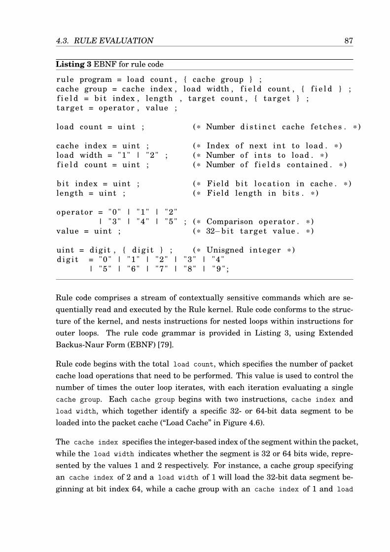
4.3. RULE EVALUATION 87
Listing 3 EBNF for rule code
rule program = load count , { cache group } ;cache group = cache index , load width , f i e l d count , { f i e l d } ;f i e l d = b i t index , length , target count , { target } ;target = operator , value ;
load count = uint ; (* Number d i s t i n c t cache fetches . * )
cache index = uint ; (* Index of next int to load . * )load width = "1" | "2" ; (* Number of ints to load . * )f i e l d count = uint ; (* Number of f i e l d s contained . * )
b i t index = uint ; (* Field b i t l ocat ion in cache . * )length = uint ; (* Field length in b i t s . * )
operator = "0" | "1" | "2"| "3" | "4" | "5" ; (* Comparison operator . * )
value = uint ; (* 32−b i t target value . * )
uint = dig i t , { d i g i t } ; (* Unisgned integer *)d i g i t = "0" | "1" | "2" | "3" | "4"
| "5" | "6" | "7" | "8" | " 9 " ;
Rule code comprises a stream of contextually sensitive commands which are se-quentially read and executed by the Rule kernel. Rule code conforms to the struc-ture of the kernel, and nests instructions for nested loops within instructions forouter loops. The rule code grammar is provided in Listing 3, using ExtendedBackus-Naur Form (EBNF) [79].
Rule code begins with the total load count, which specifies the number of packetcache load operations that need to be performed. This value is used to control thenumber of times the outer loop iterates, with each iteration evaluating a singlecache group. Each cache group begins with two instructions, cache index andload width, which together identify a specific 32- or 64-bit data segment to beloaded into the packet cache (“Load Cache” in Figure 4.6).
The cache index specifies the integer-based index of the segment within the packet,while the load width indicates whether the segment is 32 or 64 bits wide, repre-sented by the values 1 and 2 respectively. For instance, a cache group specifyingan cache index of 2 and a load width of 1 will load the 32-bit data segment be-ginning at bit index 64, while a cache group with an cache index of 1 and load

4.3. RULE EVALUATION 88
width of 2 will transfer the 64-bit data segment located at bit index 32 within thepacket. Following these values, field count specifies the number of distinct fieldscontained within the loaded cache group, and is used to control the number of it-erations performed in the intermediate loop. Each iteration of this nested loopextracts a specific field from the packet cache, and compares it to a set of targets.
Similar to cache group instructions, each field begins with two values, bit indexand length, which indicate the fields location and width respectively. The field’sbit index is defined to be relative to the start of the packet cache, in order toavoid having to calculate a cache-relative index at run-time. For example, a bitindex of 16 indicates that the field begins at bit 16 in the first integer in packetcache, while a bit index of 52 indicates that the field begins at bit 20 in the secondinteger. As packet cache is limited to 64 bits, and field lengths are limited to 32bits, it follows that:
∀ field∈cache group,
bit index< 64,
length≤ 32,
bit index+ length≤ 64.
Each field is extracted using a combination of bit-shifting and bit-masking (seeSection 4.3.4), represented in Figure 4.6 by the “Extract Field” box. Once a fieldhas been extracted, the target count is used to limit the innermost loop, whichcompares a single target to the previously extracted field value during each iter-ation. A target is comprised of an operator (represented by an integer between0 and 5) and a 32-bit value to compare to the extracted field. The operator valueis used in a non-divergent switch statement to select the appropriate comparisonto perform. After each evaluation, the boolean result is stored in global memoryusing the coalescing memory pattern introduced in Section 4.2.3.
In summary, each rule program defines one or more cache groups, each containingone or more fields, which in turn define one or more comparisons. Decomposing andreconstituting the high level GPF filter specification into these groups, orderingthem so as to minimise texture memory overhead, and grouping them so as toavoid redundant field extraction is the responsibility of the GPF compiler, and willbe discussed in Section 4.5.2.

4.3. RULE EVALUATION 89
Figure 4.7: Example extraction of a field spanning both cache integers.
4.3.4 Extracting Packet Data
Fields are extracted from the packet cache using bit-shifts, and is facilitated by aseparate device function. Detailed psuedocode for the extraction function is pro-vided in Listing 4. While the function employs decisional branching, individualthreads never diverge, as all branch comparisons operate on constant variablessupplied by the rule program. Furthermore, the packet cache has been mapped toprevent shared memory bank conflicts (see Section 3.4.5), by ensuring that adja-cent threads access adjacent cache indexes.
To extract a particular field from packet cache, the function first determines if thefield begins in the first cache integer or the second by testing to see if the index ofthe field is less than 32. If field_index≥ 32, then the field is entirely containedby the second cache integer and may be extracted. If the field starts in the first 32bits of packet cache, however, the function must determine whether the field spansmore than one integer, achieved by summing the field_index and field_width.If the sum is less than 33, then the field is entirely contained within the first cacheinteger, and may be extracted. If, however, the sum is greater than or equal to 33,then bits from both cache integers need to be combined into a single field.
To achieve this, the first integer in the packet cache is shifted left to remove all

90
Listing 4 Psuedocode for field extraction.
/ /PACKET_CACHE[ ] − shared memory cache/ / f i e ld_ index / f i e ld_ length − f i e l d information re la t i ve to
packet cache
unsigned int ans ;
i f ( f i e ld_ index < 32) / / s tart index i s in f i r s t cached integer{
ans = PACKET_CACHE[ threadIdx . x ] ;
/ / i f value contained in only the f i r s t int/ / − crop surrounding b i t s using s h i f t si f ( f i e ld_ length + f ie ld_ index < 33){
ans = ( ans << f ie ld_ index ) >> (32 − f i e ld_ length ) ;}
e l se / / value contained in two ints{
ans = ( ans << f ie ld_ index ) >> (32 − f i e ld_ length ) ;ans += PACKET_CACHE[256 + threadIdx . x ] >> (64 −
f i e ld_ index − f i e ld_ length ) ;}
}e l se / / s tart index i s in second cached integer{
ans = PACKET_CACHE[256 + threadIdx . x ] ;ans = ( ans << f ie ld_ index − 32) >> (32 − f i e ld_ length ) ;
}return ans ;

4.4. EVALUATING FILTERS 91
leading bits, and then shifted right by the difference between the fields lengthand the size of the register container. This positions the field such that it startsfield_length bits from the right-most bit in the register, with the bits correspond-ing to the portion of the field stored in the second cache integer containing onlyzeros. This value is stored in the extraction register. The portion of the field con-tained in the second cached integer is then shifted as far to the right as possibleand added to the value contained in the extraction register, which results in theextracted field value. An example of this extraction process for a field spanningboth cache integers is provided in Figure 4.7.
4.4 Evaluating Filters
Filter evaluation uses the results generated and stored in coalesced global memoryby the Rule kernel to classify each packet against every filter defined in the filterset. This ensures that all possible results are collected for each packet, and allowsfor divergence free classification by broadcasting identical instructions to all activethreads. An exhaustive approach such as this is, however, quite computationallyexpensive, particularly when processing large filter sets. To mitigate this, the filterevaluation mechanism uses a two stage classification process which allows commonsub-predicates to be reused.
This section motivates the filter evaluation process, and describes both the filtercode grammar, and how this code is interpreted within the executing kernels toproduce a complete set of classification results.
4.4.1 Predicate Evaluation
Evaluating predicates programmatically is often achieved through the use of a non-deterministic recursive decent parser [9], as these are relatively easy to implementby hand, and elegantly support arbitrary depth nested parenthesis. Recursivefunction calls, however, are only supported on Fermi devices [64], and are typicallyless efficient with regard to both speed and memory utilisation than comparable it-erative methods [84]. Instead, filter evaluation is facilitated by a three-tier nestedpredicate evaluation loop, depicted in Figure 4.8.

4.4. EVALUATING FILTERS 92
Figure 4.8: Iterative predicate evaluation.
Figure 4.9: Precedence hierarchy in parenthesis-free predicate evaluation.
This nested loop is structured to maintain the precedence relationships betweenthe logical conjunction (&&), logical disjunction (||) and logical inverse (!) operatorswithin a particular parenthesis-free predicate. Without parenthesis, these prece-dence relationships remain constant; ! has a higher precedence than &&, which inturn has higher precedence than ||. For instance, the logical predicate a || b && !c|| !a && c || !b has implicit parenthesis a ||( b && (!c)) || ((!a) && c) || (!b) . Fig-ure 4.9 illustrates the evaluation of this predicate using the iterative mechanismdepicted in Figure 4.8. The outer-most loop is ignored, given that only a singlepredicate is defined.
The OR row in Figure 4.9 corresponds to OR Element loop in Figure 4.8, which

4.4. EVALUATING FILTERS 93
would in this case iterate four times, each time evaluating a particular OR element.An OR element is a sub-predicate that does not itself contain an || operator. AnOR element contains one or more AND elements, each referencing a result storedin global memory, which may be inverted when the value is collected, if desired.The logical conjunction of the AND elements contained in an OR element is founditeratively, and used by the outer OR Element loop, which iteratively finds thedisjunction of all OR element results. Once a predicate is evaluated, its result isstored in global memory using the coalescing output format illustrated in Figure4.3.
While this provides a sufficiently accurate overview of the iterative predicate eval-uation process, it should be noted that actual Filter code is encoded differently inorder to improve execution efficiency (see Section 4.4.3).
4.4.2 Supporting Parenthesis
In order to support the evaluation of predicates containing parenthesis using theparenthesis-free evaluation mechanism depicted in Figure 4.8, Filter evaluationemploys an optional Subfilter kernel, which evaluates common predicates and sub-predicates, so that those results may be used during final classification. For in-stance, the predicate a && (b || c) may be evaluated by first calculating x = b ||c in the Subfilter kernel, and then finding a && x in the Filter kernel. The Subfil-ter kernel may be further applied to reduce redundancy, as any other filter whichcontains the predicate b || c may replace that operation with a reference to x.
Both the Subfilter and Filter kernels execute the same evaluation function, butstore results in different regions of global memory. The Subfilter uses the sameresults array as the Rule kernel, while the Filter kernel outputs results to a sep-arate classification results array. Like rule results, Subfilter results may be usedin other subfilters, as long as no circular references are defined. Filter results, onthe other hand, may not be used in other kernels. For example, the predicate !(a&& (b || c)) may be evaluated using the subfilters x = b || c and y = a && x, andthe filter !y.
As with Rule kernel architecture, this optimisation exploits the underlying redun-dancy found in typical filter sets (see Section 2.3.3), by effectively reducing theevaluation of a redundant multi-rule sub-predicate (involving more than one high-latency global memory read) into a single coalesced load operation.

4.4. EVALUATING FILTERS 94
Listing 5 EBNF for Filter and Subfilter Code
f i l t e r program = { f i l t e r } ;f i l t e r = or count , { or element } ;or element = and count , { and element } ;and element = not value , rule index ;
or count = unsigned integer ; (* No. o f elements to OR. *)and count = unsigned integer ; (* No. o f elements to AND. * )not value = "0" , "1" ; (* 1 i f NOT, 0 otherwise . * )rule index = unsigned integer ; (* Index of rule to load . * )
unsigned integer = dig i t , { d i g i t } ;d i g i t = "0" | "1" | "2" | "3" | "4"
| "5" | "6" | "7" | "8" | " 9 " ;
4.4.3 Filter Code
Filter code, contained in constant memory, encodes instructions which direct theexecution of the Filter and Subfilter kernels. Similarly to rule code, the grammarsyntax of filter code — shown using EBNF notation in Listing 5 — is designed toreduce the amount of processing performed by the kernels during each iteration. Afilter program contains one or more filter definitions, which are evaluated one at atime during each iteration of the outer Filter loop (see Figure 4.8). The number offilters defined in the filter set is stored separately in constant memory, and is usedto control the number of iterations performed in the outer loop.
Each filter begins with an or count, indicating the number of or elements thatneed to be evaluated, followed by one or more or element definitions. Similarly,each or element starts with an and count, specifying the number of and elementsthat it contains. The or count and and count values are used directly by theevaluation function to control the number of iterations performed by the OR loopand AND loop respectfully. Finally, each and element comprises a not value anda rule index, with the latter specifying the index of the value to be loaded fromrule memory, and the former indicating whether the value should be inverted ornot. Figure 4.10 illustrates this encoding scheme using the filter code for the pred-icate depicted in Figure 4.9.
To improve efficiency in the future, the OR evaluation loop may be adjusted to fa-cilitate logical short circuits. In the OR evaluation function, the evaluating loop

4.5. HIGH-LEVEL GRAMMAR 95
Figure 4.10: Filter code representation of the predicate in Figure 4.9.
short circuits to true if any of the OR elements returns a true value. Short circuitevaluation cannot be easily and efficiently implemented in the AND loop, as thiswould require thread synchronisation after each set of and elements is processedin order to avoid significant warp-level divergence potential in the surroundingOR loop. Unfortunately, any thread synchronisation performed within a divergentexecution path that only a subset of threads in a warp follow (which would beexpected in this case) will cause the kernel to either hang or malfunction [64]. Incontrast, when performing short circuit evaluation within the OR loop, a particularthread simply sleeps until all threads are ready to write results to global memory.As all filters will be evaluated, synchronisation can occur within the outer Filterloop, prior to this global memory write, without negatively affecting kernel execu-tion. Due to the SIMD nature of warp execution however (see Section 3.3.3), shortcircuited logic only provides a performance benefit if all threads in the executingwarp are short circuited, and is therefore only truly useful when evaluating longpredicates which match only a small subset of packets. It is therefore a relativelylow-priority optimisation.
4.5 High-Level Grammar
Rule and filter evaluation depend heavily on error-free kernel specific instructions— rule and filter code specifically — to direct packet classification. The grammarsused to encode these instructions are, however, relatively low-level with respect tokernel architecture, and are difficult to program by hand. To address this, ruleand filter code is compiled on the fly from a unified high-level filter specification

4.5. HIGH-LEVEL GRAMMAR 96
language, which abstracts away low-level technicalities to improve usability. Thissection details the syntax of this high-level grammar, and explains how GPF pro-grams written in this syntax are optimised and compiled into efficient rule andfilter code.
4.5.1 Grammar Syntax
Filter sets are specified using a relatively small Domain Specific Language (DSL),implemented in ANTLR v3 (ANother Tool for Language Recognition, Version 3)and C# 4. A DSL is a language which targets a specific problem or application do-main exclusively, and often supports specialised notation tailored for that domain[66]. The DSL uses the filter specification to generate a tree structure, which is op-timised and emitted as rule code and filter code for processing on the GPU device.For further information regarding DSLs and their implementation using ANTLR,the reader is directed to “The Definitive ANTLR Reference: Building Domain Spe-cific Languages” by Terence Parr.
The EBNF for the high-level filter classification grammar, called GPF code for sim-plicity, is provided in Listing 6.
GPF code allows for the specification of a variable number of filter and subfilterdeclarations, utilising a syntax similar to that of structs and classes in C style lan-guages. Filters are declared using the filter keyword, while sub filters are identi-fied using the sub keyword. Both filters and subfilters require a unique identifier,or label, which is included to allow for explicit reuse of the associated predicate inother predicates, and when returning the filter classification results to the user.Each filter and subfilter declaration concludes with a single predicate definition,contained in braces, using the standard C-style boolean operators, with expectedprecedence rules and full support for parenthesis.
Predicates may operate on both rule definitions, and id values referencing otherfilters and subfilters. A rule definition specifies the location and dimension of thefield to be evaluated, using the notation index : length, and the comparison to beperformed on it. Comparisons are specified using one of the six standard compar-ison operators, and a target value encoded as either an integer value, a hexadeci-mal value, or an IPv4 address. Subnets are included to provide a simple notationfor specifying comparisons on networks with non-standard sub-network division

97
Listing 6 EBNF for the GPF Grammar
program = declaration , { declarat ion } ;declarat ion = f i l t e r | sub f i l t e r ;
f i l t e r = f i l t e r , id , predicate ;sub f i l t e r = sub , id , predicate ;
predicate = { , or node , } " ;or node = and node , { || , and node } ;and node = not node , { &&, not node } ;not node = [ ! ] , atom ;atom = id | rule | sub predicate ;sub predicate = ( , or node , ) ;
rule = f i e ld , op , target ;f i e l d = integer , : , integer ;op = == | != | < | > | <= | >= ;target = integer | ip address | hex value ;
ip address = ip byte , " . " , ip byte , " . " , ip byte , " . " , ip byte ,[ " / " , integer ] ;
ip byte = integer | "*" ;
id = ( l e t t e r | caps | " _ " ) , { l e t t e r | caps | " _ " | d i g i t } ;integer = dig i t , { d i g i t } ;hex value = "0x " , hex , { hex } ;
d i g i t = "0" | "1" | "2" | "3" | "4"| "5" | "6" | "7" | "8" | " 9 " ;
l e t t e r = "a" | "b" | " c " | "d" | " e " | " f " | "g " | "h" | " i "| " j " | "k" | " l " | "m" | "n" | " o " | "p" | "q" | " r "| " s " | " t " | "u" | "v " | "w" | "x " | "y " | " z " ;
caps = "A" | "B" | "C" | "D" | "E" | "F" | "G" | "H" | " I "| "J" | "K" | "L" | "M" | "N" | "O" | "P" | "Q" | "R"| "S" | "T" | "U" | "V" | "W" | "X" | "Y" | "Z" ;
hex = d i g i t | "a" | "b" | " c " | "d" | " e " | " f "| "A" | "B" | "C" | "D" | "E" | "F" ;

4.5. HIGH-LEVEL GRAMMAR 98
Listing 7 Example high-level filter program classifying packets against two dis-tinct port ranges.
/ / IPv4 && (TCP || UDP)sub tcp_udp { 96:16 == 2048 && (184:8 == 6 || 184:8 == 17) }
f i l t e r srcport_big { tcp_udp && 272:16 >= 4000 }f i l t e r srcport_small { tcp_udp && 272:16 < 100 }
points, and are defined using the standard IPv4 Classless Inter-Domain Routing(CIDR) syntax [77].
Listing 7 shows an example GPF program, containing a subfilter and two filters.The subfilter evaluates to true if the packet is an IP packet which uses either theTCP or UDP protocols, while each filter passes if this subfilter evaluates to trueand certain source port requirements are met. As is evident, the GPF grammar isstill in early development, and currently depends on the filter set designer to knowthe exact bit-offsets and lengths of fields, as well as the exact target values theyare to be compared to. A remedy to this issue is provided in Section 4.8.3.
4.5.2 Compiling GPF Code
The GPF code compilation process involves several stages of evaluation, which ulti-mately yields the information necessary to emit rule and filter code. Firstly, lexicalanalysis is performed to convert the GPF code character stream into an equiva-lent stream of language specific tokens. This token stream is then parsed into anintermediate data structure known as an Abstract Syntax Tree (AST), which issubsequently walked by two different tree walkers, emitting rule code for the Rulekernel and filter code for the Subfilter and Filter kernels respectively. An overviewof this process is shown in Figure 4.11. As ANTLR handles lexical analysis, pars-ing, and the construction and modification of ASTs internally [66], this sectionfocuses on how the AST representation of the filter program is walked to producethe data structures necessary for code emission. How these data structures areused to emit rule and filter code is considered to Section 4.5.3.
The initial AST output by the parser is processed by the Rule Walker, a tree walkerwhich scans the AST for all rule declarations (see Listing 6). When the Rule

4.5. HIGH-LEVEL GRAMMAR 99
Figure 4.11: Overview of the GPF compilation process.
Walker locates a rule, it is passed to the Rule Set, which first ensures the ruledefinition is unique, by comparing it to all other rules contained within it. If therule is unique, it is added to the Rule Set, and is given a unique identifier. Therule in the AST is subsequently replaced by an AST node containing its corre-sponding identifier in the Rule Set. If, however, a rule is added to the Rule Setwhich has been previously defined, the Rule Set discards the rule, and replacesits definition in the AST with the unique identifier of the equivalent existing rulein the Rule Set.
Once the Rule Walker has completed its pass over the AST, and has replaced allrule definitions with their corresponding Rule Set identifiers, the Filter Walkerbegins construction on the Filter and Subfilter sets. The Filter Walker maintainsboth a Filter Set and a Subfilter Set, each responsible for emitting a filter program.The Filter Set and the Subfilter Set are instantiations of the same object class, andthus operate in the same way. Each filter and subfilter definition is convertedby the Filter Walker into an equivalent Filter Tree object, which is ultimately re-sponsible for emitting filter code.
As device-side filter evaluation does not support parenthesis, sub predicates mustbe converted into subfilters. To begin, the sub predicate is compared to all ac-cepted filters and subfilters, to see if an equivalent predicate has already beendefined. If no equivalent filter or subfilter is found to replace the sub predicate,it is converted into an anonymous subfilter; a subfilter with a hidden, computer-

4.5. HIGH-LEVEL GRAMMAR 100
generated id, which cannot be referenced within other predicates. Once con-verted, it is given a unique identifier, which then replaces its full definition inthe parent predicate. If, on the other hand, a matching filter or subfilter is found,then the sub predicate is replaced by a reference to that filter or subfilter instead.If the sub predicate matches an existing filter, then that filter is converted into ananonymous subfilter, and replaced in the Filter Set by a filter containing its uniqueidentifier in the Subfilter Set.
Once a filter or sub filter has been converted into Filter Tree object, it is checkedto ensure no other filters have been referenced as sub predicates. If one of its con-tained identifiers references a filter rather than a subfilter, then that filter is con-verted into an anonymous subfilter and added to the Subfilter Set, and replaced inthe Filter Set by a filter referencing its unique identifier.
At this point, the Rule Set, Subfilter Set and Filter Set contain all the relevantinformation needed to emit rule and filter code for each stage of classification.
4.5.3 Emitting Kernel Code
The process of emitting rule and filter code comprises three phases which are exe-cuted sequentially. The first phase, handled by the Rule Set, emits rule code for theRule kernel as an unsigned integer array in unmanaged memory. To convert theexisting rule records into rule code, the Rule Set first groups all rules by field value,and converts these groups into rules containing one field and multiple targets, suchthat each resultant rule contains a field value that is unique.
Rule fields are comprised of both a start index and a length, which together deter-mine if a particular field spans one or two cache integers in rule code (see Section4.3.3). Using their field information, rules are divided into two groups: those whichspan a single integer (narrow), and those which span two adjacent integers (wide).Consider a rule r1, containing a field which spans a single integer at index n. Be-cause r1 spans only a single integer, it may be placed into one of three possibleinteger cache groups. Specifically, it may be included in:
1. a narrow cache group which spans only the integer at index n.
2. a wide cache group which spans the integers at n− 1 and n.

4.6. PACKET COLLECTION AND BUFFERING 101
3. a wide cache group which spans the integers at n and n+ 1.
Now consider a rule r2, whose field spans two integers at index positions m andm + 1. By its definition, and in contrast to r1, r2 can only be contained in a singlecache group, which must span m and m + 1. These cache groups are thus createdfirst, with each containing at least one rule. The Rule Set then attempts to fit theremaining rules which span a single integer into the already existing groups, andonly creates a new cache group if this cannot be done.
Once all rules have been assigned to a cache group, the Rule Set checks if any ad-jacent narrow cache groups could be combined into a single wide cache group, inorder to reduce the number of distinct loads from texture memory in the Rule ker-nel. As a final optimisation, the Rule Set uses the set of cache groups to determinethe first and last referenced integers in every packet, and passes this informationto the packet collector to facilitate edge cropping (see Section 4.6.3). Each field’sstart index is adjusted to reflect the removal of the leading unused integers, afterwhich the set is finally condensed and emitted as an unmanaged unsigned integerarray.
The second phase of the code emission process is performed within the SubfilterSet, which uses the final order of the rules emitted in the first phase, as well asthe order of subfilter evaluation, to determine the rule result index locations corre-sponding to each unique Rule Set and Subfilter Set identifier. These result indexvalues replace their corresponding identifiers within each subfilter, following whichthe subfilter set is emitted as an unmanaged unsigned integer array. This processis repeated for the Filter Set in the third phase. Once all three phases are com-plete, the unsigned integer arrays are passed directly to the GPF host thread inpreparation for transfer to the CUDA device.
4.6 Packet Collection and Buffering
Before packets can be processed on the GPU, they must be collected from eitherlong term storage or a network interface, and stored in a buffer within host mem-ory. Currently, packet collection is facilitated by the WinPcap library, as it alreadycomprises all requisite packet collection functionality, and is well tested. Packetcollection is at present limited to dump file captures exclusively, as in contrast

4.6. PACKET COLLECTION AND BUFFERING 102
to transient live captures, the classification and performance results produced bydump files are verifiable and repeatable.
This section describes the design and implementation of the packet buffer, andsubsequently considers the bandwidth gap between host memory and long termstorage, and how this gap can be reduced.
4.6.1 Packet Buffering
Once collected from long term storage, packets must be stored in host memory be-fore being dispatched to the GPU for processing. While small dump files that donot exceed the available capacity in GPU DRAM can be processed in a single batch,larger packet sets must be divided into smaller batches and processed sequentially.These batches are stored temporarily within a circular buffer containing n packetbuckets, where n ≥ 1 is a user defined value. As all buffer buckets are stored inpage-locked host memory (see Section 3.5.1), the number of buckets, n, is limitedby the capacity of host memory, and should be kept small to ensure optimal perfor-mance.
The packet buffer executes in its own thread, collecting packet data concurrentlywith the execution of the main program thread. After the filter program has beencompiled and emitted (see Section 4.5), the main thread spawns the packet bufferthread, specifying the dump file to process, the size of each batch, and the totalnumber of buffers to use. The packet buffer also uses information collected duringthe compilation process to facilitate edge cropping (see Section 4.6.3).
During execution, each of the n buffer buckets is filled sequentially, until either allbuckets are full or the dump file is exhausted. When the filter program transfersa batch of packets from the packet buffer, it requests a lock on the least recentlyfilled packet bucket, which it acquires if or when the bucket is full. Once a lockis acquired on a buffer bucket, the filter program transfers all contained data todevice memory, bound to a texture reference. It then releases its lock on the bufferbucket prior to classification, which allows the bucket to be refilled during ruleand filter evaluation. In the unlikely event that the buffer thread fills all allocatedbuckets, it sleeps until a lock release is signaled by the program thread, after whichcontinues refilling the newly emptied buffer.

4.6. PACKET COLLECTION AND BUFFERING 103
Buffer configuration is designed to be flexible enough to facilitate a variety of us-age scenarios. Using large buffer buckets ensures fewer kernel invocations andfull GPU occupancy, providing the best per packet performance for offline dumpfiles, but requires millions of packets to be collected before classification can com-mence, resulting in increased latency. In contrast, by using a larger number ofmuch smaller buffers, packets may be dispatched to the GPU for classification morefrequently, providing lower latency between each iteration of classification.
The packet buffer is implemented in C#, while the filter is implemented in C++. Assuch, there is the potential for conflict between managed and unmanaged memorywhich would typically require an extra memory copy operation between the twomemory spaces to alleviate. This is avoided by declaring the buffers in unmanagedmemory, so that they can be passed, by reference, from the packet buffer directlyto the executing filter program. The buffers are initialised as page-locked, write-combined memory (see Section 3.5) within the filter program using the CUDA Run-time API, and are then passed by reference to the C# packet buffer to be managed.This memory is ultimately released by the filter program on termination.
The remainder of this section considers various means of improving the rate oftransfer to and from the packet buffer, with particular focus on overcoming thebandwidth gap between long term storage media and the host RAM.
4.6.2 Bandwidth Considerations
Before packet classification can commence, packet data must first be transferredbetween long term storage media and a buffer bucket in host memory, before ul-timately being copied from this bucket into device memory via the PCIE 2.0 bus.This indicates that the maximum speed at which a particular packet set can betransferred into device memory for processing is bounded by the rate at whichpackets can be read from long term storage. A bar graph showing the peak theo-retical bandwidths (using a logarithmic scale) of a typical 7200 RPM (RevolutionsPer Minute) Hard Disk Drive (HDD), the SATA II and III interfaces, the PCIE 2.0bus (upstream only), and DDR3 1600 SDRAM (Synchronous Dynamic RAM) is pro-vided in Figure 4.12. The figure shows that the maximum transfer rate supportedby the SATA III interface is over an order of magnitude slower than transfers be-tween the PCIE 2.0 bus and host memory. This causes a significant bottleneckin data transfer that is further exacerbated by the limited internal bandwidth of

4.6. PACKET COLLECTION AND BUFFERING 104
Figure 4.12: Peak theoretical transfer rate comparison.
HDD media, which falls far short of even the SATA II interface [71]. State-of-the-art Solid State Drives (SSDs), which are both more expensive and less commonthan HDDs, provide significantly better performance, but still fall short of the peaktransfer rates facilitated by the SATA III interface.
There are two primary ways to improve the transfer rate between long term storageand the PCIE 2.0 bus: stripe data over multiple physical drives, or employ a vir-tual drive residing in high bandwidth host RAM. Striping packet data over severaldrives can dramatically improve read times — as packet data can be transferredfrom multiple disks simultaneously — but requires a special storage configuration,and is expensive in terms of both hardware and energy consumption.
The second alternative is to partition an area of host RAM as a virtual disk, andtransfer packet data to this RAM disk prior to packet collection. RAM disks pro-vide bandwidth equivalent to host memory, and are therefore potentially fasterthan the combined throughput of all eight upstream channels of the PCIE 2.0 bus.Unfortunately, host memory is a scarce resource, and is generally not available inabundance. Furthermore, long term packet captures may span well over 10 giga-bytes of data, and it is for these packet sets that issues of performance are themost relevant. Finally, as RAM disks are partitioned in volatile memory, packetdata must be copied from non-volatile long term storage media prior to processing,which defeats the purpose of using a RAM disk if the dumpfile is only processed

4.6. PACKET COLLECTION AND BUFFERING 105
once.
Determining the best storage solution is thus subjective, as it largely depends onthe availability of system resources, the availability of specialised hardware, thesize of the dump file to be processed, and the number of times the dump file is ex-pected to be read. Luckily, the filter program is essentially agnostic to the mediumbeing used, and will accept any hardware supported by the operating system.
4.6.3 Packet Cropping
An important observation when considering the collection of packets is that mostof the packet data is never used by the filter program. Consider, for instance, afilter set identifying TCP/IP packets with various source address, source port anddestination port combinations, transported using the Ethernet II protocol. To iden-tify the packet as a TCP/IP packet, the 2-byte type field of the Ethernet II frameheader is compared to the hexadecimal value 0x800, while the 1-byte IP protocolheader field is compared to the value 0x08 to determine if the packet uses the TCPconnection protocol. The packets 4-byte source address, 2-byte source port and2-byte destination port header fields are also evaluated, such that packets whichpass all five tests are classified by the filter. In this example, only 11 bytes of dataper packet are actually used by the classifier, while the rest of the data is essen-tially ignored. As memory bandwidth between long term storage, host memory anddevice memory is a significant bottleneck, it is thus worthwhile to apply this obser-vation to reduce the amount of packet data collected from disk and transferred tothe device.
Achieving this programmatically is relatively simple. Once the user has definedthe filter set using the Domain Specific Language (DSL) defined in Section 4.5.1,the DSL compiler calculates which bytes in the packet header have been used inthe filter program, and which bytes can be ignored. From here, it is possible to ei-ther remove all unused bytes, or crop the unused bytes at the beginning and end ofthe packet. While removing all unused bytes would likely improve transfer speedsto some degree, this comes at the expense of increased processing demands anddisk I/O requests during collection. In contrast, as field comparisons typically tar-get a relatively small region of the header, edge cropping is effective at eliminatinga significant proportion of redundant transfer, without requiring multiple indepen-

4.6. PACKET COLLECTION AND BUFFERING 106
Figure 4.13: Example effects of edge cropping optimisation on packet size.
dent copy operations per packet. Figure 4.13 provides an example of the effects ofedge cropping for an arbitrary filter set.
Edge cropping provides an inexpensive means of both reducing per-packet transferoverhead, and increasing the number of packets that can be processed on a par-ticular device at one time. Edge cropping is not currently possible during packetcollection from long term storage, however, as it is not efficiently facilitated bythe WinPcap library. WinPcap and its limitations are discussed in the followingsection.
4.6.4 Parsing Packet Data
The GPF design currently utilises the WinPcap library to facilitate dump file pars-ing, largely for the sake of implementation simplicity. WinPcap is not, however,particularly efficient with regards to dump file processing. This is most easily il-lustrated when comparing between the parsing times of low and high bandwidthstorage media. Figure 4.14 shows the comparative parsing times of three packetcaptures (described in Section 5.1.3), read from both a 7200 RPM SATA II HDDand a DDR3 1600 RAM disk. Measurements were taken of both unfiltered andfiltered capture parsing, with the latter comprising three relatively simple filters.
With regard to the unfiltered test, as DDR3 1600 RAM provides just under 100xthe bandwidth of a SATA II HDD, one would expect to see a performance differ-ence of around two orders of magnitude between these mediums when no filter isapplied. Instead, timings for filtered and unfiltered traffic on both storage mediawere almost identical in Figures 4.14a and 4.14b, while in Figure 4.14c, the RAMdisk outperformed the SATA II HDD by up to only 13 percent. This indicates thatlimitations in performance are not the result of slow hardware transfer rate or poorfiltering performance, but the architecture of WinPcap itself.

107
(a) Packet set A - 183,617 packets, roughly 1KB each
(b) Packet set B - 2,445,815 packets, roughly 70B each
(c) Packet set C - 26,334,066 packets, roughly 70B each
Figure 4.14: Comparative WinPcap dumpfile filtering times for HDD vs. RAM disk.

4.7. ANALYSIS EXTENSIONS 108
GPF currently utilises WinPcap despite these limitations, as it is sufficient for thepurposes of measuring GPU classification performance. The WinPcap dump fileparser will be replaced by a more efficient custom solution better suited to the taskat a later stage. For now, however, it should be noted that the dump file parsingspeeds presented in the remainder of this thesis do not reflect an upper boundfor performance, and should improve significantly when a more efficient parser isused.
4.7 Analysis Extensions
While the primary components of GPF discussed thus far are sufficient to enablegeneral parallel packet classification, they lack features necessary to acceleratepacket analysis processes used in the calculation of metrics. These limitations areaddressed through extensions intended to supplement existing classification func-tionality with additional analytical and domain-specific kernels. Such extensionsprovide a mechanism to perform further calculations on both packet data and fil-tering results, in order to derive further information relating to the composition ofthe packet set.
This section introduces three relatively important extensions applicable to the do-main of packet analysis, which collectively demonstrate how the basic filteringfunctionality may be supplemented for domain specific purposes.
4.7.1 Aggregating Classifications
While the classification process is capable of collecting detailed filter results fromeach individual packet, it does not provide a mechanism to count these results ef-ficiently. As such, in order to determine the percentage of packets in the packet setwhich match a particular filter, the filter results must be counted in the sequen-tial host thread. This sequential step is potentially quite expensive, particularlywhen classifying against several filters, which motivates the need for a device sideclassification aggregation (or reduction) kernel.
The aggregation kernel is invoked after the core classification kernels complete,and operates on specific filter results stored in device memory. As these results

4.7. ANALYSIS EXTENSIONS 109
have been stored using a layout conducive to both coalescing and aggregation, thereis no need to employ texture references to improve access latency. Once complete,the aggregation kernel outputs an array of 32-bit unsigned integers, where eachindex element corresponds to a specific requested filter.
This kernel may be implemented efficiently by employing the methodologies pre-sented in the white paper “Optimising Parallel Reduction in CUDA” in the CUDASDK [32]. The interested reader is encouraged to consult the aforementioned whitepaper for implementation information.
4.7.2 Returning Packet Data
A common task in analysis involves determining the distribution of packets withregard to a particular field. For instance, one may wish to find the distributionof source or destination ports specified in captured IP traffic, in order to identifyirregularities in running services. Performing this analysis using an exhaustiveclassification mechanism is highly inefficient, as the core filtering kernels wouldhave to process a unique rule for each possible port value.
In order to address this problem, an extension may be incorporated to collect thedata in one or more arbitrary packet fields, and store these values, grouped first byfilter and then by field, in order to ensure coalescing. With this extension in place,it would be possible to process those field values either sequentially on the host,or within further extension kernels on the GPU, using the filter results to deter-mine which values should be processed. For best performance in GPU functions,however, packet data could instead be loaded directly from texture memory, with-out the need for an expensive intermediate data collection kernel. This requiresthat packet data persist beyond filter evaluation, which would prevent the earlyconcurrent packet data transfer discussed in Section 4.2.1. To allow for both GPUaccelerated post-processing of packet data and preemptive packet transfer, devicememory may be partitioned into a double buffer, allowing for packets to be trans-ferred into one bucket, while post-processing filters operate on data contained inthe other bucket.

4.8. FUTURE FUNCTIONALITY 110
4.7.3 Time-stamp Processing
Inter-Packet Arrival Time (IPAT) is a useful metric for diagnosing software config-uration issues and detecting security threats, such as packet floods. Determiningthe inter-packet arrival time for a particular protocol requires processing the times-tamps associated with the each of the classified packets; information contained inthe capture metadata, and not in the packet header itself. Timestamps also pro-vide necessary context to allow for temporal observations such as the time of day,week or year that certain network events occur, which may help in deriving theircause.
To facilitate time-stamp processing, extension kernels may use both filter resultsand time-stamp information to calculate the IPAT for specific protocols, or anyother useful metrics which may aid in analysing a packet set.
4.8 Future Functionality
This section considers additional functionality, not included in the design of GPF,which may increase the flexibility, efficiency and ease of use of the GPF classifier.These features will be considered and developed more thoroughly in future work,but are worth introducing briefly nonetheless.
4.8.1 Arbitrary Field Sizes
A significant limitation of the core filtering functionality, with regard to packetclassification, is the lack of native support for evaluating fields larger than 32-bitsin width. This limitation results from numerous factors, including the access la-tency limitations of global memory, the scarcity of on-chip multiprocessor memory,and the added complexity introduced in kernel execution (see Section 4.3.2). Thiseffectively prohibits the evaluation of rules targeting larger fields, such as 128-bitIPv6 addresses, and thus seems to limit the generality of filter architecture.
Overcoming this limitation is relatively simple, and may be achieved by breakingdown larger fields into multiple smaller fields during the compilation process. Forinstance, consider an arbitrary 128-bit IPv6 address. While the 32-bit limitation

4.8. FUTURE FUNCTIONALITY 111
Figure 4.15: Dividing a 128-bit IPv6 address field into multiple sub-fields.
on field sizes makes evaluating this 128-bit address value in a single operationimpossible, note that the address is equivalent to a combination of eight 16-bitfields, or alternatively, four 32-bit fields (see Figure 4.15). Thus, this address maybe evaluated by finding the disjunction of these sub-fields from within a subfilter.This principle applies to any arbitrary length field exceeding 32-bits, and may besupported with relative ease by extending the the compiler to identify such fields,and divide them appropriately prior to code emission.
4.8.2 Decision Based Filter Evaluation
In Section 3.7.1 it was noted that divergent approaches typically employed to fa-cilitate packet filtering do not perform well on GPUs, thereby motivating an al-ternative non-divergent decompositional approach which compares all packets toall rules and filters. However, some protocols and field values are not nearly ascommon as TCP/IP, and may only occur in a very small percentage of packets. Thisresults in redundant memory transactions and computation in warps where nopackets match a particular filter. In such cases, where only a small subset of pack-ets are expected to be applicable to a particular filter, support for decision basedevaluation becomes quite useful.
To facilitate this, the GPF DSL may be extended to include a C inspired decisionalmechanism, allowing a filter set designer to reduce the computational overheadfor classifications which are expected to only match a small fraction of packets.An example of a possible syntax is shown in Listing 8, although this has not beenformalised or finalised. The if statement takes a predicate as a conditional argu-ment, which determines whether the filters declared in the if-block are executed.

4.8. FUTURE FUNCTIONALITY 112
Listing 8 Example Decisional Execution
f i l t e r some_f i l ter { sub1 && sub3 }
i f ( some_f i l ter || sub2 ){
/ / = { ( some_f i l ter || sub2 ) && sub4 }f i l t e r some_other_f i l ter { sub4 }
}
If this initial test fails, the thread simply writes a false result. When the test doessucceed, any additional rule and subfilter evaluations exclusive to filters in theif-block are collected, after which the filter is evaluated.
In cases where very few packets match the condition, decisional evaluation canavoid a significant amount of redundant processing by allowing non-participantwarps to escape kernels early and begin processing new packets.
4.8.3 Protocol Definitions
To ease filter creation, the GPF DSL may be extended to allow for the declarationof arbitrary protocol definitions, which may be referenced by one or more filtersso as to avoid manually specifying field offsets and target values. Protocol defini-tions may specify field indexes and lengths, define target values, and declare anynecessary preconditions. A hypothetical example of a protocol definition in useis provided in Listing 9. In this example, the protocol field of the IP header is ac-cessed using dot notation, and compared to either a statically defined target withinthe fields definition, or to a manually defined value. Note that while TCP is a validtarget for the ip.proto field, it would not be valid for the ip.version field, or anyother field which did not explicitly define TCP as a possible target. In the case ofthe example filter, the results of both rules is predicated on the packet being an IPpacket, which is not explicitly tested. This is the purpose of preconditions, whichspecify the comparisons needed to determine if a packet employs the base protocolor not. These preconditions are incorporated into the filter implicitly, thus reducingfilter specification complexity.
The syntax for specifying protocols has yet to be defined, but should alleviate muchof the complexity associated with creating filters once implemented.

4.8. FUTURE FUNCTIONALITY 113
Listing 9 Hypothetical use of an IP protocol definition.
f i l t e r some_f i l ter { ip . proto == tcp || ip . proto == udp }
4.8.4 Variable Header Field Lengths
Thus far, all fields have been treated as having a preset constant length, whichallows for the specification of fields using static index and length values when de-scribing comparisons. However, many protocols — including IP and TCP — allowfor header lengths to vary, in order to facilitate rarely-used options in addition toexisting header fields when necessary [16, 77]. Such protocols typically specifythe length of a particular packet within a header field, which is used to determinewhere the protocol header ends, and thus where the next protocol begins. Cur-rently, catering for variable header field lengths requires the specification of rulescorresponding to each possible offset, which can be expensive if header lengthsare expected to vary by any significant amount. Because packets specifying vari-able length headers are uncommon [16], supporting them has been designated arelatively low priority. Mechanisms for incorporating this functionality have beenconsidered, however, and will be explored once the basic filtering mechanism hasbeen tested.
4.8.5 Instruction and Results Compression
Instruction and results compression is intended to improve memory efficiency inboth programs and results — as well as potentially reduce host-device transfertime — at the expense of additional kernel logic. These are considered separately,beginning with results compression.
Currently, results are stored in device memory as boolean values, and consume afull byte of memory each. This results in wasted storage space and transfer band-width, as each result could be encoded as a single bit without compromising accu-racy. By compressing up to 8 results for each processed packet into a single byteusing bit-shifting and boolean algebra, memory utilisation and transfer overheadmay be reduced by up to a factor of eight. While this introduces overhead whenboth loading and storing values, the added space efficiency allows more packets to

4.9. SUMMARY 114
be processed per batch, and significantly reduces the amount of data that has to betransferred from the device.
Program compression operates on a similar premise to that of results compres-sion, but is slightly more complex to employ. Note that while all program instruc-tions for all kernels are stored as 32-bit integers, allowing for target values up to32-bits in length, many instructions can be adequately described using far fewerbits. Program compression is intended to capitalise on this, and reduce multipleinstructions into a single 32-bit word where possible. Not all instructions can becompressed of course, and so implementing this compression will require an ad-justed program syntax and specialised classification kernels.
Compression of this kind is likely to cause measurable kernel slowdown, and thusshould be limited to cases where filter program size and complexity is significantenough to warrant its use.
4.9 Summary
This chapter described the design and implementation of GPF in some detail, be-ginning with an outline of the basic classification process and an overview of thesystem architecture in Section 4.1, and followed by details regarding specific com-ponents in subsequent sections.
The common architectural components of the CUDA classification kernels werepresented in Section 4.2. This section covered, among other topics, the coalescingmemory pattern used to store results, the method used by kernels to execute filterinstructions, and details on an efficient concurrent execution configuration whichmay be employed to improve overall efficiency. Sections 4.3 and 4.4 then detailedthe architecture of the rule evaluation and filter evaluation kernels respectively, in-cluding their respective instruction grammars and the strategies used to minimisememory overhead, divergence and redundancy.
Having considered how packets are actually classified by GPF, Section 4.5 intro-duced the high-level DSL used to specify filter sets, and how this language is com-piled and emitted as kernel specific instructions for rule and filter evaluation. Fol-lowing this, the architecture of the packet buffer was described in Section 4.6, inaddition to considerations regarding how to transfer packet data from long term

4.9. SUMMARY 115
storage into the buffer efficiently. Finally, extensions to facilitate domain specificfunctions, as well as future improvements to the flexibility, efficiency and ease ofuse of GPF, were discussed in Sections 4.7 and 4.8 respectively.
In Chapter 5, a prototype implementation of this design is tested, with a primaryfocus on the accuracy and performance of the the GPU classification mechanism.

5Evaluation and Testing
THIS chapter details the testing performed on the GPF prototype. In general,the testing focuses on overall performance and flexibility, as well as verify-ing that the results generated are an accurate reflection of the packet sets
being classified.
Section 5.1 provides an overview of the testing procedure. In particular, it de-tails the primary differences between the deign and prototype implementation, de-scribes the test system and testing parameters, and lists the packet captures usedas well as the filter programs measured.
Section 5.2 describes how filter compilation and classification were verified as pro-ducing accurate, meaningful output.
Section 5.3 considers the validity of timing results, by finding the mean and stan-dard deviation of results for a particular packet set and filter program over 100iterations.
Section 5.4 demonstrates how classification time for a particular filter program isaffected when the packet capture being processed is varied.
116

5.1. TESTING CONFIGURATION 117
Section 5.5 concludes testing by measuring how performance scales between filterprograms of varying complexity.
Section 5.6 contextualises the performance measurements collected by comparingthem to the performance of both WinPcap and Libtrace.
The chapter concludes with a summary in Section 5.7.
5.1 Testing Configuration
Testing was performed on a functional prototype of the design presented in Chap-ter 4. It includes the core rule and filter evaluation kernels, encapsulated within a64-bit C++ DLL, as well as a C# .NET management program, incorporating func-tional yet limited implementations of the packet buffer and compiler components.In most instances, functionality was deliberately deactivated in order to simplifyperformance testing. A brief list of the most significant limitations and differencesis provided below:
• The classification kernels only process a single batch of packets, but returnper packet rule and subfilter results in addition to filter results, to aid inresults verification. Processing multiple batches is essentially superfluous,as the same operations are performed, in an identical way, on each batch.Thus, processing multiple batches does not impact the GPU side functions,and therefore falls outside of testing scope.
• For simplicity, packet collection from long term storage is facilitated by Win-Pcap, which dramatically inflates buffering time (see Section 4.6.4). Further-more, because WinPcap copies the entire packet into its internal buffer au-tomatically, the transfer minimisation techniques introduced in Section 4.6.3cannot be employed when copying packets from long term storage. This isacceptable, as these limitations have no direct impact on the performance ofthe classification kernels.
• The packet buffer is executed by the host thread, and as such does not runconcurrently with the classification process. This ensures that concurrentthreads do not compete for system resources, and inadvertently skew results.
5.1. TESTING CONFIGURATION 118
• All kernels execute from within the same stream, and as such do not leverageconcurrent execution and transfer. This allows for each kernel to be discretelytimed, without the potential for interference or delay by other executing ker-nels, or the data transfer process.
• Short-circuit evaluation logic has been disabled during predicate evaluation,as its effectiveness is heavily dependent on packet arrival order, which maypotentially skew results. For instance, if very few packets in a particularcapture match a short-circuited filter, then the timing results may indicatea much shorter execution time than would typically be expected. Further-more, it is difficult to determine how the extra decisional overhead requiredby short-circuit evaluation impacts overall performance in the general andworst cases. By deactivating short-circuit evaluation, the performance re-sults provide a better indication of baseline performance, which may be usedat a later stage to evaluate the comparative effectiveness of the short-circuitmechanism.
• The parser does not yet accept IP addresses or hexadecimal numbers as targetvalues, and relies solely on integers as input.
Despite these adjustments and limitations, the prototype implementation remainsrelatively complete, and is capable of reading in packet dump files, generating filtercode and classifying packets at high speed.
5.1.1 Test System
Testing was performed on an Intel Core2 Quad Q9550 2.83GHz Windows 7 x64desktop PC, with 8 GB of DDR3 1600 RAM and several terabytes of 7200rpm SATAII storage, using four separate CUDA capable graphics cards. The cards usedin testing were: an MSI N9600GT T2D512 OC (9600 GT), a Gainward GTX275896MB (GTX 275), an MSI N465 GTX Twin Frozr II (GTX 465), and an MSIN480 GTX (GTX 480). All cards used unmodified 263.06 Geforce drivers, acquiredthrough the NVIDIA website. A comparative overview of the technical specifica-tions of these cards is given in Table 5.1.

5.1. TESTING CONFIGURATION 119
9600 GT GTX 275 GTX 465 GTX 480Full Name MSI Gainward MSI MSI
Model N9600GT GTX275 N465GTX N480GTXVersion T2D512 OC GS 896MB Twin Frozr II M2D15
Compute Capability 1.1 1.3 2.0 2.0CUDA Cores 64 240 352 480
Device Memory (MB) 512 896 1024 1536Memory Type GDDR3 GDDR3 GDDR5 GDDR5
Core Clock (MHz) 650 633 607 700Memory Bandwidth (GBps) 54.9 121.1 97.8 169.2
Table 5.1: Technical comparison of test graphics card specifications.
5.1.2 Recording Execution Times
To measure the performance of the various components of the GPF prototype, eachof the classifiers classification and supporting functions were timed independently.Components of the system implemented on the host, such as the packet bufferand compiler, were timed using a .NET timer object, which has a resolution of 1millisecond. In contrast, CUDA kernels and transfers were timed using CUDAevents, which have a resolution of roughly 0.5 microseconds [62, 63].
Timing results collected from the executing host thread include:
• Code Emission — The time taken to parse GPF code into data-structures, andcompile and emit kernel code from these data-structures.
• Initialisation — The time taken to initialise the classifier and its associatedCUDA context, and allocate memory.
• Buffering — The time taken to collect and buffer packets on the host usingWinPcap.
The higher resolution device-side execution times reported include:
• Transfer — The time taken to transfer packet data to the GPU device.
• Rule kernel — The time taken to execute the Rule kernel.
• Subfilter kernel — The time taken to execute the Subfilter kernel.
• Filter kernel — The time taken to execute the Filter kernel.
• Collection — The time taken to collect the filter results from the GPU device.

5.1. TESTING CONFIGURATION 120
Packet Set A B CTotal Packets 183,617 2,445,815 26,334,066
Used In Testing All All 10,000,000Average Packet Size 1036 bytes 69 bytes 70 bytes
File Size 184 MB 199 MB 2,157 MBDuration 20 minutes 1 month 11 months
Table 5.2: Packet sets used in testing.
5.1.3 Packet Sets
Testing was performed using three packet sets, referred to for simplicity as A, Band C, the details of which are summarised in Table 5.2.
• Packet set A was captured from a live network interface, and contains bothIPv4 and IPv6 packets. This packet set is the most representative of a livepacket stream, and is the only packet set tested which includes IPv6 packets.
• Packet set B contains packets collected from a network telescope over themonth of August, 2009. This packet capture does not include much payloaddata, and thus consumes comparable disk space to packet set A, despite con-taining over ten times as many packets. Despite their similarity in size, cap-ture B takes significantly longer to process than A.
• Packet set C contains packets collected from a network telescope between the1st of October 2009 and the 31st of August 2010. Due to its size, it was notpossible to load all 26 million packets onto any of the GPU devices tested.Thus, the batch size for this set has been limited to 10 million packets, anumber small enough to be able to fit onto all three devices for all but onetest.
5.1.4 Filter Programs
The GPF prototype has been tested using six different filter programs of varyingcomplexity. The specifications for these programs are contained in Appendix A.For the purposes of testing, filters are categorised as being either simple filters orcompound filters. A simple filter is a filter which only references a single rule, andthus does not contain any predicate logic in emitted filter code. A compound filter

5.1. TESTING CONFIGURATION 121
is any filter which is not a simple filter. In reality, simple filters are not particularlyuseful and would rarely be employed except in the most trivial of cases, but theyare nonetheless useful when benchmarking performance.
The filter programs used to test the prototype classification kernels are describedbriefly below.
• IP Protocols (IPP) — This filter program is used exclusively in Sections 5.3and 5.4, and classifies packets against two subfilters and five filters. Thesubfilters test the type field in the Ethernet frame header, to identify anyIPv4 or IPv6 packets. Subsequently, this program identify all TCP packets(IPv4 or IPv6), UDP packets (IPv4 or IPv6), ICMP packets (IPv4), ICMPv6packets (IPv6), and ARP packets.
• Single Simple Filter (SSF) — The SSF program classifies all packets againsta single simple filter, comprising only a single rule, which tests if an Ether-net packet uses the IP protocol. This filter set is used to measure best caseperformance of classification.
• Multiple Simple Filters (MSF) — Expanding on SSF, the MSF program com-prises four filters, each containing a single rule that targets a unique field.These fields are: the Ethernet header type field, the IP header version andprotocol fields, and the TCP header source port field. This filter programwould not be particularly useful in a real world scenario, as testing for theTCP source port of a packet which is not guaranteed to be a TCP packet — ortesting for the IP version of a packet which is not an IP packet — may resultin false positives.
• Single Compound Filter (SCF) — The SCF program specifies a single multi-rule filter, which tests for TCP/IPv4 packets with a source or destination portgreater than or equal to 4000. This filter predicate is the first listed to employan anonymous subfilter.
• Multiple Compound Filters (MCF) — The MCF program defines three sub-filters and four filters, which collectively find all TCP/IPv4 packets with: asource port less than 150 or greater than or equal to 5000, a destination portless than 150 or greater than or equal to 5000, both source and destinationports less than 150 or greater than or equal to 5000, and both source anddestination ports greater than or equal to 150 and less than 5000. It employsboth named and anonymous subfilters, as well as all logical operators.

5.2. VERIFICATION 122
• Large Simple Filter (LSF) — the LSF program defines 60 simple filters, ofwhich half target 8-bit fields and half target 16-bit fields. Each filter containsa unique field, eliminating the possibility of rule reuse, although the 8 and 16bit filters operate on the same packet data (the 8 bit filters together target thefirst 30 bytes of each packet, while the 16 bit filters target the first 31 bytes).This filter set represents a relative worst case, as it is much larger than anyother filter set, and provides little opportunity for optimisation.
5.2 Verification
Verification was performed concurrently with performance evaluation, facilitatedby the network protocol analysis application WireShark (version 1.4.3). Test re-sults were verified through inspection of both the kernel instruction inputs, andthe per packet boolean results produced by the Rule, Subfilter and Filter kernels.This section details how this inspection was performed, and motivates why thismethod of verification is sufficient for the purposes of this testing.
5.2.1 Code Emission
Verification of the code emitter involves comparing the high-level GPF code to emit-ted kernel code, in order to ensure equivalence. This procedure may be brokendown into three steps:
1. The rule programs were inspected to ensure that all rules were defined,grouped and sorted correctly, and that each rule contained a single uniquefield value followed by one or more operator/targets pairs. Once verified, thecorresponding indexes of each rule in the rule output array were determined,to aid in predicate verification. As rule indexes correspond to the position ofthe rule in the kernel program (i.e. the result of the nth rule is stored in indexposition n− 1), this was a relatively straight forward process.
2. The subfilter programs (if defined) were inspected to ensure that all subfiltershad been detected and included, that all subfilter predicates were encodedcorrectly, and that the indexes contained in the subfilter predicates map to

5.2. VERIFICATION 123
the correct rule result indexes calculated in the previous step. Once com-plete, the corresponding rule results index associated with each subfilter wascalculated, using the same method as in the previous step.
3. Finally, the filter programs were inspected for correctness, and their con-tained predicates checked to ensure they reference the correct rule and sub-filter indexes calculated in steps 1 and 2.
5.2.2 Classifier Outputs
In addition to the per packet results output at the culmination of classification,the GPF prototype returns both rule and subfilter results, so that they may beinspected as well. These results are written to a text file, grouped by kernel, andthen by each individual rule, subfilter or filter.
For instance, consider a rule program comprising r distinct comparisons, to be ap-plied to a batch of p packets. The output produced by the Rule kernel is a booleanarray, containing r sets of p contiguous results. The results for the first, secondand last rules are stored in indexes 0 : (p − 1), p : (2p − 1), and (r − 1)p : (rp − 1)
respectively. Filter and subfilter results are stored similarly, although as subfilterresults are stored after rule results in the same boolean array, the first index ofthe first subfilter must be adjusted to point to the end of the rule results, rp, ratherthan 0. Thus, the first set of p subfilter results are stored in the rule index locationsrp : (rp+ 2p− 1). These sets of p results are summed on the host, to determine thenumber of packets in the batch which match each specific rule, subfilter and filter.
Outputs are verified in two stages:
1. For each rule, subfilter and filter, the total number of matching packets iscalculated on the host and compared to the number of packets returned byWireShark for the same comparison. This provides a strong initial indicationof results accuracy.
2. Next, results are inspected to ensure that they are stored at the correct in-dexes. To do this, the pattern of ones and zeros generated by each rule, subfil-ter and filter are compared to the filtered packet list in WireShark, to ensurethat they match. As it would be extremely time consuming to check every

5.2. VERIFICATION 124
packet in each set against every rule, subfilter and filter evaluated, only thefirst 1024 packets — and a random selection of result groups at later indexesin the packet set — were inspected in each test. Inspection was explicitly per-formed on one iteration of each test case, while subsequent iterations werechecked by comparing the resultant classification counts to those generatedby the first iteration.
With regard to the first stage of verification, note that some naive filters produceslightly different results to WireShark for certain packet sets. As an example,consider the TCP protocol. In IPv4, the 8-bit TCP protocol flag is located at bitindex 184, while in IPv6 this flag is located at bit index 160. In WireShark, theexpression ip.proto == 6 returns all the TCP packets from both IPv4 and IPv6.In most of the filters tested, however, rules relating to TCP reference the bit index184, which not only means all IPv6 TCP classifications are missed (false negatives),but also that some non-TCP packets may mistakenly be accepted due to correlatingvalues at bit index 184 in the IPv6 packet. Thus, this rule is only meaningful whencombined with other rules, which differentiate between IPv4 and IPv6 packets, ina single filter. The IP Protocols filter program provides a good example of this (seeAppendix A.1). In such instances, when a particular result differs from WireShark,verification was primarily supported by inspection of rule results and actual packetdata.
5.2.3 Validity of Verification Results
This form of verification is justified by a simple statistical observation, which shallbe discussed briefly. Consider a set of p packets, which is to be compared againsta single filter comprising a single rule. Suppose that, when classified by GPF, thenumber of packets in p which match the filter is identical to the number producedby a verified system such as WireShark. In this instance, if p is even remotelylarge, the probability that GPF will classify the correct number of packets, whilesimultaneously classifying packets incorrectly is extremely low. This probabilityshrinks further when several different, somewhat complex filter sets are processedagainst multiple packet traces with the same outcome. When multiple subsets ofper-packet results are individually verified, the probability that some classifica-tions are wrong becomes effectively negligible.

5.3. TIMING RESULTS VALIDATION 125
Put differently, for the classifier to pass these verification mechanisms and simulta-neously produce inaccurate classifications, it would have to classify the inspectedpacket results correctly, while producing the same number of false positives andfalse negatives in unobserved result indexes, over multiple filter programs andpacket sets. The probability of this occurring is minimal, making this simple veri-fication mechanism highly effective.
5.3 Timing Results Validation
Performance testing was validated by providing a measure of results variance forthe IP Protocols (IPP) program (see Section 5.1.4) over packet capture C (see Sec-tion 5.1.3). The number of packets processed was varied between one thousand,one million, and ten million packets, in order to evaluate variance under low, mod-erate and high load conditions. These three tests were repeated on each of the fourGPU devices. Tests were executed in batches of 20 at a time, after which the sys-tem was rebooted and the process repeated, so as to allow for comparison betweenuncached (cold) and cached (warm) classifications.
The IPP program classifies TCP, UDP and ICMP packets encapsulated in both IPv4and IPv6, as well as ARP packets, by evaluating three field values: the Ethernetprotocol’s type field, and the protocol field for both IPv4 and IPv6 packets. Notethat the subfilter declarations used here are not optimal for the current prototypesystem, and introduce a measure of redundancy. As both subfilters are simple fil-ters, containing only a single comparison, the classifier is forced to load the resultsof these rules into the Subfilter kernel and then restore them unchanged at an-other index in rule result memory. This could easily be avoided by updating thecode emitter to search for and eliminate such simple subfilters, and replacing theirreferences in other filters with the rule results index they contained. This will beaddressed in the next development iteration.
The remainder of this section presents the arithmetic mean and standard deviationof these results, concluding with a break down of the comparative performancebetween GPUs.

5.3. TIMING RESULTS VALIDATION 126
5.3.1 Mean Execution Time
The arithmetic mean of execution times for 103, 106 and 107 packets are shown inline graph form in Figure 5.1.
With respect to classification kernel times, the relative performance differencesbetween devices remains consistent across Figures 5.1b and 5.1c. This relationshipis not easily identified in Figure 5.1a, although a small performance boost is visiblebetween compute capability 1.3 and 2.0 device architectures. The remainder ofthe components, with the exception of the WinPcap buffer, showed no significantperformance differences across platforms, which is expected.
These results demonstrate that, for large packet sets and similar filter programs,the classification kernels can perform between one and two orders of magnitudefaster than the packet buffer, depending on the device they are executed on. Thus,with a more efficient capture loading function, this method of classification appearsviable.
5.3.2 Standard Deviation
The standard deviation (σ) of the timing results provides a measure of the degree towhich results varied from the mean value across all 100 iterations. The standarddeviation for each of these tests in provided as both an absolute value in Figure5.2, and as a percentage of the mean value in Figure 5.3.
The standard deviations of the timing results collected show that while host sidefunctions were prone to variance, the same was not true for kernel functions. Forinstance, whilst the percentage standard deviation of kernel functions was near100% in Figure 5.3a, the absolute values in Figure 5.2a show that this is due tothe mean value being extremely low (less than 0.05 ms), which ensures that evenextremely short time intervals register as significant. As the packet sets grow insize, however, the absolute standard deviation remains small whilst the packetcount, and thus the mean execution time, increases exponentially. This results inthe standard deviation to mean ratio dropping to around 0.1%.
While the mean execution time is exponentially higher in the larger packet sets, itdoes not reach a particularly high value, thereby inflating the significance of small

127
(a) 103 Packets
(b) 106 Packets
(c) 107 Packets
Figure 5.1: Mean completion time of the IP Filter program.

128
(a) 103 Packets
(b) 106 Packets
(c) 107 Packets
Figure 5.2: Absolute σ of performance validation tests, in milliseconds.

129
(a) 103 Packets
(b) 106 Packets
(c) 107 Packets
Figure 5.3: Relative σ of performance validation tests, as a percentage of the mean.

130
(a) 9600 GT
(b) GTX 275
(c) GTX 465
(d) GTX 480
Figure 5.4: Host component timing results for 107 packets over 100 iterations.

131
(a) 9600 GT
(b) GTX 275
(c) GTX 465
(d) GTX 480
Figure 5.5: CUDA component timing results for 107 packets over 100 iterations.

5.3. TIMING RESULTS VALIDATION 132
errors in comparison to host functions. Figures 5.4 and 5.5 plot the timing resultsfor 107 packets, for host and device related functions respectively. These plots pro-vide several important observations. Firstly, the classification kernels returnedrelatively uniform timings across all four devices, even during periods where hostside performance was severely impoverished. This, along with the low standarddeviations collected, show that performance of the classification kernels does notdiffer significantly between iterations.
In contrast, transfer and collection processes were severely affected by periods ofpoor performance on the host (indicated by arrows 1 and 2 in the figures). Arrow1 points out artifacts that appear in the first iteration after a fresh reboot, whichmay be the result of packet files being uncached, or due to other start-up processescompeting for resources. While these artifacts are relatively common in the hostside timings presented in Figure 5.4, CUDA related timings shown in Figure 5.5seem largely unaffected (although a slight degradation of transfer performance isvisible in Figure 5.5d). Arrow 2 points out regions of sustained poor performance,which occurred over two of the twenty reboot cycles. This slow down was likelycaused by one or more background processes on the operating system, and seemsto have reduced effective memory bandwidth, as only the packet buffer and thetransfer processes seem to be affected.
The standard deviation results indicate that the classification kernels perform con-sistently over many iterations and system reboots, while host-side execution andtransfers between the host and the GPU device are sometimes slowed by both ex-ecuting background services and uncached disk access. The level of consistencybetween kernel execution times is useful, as it indicates that even a single timingresult provides a good approximation of average processing time for that filter.
5.3.3 Performance Breakdown
Figure 5.6 contains a set of bar graphs, showing the proportion of time spent per-forming particular operations when classifying 107 packets on each GPU. Theseillustrate that buffering accounted for the majority of processing time, despite rep-resenting the collective time for only a single function. For instance, on the GTX480, the amount of time taken to buffer packets was roughly 85 times longer thanthe combined processing time for all three classification kernels. While bufferingthroughput may be improved significantly by implementing an optimised packet

5.4. PACKET THROUGHPUT 133
reader, this reader cannot exceed the bandwidth of the storage medium beingutilised, and thus will likely not be able to reduce collection times enough to fullyeliminate this bottleneck.
Compilation and initialisation components only execute once per classification,while buffering, transfer and collection, and kernel classification may be cycledcontinuously until all packets have been processed. Since packet buffering, PCIEtransfer and classification may all occur concurrently, the throughput of the clas-sification process is effectively bounded by the speed of the slowest component.This implies that the GPF classification kernels are capable of classifying packetsagainst this filter program faster than they can be collected from storage. This isunlikely to change, even if a specialised packet parser is employed.
5.4 Packet Throughput
In order to determine the throughput of the classifier with respect to packet count,the IPP program was used to classify packet batch sizes ranging, in increments of1,000 packets, from 1,000 to either: 183,000 (packet set A), 2,445,000 (packet setB) and 10,000,000 (packet set C). As these tests were extremely time consuming,throughput was only measured on the GTX 275 and GTX 480.
While validation testing was performed over multiple fresh system reboots andminimal background activity, throughput testing was performed in a typical liveenvironment, with a range of active competing processes. In addition, some of theseprocesses — such as the Internet Explorer 9 browser and Media Player Classic:Home Cinema — offload processing to the GPU to improve performance, and thuswere in direct competition with the GPF classification kernels. These results thusprovide a good indication of real-world performance on typical desktops, and helpillustrate how external load affects processing time.
Figure 5.7 shows two scatter plots of classification time against packet count forall three packet sets, performed on the GTX 275 and GTX 480 respectively. In thiscase, classification time has been calculated as the sum of the rule, subfilter andFilter kernels execution time, and does not include host side components, transfer,or collection.

134
Figure 5.6: Percentage of processing time spent performing component functions.
• Compilat ion & Init iali sa t ion • Bufferi ng • Class ificat ion Kern els • Transfer & Co llec t ion
9600GT
0.30%
GTX 275
0.3 1%
GTX465
GTX480
0.33%
0% 10% 20% 30% 40% 50% 60% 70% 80% 90% 100%

135
(a) GTX 275
(b) GTX 480
Figure 5.7: Execution time against packet count for all three packet sets.

5.4. PACKET THROUGHPUT 136
These scatter plots demonstrate a linear relationship between the number of pack-ets being processed and the time taken to perform classification, seemingly inde-pendent of the underlying packet set. This is expected, as all packets are croppedto the same size before transfer to the device, and are all subsequently evaluatedagainst the same classification instructions.
An anomaly, indicated by arrow 1 in Figure 5.7a, however, appears to challengethis conclusion, due to a very noticeable increase in classification time near the5,000,000 packet mark. At this point during testing, the GTX 275 being used tem-porarily stopped functioning, and had to be replaced with an equivalent card. Theactual performance of the new card (an MSI N275GTX TwinFrozr) differed slightlyfrom that of the original Gainward card, resulting in this artifact. As throughputtesting was performed after all other tests, this hardware failure did not affect anyother results. This anomaly is interesting, as it demonstrates that performancemay differ between different physical cards of otherwise equivalent architecture.
Another interesting anomaly is the apparent variance of results — particularly forlarger packet counts, and most notably in Figure 5.7b — which were not evidentduring performance validation testing. As the GTX 480 was acting as the primarydisplay card, and was thus under external load during testing, its variance wasslightly greater than that of the GTX 275. For instance, the slight slowdown no-ticeable between packet counts 6,000,000 and 7,000,000 on the GTX 480 graph,indicated by arrow 2, occurred while simultaneously performing GPU acceleratedHD video rendering in Media Player Classic - Home Cinema. This indicates thatwhile performance is certainly affected by external GPU load to some degree, over-all throughput is not significantly impaired. This is beneficial, as it implies theclassifier can execute efficiently as a background process, without negatively af-fecting the usability of the host, or the experience of the system’s user.
5.4.1 Linear Regression
Given evidence of a strong linear correlation between packet set size and process-ing time in the collected results, simple least squares regression has been used toderive a function td(x) = mx+ c, which is used to predict, for a given filter program,the time to classify a packet set td(x) on device d using only the packet count x,within some predetermined confidence level.

5.4. PACKET THROUGHPUT 137
Regression lines for both the validation and throughput results were calculatedand analysed using the Microsoft Excel function LINEST(), which uses the leastsquares regression method [2]. The standard errors for both m and c were also cal-culated, as well as the R2 and F statistics for each regression, for use in assessinghow well the regression lines fit the input data, and the likelihood that this fit isstatistically significant and not coincidental. A brief description of the statisticsgathered is provided below:
• The R2 statistic, or coefficient of determination, was used to measure howaccurately the regression models predict future outcomes [27, 70]. An R2
value of 1 indicates that the model perfectly fits the data set, while an R2
value of 0 indicates that the model does not fit the data at all. The R2 statisticwas produced by the LINEST() function.
• The F statistic was used to determine the probability that the correlation im-plied by the R2 statistic above occurred by chance exc [2], Freund and Wilson[27], Remington and Schork [70]. The FDIST() Excel function was used tofind this probability, using the F statistic and degrees of freedom output bythe LINEST() function [2]. The resultant F probability is a value between 0and 1, where 1 indicates that correlation implied by by the coefficient of de-termination is entirely coincidental, while an F probability of 0 indicates thatit is not coincidental at all.
• The t-Statistic was used to verify that the slope coefficient m is useful in esti-mating future classification performance [1, 2]. This was calculated by divid-ing the slope coefficientm by the estimated standard error form (both outputsof the LINEST() function), and comparing the absolute value of the result tothe tcritical value generated using the TINV() function, using a confidence in-terval of 99% (α = 0.01). If the absolute value of the result is greater thantcritical, then according to the t-test, the coefficient m is statistically significantin predicting td(x) [1, 2].
Each regression was performed using the performance results collected from allthree packet sets. Thus, each of the four regressions performed on validation timesincluded 300 elements, while the two regressions performed on the throughputtimes included 12,628 elements. The results of regression analysis are provided inTable 5.3.

5.4. PACKET THROUGHPUT 138
R2 F Probability t-test m error c error9600 GT 0.999991 0 Passed 2× 10⁻⁸ 0.116349GTX 275 0.999995 0 Passed 4× 10⁻⁹ 0.024165GTX 465 0.999998 0 Passed 1× 10⁻⁹ 0.00849GTX 480 0.999998 0 Passed 1× 10⁻⁹ 0.004675
(a) Validation Regression
R2 F Probability t-test m error c errorGTX 275 0.99975 0 Passed 5× 10⁻⁹ 0.025156GTX 480 0.999675 0 Passed 4× 10⁻⁹ 0.015148
(b) Throughput Regression
Table 5.3: Results of regression analysis
The high R2 statistics captured, in combination with the results of both the F -testsand t-tests performed, indicate that given a specific filter program and packet set,the time taken to process an arbitrary number of packets is a function of the packetcount, within a 99% confidence interval. Note, however, that the results in Figure5.3a are slightly higher than those in Figure 5.3b, while the m error is lower. Thisis likely a product of the increased results variance of the throughput tests, whichunlike the validation tests, had to compete with other running processes for systemresources.
5.4.2 Estimating Throughput
The calculated regression coefficients for the IPP program were used to predict theclassification packet throughput (packets/time), as well as the data rate (Gbps) forcaptures with three different average packet sizes (70 bytes, 300 bytes and 1024bytes). This information is provided in Table 5.4.
These results are extremely promising, showing significant improvement over bothWinPcap and Libtrace results (see Section 5.6), despite classifying a more complexfilter program and producing multiple results. These results, however, only reflectthe captured times for one specific filter set. In the following section, classificationperformance is measured over a range of different filter sets, in order to evaluatehow classification performance scales with respect to filter complexity.

5.5. FILTER PROGRAM PERFORMANCE 139
Packets / sec Packets / hour Gbps(millions) (billions) 70 B 300 B 1 KB
9600 GT 8.5 30.6 4 19 65GTX 275 29.9 107.7 16 67 228GTX 465 62.1 223.5 32 139 474GTX 480 98.3 353.9 51 220 750
(a) Validation Results
Packets / sec Packets / hour Gbps(millions) (billions) 70 B 300 B 1 KB
GTX 275 29 104.3 15 65 221GTX 480 97.2 349.5 51 217 741
(b) Throughput Results
Table 5.4: Projected packets per hour and filtering rates for varying average packetsize.
5.5 Filter Program Performance
This section shows the performance for different filter programs of varying com-plexity. Results are presented for five increasingly complex programs, descriptionsfor which are included in Section 5.1.4.
5.5.1 Single Simple Filter (SSF)
The SSF program (see Section 5.1.4) is the most basic of all filter sets evaluated,and simply tests each Ethernet protocol’s type flag to distinguish IP packets. Itdoes not require subfilter evaluation, and as such, subfilter timings have beenomitted from results. The timing results for all three packet sets are shown inFigure 5.8, given in milliseconds using a logarithmic scale.
Results are fairly consistent across packet sets, showing roughly equivalent ordersof magnitude difference in processing throughput for classification functions be-tween GPUs, for all packet set sizes. While device functions, code emission andinitialisation perform in a consistent manner across all sets, however, Figure 5.8bshows a slowdown of over two orders of magnitude for the 9600 GT during thebuffering phase of execution. This anomaly is almost certainly due to disk I/O orhost side thread conflicts outside of the control of the program. With regard toclassification kernel performance, the results indicate that the Rule kernel takes

140
(a) Packet set A
(b) Packet set B
(c) Packet set C
Figure 5.8: Single Simple Filter (SSF) program performance.

5.5. FILTER PROGRAM PERFORMANCE 141
Packets / sec Packets / hour Gbps(millions) (billions) 70 B 300 B 1 KB
9600 GT 37.3 134.2 19 83 284GTX 275 121.6 437.6 63 272 927GTX 465 264.1 950.9 138 590 2,015GTX 480 438.7 1,579.5 229 981 3,347
Table 5.5: Predicted Single Simple Filter (SSF) throughput and resultant data ratefor varying packet size.
longer to complete than the filter program. This is expected, as the Rule kernelmust load packet data from texture memory, crop the data correctly to determinethe value of the field, and then compare this value to a target. In contrast, the Fil-ter kernel only needs to transcribe a single rule value into the filter output array.
It was made evident in Sections 5.3 and 5.4 that the classification kernels performrelatively consistently, with minimal variance between times over multiple testiterations. As such, it is possible to derive a rough estimate of packet throughputusing the Sum of Least Squares regression method. This throughput may then beused to predict the bit rate achievable for three packet sets with differing averagepacket sizes. This information is presented in Table 5.5.
5.5.2 Multiple Simple Filters (MSF)
The MSF program extends the SSF program by adding three more simple filters(see Section 5.1.4). As with the SSF program, no subfilter results are reported forthis filter set. Results for this filter program are given in Figure 5.9.
With regard to performance results in Figure 5.9a, a slight slowdown is noticeablefor the 9600 GT during collection. This inconsistency is likely the product of theoperating systems overhead, as the instruction to transfer between the host andthe device occurs after the CUDA timer is started. As such, if the transfer operationis not serviced by the host thread immediately after the CUDA timer is started,or the bandwidth of system memory is exhausted by another process, the timingresults collected can be artificially inflated. Estimates of packet throughput anddata rates for each GPU when evaluating the MSF program are provided in Table5.6a.

142
(a) Packet set A
(b) Packet set B
(c) Packet set C
Figure 5.9: Multiple Simple Filter (MSF) program performance.

5.5. FILTER PROGRAM PERFORMANCE 143
Packets / sec Packets / hour Gbps(millions) (billions) 70 B 300 B 1 KB
9600 GT 10.7 38.6 6 24 82GTX 275 31.7 114.1 17 71 242GTX 465 71.2 256.2 37 159 543GTX 480 119.4 429.9 62 267 911(a) Predicted throughput and resultant data rate for varying packet size.
9600 GT GTX 275 GTX 465 GTX 480SSF Rule (ms) 170 57 30 17MSF Rule (ms) 549 216 107 62Rule Multiplier 3.5x 3.8x 3.7x 3.6xSSF Filter (ms) 99 26 9 6MSF Filter (ms) 348 100 34 22Filter Multiplier 3.5x 3.9x 3.8x 3.8x
(b) Comparison against Single Simple Filter processing times over capture C.
Table 5.6: Multiple Single Filters (MSF) program performance measurements andcomparison.
Thus, the MSF result set looks similar to that of the SSF program, with comparablehost timings and overhead related anomalies, and a similar relationship apparentbetween the tested GPUs regarding kernel processing times. There is, however, anoticeable difference in classification performance between this program and theSSF program. One might expect that, since the MSF program performs four timesas many comparisons as the SSF program, timings would be roughly four timesgreater. A comparison of results shows, however, that both kernels in the MSFprogram consistently took less than four times as long to complete (see Table 5.6b),indicating that the classifier scales well. Furthermore, the speedup associated withthe Rule kernel was slightly greater than that of the Filter kernel. This is likelydue to the caching mechanism, as the first two rules specified fall within the same32-bit cache block, which reduces the number of texture loads per packet duringrule evaluation to three.
5.5.3 Single Compound Filter (SCF)
The SCF program is the first filter set to combine multiple rules using predicatelogic, and the first to employ an anonymous subfilter (see Section 5.1.4). It finds allTCP/IPv4 packets which have a TCP source or destination port greater than 4000.

5.5. FILTER PROGRAM PERFORMANCE 144
Packets / sec Packets / hour Gbps(millions) (billions) 70 B 300 B 1 KB
9600 GT 10.3 37.2 5 23 79GTX 275 28.6 102.8 15 64 218GTX 465 61.5 221.2 32 137 469GTX 480 104 374.2 54 232 793
Table 5.7: Predicted Single Compound Filter (SCF) throughput and resultant datarate for varying packet size.
Results for the SCF program are provided in Figure 5.10.
Results again are comparable to those of previous filter sets, with a similar overallshape and relatively consistent host code times. Note, however, that the differencebetween transfer and collection performance is more pronounced in these resultsthan in any other filter set considered thus far. As the Filter kernel only outputsa single byte for each packet, the proportion of upstream transfer to downstreamtransfer is increased, thereby reducing the collection time in relation to transfertime by a measurable degree.
Another slight difference is the relative time difference between the Rule kerneland the Filter kernel. In previous tests, the Filter kernels performance was muchcloser to that of the Rule kernel, whereas in these results they differ by close toan order of magnitude. The explanation for this is two-fold. Firstly, the predicatebeing evaluated is split over both the Filter kernel and the Subfilter kernel. Sec-ondly, the Filter kernel only writes a single byte of output for each packet, whilethe Rule kernel is forced to load and store multiple values.
Another interesting observation which is not as easily explained is the compari-son between the Filter and Subfilter kernel results. The Subfilter kernel, in thisinstance, loads two bytes from rule memory, performs a logical OR operation, andwrites a single byte back into rule memory, which it repeats for each packet. In con-trast, the filter program loads four bytes from rule memory, logically ANDs themtogether, and stores a single byte in results memory. The Filter kernel thereforeperforms twice as many loads and three times as many logical operations as theSubfilter kernel, despite taking only slightly longer. The reason for this is unknownat present, and will be investigated in the future.

145
(a) Packet set A
(b) Packet set B
(c) Packet set C
Figure 5.10: Single Compound Filter (SCF) program performance.

5.5. FILTER PROGRAM PERFORMANCE 146
Packets / sec Packets / hour Gbps(millions) (billions) 70 B 300 B 1 KB
9600 GT 5.5 19.9 3 12 42GTX 275 16.1 58.1 8 36 123GTX 465 29.2 105.2 15 65 223GTX 480 40.3 145.2 21 90 308(a) Predicted throughput and resultant data rate for varying packet size.
9600 GT GTX 275 GTX 465 GTX 480SCF Rule (ms) 720 290 132 77MCF Rule (ms) 747 287 135 78Rule Multiplier 1x 1x 1x 1x
SCF Subfilter (ms) 118 29 14 9MCF Subfilter (ms) 605 152 75 48Subfilter Multiplier 5.1x 5.2x 5.4x 5.4x
SCF Filter (ms) 131 33 13 11MCF Filter (ms) 365 101 39 25Filter Multiplier 2.8x 3.1x 3x 2.3x
(b) Comparison against Single Compound Filter (SCF) processing times over cap-ture C.
Table 5.8: Multiple Compound Filter (MCF) performance measurements and com-parison.
5.5.4 Multiple Compound Filters (MCF)
The MCF program uses a range of subfilters to classify four interdependent filters,each specifying a different TCP port configuration (see Section 5.1.4). The timingresults collected are provided in Figure 5.11.
The timings collected for capture C over both the SCF and MCF programs, whencompared, show that while the MCF program processes two more rules than theSCF program, the Rule kernel timing results are almost equivalent between thesetwo programs on all devices. To explain this, note that while the MCF performstwo more rule evaluations, both of these extra evaluations target the same field asanother rule in the set. Thus, the Rule kernel is able to evaluate both of these extrarules without needing to load or crop more data from device memory than the SCFprogram. This verifies the effectiveness of the optimisations employed within theRule kernel to reduce total classification time.
The timing results for both subfilters and filters, while not as good as those of

147
(a) Packet set A
(b) Packet set B
(c) Packet set C
Figure 5.11: Multiple Compound Filters (MCF) program performance.

5.5. FILTER PROGRAM PERFORMANCE 148
the rule set, do show a proportional increase in time considering the number ofpredicates being evaluated and the number of results that need to be written tothe device. For instance, the MCF Subfilter kernel takes just over five times longerto complete, while it processes six times as many subfilters of equal or greatercomplexity than the SCF Subfilter kernel. Similarly, the MCF Filter kernel takesbetween two and three times longer to complete than the equivalent kernel in theSCF program, but returns four times as many results. Thus, all kernels performedbetter in the MCF set than on the SCF set when the comparative number of rulesand predicates to be evaluated are taken into account. This implies that as filtersets grow in complexity, the time taken to process them scales by a factor less than1.
5.5.5 Large Simple Filter Set (LSF)
The LSF program is a large filter set comprising 60 distinct filters, each containinga single unique rule. The filter program is split into two overlapping filter sets of30 filters each. The first 30 filters test successive 1 byte chunks of the packet, whilethe second 30 filters test successive 2 byte chunks. In both sets, chunks are space1 byte apart, such that two successive 2 byte chunks overlap in one byte. Each 1and 2 byte field is compared to the value correlating to that field in the first packetof capture A, and as such, when executed over capture A, all filters are expectedto return true for the first packet, but will typically return false for most otherpackets.
While this program may not be particularly useful, it does represent a relativeworst-case scenario due to the significant memory access overhead needed to pro-cess it. The Rule kernel must load a total of 31 bytes from device storage andperform a total of 60 comparisons on this data for each packet, and then store eachof the 60 results in device memory. The Filter kernel must then load the resultsand store them in the filter results array, requiring a further 60 loads and storesper packet. As memory latency and bandwidth are the most significant bottlenecksin the classification system, this filter program provides a measure of worst-caseperformance.
Because of the higher memory requirements demanded by the large number of ruleand filter results for each packet, it was not possible to evaluate performance over10 million packets, as none of the devices used in testing had sufficient memory

5.5. FILTER PROGRAM PERFORMANCE 149
(a) Packet set A
(b) Packet set B
Figure 5.12: Large Simple Filter program performance.
capacity to store all the classification results. Packet capture B could not be pro-cessed on the 9600 GT for similar reasons. Results for traces A and B are given inFigure 5.12, while the predicted performance based on a linear regression of theseresults is provided in Table 5.9a.
The LSF program produces results consistent with the results from other itera-tions, with kernel times significantly higher than most others due to the volumeof data being processed and produced (see Table 5.9b). When compared with theSSF program — which contains one 60th the number of rules and filters — it isevident that the LSF kernels evaluate individual rules and filter faster than theSSF kernels. This is most notable in the LSF Rule kernel evaluation, which onlytook between 30 to 40 times longer than the SSF Rule kernel. This performance in-

5.6. PERFORMANCE COMPARISON 150
Packets / sec Packets / hour Gbps(millions) (billions) 70 B 300 B 1 KB
GTX 275 2.7 9.7 1 6 21GTX 465 7 25.2 4 16 54GTX 480 11.2 40.2 6 25 85(a) Predicted throughput and resultant data rate for varying packet size.
GTX 275 GTX 465 GTX 480Single Rule 14 7 4Large Rule 528 227 141
Rule Multiplier 38x 31x 33xSingle Filter 6 2 1Large Filter 375 121 77
Filter Multiplier 58x 53x 53x(b) Comparison against Single Simple Filter (SSF) processingtime over capture B.
Table 5.9: Large Single Filter set performance measurements and comparison.
crease is again due to the kernels ability to reduce memory overhead by combiningthe load operations for all rules into seven groups targeting 32 and 64-bit memorysegments. A slight improvement in performance is also evident in the Filter ker-nel results, again demonstrating the higher per element performance achieved bylarger filter programs.
5.6 Performance Comparison
In this section, the prototype classification kernels performance results, collectedin the preceding sections, are compared to the observed performance of WinPcap(see Section 4.6.4), and the quoted performance of Libtrace [11]. As WinPcap andLibtrace interleave disk access with classification, however, it is difficult to mea-sure their classification performance independently of disk I/O and other supportoperations, which is necessary when making a direct comparison to the prototypesclassification performance. The comparisons presented in this section are thus in-tended to illustrate potential, rather than provide a critical and accurate measureof classification specific performance differences.

5.6. PERFORMANCE COMPARISON 151
Test Filter CaptureA B C
1 no filter 2.82 0.91 0.882 ip 2.92 0.90 0.863 ip and (tcp or udp) 3.07 0.90 0.854 ip and (udp or tcp) 3.13 0.88 0.84
(a) RAM disk data rate (Gbps)
Test Filter CaptureA B C
1 no filter 0.37 1.77 1.702 ip 0.38 1.73 1.653 ip and (tcp or udp) 0.40 1.74 1.634 ip and (udp or tcp) 0.41 1.70 1.62
(b) RAM disk packet throughput (millions of packets/s)
Table 5.10: Observed data rate and throughput for RAM disk
5.6.1 WinPcap
As noted in Section 4.6.4, WinPcap’s dump file processing performance is measuredmore accurately when utilising a high bandwidth RAM disk. As such, the RAMdisk data rate and packet throughput results, derived from the results provided inFigure 4.14, are summarised in Tables 5.10a and 5.10b respectively.
The performance results for packet sets B and C were comparable, showing roughly0.8 to 0.9 Gbps data transfer rate and between 1.6 and 1.8 million packets persecond, comparable to the rates reported in the Gnort paper [83]. Packet set A,however, shows a significantly higher data rate in conjunction with a far lowerpacket throughput rate. The lower packet throughput makes sense; the averagepacket size in capture A is much larger than in B or C, so it takes more time toprocess each packet. The high data rate, which in some cases exceeds the SATA IIinterface, requires a closer look at WinPcap’s packet filter.
WinPcap uses the Netgroup Packet Filter (NPF), a packet filter based on BPF+architecture (see Section 2.6.5). According to the NPF Driver Internals Manual[3], NPF is capable of determining not only which packets to accept and whichto discard, but also how many bytes of accepted packets need to be copied. Sincethe timing of capture A did not require access to any packet data at all, it seemsplausible that the NPF driver simply avoided copying the unused data from each

5.6. PERFORMANCE COMPARISON 152
Average Case Best CaseThroughput (millions of packets/s) 5.6 6Throughput (billions of packets/h) 20.2 21.6
Data rate (Gbps) 2.4 2.6
Table 5.11: Derived Libtrace throughput and data rate for a simple BPF filter
packet, thereby improving the observed data rate. This is merely a hypothesis,however, and is not known with any certainty.
5.6.2 Libtrace
For simplicity, Libtrace performance measurements were derived from publishedresults [11]. As the prototype classifier was tested using uncompressed Pcap cap-tures, the BPF filter timing results for the uncompressed Pcap dump file wereconsidered exclusively.
The uncompressed Pcap dump file contained just over 36.5 million packets, eachcropped to 96 bytes, with packet data consuming 1997 MB in total [4, 11]. Thisindicates that the average packet size of the cropped capture was roughly 58 bytes.According to the authors, the capture was accessed from a RAID 0 striped array,consisting of six 7200 RPM HDDs, using an LSISAS1068E SAS controller [6, 11],theoretically providing over 6 Gbps aggregate bandwidth. The capture was com-pared to a BPF filter identifying all TCP/IP packets using port 80, which was re-peated 11 times (the results from the first iteration were discarded). A rough esti-mate of Libtrace performance based on this information is provided in Table 5.11.
The derived peak data rate consumed less than half the storage bandwidth avail-able, indicating that the observed data rate was primarily limited by overall clas-sification throughput, and not disk I/O. While further testing would be necessaryto provide an accurate measure of Libtrace performance, this result provides suffi-cient indication of the ballpark performance of Libtrace.
5.6.3 Performance Comparison
A rough performance comparison between WinPcap, Libtrace, and the GPF proto-type is provided in Figure 5.13. This comparison has been made to provide some

5.6. PERFORMANCE COMPARISON 153
context for the GPU classification performance results presented, and does not con-stitute a thorough performance benchmark.
For simplicity, only select results have been included. These results include:
• WinPcap Test 3 results
• Libtrace Best Case results
• Single Simple Filter (SSF) results for the GTX 275 and GTX 480
• IP Protocols (IPP) results for GTX 275 and GTX 480
• Large Simple Filter (LSF) results for the GTX 275 and GTX 480
Figure 5.13 shows that, despite classifying packets against more complex filter pro-grams and producing more results, the classification kernels provided between 5xand 75x greater throughput, and up to 1300x the observed data rate, of the fastestCPU solution (Libtrace) in the best case. The best case performance of the clas-sification kernels reflect a trivial program however, and in the more comparablecase of the IPP program (which performs similarly to the SCF program), through-put was 5x greater on the GTX 275 and 16x greater on the GTX 480, while datarate varied between 6x and 90x on the GTX 275, and between 20x and 290x on theGTX 480. Even the LSF program, comprising 60 separate filters, exceeded CPUclassification times in all but the worst case GTX 275 results.
The comparative performance of the prototype classifier, in combination with thenative benefits of GPU based applications, indicates that there is significant po-tential for performance optimisation using these techniques. In particular, GPUapplications consume minimal CPU resources, and are relatively unaffected by ex-ternal CPU load created by other executing CPU tasks and applications (see Sec-tion 5.3.2). In addition, CUDA applications may be executed over multiple GPUdevices, allowing for up to n times greater performance when using n CUDA ca-pable graphics cards [63]. It is also evident, from the results presented in thischapter (summarised in Table 5.12), that the performance of GPU coprocessors iscontinuously improving at a relatively rapid rate, and should continue to do so intothe near future.
When considered in combination with GPF’s scalable multi-match classification,native parallelism and predictable performance, the results presented in this sec-tion show great promise, indicating the GPU acceleration of packet classification

154
(a) Throughput comparison
(b) Data rate comparison
Figure 5.13: Comparison of estimated performance

5.7. SUMMARY 155
Filter Program 9600 GT GTX 275 GTX 465 GTX 480IPP 0.3x 1x 2.1x 3.3xSSF 0.3x 1x 2.2x 3.6xMSF 0.3x 1x 2.2x 3.8xSCF 0.4x 1x 2.2x 3.6xMCF 0.3x 1x 1.8x 2.5xLSF N/A 1x 2.6x 4.1x
Table 5.12: Comparative performance of different graphics cards for each filterprogram vs. GTX 275 results.
is not only possible, but surprisingly efficient. While many rough edges remain,and some additional functionality necessary in a complete classification system —such as support for variable length headers (see Section 4.8.4) — remains to beimplemented, the underlying principle seems both sound and highly beneficial.
5.7 Summary
This chapter provided results for a range of tests performed on the prototype GPFclassification kernels, which together demonstrate that GPU based classification isfast, scalable, flexible, accurate and consistent.
Section 5.1 introduced the prototype implementation and the testing methodology,serving as the foundation for the remainder of the chapter.
Section 5.2 described the methodology used to verify the output of both GPF com-piler and the packet classifier. This methodology was motivated by the statisticalimprobability of the prototype classifying the correct number of packets, for vari-ous filter programs and tens of millions of packets, while simultaneously classifyingthose packets incorrectly.
Section 5.3 demonstrated that the classification kernels perform relatively consis-tently, regardless of background activity, by comparing the timing results for 100independent test iterations of a single filter program.
Section 5.4 showed that GPU classification time is a program specific linear func-tion of packet count, which is seemingly independent of the packet data being pro-cessed. In combination with the low performance variance observed in the previous

5.7. SUMMARY 156
section, this indicates that packet throughput can be predicted with relatively highaccuracy after classifying only a few thousand packets.
Section 5.5 considered how a variety of different filter programs affected observedperformance, and highlighted any noteworthy anomalies with reference to the un-derlying classification architecture.
Section 5.6 provided a rough comparison of the prototype performance results toWinPcap and Libtrace, showing up to two orders of magnitude improvement insome cases. The section subsequently concluded that the potential benefits of GPUpacket classification are significant and worth pursuing.

6Conclusion
THIS thesis detailed the design of GPF, a CUDA based protocol-independentmulti-match packet classifier intended to accelerate the analysis of largepacket sets, such as those collected by network telescopes. In order to de-
termine the feasibility and potential usefulness of this approach, the classificationperformance of the proposed design was evaluated using an experimental proto-type. The results of evaluation indicate that the packet classification mechanismis capable of throughput rates far exceeding the rough estimates made for bothWinPcap and Libtrace, while simultaneously providing scalable multi-match clas-sification functionality not available in CPU based alternatives.
The theoretical foundations for GPF’s design were divided between two sequentialchapters; the domain of packet classification in Chapter 2, and the fundamentals ofGPU processing in Chapter 3. Chapter 2 began by familiarising the reader with thebasic principles underpinning network transmissions and the packet filtering pro-cess, and subsequently considered the hardware on which packet classifiers havetypically been implemented. The remainder of the chapter considered a selectionof IP-specific and protocol-independent classification algorithms, focusing on archi-tectural mechanisms to improve classification throughput. In this regard, IP spe-
157

158
cific algorithms were more diverse in their approaches, while protocol-independentalgorithms provided for greater classification flexibility.
Chapter 3 began by introducing the reader to GPU co-processors, GPU program-ming, and the CUDA API in particular. This was followed by an overview of rel-evant performance characteristics relating to memory access, data transfer andprocessing throughput, with specific focus on how overall performance may be max-imised. The chapter concluded by considering why existing protocol-independentpacket classifiers (such as those introduced in Section 2.6) are not suited to a paral-lel implementation using CUDA, from both a software and hardware perspective.
Having discussed the underlying principles and techniques of both packet classifi-cation and GPU processing, Chapter 4 detailed the design of the proposed classifier,beginning with an overview of the basic approach, and a holistic description of thesystem architecture. Subsequent sections addressed specific functionality in isola-tion, first focusing on the classification mechanism and its associated CUDA ker-nels. This was followed by discussions relating to filter program compilation andinput grammar, packet buffering and collection, analytical and domain specific ex-tensions, and future functionality intended to improve the flexibility, generality,and overall performance.
Chapter 5 detailed the evaluation of an experimental system prototype, adaptedto better facilitate the measurement of classification performance. Evaluation wasperformed on four separate NVIDIA Geforce graphics cards, including a 9600 GT,GTX 275, GTX 465 and GTX 480. To begin, the approach employed to verify the ac-curacy of the classification output was described, which was followed by the resultsof three separate performance tests.
• The first test measured the mean and standard deviation of various GPF com-ponents over 100 iterations of an average sized filter program, which demon-strated that the packet classification kernels performed consistently and pre-dictably, and were not noticeably affected by host side overhead.
• The second test measured how packet throughput was affected when thepacket capture being classified was varied. The results of this test showedthat total kernel classification time for a specific filter program is a functionof packet count, and is seemingly independent of actual packet data, whichindicates that classification kernels scale well with respect to packet count,

159
and perform consistently regardless of packet size. This ultimately meansthat while the packet throughput remains consistent, the perceived data rateincreases linearly with respect to packet size, allowing the classification ker-nels to filter at extremely high rates when the average packet size of a captureis large.
• The third and final test measured the classification performance across sev-eral filter programs of varying complexity, which ultimately showed that theclassification engine scaled well with respect to filter program complexity.
The chapter concluded by providing a rough comparison of throughput and datarates for the prototype classification kernels, as well as WinPcap and Libtrace, andshowed that in the majority of cases, the GPU classifier outperformed both frame-works by well over an order of magnitude. While the kernel classification timesdid not account for disk I/O overhead and data throughput, because classificationcan occur concurrently with the buffering process, it is possible to classify packetsfaster than they can be read from storage. In addition, as only a small sectionof packet data is loaded for each packet, the time taken to load packet data fromstorage may effectively be minimised.
From these results, it is evident that performing protocol-independent packet clas-sification on GPU co-processors is both viable and efficient, and provides severalother distinct benefits, beyond basic performance, over comparable CPU algorithms:
• Scalable multi-match functionality, allowing for multiple filters to be effi-ciently classified at once, with minimal redundant computation and memoryaccess.
• Significantly lower CPU overhead, as all data intensive functions are per-formed on the GPU.
• Highly parallelisable processing abstraction, allowing for classification to oc-cur concurrently on multiple GPUs.
• Modular and extensible classification system, potentially allowing for addi-tional specialised filtering kernels to replace or extend existing functionality.
Many implementation aspects still remain that must be addressed before the clas-sifier may be considered a complete alternative solution. In particular, some nec-essary functions relating to flexibility and performance have yet to be developed

6.1. FUTURE WORK 160
and integrated, and most analysis extensions remain largely hypothetical. As theunderlying classification mechanism has proven highly successful, however, theseaspects are worth developing and pursuing.
6.1 Future Work
This section lists some additional functionality under consideration that was notaddressed directly in the design chapter.
• Multi-GPU support — Using multiple GPU co-processors allows for signif-icant improvements to overall classification throughput, either by sendingeach packet batch to the next available GPU, by dividing CUDA executionstreams between devices. This should result in a linear classification perfor-mance increase when a set of equivalent graphics cards are used, althoughgiven the comparatively poor performance of disk I/O, this may only be usefulwhen filtering against either large complex programs or high-bandwidth livetraffic.
• Modular extensions through plug-ins — Currently, incorporating additionalkernels into the classification system requires recompilation of the program,which inhibits the creation of arbitrary domain specific kernels. To bettersupport extensions and adjustments to the GPU classification engine, mecha-nisms need to be developed to support both arbitrary modification and kernelexecution manipulation. This may potentially be achieved through plug-inarchitecture and a kernel development API.
• Run-time API and protocol library — In order to allow arbitrary applicationsto take advantage of GPF, a run-time API wrapper is needed, which shouldbe accompanied by a library of predefined protocols to improve ease of use. Inaddition, a cross-compiler to translate pre-existing BPF filter programs intoequivalent GPF programs would be useful, although this will only be possibleat a later stage.
• GUI front-end to support analysis — GPF was designed with the ultimategoal of accelerating packet analysis, and thus a GUI interface which pro-vides different mechanisms for displaying and interacting with the results

6.2. OTHER APPLICATIONS 161
generated by the classifier (or arbitrary extensions) is highly desirable. Re-cent cutting edge advances in visualisation and human-computer interaction,such the use of stereoscopic technology for displaying complex 3D graphs andtemporal visualisations, or the application of gesture recognition to provide anatural interface between the user and the system, are of particular interest.
• Distributed live traffic monitoring — As GPUs are commodity hardware, manymodern workstations include CUDA capable hardware. It is thus possible touse the CUDA capable hosts on a particular network to act as distributedpacket sensors, that continually monitor, classify and analyse network traffic,and pass these results back to a central monitoring station. This would beextremely useful for identifying and diagnosing performance anomalies, de-tecting malicious activity propagated by hosts behind the network firewall,and supporting general research of live networks.
6.2 Other Applications
In this section, other applications that may benefit from GPU accelerated packetclassification are considered. These applications are purely hypothetical, and havenot yet proven their viability. On the surface, however, they seem to correlate wellwith the functions and outputs of GPF, and are thus worth exploring briefly.
6.2.1 Network Security Applications
Firewalls employ header based packet filtering as a foundational component, inorder to provide a measure of security in modern networks, and thus may bene-fit from the high throughput of GPF. Hardware firewalls typically employ an IP5-tuple approach, and leverage expensive ASICs (Application Specific IntegratedCircuits) or FPGAs, in order to handle multi-gigabit network traffic without drop-ping packets [35]. Slower software firewall solutions are also widely available, andhave become relatively ubiquitous, due, in part, to Windows Firewall being activeby default on modern Windows workstations. They are, however, typically not fastenough to support multi-gigabit interfaces. Given the high packet throughput ofthe GPF classification kernels, it should be possible to accelerate firewall filtering

6.2. OTHER APPLICATIONS 162
significantly. Performance may be improved further by using a specialised filter-ing kernel optimised for the IP 5-tuple, thereby limiting unnecessary flexibility inexchange for higher throughput.
Another network security related application that may benefit from GPU classi-fication is that of NIDS. While Gnort already provides GPU acceleration for deeppacket inspection, it lacks suitable initial header filtering to allow for optimumperformance (see Section 3.7.2). By combining the fast packet header filtering pro-vided by GPF with the string searching capabilities of Gnort, however, it should bepossible to improve packet throughput, allowing for an efficient host based NIDS,comparable in speed to specialised hardware NIDS, and deployable on most mod-ern desktop systems without the need for additional non-commodity hardware.
6.2.2 Rapid Training Data Generation for Neural Networks
Training data generation is an interesting application of the GPF classifier. Inthe domain of artificial intelligence and machine learning, training data is usedextensively to improve the accuracy of and test neural networks. Training data istypically provided to the neural network as an array of expected input/output pairs[81], which are compared to the outputs of a neural network function executed overa related array of inputs. As the GPF classifiers output essentially represents anarray of targets for the input of a particular packet set and filter program, theseresults could hypothetically be used to train a neural network to detect securitythreats and network anomalies. Given that the results for each individual rule andsubfilter may also be extracted, these may be applied to training as well, allowingfor a range of interesting network-related research possibilities.

Bibliography
[1] Ap statistics tutorial: Hypothesis test for slope of regression line. Online. Lastaccessed: 06/07/2011.URL http://stattrek.com/AP-Statistics-4/Test-Slope.aspx?Tutorial=AP
[2] Microsoft office help: Linest. Online. Last accessed: 06/07/2011.URL http://office.microsoft.com/en-us/excel-help/linest-HP005209155.aspx?CTT=1
[3] Npf driver internals manual. Online. Last accessed: 06/07/2011.URL http://www.winpcap.org/docs/docs_412/html/group__NPF.html
[4] Traffic trace info. Online. Last accessed: 06/07/2011.URL http://tracer.csl.sony.co.jp/mawi/samplepoint-F/2010/201004261400.html
[5] Information technology - vocabulary - part 26: Open systems interconnection.Online, December 1993.
[6] Lsisas1068e: 8-port pci express to 3gb/s sas controller product brief. Online,February 2006. Last accessed: 07/07/2011.URL http://md-storage-data.com/DistributionSystem/User/AssetMgr.aspx?asset=49651
[7] Content-addressable memory v6.1 - product specification. Online, September2008. Last accessed: 14/07/2011.URL http://www.xilinx.com/support/documentation/ip_documentation/cam_ds253.pdf
[8] Tcpdump manpage. Online, March 2009. Last accessed: 16/05/2011.URL http://www.tcpdump.org/tcpdump_man.html
163

BIBLIOGRAPHY 164
[9] Aho, A. V., Lam, M. S., Sethi, R., and Ullman, J. D. Compilers: Principles,Techniques, and Tools (2nd Edition). Addison Wesley, August 2006. ISBN0321486811.
[10] Alcock, S. Passive network analysis using libtrace. Online, November 2008.Last accessed: 06/07/2011.URL http://www.wand.net.nz/~salcock/pdcat08/slides/libtrace.pdf
[11] Alcock, S., Lorier, P., and Nelson, R. Libtrace: A trace processing andcapture library. Online, May 2010. Last accessed: 24/06/2011.URL http://www.wand.net.nz/~salcock/libtrace/lt_imc11.pdf
[12] AMD Staff. Opencl and the amd app sdk v2.4. Online, March 2011. Lastaccessed: 11/07/2011.URL http://developer.amd.com/documentation/articles/pages/OpenCL-and-the-AMD-APP-SDK.aspx
[13] Baboescu, F., Singh, S., and Varghese, G. Packet classification for corerouters: Is there an alternative to cams? In IEEE Infocom. 2003.
[14] Baboescu, F. and Varghese, G. Scalable packet classification. SIGCOMMComput. Commun. Rev., 31(4):199–210, 2001. ISSN 0146-4833. doi:http://doi.acm.org/10.1145/964723.383075.
[15] Back, T. and Hoffmeister, F. Adaptive search by evolutionary algorithms.In Models of Selforganization in Complex Systems (MOSES), pages 156–163.December 1990.URL ftp://lumpi.informatik.uni-dortmund.de/pub/EA/papers/moses91.ps.gz
[16] Bailey, M., Gopal, B., Peterson, L. L., and Sarkar, P. Pathfinder:A pattern-based packet classifier. In Proceedings of the First Sym-posium on Operating Systems Design and Implementation, OSDI ’94,pages 115–123. Monterey, California, November 1994. doi:10.1.1.46.1294.Http://citeseerx.ist.psu.edu/viewdoc/download?doi=10.1.1.46.1294&rep=rep1&type=pdf.
[17] Begel, A., McCanne, S., and Graham, S. L. Bpf+: Exploiting globaldata-flow optimization in a generalized packet filter architecture. SIGCOMMComput. Commun. Rev., 29(4):123–134, 1999. ISSN 0146-4833. doi:http://doi.acm.org/10.1145/316194.316214.

BIBLIOGRAPHY 165
[18] Black, P. E. trie. Online, December 2008. Last accessed: 16/06/2009.URL http://www.itl.nist.gov/div897/sqg/dads/HTML/trie.html
[19] Borgo, R. and Brodlie, K. State of the art report on gpu visualisation. On-line, February 2009. Last accessed: 01/04/2011.URL http://www.viznet.ac.uk/reports/gpu/1
[20] Bos, H., Bruijn, W. D., Cristea, M., Nguyen, T., and Portokalidis, G. Ffpf:Fairly fast packet filters. In Proceedings of OSDI04, pages 347–363. 2004.
[21] Boyd, C. Directx11 directcompute: Capturing the teraflop. Online, 2009. Lastaccessed: 11/07/2011.URL http://ecn.channel9.msdn.com/o9/pdc09/ppt/CL03.pptx
[22] Braden, R. Requirements for internet hosts – communication layers. Online,October 1989. Last accessed: 11/07/2011.URL http://tools.ietf.org/html/rfc1122
[23] Buck, I. Brook spec v0.2. Online, October 2003. Last accessed: 01/04/2011.URL http://merrimac.stanford.edu/brook/brookspec-v0.2.pdf
[24] Che, S., Li, J., Sheaffer, J. W., Skadron, K., and Lach, J. Acceleratingcompute-intensive applications with gpus and fpgas. In Symposium on Appli-cation Specific Processors (SASP), 2008, pages 101–107. Anaheim, CA, June2008. doi:10.1.1.143.4732.
[25] Decasper, D., Dittia, Z., Parulkar, G., and Plattner, B. Router plugins: asoftware architecture for next generation routers. In SIGCOMM ’98: Proceed-ings of the ACM SIGCOMM ’98 conference on Applications, technologies, ar-chitectures, and protocols for computer communication, pages 229–240. ACM,New York, NY, USA, 1998. ISBN 1-58113-003-1. doi:http://doi.acm.org/10.1145/285237.285285.
[26] Engler, D. R. and Kaashoek, M. F. Dpf: Fast, flexible message demultiplex-ing using dynamic code generation. In SIGCOMM ’96: Conference proceedingson Applications, technologies, architectures, and protocols for computer com-munications, pages 53–59. ACM, New York, NY, USA, 1996. ISBN 0-89791-790-1. doi:http://doi.acm.org/10.1145/248156.248162.
[27] Freund, R. J. and Wilson, W. J. Regression Analysis: Statistical Modelingof a Response Variable. Academic Press, San Diego, CA, 1998.

BIBLIOGRAPHY 166
[28] Glaskowsky, P. N. Nvidia’s fermi: The first complete gpu computing archi-tecture. Online, September 2009. Last accessed: 23/05/2011.URL http://www.nvidia.com/content/PDF/fermi_white_papers/P.Glaskowsky_NVIDIA’s_Fermi-The_First_Complete_GPU_Architecture.pdf
[29] GPGPU.org. About gpgpu.org. Online. Last accessed: 31/03/2011.URL http://gpgpu.org/about
[30] Gupta, P. and McKeown, N. Classifying packets with hierarchical in-telligent cuttings. IEEE Micro, 20(1):34–41, 2000. ISSN 0272-1732. doi:http://doi.ieeecomputersociety.org/10.1109/40.820051.
[31] Harding, S. and Banzhaf, W. Fast genetic programming on gpus. InProceedings of the 10th European Conference on Genetic Programming, vol-ume 4445 of Lecture Notes in Computer Science, pages 90–101. Springer,Valencia, Spain, 11-13 April 2007. ISBN 3-540-71602-5. doi:10.1007/978-3-540-71605-1_9.
[32] Harris, M. Optimising parallel reduction in cuda. CUDA SDK.URL http://developer.download.nvidia.com/compute/cuda/1_1/Website/projects/reduction/doc/reduction.pdf
[33] Hauck, S. The roles of fpgas in reprogrammable systems. In Proceedings ofthe IEEE, volume 86, pages 615–639. IEEE, April 1998.URL http://www.ecs.umass.edu/ece/tessier/courses/697c/mFPGAhard.pdf
[34] Hewlett Packard Company. Parallel programming guide for hp-ux systems.Online, March 2000. Last accessed: 24/03/2011.URL http://g4u0420c.houston.hp.com/en/B6056-96006/B6056-96006.pdf
[35] Hogg, S. Security at 10gbps. Online, February 2009. Last accessed:09/07/2011.URL http://www.networkworld.com/community/node/39071
[36] Hyafil, L. and Rivest, R. Constructing optimal binary decision trees is np-complete. Information Processing Letters, 5:15–17, 1976.
[37] Ioannidis, S. and Anagnostakis, K. G. Xpf: Packet filtering for low-cost net-work monitoring. In Proceedings of the IEEE Workshop on High-PerformanceSwitching and Routing (HPSR, pages 121–126. 2002.

BIBLIOGRAPHY 167
[38] Irwin, B. V. W. A Framework for the Application of Network Telescope Sensorsin a Global IP Network. Ph.D. thesis, Rhodes University, Grahamstown, SouthAfrica, January 2011.
[39] Jiang, W. and Prasanna, V. K. Field-split parallel architecture for highperformance multi-match packet classification using fpgas. In SPAA ’09: Pro-ceedings of the twenty-first annual symposium on Parallelism in algorithmsand architectures, pages 188–196. ACM, New York, NY, USA, 2009. ISBN978-1-60558-606-9. doi:http://doi.acm.org/10.1145/1583991.1584044.
[40] Jiang, W. and Prasanna, V. K. Large-scale wire-speed packet classifica-tion on fpgas. In FPGA ’09: Proceeding of the ACM/SIGDA internationalsymposium on Field programmable gate arrays, pages 219–228. ACM, NewYork, NY, USA, 2009. ISBN 978-1-60558-410-2. doi:http://doi.acm.org/10.1145/1508128.1508162.
[41] Kanter, D. Nvidia’s gt200: Inside a parallel processor. Online, August 2008.Last accessed: 19/05/2011.URL http://www.realworldtech.com/page.cfm?ArticleID=RWT090808195242&p=1
[42] Khronos Group. Opencl overview. Online. Last accessed: 11/07/2011.URL http://www.khronos.org/opencl/
[43] Khronos OpenCL Working Group. The opencl specification, version 1.0.Online, April 2009. Last accessed: 10/05/2009.URL http://www.khronos.org/registry/cl/specs/opencl-1.0.33.pdf
[44] Kohler, M. Np complete. In Embedded Systems Programming, pages 45–60.November 2000.URL http://www.netrino.com/Embedded-Systems/How-To/Network-Processors
[45] Lakshman, T. V. and Stiliadis, D. High-speed policy-based packet forward-ing using efficient multi-dimensional range matching. SIGCOMM Comput.Commun. Rev., 28(4):203–214, 1998. ISSN 0146-4833. doi:http://doi.acm.org/10.1145/285243.285283.
[46] Lakshminarayanan, K., Rangarajan, A., and Venkatachary, S. Al-gorithms for advanced packet classification with ternary cams. SIGCOMM

BIBLIOGRAPHY 168
Comput. Commun. Rev., 35:193–204, August 2005. ISSN 0146-4833. doi:http://doi.acm.org/10.1145/1090191.1080115.URL http://doi.acm.org/10.1145/1090191.1080115
[47] Lamping, U. Wireshark developer’s guide: for wireshark 1.4. Online, 2010.Last accessed: 16/05/2011.URL http://www.wireshark.org/download/docs/developer-guide-us.pdf
[48] Lawlor, O. S. Message passing for gpgpu clusters: Cudampi. In ClusterComputing, pages 1–8. 2009. doi:10.1109/CLUSTR.2009.5289129.
[49] Lidl, K. J., Lidl, D. G., and Borman, P. R. Flexible packet filtering: pro-viding a rich toolbox. In Proceedings of the BSD Conference 2002 on BSDConference, BSDC’02, pages 11–11. USENIX Association, Berkeley, CA, USA,2002.URL http://portal.acm.org/citation.cfm?id=1250894.1250905
[50] McCanne, S. and Jacobson, V. The bsd packet filter: a new architecture foruser-level packet capture. In USENIX’93: Proceedings of the USENIX Winter1993 Conference Proceedings on USENIX Winter 1993 Conference Proceed-ings, pages 2–2. USENIX Association, Berkeley, CA, USA, 1993.
[51] Nielsen, J. Nielsen’s law of internet bandwidth. Online, 1998. Last accessed:10/05/2009.URL http://www.useit.com/alertbox/980405.html
[52] Nottingham, A. and Irwin, B. Gpu packet classification using opencl: a con-sideration of viable classification methods. In Proceedings of the 2009 AnnualResearch Conference of the South African Institute of Computer Scientists andInformation Technologists, SAICSIT ’09, pages 160–169. ACM, New York, NY,USA, 2009. ISBN 978-1-60558-643-4. doi:http://doi.acm.org/10.1145/1632149.1632170.URL http://doi.acm.org/10.1145/1632149.1632170
[53] Nottingham, A. and Irwin, B. Investigating the effect of genetic algorithmson filter optimisation within packet classifiers. In HS Venter, L. L., M Coet-zee, editor, Proceedings of the ISSA 2009 Conference, ISSA 2009, pages 99–116. Information Security South Africa (ISSA), University of Johannesburg,South Africa, July 2009.URL http://icsa.cs.up.ac.za/issa/2009/Proceedings/Full/21_Paper.pdf

BIBLIOGRAPHY 169
[54] NVIDIA. Geforce 256: The worlds first gpu. Online, . Last accessed:11/07/2011.URL http://www.nvidia.com/page/geforce256.html
[55] NVIDIA. Geforce 9800 gtx. Online, . Last accessed: 11/07/2011.URL http://www.nvidia.com/object/product_geforce_9800_gtx_us.html
[56] NVIDIA. Geforce gtx 280. Online, . Last accessed: 11/07/2011.URL http://www.nvidia.com/object/product_geforce_gtx_280_us.html
[57] NVIDIA. Geforce gtx 480. Online, . Last accessed: 11/07/2011.URL http://www.nvidia.com/object/product_geforce_gtx_480_us.html
[58] NVIDIA. Geforce gtx 580. Online, . Last accessed: 11/07/2011.URL http://www.nvidia.com/object/product-geforce-gtx-580-us.html
[59] NVIDIA. Geforce3: The infinite effects gpu. Online, . Last accessed:11/07/2011.URL http://www.nvidia.com/page/geforce3.html
[60] NVIDIA. Tesla software features. Online, . Last accessed: 11/07/2011.URL http://www.nvidia.com/object/software-for-tesla-products.html
[61] NVIDIA. Why choose tesla. Online, . Last accessed: 11/07/2011.URL http://www.nvidia.com/object/tesla_computing_solutions.html
[62] NVIDIA Corporation. Cuda reference manual. Online, August 2010. Lastaccessed: 22/02/2011.URL http://developer.download.nvidia.com/compute/cuda/3_2/toolkit/docs/CUDA_Toolkit_Reference_Manual.pdf
[63] NVIDIA Corporation. Nvidia cuda c best practices guide, version 3.1.Online, May 2010. Last accessed: 09/05/2010.URL http://developer.download.nvidia.com/compute/cuda/3_1/toolkit/docs/NVIDIA_CUDA_C_BestPracticesGuide_3.1.pdf
[64] NVIDIA Corporation. Nvidia cuda c programming guide, version 3.1.Online, May 2010. Last accessed: 09/05/2010.URL http://developer.download.nvidia.com/compute/cuda/3_1/toolkit/docs/NVIDIA_CUDA_C_ProgrammingGuide_3.1.pdf

BIBLIOGRAPHY 170
[65] Pang, R., Yegneswaran, V., Barford, P., Paxson, V., and Peterson, L.Characteristics of internet background radiation. In Proceedings of the 4thACM SIGCOMM conference on Internet measurement, IMC ’04, pages 27–40.ACM, New York, NY, USA, 2004. ISBN 1-58113-821-0. doi:http://doi.acm.org/10.1145/1028788.1028794.URL http://doi.acm.org/10.1145/1028788.1028794
[66] Parr, T. The Definitive ANTLR Reference: Building Domain-Specific Lan-guages. The Pragmatic Programmers, p3.0 edition, 2008.
[67] Postel, J. B. User datagram protocol. RFC 768, Internet Engineering TaskForce, August 1980.URL http://www.rfc-editor.org/rfc/rfc768.txt
[68] Postel, J. B. Internet protocol. RFC 791, Internet Engineering Task Force,September 1981.URL http://www.rfc-editor.org/rfc/rfc791.txt
[69] Postel, J. B. Transmission control protocol. RFC 793, Internet EngineeringTask Force, September 1981.URL http://www.rfc-editor.org/rfc/rfc793.txt
[70] Remington, R. D. and Schork, M. A. Statistics with Applications to theBiological and Health Sciences. Prentice-Hall, Inc., Eaglewood Cliffs, N.J.,1970.
[71] Seagate. Performance considerations. Online. Last accessed: 17/06/2011.URL http://www.seagate.com/www/en-us/support/before_you_buy/speed_considerations
[72] Singh, S., Baboescu, F., Varghese, G., and Wang, J. Packet classifica-tion using multidimensional cutting. In SIGCOMM ’03: Proceedings of the2003 conference on Applications, technologies, architectures, and protocols forcomputer communications, pages 213–224. ACM, New York, NY, USA, 2003.ISBN 1-58113-735-4. doi:http://doi.acm.org/10.1145/863955.863980.
[73] Smith, R. Nvidia announces cuda 4.0. Online, February 2011. Last accessed:09/07/2011.URL http://www.anandtech.com/show/4198/nvidia-announces-cuda-40

BIBLIOGRAPHY 171
[74] Song, H. and Lockwood, J. W. Efficient packet classification for net-work intrusion detection using fpga. In FPGA ’05: Proceedings of the 2005ACM/SIGDA 13th international symposium on Field-programmable gate ar-rays, pages 238–245. ACM, New York, NY, USA, 2005. ISBN 1-59593-029-9.doi:http://doi.acm.org/10.1145/1046192.1046223.
[75] Spitznagel, E., Taylor, D., and Turner, J. Packet classification using ex-tended tcams. In ICNP ’03: Proceedings of the 11th IEEE International Con-ference on Network Protocols, page 120. IEEE Computer Society, Washington,DC, USA, 2003. ISBN 0-7695-2024-3.
[76] Srinivasan, V., Varghese, G., Suri, S., and Waldvogel, M. Fast and scal-able layer four switching. SIGCOMM Comput. Commun. Rev., 28(4):191–202,1998. ISSN 0146-4833. doi:http://doi.acm.org/10.1145/285243.285282.
[77] Stevens, W. R. TCP/IP illustrated (vol. 1): the protocols. Addison-WesleyLongman Publishing Co., Inc., Boston, MA, USA, 1993. ISBN 0-201-63346-9.
[78] Taylor, D. E. Survey and taxonomy of packet classification techniques. ACMComput. Surv., 37(3):238–275, 2005. ISSN 0360-0300. doi:http://doi.acm.org/10.1145/1108956.1108958.
[79] Terry, P. Compiling with C# and JAVA. Addison Wesley, 2005.
[80] Tongaonkar, A. S. Fast pattern-matching techniques for packet filtering. On-line, 2004. Last accessed: 07/05/2009.URL http://seclab.cs.sunysb.edu/seclab/pubs/theses/alok.pdf
[81] Turetsky, R. Training neural networks. Online, December 2000. Last ac-cessed: 09/07/2011.URL http://www.ee.columbia.edu/~rob/talks/neuralnet.ppt
[82] van Lunteren, J. and Engberson, T. Fast and scalable packet classifica-tion. IEEE Journal on Selected Areas in Communications, 21(4):560–571,May 2003.URL http://alan.ipv6.club.tw/paper/Fast%20and%20scalable%20packet%20classification.pdf
[83] Vasiliadis, G., Antonatos, S., Polychronakis, M., Markatos, E. P., andIoannidis, S. Gnort: High performance network intrusion detection us-ing graphics processors. In RAID ’08: Proceedings of the 11th interna-tional symposium on Recent Advances in Intrusion Detection, pages 116–134.

BIBLIOGRAPHY 172
Springer-Verlag, Berlin, Heidelberg, 2008. ISBN 978-3-540-87402-7. doi:http://dx.doi.org/10.1007/978-3-540-87403-4_7.
[84] Vernon, P. M. Recursion. Online, 2005. Last accessed: 12/06/2011.URL http://pages.cs.wisc.edu/~vernon/cs367/notes/6.RECURSION.html
[85] Vlaeminck, K., Stevens, T., Van de Meerssche, W., De Turck, F., Dhoedt,B., and Demeester, P. Efficient packet classification on network processors.Int. J. Commun. Syst., 21(1):51–72, 2008. ISSN 1074-5351. doi:http://dx.doi.org/10.1002/dac.v21:1.
[86] Wain, R., Bush, I., Guest, M., Deegan, M., Kozin, I., and Kitchen, C.An overview of fpgas and fpga programming; initial experiances at daresbury.Online, November 2006. Last accessed: 09/06/2011.URL http://epubs.cclrc.ac.uk/bitstream/1167/DL-TR-2006-010.pdf
[87] West, J. Nvidia releases cuda 1.0. Online, July 2007. Last accessed:11/07/2011.URL http://insidehpc.com/2007/07/14/nvidia-releases-cuda-10/
[88] Woo, T. Y. C. A modular approach to packet classification: Algorithms andresults. In IEEE Infocom, pages 1213–1222. 2000.
[89] Wu, Z., Xie, M., and Wang, H. Swift: a fast dynamic packet filter. InNSDI’08: Proceedings of the 5th USENIX Symposium on Networked SystemsDesign and Implementation, pages 279–292. USENIX Association, Berkeley,CA, USA, 2008. ISBN 111-999-5555-22-1.
[90] Yuhara, M., Bershad, B. N., Maeda, C., Eliot, J., and Moss, B. Efficientpacket demultiplexing for multiple endpoints and large messages. In Proceed-ings of the 1994 Winter USENIX Conference, pages 153–165. 1994.

AGPF Filter Programs
This appendix lists the filter programs used in Chapter 5.
A.1 IP Protocols (IPP)
sub IPv4 { 96:16 == 2048 }
sub IPv6 { 96:16 == 34525 }
filter TCP { IPv4 && 184:8 == 6 || IPv6 && 160:8 == 6 }
filter UDP { IPv4 && 184:8 == 17 || IPv6 && 160:8 == 17 }
filter ICMP { IPv4 && 184:8 == 1 }
filter ICMPv6 { IPv6 && 160:8 == 58 }
filter ARP { 96:16 == 2054 }
173

A.2. SINGLE SIMPLE FILTER (SSF) 174
A.2 Single Simple Filter (SSF)
//eth.type == 0x800 (IP)
filter ip_packet { 96:16 == 2048 }
A.3 Multiple Simple Filter (MSF)
filter ip_packet { 96:16 == 2048 } //eth.type == 0x800
filter ip_version_4 { 112:4 == 4 } // ip.version == 4 (naive)
filter tcp_packet { 184:8 == 6 } //ip.proto == 6 (naive)
filter srcport { 272:16 >= 4000 } //tcp.srcport >= 4000 (naive)
This filter program is naive, as in its current form, the only truly valid filter is theip_packet filter. All other filters are predicated on this and other filters returningtrue, which is never verified in filter code. In order to get the correct srcport result,for instance, one would need to logically AND all the filter results together.
A.4 Single Compound Filter (SCF)
//eth.type == 0x800 && ip.version == 4 && ip.proto == 6
// && (tcp.srcport >= 4000 || tcp.dstport >=4000)
filter tcp_ipv4_packet
{
96:16 == 2048 && 112:4 == 4 && 184:8 == 6 &&
(272:16 >= 4000 || 288:16 >= 4000)
}
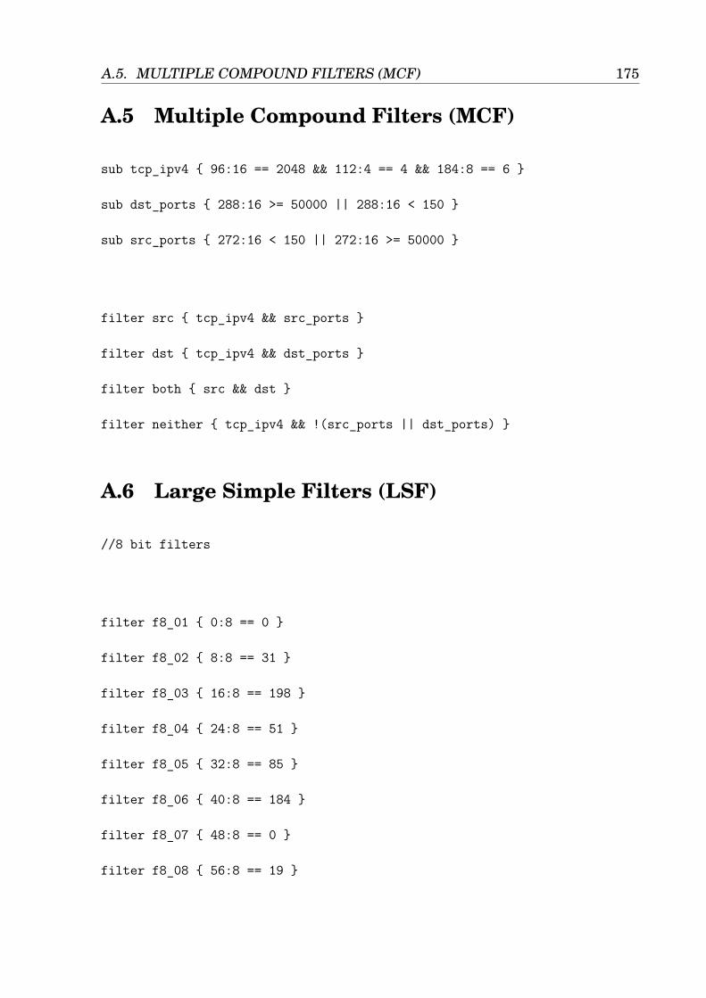
A.5. MULTIPLE COMPOUND FILTERS (MCF) 175
A.5 Multiple Compound Filters (MCF)
sub tcp_ipv4 { 96:16 == 2048 && 112:4 == 4 && 184:8 == 6 }
sub dst_ports { 288:16 >= 50000 || 288:16 < 150 }
sub src_ports { 272:16 < 150 || 272:16 >= 50000 }
filter src { tcp_ipv4 && src_ports }
filter dst { tcp_ipv4 && dst_ports }
filter both { src && dst }
filter neither { tcp_ipv4 && !(src_ports || dst_ports) }
A.6 Large Simple Filters (LSF)
//8 bit filters
filter f8_01 { 0:8 == 0 }
filter f8_02 { 8:8 == 31 }
filter f8_03 { 16:8 == 198 }
filter f8_04 { 24:8 == 51 }
filter f8_05 { 32:8 == 85 }
filter f8_06 { 40:8 == 184 }
filter f8_07 { 48:8 == 0 }
filter f8_08 { 56:8 == 19 }

A.6. LARGE SIMPLE FILTERS (LSF) 176
filter f8_09 { 64:8 == 169 }
filter f8_10 { 72:8 == 130 }
filter f8_11 { 80:8 == 135 }
filter f8_12 { 88:8 == 181 }
filter f8_13 { 96:8 == 8 }
filter f8_14 { 104:8 == 0 }
filter f8_15 { 112:8 == 69 }
filter f8_16 { 120:8 == 0 }
filter f8_17 { 128:8 == 0 }
filter f8_18 { 136:8 == 157 }
filter f8_19 { 144:8 == 21 }
filter f8_20 { 152:8 == 222 }
filter f8_21 { 160:8 == 64 }
filter f8_22 { 168:8 == 0 }
filter f8_23 { 176:8 == 128 }
filter f8_24 { 184:8 == 6 }
filter f8_25 { 192:8 == 78 }
filter f8_26 { 200:8 == 99 }
filter f8_27 { 208:8 == 192 }
filter f8_28 { 216:8 == 168 }
filter f8_29 { 224:8 == 10 }
filter f8_30 { 232:8 == 64 }

A.6. LARGE SIMPLE FILTERS (LSF) 177
//16 bit filters
filter f16_01 { 0:16 == 31 }
filter f16_02 { 8:16 == 8134 }
filter f16_03 { 16:16 == 50739 }
filter f16_04 { 24:16 == 13141 }
filter f16_05 { 32:16 == 21944 }
filter f16_06 { 40:16 == 47104 }
filter f16_07 { 48:16 == 19 }
filter f16_08 { 56:16 == 5033 }
filter f16_09 { 64:16 == 43394 }
filter f16_10 { 72:16 == 33415 }
filter f16_11 { 80:16 == 34741 }
filter f16_12 { 88:16 == 46344 }
filter f16_13 { 96:16 == 2048 }
filter f16_14 { 104:16 == 69 }
filter f16_15 { 112:16 == 17664 }
filter f16_16 { 120:16 == 0 }
filter f16_17 { 128:16 == 157 }
filter f16_18 { 136:16 == 40213 }
filter f16_19 { 144:16 == 5598 }
filter f16_20 { 152:16 == 56896 }

A.6. LARGE SIMPLE FILTERS (LSF) 178
filter f16_21 { 160:16 == 16384 }
filter f16_22 { 168:16 == 128 }
filter f16_23 { 176:16 == 32774 }
filter f16_24 { 184:16 == 1614 }
filter f16_25 { 192:16 == 20067 }
filter f16_26 { 200:16 == 25536 }
filter f16_27 { 208:16 == 49320 }
filter f16_28 { 216:16 == 43018 }
filter f16_29 { 224:16 == 2660 }
filter f16_30 { 232:16 == 25792 }

BList of Publications
This appendix lists the publications that have resulted from this research.
Nottingham, A. & Irwin, B. “Investigating the effect of genetic algorithms onfilter optimisation within packet classifiers.” In Proceedings of the ISSA 2009 Con-ference, Information Security South Africa (ISSA), 2009, pages: 99-116.
Nottingham, A. & Irwin, B. “gPF: A GPU Accelerated Packet Classification Tool.”In Proceedings of the 2009 South African Telecommunication Networks and Ap-plications Conference (SATNAC), Online, 2009. URL http://www.satnac.org.za/proceedings/2009/papers/software/Paper%2063.pdf
Nottingham, A. & Irwin, B. “GPU packet classification using OpenCL: a con-sideration of viable classification methods.” In Proceedings of the 2009 AnnualResearch Conference of the South African Institute of Computer Scientists andInformation Technologists (SAICSIT), 2009, pages: 160-169.
Nottingham, A. & Irwin, B. “Conceptual Design of a CUDA Based Packet Clas-sifier.” In Proceedings of the 2010 South African Telecommunication Networks and
179

180
Applications Conference (SATNAC), Online, 2010. URL http://www.satnac.org.za/proceedings/2010/papers/software/Nottingham%20FP%20v2%20449.pdf
Nottingham, A. & Irwin, B. “Parallel packet classification using GPU co-processors.”In Proceedings of the 2010 Annual Research Conference of the South African Insti-tute of Computer Scientists and Information Technologists (SAICSIT), 2010, pages:231-241.

CContents of Multimedia DVD
The accompanying DVD contains the following directories.
PacketData The packet sets used during testing.
PerformanceData Spreadsheets of performance data, with accompanying graphs.
OutputData Raw classification output, with timings, in compressed text files.
Validation Detailed timing results for validation tests (.csv)
Throughput Detailed timing results for throughput tests (.csv)
Filters Compressed results for SSF, MSF, SCF and MCF filters (.rar)
181