AbstractImage Pyramids, as created during a reduction process of 2D image maps, are frequently used in porting non-local algorithms to graphics hardware. A Histogram pyramid (short: HistoPyramid), a special version of image pyramid, collects the number of active entries in a 2D image. We show how a HistoPyramid can be utilized as an implicit indexing data structure, allowing us to convert a sparse 3D volume into a point cloud entirely on the graphics hardware. In the generalized form, the algorithm reduces a highly sparse matrix with N elements to a list of its M active entries in O(N) + M (log N) steps, despite the restricted graphics hardware architecture. Our method can be used to deliver new and unusual visual effects, such as particle explosions of arbitrary geometry models. Beyond this, the algorithm is able to accelerate feature detection, pixel classification and binning, and enable high-speed sparse matrix compression.

1 IntroductionAs graphics hardware has become more pro-grammable, new applications like general matrix calculation, sorting applications or physics pro-cessing have become feasible (e.g. [5], [7], [12],

[2]). But ever since the first of these applications had been implemented, it had been clear that the stream processing nature of graphics hardware, which gives it tremendous processing power, also requires considerable rethinking of data structures and algorithms. Many non-local calculations, which are virtually trivial on single-thread sys-tems, become hard to solve on the GPU. Its inher-ently parallel nature can only be utilized if the out-put of several independent parallel units is com-bined. It is not allowed to forward data from one output element to the next one. The thought model of data pyramids showed how a global sum of values can be computed: A so-called reduction operator ([1]) repeatedly sums groups of four cells in a pyramidal data array, until only one cell prevails. We call the data array a his-togram pyramid, or HistoPyramid. Now, in our task, after the 3D model has been ras-terized into a 3D volume, a list of occupancies must be generated. The 3D volume resides in GPU memory after rasterization. Due to above reasons, we cannot apply the trivial CPU solution to occu-pancy testing, which would traverse the data se-quentially in order to count all occupied pixels, and grow a list of cell coordinates. Instead, we have devised a completely GPU-based algorithm which uses the mentioned HistoPyra-

On-the-fly Point Cloudsthrough Histogram Pyramids

arbrücken, GermanyGernot Ziegler, Art Tevs, Christian Theobalt, Hans-Peter Seidel

Max Planck Institute for Informatics, Computer GraphicsStuhlsatzenhausweg 85, D-66121 Saarbruecken, Germany

Email: {gziegler, tevs, theobalt, hpseidel}@mpi-inf.mpg.de

Figure 1: Dicer, our demo application, decomposing a teapot into a point cloud on the GPU, by rendering it repeatedly into slices of a 256x256x256 volume (marked in red). The volume is filled with approximately 34000 surface points. Left to right: 3D model of teapot; volume slices at z=70/130/190/201; resulting particle cloud calculated after 91 ms.

mid. For each point list entry to be generated, it traverses the histogram pyramid from the top level downwards until the corresponding point has been found. The histogram pyramid thus serves as an implicit indexing data structure.We test the algorithm's practical use in Dicer, an application which converts arbitrary 3D models into particle clouds in real-time, running complete-ly on the GPU.

2 Related WorkImage pyramids have been used in Binary Tree Predictive Coding, e.g. [4] and [11]. For example, a quad tree leaf can signal if all of its descendants are identical, and hence skip the transmission of its descendants. Our algorithm uses similar ideas to skip empty regions during the top-down HistoPy-ramid traversal, which builds up the point list.The build process for the mentioned HistoPyramid is adopting the well-known parallel "reduction op-eration". It is applied in custom mipmapping (see also [1]), and processes n2 elements in log2(n) passes. Our sum operator builds a hierarchy of partial histograms. One variant of our algorithm uses bilinear texture interpolation to accelerate the summing operation, similar to [8], see section 7.2. Other GPU-based spatial data structures include indirection tables, N3 trees and octrees, see [2]. [9] maps perfect spatial hashing onto graphics hard-ware. Those data structures are more memory-effi-cient than our solution, but none of them can be generated directly by the graphics hardware. Bitonic merge sort, as exemplified in [3], could also be used for point isolation in sparse images by giving seed points a different sorting key than in-

valid points. However, since this sorting algorithm is optimized for a plentiful of key values, it runs suboptimally ( O(n (log n)2) steps) for a 2D image where only a binary partitioning is required.Finally, [6] introduces the concept of data com-paction, i.e. filtering of unwanted data elements from a given data stream. It does this by succes-sively producing a running sum, describing where to skip unwanted elements to obtain a packed re-sult. The algorithm needs log(n) iterations to pro-duce this running sum, and keeps the number of output elements constant. [13] improves on [6] by utilizing all intermediate data levels in the point list reconstruction, a reduc-tion from log2(n)·n to 2·n data elements in the in-termediate data output. Our algorithm uses a similar reduction as [13], but in 2D space (cell coverage: 2x2), in contrast to the 1D nature (1x2) of [6] and [12]. This maps closer to the GPU's 2D image storage and texture caching mechanisms. As a consequence, we can utilize the GPU's bilinear texture interpolation if it yields an advantage. Our approach omits the assumption of a certain number of processors to keep the algo-rithm general for future GPU generations. We fur-ther propose a vec4-vectorization variant that ac-celerates traversal, at the expense of extra memory, see Section 7.

3 Overview Figure 2 illustrates the workflow between the dif-ferent computation steps. The figure omits the triv-ial 3D volume to 2D image conversion, and exem-plifies the point cloud generation with the help of a 2D image. All data is being processed on the

Figure 2: Overview over the internal workflow. (Omits voxelization).

HistoPyramidBuilder

PointListBuilderDiscriminator

HistoPyramid

PointListActive/inactiveInput image

0 1 10 1 02 0 20 2 2 0

10

024 4

212

(5,1)(2,1)(0,4)(2,2)

(1,5)(5,2)(7,4)(2,6)

(4,6)(3,6)

(5,6)(6,5)

GPU – the CPU is only handling data if the point list shall be downloaded for further processing in a non-GPU application. After 3D model rasterization, the input data has become a 2D image, filled with volume slices. The image cells may be of arbitrary type (single/RGBA, byte/float), as long as the Discrimi-nator is able to handle cells of such type. The Discriminator decides if a cell's content is re-garded as active (1) or not (0). Section 4 explains the details. The HistoPyramid Builder creates the data pyra-mid of partial histograms from the discriminator output. Its reduction operator repeatedly processes four input cells into one, starting at the resolution level of the original input image. It finishes when only one output cell remains. We describe its GPU implementation in Section 5. The PointList Builder takes the HistoPyramid, creates a 2D array of coordinates, called a point list, and fills every list entry by using a hierarchi-cal traversal of the HistoPyramid. Section 6 de-scribes details of the traversal in diagrams, and presents a log of the traversal decisions. Moreover, we shortly mention how the 3D point cloud can be trivially reconstructed from this 2D point list. Fur-ther, it is discussed which GPU restrictions ham-per performance, and how their removal might im-prove future implementations. We have also devised algorithmic variants, in-cluding one which uses the GPU's native vector capabilities, and a version which utilizes bilinear texture interpolation. A discussion of these vari-ants can be found in section 7.The basic, or, for CPU programmers, fairly straightforward concepts underlying our algorithm can make it hard to understand the full range of new applications that a GPU implementation opens. Therefore, section 8 outlines several real-time applications that become feasible with a GPU implementation of this algorithm.Section 9 summarizes the current performance re-sults that we obtained by running the algorithm's variants on state-of-the-art graphics hardware. It describes the surrounding test setup, and analyzes their runtime behaviours.

4 DiscriminatorThe subsequent stages operate on binary data, each cell has to be either active (1) or not (0). Therefore, we must first preprocess our input data.

Our Dicer demo earmarks voxels which are active, i.e. which are occupied by the 3D model, with alpha=1.0. As alpha thresholding is a local and inexpensive operation, it was integrated into the first stage of the HistoPyramid Builder. This saves storage space and calculation time, since the dis-crimination results never have to be written to video memory. It should be noted, though, that PointList Builder has to redo these operations on the base level to determine if it has found the cor-rect target cell. Therefore, it is only advisable to use this variant if the discrimination operator's cal-culation costs are negligible in comparison to writ-ing and re-reading the binary image. Beyond this simple discriminator, any operator which maps 2D image cells into such a binary de-cision can be utilized here. We refer to [14] for a more extensive survey of applicable discrimination operators.

5 HistoPyramid BuilderThe HistoPyramid, short for histogram pyramid, is a pyramid of partial histograms with the Discrimi-nator's binary output as its base. On this base level, each active cell is treated as a 1, while inactive or empty cells are interpreted as 0. Our reduction op-erator simply sums up four underlying cells and writes the result into the prepared output level im-age until the final level consists of only one cell. The algorithm annotates the level of this cell (the top level) for the subsequent stages, and termi-nates. The output is a stack of 2D arrays with inte-

ger content (2D textures with 32bit float values in the GPU implementation), see Figure 3.

Figure 3: Basic HistoPyramid building process. L0, L1 and L2 are the pyramid levels. The GPU repeatedly sums four adjacent cells, every time halving resolution, until only one cell remains.

2231

8

L0(Base, 4x4)

L1(2x2)

L2(Top, 1x1)

Red

uce

Sum cell content(reduction operation)

Red

uce

1

1

11

1

100

00

00 11

0

0

6 PointList BuilderGiven the HistoPyramid as input, it is now possi-ble to determine the number of list entries. PointList Builder accesses the top level of the pyramid to retrieve this value, and allocates the point list, a 2D array with a sidelength equal to the square root of the number of entries (see Figure 4 for an example 2D point list). The reason for choosing a 2D layout is that the GPU currently only can handle 4096 entries at maximum in a 1D image. The GPU treats this array as 2D image.Now, actual point list reconstruction commences. In our example in Figure 4, the PointList Builder shader will now be called for all nine possible list entries in the 2D image.The shader first determines its own index (the key index) from its 2D coordinate in the point list. Since it has also been given the total number of entries (the list count, here: 8), it immediately ter-minates if the key index exceeds the list count (such an entry is only an artifact from the 2D im-age allocation - our example marks it with an X). The algorithm descends if the key index lies within the index range of a HistoPyramid cell. Intuitively, the index range of a HistoPyramid cell describes the covered range of key indices that active cells in this covered part of the 2D input image can re-ceive. The top level's single cell poses a good ex-ample, its range covers all active cells' indices.

A different way to see it is that all active cells in a given index range will be quadtree children of this cell. During traversal of the HistoPyramid, the current index range [start, end] is updated as follows: • start is initialized to zero. • end is assigned the sum of the cell's content

(looked up from the HistoPyramid) and start. • Before a new cell is examined on the same level,

start becomes the former index range end.• A descend happens if the key index falls into

[start;end[ . On descend, we retain the start val-ue of the pre-descend range check.Note that the traversal order is irrelevant as no

sorting is enforced; it only needs to be the same order for all point list entries to avoid doublettes. That is certainly fulfilled as the PointList Builder shader is the same for all pixels. The descend repeats until the base level has been reached. There, the final target cell is chosen after the same index range criterion, if we interpret an active cell as a value of 1. The target cell's coordi-nates are written into the point list output.The final result is thus a 2D array containing coor-dinate entries of all active cells in the image, the point list. PointList Builder assigns a unique active cell to each index, but the indexing order is some-what unintuitive (based on a fractal traversal pat-tern). Optionally, the algorithm can provide line-

Figure 4: PointList Builder's internal data traversal for an example key index. Left: graphical illustration. Right, top: naming convention for lookup directions, as seen from a parent cell O. Right bottom: Algorithm's log on made decisions.

11

1

11

1

1

10

0

00

00

02

231

8

L0

L1

(1,0)

(0,3)

(0,0)(2,1)(0,1)

(1,2)(3,2)

(3,0)X

: traversal direction

Output:2D Point List

L2

2

6

041

57

3(8)

Input: Key indices

0

Example traversal, key index 4

HistoPyramid, traversal path:

(2D list size: (plw, pwh) = 3 x 3)

PointList Builder, run at (px, py)=(1,1):• Key index: ki = py * plw + px = 4• L2: Index Range [0,8[ : fits !• (descend to L1, retain start=0)• L1, cell UL: Index Range [0,3[• L1, cell UR: Index Range [3,5[ :fits !• (descend to L0, retain start=3)• L0, cell UL: empty• L0, cell UR: Index Range [3,4[• L0, cell LL: Index Range [4,5[ : fits !• Result: (2,3)

UR: upper rightUL: upper left

LL: lower left LR: lower right

P

wise indexing if a line-wise CPU traversal is de-sired. In that case, the reduction operator takes four horizontal cells instead of a square of 2x2. However, this would probably hamper texture caching performance during the HistoPyramid construction.For the point cloud application, the presented gen-eral algorithm is modified: When the final 2D co-ordinates of each active cell have been found, we convert them back into 3D voxel space coordi-nates and output them instead.The GPU thus needs 4log2 max sizex ,size ytexture accesses to generate one point in the list.

7 Algorithmic variantsWe have developed a couple of algorithmic vari-ants to the core method in order to speed up the pipeline. Two of them are explained here, please refer to [14] for more details on point list stretch-ing. and the pros and cons of merging Discrimina-tor with HistoPyramid Builder.

7.1 Faster traversal with partial sums in vec4

This variant makes use of the GPU's vector capa-bilities. As it is capable of manipulating four float values in each target cell, we store the partial sums of the leaf cells in the parent cell, instead of only the overall sum (see Figure 5). We call this the vec4-HistoPyramid.In this pyramid, it is not necessary to do four tex-ture lookups (in the leaf cells) to decide in which quadtree branch to descend. Instead, this decision can already be made based on the partial sums in the level above. The algorithm needs only needs

log2maxsizex ,size y texture accesses, and

can thus save up to three of them for every tra-versed HistoPyramid level.

7.2 Bilinear interpolation for faster sum-up

This variant uses the GPU's bilinear texture inter-polation. Our interpolation-based HistoPyramid Builder places a texture lookup exactly in the mid-dle between the four input cells of the level below, which makes texture interpolation return the aver-age of the four input cell values. A multiply with four yields the sum. This is faster than calculating the sum in the shader, since graphics hardware contains special data paths for such interpolated lookups. Unfortunately, current hardware restricts such interpolation to 16 bit float values. As 16 bit floats are not enough to represent more than 32768 points, we have devised a way to split a 20 bit in-teger into two 16 bit floats. But such a splitting re-quires constant rebalancing of the interpolated val-ues in the HistoPyramid Builder, and an extra dot product to reconstruct cell values in PointList Builder. Also note that interpolation cannot easily be combined with the vec4-HistoPyramid from section 7.1.

8 ApplicationsBesides the mentioned point cloud generation, we see several other potential applications for HistoPyramid Builder and PointList Builder.

8.1 Image analysis

The most promising application for this algorithm is solving computer vision problems solely on graphics hardware. As an example, GPUs can now analyze the image convolution result after con-ducting the actual folding, and thus augment the algorithms proposed in [12], see [14] for the re-quired, more advanced discrimination operators. The expensive download of half-processed image data can thus be avoided, and only the discovered feature point set needs to be transferred.

8.2 Volume analysis

We have currently only described how to analyze volumes after conversion into a 2D image, but the algorithm can directly handle 3D volumes if the HistoPyramid became a hierarchy of 3D volumes. Unfortunately, current render-to-texture function-ality can only write to one 2D slice at a time (if at all: NVidia drivers currently do not support that), which slows down performance due to framebuffer setup times.

Figure 5: dicer_vec4's extended RGBA storage and the modified reduction operator.

L0(Base, 4x4)

L1(2x2)

L2(Top, 1x1)

Red

uce

Other levels:Sum up vec4's

Red

uce

11

1

11

1

1

10

0

0000 0

0 232 1

Base: create vec4's

GRB A

G=dot(UR,1)R=dot(UL,1)B=dot(LL, 1) A=dot(LR,1)

1

1

11

1

100

00

00 11

0

0

Layout, vec4 Reduction operator, vec4

L0(Base, 4x4)

L1(2x2)

L2(Top, 1x1)

11

1

11

1

1

10

0

0000 0

0 232 1

GRB A

G=dot(UR,1)R=dot(UL,1)B=dot(LL, 1) A=dot(LR,1)

1

1

11

1

100

00

00 11

0

0

Layout, vec4 Reduction operator, vec4

As a proof of concept, we have recently used this algorithm for detecting seed points in 3D flow data on the GPU. We are very confident that other ap-plications, such as level-set identification, are pos-sible. Even a GPU based marching cubes algo-rithm is within reach, provided that the algorithm can generate geometry after the relevant voxel/mesh mappings have been identified.

8.3 Sparse matrix creation

[7] has demonstrated how to process large sparse matrices by packing them into a special represen-tation. Until now, it has not been possible to cre-ate such sparse matrix representation on graphics hardware. Our algorithm could be used to convert matrices into such sparse matrix representations, and thus save memory and computation time.

8.4 Quadtree Builder

Many simulation problems deal with processing data of varying sample density (e.g. fluid simula-tions, [5] or [7]). Also, compression and encoding often require the clustering of similar regions. HistoPyramid Builder can be modified to count the largest-size regions of common cell values, and to mark at which level they are found in the hierar-chy. PointList Builder can in that case output a quadtree whose leafs terminate at the level where only identical values remain. This way, computa-tion and storage could adapt to sample density, in much the same spirit as sparse matrix computa-tions do not waste resources on empty regions.

9 ResultsIn order to test the real-time behaviour of our algo-rithm, we implemented Dicer, a small Linux appli-cation that converts 3D models to point clouds. The 3D model, a teapot generated with glut-Teapot(0.6), is stored in a display list to maxi-mize geometry throughput. The software voxelizes the mesh by rendering it into 256 2D slices of 256x256 each, spanning a volume of [-1,-1,-1] to [1,1,1] in world space (see also Figure 1). The out-put is put into 16 x 16 tiles of an 8-bit RGBA tex-ture at 4096x4096 resolution. All pixels belonging to the 3D model are marked with alpha=1.0. Additionally, we experiment with smaller texture sizes to measure the performance scaling, effec-tively producing volumes of 256x128x128 (2048x2048) and 256x64x64 (1024x1024). After voxelization, the algorithm analyzes the re-sulting 2D texture and generates the point cloud

from the marked pixels. Typically, it finds around 33000 points, and renders them as a particle cloud. The tests were conducted on a Dell Precision M70 laptop with Nvidia Quadro FX Go 1400 and 256 MB video memory, connected over PCI Express. It contained an Intel Pentium M (2.13 Ghz) and 2 GB of main memory. The AGP download timings came from an Athlon XP2400 system with an Nvidia GForce 6600, AGP 8x. We compare four variants of the algorithm:dicer_single is the most classic implementation, and follows the basic algorithm in Figure 4. It uses the OpenGL texture format GL_TEXTURE_2D, which provides mipmaps and render-to-texture, but current restrictions force it to build the HistoPyramid in a 32 bit-float RGBA texture, even though only one data channel is used. dicer_vec4 is similar, but makes better use of the four 32-bit components by storing partial sums in the RGBA vec4, effectively delaying the cell sum-up by one level (see Figure 5 and section 7.1). This accelerates PointList Builder, as the tree traversal has do to less texture lookups to make its branching decisions.dicer_rect utilizes GL_TEXTURE_RECTANGLE, a texture format without mipmaps - but render-to-texture allows 32-bit single float textures here, which saves considerable amounts of memory. Since PointList Builder needs to access all levels in one pass, we were forced to create a pseudo-mipmap layout in a single texture (see Figure 6).

dicer_bil is similar to dicer_single, but uses bilin-ear texture interpolation to accelerate the HistoPy-ramid construction, as proposed in section 7.2. Unfortunately, the algorithm proved to be numeri-cally unstable. It could not faithfully reproduce a complete list of active cells in a test image, and was thus skipped in evaluation. We will verify this algorithmic variant with the forthcoming bilinear texture interpolation for 32-bit float values in Shader Model 4.0.

Figure 6: dicer_rect's pseudo-mipmap layout for rectangular textures without mipmap capability.

2231

8

L0 L1 L2

XX

XX

XX

XX

XX

X

(unused)

1

1

11

1

100

00

00 11

0

0

We could not test the algorithm on ATI graphics hardware without intense redesign due to the ATI driver's OpenGL API restrictions. Table 1 lists the timings common to all implemen-tations. Slicing (the voxelization of the 3D model into a 2D texture) dominates all timings, presum-ably due to the repeated geometry processing. Instead of taking the time consumed by the OpenGL call delays on the CPU side, we measured actual GPU timings with the GL_EXT_timer_query extension ([10]). For Table 2, we implemented a classic CPU loop to compare our GPU algorithm with a standard single-thread implementation. Here, the CPU downloads the 2D volume texture as RGBA8 (over AGP or PCI express, depending on the sys-tem), generates an output list after line-wise traver-sal, and uploads it to the GPU again. Aggressive compiler optimization accelerates the CPU based analysis. No SIMD techniques were used. CPU timings were taken as virtual process time by the getitimer() function of Linux systems. It is clear that for large textures, the texture download greatly outweighs the actual analysis.Table 3 shows the GPU time spent for creating the HistoPyramid. Both dicer_single and dicer_vec4 suffer heavily from the restriction to RGBA, 32-bit float textures: The texture data is obviously being swapped to main memory, causing large perfor-mance penalties for 4096x4096. dicer_rect can use single-component 32-bit float textures, and there-fore scales as expected. Even without memory re-strictions, render-to-texture is considerably faster for single components than for RGBA.

Table 1: Timings common for CPU and GPU variants.

4096x4096 2048x2048 1024x1024Voxelize 470 ms 470 ms 470 msVoxel count

33989 8595 2130

Table 2: CPU: Timings for whole traversal.

4096x4096 2048x2048 1024x1024AGP fetch 560 ms 142 ms 36 msPCIe fetch 172 ms 40 ms 12 msCPU traversal 25 ms 25 ms 24 ms

Table 3: GPU: HistoPyramid creation for variants.

4096x4096 2048x2048 1024x1024dicer_single ~2000 ms 20 ms 6 msdicer_vec4 ~2000 ms 20 ms 6 msdicer_rect 30 ms 10 ms 2 ms

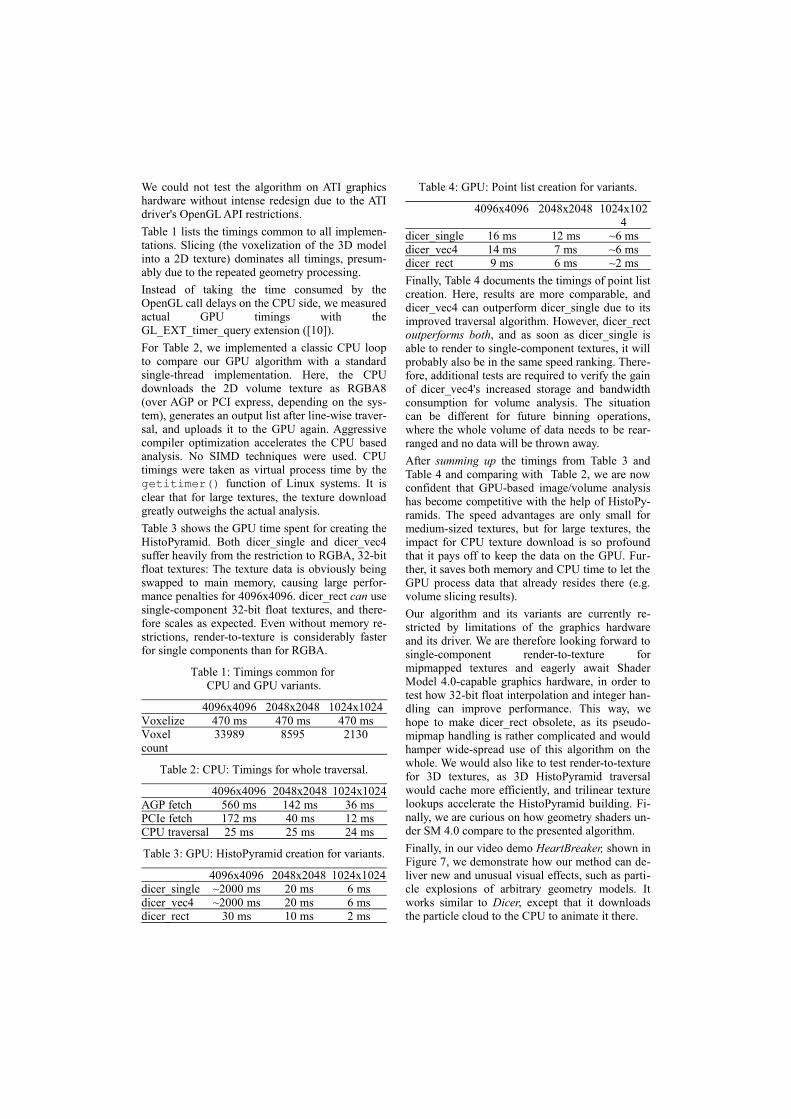
Table 4: GPU: Point list creation for variants.

4096x4096 2048x2048 1024x1024

dicer_single 16 ms 12 ms ~6 msdicer_vec4 14 ms 7 ms ~6 msdicer_rect 9 ms 6 ms ~2 msFinally, Table 4 documents the timings of point list creation. Here, results are more comparable, and dicer_vec4 can outperform dicer_single due to its improved traversal algorithm. However, dicer_rect outperforms both, and as soon as dicer_single is able to render to single-component textures, it will probably also be in the same speed ranking. There-fore, additional tests are required to verify the gain of dicer_vec4's increased storage and bandwidth consumption for volume analysis. The situation can be different for future binning operations, where the whole volume of data needs to be rear-ranged and no data will be thrown away. After summing up the timings from Table 3 and Table 4 and comparing with Table 2, we are now confident that GPU-based image/volume analysis has become competitive with the help of HistoPy-ramids. The speed advantages are only small for medium-sized textures, but for large textures, the impact for CPU texture download is so profound that it pays off to keep the data on the GPU. Fur-ther, it saves both memory and CPU time to let the GPU process data that already resides there (e.g. volume slicing results).Our algorithm and its variants are currently re-stricted by limitations of the graphics hardware and its driver. We are therefore looking forward to single-component render-to-texture for mipmapped textures and eagerly await Shader Model 4.0-capable graphics hardware, in order to test how 32-bit float interpolation and integer han-dling can improve performance. This way, we hope to make dicer_rect obsolete, as its pseudo-mipmap handling is rather complicated and would hamper wide-spread use of this algorithm on the whole. We would also like to test render-to-texture for 3D textures, as 3D HistoPyramid traversal would cache more efficiently, and trilinear texture lookups accelerate the HistoPyramid building. Fi-nally, we are curious on how geometry shaders un-der SM 4.0 compare to the presented algorithm.Finally, in our video demo HeartBreaker, shown in Figure 7, we demonstrate how our method can de-liver new and unusual visual effects, such as parti-cle explosions of arbitrary geometry models. It works similar to Dicer, except that it downloads the particle cloud to the CPU to animate it there.

10 Conclusions and OutlookWe have presented a novel, fast and easy-to-use GPU algorithm for rapidly generating point clouds from 3D volume data or 3D models. Some new, impressive visual effects for the development of computer games are now feasible. Other possible applications for this technology are numerous, ranging from GPU-based computer vi-sion applications, such as 2D image analysis or feature detection, over 3D volume processing, such as occupancy testing or seed point selection to improved efficiency in general GPU calcula-tions.Through experiments we have shown that our purely GPU-based implementation is significantly faster than a hybrid GPU/CPU implementation.Despite the current limitations, we have presented a versatile algorithm with a multitude of applica-tions. It will be highly interesting to see how it maps into image analysis, data compression and general purpose computation. Recent investigation also found that this algorithm could contribute im-proved performance of the Glift library ([2]). In general, there should now only be few computa-tional tasks left that can not be done on GPUs.

References[1] I. Buck and T. Purcell. A Toolkit for

Computation on GPUs. GPU Gems, pp.621-636,2004.

[2] A. Lefohn, J. Kniss, R. Strzodka, S. Sengupta and J. Owens. Glift: Generic, efficient, random-access GPU data structures. ACM Transactions on Graphics 25, 2006.

[3] N. Govindaraju, M. Henson, M. Lin and D. Manocha. Computations among Geometric Primitives in Complex Environments. Proc. ACM Symposium on Interactive 3D Graphics and Games, 2005.

[4] S. Hanan. Data structures for quadtree approximation and compression. Communications of the ACM, Volume 28, Issue 9, pp. 973-993, 1985.

[5] M. Harris. Fast Fluid Dynamics Simulation on the GPU. GPU Gems, pp.637-665,2004.

[6] D. Horn. Stream Reduction Operations for GPGPU applications. GPU Gems 2, pp. 621-636, Addison-Wesley.

[7] J. Krüger and R. Westermann. Linear algebra operators for GPU implementation of numerical algorithms. Proc. ACM SIGGRAPH 2003, pp. 908-916, 2003.

[8] S. Green, NVidia Corp. OpenGL Image Processing Tricks. GDC 2005 Presentations, 2005. http://tinyurl.com/f59r4

[9] S. Lefebvre, H. Hoppe. Perfect Spatial Hashing. ACM SIGGRAPH 2006, to appear.

[10] S. Green, NVidia Corp. NVidia OpenGL Update. GDC 2005 Presentations, 2005, pp. 40-42. http://tinyurl.com/pngld

[11] J A Robinson. Efficient General-Purpose Image Compression with Binary Tree Predictive Coding. IEEE Transactions on Image Processing, Vol 6, No 4, April 1997, pp 601-607.

[12] J. Fung and S. Mann. OpenVIDIA: parallel GPU computer vision. Proc. 13th annual ACM international conference on Multimedia, 2005, pp. 849 - 852. http://openvidia.sf.net

[13] S. Sengupta, A. E. Lefohn, J.D. Owens: A Work-Efficient Step-Efficient Prefix Sum Algorithm. Proc. 2006 Workshop on Edge Computing Using New Commodity Architectures, pp. D26-27.

[14] G. Ziegler, A. Tevs, C. Theobalt and H-P. Seidel. GPU Point List Generation through Histogram Pyramids. Technical Reports of the MPI for Informatics, June 2006, MPI-I-2006-4-002.

Figure 7: Screenshots of our FX demo HeartBreaker. From left to right: Solid model (5000 triangles); Point cloud representation (1872 points, in a 256x64x64 grid, first iteration: 90 ms, subsequently: 25 ms); Particle explosion effect.

Figure 7: Screenshots of our FX demo HeartBreaker. From left to right: Solid model (5000 triangles); Point cloud representation (1872 points, in a 256x64x64 grid, first iteration: 90 ms, subsequently: 25 ms); Particle explosion effect.

Figure 1: Dicer, our demo application, decomposing a teapot into a point cloud on the GPU, by rendering it repeatedly into slices of a 256x256x256 volume (marked in red). The volume is filled with approximately 34000 surface points. Left to right: 3D model of teapot; volume slices at z=70/130/190/201; resulting particle cloud calculated after 91 ms.

Figure 7a: Wireframe model of the Heart mesh before point cloud conversion. Figure 1a: Layout of the generated point list. XYZ

coordinates have been encoded into RGB values.