granger causality for ill-posed...

Granger Causality for Ill-Posed ProblemsMethods, Ideas and Application in Life Sciences

Katerina Hlavackova-Schindler

Department of Adaptive SystemsInstitute of Information Theory and AutomationAcademy of Sciences of the Czech Republic

Prague, Czech Republic

Statistics and Causality, University of ViennaAustria, May 23-24, 2014

K. Hlavackova-Schindler Granger Causality for Ill-Posed Problems Statistics and Causality 2014 1 / 42

Outline

1 Introduction

2 Causality problems in neurology (brain research)and biology (gene regulatory networks)

3 Brief introduction to inverse problems

4 Granger causality and multivariate Granger causality

5 Our two-level thresholding method

6 Application to a gene regulatory network and comparison toother methods

7 Conclusion and outlook


Introduction

Concept of causality by Granger 1969

1 an econometric concept

2 a probabilistic concept, relating to the ability of one time series topredict another one, conditional on a given information set;

Concept of causality by Pearl 2000

1 a direct causality concept

2 addresses interventions rather of functional than of probabilisticdependence

White, Chalak, Lu, 2011:Granger and Pearl’s concepts are in fact closely linked: straighforwardpractical methods to test direct causality in Pearl’s sense using Grangercausality were proposed.Bivariate Granger causality; multivariate Granger causality:


Problems in Brain Research

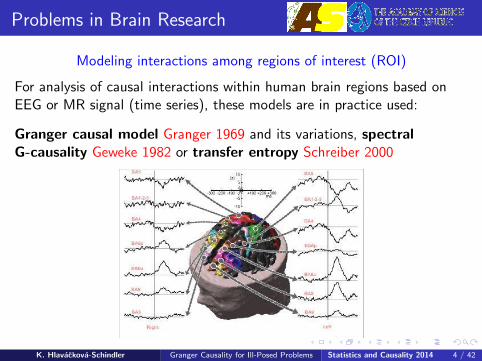
Modeling interactions among regions of interest (ROI)

For analysis of causal interactions within human brain regions based onEEG or MR signal (time series), these models are in practice used:

Granger causal model Granger 1969 and its variations, spectralG-causality Geweke 1982 or transfer entropy Schreiber 2000


Problems in Genetics

A gene regulatory network or genetic regulatory network (GRN)

is a collection of DNA segments in a cell which interact with eachother indirectly (through their RNA and protein expression products)and with other substances in the cell, thereby governing theexpression levels of mRNA and proteins.

Biological cells can be thought of as ”partially mixed bags” ofbiological chemicals: these chemicals are mostly the mRNAs andproteins that arise from gene expression. These mRNA and proteinsinteract with each other with various degrees of specificity- gene regulatory networks. (Source: Wikipedia)

Gene expression is the process by which the information encoded ina gene is used to direct the assembly of a protein molecule. Theseproducts are often proteins.


Problems in Genetics

Structure of a gene regulatory network (source: Wikipedia)


Application in genetics

A gene regulatory network - a formal simplification1 directed graph:

nodes - genesedges - interactions between genes

2 Data:each node is given by a time series of gene expressions(expressions of proteins)

3 Unknown - the directed edges


Gene regulatory networks

Methods for recovery of gene regulatory networks:

Dynamic Bayesian networks, structural equation models,probabilistic Boolean networks, petri nets, graphical Gaussianmodels, fuzzy controls and differential equations. - A goodmodeling of small regulatory networks for which biologicalinformation is available (local kinetics).

For large networks: Due to small data sets (observations) and highdimensionality of the microarrays (a collection of microscopic DNAspots attached to a solid surface) these models suffer fromcurse of dimensionality (exp. search space) and the relatedparameter estimation problems are ill-posed.

An alternative which overcomes these deficits:Graphical Granger models


Inverse Problems

A short introduction to Inverse Problems

Definition by Engl, Hanke, Neubauer 1996:Inverse problems are concerned with determining causes for a desiredor an observed effect.The inverse problem (IP) is considered the ”inverse” to the direct problemwhich relates the model parameters to the data that we observe:

direct problem⇒

CAUSE EFFECTparameters, data,

unknown solution of IP observations

⇐inverse problem


Direct and Inverse Problems

The classification as direct or inverse is in the most cases based on thewell/ill-posedness of the associated problems:

stable⇒

Cause Effect⇐

unstable

Inverse problems v Ill-posed/(Ill-conditioned) problems


Well posed and Ill posed problems

A central feature of inverse problems is their ill-posedness

Well-Posedness in the sense of Hadamard 1923

Existence of a solution (for all admissible data)Uniqueness of a solutionContinuous dependence of solution on the data

Well-Posedness in the sense of Nashed 1987A problem is well posed if the set of data/observations isa closed set. (The range of the forward operator is closed).


Abstract Inverse Problem

Abstract inverse problem:

Solve equation for x ∈ X (Banach, Hilbert space), given datay ∈ Y (Banach, Hilbert space)

F (x) = y

where F−1 does not exist or is not continuous.

F is the forward operator and we want to findx† the (generalized) solution so that

x† = F−1(y).

If the forward operator is linear then it is a linear inverse problem.


Well-posed and Ill-posed problems

Problems that are not well-posed in the Hadamard sense areill-posed.

Inverse problems are often ill-posed(the solution is highly sensitive to changes in data).

Continuum models must often be discretized in order to obtain anumerical solution. While solutions may be continuous w. r. t. theinitial conditions, they may suffer from numerical instability whensolved with finite precision, or with errors in the data.

Even if a problem is well-posed, it may still be ill-conditioned(i.e. a small error in the initial data can result in much larger errorsin the answers.)

An ill-conditioned problem is indicated by a large condition number.


Methods to solveIll-posed problems

If the problem is well-posed then it stands a good chance of solutionon a computer using a stable algorithm.

If it is not well-posed, it needs to be reformulated for numericaltreatment. Typically this involves including additional assumptions,such as smoothness of solution.

This process is known as regularization.

The most applied regularization methods areTikhonov regularization (ridge regression), elastic nets,Lasso or bridge regression (lq norms).


Regularization

Penalty as a stabilizator of the least means square problem (LMS):If parameters (the solution) of LMS are unconstrained, they have veryhigh variance. To control variance, we might regularize the coefficientsby imposing the penalty

l2 penalty - Tikhonov regularization(ridge regression in statistics)

‖y − Xβ‖2 + λ‖β‖22 → minβ. (1)

where ‖β‖22 =∑

j β2j and λ is a tuning parameter controling

the amount of regularization.

l1 penalty - Lasso penalty(sometimes called l1-Tikhonov regularization)


Lasso Penalty

l1 penalty - Lasso penalty(Least absolute shrinkage and selection operator)introduced by Tibshirani in 1996

LASSO coefficents are the solutions to the l1 optimization problem:

‖y − Xβ‖2 + λ‖β‖1 → minβ. (2)

where ‖β‖1 =∑

j |βj | and λ is a tuning parameter controling theamount of regularization.

Often we believe that many of the β′js should be 0.

Hence we look for a set of sparse solutions.

Large enough λ will set some coefficents exactly equal to 0.

Lasso is therefore a model selection method. Its tendency tooverselect variables will be addressed by our two-level thresholdingalgorithm.


Back to genetics

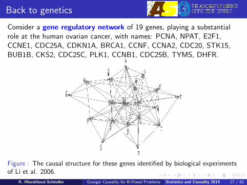
Consider a gene regulatory network of 19 genes, playing a substantialrole at the human ovarian cancer, with names: PCNA, NPAT, E2F1,CCNE1, CDC25A, CDKN1A, BRCA1, CCNF, CCNA2, CDC20, STK15,BUB1B, CKS2, CDC25C, PLK1, CCNB1, CDC25B, TYMS, DHFR.

Figure : The causal structure for these genes identified by biological experimentsof Li et al. 2006.


Graphical Granger models

Gene regulatory network (GRN)

1 For each of 19 genes (graph nodes) given gene expressionsfor 48 time observations (data).Problem: Find the values of edges of the graph on the nodes.

2 The problem is ill-posed - Multivariate Granger causality (MVAR)will not suffice

3 Graphical Granger models = multivariate Granger causality modelwith various regularizations:

Lozano et al. 2009 Grouped Granger method- uses group elastic net (combination of l1 and l2 penalties)Arnold et al 2007 (Lasso)Shojaie 2010, 2012 Truncated Lasso, Adaptive thresholding 2010, 2012

4 Our approach:Two-level thresholding for reconstructing gene regulatory networksPereverzyev, Hlavackova-Schindler, 2013


Granger Causality

Granger Causalitybased on the probabilistic notion of causality, is defined:An event X is a cause to the event Y if(i) X occurs before Y ,(ii) likelihood of X is non zero, and(iii) likelihood of occurring Y given X is more than the likelihoodof Y occurring alone.It is said that the process Xt Granger causes another process Yt

if future values of Yt can be better predicted using the past valuesof Xt and Yt rather then only past values of Yt .


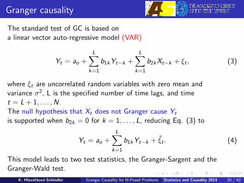
Granger causality

The standard test of GC is based ona linear vector auto-regressive model (VAR)

Yt = ao +L∑

k=1

b1kYt−k +L∑

k=1

b2kXt−k + ξt , (3)

where ξt are uncorrelated random variables with zero mean andvariance σ2, L is the specified number of time lags, and timet = L + 1, . . . ,N.The null hypothesis that Xt does not Granger cause Yt

is supported when b2k = 0 for k = 1, . . . , L, reducing Eq. (3) to

Yt = ao +L∑

k=1

b1kYt−k + ξt . (4)

This model leads to two test statistics, the Granger-Sargent and theGranger-Wald test.


Multivariate Granger causality

Extension of GC to more than two time series:A multivariate vector autoregressive model MVAR: graphical Grangermodels.Based on the intuition that the cause should precede its effect,in Granger causality one says that a variable x i can be potentially causedby the past versions of the involved variables {x j , j = 1, . . . , p}.Then, in the spirit of the statistical approach we consider the followingapproximation problem:

x it ≈p∑

j=1

L∑l=1

βjl xjt−l , t = L + 1, . . . ,T , (5)

where L is the so called maximal lag, which is the maximal number ofthe considered past versions of the variables.


Multivariate Granger causalitythreshold parameter

The approximation problem x it ≈p∑

j=1

L∑l=1

βjl xjt−l , t = L + 1, . . . ,T , can be

specified using the least-squares approach:

T∑t=L+1

(x it −p∑

j=1

L∑l=1

βjl xjt−l)

2 → minβjl

.

Then, the coefficients {βjl } can be determined from a system of linearequations. As in the statistical approach, one can fix the value of thethreshold parameter βtr > 0 and say that

x i ← x j ifL∑

l=1

|βjl | > βtr . (6)


Multivariate Granger causalitythreshold parameter

For a big number of genes p, the causality network, obtained fromthe approximation problem (5), is not satisfactory.

First, it cannot be guaranteed that the solution of the correspondingminimization problem is unique.

Second, the number of the causality relationships obtainedfrom (5) is typically very big, while one expects to have a fewcausality relationships with a given gene.

To address these issues, various variable selection procedurescan be employed.


Multivariate Granger causality

Lasso penalty Tibshirani et al 1996is extensively used for reconstructing the sparsestructure of an unknown signal.

The causality concept based on Lasso was proposed byArnold et al. 2007: Graphical Lasso Granger (GLG) method.

However, literature refers about that the Lasso suffers from thevariable overselection. Therefore, in the context of the genecausality networks several Lasso modifications proposed:

E.g. graphical Group Lasso Granger model Lozano et al, 2009(GgrLG), using elastic net or

Graphical truncating Lasso Granger method was proposed byShojaie et al 2010 (GtrLG).


Graphical Granger models

1 An important tuning possibility of the Lasso, namely an appropriatechoice of the threshold parameter βtr in (4), has been overlooked inthe literature on recovery of the gene causality networks.

2 We show on a practical example that the GLG-method, which isequipped with an appropriate thresholding strategy and appropriateregularization parameter choice rule, may become a superior methodin comparison to other methods proposed for the recovery of the genecausality networks, namely GgrLG, GtrLG, Copula Granger andODE-DBN model.


Graphical Lasso Granger Method

Define the vectors Y i = (x iL+1, xiL+2, . . . , x

iT )T ,

β = (β11 , . . . , β1L, . . . , β

p1 , . . . , β

pL)T , and the matrix

X =(

(x1t−1, . . . , x1t−L, . . . , x

pt−1, . . . , x

pt−L); t = L + 1, . . . ,T

).

Consider the following minimization problem, ‖ · ‖ denotes the l2-norm:

‖Y i − Xβ‖2 → minβ, (7)

Solution of (7) defines unsatisfactory causal relationships⇒ we apply a variable selection procedure with Lasso:

‖Y i − Xβ‖2 + λ‖β‖1 → minβ. (8)

Solution of (8) for each x i , i = 1, . . . , p with the causality rule

”x i ← x j ifL∑

l=1

|βjl | > βtr” defines an estimator of the causality among

{x i},⇒ one obtains the Graphical Lasso Granger (GLG) from Arnold.


Quality measuresof the graphical methods

The quality of a graphical method can be estimated from itsperformance on the known causality network. A causality networkis characterized by the adjacency matrixA = {Ai ,j | i , j = 1, . . . , p }: Ai ,j = 1 if x i ← x j , Ai ,j = 0 otherwise.

Denote true adjacency matrix Atrue of the true causality networkand its estimator Aestim.The elements of Aestim can be classified as follows:

If Aestimi,j = 1 and Atrue

i,j = 1, then Aestimi,j is called true positive (TP).


i,j = 0, then Aestimi,j is called true negative (TN).


i,j = 0, then Aestimi,j is called false positive (FP).


i,j = 1, then Aestimi,j is called false negative (FN).


Quality measuresof the graphical methods

Precision (also called positive predictive value) of Aestim:

P =TP

TP + FP, 0 ≤ P ≤ 1.

Recall (also called sensitivity) of Aestim:

R =TP

TP + FN, 0 ≤ R ≤ 1.

Classification accuracy of Aestim:

CA =TP + TN

(TP + TN + FP + FN), 0 ≤ CA ≤ 1.


Optimal GLG-estimator

Varying the threshold parameter βtr in GLG model- not considered in the literature yet.Given the true causality network with {x j} by Atrue

and the observations {x jt}.What is the best reconstruction of Atrue that can be achievedby the GLG-method?Let βi (λ), λ ∈ (0, λmax) denote the solution of the problem

‖Y i − Xβ‖2 + λ‖β‖1 → minβ

in the GLG-method, and βji (λ) = (βj1,i , . . . , β

jL,i ).

Then, the GLG-estimator AGLG(λ, βtr) of matrix Atrue withλ = (λ1, λ2, . . . , λp), βtr = (βtr ,1, βtr ,2, . . . , βtr ,p) is defined by:

AGLGi ,j (λ, βtr) = 1 if ‖βj

i (λi )‖1 > βtr ,i ,

AGLGi ,j (λ, βtr) = 0 otherwise.


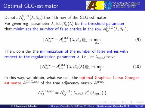
Optimal GLG-estimator

Denote AGLGi ,∗ (λ, βtr) the i-th row of the GLG estimator.

For given reg. parameter λ, let βitr(λ) be the threshold parameterthat minimizes the number of false entries in the row AGLG

i ,∗ (λ, βtr),

‖Atruei ,∗ − AGLG

i ,∗ (λ, βtr)‖1 → minβtr

. (9)

Then, consider the minimization of the number of false entries withrespect to the regularization parameter λ, i.e. let λopt,i solve


i ,∗ (λ, βitr(λ))‖1 → minλ. (10)

In this way, we obtain, what we call, the optimal Graphical Lasso Grangerestimator AGLG,opt of the true adjacency matrix Atrue:

AGLG,opti ,j = AGLG

i ,j ( λopt,i , βitr(λopt,i ) ).


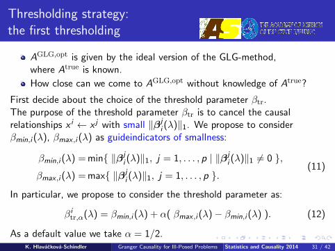
Thresholding strategy:the first thresholding

AGLG,opt is given by the ideal version of the GLG-method,where Atrue is known.

How close can we come to AGLG,opt without knowledge of Atrue?

First decide about the choice of the threshold parameter βtr.The purpose of the threshold parameter βtr is to cancel the causalrelationships x i ← x j with small ‖βj

i (λ)‖1. We propose to considerβmin,i (λ), βmax ,i (λ) as guideindicators of smallness:

βmin,i (λ) = min{ ‖βji (λ)‖1, j = 1, . . . , p | ‖βj

i (λ)‖1 6= 0 },

βmax ,i (λ) = max{ ‖βji (λ)‖1, j = 1, . . . , p }.

(11)

In particular, we propose to consider the threshold parameter as:

βitr,α(λ) = βmin,i (λ) + α( βmax ,i (λ)− βmin,i (λ) ). (12)

As a default value we take α = 1/2.K. Hlavackova-Schindler Granger Causality for Ill-Posed Problems Statistics and Causality 2014 31 / 42

Thresholding strategy:the first thresholding

The optimal GLG-estimator for each gene i with the thresholdparameter βitr,1/2 can be defined as follows.

Let λtr,1/2opt,i solve the minimization problem for each gene i :


i ,∗ (λ, βitr,1/2(λ))‖1 → minλ.

Then, the corresponding optimal GLG-estimator (i.e. for all genes)is

AGLG,opttr,1/2 (i , j) = AGLG

i ,j ( λtr,1/2opt,i , β

itr,1/2(λ

tr,1/2opt,i ) ).


The second thresholding:on the network level

The choice of the threshold parameter βitr,1/2 rises the following issue.A gene is assigned always a causal relationship, unless the solutionof ‖Y i − Xβ‖2 + λ‖β‖1 → min

β, βi (λ) is identically zero.

But how strong are these causal relationships compared to each other?The norm ‖βj

i (λ)‖1 can be seen as a strongness indicator of the causalrelationship x i ← x j .Let us now construct a matrix AGLG,opt;β

tr,1/2 , similarly to the adjacency

matrix AGLG,opttr,1/2 , where instead of 1 we put the norm ‖βj

i (λ)‖1, i.e.

AGLG,opt;βtr,1/2 (i , j) =‖βj

i (λtr,1/2opt,i )‖1 if ‖βj

i (λtr,1/2opt,i )‖1 > βitr,1/2,

AGLG,opt;βtr,1/2 (i , j) =0 otherwise.

(13)


The second thresholding:on the network level

We propose to do the thresholding on the network level similarly to thethresholding on the gene level. Define the guideindicators of smallness onthe network level:

Amin = min{ AGLG,opt;βtr,1/2 (i , j) 6= 0 },Amax = max{ AGLG,opt;β

tr,1/2 (i , j) }.

And similarly to (12), define the threshold on the network level as follows:

Atr,α1 = Amin + α1( Amax − Amin ). (14)

We call the described combination of the two thresholdings on the geneand network levels as two-level thresholding. The adjacency matrixobtained by this thresholding strategy is the following:

AGLG,opttr,1/2;α1

(i , j) =1 if AGLG,opt;βtr,1/2 (i , j) > Atr,α1 ,

AGLG,opttr,1/2;α1

(i , j) =0 otherwise.(15)


An automatic realizationof GLG-method

Case when the true adjacency matrix Atrue is not known

In addition to a thresholding strategy one needs a choice rule for theregularization parameter λ in ‖Y i − Xβ‖2 + λ‖β‖1 → min

β.

For such a choice, we propose to use the so called quasi-optimalitycriterion Tikhonov, Glasko 1965, Bauer, Reiss, 2008. One considers a setof regularization parameters

λk = λ0qk , q < 1, k = 0, 1, . . . , nλ,

and for each λk the corresponding solution of (7) βi (λk) is computed.Then, the index of the regularization parameter is selected as follows:

k iqo = argmink{ ‖βi (λk+1)− βi (λk)‖1 }. (16)


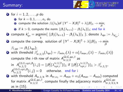
Summary:

1 for i = 1, 2, . . . , p do1 for k = 0, 1, . . . , nλ do2 compute the solution βi (λk)of ‖Y i − Xβ‖2 + λ‖β‖1 → min

β;

3 if k > 0, compute the norm ‖βi (λk+1)− βi (λk)‖1; end for k

2 compute k iqo = argmink{ ‖βi (λk+1)− βi (λk)‖1 }; denote λqo := λk i

qo;

3 compute the corresp. solution of ‖Y i − Xβ‖2 + λ‖β‖1 → minβ

βi ,qo := βi (λqo);4 with threshold βitr ,1/2(λqo) = βmin,i (λ) + α(βmax ,i (λ)− βmin,i (λ))

compute the i-th row of matrix AGLG ,qo,βtr ,1/2 as

in AGLG,opt;βtr,1/2 (i , j) = ‖βj

i (λtr,1/2opt,i )‖1 if ‖βj

i (λtr,1/2opt,i )‖1 > βitr,1/2,

AGLG,opt;βtr,1/2 (i , j) = 0 otherwise. end for i

5 with threshold Atr ,1/4 in Atr ,α1 = Amin + α1(Amax − Amin) computed

for matrix AGLG ,qo,βtr ,1/2 , compute finally the adjacency matrix AGLG ,qo

tr ,1/2;1/4

as in (15).K. Hlavackova-Schindler Granger Causality for Ill-Posed Problems Statistics and Causality 2014 36 / 42

Application: Reminder ofthe gene regulatory network

Consider a gene regulatory network of 19 genes (slide 17)

Figure : The causal structure for these genes identified by biological experimentsof Li et al. 2006.


Application and comparison

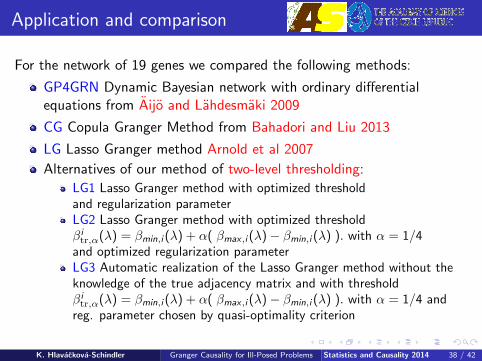
For the network of 19 genes we compared the following methods:

GP4GRN Dynamic Bayesian network with ordinary differentialequations from Aijo and Lahdesmaki 2009

CG Copula Granger Method from Bahadori and Liu 2013

LG Lasso Granger method Arnold et al 2007

Alternatives of our method of two-level thresholding:

LG1 Lasso Granger method with optimized thresholdand regularization parameterLG2 Lasso Granger method with optimized thresholdβitr,α(λ) = βmin,i (λ) + α( βmax,i (λ)− βmin,i (λ) ). with α = 1/4

and optimized regularization parameterLG3 Automatic realization of the Lasso Granger method without theknowledge of the true adjacency matrix and with thresholdβitr,α(λ) = βmin,i (λ) + α( βmax,i (λ)− βmin,i (λ) ). with α = 1/4 and

reg. parameter chosen by quasi-optimality criterion


Data and Experiments

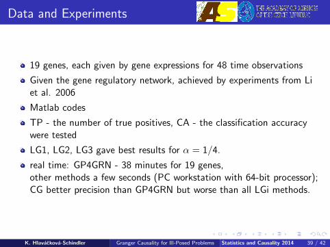
19 genes, each given by gene expressions for 48 time observations

Given the gene regulatory network, achieved by experiments from Liet al. 2006

Matlab codes

TP - the number of true positives, CA - the classification accuracywere tested

LG1, LG2, LG3 gave best results for α = 1/4.

real time: GP4GRN - 38 minutes for 19 genes,other methods a few seconds (PC workstation with 64-bit processor);CG better precision than GP4GRN but worse than all LGi methods.


Comparison

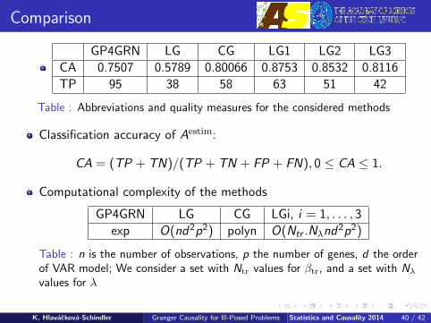
GP4GRN LG CG LG1 LG2 LG3

CA 0.7507 0.5789 0.80066 0.8753 0.8532 0.8116

TP 95 38 58 63 51 42

Table : Abbreviations and quality measures for the considered methods

Classification accuracy of Aestim:

CA = (TP + TN)/(TP + TN + FP + FN), 0 ≤ CA ≤ 1.

Computational complexity of the methods

GP4GRN LG CG LGi, i = 1, . . . , 3

exp O(nd2p2) polyn O(Ntr .Nλnd2p2)

Table : n is the number of observations, p the number of genes, d the orderof VAR model; We consider a set with Ntr values for βtr, and a set with Nλvalues for λ


Results

Figure : Causal structure from biol.experiments of Li et al. 2006.

Figure : Causal structure achieved byLasso Granger method with optim.threshold and regularization parameter


Conclusion and outlook

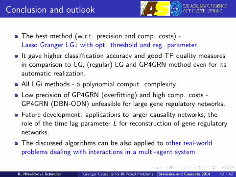
The best method (w.r.t. precision and comp. costs) -Lasso Granger LG1 with opt. threshold and reg. parameter.

It gave higher classiffication accuracy and good TP quality measuresin comparison to CG, (regular) LG and GP4GRN method even for itsautomatic realization.

All LGi methods - a polynomial comput. complexity.

Low precision of GP4GRN (overfitting) and high comp. costs -GP4GRN (DBN-ODN) unfeasible for large gene regulatory networks.

Future development: applications to larger causality networks; therole of the time lag parameter L for reconstruction of gene regulatorynetworks.

The discussed algorithms can be also applied to other real-worldproblems dealing with interactions in a multi-agent system.


granger causality for ill-posed...

Documents