This content has been downloaded from IOPscience. Please scroll down to see the full text.

Download details:

IP Address: 194.94.224.254

This content was downloaded on 15/01/2014 at 08:41

Please note that terms and conditions apply.

Gravitational wave emission from binary supermassive black holes

View the table of contents for this issue, or go to the journal homepage for more

2013 Class. Quantum Grav. 30 244009

(http://iopscience.iop.org/0264-9381/30/24/244009)

Home Search Collections Journals About Contact us My IOPscience

IOP PUBLISHING CLASSICAL AND QUANTUM GRAVITY

Class. Quantum Grav. 30 (2013) 244009 (22pp) doi:10.1088/0264-9381/30/24/244009

Gravitational wave emission from binarysupermassive black holes

A Sesana

Max-Planck-Institut fur Gravitationsphysik, Albert Einstein Institut, Am Mulenber 1,D-14476 Golm, Germany

E-mail: alberto.sesana@aei.mpg.de

Received 13 July 2013, in final form 29 October 2013Published 29 November 2013Online at stacks.iop.org/CQG/30/244009

AbstractMassive black hole binaries (MBHBs) are unavoidable outcomes of thehierarchical structure formation process, and, according to the theory of generalrelativity, are expected to be the loudest gravitational wave (GW) sources in theUniverse. In this paper I provide a broad overview of MBHBs as GW sources.After reviewing the basics of GW emission from binary systems and of MBHBformation, evolution and dynamics, I describe in some details the connectionbetween binary properties and the emitted gravitational waveform. Direct GWobservations will provide an unprecedented wealth of information about thephysical nature and the astrophysical properties of these extreme objects,allowing to reconstruct their cosmic history, dynamics and coupling with theirdense stellar and gaseous environment. In this context I describe ongoing andfuture efforts to make a direct detection with space based interferometry andpulsar timing arrays, highlighting the invaluable scientific payouts of suchenterprises.

PACS numbers: 04.70.−s, 98.65.Fz, 04.30.−w, 04.30.Db, 04.30.Tv, 04.80.Nn

(Some figures may appear in colour only in the online journal)

1. Introduction

Today, massive black holes (MBHs)1 are ubiquitous in the nuclei of nearby galaxies [1], andwe see them shining as quasars along the whole cosmic history up to redshift z ≈ 7 [2]. In thelast decade, MBHs were recognized as fundamental building blocks in hierarchical models ofgalaxy formation and evolution, but their origin remains largely unknown. In fact, our currentknowledge of the MBH population is limited to a small fraction of objects: either those thatare active, or those in our neighborhood, where stellar- and gas-dynamical measurements are

1 It is customary to use the adjective ‘supermassive’ for the 108–109 M� black holes powering quasars; conversely,we deal here with all the mass spectrum of these objects, down to their ∼103 M� seeds. We therefore refer to themgenerally as ‘massive black holes’ throughout the paper.

0264-9381/13/244009+22$33.00 © 2013 IOP Publishing Ltd Printed in the UK & the USA 1

Class. Quantum Grav. 30 (2013) 244009 A Sesana

possible. According to the current paradigm, structure formation proceeds in a hierarchicalfashion [3], in which massive galaxies grow by accreting gas through the filaments of thecosmic web and by merging with other galaxies. As a consequence, the MBHs we see intoday’s galaxies are expected to be the natural end-product of a complex evolutionary path, inwhich black holes (BHs) seeded in proto-galaxies at high redshift grow through cosmic historyvia a sequence of MBH-MBH mergers and accretion episodes [4, 5]. In this framework, a largenumber of MBH binaries (MBHBs) naturally form following the frequent galaxy mergers.

According to Einstein’s theory of general relativity (GR), accelerating masses causemodifications of the spacetime that propagate at the speed of light, better known as gravitationalwaves (GWs). However, in Einstein’s equations, the matter–metric coupling constant is of theorder of G/c4 (where G is the gravitational constant and c is the speed of light), which is∼10−50! As a matter of fact the spacetime is extraordinarily stiff, therefore only massive,compact astrophysical object can produce a sizable strain that would be observable withadvanced technology [6]. Two MBHs orbiting each other in a bound binary (MBHB) systemcarry a huge time varying quadrupole moment and are expected to be the loudest GW sourcesin the Universe [7]. The frequency spectrum of the emitted radiation covers several ordersof magnitude, from the sub-nano-Hertz up to the milli-Hertz. The 10−4–10−1 Hz windowis going to be probed by spaceborne interferometers like the recently proposed EuropeaneLISA [8–10]. At 10−9–10−7 Hz, joint precision timing of several ultrastable millisecondpulsars (i.e. a pulsar timing array, PTA) provides a unique opportunity to get the very firstlow-frequency detection. The European Pulsar Timing Array (EPTA) [11], the Parkes PulsarTiming Array (PPTA) [12] and the North American Nanohertz Observatory for GravitationalWaves (NANOGrav) [13], joining together in the International Pulsar Timing Array (IPTA)[14], are constantly improving their sensitivities, getting closer to their ambitious target.

This focus issue contribution aims at covering all the relevant aspects of MBHBs intendedas GW sources, in the spirit of providing a broad overview. Given the extent of the topic,we will just skim through its several facets, providing the appropriate references for in-depthreading. In section 2 we introduce the concept of GWs at a very basic level, defining therelevant astrophysical scales implied by MBHBs. A general overview of MBH formation andevolution (both their masses and spins), together with a brief description of MBHB dynamicsis provided in section 3. We return on GWs in section 4, where we describe in deeper detail theexpected signal from a MBHB and its dependences on the relevant parameters of the system.There, we also introduce some basics of parameter estimation theory, showing how the richastrophysical information enclosed in individual signals can be recovered. Section 5 is thendevoted to the scientific payouts of GW detection both in the milli-Hertz and in the nano-Hertzregime. We wrap-up in section 6 with some brief final remarks.

2. Gravitational waves: basics

The existence of GWs was one of the first predictions of Einstein’s GR, since they arise asnatural solutions of the linearized Einstein equations in vacuum. Expanding the metric tensoras

gμν = ημν + hμν, (1)

where ημν represent the Minkowski flat metric and ‖ hμν ‖�‖ ημν ‖, and switching to theappropriate Lorentz gauge, the perturbation hμν satisfies

� hμν = −16πG

c4Tμν, (2)

2

Class. Quantum Grav. 30 (2013) 244009 A Sesana

where � is the d’Alambertian operator and the source term Tμν is the stress–energy tensor.Equation (2) represents a set of wave equations and therefore admits wave solutions. Thesesolutions are ripples in the fabric of the spacetime propagating at the speed of light: GWs.GWs are transverse, i.e. they act in a plane perpendicular to the wave propagation, and (at leastin GR) have two distinct polarizations, usually referred to as h+ and h× (see cartoon in [6] andsection 4.2). By expanding the mass distribution of the source into multipoles, conservationlaws enforce GWs coming from the mass monopole and mass dipole to be identically zero,so that the first contribution to GW generation comes from the mass-quadrupole moment Q.The GW amplitude is therefore proportional to the second time derivative (acceleration) of Q.Moreover, energy conservation enforces the amplitude to decay as the inverse of the distanceto the source, D. A straightforward dimensional analysis shows that the amplitude of a GW isof the order of [15]

h = G

c4

1

D

d2Q

dt2. (3)

In order to generate GWs we therefore need accelerating masses with a time varying mass-quadrupole moment. The prefactor G/c4 implies that these waves are tiny, so that the onlydetectable effect is produced by massive compact astrophysical objects.

We now specialize to the case of a binary astrophysical source. From now on, weshall use Geometric units c = G = 1; in such units 1 M� = 4.927 × 10−6 s and 1pc = 9.7 × 107 s. For sources at cosmological distances (i.e., with non-negligible redshiftz), all the following equations are valid if all the masses are replaced by their redshiftedcounterparts (e.g., M → Mz = M(1+ z)), the distance D is taken to be the luminosity distance(i.e., D → DL = D(1 + z)) and f is kept to be the observed GW frequency (the frequencyin the source emission restframe is then f (1 + z)). Keeping this in mind, consider a binarysystem of masses M2 < M1, mass ratio q = M2/M1 and total mass M = M1 + M2, in circularorbit at a Keplerian frequency fK at a distance D to the observer. A detailed calculation (in thequadrupole approximation) shows that the system emits a monochromatic wave at a frequencyf = 2 fK , with inclination–polarization time averaged GW strain given by [16]:

h =√

32

5

M5/3(π f )2/3

D, (4)

where we introduced the chirp mass M = (M1M2)3/5/(M1 + M2)

1/5. For a pair ofSchwarzschild BHs, the maximum frequency of the wave is emitted at the innermost stablecircular orbit (ISCO) and can be written as:

fISCO = (π63/2M)−1, (5)

where M6 = M/106 M�. GWs carry away energy from the system, with total luminosity givenby [16]:

Lgw = dEgw

dt= 32

5(πM f )10/3. (6)

Equating the energy loss to the shrinking of the binary semimajor axis a,

1

E

dEgw

dt= −1

a

da

dt, (7)

and converting a into frequency using Kepler’s law yields

d f

dt= 64

5π8/3M5/3 f 11/3. (8)

The integral of equation (8) from f0 to fISCO defines the remaining lifetime of a binary emittingat a frequency f0 before its final coalescence.

3

Class. Quantum Grav. 30 (2013) 244009 A Sesana

Putative eccentricity plays an important role in the evolution of the binary and in theemitted GWs [17]. In this case, the luminosity at a fixed MBHB semimajor axis is boosted toLgw = Lgw,cF(e), where Lgw,c is given by equation (6) and

F(e) = (1 − e2)−7/2

(1 + 73

24e2 + 37

96e4

). (9)

Accordingly, the evolution of the binary orbit is a factor F(e) faster than in the circular case.The energy is radiated in form of a rather complicated GW spectrum, covering the spectralrange n fk, where n is an integer index (see, e.g., [18], and section 4.2 for more details). Inparticular, the emission is stronger close to the binary periastron (there, the acceleration islarger, and so is the derivative of the quadrupole moment of the source), which leads to efficientcircularization according to

de

dt= −304

15

M1M2M

a4(1 − e2)5/2e

(1 + 121

304e2

). (10)

Examples of GW driven circularization are illustrated in the MBHB evolutionary paths shownin panels ‘a3’ and ‘b3’ of figure 2.

Normalizing equation (4) to typical astrophysical MBHB values gives a strain of

h ≈ 2 × 10−18D−19 M5/3

6 f 2/3−4 , (11)

where D9 = D/109 pc and f−4 = f /10−4 Hz. If we require (somewhat arbitrarily) acoalescence timescale <T9 = T/109 yr, the integral of equation (8), together with equation (5)implies a relevant frequency range

fmin = 3.54 × 10−8T −3/89 M−5/8

6 Hz < f < fISCO = 4.4 × 10−3M−16 Hz. (12)

If we now estimate the frequency change in an observation time T as � f ≈ f T , we find

� f = 5 × 10−4M5/36 f 11/3

−4 T0 Hz, (13)

where now T0 = T/100 yr. Equations (11)–(13) define the properties of typical MBHBsignals. A light 105 M� binary spans a frequency range of 10−7 − 10−2 Hz, in a Gyrbefore the coalescence. For a source at 1 Gpc, the strain is h ≈ 2 × 10−19 at 10−3 Hz,and � f � f , implying a chirping signal rapidly sweeping through the frequency band duringa putative observation. On the other hand, a massive 109 M� binary covers a frequency rangeof 10−10 − 10−6 Hz, in a Gyr before the coalescence. For a source at 1 Gpc, the strain ish ≈ 5 × 10−16 at 10−8 Hz, and � f ≈ 10−13 Hz, implying a non-evolving, monochromaticsource. It is likely that many such sources accumulates at these low frequency, resulting inan incoherent superposition of monochromatic waves. MBHBs are therefore loud primaryGW targets in the nano-Hertz–milli-Hertz regime, and they can manifest themselves both asrapidly chirping signals (at milli-Hertz frequencies) as well as incoherent superposition ofmonochromatic waves (at nano-Hertz frequencies).

3. Massive black hole binaries

The mechanism responsible for the formation of the first seed BHs is not well understood.These primitive objects started to form at the onset of the cosmic dawn, around z ∼ 20,according to current cosmological models [19]. At an epoch of z ∼ 30 − 20, the earliest starsformed in small, metal-poor protogalactic halos may have had masses exceeding 100 M�[20], ending their lives as comparable stellar mass BHs, providing the seeds that would latergrow into MBHs [21]. However, as larger, more massive and metal enriched galactic discsprogressively formed, other paths for BH seed formation became viable (see [22] for a review).

4

Class. Quantum Grav. 30 (2013) 244009 A Sesana

Figure 1. Differential MBHB merger rate as a function of redshift for different seed formationscenarios. Adapted from [28].

Global gravitational instabilities in gaseous discs may have led to the direct formation of105 M� BH seeds [23], or to the formation of quasi-stars of 103–106 M� that later collapsedinto seed BHs [24]. Alternative scenarios are the collapse of massive stars formed in run-awaystellar collisions in young, dense star clusters [25] or the collapse of unstable self-gravitatinggas clouds in the nuclei of gas-rich galaxy mergers at later epochs [26]. Thus, the initialmass of the seeds remains one of the largest uncertainties in the present theory of MBHformation. However, once formed, these seed BHs inevitably took part in the hierarchicalstructure formation process, growing along the cosmic history through a sequence of mergersand accretion episodes [4, 5]. Figure 1 shows examples of expected MBHB merger rates as afunction of redshift for a sample of selected seed BH models ([5, 24, 27], see [29] for details).The uncertainty is large, with numbers ranging from ten to several hundreds events per year.Multiplying by the Hubble time and dividing by the number of galaxies within our Hubblehorizon (≈1011), figures imply that each galaxy experienced few to few hundred mergers inits past life, placing mergers among the crucial mechanisms in galaxy evolution.

3.1. Mass and spin evolution

Astrophysical BHs are extremely simple objects, described by two quantities only, namelytheir mass, MBH, and angular momentum, S.2 The magnitude of the latter can be expressed bythe dimensionless parameter a = S/Smax = cS/GM2

BH.3 By definition 0 � a � 1. Along thecosmic history, MBH mass and spin inevitably evolve according to three principal evolutionmechanisms: (i) merger with other MBHs, (ii) episodic accretion of compact objects, disruptedstars, or gas clouds, and (iii) prolonged accretion of large supplies of gas via accretion discs. As

2 We use boldface to express vectors and standard font to express their magnitude.3 Not to be confused with the binary semimajor axis, it will be clear case by case when we refer to one or the other.

5

Class. Quantum Grav. 30 (2013) 244009 A Sesana

Figure 2. Left panel: spin evolution of a MBH accreting incoherent packets of gas of mass 105 M�.In this experiment, a parameter F (given in each panel) defines the fraction of events in the southernhemisphere (defined with respect to the orientation of the MBH spin). N × (1−F ) accretion eventsare then isotropically distributed in the northern hemisphere, and N ×F in the southern hemisphere(F = 0.5 for an isotropic distribution on the sphere). In each panel, the black line refers to themean over 500 realizations, and red and orange shaded areas enclose intervals at 1-σ and 2-σdeviations, respectively (from [35]). Right panel: examples of MBHB evolutionary tracks in stellarenvironments [40]. Shown are the evolution of the eccentricity and binary semimajor axis in time(‘1’ and ‘2’ panels) and the evolution of the eccentricity versus the orbital frequency (‘3’ panels).In each panel we show tracks for binaries with initial eccentricity of 0.1 (solid), 0.3 (short-dashed)and 0.6 (long-dashed). The very high eccentricities achieved in the stellar driven phase imply non-negligible eccentricities in the milli-Hertz regime (probed by future space based interferometers likeeLISA, shaded area in panel ‘a3’), and potentially extremely high eccentricities in the nano-Hertzregime (targeted by PTAs, shaded area in panel ‘b3’).

shown by [29], coalescences of MBHs with random spin directions result in a broad remnantspin distribution; in particular highly spinning MBHs tend to spin-down. Despite the importantof MBH-MBH mergers, The dominant role in the mass and spin evolution of MBHs can beattribute to accretion. Continuous Eddington limited accretion implies an exponential massgrowth MBH(t) = MBH(0)exp

(1−εε

ttEdd

), where tEdd = 0.45 Gyr and ε is the mass-radiation

conversion efficiency (0.06 < ε < 0.4 for 0 < a < 1). If this happens in a coherent fashionthrough, e.g., a thin disc [30] , an initially Schwarzschild BH becomes maximally spinningafter accreting an amount of mass of the order of

√6MBH(0) [31]. However high spins imply

ε > 0.3, considerably slowing down the mass growth, making it impossible to produce a MBHof >109 M� at z = 7 (i.e. in <109 yrs). The problem is avoided if mass is accreted in a seriesof small incoherent packets (chaotic accretion [32]). In this case, depending on the angularmomentum of the accreted material, the MBH is spun up or down, performing a random walkin spin magnitude that keep it close to zero. However this is true only if the angular momentumdirection of the packets is nearly isotropically distributed on the sphere. Real galaxies usuallyshow large coherent gas structures, and a significant amount of rotation (see, e.g., [33, 34]). Ifthe spin vectors of the accreting packets have, on average, a preferential direction (i.e., theyangular momenta do not sum up to zero), then the spin evolution is more complicated, andhigh spin values might still be preferred. This is shown in the left panel of figure 2, taken from[35]. At low masses, the angular momentum of the accreted packet dominates over the MBHspin; in this case the latter always rapidly align with the former, resulting in efficient spin-up.

6

Class. Quantum Grav. 30 (2013) 244009 A Sesana

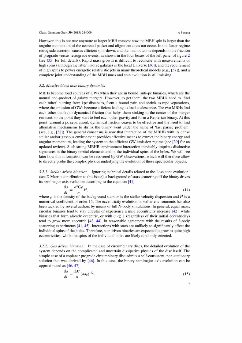
However, this is not true anymore at larger MBH masses: now the MBH spin is larger than theangular momentum of the accreted packet and alignment does not occur. In this latter regimeretrograde accretion causes efficient spin-down, and the final outcome depends on the fractionof prograde versus retrograde events, as shown in the four boxes of the left panel of figure 2(see [35] for full details). Rapid mass growth is difficult to reconcile with measurements ofhigh spins (although the latter involve galaxies in the local Universe [36]), and the requirementof high spins to power energetic relativistic jets in many theoretical models (e.g., [37]), and acomplete joint understanding of the MBH mass and spin evolution is still missing.

3.2. Massive black hole binary dynamics

MBHs become loud sources of GWs when they are in bound, sub–pc binaries, which are thenatural end-product of galaxy mergers. However, to get there, the two MBHs need to ‘findeach other’ starting from kpc distances, form a bound pair, and shrink to mpc separations,where the emission of GWs become efficient leading to final coalescence. The two MBHs findeach other thanks to dynamical friction that helps them sinking to the center of the mergerremnant, to the point they start to feel each other gravity and form a Keplerian binary. At thispoint (around a pc separation), dynamical friction ceases to be effective and the need to findalternative mechanisms to shrink the binary went under the name of ‘last parsec problem’(see, e.g., [38]). The general consensus is now that interaction of the MBHB with its densestellar and/or gaseous environment provides effective means to extract the binary energy andangular momentum, leading the system to the efficient GW emission regime (see [39] for anupdated review). Such strong MBHB–environment interaction inevitably imprints distinctivesignatures in the binary orbital elements and in the individual spins of the holes. We will seelater how this information can be recovered by GW observations, which will therefore allowto directly probe the complex physics underlying the evolution of these spectacular objects.

3.2.1. Stellar driven binaries. Ignoring technical details related to the ‘loss cone evolution’(see D Merritt contribution to this issue), a background of stars scattering off the binary drivesits semimajor axis evolution according to the equation [41]

da

dt= a2Gρ

σH, (14)

where ρ is the density of the background stars, σ is the stellar velocity dispersion and H is anumerical coefficient of order 15. The eccentricity evolution in stellar environments has alsobeen tackled by several authors by means of full N-body simulations. In general, equal mass,circular binaries tend to stay circular or experience a mild eccentricity increase [42], whilebinaries that form already eccentric, or with q � 1 (regardless of their initial eccentricity)tend to grow more eccentric [43, 44], in reasonable agreement with the results of 3-bodyscattering experiments [41, 45]. Interactions with stars are unlikely to significantly affect theindividual spins of the holes. Therefore, star driven binaries are expected to grow to quite higheccentricities, while the spins of the individual holes are likely randomly oriented.

3.2.2. Gas driven binaries. In the case of circumbinary discs, the detailed evolution of thesystem depends on the complicated and uncertain dissipative physics of the disc itself. Thesimple case of a coplanar prograde circumbinary disc admits a self-consistent, non-stationarysolution that was derived by [46]. In this case, the binary semimajor axis evolution can beapproximated as [46, 47]

da

dt= 2M

μ(aa0)

1/2. (15)

7

Class. Quantum Grav. 30 (2013) 244009 A Sesana

Here, M is the mass accretion rate at the outer edge of the disc, a0 is the semimajor axis at whichthe mass of the unperturbed disc equals the mass of the secondary MBH, and μ is the reducedmass of the binary. In the circumbinary disc scenario, eccentricity excitation has been seen inseveral simulations [48, 49]. In particular, the existence of a limiting eccentricity ecrit ≈ 0.6–0.8has been found in [50], in the case of massive self-gravitating discs. If the accretion flow iscoherent, and Ldisc and the spins Si of the two MBHs are misaligned, the Bardeen–Pettersoneffect [51] will act to align Si to Ldisc in a very short timescale (talign � tacc ∼ 108 yr [52, 53]).Therefore, in gaseous rich environments, mildly eccentric binaries might be the norm, and theMBH individual spins tend to align with the orbital angular momentum.

Compared to the GW driven case, (da/dt)gw ∝ a−3, equations (14) and (15) have a verydifferent (milder and positive) a dependence. Therefore, equating equations (14) and (15) to(da/dt)gw gives the transition frequency between the external environment driven and the GWdriven regimes. For typical astrophysical systems one gets:

fstar/GW ≈ 1.2 × 10−7M−7/106 q−3/10 Hz

fgas/GW ≈ 1.6 × 10−7M−37/496 q−69/98 Hz. (16)

Substituting M = 109 M�, we see that the transition occurs at nano-Hertz frequencies.This is the mass and frequency range of typical PTA sources, which therefore might still beinfluenced by their environment and be very eccentric (e > 0.5, see panel ‘b3’ in figure 2).Even though GW emission efficiently circularizes binaries (see section 2), low mass systems(M = 104–105 M�) decouple only at μHz frequencies and can still retain substantial residualeccentricities in the milli-Hertz window where they become eLISA targets (e > 0.01, seepanel ‘a3’ in figure 2).

4. MBHB waveforms

Having introduced the basics of GW emission from a binary system in section 2, we turnnow in some more detail to the gravitational waveform modeling. In particular we show howeccentricity and spins affect the detectable GW signal and we describe the basic theory ofinformation recovery, that enables us to dig out the parameters of the source from the detectedwaveform.

4.1. The stages of the binary coalescence

The evolution of MBHBs is customarily divided into three phases: inspiral, merger, and ring-down [55]. The inspiral is a relatively slow, adiabatic process. Different techniques have beenemployed to describe this stage, ranging from classic Post Newtonian (PN) expansions of theenergy-balance equation [56], to non-adiabatic resummed methods in which the equations ofmotion are derived from an effective one body (EOB) relativistic Hamiltonian [57]. A detaileddescription of such methods is beyond the scope of this paper, and an excellent overviewcan be found in [58]. The inspiral is followed by the dynamical coalescence, in which theMBHs plunge and merge together, forming a highly distorted, perturbed remnant. At thisstage, all analytical approximations break down, and the system can only be described bydirectly solving the Einstein equations using numerical simulations [59–61]. The distortedremnant settles into a stationary Kerr BH as it rings down, by emitting gravitational radiation.This latter stage can be, again, modeled analytically using BH perturbation theory [62]. Anexample of the full waveform with the identification of the various stages is given in figure 3.

In recent years there has been a major effort in constructing accurate waveforms inclusiveof all three phases. ‘Complete’ waveforms can be designed by stitching together analytical

8

Class. Quantum Grav. 30 (2013) 244009 A Sesana

Figure 3. Example of GW signal from two coalescing (circular, non-spinning) BHs as a functionof time. The different approximation techniques and their range of validity are indicated. Wavylines illustrate the regime close to merger where analytical methods have to be bridged by NR(courtesy of Ohme [54]).

PN waveforms for the early inspiral with a (semi)phenomenologically described merger andring-down phase calibrated against available numerical data (known as PhenomB-PhenomCwaveforms, [63]). Alternatively, complete waveforms can be constructed within the EOBformalism by adding free parameters to be calibrated against NR simulations and by attachinga series of damped sinusoidals describing the ring-down (known as EOBNR waveforms[64, 65]). A detailed overview is given in [54]. What is relevant to our discussion is thatthe full evolution of MBHBs can be tackled with a combination of analytical and numericalmethods, and accurate waveforms encoding all the parameters of the system can be computed.In the following we concentrate on the inspiral signal only, which is the richest in terms ofencoded information.

4.2. The adiabatic inspiral: impact of eccentricity and spin

Expanding the Einstein’s equations and the covariant conservation of the stress–energy tensorTμν perturbatively in powers of v/c (where v is the relative velocity of the two objects), onegets a PN series for the binary acceleration of the form [66]:

a = aN + aPN + aSO + a2PN + aSS + aRR, (17)

where aN , aPN, and a2PN are the Newtonian, (post)1-Newtonian, and (post)2-Newtoniancontributions to the equations of motion, aRR is the contribution due to the radiation-reactionforce, and aSO and aSS are the spin–orbit and spin–spin coupling contributions. In the sameway, the radiated wave (in the far field zone, see [56]) can be similarly expanded in the form:

hi j = 2μ

D

[Qi j + P0.5Qi j + PQi j + PQi j

SO + P1.5Qi j + P1.5Qi jSO + P2Qi j

SS

](18)

where Qi j is the second time derivative of the standard quadrupole moment of the source,i, j = 1, 2, 3 define the spatial components of the perturbation tensor, and the subscripts havethe same meaning as in equation (17).

A practical way to derive expressions for the acceleration and the waveform, is to employthe adiabatic approximation, in which the inspiral of the system is treated as a quasistationarysequence of orbits. For circular binaries, the evolution of the adiabatic inspiral is completelydetermined by the energy-balance equation that relates the derivative of the energy function Eto the gravitational flux F radiated away4

dE (v)

dt= −F (v) (19)

4 For eccentric binaries, an angular momentum balance equation must also be imposed to compute the evolution ineccentricity.

9

Class. Quantum Grav. 30 (2013) 244009 A Sesana

from which we may derive the binary acceleration and phase evolution as:

d

dt= 2v3

M,

dv

dt= − F (v)

MdE (v)/dv. (20)

For orbital velocities v � c, E and F can be expanded in powers of v2n to a given orderin n. Similarly, the resulting waveform is written as an expansion of the form (18), wherenow hi j do not explicitly depend on the secular adiabatic inspiral. Choosing the appropriateorthonormal radiation frame, hi j can be written as two independent polarizations only; h+and h×. Assuming a circular binary, in the adiabatic approximation, to the leading quadrupoleorder one obtains the familiar form

h+(t) = 2M5/3

D[π f (t)]2/3(1 + cos2 ι) cos (t)

h×(t) = 2M5/3

D[π f (t)]2/32 sin2 ι cos (t) (21)

where ι (usually referred as inclination) is the angle defined by the line of sight with respectto the orbital angular momentum vector, (t) = 2π

∫ t f (t ′) dt ′, and f = 2 fK as defined insection 2.

The eccentricity e enters directly in the computation of Qi j since it affects the velocityv of the MBHs along the orbit. In fact, e affects the computation of hi j at all orders, startingfrom the simple quadrupole term, by ‘splitting’ each polarization amplitude h+(t) and h×(t)into harmonics according to (see, e.g., equations (5) and (6) in [67] and references therein):

h+n (t) = A

{− (1 + cos2 ι)un(e) cos

[n

2(t) + 2γ (t)

]

−(1 + cos2 ι)vn(e) cos

[n

2(t) − 2γ (t)

]+ sin2 ιwn(e) cos

[n

2(t)

]},

h×n (t) = 2A cos ι

{un(e) sin

[n

2(t) + 2γ (t)

]+ vn(e) sin

[n

2(t) − 2γ (t)

]}. (22)

The amplitude coefficients un(e), vn(e), and wn(e) are linear combinations of the Besselfunctions of the first kind Jn(ne), Jn±1(ne) and Jn±2(ne), and γ (t) is an additional precessionterm to the phase given by e. For e � 1, |un(e)| � |vn(e)| , |wn(e)| and we recover thecircular limit given by equation (21). As GW emission tends to decrease eccentricity, this islikely to be mostly important at large separations (i.e., fK � fISCO, see panels ‘a3’ and ‘b3’in figure 2). An example of an eccentric waveform is shown in the upper panel of figure 4.

Turning now to spins, equation (17) shows that spins enter as higher order corrections(namely at the 1.5PN order, i.e. O(v/c)3) in the computation of the acceleration and,consequently, of the waveform. Therefore they become important only when v/c is large.Such corrections generate additional small terms in the phase evolution, but most importantly,cause the orbital angular momentum L to precess around the total angular momentum. At theleading order, the latter is conserved in its Newtonian form J = L + S1 + S2 (in which S1 andS2 the spins of the two MBHs) and L precesses according to the equation [68]

L =[

1

a3

(2 + 3

2q

)J]

× L (23)

(in this case a is the binary semimajor axis). The typical precession timescale is given by

Tp = L

L≈ M1/3μ−1

[2 + 3

2q

]−1

(π f )5/3 ≈ 2.5 × 103π5/3M1/36

(f

fISCO

)−5/3

(24)

10

Class. Quantum Grav. 30 (2013) 244009 A Sesana

Figure 4. Examples of waveforms from eccentric and spinning binaries. In the top panel we showa zoom-in of three wave cycles highlighting the peculiar amplitude-phase relation of a mildlyeccentric binary (e = 0.5); h+ is in red and h× is in blue. In the bottom panel we show the lastseveral thousand cycles of a spinning precessing system, the amplitude modulation given by theorbital plane precession is evident (courtesy of A Petiteau).

where we used J ≈ L, and we assumed equal mass binaries in the last equality. It is clear thatat, say, f = 10−3 fISCO, Tp is of the order of several tens of years, making precession effectsnegligible on plausible observation timescales. An example of waveform modulated by planeprecession in the late inspiral is shown in the lower panel of figure 4.

The most general detectable signal from a spinning eccentric binary is a function of 17parameters (some describing the intrinsic properties of the binary and some others related to therelative binary-detector position and orientation): two combination of the redshifted masses,M and μ;5 six parameters defining the individual spin vectors (two magnitudes a1 and a2 andfour angles); two parameters related to the eccentricity of the orbit, initial eccentricity e0 and anadditional angle defining the line of nodes; source inclination with respect to the line of sight,ι; polarization angle, ψ ; sky location, two angle usually labeled θ and φ;6 luminosity distanceDL; initial orbital phase 0; and, depending on the type of signal, initial frequency f0 or time tocoalescence tc (the two are related, in the quadrupole approximation, by equation (8)). We sawexamples of how some of these parameters are imprinted in the waveform, in the followingsubsection we turn to the problem of how accurately they can be extracted given some signalobservation.

5 As discussed in section 2, for sources at cosmological distances, the GW depends on the redshifted masses, theintrinsic ones can be extracted by measuring DL and then converting it into z according to a cosmological model, orby obtaining an independent measurement of z through, e.g., the identification of an electromagnetic counterpart tothe GW signal.6 Of particular interest is the source sky localization errorbox ��, defined, following [69], in terms of θ and φ as:�� = 2π

√(sinθ�θ�φ)2 − (sinθcθφ )2 (according to the notation used in section 4).

11

Class. Quantum Grav. 30 (2013) 244009 A Sesana

4.3. Parameter extraction

We briefly review the basic theory regarding the estimate of the statistical errors that affectthe measurements of the source parameters. For a comprehensive discussion of this topic werefer the reader to [70]. The data d collected in a detector is given by the superposition of thenoise n and a signal x determined by a vector of parameters�λ:

d(t) = n(t) + x(t;�λ). (25)

In the following, we make the usual (simplifying) assumption that n(t) is a zero-mean Gaussianand stationary random process characterized by the one-sided power spectral density Sn( f ).The inference process in which we are interested is how well one can infer the actual valueof the unknown parameter vector �λ, based on the data d, and any prior information on �λavailable before the experiment. Within the Bayesian framework, one is therefore interestedin deriving the posterior probability density function (PDF) p(�λ|d) of the unknown parametervector given the data set and the prior information. Bayes’ theorem yields

p(�λ|d) = p(�λ)p(d|�λ)

p(d), (26)

where p(d|�λ) is the likelihood function, p(�λ) is the prior probability density of�λ, and p(d) isthe marginal likelihood or evidence. Under the assumption of Gaussian noise

p(d|�λ) ≡ p[n = d − x(�λ)] ∝ exp[− 1

2 (d − x(�λ)|d − x(�λ))]

(27)

where the inner product between two functions (g|h) is defined as the integral

(g|h) = 2∫ ∞

0

g∗( f )h( f ) + g( f )h∗( f )

Sn( f )d f , (28)

applied to the Fourier transform of the functions, e.g.,

g( f ) =∫ +∞

−∞g(t) e−2π i f t . (29)

In the neighborhood of the maximum-likelihood estimate value �λ, the likelihood function canbe approximated as a multi-variate Gaussian distribution,

p(�λ|d) ∝ p(�λ) exp[− 1

2�ab�λa�λb], (30)

where �λa = λa − λa and the matrix �ab is the Fisher information matrix (FIM). Herea, b = 1, . . . , N label the components of �λ (i.e., the parameters defining the shape of thesignal), and we have used Einstein’s summation convention (and we do not distinguish betweencovariant and contravariant indices). The FIM is simply related to the derivatives of the GWsignal with respect to the unknown parameters integrated over the observation:

�ab =(

∂x(t;�λ)

∂λa

∣∣∣∣∣∂x(t;�λ)

∂λb

). (31)

In terms of the inner product (.|.) the maximal signal-to-noise ratio (SNR) at which a signalcan be observed is obtained by matched filtering of the data against a template equal to thewaveform signal, x(�λ). The optimal matched filtering SNR achievable in this way is (x|x).

In the limit of large SNR, �λ tends to �λ, and the inverse of the FIM provides a lower limitto the error covariance of unbiased estimators of �λ, the so-called Cramer–Rao bound. Thevariance–covariance matrix is simply the inverse of the FIM, and its elements are

σ 2a = (�−1)aa, cab = (�−1)ab√

σ 2a σ 2

b

, (32)

12

Class. Quantum Grav. 30 (2013) 244009 A Sesana

Figure 5. The GW landscape; total mass of the binary system versus frequency of the GWs. Theleft side shows the frequency bands of different probes: ground-based detectors, eLISA, and PTAs.The gray shaded region at the top is inaccessible because no system of a given mass can radiateat such high frequencies. The shaded region at the bottom contains detectable sources for whichthe chirp mass cannot be measured in an observation lasting less than 10 years. Sloping dottedlines show the three-year, one-day, and one-minute time-to-merger lines. Sloping dashed lines arerelevant dynamical frequencies: last stable orbit and the frequencies of ring-down modes of themerged BH. Vertical lines indicate evolutionary tracks of systems of various masses as their orbitsshrink and they move to higher frequencies: a binary neutron star (BNS), an intermediate-massbinary BH (IMBBH), and a super massive binary BH (SMBBH) (from [10]).

where −1 � cab � +1 (∀a, b) are the correlation coefficients. We can therefore interpret σ 2a as

a way to quantify the expected uncertainties on the measurements of the source parameters. Werefer the reader to [71] and references therein for an in-depth discussion of the interpretationof the inverse of the FIM in the context of assessing the prospect of the estimation of thesource parameters in GW observations. When combining α = 1, . . . , N different pieces ofindependent (i.e., having uncorrelated noise) information (for example, by observing severalpulsars, or by combining the inspiral and the ring-down portion of a signal), the FIM thatcharacterizes the joint observations in equation (30) is simply given by the sum of the matricesof all the individual pieces

�ab =∑

α

�(α)

ab , (33)

and all the theory follows unchanged.

5. The gravitational wave landscape: observations and scientific payouts

As discussed in section 2, GW emission from MBHBs covers several decades in frequency,ranging from sub-nano-Hertz to milli-Hertz. As shown in figure 5, this range is (or it will be)covered by multiple probes. The ground-based network of advanced interferometric detectors(three LIGO detectors, VIRGO [72], and the Kamioka Gravitational wave Detector, KAGRA[73]) and possibly the third-generation Einstein Telescope (ET, [74]) will observe inspirallingbinaries up to around few×100 M�. The milli-Hertz regime will be the hunting territory ofspaced based detectors such as eLISA. Acceleration noise however, will severely affect thesensitivity below 0.1 mHz, which, according to equation (5), roughly corresponds to the ISCO

13

Class. Quantum Grav. 30 (2013) 244009 A Sesana

Figure 6. Constant-contour levels of the sky and polarization angle averaged SNR for eLISA, forequal mass non-spinning binaries as a function of their total rest frame mass, M, and cosmologicalredshift, z. The tracks represent the mass-redshift evolution of selected MBHs: two possibleevolutionary paths for a MBH powering a z ≈ 6 quasar (starting from a massive seed, blue curve,or from a Pop III seed from a collapsed metal-free star, yellow curve); a typical 109 M� MBHin a giant elliptical galaxy (red curve); and a Milky Way-like MBH (green curve). Circles markMBH-MBH mergers occurring along the way [75]. The gray transparent area in the bottom rightcorner roughly identifies the parameter space for which MBHs might power phenomena that willlikely be observable by future electromagnetic probes.

of a 107 M� binary. On the other hand, PTAs start to be sensitive at 10−6 Hz (this upperlimit is set by the typical weekly cadence of millisecond pulsar observations) and extendtheir observational window all the way down to the nano-Hertz range, where inspiralling108–109 M� systems should be abundant. Therefore, space based interferometers and PTAswill provide a complementary, complete census of the MBHB population throughout theUniverse. In this section we focus on the prospects of GW observation in these two bands andon the related scientific payouts.

5.1. The milli-Hertz regime: science with space based interferometry

Space based interferometry will open a revolutionary new window on the Universe. In thefollowing we refer to the eLISA design presented in [10] to describe the extraordinary scientificpayouts of milli-Hertz GW observations. Figure 6 highlights the exquisite capabilities of eLISAin covering almost all the mass-redshift parameter space relevant to MBH astrophysics. GWobservations will catch sources with M ∼ 104 M� at early cosmological times, prior toreionization. A binary with 104 � M � 107 M� can be detected out to z ∼ 20 with aSNR � 10, making an extensive census of the MBH population in the Universe possible.

As detailed in section 4, detected waveforms carry information on all the relevant sourceparameters, including redshifted masses and spins of the individual BHs prior to coalescence,the distance to the source and its sky location. The left panel of figure 7 shows error distributionsin the source parameter estimation, for events collected in a meta-catalog of ∼1500 sources,based on state of the art MBH evolution models (see [8] for details). Here, circular precessingspinning binary were considered (i.e. waveforms determined by 15 parameters), and ‘hybrid’

14

Class. Quantum Grav. 30 (2013) 244009 A Sesana

Figure 7. Left panel: eLISA parameter estimation accuracy; meta-catalog of MBHBs described in[8]. Top panels show errors on the redshifted masses (left) and spins (right). Red solid lines are forthe primary and blue dashed lines are for the secondary MBH. The bottom panels show the errordistribution on the luminosity distance DL (left), and the sky location accuracy �� (in deg2, right).Right panel: eLISA capabilities of selecting among different MBH formation routes as a functionof observation time. Plotted is the fraction of realizations in which one of the four investigatedmodels (SE) is chosen over each of the other three models (LE (solid green), LC (long-dashedblue) and SC (short-dashed red)) at 95% confidence level, as a function of observation time. Nospin information is included.

waveforms of the PhenomC family were used to evaluate uncertainties based on the FIMapproximation, as outlined in the previous section. Individual redshifted masses can bemeasured with unprecedented precision, i.e., with an error of 0.1%–1%, on both components.The spin of the primary hole can be measured with an exquisite accuracy, to a 0.01–0.1absolute uncertainty. This precision mirrors the big imprint left by the primary MBH spin inthe waveform. The measurement is more problematic for a2 that can be either determined toan accuracy of 0.1, or remain completely undetermined, depending on the source mass ratioand spin amplitude. The source luminosity distance error has a wide spread, usually rangingfrom being undetermined (but see [76] for possible shortcomings of the FIM approximationin these cases) to a stunning few per cent accuracy (note that this is a direct measurement ofDL). GW detectors are full sky monitors, and the localization of the source in the sky is alsoencoded in the waveform pattern. Sky location accuracy is typically estimated in the range10–1000 deg2.7

While measurements of individual systems are extremely interesting and very useful formaking, e.g., strong-field tests of GR, it is the properties of the whole set of MBHB mergersthat are observed which will carry the most information for astrophysics. GW observations ofmultiple MBHBs may be used together to learn about their formation and evolution throughcosmic history, as demonstrated by [77, 78]. We briefly provide here an illustrative examplefrom [8]. As argued above, in the general picture of MBH cosmic evolution, the population isshaped by the seeding process and the accretion history. [8] therefore consider a set of fourmodels with distinctive properties: (i) small seeds and extended (coherent) accretion (SE),(ii) small seeds and chaotic accretion (SC), (iii) large seeds and extended accretion (LE),

7 These numbers assume a ‘single Michelson’ (four laser links) configuration for eLISA, the full triangular ‘twoMichelsons’ (six laser links) configuration results in a significant improvement of the estimation of all parameters, inparticular luminosity distance and sky location (by one to two orders of magnitude).

15

Class. Quantum Grav. 30 (2013) 244009 A Sesana

Table 1. Summary of all possible comparisons of the considered MBH evolution models. Resultsare for one year of observation with eLISA. We take a fixed confidence level of p = 0.95. Thenumbers in the upper-right half of each table show the fraction of realizations in which the rowmodel is chosen at more than this confidence level when the row model is true. The numbers inthe lower-left half of each table show the fraction of realizations in which the row model cannotbe ruled out at that confidence level when the column model is true. In the top table we considerthe trivariate M, q, and z distribution of observed events; in the bottom table we also include theobserved distribution of remnant spins, ar .

Without spins

SE SC LE LC

SE × 0.48 0.99 0.99SC 0.53 × 1.00 1.00LE 0.01 0.01 × 0.79LC 0.02 0.02 0.22 ×

With spins

SE SC LE LCSE × 0.96 0.99 0.99SC 0.13 × 1.00 1.00LE 0.01 0.01 × 0.97LC 0.02 0.02 0.06 ×

(iv) large seeds and chaotic accretion (LC). Each model predicts a theoretical distributionof coalescing MBHBs. A given dataset D of observed events can be compared to a givenmodel A by computing the likelihood p(D|A) that the observed dataset D is a realization ofmodel A. When testing a dataset D against a pair of models A and B, one assigns probabilitypA = p(D|A)/(p(D|A) + p(D|B)) to model A, and probability pB = 1 − pA to model B. Theprobabilities pA and pB are a measure of the relative confidence one has in model A and B,given an observation D. Setting a confidence threshold of 0.95 one can count what fractionof the 1000 realizations of model A yields a confidence pA > 0.95 when compared to analternative model B. Results are shown in the top panel of table 1 for all pairs of models,assuming one year observation and circular non-spinning waveforms (i.e., for an extremelyconservative waveform model). The majority of the pair comparisons yields a 95% confidencein the true model for almost all the realizations, with the exception of comparisons LE toLC and SE to SC, i.e., comparisons among models differing by accretion mode only. This isbecause the accretion mode (efficient versus chaotic) particularly affects the spin distributionof the coalescing systems, which is not considered in the circular non-spinning waveformmodel. It is sufficient to add a measurement of the remnant spin parameter ar to make thosepairs easily distinguishable (bottom panel of table 1). The right panel of figure 7 shows theevolution of the fraction of correctly identified models as a function of observation time (nospin information included). Small versus large seed scenarios (SE versus LE and SE versusLC) can be easily discriminated after only 1 year of observation.

5.2. The nano-Hertz regime: science with pulsar timing arrays

PTAs are sensitive at much lower frequencies (10−9 − 10−7 Hz), where the expected signalis given by a superposition of a large number of massive (M > 108 M�), relatively nearby(z < 1) sources overlapping in frequency. As argued in section 3, at such low frequencies theproperties of the MBHBs are likely to be severely affected by their coupling with their stellarand gaseous environment. In particular binaries can be highly eccentric, which might suppressthe low-frequency portion of the spectrum, crucial to PTA detection [79]. Here we consider

16

Class. Quantum Grav. 30 (2013) 244009 A Sesana

Figure 8. Left panel: simulated pulsar residuals R. The overall data, containing white noise withrms labeled in figure plus a Monte Carlo realization of the GW signal, is represented with a greenthin line; the GW signal only is given by the underlying thick red line. Right panel: Monte Carlorealization of the GW signal expected in the PTA band; characteristic amplitude versus frequency.Each cyan point represents an individual binary, and the overall signal is given by the greenspiky line. Blue filled triangles are potentially resolvable sources, and the red line is the level ofthe signal once the latter are subtracted: the unresolved background. The black solid line is theexpected analytical f −2/3 power law, and the black dashed lines represent different timing residuallevels.

circular GW driven binaries for simplicity. The overall expected characteristic strain hc of theGW signal can be written as [80]

h2c ( f ) =

∫ ∞

0dz

∫ ∞

0dM d3N

dz dM d ln fh2, (34)

where d3N/dz dM d ln f , is the comoving number of binaries emitting in a given logarithmicfrequency interval with chirp mass and redshift in the range [M,M + dM] and [z, z + dz],respectively; and h is the inclination–polarization averaged strain given by equation (4).

The GW spectrum has a characteristic shape hc = A( f /1 yr−1)−2/3, where A is the signalnormalization at f = 1 yr−1, which depends on the details of the MBH binary population only.A Monte Carlo realization of the signal is shown in figure 8 for a selected MBHB populationmodel. In the timing residual of each individual pulsar, the signal appears as a structured rednoise (left panel), but a representation of the characteristic strain in the Fourier domain revealsthe complexity of its nature (right panel). Although several millions of sources contribute to it,the bulk of the strain comes from few hundred sources only. Therefore, the signal is far frombeing a Gaussian isotropic background [87]; a handful of sources dominates the strain budget,and some of them might be individually identified. Detection techniques have been developedfor stochastic signals [88–91] and individual sources [92–94], and more sophisticated schemesaccounting for signal anisotropy have recently been proposed [95–97]. In terms of level of thestochastic signal, recent works [81, 85, 87] set a plausible range 3 × 10−16 < A < 4 × 10−15,and the newly published PPTA limit of A = 2.4 × 10−15 [84], is already digging into it.This is shown in the left panel of figure 9, where observations are compared to theoreticallypredictions. Here, the difference between the top-left and the top-right panels is given bythe recent upgrades in the MBH mass–host relation [98, 99] to include the overmassive BHsmeasured in brightest cluster galaxies (BCGs) [100], that boost-up the range of expectedsignals by a factor of 2. In the lower panels instead, we consider two subset of the models

17

Class. Quantum Grav. 30 (2013) 244009 A Sesana

Figure 9. Left panel: characteristic amplitude of the GW signal. Shaded areas represent the 68%,95% and 99.7% confidence levels given by [81]. In each panel, the asterisks mark the limits givenby NANOGrav[82] (magenta), the EPTA [83] (black), and the PPTA [84] (red). Shaded areas inthe upper left panel refer to the 95% confidence level given by [85] (red) and the uncertainty rangeestimated by [80] (black). Right panel: median expected statistical error on the source parameters.Each point (asterisk or square) is obtained by averaging over a large Monte Carlo sample ofMBHBs. In each panel, solid lines (squares) represent the median statistical error as a function ofthe total coherent SNR, assuming 100 randomly distributed pulsars in the sky; the thick dashedlines (asterisks) represent the median statistical error as a function of the number of pulsars for afixed total SNR = 10. In this latter case, thin dashed lines label the 25th and the 75th percentile ofthe error distributions (from [86]).

featuring these upgraded relations: (i) those in which accretion does not occur prior to binarycoalescence, and (ii) those in which accretion precedes the formation of the binary, and ismore prominent on the secondary MBH [101]. In the latter case, binaries observed by PTA aremuch more massive (and have larger mass ratios) implying a much larger (by almost a factorof 3) signal. Although the PPTA limit is already ruling out some of the models, we must stressonce again that the assumption of circular GW driven binaries might not hold [102], whichmight lead to the partial suppression of the low-frequency signal [79]. Therefore, drawingconclusions about the population of MBHBs from the current limits is not a straightforwardtask.

An handful of sources might be bright enough to be individually resolved, and in thiscase some of their parameters can be determined according to the scheme described insection 4. A pioneering investigation was performed by [86] assuming circular, non-spinningmonochromatic systems. In this case the waveform is function of seven parameters only:the amplitude R,8 sky location θ, φ, polarization ψ , inclination ι, frequency f and phase0, defining the parameter vector�λ = {R, θ, φ, ψ, ι, f ,0}. Results about typical parameterestimation accuracy are shown in the right panel of figure 9 for a detection SNR = 10. Thesource amplitude is determined to a 20% accuracy, whereas φ,ψ, ι are only determined withina fraction of a radian. Sky location within few tens to few deg2 is possible (see also [92, 94]),and even sub deg2 determination, under some specific conditions [103]. Even though this isa large chunk of the sky, these systems are extremely massive and at relatively low redshift(z < 0.5), making any putative electromagnetic signature of their presence (e.g., emissionperiodicity related to the binary orbital period, peculiar emission spectra, peculiar Kα lineprofiles, etc) detectable [104, 105].8 For monochromatic signals the two masses and the luminosity distance degenerate into a single amplitude parameter.

18

Class. Quantum Grav. 30 (2013) 244009 A Sesana

6. Conclusions

We provided a general overview of massive black hole binaries (MBHBs) as gravitationalwave (GW) sources. MBHs are today ubiquitous in massive galaxies, and power luminousquasars up to z > 7. Although they are believed to play a central role in the process ofstructure formation, their origin and early growth is largely unknown. According to our currentunderstanding, MBHBs must form in large numbers along the cosmic history, providing theloudest sources of GWs in the Universe in a wide range of frequencies spanning from thesub-nano-Hertz up to the milli-Hertz. GWs carry precise information about the parametersof the emitting systems. We showed how those parameters are imprinted in the phase (andamplitude) modulation of the wave, and can therefore be efficiently extracted and determinedto high accuracy with ongoing and future GW probes. From those we will learn about MBHformation and evolution through cosmic history, about the nature of the first black hole (BH)seeds, their subsequent accretion history, and, more generally, about the early hierarchicalstructure formation at high redshift. We will also learn about the complex interplay of physicalprocesses, including stellar and gas dynamics and GW emission, that leads to the dynamicalformation and evolution of MBHBs. Direct GW detection will open a new era in MBH andMBHB astrophysics.

Acknowledgments

I would like to thank S Babak, M Dotti, F Ohme and A Petiteau for providing useful material,and E Barausse for useful discussions about the PN formalism. This work is supported by theDFG grant SFB/TR 7 Gravitational Wave Astronomy and by DLR (Deutsches Zentrum furLuft- und Raumfahrt).

References

[1] Magorrian J et al 1998 The demography of massive dark objects in galaxy centers Astron. J. 115 2285–305[2] Mortlock D J et al 2011 A luminous quasar at a redshift of z = 7.085 Nature 474 616–9[3] White S D M and Rees M J 1978 Core condensation in heavy halos: a two-stage theory for galaxy formation

and clustering Mon. Not. R. Astron. Soc. 183 341–58[4] Kauffmann G and Haehnelt M 2000 A unified model for the evolution of galaxies and quasars Mon. Not. R.

Astron. Soc. 311 576–88[5] Volonteri M, Haardt F and Madau P 2003 The assembly and merging history of supermassive black holes in

hierarchical models of galaxy formation Astrophys. J. 582 559–73[6] Thorne K S 1995 Gravitational waves Particle and Nuclear Astrophysics and Cosmology in the Next Millennium

ed E W Kolb and R D Peccei (Singapore: World Scientific) p 160[7] Hughes S A 2002 Untangling the merger history of massive black holes with LISA Mon. Not. R. Astron.

Soc. 331 805–16[8] Amaro-Seoane P et al 2013 eLISA: astrophysics and cosmology in the millihertz regime GW Notes 6 4–110[9] Amaro-Seoane P et al 2012 Low-frequency gravitational-wave science with eLISA/NGO Class. Quantum

Grav. 29 124016[10] Amaro-Seoane P et al 2013 The gravitational universe arXiv:1305.5720[11] Ferdman R D et al 2010 The European pulsar timing array: current efforts and a LEAP toward the future Class.

Quantum Grav. 27 084014[12] Manchester R N et al 2012 The Parkes pulsar timing array project arXiv:1210.6130[13] Jenet F A et al 2009 The North American nanohertz observatory for gravitational waves arXiv:0909.1058[14] Hobbs G et al 2010 The international pulsar timing array project: using pulsars as a gravitational wave detector

Class. Quantum Grav. 27 084013[15] Hughes S A 2003 Listening to the Universe with gravitational-wave astronomy Ann. Phys. 303 142–78[16] Thorne K S 1987 Gravitational radiation Three Hundred Years of Gravitation (Cambridge: Cambridge

University Press) pp 330–458

19

Class. Quantum Grav. 30 (2013) 244009 A Sesana

[17] Peters P C and Mathews J 1963 Gravitational radiation from point masses in a Keplerian orbit Phys.Rev. 131 435–40

[18] Pierro V, Pinto I M, Spallicci A D, Laserra E and Recano F 2001 Fast and accurate computational tools forgravitational waveforms from binary stars with any orbital eccentricity Mon. Not. R. Astron. Soc. 325 358–72

[19] Tegmark M, Silk J, Rees M J, Blanchard A, Abel T and Palla F 1997 How small were the first cosmologicalobjects? Astrophys. J. 474 1

[20] Bromm V, Coppi P S and Larson R B 1999 Forming the first stars in the Universe: the fragmentation ofprimordial gas Astrophys. J. Lett. 527 L5–L8

[21] Madau P and Rees M J 2001 Massive black holes as population III remnants Astrophys. J. Lett. 551 L27–30[22] Volonteri M 2010 Formation of supermassive black holes Astron. Astrophys. Rev. 18 279–315[23] Koushiappas S M, Bullock J S and Dekel A 2004 Massive black hole seeds from low angular momentum

material Mon. Not. R. Astron. Soc. 354 292–304[24] Begelman M C, Volonteri M and Rees M J 2006 Formation of supermassive black holes by direct collapse in

pre-galactic haloes Mon. Not. R. Astron. Soc. 370 289–98[25] Devecchi B and Volonteri M 2009 Formation of the first nuclear clusters and massive black holes at high

redshift Astrophys. J. 694 302–13[26] Mayer L, Kazantzidis S, Escala A and Callegari S 2010 Direct formation of supermassive black holes via

multi-scale gas inflows in galaxy mergers Nature 466 1082–4[27] Koushiappas S M and Zentner A R 2006 Testing models of supermassive black hole seed formation through

gravity waves Astrophys. J. 639 7–22[28] Sesana A, Volonteri M and Haardt F 2007 The imprint of massive black hole formation models on the LISA

data stream Mon. Not. R. Astron. Soc. 377 1711–6[29] Hughes S A and Blandford R D 2003 Black hole mass and spin coevolution by mergers Astrophys. J.

Lett. 585 L101–4[30] Shakura N I and Sunyaev R A 1973 Black holes in binary systems. Observational appearance Astron. Astrophys.

24 337–55[31] Thorne K S 1974 Disk-accretion onto a black hole: II. Evolution of the hole Astrophys. J. 191 507–20[32] King A R, Lubow S H, Ogilvie G I and Pringle J E 2005 Aligning spinning black holes and accretion discs

Mon. Not. R. Astron. Soc. 363 49–56[33] Kassin S A et al 2012 The epoch of disk settling: z∼ 1 to now Astrophys. J. 758 106[34] Fabricius M H, Saglia R P, Fisher D B, Drory N, Bender R and Hopp U 2012 Kinematic signatures of bulges

correlate with bulge morphologies and Sersic index Astrophys. J. 754 67[35] Dotti M, Colpi M, Pallini S, Perego A and Volonteri M 2013 On the orientation and magnitude of the black

hole spin in galactic nuclei Astrophys. J. 762 68[36] Reynolds C S 2013 Measuring black hole spin using x-ray reflection spectroscopy arXiv:1302.3260[37] Blandford R D and Znajek R L 1977 Electromagnetic extraction of energy from Kerr black holes Mon. Not.

R. Astron. Soc. 179 433–56[38] Milosavljevic M and Merritt D 2003 Long-term evolution of massive black hole binaries Astrophys.

J. 596 860–78[39] Dotti M, Sesana A and Decarli R 2012 Massive black hole binaries: dynamical evolution and observational

signatures Adv. Astron. 2012 940568[40] Sesana A 2010 Self consistent model for the evolution of eccentric massive black hole binaries in stellar

environments: implications for gravitational wave observations Astrophys. J. 719 851–64[41] Quinlan G D 1996 The dynamical evolution of massive black hole binaries: I. Hardening in a fixed stellar

background New Astron. 1 35–56[42] Merritt D, Mikkola S and Szell A 2007 Long-term evolution of massive black hole binaries: III. Binary

evolution in collisional nuclei Astrophys. J. 671 53–72[43] Matsubayashi T, Makino J and Ebisuzaki T 2007 Orbital evolution of an IMBH in the galactic nucleus with a

massive central black hole Astrophys. J. 656 879–96[44] Preto M, Berentzen I, Berczik P and Spurzem R 2011 Fast coalescence of massive black hole binaries from

mergers of galactic nuclei: implications for low-frequency gravitational-wave astrophysics Astrophys. J.Lett. 732 L26

[45] Sesana A, Haardt F and Madau P 2006 Interaction of massive black hole binaries with their stellar environment:I. Ejection of hypervelocity stars Astrophys. J. 651 392–400

[46] Ivanov P B, Papaloizou J C B and Polnarev A G 1999 The evolution of a supermassive binary caused by anaccretion disc Mon. Not. R. Astron. Soc. 307 79–90

[47] Haiman Z, Kocsis B and Menou K 2009 The population of viscosity- and gravitational wave-drivensupermassive black hole binaries among luminous active galactic nuclei Astrophys. J. 700 1952–69

20

Class. Quantum Grav. 30 (2013) 244009 A Sesana

[48] Armitage P J and Natarajan P 2005 Eccentricity of supermassive black hole binaries coalescing from gas-richmergers Astrophys. J. 634 921–7

[49] Cuadra J, Armitage P J, Alexander R D and Begelman M C 2009 Massive black hole binary mergers withinsubparsec scale gas discs Mon. Not. R. Astron. Soc. 393 1423–32

[50] Roedig C, Dotti M, Sesana A, Cuadra J and Colpi M 2011 Limiting eccentricity of subparsec massive blackhole binaries surrounded by self-gravitating gas discs Mon. Not. R. Astron. Soc. 415 3033–41

[51] Bardeen J M and Petterson J A 1975 The Lense–Thirring effect and accretion disks around Kerr black holesAstrophys. J. Lett. 195 L65

[52] Scheuer P A G and Feiler R 1996 The realignment of a black hole misaligned with its accretion disc Mon. Not.R. Astron. Soc. 282 291

[53] Perego A, Dotti M, Colpi M and Volonteri M 2009 Mass and spin co-evolution during the alignment of a blackhole in a warped accretion disc Mon. Not. R. Astron. Soc. 399 2249–63

[54] Ohme F 2012 Analytical meets numerical relativity: status of complete gravitational waveform models forbinary black holes Class. Quantum Grav. 29 124002

[55] Flanagan E E and Hughes S A 1998 Measuring gravitational waves from binary black hole coalescences: I.Signal to noise for inspiral, merger, and ringdown Phys. Rev. D 57 4535–65

[56] Blanchet L 2006 Gravitational radiation from post-Newtonian sources and inspiralling compact binaries LivingRev. Rel. 9 4

[57] Buonanno A and Damour T 1999 Effective one-body approach to general relativistic two-body dynamics Phys.Rev. D 59 084006

[58] Buonanno A, Chen Y and Vallisneri M 2003 Detecting gravitational waves from precessing binaries of spinningcompact objects: adiabatic limit Phys. Rev. D 67 104025

[59] Pretorius F 2005 Evolution of binary black-hole spacetimes Phys. Rev. Lett. 95 121101[60] Campanelli M, Lousto C O, Marronetti P and Zlochower Y 2006 Accurate evolutions of orbiting black-hole

binaries without excision Phys. Rev. Lett. 96 111101[61] Baker J G, Centrella J, Choi D-I, Koppitz M and van Meter J 2006 Gravitational-wave extraction from an

inspiraling configuration of merging black holes Phys. Rev. Lett. 96 111102[62] Berti E, Cardoso V and Will C M 2006 Gravitational-wave spectroscopy of massive black holes with the space

interferometer LISA Phys. Rev. D 73 064030[63] Santamarıa L et al 2010 Matching post-Newtonian and numerical relativity waveforms: systematic errors and

a new phenomenological model for nonprecessing black hole binaries Phys. Rev. D 82 064016[64] Damour T, Nagar A, Hannam M, Husa S and Brugmann B 2008 Accurate effective-one-body waveforms of

inspiralling and coalescing black-hole binaries Phys. Rev. D 78 044039[65] Buonanno A, Pan Y, Pfeiffer H P, Scheel M A, Buchman L T and Kidder L E 2009 Effective-one-body

waveforms calibrated to numerical relativity simulations: coalescence of nonspinning, equal-mass blackholes Phys. Rev. D 79 124028

[66] Kidder L E 1995 Coalescing binary systems of compact objects to (post)5/2-Newtonian order: V. Spin effectsPhys. Rev. D 52 821–47

[67] Willems B, Vecchio A and Kalogera V 2008 Probing white dwarf interiors with LISA: peri astron precessionin eccentric double white dwarfs Phys. Rev. Lett. 100 041102

[68] Vecchio A 2004 LISA observations of rapidly spinning massive black hole binary systems Phys. Rev.D 70 042001

[69] Cutler C 1998 Angular resolution of the LISA gravitational wave detector Phys. Rev. D 57 7089–102[70] Jaynes E T and Bretthorst G L 2003 Probability Theory (Cambridge: Cambridge University Press)[71] Vallisneri M 2008 Use and abuse of the Fisher information matrix in the assessment of gravitational-wave

parameter-estimation prospects Phys. Rev. D 77 042001[72] Aasi J et al 2013 Search for gravitational waves from binary black hole inspiral, merger, and ringdown in

LIGO-virgo data from 2009–2010 Phys. Rev. D 87 022002[73] Somiya K 2012 Detector configuration of KAGRA—the Japanese cryogenic gravitational-wave detector Class.

Quantum Grav. 29 124007[74] Punturo M et al 2010 The Einstein telescope: a third-generation gravitational wave observatory Class. Quantum

Grav. 27 194002[75] Volonteri M and Natarajan P 2009 Journey to the MBH -σ relation: the fate of low-mass black holes in the

Universe Mon. Not. R. Astron. Soc. 400 1911–8[76] Sesana A 2013 detecting massive black hole binaries and unveiling their cosmic history with gravitational

wave observations 9th LISA Symposium (Astronomical Society of the Pacific Conference Series vol 467)ed G Auger, P Binetruy and E Plagnol (San Francisco, CA: ASP) p 103

[77] Plowman J E, Hellings R W and Tsuruta S 2011 Constraining the black hole mass spectrum with gravitationalwave observations: II. Direct comparison of detailed models Mon. Not. R. Astron. Soc. 415 333–52

21

Class. Quantum Grav. 30 (2013) 244009 A Sesana

[78] Sesana A, Gair J, Berti E and Volonteri M 2011 Reconstructing the massive black hole cosmic history throughgravitational waves Phys. Rev. D 83 044036

[79] Sesana A 2013 Insights on the astrophysics of supermassive black hole binaries from pulsar timing observationsMon. Not. R. Astron. Soc. 433 L1–L5

[80] Sesana A, Vecchio A and Colacino C N 2008 The stochastic gravitational-wave background from massiveblack hole binary systems: implications for observations with pulsar timing arrays Mon. Not. R. Astron.Soc. 390 192–209

[81] Sesana A 2013 Systematic investigation of the expected gravitational wave signal from supermassive blackhole binaries in the pulsar timing band Mon. Not. R. Astron. Soc. 433 L1–5

[82] Demorest P B et al 2013 Limits on the stochastic gravitational wave background from the North AmericanNanohertz Observatory for gravitational waves Astrophys. J. 762 94

[83] van Haasteren R et al 2011 Placing limits on the stochastic gravitational-wave background using Europeanpulsar timing array data Mon. Not. R. Astron. Soc. 414 3117–28

[84] Shannon R M et al 2013 Gravitational-wave limits from pulsar timing constrain supermassive black holeevolution Science 342 334–7

[85] McWilliams S T, Ostriker J P and Pretorius F 2012 Gravitational waves and stalled satellites from massivegalaxy mergers at z � 1 arXiv:1211.5377

[86] Sesana A and Vecchio A 2010 Measuring the parameters of massive black hole binary systems with pulsartiming array observations of gravitational waves Phys. Rev. D 81 104008

[87] Ravi V, Wyithe J S B, Hobbs G, Shannon R M, Manchester R N, Yardley D R B and Keith M J 2012 Does a‘stochastic’ background of gravitational waves exist in the pulsar timing band? Astrophys. J. 761 84

[88] Hellings R W and Downs G S 1983 Upper limits on the isotropic gravitational radiation background frompulsar timing analysis Astrophys. J. Lett. 265 L39–42

[89] Jenet F A, Hobbs G B, Lee K J and Manchester R N 2005 Detecting the stochastic gravitational wavebackground using pulsar timing Astrophys. J. Lett. 625 L123–6

[90] van Haasteren R, Levin Y, McDonald P and Lu T 2009 On measuring the gravitational-wave background usingpulsar timing arrays Mon. Not. R. Astron. Soc. 395 1005–14

[91] Anholm M, Ballmer S, Creighton J D E, Price L R and Siemens X 2009 Optimal strategies for gravitationalwave stochastic background searches in pulsar timing data Phys. Rev. D 79 084030

[92] Ellis J A, Siemens X and Creighton J D E 2012 Optimal strategies for continuous gravitational wave detectionin pulsar timing arrays Astrophys. J. 756 175

[93] Babak S and Sesana A 2012 Resolving multiple supermassive black hole binaries with pulsar timing arraysPhys. Rev. D 85 044034

[94] Petiteau A, Babak S, Sesana A and de Araujo M 2013 Resolving multiple supermassive black hole binarieswith pulsar timing arrays: II. Genetic algorithm implementation Phys. Rev. D 87 064036

[95] Cornish N J and Sesana A 2013 Pulsar timing array analysis for black hole backgrounds Class. QuantumGrav. 30 224005

[96] Mingarelli C M F, Sidery T, Mandel I and Vecchio A 2013 Characterising gravitational wave stochasticbackground anisotropy with pulsar timing arrays Phys. Rev. D 88 062005

[97] Taylor S R and Gair J R 2013 Searching for anisotropic gravitational-wave backgrounds using pulsar timingarrays Phys. Rev. D 88 084001

[98] McConnell N J and Ma C-P 2013 Revisiting the scaling relations of black hole masses and host galaxyproperties Astrophys. J. 764 184

[99] Graham A W and Scott N 2013 The M BH-L spheroid relation at high and low masses, the quadratic growth ofblack holes, and intermediate-mass black hole candidates Astrophys. J. 764 151

[100] Hlavacek-Larrondo J, Fabian A C, Edge A C and Hogan M T 2012 On the hunt for ultramassive black holesin brightest cluster galaxies Mon. Not. R. Astron. Soc. 424 224–31

[101] Callegari S, Kazantzidis S, Mayer L, Colpi M, Bellovary J M, Quinn T and Wadsley J 2011 Growing massiveblack hole pairs in minor mergers of disk galaxies Astrophys. J. 729 85

[102] Roedig C and Sesana A 2012 Origin and implications of high eccentricities in massive black hole binaries atsub-pc scales J. Phys.: Conf. Ser. 363 012035

[103] Lee K J, Wex N, Kramer M, Stappers B W, Bassa C G, Janssen G H, Karuppusamy R and Smits R2011 Gravitational wave astronomy of single sources with a pulsar timing array Mon. Not. R. Astron.Soc. 414 3251–64

[104] Sesana A, Roedig C, Reynolds M T and Dotti M 2012 Multimessenger astronomy with pulsar timing and x-rayobservations of massive black hole binaries Mon. Not. R. Astron. Soc. 420 860–77

[105] Tanaka T, Menou K and Haiman Z 2011 Electromagnetic counterparts of supermassive black hole binariesresolved by pulsar timing arrays Mon. Not. R. Astron. Soc. 420 705–19

22