greenhouse gas emissions from pig and chicken supply ... · bpex. 2010. 2009 pig cost of production...

75

References

Ajala, M.K., Adeshinwa, A.O.K. & Mohammed, A.K. 2007. Characteristics of smallholder pig production in southern Kaduna area of Kaduna State, Nigeria. American-Eurasian J. Agric. & Environ. Science, 2(2): 182–188.

Basset-Mens, C., van der Werf, H.M.G., Durand, P. & Leterme, P. 2004. Implica-tions of uncertainty and variability in the life cycle assessment of pig farming sys-tems. International Environmental Modelling and Software Society iEMSs 2004 International Conference.

Basset-Mens, C. & van der Werf, H.M.G. 2005. Scenario-based environmental as-sessment of farming systems: the case of pig production in France. Agriculture, Ecosystems and Environment, 105: 127–144.

BPEX. 2010. 2009 Pig cost of production in selected countries. Agriculture and Horticulture Development Board. Stoneleigh Park, UK.

BSI. 2008. PAS 2050:2008. Specification for the assessment of the life cycle green-house gas emissions of goods and services. British Standards Institution, UK.

Cederberg, C. & Flysjö, A. 2004. Environmental assessment of future pig farming systems - quantifications of three scenarios from the FOOD 21 synthesis work. The Swedish Institute for Food and Biotechnology, SIK report No. 723: 1–54.

Cederberg, C., Sonesson, U., Henriksson, M., Sund, V. & Davis, J. 2009. Green-house gas emissions from Swedish production of meat, milk and eggs from 1990 and 2005. The Swedish Institute for Food and Biotechnology, SIK report No. 793.

Cederberg, C. & Stadig, M. 2003. System expansion and allocation in life cycle assessment of milk and beef production, Int. J. Life Cycle Assess. 8(6):350–356.

Cooper, O. 2010. Poultry sector relies more on specialists to meet NVZ rules. Farmers’ Weekly 18/1/2010.

Dalgaard, R. 2007. The environmental impact of pork production from a life cycle perspective. University of Aarhus and Aalborg University. (Ph.D. thesis)

Dämmgen, U., Brade, W., Schulz, J., Kleine Klausing, H., Hutchings, N.J., Hae-nel, H.-D. & Rösemann, C. 2011. The effect of feed composition and feeding strategies on excretion rates in German pig production. Forestry Research 4(61): 327–342.

Dekker, S.E.M., de Boer, I.J.M., Arnink, A.J.A. & Groot, K. 2008. Environmen-tal hotspot identification of organic egg production. In Towards a sustainable management of the food chain, proceedings of the 6th International Conference on the life cycle assessment in the agri-food sector. Zurich, Switzerland, 12–14 November 2008, pp. 381–389.

Dunkley, C.S., Cunningham, D.L. & Harris, G.H. 2011. The value of poultry lit-ter in South Georgia. UGA Cooperative Extension Bulletin, 1386.

EEA. 2007. Annual European Community greenhouse gas inventory 1990–2005 and inventory report 2007 submission to the UNFCCC Secretariat version 27 May 2007.

Eriksson, I.S., Elmquist, H., Stern, S. & Nybrant, T. 2005. Environmental sys-tems analysis of pig production - the impact of feed choice. International Jour-nal of LCA, 10(2): 143–154.

76

Greenhouse gas emissions from pig and chicken supply chains

FAO. 2004. Small scale poultry production, by Sonaiya, E. B. & Swan, S.E.J. FAO, Rome.

FAO. 2006. Livestock’s long shadow – Environmental issues and options, by Stein-feld, H., Gerber, P., Wassenaar, T., Castel, V., Rosales, M. & de Haan, C. FAO, Rome.

FAO. 2007. Gridded livestock of the world 2007 by Wint, W. and Robinson, T. Rome, FAO.

FAO. 2010. Greenhouse gas emissions from the dairy sector – A life cycle assessment, by. Gerber, P., Vellinga, T., Opio, C., Henderson, B. & Steinfeld, H. FAO, Rome.

Steinfeld, H. Mooney, A., Schneider, F. & L. E. Neville. Livestock in a changing landscape. Drivers, consequences and responses. Island Press, Washington DC.

FAO. 2011. Global livestock production systems, by T. P. Robinson, Thornton, P.K., Franceschini, G., Kruska, R.L., Chiozza, F., Notenbaert, A., Cecchi, G., Her-rero, M., Epprecht, M., Fritz, S., You, L., Conchedda, G. & See, L. FAO, Rome.

FAO. 2013a. Tackling climate change through livestock, by Gerber, P., Steinfeld, H., Henderson, B., Opio, C., Mottet, A., Dijkman, J., Falcucci, A. & Tempio, G. FAO, Rome.

FAO. 2013b. Greenhouse gas emissions from ruminant supply chains – A life cycle assessment, by Opio, C., Gerber, P., Mottet, A., Falcucci, A., Tempio, G., Ma-cLeod, M., Vellinga, T., Henderson, B. & Steinfeld, H. FAO, Rome.

Flysjö, A., Cederberg, C & Strid, I. 2008. LCA-databas för konventionella foder-medel - miljöpåverkan i samband med production. SIK rapport No. 772, Version 1.1.

FOE. 2010. Pastures new: a sustainable future for meat and dairy farming. Friends of Earth, London.

Guy, J. H., Rowlinson, P., Chadwick, J.P. & Ellis, M. 2002. Growth performance and carcass characteristics of two genotypes of growing-finishing pig in three different housing systems. Animal Science, 74(3): 493–502.

Halberg, N., Hermansen, J.E., Kristensen, I.S., Eriksen, J., Tvedegaard, N. & Pe-tersen, B.M. 2010. Impact of organic pig production systems on CO2 emission, C sequestration and nitrate pollution. Agronomy for Sustainable Development, 30: 721–731.

Hijmans, R.J., Cameron, S.E., Parra, J.L., Jones P.G. & Jarvis A. 2005. Very high resolution interpolated climate surfaces for global land areas. International Jour-nal of Climatology 25(15): 1965-1978.

IPCC. 1997. Revised 1996 IPCC guidelines for national greenhouse inventories. Houghton, J.T., Meira Filho, L.G., Lim, B., Tréanton, K., Mamaty, I., Bonduki, Y., Griggs, D.J. & Callander, B.A. eds. IPCC/OECD/IEA, Paris.

IPCC. 2000. IPCC Good practice guidance and uncertainty management in na-tional greenhouse gas inventories. IPCC National Greenhouse Cost Inventories Programme, Technical Support Unit.

IPCC. 2006. 2006 IPCC Guidelines for National Greenhouse Gas Inventories, pre-pared by the National Greenhouse Gas Inventories Programme, Eggleston H.S., Buendia L., Miwa K., Ngara T. and Tanabe K. (eds). IGES, Japan.

ISO. 2006a. Environmental management—life cycle assessment: principles and framework. ISO14040, Geneva.

ISO. 2006b. Environmental management—life cycle assessment: requirements and guidelines. ISO14044, Geneva.

77

References

Jeroch, H. 2011. Recommendations for energy and nutrients of layers: a critical review. Lohmann Information 46(2): 61–72.

Kyriazakis. I. 2011. Opportunities to improve nutrient efficiency in pigs and poul-try through breeding. Animal, 5(6): 821–832.

Kool, A., Blonk, H., Ponsioen, T., Sukkel, W., Vermeer, H., de Vries, J. & Hoste, R. 2009. Carbon footprints of conventional and organic pork assessment of typi-cal production systems in the Netherlands, Denmark, England and Germany. Gouda, Blonk Milieuadvies/WUR.

Leinonen, I., Williams, A.G., Wiseman, J., Guy, J., Kyriazakis, I. 2012a. Predicting the environmental impacts of chicken systems in the United Kingdom through a life-cycle assessment: broiler production systems. Poultry Sci., 91(1): 8–25.

Leinonen, I., Williams, A.G., Wiseman, J., Guy, J. & Kyriazakis, I. 2012b. Pre-dicting the environmental impacts of chicken systems in the United Kingdom through a life-cycle assessment: egg production systems. Poultry Sci., 91(1): 26–40.

Lemke, U., Kaufmann, B., Thuy, L.T. Emrich, K. & Valle Zárate, A. 2006. Evalu-ation of smallholder pig production systems in North Vietnam: pig production management and pig performances. Livestock Science, 105: 229–243,

Lesschen, J.P., van den Berg, M., Westhoek, H.J., Witzke, H.P. & Oenema, O. 2011. Greenhouse gas emission profiles of European livestock sectors. Anim. Feed Sci. Technol., 1628: 166–177.

Lory, J., Massey, R.E. & Zulovich, J.M. 2009. An evaluation of the USEPA calcula-tions of greenhouse gas emissions from anaerobic lagoons. Journal of environ-mental quality, 39(3): 776–83.

Mkhabela, T.S. 2004. Substitution of fertiliser with poultry manure: is this eco-nomically viable? Agrekon, 43(3): 347–356.

Mollenhorst, H., Berentsen, P.B.M. & De Boer, I.J.M. 2006. On-farm quantifica-tion of sustainability indicators: an application to egg production systems, Brit-ish Poultry Science, 47(4): 405–417.

Nielsen, N., Jørgensen, M. & Bahrndorff, S. 2011. Greenhouse gas emission from the Danish broiler production estimated via LCA methodology. AgroTech/Knowledge Centre for Agriculture. Aarhus, Danemark.

Pelletier, N. 2008. Environmental performance in the US broiler poultry sector. Agricultural Systems, 98: 67–73.

Pelletier, N. Lammers, O.P., Stender, D. & Pirog, R. 2010. Life cycle assessment of high- and low-profitability commodity and deep-bedded niche swine produc-tion systems in the upper midwestern United States. Agricultural Systems, 103: 599–608.

Petri, A. & Lemme, A. 2007. Trends and latest issues in broiler diet formulation, Lohmann Information, 42(2): 25–37

Prudêncio da Silva, V., van der Werf, H.M.G. & Soares, S.R. 2010a. LCA of French and Brazilian broiler poultry production scenarios. XIIIth European Poultry Conference.

Prudêncio da Silva, V., van der Werf, H.M.G., Spies, A. & Soares, S.R. 2010b. Variability in environmental impacts of Brazilian soybean according to crop production and transport scenarios. J. Env. Management, 91(9): 1831–1839.

Teeter, R. 2011. Reducing FCR in broilers requires timing of immunity. World Poultry.

78


Thoma, G., Nutter, D., Ulrich, R., Maxwell, C., Frank, J. & East, C. 2011. Na-tional life cycle carbon footprint study for production of US swine. National Pork Board/University of Arkansas.

UNFCCC. 2009a. Annex I Party GHG Inventory Submissions. from http://un-fccc.int/national_reports/annex_i_ghg_inventories/national_inventories_sub-missions/items/4771.php

UNFCCC. 2009b. Non-Annex I National Communications. from http://unfccc.int/national_reports/non-annex_i_natcom/items/2979.php

Van Horne, P.L.M. & Achterbosch, T.J. 2008. Animal welfare in poultry produc-tion systems: impact of EU standards on world trade. World’s Poultry Science Journal, 64: 40–52.

Varley, M. 2009. Taking control of feed conversion ratio. Pig Progress, 25(2).Vergé, X.P.C., Dyer, J.A., Desjardins, R.L. & Worth, D. 2009a. Greenhouse gas

emissions from the Canadian pork industry. Livestock Science, 121: 92–101.Vergé, X.P.C., Dyer, J.A., Desjardins, R.L. & Worth, D. 2009b. Long-term trends

in greenhouse gas emissions from the Canadian poultry industry. Journal of Ap-plied Poultry Research, 18: 12.

Weiss, F. & Leip, A. 2012. Greenhouse gas emissions from the EU livestock sector: a life cycle assessment carried out with the CAPRI model Agriculture. Ecosys-tems and the Environment, 149: 124–34.

Wiedemann, S., McGahan, E., Grist, S. & Grant, T. 2010. Environmental assess-ment of two pork supply chains using life cycle assessment. RIRDC Publication No. 09/176 RIRDC Project No PRJ-3176 and PRJ-4519. Rural Industries Re-search Development, Canberra.

Wiedemann, S.G. & McGahan, E.J. 2011. Environmental assessment of an egg production supply chain using life cycle assessment. Final project report. A re-port for the Australian Egg Corporation Limited.

Wiedemann, S.G., McGahan, E. & Poad, P. 2012. Using life cycle assessment to quantify the environmental impact of chicken meat production. RIRDC publica-tion, No.12/029. Rural Industries Research Development, Canberra.

Williams, A., Audsley, E. & Sandars, D.L. 2006. Determining the environmen-tal burdens and resource use in the production of agricultural and horticultural commodities. Defra project report IS0205. Department for Environment Food and Rural Affairs, London.

Wood, S. & Cowie, A. 2004. A review of greenhouse gas emission factors for fer-tiliser production. Research and Development Division, State Forests of New South Wales. Cooperative Research Centre for Greenhouse Accounting For IEA Bioenergy Task 38.

Appendices

81

List of tables

A1. List of the non-local feed materials 90

A2. List of the local feed materials 91

A3. Example of method used to determine the percentage of local feed material 91

A4. Emissions sources included for each crop-derived feed material 92

A5. Source of N2O emission factors related to feed production 93

A6. Summary of the allocation techniques used in the calculation of plant-based feed emissions 95

A7. Formulae for the calculation of the energy requirements of sows and fattening pigs 97

A8. Formulae for the calculation of the energy requirements of laying hens and pullets 97

A9. N2O emission factors for manure management 98

A10. Example of the allocation of emissions to meat and eggs on a protein basis 100

B1. Spatial resolution of the main input variables 102

B2. Input herd parameters for backyard pigs averaged over region 103

B3. Input herd parameters for intermediate pigs averaged over region 104

B4. Input herd parameters for industrial pigs averaged over region 104

B5. Input herd parameters for backyard chickens averaged over region 105

B6. Input herd parameters for layers averaged over region 105

B7. Input herd parameters for broilers averaged over region 106

B8. Regional average ration composition by feed category: pigs 107

B9. Regional average ration composition by feed category: chickens 107

B10. Regional average ration composition and nutritional value: backyard pigs 108

B11. Regional average ration composition and nutritional value: intermediate pigs 109

B12a. Regional average ration composition and nutritional value (excluding sub-Saharan Africa): industrial pigs 110

B12b. Regional average ration composition and nutritional value in Sub-Saharan Africa: industrial pigs 111

B13. Regional average ration composition and nutritional value: backyard chickens 112

B14. Regional average ration composition and nutritional value: broilers 113

B15. Regional average ration composition and nutritional value: layers 114

B16. Characteristics of non-local feed materials 115

B17. Characteristics of local feed materials 116

B18. Emission factors used in crop production, non-crop feeds and fuel consumption 117

B19. Regional average manure management and CH4 and N2O emissions factors for industrial and intermediate pigs 118

B20. Regional average manure management and CH4 and N2O emissions factors for backyard pigs 118

82

B21. Regional average manure management and CH4 and N2O emissions factors for layers 119

B22. Regional average manure management and CH4 and N2O emissions factors for broilers and backyard chickens 120

B23. Comparison of enteric CH4 emission factors in EU15 and Annex I countries with more than 10 million pigs in 2005 120

B24. Percentages for the conversion of live weight to carcass weight and carcass weight to bone-free meat 120

C1. Global area expansion for selected crops with highest area expansion (1990-2006) 129

C2. Average annual land-use change rates in Argentina and Brazil (1990-2006) 131

C3. Regional sources of soybean and soybean cakes in 2005 132

C4. Main exporters of soybean and soybean cakes in 2005 132

C5. Land-use change emissions associated with soybean production 132

C6. Alternative approaches for soybean LUC emissions calculations 134

C7. Summary of land-use change emission intensity in current study: alternative approaches for soybean cake 135

C8. Proportion of expanded soybean area derived from each land use 136

C9. Soybean land-use change emissions factors for the United Kingdom and Viet Nam in 2005 137

C10. Total emissions intensity for chickens 137

C11. Total emissions intensity for pigs 137

C12. Proportions in the ration of soybean and soybean imported from Brazil and Argentina 138

C13. Soybean land-use change emissions per unit of output and hectare 139

D1. Average regional specific CO2 emissions per MJ from electricity and heat generation 144

D2. Estimated GHG emissions per tonne carcass weight of live pigs transported to slaughter 144

E1. Typology of animal housing considered in this assessment for pigs and chickens 148

E2. An example of a life cycle inventory for a high investment structure for fattening pigs 148

E3. Average emission factors for embedded energy for pigs 149

E4. Average emission factors for embedded energy for commercial chickens 149

E5. Main categories of on-farm energy use 150

E6. Direct energy use in industrial pig systems 151

E7. Total direct energy for layers 151

E8. Total direct energy for broilers 151

F1. Mass and value of slaughter by-products for a conventional Dutch pig 155

F2. Emissions intensity of pig meat with and without allocation to slaughter by-products 156

83

List of figures

A1. Schematic representation of GLEAM 87

A2. Structure of herd dynamics for pigs 88

C1. Net land conversion between 1990 and 2006, by region 129

C2. Maize and soybean area expansion between 1990 and 2006, by region 130

C3. Annual forest loss in Brazil 137

85

AppENDIx A

Overview of the Global Livestock Environmental Assessment Model (GLEAM)

1. IntroDuCtIonThe Global Livestock Environmental Assessment Model (GLEAM) is a static model that simulates processes within the livestock production systems in order to assess their environmental performance. The current version of the model (V1.0) focuses primarily on the quantification of GHG emissions, but future versions will include other processes and flows for the assessment of other environmental im-pacts, such as those related to water, nutrients and land use.

The model differentiates the 11 main livestock commodities at global scale, which are: meat and milk from cattle, sheep, goats and buffalo; meat from pigs; and meat and eggs from chickens. It calculates the GHG emissions and commodity produc-tion for a given production system within a defined spatial area, thereby enabling the calculation of the emission intensity of combinations of commodities, farming systems and locations at different spatial scales.

The main purpose of this appendix is to explain the way in which GLEAM calcu-lates the emission intensity of livestock products. The input data used in GLEAM (and associated issues of data quality and management) are addressed in Appendix B. The focus of this appendix is on:

•providing an overview of the main stages of the calculations;•outlining the formulae used;•explaining some of the key assumptions and methodological choices made.

2. MOdEL OvErviEwThe model is GIS-based and consists of:

• input data layers;•routines written in Python (http://www.python.org/) that calculate inter-

mediate and output parameters;•procedures for running the model, checking calculations and extracting

output.The spatial unit used in the GIS for GLEAM is the 0.05 x 0.05 decimal degree

cell. The emissions and production are calculated for each cell using input data of varying levels of spatial resolution (see Table B1). The overall structure of GLEAM is shown in Figure A1, and the purpose of each module summarized below.

•The herd module starts with the total number of animals of a given species and system within a cell (see Appendix B for a brief description of the way in which the total animal numbers are determined). The module also deter-mines the herd structure (i.e. the number of animals in each cohort, and the rate at which animals move between cohorts) and the characteristics of the average animal in each cohort (e.g. weight and growth rate).

86


•The manure module calculates the rate at which excreted N is applied to crops.•The feed module calculates key feed parameters, i.e. the nutritional content

and emissions per kg of the feed ration.•The system module calculates each animal cohort’s energy requirement, and

the total amount of meat and eggs produced in the cell each year. It also cal-culates the total annual emissions arising from manure management, enteric fermentation and feed production.

•The allocation module combines the emissions from the system module with the emissions calculated outside GLEAM, i.e. emissions arising from (a) direct on-farm energy use; (b) the construction of farm buildings and manufacture of equipment; and (c) post farm transport and processing. The total emissions are then allocated to the meat and eggs and the emission intensity per unit of commodity calculated. Each of the stages in the model is described in more detail below.

3. HErd MOduLEThe functions of the herd module are:

• to calculate the herd structure, i.e. the proportion of animals in each cohort, and the rate at which animals move between cohorts;

• to calculate the characteristics of the animals in each cohort, i.e. the average weight and growth rate of adult females and adult males.

Emissions from livestock vary depending on animal type, weight, phase of pro-duction (e.g. whether lactating or pregnant) and feeding situation. Accounting for these variations in a population is important if emissions are to be accurately characterized. The use of the IPCC (2006) Tier 2 methodology requires the animal population to be categorized into distinct cohorts. Data on animal herd structure is generally not available at the national level. Consequently, a specific herd module was developed to decompose the herd into cohorts. The herd module character-izes the livestock population by cohort, defining the herd structure, dynamics and production. Herd structure. The national herd is disaggregated into six cohorts of distinct ani-mal classes: adult female and adult male, replacement female and replacement male, and male and female surplus or fattening animals which are not required for main-taining the herd and are kept for production only. Figure A2 provides an example of a herd structure (in this case for pigs).

The key production parameters required for herd modelling are data on mortal-ity, fertility, growth and replacement rates, also known as rate parameters. In addi-tion, other parameters are used to define the herd structure. They include:

• the age or weight at which animals transfer between categories e.g. the age at first parturition for replacement females or the weight at slaughter for fattening animals;

•duration of key periods i.e. gestation, lactation, time between servicing, periods when housing is empty for cleaning (for all-in all-out broiler sys-tems), moulting periods;

•ratio of breeding females to males.

87

Appendix A – Overview of the Global Livestock Environmental Assessment Model (GLEAM)

Tota

l nu

mbe

r of

ani

mal

s in

a c

ell,

of a

giv

en

syst

em a

nd s

peci

es (e

.g. b

acky

ard

pigs

)H

erd

para

met

ers

(e.g

. mor

talit

y, fe

r�lit

y, a

nd

repl

acem

ent r

ates

)

Ass

ump�

ons

abou

t ani

mal

ra�

ons

(i.e.

pro

por�

ons

of fe

ed

mat

eria

l in

the

ra�o

n)Cr

op y

ield

sSy

nthe

�c N

app

lica�

on r

ates

Emis

sion

fact

ors

for

N2O

Ener

gy u

se in

fiel

dwor

k, tr

ansp

ort a

nd p

roce

ssin

gEm

issi

on fa

ctor

s fo

r di

ffer

ent f

uel t

ypes

Nut

ri�o

nal v

alue

s of

feed

mat

eria

lsLa

nd-u

se c

hang

e e

mis

sion

s fa

ctor

s La

nd-u

se c

hang

e –

soyb

ean

prod

uc�o

n &

pas

ture

exp

ansi

onRi

ce C

H4 e

mis

sion

fact

or

HER

D M

OD

ULE

Calc

ula�

on o

f her

d st

ruct

ure

DIR

ECT

AN

D IN

DIR

ECT

ENER

GY

EMIS

SIO

NS

MA

NU

RE M

OD

ULE

Calc

ula�

on o

f rat

e of

man

ure

appl

ica�

on to

gra

ss &

cro

ps

ALL

OCA

TIO

N M

OD

ULE

Calc

ula�

on o

f the

em

issi

ons

per

kg o

f pro

duct

kg o

f man

ure

N a

pplie

d pe

r ha

Conv

ersi

on fa

ctor

s:

dres

sing

per

cent

age

bone

-fre

e m

eat p

erce

ntag

epr

otei

n co

nten

t

Num

ber

of a

nim

als

in e

ach

coho

rtA

vera

ge w

eigh

ts a

nd g

row

th r

ates

ME,

DE

and

GE

per

kg D

Mkg

N/k

g D

Mkg

CO

2-eq/

kg D

Mha

/kg

DM

FEED

MO

DU

LE

- Det

erm

ina�

on o

f per

cent

age

of e

ach

feed

mat

eria

l in

ra�o

n- C

alcu

la�o

n of

CO

2, N2O

and

CH

4 em

issi

ons

per

ha fo

r ea

ch fe

ed m

ater

ial

- Allo

ca�o

n of

em

issi

ons

to c

rop,

cro

p re

sidu

es a

nd b

y-pr

oduc

ts- C

alcu

la�o

n of

em

issi

ons

and

nutr

i�on

al v

alue

s pe

r kg

of r

a�on

SYST

EM M

OD

ULE

Calc

ula�

on o

f:- e

ach

anim

al’s

ene

rgy

requ

irem

ents

- eac

h an

imal

’s fe

ed in

take

- em

issi

ons

from

feed

- eac

h an

imal

’s r

ates

of v

ola�

le s

olid

s an

d N

exc

re�o

n- e

mis

sion

from

man

ure

- ent

eric

CH

4- t

otal

pro

duc�

on o

f mea

t/m

ilk/e

ggs

Valu

es fo

r pr

otei

n co

nten

t of m

eat,

milk

and

egg

sA

c�vi

ty le

vel –

adj

usts

the

mai

nten

ance

ene

rgy

to a

ccou

nt fo

r th

e ad

di�o

nal e

nerg

y re

quir

ed fo

r an

imal

s ra

ngin

g or

sca

veng

ing

for

food

Dat

a on

sel

ecte

d en

viro

nmen

tal p

aram

eter

s, e

.g. a

vera

ge a

nnua

l te

mpe

ratu

re, l

each

ing

rate

sA

ssum

p�on

s ab

out h

ow m

anur

e is

man

aged

CH4 a

nd N

2O e

mis

sion

fact

ors

for

man

ure

man

agem

ent s

yste

m

Bo –

man

ure

max

imum

met

hane

pro

duci

ng c

apac

ity

* *

*

POST

FARM

EM

ISSI

ON

S

* * * *

Inpu

t dat

a ta

ken

from

lite

ratu

re r

evie

w, e

xis�

ng d

atab

ases

and

exp

ert k

now

ledg

eIn

term

edia

te d

ata

(mod

el g

ener

ated

)

Tota

l pro

duc�

on (o

f mea

t, m

ilk a

nd e

ggs)

for

each

ani

mal

cat

egor

yTo

tal e

mis

sion

s fo

r ea

ch a

nim

al c

ateg

ory

*

* *

Figu

re A

1.Sc

hem

atic

rep

rese

ntat

ion

of G

LE

AM

Sour

ce: G

LE

AM

.

88


4. MAnurE MOduLEThe function of the manure module is to calculate the rate at which excreted N is applied to feed crops.

The manure module calculates the amount of manure N collected and applied to grass and cropland in each cell by:

•calculating the amount of N excreted in each cell by multiplying the number of each animal type in the cell by the average N excretion rates;

•calculating the proportion of the excreted N that is lost during manure man-agement and subtracting it from the total N, to arrive at the net N available for application to land;

•dividing the net N by the area of (arable and grass) land in the cell to deter-mine the rate of N application per ha.

5. FEEd MOduLEThe functions of the feed module are:

• to calculate the composition of the ration for each species, system and location;• to calculate the nutritional values of the ration per kg of feed DM;• to calculate the GHG emissions and land use per kg of DM of ration.

The feed module determines the diet of the animal, i.e. the percentage of each feed material in the ration and calculates the (N2O, CO2 and CH4) emissions arising from the production and processing of the feed. It allocates the emissions to crop by-products (such as crop residues or meals) and calculates the emission intensity per kg of feed. It also calculates the nutritional value of the ration, in terms of its energy and N content.

Piglets Adult femaleSaleDeath

SaleDeath

SaleDeath

SaleDeath

SaleDeath

Adult males

Adult males andfemales

Replacement female

Replacement males

Piglets

Figure A2.Structure of herd dynamics for pigs

Source: GLEAM.

89


5.1 determination of the rationThe feed materials used for pigs and chickens are divided into three main categories:

•swill and scavenging•non-local feed materials• locally-produced feed materials

The proportions of swill, non-local feeds and local feeds in the rations for each system and country are based on reported data and expert judgment (see Appendix B, Tables B8 and B9).

Swill and scavenging. Domestic (and commercial) food waste and feed from scav-enging is used in backyard pig and chicken systems and, to a lesser extent, in some intermediate pig systems. As it is a waste product, which generally has no use other than animal feed, it is assumed to have an economic value of 0 and an emission in-tensity of 0 kg CO2-eq/kg DM.

Non-local feed materials. These are concentrate feed materials that are blended at a feed mill to produce compound feed. The materials are sourced from vari-ous locations, and there is little link between the location where the feed material is produced and where it is utilized by the animal. These materials fall into four categories: (H) whole feed crops, where there is no harvested crop residue; (B) by-products from brewing, grain milling, processing of oilseeds and sugar production; (D) grains, which have harvested crop residues (which may or may not have an economic value); (O) other non-crop derived feed materials (see Table A1).

Locally-produced feed materials. The third category of feed materials consists of feeds that are produced locally and used extensively in intermediate and back-yard systems. This is a more varied and, in some ways, complex group of feed materials which, in addition to containing some of the (B) by-products that are in the non-local feeds, also includes: (W) second grade crops deemed unfit for hu-man consumption or use in compound feed; (CR) crop residues; and (F) forage in the form of grass and leaves (see Table A2).

One of the major differences between the local feeds and the non-local feeds is that the proportions of the individual local feed components are not defined, but are based on what is available in the country/agro-ecological zone where the animals are located. The percentage of each feed material is determined by calculating the total yield of each of the parent feed crops within the country/AEZ based on the MAPSPAM yield maps (You et al. 2010) then assessing the fraction of that yield that is likely to be available as animal feed. The percentage of each feed material in the ration is then assumed to be equal to the proportion of the total available feed (see Table A3).

Finally, the total amount of local feed available is compared with the estimated local feed requirement within the cell. If the availability is below a defined thresh-old, small amounts of grass and leaves are added to supplement the ration.

Once the composition of the ration has been determined, the nutritional values, land use and emissions per kg of DM are calculated. The method used to quantify the emissions for each individual feed material is outlined below.

90


Table A1. List of the non-local feed materialsname type description

CMLSOYBEAN B By-product from oil production from soybeans

CMLOILSDS B By-product from oil production from rape and others

CMLCTTN B By-product from oil production from cottonseed

PKEXP B By-product from oil production from palm fruit

MOLASSES B By-product from sugar production from beet or cane

CGRNBYDRY B By-product from grain industries: brans, middlings

GRNBYWET B By-product from breweries, distilleries, bio fuels etc.

MLRAPE B By-product from rapeseed oil production

SOYBEAN OIL B Main product from soybean oil production

CPULSES D All types of beans

CWHEAT D Grain, straw not used

CMAIZE D Grain, stover not used

CBARLEY D Grain, straw not used

CMILLET D Grain, stover not used

CRICE D Grain, straw not used

CSORGHUM D Grain, stover not used

CCASSAVA H Pellets from cassava roots

CSOYBEAN H Leguminous oilseed, sometimes used as feed

RAPESEED H Oilseed crop

FISHMEAL O By-product from fish industry

SYNTHETIC O Synthetic amino acids

LIME O Limestone for chickens, mined.

Source: Authors.

5.2 determination of the ration nutritional valuesThe nutritional values of the individual feed materials used to calculate the ration energy and N content are given in Appendix B. These nutritional values are multi-plied by the percentage of each feed material in the ration, to arrive at the average energy and N content per kg of DM for the ration as a whole. A single set of values is used for swill, although it is recognized that, in practice, the nutritional value of swill could vary considerably, depending on factors such as the human food diet from which the swill is derived.

5.3 determination of the ration GHG emissions and land use per kg of dM from feed cropsThe categories of GHG emission included in the assessment of each crop feed mate-rial’s emissions are:

•direct and indirect N2O from crop cultivation;•CH4 arising from rice cultivation;•CO2 arising from loss of above and below ground carbon brought about

by LUC;

91


•CO2 from the on-farm energy use associated with field operations (tillage, manure application, etc.) and crop drying and storage;

•CO2 arising from the manufacture of fertilizer;•CO2 arising from crop transport;•CO2 arising from off-farm crop processing.

The categories of emissions attributed to each crop are shown in Table A4, and a brief outline of how the emissions were calculated is provided below.

Table A2. List of the local feed materials name type description

MLSOYBEAN B By-product from oil production from soybeans

MLOILSDS B By-product from oil production from rape and others

MLCTTN B By-product from oil production from cottonseed

GRNBYDRY B By-product from grain industries: brans, middlings

PSTRAW CR Crop residue from pulses

TOPS CR Crop residue from sugarcane

BNSTEM CR Banana stem, fibrous material

GRASSF F Fresh grass

LEAVES F Leaves from trees, forest, lanes etc.

SOYBEAN W Leguminous oilseed, sometimes used as feed

PULSES W All types of beans

CASSAVA W Pellets from cassava roots

WHEAT W Second grade grain, straw not used

MAIZE W Second grade grain, stover not used

BARLEY W Second grade grain, straw not used

MILLET W Second grade grain, stover not used

RICE W Second grade grain, straw not used

SORGHUM W Second grade grain, stover not used

BNFRUIT W Banana fruit, waste from harvesting

SWILL Household waste and scavenging

Source: Authors.

Table A3. Example of method used to determine the percentage of local feed materialCrop 1: Pulses Crop 2: Banana … total

Total yield in country/AEZ (Million tonnes/year)

10 000 20 000 ... 200 000

Percentage of yield used as feed 10% 15% ... NA

Yield used for feed (Million tonnes/year)

1 000 3 000 ... 30 000

Percentage of total local feed = 1 000/30 000= 3.3%

= 3 000/30 000=10%

... 100%

Percentage of total rationa = 3.3*50%= 1.65%

= 10%*50%= 5%

... 50%

a Assuming local feeds comprise 50 percent of the ration.Source: Authors.

92


Table A4. Emissions sources included for each crop-derived feed material (x=emissions included; 0=emissions assumed to be minimal; blank=emissions not included). Definitions of each of the feed names are given in Tables A1 and A2; definitions of the emissions categories are given in Table 2.Category name type Crop. n2o rice CH4 LuC Co2 Field Co2 Fert. CO2 Trans. CO2 Proc. CO2 Blend. Co2

Non-local CMLSOYBEAN B x x x x x x x

Non-local CMLOILSDS B x x x x x x

Non-local CMLCTTN B x x x x x x

Non-local PKEXP B x x x x x x

Non-local MOLASSES B x x x x x x

Non-local CGRNBYDRY B x x x x x x

Non-local GRNBYWET B x x x x x x

Non-local MLRAPE B x x x x x x

Non-local SOYBEAN OIL B x x x x x x x

Non-local CPULSES D x x x x 0 x

Non-local CWHEAT D x x x x 0 x

Non-local CMAIZE D x x x x 0 x

Non-local CBARLEY D x x x x 0 x

Non-local CMILLET D x x x x 0 x

Non-local CRICE D x x x x x 0 x

Non-local CSORGHUM D x x x x 0 x

Non-local CCASSAVA H x x x x x x

Non-local CSOYBEAN H x x x x x 0 x

Non-local RAPESEED H x x x x 0 x

Local MLSOYBEAN B x x x 0 x

Local MLOILSDS B x x x 0 x

Local MLCTTN B x x x 0 x

Local GRNBYDRY B x x x 0 x

Local PSTRAW CR x x x 0 0

Local TOPS CR x x x 0 0

Local BNSTEM CR x x x 0 0

Local GRASS F x x x 0 0

Local LEAVES F x x x 0 0

Local PULSES W x x x 0 0

Local CASSAVA W x x x 0 0

Local WHEAT W x x x 0 0

Local MAIZE W x x x 0 0

Local BARLEY W x x x 0 0

Local MILLET W x x x 0 0

Local RICE W x x x x 0 0

Local SORGHUM W x x x 0 0

Local SOYBEAN W x x x 0 0

Local BNFRUIT W x x x 0 0

Source: Authors.

93


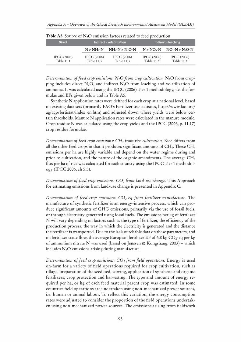
Determination of feed crop emissions: N2O from crop cultivation. N2O from crop-ping includes direct N2O, and indirect N2O from leaching and volatilization of ammonia. It was calculated using the IPCC (2006) Tier 1 methodology, i.e. the for-mulae and EFs given below and in Table A5.

Synthetic N application rates were defined for each crop at a national level, based on existing data sets (primarily FAO’s Fertilizer use statistics, http://www.fao.org/ag/agp/fertistat/index_en.htm) and adjusted down where yields were below cer-tain thresholds. Manure N application rates were calculated in the manure module. Crop residue N was calculated using the crop yields and the IPCC (2006, p. 11.17) crop residue formulae.

Determination of feed crop emissions: CH4 from rice cultivation. Rice differs from all the other feed crops in that it produces significant amounts of CH4. These CH4

emissions per ha are highly variable and depend on the water regime during and prior to cultivation, and the nature of the organic amendments. The average CH4

flux per ha of rice was calculated for each country using the IPCC Tier 1 methodol-ogy (IPCC 2006, ch 5.5).

Determination of feed crop emissions: CO2 from land-use change. This Approach for estimating emissions from land-use change is presented in Appendix C.

Determination of feed crop emissions: CO2-eq from fertilizer manufacture. The manufacture of synthetic fertilizer is an energy-intensive process, which can pro-duce significant amounts of GHG emissions, primarily via the use of fossil fuels, or through electricity generated using fossil fuels. The emissions per kg of fertilizer N will vary depending on factors such as the type of fertilizer, the efficiency of the production process, the way in which the electricity is generated and the distance the fertilizer is transported. Due to the lack of reliable data on these parameters, and on fertilizer trade flow, the average European fertilizer EF of 6.8 kg CO2-eq per kg of ammonium nitrate N was used (based on Jenssen & Kongshaug, 2003) – which includes N2O emissions arising during manufacture.

Determination of feed crop emissions: CO2 from field operations. Energy is used on-farm for a variety of field operations required for crop cultivation, such as tillage, preparation of the seed bed, sowing, application of synthetic and organic fertilizers, crop protection and harvesting. The type and amount of energy re-quired per ha, or kg of each feed material parent crop was estimated. In some countries field operations are undertaken using non-mechanized power sources, i.e. human or animal labour. To reflect this variation, the energy consumption rates were adjusted to consider the proportion of the field operations undertak-en using non-mechanized power sources. The emissions arising from fieldwork

Table A5. Source of N2O emission factors related to feed productiondirect indirect - volatilization indirect - leaching

N > NH3-N NH3-N > N2O-N N > NO3-N NO3-N > N2O-N

IPCC (2006) Table 11.1





94


per ha of each crop were calculated by multiplying the amount of each energy type consumed per ha by the emissions factor for that energy source.

Determination of feed crop emissions: CO2 from transport and processing. Swill and lo-cal feeds, by definition, are transported minimal distances and are allocated zero emis-sions for transport. Non-local feeds are assumed to be transported between 100 km and 700 km by road to their place of processing. In countries where more of the feed is consumed than is produced (i.e. net importers), feeds that are known to be transported globally (e.g. soymeal) also receive emissions that reflect typical sea transport distances.

Emissions from processing arise from the energy consumed in activities such as milling, crushing and heating, which are used to process whole crop materials into specific products. Therefore, this category of emissions applies primarily to feeds in the by-product category.

Determination of feed crop emissions: CO2 from blending and transport of com-pound feed. In addition, energy is used in feed mills for blending non-local feed materials to produce compound feed and to transport it to its point of sale. It was assumed that 186 MJ of electricity and 188 MJ of gas were required to blend 1 000 kg of DM, and that the average transport distance was 200 km.

Determination of the ration GHG emissions arising from the production of non-crop feed materials. Default values were used for fishmeal, lime and synthetic amino acids (see Table B18).

5.4 Allocation of emissions between the crop and its by-productsIn order to calculate the emission intensity of the feed materials, the emissions need to be allocated between the crop and its by-products, i.e. the crop residue or by-products of crop processing. The general expression used is:

GHGkgDM = GHGha/(DMYGcrop*FUEcrop+DMYGco*FUEco)*EFA/MFA*A2

Where:

GHGkgDM = emissions (of CO2, N2O or CH4) per kg of DMGHGha = emissions per haDMYGcrop = gross crop yield (kg DM/ha)DMYGco = gross crop co-product yield (kg DM/ha)FUEcrop = feed use efficiency, i.e. fraction of crop gross yield harvestedFUEco = feed use efficiency, i.e. fraction of crop co-product gross

yield harvestedEFA = economic fraction, crop or co-product value as a fraction

of the total value (of the crop and co-product) MFA = mass fraction, crop or co-product mass as a fraction of the

total mass (of the crop and co-product)A2 = second grade allocation: ratio of the economic value of second

grade crop to the economic value of its first grade equivalentYields of DM and estimated harvest fractions were used to determine the mass

fractions. Where crop residues were not used, they were assumed to have a value

95


of zero i.e. 100 percent of the emissions were allocated to the crop. In order to re-flect the lower value of the second grade crops (i.e. food crops that fail to meet the required standards and are consequently sold as feed) relative to their first grade equivalents, they were allocated a fraction (A2 = 20 percent) of the total emis-sions arising from their production roughly proportionate to their economic value. Clearly, the relative value could potentially vary for different crops and locations depending on supply and demand, or the extent to which there is a market for sec-ond grade crops and the price of alternative feedstuffs. This is an important assump-tion, which will be investigated and refined in the future.

The allocation of feed emissions is summarized in Table A6 and Figure 3. Note that:•emissions from post-processing blending and transport are allocated entire-

ly to feed;•emissions that are not allocated to feed do not cease to exist; rather, they are,

or should be, allocated to other commodities. For example, if we assume that swill has zero economic value, then the emissions from swill production should be allocated to household food. Similarly, the 80 percent of emis-sions not allocated to second grade crops should be allocated to the remain-ing first grade crops. Failure to follow this approach may lead to incorrect policy conclusions. Overestimating the proportion of crops that fail to meet first grade quality will lead to a reduction in total emissions, rather than an increase in the emission intensity of first grade crops that offsets the decrease in the emission intensity of the second grade crops (see Table A6).

Table A6. Summary of the allocation techniques used in the calculation of plant-based feed emissions

Products Source of emissions Allocation technique

Swill Emissions arising from the production of human food

Assumed to have no economic value, so allocated no emissions

All feed crops and their by-products

N2O from manure applicationN2O from synthetic fertilizerCO2 from fertilizer manufactureCO2 from fieldwork

Allocation between the crop and co-product is based on the mass harvested, and the relative economic values (using digestibility as a proxy)

Local second grade crops only

N2O from manure applicationN2O from synthetic fertilizerCO2 from fertilizer manufactureCO2 from fieldwork

Allocation between crop and co-product is the same as for other feed crops (see above) PLUS local waste crops receive 20 percent of the emis-sions allocated to the crop, to reflect their low economic value. The other 80 percent is effectively allocated to the 1st grade crops.

By-products only CO2 from processing CO2 from LUC (for soybean)

Allocated to the processing by-products based on mass and economic value

Non-local feeds only CO2 from transportation and blending

100 percent to feed material

Source: Authors.

96


6. SySTEM MOduLEThe functions of the system module are:

• to calculate the average energy requirement (kJ) of each animal cohort (adult females, adult males etc.) and the feed intake (kg DM) for its needs;

• to calculate the total emissions and land use arising during the production, processing and transport of the feed;

• to calculate the CH4 and emissions arising during the management of the VSx;• to calculate enteric CH4 emissions.

6.1 Calculation of animal energy requirement The systems module calculates the energy requirement of each animal, in kilojoule (kJ), which is then used to determine the feed intake (in kg of DM). The energy requirement and feed intake are calculated using an IPCC (2006) Tier 2-type ap-proach, i.e. the energy required for each of the metabolic functions is calculated separately then summed. See Tables A7 and A8 for examples of the formulae used, where:

BWavg = average weight of sow or fattening pig (kg/pig)ACT = adjustment for activity level (dimensionless)LSIZE = litter size (no. of piglets per litter)BWGpiglet = weight gain of piglet: birth-weaning (kg)LACT = length of birth-weaning period (days)MWGenergy = milk energy derived from fat stored during pregnancy

rather than feed intake during lactation (kJ/day)DWG = daily weight gain (kg/day)FPROT = fraction of protein in the DWG (dimensionless)FFAT = fraction of fat in the DWG (dimensionless)AFkg = average weight of the laying hen (kg/hen)Pkg = average weight of juvenile chickens (kg/juvenile chicken)TEMP = ambient temperature (˚C)GROWF = laying hen growth rate (kg/day)GROWP = juvenile chicken growth rate (kg/day)EGGKG = weight of eggs laid per day (kg/day)

As the IPCC (2006) does not include equations for calculating the energy require-ment of pigs or poultry, equations were derived from NRC (1998) for pigs and Sa-komura (2004) for chickens. The NRC (1998) pig equations were adjusted in light of recent farm data supplied by Bikker (personal communication 2011). In order to perform the calculations, data from the herd module (i.e. the number of animals in each cohort, their average weights and growth rates, fertility rates and yields) were combined with input data on parameters (egg weight, protein/fat fraction, tempera-ture, activity levels).

Energy required for maintenance will vary depending on the activity levels of the animals. The maintenance energy requirement is, therefore, adjusted in situations where it is likely to be significantly higher, e.g. where ruminants are ranging rather than grazing, or for backyard pigs and poultry, which are scavenging for food. The maintenance energy requirement of cattle and buffalo is also adjusted to reflect the amount of energy expended in field operations by animals that are used for draft.

97


Table A7. Formulae for the calculation of the energy requirements of sows and fattening pigs

Metabolic function Equation for sows1 Equation for fattening pigs1

Maintenance (kJ/day)

443.5*BWavg0.75*(1+ACT)a 443.5*BWavg0.75*(1+ACT)

Growth (kJ/day) a 0.23*DWG*1 000*FPROT*54 +0.90*DWG*1 000*FFAT*52.3

Lactation (kJ/day) LSIZE*(BWGpiglet*1 000*20.59/LACT)-(MWGenergy)

NA

Pregnancy (kJ/day) 148.11*LSIZE NA1 Definition of variables one provided in the text.a Sows do not have growth energy per se, but their weight and, therefore, maintenance energy varies, depending on

their status (i.e. whether they are pregnant, lactating or idle) so the maintenance energy for each of these states is calculated separately, then used to calculate the average maintenance energy, based on the lengths of each period.

NA: Not Applicable.Source: NRC (1998).

Table A8. Formulae for the calculation of the energy requirements of laying hens and pullets

Metabolic function Equation for laying hens1 Equation for juvenile chickens1

Maintenance energy (kJ/day)

AFkg0.75*(692.8-9.9*TEMP)*(1+ACT) Pkg0.75*386.63*(1+ACT)

Growth energy (kJ/day) 27.9*GROWF*1 000 21.17*GROWP*1 000

Egg production (kJ/day) 10.03*EGGKG*1 000 NA1 Definition of variables one provided in the text.NA: Not Applicable.Source: Sakomura N.K. (2004).

It is assumed that layers and broilers are kept in housing with a controlled envi-ronment, and the ambient temperature is a constant 20 ˚C. For backyard chickens, the average annual ambient temperature is used.

6.2 Calculating feed intake, total feed emissions and land useThe feed intake per animal in each cohort (in kg DM/animal/day) is calculated by dividing the animal’s energy requirement (in kJ) by the average ME (poultry) or DE (pigs) content of the ration from the feed module, e.g.:

feed intake adult females (kg DM/animal/day) = energy requirement (kJ/animal/day)/feed energy content (kJ/kg DM)

The feed intake per animal in each cohort is multiplied by the number of animals in each cohort to get the total daily feed intake for the flock/herd.

The feed emissions and land use associated with the feed production are then calculated by multiplying the total feed intake for the flock/herd by the emissions or land use per kg of DM taken from the feed module.

The protein content of the ration is checked at this stage by comparing the aver-age lysine requirement across the flock or herd with the average lysine content of the ration. Assumptions about the proportions of each of the feed materials are ad-justed in situations where the protein content appears to be excessively low or high.

98


6.3 Calculation of CH4 emissions arising during manure managementCalculating the CH4 per head from manure using a Tier 2 approach requires (a) estimation of the rate of VSx per animal and (b) estimation of the proportion of the VS that are converted to CH4. The VSx rates are calculated using Equation 10.24 from IPCC (2006).

Once the VS excretion rate is known, the proportion of the VS converted to CH4

during manure management per animal per year can be calculated using Equation 10.23 from IPCC (2006).

The CH4 conversion factor depends on how the manure is managed. In this study, the manure management categories and EFs in IPCC (2006, Table A7) were used. The proportion of manure managed in each system is based on official statis-tics (such as the Annex I countries’ National Inventory Reports to the UNFCCC), other literature sources and expert judgement. Regional average MCFs are given in Tables B19 to B22.

6.4 Calculation of n2O emissions arising during manure management Calculating the N2O per head from manure using a Tier 2 approach requires (a) es-timation of the rate of N excretion per animal, and (b) estimation of the proportion of the excreted N that is converted to N2O. The N excretion rates are calculated using Equation 10.31 from IPCC (2006).

N intake depends on the feed DM intake and the N content per kg of feed. The feed DM intake depends, in turn, on the animal’s energy requirement (which is cal-culated in the system module, and varies depending on mass, growth rate, egg yield, pregnancy weight gain and lactation rate, and level of activity) and the feed energy content (calculated in the feed track). N retention is the amount of N retained in tissue, either as growth, pregnancy LW gain or eggs. The following N contents were used:

Pig LW: 25 g N/kg LWChicken LW: 28 g N/kg LWEggs: 18.5 g N/kg egg

The rate of conversion of excreted N to N2O depends on the extent to which the conditions required for nitrification, denitrification, leaching and volatilization are present during manure management. The IPCC (2006) default EFs for direct N2O (IPCC 2006, Table 10.21) and indirect via volatilization (IPCC 2006, Table 10.22) are used in this study, along with variable N leaching rates, depending on the agro-ecological zone (see Table A9).

6.5 Quantifying enteric CH4 emissions from pigsThe enteric emissions per pig depend on the amount of feed gross energy (GE) consumed and the proportion of the feed converted to CH4 (Ym), and are calculated using IPCC (2006) equation 10.21.

Table A9. N2O emission factors for manure managementdirect indirect - volatilization indirect - leaching

N > NH3-N NH3-N > N2O -N N > NO3-N NO3-N > N2O-N

IPCC (2006) Table 10.21

IPCC (2006) Table 10.23

IPCC (2006) Table 11.3 Leaching rates* IPCC (2006)

Table 11.3

*FAO calculations based on Velthof et al. (2009).

99


The GE consumed is a function of the amount of energy required by the pig (for maintenance, growth, lactation and gestation) and the energy content of the ration. Two values of Ym were used: 1 percent for adult pigs and 0.39 percent for growing pigs, based on Jørgensen et al. (2011, p. 617); see also Jørgensen (2007) and Jia et al. (2011).

7. ALLOCATiOn MOduLEThe functions of the allocation module are:

• to sum up the total emissions for each animal cohort;• to calculate the amount of each commodity (meat and eggs) produced;• to allocate the emissions to each commodity;• to calculate the total emissions and emission intensity of each commodity.

The allocation module sums the output (meat and eggs) and emissions and al-locates emissions as illustrated by Figure 3.

7.1 Calculation of the total emissions for each animal cohortThe system track calculates the total emissions arising from feed production, ma-nure management and enteric fermentation. Post animal farmgate emissions are cal-culated separately and incorporated into the allocation module (see Appendix D).

7.2 Calculation of the amount of each commodity producedLW is converted to CW and to bone-free meat (BFM) by multiplying by the per-centages given in Table B24. These percentages vary by species and system (and in some cases, country). The conversion of BFM and eggs to protein is based on the assumption that BFM is 18 percent protein by weight and eggs are 11.9 percent.

7.3 Allocation to by-products and calculation of emission intensityFor the monogastric species, emissions are allocated between the edible commod-ities, i.e. meat and eggs. In reality, there are usually significant amounts of other commodities produced during processing, such as skin, feathers and offal. However, the values of these can vary markedly between countries, depending on the market conditions which, in turn, depend on factors such as food safety regulations and consumer preferences. Allocating no emissions to these can lead to an over allocation to meat and eggs. The potential effect of this assumption is explored in Appendix D.

Layers and backyard chickens produce both eggs and meat. The emissions were allocated between these two commodities, using the following method:

a. Quantify the total emissions from animals required for egg production (adult female and adult male breeding chickens, replacement juvenile chick-ens, hens laying eggs for human consumption).

b. Quantify the total emissions from animals not required for egg production, i.e. producing meat only (surplus male juvenile chickens).

c. Allocate emissions to meat and eggs, on the basis of the amount of egg and meat protein produced (see Table A10).

Allocation is undertaken using both physical criteria and economic criteria. While it is recognized that ISO14044 guidance recommends the use of physical criteria be-fore economic criteria (where possible), both approaches have their strengths and weaknesses, and can be useful provided the results are not misinterpreted. Physical criteria reflect the metabolic work required for the production of tissue and the

100


quantities of biophysical resources (e.g. energy, mass, protein) that remain, while economic criteria (such as price) reflect the balance of supply and demand for the resource and the likelihood of the resource being used. These can lead to quite dif-ferent results, which need to be used and interpreted accordingly.

rEFErEnCEsIPCC. 2006. 2006 IPCC Guidelines for National Greenhouse Gas Inventories, pre-

pared by the National Greenhouse Gas Inventories Programme, Eggleston H.S., Buendia L., Miwa K., Ngara T. and Tanabe K. (eds). IGES, Japan.

Jenssen, T.K. & Kongshaug, G. 2003. Energy consumption and greenhouse gas emissions in fertiliser production. The International Fertilizer Society, Proceed-ings No. 509. York, UK.

Jia, Z.Y., Caoa, Z., Liaoa, X.D., Wua, Y.B., Liangb, J.B. & Yuc, B. 2011. Methane production of growing and finishing pigs in southern China. In Special issue: Greenhouse gases in animal agriculture – finding a balance between food and emissions. Animal Feed Science and Technology, vols. 166: 430–435.

Jørgensen, H. 2007. Methane emission by growing pigs and adult sows as influ-enced by fermentation. Livestock Science, 109: 216–219.

Jørgensen, H., Theil, P.K. & Knudsen, E.B.K. 2011. Enteric methane emission from pigs. In Planet earth 2011 – global warming challenges and opportunities for policy and practice. Published online by InTech.

NRC. 1998. Nutrient requirements of swine: 10th Revised Edition. National Acad-emy Press, Washington.

Sakomura, N.K. 2004. Modelling Energy Utilization in Broiler Breeders, Laying Hens and Broilers, Brazilian Journal of Poultry Science/Revista Brasileira de Ciência Avícola, 6(1): 1–11.

Velthof, G. L., Oudendag, D., Witzke, H. R., Asman, W. A. H., Klimont, Z. & Oenema, O. 2009. Integrated assessment of N losses from agriculture in EU-27 using MITERRA-EUROPE. Journal of Environmental Quality, 38(2): 402–417.

You, L., Crespo, S., Guo, Z. Koo, J., Ojo, W., Sebastian, K., Tenorio, T.N., Wood, S. & Wood-Sichra, U. 2010. Spatial Production Allocation Model (SPAM) 2000, Version 3. Release 2 (available at http://MapSPAM.info).

Table A10. Example of the allocation of emissions to meat and eggs on a protein basisPart of flock producing eggs and meat Part of flock producing meat only

Total emissions (kg CO2-eq)

50 000 39 000

Total protein (kg) Eggs: 800 Meat: 200 Meat: 500

Emission intensity of eggs

= 50 000*(800/1 000)/800= 50 kg CO2-eq/kg protein

Emission intensity of meat

= (50 000*(200/1 000) + 39 000)/ (200 + 500)= 70 kg CO2-eq/kg protein

Source: Authors.

101

APPENDIx B

data and data sources

1. dATA rESOLuTiOn And diSAGGrEGATiOnData availability, quality and resolution vary according to parameters and the coun-try in question. In OECD countries, where farming tends to be more regulated, there are often comprehensive national or regional data sets, and in some cases subnational data (e.g. for manure management in dairy in the United States of America). Con-versely, in non-OECD countries, data is often unavailable necessitating the use of re-gional default values (e.g. for many backyard pig and chicken herd/flock parameters). Examples of the spatial resolution of some key parameters are given in Table B1.

Basic input data can be defined as primary data such as animal numbers, herd/flock parameters, mineral fertilizer application rates, temperature, etc. and are data taken from other sources such as literature, databases and surveys. Intermediate data are an output of the modelling procedure required in further calculation in GLEAM and may include data on growth rates, animal cohort groups, feed rations, animal energy requirements, etc.

2. LivESTOCk MAPSMaps of the spatial distribution of each animal species and production systems are one of the key inputs into the GLEAM model. The procedure by which these maps are generated for monogastrics is outlined briefly below.

Total pig and chicken numbers at a national level are reported in FAOSTAT. The spatial distributions used in this study were based on maps developed in the context of FAO’s Global Livestock Impact Mapping System (GLIMS) (Franceschini et al., 2009). Regression (based on reported data of the proportions of backyard pigs) was used to estimate the proportion of the pigs in each country in the backyard herd. A simplified version of the procedure described in FAO (2011), was then used to distribute the back-yard pigs among the rural population, taken from the Global Rural Urban Mapping Project (GRUMP) dataset (CIESIN, 2005). Reported data, supplemented by expert opinion, was used to determine the proportions of the remaining non-backyard pigs in intermediate and industrial systems. The pig mapping method is currently being re-vised and the new method and maps will be reported in Robinson et al. (forthcoming).

A similar procedure was undertaken to determine the spatial distribution of chickens. FAOSTAT production of meat and eggs was used to determine the pro-portions of non-backyard chickens in the layer and broiler flocks.

3. HErd/FLOCk PArAMETErS3.1 Fertility parametersData on fertility are usually incorporated in the form of parturition rates (e.g. calv-ing, kidding, lambing rates) and are normally defined as the number of births oc-curring in a specified female population in a year. For monogastrics, litter/clutch size is taken into account. The model utilizes age-specific fertility rates for adult and young replacement females. The proportion of breeding females that fails to conceive is also included.

102


Table B1. Spatial resolution of the main input variablesParameters Cell1 Subnational national regional2 Global

Herd

Animal numbers X

Weights X X

Mortality, fertility and replacement data X X

Manure

N losses rates X

Management system X X

Leaching rates X

Feed

Crop yields X

Harvested area X

Synthetic N fertilizer rate X

N residues X3 X4

Feed ration X5 X

Digestibility and energy content X X

N content X X

Energy use in fieldwork, transport and processing

X

Transport distances X

Land-use change

Soybean (area and trade) X

Pasture (area and deforestation rate) X

Animal productivity

Yield (milk, eggs, and fibers) X X

Dressing percentage X X

Fat and protein content X X

Product farm gate prices6 X X

Post farm

Transport distances of animals or products X

Energy (processing, cooling, packaging) X

Mean annual temperature X

Direct and indirect energy X X

The spatial resolution of the variable varies geographically and depends on the data availability. For each input variable, the spatial resolution of a given area is defined as the finest available.

1 Animal numbers and mean annual temperature: ~ 5 km x 5 km at the equator; crop yields, harvested area and N residues: ~ 10 km x 10 km at the equator.

2 Geographical regions or agro-ecological zones.3 For monogastrics.4 For ruminants.5 Ruminants: rations in the industrialized countries; Monogastrics: rations of swill and concentrates.6 Only for allocation in small ruminants.

103

Appendix B – Data and data sources

3.2 MortalitiesData on mortality is incorporated in the form of death rates. In the modelling pro-cess, age-specific death rates are used: e. g. mortality rate in piglets and mortality rate in other animal categories. The death rate of piglets reflects the percentage of piglets dying before weaning. This may occur by abortion, still birth or death in the first 30 days after birth.

3.3 Growth ratesGrowth rates and slaughter weights are used to calculate age at slaughter, while for chickens the growth rates were calculated based on the weight and age at slaughter.

3.4 replacement ratesThe replacement rate (i.e. the rate at which breeding animals are replaced by young-er adult animals) for female animals is taken from the literature. Literature reviews did not reveal any data on the replacement rate of male animals, so the replacement rate was defined as the reciprocal value of the age at first parturition, on the assump-tion that farmers will prevent in-breeding by applying this rule. For some animals, such as small ruminants, adult males are exchanged by farmers and, therefore, have two or more service periods.

Herd and flock parameters are presented in Tables B2 to B7.

Table B2. Input herd parameters for backyard pigs averaged over regionParameters russian Fed. E. Europe E & sE Asia South Asia LAC ssA

Weight of adult females (kg) 105 105 104 103 127 64

Weight of adult males (kg) 120 120 120 113 140 71

Weight of piglets at birth (kg) 1.00 1.00 0.97 0.80 1.00 1.00

Weight of weaned piglets (kg) 6.0 6.0 6.0 6.2 6.2 6.0

Weight of slaughter animals (kg) 90 90 85 90 88 60

Daily weight gain for fattening animals (kg/day/animal) 0.40 0.40 0.30 0.32 0.35 0.18

Weaning age (days) 50 50 49 50 50 90

Age at first farrowing (years) 1.5 1.5 1.5 1.5 1.5 1.5

Sows replacement rate (percentage) 10 10 10 10 10 10

Fertility (parturition/sow/year) 1.6 1.6 1.5 1.8 1.6 1.6

Death rate piglets (percentage) 17.0 17.0 17.0 17.0 17.0 22.0

Death rate adult animals (percentage) 2.0 2.0 2.0 2.0 2.0 2.0

Death rate fattening animals (percentage) 3.0 3.0 3.0 3.0 3.0 3.0

Source: Literature, surveys and expert knowledge.

104


Table B3. Input herd parameters for intermediate pigs averaged over regionParameters E. Europe E & sE Asia South Asia LAC ssA

Weight of adult females (kg) 225 175 175 230 225

Weight of adult males (kg) 265 195 195 255 250

Weight of piglets at birth (kg) 1.2 1.2 1.2 1.2 1.2

Weight of weaned piglets (kg) 7 7 7 7 8

Weight of slaughter animals (kg) 100 99 100 100 90

Daily weight gain for fattening animals (kg/day/animal) 0.500 0.475 0.475 0.500 0.300

Weaning age (days) 40 40 40 40 42

Age at first farrowing (years) 1.25 1.25 1.25 1.25 1.25

Sows replacement rate (percentage) 15 15 15 15 15

Fertility (parturition/sow/year) 1.8 1.8 1.8 1.8 1.8

Death rate piglets (percentage) 15.0 15.0 15.0 16.0 20.0

Death rate adult animals (percentage) 3.0 3.0 3.0 3.0 3.0

Death rate fattening animals (percentage) 2.0 2.0 2.0 2.0 1.0


Table B4. Input herd parameters for industrial pigs averaged over regionParameters n. America russian Fed. w. Europe E. Europe E & sE Asia LAC

Weight of adult females (kg) 220 225 225 225 175 230

Weight of adult males (kg) 250 265 265 265 195 255

Weight of piglets at birth (kg) 1.2 1.2 1.2 1.2 1.2 1.2

Weight of weaned piglets (kg) 7.0 7.0 7.1 7.0 7.0 7.0

Weight of slaughter animals (kg) 115 116 116 116 114 115

Daily weight gain for fattening animals (kg/day/animal)

0.66 0.66 0.64 0.66 0.67 0.69

Weaning age (days) 30 34 27 34 30 20

Age at first farrowing (years) 1.25 1.25 1.25 1.25 1.00 1.25

Sows replacement rate (percentage) 48 22 43 22 30 30

Fertility (parturition/sow/year) 2.4 2.1 2.3 2.1 2.1 2.2

Death rate piglets (percentage) 15.0 15.0 13.5 15.0 11.7 15.0

Death rate adult animals (percentage) 6.4 3.4 4.9 3.4 5.6 6.4

Death rate fattening animals (percentage) 7.8 4.7 3.9 4.7 5.0 5.6


105


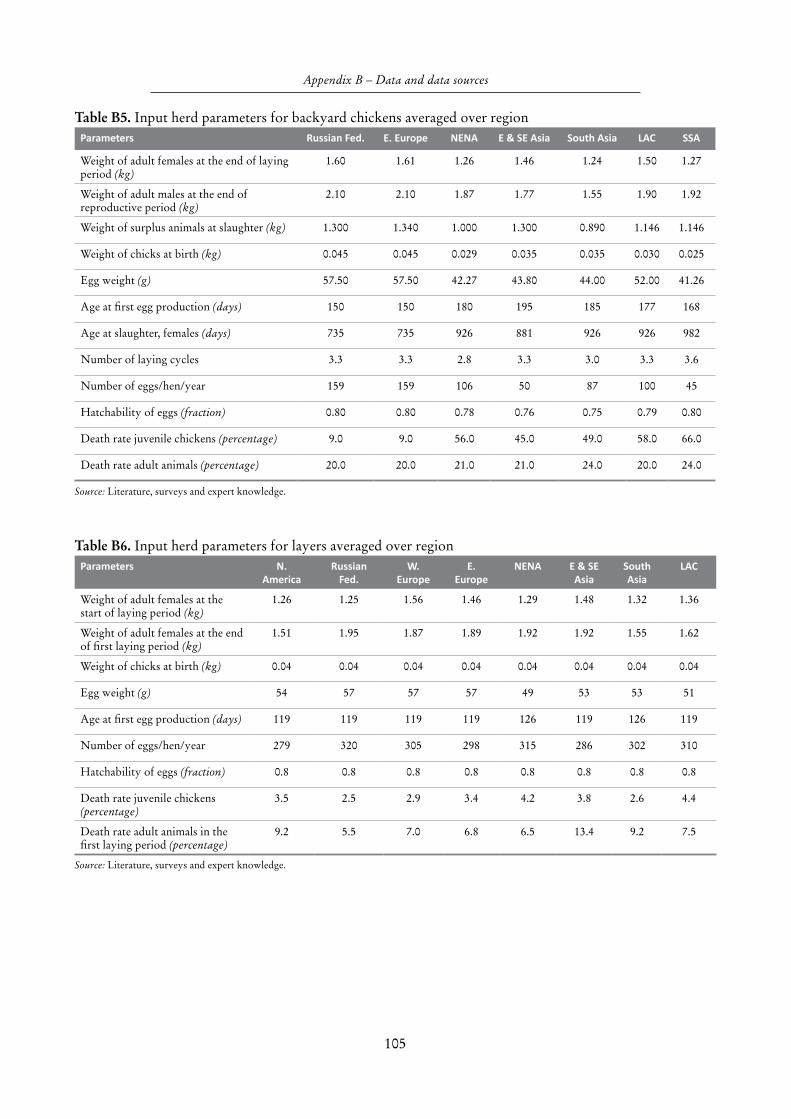
Table B5. Input herd parameters for backyard chickens averaged over regionParameters russian Fed. E. Europe nEnA E & sE Asia South Asia LAC ssA

Weight of adult females at the end of laying period (kg)

1.60 1.61 1.26 1.46 1.24 1.50 1.27

Weight of adult males at the end of reproductive period (kg)

2.10 2.10 1.87 1.77 1.55 1.90 1.92

Weight of surplus animals at slaughter (kg) 1.300 1.340 1.000 1.300 0.890 1.146 1.146

Weight of chicks at birth (kg) 0.045 0.045 0.029 0.035 0.035 0.030 0.025

Egg weight (g) 57.50 57.50 42.27 43.80 44.00 52.00 41.26

Age at first egg production (days) 150 150 180 195 185 177 168

Age at slaughter, females (days) 735 735 926 881 926 926 982

Number of laying cycles 3.3 3.3 2.8 3.3 3.0 3.3 3.6

Number of eggs/hen/year 159 159 106 50 87 100 45

Hatchability of eggs (fraction) 0.80 0.80 0.78 0.76 0.75 0.79 0.80

Death rate juvenile chickens (percentage) 9.0 9.0 56.0 45.0 49.0 58.0 66.0

Death rate adult animals (percentage) 20.0 20.0 21.0 21.0 24.0 20.0 24.0


Table B6. Input herd parameters for layers averaged over regionParameters n.

Americarussian

Fed.w.

EuropeE.

EuropenEnA E & sE

AsiaSouth Asia

LAC

Weight of adult females at the start of laying period (kg)

1.26 1.25 1.56 1.46 1.29 1.48 1.32 1.36

Weight of adult females at the end of first laying period (kg)

1.51 1.95 1.87 1.89 1.92 1.92 1.55 1.62

Weight of chicks at birth (kg) 0.04 0.04 0.04 0.04 0.04 0.04 0.04 0.04

Egg weight (g) 54 57 57 57 49 53 53 51

Age at first egg production (days) 119 119 119 119 126 119 126 119

Number of eggs/hen/year 279 320 305 298 315 286 302 310

Hatchability of eggs (fraction) 0.8 0.8 0.8 0.8 0.8 0.8 0.8 0.8

Death rate juvenile chickens (percentage)

3.5 2.5 2.9 3.4 4.2 3.8 2.6 4.4

Death rate adult animals in the first laying period (percentage)

9.2 5.5 7.0 6.8 6.5 13.4 9.2 7.5


106


4. FEEDThe feed materials used for pigs and chickens are divided into three main categories:

•swill and scavenging•non-local feed materials• locally-produced feed materials

The proportions of the three main feed groups making up the ration were defined for each of the production systems, based on literature and expert knowledge. Default regional values were used for minor producing countries. Tables B8 to B15 summarize the average feed baskets (weighted by total production) for each region and system.

The proportion of the non-local feeds was defined for each country, where pos-sible, using existing literature. For pigs, literature consulted included: FAO (2001); Ndindana et al. (2002); Tra (2003); van der Werf et al. (2005); Grant Clark et al. (2005); FAO (2006); Hu (2007) and Rabobank (2008). For chickens, literature con-sulted included: FAO (2003); Petri and Lemme (2007); Thiele and Pottgüter (2008); Pelletier (2008); FAO (2010); Wiedemann and McGahan (2011); Nielsen et al. (2011); CEREOPA (2011); Jeroch (2011); Leinonen et al. (2012a, 2012b) and Wi-edemann et al. (2012).

Gaps in the literature were filled through discussions with experts (both within FAO and the industry) and also through primary data gathering (a questionnaire survey of commercial egg producers was undertaken with the assistance of the In-ternational Egg Commission). See Tables B8 to B17 for regional averages of ration composition for pigs and chickens per systems and characteristics of feed materials.

In this assessment, all feed materials are identified by three key parameters: dry-matter yield per ha; net energy content (or digestibility) and N content. The DM yield per ha is important because it determines the type of feed ingredients that make up the local feed ration, as well as the potentially available feed (quantity of feed). The digestibility and N content of feed define the nutritional properties of feed. They

Table B7. Input herd parameters for broilers averaged over regionParameters n. America w. Europe E. Europe nEnA E & sE Asia South Asia LAC

Weight of adult females at the start of laying period (kg)

1.25 1.56 1.52 1.31 1.48 1.29 1.34

Weight of adult females at the end of laying period (kg)

1.51 1.88 1.86 1.91 1.89 1.60 1.80

Weight of slaughter broilers (kg) 2.67 2.32 2.19 1.92 2.07 2.00 2.47

Weight of chicks at birth (kg) 0.04 0.04 0.04 0.04 0.04 0.04 0.04

Egg weight (g) 54 57 57 48 50 50 51

Age at first reproduction (days) 119 119 119 119 133 119 119

Age at slaughter, broilers (days) 44 44 40 40 44 40 44

Number of eggs/hen/year 278 305 291 305 289 273 313

Hatchability of eggs (fraction) 0.80 0.80 0.80 0.80 0.80 0.79 0.80

Death rate juvenile chickens (percentage)

3.46 2.80 3.80 4.10 3.70 2.30 4.00

Death rate reproductive animals (percentage)

9.2 6.7 7.3 7.3 12.9 10.4 8.4

Death rate broilers (percentage) 3.6 4.3 4.8 5.9 4.9 5.0 3.0


107


also determine the efficiency with which feed is digested and influences the rate at which GHG emissions are produced. The feed module, additionally, brings together information related to the production of feed, such as fertilization rates, manure ap-plication and energy coefficients for feed production, processing and transport.

The nutritional values of the individual feed materials used to calculate the ration digestibility and N content are given in Tables B16 to B17. These are based on the values in the Dutch Feed Board Feed Database, adjusted from “as fed” to DM basis and aug-mented with data from other sources, such as FEEDIPEDIA (http://www.trc.zootech-nie.fr/node/527) and also the NRC guidelines for pigs and poultry (NRC 1994, 1998).

Table B8. Regional average ration composition by feed category: pigs industrial (percentage) intermediate (percentage) Backyard (percentage)

non-local local SS non-local local SS non-local local SS

LAC 100 0 0 49 50 1 10 70 20

E & SE Asia 100 0 0 49 46 4 10 70 20

E. Europe 100 0 0 69 30 1 17 64 19

N. America 100 0 0 NA NA NA NA NA NA

Oceania 100 0 0 NA NA NA 10 70 20

Russian Fed. 100 0 0 70 30 0 20 60 20

South Asia 100 0 0 50 50 0 10 70 20

SSA 75 25 0 47 50 3 4 78 18

NENA 100 0 0 50 50 0 5 75 20

W. Europe 100 0 0 69 30 0 20 69 10

Global average 100 0 0 52 45 3 10 70 20

NA: Not Applicable – areas with no pig populations.SS: Swill/Scavenging.Source: Literature, surveys and expert knowledge.

Table B9. Regional average ration composition by feed category: chickensindustrial layers (percentage) industrial broilers (percentage) Backyard (percentage)

non-local non-local local SS

LAC 100 100 60a 40a

E & SE Asia 100 100 60b 40b

E. Europe 100 100 80 20

N. America 100 100 80 20

Oceania 100 100 60c 40c

Russian Fed. 100 100 80 20

South Asia 100 100 60 40

SSA 100 100 60 40

NENA 100 100 60d 40d

W. Europe 100 100 80 20a Chile and Mexico have 80 percent local feed and 20 percent swill.b Japan has 80 percent local feed and 20 percent swill.c Australia and New Zealand have 80 percent local feed and 20 percent swill.d Turkey has 80 percent local feed and 20 percent swill.SS: Swill/Scavenging.Source: Literature, surveys and expert knowledge.


108

Table B10. Regional average ration composition and nutritional value: backyard pigsLoCAL feeds* LAC E & sE Asia E. Europe russian Fed. South Asia ssA nEnA Global average

Percentage of feed material in the ration (by mass on a dry matter basis)

GRASSF 0 0 0 0 0 0 1 0

SWILL 19 20 19 20 20 19 20 20

PULSES 0 0 1 1 1 2 0 0

PSTRAW 1 2 7 5 10 14 2 3

CASSAVA 1 0 0 0 0 7 0 0

WHEAT 1 6 12 18 6 0 21 5

MAIZE 5 7 7 1 1 8 5 7

BARLEY 0 0 5 7 0 0 7 1

MILLET 0 0 0 0 1 2 0 0

RICE 2 17 0 0 9 3 0 13

SORGHUM 1 0 0 0 1 3 0 0

SOY 2 1 0 0 0 0 0 1

TOPS 27 5 1 0 16 6 0 7

LEAVES 0 0 0 0 0 0 1 0

BNFRUIT 1 0 0 0 0 2 0 0

BNSTEM 4 0 0 0 2 8 1 1

MLSOY 15 8 1 1 3 1 0 8

MLOILSDS 5 8 17 13 10 9 7 8

MLCTTN 1 1 0 0 2 3 7 1

GRNBYDRY 5 15 12 13 9 8 17 13

nOn-LOCAL feeds* LAC E & sE Asia E. Europe russian Fed. South Asia ssA nEnA Global average


CMLOILSDS 5 5 8 10 5 2 5 5

CMLCTTN 5 5 8 10 5 2 5 5

nutritional values LAC E & sE Asia E. Europe russian Fed. South Asia ssA nEnA Global average

GE (kJ/kg DM) 18 886 18 747 18 835 18 814 18 657 18 501 18 740 18 753

DE (kJ/kg DM) 12 143 12 739 12 512 12 481 11 666 11 852 12 552 12 585

N (g/kg DM) 35.2 34.7 37.5 38.1 30.9 26.7 34.2 34.6

DE/GE (percentage) 64 68 66 66 63 64 67 67

* Definitions of each of the feed names are given in Tables A1 and A2.Source: GLEAM based on input data from literature, national inventory reports, expert knowledge and databases (SPAM, FAOSTAT).

109


Table B11. Regional average ration composition and nutritional value: intermediate pigsLoCAL feeds* LAC E & sE Asia E. Europe russian Fed. South Asia ssA nEnA w. Europe Global average


GRASSF 0 0 0 0 0 0 1 0 0

SWILL 1 4 0 0 0 3 0 0 3

PULSES 0 0 0 0 1 1 0 0 0

PSTRAW 1 1 2 2 7 9 1 2 1

CASSAVA 0 0 0 0 0 7 0 0 0

WHEAT 1 3 9 9 3 0 15 11 3

MAIZE 5 4 2 0 2 4 3 10 4

BARLEY 0 0 3 4 0 0 5 6 1

MILLET 0 0 0 0 1 1 0 0 0

RICE 1 12 0 0 8 2 0 0 9

SORGHUM 1 0 0 0 0 2 0 0 0

SOY 1 1 0 0 0 0 0 0 1

TOPS 18 4 0 0 10 2 0 0 5

LEAVES 0 0 0 0 0 0 1 0 0

BNFRUIT 1 0 0 0 1 1 0 0 0

BNSTEM 3 0 0 0 2 4 1 0 1

MLSOY 9 4 0 1 1 1 0 2 4

MLOILSDS 4 6 7 6 6 8 5 5 6

MLCTTN 1 1 0 0 1 2 5 0 1

GRNBYDRY 4 10 7 7 7 5 12 13 9

nOn-LOCAL feeds* LAC E & sE Asia E. Europe russian Fed. South Asia ssA nEnA w. Europe Global average


CPULSES 0 0 0 0 0 0 0 2 0

CCASSAVA 1 1 0 0 1 7 7 0 1

CWHEAT 8 2 21 24 0 0 0 8 5

CMAIZE 18 25 17 14 6 12 12 12 23

CBARLEY 0 2 6 7 0 0 0 7 2

CMILLET 0 0 0 0 0 7 0 0 0

CRICE 1 3 0 0 12 3 10 0 2

CSORGHUM 4 0 0 0 11 10 0 0 1

CSOY 3 2 0 0 0 0 2 0 2

CMLSOY 10 8 10 10 10 3 12 10 9

CMLOILSDS 0 0 7 7 0 0 0 5 1

CMLCTTN 0 0 0 0 4 0 0 0 0

FISHMEAL 1 1 2 3 2 2 2 0 1

MOLASSES 0 0 0 0 0 1 0 2 0

CGRNBYDRY 1 4 4 4 2 0 2 3 4

SYNTHETIC 1 1 1 1 1 1 1 1 1

nutritional values LAC E & sE Asia E. Europe russian Fed. South Asia ssA nEnA w. Europe Global average

DE (kJ/kg DM) 14 309 14 310 14 616 14 587 13 325 13 710 14 200 14 384 14 310

N (g/kg DM) 33.5 31.8 35.8 36.2 31.4 25.7 34.6 32.5 32.3

DE (percentage) 75 76 77 77 71 74 76 76 76

* Definitions of each of the feed names are given in Tables A1 and A2.Sources: GLEAM based on input data from literature, national inventory reports, expert knowledge and databases (SPAM, FAOSTAT).

110


Table B12a. Regional average ration composition and nutritional value (excluding sub-Saharan Africa): industrial pigs

nOn-LOCAL feeds*

LAC E & sE Asia

E. Europe n. America oceania russian Fed.

South Asia

nEnA w. Europe Global average


CPULSES 0 0 0 0 0 0 0 0 3 1

CCASSAVA 1 1 0 0 0 0 2 15 0 0

CWHEAT 12 4 27 10 20 34 0 0 26 15

CMAIZE 50 55 28 54 0 20 12 24 13 37

CBARLEY 0 3 9 17 16 10 0 0 22 12

CMILLET 0 0 0 0 0 0 0 0 0 0

CRICE 1 3 0 0 0 0 23 20 0 1

CSORGHUM 11 1 0 0 43 0 22 0 0 1

CSOY 2 4 0 0 0 0 1 4 0 1

CMLSOY 19 17 15 11 19 15 21 25 16 15

CMLOILSDS 0 0 10 1 0 10 0 0 11 5

CMLCTTN 0 0 0 0 0 0 9 0 0 0

FISHMEAL 1 1 3 1 0 4 4 5 0 1

MOLASSES 1 0 0 0 0 0 0 0 2 1

CGRNBYDRY 1 9 6 4 0 5 5 5 5 6

SYNTHETIC 2 2 2 2 2 2 2 2 2 2

nutritional values

LAC E & sE Asia


South Asia

nEnA w. Europe Global average

DE (kJ/kg DM) 16 263 15 822 15 227 15 723 15 531 15 188 14 817 15 269 14 762 15 421

N (g/kg DM) 32.5 32.6 37.0 27.6 32.1 38.4 39.5 38.8 36.5 33.3

DE (percentage) 85 83 80 83 82 80 79 81 78 81

* Definitions of each of the feed names are given in Table A1. Sources: GLEAM based on input data from literature, national inventory reports, expert knowledge and databases (SPAM, FAOSTAT).

111


Table B12b. Regional average ration composition and nutritional value in Sub-Saharan Africa: industrial pigs

SSA average ration LoCAL feed (percentage) nOn-LOCAL feed (percentage)

PULSE STRAW 4 NA

CASSAVA 4 11

MAIZE 2 18

MILLET 1 10

RICE 1 5

SORGHUM 1 19

SUGARCANE TOPS 1 NA

BANANA STEM 1 NA

SOYMEAL 1 6

OIL SEED MEAL 5 0

COTTON SEED MEAL 1 0

GRNBYDRY* 3 0

FISH MEAL NA 3

MOLASSES NA 1

SYNTHETIC NA 2

nutritional values SSA average ration

DE (kJ/kg DM) 14 692

N (g/kg DM) 26.4

DE (percentage) 79

* Grain by-products.NA: Not Applicable.Sources: GLEAM based on input data from literature, national inventory reports, expert knowledge and databases (SPAM, FAOSTAT).

112


Table B13. Regional average ration composition and nutritional value: backyard chickens LoCAL Feeds* LAC E & sE Asia E. Europe russian Fed. South Asia ssA nEnA w. Europe Global average


SWILL 40 40 20 20 40 40 40 20 39

PULSES 0 0 1 1 1 2 1 0 0

CASSAVA 2 1 0 0 0 8 0 0 1

WHEAT 1 3 16 27 12 1 15 17 6

MAIZE 7 5 11 1 2 11 2 23 5

BARLEY 0 0 6 10 2 0 4 4 1

MILLET 0 0 0 1 0 3 0 0 0

RICE 6 14 0 0 14 3 1 0 10

SORGHUM 1 0 0 0 0 3 3 0 1

SOY 3 1 0 0 0 0 0 1 1

MLSOY 20 5 1 2 2 2 0 4 6

MLOILSDS 12 18 26 19 6 11 18 8 16

MLCTTN 2 1 0 0 5 6 3 0 2

GRNBYDRY 7 11 17 19 15 11 13 22 12

nutritional values LAC E & sE Asia E. Europe russian Fed. South Asia ssA nEnA w. Europe Global average

ME (kJ/kg DM) 11 582 11 608 11 565 11 550 11 750 12 023 11 787 12 189 11 668

GE (kJ/kg DM) 18 928 18 681 18 825 18 749 18 574 18 601 18 693 18 824 18 699

ME/GE (percentage) 61 62 61 62 63 65 63 65 62

N (g/kg DM) 43.9 37.0 35.7 33.6 32.7 33.3 35.7 30.0 36.8

* Definitions of each of the feed names are given in Table A2.Sources: GLEAM based on input data from literature, national inventory reports, expert knowledge and databases (SPAM, FAOSTAT).

113


Table B14. Regional average ration composition and nutritional value: broilersnOn-LOCAL Feeds*

LAC E & sE Asia


South Asia

ssA nEnA w. Europe Global Average


CWHEAT 0 13 39 0 33 38 18 6 16 40 10

CMAIZE 70 47 28 62 5 30 38 64 44 24 53

CBARLEY 0 4 0 0 7 0 5 0 4 0 1

CSORGHUM 0 7 0 0 21 0 9 0 7 5 3

CSOY 0 0 25 2 3 25 0 0 0 15 3

CMLSOY 28 25 0 24 16 0 24 28 25 10 23

CMLOILSDS 0 1 6 5 2 5 2 0 2 2 2

FISHMEAL 0 1 0 5 5 0 2 0 2 0 2

SYNTHETIC 1 1 1 1 1 1 1 1 1 1 1

RAPESEED 0 0 0 0 1 0 0 0 0 1 0

MLRAPE 0 0 0 0 4 0 0 0 0 1 0

LIME 1 1 1 1 2 1 1 1 1 1 1

nutritional values

LAC E & sE Asia


South Asia


ME (kJ/kg DM)

13 940 13 689 14 484 13 804 13 278 14 583 13 596 13 860 13 656 14 154 13 845

GE (kJ/kg DM)

18 989 18 892 19 831 19 064 18 771 19 831 18 856 18 967 18 878 19 568 19 060

ME/GE (percentage)

73 72 73 72 71 74 72 73 72 72 73

N (g/kg DM) 33.7 34.8 32.8 39.2 37.3 32.2 35.3 34.0 34.9 33.3 35.7


114


Table B15. Regional average ration composition and nutritional value: layersnOn-LOCAL Feeds*

LAC E & sE Asia


South Asia



CWHEAT 4 3 48 2 32 52 30 7 22 44 14

CMAIZE 29 57 9 65 10 0 27 59 42 22 44

CBARLEY 0 0 16 0 0 30 0 0 0 0 2

CSORGHUM 37 0 0 0 21 0 0 0 0 0 4

CSOY 3 18 2 2 4 0 0 3 15 19 12

CMLSOY 14 3 3 22 2 0 8 14 4 1 7

CMLOILSDS 5 3 5 0 9 8 9 9 2 0 4

FISHMEAL 0 0 2 0 5 2 10 0 0 0 1

CGRNBYDRY 0 5 0 0 0 0 8 0 0 1 3

SYNTHETIC 1 1 1 1 1 1 1 1 1 1 1

RAPESEED 0 1 7 0 8 0 0 0 7 4 1

LIME 7 8 7 8 7 7 6 7 7 8 8

nutritional values LAC E & sE Asia


South Asia


ME (kJ/kg DM) 13 177 13 602 13 168 13 152 13 356 12 637 12 503 13 114 13 868 13 791 13 398

GE (kJ/kg DM) 17 855 18 511 18 161 17 735 18 485 17 258 17 683 17 850 18 940 18 641 18 260

ME/GE (percentage)

74 73 73 74 72 73 71 73 73 74 73

N (g/kg DM) 28.7 28.0 27.2 30.1 31.4 24.6 37.1 30.0 28.5 27.6 28.9


115


Table B16. Characteristics of non-local feed materialsname* GE

(kJ/kg of DM)n content

(g/kg of DM)ME

(kJ/kg of DM)ME

(kJ/kg of DM)DE

(kJ/kg of DM)

All Species All Species Chickens Pigs Pigs

CMLSOY 19 960 76.9 9 758 14 621 16 047

CMLOILSDS 19 240 61.8 9 252 11 967 12 893

CMLCTTN 19 240 61.4 8 246 10 053 10 837

PKEXP 19 240 27.0 NA 11 489 11 874

MOLASSES 15 230 9.4 10 463 12 561 12 638

CGRNBYDRY 18 910 28.1 7 292 10 112 10 423

GRNBYWET 20 050 47.2 NA 9 215 9 721

MLRAPE 19 240 56.1 9 252 NA NA

SOYBEAN OIL 39 800 0.0 39 055 NA NA

CPULSES 18 850 39.6 11 319 14 759 15 443

CWHEAT 18 500 20.0 14 506 15 044 15 357

CMAIZE 18 880 15.1 15 839 16 447 16 684

CBARLEY 18 460 18.7 13 112 13 680 13 942

CMILLET 18 680 19.7 13 533 13 714 13 999

CRICE 17 700 13.8 12 551 13 398 13 576

CSORGHUM 18 800 16.9 15 101 15 702 15 969

CCASSAVA 16 900 4.5 13 148 13 580 13 610

CSOY 23 960 61.5 14 945 18 314 19 703

RAPESEED 28 800 34.3 16 490 NA NA

FISHMEAL 18 840 110.3 15 215 15 215 17 522

SYNTHETIC 18 450 160.0 12 000 12 500 15 763

LIME 0 0.0 0 0 0

NA: Not Applicable.* Definitions of each of the feed names are given in Table A1.Source: based on CVB tables (Dutch feed board database), FEEDIPEDIA and NRC (1994, 1998).

116


Table B17. Characteristics of local feed materialsname* GE (kJ/kg of DM) n content (g/kg of DM) ME (kJ/kg of DM) ME (kJ/kg of DM) DE (kJ/kg of DM)

All Species All Species Chickens Pigs Pigs

MLSOY 19 960 76.9 9 758 14 621 16 047

MLOILSDS 19 240 61.8 9 252 11 967 12 893

MLCTTN 19 240 61.4 8 246 10 053 10 837

GRNBYDRY 18 910 28.1 7 292 10 696 11 024

PSTRAW 18 450 8.9 NA 8 889 8 956

TOPS 18 450 9.0 NA 9 500 9 584

BNSTEM 17 900 12.0 NA 9 000 9 116

GRASSF 17 800 27.8 NA 10 556 10 880

LEAVES 19 000 50.0 NA 8 500 9 068

SOY 23 960 61.5 14 945 18 314 19 703

PULSES 18 850 39.6 11 319 14 759 15 443

CASSAVA 16 900 4.5 13 148 13 580 13 610

WHEAT 18 500 20.0 14 506 15 044 15 356

MAIZE 18 880 15.1 15 839 16 447 16 684

BARLEY 18 460 18.7 13 112 13 680 13 942

MILLET 18 680 19.7 13 533 13 714 13 999

RICE 17 700 13.8 12 551 13 398 13 576

SORGHUM 18 800 16.9 15 101 15 702 15 969

BNFRUIT 17 200 8.5 NA 16 092 16 224

SWILL 18 450 35.0 13 000 10 500 10 971

NA: Not Applicable.* Definitions of each of the feed names are given in Table A2.Source: based on CVB tables (Dutch feed board database), FEEDIPEDIA and NRC (1994, 1998).

117


5. EMiSSiOn FACTOrS FOr kEy inPuTS inTO FEEd PrOduCTiOn Emissions of fossil CO2 from feed production, transport and processing are de-pendent on the amount and type of fuel used. Table B18 presents EF used in the calculation of the feed emission intensity.

6. MAnurE MAnAGEMEnTThere are considerable differences in emission between manure management systems (MMSs). Data requirements for the estimation of GHG emissions from MMSs include: information on how manure is managed, the types of MMS, and the proportion of manure managed in these systems. Additionally, climatic infor-mation (e.g. temperature) is important as emission factors are climate dependent. It was, thus, necessary to consider the climate under which livestock is managed in each country.

On a global scale, there are very limited data available on how manure is man-aged and the proportion of the manure managed in each system. Consequently, this study relied on various data sources such as national inventory reports, litera-ture, expert knowledge to define the MMS and the proportions of manure man-aged in these systems. This study uses the IPCC (2006) classification of MMSs (definition in Table 10.18). Regional variations of MMS are presented in Tables B19 to B22.

Quantifying enteric emissions from pigs. The national average Ym in this study var-ies depending on the herd structure, between 0.42 percent and 0.48 percent. This value is lower than the default value used by most Annex I countries using the Tier 2 approach (EEA 2007, Table 6.22), which is based on the IPCC (1997 p4.35 Table A6) values of 0.6 percent for developed countries and 1.3 percent for developing countries (see Table B23).

Table B18. Emission factors used in crop production, non-crop feeds and fuel consumption

EF Source

Ammonium nitrate 6.8 kg CO2-eq/kg N Jenssen and Kongshaug (2003)

Feed

Fishmeal 1.4 kg CO2-eq/kg DM Berglund et al. (2009)

Synthetic 3.6 kg CO2-eq/kg DM Berglund et al. (2009)

Lime 0.079 kg CO2-eq/kg DM FEEDPRINT*

Fuel

Diesel 3.2 kg CO2-eq/l diesel Berglund et al. (2009)

Oil 5.7 kg CO2-eq/kg oil de Boer (2009)

Coal 17.8 kg CO2-eq/kg coal de Boer (2009)

Gas 7.6 kg CO2-eq/m3 gas de Boer (2009)

*http://webapplicaties.wur.nl/software/feedprint/

118

Greenhouse gas emissions from pig and chicken supply chainsTa

ble

B19

. Reg

iona

l ave

rage

man

ure

man

agem

ent a

nd C

H4 a

nd N

2O e

mis

sion

s fa

ctor

s fo

r in

dust

rial

and

inte

rmed

iate

pig

sre

gion

al w

eigh

ted

aver

age

perc

enta

ge o

f man

ure

man

aged

in e

ach

syst

emw

eigh

ted

aver

age

conv

ersi

on fa

ctor

s

Unc

over

ed

anae

robi

c la

goon

Liq

uid/

sl

urry

-

no c

rust

Liq

uid/

sl

urry

-

crus

t

Solid

st

orag

eD

rylo

tPa

stur

e,

rang

e,

padd

ock

Dai

ly

spre

adB

urne

d fo

r fu

elPi

t <

1 m

onth

(P

it1)

Pit

> 1

mon

th

(Pit

2)

Lit

ter

Ana

erob

ic

dige

ster

Met

hane

co

nver

sion

fa

ctor

(p

erce

ntag

e)

kg N

2O-N

/ kg

Nx

LA

C13

1515

1441

02

00

00

023

.60.

014

E &

SE

Asi

a32

1010

06

00

034

00

730

.60.

007

E. E

urop

e7

1515

542

00

03

30

010

.30.

009

N. A

mer

ica

2717

174

30

00

033

00

29.8

0.00

6

Oce

ania

930

00

70

00

00

00

68.9

0.00

6

Rus

sian

Fed

.0

1212

760

00

00

00

05.

00.

009

Sout

h A

sia

1211

1114

330

80

30

08

23.9

0.01

2

SSA

04

46

850

00

10

00

7.1

0.02

1

NE

NA

1015

150

530

00

00

07

11.9

0.01

6

W. E

urop

e6

2727

140

01

01

250

016

.80.

007

Glo

bal a

vera

ge21

1616

108

01

016

100

325

.00.

008

Sour

ce: L

iter

atur

e, s

urve

ys a

nd e

xper

t kno

wle

dge.

Tabl

e B

20. R

egio

nal a

vera

ge m

anur

e m

anag

emen

t and

CH

4 and

N2O

em

issi

ons

fact

ors

for

back

yard

pig

sPe

rcen

tage

of m

anur

e m

anag

ed in

eac

h sy

stem

Glo

bal a

vera

ge c

onve

rsio

n fa

ctor

s

Unc

over

ed

anae

robi

c la

goon

Liq

uid/

sl

urry

-

no c

rust

Liq

uid/

sl

urry

-

crus

t

Solid

st

orag

eD

rylo

tPa

stur

e,

rang

e,

padd

ock

Dai

ly

spre

adB

urne

d fo

r fu

elPi

t <

1 m

onth

(P

it1)

Pit

> 1

mon

th

(Pit

2)

Lit

ter

Ana

erob

ic

dige

ster

Met

hane

co

nver

sion

fa

ctor

(p

erce

ntag

e)

kg N

2O-N

/ kg

Nx

Glo

bal

530

015

155

50

155

05

16.4

0.01

0

Sour

ce: L

iter

atur

e, s

urve

ys a

nd e

xper

t kno

wle

dge.

119


Tabl

e B

21. R

egio

nal a

vera

ge m

anur

e m

anag

emen

t and

CH

4 and

N2O

em

issi

ons

fact

ors

for

laye

rsre

gion

al w

eigh

ted

aver

age

perc

enta

ge o

f man

ure

man

aged

in e

ach

syst

emw

eigh

ted

aver

age

conv

ersi

on fa

ctor

s

Unc

over

ed

anae

robi

c la

goon

Liq

uid/

sl

urry

-

no c

rust

Liq

uid/

sl

urry

-

crus

t

Solid

st

orag

eD

rylo

tPa

stur

e,

rang

e,

padd

ock

Dai

ly

spre

adB

urne

d fo

r fu

elPi

t <

1 m

onth

(P

it1)

Pit

> 1

mon

th

(Pit

2)

Lit

ter

Ana

erob

ic

dige

ster

Met

hane

co

nver

sion

fa

ctor

(p

erce

ntag

e)

kg N

2O-N

/ kg

Nx

LA

C0

3333

350

00

00

00

027

.50.

009

E &

SE

Asi

a0

66

01

23

00

830

026

.00.

009

E. E

urop

e0

00

049

00

00

3317

06.

70.

014

N. A

mer

ica

115

1570

00

00

00

00

8.3

0.00

9

Oce

ania

00

00

023

00

077

00

24.4

0.01

2

Rus

sian

Fed

.0

00

00

00

00

100

00

17.7

0.00

8

Sout

h A

sia

00

010

00

00

00

00

04.

10.

010

SSA

00

00

00

00

090

100

54.2

0.00

8

NE

NA

183

318

00

00

055

20

33.9

0.00

8

W. E

urop

e0

00

2118

01

00

4614

09.

80.

011

Glo

bal a

vera

ge1

88

224

11

00

532

021

.30.

009

Sour

ce: L

iter

atur

e, s

urve

ys a

nd e

xper

t kno

wle

dge.

120


Table B22. Regional average manure management and CH4 and N2O emissions factors for broilers and backyard chickens

Percentage of manure managed in each system weighted average conversion factors

Litter Pasture, range,

paddock

Daily spread Methane conversion factor

(percentage)

kg N2O-N/kg Nx

Broilers 100 1.5 0.005

Backyard 50 50 1.0 0.010


Table B23. Comparison of enteric CH4 emission factors in EU15 and Annex I countries with more than 10 million pigs in 2005

nir implied enteric EF (kg CH4/head/year)

FAO LCA enteric CH4

(kg CH4/head/year)

EU-15 1.00 1.03

Canada 1.50 1.02

Russian Federation 1.50 1.02

United States of America 1.50 0.97

Source: GLEAM.

Table B24. Percentages for the conversion of live weight to carcass weight and carcass weight to bone-free meat

species System Cw/Lw (percentage) BFM/Cw (percentage)

Pigs

Backyard 65 65

Intermediate 75 65

Industrial Country-specific values 65

Chickens

Layers 55 75

Broilers Country-specific values 75

Backyard Laying hens: 55, other chickens: same as broilers 75


rEFErEnCEsBerglund, M., Cederberg, C., Clason, C. & och Lars Törner, M.H. 2009. Jord-

brukets klimatpåverkan – underlag för att beräkna växthusgasutsläpp på gård-snivå och nulägesanalyser av exempelgårdar. Delrapport i JoKer-proJeKtet, Hushållningssällskapet Halland.

CEREOPA. 2011. Available at www.feedbase.com, accessed: 18.01.2011.CIESIN. 2005. Global Rural–Urban Mapping Project (GRUMP) Beta Version.

New York, Center for International Earth Science Information Network (CIE-SIN), Columbia University, New York.

FAO. 2001. Los credos locales en los sistemas tradicionales de producción. FAO, Rome.

FAO. 2003. Poultry feed formulation and preparation good practice in poultry pro-duction in South Asia, by Prabakaran, R. FAO Animal Production and Health Paper No. 159. FAO, Rome.

121


FAO. 2006. Livestock’s long shadow – Environmental issues and options, by Stein-feld, H., Gerber, P., Wassenaar, T., Castel, V., Rosales, M. & de Haan, C. Rome, FAO.

FAO. 2010. Review of the poultry meat sector in Kazakhstan: supply chain analysis and development options, by Willis, G. (Unpublished FAO report).

FAO. 2011. Global livestock production systems, by Robinson, T.P., Thornton, P.K., Franceschini, G., Kruska, R.L., Chiozza, F., Notenbaert, A., Cecchi, G., Her-rero, M., Epprecht, M., Fritz, S., You, L., Conchedda, G. & See, L., FAO, Rome.

Franceschini, G., Robinson, T.P., Morteo, K., Dentale, D., Wint, W. & Otte, J. 2009. The Global Livestock Impact Mapping System (GLIMS) as a tool for ani-mal health applications. Veterinaria Italiana, 45: 491–499.

Grant Clark, O., Moehn, S., Edeogu, I., Price, J. & Leonard, J. 2005. Manipula-tion of dietary protein and nonstarch polysaccharide to control swine manure emissions. J. Environ. Qual., 34: 1461–1466.

Hu, D. 2007. Investigation report on pork supply chains in Zizhong County, Si-chuan Province. China Academy of Agricultural Sciences. (Unpublished manu-script).

Jenssen, T.K. & Kongshaug, G. 2003. Energy consumption and greenhouse gas emissions in fertiliser production. The International Fertiliser Society, Proceed-ings No. 509. York, U.K.

Jeroch, H. 2011. Recommendations for energy and nutrients of layers: a critical review, Lohmann Information, 46(2): 61–72.

Leinonen, I., Williams, A.G., Wiseman, J., Guy, J. & Kyriazakis, I. 2012a. Pre-dicting the environmental impacts of chicken systems in the United Kingdom through a life-cycle assessment: broiler production systems. Poultry Sci., 91(1): 8-25.

Leinonen, I., Williams, A.G., Wiseman, J., Guy, J. & Kyriazakis, I. 2012b. Pre-dicting the environmental impacts of chicken systems in the United Kingdom through a life-cycle assessment: egg production systems. Poultry Sci., 91(1): 26–40.

Ndindana, W., Dzama, K., Ndiweni, P.N.B., Maswaure, S.M. & Chimonyo, M. 2002. Digestibility of fibre diets and performance of growing Zimbabwean indigenous Mukota pigs and exotic Large White pigs fed maize based diets with graded levels of maize cobs. Animal Feed Science and Technology, 97: 199–208.

Nielsen, N., Jørgensen, M. & Bahrndorff, S. 2011. Greenhouse gas emission from the Danish broiler production estimated via LCA methodology. AgroTech/Knowledge Centre for Agriculture. Aarhus, Danemark.

NRC. 1994. Nutrient requirements of poultry: 9th revised edition. National Acad-emy Press. Washington.

NRC. 1998. Nutrient requirements of swine: 10th Revised Edition. Washington: National Academy Press.

Pelletier, N. Lammers, O.P., Stender, D. & Pirog, R. 2010. Life cycle assessment of high- and low-profitability commodity and deep-bedded niche swine produc-tion systems in the upper midwestern United States. Agricultural Systems, 103: 599–608.

Petri, A. & Lemme, A. 2007. Trends and latest issues in broiler diet formulation. Lohmann Information, 42 (2): 25–37.

122


Rabobank. 2008. Animal proteins: costs and commodities. Rabobank, Amsterdam.Robinson, T.P. The global pig sector: production estimates by country and produc-

tion system Life cycle assessment of Australian sugarcane products with a focus on cane processing. AGA Working Paper produced in collaboration with ESS and CCAFS (Forthcoming).

Thiele H., and Pottgüter, R. 2008. Management recommendations for laying hens in deep litter, perchery and free range systems. Lohmann Information, 43(1):53–63.

Tra, H.T.H. 2003. Assessing input in pig production with special focus on feed re-sources and feeding management in demand and resource driven production sys-tems in Son La Province, Vietnam, University of Hohenheim. (MA thesis).

van der Werf, H.M.G., Petit, J. & Sanders, J. 2005. The environmental impacts of the production of concentrated feed: the case of pig feed in Bretagne. Agricul-tural System, 83: 153–177.

Wiedemann, S.G. & McGahan, E.J. 2011. Environmental assessment of an egg production supply chain using life cycle assessment. Final project report. A re-port for the Australian Egg Corporation Limited.

Wiedemann, S.G., McGahan, E. & Poad, P. 2012. Using life cycle assessment to quantify the environmental impact of chicken meat production. Publication, No.12/029. Rural Industries Research and Development, Canberra.

greenhouse gas emissions from pig and chicken supply ... · bpex. 2010. 2009 pig cost of production...

Documents