grundrisk landfill - transport of contaminants released
TRANSCRIPT

GrundRisk Landfill Transport of
contaminants released from landfills
– a part of a risk assessment tool
Environmental Project No. 2080
April 2019

2 The Danish Environmental Protection Agency / GrundRisk Landfill - Transport of contaminants released from landfills - a part of a risk assessment tool
Publisher: The Danish Environmental Protection Agency
Editors: Luca Locatelli, DTU Miljø Poul L. Bjerg, DTU Miljø Philip J. Binning, DTU Miljø
ISBN: 978-87-7038-063-8
The Danish Environmental Protection Agency publishes reports and papers about research and development projects within the environmental sector, financed by the Agency. The content of this publication do not necessarily represent the official views of the Danish Environmental Protection Agency. By publishing this report, the Danish Environmental Protection Agency expresses that the content represents an important contribution to the related discourse on Danish environmental policy.
Sources must be acknowledged.
The Danish Environmental Protection Agency / GrundRisk Landfill - Transport of contaminants released from landfills - a part of a risk assessment tool 3
Contents
Forord 5
Introduktion til metodik for risikovurdering ved deponering af affald 7 Baggrund 7 Metodik til risikovurdering ved deponering af affald 7
Summary and Conclusion 10
1. Introduction 13 1.1 Risk assessment models for landfills 13 1.2 Aim of the project 14 1.3 Model requirements, assumptions and limitations 15 1.4 Link to the “Source term model” 16 1.5 Model outputs 16
2. Description of the contaminant transport models 18 2.1 Model assumptions 19 2.2 Model Affald-A. Single unit located above the top of the aquifer 19 2.2.1 Water balance of an aquifer 20 2.2.2 Model Affald-A. 1D analytical solution of the vertical contaminant transport
model to compute the solute concentration and contaminant mass discharge in the vertical direction 22
2.2.3 Model Affald-A. 3D analytical solution of the horizontal contaminant transport model to compute the solute concentration in the aquifer from a constant source 23
2.2.4 Model Affald-A. Coupling between the horizontal and the vertical transport models 24
2.2.5 Model Affald-A. 1D analytical solution of the horizontal contaminant transport model to compute the time-dependent contaminant mass discharge in the aquifer 25
2.2.6 Model Affald-A parameters 26 2.3 Model Affald-B. Single unit below the top of the aquifer 28 2.3.1 Model Affald-B. 3D analytical solution of the horizontal contaminant transport
model to compute the solute concentration in the aquifer from a constant source 28
2.3.2 Model Affald-B. The model to account for the effect of modified hydrodynamics 30
2.3.3 Model Affald-B. 1D analytical solution of the horizontal contaminant transport model to compute the time-dependent contaminant mass discharge in the aquifer 31
2.3.4 Model Affald-B parameters 32 2.4 Model Affald-A and Model Affald-B common features 32 2.4.1 Solution of the contaminant transport models with a time-dependent
contaminant mass discharge 32 2.4.2 Solution with and without recharge over the aquifer downstream the source 33

4 The Danish Environmental Protection Agency / GrundRisk Landfill - Transport of contaminants released from landfills - a part of a risk assessment tool
2.4.3 1D analytical solution (fully mixed) of the horizontal contaminant transport model to compute the concentrations in the aquifer 34
2.4.4 1D vs 3D analytical solution of the horizontal contaminant transport model to compute the concentrations in the aquifer 35
2.4.5 Solution of multiple spatially distributed landfill units 36
3. Model applications 41 3.1 Tandskov landfill. Application of the model ‘Affald-A’ 41 3.1.1 Geology and hydrogeology 42 3.1.2 Description of the source and the data from Source term model 43 3.1.3 Conceptual model and parameters for Affaldscenter Tandskov 44 3.1.4 Model results for Unit 1 (Afdeling 1) of Affaldscenter Tandskov 46 3.1.5 Results for all four units at Affaldscenter Tandskov 48 3.1.6 Conclusion of the model Affald-A application to the landfill of Tandskov 49 3.2 Faaborg Landfill. Application of the model ‘Affald-B’ 50 3.2.1 Geology and hydrogeology 51 3.2.2 Description of the landfill source 54 3.2.3 Conceptual model and parameters 54 3.2.4 Results for Faaborg Landfill. Model Affald-B 56 3.2.5 Conclusion of the model Affald-B application to the landfill of Faaborg 59 3.3 Hørløkke Landfill. Application of the model ‘Affald-A’ 60 3.3.1 Geology and hydrogeology 60 3.3.2 Description of the landfill source 61 3.3.3 Conceptual model and parameters 61 3.3.4 Model results of Hørløkke Landfill. Model Affald-A 62 3.3.5 Conclusion of the model Affald-A application to the landfill of Hørløkke 65
4. Practical considerations 66
5. References 69
Appendix I 71
Appendix II 74

GrundRisk Landfill - Transport of contaminants released from landfills - a part of a risk assessment tool5
Forord
Miljøstyrelsen, Dansk Affaldsforening og DepoNet har i samarbejde udviklet en ”Metodik til stedsspecifik risikovurdering ved deponering af affald”. Arbejdet er gennemført med opbakning fra branchen, og der har været afholdt møder, hvor branchen har bidraget med kommentarer og input til metodikken. Metodik til stedsspecifik risikovurdering ved deponering af affald består af flere moduler og værktøjer, som er opsummeret i nedenstående oversigt.
• Anvendelse af metodik til risikovurdering ved deponering af affald • Eksempler på anvendelse af metodik
• Modul 1: Beskrivelse af kilden og kildestyrken
o Excelbaseret model til estimering af kildestyrken som funktion af tiden o Brugervejledning til kildestyrkemodellen o Dokumentationsrapport for Fase 1: Konceptuelle modeller o Dokumentationsrapport for Fase 2: Opbygning af kildestyrkemodel
• Modul 2: Stoftransport i jord og grundvand o Modelværktøj - GrundRISK Landfill: Analytisk model til estimering af
stoftransport i umættet og mættet zone (brugerflade baseret på Matlab) o Brugervejledning til GrundRISK Landfill o Dokumentationsrapport for udvikling og tilpasning af GrundRISK modellen til
brug for deponeringsanlæg og lossepladser (GrundRISK Landfill) o Retningslinjer for opstilling af numerisk model til stoftransport i jord og grundvand
• Modul 3: Udsivning, opblanding og vurdering i overfladevand o Notat om opblanding af perkolatforurenet grundvand i overfladevande samt
vurdering af påvirkning i såvel grundvand som overfladevand o Dokumentationsrapport for udvikling af model for opblanding af
perkolatforurenet grundvand i vandløb o Modelværktøj - Mixing of landfill leachate plumes in streams (brugerflade
baseret på Matlab) o Brugervejledning til modellen - Mixing of landfill leachate plumes in streams
Der er i projektet endvidere gennemført en vurdering af miljømæssige og økonomiske konsekvenser ved stedsspecifik risikovurdering ved deponering af affald. Modelværktøjer samt dokumentationsrapporter er samlet på Miljøstyrelsens hjemmeside og kan tilgås via Dansk Affaldsforenings og DepoNets hjemmesider. Denne rapport er udarbejdet som en delopgave under Modul 2: Stoftransport i jord og grundvand

6 GrundRisk Landfill - Transport of contaminants released from landfills - a part of a risk assessment tool
Følgende organisationer og personer har deltaget i arbejdet: Styregruppe: Formand for styregruppen: Anne Elizabeth Kamstrup, Camilla Bjerre Søndergaard, Kåre Svarre Jacobsen, Christian Vind, Miljøstyrelsen, Mikkel Clausen, Niels Bukholt, Lisbet Poll, Miljøstyrelsen Jan Reisz, Miljøstyrelsen Virksomhed Charlotte Fischer, Jacob Hartvig Simonsen, Dansk Affaldsforening Martin Søndergaard, Per Wellendorph, AV Miljø Rasmus Olsen, Odense Renovation Morten Therkildsen, Reno Djurs Koordinationsgruppe: Jette Bjerre Hansen (projektkoordinator), DAKOFA Dagmar Schou, Marie Førby, Jens Aabling, Miljøstyrelsen Inge Lise Therkildsen, Miljøstyrelsen Virksomhed Niels Remtoft, Mette Godiksen, Dansk Affaldsforening Konsulenter og udviklere på delmoduler af metodikken: Modul 1: Beskrivelse af kilden og kildestyrken COWI ved Lizzi Andersen og Steen Stentsøe, Danish Waste Solutions ved Ole Hjelmar, Erik Aagaard Hansen og René Møller Rosendal, ECN ved André van Zommern Modul 2: Stoftransport i jord og grundvand DTU Miljø ved Luca Locatelli, Poul L. Bjerg og Philip J Binning Aagaard Consulting ved Erik Aagaard Hansen Modul 3: Udsivning, opblanding og vurdering af påvirkning i overfladevand og grundvand DTU Miljø ved Grégory Guillaume Lemaire og Poul L. Bjerg Rambøll ved Dorte Harrekilde Vurdering af konsekvenser i relation til at overgå til stedsspecifik risikovurdering ved deponering af affald COWI ved Steen Stentsøe, Lars Grue Jensen og Tage Vikjær Bote Anvendelse af metodik til risikovurdering ved deponering af affald COWI ved Tage Bote Kjær, Danish Waste Solutions ved Ole Hjelmar, DAKOFA ved Jette Bjerre Hansen.

GrundRisk Landfill - Transport of contaminants released from landfills - a part of a risk assessment tool7
Introduktion til metodik for risikovurdering ved deponering af affald
Baggrund I Danmark har vi gennem mange år haft fokus på at beskytte miljøet omkring de danske deponeringsanlæg. EU's deponeringsdirektiv, som indeholder en række foranstaltninger i forhold til miljøbeskyttelse, blev i det væsentligste implementeret i 2001 i Danmark, og senest implementerede vi i 2009 EU’s rådsbeslutninger om kriterier og procedurer for modtagelse af affald til deponering. Ved den danske implementering blev Deponeringsdirektivets krav til miljøbeskyttelse tilpasset de danske forhold ud fra nogle generelle betragtninger, herunder principperne om kystnærhed / ikke-kystnærhed, anlægsfaktorer samt anlægsklasser. Især kystnærhedsprincippet har vist sig at give visse udfordringer, og senest i 2020 må der efter de nuværende regler ikke længere modtages blandet affald til deponering på ikke-kystnære enheder. Branchen har derfor ønsket at få mulighed for at kunne gennemføre en konkret og stedsspecifik vurdering af miljøpåvirkningen fra det enkelte deponeringsanlæg, som et kvalificeret alternativ til de generelle krav i lovgivningen. Samtidig har branchen længe manglet et egentligt værktøj til at kunne estimere miljøpåvirkningen fra deponering af affald som funktion af tiden, og som vil kunne danne grundlag for et kvalificeret estimat af længden af efterbehandlingstiden. Dette er nødvendigt for beregning af den krævede sikkerhedsstillelse. En metodik til vurdering af påvirkning af jord og vandmiljø fra deponeringsanlæg vil derfor kunne bidrage til at få kvalificeret svar på de mange spørgsmål, som er helt centrale i forbindelse med etablering, drift og afslutning af deponeringsanlæg. Metodik til risikovurdering ved deponering af affald Dansk Affaldsforening, Miljøstyrelsen og DepoNet er derfor gået sammen om at udvikle en metodik til stedsspecifik risikovurdering ved deponering af affald i forhold til at synliggøre forureningspåvirkningen af det omkringliggende miljø; grundvand, overfladevand samt natur. Metodikken finder anvendelse for:
• Alle deponeringsanlæg i drift (kystnære og ikke kystnære) • Afsluttede deponeringsanlæg i efterbehandling • Udvidelser af bestående deponeringsanlæg • Planlægning af eventuelle nye deponeringsanlæg • Nedlukkede lossepladser • Nedlagte ukontrollerede lossepladser under den offentlige indsats administreret af
regionerne
De forskellige anlægstyper er nærmere beskrevet i Miljøstyrelsen (2018b). Metodikken er baseret på nyeste viden samt de grundlæggende principper, som også er anvendt i forbindelse med fastsættelse af acceptkriterier for modtagelse af affald på deponeringsanlæg (Bekendtgørelse om deponeringsanlæg, BEK 719:2011). Principperne er illustreret i nedenstående figur.

8 GrundRisk Landfill - Transport of contaminants released from landfills - a part of a risk assessment tool
Afhængig af de stedsspecifikke forhold omfatter metodikken flere af følgende elementer; stoffrigivelse fra det deponerede affald i kilden som funktion af tiden, stoftransport gennem en umættet og mættet zone samt stofudsivning til overfladevand, opblanding og vurdering af påvirkningen i receptor. Metodikken er opbygget i moduler, og hvor det har været muligt anvendes en iterativ arbejdsproces, hvor metodikken indledningsvis er simpel, generisk og konservativ. Efter behov er det muligt at anvende stedsspecifikke data i modellen og inkludere mere avancerede vurderinger. Følgende er indeholdt i metodikken: Anvendelse af metodik til risikovurdering ved deponering af affald Sammenfatningen giver en overordnet beskrivelse af tilgangen anvendt i metodikken samt en trinvis beskrivelse af metodikkens anvendelse. Der gives på hvert trin henvisninger til de konkrete værktøjer, der foreslås anvendt. Sammenfatningen indeholder også et overblik over de forhold, som det ikke har været muligt at afklare endeligt i metodikken samt anbefalinger til hvordan metodikken kan forbedres. Modul 1: Beskrivelse af kilden og kildestyrken Der er opbygget en excel-baseret model til estimering af kildestyrken. Modellen kræver stedsspecifikke data for kildens fysiske udformning samt data for stoffrigivelse (perkolatkoncentration) og perkolatdannelse over tid. Såfremt stedsspecifikke data for stoffrigivelse og perkolatdannelse ikke er tilgængelige, er der i modellen indarbejdet en mulighed for at anvende default værdier. Modellens output beskriver stofkoncentration og perkolatmængde fra kilden som funktion af tiden i overgangen mellem kildens bund og det omkringliggende miljø (kildestyrken). Der er udarbejdet en brugervejledning til modellen samt 2 baggrundsrapporter om principper for opstilling af model samt valg og forudsætninger. Modul 2: Stoftransport i jord og grundvand Beskrivelse af stoftransport i jord og grundvand kan foretages vha. en analytisk model eller en numerisk model. Dette modul indeholder dels en analytisk model udviklet og tilpasset til deponeringsanlæg og lossepladser (GrundRISK Landfill), dels retningslinjer for opstilling af en numerisk model. GrundRISK Landfill er baseret på forholdsvis få stedsspecifikke oplysninger og giver et forsimplet men konservativt billede af, hvordan forureningsstoffer transporteres gennem umættet og mættet zone over tid. Modellen kan regne på flere deponeringsenheder og give et samlet billede for påvirkningen i grundvandet nedstrøms. Model-output fra Kildestyrkemodellen er datainput til såvel GrundRISK Landfill som en numerisk model. Der er udarbejdet en brugervejledning til GrundRISK Landfill samt en dokumentationsrapport for udvikling og tilpasning af modellen.
GrundRisk Landfill - Transport of contaminants released from landfills - a part of a risk assessment tool9
Modul 3: Udsivning, opblanding og vurdering i overfladevand Der er udarbejdet et notat, som giver et overblik over, hvilke receptorer der er relevante at inddrage i forbindelse med vurdering af miljøpåvirkningen fra deponeringsanlæg samt i hvilke situationer. Notatet sammenfatter kriterier for fastsættelse af sammenligningspunktet (point of compliance), miljøkrav og –mål samt praksis for udpegning af blandingszoner. Der gives endvidere et overblik over gældende lovgivning for receptorer. Udsivning af perkolatforurenet grundvand til vandløb har været et særligt opmærksomhedspunkt. Der er opstillet en model til belysning af, hvordan stofudsivning og -spredning i vandløbet sker fra en bred front i brinken, og der er givet anbefalinger til, hvordan påvirkningen af vandløbet vurderes. Der er udarbejdet en brugervejledning til modellen samt en dokumentationsrapport for udviklingen. Vurdering af miljømæssige og økonomiske konsekvenser Der er gennemført en vurdering af de miljømæssige og økonomiske konsekvenser for et deponeringsanlæg ved anvendelse af en stedsspecifik tilgang til vurdering af risiko for påvirkning af det omkringliggende miljø fra påvirkninger relateret til frigivelse af perkolat. Vurderingen omfatter konsekvenserne for det enkelte anlæg og på grundlag heraf er de overordnede konsekvenser ved metodikkens anvendelse for deponering af affald i Danmark vurderet.

10 GrundRisk Landfill - Transport of contaminants released from landfills - a part of a risk assessment tool
Summary and Conclusion
The GrundRisk model (Miljøstyrelsen, 2016b) was developed by DTU and the Danish Environmental Protection Agency (EPA) to assess the risk posed by contaminated sites to groundwater. This report presents the adaptation and application of the GrundRisk model for risk assessment of Danish landfills posing a threat to groundwater and surface water. The new risk assessment tool for landfills (GrundRisk Landfill) consists of two models that simulate contaminant transport from a landfill to the underlying aquifer. The models simulate the dissolved contaminant concentrations in the aquifer as a function of time. The model determines downstream groundwater concentrations given an input contaminant load leaching from landfills, as determined by a separate source term (contaminant source) model (Miljøstyrelsen, 2018a,b). This report presents two new contaminant transport models (Affald-A and Affald-B) for risk assessment of landfills in Denmark. The models have been developed as a part of the project “Methodology for site specific risk assessment of landfilling of waste”. This part of the project addresses the solute vertical and horizontal transport of contaminants released from landfills into soil and groundwater. The model is referred to as GrundRisk Landfill and is implemented in MATLAB. The models for landfills developed are based on GrundRisk (Miljøstyrelsen, 2016b) which is a recently developed groundwater risk assessment tool for contaminated sites aiming to improve risk assessments by including the most relevant transport processes. The models are based on time-dependent analytical solutions and can simulate the time-varying contaminant concentration between the contaminant source and a point of compliance downstream in an underlying groundwater aquifer. This part of the project aims to provide first assessments of the solute transport based on typically sparse data. Because the models are risk assessment tools, conservative assumptions are made when treating uncertainty and when selecting model structure. This report presents the vertical and horizontal transport models and the methods used to couple them. The report demonstrates the model capabilities by applying the models to three landfills in Denmark, one controlled landfill with leachate collection and two old landfills without leachate collection and other measures to prevent groundwater contamination. The models presented in GrundRisk Landfill are a further development of the models presented in Miljøstyrelsen (2016b and 2017). The two models presented in this report are called Affald-A and Affald-B. Affald-A (see Figure 1a) simulates both the vertical contaminant transport processes from the bottom of a landfill to the top of the uppermost groundwater table and the horizontal transport processes in the aquifer. Affald-B (see Figure 1b) simulates the horizontal transport processes in the aquifer from a landfill that is partially immersed in the aquifer. Both are transient models and include the transport processes of advection, diffusion, dispersion, degradation and sorption. The models are based on analytical solutions of the advection-dispersion equation. The model inputs are obtained from a Source term model (Miljøstyrelsen, 2018a,b) and further user-specified hydrogeological and contaminant parameters. The Source term model provides a 500-year time-series (a 500-year period was set by the “steering committee”) of leachate and contaminant concentration at the landfill. The models assume that the velocity in the aquifer is constant and horizontal and that the water balance of the aquifer is not affected by the additional water infiltrating over the area of the

GrundRisk Landfill - Transport of contaminants released from landfills - a part of a risk assessment tool11
landfill. These assumptions can result in an overestimation of the simulated maximum concentrations in the aquifer (as discussed in the model applications). The models were applied to three Danish landfills and showed that contaminant transport processes can reduce maximum concentrations in the underlying aquifers, particularly for highly degradable compounds, compounds retarded by sorption to soil and aquifer materials and/or when the source concentrations steeply decrease in time due to depletion in the source. In the latter case dispersion and dilution processes can attenuate the contaminant concentrations in the aquifer. The case study of the landfill in Tandskov shows the examples of chloride and ammonium in order to demonstrate the applicability of the model (Affald-A). Contaminant concentration and mass discharge in the aquifer 100 m downstream the landfill were simulated. Nickel, chrome and copper (compounds with high sorption) and benzene (degradable) were also simulated. The simulation included both vertical and horizontal transport since the landfill is located in the unsaturated zone tens of meters above the uppermost unconfined aquifer. The results showed that the maximum concentrations of ammonium were slightly reduced, whereas the maximum concentrations of chloride were the same as the maximum input concentrations in the landfill. The lack of contaminant attenuation is due to the fact that the landfill is very large, and so the contaminant mass discharge from the landfill is too large to be diluted and dispersed at a distance of only 100 m downstream of the landfill. Nevertheless, the rapid decrease in time of the source concentration allowed for a small reduction of the maximum concentration of ammonium due to retardation and dispersion. Nickel, chrome and copper from the Tandskov landfill would not reach the POC within the 500 year period because of the high retardation factors would delay the breakthrough curve beyond the 500-year simulation time mainly due to the large vertical transport distance from the landfill to the top of the aquifer. Benzene concentrations at the point of compliance were very low (much lower than the groundwater quality criteria) because of the long transport times and consequent degradation in the aquifer. In addition, for landfills with membrane and leachate collection the concentrations of highly degradable compounds are expected to be relatively low because the degradation to some extend will occur during the period with leachate collection and treatment. However, depending on the substance in question the conditions within the landfill may play a role on the extent of degradation. The case study of the landfill in Faaborg shows the examples of chloride and ammonium in order to demonstrate the applicability of the model (Affald-B). The simulations aimed to determine the ammonium and chloride concentrations and contaminant mass discharge in the aquifer 100 m downstream the landfill. The simulation only included horizontal transport since the landfill is partially submerged in the uppermost aquifer. The results showed that the maximum concentrations of ammonium and chloride were the same as the maximum input concentrations. This is due to the fact that the compounds do not degrade and that the very small groundwater velocity (few meters per year) together with the 10 m thick aquifer does not provide enough water to dilute/disperse the large contaminant mass discharge from the landfill. Moreover, the maximum concentration of ammonium in the aquifer 100 m downstream the landfill occurs after 500 years. This is because of the small groundwater velocity and the sorption processes. Nickel from the Faaborg landfill would not reach the POC within the 500 year period because of the high retardation factors and the very low groundwater velocity. Benzene concentrations at the point of compliance were very low (much lower than the groundwater quality criteria) because of the long transport times and degradation in the aquifer. The case study of the landfill in Hørløkke shows the examples of benzene, iron and nickel in order to demonstrate the applicability of the model (Affald-A). For these substances the concentrations and contaminant mass discharge in the aquifer 100 m downstream the landfill

12 GrundRisk Landfill - Transport of contaminants released from landfills - a part of a risk assessment tool
were simulated. The simulation only included horizontal transport since the landfill is located immediately above the top of the uppermost aquifer (it is not partially submerged). The results showed that the maximum concentrations of iron and nickel are reduced 50% and 70% respectively, mainly due to retardation and dispersion. The maximum concentrations of benzene in the aquifer are reduced due to degradation. Significant reduction of maximum benzene concentrations at the point of compliance are achieved if high degradation rates are assumed. Overall, these examples showed that dispersion and dilution processes are likely to produce a somewhat limited reduction of the maximum source concentrations 100 m downstream of landfills due to the combination of both the large areas of landfills and the somewhat limited transport distance downstream landfills. However, sorption can significantly delay the breakthrough at the point of compliance and degradation processes can significantly reduce both concentrations and contaminant mass discharge at the point of compliance. Our application of the models at three landfill sites, indicates that the current data for Danish landfills are scarce and maybe the biggest limitation for more detailed risk assessment in general. The model Affald-A is designed for landfills with a bottom that is located above the top of the aquifer whereas Affald-B for landfills with a bottom that is located below the top of the water table. Nevertheless, there can be cases where it is not obvious which model to be used and in such cases (i.e. the case study of Faaborg) both models could be applied considering two different transport scenarios. Both models assume uniform groundwater velocity whereas in reality it varies in space and time. The mass discharge from the source is assumed to be uniform throughout the source area and its time variation can be simulated, even though it can be highly uncertain.

GrundRisk Landfill - Transport of contaminants released from landfills - a part of a risk assessment tool13
1. Introduction
1.1 Risk assessment models for landfills A new contaminant transport model GrundRisk Landfill has been developed and it includes two separate models (Affald-A and Affald-B) applicable for different conceptual models. GrundRisk Landfill is a further development and adjustment of a recently developed contaminant transport GrundRisk (Miljøstyrelsen, 2016b; Miljøstyrelsen, 2017). GrundRisk is a new tool that aims to achieve a more realistic risk assessment by including the most relevant contaminant transport processes and thereby ensuring a better identification of contaminant sources posing a risk to groundwater. GrundRisk Landfill aims to simulate the time development of the concentrations and contaminant mass discharge resulting from discharge of landfill leachate into aquifers. The mass discharge from a landfill is time dependent and is obtained from the Source term model (Miljøstyrelsen, 2018a,b). The GrundRisk landfill model is expected to be applicable for the following types of landfills:
- Active controlled landfills with extensive leachate management systems (membrane and leachate collection systems). These landfills have an environmental permit and the release of leachate into the environment is not accepted as long it poses a risk for the surroundings.
- Closed controlled landfills with membrane and leachate collection in aftercare. These landfills have an environmental permit.
- Uncontrolled (old) landfills. These old landfills do not have a permit and leachate has (potentially) uncontrolled entered into the surroundings (groundwater, surface water). The old landfills are regulated by the Soil Contamination Act (Jordforureningsloven) and are part of the public management of soil contamination (”den offentlige indsats for jordforurening”)
These applications are very different as the controlled landfills represent a system, where the leaching has not happened yet, so we aim to predict what will happen when leachate is allowed to enter the environment and in the case it poses an unacceptable impact we aim to predict for how long leachate needs to be collected and treated. These are future scenarios. In addition the models should also be used for decision support when granting environmental permits for new landfills in Denmark or new landfill units. For old landfills the leaching has been going on for many years, and a landfill leachate has already been formed. In this case the models can be used to assess current and future risk. Notably, these different situations are also belonging under different legislations, regulatory frameworks and authorities. Landfills are complex systems that have large sizes, complex waste composition, and multiple units and the landfill leachate plume can under transport be affected by biogeochemical processes. Thus the models are based on several conservative assumptions and simplifications that are thought to be reasonable since the models are risk assessment tools to be used in a regulatory context (and not advanced solute transport models). The conceptual models must be simple, computationally fast and the number of input parameters low. The models include advection/dispersion, sorption and degradation while dissolution/precipitation processes, cation exchange and sequential degradation are neglected. GrundRisk Landfill contains two models (Affald-A and Affald-B) covering the two most typical risk assessment situations for landfills. Model Affald-A (Figure 1a) is designed for landfills that

14 GrundRisk Landfill - Transport of contaminants released from landfills - a part of a risk assessment tool
are situated above the groundwater aquifer and therefore couple a vertical and a horizontal transport model. Model Affald-B (Figure 1b) is designed for landfills that mainly are situated below the groundwater table and thus includes a horizontal transport model only. An example of Model Affald-B could be an old landfill in a former gravel pit, where the groundwater table has been allowed to rise after the pit has been filled. The vertical transport model simulates the contaminant concentration between the contaminant source and the top of the uppermost groundwater aquifer as a function of time. The horizontal transport model simulates the concentrations in the aquifer as a function of time. Both models simulate the contaminant concentrations and mass discharge as a function of time in the aquifer based on the input concentration and leachate in the source. The time-series of input concentrations and leachate are calculated using the Source term model (Miljøstyrelsen, 2018a,b). The models can also simulate multiple different units within the same landfill. Each unit has a different input time series of contaminant concentration and water discharge.
Figure 1. Conceptual figures showing the two GrundRisk models that simulate the contaminant transport processes from a landfill to a point of compliance in the aquifer. (a) Affald-A consists of a vertical and a horizontal transport model. (b) Affald-B consists of a horizontal transport model (and does not include the vertical downward movement of the plume due to groundwater recharge).
1.2 Aim of the project This project aims to develop two new contaminant transport models to be used for landfills. The models aim to provide an initial assessment based on generally scarce data. Because it is a risk assessment tool, conservative assumptions are always made when treating uncertainty and when selecting model structure. The idea is to provide realistic results (conservative) without demanding comprehensive (and expensive) site specific investigations. The contaminant transport models include the processes of advection, hydrodynamic dispersion (mechanical dispersion and diffusion), sorption, and degradation. Moreover, the models are time-dependent and can compute multiple spatially distributed units within the same landfill. Overall, the models developed in this report, include the following features in addition to the original GrundRisk model (Miljøstyrelsen, 2016b):
- Model Affald-B as described above - A dynamic solution in order to account for temporal variation in leachate
composition - A solution for multiple sources to account for different landfill units with different
waste composition - A simple model to compute the contaminant mass discharge at the point of
compliance

GrundRisk Landfill - Transport of contaminants released from landfills - a part of a risk assessment tool15
Notably, the development of these new features and the specific issues related to landfills (e.g. large size, complex waste composition, biogeochemical processes and multiple units) and water balances have been a challenge. In particular the water balance in the aquifer and the link to the water balance assumed in the landfill body from the Source term model are a complicating factor for an analytical model tool that assumes constant aquifer properties in time and space. In order to be in line with the GrundRisk models and keep the models simple, the original concepts and assumptions from the GrundRisk models have been preserved as much as possible. Generally, semi-analytical solutions are used in the models because they can provide fast solutions compared to fully 3D numerical solution that can require hours of calculations and specialized softwares. The new models were developed based on the vertical transport models available in the Danish EPA reports of Miljøstyrelsen (2016a), and the GrundRisk steady-state horizontal transport model described in the Danish EPA reports of Miljøstyrelsen (2016b and 2017). In particular, this report aims to:
- Develop a site-specific (“stedsspecifik”) risk assessment for landfills. - Develop the methods needed to apply the vertical and horizontal transport
GrundRisk models to landfills, including the assumptions made and the rationale for the chosen methods.
- Implement the analytical models in the software Matlab. - Demonstrate the new GrundRisk model capabilities by applying the models to
three landfills in Denmark. In particular, the model applications should illustrate the main issues and challenges when modelling contaminant transport from landfills.
Please note, that the outputs of the models only contain the contribution of contaminants from the landfill considered (contribution from other sources with the same kind of contaminant are not included into the model). The two models developed in this report will be delivered with a stand-alone user interface. The user interface was implemented in MATLAB and will be delivered as an executable file which can be used without a MATLAB license. 1.3 Model requirements, assumptions and limitations The two models presented in this report provide transient simulations and include the transport processes of advection, diffusion, dispersion, degradation and sorption. The models are based on analytical solutions of the advection-dispersion equation. The models can simulate multiple different units within the same landfill. Each unit can have a different input time series of contaminant concentration and water discharge. The model inputs are obtained from the Source term model (contaminant source model. Miljøstyrelsen, 2018a,b) and further user-specified hydrogeological and contaminant parameters. The Source term model provides a 500-year time-series (a 500-year period was set by the “steering committee”) of leachate and contaminant concentration at the landfill. The models assume that the velocity in the aquifer is constant and horizontal and that the water balance of the aquifer is not affected by the additional water infiltrating over the area of the landfill. The biggest limitation/challenge in the development of the models has been the assumption that the water balance of the aquifer is not affected by the additional water infiltrating over the landfill area. In fact, it is shown (section 2.2) that the water balance of an aquifer can be affected by the significant amount of water infiltrating from the landfill area. Even though this assumption can be violated the model results are still considered a reliable estimation. In fact,

16 GrundRisk Landfill - Transport of contaminants released from landfills - a part of a risk assessment tool
Appendix II shows that the violation of this assumption in the case study of Tandskov produced a factor of 1.7-2.3 overestimation of the maximum concentrations at the point of compliance which is reasonable for risk assessment model 1.4 Link to the “Source term model” The two models require input time series of the source concentrations and water discharge. These are provided by the Source term model (Miljøstyrelsen, 2018a,b). The Source term model provides the time-series of concentration and water discharge from the landfill area. One time series of concentration and water discharge is needed for each landfill unit. Figure 2 shows an example of the input concentration and water discharge time series (leachate flux) obtained from the Source term model.
Figure 2. Example of model inputs obtained from the Source term model. (a) Concentration as a function of time. (b) Water discharge from the landfill (or landfill unit).
1.5 Model outputs In principle the models can provide results at any location (x,y,z) and time (t). Nevertheless, the outputs provided by the user interface were designed based on the model application needs. The outputs of the user interface are:
- Time-series of contaminant water phase concentrations at a user-specified point of compliance
- Time-series of the contaminant mass discharge at a user-specified point of compliance
- Accumulated mass discharge over the simulation period (500 years) - Maximum concentration in the aquifer and time of occurrence at a user-specified
distance (same distance as distance to point of compliance) downstream of the landfill.
The two new models simulate the time-dependent contaminant water phase concentration when transported vertical from the bottom of the source down to the top of the aquifer and the subsequent horizontal transport in the aquifer downstream of the source. Figure 3 shows examples of the output that can be obtained from the models. Figure 3a shows the simulated average concentrations (as a function of time) over a 2 m long well screen placed 100 m (a different distance could be chosen) downstream of the landfill. The 2 m length of the well screen selected and the 100 m distance to the point of compliance were presented and discussed in Miljøstyrelsen (2016b). Figure 3b shows the simulated contaminant mass discharge (as a function of time) over a (infinite) control plane in the aquifer perpendicular to the groundwater flow and located 100 m downstream of the landfill.
0
500
1000
1500
2000
2500
3000
1973 2073 2173 2273 2373 2473
conc
entr
atio
n [m
g/L]
year
(a) Concentration
0
5000
10000
15000
20000
25000
1973 2073 2173 2273 2373 2473
disc
harg
e [m
3 /y]
year
(b) Water discharge

GrundRisk Landfill - Transport of contaminants released from landfills - a part of a risk assessment tool17
In this report the mathematical solutions and the practical application of the models to three landfills are reported, while the user interface is described in a separate user manual that comes along with the user interface.
Figure 3. Example of model outputs. (a) Concentration (as a function of time) over a 2 m long well screen placed 100 m downstream the landfill. (b) Contaminant mass discharge (as a function of time) over an infinite plane in the aquifer 100 m downstream the landfill. The depth of the center of the plume (where the maximum concentrations occur) downstream the source could be estimated in the GrundRisk model for contaminated sites (Miljøstyrelsen, 2016b). However, in the case of landfills the simple approach used in Miljøstyrelsen (2016b) is shown to be rough (see Appendix II). Overall, the facts that landfills have large areas; that they can be made of several units with different water discharge; and that they can be partially submerged in the aquifer, make the simple approach very rough and its results are not considered to be reasonable. Therefore, the depth of the center of the plume is not provided as a model output.
0.0
0.1
0.2
0.3
0.4
0.5
0.6
1990 2090 2190 2290 2390 2490
conc
entr
atio
n [m
g/L]
year
(a)
0
100
200
300
400
1990 2090 2190 2290 2390 2490
mas
s dis
char
ge [k
g/y]
year
(b)

18 GrundRisk Landfill - Transport of contaminants released from landfills - a part of a risk assessment tool
2. Description of the contaminant transport models
This chapter describes the two different contaminant transport models designed for landfills, Affald-A and Affald-B. Each model simulates the transport from a source (a landfill unit) or multiple sources to a predefined point of compliance in the aquifer. This chapter describes the conceptual models; the vertical and horizontal transport model equations; the coupling between the vertical and horizontal transport models; and the superposition of different solutions when spatially distributed landfill units are to be simulated. The simulated transport processes are those included in GrundRisk (Miljøstyrelsen, 2016b), namely advection, diffusion and dispersion of the contaminant plume; degradation, and sorption. Each model is based on an analytical time-dependent solution of the mathematical transport equation. The horizontal transport simulation contains both a 1D and 3D model (Also GrundRisk (Miljøstyrelsen, 2016b) contains two different solutions for horizontal transport). Both the 1D and 3D model simulate the concentrations at the point of compliance and then the model giving the highest concentrations is the one adopted. The rationale for introducing a 1D model is that the 3D model was designed for an infinite aquifer and therefore in the case of thin aquifers it can underestimate the concentration because the limited groundwater flux and thickness of the aquifer will constrain the contaminant dilution and dispersion. Therefore, the 1D model provides a better estimate when the aquifer is thin and its groundwater discharge is not much larger compared to the water discharge from the landfill. In this chapter, we first explain the model assumptions; secondly the mathematical equations for both the vertical and horizontal transport from a single unit sources and constant-in-time input contaminant mass discharge; and finally, the methods used to simulate both a time-varying input contaminant mass discharge from a unit source and for landfills that are made of several different units with different source inputs. A landfill can consist of several spatially distributed units/compartments with different characteristics such as specific waste composition, construction characteristics and age leading to different contaminant concentrations, leachate fluxes and time periods. There can be a difference between landfill units and simulated units, i.e. several landfill units may constitute a single model unit depending of the possibility of estimating leaching properties and amounts from the existing landfill units (see documentation report no. 2: Source term). The main challenges of the simple models presented in this report are related to the water balance of the aquifer. The model assumptions are: (1) that the groundwater velocity is constant and horizontal, and (2) that the groundwater flow is not affected by the vertical water flux from the landfill. These assumptions are reasonable for contaminated sites (i.e. for the GrundRisk model of Miljøstyrelsen, 2016a) because contaminated sites are relatively small so that the total amount of water infiltrated over the site area is small compared to the aquifer flow. However, for landfills the site area is typically much larger so that water infiltrated over the site can be a significant contributor to the water balance of the underlying aquifer. This can result in an overestimation of the resulting contaminant concentrations in the aquifer because the vertical advection of contaminants below the source and the dilution due to the additional infiltration of water are ignored.

GrundRisk Landfill - Transport of contaminants released from landfills - a part of a risk assessment tool19
Appendix II shows that the violation of the water balance assumption in the application of the model Affald-A to the case study of Tandskov produced a factor of 1.7-2.3 overestimation of the maximum concentrations at the point of compliance. This is considered acceptable for risk assessment. Model Affald-B includes a model that can reproduce the modified flow field in an aquifer that receives horizontal discharge from a landfill at a different velocity compared to the groundwater velocity. The model results are significantly improved and in better accordance with a fully 3D numerical model taking different flow velocities into account (Appendix I). Nevertheless, the additional water coming from the landfill still it is assumed not to modify the horizontal groundwater velocity of the aquifer. This means that if the difference between the user-input groundwater velocity and the horizontal source velocity is very high (order of magnitude) the user needs first to critically judge the conceptual models and then might reconsider groundwater velocity used in the model or alternatively chose a numerical model for contaminant transport. 2.1 Model assumptions Simple analytical models cannot simulate a detailed water balance because of the requirement that the water velocity is constant. The models therefore make simplifying assumptions to describe downstream contaminant transport. The models are based on the following assumptions:
- Homogenous conditions. This means that the soil and aquifer parameters (e.g. hydraulic properties, water content, porosity, bulk density, and dispersivity) and contaminant parameters (e.g. diffusion coefficient, retardation factors, degradation rates) are constant in space and time.
- Advection only occurs in one dimension (the vertical or horizontal flow direction) with a constant velocity.
- Linear, reversible, instantaneous equilibrium sorption processes between the water and solid phases
- Degradation is described by 1st order kinetics and only occurs in the water phase.
- The model only handles dissolved compounds (separate phase transport of contaminants is excluded).
- Dissolution/precipitation of solid phases and ion exchange processes are not included.
These assumptions/limitations (that have different impacts based on the specific conditions in which the models are applied) are thought to be reasonable since the models are risk assessment tools and not advanced solute transport models. In order to ensure that the model can be used in risk assessments where little data is available, the conceptual models must be simple, computationally fast and the number of input parameters low. 2.2 Model Affald-A. Single unit located above the top of the
aquifer The conceptual model of Affald-A for a single unit source is shown in Figure 4. Affald-A simulates the water phase concentrations in the saturated/unsaturated zone from the bottom of a landfill unit to the top of the aquifer using a vertical transport model, and then the concentrations in the underlying aquifer using a horizontal transport model. The bottom of a unit can be located below terrain level and it has a user-specified distance to the top of the aquifer. The contaminant source have time-dependent input concentrations C0(t) and water discharge Q0(t) (obtained from the Source term model, Miljøstyrelsen, 2018a,b).

20 GrundRisk Landfill - Transport of contaminants released from landfills - a part of a risk assessment tool
Figure 4. Conceptual model of Affald-A showing both vertical and horizontal transport. The contaminant source area at the top of the aquifer is the same as the landfill unit area LxLy; the input concentration at the top of the aquifer C1(t) is the output of the vertical transport model and the water discharge Q0(t) at the top of the aquifer.
The vertical transport model of Affald-A simulates the concentrations between the bottom of the landfill unit and the top of the aquifer using a 1D time-dependent analytical solution that assumes that the horizontal mixing (dispersion) is negligible (there is no variation in concentrations in the y and x directions of the vertical transport). The vertical transport model can simulate the contaminant transport under both unsaturated and saturated conditions. However, in the case of unsaturated conditions, it is assumed that gas diffusion is negligible (this is a conservative assumption). The output of the vertical transport model is a time series of concentration C1(t) and water discharge at the top of the aquifer Q0(t) (assumed to be the same as the water discharge from the source). The time-dependent concentration and discharge at the top of the aquifer are then used as input to the horizontal transport model to compute the concentrations and contaminant mass discharge downstream in the aquifer. The horizontal transport model assumes that the added water discharge Q0 is negligible compared to the groundwater flow and so does not influence the groundwater flow velocity in the aquifer. The horizontal model simulates the time-dependent concentrations in the aquifer based on a 3D time-dependent analytical solution that includes advection, dispersion, degradation, and sorption in the aquifer. In the next subsection, we describe the water balance of an aquifer and its effect on the model assumption of uniform and constant horizontal flow velocity in the aquifer. The following sections describe the analytical solutions of the vertical and horizontal transport models that were developed for constant in time contaminant sources; the coupling between the vertical and the horizontal transport models; the model used to compute the contaminant mass discharge and the model parameters. 2.2.1 Water balance of an aquifer This section discusses the aquifer water balance assumptions. The model Affald-A assumes uniform and constant horizontal flow velocities in the aquifer since the amount water infiltrating from the landfill is assumed to be small compared to the groundwater flow. Therefore, the dilution due to the additional water discharge and the horizontal and vertical variation of the groundwater flow velocity are ignored. Figure 5 visualizes these assumptions and their
y
Top of the aquifer
Terrain level
Lx
Ly
x
z
Contaminantplume
Bottom of a landfill’s unit
AquiferGroundwater flow direction
Point of compliance
Lx
Ly
Satu
rate
d/un
satu
rate
dzo
neSa
tura
ted
zone
C1(
t), Q
0(t)
C0(
t), Q
0(t)

GrundRisk Landfill - Transport of contaminants released from landfills - a part of a risk assessment tool21
implications for the water balance of the aquifer. Figure 5 shows the streamlines and horizontal velocity computed using the simple water balance approach of Appelo and Postma (1993) for an example aquifer which is 15 m thick, has a 0.2 m/y recharge and a water divide at the left boundary (simulated by a no flow boundary conditions). The aquifer has a simplified rectangular geometry which is confined at the bottom and at the upstream side, and is unconfined aquifer with uniform recharge at the top. Two hypothetical landfills are added on the top boundary and illustrate how the flow field below a landfill is dependent on the hydrogeological conditions in the aquifer. The figure shows that (1) the groundwater velocity in the aquifer increases with distance from the groundwater divide (the upstream no-flow boundary); (2) that the groundwater velocity below the landfills varies most near the groundwater divide; (3) the streamlines (that also give an idea of the vertical flow direction/advection) change depending on the horizontal velocities. The main implications of these observations for the Affald-A model are:
- There are vertical groundwater flow velocities below the two landfills and these vertical velocities (vertical advection) are not included into the model.
- There is a significant variation in horizontal groundwater velocities below the two landfills due to the additional recharge/leachate in the landfill area with larger relative changes occurring for the most upstream landfill. The models can only assume a constant velocity. We suggest that the user specified velocity to be input in the model Affald-A is the velocity at the most downstream point of the landfill. This is because the downstream velocity somehow accounts for the additional water infiltrating below the landfill (a more upstream velocity might be too conservative). The model does not account for the additional water that is added through the source area. This may underestimate the dilution particularly for large amounts of water discharge and limited distances to the point of compliance (the assumption that the groundwater flow is not affected by the water discharge from the landfill is more acceptable at large distances from the landfill).
Figure 5. Example of groundwater streamlines (top) and horizontal groundwater velocity (bottom) in an aquifer with constant recharge and no flow boundary conditions. The figure also shows 2 hypothetical landfills and the differences in groundwater
0
20
40
60
80
100
120
0 500 1000 1500 2000 2500
horiz
onta
l gro
undw
ater
ve
loci
ty [m
/y]
x distance from the groundwater divide [m]
landfill 1
100% increase
16% increase
landfill 2
-15
-12
-9
-6
-3
0
0 500 1000 1500 2000 2500dept
h be
low
the
top
of th
e aq
uife
r [m
]
landfill 1 landfill 2
Bottom of the aquifer
Recharge = 0.2 m/y
No
flow
bou
ndar
y

22 GrundRisk Landfill - Transport of contaminants released from landfills - a part of a risk assessment tool
streamlines and velocities depending on how far the 2 landfills are located from the groundwater divide (x=0 m). To address the water balance issue, several changes were attempted to the GrundRisk model Affald-A (i.e. addition of a vertical advective component to the horizontal transport model; introduction of a mixing/dilution zone below the landfill; increase of the groundwater velocity to account for the additional water discharge). However, such changes would raise other problems and therefore were not implemented. 2.2.2 Model Affald-A. 1D analytical solution of the vertical
contaminant transport model to compute the solute concentration and contaminant mass discharge in the vertical direction
Model Affald-A has a time-dependent analytical solution for computing the vertical contaminant transport from a single landfill unit to the underlying groundwater aquifer. The input time series of contaminant mass discharge from the source (the input concentration and vertical water flow from the source), is calculated by the Source term model. The soil layer above the aquifer can be saturated or unsaturated. The transport processes included are percolation (advection) of the contaminant with the vertical water flow from the landfill unit; degradation and sorption. The model does not include dispersion. Lateral dispersion (in the x and y directions) has a minor effect in the case of saturated vertical transport (Miljøstyrelsen, 2016a and 2007), also in the case of volatile compounds in unsaturated zones (because of gas diffusion) the effect of lateral dispersion is assumed to be small due to the large source area typical of landfills (Troldborg et al, 2009). The longitudinal dispersion in the vertical direction (z direction) is assumed to have a small impact since the changes in the contaminant mass discharge from the source usually occur over much longer time scales compared to the longitudinal dispersion time scale. Nevertheless, dispersion can have an effect in the cases where both the changes of concentration in time at the source are significant over short time and the vertical transport time is large. The vertical transport model equation of Affald-A is:
( ) *0 ( ) exp( ); if ( )<0 then ( ) 0i i ic t C t t t t t c tλ= − − =
*/i vt Z v= * / Rλ λ= ; * /v v R=
ti transport time from the bottom of the source to the top of the aquifer λ first order degradation rate R retardation factor C0 source water concentration Zv vertical distance from the source v velocity in the z direction
Equation 1
A 1D solution that includes vertical dispersion (z direction) was presented in Miljøstyrelsen (2016a and 2007). However, it was decided here not to include dispersion in the vertical transport component of model Affald-A to keep the model simple (fewer model parameters required) and for computational reasons (less numerical discretization). As will be also discussed in a later section, the vertical model needs to be able to account for variations in the vertical flow velocities (e.g. due to changes from a situation with leachate collection (pumping)
GrundRisk Landfill - Transport of contaminants released from landfills - a part of a risk assessment tool23
to a situation without) and to do this with a 1D solution with vertical dispersion would require numerical discretization in both time and space (in space because the vertical velocity is not constant). The influence on model results will be discussed later in the report under model applications (Chapter 3). 2.2.3 Model Affald-A. 3D analytical solution of the horizontal
contaminant transport model to compute the solute concentration in the aquifer from a constant source
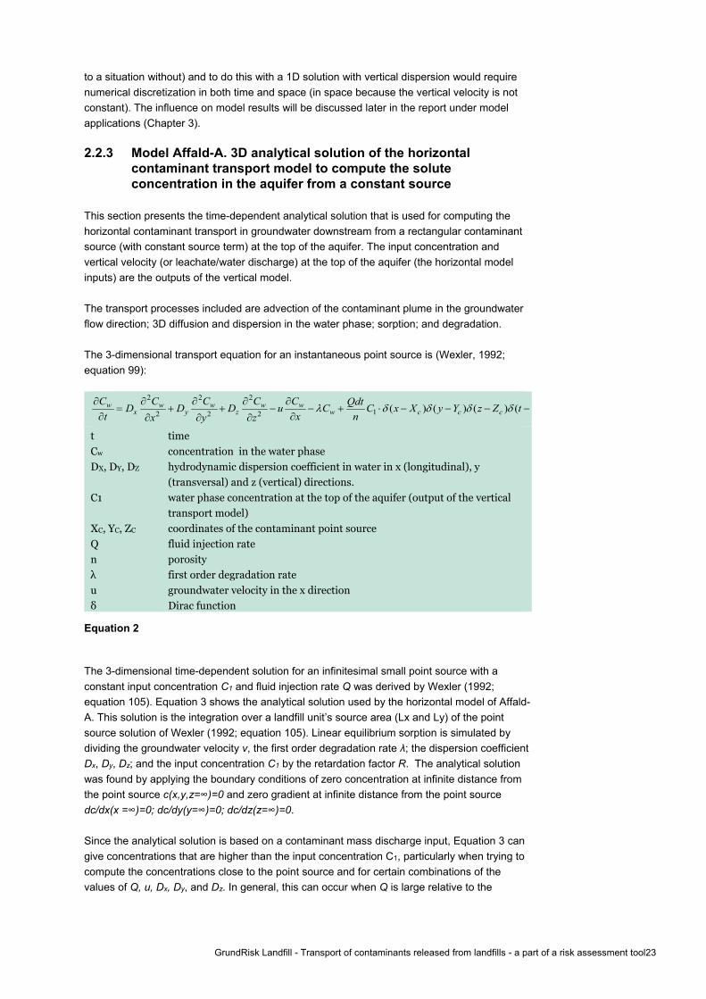
This section presents the time-dependent analytical solution that is used for computing the horizontal contaminant transport in groundwater downstream from a rectangular contaminant source (with constant source term) at the top of the aquifer. The input concentration and vertical velocity (or leachate/water discharge) at the top of the aquifer (the horizontal model inputs) are the outputs of the vertical model. The transport processes included are advection of the contaminant plume in the groundwater flow direction; 3D diffusion and dispersion in the water phase; sorption; and degradation. The 3-dimensional transport equation for an instantaneous point source is (Wexler, 1992; equation 99):
2 2 2
12 2 2 ( ) ( ) ( ) (w w w w wx y z w c c c
C C C C C QdtD D D u C C x X y Y z Z tt x nx y z
λ δ δ δ δ∂ ∂ ∂ ∂ ∂
= + + − − + ⋅ − − − −∂ ∂∂ ∂ ∂
t time Cw concentration in the water phase DX, DY, DZ hydrodynamic dispersion coefficient in water in x (longitudinal), y (transversal) and z (vertical) directions. C1 water phase concentration at the top of the aquifer (output of the vertical transport model) XC, YC, ZC coordinates of the contaminant point source Q fluid injection rate n porosity λ first order degradation rate u groundwater velocity in the x direction δ Dirac function
Equation 2
The 3-dimensional time-dependent solution for an infinitesimal small point source with a constant input concentration C1 and fluid injection rate Q was derived by Wexler (1992; equation 105). Equation 3 shows the analytical solution used by the horizontal model of Affald-A. This solution is the integration over a landfill unit’s source area (Lx and Ly) of the point source solution of Wexler (1992; equation 105). Linear equilibrium sorption is simulated by dividing the groundwater velocity v, the first order degradation rate λ; the dispersion coefficient Dx, Dy, Dz; and the input concentration C1 by the retardation factor R. The analytical solution was found by applying the boundary conditions of zero concentration at infinite distance from the point source c(x,y,z=∞)=0 and zero gradient at infinite distance from the point source dc/dx(x =∞)=0; dc/dy(y=∞)=0; dc/dz(z=∞)=0. Since the analytical solution is based on a contaminant mass discharge input, Equation 3 can give concentrations that are higher than the input concentration C1, particularly when trying to compute the concentrations close to the point source and for certain combinations of the values of Q, u, Dx, Dy, and Dz. In general, this can occur when Q is large relative to the

24 GrundRisk Landfill - Transport of contaminants released from landfills - a part of a risk assessment tool
distance to the simulated point and to the groundwater flux of the aquifer as discussed in previous chapters (the aquifer water balance approximation). If the resulting concentrations are higher than the input concentration then the model reset the concentration to be equal to the maximum input concentration because output concentrations higher than input concentrations are physically unacceptable. This does not affect the mass balance output since the mass balance output is calculated with another model (section 2.2.5). This will be further explored in the model applications in chapter 3.
( )
( )**
/2 1 *
* ** * * *0 /2
exp2
, , , exp exp2 28 2 2
yx
y
cLL
xc
x xL y z x x
u x XC Q
D t tc x y z t erfc erfc dX dD Dn D D D t D t
βγ γ β βγ γ β
π γ−
− + − − = +
∫ ∫
( )1
2*2 * *4 xu Dβ λ= +
( ) ( )* *
2 22 2* *x x
c cy z
D Dx X y Y z
D Dγ = − + − +
x LD uα= ; y TD uα= ; z VD uα=
* /u u R= ; * / Rλ λ= ; *1 1 /C C R=
* /x xD D R= ; * /y yD D R= ; * /z zD D R=
C1 water phase concentration at the top of the aquifer (output of the vertical transport model) Lx length of the source Ly width of the source z depth below the top of the aquifer Q fluid injection rate per unit area n porosity αt, αl, αv transversal, longitudinal and vertical dispersivity in the water phase Dx, Dy, Dz longitudinal (x), transversal (y), and vertical (z) dispersion coefficients λ first order degradation rate u groundwater velocity in the x direction R retardation factor
Equation 3
2.2.4 Model Affald-A. Coupling between the horizontal and the vertical
transport models The conceptual model used for coupling the vertical and the horizontal transport model was shown in Figure 4. The horizontal transport model requires the input area parameters Lx and Ly, the concentration C1(t) and the water discharge Q0(t). The concentration C1 is the output of the vertical transport model at the user specified distance Z between the bottom of the contaminant source and the top of the aquifer; and the water discharge Q0(t) is assumed to be constant in the vertical direction below the source. Because transversal dispersion was ignored in the vertical transport model, the contaminant source area at the top of the aquifer is the same as that of the source (this a reasonable assumption for large source areas such as landfills).

GrundRisk Landfill - Transport of contaminants released from landfills - a part of a risk assessment tool25
2.2.5 Model Affald-A. 1D analytical solution of the horizontal contaminant transport model to compute the time-dependent contaminant mass discharge in the aquifer
This section describes the model used to compute the time-dependent contaminant mass discharge through an infinite y-z plane located at a specified distance (usually the point of compliance) in the aquifer perpendicular to the groundwater flow direction. The mass discharge could be obtained by the integration of the concentration distribution over a y-z plane; however, this is computationally demanding since the concentrations over a y-z plane in the aquifer (downstream the source) needs to be computed at each time step. Instead a simplified model is used. The model includes the processes of advection; degradation; and sorption. Dispersion is not included into the model as its effect on the mass discharge over a y-z plane in the aquifer is minor. Transversal (y direction) and vertical (z direction) dispersions do not matter to the groundwater flow direction because we are integrating the mass discharge over an infinite y-z plane. The longitudinal dispersion (x direction) in the aquifer is assumed to have a small impact since the changes in the contaminant mass discharge from the source usually occur over much longer time scales compared to the longitudinal dispersion time scale. Figure 6 shows the conceptual model used to compute the mass discharge at a y-z control plane. The model discretizes the source in the x direction creating N smaller and equal rectangular sources with contaminant mass discharge Ji(t) and a distance di to the y-z control plane. Therefore each source Ji(t) will have a different travel time to the y-z plane and during this time degradation, and sorption occur. Equation 4 is used to compute the mass discharge as a function of time. This equation exploits the fact that the travel time from a small discretized source to the y-z control plane is the same all over the plane since the plane is perpendicular to the flow. Note that in Equation 4, the contaminant mass discharge J(t) at time t at the control plane is calculated using the mass flux at time t-ti at the source, which is then modified by how much degradation occurred over its transport time to the control plane (exp(-ti*λ)). The approach of discretizing the source rather than model it as a single aggregated unit, showed much better agreement with the breakthrough curves resulting from the 3D transport model (smoother peaks and more realistic fronts and tails). This is due to the fact that the source area is large in the direction of the groundwater flow. The peak mass discharge at the POC resulting from the upstream part of the landfill often do not occur at the same time as the peak resulting from the downstream part of the landfill and therefore the resulting peak will be lower.
( ) *
1
, ( ) exp( ); if ( )<0 then ( ) 0 i N
i i i i ii
J x t J t t t t t J tλ=
=
= − − − =∑
*/i it d u=
1x d= * / Rλ λ= ; * /u u R=
J(x=d1, t) contaminant mass discharge at the y-z plane Ji(t) source contaminant mass discharge from each discretized source area ti travel time from each discretized source area to the y-z plain di distance from each discretized source area to the y-z plain λ first order degradation rate u groundwater velocity in the x direction R retardation factor N total number of discretized source areas

26 GrundRisk Landfill - Transport of contaminants released from landfills - a part of a risk assessment tool
Equation 4
Figure 6. Conceptual model used to compute the contaminant mass discharge at a y-z plane at a d1 distance downstream the landfill. The model discretizes the source in the x direction in N source areas each one having a contaminant mass discharge Ji(t) and a distance to the y-z plane di. 2.2.6 Model Affald-A parameters Table 1 summarizes the model input parameters of Affald-A. The input parameters in the table are divided into three categories: Single source parameters, Vertical model parameters, and Horizontal Model parameters. The Single source parameters are the parameters needed for each of the landfill units, i.e. if there are 4 different units in a landfill there will be 4 concentration time series C0(t), 4 water discharge time series Q0(t), 4 distances Z, etc. The model output is the contaminant concentration over a 2 m screen located at a user specified POC distance from the most downstream point of the landfill site.
Table 1. User specified input parameters of the model Affald-A Input
parameter Description
Single source parameters
C0(t) [M/L3] Concentration time series in the water phase at the source, this is provided by the Source term model
Q0(t) [L3/T] Landfill water discharge time series through the source area, this is provided by The Source term model
Z [L] Distance between the bottom of the landfill unit and the top of the aquifer
Lx [L] Source length, this is provided by Source term model
Ly [L] Source width, this is provided by Source term model
Vertical model
k_v [T-1] First order degradation rate
θ_v [-] Water content (fraction of the total volume)
R_v [-] Retardation factor
Horizontal model
H [L] Thickness of the aquifer
I [L/T] Groundwater recharge
u [L/T] Groundwater velocity
k [T-1] First order degradation rate
n [-] Porosity
αL [L] Longitudinal dispersivity (x direction)
αT [L] Transversal dispersivity (y direction)
αV [L] Vertical dispersivity (z direction)
x
z y
Groundwater flow
J1(t)J2(t)
d1
d2
Source
JN(t)

GrundRisk Landfill - Transport of contaminants released from landfills - a part of a risk assessment tool27
R [-] Retardation factor
POC [L] Distance to the point of compliance

28 GrundRisk Landfill - Transport of contaminants released from landfills - a part of a risk assessment tool
2.3 Model Affald-B. Single unit below the top of the aquifer The conceptual model of Affald-B for a single landfill unit source is shown in Figure 7. Affald-B simulates the water phase concentrations from a source that is located within an aquifer into the same aquifer using a horizontal transport model. The contaminant source has time-dependent input concentrations C0(t) and water discharge Q0(t) obtained from the Source term model (Miljøstyrelsen, 2018a,b). The horizontal model simulates the time-dependent concentrations in the aquifer based on a 3D time-dependent analytical solution that includes advection, dispersion, degradation and sorption in the aquifer. The following sections describe the analytical solutions of the horizontal transport models that were developed for constant in time contaminant sources (the superposition of solutions for constant in time contaminant sources allow the simulation of time-dependent sources); the method used to include the effects of a source that has different horizontal water discharge velocity compared to the model groundwater flow velocity; the model used to compute the mass discharge and the model parameters.
Figure 7. Conceptual model of Affald-B showing the horizontal transport from a submerged source. The contaminant source area LzLy is below the top of the aquifer and at the downstream end of a landfill unit; the input concentration at the source area C0(t) and the water discharge Q0(t) are the outputs of the Source term model. Details about the source and water balance are described in detail in Miljøstyrelsen (2018a,b). 2.3.1 Model Affald-B. 3D analytical solution of the horizontal
contaminant transport model to compute the solute concentration in the aquifer from a constant source
This section presents the time-dependent analytical solution for constant contaminant sources that is used for computing the horizontal transport from a specified vertical plane (a LyLz plane) at the downstream end of the landfill unit to the aquifer. The input concentration and the horizontal water discharge velocity over a LyLz source plane are given by the Source term model. The included transport processes are advection of the contaminant plume in the groundwater flow direction; 3D diffusion and dispersion in the water phase; sorption and degradation. The vertical advection and dilution of the plume downstream the landfill due to groundwater recharge was not included in this model. The vertical advection and dilution of the plume downstream of the landfill due to groundwater recharge combined with the time variation of the source water discharge velocity would make the position of the center of the plume vary in time. Therefore finding the maximum would require computing the concentrations at several locations which is computationally very demanding. On the other hands, if recharge is not
Ly Top of the aquifer
Terrain level
Contaminantplume
Aquifer
Groundwater flow direction
Point of compliance
z
x
Lz
Satu
rate
dzo
ne
C0(t), Q0(t)
y

GrundRisk Landfill - Transport of contaminants released from landfills - a part of a risk assessment tool29
included then the maximum concentrations are always found at the groundwater table and the dilution will be underestimated. The 3-dimensional transport equation for an instantaneous point source is shown in the following equation (Wexler, 1992; equation 115).
2 2 2
2 2 2w w w w w
x y z wC C C C C
D D D u Ct xx y z
λ∂ ∂ ∂ ∂ ∂
= + + − −∂ ∂∂ ∂ ∂
t time λ first order degradation rate Cw concentration in the water phase DX, DY, DZ hydrodynamic dispersion coefficients in water in the x (longitudinal), y (transversal) and z direction (transversal) u groundwater velocity in the x direction
Equation 5 The 3-dimensional time-dependent solution for patch source (in the z-y plane) with a constant input concentration C0 was derived by Wexler (1992; equation 121a). Since there can be a difference between the water discharge velocity (=Q/Ly/Lz) and the groundwater velocity, the source area is modified in order to avoid sudden concentration jumps due to different water discharge and groundwater velocities and also to account for the hydrodynamic effects due to a source in the groundwater that has a different velocity (‘source area’ * ’horizontal water discharge velocity’ = ’modified source area’ * ’horizontal groundwater flow velociy’). Equation 6 shows the analytical solution of Wexler that is used in the horizontal model of Affald-B. Linear equilibrium sorption is simulated by dividing the groundwater velocity v, the first order degradation rate λ; and the dispersion coefficient Dx, Dy, Dz by the retardation factor R. The analytical solution was found by applying the boundary conditions of (1) zero concentration at infinite distance from the point source c(x,y,z=∞)=0; (2) zero gradient at infinite distance from the point source dc/dx(x =∞)=0; dc/dy(y=∞)=0; dc/dz(z=∞)=0; and (3) c=C0 at x=0, Y1<y<Y2 and Z1<z<Z2 (within the y-z source plane).
( )
*
0 * *2 23/2 1 2 1 2
* ** * * * *0
exp2
, , , exp4 48 2 2 2 2
tx
x xx y y z z
u xC xD Y y Y y Z z Z zu xc x y z t erfc erfc erfc erfc d
D DD D D D Dτ λ τ
τπ τ τ τ τ−
− − − − = − + − − −
∫
x LD uα= ; y TD uα= ; z VD uα=
* /u u R= ; * / Rλ λ= ; * /x xD D R= ; * /y yD D R= ; * /z zD D R=
C0 water phase concentration at the top of the aquifer (output of the vertical transport model) y1, y2 y coordinates of the upper and lower limits of the solute source z1, z2 z coordinates of the upper and lower limits of the solute source z depth below the top of the aquifer αt, αl, αv transversal, longitudinal and vertical dispersivity in the water phase Dx, Dy, Dz longitudinal (x), transversal (y), and vertical (z) dispersion coefficients λ first order degradation rate u groundwater velocity in the x direction R retardation factor
Equation 6

30 GrundRisk Landfill - Transport of contaminants released from landfills - a part of a risk assessment tool
2.3.2 Model Affald-B. The model to account for the effect of modified hydrodynamics
This section presents how the Affald-B model includes the effect of the modified groundwater hydrodynamics due to the presence of a source that has a water discharge velocity that is different compared to the groundwater flow velocity. The following simple model was introduced as it showed better results compared to a model that did not account for the modified hydrodynamics; the new model was compared to a numerical (Multiphysics) transport model that included a groundwater flow model (see Appendix I). Figure 8 shows the groundwater flow lines downstream a landfill unit that discharges leachate into the groundwater with different velocities compared to the groundwater. Figure 8a shows the case where the groundwater velocity is smaller compared to the source water discharge/ leachate velocity. In this case the groundwater streamlines downstream the source expands both in the y and z direction. Figure 8b shows the case where the groundwater velocity is larger compared to the source water discharge/ leachate velocity. In this case the groundwater streamlines downstream the source converge both in the y and z direction. The new simple model simply modifies the source area input LzLy estimated in the Source term model. A new source area Lz1Ly1 immediately downstream of the source is computed according to Equation 7. This equation shows that the new area Lz1Ly1 is proportional to the ratio between the horizontal source velocity (from the Source term model) and the groundwater velocity (user defined); if the source velocity is larger than the groundwater velocity then the new area Lz1Ly1 is larger than LzLy and vice versa. Moreover, the ratio between the height and the width of the new rectangular area Lz1Ly1 and the input source area LzLy is constant. The new method was tested for ratios of the horizontal source velocity and the groundwater velocity varying between 1/3 and 3. The groundwater hydrodynamics can become complex in the case the groundwater velocity and the source velocity are very different from each other, and such simple model approach can be biased. It can happen that the difference between the user-input groundwater velocity and the horizontal source velocity are very different. This can be due to several reasons: i.e. a) the case study of Faaborg (see section 3.2) simulated an aquifer (the term aquifer might be misleading for such low permeability subsurface materials) with an extremely low groundwater veolocity; b) the presence of a membrane at the bottom of the landfill can result in very high horizontal discharge velocities. If the difference between the user-input groundwater velocity and the horizontal source velocity is very high (order of magnitude) the user need first to critically judge the conceptual models and then might reconsider the model-input groundwater velocity.
1 1S
y z y zGW
VL L L L
V=
1
1
y y
z z
L LL L
=
Ly, Lz user input source width and depth Ly1, Lz1 modelled source width and depth VS vertical water discharge/ leachate velocity from the source VGW horizontal velocity of the groundwater
Equation 7

GrundRisk Landfill - Transport of contaminants released from landfills - a part of a risk assessment tool31
Figure 8. Conceptual figure showing the local change of groundwater streamlines (blue arrows) due to the presence of a source that discharges a leachate with a different velocity (orange arrows) compared to the groundwater velocity. The figure shows changes in flow field in both the horizontal (plan view) and vertical (side view) direction for groundwater velocities larger (a) and smaller (b) than the velocity in the source area. 2.3.3 Model Affald-B. 1D analytical solution of the horizontal
contaminant transport model to compute the time-dependent contaminant mass discharge in the aquifer
This section describes the model used to compute the time-dependent contaminant mass discharge through an infinite y-z plane located at a specified distance (usually the point of compliance) in the aquifer perpendicular to the groundwater flow direction. The mass discharge could be obtained by the integration of the concentration distribution over a y-z plane; however, this is computationally expensive since the concentrations over a y-z plane in the aquifer (downstream the source) needs to be computed at each time step. Instead a simplified model is used. The model includes the processes of advection; degradation and sorption. Dispersion is not included into the model as its effect on the mass discharge over a y-z plane in the aquifer is minor. Transverse (y direction) and vertical (z direction) dispersions do not matter to the groundwater flow direction because we are integrating the mass discharge over an infinite y-z plane. The longitudinal dispersion (x direction) in the aquifer is assumed to have a small impact since the changes in the contaminant mass discharge from the source usually occur over much longer time scales compared to the longitudinal dispersion time scale. Equation 8 is used to compute the mass discharge as a function of time. Note that in Equation 8, the mass discharge J(t) at time t at the control plane is calculated using the mass flux at time t-ti at the source, which is then modified by how much degradation occurred over its transport time to the control plane (exp(-ti*λ)).
x
y
x
z
(a) Groundwater velocity < source velocity
Plan view
Side view
Ly
Lz
x
y
x
z
(b) Groundwater velocity > source velocity
Plan view
Side view
Ly
Lz
Ly1
Lz1
Ly1
Lz1
( ) *, ( ) exp( ); if ( )<0 then ( ) 0 i i i i iJ x t J t t t t t J tλ= − − − = */it x u=
* / Rλ λ= ; * /u u R=

32 GrundRisk Landfill - Transport of contaminants released from landfills - a part of a risk assessment tool
Equation 8 2.3.4 Model Affald-B parameters Table 2 summarizes the model input parameters of Affald-B. The input parameters in the table are divided into two categories: Single source parameters and Horizontal Model parameters. The single source parameters are the parameters needed for each of the simulated landfill units (the simulated units might differ from the real landfill units), i.e. if there are 4 different units in a landfill there will be 4 concentration time series C0(t), 4 water discharge time series Q0(t), etc. The model output is the contaminant concentration over a 2 m screen located at a user specified distance POC from the most downstream point of the landfill site.
Table 2. User specified input parameters of the model Affald-B Input
parameter Description
Single source parameters
C0(t) [M/L3] Concentration time series in the water phase at the source, this is provided by the Source term model
Q0(t) [L3/T] Landfill water discharge time series through the source area, this is provided by the Source term model
Lz [L] Source depth, this is provided by the Source term model
Ly [L] Source width, this is provided by the Source term model
Horizontal model
H [L] Thickness of the aquifer
u [L/T] Groundwater velocity
k [T-1] First order degradation rate
n [-] Porosity
αL [L] Longitudinal dispersivity (x direction)
αT [L] Transversal dispersivity (y direction)
αV [L] Vertical dispersivity (z direction)
R [-] Retardation factor
POC [L] Distance to the point of compliance
2.4 Model Affald-A and Model Affald-B common features This section describes common features of both Affald-A and Affald-B. Particularly, how the time-dependent solutions for constant contaminant input sources (presented above) are used to simulate a time varying source; how is the dilution and vertical advection of the contaminant plume (due to groundwater recharge above the aquifer) is simulated; and how the model finds the maximum concentrations in the case of multiple spatially distributed landfill units. 2.4.1 Solution of the contaminant transport models with a time-
dependent contaminant mass discharge
J(x, t) contaminant mass discharge at the y-z plane at a distance x downstream the source Ji(t) source contaminant mass discharge from each discretized source area x distance from the most downstream source point λ first order degradation rate u groundwater velocity in the x direction R retardation factor

GrundRisk Landfill - Transport of contaminants released from landfills - a part of a risk assessment tool33
The analytical solutions presented above for the vertical and horizontal contaminant transport models were developed for sources with contaminant mass discharge that are constant in time. Temporal variations in input mass discharge can be simulated through the principle of superposition (Wexler, 1992). Because the solute-transport equations are linear partial-differential equations, the principle of superposition can be used to calculate concentrations in the system if solute concentrations at the inflow boundary vary over time. The general form of the solution can be expressed as:
( ) ( ) 3 22 11 1 2 2 3, , , , , , ( ) , , , ( ) , , ,
2 2t tt tc x y z t C A x y z t C C A x y z t C C A x y z t−− = − − − − − −
C1, C2, C3 discretized water phase concentration (see Figure 9) t1, t2, t3 discretized time domain (see Figure 9) A general form of analytical solution where the concentration is a function of space and time
Equation 9 Equation 9 shows that the solution is obtained by adding different positive and negative contributions as a function of time. In order to apply the superposition principle, the time-variable source function is discretized into a series of constant contributions (Figure 9) As shown in the figure the time discretization employs variable time steps, this was needed in order to reduce the computational time. The time series will have a different number of discretized points depending on its gradients.
Figure 9. Discretization concept used for the application of the superposition principle. The input concentration time series (blue line) is discretized into several constant concentration sources (red rectangles). The discretization scheme has variable time steps depending on the shape/gradients of the curve to be discretized.
2.4.2 Solution with and without recharge over the aquifer downstream
the source The analytical solutions showed above were developed for sources located within infinite aquifers; however the simulated sources in both Affald-A and Affald-B are located close to the top of an aquifer. Moreover, recharge at the top of the aquifer downstream of the source area creates vertical downward flow velocities in the aquifer that will push the contaminant plume downward and lower the concentrations due to dilution (this is only included in the model Affald-A). The analytical solutions presented above are based on the assumption that the flow velocity in the aquifer is horizontal, therefore the following model is applied in order to account for the vertical downward movement of the contaminant plume. This approach was also explained in Miljøstyrelsen (2016b).
C1
C2C3
t2 t3 tt1

34 GrundRisk Landfill - Transport of contaminants released from landfills - a part of a risk assessment tool
A solution with recharge is obtained with the assumption that the infiltration in the contaminant source is zero, and that an infiltration with rate I occurs only downstream the landfill unit. This assumption is in accordance with the basic assumption that the water balance in the aquifer is not influenced by the infiltration in the source area. For x downstream the source a solution is obtained by:
( ) ( ) ( ), , , , , , , , ,final I Ic x y z t c x y z z t c x y z z t= − + +
z = IIx
Rnu
c( ) analytical solution of the models Affald-A and Affald-B I groundwater recharge rate (in the case of Affald-B it is assumed to be zero) n porosity u groundwater velocity in the x direction R retardation factor
Equation 10 Equation 10 shows that the plumes moves downward linearly in the case the recharge I > 0. Furthermore, Equation 10 show that if the recharge I is zero then the concentration (obtained from the analytical solution) is multiplied by a factor of 2. Since the point source is located at an impermeable boundary plane located at z=0, then symmetry can be used to show that the concentration in the half domain is multiplied by a factor of 2 (see page 114, Fischer et al., 1979). Equation 10 shows that the final concentration is found by shifting the source by -zI and adding an image source at zI to simulate the top boundary condition. This is an approximate solution. It has the properties that on the top boundary the gradient dc/dz=0 and that the plume includes the correct contaminant mass. When the plume has migrated away from the top boundary, the solution is exact. Probably the most correct boundary condition would be to set a zero contaminant flux at the top boundary with:
0z zdcF v c Ddz
= − =
With this boundary condition, the concentrations will be lower than that obtained by this model approximate solution. However, it has not been possible to develop an analytical solution with such a boundary condition. The approximations made in the analytical solution are reasonable for risk assessment purposes: the contaminant mass is calculated correctly, and the concentrations are lower than if no infiltration is assumed, but higher than might occur in practice. This solution assumes that the amount of infiltration between the contaminant source and the point of compliance is small relative to the background groundwater flow. This assumption was discussed in Miljøstyrelsen (2016b) and it was shown to be reasonable for contaminated sites (but it might be challenged for large landfills as already discussed). 2.4.3 1D analytical solution (fully mixed) of the horizontal
contaminant transport model to compute the concentrations in the aquifer
This section describes a 1D model used to compute the concentration in the aquifer. Both the following 1D solution and the 3D solutions presented above (both for model Affald-A and Affald-B) are used to compute the concentration in the aquifer at the point of compliance and then the most conservative solution is chosen. The 1D solutions can be used to simulate
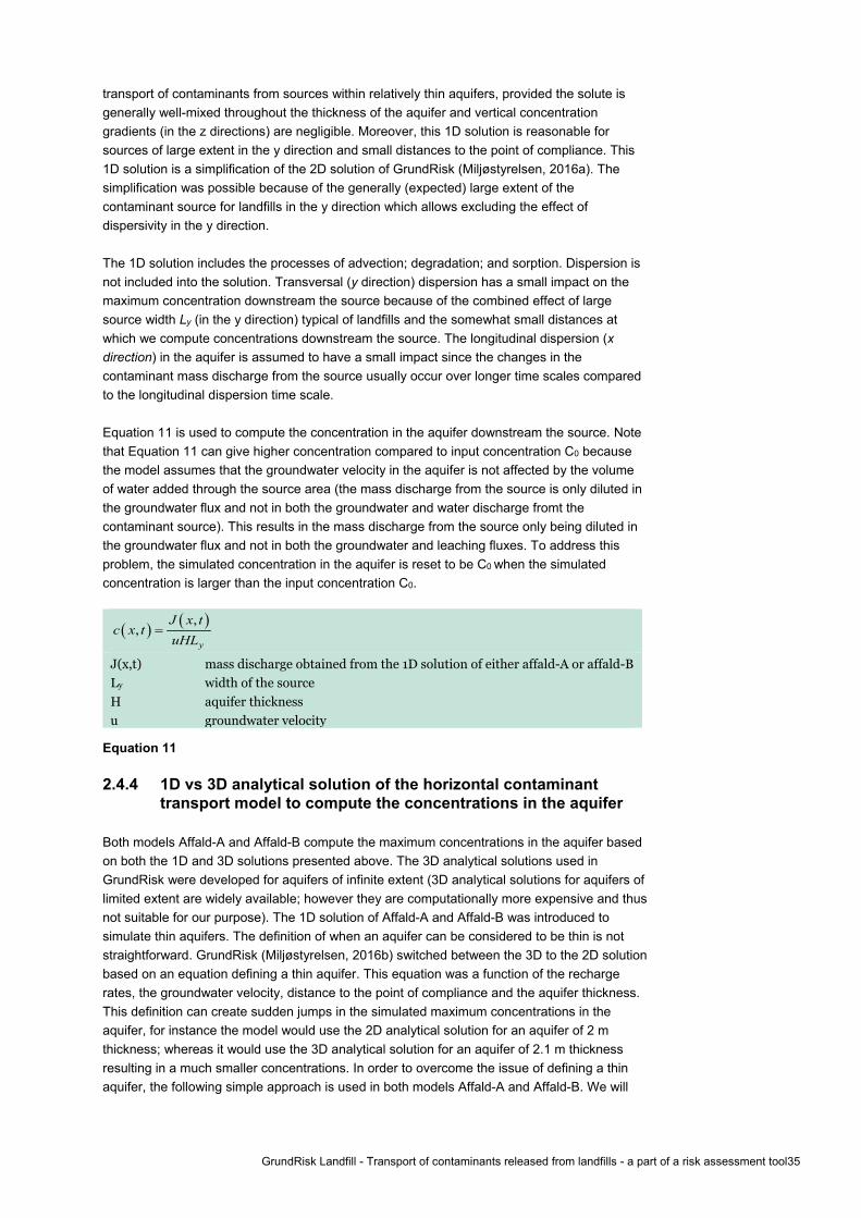
GrundRisk Landfill - Transport of contaminants released from landfills - a part of a risk assessment tool35
transport of contaminants from sources within relatively thin aquifers, provided the solute is generally well-mixed throughout the thickness of the aquifer and vertical concentration gradients (in the z directions) are negligible. Moreover, this 1D solution is reasonable for sources of large extent in the y direction and small distances to the point of compliance. This 1D solution is a simplification of the 2D solution of GrundRisk (Miljøstyrelsen, 2016a). The simplification was possible because of the generally (expected) large extent of the contaminant source for landfills in the y direction which allows excluding the effect of dispersivity in the y direction. The 1D solution includes the processes of advection; degradation; and sorption. Dispersion is not included into the solution. Transversal (y direction) dispersion has a small impact on the maximum concentration downstream the source because of the combined effect of large source width Ly (in the y direction) typical of landfills and the somewhat small distances at which we compute concentrations downstream the source. The longitudinal dispersion (x direction) in the aquifer is assumed to have a small impact since the changes in the contaminant mass discharge from the source usually occur over longer time scales compared to the longitudinal dispersion time scale. Equation 11 is used to compute the concentration in the aquifer downstream the source. Note that Equation 11 can give higher concentration compared to input concentration C0 because the model assumes that the groundwater velocity in the aquifer is not affected by the volume of water added through the source area (the mass discharge from the source is only diluted in the groundwater flux and not in both the groundwater and water discharge fromt the contaminant source). This results in the mass discharge from the source only being diluted in the groundwater flux and not in both the groundwater and leaching fluxes. To address this problem, the simulated concentration in the aquifer is reset to be C0 when the simulated concentration is larger than the input concentration C0.
( ) ( ),,
y
J x tc x t
uHL=
J(x,t) mass discharge obtained from the 1D solution of either affald-A or affald-B Ly width of the source H aquifer thickness u groundwater velocity
Equation 11 2.4.4 1D vs 3D analytical solution of the horizontal contaminant
transport model to compute the concentrations in the aquifer Both models Affald-A and Affald-B compute the maximum concentrations in the aquifer based on both the 1D and 3D solutions presented above. The 3D analytical solutions used in GrundRisk were developed for aquifers of infinite extent (3D analytical solutions for aquifers of limited extent are widely available; however they are computationally more expensive and thus not suitable for our purpose). The 1D solution of Affald-A and Affald-B was introduced to simulate thin aquifers. The definition of when an aquifer can be considered to be thin is not straightforward. GrundRisk (Miljøstyrelsen, 2016b) switched between the 3D to the 2D solution based on an equation defining a thin aquifer. This equation was a function of the recharge rates, the groundwater velocity, distance to the point of compliance and the aquifer thickness. This definition can create sudden jumps in the simulated maximum concentrations in the aquifer, for instance the model would use the 2D analytical solution for an aquifer of 2 m thickness; whereas it would use the 3D analytical solution for an aquifer of 2.1 m thickness resulting in a much smaller concentrations. In order to overcome the issue of defining a thin aquifer, the following simple approach is used in both models Affald-A and Affald-B. We will

36 GrundRisk Landfill - Transport of contaminants released from landfills - a part of a risk assessment tool
compute the maximum concentrations in the aquifer based on both the 1D and 3D solutions presented above and the most conservative solution is the one chosen. In this way we implicitly assume that if the chosen solution is the 1D then the aquifer is assumed to be a thin aquifer (and vice versa). Moreover, we avoid sudden jumps of simulated concentrations due to the choice of the 1D or 3D solution. 2.4.5 Solution of multiple spatially distributed landfill units Figure 10 shows that a landfill can be comprised of several different units that can have different contaminant concentrations C0(t), water discharges Q0(t) and transport distances. This section describes how the model computes the maximum concentrations in the aquifer resulting from multiple spatially distributed landfill units. Because the solute-transport equations are linear partial-differential equation we can use the superposition principle (section 2.4.1) to sum up the contributions from different spatially distributed single landfill units.
(a) Model Affald-A
(b) Model Affald-B
Figure 10. Contaminant transport from landfills comprised of multiple spatially distributed units with different input geometries, concentrations, leachate and transport distances.
In the case of a single landfill unit source, the timing and location of the maximum concentration of the contaminant plume in the aquifer is easily found: the maximum concentration in the aquifer is found at the center of the plume (that is known) and the model will compute the concentration time series at the center of the plume in order to find the timing when the maximum concentration occurs. However, in the case of multiple spatially distributed sources, the plume resulting from the spatial and temporal superposition of multiple spatially distributed sources can have a complex 3D shape that changes over time. To find the maximum concentration in the case of multiple spatially distributed sources the model will therefore need to compute the time variation of a 3D contaminant plume and this is computationally expensive since the concentration distribution of each landfill unit over a z-y plane at a given x (usually at the point of compliance) needs to be computed at each time step (this can easily take several hours). Instead, a simplified model approach is used in order to significantly reduce the computational time and obtain a reasonable and conservative approximation of the maximum concentration of the complex contaminant plume. The model includes 3 different steps in order to find/compute the maximum concentration of a 3D time-dependent contaminant plume resulting from the superposition of multiple spatially distributed sources: 1) find the maximum concentration of the contaminant plume in the y direction; 2) find the maximum concentration of the contaminant plume in the z direction; and 3) find the maximum concentration of the contaminant plume in the time domain.
Top of the aquifer
Terrain level
Contaminantplume
AquiferGroundwater flow direction
Point of compliance
Satu
rate
d/
unsa
tura
ted
zone
Landfill areaCon
tam
inan
t flu
x
xy
z
Unit I
Unit II
Satu
rate
dzo
ne
Top of the aquifer
Terrain level
Contaminantplume
Aquifer
Groundwater flow direction
Point of compliance
z
x
Satu
rate
dzo
ne
Unit I
yUnit II

GrundRisk Landfill - Transport of contaminants released from landfills - a part of a risk assessment tool37
Table 3 summarizes the model approach used to find the maximum concentration in the aquifer in the case of multiple spatially distributed landfill units.
Table 3. Model approach used to find the total maximum concentration in the aquifer in the case of multiple spatially distributed units within the same landfill.
In the y direction - If the sources overlap then the total maximum concentration equals the sum of the maximum concentrations from each landfill unit source - If the sources do not overlap then the total maximum equals the highest maximum concentration among the single landfill unit sources
In the z direction the total maximum concentration equals the sum of the maximum concentrations from each landfill unit source
In the time domain
The total maximum concentration in time is found from the total concentration distribution. The total concentration distribution is computed by summing up the concentrations as function of time from each landfill unit source
Step 1. Find the maximum in the y direction The concentration distribution variation in the y direction is related to (i) the spatial distribution of the different sources in the y direction, (ii) the hydrodynamic dispersion in the y direction, (iii) the geometry of the sources and (iv) the traveling distances downstream the sources. Figure 11 shows two examples of the concentration distribution in the y direction resulting from two different sources that overlap in one case and do not overlap in the other. The results shows that the concentration resulting from each unit has a flat constant front in the y direction because of the large extent of the landfill units in the y direction and the limited distances (compared to the source width) at which we compute the concentrations. Figure 11a shows that the total maximum concentration (gray dots/lines) is the same as the maximum concentration of Unit 2 (blue line) in the case the sources do not overlap; whereas the total maximum concentration is the sum of the two maximum concentrations of Unit 1 and 2 in the case the source overlap (Figure 11b). Based on the above discussion the model computes the maximum concentration as:
- If the sources do not overlap in the y direction the maximum concentration is the maximum concentration resulting from either Unit 1 or Unit 2.
- If the sources overlap in the y direction the maximum concentration is the sum of the maximum concentration resulting from both Unit 2 and Unit 3.
The same concept applies in the case of more than two sources. This approach can overestimate the total concentration in the case the sources slightly overlap in the y direction.

38 GrundRisk Landfill - Transport of contaminants released from landfills - a part of a risk assessment tool
Figure 11. Example of 2 different spatial distributions of the sources in the y direction together with the resulting concentrations at 100 m downstream of unit 2. (a) The sources do not overlap in the y direction; (b) the sources overlap in the y direction. The red lines show the concentration results from unit 1, the blue lines show the concentration results of unit 2, and the gray dots/lines show the total concentration resulting from the superposition of the 2 contributions.
Step 2. Find the maximum in the z direction The concentration distribution in the z direction is related to Ii) the spatial distribution of the different sources in the x direction, (ii) the hydrodynamic dispersion in the z direction, (iii) the geometry of the sources and (iv) the traveling distances downstream the sources. Figure 12 shows two examples of the concentration distribution in the z direction resulting from two different sources that are located at different x locations. The results show that the center of the plume at the point of compliance has travelled downward in the z direction due to the recharge on top of the aquifer. The figure shows that the total maximum concentrations (gray lines) are higher than the resulting concentration from each unit if the centers of the plumes are close to each other (Figure 12a); whereas, the total concentrations are similar to the resulting concentration from each unit if the centers of the plumes are far from each other (Figure 12b). As mentioned above, computing the distribution of concentrations in the z direction is computationally expensive. Moreover, the center of the plume is calculated in a simplified way assuming a constant horizontal groundwater velocity (model input) and a constant vertical velocity (that is calculated from the groundwater recharge) that pushes the plume downward downstream the source. This simple approach that assumes a constant vertical velocity can be violated, for instance if the bottom of the aquifer is confined by an impermeable layer, then the vertical velocities decrease almost linearly over depth (zero at the bottom of the aquifer). The contaminant plume can also travel below another source that can have a different vertical leachate flow than the groundwater recharge. Moreover, groundwater flow velocities in the aquifer can significantly vary within few hundred meters and this becomes relevant since spatially distributed sources in a landill can easily reach a horizontal span of about 500 m from the most upstream source point to the point of compliance (see Figure 4). Based on the above discussion the model computes the maximum concentration as:
- The total maximum concentration is the sum of the maximum concentrations from each unit.
Concentration [mg/L]x
y
Unit 1
Uni
t 2
(a) Sources do not overlap in they direction
(b) Sources overlap in the y direction
Concentration [mg/L]
Unit 1
Uni
t 2
Unit 1Unit 2Total

GrundRisk Landfill - Transport of contaminants released from landfills - a part of a risk assessment tool39
This overestimates the total concentration since the locations of the maximums is very unlikely to match. Since we know the maximum concentration from each source we can estimate the maximum overestimation factor. For instance, if there are 2 concentration distributions (from 2 different sources), one having 100 mg/L as maximum concentration and the other 70 mg/L, the total maximum concentration would be 170 mg/L as we assume that the centers of the 2 plumes coincide. However if the center of the plumes would be far apart (similar to Figure 12b) the total maximum concentration would be 100 mg/L. Thus we can say that the computed total maximum concentration can be overestimated by 70% due the uncertainty about the vertical distribution of the plume (in the z direction).
Figure 12. (note that the z direction is exaggerated for illustration purposes). Examples of 2 different spatial distributions of the sources in the x direction together with the resulting concentrations. The orange lines show the concentration results from the upstream source, the blue lines show the concentration results from the downstream source, and the gray dots/lines show the total concentration resulting from the superposition of the 2 contributions.
Step 3. Find the maximum in time The concentration distribution as a function of time at a control point in the aquifer is related to the spatial distribution of the different sources in the x direction; to the hydrodynamic dispersion in the x direction; to the retardation factor; to the contaminant mass discharge input; to the geometry of the sources and to the traveling distances downstream the sources. Figure 13 shows an example of the concentration distribution as a function of time resulting from 2 different sources that are located at different x locations. The results show that the maximum concentrations from the 2 different sources occur at different times. The figure shows that the total maximum concentrations (gray lines) are higher than the resulting concentration from each unit. Based on the above the model computes the total maximum concentration by summing up the concentrations as function of time from each source.
Concentration [mg/L]
x
z
(a) Concentrations overlap in the z direction
(b) Concentrations do not overlap in the z direction
PoCsmall PoC
Concentration [mg/L]
Unit 1Unit 2Total
large
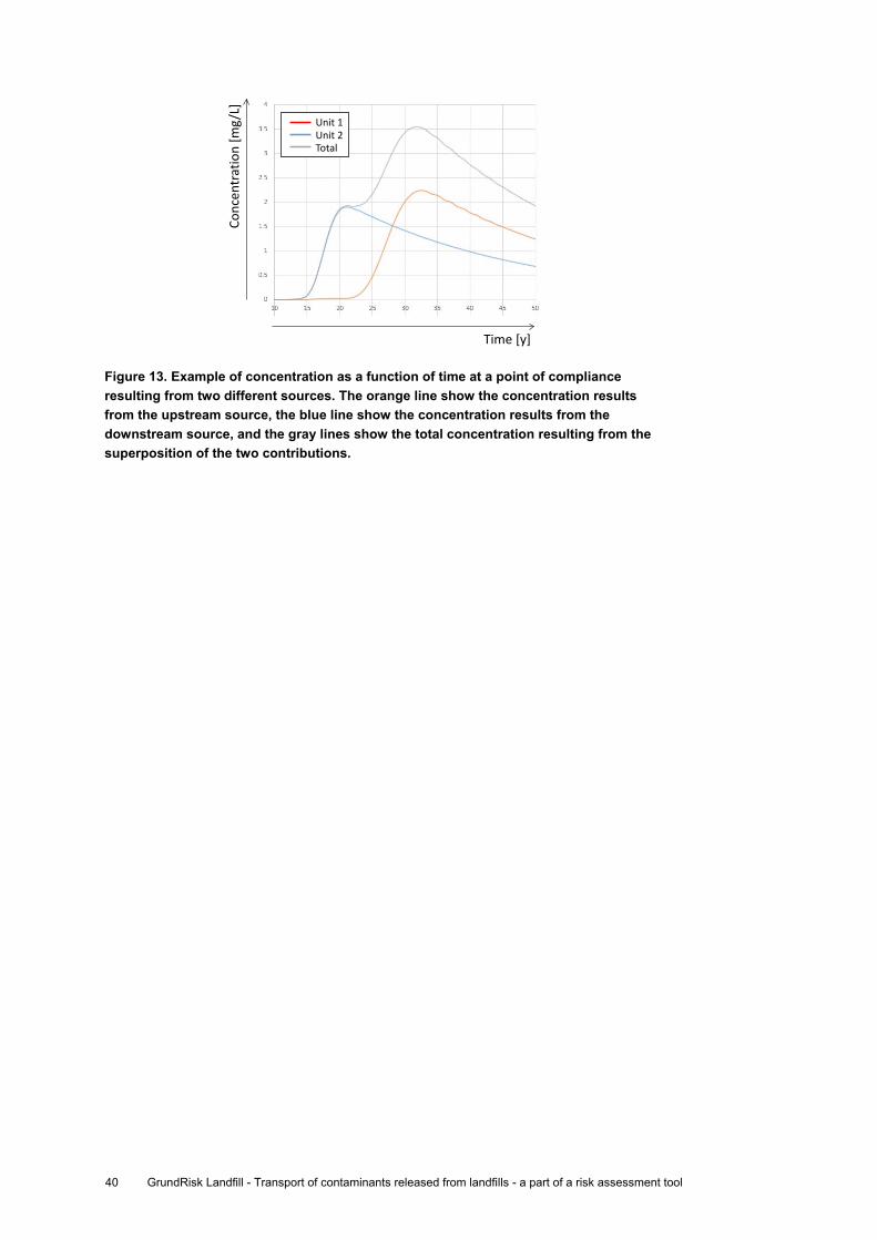
40 GrundRisk Landfill - Transport of contaminants released from landfills - a part of a risk assessment tool
Figure 13. Example of concentration as a function of time at a point of compliance resulting from two different sources. The orange line show the concentration results from the upstream source, the blue line show the concentration results from the downstream source, and the gray lines show the total concentration resulting from the superposition of the two contributions.
Conc
entr
atio
n [m
g/L]
Time [y]
Unit 1Unit 2Total

GrundRisk Landfill - Transport of contaminants released from landfills - a part of a risk assessment tool41
3. Model applications
This chapter presents an application of the models to three different landfills in Denmark. The landfills represent controlled and uncontrolled landfills or landfill sections managed under different legislation, regulatory framework and authorities as described in the introduction. The purpose of the model applications were to demonstrate the new GrundRisk Landfill model capabilities and in particular illustrate the main issues and challenges when modelling contaminant transport from landfills. It should be noted that the application did not aim to compare the results with actual data as this is beyond the scope of the report. The three landfills were chosen in order to illustrate a range of model applications. The first two landfills are comprised of several different landfill units, while the third consists of only a single landfill unit. Some of the considered units have a membrane and a leachate control system whereas others are without (uncontrolled). Two of the landfills are above the groundwater table and are simulated using model Affald-A while the other landfill is partly below the groundwater table and is simulated using the model Affald-B. The data used for the three landfills come from historical reports written over a 25 years’ period. The reports showed inconsistencies in descriptions of the hydrology, landfills, leachate composition and hydrogeology in the area. This is a big challenge. However, the examples and the data available are typical for older Danish landfills, so this chapter also discusses the assumptions and simplifications required in order to use the models for risk assessment. Each example provides a description of the landfill; the input data obtained by the Source term model (Miljøstyrelsen, 2018a,b); the model parameters and the model results. The examples are based on historical data, so currently observed contaminations in the aquifer can be very different because recent investigations and remedial actions may not have been considered. 3.1 Tandskov landfill. Application of the model ‘Affald-A’ Affaldscenter Tandskov is a landfill located close to Silkeborg. The landfill covers an area of approximately 25 hectares and has different landfill units (Afdelinger and Fyldplads, see Figure 14). Unit 1 is an uncontrolled unit with leachate entering the underlying environment; Units 2-4 have membrane and leachate collection systems, however with a leak detected in the membrane of Unit 3. The landfill waste is located in the unsaturated zone tens of meters above the groundwater table. Several site investigations have been conducted and have shown that contaminants have reached and spread into the groundwater aquifer underneath the landfill (Aarhus Amt, 2006).

42 GrundRisk Landfill - Transport of contaminants released from landfills - a part of a risk assessment tool
Figure 14. Plan view of the Tandskov landfill. Figure from Aarhus Amt, 2006.
3.1.1 Geology and hydrogeology Affaldscenter Tandskov is located in the unsaturated zone on a sandy and gravel soil with clay lenses. Figure 15 shows a geological cross section of the area. The groundwater table in the area around Affaldscenter Tandskov is located at approximately 50 m above sea level (Aarhus Amt, 2006). The average thickness of the unconfined aquifer is estimated to be about 15 m and the aquifer is assumed to be confined by the continuous clay layer shown in Figure 15. Figure 16 shows the groundwater equipotential lines in the area and the groundwater flow streamlines. The groundwater flows towards north-west and hydraulic gradients are shown to become steeper downstream the landfill.
Figure 15. Geological cross section (left side=north-west; left side=south-east) showing the sand layer (white), the clay (diagonal black lines) and the landfill area (vertical black lines). The figure also shows the approximate position of the groundwater table and an approximation of the thickness of the aquifer. Also, the depression on the left side of the figure represents the stream flowing west of the landfill. Figure modified from Aarhus Amt (2006).

GrundRisk Landfill - Transport of contaminants released from landfills - a part of a risk assessment tool43
The blue arrow of Figure 16 shows the horizontal groundwater flow direction used in the Source term model. Each landfill unit is assigned a rectangular area (of length Lx and width Ly) aligned with the groundwater flow direction. The hydraulic gradient is 0.011 based on the equipotential map on Figure 16. The porosity of the sand is assumed to be 0.3 and the hydraulic conductivity 0.0001 m/s (Carl Bro, 2007). This gives a groundwater velocity of 116 m/y. The groundwater equipotential map shows a significant spatial variation of the groundwater gradients that makes the groundwater velocity estimation uncertain. The vertical leachate flux below some of the units of the landfill was estimated to be 350-400 mm/y (Carl Bro, 2007). The groundwater recharge in the area (the model uses this value to push the contaminant plume downward downstream the landfill) is 110 mm/y according to the DK-Model (Højberg et al., 2015) and 488 mm/y according to JAGG(JAGG 2.0).
Figure 16. Groundwater equipotential map of the Tandskov area. The blue arrow shows the location where we estimated the groundwater flow velocity. The direction of the arrow is parallel to the Source term model estimation of the groundwater flow direction. Figure modified from Aarhus Amt, 2006. 3.1.2 Description of the source and the data from Source term model The input concentration and water discharge/ leachate through the bottom of each landfill unit was provided by the Source term model. The input concentration was provided for several compounds and Figure 17a shows an example of the input concentration of chloride from Unit 1 (Afdeling 1). The time period of the input concentration time series is 500 years. Figure 17b shows the water discharge from Unit 1. The water discharge is in this case constant over the 500 years period. The geometry of the source area is assumed to be rectangular and aligned with the groundwater flow direction. The source length and width and the spatial location of the source areas were provided by the Source term model. Chloride and ammonium were selected as “model compounds” as they are present in high concentrations, are represented by two different source functions (leaching curves, as determined by the Source term model),
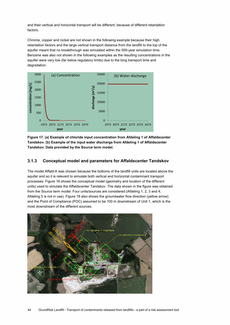
44 GrundRisk Landfill - Transport of contaminants released from landfills - a part of a risk assessment tool
and their vertical and horizontal transport will be different, because of different retardation factors. Chrome, copper and nickel are not shown in the following example because their high retardation factors and the large vertical transport distance from the landfill to the top of the aquifer meant that no breakthrough was simulated within the 500-year simulation time. Benzene was also not shown in the following examples as the resulting concentrations in the aquifer were very low (far below regulatory limits) due to the long transport time and degradation.
Figure 17. (a) Example of chloride input concentration from Afdeling 1 of Affaldscenter Tandskov. (b) Example of the input water discharge from Afdeling 1 of Affaldscenter Tandskov. Data provided by the Source term model.
3.1.3 Conceptual model and parameters for Affaldscenter Tandskov The model Affald-A was chosen because the bottoms of the landfill units are located above the aquifer and so it is relevant to simulate both vertical and horizontal contaminant transport processes. Figure 18 shows the conceptual model (geometry and location of the different units) used to simulate the Affaldscenter Tandskov. The data shown in the figure was obtained from the Source term model. Four units/sources are considered (Afdeling 1, 2, 3 and 4; Afdeling 5 is not in use). Figure 18 also shows the groundwater flow direction (yellow arrow) and the Point of Compliance (POC) assumed to be 100 m downstream of Unit 1, which is the most downstream of the different sources.
0
500
1000
1500
2000
2500
3000
1973 2073 2173 2273 2373 2473
conc
entr
atio
n [m
g/L]
year
(a) Concentration
0
5000
10000
15000
20000
25000
1973 2073 2173 2273 2373 2473
disc
harg
e [m
3 /y]
year
(b) Water discharge
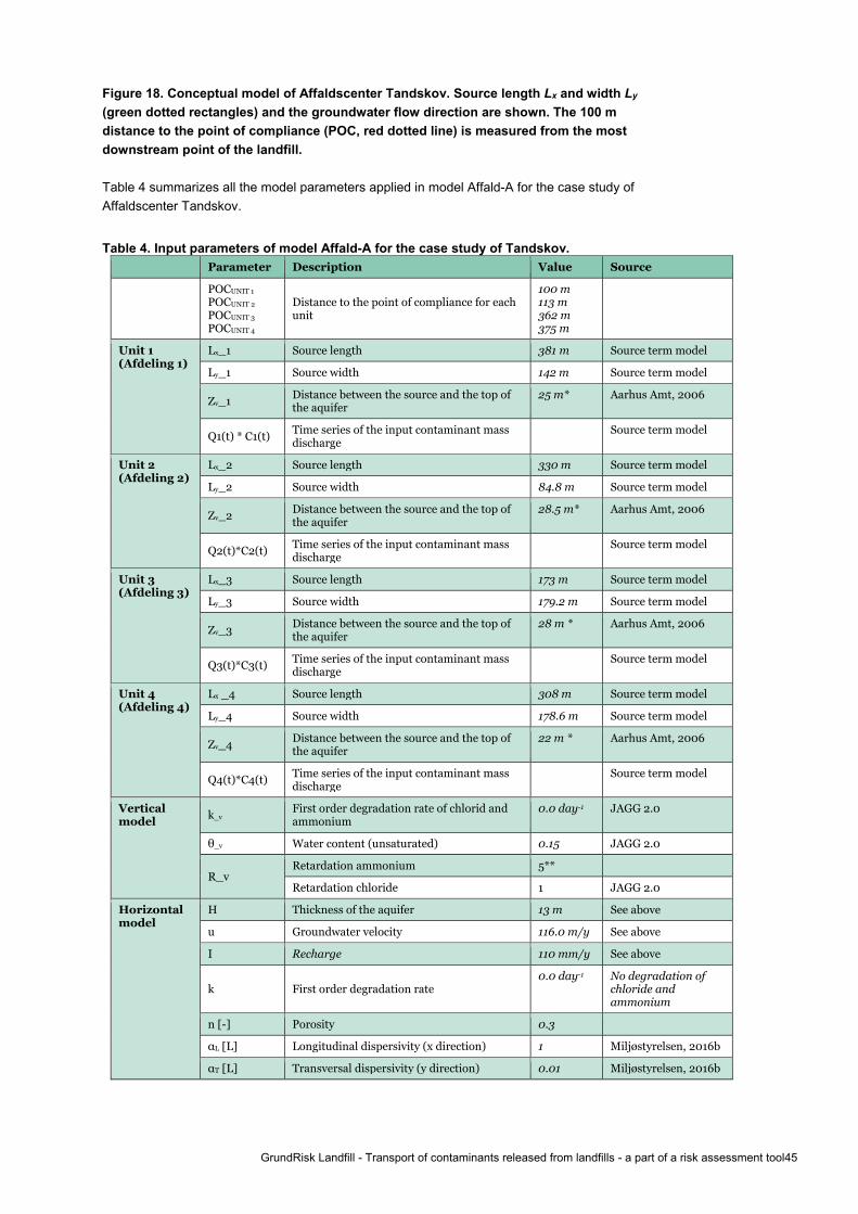
GrundRisk Landfill - Transport of contaminants released from landfills - a part of a risk assessment tool45
Figure 18. Conceptual model of Affaldscenter Tandskov. Source length Lx and width Ly (green dotted rectangles) and the groundwater flow direction are shown. The 100 m distance to the point of compliance (POC, red dotted line) is measured from the most downstream point of the landfill. Table 4 summarizes all the model parameters applied in model Affald-A for the case study of Affaldscenter Tandskov.
Table 4. Input parameters of model Affald-A for the case study of Tandskov. Parameter Description Value Source
POCUNIT 1
POCUNIT 2
POCUNIT 3
POCUNIT 4
Distance to the point of compliance for each unit
100 m 113 m 362 m 375 m
Unit 1 (Afdeling 1)
Lx_1 Source length 381 m Source term model
Ly_1 Source width 142 m Source term model
Zv_1 Distance between the source and the top of the aquifer
25 m* Aarhus Amt, 2006
Q1(t) * C1(t) Time series of the input contaminant mass discharge
Source term model
Unit 2 (Afdeling 2)
Lx_2 Source length 330 m Source term model
Ly_2 Source width 84.8 m Source term model
Zv_2 Distance between the source and the top of the aquifer
28.5 m* Aarhus Amt, 2006
Q2(t)*C2(t) Time series of the input contaminant mass discharge
Source term model
Unit 3 (Afdeling 3)
Lx_3 Source length 173 m Source term model
Ly_3 Source width 179.2 m Source term model
Zv_3 Distance between the source and the top of the aquifer
28 m * Aarhus Amt, 2006
Q3(t)*C3(t) Time series of the input contaminant mass discharge
Source term model
Unit 4 (Afdeling 4)
Lx _4 Source length 308 m Source term model
Ly_4 Source width 178.6 m Source term model
Zv_4 Distance between the source and the top of the aquifer
22 m * Aarhus Amt, 2006
Q4(t)*C4(t) Time series of the input contaminant mass discharge
Source term model
Vertical model k_v
First order degradation rate of chlorid and ammonium
0.0 day-1 JAGG 2.0
θ_v Water content (unsaturated) 0.15 JAGG 2.0
R_v Retardation ammonium 5**
Retardation chloride 1 JAGG 2.0
Horizontal model
H Thickness of the aquifer 13 m See above
u Groundwater velocity 116.0 m/y See above
I Recharge 110 mm/y See above
k First order degradation rate 0.0 day-1 No degradation of
chloride and ammonium
n [-] Porosity 0.3
αL [L] Longitudinal dispersivity (x direction) 1 Miljøstyrelsen, 2016b
αT [L] Transversal dispersivity (y direction) 0.01 Miljøstyrelsen, 2016b

46 GrundRisk Landfill - Transport of contaminants released from landfills - a part of a risk assessment tool
αV [L] Vertical dispersivity (z direction) 0.005 Miljøstyrelsen, 2016b
R Retardation ammonium 5**
Retardation chloride 1 JAGG 2.0
* Afdeling 1 has a fill depth of 10 m; Afdeling 2 of 6.5 m; Afdeling 3 of 7 m and Afdeling 4 of 13 m (Aarhus Amt, 2006). Assuming an average terrain elevation of 85 m, that the fill is not above terrain level and a groundwater head at 50 m (above sea level) we estimated the vertical travel distance from the bottom of the landfill unit to the top of the unconfined groundwater table. ** The retardation factor for ammonium was chosen from literature (Christensen et al., 2001) assuming that ammonium retardation can be described as a sorption process (ammonium is undergoing cation exchange, which is a non-linear process). Ammonium can also be transformed to nitrate or other nitrogen species in the aquifer. This is not included, but the worst case concentrations of nitrate (from ammonium) can be estimated from a stoichiometric conversion of ammonium to nitrate. 1 mol of ammonium is assumed to be converted to 1 mol nitrate or 1 mg/L of ammonium will be converted to 3,44 mg/l of nitrate.
3.1.4 Model results for Unit 1 (Afdeling 1) of Affaldscenter Tandskov This section shows the model results obtained assuming that the landfill only consists of a single unit (Afdeling 1). This was simply done for an easier presentation and discussion of the model results. This section is divided into two subsections because different model are used to compute the concentration and the mass discharge as a function of time at the point of compliance. The ‘Contaminant water concentrations’ describes the concentrations downstream Unit 1, whereas the ‘Contaminant mass discharge’ describes the contaminant mass discharge downstream of Unit 1. Contaminant water concentrations Figure 19 shows the simulation results obtained using the model Affald-A applied to Affaldscenter Tandskov Afdeling 1 (Unit 1). The simulation results show similar concentration patterns for both ammonium and chloride (the compounds chosen in this example). The concentrations at the source show an exponential decrease in time. The concentration distributions after vertical transport show the same patterns as the source concentrations, but have been shifted in time due to the travel time through the 25 m thick unsaturated sand layer. The time shift is much larger for ammonium because of the 5 times higher retardation factor which slows down the transport processes due to higher sorption. The concentration time series after vertical transport is similar to the source because the vertical model does not include dispersion. Because ammonium and chloride do not degrade and because dispersion is ignored, the maximum concentrations after vertical transport are the same as the maximum concentrations at the source. The concentration of chloride in the aquifer resulting from the 3D model shows a flat peak concentration. This is because the 3D analytical solution calculated higher maximum chloride concentrations in the aquifer compared to the maximum concentration inputs. Therefore the model (as explained in section 2.2.3) cuts off all the concentration that are higher than the maximum input concentration since they are physically unrealistic. This happens because the 3D model both underestimates dilution of inflowing leachate as only the contaminant mass discharge is included (and not water) and vertical advection due to the vertical leachate velocity is not included as explained in Section 2.2.3. The peak concentration in the aquifer is just few years later than the peak input concentrations (after vertical transport) because of the relatively high groundwater velocity and the relatively short horizontal distance to the point of compliance. The concentration of ammonium in the aquifer resulting from the 3D model shows a lower peak concentration compared to the input peak concentration and a longer time shift compared to the chloride breakthrough curve due to the higher retardation factor. A higher retardation factor makes transport velocities slower and this combined with the horizontal extent of the source Lx makes the concentrations at the point of compliance smoother in time.
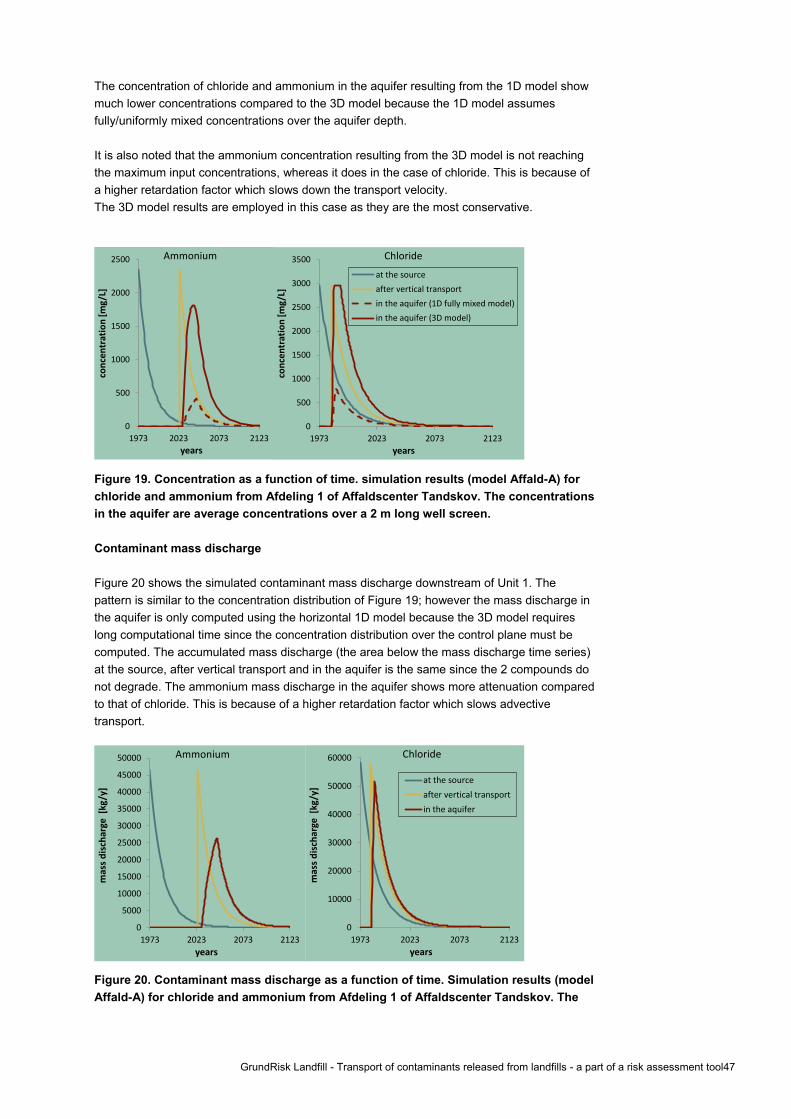
GrundRisk Landfill - Transport of contaminants released from landfills - a part of a risk assessment tool47
The concentration of chloride and ammonium in the aquifer resulting from the 1D model show much lower concentrations compared to the 3D model because the 1D model assumes fully/uniformly mixed concentrations over the aquifer depth. It is also noted that the ammonium concentration resulting from the 3D model is not reaching the maximum input concentrations, whereas it does in the case of chloride. This is because of a higher retardation factor which slows down the transport velocity. The 3D model results are employed in this case as they are the most conservative.
Figure 19. Concentration as a function of time. simulation results (model Affald-A) for chloride and ammonium from Afdeling 1 of Affaldscenter Tandskov. The concentrations in the aquifer are average concentrations over a 2 m long well screen. Contaminant mass discharge Figure 20 shows the simulated contaminant mass discharge downstream of Unit 1. The pattern is similar to the concentration distribution of Figure 19; however the mass discharge in the aquifer is only computed using the horizontal 1D model because the 3D model requires long computational time since the concentration distribution over the control plane must be computed. The accumulated mass discharge (the area below the mass discharge time series) at the source, after vertical transport and in the aquifer is the same since the 2 compounds do not degrade. The ammonium mass discharge in the aquifer shows more attenuation compared to that of chloride. This is because of a higher retardation factor which slows advective transport.
Figure 20. Contaminant mass discharge as a function of time. Simulation results (model Affald-A) for chloride and ammonium from Afdeling 1 of Affaldscenter Tandskov. The
0
500
1000
1500
2000
2500
3000
3500
1973 2023 2073 2123
conc
entr
atio
n [m
g/L]
years
Chloride
at the sourceafter vertical transportin the aquifer (1D fully mixed model)in the aquifer (3D model)
0
500
1000
1500
2000
2500
1973 2023 2073 2123
conc
entr
atio
n [m
g/L]
years
Ammonium
0
10000
20000
30000
40000
50000
60000
1973 2023 2073 2123
mas
s dis
char
ge [
kg/y
]
years
Chloride
at the sourceafter vertical transportin the aquifer
0
5000
10000
15000
20000
25000
30000
35000
40000
45000
50000
1973 2023 2073 2123
mas
s dis
char
ge [
kg/y
]
years
Ammonium
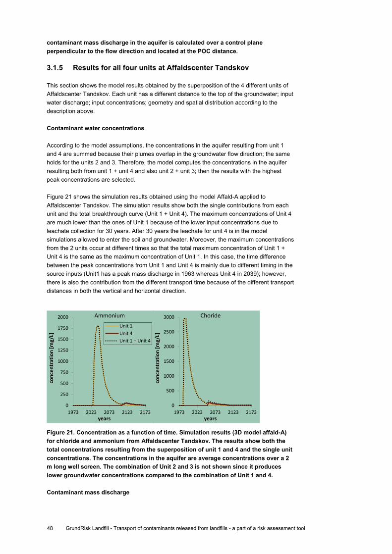
48 GrundRisk Landfill - Transport of contaminants released from landfills - a part of a risk assessment tool
contaminant mass discharge in the aquifer is calculated over a control plane perpendicular to the flow direction and located at the POC distance. 3.1.5 Results for all four units at Affaldscenter Tandskov This section shows the model results obtained by the superposition of the 4 different units of Affaldscenter Tandskov. Each unit has a different distance to the top of the groundwater; input water discharge; input concentrations; geometry and spatial distribution according to the description above. Contaminant water concentrations According to the model assumptions, the concentrations in the aquifer resulting from unit 1 and 4 are summed because their plumes overlap in the groundwater flow direction; the same holds for the units 2 and 3. Therefore, the model computes the concentrations in the aquifer resulting both from unit 1 + unit 4 and also unit 2 + unit 3; then the results with the highest peak concentrations are selected. Figure 21 shows the simulation results obtained using the model Affald-A applied to Affaldscenter Tandskov. The simulation results show both the single contributions from each unit and the total breakthrough curve (Unit 1 + Unit 4). The maximum concentrations of Unit 4 are much lower than the ones of Unit 1 because of the lower input concentrations due to leachate collection for 30 years. After 30 years the leachate for unit 4 is in the model simulations allowed to enter the soil and groundwater. Moreover, the maximum concentrations from the 2 units occur at different times so that the total maximum concentration of Unit 1 + Unit 4 is the same as the maximum concentration of Unit 1. In this case, the time difference between the peak concentrations from Unit 1 and Unit 4 is mainly due to different timing in the source inputs (Unit1 has a peak mass discharge in 1963 whereas Unit 4 in 2039); however, there is also the contribution from the different transport time because of the different transport distances in both the vertical and horizontal direction.
Figure 21. Concentration as a function of time. Simulation results (3D model affald-A) for chloride and ammonium from Affaldscenter Tandskov. The results show both the total concentrations resulting from the superposition of unit 1 and 4 and the single unit concentrations. The concentrations in the aquifer are average concentrations over a 2 m long well screen. The combination of Unit 2 and 3 is not shown since it produces lower groundwater concentrations compared to the combination of Unit 1 and 4. Contaminant mass discharge
0
250
500
750
1000
1250
1500
1750
2000
1973 2023 2073 2123 2173
conc
entr
atio
n [m
g/L]
years
Ammonium
Unit 1Unit 4Unit 1 + Unit 4
0
500
1000
1500
2000
2500
3000
1973 2023 2073 2123 2173
conc
entr
atio
n [m
g/L]
years
Choride

GrundRisk Landfill - Transport of contaminants released from landfills - a part of a risk assessment tool49
Figure 22 shows the simulation results obtained using the model Affald-A applied to Affaldscenter Tandskov. The simulation results show both the single contributions from each unit and the total breakthrough curve. The maximum mass discharge from each unit occurs at different times because of different transport times due to both different vertical and horizontal transport distances and different periods of the input leachate time series.
Figure 22. Contaminant mass discharge as a function of time (the mass discharge of unit 2 is small compared to the others and thus it is not visible in the large vertical scale of the graphs). Simulation results for chloride and ammonium from Affaldscenter Tandskov (model Affald-A). The results show both the total concentrations resulting from the superposition of unit 1 and 4 and the single unit concentrations. The concentrations in the aquifer are average concentrations over a 2 m long well screen. 3.1.6 Conclusion of the model Affald-A application to the landfill of
Tandskov The results of the model Affald-A application to the landfill of Tandskov showed the following:
- Only the concentrations in the aquifer resulting from the units that do overlap in the groundwater flow direction sum up with each other. - The maximum concentrations of ammonium in the aquifer are slightly reduced whereas the maximum concentrations of chloride in the aquifer equal the maximum source concentrations. Such small reductions of maximum concentrations in the aquifer are due to the zero degradation of the compounds, the large areas of the units, the relatively short distance to the POC and the large contaminant mass discharge from the units (in such conditions dilution and dispersion have a small effect on the concentrations downstream the landfill). - The maximum concentrations in the aquifer resulting from the same compound coming from different units occur at different times because of the different horizontal transport distances to the POC; vertical transport distances to the top of the aquifer; vertical velocities due to different leachate velocities; and source concentrations and leachate time series. - The maximum peak concentration of chloride in the aquifer (Figure 19) showed a flat peak. This means that the 3D analytical solution of Affald-A produced concentrations that were higher than the maximum input concentrations and therefore the model Affald-A cut-off all the aquifer concentrations which are higher than the maximum input concentrations. This occurs because of the model assumption that the groundwater flow is horizontal and not affected by the water discharge coming from the landfill. The exclusion of the additional water coming from the landfill and the consequent vertical downward velocities in the aquifer below the landfill produce an overestimation of the aquifer concentrations. For substances with
0
5000
10000
15000
20000
25000
30000
35000
40000
1967 2017 2067 2117 2167
mas
s dis
char
ge [
kg/y
]
years
Ammonium
0
10000
20000
30000
40000
50000
60000
70000
1967 2017 2067 2117 2167
mas
s dis
char
ge [
kg/y
]
years
Klorid
Unit 1Unit 2Unit 3Unit 4Total

50 GrundRisk Landfill - Transport of contaminants released from landfills - a part of a risk assessment tool
low sorption ability, it is reasonable that the concentration at the point of compliance is the same as that of the source because dilution and dispersion processes have little effect for such large source areas and short downstream distances. - The total mass discharge from the landfill is the sum of the single units’contributions. The contribution from each unit occurs at different periods of time. - Nickel, chrome and copper would not reach the POC within the 500 years simulation period because the high retardation factors would delay the breakthrough beyond the 500-year simulation time and due to the large vertical transport distance from the landfill to the top of the aquifer. - Benzene concentrations at the point of compliance were very low (much lower than quality criteria) because of the long transport times and high degradation rates.
3.2 Faaborg Landfill. Application of the model ‘Affald-B’ Faaborg Landfill is an old landfill that was operational in the period 1940-1975 in Faaborg. The area is now covered by buildings or is paved. Figure 23 shows the location of the landfill.,The landfill is close to Sundet that is a wetland/shallow lake. The landfill is assumed to be ‘uncontrolled’, meaning that neither a bottom membrane nor leachate collection system was installed. The landfill consists of two different compartments (reg.nr. 431-10 that is the most north of the two compartments shown in red in Figure 23 and reg.nr. 431-11). From the investigations in 1994 (Nielsen et al., 1994), it appears, that the actual delineation of the two parts of the landfill differs from the registered delineation, see Figure 23.
Figure 23. (left) Map of the Faaborg landfill (the red area), modified from Nielsen et al. (1994). The orange line represents the location (along Sundvejen) of the geological cross section shown in Figure 24. (right-top) 1999 arial photo of the Faaborg landfill and surroundings showing the construction works for the road "Sundvejen" in progress and initial rise of the waterlevel in "Sundet". (right-bottom) 2002 aerial photo of the Faaborg landfill and surroundings showing the final extent of "Sundet" after the water level reaching -1,1 m DVR.
B
A

GrundRisk Landfill - Transport of contaminants released from landfills - a part of a risk assessment tool51
3.2.1 Geology and hydrogeology Figure 24 shows the geological profile from Nielsen et al. (1994) along the road Sundvejen. The figure also shows the location of the landfill, the abstraction wells of the waterworks (‘Vandvaerk’), the wetland (‘Sundet’) and the road elevation of Sundvejen (‘Vejprofil’). The landfill lies on a low area (close to sea level) where the groundwater level of the upper aquifer is few meters below terrain level.
Figure 24. Geological cross section, modified after Nielsen et al. (1994) to show the location of the landfill (red area); the vertical extent of the landfill (the depth and the height of the landfill below and above terrain level is not to scale).
As shown in Figure 24 a thin layer of peat (about 1-2 m thick) and a thick (up to 10 m) buried valley filled with gyttja is present in the area below the landfill. There is a large aquitard made of clay till with lenses of meltwater sand. The whole area is underlain by a deeper aquifer consisting of meltwater sand, which is employed for drinking water abstraction. The groundwater flow directions and velocities are affected by the presence of abstraction wells both in the deeper aquifer (waterworks) and in the upper aquifer (pumping in the wetland of Sundet) (Nielsen et al., 1994). In 1994 and presumably until the time when the "Sundvejen" (a road) was realigned, the wetland north of the landfills ("Sundet") was kept dry by a drainage and pumping system keeping the groundwater level below the terrain level, i.e. below -1,5/-2,0 m DVR (1.5-2 m below mean sea level). Up until this point in time the hydraulic gradients in the deeper aquifer below the landfill were in the order of 2-3‰ (estimated from the groundwater potential map of Nielsen et al., 1994) and the groundwater flow direction was towards south-west (towards Faaborg Fjord). However, the groundwater flow direction could alter towards the waterworks depending on the abstraction rates. Nielsen et al. (1994) report a downward head gradient between the upper and the deeper aquifer; however, the exchange of water between the aquifers could change depending on the abstraction rates in the deeper aquifer. The flow direction in the upper aquifer below the landfill was found to be towards the waterworks (towards north-west of Figure 25) according to Naturforvaltningsproject (1993). However Nielsen et al. (1994) shows a groundwater potential map of the upper aquifer (see Figure 24) below the landfill with an overall groundwater flow direction towards north-east. Hydraulic gradients in the area were shown to vary in space and were approximately 5-25 ‰.
BA[m]
[m]
52 GrundRisk Landfill - Transport of contaminants released from landfills - a part of a risk assessment tool
After the year 2000 the water table in "Sundet" was allowed to rise. The aerial photo of Figure 23 (right-bottom) shows that in 2002 the water level was -1.1 m DVR. The water level has been maintained at that level since then by pumping from the existing pumping station shown in Figure 25. Also the pumping rate from the main waterworks in the deeper aquifer “Annexgården Vandværk” was reduced significantly, resulting in a new situation for the groundwater tables in the different aquifers. In Nielsen et al. (1994) the future groundwater potential in the deeper aquifer resulting from these changes was calculated and presented (see Fig 26). In Nielsen et al. (1994) other measures were discussed in connection with the realignment of "Sundvejen"; the rise of the water level and future environmental issues at the landfill area. This included a membrane installed on terrain of the now water covered parts of the landfill and a surface drainage system controlling the level of the near terrain water table in the landfill area. It is probable that a surface drainage system is installed. Assuming a linear decrease of the groundwater table close to the terrain between "Faaborg Sund", level +/- 0,0 m DVR, and the coastline of "Sundet", level -1,1 m DVR, the equipotential lines of Figure 26 may be outlined. Figure 26 suggests that the hydraulic gradients of the upper aquifer are approximately 1,5 ‰ towards northeast and that there is an upward gradient from the deeper aquifer towards the upper aquifer. Figure 24 shows a geological cross section in the area of the landfill and its surroundings. The hydraulic conductivity of the meltwater sand is 10-5 m/s; of gyttja and clay till is 10-6-10-9 m/s (Nielsen et al., 1994). The recharge was estimated to be 250 mm/y below green/unpaved areas and 20 mm/y below constructed areas (Nielsen et al., 1994). Nielsen et al. (1994) estimated that the hydraulic conductivity of the layers surrounding the landfill, ie. gyttja and peat, is approx. 10-6 m/s or lower, resulting a Darcy flow rate of approximately.q= k*I = 10-6 *0,0015 = 1,5*10-9 m/s = 0,05 m/y. This is a low flow rate and the term aquifer is somehow misleading for this layer of gyttja, mud and clay. It is likely, that the recharge into the area of the landfill may raise the water table relatively here, thus giving basis for estimating a higher groundwater gradient towards northeast. The main part of the terrain over the landfill is however situated at level +1,0 to +1,8 m DVR. As foundation of houses and paved areas typically is drained to approximately 0,8 m below terrain surface one may assume, that the overall water table will not exceed approx. level +1,0 m DVR, at the southwest edge of the landfill area. This results in a hydraulic gradient of approximately 9 ‰ and a Darcy flow rate of q= 0,28 m/y.

GrundRisk Landfill - Transport of contaminants released from landfills - a part of a risk assessment tool53
Figure 25. Equipotential map of the upper aquifer together with the location of the pumping station in Sundet. From Nielsen et al. (1994). The orange dashed circle show a rough approximate location of the landfill.
Figure 26. Groundwater equipotential lines of the deeper aquifer (Nielsen et al., 1994, Figure 5.5) and upper aquifer (estimated) in the landfill area. Deeper aquifer black lines; upper aquifer blue lines.
Pumping station

54 GrundRisk Landfill - Transport of contaminants released from landfills - a part of a risk assessment tool
3.2.2 Description of the landfill source The input concentration and water discharge from the different compartments of the landfill were provided by the Source term model. The input concentration was provided for several compounds and Figure 27 shows an example of input concentration and water leachate flux for Unit 1 of Faaborg. The time period of the input concentration time series is 500 years. The geometry of the source area is assumed to be rectangular and the source length and height were provided by the Source term model. Chloride and ammonium were selected as “model compounds” as they are present in high concentrations, represent two source functions (leaching curves) and their horizontal transport will be different, because of different retardation factors. Nickel was not shown in the following examples because of the high retardation factors which would delay the breakthrough beyond the 500-year simulation time mainly due to the large transport time due to the very low groundwater velocity. Benzene was also not shown in the following examples as the resulting concentrations at the POC would be too low to be reported and discussed.
Figure 27. Example of ammonium input concentration and water discharge from Unit 1 of Faaborg landfill (Mest nr. 431-10). These time series were provided by the Source term model.
3.2.3 Conceptual model and parameters The model ‘Landfill B. Multiple sources’ was chosen because the bottom of the different compartments of the landfill are located below the top of the upper aquifer. In this example we assumed that the contaminant transport occurs in the flow direction of the upper aquifer since we assumed an upward hydraulic gradient from the deeper to the upper aquifer. Figure 28 shows the conceptual model used to simulate the Faaborg landfill. Two different compartments are considered (431-10 and 431-11); the groundwater flow direction in the upper aquifer is towards north-east (aligned with the source geometries) and the Point of Compliance (POC) is assumed to be 100 m downstream the most downstream point of the different sources.
0
50
100
150
200
1940 2040 2140 2240 2340 2440
conc
entr
atio
n [m
g/L]
year
(a) Concentration
0
5000
10000
15000
20000
1940 2040 2140 2240 2340 2440
disc
harg
e [m
3 /y]
year
(b) Water discharge
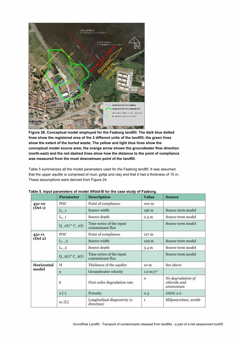
GrundRisk Landfill - Transport of contaminants released from landfills - a part of a risk assessment tool55
Figure 28. Conceptual model employed for the Faaborg landfill. The dark blue dotted lines show the registered area of the 2 different units of the landfill; the green lines show the extent of the buried waste; The yellow and light blue lines show the conceptual model source area; the orange arrow shows the groundwater flow direction (north-east) and the red dashed lines show how the distance to the point of compliance was measured from the most downstream point of the landfill. Table 5 summarizes all the model parameters used for the Faaborg landfill. It was assumed that the upper aquifer is comprised of mud, gyttja and clay and that it had a thickness of 10 m. These assumptions were derived from Figure 24.
Table 5. Input parameters of model Affald-B for the case study of Faaborg. Parameter Description Value Source
431-10 (Del 1)
POC Point of compliance 100 m
Ly_1 Source width 156 m Source term model
Lz_1 Source depth 2.4 m Source term model
Q_1(t) * C_1(t) Time series of the input contaminant flux
Source term model
431-11 (Del 2)
POC Point of compliance 127 m
Ly _2 Source width 109 m Source term model
Lz_2 Source depth 3.4 m Source term model
Q_2(t)* C_2(t) Time series of the input contaminant flux
Source term model
Horizontal model
H Thickness of the aquifer 10 m See above
u Groundwater velocity 1.0 m/y*
k First order degradation rate 0 No degradation of
chloride and ammonium
n [-] Porosity 0.3 JAGG 2.0
αL [L] Longitudinal dispersivity (x direction)
1 Miljøstyrelsen, 2016b

56 GrundRisk Landfill - Transport of contaminants released from landfills - a part of a risk assessment tool
αT [L] Transversal dispersivity (y direction)
0.01 Miljøstyrelsen, 2016b
αV [L] Vertical dispersivity (z direction)
0.005 Miljøstyrelsen, 2016b
R Retardation chloride 1
Retardation ammonium 5**
* The groundwater velocity of the upper aquifer was estimated assuming a 9‰ hydraulic gradient, 0.3 in porosity and 1·10-6 m/s a hydraulic conductivity of the aquifer which is made of mud, gyttja and clay (such low velocity was discussed above). ** The retardation factor for ammonium was chosen from literature (Christensen et al., 2001) assuming that ammonium retardation can be described as a sorption process (Ammonium is undergoing cation exchange, which is a non-linear process). Ammonium can also be transformed to nitrate or other nitrogen species in the aquifer. This is not included, but the worst case concentrations of nitrate (from ammonium) can be estimated from a stoichiometric conversion of ammonium to nitrate. 1 mol of ammonium is assumed to be converted to 1 mol nitrate or 1 mg/L of ammonium will be converted to 3,44 mg/l of nitrate.
3.2.4 Results for Faaborg Landfill. Model Affald-B This section shows the model results obtained from the two different units of Faaborg Landfill. Only chloride and ammonium will be shown in this example. Each unit has a different distance to the point of compliance; the input water discharge; input concentrations; geometry and spatial distribution are described above. Overall, the contaminant transport processes in the aquifer resulting from Faaborg Landfill might be too complex for such a simple contaminant transport model. The main assumptions of the model do not hold for this case:
- The model assumes that the groundwater velocity is not affected by the somewhat limited water discharge coming from the landfill. However, in this case the groundwater velocity was estimated to be very small (1 m/y) and the leachate velocity from the units vary over time from 155 m/y to 10 m/y. - The model was developed and tested for groundwater velocities in the same order of magnitude as the leachate velocities; however in this case the water discharging from the landfill has a velocity that is is up to 155 times higher.
The reason that the horizontal water discharge/ leachate velocities are very high compared to the groundwater velocity is likely due to the assumption of a no-flow boundary at the bottom of the landfill in the water balance calculation of the landfill units. It might be more correct to consider a scenario with vertical transport in the gyttja, mud and clay layer from the bottom of the landfill to the top of the deeper aquifer. Such scenario would apply model Affald-A to Faaborg Landfill and water balance calculations in the landfill that assume vertical water discharge from the bottom of the landfill (and not horizontal water discharge from the downstream submerged side of the landfill). Contaminant water concentrations According to our model assumptions, the concentrations in the aquifer resulting from unit 1 and 2 do not sum up with each other because their plumes do not overlap in the groundwater flow direction (see Figure 11). Therefore, the model computes the concentrations in the aquifer resulting both from unit 1 and unit 2 and then the results with the highest maximum concentrations are selected. Figure 29 shows the simulation results obtained using the model Affald-B applied to Faaborg Landfill. The simulation results only show the results from Unit 1 since it provides the highest

GrundRisk Landfill - Transport of contaminants released from landfills - a part of a risk assessment tool57
simulated maximum concentrations in the aquifer. The results show a significant difference between the 1D and the 3D model because of the different model assumptions, i.e. the 1D model assumes uniformly mixed concentration over the depth of the aquifer (deep and high flow rate aquifers will procuce low concentrations), whereas the 3D model assumes an infinitely deep aquifer. In this case the 1D model results in the highest concentrations due to the combination of a small aquifer discharge (that comes from the small input groundwater velocity of 1 m/y) and a limited aquifer thickness (10 m). Instead, the 3D model is not limited by the 10 m thick aquifer and can spread the contaminant plume to a larger depth (which is somehow unrealistic). Furthermore, the 3D model includes dispersion that in this case can be significant due to the combined effect of a large travel time to the POC and a significant decline of input concentrations over time. The concentrations from the 1D model are calculated from the mass discharge and so the concentration distributions have a similar pattern compared to the mass discharge patterns shown in Figure 30. The ammonium concentration resulting from the 1D model show a peak at the year 2440, i.e. 500 years after the beginning of the simulation time. This occurs because the inputs of groundwater velocity (1 m/y), retardation factor (5.0) and distance to the point of compliance (100 m) result in a 500 year travel time to the POC. On the other hands the chloride concentration resulting from the 1D model show a peak at the year 2040, i.e. 100 years after the beginning of the simulation time. This is because the retardation factor of chloride is 1.0 (chloride moves with the same velocity as groundwater and 5 times faster than ammonium). The concentrations resulting from the 3D model start raising some years earlier compared to the 1D model results because the 3D model include the processes of dispersion. In this case the results from the 1D model are employed since the maximum concentrations in the aquifer given by the 1D solution are higher than the 3D solution. The maximum concentrations from the 1D model are the same as the input maximum concentration and this is due to the limited flow in the aquifer combined with the limited aquifer thickness (not enough to dilute the mass discharge from the source) and also because the selected compounds do not degrade.
Figure 29. Concentration as a function of time. Simulation results for chloride and ammonium from the Faaborg landfill (model Affald-B). The results show only the concentrations resulting from Unit 1 because the concentrations resulting from Unit 2 are smaller and the plume of Unit 2 does not sum up with the plume of Unit 1 because
0
25
50
75
100
125
150
175
1940 2040 2140 2240 2340 2440
conc
entr
atio
n [m
g/L]
years
Ammoniumat the source
in the aquifer (3D model)
in the aquifer (1D fullymixed model)
0
100
200
300
400
500
600
1940 2040 2140 2240 2340 2440
conc
entr
atio
n [m
g/L]
years
Chloride

58 GrundRisk Landfill - Transport of contaminants released from landfills - a part of a risk assessment tool
they do not overlap in the groundwater direction. The concentrations in the aquifer are average concentrations over a 2 m long well screen.
Contaminant mass discharge The contaminant mass discharge at the Point of Compliance (POC) is defined as the mass discharge over an infinite plane perpendicular to the groundwater flow direction and located at the POC distance. Therefore, the total mass discharge from the landfill is the superposition of the contribution from each of the 2 different units of Faaborg Landfill. Figure 30 shows the simulation results obtained using the model Affald-B applied to Faaborg Landfill. The simulation results show both the single contributions from each unit and the total breakthrough curve. The maximum mass discharge from each unit occurs at different times because of different transport times due to both different horizontal transport distances and different periods of the input leachate time series. The simulated ammonium mass discharge of Figure 30 is not fully visible within the 500 years simulation time. This is due to the inputs of groundwater velocity (1 m/y), retardation factor (5.0) and distance to the point of compliance (100 m) that make the travel time to the POC to be exactly 500 years for Unit 1 and > 500 years for Unit 2 because Unit 2 is located at 127 m distance to the POC. The maximum mass discharge in this case can be overestimated because the 1D model does not include dispersion. Dispersion can have an impact in this case due to the combined effect of a large travel time to the POC and the steep decline of input concentrations over time
Figure 30. Contaminant mass discharge in the aquifer as a function of time (the mass discharge of ammonium in unit 2 is zero as it starts rising after the 500-year simulation period). Simulation results for chloride and ammonium from Faaborg landfill (model Affald-B). The results show both the total mass discharge resulting from the superposition of unit 1 and 2 and the single unit mass discharge.
0
500
1000
1500
2000
2500
3000
1940 2040 2140 2240 2340 2440
mas
s dis
char
ge [
kg/y
]
years
Ammonim
Unit 1
Unit 2
Unit 1 + Unit 2
0
2000
4000
6000
8000
10000
12000
2009 2059 2109
mas
s dis
char
ge [
kg/y
]
years
Chloride

GrundRisk Landfill - Transport of contaminants released from landfills - a part of a risk assessment tool59
3.2.5 Conclusion of the model Affald-B application to the landfill of Faaborg
The results of the model Affald-B application to the landfill of Faaborg showed the following:
- The concentrations from the two different units of the landfill do not sum up in the aquifer since the units do not overlap in the groundwater flow direction. - The maximum concentrations of chloride and ammonium in the aquifer equal the maximum input concentrations. This is because these compounds do not degrade and also because the small groundwater flow velocity combined with the small aquifer thickness do not provide enough groundwater flux to dilute the mass discharge from the source. - The maximum ammonium concentrations in the aquifer occur after 500 year of simulation. This is due to the combination of a small groundwater velocity and retardation factor. - The total mass discharge of ammonium occurs mostly after the 500-year simulation period. - The total mass discharge of chloride from the landfill (within the 500-year period) is the sum of the single units’ contributions. The contribution from each unit occurs at different periods of time mainly due to the different transport distances to the POC. Add conclusions for metals and degradable organics. - Nickel was not shown in the plot because of the high retardation factor which would delay breakthrough beyond the 500-year simulation time mainly due to the large transport time resulting from the very low groundwater velocity. - Benzene was not shown in the following examples as the resulting concentrations at the POC would be too low to be reported and discussed.
60 GrundRisk Landfill - Transport of contaminants released from landfills - a part of a risk assessment tool
3.3 Hørløkke Landfill. Application of the model ‘Affald-A’ The landfill of Hørløkke is located in the town of Vojens. In the period 1968 to 1971 it received mainly construction material and municipal waste from Vojens city. Additionally, it also received sludge from Vojen's waste water treatment plant for a period of time. From 1972, when the Arnitlund landfill site opened, Hørløkke's was functioning as a dump site without supervision. During the period 1975 to 1978 there was only limited activity at the site. The last areas that were used before the coverage in 1978 were (according to aerial photographs) the northeast and northwestern corners. The landfill was covered with clay and sandy clay (in Danish: klæg) (Sønderjyllands Amt, 2003). Investigations carried out in the year 2000 showed that in the northeastern part of the landfill site, among other things, there were deposited asphalt residues and building waste and there was no household waste. Moreover, some oil waste was found. According to the municipality of Vojens, the landfill was levelled (in Danish: planeret) and vegetation planted in October 1984. The first soil and groundwater investigations began in 1985 by the former County of Sønderjylland. 3.3.1 Geology and hydrogeology Figure 31 shows a conceptual geological cross section of the area around the landfill of Hørløkke (Wernberg et al., 2012). The figure also shows the location of the landfill, the groundwater level and flow direction and the contaminant plume. The figure shows that there is a large unconfined aquifer and that the landfill lies just above the top of the aquifer. The aquifer consists of sand and the bottom of the aquifer lies approximately 80 m below terrain level (Wernberg et al., 2012). Region Syddanmark (2009) reported several groundwater equipotential maps using head measurements measured between 2006 and 2009. Overall, the groundwater flow direction is stable throughout the observed period and the groundwater flow direction is directed towards west (Figure 32). Groundwater gradients in the area were estimated to be 4-5 ‰ (Region Syddanmark, 2009) and 6.5 ‰ (Højberg et al., 2015). Vertical downward groundwater head gradients were also observed. The calibrated hydraulic conductivity of the sand is 1.5·10-4 m/s. The groundwater recharge in the area was estimated to be 351 mm/y (Wernberg et al., 2012); 533 mm/y (JAGG 2.0) and 438 mm/y (Højberg et al., 2015).

GrundRisk Landfill - Transport of contaminants released from landfills - a part of a risk assessment tool61
Figure 31. Conceptual geological cross section. flow direction and contaminant plume at Hørløkke Landfill (note the different horizontal and vertical scale of the figure). Wernberg et al. (2012).
3.3.2 Description of the landfill source The input concentration and water discharge from the different compartments of the landfill were provided by the Source term model. The time period of the input concentration time series is 500 years. The geometry of the source area is assumed to be rectangular and the source length and height were provided by the Source term model. Benzene, iron (dissolved),and nickel were selected as “model compounds” as they are present in high to moderate concentrations, represent two source functions (leaching curves) and their horizontal transport will be different, because of different retardation factors. 3.3.3 Conceptual model and parameters The model Affald-A was chosen because the bottom of the landfill is located above the aquifer. Vertical transport from the bottom of the landfill to the top of the groundwater table was not simulated since the bottom of the landfill lies immediately above the top of the groundwater table. Figure 32 shows the conceptual model (geometry and location of the landfill) used to simulate the landfill of Hørløkke; these data were provided by the Source term model. Figure 32also shows the groundwater flow direction and the Point of Compliance (POC) assumed to be 100 m downstream the most downstream point of the landfill.
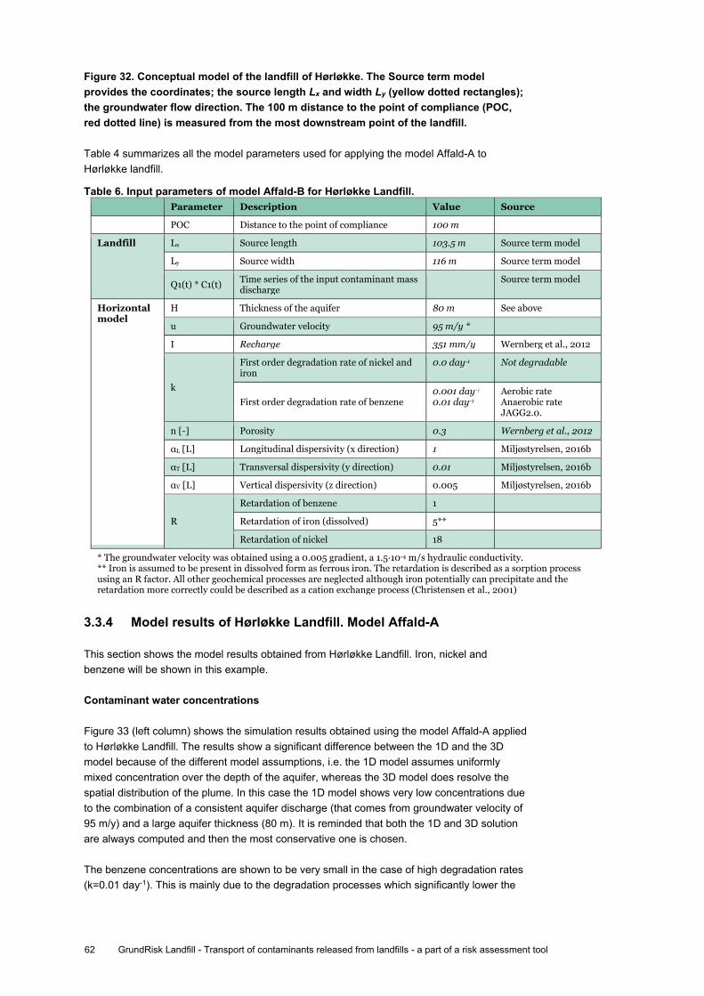
62 GrundRisk Landfill - Transport of contaminants released from landfills - a part of a risk assessment tool
Figure 32. Conceptual model of the landfill of Hørløkke. The Source term model provides the coordinates; the source length Lx and width Ly (yellow dotted rectangles); the groundwater flow direction. The 100 m distance to the point of compliance (POC, red dotted line) is measured from the most downstream point of the landfill. Table 4 summarizes all the model parameters used for applying the model Affald-A to Hørløkke landfill.
Table 6. Input parameters of model Affald-B for Hørløkke Landfill. Parameter Description Value Source
POC Distance to the point of compliance 100 m
Landfill Lx Source length 103.5 m Source term model
Ly Source width 116 m Source term model
Q1(t) * C1(t) Time series of the input contaminant mass discharge
Source term model
Horizontal model
H Thickness of the aquifer 80 m See above
u Groundwater velocity 95 m/y *
I Recharge 351 mm/y Wernberg et al., 2012
k
First order degradation rate of nickel and iron
0.0 day-1 Not degradable
First order degradation rate of benzene 0.001 day-1
0.01 day-1 Aerobic rate Anaerobic rate JAGG2.0.
n [-] Porosity 0.3 Wernberg et al., 2012
αL [L] Longitudinal dispersivity (x direction) 1 Miljøstyrelsen, 2016b
αT [L] Transversal dispersivity (y direction) 0.01 Miljøstyrelsen, 2016b
αV [L] Vertical dispersivity (z direction) 0.005 Miljøstyrelsen, 2016b
R
Retardation of benzene 1
Retardation of iron (dissolved) 5**
Retardation of nickel 18
* The groundwater velocity was obtained using a 0.005 gradient, a 1.5·10-4 m/s hydraulic conductivity. ** Iron is assumed to be present in dissolved form as ferrous iron. The retardation is described as a sorption process using an R factor. All other geochemical processes are neglected although iron potentially can precipitate and the retardation more correctly could be described as a cation exchange process (Christensen et al., 2001)
3.3.4 Model results of Hørløkke Landfill. Model Affald-A This section shows the model results obtained from Hørløkke Landfill. Iron, nickel and benzene will be shown in this example. Contaminant water concentrations Figure 33 (left column) shows the simulation results obtained using the model Affald-A applied to Hørløkke Landfill. The results show a significant difference between the 1D and the 3D model because of the different model assumptions, i.e. the 1D model assumes uniformly mixed concentration over the depth of the aquifer, whereas the 3D model does resolve the spatial distribution of the plume. In this case the 1D model shows very low concentrations due to the combination of a consistent aquifer discharge (that comes from groundwater velocity of 95 m/y) and a large aquifer thickness (80 m). It is reminded that both the 1D and 3D solution are always computed and then the most conservative one is chosen. The benzene concentrations are shown to be very small in the case of high degradation rates (k=0.01 day-1). This is mainly due to the degradation processes which significantly lower the

GrundRisk Landfill - Transport of contaminants released from landfills - a part of a risk assessment tool63
concentration downstream the landfill. The maximum concentrations of benzene in the case of low degradation rates (k=0.001 day-1) are approximately a third of the maximum input concentrations. The peak concentration occurs only a couple of years later than in the source due to the high groundwater velocity and no retardation processes. The degradation will be dependent on the actual redox conditions down-gradient landfill. It is expected that the core of the plume will be anaerobic closest to the landfill. The iron and nickel concentrations resulting from the 3D model show both a reduction and a time delay of the maximum input concentrations. The maximum nickel concentrations in the aquifer are approx. 70% lower than the maximum input concentrations and the maximum concentrations of iron are approx. 50% lower. These reductions are due to both (1) the dispersion of the contaminant plume and (2) the sorption processes. Dispersion can play an important role in this case since the input concentration shows significant variation in time. More sorption in this case also contribute to reduce the maximum concentrations. This can be observed in the simulated concentrations of nickel and iron. Nickel has a higher retardation factor which makes the nickel plume velocity slower compared to the plume velocity of iron. A lower plume velocity makes the contaminant concentrations at the point of compliance spreading over a larger time period ‘smoothening’ the peak concentration. It should also be noted that the model neglects other geochemical processes, which means that iron stays in solution as ferrous iron assuming anaerobic conditions in the aquifer. If a shift to aerobic conditions appears, dissolved iron will rapidly precipitate and not be further transported. Mobility of nickel can be enhanced by interaction with organic matter, which already was adressed by using a low Kd value (R factor) for nickel in the lower range of observed Kd-values.

64 GrundRisk Landfill - Transport of contaminants released from landfills - a part of a risk assessment tool
Figure 33. Simulated concentration and contaminant mass discharge as a function of time. The concentrations in the aquifer are average concentrations over a 2 m long well screen. Note that the concentration are given either in μg/L oR mg/L
Contaminant mass discharge Figure 33 (right column) shows the simulation results obtained using the model Affald-A applied to Hørløkke landfill. The contaminant mass discharge at a the Point of Compliance (POC) is defined as the mass discharge over an infinite plane perpendicular to the groundwater flow direction and located at the POC distance.
0
2
4
6
8
10
1976 2001 2026 2051 2076
conc
entr
atio
n [μ
g/L]
years
Benzene (k=0.01 day-1)
in the aquifer(1D model)in the aquifer(3D modelat the source
0
0.01
0.02
0.03
0.04
0.05
1976 2001 2026 2051 2076
mas
s dis
char
ge [k
g/y]
years
Benzene (k=0.01 day-1)
in the aquiferat the source
0
20
40
60
80
1976 2001 2026 2051 2076
conc
entr
atio
n [μ
g/L]
years
Nickel
0
0.1
0.2
0.3
0.4
0.5
1976 2001 2026 2051 2076
mas
s dis
char
ge [k
g/y]
years
Nickel
0
10
20
30
40
50
1976 2001 2026 2051 2076
conc
entr
atio
n [m
g/L]
years
Iron
0
50
100
150
200
250
1976 2001 2026 2051 2076
mas
s dis
char
ge [k
g/y]
years
Iron
0
2
4
6
8
10
1976 2001 2026 2051 2076
conc
entr
atio
n [μ
g/L]
years
Benzene (k=0.001 day-1)
0
0.01
0.02
0.03
0.04
0.05
1976 2001 2026 2051 2076
mas
s dis
char
ge [k
g/y]
years
Benzene (k=0.001 day-1)

GrundRisk Landfill - Transport of contaminants released from landfills - a part of a risk assessment tool65
The contaminant mass discharge of benzene is smaller compared to the input mass discharge. This is mainly due to the degradation processes which lower the mass discharge downstream the landfill. The accumulated mass discharge of nickel and iron (the area below the mass discharge time series) is the same as the accumulated input mass discharge because these compounds do not degrade. The mass discharge of nickel shows a larger time delay due to the higher sorption properties compared to iron. Moreover, the peak mass discharge of nickel shows a larger reduction of maximum concentration compared to iron. This is mainly due to the lower contaminant plume velocity of nickel which makes the mass discharge at the point of compliance spreading over a larger time period ‘smoothening’ the peak mass discharge. The maximum mass discharge in this case can be overestimated because the 1D model does not include dispersion. Dispersion in this case can have a significant impact due to a significant decline of input concentrations over time 3.3.5 Conclusion of the model Affald-A application to the landfill of
Hørløkke The results of the model Affald-A application to the landfill of Hørløkke showed the following:
- The maximum concentrations in the aquifer are found by the 3D model. This means that the aquifer is assumed to be thick. - The maximum concentrations and contaminant mass discharge of benzene in the aquifer are reduced due to degradation. Degradation rates significantly influence the outputs concentrations and mass discharge. - The maximum concentrations of nickel and iron with 70% and 50% respectively mainly due to dispersion. - The contaminant mass discharge of iron and nickel in the aquifer is the same as the total input mass discharge as these compounds do not degrade. - The maximum contaminant discharge per year of iron and nickel in the aquifer is reduced by up to 50%.
66 GrundRisk Landfill - Transport of contaminants released from landfills - a part of a risk assessment tool
4. Practical considerations
The model GrundRISK Landfill includes two separate models Affald-A and Affald-B developed in this work. GrundRISK Landfill is a set of contaminant transport models to be applied as a part of a site specific risk assessment tool for landfills. GrundRISK Landfill aims to provide a first assessment of transport of contaminants in soil and groundwater based on generally scarce data. As such it is designed to be fairly simple (as few parameters as possible), to run fast (maximum few minutes) and to be adaptable to the very different hydrogeological conditions that can be found at Danish landfills. This means that the user of the model must be aware of the main model assumptions and the required landfill and aquifer property parameters. The results from the models will be mathematically correct and in most cases conservative, but they will not always reflect the actual conditions or include all relevant processes. Therefore, the user needs to reflect on the outputs from the model and in particular consider if basic assumptions are violated in the setup of the model. In the following we summarize some common situations that can occur when using the models. Model-A: - The concentration breakthrough curve at the POC resulting from the 3D model can show a
flat peak (i.e. see the chloride concentrations in the case study of Tandskov of Figure 19). This flat peak is the result of the model cutting off all the concentrations (calculated with the analytical solution) that are higher than the maximum input concentration. This happens because the 3D analytical solution can give higher concentration than the maximum input concentration because it does not account for the additional water added through the source and therefore does not account for both the dilution due to the extra water and the vertical advection that occurs below the source area. Basically this means that source concentration will not be diluted in the aquifer because of the size of the landfill and large amount of leachate generated compared to the flow in the aquifer.
Model-B: - The vertical flow velocity through the source is very different compared to the horizontal
groundwater velocity (e.g. the vertical velocity from the landfill was up to 155 times higher than the groundwater velocity in the case study of Faaborg). The vertical flow velocity and groundwater velocity can be considered acceptable/reasonable only if they are in the same order of magnitude; otherwise the assumption that the groundwater velocity is not affected by the water flow through the source is no longer valid. In such cases the user should either reconsider the water balance of the landfill (in the Source term model) in order to have a more reasonable match between source velocity and groundwater velocity or assume that the water discharge/ leachate from the landfill is from the bottom of the landfill (in the Source term model), therefore using the transport model Affald-A. If the velocities still seem to be very different, the basic assumptions of model B are violated, and the use of a more advanced numerical model could be considered.
Model-A and Model-B: - The concentration breakthrough curve at the POC resulting from the 1D model shows a flat
peak (i.e. see the chloride concentrations in the case study of Faaborg landfill of Figure 29). This flat peak is the result of the model cutting off all the concentrations (calculated with the analytical solution) that are higher than the maximum input concentration. The concentrations are cutoff because the 1D analytical solution does not account for the additional water added through the source. Overall, this means that the groundwater flux (for

GrundRisk Landfill - Transport of contaminants released from landfills - a part of a risk assessment tool67
instance the annual groundwater flux) is not large enough to dilute the contaminant mass. This can generally happen with small aquifer depth and/or small groundwater velocities.
- The 1D model outputs higher concentrations than the 3D model (i.e. see the chloride concentrations in the case study of Faaborg of Figure 29). This can be due to (1) the combined effect of a small aquifer depth and/or a small groundwater velocity or (2) the fact that the 1D model does not include dispersion. In this case the user should carefully consider the case-specific processes involved (i.e. if the input source concentrations were constant in time then dispersion would not have an impact on the maximum concentrations) in order to better judge the model outputs. Moreover, the user can also compare the concentrations obtained with the 1D and 3D model with the uncertainty of the input source concentrations.
Overall, the dispersion and dilution processes are likely to produce a somewhat limited reduction of the maximum source concentrations at distances up to few hundred meters downstream landfills due to the combination of the large areas of landfills, the limited distance downstream landfills and the large contaminant mass discharge from landfills. Finally the models are intended to provide conservative results, which in some cases compromise attenuation processes. If the user finds the results are too conservative the solution is to scrutinize the assumptions, and parameters. This may lead to the conclusion that the models are not able to simulate the actual conditions or biogeochemical processes properly. The next step might be to apply a more advanced reactive solute transport model (numerical model). Our application of the models at three landfill sites, however, indicates that the current data for Danish landfills will be scarce and maybe the biggest limitation for more detailed risk assessment. The main data limitations and challenges are related to three types of gaps in information and parameters:
- The source term and its temporal development in a 500 year timescale is in general critical for the results, and the scarce data and heterogeneity for old landfills in particular will be a major issue. However, even for controlled landfills several assumptions have to be made about the physical conditions, water balances (flows), and compounds. This is discussed in detail in the Miljøstyrelsen (2018a,b).
- The two models developed in this report require data outside the landfilled area about hydrogeology properties and groundwater systems in order to simulate the transport downstream. This has not been the focus for current data collection and investigations at controlled landfills and the data is scarce. For old landfills the data is typically stronger for the surroundings than for the landfill itself. In both cases the conditions may have changed (e.g. groundwater abstraction, change in land use) or will change over the simulation period as demonstrated in the examples in this report.
- A reactive solute transport model (numerical) has to be populated with appropriate parameters for the additional reactive processes included e.g. non-linear sorption, cation exchange processes, dissolution/precipitation of minerals and sequential degradation of organic contaminants or nutrients (ammonium). This requires estimations and/or measurements of parameters such as Freundlich sorption parameters, cation exchange capacity, selectivity cofficients, and degradation/nitrification rates, which is believed to be a major effort and an unrealistic task in some cases.
We expect because of these challenges that applications of more advanced reactive solute transport models will be constrained with lack of data. Thus more advanced models are likely not to produce more correct results with the currently available data. We therefore also suggest that there should be more focus on closing the data gaps instead of demanding application of more advanced reactive transport models in order to improve risk assessment of

68 GrundRisk Landfill - Transport of contaminants released from landfills - a part of a risk assessment tool
groundwater resources from landfills. This is in particular relevant for active, controlled landfill sites, where additional monitoring of water balances and compounds still is possible.

GrundRisk Landfill - Transport of contaminants released from landfills - a part of a risk assessment tool69
5. References
Århus Amt, 2003: Affaldscenter Tandskov. Kontrol af grundvandskvaliteten ved lossepladsen og kontrol af recipient Resdal Bæk
Århus Amt, 2006. Statusrapport Affaldscenter Tandskov. Aarhus Amt. Natur og Miljø. Appelo, C.A.J., and Postma, D., 1993, Geochemistry, groundwater and pollution: Rotterdam,
A.A. Balkema, 536 p. Carl Bro 2007. Silkeborg Kommune. Affaldscenter Tandskov. Overgangsplan. Projekt:
30.4608.02. Christensen, T.H., Kjeldsen, P., Bjerg, P.L., Jensen, D.L., Christensen, J.B., Baun, A.,
Albrechtsen, H.-J. & Heron, G., 2001. Biogeochemistry of landfill leachate plumes. Applied Geochemistry, 16, 659-718.
Fischer et al., 1979. Mixing in inland and coastal waters. ISBN-13: 978-0122581502 Højberg et al., 2015. DK-model 2014 - Model opdatering og kalibrering. GEUS rapport 2015/8,
København JAGG 2.0. http://mst.dk/virksomhed-myndighed/jord/it-vaerktoejer-til-vurdering-af-jord/ Miljøstyrelsen, 1998. Oprydning på forurenede lokaliteter, hovedbind og appendiks. Vejledning
fra Miljøstyrelsen nr. 6 og 7, 1998. Miljøstyrelsen, 2013. Manual for program til risikovurdering – JAGG 2.0. Miljøprojekt nr. 1508,
2013. Miljøstyrelsen, 2016a. JAGG 2 - Vertikal transport ned til førstkommende betydende magasin.
Miljøprojekt nr. 1828, 2016. Miljøstyrelsen, 2016b. GrundRisk. Beregningsmodel til risikovurdering af grundvandstruende
forureninger. Miljøprojekt nr. 1865, 2016. Miljøstyrelsen, 2017. GrundRisk. Coupling of vertical and horizontal transport models.
Miljøprojekt nr. 1915, 2017. Miljøstyrelsen (2018a). Udvikling af metodik til risikovurdering ved deponering af affald –
Kildestyrke fase 1 - konceptuelle modeller. Miljøprojekt nr. 2057, 2018. Miljøstyrelsen (2018b). Udvikling af metodik til risikovurdering ved deponering af affald –
Kildestyrke fase 2 - Opbygning af kildestyrkemodel. Miljøprojekt nr. 2058, 2018. Naturforvaltningsprojekt, 1993, Fyns Amt. Sundet ved Fåborg. Nielsen, S., Vestervang, S., Nilausen, L., and von Huth, A., 1994. Forureningsundersøgelse af
lossepladserne reg.nr. 431-10 og 431-11 samt del af Sundstien, Faaborg. Technical report, COWIconsult, Lyngby, Denmark. In collaboration with Fyns Amt.
Region Syddanmark, 2009. Forureningsundersøgelser ved Hørløkke. Statusrapport, 2007-2009. Foreløbig. Alectia.
Sønderjyllands Amt, 2003. Forureningsundersøgelser ved Hørløkke Landfill. Statusnotat, Februar 2003.
Troldborg, M., Binning, P.J., Nielsen, S., Kjeldsen, P., Christensen, A.G., 2009. Unsaturated zone leaching models for assessing risk to groundwater of contaminated sites. Journal of hydrology. Volume 105, Issues 1–2.
Wernberg, T, Hansen, T.B., Pedersen, J.K., Christensen, J.F., Johnsen, R., Jensen, T.W., 2012. Assessing the impact of climate change on two landfill sites using large scale models - Preparing future management of the two sites. Draft paper.
Wexler, E.L., 1992. Analytical Solutions for one-, two- and three-dimensional solute transport in ground-water systems with uniform flow. Chapter B7 in Techniques of Water-Resources Investigations of the United States Geological Survey. Book 3 Applications of

70 GrundRisk Landfill - Transport of contaminants released from landfills - a part of a risk assessment tool
Hydraulics. U.S. Department of the interior. U.S. Geological Survey. United States Government Printing Office, 1992.
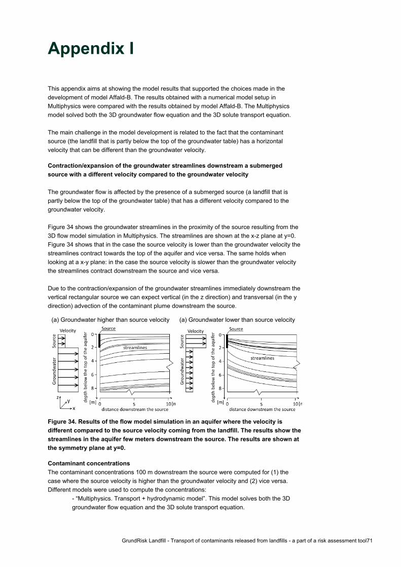
GrundRisk Landfill - Transport of contaminants released from landfills - a part of a risk assessment tool71
Appendix I
This appendix aims at showing the model results that supported the choices made in the development of model Affald-B. The results obtained with a numerical model setup in Multiphysics were compared with the results obtained by model Affald-B. The Multiphysics model solved both the 3D groundwater flow equation and the 3D solute transport equation. The main challenge in the model development is related to the fact that the contaminant source (the landfill that is partly below the top of the groundwater table) has a horizontal velocity that can be different than the groundwater velocity. Contraction/expansion of the groundwater streamlines downstream a submerged source with a different velocity compared to the groundwater velocity The groundwater flow is affected by the presence of a submerged source (a landfill that is partly below the top of the groundwater table) that has a different velocity compared to the groundwater velocity. Figure 34 shows the groundwater streamlines in the proximity of the source resulting from the 3D flow model simulation in Multiphysics. The streamlines are shown at the x-z plane at y=0. Figure 34 shows that in the case the source velocity is lower than the groundwater velocity the streamlines contract towards the top of the aquifer and vice versa. The same holds when looking at a x-y plane: in the case the source velocity is slower than the groundwater velocity the streamlines contract downstream the source and vice versa. Due to the contraction/expansion of the groundwater streamlines immediately downstream the vertical rectangular source we can expect vertical (in the z direction) and transversal (in the y direction) advection of the contaminant plume downstream the source.
(a) Groundwater higher than source velocity
(a) Groundwater lower than source velocity
Figure 34. Results of the flow model simulation in an aquifer where the velocity is different compared to the source velocity coming from the landfill. The results show the streamlines in the aquifer few meters downstream the source. The results are shown at the symmetry plane at y=0.
Contaminant concentrations The contaminant concentrations 100 m downstream the source were computed for (1) the case where the source velocity is higher than the groundwater velocity and (2) vice versa. Different models were used to compute the concentrations:
- “Multiphysics. Transport + hydrodynamic model”. This model solves both the 3D groundwater flow equation and the 3D solute transport equation.

72 GrundRisk Landfill - Transport of contaminants released from landfills - a part of a risk assessment tool
- “Scenario with hydrodynamics”. This model uses the analytical solution of the 3D transport equation (which was developed for a uniform horizontal groundwater flow field and a fixed concentration input boundary) and also it contracts/expands the size of the source in order to simulate the contraction/expansion of the groundwater streamlines immediately downstream the source as explained above. This is the model approach that was used in the model Affald-B and the correction of the source dimension Lz*Ly was explained in Section 2.3.2. The new larger/smaller source size has the right mass discharge and expands/shrinks the area with the source input concentration. - “Scenario without hydrodynamics”. This model uses the analytical solution of the 3D transport equation (which was developed for a uniform horizontal groundwater flow field and a fixed concentration input boundary) and keep the original source size Lz and Ly and the input source concentraion. In this way the model has the wrong input mass discharge (and the right source concentration) since the concentration is multiplied by the lower/higher groundwater velocity compared to the source velocity. - “Scenario mass discharge boundary condition”. This model uses the analytical solution of the 3D transport equation (which was developed for a uniform horizontal groundwater flow field and a fixed concentration input boundary) and keep the original source size Lz and Ly. The source concentration is modified in order to have the right contaminant mass discharge at the source. The source concentration is modified based on the ratio between the groundwater velocity and the source velocity, i.e. if the groundwater velocity is 10 m/y and the source velocity is 20 m/y then the input concentration is multiplied by 2 so that the mass discharge through the Lz*Ly source is correct. In this way the model has the wrong input source concentrations but the right mass discharge.
Figure 35 shows the simulations results. The following observations can be made:
- “Scenario with hydrodynamics” is the one that best reproduces the results obtained by the Multiphysics model in both the cases where the groundwater velocity is smaller and larger than the source velocity. - “Scenario without hydrodynamics” can underestimate the concentrations in the case the source velocity is larger than the groundwater velocity. In the case the groundwater velocity is lower than the source velocity, the contaminant mass discharge is also smaller and thus concentrations in the aquifer are underestimated. - “Scenario mass discharge boundary condition” underestimates the concentrations in the case the source velocity is smaller than the groundwater velocity. In the case the groundwater velocity is larger than the source velocity, the concentrations over the source area Ly*Lz are reduced in order to adjust the correct contaminant mass discharge at the source area Ly*Lz and thus concentrations in the aquifer are underestimated.

GrundRisk Landfill - Transport of contaminants released from landfills - a part of a risk assessment tool73
Figure 35. Comparison of different scenarios (different model approaches) with the results obtained with a Mulitiphysics numerical model that included both the 3D groundwater flow equation and the 3D solute transport equation.
Based on the observations above, the model approach of model Affald-B was considered to be the most suitable.
-10
-8
-6
-4
-2
0
0.0 2.0 4.0 6.0 8.0 10.0
dept
h be
low
the
top
of th
e aq
uife
r [m
]
concentration [mg/L]
Groundwater vel. = 20 m/y; source vel. = 6.7 m/y
Multiphysic. Tansport + hydrodynamic model
Co
scenario with hydrodynamics
scenario without hydrodynamics
scenario mass discharge boundary condition
-10
-8
-6
-4
-2
0
0.0 5.0 10.0 15.0 20.0 25.0 30.0
dept
h be
low
the
top
of th
e aq
uife
r [m
]
concentration [mg/L]
Groundwater vel. = 20 m/y; source vel. = 60 m/y

74 GrundRisk Landfill - Transport of contaminants released from landfills - a part of a risk assessment tool
Appendix II
This appendix shows the comparison of the simulated concentrations obtained from Affald-A and from a numerical model setup in Multiphysics. The Multiphysics model solved both the 3D groundwater flow equation and the 3D solute transport equation. The unit 1 of Tandskov Affaldscenter (model parameters are reported in the relative case study shown in the report) is used for the comparison. The main challenge in the application of model Affald-A is related to the fact that the model assumes (1) that the velocity in the aquifer is uniform and horizontal and (2) that the additional water discharge of the landfill is small so that it does not affect the water balance of the aquifer and it does not generate vertical velocities below the landfill area. Therefore, the model does not account for (1) the vertical downward groundwater velocities generated by the water discharge below the landfill area; (2) contaminant dilution due to the additional water discharge; (3) the variation of horizontal groundwater velocities in the flow direction (shown below). Overall, the model Affald-A gives 2.3 times higher maximum concentrations 100 m downstream Unit 1 of Tandskov Affaldscenter compared to the Multiphysics model. This overestimation is considered acceptable in the context of risk assessment. Groundwater velocity in the aquifer This section shows the groundwater velocity in the aquifer in the area of Tandskov considering only Unit 1. The Multiphysics model setup was used to solve the 3D groundwater flow equation. The model setup consists of a rectangular aquifer with no-flow boundary conditions at the bottom of the aquifer and water inflow at the top of the aquifer (water discharge below the landfill area and recharge over the rest of the area). Figure 36 shows the horizontal velocity in the flow direction of the aquifer (underneath the landfill area and in the surroundings). The horizontal velocity in the aquifer is uniform over the depth. The overall increase of horizontal velocity moving downstream in the aquifer is due to the continuous recharge/leachate over the top of the aquifer. The velocity gradient is higher in the landfill area as the water discharge is higher than the recharge in this case. The leachate flux is 0.37 m/y whereas the recharge is 0.11 m/y. The horizontal groundwater velocity downstream the landfill is approx. 116 m/y and this was matched in order to have the same velocity that is used in the application of model Affald-A to the case study of Tandskov. The vertical velocities at the top of the aquifer equal the input recharge/leachate velocities and they linearly decrease to zero at the bottom (no-flow boundary) of the aquifer.

GrundRisk Landfill - Transport of contaminants released from landfills - a part of a risk assessment tool75
Figure 36. Horizontal groundwater velocity in the aquifer. The zero horizontal distance corresponds to the model setup and was set to 100 m upstream the landfill in this case. The dotted lines show the area in the aquifer which lies underneath the simulated landfill unit. Concentrations in the aquifer Figure 37 shows the simulated concentrations as a function of time and depth at different distances downstream the landfill (100, 200 and 400 m downstream). The simulation was done for unit 1 of Tandskov Affaldcenter (see the case study above for the model parameters). The results show the following:
- Affald-A overestimated the maximum concentrations by a factor of 1.75-2.3 (1.75 times higher maximum concentrations 100m downstream and 2.3 times higher at 400m). The farther the distance downstream the landfill, the more the Affald-A solution approaches the Multiphysics solution. Nevertheless, it has to be considered that the larger the distance downstream the landfill, the larger is the groundwater velocity increase in the aquifer.
- The concentrations as a function of time from the 2 models follow similar patterns, even though the concentrations from Affald-A are higher.
- The concentrations as a function of the depth from the 2 models show different patterns. The concentration from Affald-A underestimates the depth of the center of the plume. This happens because the plume in Affald-A starts travelling downward only downstream the landfill whereas in the Multiphysics model the plume starts travelling downward below the landfill area that in this case is large (Lx = 381 m).
- The concentrations resulting from Affald-A often exceeds the maximum input concentration C0. This happens because the model do not account (1) for the water added at the source and (2) for the vertical velocities below the source.
Overall, the model Affald-A gives 2.3 times higher maximum concentrations 100 m downstream Unit 1 of Tandskov Affaldscenter compared to the Multiphysics model.
90
100
110
120
130
0 200 400 600 800 1000
horiz
onta
l vel
ocity
in th
e aq
uife
r [m
/y]
horizontal distance [m]
unit 1 of the landfill

76 GrundRisk Landfill - Transport of contaminants released from landfills - a part of a risk assessment tool
Figure 37. Simulated concentrations as a function of time and depth at (a) 100 m downstream the landfill; (b) 200 m downstream the landfill and (c) 400 m downstream the landfill. The concentrations were simulated using both a Multiphysics model with 3D flow and transport equations and the 3D solution of the model Affald-A. Unit 1 of Tandskov Affaldscenter was simulated.
[Tekst - Slet ikke efterfølgende linje, sektionsskifte]
0
1000
2000
3000
4000
5000
0 10 20 30 40
conc
entr
atio
n [m
g/L]
time [years]
(a) POC=100 m Multiphysics
Affald-A
maximum Co
0
1000
2000
3000
4000
5000
0 10 20 30 40
conc
entr
atio
n [m
g/L]
time [years]
(b) POC=200 m
0
1000
2000
3000
4000
5000
0 10 20 30 40
conc
entr
atio
n [m
g/L]
time [years]
(c) POC=400 m
-10
-8
-6
-4
-2
0
0 1000 2000 3000 4000 5000
dept
h be
low
the
top
of th
e aq
uife
r [m
]
concentration [mg/L]
-10
-8
-6
-4
-2
0
0 1000 2000 3000 4000 5000
dept
h be
low
the
top
of th
e aq
uife
r [m
]
concentration [mg/L]
-10
-8
-6
-4
-2
0
0 1000 2000 3000 4000 5000
dept
h be
low
the
top
of th
e aq
uife
r [m
]
concentration [mg/L]


The Danish Environmental Protection Agency Haraldsgade 53 DK-2100 København Ø www.mst.dk
GrundRisk Landfill The Danish Environmental Protection Agency has in collaboration with the Danish Waste Association and DepoNet, completed a project with the purpose of developing a methodology for visualizing the site-specific contamination of ground water, surface waters and nature surrounding Danish landfills. The methodology includes description of the contaminant source, transport of contaminants in and above the saturated zone as well as evaluation of the environmental impact. The GrundRisk model was developed by DTU and the Danish Environmental Protection Agency to assess the risk posed by contaminated sites to groundwater. This report presents the adaptation and application of the GrundRisk model for risk assessment of Danish landfills posing a threat to groundwater and surface water. The risk assessment tool for landfills is referred to as GrundRisk Landfill and consists of two models based on time-dependent analytical solutions. The models simulate the contaminant concentration as a function of time, through vertical and horizontal transport between the contaminant source and a point of compliance downstream in underlying groundwater. The model is given an input of contaminant fluxes (concentration of contaminants and amounts of leachate as a function of time) from landfills, as determined by a separate source term model. As a new application, GrundRisk Landfill is able to take into account all landfill units including older units without liners. GrundRisk Landfill keeps record of the time-dependent leaching of contaminants into the groundwater from the different units. This report presents the vertical and horizontal transport models and the assumptions made in the models.