guadalupe river watershed loading hspf model: year · pdf fileguadalupe river watershed...

Guadalupe River Watershed Loading HSPF Model:Year 3 final progress report

Prepared by

Michelle Lent and Lester McKeeSan Francisco Estuary Institute

Richmond, California

For

The Regional Monitoring Program for Water Quality in San Francisco Bay (RMP)Sources Pathways and Loading Workgroup (SPLWG)

Final DRAFTDecember, 2011

of 22 Guadalupe River loads HSPF model

This progress report can be cited as:Lent, M. and McKee, L., 2011. Guadalupe River Watershed Loading HSPF Model:Year 3 final report. A technical progress report prepared for the Regional MonitoringProgram for Water Quality in San Francisco Bay (RMP), Sources Pathways and LoadingWorkgroup (SPLWG). San Francisco Estuary Institute, Richmond, California.


Table of Contents

ABSTRACT........................................................................................................................ 3INTRODUCTION .............................................................................................................. 4

Background on Hg and PCBs in Bay Area/Guadalupe Watershed ................................ 4Background on HSPF ..................................................................................................... 5

METHODS ......................................................................................................................... 5Study Watershed ............................................................................................................. 5Model Description .......................................................................................................... 7Data Collation ................................................................................................................. 9Initial Parameterization................................................................................................. 10Calibration and Validation Process............................................................................... 11Model Evaluation.......................................................................................................... 12

RESULTS AND DISCUSSION....................................................................................... 13Hydrologic Simulation.................................................................................................. 13Sediment Simulation..................................................................................................... 15Contaminant Simulation ............................................................................................... 16

CONCLUSIONS............................................................................................................... 17Recommendations......................................................................................................... 17

REFERENCES ................................................................................................................. 17


ABSTRACT

San Francisco Bay, California is impaired with polychlorinated biphenyls (PCBs)and mercury (Hg). Environmental managers are interested in improving loads estimatesfrom watersheds to the Bay, learning more about which land uses or source areas areresponsible for loads generation, and how management can intervene to reduce loads.Through previous monitoring efforts, the Guadalupe River, draining to southern SanFrancisco Bay, was identified as supplying a disproportionately large load of Hg andPCBs to the Bay. The Hydrologic Simulation Program-FORTRAN (HSPF) was used toestimate sediment, mercury and PCBs loads moving through this mixed land usewatershed as a tool for improved management. Model parameters for hydrology werewidely available and were successfully calibrated to observed data at two tributary sitesand validated at a downstream mainstem site. HSPF-specific parameters were developedfor mercury and PCBs since they do not currently exist in the published literature.Current data limitations hindered the calibration of the sediment and water quality modelsto satisfactory performance levels, but future data collection efforts could overcome thesebarriers, leading to a model that could be used for forecasting loads and impacts ofmanagement actions.


INTRODUCTION

Background on Hg and PCBs in Bay Area/Guadalupe Watershed

Fishing advisories for San Francisco Bay were first issued in 1994, updated in1999, and then again recently in 2011 warning those who catch and consume fish fromthe Bay to limit consumption due to adverse concentrations of mercury andpolychlorinated biphenyls (OEHHA 1999, 2011). Hg and PCBs are also harmful to birds,mammals, and other wildlife, causing lower breeding, rearing and overall survival (Daviset al 2003; 2007). As a result, the state government of California has listed San FranciscoBay as impaired for Hg and PCBs. Total maximum daily loads (TMDL) reports havebeen written that call for identification of urban sources and reduction of loads of totalHg and PCBs by 50% and 90% respectfully. The Hg TMDL includes an analysis thatlinks the reduction of total Hg load to a biological response (Austin and Looker 2006).While there are arguments that system complexities may confound this linkage, theimplementation plans of the TMDLs include an analysis of high-leverage sources andprocesses. In the case of PCBs the linkage is more established (SFBRWQCB 2008), and,until improved information on biologically important forms of Hg becomes available,managers are making efforts to reduce total loads of both Hg and PCBs to the Bay.

In response, a number of loading studies have already been completed (McKee etal. 2006a; David et al. 2009; Gilbreath et al. in review; David et al. in review), the studyon Guadalupe River is continuing, a further three are in progress, and more are planned.Environmental managers are interested in improving loads estimates from watersheds tothe Bay, learning more about which land uses or source areas are responsible for loadsgeneration, how management can intervene to reduce loads, and measuring loadingtrends in relation to management actions. In addition, models are being developed tosupport extrapolation of limited data to estimate regional scale loads, and to support theanalysis of combination of management options. Guadalupe River Watershed Modelrepresents the first in what is currently envisioned to be a suite of modeling effortsincluding watershed specific load models for management scenario testing (theGuadalupe sediment, Hg, and PCB model described here being the first) and a regional-scale annual time step spreadsheet model for regional scale loads estimation of multiplecontaminants (Lent and McKee 2011).

Through previous monitoring efforts, the Guadalupe River, draining to southernSan Francisco Bay, was identified as supplying a disproportionately large load to the Bay(Thomas et al. 2002; McKee et al. 2004, 2006b; Davis et al. 2007). Given known waterquality issues in this watershed spanning many decades beginning when the mercurymines were decommissioned in the early 1970s, and the management of the watershed forwater supply and flood conveyance, the watershed is extremely data rich. Managers areinterested in using the model to improve loading estimates, especially during climaticconditions not yet observed, and to more accurately determine the current baselineaverage load. The modeling software chosen for this effort was Hydrologic SimulationProgram-FORTRAN (HSPF).


Background on HSPF

The software Hydrological Simulation Program – FORTRAN (HSPF) is acomprehensive watershed model of hydrology and water quality (Bicknell 2001). HSPFis part of the EPA BASINS modeling system (USEPA 2001), a public domain softwarejointly supported and maintained by the U.S. EPA and the USGS. BASINS/HSPF iswidely used across the United States for modeling hydrology and sediment transport inwatersheds (Ackerman et al. 2005; Booth 1990; Fontaine and Jacomino 1997; Bledsoeand Watson 2001). The model has been widely used for nutrients (Bergman et al. 2002;Im et al. 2003; Moore et al. 1988; Shirian-Orlando and Uchrin 2007) but uses of themodel in peer-review literature are more rare for trace metals and have mainly focused oncopper, lead, and zinc (Ackerman and Stein 2008; Gersberg et al. 2000; Hummel et al.2003). HSPF has been used locally in the San Francisco Bay Area for calibration modelsto parameterize the Bay Area Hydrology Model software for designing of developmentprojects to minimize hydromodification impacts (AQUA TERRA Consultants 2006;Clear Creek Solutions, Inc. 2007), and to estimate the relative contribution of variousanthropogenic sources of copper in stormwater runoff for the Brake Pad Partnership(Donigian and Bicknell 2007). In Southern California, HSPF was used to model mercuryfor TMDL linkage analysis (Larry Walker Associates, 2006). Thus far, no publishedstudies have used HSPF to model PCBs, but several studies have used HSPF to modelother organochlorine compounds, such as DDT (Dean et al. 1985) and atrazine (Parker etal. 2007). The use of the model for contaminants such as Hg and PCBs is novel and someparameters need further development.

METHODS

Study Watershed

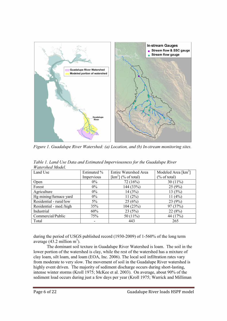
The Guadalupe River watershed is located in the Santa Clara Valley basin anddrains to Lower South San Francisco Bay (Figure 1). The watershed drainage areaencompasses approximately 444 km2 (170 mi2) and an elevation change from sea level tonearly 1,160 m (3,800 feet). The watershed includes six reservoirs, which are located inthe upper reaches of four of the tributaries in the watershed.

The watershed is approximately 46% developed urban area, 33% forest and 16%open area (Table 1). Only areas downstream from the reservoirs were dynamicallysimulated. Detailed land use statistics were also determined for this portion of thewatershed (Table 1) and indicate the downstream portion of the watershed is mostlydeveloped (75%), while the headwaters are mostly forested mountains.

The Guadalupe Watershed has a mild Mediterranean-type climate with a cool wetwinter season around 16°C (60°F) and a warm dry summer season around 27°C (80°F).The lower elevation areas receive an average of 380 mm (15 inches) of rainfall per year,while the upper elevations annually receive 1,000-1,500 mm (40-60 inches) ofprecipitation. On average, >90% of the annual rainfall occurs from November to Mayinclusively but there is large inter-annual variability in rainfall, e.g., 40% to 200% ofnormal in the Bay Area (McKee et al. 2003), resulting in an annual runoff variation


Figure 1. Guadalupe River Watershed: (a) Location, and (b) In-stream monitoring sites.

Table 1. Land Use Data and Estimated Imperviousness for the Guadalupe RiverWatershed Model.Land Use Estimated %

ImperviousEntire Watershed Area[km2] (% of total)

Modeled Area [km2](% of total)

Open 0% 72 (16%) 30 (11%)Forest 0% 144 (33%) 25 (9%)Agriculture 0% 14 (3%) 13 (5%)Hg mining/furnace yard 0% 11 (2%) 11 (4%)Residential - rural/low 5% 25 (6%) 23 (9%)Residential - med./high 35% 104 (23%) 97 (37%)Industrial 60% 23 (5%) 22 (8%)Commercial/Public 75% 50 (11%) 44 (17%)Total - 443 265

during the period of USGS published record (1930-2009) of 1-560% of the long termaverage (43.2 million m3).

The dominant soil texture in Guadalupe River Watershed is loam. The soil in thelower portion of the watershed is clay, while the rest of the watershed has a mixture ofclay loam, silt loam, and loam (EOA, Inc. 2006). The local soil infiltration rates varyfrom moderate to very slow. The movement of soil in the Guadalupe River watershed ishighly event driven. The majority of sediment discharge occurs during short-lasting,intense winter storms (Kroll 1975; McKee et al. 2003). On average, about 90% of thesediment load occurs during just a few days per year (Kroll 1975; Warrick and Milliman


2003; McKee et al. 2003; McKee et al. 2004). Suspended sediment concentrations areclosely correlated with flow in part because the extensive dry season essentially returnsthe system to the same initial condition by the start of the wet season (Krone 1979).Suspended sediment load in the Guadalupe River watershed, like most watersheds in theBay Area, appears to be transport-limited, rather than supply-limited.

Historic agricultural, mercury mining, and industrial activities and more recenturban development and population growth in the Guadalupe River watershed haveresulted in widespread distribution of contaminant sources in the watershed. Theinoperative mining district of New Almaden (within the Alameda Quicksilver CountyPark), which at one time was the largest supplier of mercury in North America, isresponsible for historic deposits of mercury that continue to flow to the Bay fromupstream areas via a drainage network (Thomas et al. 2002; Conoway et al. 2003). Inaddition, mercury from urban uses and atmospheric deposition continues from the lowerurbanized and impervious areas of the watershed. Although PCB manufacturing wasbanned in the late 1970s, PCB use during the 1950s and 1960s in power transmission,capacitors, hydraulic fluids, plasticizers, paints, and flame retardants left a legacy of theselong-lived compounds dispersed unevenly in urban environments (McKee et al. 2006b).

Model Description

The HSPF is a continuous, deterministic lumped-parameter model that simulateshydrologic and water quality processes on pervious and impervious land surfaces, instreams, and in well-mixed water bodies (Bicknell et al., 2001). The model generates atime history of the runoff flow rate, and sediment and contaminant concentrations for anypoint in the watershed being modeled.

The base modules of HSPF are PERLND, IMPLND, and RCHRES. PERLNDrepresents pervious land, IMPLND represents impervious land, and RCHRES representsstream segments (reaches) and water bodies (reservoirs). The PERLND modulecalculates infiltration and soil moisture storage, while IMPLND does not. The RCHREStreats stream segments as uni-directional and one-dimensional (i.e. as a well-mixedstream with a uniform cross-section).

The key hydrologic processes are infiltration and surface runoff generated fromprecipitation and irrigation. Infiltration drives subsurface flow, which contributes tostream flow, along with the surface runoff. Precipitation and surface runoff drivesoil/sediment detachment and transport. Suspended sediment is preferentially transportedby grain-size to channels, where it can be carried downstream by advection or depositedlocally to become bed sediment. Depending on the stream flow conditions and the shearstress levels, the bed sediment can accrete or erode. Contaminants can be modeled asrunoff-associated or sediment-associated or as both (in this current application). Therunoff-associated contaminant module functions as a basic build-up/wash-off model andcan include both wet and dry atmospheric deposition. The sediment-associatedcontaminant module assigns contaminant concentrations to soil/sediment, which istransported by runoff to channels. Particle size distribution and preferential transport areimplicitly incorporated by applying ratios to the sediment yield into channels. Once in-stream, clay, silt, and sand are modeled as separate constituents; however, bed load is not


modeled explicitly. In-channel contaminants can be transported by advection, can bedeposited or eroded (when sorbed to sediment), can undergo partitioning and decayprocesses. Several notable model simplifications for contaminant processes include nopartitioning in surface runoff and no speciation for user-defined constituents.

The BASINS system was used to delineate the overall watershed boundary andthe subbasin boundaries in the Guadalupe River Watershed using elevation from NationalElevation Dataset, drainage maps from National Hydrography Dataset (NHD-Plus), and alocal stormdrain catchment map and GIS data set developed by William Lettis &Associates, Inc. (WLA) in association with the Oakland Museum of California (OMC)and San Francisco Estuary Institute (SFEI). A major consideration in delineating in thewatershed boundary was the presence of six reservoirs in the headwaters area of thewatershed. To simplify the model, the watershed boundary was adjusted to excludereservoirs and their upstream watersheds. Reservoir releases and loads were thenincluded as point-source inputs into the appropriate stream locations. By delineating thewatershed in this way, the model was able to account for the influence of managedreservoir flows without having to model the internal dynamics of the reservoirsthemselves.

The Guadalupe River Watershed was subdivided into 12 model segments(“parameterization units”) containing 27 subbasins. The subbasin boundaries weremodified to coincide with monitored locations and areas of interest (e.g. former Hg minesand selected urban and non-urban areas). Land use, based on data sets from SCVWD andAssociation of Bay Area Governments (ABAG), was aggregated into nine categories:open, forest, agriculture, the historic Hg mining area (now the New Almaden QuicksilverCounty Park), the historic Hg furnace yard where the majority of ore was processed,rural/low-density residential, medium-/high-density residential, commercial/public, andindustrial areas.

The contaminants were treated in a simplified manner in the model. Mercuryexists in several forms in freshwater environments [Hg(0), Hg(II), and MeHg] and cyclesbetween these species. In this model, all species were treated as an aggregate [total-Hg].The chemical properties of Hg(II) were used for model parameterization since Hg(II) isthe dominant species (>99%) of Hg in Guadalupe River (data not shown). PCBs exist asa mixture of 209 congeners, which are present in varying amounts in the environment,depending on amounts manufactured (and subsequently released to the environment) aswell as congener persistence. In this model, PCBs were modeled as total-PCBs, i.e., sumof all congeners. The congener PCB-118, a pentachlorobiphenyl, was selected to providerepresentative properties as input to the model for several reasons: it has an intermediatechlorination level and, thus, intermediate chemical properties; it is abundant in Aroclor1254, which is the predominant Aroclor in San Francisco Bay samples (Johnson et al.2000); and it has similar chemical properties to PCB-126, the most toxic congener that isgenerally not measured due to its very low concentrations (Davis 2004).

Another model simplification was treating dissolved organic carbon (DOC)implicitly through incorporation into linear partition coefficients. In some Hg and PCBswatershed models (e.g. WARMF, DELPCB), DOC has been modeled explicitly sinceDOC concentrations normally have a strong impact on dissolved Hg and PCBconcentrations. This relationship appears more valid for watersheds where atmosphericdeposition is a major source of contamination and dissolved organic carbon plays a


dominant role in transport of Hg (Hurley et al., 1998; Grigal, 2002). In the GuadalupeRiver, we find only weak relationships between DOC and Hg as well as PCBs. Perhapsbecause the majority of the mercury contamination is sediment-associated from miningsources and the majority of the PCB contamination is sediment-associated from industrialsources. Therefore implicit treatment of DOC through the use of partition coefficientsappears reasonable for the Guadalupe River application.

Data Collation

Hydrologic model performance is highly dependent on the accuracy and qualityof precipitation data. Especially in a watershed with large elevation changes (near sea-level to approximately 3000 feet in the modeled portion of the Guadalupe Riverwatershed), rainfall tends to vary greatly with location and time. Therefore, high qualityprecipitation data with high temporal and spatial resolution were needed. Fortunately, theGuadalupe River watershed contained high-resolution rainfall gauges well distributedspatially and at a wide range of elevations.

High-resolution precipitation data (15-minute intervals) were obtained from SantaClara Valley Water District (SCVWD) for five precipitation gauges located within thewatershed and one gauge just outside. The time period of the rainfall data was chosen tooverlap with Guadalupe River sediment and contaminant data sets. Hourly referenceevapotranspiration data were obtained for Morgan Hill from California IrrigationManagement Information Systems (CIMIS) and monthly pan evaporation data from theLos Alamitos Recharge Facility in San Jose were obtained from SCVWD.

Stream flow records (15-minute intervals) were obtained from the USGS andSCVWD for numerous gauges in the watershed (Figure 1) for October 1994 toSeptember 2007. Additionally, reservoirs release and diversion records were obtained touse as point sources and sinks in the model. Another water source for the watershed wasurban irrigation, however, irrigation time series data were not available and instead wereestimated from precipitation and evapotranspiration records using methodology fromAQUA TERRA Consultants (2006). Agricultural irrigation was not treated since less than5% of the watershed is dedicated to agriculture.

Suspended sediment records (15-minute intervals) were obtained from SFEI andUSGS for the wet seasons of water years 2003 to 2007 for the SSC gauge (USGS#11169025) (Figure 1). Additionally, sediment load time series were developed for thereservoirs as point sources into the model based on reservoir release grab samplescollected for the Guadalupe TMDL (Tetra Tech, Inc. 2003). Unfortunately, no SSCrecords were available for the major tributaries.

Mercury and PCB concentration data for calibration and validation purposes werecompiled from SFEI’s Guadalupe River sampling program (e.g. McKee et al. 2006b).SFEI’s Guadalupe River sampling program collected Hg and PCBs samples fromWY2003-2006 and 2010 at the SSC gauge site (USGS #11169025) and at a second siteupstream (USGS #11167800) during WY 2010 only (McKee et al. unpublished data).Water samples were collected using a FISP D-95 water quality sampler from bridgesusing a crane and winch during non-wading stages and by dipping clean prepared samplebottles below the surface in the deepest point of each stream location during wadingstages. Roughly 90% of the samples were collected during storm flow. One liter samples


for Hg analysis were analyzed for total Hg with cold vapor atomic fluorescence followingU.S. EPA method 1631e (USEPA 2002) at San Jose State University Moss LandingMarine Laboratories. A subset of samples were also analyzed for dissolved mercuryspecies. Four liter samples for PCBs were analyzed for 40 congeners using high-resolution gas chromatography / high-resolution mass spectrometry (HRGC/HRMS)following EPA method 1668 revision A (USEPA 1999) at AXYS Analytical ServicesLtd, Sidney British Columbia, Canada.

Mercury load time series were developed for the reservoirs as point sources intothe model based on reservoir release grab samples collected for the Guadalupe TMDL(Tetra Tech, Inc. 2003). Most of the grab samples were taken from low flow events(controlled releases). The reservoirs contributions of sediment and mercury duringuncontrolled releases were a major data gap. During low flow releases, the reservoirscontributed little sediment-associated mercury since the most of the reservoir releaseshave very low sediment concentrations (1-10 mg/L); however the reservoirs were animportant source of dissolved mercury into the watershed. PCB reservoir loads were notmodeled due to PCBs’ tendency to strongly sorb to sediment and the low sedimentconcentrations in the reservoir releases. Unfortunately, there were no data to support orcontradict this assumption. Wet and dry atmospheric deposition sources were includedfor both mercury and PCBs (Tables 2 and 3). For mercury, local deposition data wereavailable, but for PCBs, national data were used.

Initial Parameterization

To the extent possible, initial model parameters were obtained from literature,with preference given to local information. Initial hydrology parameters relied heavily onlocal HSPF hydrology modeling reports (Aqua Terra Consultants 2006; Clear CreekSolutions, Inc. 2007), as well as BASINS Technical Note 6: Estimating Hydrology andHydraulic Parameters for HSPF (USEPA 2000). Initial sediment parameter data werebased on local soil data (EOA 2006) and the HSPF Parameter Database (HSPFParm)(USEPA 1999), which had parameters for a watershed in the same county (CalabazasCreek, Santa Clara County, CA). Additionally, bed sediment grain-size data wereobtained from USGS for the downstream gauge site.

Table 2. Parameter Values for Mercury Simulation.Parameter Description (units) Values used Ref.POTFW Detached sediment potency factor (lbs/ton) 2*10-5 – 0.152 1; 2POTFS Soil matrix scour potency factor (lbs/ton) 2*10-6 – 0.0152 1; 2ACQOP Rate of accumulation (lbs/ac*day) 1*10-8 – 2*10-8 3SQOLIM Maximum storage (lbs/ac) 1*10-6 3WSQOP Runoff value for 90% removal/hour (in/hr) 1.5 4ADPM1 Linear partition coefficient (L/mg) 0.001 – 0.08 5; 6ADPM2 Adsorption/desorption rate (1/day) 0.1 – 0.2 7ADFX Dry atmospheric deposition (lbs/ac*day) 4.6*10-7 8ADCN Wet atmospheric deposition (mg/L in rain) 9.7*10-6 81 – LWA 2006; 2 – Tetra Tech 2005; 3 – Gersberg et al. 2000; 4 – Carleton and Cocca 2004; 5 – Allisonand Allison; 6 - Wetzel 2005; 7 – Aqua Terra 2009; 8 – Tsai and Hoenicke 2001


Table 3. Parameter Values for PCBs Simulation.Parameter Description (units) Values used Ref.

POTFW Detached sediment potency factor (lbs/ton) 4.4*10-6 – 8*10-4 1POTFS Soil matrix scour potency factor (lbs/ton) 4.4*10-7 – 8*10-5 1SQOLIM Maximum storage (lbs/ac) 1*10-6 2ADPM1 Linear partition coefficient (L/mg) 0.00676 – 0.0676 3ADPM2 Adsorption/desorption rate (1/day) 0.001 – 0.1 Calib.FSTDEC First order decay rate (1/day) 0.0057 4KSUSP/KBED Sediment-associated decay rate (1/day) 0.008 4ADFX Dry atmospheric deposition (lb/ac*day) 1.2*10-7 5ADCN Wet atmospheric deposition (mg/L in rain) 2*10-6 51 – McKee et al. 2006; 2 – Gersberg et al. 2000; 3 – Hansen et al. 1999; 4 – Mackay et al. 1992; 5 – Park etal. 2001

Since no HSPF parameter data are available for Hg or PCBs in the existingpublished literature, a broader literature search was performed to gather chemicalproperties data on each contaminant, as well as known and expected concentrations datafor soils and sediments. The references for the parameters used are listed (Tables 2 and3). For mercury, the model’s soil and bed sediment components were parameterizedusing local data on mercury concentrations in soils and bed sediment from the GuadalupeTMDL (Tetra Tech, Inc. 2003). No data were found for PCBs in soils for GuadalupeWatershed, so the PCB model soil parameterization relied on a review of world literatureon PCBs concentration in soils by land use category (McKee et al. 2006c). PCBs in bedsediment concentrations were guided by data on PCBs in bed sediment from a number ofstorm drainages in Santa Clara County (KLI 2002; Yee and McKee 2010).

Calibration and Validation Process

Calibration of a HSPF model is an iterative process of making parameter changesand sometimes model set-up changes, running the model and comparing the simulatedmodel outputs to observed data or literature values. The standard procedure is to calibratehydrology first, then hydraulics and sediment, and finally contaminants. The HSPFcalibration procedure is well documented by Donigian (2002).

The hydrologic model was calibrated at two upstream locations and validated atthe most downstream gauge. Two Guadalupe River tributaries with very differentsurrounding landscapes were chosen as upstream calibration sites. The first, GuadalupeCreek, flows from a steep undeveloped area. The second, Canoas Creek, flows through amostly flat mixed-development area. Additionally, Guadalupe Creek is reservoirinfluenced whereas Canoas Creek is not reservoir influenced. The hydrologic model wascalibrated using comparisons between observed and simulated instantaneous discharge atthe hourly and daily time step, monthly and annual flow volumes, and long-term flowduration curves.

The hydraulic model was calibrated by comparing simulated and observed flowvelocity and simulated and observed velocity-discharge relationships. Stage, velocity and


discharge data were available for two locations on the Guadalupe River, allowing forcalibration of the model’s stage-volume-discharge tables for the main stem of the river.The data set was not large enough to validate the hydraulic calibration. Since no stageand flow velocity data were available for the tributaries, their stage-volume-dischargetables were adjusted according to expected behavior.

The sediment model was calibrated to a suite of local data, literature values andexpected behaviors. The soil/sediment erosion model was calibrated to local estimates ofsediment yields calculated for each model segment and land use. The sediment yieldtarget values were based on local estimates of sediment production rates for different landuse types (Lewicki and McKee 2009) that were scaled by an area-based delivery ratio.The in-stream sediment model was calibrated at the downstream site using comparisonsbetween observed and simulated instantaneous suspended sediment concentrations at thehourly and daily time step and instantaneous grain size distributions. Suspended sedimentdata at the downstream site was available for WY2003-2007, and was split into WY2003-2005 for calibration and WY2006-2007 for validation. The sediment model was alsocalibrated to expected bed behavior for known areas of accretion or erosion. A majorlimitation in the sediment calibration data set was the lack of SSC records for thetributaries.

Similar to the sediment model, the contaminant models were calibrated to acombination of local data and data from published literature. The land-based contaminantmodels were calibrated to target Hg and PCBs yields calculated by land use (Mangarellaet al. 2006). The in-stream contaminant models were calibrated to instantaneoussuspended contaminant concentrations (grab sample data) and to bed sedimentcontamination data. For both Hg and PCBs, contaminant grab sample data were availablefor WY2003-2006, and were split into WY2003-2004 for calibration and WY2005-2006for validation. For the calibration period, 62 Hg and 39 PCBs concentration data pointswere available. For the validation period, 101 Hg and 26 PCBs concentration data pointswere available. Additionally, Hg grab sample data were available for numerous upstreamlocations (e.g., all of the major tributaries to Guadalupe River) during the modeledperiod, although these were generally small data sets (2-25 samples). These upstreamdata sets provided spatial resolution and were used to refine the Hg calibration.

Model Evaluation

The model was evaluated using recommended statistical measures andperformance metrics (Donigian 2002; Moriasi et al. 2007). The model was run on a 15-minute time step from WY 1995 to 2007 with the first year of data repeated as a spin-upyear to initialize the model. The results of the spin-up year were excluded from the modelevaluation. Calibration and validation statistics were calculated for daily flow volume anddaily suspended sediment concentration. To better assess model accuracy, theperformance was evaluated separately for storm events and baseflow conditions. For thecontaminants, calibration and validation statistics were calculated for the pairedsimulated concentrations and grab samples (rounded to the nearest hour). Most of thegrab samples were taken during storm events, so the data were not separated for stormevents and baseflow conditions.


The following statistics were used to evaluate model performance:• Coefficient of determination (R2)• Percent bias (PBIAS)• Ratio of root mean square error to the standard deviation of measured data (RSR)• Nash-Sutcliffe efficiency (NSE)

Donigian (2002) provided the following model evaluation criteria for the coefficient ofdetermination for daily streamflow: above 0.8 is ‘very good’ model performance,between 0.7 and 0.8 is ‘good’ model performance, between 0.6 and 0.7 is ‘fair’ modelperformance, and below 0.6 is ‘poor’ model performance. Moriasi et al. (2007)established the following model evaluation guidelines for watershed simulations: modelperformance can be judged satisfactory if NSE > 0.50 and RSR ≤ 0.70, and if PBIAS±25% for streamflow, PBIAS ±55% for sediment, and PBIAS ±70% for contaminants.

RESULTS AND DISCUSSION

Hydrologic Simulation

The hydrologic model calibration resulted in parameters being adjusted by landuse type, hydrologic soil group and slope. The final calibrated key hydrologic parametersare shown Table 4 along with typical values for comparison. The statistical evaluation ofthe hydrologic model calibration and validation are shown in Table 5. For both thecalibration and validation, the model exhibited satisfactory performance for storm events,meeting all model performance criteria from Moriasi et al. (2007). The model performedless well for baseflow conditions, but still met the satisfactory performance criteria forGuadalupe Creek and Guadalupe River. The model failed the satisfactory performancecriteria for baseflow conditions for Canoas Creek. However, inspection of the CanoasCreek flow record showed the low-flow/dry season gauge records were unreliable, forexample, occasionally early or late season storms were missed due to the gauge beingoffline or otherwise non-responsive.

For the watershed as a whole, the model simulated daily streamflow very well(Figure 2a), exhibiting a nearly 1-to-1 relationship with a coefficient of determination of0.95. Additionally, the model was able to capture behavior of storms on an hourly basis(data not shown).

Table 4. Parameter Values for Hydrologic Simulation.Parameter Description Values used Typical range*LZSN Lower zone nominal storage (in) 4.0 – 14.0 3.0 – 8.0INFILT Soil infiltration capacity index (in/hr) 0.04 – 0.12 0.01 – 0.25AGWRC Groundwater recession coefficient (1/day) 0.92 – 0.99 0.92 – 0.99UZSN Upper zone nominal storage (in) 0.5 – 1.5 0.1 – 1.0DEEPFR Fraction of groundwater inflow to deep

recharge0.1 – 0.3 0.0 – 0.2

LZETP Lower zone ET parameter 0.5 – 0.95 0.2 – 0.7INTFW Interflow inflow parameter 0.5 – 2.5 1.0 – 3.0IRC Interflow recession parameter 0.3 – 0.8 0.5 – 0.7CEPSC Interception storage capacity (in) 0.1 – 0.3 0.03 – 0.20*from BASINS Technical Note 6 (USEPA 2000)


Table 5. Hydrologic Simulation Results: Comparing observed and simulated daily flow(cfs).

WY 1995-2007 R2 % Bias RSR NSECalibration site #1: storm 0.86 -16 0.39 0.85Canoas Creek baseflow 0.37 -54 1.9 -2.6Calibration site #2: storm 0.88 19 0.44 0.81Guadalupe Creek baseflow 0.78 -0.9 0.47 0.78Validation site: storm 0.93 -10 0.27 0.93Guadalupe River (USGS#11169025) baseflow 0.78 -8.7 0.52 0.73

Figure 2. Comparison of Observed and Simulated Values: (a) Daily streamflow(WY1995-2007), (b) Daily sediment (WY2003-2007), (c) Mercury grab samples(WY2003-2006), and (d) PCBs grab samples (WY2003-2006).


Sediment Simulation

The sediment model calibration was limited to adjusting parameters to achievegeneral “expected behavior” in the tributaries and looking at overall results at the bottomof the watershed where data was available. The key sediment parameters used are shownin Table 6 along with typical values for comparison. The statistical evaluation of thesediment model calibration and validation are shown in Table 7. For both the calibrationand validation, the model exhibited satisfactory performance for storm events, meetingall model performance criteria from Moriasi et al. (2007). The model performed poorlyfor baseflow conditions, exhibiting strong bias towards over-simulating sedimentconcentrations. Evaluating the sediment model over the entire period of data collectionshows a large degree of scatter at the higher SSC values (Figure 2b), suggesting that themodel is performing less well during storm events than the data in Table 7 would suggest.

Table 6. Parameter Values for Sediment Simulation.Parameter Description (units) Values used Typical range*KRER Coefficient in the soil detachment equation 0.25 – 0.30 0.15 – 0.45JRER Exponent in the soil detachment equation 2 1.5 – 2.5AFFIX Daily reduction in detached sediment (1/day) 0.0 – 0.05 0.03 – 0.1COVER Fraction of land surface protected from

rainfall0.60 – 0.97 0.0 – 0.90

NVSI Atmospheric additions to sediment storage(lbs/ac*day)

0.0 – 2.0 0.0 – 5.0

KSER Coefficient in the detached sediment washoffequation

0.4 – 2.0 0.5 – 5.0

JSER Exponent in the detached sediment washoffequation

2 1.5 – 2.5

KGER Coefficient in the soil matrix scour equation 0.0- 0.06 0.0 – 0.5JGER Exponent in the soil matrix scour equation 1.0 1.0 – 3.0KEIM Coefficient in the solids washoff equation 0.5 0.5 – 5.0JEIM Exponent in the solids washoff equation 2.0 1.0 – 2.0ACCSDP Solids accumulation rate on impervious

surface (lbs/ac*day)0.001 – 0.01 0.0 – 2.0

REMSDP Fraction of solids removed per day 0.03 – 0.05 0.03 – 0.2KSAND Coefficient in the sandload power function 0.15 – 0.3 0.01 – 0.5EXPSAND Exponent in the sandload power function 2.1 – 3.0 1.5 – 3.5W Fall velocity in still water (in/s) 0.00004 –

0.00120.0001 – 4.0

M Erodibility coefficient of the sediment(lbs/ft2*day)

0.01 0.01 – 2.0

TAUCD Critical bed shear stress for deposition(lbs/ft2)

0.08 – 0.27 0.01 – 0.30

TAUCS Critical bed shear stress for scour (lbs/ft2) 0.18 – 0.32 0.05 – 0.50*from BASINS Technical Note 8 (USEPA 2006)


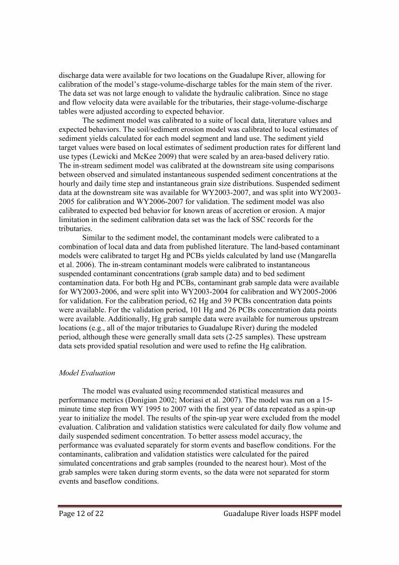
Table 7. Sediment Simulation Results: Comparing observed and simulated dailysuspended sediment concentrations (mg/L).

N R2 % Bias RSR NSECalibration storm 145 0.73 -11 0.55 0.70(WY 2003-05) baseflow 554 0.50 -134 1.18 -0.38Validation storm 120 0.81 -23 0.49 0.76(WY 2006-07) baseflow 335 0.66 -130 1.00 0.01

Contaminant Simulation

Due to the strongly sediment-associated nature of both mercury and PCBs, modelcalibration was hindered by the poor performance of the sediment model. Withoutconfidence in the underlying model driving the contaminant transport, any calibrationadjustments might be compensation for problems in the underlying model. Tables 2 and 3provide the key parameters for mercury and PCBs, respectively. For the reasonsexplained above, parameters were not modified from literature values. Tables 8 and 9document the poor performance of the contaminant models; in all years evaluated theNash-Sutcliffe efficiency is below zero, which means the simulated values are worsepredictors than the average of the observed data points. Figures 2c and 2d show the linearregression of each contaminant model over the entire period of data collection. Themercury model exhibits an extremely poor regression relationship in part due to twounusually high Hg grab sample values (both are from December 2002 when there mayhave been mass wasting events in the former Hg mining area). The PCB model exhibits abetter regression relationship, but still there is a large degree of scatter in the relationship.

Table 8. Mercury Simulation Result: Comparing observed grab samples andcorresponding simulated values (ng/L).

Water Year N R2 % Bias RSR NSECalibration 2003 26 0.02 70 1.14 -0.29

2004 36 0.25 -40 2.20 -3.85Validation 2005 52 0.001 -63 2.04 -3.16

2006 49 0.03 -94 2.52 -5.37

Table 9. PCBs Simulation Results Comparing observed grab samples and correspondingsimulated values (ng/L).

Water Year N R2 % Bias RSR NSECalibration 2003 21 0.03 34 1.51 -1.27

2004 18 0.42 33 1.58 -1.49Validation 2005 12 0.11 -43 1.59 -1.52

2006 14 0.08 -108 2.58 -5.66


CONCLUSIONSA high-resolution hydrology model was successfully developed for the Guadalupe

River Watershed. The hydrology model was then extended to include sediment, but washindered by a lack of calibration data in the tributaries. Initial parameters for mercury andPCB models were developed and applied to the (unsatisfactory) sediment model. As bothcontaminant models were reliant on the sediment model, their calibration andperformance were limited by the sediment model needing improvement. If the sedimentmodel were improved to satisfactory state, the contaminant models could be re-visitedand potentially improved to an acceptable level of performance to forecast loads andimpacts of management actions.

Recommendations

The recommendations for improving the model for both sediment andcontaminants are to collect supporting data related to hydraulics, concentrations, andgrain-size distribution and to have the model reviewed by an expert in sediment transport.Specifically, the ideal data set to support improvement of the model would be:

• stream cross-sections and stage-area-discharge-velocity relationships for all majortributaries

• SSC data for major tributaries (at minimum should have SSC data for reachesrepresenting different sediment transport types, e.g., reservoir-fed steep reaches,non-reservoir-fed steep reaches, flatland reaches, urban reaches)

• sediment grain size data for reaches representing different sediment transporttypes

• sediment and contaminant concentration data for high-flow reservoirreleases/spills

• generally improve local data sets for PCBs in relation to soils, and for PCBs andHg in relation to grain sizes in both bed sediment and suspended sediment inflowing water.

REFERENCES

Ackerman, D., Schiff, K.C., and S.B. Weisberg, 2005. Evaluating HSPF in an arid,urbanizing watershed. Journal of the American Water Resources Association 41(2):477-486.

Ackerman, D. and E. Stein, 2008. Evaluating the effectiveness of best managementpractices using dynamic modeling. Journal of Environmental Engineering 134(8): 628-639.

AQUA TERRA Consultants, 2006. Hydrologic Modeling of the Castro Valley Creek andAlameda Creek Watersheds with the U. S. EPA Hydrologic Simulation Program –FORTRAN. Final Report. Prepared for the Alameda Countywide Clean Water Program,Hayward, CA. January 2006.


Austin, C. and R. Looker, 2006. Mercury in San Francisco Bay: Proposed Basin PlanAmendment and Staff Report for Revised Total Maximum Daily Load (TMDL) andProposed Mercury Water Quality Objectives. California Regional Water Quality ControlBoard San Francisco Bay Region, August 1st, 2006. 116pp.

Bergman, M.J., Green, W., and L.J. Donnangelo, 2002. Calibration of storm loads in theSouth Prong watershed, Florida, using BASINS/HSPF. Journal of the American WaterResources Association 38(5):1423-1436.

Bicknell, B.R., Imoff, J.C., Kittle, J.L., Jobes, T.H., and A.S. Donigan, 2001.Hydrological Simulation Program – FORTRAN. Version 12. User’s Manual, AQUATERRA Consultants. United States Environmental Protection Agency.

Bledsoe, B.P. and C.C. Watson, 2001. Effects of urbanization on channel stability.Journal of the American Water Resources Association 37(2): 255-270.

Booth, D.B., 1990. Stream-channel incision following drainage basin urbanization. WaterResources Bulletin. 26:407–17.

Clear Creek Solutions, Inc., 2007. Bay Area Hydrology Model User Manual. Preparedfor Alameda Countywide Clean Water Program, San Mateo Countywide Water PollutionPrevention Program, and Santa Clara Valley Urban Runoff Pollution PreventionProgram. July 2007.

Clear Creek Solutions, Inc., 2007. Hydrologic Modeling of Santa Clara CountyWatersheds with the U.S. EPA Hydrologic Simulation Program – FORTRAN (HSPF).Final Report. Prepared for Santa Clara Valley Urban Runoff Pollution PreventionProgram. October 2007.

OEHHA 1999. California Sport Fish Consumption Advisories 1999. Pesticide andEnvironmental Toxicology Branch Office of Environmental Health Hazard AssessmentCalifornia Environmental Protection Agency. Oakland, California.

OEHHA, 2011. Health Advisory and Safe Eating Guidelines for San Francisco Bay Fish& Shellfish. Pesticide and Environmental Toxicology Branch Office of EnvironmentalHealth Hazard Assessment California Environmental Protection Agency. Oakland,California. 47pp.

Conaway, C.H., S. Squire, R.P. Mason, and A.R. Flegal. 2003. Mercury Speciation in theSan Francisco Bay Estuary. Marine Chemistry, Vol. 80, pp. 199-225.

David, N., Gluchowski, D.C, Leatherbarrow, J.E, Yee, D., and McKee, L.J, in review.Evaluation of loads of mercury, selenium, PCBs, PAHs, PBDEs, dioxins, andorganochlorine pesticides from the Sacramento-San Joaquin River Delta to San FranciscoBay.


David, N., McKee, L.J., Black, F.J., Flegal, A.R., Conaway, C.H., Schoellhamer, D.H.,Ganju, N.K., 2009. Mercury concentrations and loads in a large river system tributary toSan Francisco Bay, California, USA. Environmental Science and Technology, Vol. 28,No. 10, pp. 2091–2100.

Davis, J., D. Yee, J. Collins, S. Schwarzbach, and S. Luoma, 2003. Potential forIncreased Mercury Accumulation in the Estuary Food Web. San Francisco Estuary andWatershed Science, pp. 1 to 8.

Davis, J.A., 2004. The long-term fate of polychlorinated biphenyls in San Francisco Bay(USA). Environmental Toxicology and Chemistry 23(10): 2396-2409.

Davis, J.A., Hetzel, F., Oram, J.J., and McKee, L.J., 2007. Polychlorinated biphenyls(PCBs) in San Francisco Bay. Environmental Research, Vol. 105, pp. 67-86.

Dean, J.D., Meier, D.W., Bicknell, B.R. and A.S. Donigian, Jr. 1985. Simulation of DDTTransport and Fate in the Arroyo Colorado Watershed, Texas. Prepared for USEPA,Environmental Research Laboratory, Athens, GA. August 1985.

Donigian, A.S., 2002. Watershed Model Calibration and Validation: The HSPFExperience. WEF-National TMDL Science and Policy, November 13-16, 2002. PhoenixAZ, WEF-2002 Specialty Conference Proceedings on CD-ROM.

Donigian, A.S. and B.R. Bicknell, 2007. Modeling the Contribution of Copper fromBrake Pad Wear Debris to the San Francisco Bay. Prepared for Association of Bay AreaGovernments San Francisco Estuary Project and California Department ofTransportation.

EOA, Inc. 2006. C.3 Stormwater Handbook. Prepared for Santa Clara Valley UrbanRunoff Pollution Prevention Program. Original Report May 2004. Updated Report May2006. 210pp.

Fontaine, T.A. and V.M.F. Jacomino, 1997. Sensitivity analysis of simulatedcontaminated sediment transport. Journal of the American Water Resources Association33(2):313-326.

Gersberg, R.M.; Pitt, J.; King, A.; Johnson, H. and R. Wright, 2000. Use of theBASINS Model to Estimate Loading of Heavy Metals from the Binational Tijuana RiverWatershed. Proceedings of the Water Environment Federation, Watershed 2000, pp. 234-243(10).

Gilbreath, A.N., Yee, D., and McKee, L.J. (in review). Concentrations and loads of tracecontaminants in a small urban tributary, San Francisco Bay, CA. Science of the TotalEnvironment.


Grigal, D.F., 2002. Inputs and outputs of mercury from terrestrial watersheds: a review.Environmental Reviews 10, 1-39.

Hummel, P.R., Kittle, J.L., Duda, P.B. and A. Patwardhan, 2003. Calibration of aWatershed Model for Metropolitan Atlanta. Proceedings of the Water EnvironmentFederation, National TMDL Science and Policy 2003, pp. 781-807(27)

Hurley, J.P., Cowell, S.E., Shafer, M.M., and Hughes, P.E., 1998. Partitioning andtransport of total and methyl mercury in the lower Fox River, Wisconsin. Environment,Science and Technology 32, 1424-32.

Im, S., Brannan, K.M., and S. Mostaghimi, 2003. Simulating hydrologic and waterquality impacts in an urbanizing watershed. Journal of the American Water ResourcesAssociation 39(6):1465-1479.

Johnson, G.W., Jarman, W.M., Bacon, C.E., Davis, J.A., Ehrlich, R., and R.W.Risebrough, 2000. Resolving polychlorinated biphenyl source fingerprints in suspendedparticulate matter of San Francisco Bay. Environmental Science and Technology 34(4):552-559.

KLI, 2002. Joint stormwater agency project to study urban sources of mercury, PCBs andorganochlorine pesticides. Final Report. Prepared by Kinnetic Laboratories, Inc. SantaCruz, CA. April 2002.

Kroll, C. G. 1975. Estimate of sediment discharges, Santa Ana River at Santa Ana andSanta Maria River at Guadalupe California. U.S. Geol. Surv., Water-ResourcesInvestigations 40-74.

Krone, R.B. 1979, Sedimentation in the San Francisco Bay system, in San Francisco Bay:The Urbanized Estuary, edited by T.J. Conomos, pp. 85–96, Pacific Division of theAmerican Association for the Advancement of Science, San Francisco, CA.

Larry Walker Associates, 2006. Calleguas Creek Watershed Metals and SeleniumTMDL: Draft Final Technical Report. Prepared on behalf of the Calleguas CreekWatershed Management Plan. Submitted to Los Angeles RWQCB and USEPA. March2006.

Lent, M.A. and L.J. McKee, 2011. Development of regional contaminant load estimatesfor San Francisco Bay Area tributaries based on annual scale rainfall-runoff and volume-concentration models: Year 1 results. A technical report for the Regional MonitoringProgram for Water Quality. San Francisco Estuary Institute, Oakland, CA.

Lewicki, M. and L.J. McKee, 2009. Watershed specific and regional scale suspendedsediment loads for Bay Area small tributaries. A technical report for the SourcesPathways and Loading Workgroup of the Regional Monitoring Program for WaterQuality: SFEI Contribution #566. San Francisco Estuary Institute, Oakland, CA. 28 pp +


Appendices.

Mangarella, P., Steadman, C., and L. McKee, 2006. Task 3.5.1: Desktop evaluation ofcontrols for polychlorinated biphenyls and mercury load reduction. A Technical Reportof the Regional Watershed Program. San Francisco Estuary Institute, Oakland, CA.

McKee, L., Leatherbarrow, J., Pearce, S., and Davis, J., 2003. A review of urban runoffprocesses in the Bay Area: Existing knowledge, conceptual models, and monitoringrecommendations. A report prepared for the Sources, Pathways and Loading Workgroupof the Regional Monitoring Program for Trace Substances. SFEI Contribution 66. SanFrancisco Estuary Institute, Oakland, CA.

McKee, L., Leatherbarrow, J., Eads, R., and Freeman, L., 2004. Concentrations and loadsof PCBs, OC pesticides, and mercury associated with suspended sediments in the lowerGuadalupe River, San Jose, California. A Technical Report of the Regional WatershedProgram: SFEI Contribution #86. San Francisco Estuary Institute, Oakland, CA.

McKee, L., Oram, J., Leatherbarrow, J., Bonnema, A., Heim, W., and Stephenson, M.,2006a. Concentrations and loads of mercury, PCBs, and PBDEs in the lower GuadalupeRiver, San Jose, California: Water Years 2003, 2004, and 2005. A Technical Report ofthe Regional Watershed Program: SFEI Contribution 424. San Francisco EstuaryInstitute, Oakland, CA.

McKee, L., Mangarella, P., Williamson, B., Hayworth, J., and L. Austin, 2006b. Reviewof methods to reduce urban stormwater loads: Task 3.4. A Technical Report of theRegional Watershed Program: SFEI Contribution #429. San Francisco Estuary Institute,Oakland, CA.

Moore, L.W., Matheny, H., Tyree, T., Sabatini, D., and S.J. Klaine, 1988. Agriculturalrunoff modeling in a small west Tennessee watershed. Journal of Water Pollution ControlFederation 60(2): 242-249.

Moriasi, D.N., Arnold, J.G., Van Liew, M.W., Binger, R.L., Harmel, R.D. and T.L.Veith, 2007. Model evaluation guidelines for systematic quantification of accuracy inwatershed simulations. Transactions of the ASABE 50(3):885-900.

Parker, R., Arnold, J.G., Barrett, M., Burns, L., Carrubba, L., Neitsch, S.L., Synder, N.J.,and R. Srinivasan, 2007. Evaluation of three watershed-scale pesticide environmentaltransport and fate models. Journal of the American Water Resources Association43(6):1424:1443.

SFBRWQCB, 2008. Total Maximum Daily Load for PCBs in San Francisco Bay FinalStaff Report for Proposed Basin Plan Amendment. San Francisco Bay Regional WaterQuality Board, Oakland, CA.


Shirian-Orlando, A.A. and C.G. Uchrin, 2007. Modeling the hydrology and water qualityusing BASINS/HSPF for the upper Maurice River watershed, New Jersey. J Env Sci andHealth, Part A. 42(3):289-303.

Tetra Tech, Inc. 2003. Technical Memorandum 2.2 Synoptic Survey Report.Guadalupe River Watershed Mercury TMDL Project. Prepared for Santa ClaraValley Water District. Prepared by Tetra Tech, Inc. September 2003.

Tetra Tech, Inc., 2005. Guadalupe River Watershed Mercury TMDL project: TechnicalMemorandum 5.3.2 – Data collection report. Volume I. Prepared for Santa Clara ValleyWater District. Prepared by Tetra Tech, Inc. February 2005.

Thomas, M.A., Conaway, C.H., Steding, D.J., Marvin-DiPasquale, M., Abu-Saba, K.E.,and Flegal, A.R., 2002. Mercury contamination from historic mining in water andsediment, Guadalupe River and San Francisco Bay, California. Geochemistry:Exploration, Environment, Analysis 2, 1-7.

USEPA, 1999. HSPFParm: An interactive database of HSPF model parameters, Version1.0. EPA-823-R-99-004, April 1999.

USEPA, 2000. BASINS Technical note 6: Estimating hydrology and hydraulicparameters for HSPF. EPA-823-R-00-012, July 2000.

USEPA, 2001. Better Assessment Science Integrating Point and Non-point Sources:BASINS 3.0 Users Manual. EPA 823-B-01-001, June 2001.

USEPA, 2006. BASINS Technical note 8: Sediment parameter and calibration guidancefor HSPF. EPA-68-C-01-037, January 2006.

Warrick J.A. and J.D. Milliman. 2003. Hyperpycnal sediment discharge from semiaridsouthern California rivers: implications for coastal sediment budgets. Geology.31(9):781-784.

guadalupe river watershed loading hspf model: year · pdf fileguadalupe river watershed...

Documents