guidance for determining applicability ... - water … include advanced capabilities for simulation...

1 Guidance for Determining Applicability of OWHM and GSFLOW May 18, 2017

Guidance for determining applicability of the USGS GSFLOW and OWHM models for hydrologic simulation and analysis

Summary

Over the past decade the U.S. Geological Survey (USGS) has developed two numerical codes that include advanced capabilities for simulation of groundwater and surface-water systems—the coupled Groundwater and Surface-water FLOW model (GSFLOW) model and the One-Water Hydrologic Flow Model (OWHM). Both codes are referred to as ‘integrated hydrologic models’ and both are based on MODFLOW-2005 and MODFLOW-NWT. Although the two codes have many similar capabilities, and can meet similar needs in some cases, there are important differences in the functionality, applicability, development history, and user support between the codes that may make them better suited to particular hydrologic settings or water-management issues. This guidance document describes key similarities and differences between the two codes as they relate to coupled groundwater/surface-water/landscape processes and water-resources management, and provides examples of the types of water-resource issues to which the codes have been applied. The following items summarize the discussion provided in the document:

• GSFLOW is a coupled groundwater/surface-water model based on MODFLOW and the PRMS watershed-modeling system. The coupled model represents three inter-connected regions and associated hydrologic processes: (1) the land surface, from plant canopy through the soil zone; (2) surface-water features (streams, lakes, ponds); and (3) unsaturated and saturated subsurface zones.

• OWHM includes the Farm Process for MODFLOW for simulating the use and movement of water across irrigated and other landscapes. OWHM also incorporates several additional MODFLOW capabilities from various independent versions of MODFLOW such as the subsidence and seawater-intrusion packages and local-grid refinement capability that are not currently available in GSFLOW. The core concept of the Farm Process is to internally calculate crop irrigation requirements (crop demands) and to then allocate surface-water and groundwater irrigation supplies to meet those demands that cannot be met by precipitation or root uptake from groundwater.

• Both codes use the time-step and stress-period concepts of MODFLOW, but there are important differences between the codes with respect to the minimum time step that can be simulated. GSFLOW uses daily time steps. The Farm Process assumes well managed crop irrigation and steady-state soil-moisture conditions. Because of this steady-state soil-moisture assumption, applications of the Farm Process must use time steps that are a minimum of several days; in practice, most applications of the code have used time steps of two weeks.

• Both models have capabilities for the user to specify many types of water-management conditions such as streamflow diversions and groundwater withdrawals to meet agricultural, municipal, and industrial needs; aquifer storage and recovery systems; and farm-conveyance systems. OWHM, however, has several additional options to constrain and prioritize water-supply deliveries, to internally calculate surface-water and


groundwater deliveries needed to meet water-supply demands, and to simulate transient land uses and land ownership of developed and native landscapes.

• Both models have limitations in how they simulate real-world hydrologic systems, but the watershed-simulation processes and daily time-step discretization available in GSFLOW make it possible to simulate hydrologic processes such as overland runoff, snowpack dynamics, soil-zone processes, recharge, surface-depression storage, and streamflow more comprehensively and in a more physically-based manner than those available in OWHM. Because of this, GSFLOW is more appropriate for application to environmental-flow, streamflow-generation, and other watershed-process issues than is OWHM.

• Both codes have been applied to field settings. GSFLOW has been applied to several types of hydrologic-process and water-management studies, including irrigated agriculture, in a range of climate and hydrogeologic settings. A benefit of GSFLOW is that both headwater and valley settings can be simulated simultaneously, so that flows throughout a watershed can be simulated comprehensively. OWHM also has been applied to a similar range of climate and hydrogeologic settings, but more typically in the lower watershed areas of arid to semi-arid settings where agricultural processes associated with alluvial-aquifer systems are relatively important and natural rates of runoff and snowmelt are small or nonexistent. Flows from headwaters to the lower valleys can be simulated externally from OWHM by use of an independent watershed model such as PRMS. The primary purpose of OWHM applications has been to estimate water budgets in irrigated agricultural areas and to evaluate conjunctive use of groundwater and surface-water supplies in agricultural areas. Both codes also have been used to evaluate the effects of climate change and climate extremes on hydrologic and anthropogenic water-resource systems.

• GSFLOW is developed and supported by the Water Mission Area (WMA) of the USGS for simulation of coupled groundwater, surface-water, and watershed hydrologic processes. The WMA has made a long-term commitment to support, develop, and enhance its capabilities. GSFLOW is designed to be stable, broadly applicable to a wide range of problems, and thoroughly vetted both within and outside the USGS. The Farm Process was developed in response to a need for better representation of crop-demand and water-supply components of agricultural irrigation in MODFLOW. OWHM, which includes the Farm Process, has been developed and supported by a core team of hydrologists in the USGS California Water Science Center working in collaboration with contributors from within and outside the USGS.

• Through the Farm Process, OWHM provides several specialized capabilities to represent and manage the surface-water and groundwater deliveries to farms that extend beyond the core water-withdrawal and irrigation-application capabilities of MODFLOW, MODFLOW-NWT, and GSFLOW. OWHM also provides options for simulating the effects of land subsidence on coupled groundwater and surface-water systems with irrigated agriculture. However, if these capabilities are not needed, the WMA recommends use of GSFLOW for most projects requiring hydrologic simulation and analysis of coupled groundwater/surface-water/watershed systems.


Contents

1. Introduction ........................................................................................................................................ 3 2. Development, User Support, and Availability of the Codes ............................................................... 5 3. Summary of Key Similarities and Differences between the Codes .................................................... 5 A. Core MODFLOW Capabilities of Each Code ................................................................................. 6 B. Simulation of Surface-Water Systems ......................................................................................... 7 C. Simulation of Watershed Processes ............................................................................................ 8 D. Simulation of Agricultural Crop Demands and Irrigation Supplies ........................................... 10 4. Table of Hydrologic Processes Simulated by GSFLOW and OWHM ................................................. 11 5. Example Applications of GSFLOW and OWHM to Field Settings ...................................................... 21 6. Recommendations for Model Selection ........................................................................................... 23 7. Bibliography ...................................................................................................................................... 23 A. Documentation for each Code .................................................................................................. 23 B. Applications ............................................................................................................................... 24 8. References Cited in the Guidance Document that are not included in the Bibliography ................ 29

1. Introduction

Over the past decade the U.S. Geological Survey (USGS) has developed two numerical codes for simulation of groundwater and surface-water systems—the coupled Groundwater and Surface-water FLOW model (GSFLOW) model and the One-Water Hydrologic Flow Model (OWHM). Both codes are referred to as ‘integrated hydrologic models’ and both are part of the USGS MODFLOW suite of simulation software. Both codes have made important contributions to the understanding of coupled groundwater and surface-water systems, conjunctive use and management of these systems, and—importantly—improved quantification of water budgets across the hydrologic continuum from atmospheric inputs to watershed, surface-water, and subsurface compartments. Although the two codes have many similar capabilities, and can meet similar needs in some cases, there are important differences in the functionality, applicability, development history, and user support between the codes that may make them better suited to particular hydrologic settings or water-management issues.

Prospective users of the codes have asked for guidance to determine which code is more appropriate for a particular application. The purpose of this Guidance document is to summarize key similarities and differences between the two codes as they relate to coupled groundwater/surface-water/landscape processes and water-resources management, describe examples of the types of water-resource issues to which the codes have been applied, and provide bibliographies for each of the codes. Section 3 of this document summarizes key similarities and differences between the two codes; Table 1, in section 4 of this document, provides a side-by-side synopsis of the hydrologic processes simulated by each code. The Guidance is based on the most up-to-date versions of the two codes available through the USGS Groundwater Software webpage during preparation of the document (2016): GSFLOW version


1.2.0, released August 1, 2015; and OWHM version 1.00.00, released November 5, 2014. Those versions were publically available and had received formal review and approval for distribution through the USGS software-review process (USGS Groundwater Software: http://water.usgs.gov/software/lists/groundwater/). It is recognized that there are ongoing updates being made to each code that are intended for eventual public distribution.

The following is a brief summary of each code; additional details about the several codes that are referenced in the summary paragraphs are provided in the remainder of the document:

GSFLOW: GSFLOW was first released in 2008 (Markstrom and others, 2008). GSFLOW has two components, a watershed component that uses the Precipitation Runoff Modeling System (PRMS; Leavesley and others, 1983, and Markstrom and others, 2014) and a groundwater component that uses MODFLOW (Harbaugh, 2005) and (or) MODFLOW-NWT (Niswonger and others, 2011). The coupled model represents three inter-connected regions: Region 1 includes the plant canopy, land surface, and soil zone, and is the primary link between atmospheric forcings (precipitation, temperature, solar radiation) and the simulated hydrologic system; Region 2 includes the surface-water zone (streams and lakes); and Region 3 represents the unsaturated and saturated subsurface zones. The watershed and groundwater components of the models are linked hydrologically through the soil zone, unsaturated-flow zone (if present and simulated), and surface-water zone. GSFLOW simulations occur at a daily time step, but the stress-period concept of MODFLOW is retained so that stresses and boundary conditions for the groundwater system, such as pumping rates, can be held constant over longer periods (such as monthly). GSFLOW can be run in PRMS-only simulation mode, MODFLOW-only simulation mode, or fully coupled GSFLOW simulation mode.

OWHM: OWHM was first released in 2014 (Hanson and others, 2014a). OWHM includes the Farm Process for MODFLOW-2005 (Schmid and others, 2006; Schmid and Hanson, 2009) for simulating the use and movement of water across irrigated and other landscapes. OWHM also incorporates and enhances many capabilities from various independent versions of MODFLOW. These include MODFLOW’s Local Grid Refinement capability (MODFLOW-LGR; Mehl and Hill, 2007, 2013), MODFLOW-NWT (Niswonger and others, 2011), Surface-Water Routing Process (SWR; Hughes and others, 2012), and the Riparian Evapotranspiration Package (Maddock and others, 2012). The core concept of the Farm Process is based on a farm irrigation water budget (Schmid and Hanson, 2007; Hanson and others, 2010). The Farm Process estimates farm crop demands and irrigation requirements within user specified water-balance subregions and then determines available water supplies from precipitation, surface-water and groundwater deliveries, and root uptake from groundwater to meet those demands. A key feature of the Farm Process is the internal calculation of this residual irrigation demand, and automatic activation of user specified wells to meet that demand. Water from precipitation and irrigation in excess of consumptive use is either directed as overland runoff (return flow) to the stream network or to the underlying saturated or unsaturated zones as deep percolation. The Farm Process provides several options that allow the user to constrain surface-water and groundwater supplies and to conjunctively manage surface-water and groundwater allocations. OWHM also uses the time-step and stress-period concepts of MODFLOW, and can be run with or without the Farm Process active.

http://water.usgs.gov/software/lists/groundwater/


Both codes have capabilities to simulate land-surface hydrologic processes. These processes are referred to variously in the literature as ‘surface-water,’ ‘precipitation-runoff,’ ‘watershed,’ or ‘landscape’ processes. The term ‘watershed’ is used throughout this document because it best describes the comprehensive nature of these processes. Descriptions for GSFLOW in this document assume a fully coupled GSFLOW simulation (that is, using both PRMS and MODFLOW simulation capabilities), as opposed to a PRMS-only or MODFLOW-only simulation, unless noted. For clarity, ‘OWHM-FMP’ is used when the Farm Process capabilities of the code are discussed. Prospective users of the codes should recognize that because of the advanced nature of the software, both codes have extensive data-input requirements.

2. Development, User Support, and Availability of the Codes

GSFLOW is developed and supported by the Water Mission Area (WMA) of the USGS for simulation of coupled groundwater, surface-water, and watershed hydrologic processes and conjunctive management. The WMA has made a long-term commitment to support, develop, and enhance its capabilities. Support for development of the software also has been provided by cooperating agencies. GSFLOW is designed to be stable, broadly applicable to a wide range of problems, and thoroughly vetted both within and outside the USGS. There have been nine releases of GSFLOW since its initial release in 2008. All versions of GSFLOW have been released on USGS groundwater-software pages following USGS software review and approval, and are permanently archived for future reference and use by the WMA.

The Farm Process was developed in response to a need for better representation of the crop-demand and water-supply components of agricultural irrigation in MODFLOW. The software was initially developed by researchers at the University of Arizona working in collaboration with USGS scientists (Schmid, 2004; Schmid and others, 2006). OWHM, which includes the Farm Process, has been developed and is supported by a core team of hydrologists in the USGS California Water Science Center working in collaboration with contributors from within and outside the USGS. Development of OWHM and the Farm Process is done primarily in response to specific applications or research needs, particularly related to agricultural systems, and these developments have filled an important modeling niche. As with GSFLOW, these developments have been supported by cooperating agencies. There have been three official versions of the Farm Process released on the USGS pages since its initial release in 2006, one for each of the first and second versions of the Farm Process and one for the initial version of OWHM. More recent versions of OWHM have been released on non-USGS web sites.

3. Summary of Key Similarities and Differences between the Codes

The core capabilities and key similarities and differences between the two codes are discussed in this section. Two primary conclusions can be drawn from the discussion: First, GSFLOW has greater flexibility to simulate watershed processes such as overland runoff, soil-zone processes, and streamflow generation, whereas OWHM has greater flexibility to simulate subsurface processes such as land subsidence and seawater intrusion. Because GSFLOW is capable of simulating a wider range of watershed processes than is OWHM-FMP, and—importantly—simulates these processes on a daily basis, GSFLOW is more appropriate for application to


environmental-flow, streamflow-generation, and watershed-process issues than is OWHM or the Farm Process (Harter and Morel-Seytoux, 2013; Wu and others, 2014). This is particularly relevant for rapidly changing streamflow conditions that occur in response to highly variable precipitation events, or for studies in which there is an interest in determining the timing of the various sources of water that contribute to streamflow—overland runoff, soil interflow, recharge, and groundwater discharge. Second, OWHM-FMP has a supply-and-demand framework not available in GSFLOW that provides more options to simulate management of groundwater and surface-water systems under changing land use and other changing landscape conditions. Both models have capabilities for the user to specify many types of water-management conditions such as streamflow diversions and groundwater withdrawals to meet agricultural, municipal, and industrial needs; aquifer storage and recovery systems; and farm-conveyance systems. The OWHM-FMP Process, however, has several additional options to constrain and prioritize water-supply deliveries, to differentiate between crop transpiration and bare-soil evaporation, and to internally calculate surface-water and groundwater deliveries needed to meet water-supply demands.

A. Core MODFLOW Capabilities of Each Code

Both codes are based on the MODFLOW-2005 (Harbaugh, 2005) and MODFLOW-NWT (Niswonger and others, 2011) core groundwater-flow simulation capabilities, including model discretization, internal groundwater-flow packages, many of the core stress and boundary packages, and output options. These capabilities include the Unsaturated-Zone Flow (UZF) Package and Newton (NWT) Formulation developed for MODFLOW by Niswonger and others (2006 and 2011). These two packages have enhanced MODFLOW’s ability to simulate unsaturated-zone flow, flow in unconfined aquifers, and groundwater/surface-water interactions. Both codes also include the Multi-Node Well (MNW) Packages developed for MODFLOW by Halford and Hanson (2002; MNW1) and Konikow and others (2009; MNW2). The most current version of MODFLOW-NWT (version 1.0.9, released June 24, 2014) includes coupling with the Surface-Water Routing Process (SWR1; Hughes and others, 2012) and the Seawater Intrusion Package (SWI2; Bakker and others, 2013). The SWR1 Process was developed as an alternative to the SFR2 Package to simulate surface-water systems in which flow can be bidirectional (that is, in either the same direction or opposite to the channel slope; typically in very flat areas) or highly managed systems with pumps and control structures. The SWR1 and SWI2 capabilities available with MODFLOW-NWT have been incorporated into OWHM but not into the current version of GSFLOW.

OWHM also includes the Farm Process (Schmid and others, 2006; Schmid and Hanson, 2009), MODFLOW-LGR (Mehl and Hill, 2007, 2013), the Riparian Evapotranspiration (RIP-ET) Package (Maddock and others, 2012), advanced MODFLOW parameter concepts, and the capability to simulate subsidence and aquifer-system compaction with three MODFLOW subsidence packages: IBS (Interbed Storage; Leake and Prudic, 1991), SUB (Subsidence; Hoffman and others, 2003), and SUB-WT (Subsidence and Aquifer System Compaction for Water-Table Aquifers; Leake and Galloway, 2007). An important contribution of OWHM is the integration of land-subsidence simulation capabilities with other simulated processes and hydraulic properties of groundwater flow (Hanson and others, 2014a; Schmid and others, 2014). This was


accomplished by modifying the Subsidence (SUB) Package so that the vertical displacements that occur in response to compaction from interbed-storage changes are passed to (1) the watershed processes simulated by the Farm, Drain (DRN), Drain Return Flow (DRT; Banta, 2000), and RIP-ET Packages; (2) the surface-water components simulated with the SFR2 and SWR Packages; and (3) aquifer transmissivity and storage properties simulated by the Layer-Property Flow (LPF) and Upstream-Weighting Flow (UPW) Packages. The integration of these deformation-dependent processes is unique to OWHM and allows simulation of the effects of vertical displacements due to aquifer deformation on model-layer tops and bottoms; land-surface elevations and slopes; streambed elevations and the slopes of stream reaches, drains, and canals and other water-conveyance structures. These changes, in turn, can affect water-budget components such as the rates of root uptake from groundwater, runoff from farms, surface-water deliveries for irrigation, canal conveyance, and streamflow.

B. Simulation of Surface-Water Systems

One of the primary benefits of both codes is their ability to simulate groundwater interactions with surface waters. The primary MODFLOW packages used by both codes to simulate surface-water systems and their interactions with groundwater are the Streamflow Routing (SFR2; Niswonger and Prudic, 2005) and Lake (LAK; Merritt and Konikow, 2000) Packages. The SFR2 Package, which is an update to the STR (Prudic, 1989) and SFR1 (Prudic and others, 2004) Packages, is used to simulate unidirectional (‘downstream’) channel flow for conditions where surface-water flow is predominantly a function of topographic variation. In addition to simulating streams and rivers, the SFR2 Package has been used to simulate groundwater discharge to springs and drains, and groundwater interactions with canals. Because many streams have reaches that are hydraulically disconnected from underlying aquifers, particularly in arid and semi-arid regions, SFR2 includes the ability to simulate unsaturated flow beneath streams (Niswonger and Prudic, 2005). SFR2 also provides options for adding water to or diverting water from simulated stream reaches at user-specified rates. These options can be used to simulate diversions of streamflow to farm canals, pipes, or offstream municipal and industrial uses; or additions to streamflow from wastewater-treatment plants (Prudic and others, 2004). Options also are available to prioritize the rates of streamflow diversions, which may be necessary when there is insufficient water available to meet all diversion stipulations.

The LAK Package is used to simulate groundwater interactions with lakes and reservoirs, and the Package is linked with SFR2 to simulate lake-stream interactions. GSFLOW has additional capabilities to simulate the effects of numerous, small unregulated water bodies such as farm ponds, prairie potholes, or storage-retention structures that occur within a watershed through the use of surface-depression storage areas on the land surface.

OWHM also includes the SWR Process (Hughes and others, 2012), which solves the continuity equation for one-dimensional and two-dimensional surface-water flow routing. SWR uses a simple level- and tilted-pool reservoir routing and a diffusive-wave approximation of the Saint-Venant equations. Within the SWR Process can be an independent, refined time-stepping scheme that allows greater accuracy of the surface-water flow. SWR uses a generic approach to represent surface-water features (called reaches) and allows implementation of a variety of


geometric forms. One-dimensional geometric forms include rectangular, trapezoidal, and irregular cross-section reaches to simulate one-dimensional surface-water features, such as canals and streams. Two-dimensional geometric forms include reaches defined using specified stage-volume-area-perimeter (SVAP) tables and reaches covering entire finite-difference grid cells to simulate two-dimensional surface-water features, such as wetlands and lakes. The SWR Process can be used with the Unsaturated Zone Flow (UZF) Package to permit dynamic simulation of runoff from the land surface to specified reaches; SWR also can be used with the SFR2 Package.

OWHM also retains the MODFLOW-2005 Stream (STR) Package for legacy purposes but does not recommend its use because STR has been superseded by SFR and SWR. OWHM also includes the River (RIV) Package, which can be used to simulate groundwater interactions with streams and rivers but is not capable of simulating streamflow routing or accounting. OWHM also includes the two MODFLOW drain packages (Drain, DRN, and Drains with Return Flow, DRT) for simulation of drains and the Reservoir (RES) Package to simulate shallow reservoirs. The DRT Package within OWHM can be used to send drain flows as either direct recharge to a model cell, to a specified SWR reach as runoff, or to an FMP water-balance region to be used either as applied water or calculated runoff. The RES Package is used to simulate changes in leakage from stage-dependent reservoir levels. This package can be used in lieu of the LAK Package and in combination with specified inflows with the SFR package. Finally, connections to canals or other surface-water bodies or structures simulated with the SWR Package as points of diversion for surface-water deliveries or farm return flows are indirectly available through a linkage between SFR and SWR; this enables simulation of water reuse.

C. Simulation of Watershed Processes

Both models have limitations to how they simulate real-world hydrologic systems, but the watershed-simulation processes available in GSFLOW make it possible to simulate hydrologic processes throughout a watershed more comprehensively and in a more physically-based manner than those available in OWHM. This is particularly true for the approaches used to simulate the soil zone, runoff and infiltration, and snowpack dynamics for each of the models. OWHM does not simulate snowpack dynamics, uses simple options for surface runoff of excess irrigation that are based on fractions of precipitation, applied water, or local slope calculations (Hanson and others, 2010), and is based on a steady-state conceptualization of well managed soil moisture to represent soil-zone processes that does not include soil-water storage (interflow and cascading flow from upslope model cells also are not simulated). GSFLOW on the other hand simulates snowpack initiation, accumulation, melt, and sublimation through estimates of water and energy balances; soil infiltration on the basis of antecedent soil-moisture conditions; surface runoff on the basis of a variable-source-area concept; and soil-zone processes on the basis of coupled continuity equations for three storage reservoirs that represent different components of soil-water content (Markstrom and others, 2008 and 2015; Huntington and Niswonger, 2012).


Limitations to the approach used to represent soil-zone storage in the OWHM Farm Process require that applications of the code use time steps that are a minimum of several days; in practice, most applications of the code have used time steps of two weeks. The use of relatively long time steps can be problematic because water-budget components are sensitive to time-step size, with simulated drainage rates below the soil zone that are based on weekly or monthly time steps often being less than those based on daily time steps (Healy, 2010, p. 19 and 47). For example, precipitation can be highly episodic, and under certain conditions, particularly in areas underlain by a shallow water table, recharge to the water table can occur rapidly, within one day of a precipitation or snowmelt event. The use of relatively long time steps makes OWHM less well suited than GSFLOW for simulations that require fine time-stepping to capture short-term episodic events. OWHM is therefore most appropriate for simulating seasonal to inter-annual hydrologic variability within changing landscapes of natural, urban, and agricultural land uses.

Limitations in the methods used in OWHM to simulate watershed processes are particularly relevant to upland, mountainous, and headwater areas where precipitation rates for many basins are greatest, particularly those in arid and semi-arid settings. Precipitation as either rain or snow in these upland areas is subsequently partitioned into snowmelt, runoff, interflow, ET, soil-water infiltration, and groundwater recharge, all of which can be simulated by GSFLOW. Water in the uplands then reaches the lowlands as overland runoff, groundwater flow, or streamflow. These processes often occur rapidly, in part because of the steep topographic relief and relatively shallow, permeable aquifers that overlie low-permeability bedrock in upland areas (Huntington and Niswonger, 2012). Examples of where GSFLOW models were developed to simulate rapid and highly variable (“flashy”) hydrologic response to precipitation events include the Santa Rosa Plain watershed in Sonoma County, California (Woolfenden and Nishikawa, 2014), and Sardon Catchment of western Spain (Hassan and others, 2014).

The approaches used in OWHM make the code most suitable for simulating watershed processes generally found in lower-watershed, valley settings, where the topography is often relatively flat and runoff generally is controlled. Typical OWHM applications rely on output from rainfall-runoff simulations of the surrounding mountains from watershed models. The results from such models are used as peripheral inflows through surface-water networks or groundwater underflows. For example, some applications of the Farm Process (Hanson and others, 2012; Faunt and others, 2015; Hanson and others, 2015) have accounted for upland watershed processes by using the Basin Characterization Model (BCM; Flint and others, 2004; Flint and Flint, 2007) externally to OWHM to determine monthly inflows of runoff and groundwater underflow from upland mountainous areas along the boundaries of the OWHM grid. Within the modeled region, the FMP provides several options for dynamically distributing overland runoff to adjacent streams or routing it to specified locations for engineered-runoff settings.


D. Simulation of Agricultural Crop Demands and Irrigation Supplies

Both codes are capable to varying degrees of simulating the effects of irrigated agriculture on coupled groundwater/surface-water systems, and both codes have been applied to agricultural settings. GSFLOW applications include those by Ely and Kahle (2012), Woolfenden and Nishikawa (2014), Niswonger and others (2014), Wu and others (2014; 2015a, b), and Tian and others (2015a, c); OWHM applications include those by Faunt (2009), Traum and others (2014); Phillips and others (2015), Hanson and others (2012; 2014b,c; 2015), Faunt and others (2015), and U.S. Bureau of Reclamation (2016).

A core benefit of OWHM that is provided by the Farm Process is its ability to internally calculate crop irrigation requirements (crop demands) and to then allocate surface-water and groundwater irrigation supplies to meet those demands as part of the larger and overarching supply-and-demand structure provided by OWHM. The process by which OWHM-FMP makes these calculations is described in several reports, including Faunt (2009) and Hanson and others (2014a): Cell-by-cell crop demands are calculated “as the transpiration from plant-water consumption and related evaporation [that is, crop ET demand]. The FMP then determines a residual crop-water demand that cannot be satisfied by available precipitation and (or) by root uptake from groundwater. The FMP then equates this residual crop-water demand with the crop-irrigation requirement for the cells with irrigated crops (exclusive of natural vegetation)” (Faunt, 2009, p. 134). Total irrigation (delivery) requirement for a particular farm is then calculated by increasing the crop-irrigation requirement by the amount of evaporative losses from irrigation and other on-farm irrigation inefficiencies. The Farm Process then attempts to satisfy the irrigation-delivery requirement for each farm by use of surface-water deliveries and groundwater withdrawals. One of the primary contributions of the Farm Process is its ability to estimate unmetered groundwater pumping for irrigation through this crop-demand/water-supply link. If the total delivery requirement cannot be met by the available surface-water and groundwater supplies (referred to as an “operational drought”), several options are provided to optimally distribute the available supplies. If the pumping is metered, then it can be used as a calibration observation to help refine landscape attributes such as on-farm efficiencies or stress factors for crop coefficients. This ability to internally estimate unmetered irrigation pumping gives OWHM flexibility in simulating future scenarios under different climate conditions and changing landscapes. Finally, any excess water from irrigation and (or) precipitation that is not evaporated or consumed for plant growth then becomes either overland runoff to nearby streams or deep percolation to the underlying unsaturated or saturated zones. Water Balance Subregions (WBS) are the fundamental accounting unit used for the supply-and-demand architecture of the Farm Process.

The Farm Process provides several capabilities to represent and manage the surface-water and groundwater deliveries to farms that extend beyond the core functionality provided by MODFLOW and MODFLOW-NWT simulation capabilities. Surface-water supplies can be simulated as either non-routed or routed transfers of surface water, and farms can receive both non-routed and routed deliveries. Non-routed transfers are used to represent specified sources of water that are available from an external source of water, such as an interbasin transfer; the actual conveyance process of the non-routed source to the area of use is not simulated. Routed


transfers are simulated by the SFR2 Package, and are specified as either semi-routed or fully-routed deliveries. Semi-routed deliveries occur for cases in which the diversion point from a stream or canal is remote from the farm location; fully-routed deliveries are used when the diversion occurs directly to the farm. The actual amounts of routed deliveries will be limited by available (simulated) streamflow, conveyance losses, or by constraints imposed by a water-rights system. OWHM-FMP allows for complete balance of supply-and-demand under the “zero scenario” or deficiency scenarios that allow for deficit irrigation, water stacking, or crop-area optimization. The supply options in OWHM also include additional non-routed deliveries as user-specified deliveries or demand driven deliveries from other farms or “external water” under the balanced “zero scenario.”

Maximum pumping rates can be specified for Farm wells through the use of water-level constraints defined in the MNW Packages, or through scaling used with the NWT formulations. Furthermore, groundwater allotments also can be simulated for each water-accounting area, in which each area is given a pumping volume per stress period as an additional constraint that represents the portion of the demand that can be derived from groundwater sources.

Unlike the Farm Process, GSFLOW does not dynamically allocate surface-water deliveries and groundwater withdrawals to irrigated areas to meet crop-water requirements. Instead, the sources and application rates of irrigation are determined externally to the model and specified as part of the input files. These estimates can be made by use of crop water-demand (CWD) models that are similar to the calculations made internally by the Farm Process and take into account crop type, crop coefficients, potential (or available) evapotranspiration, and soil-moisture conditions. Such an approach was taken for the Santa Rosa Plain (SRP) GSFLOW model described in Woolfenden and Nishikawa (2014; Appendix 1), in which estimated pumping rates from agricultural wells and applied groundwater irrigation rates were calculated prior to the GSFLOW simulations by use of a CWD model; their approach was noteworthy because the CWD model used ET and soil-moisture conditions calculated by use of the PRMS model developed for the basin. During the simulation, the applied irrigation is internally partitioned to crop ET, soil-zone storage, overland runoff or interflow, drainage to the unsaturated zone, or recharge to the groundwater system. An example of a publically available CWD model is the “Integrated Water Flow Model - Demand Calculator” developed by the California Department of Water Resources (2017).

4. Table of Hydrologic Processes Simulated by GSFLOW and OWHM

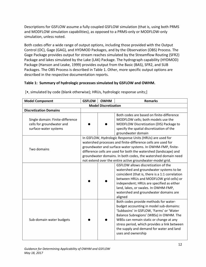
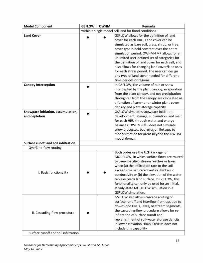
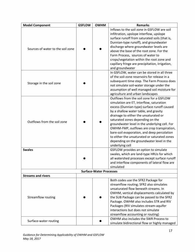
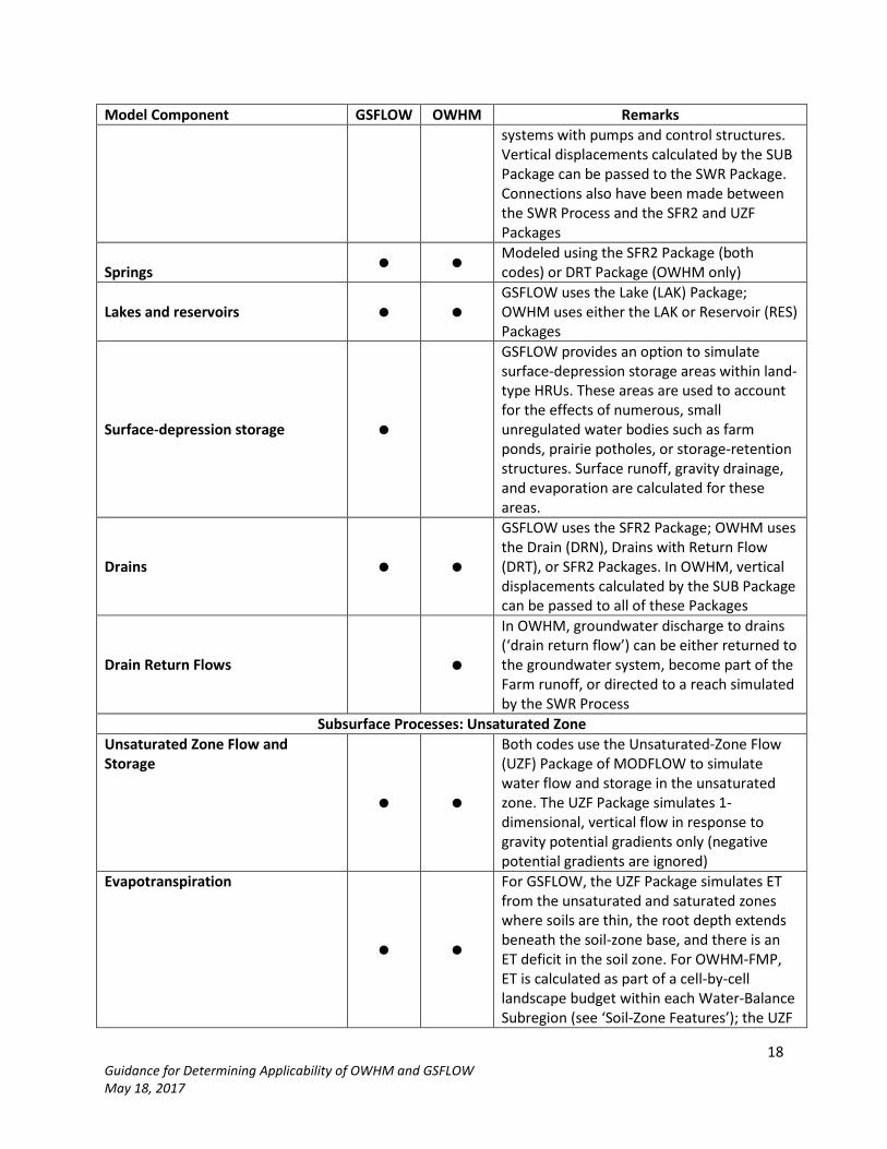
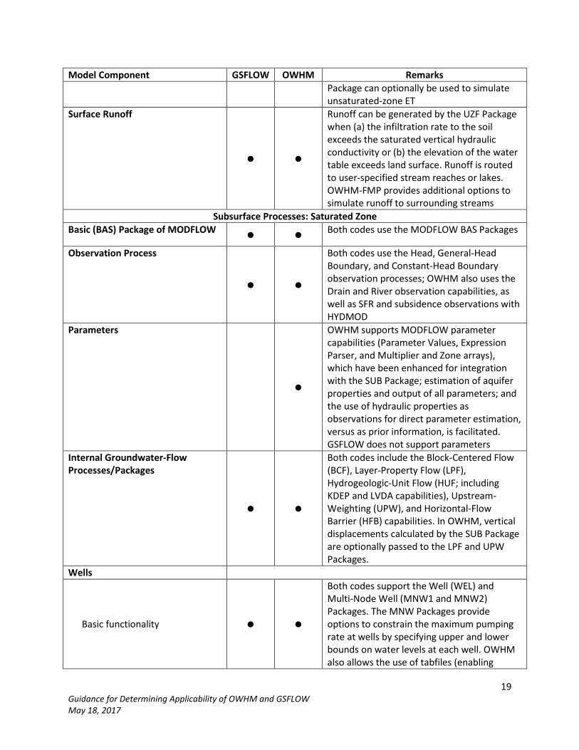
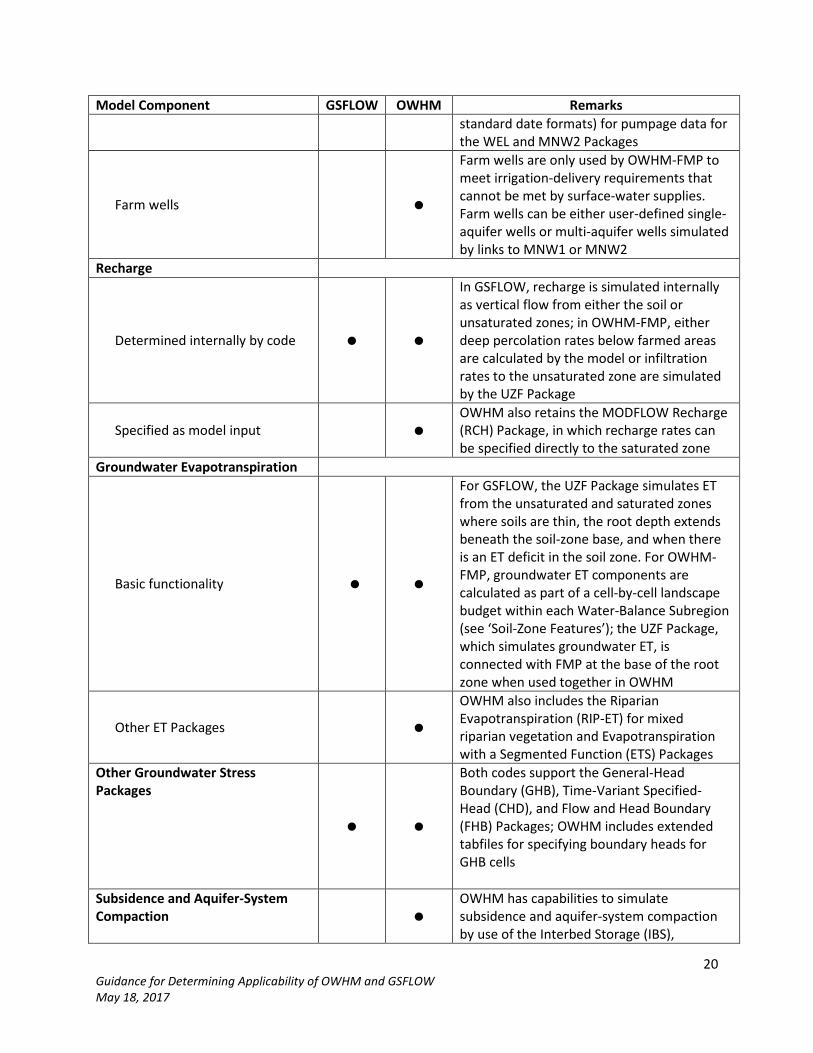
Table 1 provides a side-by-side synopsis of the hydrologic processes simulated by GSFLOW and OWHM. The table is arranged into five sections: Model Discretization, Watershed Processes, Surface-Water Processes, and Unsaturated and Saturated Zone Subsurface Processes. Commonalities and differences between the codes are noted. It is difficult to make direct comparisons for some of the hydrologic processes simulated by the two codes because of the different conceptualizations used in the development of each code. This is particularly true for the entries related to evapotranspiration, surface runoff and infiltration, and soil-zone features. In those cases, separate entries and descriptions of the different conceptualizations are provided.


Descriptions for GSFLOW assume a fully coupled GSFLOW simulation (that is, using both PRMS and MODFLOW simulation capabilities), as opposed to a PRMS-only or MODFLOW-only simulation, unless noted.

Both codes offer a wide range of output options, including those provided with the Output Control (OC), Gage (GAG), and HYDMOD Packages, and by the Observation (OBS) Process. The Gage Package provides output for stream reaches simulated by the Streamflow Routing (SFR2) Package and lakes simulated by the Lake (LAK) Package. The hydrograph capability (HYDMOD) Package (Hanson and Leake, 1999) provides output from the Basic (BAS), SFR2, and SUB Packages. The OBS Process is described in Table 1. Other, more specific output options are described in the respective documentation reports.

Table 1: Summary of hydrologic processes simulated by GSFLOW and OWHM.

[•, simulated by code (blank otherwise); HRUs, hydrologic response units;]

Model Component GSFLOW OWHM Remarks Model Discretization

Discretization Domains

Single domain: Finite-difference cells for groundwater and surface-water systems

• •

Both codes are based on finite-difference MODFLOW cells; both models use the MODFLOW Discretization (DIS) Package to specify the spatial discretization of the groundwater domain

Two domains

In GSFLOW, Hydrologic Response Units (HRUs) are used for watershed processes and finite-difference cells are used for groundwater and surface-water systems. In OWHM-FMP, finite-difference cells are used for both the watershed (landscape) and groundwater domains. In both codes, the watershed domain need not extend over the entire active groundwater-model grid.

• •

GSFLOW allows discretization of the watershed and groundwater systems to be coincident (that is, there is a 1:1 correlation between HRUs and MODFLOW grid cells) or independent; HRUs are specified as either land, lakes, or swales. In OWHM-FMP, watershed and groundwater domains are aligned

Sub-domain water budgets • •

Both codes provide methods for water-budget accounting in model sub-domains: ‘Subbasins’ in GSFLOW, ‘Farms’ or ‘Water Balance Subregions’ (WBSs) in OWHM. The WBSs can remain static or change at any stress period, which provides a link between the supply and demand for water and land uses and ownership


Model Component GSFLOW OWHM Remarks MODFLOW Grid Refinement

Globally refined or variably spaced • • Traditional approaches for grid refinement

Local Grid Refinement (LGR and associated Boundary Flow and Head, BFH, Packages)

• OWHM includes the MODFLOW-LGR capability, including simulation of Farm processes for both parent and child models

Time Discretization MODFLOW time-step and stress-period concepts

• •

Both codes use MODFLOW’s concept of time steps and stress periods. In GSFLOW, daily time steps are used; in OWHM, time steps can be of variable length, but the Farm Process requires time steps to be a minimum of several days (in practice, time steps are typically 14 days). OWHM also has sub-time-stepping within the Surface-Water Routing (SWR1) Package

Watershed Processes Climate Data and Climate-Distribution Methods

Climate data are needed to drive many of the hydrologic processes simulated by the two codes. Climate data are either read into or calculated internally by the two codes. GSFLOW has several options to distribute climate data within the model domain. These options include climate data that are (1) pre-distributed by the user to each HRU, (2) read as a constant value for all HRUs, or (3) distributed to each HRU by internal algorithms on the basis of the elevations of each HRU and those of the available weather stations, distance of each weather station from each HRU, and, optionally, latitude and longitude or each HRU and weather station. In OWHM-FMP, climate data are either pre-distributed to the cells within the model domain for all time or by stress periods, are represented as a time series for the entire model grid, or are read as a constant value for all cells within the model domain

Precipitation as rain • •

Daily precipitation rates are specified for GSFLOW; in OWHM-FMP, precipitation rates are constant over a stress period or are entered as a time series of daily (or other time step) values that are summed for each time step

Precipitation as snow or mixture of rain and snow •

Form of precipitation is determined by GSFLOW on the basis of daily air temperatures; OWHM-FMP does not simulate snow processes, but relies on linkages to models that do for areas beyond the OWHM model domain

Air temperature • • Daily maximum and minimum air temperatures specified for GSFLOW; in OWHM-FMP, maximum and minimum air


Model Component GSFLOW OWHM Remarks temperatures can be entered as a time series of daily (or other) values that are summed for each time step, or, if not specified directly, are part of the reference ET

Solar radiation •

Daily values of shortwave solar radiation can be either specified or calculated internally by GSFLOW; not specified directly for OWHM-FMP but are part of the reference ET

Evapotranspiration (ET) GSFLOW and OWHM-FMP use different terminology to refer to ET processes; therefore, these processes are differentiated below by code

i. Potential ET (PET) •

GSFLOW has six options to calculate PET internally, including the Jensen-Haise, Hamon, Hargreaves-Samani, Penman-Monteith, Priestley-Taylor, and pan-evaporation formulations. A seventh option is to input pre-distributed daily values of PET to each HRU

ii. Reference and Potential Crop ET •

In OWHM-FMP, reference ET is calculated prior to a simulation (such as by the Hargreaves-Samani, Priestley-Taylor, or Penman-Monteith formulations) and specified in the model input; potential crop ET, which is used to determine actual crop ET, can be either specified as a flux rate for each crop type or calculated internally by multiplying specified reference ET rates by user-specified crop coefficients

Actual ET Both codes simulate actual ET, but use different conceptualizations of the ET process. In GSFLOW, actual ET is simulated through canopy evaporation; snow sublimation; evaporation from surface depressions and impermeable surfaces; ET from the soil, saturated, and unsaturated zones; and by evaporation from lakes and streams. Soil ET is based on soil type (sand, silt, or clay) and cover type (bare soil, grass, shrub, or tree). OWHM-FMP also includes several ET components. ET from consumptive use is composed of crop-transpiratory and bare-soil evaporative components from three sources: groundwater, precipitation, and applied irrigation water. ET also can occur from the saturated and unsaturated zones and by evaporation from lakes and streams. The ET components in OWHM-Farm are further adjusted by areal fractions of transpiration and evaporation that represent sub-grid canopy and non-vegetation land use and by root uptake pressures. Positive pressures for ET under flooded conditions (such as riparian vegetation or rice) can be simulated, as can anoxia. Through the Riparian (RIP) ET Package, OWHM-FMP also can model ET for multiple riparian plant types


Model Component GSFLOW OWHM Remarks within a single model cell, and for flood conditions

Land Cover • • GSFLOW allows for the definition of land cover for each HRU. Land cover can be simulated as bare soil, grass, shrub, or tree; cover type is held constant over the entire simulation period. OWHM-FMP allows for an unlimited user-defined set of categories for the definition of land cover for each cell, and also allows for changing land cover/land uses for each stress period. The user can design any type of land cover needed for different time periods or regions

Canopy Interception • In GSFLOW, the volume of rain or snow

intercepted by the plant canopy, evaporation from the plant canopy, and net precipitation throughfall from the canopy are calculated as a function of summer or winter plant-cover density and plant-storage capacity

Snowpack initiation, accumulation, and depletion •

GSFLOW simulates snowpack initiation, development, storage, sublimation, and melt for each HRU through water and energy balances; OWHM-FMP does not simulate snow processes, but relies on linkages to models that do for areas beyond the OWHM model domain

Surface runoff and soil infiltration Overland-flow routing

i. Basic functionality • •

Both codes use the UZF Package for MODFLOW, in which surface flows are routed to user-specified stream reaches or lakes when (a) the infiltration rate to the soil exceeds the saturated vertical hydraulic conductivity or (b) the elevation of the water table exceeds land surface. In GSFLOW, this functionality can only be used for an initial, steady-state MODFLOW simulation in a GSFLOW simulation.

ii. Cascading-flow procedure •

GSFLOW also allows cascade routing of surface runoff and interflow from upslope to downslope HRUs, lakes, or stream segments; the cascading-flow procedure allows for re-infiltration of surface runoff and replenishment of soil-water storage deficits in lower-elevation HRUs; OWHM does not include this capability

Surface runoff and soil infiltration


Model Component GSFLOW OWHM Remarks GSFLOW: Both infiltration-excess (Hortonian) and saturation-excess (Dunnian) surface-runoff processes are simulated. Precipitation throughfall (that is, precipitation that exceeds the available canopy storage capacity), snowmelt, and cascading Hortonian upslope surface runoff are partitioned to the pervious, impervious, surface-depression storage, and preferential-flow reservoir portions of each land HRU. Downslope runoff and evaporation are calculated for the impervious areas; downslope runoff and soil infiltration are calculated for the pervious areas on the basis of antecedent soil-moisture conditions and a variable-source-area concept of runoff. Surface runoff, gravity drainage to the unsaturated zone, and evaporation are calculated for surface-depression storage areas. OWHM-FMP: Inefficient losses of irrigation and precipitation in excess of consumptive use in farm areas are partitioned into runoff return flow and deep-percolation components. Runoff return flows are calculated separately for irrigation and precipitation as the product of the inefficient loss for each component (that is, excess precipitation and excess irrigation) multiplied by user-specified inefficient-loss coefficients (alternatively, these coefficients can be determined from land-surface slope). Runoff return flows are then directed to the simulated stream network. Deep percolation to either the unsaturated or saturated zones is then calculated as the remainder of the sum of excess irrigation and precipitation less the sum of calculated runoff and ET from the unsaturated and saturated zones; deep percolation may be limited by the vertical hydraulic conductivity of the unsaturated zone. In non-farm areas, runoff and deep percolation are simulated by the UZF Package (see ‘Basic Functionality’ above).

Soil-Zone or Root-Zone Features Conceptualizations: GSFLOW: In GSFLOW, the soil zone is conceptualized as extending from the ground surface to the base of the average rooting depth of the dominant vegetative type covering the soil surface. The soil zone is partitioned into three reservoirs that occupy the same space but represent different soil-water processes at different soil-water content thresholds: the capillary reservoir (from wilting point to field capacity), gravity reservoir (field capacity to soil saturation), and preferential-flow reservoir (that part of the gravity reservoir from which “fast” interflow occurs, such as macropores). Soil water is partitioned among the three reservoirs on the basis of coupled continuity equations among the three reservoirs that are a function of soil and vegetation/crop characteristics, saturation status of the soil and unsaturated zone, availability of water to the soil, ET demand, and groundwater levels in the underlying MODFLOW cells. OWHM-FMP: In the Farm Process, the soil zone is conceptualized as extending from the ground surface to the base of the combined thickness of the root zone and capillary fringe. A total of six ET processes can occur within the soil zone or from the land surface overlying the soil zone: root-zone uptake by transpiration of precipitation (Tp), irrigation (Ti), and groundwater (Tgw) within the soil zone, as well as evaporation of groundwater (Egw) if the groundwater level is above the base of the capillary fringe. Bare-soil evaporation of precipitation (Ep) and irrigation (Ei) can occur from the land surface. The transpiratory and evaporative fractions of total potential crop ET are defined by crop coefficients specified as part of the model input. Options also are provided to reduce transpiration rates within the active root zone caused by stresses from anoxia and wilting. The soil-zone processes are based on an assumption of no soil-water storage changes within the root zone or capillary fringe based on simulations of variably saturated flow in soil columns reported by Schmid (2004) and Schmid and others (2006). OWHM also allows for properties such as the root depths to vary each stress period


Model Component GSFLOW OWHM Remarks

Sources of water to the soil zone • •

Inflows to the soil zone in GSFLOW are soil infiltration, upslope interflow, upslope surface runoff from saturated soils (that is, Dunnian-type runoff), and groundwater discharge where groundwater levels are above the base of the root zone. For the Farm Process, sources of water to crops/vegetation within the root zone and capillary fringe are precipitation, irrigation, and groundwater

Storage in the soil zone •

In GSFLOW, water can be stored in all three of the soil-zone reservoirs for release in a subsequent time step. The Farm Process does not simulate soil-water storage under the assumption of well managed soil moisture for agriculture and urban landscapes

Outflows from the soil zone • •

Outflows from the soil zone for a GSFLOW simulation are ET, interflow, saturation excess (Dunnian-type) surface runoff caused by a shallow water table, and gravity drainage to either the unsaturated or saturated zones depending on the groundwater level in the underlying cell. For OWHM-FMP, outflows are crop transpiration, bare-soil evaporation, and deep percolation to either the unsaturated or saturated zones depending on the groundwater level in the underlying cell

Swales

•

GSFLOW provides an option to simulate swales, which are land-type HRUs for which all watershed processes except surface runoff and interflow components of lateral flow are simulated

Surface-Water Processes Streams and rivers

Streamflow routing • •

Both codes use the SFR2 Package for streamflow routing; SFR2 also simulates unsaturated flow beneath streams. In OWHM, vertical displacements calculated by the SUB Package can be passed to the SFR2 Package. OWHM also includes STR and RIV Packages (RIV simulates stream-aquifer interactions but does not simulate streamflow accounting or routing)

Surface-water routing • OWHM also includes the SWR Process to simulate bidirectional flow or highly managed


Model Component GSFLOW OWHM Remarks systems with pumps and control structures. Vertical displacements calculated by the SUB Package can be passed to the SWR Package. Connections also have been made between the SWR Process and the SFR2 and UZF Packages

Springs • • Modeled using the SFR2 Package (both codes) or DRT Package (OWHM only)

Lakes and reservoirs • • GSFLOW uses the Lake (LAK) Package; OWHM uses either the LAK or Reservoir (RES) Packages

Surface-depression storage •

GSFLOW provides an option to simulate surface-depression storage areas within land-type HRUs. These areas are used to account for the effects of numerous, small unregulated water bodies such as farm ponds, prairie potholes, or storage-retention structures. Surface runoff, gravity drainage, and evaporation are calculated for these areas.

Drains • •

GSFLOW uses the SFR2 Package; OWHM uses the Drain (DRN), Drains with Return Flow (DRT), or SFR2 Packages. In OWHM, vertical displacements calculated by the SUB Package can be passed to all of these Packages

Drain Return Flows •

In OWHM, groundwater discharge to drains (‘drain return flow’) can be either returned to the groundwater system, become part of the Farm runoff, or directed to a reach simulated by the SWR Process

Subsurface Processes: Unsaturated Zone Unsaturated Zone Flow and Storage

• •

Both codes use the Unsaturated-Zone Flow (UZF) Package of MODFLOW to simulate water flow and storage in the unsaturated zone. The UZF Package simulates 1-dimensional, vertical flow in response to gravity potential gradients only (negative potential gradients are ignored)

Evapotranspiration

• •

For GSFLOW, the UZF Package simulates ET from the unsaturated and saturated zones where soils are thin, the root depth extends beneath the soil-zone base, and there is an ET deficit in the soil zone. For OWHM-FMP, ET is calculated as part of a cell-by-cell landscape budget within each Water-Balance Subregion (see ‘Soil-Zone Features’); the UZF


Model Component GSFLOW OWHM Remarks Package can optionally be used to simulate unsaturated-zone ET

Surface Runoff

• •

Runoff can be generated by the UZF Package when (a) the infiltration rate to the soil exceeds the saturated vertical hydraulic conductivity or (b) the elevation of the water table exceeds land surface. Runoff is routed to user-specified stream reaches or lakes. OWHM-FMP provides additional options to simulate runoff to surrounding streams

Subsurface Processes: Saturated Zone Basic (BAS) Package of MODFLOW • •

Both codes use the MODFLOW BAS Packages

Observation Process

• •

Both codes use the Head, General-Head Boundary, and Constant-Head Boundary observation processes; OWHM also uses the Drain and River observation capabilities, as well as SFR and subsidence observations with HYDMOD

Parameters

•

OWHM supports MODFLOW parameter capabilities (Parameter Values, Expression Parser, and Multiplier and Zone arrays), which have been enhanced for integration with the SUB Package; estimation of aquifer properties and output of all parameters; and the use of hydraulic properties as observations for direct parameter estimation, versus as prior information, is facilitated. GSFLOW does not support parameters

Internal Groundwater-Flow Processes/Packages

• •

Both codes include the Block-Centered Flow (BCF), Layer-Property Flow (LPF), Hydrogeologic-Unit Flow (HUF; including KDEP and LVDA capabilities), Upstream-Weighting (UPW), and Horizontal-Flow Barrier (HFB) capabilities. In OWHM, vertical displacements calculated by the SUB Package are optionally passed to the LPF and UPW Packages.

Wells

Basic functionality • •

Both codes support the Well (WEL) and Multi-Node Well (MNW1 and MNW2) Packages. The MNW Packages provide options to constrain the maximum pumping rate at wells by specifying upper and lower bounds on water levels at each well. OWHM also allows the use of tabfiles (enabling


Model Component GSFLOW OWHM Remarks standard date formats) for pumpage data for the WEL and MNW2 Packages

Farm wells •

Farm wells are only used by OWHM-FMP to meet irrigation-delivery requirements that cannot be met by surface-water supplies. Farm wells can be either user-defined single-aquifer wells or multi-aquifer wells simulated by links to MNW1 or MNW2

Recharge

Determined internally by code • •

In GSFLOW, recharge is simulated internally as vertical flow from either the soil or unsaturated zones; in OWHM-FMP, either deep percolation rates below farmed areas are calculated by the model or infiltration rates to the unsaturated zone are simulated by the UZF Package

Specified as model input • OWHM also retains the MODFLOW Recharge (RCH) Package, in which recharge rates can be specified directly to the saturated zone

Groundwater Evapotranspiration

Basic functionality • •

For GSFLOW, the UZF Package simulates ET from the unsaturated and saturated zones where soils are thin, the root depth extends beneath the soil-zone base, and when there is an ET deficit in the soil zone. For OWHM-FMP, groundwater ET components are calculated as part of a cell-by-cell landscape budget within each Water-Balance Subregion (see ‘Soil-Zone Features’); the UZF Package, which simulates groundwater ET, is connected with FMP at the base of the root zone when used together in OWHM

Other ET Packages • OWHM also includes the Riparian Evapotranspiration (RIP-ET) for mixed riparian vegetation and Evapotranspiration with a Segmented Function (ETS) Packages

Other Groundwater Stress Packages

• •

Both codes support the General-Head Boundary (GHB), Time-Variant Specified-Head (CHD), and Flow and Head Boundary (FHB) Packages; OWHM includes extended tabfiles for specifying boundary heads for GHB cells

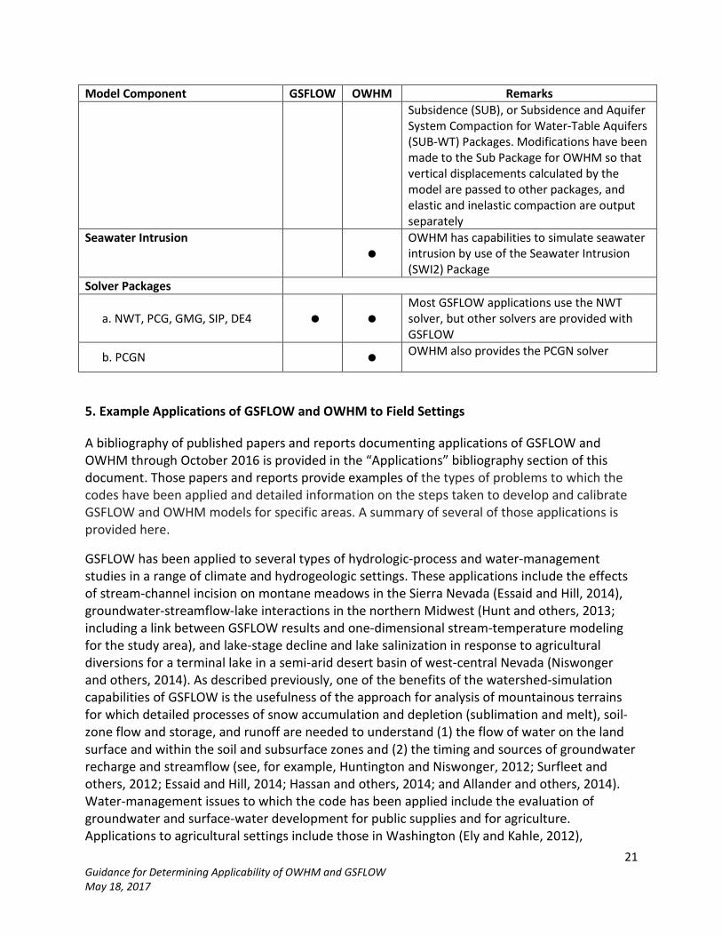
Subsidence and Aquifer-System Compaction •

OWHM has capabilities to simulate subsidence and aquifer-system compaction by use of the Interbed Storage (IBS),


Model Component GSFLOW OWHM Remarks Subsidence (SUB), or Subsidence and Aquifer System Compaction for Water-Table Aquifers (SUB-WT) Packages. Modifications have been made to the Sub Package for OWHM so that vertical displacements calculated by the model are passed to other packages, and elastic and inelastic compaction are output separately

Seawater Intrusion •

OWHM has capabilities to simulate seawater intrusion by use of the Seawater Intrusion (SWI2) Package

Solver Packages

a. NWT, PCG, GMG, SIP, DE4 • • Most GSFLOW applications use the NWT solver, but other solvers are provided with GSFLOW

b. PCGN • OWHM also provides the PCGN solver

5. Example Applications of GSFLOW and OWHM to Field Settings

A bibliography of published papers and reports documenting applications of GSFLOW and OWHM through October 2016 is provided in the “Applications” bibliography section of this document. Those papers and reports provide examples of the types of problems to which the codes have been applied and detailed information on the steps taken to develop and calibrate GSFLOW and OWHM models for specific areas. A summary of several of those applications is provided here.

GSFLOW has been applied to several types of hydrologic-process and water-management studies in a range of climate and hydrogeologic settings. These applications include the effects of stream-channel incision on montane meadows in the Sierra Nevada (Essaid and Hill, 2014), groundwater-streamflow-lake interactions in the northern Midwest (Hunt and others, 2013; including a link between GSFLOW results and one-dimensional stream-temperature modeling for the study area), and lake-stage decline and lake salinization in response to agricultural diversions for a terminal lake in a semi-arid desert basin of west-central Nevada (Niswonger and others, 2014). As described previously, one of the benefits of the watershed-simulation capabilities of GSFLOW is the usefulness of the approach for analysis of mountainous terrains for which detailed processes of snow accumulation and depletion (sublimation and melt), soil-zone flow and storage, and runoff are needed to understand (1) the flow of water on the land surface and within the soil and subsurface zones and (2) the timing and sources of groundwater recharge and streamflow (see, for example, Huntington and Niswonger, 2012; Surfleet and others, 2012; Essaid and Hill, 2014; Hassan and others, 2014; and Allander and others, 2014). Water-management issues to which the code has been applied include the evaluation of groundwater and surface-water development for public supplies and for agriculture. Applications to agricultural settings include those in Washington (Ely and Kahle, 2012),


California (Woolfenden and Nishikawa, 2014), Nevada (Niswonger and others, 2014), and northwest China (Wu and others 2014, 2015a,b; Tian and others, 2015a,b and 2016).

The primary purpose of the applications of either OWHM or the Farm Process has been to evaluate water-management alternatives, including conjunctive use of groundwater and surface-water supplies, in agricultural areas; specifically, the estimation of irrigation demands, surface-water and groundwater deliveries to meet these demands, and residual irrigation runoff and deep percolation. Several applications have been made to agricultural basins of California where groundwater withdrawals are typically unmetered; in these cases, the Farm Process was used to estimate groundwater pumping for irrigation (Faunt, 2009; Traum and others, 2014; Phillips and others, 2015; Hanson and others, 2014b,c; Hanson and others, 2015; Faunt and others, 2015). These include applications in arid to semi-arid settings where natural rates of runoff and snowmelt are small or nonexistent. In some applications (Hanson and others, 2012; Faunt and others, 2015; Hanson and others, 2015), runoff and groundwater-inflow rates from mountainous areas adjacent to the model domains have been estimated separately by use of a regional-scale precipitation-runoff model; those rates were specified along the boundaries of the OWHM-FMP model. OWHM and the Farm Process have been used with the SUB subsidence Package of MODFLOW in two applications, the Central Valley (Faunt, 2009) and Cuyama Valley (Hanson and others, 2015) models. Some of the advanced water-allocation capabilities provided by the Farm Process are described by Schmid and Hanson (2007) and applied to water-management conditions in the Pajaro Valley, California, by Hanson and others (2014b,c). Schmid and Hanson (2007) describe the application of the Farm Process to a prior-appropriation water-rights system for a hypothetical agricultural system having multiple farms with both surface-water and groundwater sources. Hanson and others (2014b,c) demonstrate the simulation of a coastal water-supply distribution system that is used to replace coastal groundwater pumping. The system consists of alternative sources of supplemental water from a managed aquifer recharge and recovery system, a wastewater-recycle facility, and remotely placed supplemental wells. OWHM also is being used as part of research studies of hypothetical agricultural systems to develop crop-optimization and related water-allocation schemes (Fowler and others, 2015, 2016).

Both codes have been used to evaluate the effects of climate change and climate extremes on hydrologic and anthropogenic water-resource systems. Applications of GSFLOW to the evaluation of climate change have been made to snow-dominated mountainous regions in the Sierra Nevada (Huntington and Niswonger, 2012; Albano and others, 2015); mixed rain-snow precipitation climate in the Cascade Range in Oregon (Surfleet and Tullos, 2012); and a lake-dominated system in the north-temperature regime of north-central Wisconsin (Hunt and others, 2013). OWHM-FMP Process was applied to the evaluation of conjunctive management of surface-water and groundwater supplies in the Central Valley of California by Hanson and others (2012) and to the potential effects on project operations on the Lower Rio Grande (U.S. Bureau of Reclamation, 2016). Projections of future water availability under historical climate conditions similar to the recent past also have been made using both codes (GSFLOW by Niswonger and others, 2014; OWH-Farm by Hanson and others, 2014b,c; Hanson and others, 2015; Faunt and others, 2015).


6. Recommendations for Model Selection

Through the Farm Process, OWHM provides several specialized capabilities to represent and manage the surface-water and groundwater deliveries to farms that extend beyond the core water-withdrawal and irrigation-application capabilities of MODFLOW, MODFLOW-NWT, and GSFLOW. OWHM also provides options for simulating the effects of land subsidence on coupled groundwater and surface-water systems with irrigated agriculture. However, if these capabilities are not needed, the WMA recommends use of GSFLOW for most projects requiring hydrologic simulation and analysis of coupled groundwater/surface-water/watershed systems.

7. Bibliography

A. Documentation for each Code

GSFLOW

Henson, W.R., Medina, R.L., Mayers, C.J., Niswonger, R.G., and Regan, R.S., 2013, CRT—Cascade routing tool to define and visualize flow paths for grid-based watershed models: U.S. Geological Survey Techniques and Methods, book 6, chap. D2, 28 p., http://pubs.usgs.gov/tm/tm6d2/.

Markstrom, S.L., Niswonger, R.G., Regan, R.S., Prudic, D.E., and Barlow, P.M., 2008, GSFLOW—Coupled ground-water and surface-water flow model based on the integration of the Precipitation-Runoff Modeling System (PRMS) and the modular ground-water flow model (MODFLOW-2005): U.S. Geological Survey Techniques and Methods 6-D1, 240 p.

Markstrom, S.L., Regan, R.S., Hay, L.E., Viger, R.J., Webb, R.M.T., Payn, R.A., and LaFontaine, J.H., 2015, PRMS-IV, the precipitation-runoff modeling system, version 4: U.S. Geological Survey Techniques and Methods, book 6, chap. B7, 158 p., http://dx.doi.org/10.3133/tm6B7.

Regan, R.S., Niswonger, R.G., Markstrom, S.L., and Barlow, P.M., 2015, Documentation of a restart option for the U.S. Geological Survey coupled groundwater and surface-water flow (GSFLOW) model: U.S. Geological Survey Techniques and Methods, book 6, chap. D3, 19 p., http://dx.doi.org/10.3133/tm6D3/.

OWHM

Hanson, R.T., Boyce, S.E., Schmid, Wolfgang, Hughes, J.D., Mehl, S.M., Leake, S.A., Maddock, Thomas, III, and Niswonger, R.G., 2014a, One-Water Hydrologic Flow Model (MODFLOW-OWHM): U.S. Geological Survey Techniques and Methods 6–A51, 120 p., http://dx.doi.org/10.3133/tm6A51.

Maddock, Thomas, III, Baird, K.J., Hanson, R.T., Schmid, Wolfgang, and Ajami, Hoori, 2012, RIP-ET: A Riparian Evapotranspiration Package for MODFLOW-2005: U.S. Geological Survey Techniques and Methods 6-A39, 76 p., http://pubs.usgs.gov/tm/tm6a39/.

http://pubs.usgs.gov/tm/tm6d2/

http://dx.doi.org/10.3133/tm6B7

http://dx.doi.org/10.3133/tm6D3/

http://dx.doi.org/10.3133/tm6A51

http://pubs.usgs.gov/tm/tm6a39/


Schmid, Wolfgang, and Hanson R.T., 2009, The farm process version 2 (FMP2) for MODFLOW-2005—Modifications and upgrades to FMP1: U.S. Geological Survey Techniques in Water Resources Investigations, book 6, chap. A32, 102 p.

Schmid, W., Hanson, R.T., Maddock III, T.M., and Leake, S.A., 2006, User’s guide for the farm process (FMP) for the U.S. Geological Survey’s modular three-dimensional finite-difference ground-water flow model, MODFLOW-2000: U.S. Geological Survey Techniques and Methods 6–A17, 127 p.

B. Applications

A bibliography of published papers and reports documenting applications of GSFLOW and OWHM through October 2016 is provided below. The intent of the bibliographies is to provide a set of papers and reports that illustrate the types of problems to which the codes have been applied, and detailed information on the steps taken to develop and calibrate GSFLOW and OWHM (or Farm) models for specific areas. Additional criteria for including specific citations are that the publications are relatively easily accessible, have gone through an acceptable peer review system, and represent completed work (as opposed to an interim analysis). Conference and symposium papers often do not meet some or all of these criteria and, therefore, are not included in the bibliographies. Also, reports published by governmental agencies, engineering consulting firms, and universities can be difficult to obtain and often do not receive the level of peer review that is provided by a journal or the USGS reports-approval process. Although conference papers, consulting reports, and governmental reports have been written to describe applications of both codes, they are not included in the bibliography for these reasons.

GSFLOW

Albano, C.M., Dettinger, M.D., McCarthy, M.I., Welborn, T.L., and Cox, D.A., 2015, Use of a hypothetical winter-storm disaster scenario to identify vulnerabilities, mitigation options, and science needs in the greater Lake Tahoe, Reno, and Carson City region, USA: Natural Hazards, 79, 22 p., DOI 10.1007/s11069-015-2003-4. (This paper is an application of the GSFLOW model described by Huntington and Niswonger, 2012, to assess vulnerabilities, mitigation options, and science needs related to extreme winter storms and associated flood risks.)

Allander, K.K., Niswonger, R.G., and Jeton, A.E., 2014, Simulation of the Lower Walker River Basin hydrologic system, west-central Nevada, using PRMS and MODFLOW models: U.S. Geological Survey Scientific Investigations Report 2014-5190, 93 p. http://dx.doi.org/10.3133/sir20145190. (Companion report to Niswonger and others, 2014.)

Carroll, R. W., Huntington, J. L., Snyder, K. A., Niswonger, R., Morton, C., and Stringham, T. K., 2016, Evaluating mountain meadow groundwater response to Pinyonâ€�Juniper and temperature in a Great Basin watershed: Ecohydrology, http://dx.doi.org/10.1002/eco.1792

Doherty, John, and Hunt, R.J., 2009, Two statistics for evaluating parameter identifiability and error reduction: Journal of Hydrology, v. 366, p. 119-127. (Primary purpose of paper is the

http://dx.doi.org/10.3133/sir20145190

http://dx.doi.org/10.1002/eco.1792

http://dx.doi.org/10.1002/eco.1792


description and analysis of the two statistics with application to the Trout Lake Watershed, Wisconsin.)

Ely, D.M., and Kahle, S.C., 2012, Simulation of groundwater and surface-water resources and evaluation of water-management alternatives for the Chamokane Creek basin, Stevens County, Washington: U.S. Geological Survey Scientific Investigations Report 2012–5224, 74 p. http://pubs.er.usgs.gov/publication/sir20125224

Essaid, H.I., and Hill, B.R., 2014, Watershed-scale modeling of streamflow change in incised montane meadows: Water Resources Research, vol. 50, pp. 2657-2678, doi:10.1002/2013WR014420.

Fulton, J.W., Risser, D.W., Regan, R.S., Walker, J.F., Hunt, R.J., Niswonger, R.G., Hoffman, S.A., and Markstrom, S.L., 2015, Water-budgets and recharge-area simulations for the Spring Creek and Nittany Creek Basins and parts of the Spruce Creek Basin, Centre and Huntingdon Counties, Pennsylvania, Water Years 2000–06: U.S. Geological Survey Scientific Investigations Report 2015–5073, 86 p, http://dx.doi.org/10.3133/sir20155073.

Hassan, T. S. M., Lubczynski, M. W., Niswonger, R. G., and Su, Z. (2014). Surface-groundwater interactions in hard rocks in Sardon Catchment of western Spain: An integrated modeling approach: Journal of Hydrology, 517, 390-410. doi:10.1016/j.jhydrol.2014.05.026. http://www.sciencedirect.com/science/article/pii/S0022169414003904

Hunt, R.J., Walker, J.F., Selbig, W.R., Westenbroek, S.M., and Regan, R.S., 2013, Simulation of climate-change effects on streamflow, lake water budgets, and stream temperature using GSFLOW and SNTEMP, Trout Lake Watershed, Wisconsin: U.S. Geological Survey Scientific Investigations Report 2013–5159, 118 p. http://pubs.er.usgs.gov/publication/sir20135159

Hunt, R.J., Westenbroek, S.M., Walker, J.F., Selbig, W.R., Regan, R.S., Leaf, A.T., and Saad, D.A., 2016, Simulation of climate change effects on streamflow, groundwater, and stream temperature using GSFLOW and SNTEMP in the Black Earth Creek Watershed, Wisconsin: U.S. Geological Survey Scientific Investigations Report 2016-5091, 117 p., http://dx.doi.org/10.3133/sir20165091

Huntington, J.L., and Niswonger, R.G., 2012, Role of surface-water and groundwater interactions on projected summertime streamflow in snow dominated regions: An integrated modeling approach: Water Resources Research, v. 48, W11524, doi: 10.1029/2012WR012319.

Mejia, J.F., Huntington, Justin, Hatchett, Benjamin, Koracin, Darko, and Niswonger, R.G., 2012, Linking global climate models to an integrated hydrologic model: Using an individual station downscaling approach: Journal of Contemporary Water Research and Education, issue 147, p. 17-27.

Niswonger, R. G., Allander, K. K., and Jeton, A. E., 2014, Collaborative modelling and integrated decision support system analysis of a developed terminal lake basin: Journal of Hydrology, doi:

http://pubs.er.usgs.gov/publication/sir20125224


http://www.sciencedirect.com/science/article/pii/S0022169414003904


http://pubs.er.usgs.gov/publication/sir20135159




10.1016/j.jhydrol.2014.05.043, http://www.sciencedirect.com/science/article/pii/S0022169414004077

Surfleet, C.G. and Tullos, Desiree, 2012, Uncertainty in hydrologic modeling for estimating hydrologic response due to climate change (Santiam River, Oregon): Hydrological Processes, DOI: 10.1002/hyp.9485.

Surfleet, C.G., Tullos, Desiree, Chang, Heejun, and Jun, Il-Won, 2012, Selection of hydrologic modeling approaches for climate change assessment: A comparison of model scale and structures: Journal of Hydrology, v. 464–465, p. 233-248 http://dx.doi.org/10.1016/j.jhydrol.2012.07.012

Tian, Yong, Zheng, Yi, Wu, Bin, Wu, Xin, Liu, Jie, and Zheng, Chunmiao, 2015a, Modeling surface water-groundwater interaction in arid and semi-arid regions with intensive agriculture. Environmental Modelling & Software, 63, p. 170-184, http://dx.doi.org/10.1016/j.envsoft.2014.10.011.

Tian, Yong, Zheng, Yi, and Zheng, Chunmiao, 2016, Development of a visualization tool for integrated surface water-groundwater modeling: Computers and Geosciences, v. 86, p. 1-14, http://dx.doi.org/10.1016/j.cageo.2015.09.019 (This paper describes a graphical user interface for integrated hydrologic modeling and uses the GSFLOW model developed by Wu and others, 2014, to demonstrate the tool.)

Tian, Yong, Zheng, Yi, Zheng, Chunmiao, Xiao, Honglang, Fan, Wenjie, Zou, Songbing, Wu, Bin, Yao, Yingying, Zhang, Aijing, and Liu, Jie, 2015b, Exploring scale-dependent ecohydrological responses in a large endorheic river basin through integrated surface water-groundwater modeling: Water Resources Research, v. 51, p. 4065-4085, doi:10.1002/2015WR016881.

Woolfenden, L.R., and Nishikawa, Tracy, eds., 2014, Simulation of groundwater and surface-water resources of the Santa Rosa Plain watershed, Sonoma County, California: U.S. Geological Survey Scientific Investigations Report 2014-5052, 258 p., http://dx.doi.org/10.3133/sir20145052.

Wu, Bin, Zheng, Yi, Tian, Yong, Wu, Xin, Yao, Yingying, Han, Feng, Liu, Jie, and Zheng, Chunmiao, 2014, Systematic assessment of the uncertainty in integrated surface water-groundwater modeling based on the probabilistic collocation method: Water Resources Research, DOI: 10.1002/2014WR015366.

Wu, Bin, Zheng, Yi, Wu, Xin, Tian, Yong, Han, Feng, Liu, Jie, and Zheng, Chunmiao, 2015a, Optimizing water resources management in large river basins with integrated surface water-groundwater modeling: A surrogate-based approach: Water Resources Research, v. 51, p. 2153-2173, doi:10.1002/2014WR016653.

Wu, Xin, Zheng, Yi, Wu, Bin, Tian, Yong, Han, Feng, and Zheng, Chunmiao, 2015b, Optimizing conjunctive use of surface water and groundwater for irrigation to address human-nature



http://dx.doi.org/10.1016/j.jhydrol.2012.07.012

http://dx.doi.org/10.1016/j.envsoft.2014.10.011

http://dx.doi.org/10.1016/j.cageo.2015.09.019

http://pubs.usgs.gov/sir/2014/5052/

http://pubs.usgs.gov/sir/2014/5052/


water conflicts: A surrogate modeling approach: Agricultural Water Management, http://dx.doi.org/10.1016/j.agwat.2015.08.022.

OWHM or Farm

Boyce, S.E., Nishikawa, T., and Yeh, W.G., 2015, Reduced order modeling of the Newton formulation of MODFLOW to solve unconfined groundwater flow: Advances in Water Resources, 83, pp. 250-262. http://dx.doi.org/10.1016/j.advwatres.2015.06.005 (This paper describes a partially calibrated scoping model of Santa Barbara, CA, using OWHM; constructed to illustrate the model-reduction technique.)

Faunt, C.C., ed., 2009, Groundwater availability of the Central Valley Aquifer, California: U.S. Geological Survey Professional Paper 1766, 225 p.

Faunt, C.C., Stamos, C.L., Flint, L.E., Wright, M.T., Burgess, M.K., Sneed, Michelle, Brandt, Justin, Martin, Peter, and Coes, A.L., 2015, Hydrogeology, hydrologic effects of development, and simulation of groundwater flow in the Borrego Valley, San Diego County, California: U.S. Geological Survey Scientific Investigations Report 2015–5150, 136 p.

Fowler, K., R., Jenkins, E.W., Ostrove, C., Chrispell, J.C., Farthing, M.W., Parno, M., 2015, A decision making framework with MODFLOW-FMP2 via optimization: determining trade-offs in crop selection: Environmental Modelling and Software, v. 69, p. 280-291, http://www.sciencedirect.com/science/article/pii/S1364815214003624 (Demonstration of an optimization approach for crop management using one of the Farm version 2 hypothetical test cases.)

Fowler, K., R., Jenkins, E.W., Parno, M., Chrispell, J.C., Colon, A.I., and Hanson, R.T., 2016, Development and use of mathematical models and software frameworks for integrated analysis of agricultural systems and associated water use impacts: AIMS Agriculture and Food, v. 1, no. 2, p. 208-226, DOI: 10.3934/agrfood.2016.2.208. (Describes a framework for quantifying and evaluating the impact of water-policy decisions on regional agricultural systems and stakeholders using one of the Farm version 2 and OWHM hypothetical test cases.)

Hanson, R.T., Flint, L.E., Faunt, C.C., Gibbs, D.R., and Schmid, W., 2015, Hydrologic models and analysis of water availability in Cuyama Valley, California (ver. 1.1, May 2015): U.S. Geological Survey Scientific Investigations Report 2014–5150, 150 p., http://dx.doi.org/10.3133/sir20145150.

Hanson, R.T., Flint, L.E., Flint, A.L., Dettinger, M.D., Faunt, C.C., Cayan, D., and Schmid, Wolfgang, 2012, A method for physically based model analysis of conjunctive use in response to potential climate changes: Water Resources Research, v. 48, 23 p., doi:10.1029/2011WR010774

Hanson, R.T., Lockwood, B., and Schmid, Wolfgang, 2014b, Analysis of projected water availability with current basin management plan, Pajaro Valley, California: Journal of Hydrology, v. 519, p. 131–147.

http://dx.doi.org/10.1016/j.agwat.2015.08.022

http://dx.doi.org/10.1016/j.advwatres.2015.06.005



Hanson, R.T., Schmid, Wolfgang, Faunt, C.C., and Lockwood, B., 2010, Simulation and analysis of conjunctive use with MODFLOW’s Farm Process: Ground Water v. 48, no. 5, p. 674–689. (DOI: 10.1111/j.1745-6584.2010.00730.x) (Summary article of Farm capabilities using examples from the Pajaro and Central Valleys Farm models.)

Hanson, R.T., Schmid, Wolfgang, Faunt, C.C., Lear, Jonathan, Lockwood, B., and Harich, C., 2014c, Integrated hydrologic model of Pajaro Valley, Santa Cruz and Monterey Counties, California: U.S. Geological Survey Scientific Investigations Report 2014–5111, 166 p.

Liu, T. and Luo, Y., 2012, An empirical approach simulating evapotranspiration from groundwater under different soil water conditions: Journal of Environmental Earth Sciences, 11 p., doi 10.1007/s12665-012-1577-3. (This paper describes simulation of column experiments, not an actual field application.)

Phillips, S.P., Rewis, D.L., and Traum, J.A., 2015, Hydrologic model of the Modesto Region, California, 1960–2004: U.S. Geological Survey Scientific Investigations Report, 2015–5045, 69 p., http://dx.doi.org/10.3133/sir20155045.

Russo, T.A, Fisher, A.T., and Lockwood, B.S., 2014, Assessment of managed aquifer recharge site suitability using a GIS and modeling, Ground Water, v. 53, no. 3, p.1-12, doi: 10.1111/gwat.12213

Schmid, W., and Hanson, R.T., 2007, Simulation of intra- or trans-boundary water-rights hierarchies using the Farm Process for MODFLOW-2000: ASCE Journal of Water Resources Planning and Management, v. 133, no. 2, pp. 166-178 (DOI: 10.1061/(ASCE)0733-9496(2007)133:2(166))

Schmid, Wolfgang, Hanson, R.T., Hughes, J., Leake, S.A., and Niswonger, R., 2014, Feedback of land subsidence on the movement and conjunctive use of water resources: Environmental Modelling and Software, v. 62, p. 253-270, http://dx.doi.org/10.1016/j.envsoft.2014.08.006

Schmid, W., King, J.P., and Maddock III., T.M., 2009, Conjunctive surface-water/ground-water model in the Southern Rincon Valley using MODFLOW-2005 with the Farm Process: prepared for the Elephant Butte Irrigation District, Las Cruces, NM; New Mexico Water Resources Research Institute Completion Report No. 350.

Traum, J.A., Phillips, S.P., Bennett, G.L., Zamora, Celia, and Metzger, L.F., 2014, Documentation of a groundwater flow model (SJRRPGW) for the San Joaquin River Restoration Program study area, California: U.S. Geological Survey Scientific Investigations Report 2014–5148, 151 p., http://dx.doi.org/10.3133/sir20145148.

U.S. Bureau of Reclamation, 2016, Continued implementation of the 2008 operating agreement for the Rio Grande Project, draft Environmental Impact Statement, New Mexico and Texas: U.S. Bureau of Reclamation, Upper Colorado Region, 398 p. (last accessed October 27, 2016 at http://www.usbr.gov/uc/envdocs/eis/pdf/RGOA_DEIS_20160313_508.pdf)




8. References cited in the Guidance document that are not included in the Bibliography

Bakker, M., Schaars, F., Hughes, J.D., Langevin, C.D., Dausman, A.M., 2013, Documentation of the seawater intrusion (SWI2) package for MODFLOW: U.S. Geological Survey Techniques and Methods, book 6, chap. A46, 47 p.

Banta, E.R., 2000, MODFLOW-2000, the U.S. Geological Survey modular ground-water model -- Documentation of packages for simulating evapotranspiration with a segmented function (ETS1) and drains with returnflow (DRT1): U.S. Geological Survey Open-File Report 00-466, 127 p.

California Department of Water Resources, 2017, IWFM: Integrated Water Flow Model – Demand Calculator (IDC): Accessed on March 10, 2017, http://baydeltaoffice.water.ca.gov/modeling/hydrology/IDC/index_IDC.cfm.

Flint, A.L., and Flint, L.E., 2007, Application of the Basin Characterization Model to estimate in-place recharge and runoff potential in the Basin and Range carbonate-rock aquifer system, White Pine County, Nevada, and adjacent areas in Nevada and Utah: U.S. Geological Survey Scientific Investigations Report 2007–5099, 20 p, http://pubs.water.usgs.gov/sir20075099

Flint, A.L., Flint, L.E., Hevesi, J.A., and Blainey, J.M., 2004, Fundamental concepts of recharge in the Desert Southwest, a regional modeling perspective, in Hogan, J.F., Phillips, F.M., and Scanlon, B.R., eds., Groundwater recharge in a desert environment, the Southwestern United States: American Geophysical Union, Water Science and Applications Series, v. 9, p. 159–184.

Halford, K.J., and Hanson, R.T., 2002, User guide for the Drawdown-Limited, Multi-Node Well (MNW) Package for the U.S. Geological Survey's modular three-dimensional finite-difference ground-water flow model, version MODFLOW-96 and MODFLOW-2000: U.S. Geological Survey Open-File Report 02-293, 33 p.

Hanson, R.T., and Leake, S.A., 1999, Documentation for HYDMOD, a program for extracting and processing time-series data from the U.S. Geological Survey’s modular three-dimensional finite-difference ground-water flow model: U.S. Geological Survey Open-File Report 98-564, 57 p.

Harbaugh, A.W., 2005, MODFLOW-2005, the U.S. Geological Survey modularground-water model--the ground-water flow process: U.S. Geological Survey Techniques and Methods 6 A-16, 9 ch.

Harter, Thomas, and Morel-Seytoux, Hubert, 2013, Peer review of the IWFM, MODFLOW and HGS Model Codes: Potential for water management applications in California’s Central Valley and other irrigated groundwater basins: Final Report, California Water and Environmental Modeling Forum, 112 p., Sacramento, California, http://www.cwemf.org/Pubs/index.htm.

Healy, R.W., 2010, Estimating groundwater recharge: Cambridge, United Kingdom, Cambridge University Press, 245 p.

http://baydeltaoffice.water.ca.gov/modeling/hydrology/IDC/index_IDC.cfm

http://pubs.water.usgs.gov/sir20075099

http://www.cwemf.org/Pubs/index.htm


Hoffmann, J., Leake, S.A., Galloway, D.L., and Wilson, A.M., 2003, MODFLOW-2000 Ground-Water Model--User Guide to the Subsidence and Aquifer-System Compaction (SUB) Package: U.S. Geological Survey Open-File Report 03-233, 44 p.

Hughes, J.D., Langevin, C.D., Chartier, K.L., and White, J.T., 2012, Documentation of the Surface-Water Routing (SWR1) Process for modeling surface-water flow with the U.S. Geological Survey Modular Ground-Water Model (MODFLOW-2005): U.S. Geological Survey Techniques and Methods, book 6, chap. A40 (Version 1.0), 113 p.

Konikow, L.F., Hornberger, G.Z., Halford, K.J., and Hanson, R.T., 2009, Revised multi-node well (MNW2) package for MODFLOW ground-water flow model: U.S. Geological Survey Techniques and Methods 6-A30, 67 p.

Leake, S.A. and Galloway, D.L., 2007, MODFLOW ground-water model – User guide to the Subsidence and Aquifer-System Compaction Package (SUB-WT) for water-table aquifers: U.S. Geological Survey Techniques and Methods 6-A23, 42 p.

Leake, S.A. and Prudic, D.E., 1991, Documentation of a computer program to simulate aquifer-system compaction using the modular finite-difference ground-water flow model: U.S. Geological Survey Techniques of Water-Resources Investigations, Book 6, Chapter A2, 68 p.

Mehl, S.W. and Hill, M.C., 2007, MODFLOW-2005, the U.S. Geological Survey modular ground-water model -- documentation of the multiple-refined-areas capability of local grid refinement (LGR) and the Boundary Flow and Head (BFH) Package: U.S. Geological Survey Techniques and Methods 6-A21. 13 p.

Mehl, S.W., and Hill, M.C., 2013, MODFLOW-LGR -- Documentation of ghost node local grid refinement (LGR2) for multiple areas and the boundary flow and head (BFH2) package: U.S. Geological Survey Techniques and Methods 6-A44, 43 p.

Merritt, M.L., and Konikow, L.F., 2000, Documentation of a computer program to simulate lake-aquifer interaction using the MODFLOW ground-water flow model and the MOC3D solute transport model: Water-Resources Investigations Report 00-4167, 146 p.

Niswonger, R.G., Panday, Sorab, and Ibaraki, Motomu, 2011, MODFLOW-NWT, A Newton formulation for MODFLOW-2005: U.S. Geological Survey Techniques and Methods 6-A37, 44 p.

Niswonger, R.G. and Prudic, D.E., 2005, Documentation of the Streamflow-Routing (SFR2) Package to include unsaturated flow beneath streams--A modification to SFR1: U.S. Geological Survey Techniques and Methods, Book 6, Chap. A13, 47 p.

Niswonger, R.G., Prudic, D.E., and Regan, R.S., 2006, Documentation of the Unsaturated-Zone Flow (UZF1) Package for modeling unsaturated flow between the land surface and the water table with MODFLOW-2005: U.S. Geological Survey Techniques and Methods, book 6, chap. A19, 74 p.


Prudic, D.E., 1989, Documentation of a computer program to simulate stream-aquifer relations using a modular, finite-difference, ground-water flow model: U.S. Geological Survey Open-File Report 88-729, 113 p.

Prudic, D.E., Konikow, L.F., and Banta, E.A., 2004, A new Streamflow-Routing (SFR1) Package to simulate stream-aquifer interaction with MODFLOW-2000: U.S. Geological Survey Open-File Report 04-1042, 95 p.

Scanlon, B.R., Healy, R. W., and Cook, P.G., 2002, Choosing appropriate techniques for quantifying groundwater recharge: Hydrogeology Journal, v. 10, p. 18-39.

Schmid, Wolfgang, 2004, A Farm Package for MODFLOW-2000: Simulation of irrigation demand and conjunctively managed surface-water and ground-water supply: PhD Dissertation, Department of Hydrology and Water Resources, The University of Arizona, 278 p.

Stanton, J.S., Qi, S.L., Ryter, D.W., Falk, S.E., Houston, N.A., Peterson, S.M., Westenbroek, S.M., and Christenson, S.C., 2011, Selected approaches to estimate water-budget components of the High Plains, 1940 through 1949 and 2000 through 2009: U.S. Geological Survey Scientific Investigations Report 2011–5183, 79 p.

guidance for determining applicability ... - water … include advanced capabilities for simulation...

Documents