handbook on radio astronomy - itu.int · - iii - radio astronomy introduction introduction to the...
TRANSCRIPT

HANDBOOK ON RADIO ASTRONOMY
Printed in Switzerland Geneva, 2013
ISBN: 978-92-61-14481-4 Photo credit: ATCA David Smyth
International Telecommunication Union
Sales and Marketing Division Place des Nations CH-1211 Geneva 20 Switzerland Fax: +41 22 730 5194 Tel.: +41 22 730 6141 E-mail: [email protected] Web: www.itu.int/publications
E d i t i o n o f 2 0 1 3Radiocommunication Bureau
*38650*
HANDBOOK ON RADIO ASTRONOMY
Edition of 2013

Handbook on
Radio Astronomy Third Edition
EDITION OF 2013
RADIOCOMMUNICATION BUREAU
Cover photo: Six identical 22-m antennas make up CSIRO's Australia Telescope Compact Array, an earth-rotation synthesis telescope located at the Paul Wild Observatory.
Credit: David Smyth.
ITU 2013
All rights reserved. No part of this publication may be reproduced, by any means whatsoever, without the prior written permission of ITU.
- iii -
Radio Astronomy Introduction
Introduction to the third edition by
the Chairman of ITU-R Working Party 7D
(Radio Astronomy)
It is an honour and privilege to present the third edition of the Handbook – Radio Astronomy, and I do so
with great pleasure.
The Handbook is not intended as a source book on radio astronomy, but is concerned principally with those
aspects of radio astronomy that are relevant to frequency coordination, that is, the management of radio
spectrum usage in order to minimize interference between radiocommunication services. Radio astronomy
does not involve the transmission of radiowaves in the frequency bands allocated for its operation, and
cannot cause harmful interference to other services. On the other hand, the received cosmic signals are
usually extremely weak, and transmissions of other services can interfere with such signals.
In twelve chapters and five Appendices, the Handbook introduces the reader to radio astronomy viewed as a
radiocommunication service for the purpose of frequency coordination. It starts with a preamble on radio
astronomy and society, outlining the role and benefits of radio astronomy to society, often extending beyond
astronomy. The Handbook then covers areas such as the characteristics of radio astronomy, preferred
frequency bands for observations, special radio astronomy applications, vulnerability to radio frequency
interference (RFI) from other services, and issues associated with sharing the radio spectrum with other
services. Additional chapters have been included in this third edition of the Handbook on techniques for
mitigating the effects of RFI, on the establishment and characteristics of Radio Quiet Zones (RQZ), on the
searches for extraterrestrial intelligence (SETI) and on ground-based radar astronomy. New Appendices have
been added to explain the use of units and the dB scale in radio astronomy, and an extensive list of
acronyms.
Almost ten years have passed since the second edition of the Handbook – Radio Astronomy was published.
In the meantime ITU has held three World Radiocommunication Conferences (WRC-2003, WRC-2007 and
WRC-2012).
In this period, there has been a virtual explosion in the development of communication services, and wireless
services are now all pervasive in our multi-connected society. In parallel, technological developments in
radio astronomy have enabled observations over very wide frequency bands, often not covered by the ITU
allocations. Such developments present a challenge for the protection of radio astronomy and new methods
had to be explored. New techniques on RFI mitigation are under continuous development, and RQZ have
been defined to provide unique places on the planet where radio astronomy can proceed with minimal
interference. Such developments have been covered within ITU with new and extensive ITU-R Reports.
Radio astronomy is now also operating in bands above 275 GHz, with the ALMA observatory in South
America, which commenced operations in 2013. These bands are not covered by the formal ITU allocations,
but WRC-2012 clarified the usage of such bands by the passive services without precluding the development
of active services. Studies have shown that sharing between services would be relatively easy at such high
frequencies.
Just before WRC-2012, ITU-R Working Party 7D (WP 7D) started to revise the Handbook, and this work
continued over two years. WP 7D is the section within ITU-R Study Group 7 (Science services) that is
responsible for radio astronomy, SETI, and radar astronomy. In parallel with the necessary revision and
expansion of the Handbook, WP 7D had to revise relevant ITU-R Recommendations and Reports to protect
the radio astronomy service. The third edition of the Handbook successfully incorporates the results of these
efforts by the Working Party members.

- iv -
Introduction Radio Astronomy
I wish to acknowledge the considerable effort of a small group of people without whose involvement the
Handbook could not have materialized. I am particularly indebted to the following WP 7D members (in
alphabetical order):
– Dr. W. Baan (Netherlands), Dr. S. H. Chung (Korea), Dr. A. Clegg (United States of America),
– Dr. M. Davis (United States of America), Dr. T. Gergely (United States of America), Dr. A. Jessner
(Germany),
– Dr. G. Langston (United States of America), Dr. B. Lewis (United States of America), Dr. H. Liszt
(United States of America),
– Dr. M. Ohishi (Japan), Dr. P. Thomasson (United Kingdom), Dr. W. van Driel (France).
Other contributors were: Dr. J. Romney from USA, who extensively re-wrote the sections on very long
baseline interferometry (VLBI), Dr. J. Lovell from Australia for the section on geodetic VLBI, and Dr. K.
Tapping (Canada) for revising the section on solar astronomy. The ITU-R Secretariat provided considerable
help and in particular the Study Group 7 Counsellor Mr. Vadim Nozdrin and the Secretariat led by
Mrs. Elizabeth Mostyn-Jones. Finally I would like to express my sincere appreciation to the Chairman of
Study Group 7, Dr. Vincent Meens and the vice-Chair responsible for the Handbooks Dr. John Zuzek, for
their continuing encouragement and support during this work.
I thank all contributors and wish the ITU-R Handbook – Radio Astronomy every success.
Anastasios Tzioumis
Chairman, ITU-R Working Party 7D
- v -
Radio Astronomy Preface
PREFACE
The Handbook on Radio Astronomy has been developed by experts of Working Party 7D of ITU-R Study Group 7 (Science services), under the chairmanship of Dr. A. Tzioumis (Australia), Chairman, Working Party 7D.
Radio astronomy plays a key role in the study of problems in fundamental physics and cosmology. Many of the phenomena studied cannot be studied in other parts of the electromagnetic spectrum. To cite but a few examples: the emission line of neutral atomic hydrogen; cosmic microwave background radiation and its angular structure, which is of immense significance in cosmology; the huge regions of synchrotron radiation associated with radio galaxies; and regions of star formation that are hidden by dust in optical frequencies. Using radio frequencies, it is possible to achieve the highest angular resolution and the most precise measurement of angular positions and of spectral lines and their Doppler shifts. For this reason, radio astronomy, far from being a mere adjunct to traditional optical methods, plays a leading role in research carried out in many areas of astronomy and astrophysics.
Apart from this, radio astronomy, like any fundamental science, stimulates development in other branches. It is to radio astronomy that we owe the development of low-noise receivers and antennas that enable us to use a single antenna to capture signals of differing polarisations. Methods developed in radio astronomy to combat radio echo are now being used successfully in WiFi-type mobile communication systems. The foundations of radionavigation theory that are used today in a range of systems were developed and confirmed in radio astronomy. The need to process huge quantities of data in radio astronomy has resulted in major improvements in automated data processing, including the development of methods for parallel data processing and new programming languages. In the medical sphere, radio astronomy has led to the introduction of X-ray diagnostics and computerized tomography.
All the above indicate the importance of the international recognition and protection of spectrum used by radioastronomy. This Handbook gives the reader a very useful source of information relevant to the management of radio spectrum usage in order to minimize the interference caused to this valuable service.
François Rancy Director Radiocommunication Bureau

- vii -
Radio Astronomy Table of Contents
TABLE OF CONTENTS
Page
Introduction to the third edition by the Chairman of ITU-R Working Party 7D (Radio Astronomy) ..... iii
PREFACE ......................................................................................................................................... v
PREAMBLE Radio Astronomy and Society ......................................................................................... 1
0.1 Introduction to astronomy ..................................................................................................... 1
0.2 The role of radio astronomy .................................................................................................. 1
0.3 Economic and societal value ................................................................................................. 4
0.3.1 Introduction ................................................................................................................ 4
0.3.2 Economic and societal value of radio astronomy research ......................................... 4
0.4 Solar Radio Monitoring ........................................................................................................ 8
0.4.1 Introduction ................................................................................................................ 8
0.4.2 Overview of solar radio monitoring............................................................................ 9
0.4.3 Impact and societal value ............................................................................................ 9
Solar-driven effects on satellites ........................................................................................... 10
Ionospheric effects ................................................................................................................ 10
Geomagnetic effects on ground systems ............................................................................... 10
0.5 Trends in radio astronomy .................................................................................................... 11
0.6 Conclusions ........................................................................................................................... 12
CHAPTER 1 Introduction ...................................................................................................................... 13
1.1 The Radiocommunication Sector and World Radiocommunication Conferences ................ 13
1.2 The Radio Regulations and frequency allocations ................................................................ 14
1.3 Radio astronomy as a radiocommunication service .............................................................. 14
1.4 Frequency allocation problems for radio astronomy ............................................................ 16
CHAPTER 2 Characteristics of the Radio Astronomy Service ............................................................. 18
2.1 The RAS ............................................................................................................................... 18
2.2 Origin and nature of cosmic radio emissions ........................................................................ 18
2.3 Continuum radiation ............................................................................................................. 19
2.3.1 Time variability of continuum radiation ..................................................................... 20
2.3.2 Measurement of continuum radiation ......................................................................... 24
2.4 Spectral-line radiation ........................................................................................................... 27
2.4.1 Types of spectral lines ................................................................................................ 27
2.4.2 Measurement of spectral lines .................................................................................... 28
2.5 Modern Practice .................................................................................................................... 30
2.6 Conclusion ............................................................................................................................ 30
CHAPTER 3 Preferred frequency bands for radio astronomy observations ......................................... 32
3.1 General considerations .......................................................................................................... 32
3.1.1 Ground-based radio astronomy observations ............................................................. 32
- viii -
Table of Contents Radio Astronomy
Page
3.1.2 Space-based radio astronomy observations ................................................................ 33
3.2 Preferred continuum bands ................................................................................................... 34
3.2.1 Observations at low frequencies ................................................................................. 35
3.2.2 High frequency bands for continuum observations .................................................... 36
3.3 Bands for spectral-line observations ..................................................................................... 36
CHAPTER 4 Vulnerability of radio astronomy observations to interference ....................................... 40
4.1 Introduction ........................................................................................................................... 40
4.2 Basic considerations in the calculation of interference levels ............................................... 40
4.2.1 Detrimental-level criterion for interference ................................................................ 40
4.2.2 Antenna response pattern ............................................................................................ 41
4.2.3 Averaging time (integration time) .............................................................................. 42
4.2.4 Percentage of time lost to interference ....................................................................... 42
4.3 Sensitivity of radio astronomy systems and threshold values of detrimental interference .. 43
4.3.1 Theoretical considerations .......................................................................................... 43
4.3.2 Estimates of sensitivity and detrimental interference levels ....................................... 44
4.4 Response of interferometers and arrays to radio interference ............................................... 46
4.5 Pulsars ............................................................................................................................... 51
4.6 Achieved sensitivities ........................................................................................................... 51
4.7 Discussion of interference ..................................................................................................... 52
4.7.1 Interference levels ....................................................................................................... 52
4.7.2 Interference from astronomical sources ...................................................................... 52
4.7.3 Special considerations for transmitters on geostationary satellites ............................. 52
4.7.4 Filtering ...................................................................................................................... 54
4.7.5 Interference levels capable of damaging or saturating a radioastronomy receiver ..... 54
4.8 Monte Carlo analysis ............................................................................................................ 54
Annex 1 to Chapter 4 ............................................................................................................................... 56
CHAPTER 5 Sharing the radio astronomy bands with other services ................................................... 58
5.1 General remarks .................................................................................................................... 58
5.1.1 Protection criteria for the RAS ................................................................................... 58
5.2 Separation distances required for sharing with a single transmitter (see Recommendation
ITU-R RA.1031) ................................................................................................................... 60
5.3 Sharing within LoS ............................................................................................................... 61
5.4 Sharing with services with terrestrial transmitters ................................................................ 62
5.5 Sharing with mobile services ................................................................................................ 62
5.6 Sharing in radio astronomy bands below 40 GHz ................................................................ 63
5.6.1 The band 1 330-1 427 MHz ........................................................................................ 65
5.6.2 The band 4 800-5 000 MHz ........................................................................................ 65
5.6.3 The bands 22.01-22.21 and 22.21-22.5 GHz .............................................................. 65
5.7 Sharing in radio astronomy bands above 40 GHz ................................................................. 66
5.7.1 Sharing between 60 and 275 GHz .............................................................................. 66

- ix -
Radio Astronomy Table of Contents
– ix
–
Page
5.7.2 Sharing above 275 GHz .............................................................................................. 66
5.8 Sharing with deep-space research ......................................................................................... 70
5.9 Time sharing ......................................................................................................................... 70
5.9.1 Time and frequency sharing coordination .................................................................. 70
CHAPTER 6 Interference to Radio Astronomy from transmitters in other bands ................................ 72
6.1 Introduction ........................................................................................................................... 72
6.1.1 Definitions from the RR ............................................................................................. 72
6.1.2 Additional definitions ................................................................................................. 72
6.1.3 Mechanisms of interference from transmitters in other bands .................................... 73
6.2 Limits for unwanted emissions from active services ............................................................ 74
6.2.1 Limits within the spurious emissions domain............................................................. 74
6.2.2 Limits within the OoB emissions domain................................................................... 75
6.2.3 Limits on unwanted emissions of active services to protect radio astronomy bands . 75
6.3 Performance of radio astronomy receivers ........................................................................... 76
6.3.1 Filtering of band-edge interference ............................................................................ 76
6.3.2 Non-linear effects and intermodulation ...................................................................... 78
6.3.3 Linearity ...................................................................................................................... 79
6.3.4 Filtering and digitization............................................................................................. 79
6.4 Interference from transmitters of services in other bands ..................................................... 80
6.4.1 Services which could cause interference to radio astronomy through adjacent-band
and harmonic mechanisms .......................................................................................... 80
6.4.2 The transition to digital television and its impact on the unprotected use by the
radio astronomy service of bands used for terrestrial television broadcasting ........... 80
6.4.3 Interference from satellite transmissions .................................................................... 84
6.5 Unwanted emissions from wideband modulation ................................................................. 89
6.5.1 Usage of broadband modulation ................................................................................. 89
6.5.2 Pulse shaping to reduce unwanted emissions ............................................................. 90
6.5.3 Example of interference from broadband modulation. ............................................... 90
6.5.4 Example: Radio interference from the IRIDIUM (HIBLEO-2) MSS system ........... 91
6.6 Conclusions ........................................................................................................................... 93
References ............................................................................................................................... 94
CHAPTER 7 Special techniques, applications and observing locations ............................................... 95
7.1 Introduction ........................................................................................................................... 95
7.2 VLBI, including Space VLBI ............................................................................................... 96
7.2.1 Space VLBI ................................................................................................................ 96
7.2.2 Geodetic applications using VLBI .............................................................................. 99
7.3 Radio astronomy from the L2 Sun-Earth Lagrangian point .................................................. 99
7.4 Radio astronomy from the shielded zone of the Moon ......................................................... 101
7.4.1 The shielded zone of the Moon .................................................................................. 101
7.4.2 Spectral ranges preferred for observations from the Moon ........................................ 101
7.4.3 Regulation of use of the shielded zone of the Moon .................................................. 102
- x -
Table of Contents Radio Astronomy
Page
7.5 Terrestrial sites with low atmospheric absorption ................................................................ 103
7.5.1 Antarctica .................................................................................................................... 103
7.5.2 Cerro Chajnantor, Chile .............................................................................................. 103
7.5.3 Mauna Kea, Hawaii .................................................................................................... 103
7.5.4 Mt. Graham, Arizona .................................................................................................. 103
7.6 Pulsar observations and application as time standards ......................................................... 104
7.6.1 Pulsars as standard clocks ........................................................................................... 104
7.6.2 Pulsars as reference coordinate objects ...................................................................... 104
7.7 Solar monitoring ................................................................................................................... 104
CHAPTER 8 Interference mitigation ..................................................................................................... 107
8.1 Introduction - Objectives ...................................................................................................... 107
8.2 Signatures of RFI sources and their impact .......................................................................... 107
8.3 RFI Mitigation Methodologies - layers of mitigation ........................................................... 108
8.4 Pro-active methods - changing the RFI environment ........................................................... 108
8.5 Pre-detection & post-detection .............................................................................................. 109
8.6 Pre-correlation ....................................................................................................................... 109
8.6.1 Antenna-based digital processing ............................................................................... 109
8.6.2 Adaptive (temporal) noise cancellation ...................................................................... 110
8.6.3 Spatial filtering and null steering ................................................................................ 110
8.7 At correlation ........................................................................................................................ 111
8.8 Post-correlation - before or during imaging .......................................................................... 111
8.9 Implementation at telescopes - strategy ................................................................................ 111
8.10 Conclusions ........................................................................................................................... 112
CHAPTER 9 Radio quiet zones ............................................................................................................. 114
9.1 Introduction ........................................................................................................................... 114
9.1.1 Definition and general requirements of a radio quiet zone ......................................... 114
9.1.2 Role of regulation ....................................................................................................... 114
9.2 Considerations in developing an RQZ .................................................................................. 115
9.2.1 Geographic .................................................................................................................. 115
9.2.2 Frequency ................................................................................................................... 115
9.2.3 Impact of RFI on RAS observations ........................................................................... 115
9.3 Electromagnetic environment ............................................................................................... 115
9.3.1 Intentional radiators .................................................................................................... 115
9.3.2 Unintentional radiators ............................................................................................... 116
9.3.3 Propagation of interfering signals ............................................................................... 117
9.4 Methods to achieve an RQZ.................................................................................................. 117
9.4.1 Receive-side methods ................................................................................................. 117
9.4.2 Transmit-side methods – Managing an RQZ .............................................................. 117
9.5 Implications in establishing an RQZ ..................................................................................... 119
9.5.1 Maintenance of RQZs ................................................................................................. 119
9.5.2 Long–term considerations .......................................................................................... 120
- xi -
Radio Astronomy Table of Contents
– x
i –
Page
CHAPTER 10 Searches for extraterrestrial intelligence (Seti) using observations at radio frequencies . 121
10.1 Introduction ........................................................................................................................... 121
10.2 Detectability of SETI signals ................................................................................................ 122
10.3 Signal intensity ...................................................................................................................... 122
10.4 Receiving system sensitivity ................................................................................................. 123
10.4.1 Minimum detectable signal power .............................................................................. 124
10.5 Antenna pointing direction.................................................................................................... 126
10.6 Signal identification and interference rejection .................................................................... 127
10.7 Candidate bands to be searched ............................................................................................ 127
CHAPTER 11 Ground-based radar astronomy ........................................................................................ 129
11.1 Introduction ........................................................................................................................... 129
11.2 Sensitivity issues ................................................................................................................... 132
11.3 Operational modes and bandwidth requirements .................................................................. 132
11.4 Radar astronomy installations ............................................................................................... 133
APPENDIX 1 Table of frequency bands allocated to radio astronomy .................................................. 135
APPENDIX 2 Registration of radio astronomy stations ......................................................................... 138
APPENDIX 3 Units in radio astronomy .................................................................................................. 139
APPENDIX 4 Practical uses of the dB scale ........................................................................................... 142
APPENDIX 5 List of Acronyms ............................................................................................................. 144

- 1 -
Radio Astronomy Preamble
– 1
–
PREAMBLE
Radio Astronomy and Society
0.1 Introduction to astronomy
Astronomy asks questions about the formation, evolution, dynamics and other characteristics of objects
beyond the Earth’s atmosphere, such as the Sun, its planets, comets, stars, galaxies, diffuse matter in space,
and the Universe itself. This curiosity seeks answers to some of the biggest questions mankind can ask, such
as “how did the Universe begin (or did it begin)?”; “how big is it?”; “how old is it?”, and “how will it end (or
will it end)?” As the science that tells us where we and our planet fit into the Universe, astronomy plays a
vital cultural role for all mankind. Modern discoveries, such as black holes and quasars, are already part of
everyday language.
On the directly practical side, astronomy has provided important stepping-stones for human progress such as
our calendar and system of timekeeping. Indeed much of everyday mathematics, such as trigonometry,
logarithms and the calculus are fruits of astronomical research, as also are many of the foundations of
statistics.
Astronomers make observations across the whole of the accessible electromagnetic spectrum, which extends
well beyond the visual or “optical” region. Every frequency range provides its own insights and usually
requires its own variety of telescopes and detectors. Radio astronomers study objects that radiate or absorb
energy at frequencies within the radio spectrum: when ground-based, studies are conducted wherever the
atmosphere is at all transparent in the range 13 MHz to 2 000 GHz.
Apart from substantial contributions to astronomy itself, the radio astronomy service (RAS) has made high
impact contributions to other areas of science and technology as by-products of its own activity.
For example, it determined the atmospheric absorption of radiowaves, which is of particular interest for
telecommunications. Its pioneering needs continue to inspire the development of low-noise receivers. It thus
continues to contribute to the technological base from which other services, such as the satellite
communications industry, have developed. The RAS appetite for computational power has driven the
development of many of the earliest electronic computers, and the drive for greater sensitivity has inspired
significant contributions to both the design of feed systems and to that of large steerable antennas. Indeed the
eternal desire for better instruments continues to drive advances in such diverse fields as electronics,
mechanical engineering and computer science.
0.2 The role of radio astronomy
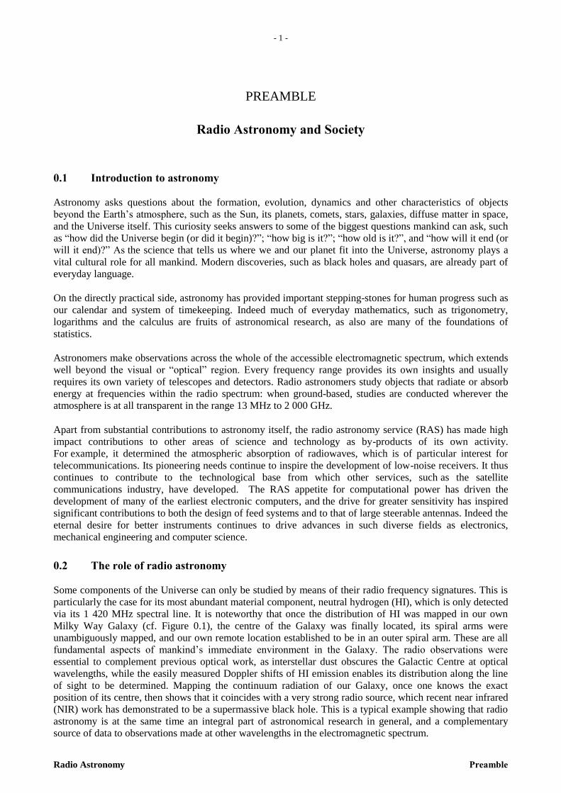
Some components of the Universe can only be studied by means of their radio frequency signatures. This is
particularly the case for its most abundant material component, neutral hydrogen (HI), which is only detected
via its 1 420 MHz spectral line. It is noteworthy that once the distribution of HI was mapped in our own
Milky Way Galaxy (cf. Figure 0.1), the centre of the Galaxy was finally located, its spiral arms were
unambiguously mapped, and our own remote location established to be in an outer spiral arm. These are all
fundamental aspects of mankind’s immediate environment in the Galaxy. The radio observations were
essential to complement previous optical work, as interstellar dust obscures the Galactic Centre at optical
wavelengths, while the easily measured Doppler shifts of HI emission enables its distribution along the line
of sight to be determined. Mapping the continuum radiation of our Galaxy, once one knows the exact
position of its centre, then shows that it coincides with a very strong radio source, which recent near infrared
(NIR) work has demonstrated to be a supermassive black hole. This is a typical example showing that radio
astronomy is at the same time an integral part of astronomical research in general, and a complementary
source of data to observations made at other wavelengths in the electromagnetic spectrum.
- 2 -
Preamble Radio Astronomy
FIGURE 0.1
The central plane of our Galaxy with the Galactic Centre in the middle. The upper frame shows the radio
continuum structure at 408 MHz. The middle frame shows the integrated neutral hydrogen emission at
1 420 MHz. The lower frame shows the central region in optical light and displays the dark dust structures
Radio-Astro_01
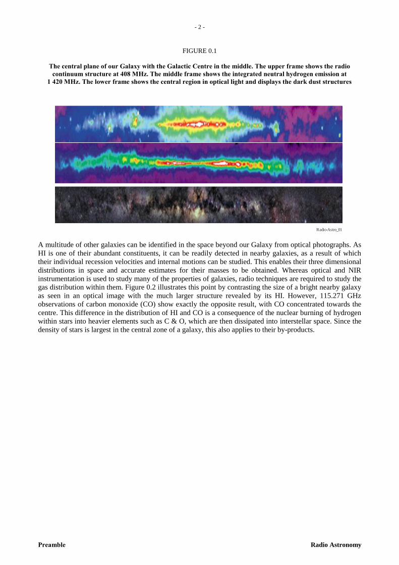
A multitude of other galaxies can be identified in the space beyond our Galaxy from optical photographs. As
HI is one of their abundant constituents, it can be readily detected in nearby galaxies, as a result of which
their individual recession velocities and internal motions can be studied. This enables their three dimensional
distributions in space and accurate estimates for their masses to be obtained. Whereas optical and NIR
instrumentation is used to study many of the properties of galaxies, radio techniques are required to study the
gas distribution within them. Figure 0.2 illustrates this point by contrasting the size of a bright nearby galaxy
as seen in an optical image with the much larger structure revealed by its HI. However, 115.271 GHz
observations of carbon monoxide (CO) show exactly the opposite result, with CO concentrated towards the
centre. This difference in the distribution of HI and CO is a consequence of the nuclear burning of hydrogen
within stars into heavier elements such as C & O, which are then dissipated into interstellar space. Since the
density of stars is largest in the central zone of a galaxy, this also applies to their by-products.
- 3 -
Radio Astronomy Preamble
– 3
–
FIGURE 0.2
The face-on galaxy NGC 6946 is shown in visible light (left) and in neutral hydrogen1 (HI) line emission at
1 420 MHz (right) on the same scale. The neutral hydrogen emission shows large-scale spiral arm structures that
extend far beyond the optical image and reveal the dynamics of the galaxy. At many locations (particularly the
“holes” in the distribution) high-velocity gas outflows are correlated with ongoing star formation.
Radio data from the Westerbork Synthesis Radio Telescope, The Netherlands
Radio-Astro_02
Many radio sources were found as a result of early continuum surveys of the sky at radio frequencies: it then
became a competition to find their optical identifications. Among the most notable surprises was the
discovery of pairs of radio sources mostly equally spaced on opposite sides of some galaxies, indicating
enormous zones of radio emission associated with, but well separated from them as seen in their optical
images. As instrumental techniques improved and studies were made at higher frequencies, it became
apparent that these emission zones were the remnants of highly relativistic jets emanating from the galactic
nuclei. This is also a feature of quasars, which are now recognized to be super-massive black holes accreting
mass at the centres of their host galaxies. Relativistic jets, which commonly require the use of radio
techniques for their study, are a recurrent theme in modern-day astronomy, since the physics behind them is
not fully understood and they occur whenever mass is being actively accreted onto a dense object, whether
this is a super-massive black hole, a stellar sized black hole, a neutron star, or even the degenerate core of a
normal star.
Radio astronomers have provided major contributions to our understanding of the Universe as an entity. This
began with the 1964 discovery of the almost isotropic cosmic microwave background (CMB), for which the
1978 Nobel Prize was awarded, the second to radio astronomers. Continuum observations of the sky at
frequencies between 30 and 300 GHz show that the CMB has a 2.73 K brightness temperature. The CMB is
attributed to thermal radiation from ionised gas which filled the Universe immediately following its origin in
a Big Bang; i.e. from the time that the Universe first became opaque to radio emission. It is the earliest
‘fossil’ signal that is observable. With its discovery the Big Bang paradigm became the accepted
macroscopic description of the history of our Universe and eliminated the Steady State paradigm from
contention. In 1992 an all-sky survey of the CMB using satellite-borne instruments resulted in the detection
of both the Doppler signature of the Earth/Sun/Galaxy movement with respect to the CMB and also the
existence of small, point-to-point variations (a few parts in 10-5
) in its brightness temperature. The 2006
Nobel Prize recognized these landmark measurements. Yet more sensitive measurements of faint structure in
____________________
1 Boomsma, R., Oosterloo, T. A., Fraternali, F., Van Der Hulst, J. M., Sancisi, R., Astronomy and Astrophysics, 490, 555 (2008).
- 4 -
Preamble Radio Astronomy
its intensity have introduced a new era of precision cosmology by greatly refining the cosmological
parameters describing the Universe, and providing independent confirmation that its expansion rate is
accelerating, something that was originally not expected. Future satellite missions expect to exploit the
polarisation properties of the CMB.
Moving from the very large scale to the very small, neutron stars were predicted to exist in 1934, soon after
the discovery of the neutron. Their observational discovery in 1967 in the form of rapidly pulsating radio
sources (pulsars) was recognized with the 1974 Nobel Prize, the first to be awarded to radio astronomers.
One of the major opportunities afforded by pulsars is as laboratories for fundamental physics. A particular
group of pulsars, which rotate very rapidly with millisecond periods, can act as highly accurate clocks. Some
of these are in orbit about a companion, and the combination of an accurate clock in close orbit about a
companion object, whether it is a neutron star, a white dwarf or a more normal star, enables the
determination of highly accurate orbits and pulsar masses, as well as the extensive testing of many
predictions of General Relativity. The General Relativistic description of the evolution of the orbit of the first
pulsar to be discovered in a binary stellar system provided the first demonstration for the predicted existence
of gravitational wave radiation, for which the 1993 Nobel Prize was awarded. In 1992 the first planet
discovered beyond the Solar System was identified from its influence on the timing solution of a pulsar.
The detailed physics applicable within a neutron star changes with its mass, so the equations used to describe
its nuclear matter become more complex as the mass of a pulsar increases. Most pulsars have masses close to
the 1.4 solar mass Chandrasekhar limit. Not surprisingly, there is great interest in discovering objects with
masses of 2 or more solar masses, as their mere existence constrains their possible equations of state, since
these are expected to be influenced by admixtures of exotic forms of matter in their cores. There are no other
means of testing the applicable physics. Likewise, otherwise inaccessible physics can be tested by
observations of a rare set of pulsars, the magnetars. These have ultra-strong magnetic fields, which are well
beyond our capacity to generate in laboratories. On a different research frontier, an extensive worldwide
campaign is being conducted to use timing observations from an all-sky set of millisecond pulsars with the
hope of directly detecting gravitational waves in the nanohertz frequency range.
0.3 Economic and societal value
0.3.1 Introduction
It is difficult to assess the economic value of the use of the radio frequency spectrum for scientific research
and its applications by simply quantifying its costs and benefits in comparison with an alternative use of the
spectrum. The spin-off aspects of radio astronomy on the economy must also be considered. Technical
innovations by radio astronomers have been implemented in many applications that benefit society as a
whole. For example, spin-offs from radio astronomy receiver research (see § 0.3.2.1) are found in specialized
telecommunication equipment as well as in mass-produced consumer applications. It is similarly difficult to
estimate the economic and societal benefits of medical imaging algorithms that have been derived originally
from radio astronomical imaging techniques (see § 0.3.2.4).
0.3.2 Economic and societal value of radio astronomy research
Progress in radio astronomy depends on advances in receiver and digital technology. As a rule, radio
astronomy instrumentation uses the most advanced technology, and astronomers play an active role in
pushing this to its practical limit. The following subsections present examples of radio astronomy research
activities that have been incorporated into applications with other societal value.
0.3.2.1 Telecommunication technology
Receiver systems
Radio astronomy systems include high-gain antennas, low-noise receivers, solid-state oscillators and
frequency multipliers. The development of parametric amplifiers, cryogenically cooled GaAs FET
amplifiers, HEMT amplifiers and SIS mixers were all motivated or influenced by radio astronomy
requirements. These developments have resulted in receivers operating over extremely wide bandwidths and
with temperatures as low as 2 K. The noise temperatures reached at some frequencies are now close to the
quantum limit of what is technically possible. Some of the most sophisticated, deep-space
telecommunication systems use these technologies, their local oscillators being synchronized in time at sub-

- 5 -
Radio Astronomy Preamble
– 5
–
picosecond levels by atomic frequency standards. These standards are used as the backbone of the time-
keeping system for both terrestrial and space navigation systems.
Homology principle
A major obstacle to designing very large, steerable, parabolic antennas with precise reflecting surfaces is
gravitational deformation that changes the shape of an antenna as it moves from one position to the next.
This issue was solved in 1967 by recourse to the homology principle2. An antenna designed with this
principle deforms smoothly under gravitational stress along a sequence of paraboloids with consequential
changes in the focal position. By simply ensuring that the receiver and its feed track this changing focal
position, the effects of gravitational deformation and consequent signal loss are minimised. All large,
reflecting, parabolic antennas now make use of homology. This is of paramount importance when working at
millimeter wavelengths.
Antenna technology
Radio astronomers were the first to use circularly polarised feed horns. Subsequently satellite transmitters
made use of this technical development to transmit both polarisations independently via the same feed horn,
with savings in both package mass and space.
0.3.2.2 Interferometric technology
Radio astronomers developed interferometry both to obtain increased angular resolution and also as an
imaging technique. They then used it to produce digitised single-pixel surveys of the radio sky. Chapter 7
describes the technique, which has since become important in astronomy across the electromagnetic (EM)
spectrum, and also in fibre optics, engineering metrology, optical metrology, oceanography, seismology,
quantum mechanics, nuclear & particle physics, plasma physics and remote sensing.
Radio astronomers were also the first to develop image reconstruction and cleaning techniques for removing
(most) instrumental and environmental effects from images. These methods are used in both terrestrial and
satellite-based surveys of the heavens, as well as by the Earth Exploration Satellite Service (EESS) in
surveying the Earth.
In the latter part of the 20th Century, radio interferometric systems were widely used for facilitating the
automatic landing of aircraft. Indeed, the system was initially developed by a radio astronomy laboratory and
then sold to the world at large. The same technology is now used to locate cell-phone users in order to
provide a rapid response to accident sites by emergency services, as well as to offer targeted marketing and
other location-related services. The Wi-Fi wireless network is a very prominent example of an operational
system.
Wi-Fi applications
Reflections were a major difficulty in developing wireless connections between computer terminals, as a
series of echoes follows the arrival of a transmission at a receiver. This problem was well known to radio
astronomers, who had developed signal processing techniques to overcome comparable issues caused by
reflections in the atmosphere. Radio-based LANs send their data at different frequencies and these signals
are recombined at the receiver in the same manner as in radio astronomy.
Navigation
Over the ages astronomy has made major contributions to navigation both on the ground and in space. The
development of radio sextants for marine navigation has allowed the accurate determination of positions on
overcast and rainy days. A recent application of radio interferometry for emergency position determination
of mobile phones using multilateration is based on the signal strength to nearby antenna masts. This locates
an object by accurately computing the time difference of arrival (TDOA) of a signal emitted from an object
at three or more receivers. It can also be used to locate a receiver by measuring the TDOA of a signal
transmitted from three or more synchronised transmitters.
____________________
2 Von Hörner, S.: “Design of large steerable antennas”, The Astronomical Journal, 72 (1967), 35.
- 6 -
Preamble Radio Astronomy
0.3.2.3 Computing technology
Radio astronomers have developed state-of-the-art digital techniques to correlate and record telescope data.
Modern, high-power (parallel processing) computer-arrays are then used to process extremely large amounts
of data collected by interferometer networks. Simultaneous multi-beam synthesis, real-time mitigation of
RFI and reconstruction of complex radio source structures are examples of modern processing capability.
Indeed radio astronomy data processing for the real time correlation of interferometric data flowing from
antennas on four continents is being used as a test case in the development of large-bandwidth data-network
capability.
Computer Language FORTH
A highly visible spin-off of radio astronomy is the computer language FORTH (or Forth) developed at the
USA NRAO in the early 1970s. The first application of Forth was the control and data processing for one of
the NRAO telescopes. The Forth language is now used in many applications, such as the first hand-held
computers carried by Federal Express delivery agents, and continues to be used today in its evolved forms.
Other applications include satellite tracking software and the simulation software for the Canadian-built, 50-
foot long, six-jointed arm carried on the Space Shuttle. This has been used in satellite deployment and
retrieval operations and to assist astronauts in servicing tasks (e.g. the repair and upgrade of the Hubble
Space Telescope)3.
0.3.2.4 Medical technology
Radio astronomers initiated the mathematical techniques that resulted in the reconstruction of two-
dimensional images from one-dimensional scans, and the reconstruction of three-dimensional ones from two-
dimensional images4. These image reconstruction techniques have been incorporated into modern CT
(Computed Tomography), PET (Positron Emission Tomography) scanning, and magnetic resonance
imaging. Radio observations of distant cosmic sources are basically measures of the temperature of these
sources, and the technique has been adapted to conduct non-invasive measurements of the temperature of
human tissue.
CT is a medical imaging method in which digital computers are used to generate a three-dimensional image
of the inside of an object from a large series of two-dimensional X-ray images taken around a single axis of
rotation.
Malignant tumours appear on microwave images of deep tissue as regions of anomalous temperature and can
be readily detected. Microwave thermography is used with a true-positive detection rate of 96% to detect
breast cancer.
Skin cancer
One of the major challenges for astronomers studying stars and galaxies is to extract meaningful information
from a jumble of signals. Since radio astronomers were the first astronomers to manipulate digital data, they
developed the algorithms used for picking out weak signals from a background of random “noise”. These
algorithms have helped other astronomers to pinpoint thousands of faint X-ray sources and analyse their
structures in a quantitative way.
These techniques are applicable to many other situations where vital data is buried in background noise.
In one collaboration with medical doctors, and with the support of the German Space Agency, radio
scientists developed a system for the early recognition of skin cancer. Small differences in colour can lead to
the detection and measurement of the irregular cell growth associated with malignant melanoma, which is a
particularly virulent form of skin cancer.
____________________
3 For more complete information on the uses of Forth, see, e.g.: http://www.forth.com/index.html.
4 Bracewell, R.N. and Riddle, A.C.: “Inversion of fan beam scans in radio astronomy”, Astrophys. Journal, 150, 427.
- 7 -
Radio Astronomy Preamble
– 7
–
Digital radiography
Digital imaging technology was also adapted to assist in measurements of X-ray emissions from galaxy
clusters, which are important to astrophysicists in developing theories related to cosmology and the early
evolution of the Universe.
The technique was then used in the design of a digital radiography system to improve the efficiency,
flexibility and cost-effectiveness in hospital radiographic examinations. This reduces hospital and emergency
room operating costs by eliminating the expense of film in X-rays and other image acquisition procedures.
Using this technology, radiographic examinations are conducted in the standard manner except that body
images are now stored in the computer’s memory rather than on film. The doctor (and/or patient) can then
view the images immediately, and they can be readily transmitted to distant specialists with full fidelity via
the internet.
0.3.2.5 Time and frequency standards
Out of necessity, the very long baseline interferometry (VLBI) community developed extremely stable and
precise time standards and time transfer methods with uncertainty levels of a few parts in 10-16
s. These
systems were later developed commercially and are now used for satellite navigation, space communication
and defence purposes. The worldwide Radionavigation Satellite Service (RNSS) systems (GPS, Glonass,
Galileo) have their time and coordinate systems tied to the Earth and to the cosmos by the maintenance
activities of the International VLBI Service for Geodesy and Astrometry (IVS).
Accurate man-made clocks ushered in the modern era of safe navigation. The quest for ever more accurate
clocks and the determination of time from an ensemble of atomic clocks are continued by the International
Time Bureau. However, the best independent check on the long-term stability of the international atomic
time standards comes from the timing observations of millisecond pulsars by radio astronomers. These are
conducted on an ensemble of the most stable pulsars, both to minimize any effects of secular changes in the
electron content of the interstellar medium along their lines of sight and also to minimize any erratic
behavior of individual pulsars. It is also independently checked by fitting timing observations of millisecond
pulsars in binary stellar systems to the orbital parameters of the system.
0.3.2.6 Earth observation
Radio astronomy interferometric methods have been adopted to develop passive remote-sensing techniques
for the measurement of the temperature of the Earth’s atmosphere, and also for the determination of other
surface properties, such as the distribution of water vapour, cloud water content, precipitation and the level
of other impurities such as carbon monoxide.
The detection of forest fires from their thermal microwave radiation is based on the same technological
principle.
0.3.2.7 Geodesy
Although the VLBI technique was developed as a tool to gather data on the detailed structure and positions
of astronomical sources, it also has applications for many other purposes. Thus, the extremely accurately
measured VLBI positions of distant quasars and radio sources provide mankind’s most accurate spatial
reference frame. Using celestial sources as reference points allows terrestrial VLBI to measure the inherent
motions of telescopes on the Earth, such as those arising from continental drift or the slippages of tectonic
plates at fault lines. Such measurements help in estimating the likelihood of Earthquakes. The International
VLBI Service for Geodesy and Astrometry (IVS) was established to provide services in support of geodetic,
geophysical and astrometric research and operational activities5. Terrestrial VLBI techniques and accurate
Doppler tracking are also used for high-precision space-navigation missions within our Solar System.
Thus, the position of ESA’s Huygens probe was accurately tracked as it entered the atmosphere of Titan, the
largest moon of Saturn.
____________________
5 See: http://ivscc.gsfc.nasa.gov/html.
- 8 -
Preamble Radio Astronomy
0.3.2.8 Mining technology
The imaging techniques described in § 0.3.2.4 can also be directly applied to the sub-surface exploration for
oil and mineral deposits. Data from an array of seismometers making measurements following a chain of
small surface explosions are processed in a similar manner.
0.3.2.9 Radar astronomy
Radar astronomy differs from radio astronomy in that it involves both the transmission and reception of
radio waves. A consequence of this is that its two-way spreading loss limits it to the study of objects in the
solar neighbourhood. However, it is the only method that can be used to detect small-scale space-debris. A
typical application of radar astronomy is the detection and tracking of Near Earth Objects (NEOs)
(meteorites and asteroids) that come close to the Earth or that may impact the Earth, and it offers the most
comprehensive means of studying them. In this capacity radar astronomy is a planetary-scale, disaster
prediction and prevention service. Furthermore, radar enables the detection of space debris in orbit around
the Earth, which enables satellite operators to move their space vehicles away from potential collisions. It is
also the only way to study the density of space debris of less than approximately 1 cm size.
Radar astronomy imaging techniques (for the near field) are used for civil and military purposes for imaging
spacecraft in orbit.
0.4 Solar Radio Monitoring
0.4.1 Introduction
Solar radio monitoring is a specialised branch of radio astronomy that plays an active role in space weather
research, facilitates space weather forecasting, and provides timely alerts of solar eruptive events that could
impact human activities. Our susceptibility to the Sun’s behaviour has led to the study of “Space Weather” as
a new discipline, in which conditions in space near the Earth are studied by measuring electromagnetic
radiation and the behaviour of solar plasma. On long and intermediate timescales, the impact of solar
variability on the climate ranks in importance at the same level as volcanism and human activity. On shorter
timescales, the role of space weather is also important because of the disruptions that solar events,
particularly coronal mass ejections (CMEs), may cause to our technical infrastructure in space, in the air and
on the ground. CMEs occur once a day or more frequently around solar maximum.
When data from ground-based, radio spectrographs are combined with complementary data from satellites,
estimates of the mass, energy, and speed and direction of propagation of coronal mass ejections can be
obtained long before they reach the Earth. From these measurements the severity of a disturbance and its
probable time of arrival at the Earth can be inferred, thus providing the possibility of mitigating adverse
effects on a wide variety of human technologies, such as telecommunications, satellite-based navigation
systems, space activities (satellites, manned missions), aviation and electrical power grids. Solar activity also
causes a gradual degradation of power transformers, corrosion of long-distance pipelines, and generates
many other adverse effects. The impact of a giant solar flare, which is another less frequent and randomly-
occurring, natural hazard, could also be severe. Such an event, if unmitigated, could cause major worldwide
disruption to our technologically dependent society. An illustrative event occurred in March, 1989, when a
very large flare produced an impact that cost more than 109 US Dollars. Nowadays, unless appropriate
actions were taken prior to its arrival at the Earth, a giant solar flare could cause damage that may be very
much more costly. Indeed some estimates put the likely cost of such an event at 2 to 3x10¹²
US Dollars, in
addition to a 2 to 3 year recovery time, as many replacement items that would be required (e.g. repair of the
power grid) are too expensive to keep as spares. This uncontrollable risk highlights the crucial role of early-
warning systems that rely on continuous solar monitoring facilities, amongst which are ground-based solar
radio telescopes.
There are many ways of monitoring solar activity, one of which is to simply count sunspots. Radio
measurements have the advantage of being made automatically from the ground, of requiring little or no
human intervention, and of being inexpensive. Moreover it is possible to maintain data calibration, quality
and consistency over long periods of time.
- 9 -
Radio Astronomy Preamble
– 9
–
0.4.2 Overview of solar radio monitoring
Radio measurements of the Sun are direct indicators of the level and nature of solar activity. They can also
be used as proxies for other parameters that are difficult or impossible to measure with the required accuracy
and long-term continuity. Solar flux monitors are specially-designed, radio telescopes with antennas that are
small enough to “see” the whole of the solar disc with equal sensitivity, and with receivers having very high,
linear dynamic ranges to measure accurately the solar flux.
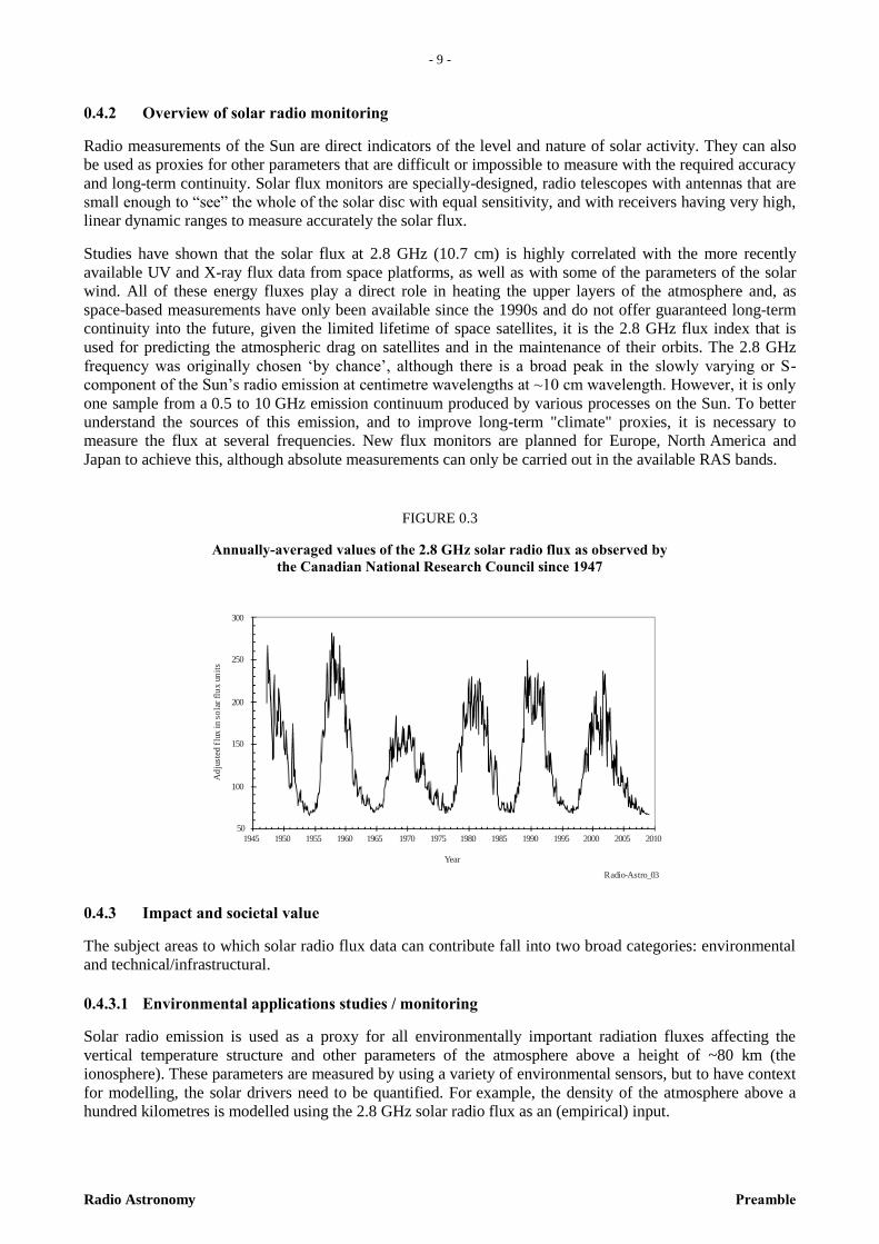
Studies have shown that the solar flux at 2.8 GHz (10.7 cm) is highly correlated with the more recently
available UV and X-ray flux data from space platforms, as well as with some of the parameters of the solar
wind. All of these energy fluxes play a direct role in heating the upper layers of the atmosphere and, as
space-based measurements have only been available since the 1990s and do not offer guaranteed long-term
continuity into the future, given the limited lifetime of space satellites, it is the 2.8 GHz flux index that is
used for predicting the atmospheric drag on satellites and in the maintenance of their orbits. The 2.8 GHz
frequency was originally chosen ‘by chance’, although there is a broad peak in the slowly varying or S-
component of the Sun’s radio emission at centimetre wavelengths at ~10 cm wavelength. However, it is only
one sample from a 0.5 to 10 GHz emission continuum produced by various processes on the Sun. To better
understand the sources of this emission, and to improve long-term "climate" proxies, it is necessary to
measure the flux at several frequencies. New flux monitors are planned for Europe, North America and
Japan to achieve this, although absolute measurements can only be carried out in the available RAS bands.
FIGURE 0.3
Annually-averaged values of the 2.8 GHz solar radio flux as observed by
the Canadian National Research Council since 1947
Radio-Astro_03
1950 1955 1960 1965 1970 1975 1980 1985 1990 1995 2000 2005 2010
100
50
150
200
250
300
Year
Ad
just
ed f
lux
in s
ola
r fl
ux
unit
s
1945
0.4.3 Impact and societal value
The subject areas to which solar radio flux data can contribute fall into two broad categories: environmental
and technical/infrastructural.
0.4.3.1 Environmental applications studies / monitoring
Solar radio emission is used as a proxy for all environmentally important radiation fluxes affecting the
vertical temperature structure and other parameters of the atmosphere above a height of ~80 km (the
ionosphere). These parameters are measured by using a variety of environmental sensors, but to have context
for modelling, the solar drivers need to be quantified. For example, the density of the atmosphere above a
hundred kilometres is modelled using the 2.8 GHz solar radio flux as an (empirical) input.
- 10 -
Preamble Radio Astronomy
0.4.3.2 Technical/Infrastructural uses
Occasionally solar emissions, particularly in the VHF spectrum, are strong enough to degrade radio systems
(e.g. communications) by increasing their noise levels.
Solar-driven effects on satellites
Satellites operate in an environment populated by high-energy particles emanating from the Sun. These can
temporarily degrade or permanently damage electronics, as can an accumulation of charge on a spacecraft,
which may also create phantom commands that disrupt its operation. Satellites in low Earth orbit are also
subject to increases in atmospheric drag that can change their positions and enhance the rates of their orbital
decay. The general level of solar activity indicated by indices, such as the 2.8 GHz solar radio flux, are used
to predict the degree of heating and expansion in the upper atmosphere and the consequences for satellite
orbits.
Ionospheric effects
Since the Sun generates the ionosphere, changes in solar activity result in concomitant changes in the
ionosphere that can result in an enhanced communication capacity or a total blackout lasting for many hours
if solar X-rays significantly increase the degree of ionisation in the D-Region. As the ionosphere is a very
important medium for communications, forecasting of ionospheric conditions is also very important: the ITU
uses radio data both as an ionospheric diagnostic for current conditions and as an aid for predicting their
likely short-term evolution.
Commercial aircraft use HF on their long-distance routes over the poles, since there is no VHF infrastructure
at high latitudes (>82º), and the geosynchronous satellite belt is close to the horizon. As ionospheric
disturbances are particularly common and troublesome at high latitudes, radio measurements of solar activity
are needed to forecast polar ionospheric conditions, in order to provide sufficient notice for airlines to adjust
flight plans as necessary.
Geomagnetic effects on ground systems
Both rapid and slow fluctuations in the Earth’s magnetic field are generated by the changing velocity and
density of the solar wind, and especially by the impact of plasmoid ejected during solar flares and CMEs.
These fluctuations induce electrical currents in long metal structures such as power lines, pipelines, phone
cables and railway tracks. The currents induced in power lines offset the operating points of transformers,
which, if heavily loaded, can lead to saturation of their core and overheating of their windings. However,
major magnetic storms, such as the one of 13 March 1989, produce much larger currents that can lead to
an immediate transformer failure, as indeed it in Quebec, Canada. This brought about the collapse of the
power distribution network for more than nine hours. The economic impact of this infrastructure failure from
the loss of industrial production was of the order of 109 US dollars.

- 11 -
Radio Astronomy Preamble
– 1
1 –
FIGURE 0.4
Burned out transformer from an electrical power distribution network
due to solar activity on 13 March, 1989
Radio-Astro_04
Induced currents in railway tracks can interfere with signalling systems and train position sensing. They also
generate small potential differences across inhomogeneities in a pipeline’s metal and across its welds, which
increases the rate of cathodic corrosion.
Pipelines may span thousands of kilometres, often in a hostile terrain and climate, where inspection and
maintenance may be expensive. However, a failure may be even more expensive with severe environmental
consequences. Thus, inspection and maintenance models based upon geomagnetic activity are required.
0.5 Trends in radio astronomy
Current trends in radio astronomy are towards even higher sensitivities at all frequencies. Since current
receivers are approaching the quantum limit at many frequencies, there is a drive towards larger collecting
areas and the use of broader operational bandwidths. Existing telescopes are being upgraded to accommodate
broadband receivers (from 1 to 8 GHz depending on frequency) for both continuum and spectral line
observations. Some international efforts are underway to construct new-generation radio telescopes with
significantly larger collecting surfaces.
Examples are:
1) the square kilometer array (SKA) project, which seeks to build a giant radio interferometer network
with a total collecting area of one square kilometer and baselines up to 3000 km operating over a
frequency range from 100 MHz to 25 GHz;
2) the low frequency array (LOFAR) in The Netherlands and neighbouring countries is a radio
interferometer network with a total collecting surface of 100,000 m2 and baselines up to 1000 km
operating over a frequency range from 30 to 250 MHz;
3) the Atacama large millimeter/submillimeter Array (ALMA) with 64 antennas on a 5 km high
plateau in the Andes operating over a frequency range from 30 to 850 GHz.
- 12 -
Preamble Radio Astronomy
0.6 Conclusions
Radio astronomy has led to the discovery of totally new and unpredicted radio phenomena, such as the
Cosmic Microwave Background, interstellar ionised gas and plasmas, as well as pulsars, quasars and black
holes. It has also provided many validation checks of the fundamental theories of physics, such as General
Relativity, and has provided a laboratory for otherwise inaccessible fundamental physics.
The spectrum used by the radio astronomy service has considerable societal and economic value, although it
is difficult to quantify the benefits, as these are enjoyed by society as a whole, are often resident within
applications developed by other technologies, are often realized over very long periods of time, and may be
difficult to foresee. The RAS has developed technologies with widespread applications in such diverse fields
as medical diagnostics, telecommunications, time and frequency standards, Earth observations, computing,
navigation, geophysics and mining.
Many RAS activities are organized at a global level and spectrum related issues must therefore be considered
globally, since unilateral decisions can have a worldwide impact on related frequency use and possible
measurements.
Instabilities in the magnetic field of the Sun can generate energetic solar flares and trigger coronal mass
ejection events. These are capable of directly degrading or damaging many electronic-based technologies
and Earth-based infrastructure, with great consequential cost. The monitoring of solar radio emission from
the ground has provided a reliable, consistent and inexpensive means of monitoring solar activity for over 60
years. It is a mature, well-understood technology that provides timely warnings of transient events.
- 13 -
Radio Astronomy Chapter 1
– 1
3 –
CHAPTER 1
Introduction
1.1 The Radiocommunication Sector and World Radiocommunication Conferences
This Handbook is concerned principally with aspects of radio astronomy that are relevant to frequency
coordination, that is, the usage of the radio spectrum in a regulated manner to avoid interference by mutual
agreement between the radio services. On an international scale, spectrum usage is regulated through the
International Telecommunication Union (ITU), which is a specialized agency of the United Nations
Organization.
The Radiocommunication Sector (ITU-R), which is a part of ITU, was created on 1 March 1993; it replaced
the International Consultative Committee on Radio (CCIR) and its Secretariat, which performed similar
functions up to then. ITU-R includes World and Regional Radiocommunication Conferences,
Radiocommunication Assemblies, the Radio Regulations Board, Radiocommunication Study Groups, the
Radiocommunication Advisory Group and the Radiocommunication Bureau that is headed by an elected
Director.
The ITU Radio Regulations, which are the basis of the planned usage of the spectrum, are the result of World
Radio Conferences (WRCs), formerly known as World Administrative Radio Conferences (WARCs), which
are held at intervals of a few years. At such conferences, the aim is to introduce new requirements for
spectrum usage in a form which is, as far as possible, mutually acceptable to the representatives of
participating countries. The results of each WRC take the form of a treaty to which the participating
administrations are signatories. WRCs also develop an Agenda for the next WRC, and Resolutions, that
usually include calls for studies related to the future Agenda items to be carried out by the Study Groups. As
in most areas of international law, the enforcement of the regulations is difficult, and depends largely upon
the goodwill of the participants. WRCs are preceded by Conference Preparatory Meetings (CPMs) that
elaborate reports on technical, operational and regulatory matters to be considered by the Conference.
Radiocommunication Study Groups (SGs) are set up by a Radiocommunication Assembly. They study
questions and prepare draft recommendations on the technical, operational and regulatory/procedural aspects
of radiocommunications. The ITU-R SGs address such issues as preferred frequency bands for the various
services, threshold levels of unacceptable interference, sharing between services, desired limits on emissions,
etc. They also provide input to the draft CPM Report on Agenda items of their competence. The SGs are
further organised into Working Parties (WPs) and Task Groups (TGs) which deal with specific aspects of the
work. At present (2013) the ITU-R SG structure is as follows:
Study Group 1 Spectrum management
Study Group 3 Radiowave propagation
Study Group 4 Satellite services
Study Group 5 Terrestrial services
Study Group 6 Broadcasting service
Study Group 7 Science services
In addition to these, the Coordinating Committee for Vocabulary (CCV) and the Special Committee for
Regulatory and Procedural Matters (SCRPM) have responsibilities over matters common to all groups.
More information about the ITU-R, details about the SGs and WPs, and about their work and documentation
can be found on the ITU-R website:
http://www.itu.int/ITU-R/index.asp?category=information&rlink=rhome&lang=en.
- 14 -
Chapter 1 Radio Astronomy
Working Party 7D, that deals with radio astronomy, is one of the four Working Parties within ITU-R SG 7,
Science services, which also includes WPs dealing with space operations, space research, passive and active
remote sensing, meteorology, and time signals and frequency standards. The search for extraterrestrial
intelligence (SETI), and radar astronomy as practiced from the surface of the Earth, as well as radio
astronomy conducted from space under the space research service are usually included with radio astronomy
in the work of WP 7D.
International meetings of the Study Groups and Working Parties occur at regular intervals, usually twice a
year, and are attended by delegations from many countries. Task Groups are set up for a limited period of
time to carry out specific tasks, and meet at intervals according to their needs. The working methods of the
Study Groups and their Working Parties are described in detail in ITU-R Resolution 1. In general, the SGs
and WPs respond to appropriate Questions assigned to them. Responses to these Questions are provided
generally in the form of ITU-R Recommendations or Reports.
The ITU-R Recommendations provide a body of technical, operational and regulatory/procedural
information that has been agreed upon by the participating administrations. This information is also used to
provide inputs developed in response to specific WRCs Agenda items, and many of the results of the work of
the Study Groups are thereby incorporated into the Radio Regulations. Aside from this, the ITU-R
Recommendations and Reports are, in themselves, generally regarded as authoritative guidelines for
spectrum users. This is particularly true of the ITU-R Recommendations which, while not of a mandatory
character, are widely followed, and are revised and published regularly. Most of the important material on
radio astronomy in Study Group 7 Recommendations and Reports forms the basis of this Handbook.
1.2 The Radio Regulations and frequency allocations
International frequency allocations are carried out at WRCs, to some 40 radio services defined in the Radio
Regulations. WRCs are attended by representatives of more than 190 ITU Member administrations from all
over the world, by many telecommunication and information technology companies, and by recognized
scientific and international organizations. Only Member administrations may present proposals and have
voting rights, other organizations may, however try to influence the outcome of the various agenda items
through other means. A more complete description of how WRCs work and radio astronomers participate\ion
in them was given, e.g. by Gergely [2002].
For spectrum allocation purposes the world is divided into three regions: Region 1 includes Europe, Africa
and northern Asia; Region 2 includes North America and South America; Region 3 includes southern Asia
and Australasia. For any particular frequency band, the allocations may be different in different regions.
Bands are often shared between two or more services. Generally speaking, the allocations may be primary or
secondary. A service with a primary allocation may cause interference to a secondary service, but a
secondary service is not permitted to cause interference to a service with a primary allocation in the same
band. The frequency allocations are contained in Article 5 of the Radio Regulations. Most are shown in
a table of allocations; however, additional allocations are contained in numbered footnotes to the table.
Within individual countries, spectrum allocation matters are handled by government agencies that vary
greatly from one administration to another. In many countries, the administration of the radio spectrum is
part of the work of a larger agency which may also include areas such as postal and telephone services,
transportation, commerce, etc. Such agencies play major roles in the preparation of national positions that are
advocated at WRCs. Administrations participating in the WRC treaties retain sovereign rights over the
spectrum within their national boundaries, and can deviate from the international regulations to the extent
that this does not cause harmful interference within the territories of other administrations. In the setting up
of the Radio Regulations, many administrations have claimed exceptions in certain bands in order to cover
particular national requirements.
1.3 Radio astronomy as a radiocommunication service
Radio astronomy was first officially recognized as a radiocommunication service at the WARC-59. At that
time, under the auspices of the International Council of Scientific Unions (ICSU), three scientific unions set
up a commission, the Inter-Union Commission for the Allocation of Frequencies for Radio Astronomy and
Space Science (IUCAF) to represent scientific usage of the radio spectrum. The three founding unions are
the International Astronomical Union (IAU), the International Union of Radio Science (URSI), and the
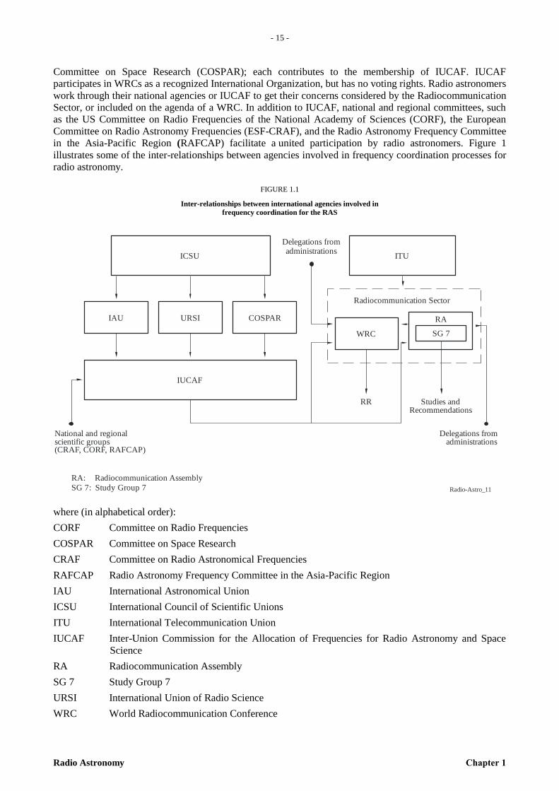
- 15 -
Radio Astronomy Chapter 1
– 1
5 –
Committee on Space Research (COSPAR); each contributes to the membership of IUCAF. IUCAF
participates in WRCs as a recognized International Organization, but has no voting rights. Radio astronomers
work through their national agencies or IUCAF to get their concerns considered by the Radiocommunication
Sector, or included on the agenda of a WRC. In addition to IUCAF, national and regional committees, such
as the US Committee on Radio Frequencies of the National Academy of Sciences (CORF), the European
Committee on Radio Astronomy Frequencies (ESF-CRAF), and the Radio Astronomy Frequency Committee
in the Asia-Pacific Region (RAFCAP) facilitate a united participation by radio astronomers. Figure 1
illustrates some of the inter-relationships between agencies involved in frequency coordination processes for
radio astronomy.
FIGURE 1.1
Inter-relationships between international agencies involved in
frequency coordination for the RAS
Radio-Astro_11
ICSU
Delegations fromadministrations
IAU URSI COSPAR
IUCAF
WRC SG 7
RA
Radiocommunication Sector
RR Studies andRecommendations
Delegations fromadministrations
National and regionalscientific groups(CRAF, CORF, RAFCAP)
RA: Radiocommunication Assembly
SG 7: Study Group 7
ITU
where (in alphabetical order):
CORF Committee on Radio Frequencies
COSPAR Committee on Space Research
CRAF Committee on Radio Astronomical Frequencies
RAFCAP Radio Astronomy Frequency Committee in the Asia-Pacific Region
IAU International Astronomical Union
ICSU International Council of Scientific Unions
ITU International Telecommunication Union
IUCAF Inter-Union Commission for the Allocation of Frequencies for Radio Astronomy and Space
Science
RA Radiocommunication Assembly
SG 7 Study Group 7
URSI International Union of Radio Science
WRC World Radiocommunication Conference
- 16 -
Chapter 1 Radio Astronomy
In Article 1, Section 1 of the Radio Regulations, radio astronomy is defined as astronomy based on the
reception of radio waves of cosmic origin. In the table of frequency allocations, frequency bands which offer
the greatest protection to radio astronomy are those for which the radio astronomy service has a primary
allocation shared only with other passive (non-transmitting) services. Next in degree of protection are the
bands for which radio astronomy has a primary allocation but shares this status with one or more active
(transmitting) services. Less protection is afforded where bands are allocated to radio astronomy on a
secondary basis.
For many frequency bands, the protection is provided by footnotes in the Radio Regulations rather than by
direct entry in the table of allocations. The footnotes are of several types. For a band allocated exclusively to
passive services, RR footnote No. 5.340 points out that all emissions are prohibited in the band.
Other footnotes are used when radio astronomy has an allocation in only part of the band appearing in the
table. A different form of footnote is used for bands or parts of bands which are not allocated to radio
astronomy, but which are nevertheless used for astrophysically important observations. It urges
administrations to take all practicable steps to protect radio astronomy when making frequency assignments
to other services. Although such footnotes provide no legal protection, they have often proven valuable to
radio astronomy when coordination with other services is required. The frequency bands allocated to the
radio astronomy service are listed in Appendix 1 to this Handbook.
1.4 Frequency allocation problems for radio astronomy
Several features of radio astronomy are different from those of the majority of services that use the radio
spectrum. Radio astronomy is a passive service, concerned only with the reception of data. A few other
services, such as Earth exploration by satellite, also use passive sensing.
Radio astronomy signals are very weak, with power flux densities many orders of magnitude (tens of dBs)
below those utilised by most other services. The highly sensitive receiving systems that are required in radio
astronomy are very vulnerable to interference. This vulnerability is exacerbated by the nature of the cosmic
signals. Most signals have the form of random noise, with no characteristic modulation that would allow
them to be distinguished from other signals. The sharing of frequency bands with active services is difficult,
and is usually possible to share only when there is no direct line-of-sight between a radio astronomy
antenna and a transmitter in the same band. A further problem is posed by unwanted emissions produced in a
radio astronomy band by active services operating in other bands. This is becoming more problematic as the
use of broadband digital-modulation, ultra-wide band and spread-spectrum techniques continues to increase.
The extensive use of unlicensed wireless devices, e.g. smartphones, tablets or laptop computers that can be
easily carried to or deployed in the vicinity of a radio telescope further exacerbates this problem. Because of
this potential threat to radio astronomy, mere preservation of allocations is not sufficient to guarantee
interference-free radio astronomical observations.
Radio astronomers cannot always choose their frequencies arbitrarily. Many of the cosmic signals that they
study take the form of spectral lines covering a limited frequency range. These lines are generated at
characteristic frequencies associated with transitions between quantised energy states of atoms or molecules.
Thus, allocations for observation of these lines must be made at specific frequencies. Allocations for many of
the more important lines were obtained in the past, when the radio spectrum was less heavily used by other
services. Important new lines continue to be detected, and many of them are not within allocated bands. For
spectral lines in distant galaxies, an observed frequency that normally falls within a radio astronomy band
may be Doppler shifted outside the band because of the large motions of the galaxies relative to the Earth.
Therefore, practically all parts of the radio spectrum are of potential scientific interest. However, because of
allocations to active services, observations at many frequencies are severely restricted, or not even possible.
In some cases, it may be possible to minimize interference by choosing appropriate locations for telescopes,
or times for observation. Additional radio astronomy allocations would be desirable, but will be difficult to
obtain for various reasons. Each WRC develops a draft Agenda for the next conference and a provisional
Agenda for the one after. Therefore, even in the best case, a large lead time and sustained effort is required
for any Agenda item to reach a conference. Proposals for future agenda items are submitted by
administrations that, as a rule, tend to select those proposals that they believe are in their most pressing
national interests, so other services may be given higher priority. Even when a radio astronomy related
Agenda item is supported by administrations with an interest in the science, there are relatively few such
administrations within the ITU, where most decisions are reached by consensus.
- 17 -
Radio Astronomy Chapter 1
– 1
7 –
Because radio astronomers have great difficulty in sharing frequencies with active services, and cannot
choose their frequencies arbitrarily, radio astronomy is not easily accommodated within the system of
allocations and regulations. Nevertheless, the passive services are well regarded, not least because the series
of bands allocated to radio astronomy enabled a stream of important scientific discoveries to be made, and
continue to be vital to the existence of the service.
REFERENCES
Gergely, T. [2002] World Radiocommunication Conferences in “Spectrum Management for Radio
Astronomy; proceedings of the IUCAF summer school held at Green Bank, W. VA, June 9-14, 2002, Eds.
B.M. Lewis and D.T. Emerson, Charlottesville, VA.
- 18 -
Chapter 2 Radio Astronomy
CHAPTER 2
Characteristics of the Radio Astronomy Service
2.1 The RAS
Radio astronomy and the RAS are defined in RR Article 1, RR Nos. 13 and 58 as being astronomy based
upon the reception of cosmic radio waves. The aggregate of these cosmic emissions constitutes the cosmic
background noise of communications engineering. Being a passive service, radio astronomy does not involve
the transmission of radio waves in its allocated bands, so the use of these bands does not cause interference
to any other service. On the other hand, the extreme weakness of cosmic radio emissions when compared to
the strength of man-made transmissions makes radio astronomical observations very susceptible to
interference from other radio services. At present, radio astronomy utilises the electromagnetic spectrum at
frequencies from below 1 MHz to about 1 000 GHz, a range set primarily by the limitations of available
technology. In principle, the entire radio spectrum is of scientific interest to the RAS.
Radio astronomy began in 1932, when Karl G. Jansky discovered the existence of radio waves of
extraterrestrial origin [Jansky, 1935]: it is now a well-established and important branch of observational
astronomy. Within the Solar System, it has increased our knowledge of the Sun (e.g. the physical processes
responsible for the radio emissions of plasmas), of the planets, and of interplanetary space. On a larger scale,
multi-frequency studies of cosmic sources of radio emission provide information about interstellar gas clouds
and the star formation within them, about interstellar magnetic fields, about the structure and evolution of
galaxies, and about the cosmological parameters of the Universe as a whole. On the other hand spectral-line
emissions from atoms and molecules at naturally occurring frequencies inform us about the composition,
motions, and physical characteristics of interstellar gas clouds. Much of the knowledge derived from radio
astronomy is unique and not available except from radio wavelengths. Thus for example, atomic neutral
hydrogen (HI), the primeval element of the Universe, is only detectable through its radio line at 1 420 MHz,
and its distribution and motion can only be studied by measuring the intensity and Doppler shifts of this
radiation.
In the study of cosmic radio sources, radio astronomers measure all of the properties of electromagnetic
radiation. These are its intensity, frequency, polarisation, direction (position in the sky), and the temporal
variations of these parameters. Cosmic radio emission usually has a low power flux-density at the Earth.
Most emissions show the characteristics of random noise. Exceptions to this are a) the pulsed emissions at
extremely regular rates from pulsars; b) interplanetary and ionospheric scintillations of small diameter radio
sources; c) irregular bursts from some stars (including the Sun); d) variations on the scale of months for
some radio sources, including effects related to gamma-ray bursts; and e) variations associated with the
planet Jupiter. The best times for observation of radio sources are generally dictated by natural phenomena,
such as the position of the source in the sky and the rotation of the Earth. In contrast to the situation in active
(transmitting) services, radio astronomers cannot change the character of the received signal; nor its emitted
power, nor can the signal be coded in order to increase its detectability. For a review of radio astronomy,
including instrumentation, major results and astrophysical interpretation, see Burke and Graham-Smith,
2002.
2.2 Origin and nature of cosmic radio emissions
Several distinct mechanisms generate cosmic radio emission. Thermal radiation is emitted by anything with a
temperature above absolute zero. It is emitted in particular by hot plasma as well as by neutral gas
(interstellar gas clouds, hot envelopes of stars etc.), and by solid bodies. Moreover, the universal microwave
background is believed to be the residual thermal radiation from hot gas at a very early stage in the
development of the Universe. Non-thermal emission, on the other hand, is mainly synchrotron radiation,
which arises from relativistic electrons spiraling in a magnetic field. This includes gyro-synchrotron and
electron-cyclotron maser emission, as well as plasma-wave emission. Finally, spectral-line radiation arises
from transitions between the energy states of individual atoms and molecules.
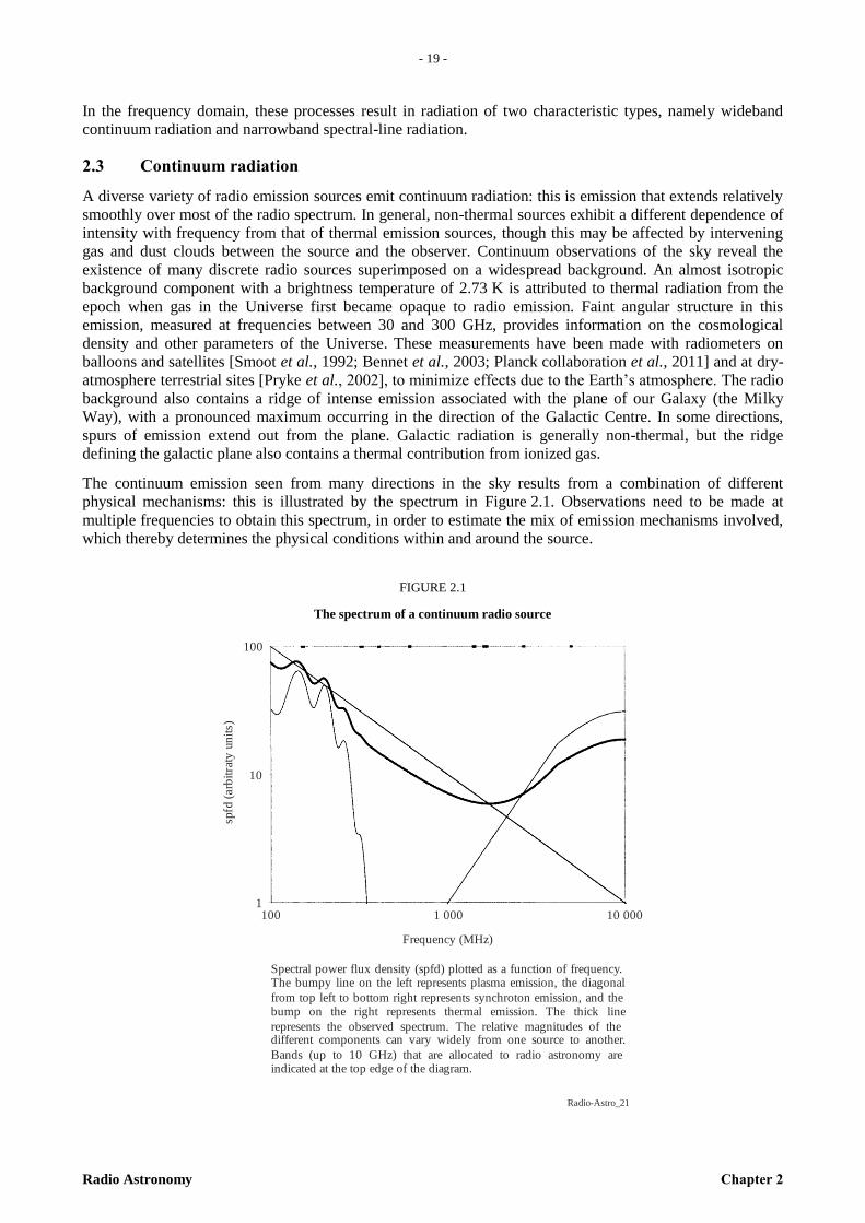
- 19 -
Radio Astronomy Chapter 2
– 1
9 –
In the frequency domain, these processes result in radiation of two characteristic types, namely wideband
continuum radiation and narrowband spectral-line radiation.
2.3 Continuum radiation
A diverse variety of radio emission sources emit continuum radiation: this is emission that extends relatively
smoothly over most of the radio spectrum. In general, non-thermal sources exhibit a different dependence of
intensity with frequency from that of thermal emission sources, though this may be affected by intervening
gas and dust clouds between the source and the observer. Continuum observations of the sky reveal the
existence of many discrete radio sources superimposed on a widespread background. An almost isotropic
background component with a brightness temperature of 2.73 K is attributed to thermal radiation from the
epoch when gas in the Universe first became opaque to radio emission. Faint angular structure in this
emission, measured at frequencies between 30 and 300 GHz, provides information on the cosmological
density and other parameters of the Universe. These measurements have been made with radiometers on
balloons and satellites [Smoot et al., 1992; Bennet et al., 2003; Planck collaboration et al., 2011] and at dry-
atmosphere terrestrial sites [Pryke et al., 2002], to minimize effects due to the Earth’s atmosphere. The radio
background also contains a ridge of intense emission associated with the plane of our Galaxy (the Milky
Way), with a pronounced maximum occurring in the direction of the Galactic Centre. In some directions,
spurs of emission extend out from the plane. Galactic radiation is generally non-thermal, but the ridge
defining the galactic plane also contains a thermal contribution from ionized gas.
The continuum emission seen from many directions in the sky results from a combination of different
physical mechanisms: this is illustrated by the spectrum in Figure 2.1. Observations need to be made at
multiple frequencies to obtain this spectrum, in order to estimate the mix of emission mechanisms involved,
which thereby determines the physical conditions within and around the source.
FIGURE 2.1
The spectrum of a continuum radio source
Radio-Astro_21
Frequency (MHz)
spfd
(arb
itra
ty u
nit
s)
Spectral power flux density (spfd) plotted as a function of frequency. The bumpy line on the left represents plasma emission, the diagonal
from top left to bottom right represents synchroton emission, and the bump on the right represents thermal emission. The thick line
represents the observed spectrum. The relative magnitudes of the different components can vary widely from one source to another.
Bands (up to 10 GHz) that are allocated to radio astronomy are indicated at the top edge of the diagram.
100 1 000 10 0001
10
100
- 20 -
Chapter 2 Radio Astronomy
Most discrete sources located off the galactic plane are extragalactic. These are mainly non-thermal sources
that are identified optically with distant galaxies and quasi-stellar objects (quasars) that are distributed more
or less randomly over the sky. Radio observations of such sources have resulted in a model consisting of an
active galactic nucleus (AGN) with a massive central object, which may be a black hole, surrounded by an
accretion disk with inflowing gas and outflowing jets of highly energetic particles that interact with magnetic
fields to produce extended regions of radio emission. On the other hand, most objects within a few degrees
of the galactic plane belong to our Galaxy. These include thermal sources associated with regions of ionized
hydrogen (HII regions), or stars (including the Sun), or planets, as well as non-thermal sources associated
with supernova remnants (the expanding remains of exploded stars). Radio emission from HII regions and
supernova remnants in nearby galaxies is also observed.
The non-thermal radiation observed from extragalactic sources and sources in the galactic plane (including
both the background and supernova remnants), is often partially linearly polarised. This radiation is
synchrotron radiation, produced by electrons rotating (and hence accelerating) in magnetic fields that are
linearly polarised with an intrinsic polarisation direction perpendicular to that of the magnetic field. Thus, the
existence of polarisation in cosmic radio emission implies the presence of significant order in the associated
magnetic fields. Studies of the polarised radiation from supernova remnants have provided insight into the
interaction of the remnants with the surrounding interstellar magnetic fields. However, the intrinsic direction
of polarisation usually differs from the observed direction, because it has undergone Faraday rotation by
electrons in magnetic fields between the radiation source and the Earth. Since Faraday rotation varies as the
inverse square of the frequency, it can be measured by using polarisation observations taken over a range of
frequencies. Faraday rotation studies therefore provide a powerful means for studying the electron densities
and magnetic fields present in the interstellar medium.
Several phenomena of astrophysical interest are observable only at frequencies of 30 MHz or lower.
Examples include absorption of continuum emission by foreground ionized-gas in our Galaxy, self-
absorption in radio galaxies and quasars, and low-frequency emission from tenuous plasma present in
clusters of galaxies.
2.3.1 Time variability of continuum radiation
The variability of continuum emission with time is relatively common. It may take different forms: bursts
that persist from sub-nanoseconds to hours, pulsating emission with repetition periods ranging from milli-
seconds to seconds, non-periodic changes taking place over weeks or months, or periodic sinusoidal
variations.
An outstanding source of short-period bursts of radio energy of many types is the Sun, whose bursts yield
important knowledge about the plasma physics processes involved [McLean and Labrum, 1985]. These
bursts are most intense at frequencies below 300 MHz. Moreover, bursts arising from disturbances in the
solar atmosphere may progressively increase in frequency during their lifetimes. Correlated radio and optical
flares have been detected from other stars, while the planet Jupiter is also a source of intense bursts that
occur sporadically at frequencies below 30 MHz [Roberts, 1963].
Jupiter has a special form of variability in addition to the constant thermal emission from its disk and the
above-mentioned bursts, since its magnetosphere has van Allen belts. These generate polarised, non-thermal,
synchrotron emission, which is highly beamed and concentrated towards its equatorial belts. As its magnetic
axis is offset from its rotational axis, both the intensity and the polarisation direction of Jupiter’s non-thermal
emission observed at the Earth vary sinusoidally as the planet rotates.
White dwarf stars with strong magnetic fields often show strong flares in the radio regime on frequencies up
to several GHz enabling the study of the plasma in their atmosphere.
The Earth’s ionosphere and the interplanetary medium of the Solar System may cause the observed radio
emission from sources of small angular size to scintillate at a rate that can be as high as several Hertz. Both
the source size, and details on the inhomogeneity and motions of the interplanetary medium can be derived
from the characteristics of this scintillation. While some pulsars are observed to scintillate, this is caused by
the interstellar, rather than the interplanetary, medium.
- 21 -
Radio Astronomy Chapter 2
– 2
1 –
Some radio sources, in particular quasars, show radio emission variability on a time scale of weeks. The
radio emission of optically identified sources such as supernovae, novae, and X-ray sources changes in step
with variations in optical brightness.
Perhaps the most astrophysically interesting sources of pulsed radiation are pulsars. Their extremely regular
pulsed emission was discovered in 1967 [Hewish et al., 1968]. Pulsars are stars composed almost entirely of
neutrons (i.e. from matter in a very condensed state), and most of those known are located in our Galaxy
with pulse periods ranging from 1 millisecond up to 8 s. While the pulse period is set by the rotation of the
star, the duration of the pulse, which depends upon the angle between the line of sight (LoS) to the observer
and the rotation axis of the star, is typically a few percent of the pulse period. Pulsar emission is usually
observed in the frequency range 30 MHz-3 GHz using pulse-averaging techniques: it often requires
integration times of several hours to define their mean pulse profiles. Some pulsars have pulses that are
intrinsically linearly polarised. In their passage through the interstellar medium to the Earth, all pulses are
dispersed, and their direction of polarisation changed by Faraday rotation (see § 2.3.2). Measurements of the
dispersion together with the Faraday rotation allow the electron density and magnetic field strength along the
LoS to be determined. Similarly, pulse arrival-time measurements extending over several years allow the
positions & motions of pulsars across the sky (proper motions) to be determined. Data on the long-term
stability of pulsars, particularly those with millisecond periods, support their potential use as future standard
clocks for time services (see Chapter 7). A worldwide collaboration of observers is timing a set of
millisecond pulsars in the expectation that this cutting-edge project will eventually enable them to directly
detect gravitational wave radiation.
Pulsars have surface magnetic field intensities that are estimated to be in the range 104 – 10
9 Tesla, and, in
the extreme cases of Magnetars, of even reaching 1010
T. The strong magnetic field combined with the fast
rotation induces strong electric fields and creates a dense relativistic plasma around the neutron star carrying
a strong current. Strong coherent radio emission is seen as a by-product of energy dissipation in the
magnetosphere, but although clearly detectable it comprises only a tiny fraction (10-4
- 10-6
) of the global
energy loss of the plasma. These extraordinary electromagnetic field conditions are quite unlike conditions
anywhere else in the Universe and are not achievable in terrestrial laboratories. Pulsars are an ideal test bed
for physics in that domain and the very fact that their radio emission process after more than forty years is
not well understood is evidence that a lot of research is still there to be done. The radio emissions are most
easily observed in the frequency range 30 MHz-1.5 GHz, but many sources still have mean fluxes of a few
hundred µJy (100µJy = -300 dB(Wm-2
Hz-1
)) at 40 GHz and can be detected by large antennas up to 90 GHz.
Phase-locked pulse-averaging techniques with integration times ranging from minutes to hours, are generally
used to define the mean pulse profile. The detection sensitivity of a radio telescope for periodic pulsed
emission with an average flux of Smin is given by [Lorimer & Kramer, 2005]:
WP
W
tnG
kTS
p
sys
min
Here, G is the gain of the antenna, np the number of averaged polarisations, t the integration time, the
observed bandwidth, P the pulse period and W the width of the pulse. Hence for any average emission level,
the detection threshold for narrow pulses (W<<P) becomes proportional to the square root of the duty cycle
W/P. At the same time, the peak flux is a factor of -1
=P/W stronger than the mean flux. As a result, the
detection threshold for narrow peak pulses is proportional to -1/2
, becoming larger for narrower pulses of the
same average strength.
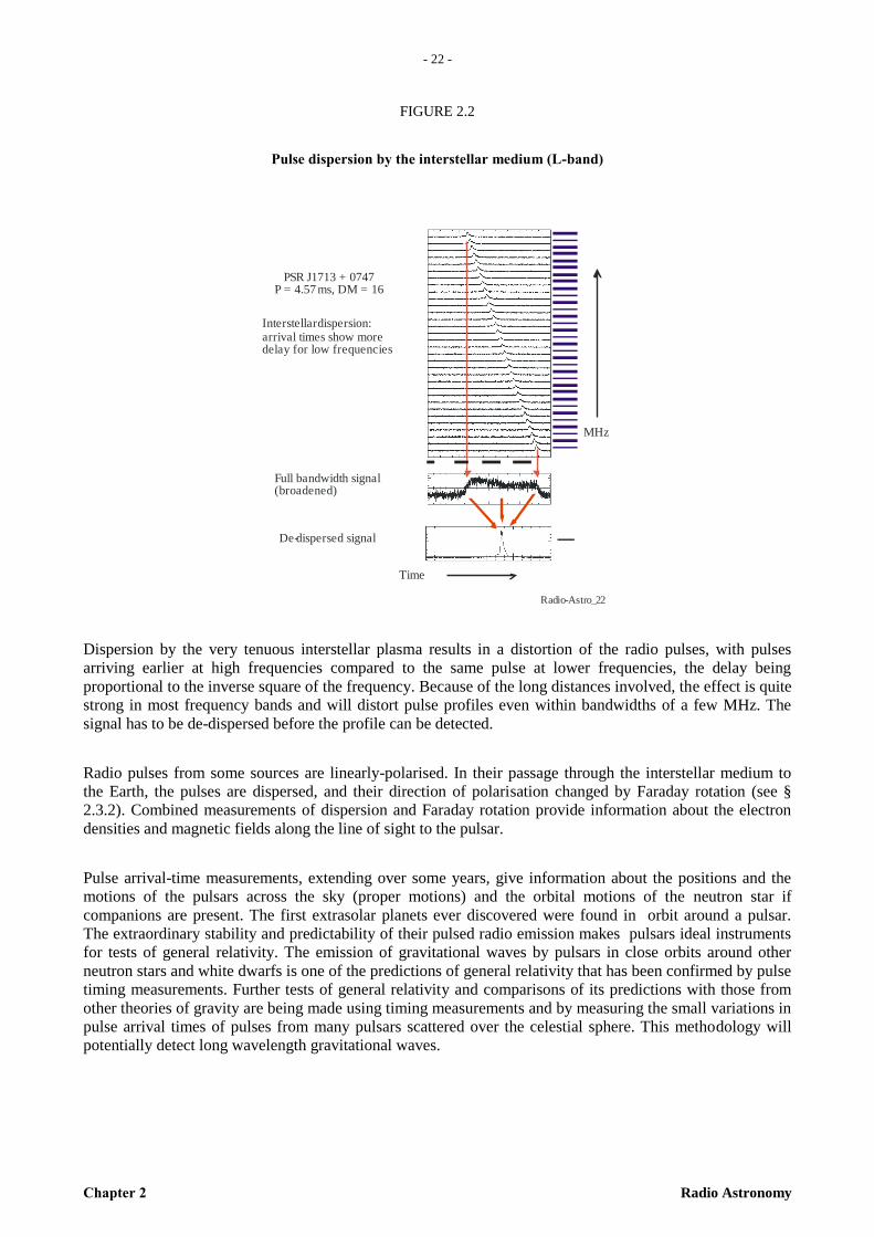
- 22 -
Chapter 2 Radio Astronomy
FIGURE 2.2
Pulse dispersion by the interstellar medium (L-band)
Radio-Astro_22
PSR J1713 + 0747ms, DM = 16P = 4.57
Interstellar dispersion:arrival times show moredelay for low frequencies
Full bandwidth signal(broadened)
De-dispersed signal
MHz
Time
Dispersion by the very tenuous interstellar plasma results in a distortion of the radio pulses, with pulses
arriving earlier at high frequencies compared to the same pulse at lower frequencies, the delay being
proportional to the inverse square of the frequency. Because of the long distances involved, the effect is quite
strong in most frequency bands and will distort pulse profiles even within bandwidths of a few MHz. The
signal has to be de-dispersed before the profile can be detected.
Radio pulses from some sources are linearly-polarised. In their passage through the interstellar medium to
the Earth, the pulses are dispersed, and their direction of polarisation changed by Faraday rotation (see §
2.3.2). Combined measurements of dispersion and Faraday rotation provide information about the electron
densities and magnetic fields along the line of sight to the pulsar.
Pulse arrival-time measurements, extending over some years, give information about the positions and the
motions of the pulsars across the sky (proper motions) and the orbital motions of the neutron star if
companions are present. The first extrasolar planets ever discovered were found in orbit around a pulsar.
The extraordinary stability and predictability of their pulsed radio emission makes pulsars ideal instruments
for tests of general relativity. The emission of gravitational waves by pulsars in close orbits around other
neutron stars and white dwarfs is one of the predictions of general relativity that has been confirmed by pulse
timing measurements. Further tests of general relativity and comparisons of its predictions with those from
other theories of gravity are being made using timing measurements and by measuring the small variations in
pulse arrival times of pulses from many pulsars scattered over the celestial sphere. This methodology will
potentially detect long wavelength gravitational waves.
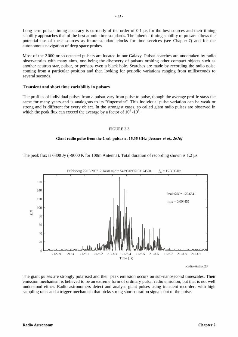
- 23 -
Radio Astronomy Chapter 2
– 2
3 –
Long-term pulsar timing accuracy is currently of the order of 0.1 µs for the best sources and their timing
stability approaches that of the best atomic time standards. The inherent timing stability of pulsars allows the
potential use of these sources as future standard clocks for time services (see Chapter 7) and for the
autonomous navigation of deep space probes.
Most of the 2 000 or so detected pulsars are located in our Galaxy. Pulsar searches are undertaken by radio
observatories with many aims, one being the discovery of pulsars orbiting other compact objects such as
another neutron star, pulsar, or perhaps even a black hole. Searches are made by recording the radio noise
coming from a particular position and then looking for periodic variations ranging from milliseconds to
several seconds.
Transient and short time variability in pulsars
The profiles of individual pulses from a pulsar vary from pulse to pulse, though the average profile stays the
same for many years and is analogous to its "fingerprint". This individual pulse variation can be weak or
strong and is different for every object. In the strongest cases, so called giant radio pulses are observed in
which the peak flux can exceed the average by a factor of 106 -10
8.
FIGURE 2.3
Giant radio pulse from the Crab pulsar at 15.35 GHz [Jessner et al., 2010]
The peak flux is 6800 Jy (~9000 K for 100m Antenna). Total duration of recording shown is 1.2 µs
Radio-Astro_23
2122.9 2123 2123.1 2123.2 2123.3 2123.4 2123.5 2123.6 2123.7 2123.8 2123.90
20
40
60
80
100
120
140
160
Time (ms)
Effelsberg 25/10/2007 2:14:40 mjd = 54398.0935193174520 fsky = 15.35 GHz
Peak / = 170.6541S N
rms = 0.004455
SN/
The giant pulses are strongly polarised and their peak emission occurs on sub-nanosecond timescales. Their
emission mechanism is believed to be an extreme form of ordinary pulsar radio emission, but that is not well
understood either. Radio astronomers detect and analyse giant pulses using transient recorders with high
sampling rates and a trigger mechanism that picks strong short-duration signals out of the noise.

- 24 -
Chapter 2 Radio Astronomy
Not all pulses that pulsars emit can be detected all the time. Interstellar scintillations (similar to the twinkling
of stars on the night sky, but caused by variability of the interstellar medium) modulates their radio emission
and, being a plasma effect, is again strongly frequency dependent. Pulsar scintillations are studied in order
to understand more about the structure and density distribution of electrons in the interstellar medium on a
variety of different length scales.
Some pulsars, however, emit their radiation quite irregularly. Some of these objects miss a few pulses
(nulling) from time to time, but in some cases, the pulsar is quiet for many days before suddenly restarting its
emissions. An extreme case of this behaviour is observed from the rotating radio transients (RRATS) which
are strong emitters, but with random outbursts lasting only a few seconds, and detectable maybe only once or
twice a day. Their detection and analysis requires a large antenna operating in a radio band which is free of
sporadic pulsed interference.
2.3.2 Measurement of continuum radiation
Measurements are required at a number of frequencies to establish the frequency dependence of continuum
emission. It suffices to make these at approximately octave intervals as the spectrum of continuum emission
is usually smooth, though more closely spaced intervals are desirable for the measurement of pulsar
dispersion, Faraday rotation, as well as for self-absorption spectra. The sensitivity of a measurement is
increased by the use of large fractional bandwidths at each frequency, where 10% is desirable, and 2% is
considered to be the minimum. RAS bands allocated for continuum measurements are discussed in
Chapter 3.
Most observations of radio sources at frequencies greater than about 100 MHz are made using parabolic-
reflector antennas, “dishes”. These may be used singly or in arrays. The limiting factor in the use of single-
dish radio telescopes is their angular resolution, which corresponds to their half-power beamwidth. They can
only effectively map structure in the sky that subtends angles of at least several antenna beamwidths: for
example, the radio emission from the Milky Way, the Sun, the Moon, and from some nearby galaxies. The
usual procedure is to divide the area to be mapped into a series of raster scans, separated by no more than
half the beamwidth, or into a grid of points with a spacing of no more than half the beamwidth. It can take a
long time to make a map, with the implicit assumption that the source and the environment in which the
measurements are made do not change during this time. In general, the measurement procedure is arranged
so that during a scan the point of observation is at a constant elevation. Whereupon the effect of ground
radiation in the side-lobes remains constant during a scan and is more easily removed. However, in many
cases, single-dish telescopes have beamwidths wider than the source being observed. In such cases the
measurements consist of a determination of the properties (e.g. intensity, polari”sation) of radiation from the
direction of the source under investigation, as compared with those of radiation from nearby regions of sky.
Ideally, a map is made of the area around and including the source, so that the excess emission over the
background can be estimated. However, when time does not permit this, measurements on and bracketing the
source are made as illustrated in Figure 2.4. In most cases the measured properties do not change
significantly over the duration of the observation, and can be averaged over time for each direction in the
sky. The variations in receiver output on a short time scale are illustrated in Figure 2.5. The contribution
from the source to the total radiation received is estimated as S – (A B C D)/4, where the letters
represent the averaged power levels received at the corresponding pointing directions in Figure 2.4.
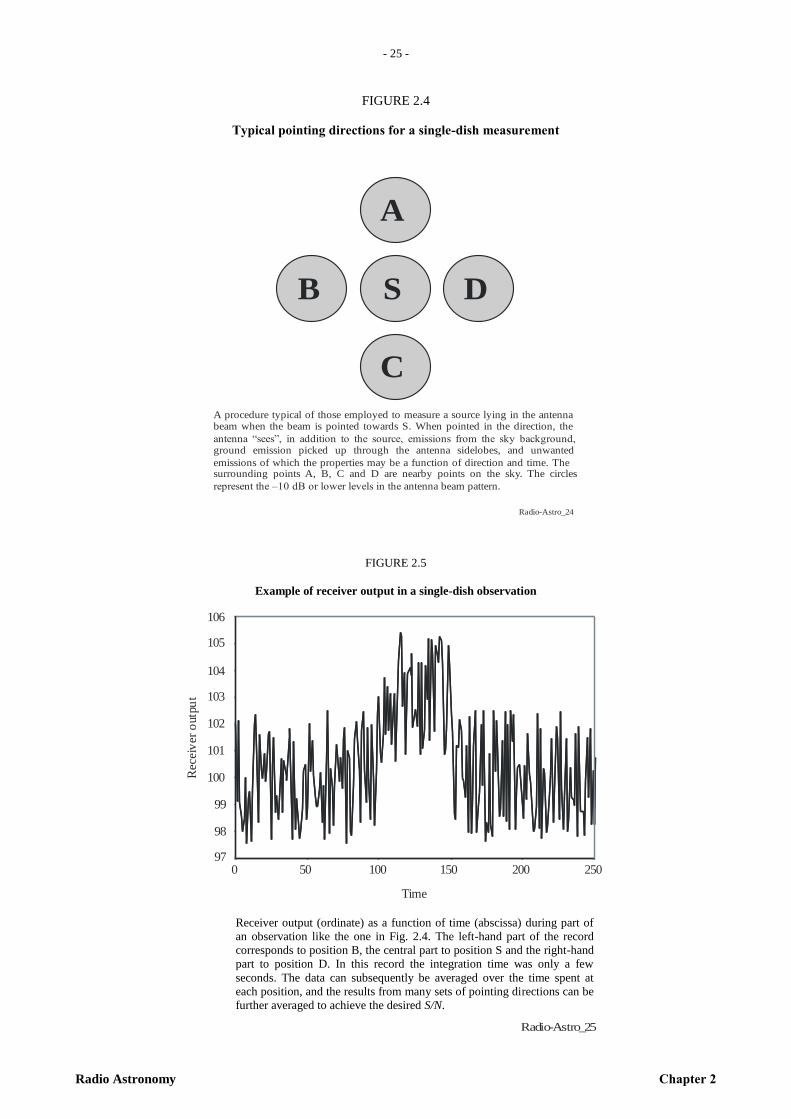
- 25 -
Radio Astronomy Chapter 2
– 2
5 –
FIGURE 2.4
Typical pointing directions for a single-dish measurement
Radio-Astro_24
A procedure typical of those employed to measure a source lying in the antenna beam when the beam is pointed towards S. When pointed in the direction, the
antenna “sees”, in addition to the source, emissions from the sky background, ground emission picked up through the antenna sidelobes, and unwanted
emissions of which the properties may be a function of direction and time. The surrounding points A, B, C and D are nearby points on the sky. The circles
represent the –10 dB or lower levels in the antenna beam pattern.
B S D
C
A
FIGURE 2.5
Example of receiver output in a single-dish observation
Time
Rec
eiv
er o
utpu
t
0 10097
100
106
50 150 200 250
98
99
101
102
103
104
105
Radio-Astro_25
Receiver output (ordinate) as a function of time (abscissa) during part of
an observation like the one in Fig. 2.4. The left-hand part of the record
corresponds to position B, the central part to position S and the right-hand
part to position D. In this record the integration time was only a few
seconds. The data can subsequently be averaged over the time spent at
each position, and the results from many sets of pointing directions can be
further averaged to achieve the desired S/N.
Radio-Astro_25
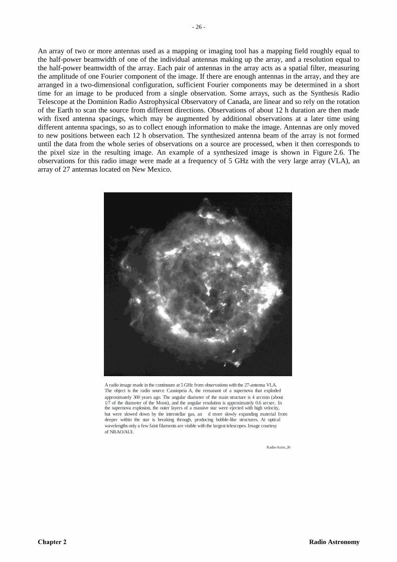
- 26 -
Chapter 2 Radio Astronomy
An array of two or more antennas used as a mapping or imaging tool has a mapping field roughly equal to
the half-power beamwidth of one of the individual antennas making up the array, and a resolution equal to
the half-power beamwidth of the array. Each pair of antennas in the array acts as a spatial filter, measuring
the amplitude of one Fourier component of the image. If there are enough antennas in the array, and they are
arranged in a two-dimensional configuration, sufficient Fourier components may be determined in a short
time for an image to be produced from a single observation. Some arrays, such as the Synthesis Radio
Telescope at the Dominion Radio Astrophysical Observatory of Canada, are linear and so rely on the rotation
of the Earth to scan the source from different directions. Observations of about 12 h duration are then made
with fixed antenna spacings, which may be augmented by additional observations at a later time using
different antenna spacings, so as to collect enough information to make the image. Antennas are only moved
to new positions between each 12 h observation. The synthesized antenna beam of the array is not formed
until the data from the whole series of observations on a source are processed, when it then corresponds to
the pixel size in the resulting image. An example of a synthesized image is shown in Figure 2.6. The
observations for this radio image were made at a frequency of 5 GHz with the very large array (VLA), an
array of 27 antennas located on New Mexico.
A radio image made in the continuum at 5 GHz from observations with the 27-antenna VLA. The object is the radio source Cassiopeia A, the remanant of a supernova that exploded
approximately 300 years ago. The angular diameter of the main structure is 4 arcmin (about 1/7 of the diameter of the Moon), and the angular resolution is approximately 0.6 arcsec. In the supernova explosion, the outer layers of a massive star were ejected with high velocity,
but were slowed down by the interstellar gas, an d more slowly expanding material from deeper within the star is breaking through, producing bubble-like structures. At optical
wavelengths only a few faint filaments are visible with the largest telescopes. Image courtesy
of NRAO/AUI.
Radio-Astro_26
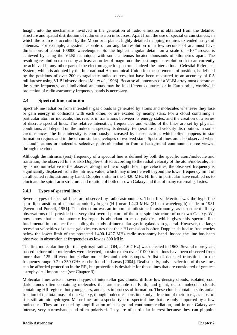
- 27 -
Radio Astronomy Chapter 2
– 2
7 –
Insight into the mechanisms involved in the generation of radio emission is obtained from the detailed
structure and spatial distribution of radio emission in sources. Apart from the use of special circumstances, in
which the source is occulted by the Moon or a planet, highly detailed mapping requires extended arrays of
antennas. For example, a system capable of an angular resolution of a few seconds of arc must have
dimensions of about 100000 wavelengths. So the highest angular detail, on a scale of ~10–4
arcsec, is
achieved by using the VLBI technique, with some antennas located thousands of kilometres apart. The
resulting resolution exceeds by at least an order of magnitude the best angular resolution that can currently
be achieved in any other part of the electromagnetic spectrum. Indeed the International Celestial Reference
System, which is adopted by the International Astronomical Union for measurements of position, is defined
by the positions of over 200 extragalactic radio sources that have been measured to an accuracy of 0.5
milliarcsec using VLBI observations [Ma et al., 1998]. Because all antennas of a VLBI array must operate at
the same frequency, and individual antennas may be in different countries or in Earth orbit, worldwide
protection of radio astronomy frequency bands is necessary.
2.4 Spectral-line radiation
Spectral-line radiation from interstellar gas clouds is generated by atoms and molecules whenever they lose
or gain energy in collisions with each other, or are excited by nearby stars. For a cloud containing a
particular atom or molecule, this results in transitions between its energy states, and the creation of a series
of discrete spectral lines. The relative intensities, frequencies and widths of the lines are set by physical
conditions, and depend on the molecular species, its density, temperature and velocity distribution. In some
circumstances, the line intensity is enormously increased by maser action, which often happens in star
formation regions and in the circumstellar envelopes of evolved stars. Spectral lines are also observed when
a cloud’s atoms or molecules selectively absorb radiation from a background continuum source viewed
through the cloud.
Although the intrinsic (rest) frequency of a spectral line is defined by both the specific atom/molecule and
transition, the observed line is also Doppler-shifted according to the radial velocity of the atom/molecule, i.e.
by its motion relative to the observer along the line of sight. For large velocities, the observed frequency is
significantly displaced from the intrinsic value, which may often lie well beyond the lower frequency limit of
an allocated radio astronomy band. Doppler shifts in the 1 420 MHz HI line in particular have enabled us to
elucidate the spiral-arm structure and rotation of both our own Galaxy and that of many external galaxies.
2.4.1 Types of spectral lines
Several types of spectral lines are observed by radio astronomers. Their first detection was the hyperfine
spin-flip transition of neutral atomic hydrogen (HI) near 1 420 MHz (21 cm wavelength) made in 1951
[Ewen and Purcell, 1951]. This detection was an important milestone in astronomy, as subsequent all-sky
observations of it provided the very first overall picture of the true spiral structure of our own Galaxy. We
now know that neutral atomic hydrogen is abundant in most galaxies, which gives this spectral line
fundamental importance for enabling the study of interstellar gas in galaxies in general. However, the large
recession velocities of distant galaxies ensures that their HI emission is often Doppler-shifted to frequencies
below the lower limit of the protected 1 400-1 427 MHz radio astronomy band. Indeed the line has been
observed in absorption at frequencies as low as 300 MHz.
The first molecular line (for the hydroxyl radical, OH, at 1.6 GHz) was detected in 1963. Several more years
passed before other molecules were detected, but since then over 10 000 transitions have been observed from
more than 125 different interstellar molecules and their isotopes. A list of detected transitions in the
frequency range 0.7 to 350 GHz can be found in Lovas [2004]. Realistically, only a selection of these lines
can be afforded protection in the RR, but protection is desirable for those lines that are considered of greatest
astrophysical importance (see Chapter 3).
Molecular lines arise in several types of interstellar gas clouds: diffuse low-density clouds; isolated, cool
dark clouds often containing molecules that are unstable on Earth; and giant, dense molecular clouds
containing HII regions, hot young stars, and stars in process of formation. These clouds contain a substantial
fraction of the total mass of our Galaxy, though molecules constitute only a fraction of their mass, as most of
it is still atomic hydrogen. Maser lines are a special type of spectral line that are only supported by a few
molecules. They are created by amplification of background continuum radiation, and in our Galaxy are
intense, very narrowband, and often polarised. They are of particular interest because they can pinpoint
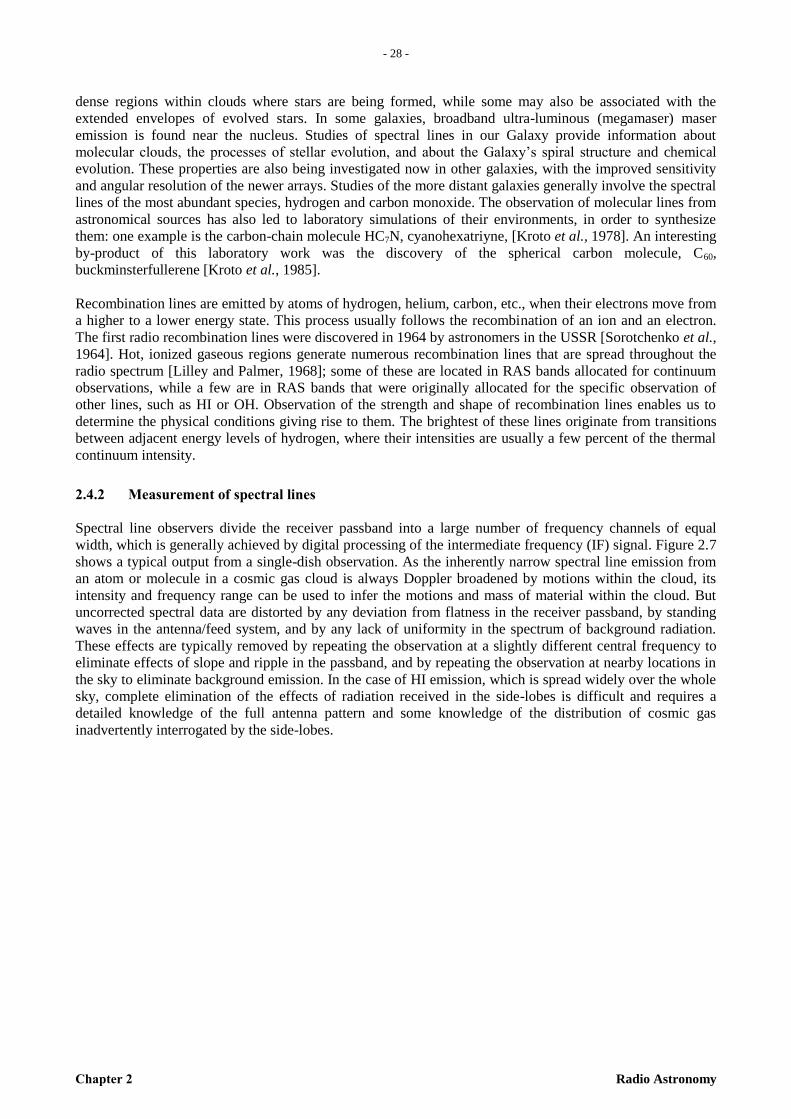
- 28 -
Chapter 2 Radio Astronomy
dense regions within clouds where stars are being formed, while some may also be associated with the
extended envelopes of evolved stars. In some galaxies, broadband ultra-luminous (megamaser) maser
emission is found near the nucleus. Studies of spectral lines in our Galaxy provide information about
molecular clouds, the processes of stellar evolution, and about the Galaxy’s spiral structure and chemical
evolution. These properties are also being investigated now in other galaxies, with the improved sensitivity
and angular resolution of the newer arrays. Studies of the more distant galaxies generally involve the spectral
lines of the most abundant species, hydrogen and carbon monoxide. The observation of molecular lines from
astronomical sources has also led to laboratory simulations of their environments, in order to synthesize
them: one example is the carbon-chain molecule HC7N, cyanohexatriyne, [Kroto et al., 1978]. An interesting
by-product of this laboratory work was the discovery of the spherical carbon molecule, C60,
buckminsterfullerene [Kroto et al., 1985].
Recombination lines are emitted by atoms of hydrogen, helium, carbon, etc., when their electrons move from
a higher to a lower energy state. This process usually follows the recombination of an ion and an electron.
The first radio recombination lines were discovered in 1964 by astronomers in the USSR [Sorotchenko et al.,
1964]. Hot, ionized gaseous regions generate numerous recombination lines that are spread throughout the
radio spectrum [Lilley and Palmer, 1968]; some of these are located in RAS bands allocated for continuum
observations, while a few are in RAS bands that were originally allocated for the specific observation of
other lines, such as HI or OH. Observation of the strength and shape of recombination lines enables us to
determine the physical conditions giving rise to them. The brightest of these lines originate from transitions
between adjacent energy levels of hydrogen, where their intensities are usually a few percent of the thermal
continuum intensity.
2.4.2 Measurement of spectral lines
Spectral line observers divide the receiver passband into a large number of frequency channels of equal
width, which is generally achieved by digital processing of the intermediate frequency (IF) signal. Figure 2.7
shows a typical output from a single-dish observation. As the inherently narrow spectral line emission from
an atom or molecule in a cosmic gas cloud is always Doppler broadened by motions within the cloud, its
intensity and frequency range can be used to infer the motions and mass of material within the cloud. But
uncorrected spectral data are distorted by any deviation from flatness in the receiver passband, by standing
waves in the antenna/feed system, and by any lack of uniformity in the spectrum of background radiation.
These effects are typically removed by repeating the observation at a slightly different central frequency to
eliminate effects of slope and ripple in the passband, and by repeating the observation at nearby locations in
the sky to eliminate background emission. In the case of HI emission, which is spread widely over the whole
sky, complete elimination of the effects of radiation received in the side-lobes is difficult and requires a
detailed knowledge of the full antenna pattern and some knowledge of the distribution of cosmic gas
inadvertently interrogated by the side-lobes.
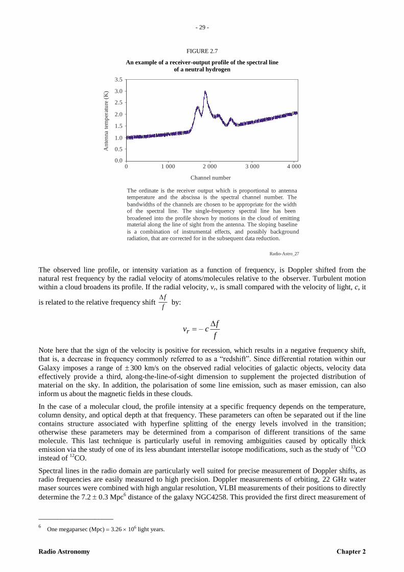
- 29 -
Radio Astronomy Chapter 2
– 2
9 –
FIGURE 2.7
An example of a receiver-output profile of the spectral line
of a neutral hydrogen
Channel number
An
ten
na t
emp
erat
ure
(K
)
0.0
1.5
0.5
1.0
2.0
2.5
3.0
3.5
The ordinate is the receiver output which is proportional to antenna temperature and the abscissa is the spectral channel number. The
bandwidths of the channels are chosen to be appropriate for the width of the spectral line. The single-frequency spectral line has been
broadened into the profile shown by motions in the cloud of emitting material along the line of sight from the antenna. The sloping baseline
is a combination of instrumental effects, and possibly background radiation, that are corrected for in the subsequent data reduction.
0 1 000 2 000 3 000 4 000
Radio-Astro_27
The observed line profile, or intensity variation as a function of frequency, is Doppler shifted from the
natural rest frequency by the radial velocity of atoms/molecules relative to the observer. Turbulent motion
within a cloud broadens its profile. If the radial velocity, vr, is small compared with the velocity of light, c, it
is related to the relative frequency shift by:
Note here that the sign of the velocity is positive for recession, which results in a negative frequency shift,
that is, a decrease in frequency commonly referred to as a “redshift”. Since differential rotation within our
Galaxy imposes a range of 300 km/s on the observed radial velocities of galactic objects, velocity data
effectively provide a third, along-the-line-of-sight dimension to supplement the projected distribution of
material on the sky. In addition, the polarisation of some line emission, such as maser emission, can also
inform us about the magnetic fields in these clouds.
In the case of a molecular cloud, the profile intensity at a specific frequency depends on the temperature,
column density, and optical depth at that frequency. These parameters can often be separated out if the line
contains structure associated with hyperfine splitting of the energy levels involved in the transition;
otherwise these parameters may be determined from a comparison of different transitions of the same
molecule. This last technique is particularly useful in removing ambiguities caused by optically thick
emission via the study of one of its less abundant interstellar isotope modifications, such as the study of 13
CO
instead of 12
CO.
Spectral lines in the radio domain are particularly well suited for precise measurement of Doppler shifts, as
radio frequencies are easily measured to high precision. Doppler measurements of orbiting, 22 GHz water
maser sources were combined with high angular resolution, VLBI measurements of their positions to directly
determine the 7.2 0.3 Mpc6 distance of the galaxy NGC4258. This provided the first direct measurement of
____________________
6 One megaparsec (Mpc) 3.26 106 light years.
f
f
f
fcvr
–
- 30 -
Chapter 2 Radio Astronomy
the distance to an extragalactic object that is entirely independent of any other sequence of astronomical
measurements [Herrnstein et al., 1999].
Every spectrometer channel corresponds to a particular Doppler shift range, so when an antenna array is used
for spectral line observations, a separate image is made for every channel. In many cases the Doppler shift
can be interpreted as a distance, and instead of a data map one gets a data cube, which is a representation of
the distribution of the source material in a cube of space.
Many hours of observation are often required to obtain the sensitivities necessary to form conclusions of
astrophysical interest. An absence of harmful interference is necessary over bandwidths broad enough to
include both the Doppler-shifted lines and the comparison bands bordering the line emission.
2.5 Modern Practice
Radio astronomers benefit from many technical developments. These are progressively increasing the central
frequencies of practical receivers, as well as decreasing their system temperature and increasing their
bandwidth. Digital backends are now universal, with data acquisition under computer control. This facilitates
making short integrations, whose output can be inspected for severe RFI before being averaged to obtain the
desired sensitivity. Advances in data throughput, and the ever more affordable cost of memory, enable large
datasets to be saved for later processing by ever more sophisticated algorithms. One of the biggest
beneficiaries of many of these advances are astronomers who make VLBI observations. They can now
simultaneously use telescopes located in both North & South America, as well as in Europe and South
Africa, to obtain data in real time over fibre networks, reduce the data and obtain the resulting images in
almost real time. The bandwidth of this class of observation has doubled several times in the last decade,
with consequent gains in sensitivity. By contrast, VLBI observations were previously stored to magnetic
tape, to be reduced in the following months: single-dish spectral-line observers have not had to endure such a
slow cadence since the 1960s.
Technical advances have changed the prefered mode for making continuum observations: it is now usually
better to deploy a digital spectrometer that allows severe RFI to be identified and removed from spectra
before getting a continuum measurement. Likewise, the larger bandwidths of current receivers has
encouraged those observers fortunate enough to have observing modes with some inherent protection against
RFI to observe outside the allocated RAS bands. Other observers obtain astronomically valid data by using
notch filters (sometimes of the high-temperature super-conducting type) to suppress intense unwanted
signals adjacent to their chosen bandpass, as well as by using high spectral resolution to enable excision
techniques to be applied to anthropic narrow-band features. Nevertheless, the RAS still needs its allocated
bands, both to enable accurate calibration of data, and to minimize RFI-related ambiguity in spectral line
observations.
2.6 Conclusion
Radio astronomy has an essential role in the investigation of the fundamental physics and astronomy of the
Universe. Many of the studied phenomena are not observable in other parts of the electromagnetic spectrum,
as occurs for example for the line emission from neutral atomic hydrogen, the microwave background
emission and its angular structure that is of fundamental importance in cosmology, the large regions of
synchrotron emission associated with radio galaxies, and the regions of star formation obscured by dust at
optical wavelengths, to mention just a few. Moreover, the radio domain provides us with the highest
achievable angular resolution, and the most precise angular positions, as well as the most accurate Doppler
shifts. Thus radio astronomy, rather than being a simple adjunct to traditional optical techniques, plays a
leading discovery role in many areas of astronomy and astrophysics.

- 31 -
Radio Astronomy Chapter 2
– 3
1 –
REFERENCES
BENNET, C. et al. [2003] "The Microwave Anisotropy Probe (MAP) Mission", Astrophysical Journal,
Vol 583 (1), p. 1–23.
BURKE, B. F. and GRAHAM-SMITH, F. [2002] An introduction to radio astronomy, 2nd ed., Cambridge
University Press.
EWEN, H. I. and PURCELL, E. M. [1951] Observations of a line in the galactic radio spectrum. Nature,
Vol. 168, p. 356.
HERRNSTEIN, J. R., MORAN, J. M., GREENHILL, L. J., DIAMOND, P. J., INOUE, M., NAKAI, N.,
MITOSHI, M., HENKEL, C. and RIESS, A. [1999] A geometric distance to the galaxy NGC4258 from
orbital motions in a nuclear gas disk. Nature, Vol. 158, p. 539.
HEWISH, A., BELL, S. J., PILKINGTON, J. D. H., SCOTT, P. F. and COLLINS, R. A. [1968]
Observations of a rapidly pulsating radio source. Nature, Vol. 217, p. 709-713.
JANSKY, K. G. [1935] A note on the source of interstellar interference. Proc. IRE. Vol. 23, p. 1158-1163.
JESSNER, A. et al. [2010] Giant pulses with nanosecond time resolution detected from the Crab pulsar at
8.5 and 15.1 GHz, Astronomy and Astrophysics, Vol. 524, id.A60
KROTO, H. W., KIRBY, C., WALTON, D. R. M., AVERY, L. W., BROTEN, N. W., MACLEOD, J. M.
and OKA, T. [1978] The detection of cyanohexatriyne in Heiles’s cloud 2. Astrophys. J.,
Vol. 219, L133-L137.
KROTO, H. W., HEATH, J. R., OBRIEN, S. C., CURL, R. F. and SMALLEY, R. E. [1985] C60:
Buckminsterfullerine. Nature, Vol. 318, p. 162-163.
LILLEY, A. E. and PALMER, P. [1968] Tables of radio frequency recombination lines. Astrophys. J., Suppl.
Series, Vol. 16, p. 143-174.
D. LORIMER, D. and KRAMER, M [2005]: Handbook of Pulsar Astronomy, CUP, Cambridge (U.K.).
LOVAS, F. J. [2004] Recommended rest frequencies for observed interstellar molecular microwave
transitions – 2002 revision. J. Phys. and Chem. Ref. Data. Vol. 33, p. 117-335.
MA, C, ARIAS, E. F., FEY, A. L., GONTIER, A.-M., JACOBS, C. S., SOVERS, O. J., ARCHINAL, B. A.
and CHARLOT, P. [1998] The international celestial reference frame as realized by very long baseline
interferometry. Astron. J., Vol. 116, p. 516-546.
MCLEAN, D. J. and LABRUM, N. R. [1985] Studies of the sun at metre wavelengths. Cambridge University
Press.
Planck Collaboration et. al [2011] Planck early results. I. The Planck Mission, Astron. and Astrophys, Vol.
536, 1
PRYKE, C., HALVERSON, N. W., LEITCH, E. M., KOVAC, J., CARLSTROM, J. E., HOLZAPFEL, W.
L. and DRAGOVAN, N. [2002] Cosmological parameter extraction from the first season of observations
with the degree angular scale interferometer. Astrophys. J., Vol. 568, p. 46-51.
ROBERTS, J. A. [1963] Radio emission from the planets. Planet and Space Sci., Vol. 11, p. 221.
SMOOT, G. F. and 27 co-authors [1992] Structure of the COBE differential microwave radiometer first-year
maps. Astrophys. J., Vol. 396, L1-L5.
SOROTCHENKO, R. L., BORODZITCH, O. S., DRAVSKIKH, Z. V. and KOLBASSOV, V. A. [1964]
Proc. of the XIIth General Assembly of the International Astronomical Union, Hamburg, Germany.
- 32 -
Chapter 3 Radio Astronomy
CHAPTER 3
Preferred frequency bands for radio astronomy observations
3.1 General considerations
3.1.1 Ground-based radio astronomy observations
The choice of frequency for ground-based radio astronomy observations depends on the phenomena to be
observed and the Earth’s atmosphere (troposphere and ionosphere). The ionosphere strongly affects
observations at frequencies below 30 MHz; measurements suggest that the lowest practicable frequency for
ground-based observation is about 1.5 MHz (see § 3.2.1); most observations are carried out at frequencies
above about 20 MHz. The troposphere affects observations by absorption, primarily by oxygen (O2) and
water vapour (H2O). Attenuation due to resonances of these molecules is shown schematically in Figure 3.1.
The effects of other atmospheric constituents, for example CO, NO, and NO2, are negligible. Although some
of the first discoveries of galactic radio emission were made at some tens of megahertz (i.e. decametre
wavelengths), there has been a general progression in radio astronomy to measurements at higher
frequencies.
The high angular resolution attainable with parabolic antennas, the development of low-noise
pre-amplifiers, and the succession of discoveries at the higher frequencies, have contributed to that trend.
Radio astronomers have pioneered the use of frequencies above 100 GHz, and observations are now being
made at frequencies as high as 1 000 GHz. The Atacama Large Millimeter submillimeter Array (ALMA)
started its operations in 20107. ALMA is located in the Atacama desert, Chile, and can observe in a
frequency range between 30 and 950 GHz, with a spatial resolution of up to 0.01 seconds of arc. ALMA is
expected to reveal the detailed structure of planet formation sites, formation and evolution of galaxies, the
relation between the Universe and Origin of Life, and other frontiers in astronomy.
Aside from the new results at high frequencies, there are phenomena of astrophysical interest that occur only
at the lower frequencies, for example, free-free absorption in ionized regions of the Galaxy, self-absorption
in extra-galactic radio sources, and low-frequency emission mechanisms from tenuous plasmas in clusters of
galaxies.
____________________
7 http://www.almaobservatory.org/

- 33 -
Radio Astronomy Chapter 3
– 3
3 –
FIGURE 3.1
Atmospheric attenuation computed over horizontal paths of 1 km at four different altitudes.
For reference, free-space loss over 1 km is also plotted.
Radio-Astro_31
01
10
Frequency (GHz)
1 000 m altitude
Att
enu
atio
n (
dB
/km
)
500 1 000 1 500 2 000 2 500 3 000
1 000 000
100 000
10 000
1 000
100
0 m altitude
3 000 m altitude
Free space loss over 1 km
3.1.2 Space-based radio astronomy observations
Space-based observation is a rather new field for radio astronomy. Several space-based radio astronomy
observations were performed by, for example, COBE, SWAS, ODIN HALCA, WMAP and PLANCK.
The COBE, WMAP and PLANCK satellites detected and mapped the anisotropy of the cosmic microwave
background radiation. The distribution of the cosmic microwave background radiation measured between 30
and 857 GHz by the PLANCK (see Figure 3.2) resulted in determining the age of the Universe to be 13.8
billion years and in deriving the remarkable fact: ordinary atoms (also called baryons) make up only 4.9% of
the Universe, dark matter (matter not made up of atoms) is 26.8%, and dark energy, in the form of a
cosmological constant, makes up 68.3% of the Universe, causing the expansion rate of the Universe to
speed up.
SWAS and ODIN observed frequencies higher than 100 GHz and up to about 500 GHz, to measure
abundances of H2O, O2 and other spectral lines that are almost impossible to observe from
the Earth’s surface.
The HALCA satellite was combined with ground-based radio telescopes to make the first space-VLBI
experiments at 1.4, 1.6 and 5 GHz. Because there is no atmospheric absorption, space-based radio astronomy
is very important for observing in frequency ranges where ground-based observations cannot be made.
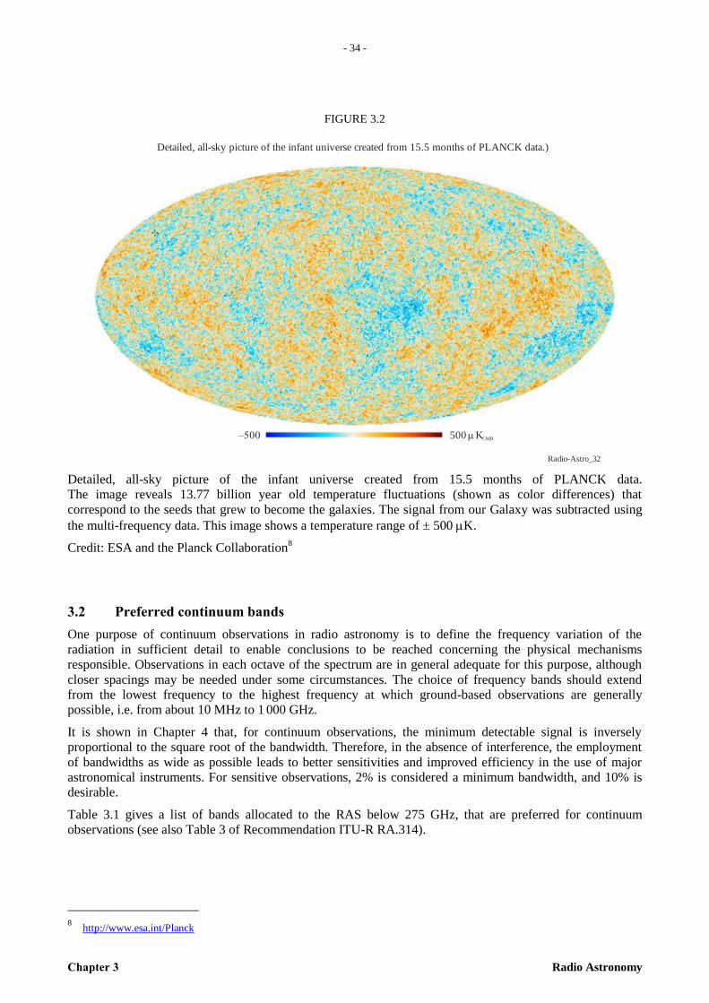
- 34 -
Chapter 3 Radio Astronomy
FIGURE 3.2
Radio-Astro_32
–500 500 Km CMB
Detailed, all-sky picture of the infant universe created from 15.5 months of PLANCK data.)
Detailed, all-sky picture of the infant universe created from 15.5 months of PLANCK data.
The image reveals 13.77 billion year old temperature fluctuations (shown as color differences) that
correspond to the seeds that grew to become the galaxies. The signal from our Galaxy was subtracted using
the multi-frequency data. This image shows a temperature range of ± 500 mK.
Credit: ESA and the Planck Collaboration8
3.2 Preferred continuum bands
One purpose of continuum observations in radio astronomy is to define the frequency variation of the
radiation in sufficient detail to enable conclusions to be reached concerning the physical mechanisms
responsible. Observations in each octave of the spectrum are in general adequate for this purpose, although
closer spacings may be needed under some circumstances. The choice of frequency bands should extend
from the lowest frequency to the highest frequency at which ground-based observations are generally
possible, i.e. from about 10 MHz to 1 000 GHz.
It is shown in Chapter 4 that, for continuum observations, the minimum detectable signal is inversely
proportional to the square root of the bandwidth. Therefore, in the absence of interference, the employment
of bandwidths as wide as possible leads to better sensitivities and improved efficiency in the use of major
astronomical instruments. For sensitive observations, 2% is considered a minimum bandwidth, and 10% is
desirable.
Table 3.1 gives a list of bands allocated to the RAS below 275 GHz, that are preferred for continuum
observations (see also Table 3 of Recommendation ITU-R RA.314).
____________________
8 http://www.esa.int/Planck
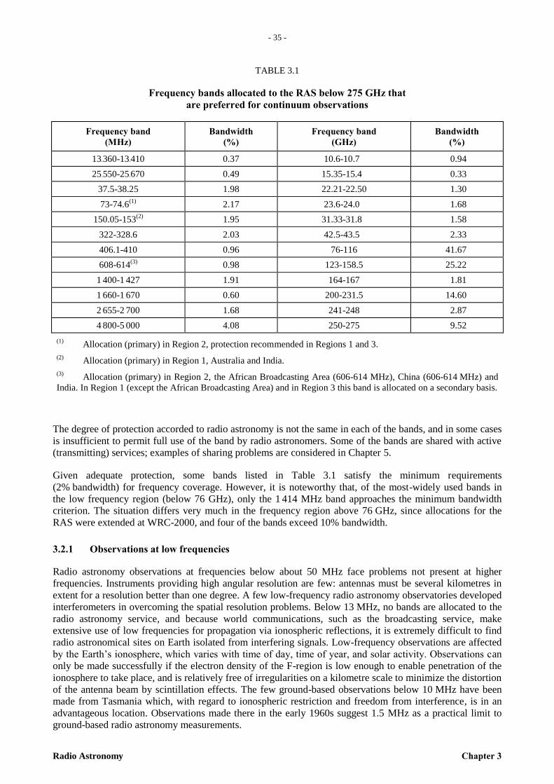
- 35 -
Radio Astronomy Chapter 3
– 3
5 –
TABLE 3.1
Frequency bands allocated to the RAS below 275 GHz that
are preferred for continuum observations
The degree of protection accorded to radio astronomy is not the same in each of the bands, and in some cases
is insufficient to permit full use of the band by radio astronomers. Some of the bands are shared with active
(transmitting) services; examples of sharing problems are considered in Chapter 5.
Given adequate protection, some bands listed in Table 3.1 satisfy the minimum requirements
(2% bandwidth) for frequency coverage. However, it is noteworthy that, of the most-widely used bands in
the low frequency region (below 76 GHz), only the 1 414 MHz band approaches the minimum bandwidth
criterion. The situation differs very much in the frequency region above 76 GHz, since allocations for the
RAS were extended at WRC-2000, and four of the bands exceed 10% bandwidth.
3.2.1 Observations at low frequencies
Radio astronomy observations at frequencies below about 50 MHz face problems not present at higher
frequencies. Instruments providing high angular resolution are few: antennas must be several kilometres in
extent for a resolution better than one degree. A few low-frequency radio astronomy observatories developed
interferometers in overcoming the spatial resolution problems. Below 13 MHz, no bands are allocated to the
radio astronomy service, and because world communications, such as the broadcasting service, make
extensive use of low frequencies for propagation via ionospheric reflections, it is extremely difficult to find
radio astronomical sites on Earth isolated from interfering signals. Low-frequency observations are affected
by the Earth’s ionosphere, which varies with time of day, time of year, and solar activity. Observations can
only be made successfully if the electron density of the F-region is low enough to enable penetration of the
ionosphere to take place, and is relatively free of irregularities on a kilometre scale to minimize the distortion
of the antenna beam by scintillation effects. The few ground-based observations below 10 MHz have been
made from Tasmania which, with regard to ionospheric restriction and freedom from interference, is in an
advantageous location. Observations made there in the early 1960s suggest 1.5 MHz as a practical limit to
ground-based radio astronomy measurements.
Frequency band
(MHz)
Bandwidth
(%)
Frequency band
(GHz)
Bandwidth
(%)
13.360-13.410 0.37 10.6-10.70 0.94
25.550-25.670 0.49 15.35-15.40 0.33
37.5-38.25 1.98 22.21-22.50 1.30
73-74.6(1)
2.17 23.6-24.00 1.68
150.05-153(2)
1.95 31.33-31.80 1.58
322-328.6 2.03 42.5-43.50 2.33
406.1-410 0.96 76-116 41.67
608-614(3)
0.98 123-158.5 25.22
1 400-1 427 1.91 164-167 1.81
1 660-1 670 0.60 200-231.5 14.60
2 655-2 700 1.68 241-248 2.87
4 800-5 000 4.08 250-275 9.52
(1) Allocation (primary) in Region 2, protection recommended in Regions 1 and 3.
(2) Allocation (primary) in Region 1, Australia and India.
(3) Allocation (primary) in Region 2, the African Broadcasting Area (606-614 MHz), China (606-614 MHz) and
India. In Region 1 (except the African Broadcasting Area) and in Region 3 this band is allocated on a secondary basis.
- 36 -
Chapter 3 Radio Astronomy
3.2.2 High frequency bands for continuum observations
At frequencies above 20 GHz the need to avoid the maxima in atmospheric absorption due to oxygen (O2)
and water vapour (H2O) dictates the choice of bands. Frequency bands for continuum observations must be
chosen to lie within the atmospheric absorption minima near 30, 90, 150, 240, 410, 470, 670 and 850 GHz.
Thus, despite the restriction of choice, adequate sampling intervals are available. Currently, radio astronomy
bands are allocated only up to a frequency of 275 GHz; an adopted policy of selection of bands containing
important spectral lines dictated the choice of frequency range for many of the bands, particularly at high
frequencies. It is noted that the bands 275-323 GHz, 327-371 GHz, 388-424 GHz, 426-442 GHz, 453-510
GHz, 623-711 GHz, 795-909 GHz and 926-945 GHz have been identified for use by administrations for the
radio astronomy service. In the 21st century, active services increasingly demand the use of higher frequency
bands for broadband communications. WRC-12 adopted the revised footnote 5.565, which states, “All
frequencies in the range 1 000-3 000 GHz may be used by both active and passive services”.
Report ITU-R RA.2189 reports study results on frequency sharing between 275 and 3 000 GHz. It concludes
that the sharing between radio astronomy and active services in the range 275-3 000 GHz is not problematic,
based on the following reasons:
On the ground, assuming nearly worst-case conditions, a terrestrial link in the 275-1 000 GHz range would
have to be at a high altitude running maximum available power through a large dish pointing directly at a
telescope to produce a signal at the telescope that may have a detrimental impact on radio astronomy
observing. Above 1 000 GHz, the interferer would have to be within 1 km distance running maximum power
and pointed directly at the telescope to exceed interference thresholds; most likely, such a closely-located
link would be under the control of the radio observatory itself, or would be subject to informal local
coordination with the affected observatory.
If considering interference from airborne transmitters, the small beamwidth of the interferer and the high
level of slant-path atmospheric attenuation would require that the plane fly directly over the radio telescope
to create interference. A single pass from a transmitter at 275 GHz and flying
7 000 m or more above the observatory would not exceed the Recommendation ITU-R RA.769 interference
level. Course deviations by the airplane of more than ~1/5 km could result in essentially no interference
being observed.
For interference by satellites, the competing factors of projected beam size, relative speed, and free space
loss combine to produce a relatively constant margin over the extrapolated Recommendation ITU-R RA.769
interference threshold levels. Assuming no additional losses due to atmospheric attenuation, and assuming
that the satellite passed directly over the telescope, the average signal level during a 2 000 s integration is
18 or more dB below the interference threshold. Even signal levels from geostationary satellites are not
expected to be sufficient to produce interference.
3.3 Bands for spectral-line observations
Spectral-line observations must be made at the specific frequencies set by the spectral emission of atoms or
molecules of interest. The lines that are considered of greatest astrophysical importance below 1000 GHz are
listed in the Tables 3.2 and 3.3 (see also Tables 1 and 2 of Recommendation ITU-R RA.314). In addition,
Recommendation ITU-R RA.1860 – Preferred frequency bands for radio astronomical measurements in the
range 1-3 THz, contains a very long list of spectral lines of greatest astrophysical importance between 1 000
and 3 000 GHz. These are based on a recommendation by the International Astronomical Union (IAU), and
selected from amongst the thousands of lines that have been detected or predicted in the microwave
spectrum9. The lists of most important lines are periodically updated by the IAU, and the revisions are
incorporated in the IAU Proceedings and also in Recommendations ITU-R RA.314 and RA.1860.
The bandwidths required for observations of the lines in Tables 3.2 and 3.3 are determined by Doppler
frequency shifts in the rest frequencies of the lines, caused by the radial velocity of the emitting region
relative to an observer on Earth. For most molecules, the velocity range is 300 km/s, to account for the
____________________
9 Splatalogue – Database for Astronomical Spectroscopy http://splatalogue.net/; the Cologne Database for Molecular Spectroscopy
http://www.astro.uni-koeln.de/cdms; NIST Recommended Rest Frequencies for Observed Interstellar Molecular Microwave
Transitions http://physics.nist.gov/cgi-bin/micro/table5/start.pl.
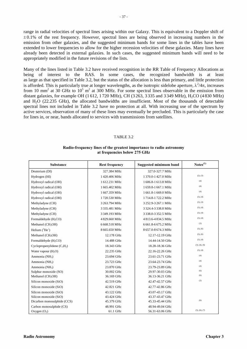
- 37 -
Radio Astronomy Chapter 3
– 3
7 –
range in radial velocities of spectral lines arising within our Galaxy. This is equivalent to a Doppler shift of
0.1% of the rest frequency. However, spectral lines are being observed in increasing numbers in the
emission from other galaxies, and the suggested minimum bands for some lines in the tables have been
extended to lower frequencies to allow for the higher recession velocities of these galaxies. Many lines have
already been detected in external galaxies. In such cases, the suggested minimum bands will need to be
appropriately modified in the future revisions of the lists.
Many of the lines listed in Table 3.2 have received recognition in the RR Table of Frequency Allocations as
being of interest to the RAS. In some cases, the recognized bandwidth is at least
as large as that specified in Table 3.2, but the status of the allocation is less than primary, and little protection
is afforded. This is particularly true at longer wavelengths, as the isotropic sidelobe aperture, 2/4, increases
from 10 mm2 at 30 GHz to 10
5 m
2 at 300 MHz. For some spectral lines observable in the emission from
distant galaxies, for example OH (1 612, 1 720 MHz), CH (3 263, 3 335 and 3 349 MHz), H2CO (4 830 MHz)
and H2O (22.235 GHz), the allocated bandwidths are insufficient. Most of the thousands of detectable
spectral lines not included in Table 3.2 have no protection at all. With increasing use of the spectrum by
active services, observation of many of these lines may eventually be precluded. This is particularly the case
for lines in, or near, bands allocated to services with transmissions from satellites.
TABLE 3.2
Radio-frequency lines of the greatest importance to radio astronomy
at frequencies below 275 GHz
Substance Rest frequency Suggested minimum band Notes(1)
Deuterium (DI) 327.384 MHz 327.0-327.7 MHz
Hydrogen (HI) 1 420.406 MHz 1 370.0-1 427.0 MHz (2), (3)
Hydroxyl radical (OH) 1 612.231 MHz 1 606.8-1 613.8 MHz (4)
Hydroxyl radical (OH) 1 665.402 MHz 1 659.8-1 667.1 MHz (4)
Hydroxyl radical (OH) 1 667.359 MHz 1 661.8-1 669.0 MHz (4)
Hydroxyl radical (OH) 1 720.530 MHz 1 714.8-1 722.2 MHz (3), (4)
Methyladyne (CH) 3 263.794 MHz 3 252.9-3 267.1 MHz (3), (4)
Methyladyne (CH) 3 335.481 MHz 3 324.4-3 338.8 MHz (3), (4)
Methyladyne (CH) 3 349.193 MHz 3 338.0-3 352.5 MHz (3), (4)
Formaldehyde (H2CO) 4 829.660 MHz 4 813.6-4 834.5 MHz (3), (4)
Methanol (CH3OH) 6 668.518 MHz 6 661.8-6 675.2 MHz (3)
Helium (3He) 8 665.650 MHz 8 657.0-8 674.3 MHz (3), (6)
Methanol (CH3OH) 12.178 GHz 12.17-12.19 GHz (3), (6)
Formaldehyde (H2CO) 14.488 GHz 14.44-14.50 GHz (3), (4)
Cyclopropenylidene (C3H2) 18.343 GHz 18.28-18.36 GHz (3), (4), (6)
Water vapour (H2O) 22.235 GHz 22.16-22.26 GHz (3), (4)
Ammonia (NH3) 23.694 GHz 23.61-23.71 GHz (4)
Ammonia (NH3) 23.723 GHz 23.64-23.74 GHz (4)
Ammonia (NH3)
Sulphur monoxide (SO)
Methanol (CH3OH)
23.870 GHz
30.002 GHz
36.169 GHz
23.79-23.89 GHz
29.97-30.03 GHz
36.13-36.21 GHz
(4)
(6)
(6)
Silicon monoxide (SiO) 42.519 GHz 42.47-42.57 GHz (3)
Silicon monoxide (SiO) 42.821 GHz 42.77-42.86 GHz
Silicon monoxide (SiO)
Silicon monoxide (SiO)
Dicarbon monosulphide (CCS)
43.122 GHz
43.424 GHz
45.379 GHz
43.07-43.17 GHz
43.37-43.47 GHz
45.33-45.44 GHz
(6)
Carbon monosulphide (CS)
Oxygen (O2)
48.991 GHz
61.1 GHz
48.94-49.04 GHz
56.31-63.06 GHz
(5), (6), (7)
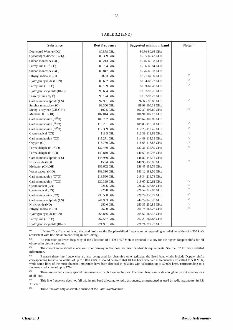
- 38 -
Chapter 3 Radio Astronomy
TABLE 3.2 (END)
Substance Rest frequency Suggested minimum band Notes(1)
Deuterated Water (HDO)
Cyclopropenylidene (C3H2)
80.578 GHz
85.339 GHz
80.50-80.66 GHz
85.05-85.42 GHz
Silicon monoxide (SiO) 86.243 GHz 86.16-86.33 GHz
Formylium (H13CO+) 86.754 GHz 86.66-86.84 GHz
Silicon monoxide (SiO) 86.847 GHz 86.76-86.93 GHz
Ethynyl radical (C2H) 87.3 GHz 87.21-87.39 GHz (5)
Hydrogen cyanide (HCN) 88.632 GHz 88.34-88.72 GHz (4)
Formylium (HCO+) 89.189 GHz 88.89-89.28 GHz (4)
Hydrogen isocyanide (HNC) 90.664 GHz 90.57-90.76 GHz
Diazenylium (N2H+) 93.174 GHz 93.07-93.27 GHz
Carbon monosulphide (CS)
Sulphur monoxide (SO)
Methyl acetylene (CH3C2H)
Methanol (CH3OH)
97.981 GHz
99.300 GHz
102.5 GHz
107.014 GHz
97.65- 98.08 GHz
99.98-100.18 GHz
102.39-102.60 GHz
106.91-107.12 GHz
(4)
(5)
Carbon monoxide (C18O) 109.782 GHz 109.67-109.89 GHz
Carbon monoxide (13CO) 110.201 GHz 109.83-110.31 GHz (4)
Carbon monoxide (C17O)
Cyano radical (CN)
112.359 GHz
113.5 GHz
112.25-112.47 GHz
113.39-113.61 GHz
(6)
(5)
Carbon monoxide (CO)
Oxygen (O2)
115.271 GHz
118.750 GHz
114.88-115.39 GHz
118.63-118.87 GHz
(4)
(7)
Formaldehyde (H213CO) 137.450 GHz 137.31-137.59 GHz (6)
Formaldehyde (H2CO) 140.840 GHz 140.69-140.98 GHz
Carbon monosulphide (CS)
Nitric oxide (NO)
Methanol (CH3OH)
146.969 GHz
150.4 GHz
156.602 GHz
146.82-147.12 GHz
149.95-150.85 GHz
156.45-156.76 GHz
(5)
Water vapour (H2O) 183.310 GHz 183.12-183.50 GHz
Carbon monoxide (C18O) 219.560 GHz 219.34-219.78 GHz
Carbon monoxide (13CO)
Cyano radical (CN)
Cyano radical (CN)
220.399 GHz
226.6 GHz
226.8 GHz
219.67-220.62 GHz
226.37-226.83 GHz
226.57-227.03 GHz
(4)
(5)
(5)
Carbon monoxide (CO) 230.538 GHz 229.77-230.77 GHz (4)
Carbon monosulphide (CS)
Nitric oxide (NO)
Ethynyl radical (C2H)
244.953 GHz
250.6 GHz
262.0 GHz
244.72-245.20 GHz
250.35-250.85 GHz
261.74-262.26 GHz
(6)
(5)
(5)
Hydrogen cyanide (HCN) 265.886 GHz 265.62-266.15 GHz
Formylium (HCO) 267.557 GHz 267.29-267.83 GHz
Hydrogen isocyanide (HNC) 271.981 GHz 271.71-272.25 GHz
(1) If Notes (2) or (4) are not listed, the band limits are the Doppler-shifted frequencies corresponding to radial velocities of 300 km/s (consistent with line radiation occurring in our Galaxy). (2) An extension to lower frequency of the allocation of 1 400-1 427 MHz is required to allow for the higher Doppler shifts for HI
observed in distant galaxies. (3) The current international allocation is not primary and/or does not meet bandwidth requirements. See the RR for more detailed
information. (4) Because these line frequencies are also being used for observing other galaxies, the listed bandwidths include Doppler shifts
corresponding to radial velocities of up to 1 000 km/s. It should be noted that HI has been observed at frequencies redshifted to 500 MHz,
while some lines of the most abundant molecules have been detected in galaxies with velocities up to 50 000 km/s, corresponding to a
frequency reduction of up to 17%. (5) There are several closely spaced lines associated with these molecules. The listed bands are wide enough to permit observations
of all lines. (6) This line frequency does not fall within any band allocated to radio astronomy, or mentioned as used by radio astronomy, in RR
Article 5. (7) These lines are only observable outside of the Earth’s atmosphere.

- 39 -
Radio Astronomy Chapter 3
– 3
9 –
TABLE 3.3
Radio-frequency lines of the greatest importance to radio astronomy
at frequencies between 275 and 1 000 GHz
Substance Rest frequency
(GHz)
Suggested minimum band
(GHz) Notes(1)
Diazenylium (N2H)
Carbon monosulphide (CS)
Hydronium (H3O)
Deuterated water (HDO)
279.511
293.912
307.192
313.750
279.23-279.79
292.93-294.21
306.88-307.50
313.44-314.06
Carbon monoxide (C18O) 329.330 329.00-329.66
Carbon monoxide (13CO) 330.587 330.25-330.92
Carbon monosulphide (CS) 342.883 342.54-343.23
Carbon monoxide (CO) 345.796 345.45-346.14
Hydrogen cyanide (HCN) 354.484 354.13-354.84
Formylium (HCO)
Oxygen (O2)
356.734
368.498
356.37-357.09
368.13-368.87
Diazenylium (N2H) 372.672 372.30-373.05 (2)
Water vapour (H2O)
Hydronium (H3O)
Carbon monosulphide (CS)
Oxygen (O2)
380.197
388.459
391.847
424.763
379.81-380.58
388.07-388.85
390.54-392.24
424.34-425.19
(2)
Carbon monoxide (C18O) 439.088 438.64-439.53
Carbon monoxide (13CO) 440.765 440.32-441.21
Carbon monoxide (CO) 461.041 460.57-461.51
Deuterated water (HDO) 464.925 464.46-465.39
Carbon (CI)
Deuterated water (HDO)
Hydrogen cyanide (HCN)
Carbon monosulphide (CS)
492.162
509.292
531.716
538.689
491.66-492.66
508.78-509.80
529.94-532.25
536.89-539.23
(2) (2)
Water vapour (H218O)
Carbon monoxide (13CO)
547.676
550.926
547.13-548.22
549.09-551.48
(2) (2)
Water vapour (H2O) 556.936 556.37-557.50 (2)
Ammonia (15NH3) 572.113 571.54-572.69 (2)
Ammonia (NH3)
Carbon monoxide (CO)
Carbon monosulphide (CS)
Deuterated water (HDO)
Water vapour (H2O)
Hydrogen chloride (HCl)
Hydrogen chloride (HCl)
Carbon monosulphide (CS)
Carbon monoxide (13CO)
572.498
576.268
587.616
599.927
620.700
625.040
625.980
636.532
661.067
571.92-573.07
574.35-576.84
587.03-588.20
599.33-600.53
620.08-621.32
624.27-625.67
625.35-626.61
634.41-637.17
658.86-661.73
(2) (2) (2) (2) (2)
Carbon monoxide (CO)
Oxygen (O2)
Carbon monosulphide (CS)
Water vapour (H2O)
Oxygen (O2)
691.473
715.393
734.324
752.033
773.840
690.78-692.17
714.68-716.11
733.59-735.06
751.28-752.79
773.07-884.61
(2) (2) (2) (2)
Hydrogen cyanide (HCN) 797.433 796.64-798.23
Formylium (HCO) 802.653 801.85-803.85
Carbon monoxide (CO) 806.652 805.85-807.46
Carbon (CI) 809.350 808.54-810.16
Carbon monosulphide (CS) 832.057 829.28-832.89
Oxygen (O2) 834.146 833.31-834.98
Carbon monosulphide (CS) 880.899 877.96-881.78
Water vapour (H2O) 916.172 915.26-917.09 (2)
Carbon monoxide (CO) 921.800 918.72-922.72 (2)
Carbon monosulphide (CS) 929.723 926.62-930.65
Water vapour (H2O) 970.315 969.34-971.29 (2)
Carbon monosulphide (CS) 978.529 977.55-979.51 (2)
Water vapour (H2O) 987.927 986.94-988.92 (2)
(1) The band limits are the Doppler-shifted frequencies corresponding to radial velocities of 300 km/s (consistent with line radiation occurring in our Galaxy).
(2) These lines are only observable outside of the Earth’s atmosphere.
- 40 -
Chapter 4 Radio Astronomy
CHAPTER 4
Vulnerability of radio astronomy observations to interference
4.1 Introduction
The radiation measured in radio astronomy has, in almost all cases, a Gaussian probability distribution in
amplitude. Except in the case of narrow-band spectral line emissions, it has the same statistical
characteristics as thermal noise radiation from the Earth, its atmosphere, or noise generated in a receiver
itself. Moreover, the cosmic radio emissions are very weak. In radio astronomy observations, the S/N in the
RF and IF parts of the receiver is typically in the range -20 dB to –60 dB, i.e. the power contributed by the
source under study is a factor of 10–2
to 10–6
lower than the unwanted noise power from the atmosphere, the
ground, and the receiver circuits. In most communication systems the corresponding S/N is of the order of
unity or greater. Because radio astronomy signals are so weak in comparison to those of other services, radio
astronomy observations are highly vulnerable to radio interference and, except in the case of pulsars, cosmic
signals generally have no characteristic modulation that would help to distinguish them from noise or from
many forms of interfering signals.
The reason observations with very low S/N can give useful measurements is that whereas in other radio
services the information is usually in changes in the properties of the transmission (i.e. the modulation), radio
astronomical measurements are usually of the average properties of the signal. When the total noise power in
the receiver IF stages is measured using a detector, and the output of the detector is averaged for many
seconds, or in some cases many hours, the statistical fluctuations in the measured values are greatly reduced.
It is now possible to detect fractional changes in the total noise level that are of the order of 10–8
of the
average level, and this requires the averaging of at least 1016
independent samples. An example of the high
sensitivity of radio astronomy observations is the mapping of the angular structure in the cosmic background
radiation by the PLANCK satellite (Planck Collaboration et al 2011) that is currently operating at the L2
Sun-Earth Lagrange Point noted in Recommendation ITU-R RA.1417. Fluctuations of the order of 10–6
of
the 2.8 K background temperature have been measured, 75 dB or more below the system noise temperatures
of the receivers on the satellite. The high sensitivity of such observations is obtained at the expense of
information on short-time variations of any signal characteristics, which are lost in the averaging that is
essential in reducing the noise fluctuations. The discovery of these fluctuations [Smoot et al 1992], which
signal the origin of the large-scale structure in the present-day Universe, was the subject of the 2006 Nobel
Prize in Physics, the fourth such Prize to be awarded for radio astronomical investigations.
As a historical note, the method of analysis of threshold levels of interference in this Chapter originated in
the Annex of ex-CCIR Report 224-1 [Oslo, 1966]. The interference threshold levels in that Report, with
subsequent revisions and additions, provide a basis for frequency coordination in radio astronomy and are
included in Annex 1 of Recommendation ITU-R RA.769, and Tables 4.1 and 4.2 in this Chapter.
4.2 Basic considerations in the calculation of interference levels
4.2.1 Detrimental-level criterion for interference
In practice, the increased power level at the receiver output resulting from the presence of an interfering
signal is not sufficiently constant that it can be calibrated and subtracted from the measured power. In
addition to the changes intrinsic to the modulation of the transmissions, interfering signals that have
propagated over long distances show large amplitude fluctuations resulting from variations in the atmosphere
and in other factors that influence the path loss. Signals from mobile stations on vehicles that are moving
vary as the path between the transmitter and the radio telescope changes. Even if the interfering pfd is
constant, the received power level varies as the source-tracking motion of the radio telescope presents
varying side-lobe levels in the direction of the transmitter. At low levels, interference has the effect of adding
fluctuations which may not generally be distinguishable from the fluctuations resulting from the system
noise, or in some cases from the astronomical signal. However, in general, the receiver output fluctuations
due to interference do not average out with increasing the integration time in the same manner as purely
random noise.

- 41 -
Radio Astronomy Chapter 4
– 4
1 –
The criterion used to define the intensity at which an interfering signal is considered detrimental (harmful), is
the level of unwanted emissions that causes an increase of 10% in the measurement errors, relative to the
errors due to the system noise alone. In interference calculations the usual practice is to assume that this
interference level is the same as that which causes an increase in the receiver output by 10% of the root mean
square (r.m.s.) output fluctuations due to the system noise. Consider a typical measurement in which the
power received from a radio source is measured by taking the difference of the receiver output first with the
antenna pointed at the source, and then with it offset in position, in order to measure the sky background
level. Suppose that the interference is present during the measurement on the radio source but not present
during the reference measurement of the background level, or vice versa, as might occur in the case of an
intermittent communication signal. Then if the interference at the receiver output is 10% of the r.m.s. noise
level, the total error in the measurement of the power from the source is increased by as much as 10%. One
can visualize this effect as increasing by 10% the length of the error bars on measurements of the strength of
a radio source, which might be plotted as a function of some other astronomical parameter. Note also that, in
the absence of interference, a 10% increase in the r.m.s. uncertainty of the measurement is equivalent to a
loss of 20% in observing time. Under these conditions useful measurements are still possible, but the data are
significantly degraded.
4.2.2 Antenna response pattern
Radio astronomy observations are usually made using large, high-gain antennas or antenna arrays, in order to
provide the required sensitivity and angular resolution on the sky. Radio telescopes may consist of large,
single antennas, or arrays of many antennas. With a typical beamwidth ranging from a few seconds of arc to
a few degrees, the probability of a source of interference falling within the main beam is generally small
enough that we need only consider interference entering through the side-lobes. A recommended model for
the side-lobes of large parabolic antennas is given in Recommendation ITU-R SA.509 – Space applications
and meteorology series, which is based on empirical data from a number of large antennas. It applies to
antennas of diameter greater than 100 wavelengths, for frequencies between 2 GHz and 30 GHz, and for
values of angle , measured from the axis of the main beam, greater than 1. The side-lobe gain varies on an
angular scale of order /D, where is the wavelength and D the width of the antenna aperture. The model for
the envelope of the gain (G) of the side-lobes is then given by:
The effect of an interfering signal clearly depends upon the angle of incidence relative to the main beam axis
(the boresight) of the antenna since the side-lobe gain, as represented by the model, varies from 32 to –10
dB as a function of this angle. However, in § 4.3 it is useful to calculate threshold levels of detrimental
interference for a particular side-lobe level, and for this we use 0 dBi. For the side-lobe model in equation
(4.1), a value of 0 dBi, i.e. a gain equal to that of an isotropic radiator, occurs at 19.1 from the main beam.
Note that if we compute the threshold level of pfd or spfd based on reception with side-lobe gain of 0 dBi,
then the threshold of interference in the radio astronomy receiver will be exceeded if the interference is
received through side-lobes with gain greater than 0 dBi, that is, for values of less than 19.1. Thus if a
threshold-level signal is incident in a direction that lies within a cone of half-angle equal to 19.1 centered on
the axis of the main beam, the power received will exceed the detrimental interference criterion. The solid
angle of this cone in radians, , is equal to 2(1 – cos ). A rough measure of the probability of interference
being received within the 19.1 cone is equal to divided by the 2B steradians above the horizon from which
interfering signals may be received. For 19.1, /2B 5.5%. For more recent antenna designs a side-lobe
model of, 29 – 25 log , has been proposed (see, e.g. Recommendation ITU-R S.580). With this model the 0
dBi value of is 14.5, and the corresponding value of /2B is 3.2%. Yet another side-lobe model (see
Recommendation ITU-R S.1428) uses 34 30 log , for which the 0 dBi angle is 13.6 and the
corresponding value of /2B is 2.8%. An upper limit on the aggregate percentage of time that interference
above the detrimental threshold can be tolerated is specified in Recommendation ITU-R RA.1513 as 5%, of
which no more than 2% may come from any one network (see § 4.2.4.). The three values of /2B discussed
above (5.5%, 3.2%, and 2.8%) are in reasonable accord with these figures, and thus lend support to the
G 32 – 25 log dBi for 1 47.8
G = –10 dBi for 47.8 180

- 42 -
Chapter 4 Radio Astronomy
choice of the 0 dBi side-lobe level as appropriate for calculation of the pfd and spfd corresponding to the
detrimental threshold.
The particular case of non-GSO satellites presents a dynamical situation, that is, the positions of the satellites
relative to the beam of the radio astronomy antenna show large changes within the time scale of the 2 000 s
integration time. Analysis of interference in this case requires integrating the response over the varying side-
lobe levels, for example, using the concept of equivalent power flux-density (epfd) defined in RR No. 22.5C.
In addition it is usually necessary to combine the contributions to the radio telescope of a number of satellites
within a particular system. In such calculations it is suggested that, until a model specifically formulated for
radio astronomy antennas becomes available, the antenna response pattern for antennas of diameter greater
than 100 in Recommendation ITU-R S.1428 (see Annex 1 to this Chapter) be used to represent the radio
astronomy antenna.
The side-lobe models described above apply to symmetrical paraboloids that suffer from scattering of
radiation by the focal support structure. Side-lobe levels for offset-feed reflectors with unblocked apertures
are typically 10 to 15 dB lower than those given by the model. Only a few antennas of offset-feed design
have been developed for radio astronomy. For large antennas, symmetrical designs are more economical and
also may be preferred for polarisation measurements.
4.2.3 Averaging time (integration time)
The time averaging process that reduces the noise fluctuations is usually performed in two or more steps.
Data are typically averaged for a few tens of milliseconds to a few tens of seconds and then recorded
digitally. This first step reduces the amount of data, but allows features like short bursts of strong
interference to be removed later without serious loss of data. Further averaging is often done off-line during
subsequent data reduction. For example, an observation might consist of repeated measurements at two or
more different locations in the sky, to compare the power level received from a radio source (plus the sky
background emission) with that from a background reference position. Separate averages would be required
for each position. Data taken at different observing sessions might be included, and the total averaging time
might extend to tens or hundreds of hours [Owen and Morrison, 2009; Walter et al., 2012]. Often the limit is
set by the time available on a large radio telescope. Such long averaging is required when searching for
exceptionally weak signals, where it is quite normal practice to average many individual records of the
spectrum from one point in the sky. In studies of interference thresholds it has been the usual practice to use
2 000 s as a representative averaging time. Longer integration times are also routinely used and 360 000 s
(100 h) could be taken as representative of ground-based observations where exceptionally high sensitivity is
required. Since the sensitivity of an observation varies as the square root of the averaging time, the difference
between 2 000 s and 360 000 s corresponds to a difference of 11.3 dB in the sensitivity to both astronomical
signals and interference. There are also certain observations of time varying phenomena, e.g. observations of
stellar or solar bursts, and interplanetary scintillations for which much shorter time periods may be
appropriate.
4.2.4 Percentage of time lost to interference
In many cases interference is sporadic in nature, for example from mobile communications signals, or shows
large variations in strength with time as a result of propagation conditions. In determining whether such
signals are detrimental to radio astronomy observations it is necessary to specify a maximum percentage of
time for which detrimental interference can be tolerated. For most services, such time percentages can be
found in various recommendations, and usually vary from 0.01% for communications in which safety of life
is involved, to several percent for services involving data collection that can be repeated. In the case of radio
astronomy, a net loss of 5% from all sources is the maximum tolerable figure. Since, for many observations
in radio astronomy, interference from several sources in nearby frequency bands may be encountered, the
maximum tolerable time loss from any one service is 2%. These figures are specified in Recommendation
ITU-R RA.1513. They are essential in making Monte Carlo calculations to determine how to limit sporadic
sources of interference (see § 4.8).
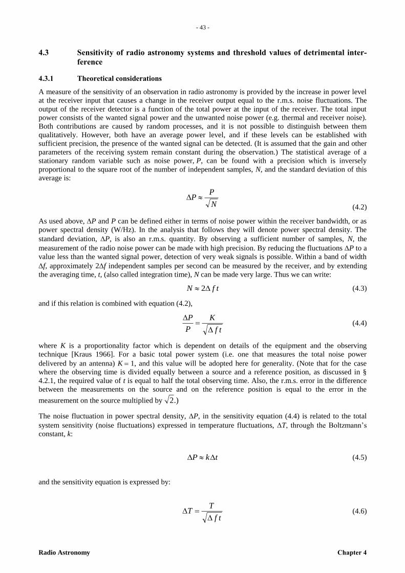
- 43 -
Radio Astronomy Chapter 4
– 4
3 –
4.3 Sensitivity of radio astronomy systems and threshold values of detrimental inter-
ference
4.3.1 Theoretical considerations
A measure of the sensitivity of an observation in radio astronomy is provided by the increase in power level
at the receiver input that causes a change in the receiver output equal to the r.m.s. noise fluctuations. The
output of the receiver detector is a function of the total power at the input of the receiver. The total input
power consists of the wanted signal power and the unwanted noise power (e.g. thermal and receiver noise).
Both contributions are caused by random processes, and it is not possible to distinguish between them
qualitatively. However, both have an average power level, and if these levels can be established with
sufficient precision, the presence of the wanted signal can be detected. (It is assumed that the gain and other
parameters of the receiving system remain constant during the observation.) The statistical average of a
stationary random variable such as noise power, P, can be found with a precision which is inversely
proportional to the square root of the number of independent samples, N, and the standard deviation of this
average is:
N
PP
(4.2)
As used above, P and P can be defined either in terms of noise power within the receiver bandwidth, or as
power spectral density (W/Hz). In the analysis that follows they will denote power spectral density. The
standard deviation, P, is also an r.m.s. quantity. By observing a sufficient number of samples, N, the
measurement of the radio noise power can be made with high precision. By reducing the fluctuations P to a
value less than the wanted signal power, detection of very weak signals is possible. Within a band of width
f, approximately 2f independent samples per second can be measured by the receiver, and by extending
the averaging time, t, (also called integration time), N can be made very large. Thus we can write:
tfN 2 (4.3)
and if this relation is combined with equation (4.2),
tf
K
P
P
(4.4)
where K is a proportionality factor which is dependent on details of the equipment and the observing
technique [Kraus 1966]. For a basic total power system (i.e. one that measures the total noise power
delivered by an antenna) K 1, and this value will be adopted here for generality. (Note that for the case
where the observing time is divided equally between a source and a reference position, as discussed in §
4.2.1, the required value of t is equal to half the total observing time. Also, the r.m.s. error in the difference
between the measurements on the source and on the reference position is equal to the error in the
measurement on the source multiplied by .)2
The noise fluctuation in power spectral density, P, in the sensitivity equation (4.4) is related to the total
system sensitivity (noise fluctuations) expressed in temperature fluctuations, T, through the Boltzmann’s
constant, k:
tkP (4.5)
and the sensitivity equation is expressed by:
tf
TT
(4.6)
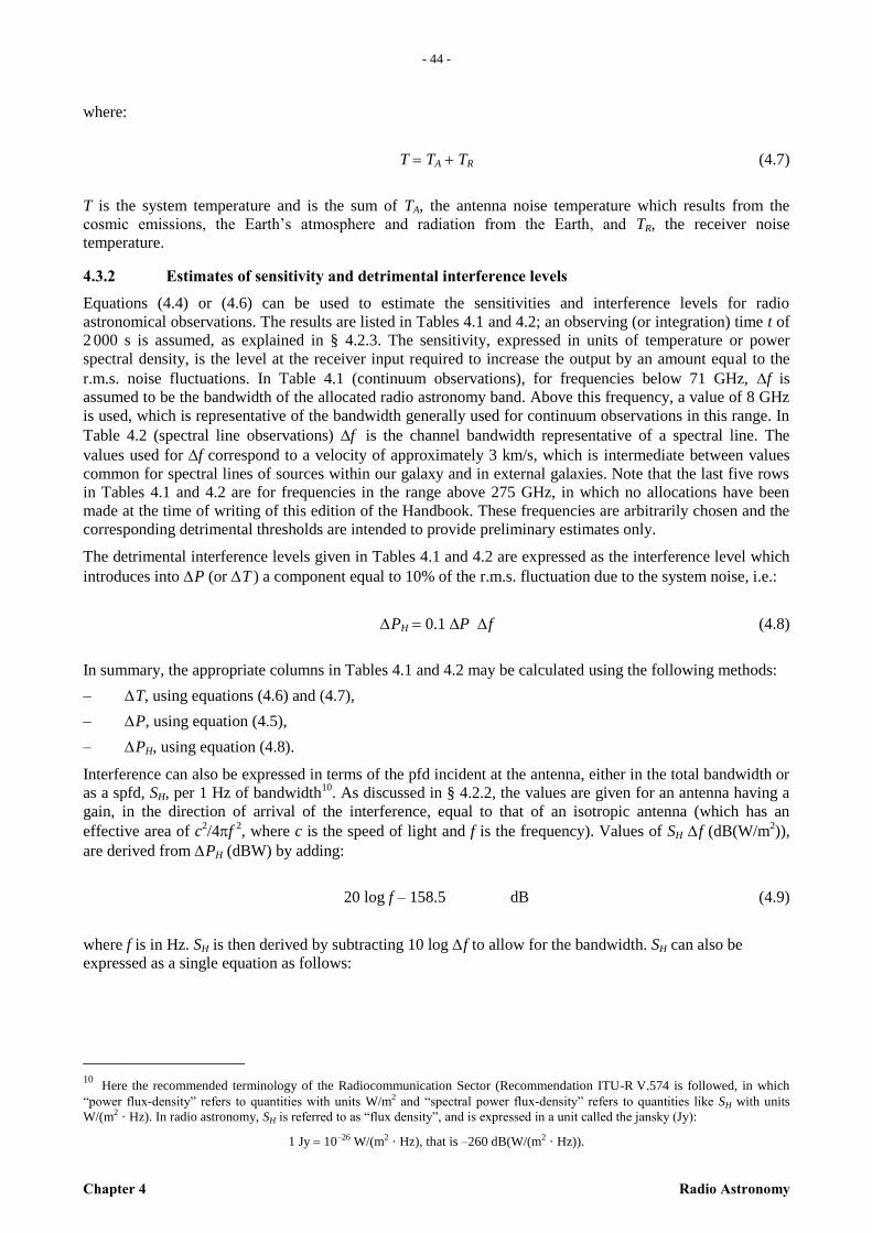
- 44 -
Chapter 4 Radio Astronomy
where:
T TA TR (4.7)
T is the system temperature and is the sum of TA, the antenna noise temperature which results from the
cosmic emissions, the Earth’s atmosphere and radiation from the Earth, and TR, the receiver noise
temperature.
4.3.2 Estimates of sensitivity and detrimental interference levels
Equations (4.4) or (4.6) can be used to estimate the sensitivities and interference levels for radio
astronomical observations. The results are listed in Tables 4.1 and 4.2; an observing (or integration) time t of
2 000 s is assumed, as explained in § 4.2.3. The sensitivity, expressed in units of temperature or power
spectral density, is the level at the receiver input required to increase the output by an amount equal to the
r.m.s. noise fluctuations. In Table 4.1 (continuum observations), for frequencies below 71 GHz, f is
assumed to be the bandwidth of the allocated radio astronomy band. Above this frequency, a value of 8 GHz
is used, which is representative of the bandwidth generally used for continuum observations in this range. In
Table 4.2 (spectral line observations) f is the channel bandwidth representative of a spectral line. The
values used for f correspond to a velocity of approximately 3 km/s, which is intermediate between values
common for spectral lines of sources within our galaxy and in external galaxies. Note that the last five rows
in Tables 4.1 and 4.2 are for frequencies in the range above 275 GHz, in which no allocations have been
made at the time of writing of this edition of the Handbook. These frequencies are arbitrarily chosen and the
corresponding detrimental thresholds are intended to provide preliminary estimates only.
The detrimental interference levels given in Tables 4.1 and 4.2 are expressed as the interference level which
introduces into P (or T ) a component equal to 10% of the r.m.s. fluctuation due to the system noise, i.e.:
PH 0.1 P f (4.8)
In summary, the appropriate columns in Tables 4.1 and 4.2 may be calculated using the following methods:
– T, using equations (4.6) and (4.7),
– P, using equation (4.5),
– PH, using equation (4.8).
Interference can also be expressed in terms of the pfd incident at the antenna, either in the total bandwidth or
as a spfd, SH, per 1 Hz of bandwidth10
. As discussed in § 4.2.2, the values are given for an antenna having a
gain, in the direction of arrival of the interference, equal to that of an isotropic antenna (which has an
effective area of c2/4f
2, where c is the speed of light and f is the frequency). Values of SH f (dB(W/m
2)),
are derived from PH (dBW) by adding:
20 log f – 158.5 dB (4.9)
where f is in Hz. SH is then derived by subtracting 10 log f to allow for the bandwidth. SH can also be
expressed as a single equation as follows:
____________________
10 Here the recommended terminology of the Radiocommunication Sector (Recommendation ITU-R V.574 is followed, in which
“power flux-density” refers to quantities with units W/m2 and “spectral power flux-density” refers to quantities like SH with units
W/(m2 · Hz). In radio astronomy, SH is referred to as “flux density”, and is expressed in a unit called the jansky (Jy):
1 Jy 10–26 W/(m2 · Hz), that is –260 dB(W/(m2 · Hz)).
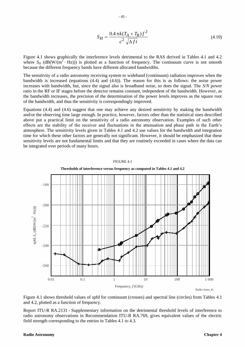
- 45 -
Radio Astronomy Chapter 4
– 4
5 –
tfc
fTTkS RA
H
2
2)(4.0 (4.10)
Figure 4.1 shows graphically the interference levels detrimental to the RAS derived in Tables 4.1 and 4.2
where SH (dB(W/(m2 · Hz))) is plotted as a function of frequency. The continuum curve is not smooth
because the different frequency bands have different allocated bandwidths.
The sensitivity of a radio astronomy receiving system to wideband (continuum) radiation improves when the
bandwidth is increased (equations (4.4) and (4.6)). The reason for this is as follows: the noise power
increases with bandwidth, but, since the signal also is broadband noise, so does the signal. The S/N power
ratio in the RF or IF stages before the detector remains constant, independent of the bandwidth. However, as
the bandwidth increases, the precision of the determination of the power levels improves as the square root
of the bandwidth, and thus the sensitivity is correspondingly improved.
Equations (4.4) and (4.6) suggest that one may achieve any desired sensitivity by making the bandwidth
and/or the observing time large enough. In practice, however, factors other than the statistical ones described
above put a practical limit on the sensitivity of a radio astronomy observation. Examples of such other
effects are the stability of the receiver and fluctuations in the attenuation and phase path in the Earth’s
atmosphere. The sensitivity levels given in Tables 4.1 and 4.2 use values for the bandwidth and integration
time for which these other factors are generally not significant. However, it should be emphasized that these
sensitivity levels are not fundamental limits and that they are routinely exceeded in cases where the data can
be integrated over periods of many hours.
FIGURE 4.1
Thresholds of interference versus frequency as computed in Tables 4.1 and 4.2
Radio-Astro_41Frequency, (GHz)f
spfd
, (
dB
(W/(
m ·
Hz)
))S
H
2
0.01 0.1 1 10 100 1 000
–260
–200
–240
–180
–220
Figure 4.1 shows threshold values of spfd for continuum (crosses) and spectral line (circles) from Tables 4.1
and 4.2, plotted as a function of frequency.
Report ITU-R RA.2131 - Supplementary information on the detrimental threshold levels of interference to
radio astronomy observations in Recommendation ITU-R RA.769, gives equivalent values of the electric
field strength corresponding to the entries in Tables 4.1 to 4.3.
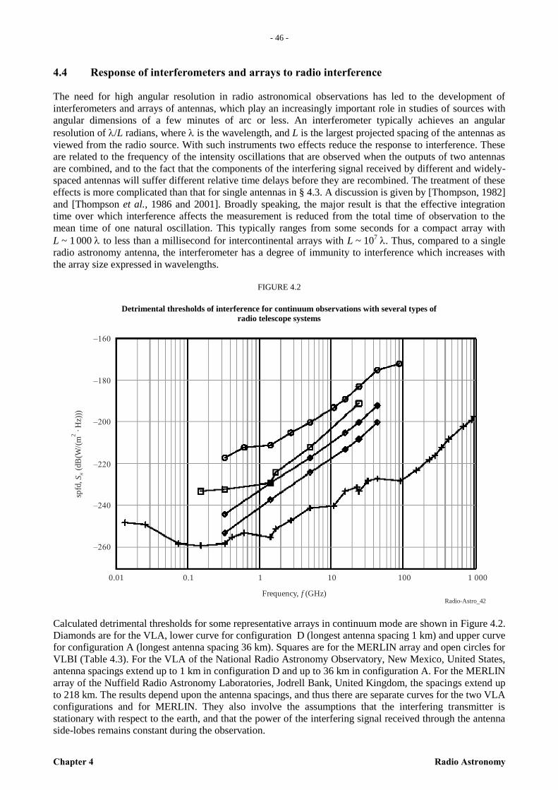
- 46 -
Chapter 4 Radio Astronomy
4.4 Response of interferometers and arrays to radio interference
The need for high angular resolution in radio astronomical observations has led to the development of
interferometers and arrays of antennas, which play an increasingly important role in studies of sources with
angular dimensions of a few minutes of arc or less. An interferometer typically achieves an angular
resolution of /L radians, where is the wavelength, and L is the largest projected spacing of the antennas as
viewed from the radio source. With such instruments two effects reduce the response to interference. These
are related to the frequency of the intensity oscillations that are observed when the outputs of two antennas
are combined, and to the fact that the components of the interfering signal received by different and widely-
spaced antennas will suffer different relative time delays before they are recombined. The treatment of these
effects is more complicated than that for single antennas in § 4.3. A discussion is given by [Thompson, 1982]
and [Thompson et al., 1986 and 2001]. Broadly speaking, the major result is that the effective integration
time over which interference affects the measurement is reduced from the total time of observation to the
mean time of one natural oscillation. This typically ranges from some seconds for a compact array with
L ~ 1 000 to less than a millisecond for intercontinental arrays with L ~ 107 . Thus, compared to a single
radio astronomy antenna, the interferometer has a degree of immunity to interference which increases with
the array size expressed in wavelengths.
FIGURE 4.2
Detrimental thresholds of interference for continuum observations with several types of
radio telescope systems
Radio-Astro_42Frequency, (GHz)f
spfd
, (
dB
(W/(
m ·
Hz)
))S
H
2
0.01 0.1 1 10 100 1 000
–260
–200
–240
–180
–160
–220
Calculated detrimental thresholds for some representative arrays in continuum mode are shown in Figure 4.2.
Diamonds are for the VLA, lower curve for configuration D (longest antenna spacing 1 km) and upper curve
for configuration A (longest antenna spacing 36 km). Squares are for the MERLIN array and open circles for
VLBI (Table 4.3). For the VLA of the National Radio Astronomy Observatory, New Mexico, United States,
antenna spacings extend up to 1 km in configuration D and up to 36 km in configuration A. For the MERLIN
array of the Nuffield Radio Astronomy Laboratories, Jodrell Bank, United Kingdom, the spacings extend up
to 218 km. The results depend upon the antenna spacings, and thus there are separate curves for the two VLA
configurations and for MERLIN. They also involve the assumptions that the interfering transmitter is
stationary with respect to the earth, and that the power of the interfering signal received through the antenna
side-lobes remains constant during the observation.
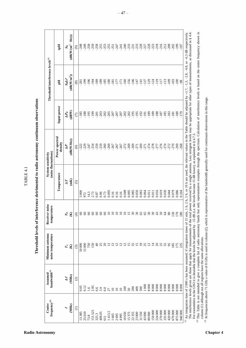
Radio Astronomy Chapter 4
– 47 –
TA
BL
E 4
.1
Th
resh
old
lev
els
of
inte
rfer
ence
det
rim
enta
l to
ra
dio
ast
ron
om
y c
on
tin
uu
m o
bse
rv
ati
on
s
Cen
tre
freq
uen
cy(2
)
f
(MH
z)
Ass
um
ed
ba
nd
wid
th(3
)
f
(MH
z)
Min
imu
m a
nte
nn
a
no
ise t
em
pera
ture
T
A
(K)
Recei
ver n
ois
e
tem
pera
ture
T
R
(K)
Sy
stem
sen
siti
vit
y
(no
ise
flu
ctu
ati
on
s)
Th
resh
old
in
terfe
ren
ce
levels
(1)
Tem
pera
ture
Pow
er s
pec
tra
l d
en
sity
In
pu
t p
ow
er
pfd
sp
fd
T
(mK
)
P
(dB
(W/H
z))
P
H
(dB
W)
SH
f
(dB
(W/m
2))
SH
(dB
(W/(
m2 ·
Hz)
))
(1)
(2)
(3)
(4)
(5)
(6)
(7)
(8)
(9)
13.3
85
25.6
10
73.8
151
.52
5
325
.3
408
.05
611
1 4
13
.5
1 6
65
2 6
95
4 9
95
10
650
15
375
22
355
23
800
31
550
43
000
89
000
150
00
0
224
00
0
270
00
0
335
00
0
420
00
0
670
00
0
875
00
0
940
00
0
0.0
5
0.1
2
1.6
2.9
5
6.6
3.9
6.0
27
10
10
10
100
50
290
400
500
1 0
00
8 0
00
8 0
00
8 0
00
8 0
00
8 0
00
8 0
00
8 0
00
8 0
00
8 0
00
50
000
15
000
750
150
40
25
20
12
12
12
12
12
15
35
15
18
25
12
14
20
25
55
95
185
175
235
60
60
60
60
60
60
60
10
10
10
10
10
15
30
30
65
65
30
30
43
50
64
80
130
170
180
5 0
00
972
14.3
2.7
3
0.8
7
0.9
6
0.7
3
0.0
95
0.1
6
0.1
6
0.1
6
0.0
49
0.0
95
0.0
85
0.0
50
0.0
83
0.0
64
0.0
11
0.0
11
0.0
16
0.0
19
0.0
30
0.0
44
0.0
79
0.0
86
0.1
04
–222
–229
–247
–254
–259
–259
–260
–269
–267
–267
–267
–272
–269
–269
–271
–269
–271
–274
–278
–277
–276
–274
–272
–270
–269
–268
–185
–188
–195
–199
–201
–203
–202
–205
–207
–207
–207
–202
–202
–195
–195
–192
–191
–189
–189
–188
–187
–185
–183
–181
–180
–179
–201
–199
–196
–194
–189
–189
–185
–180
–181
–177
–171
–160
–156
–146
–147
–141
–137
–129
–124
–119
–117
–113
–109
–103
–100
–98
–248
–249
–258
–259
–258
–255
–253
–255
–251
–247
–241
–240
–233
–231
–233
–228
–227
–228
–223
–218
–216
–212
–208
–202
–199
–197
(1) A
n i
nte
gra
tion
tim
e of
2 0
00
s h
as b
een
ass
um
ed;
if i
nte
gra
tion
tim
es o
f 15
min
, 1
h,
2 h
, 5
h,
or
10
h a
re u
sed
, th
e re
levan
t val
ues
in
th
e T
able
sh
ould
be
adju
sted
by
1.7
, –1
.3,
–2
.8,
–4.8
, or
–6.3
dB
res
pec
tivel
y.
Th
e in
terf
eren
ce l
evel
s giv
en a
re t
hose
th
at a
pp
ly f
or
mea
sure
men
ts o
f th
e to
tal
pow
er r
ece
ived
by a
sin
gle
an
ten
na.
Les
s st
rin
gen
t le
vel
s m
ay b
e ap
pro
pri
ate
for
oth
er t
yp
es o
f m
easu
rem
ents
, as
dis
cuss
ed i
n §
4.4
.
Fo
r tr
ansm
itte
rs i
n t
he
GS
O i
t is
des
irab
le t
hat
th
e le
vel
s b
e ad
just
ed b
y –
15 d
B (
i.e.
th
e le
vel
s b
ecom
e 1
5 d
B l
ow
er),
as
exp
lain
ed i
n §
4.7
.3.
(2) T
his
Tab
le i
s n
ot
inte
nd
ed t
o g
ive
a co
mp
lete
lis
t of
rad
io a
stro
nom
y b
and
s bu
t on
ly r
epre
sen
tati
ve
exam
ple
s th
rou
gh
th
e sp
ectr
um
. C
alcu
lati
on o
f in
terf
eren
ce l
evel
s is
bas
ed o
n t
he
cen
tre
freq
uen
cy s
how
n i
n
colu
mn
(1
) al
thou
gh
not
all
regio
ns
hav
e th
e sa
me
allo
cati
on
s.
(3) A
t fr
equ
enci
es a
bove
71 G
Hz
a val
ue
of
8 G
Hz
is u
sed
in c
olu
mn
(2
), w
hic
h i
s re
pre
sen
tati
ve
of
the
ban
dw
idth
gen
eral
ly u
sed
for
con
tin
uu
m o
bse
rvat
ion
s in
this
ran
ge.
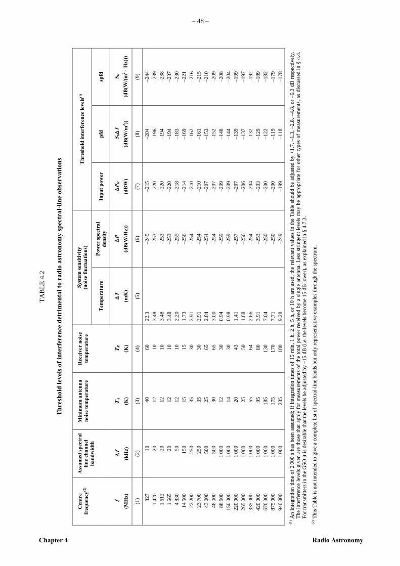
Chapter 4 Radio Astronomy
– 48 –
TA
BL
E 4
.2
Th
resh
old
lev
els
of
inte
rfer
ence
det
rim
enta
l to
ra
dio
ast
ron
om
y s
pec
tra
l-li
ne
ob
serv
ati
on
s
Cen
tre
freq
uen
cy(2
)
f
(MH
z)
Ass
um
ed
sp
ectr
al
lin
e ch
an
nel
ba
nd
wid
th
f
(kH
z)
Min
imu
m a
nte
nn
a
no
ise t
em
pera
ture
TA
(K)
Recei
ver n
ois
e
tem
pera
ture
TR
(K)
Sy
stem
sen
siti
vit
y
(no
ise
flu
ctu
ati
on
s)
Th
resh
old
in
terfe
ren
ce
levels
(1)
Tem
pera
ture
Pow
er s
pec
tra
l
den
sity
In
pu
t p
ow
er
pfd
sp
fd
T
(mK
)
P
(dB
(W/H
z))
P
H
(dB
W)
SH
f
(dB
(W/m
2))
SH
(dB
(W/(
m2 ·
Hz)
))
(1)
(2)
(3)
(4)
(5)
(6)
(7)
(8)
(9)
327
1 4
20
1 6
12
1 6
65
4 8
30
14
500
22
200
23
700
43
000
48
000
88
600
150
00
0
220
00
0
265
00
0
335
00
0
420
00
0
670
00
0
875
00
0
940
00
0
10
20
20
20
50
150
250
250
500
500
1 0
00
1 0
00
1 0
00
1 0
00
1 0
00
1 0
00
1 0
00
1 0
00
1 0
00
40
12
12
12
12
15
35
35
25
30
12
14
20
25
55
95
185
175
235
60
10
10
10
10
15
30
30
65
65
30
30
43
50
64
80
130
170
180
22.3
3.4
8
3.4
8
3.4
8
2.2
0
1.7
3
2.9
1
2.9
1
2.8
4
3.0
0
0.9
4
0.9
8
1.4
1
1.6
8
2.6
6
3.9
1
7.0
4
7.7
1
9.2
8
–245
–253
–253
–253
–255
–256
–254
–254
–254
–254
–259
–259
–257
–256
–254
–253
–250
–250
–249
–215
–220
–220
–220
–218
–214
–210
–210
–207
–207
–209
–209
–207
–206
–204
–203
–200
–200
–199
–204
–196
–194
–194
–183
–169
–162
–161
–153
–152
–148
–144
–139
–137
–132
–129
–122
–119
–118
–244
–239
–238
–237
–230
–221
–216
–215
–210
–209
–208
–204
–199
–197
–192
–189
–182
–179
–178
(1) A
n i
nte
gra
tion
tim
e of
2 0
00 s
has
bee
n a
ssum
ed;
if i
nte
gra
tion
tim
es o
f 15
min
, 1
h,
2 h
, 5
h,
or
10 h
are
use
d,
the r
elev
ant
val
ues
in
th
e T
able
sh
ould
be
adju
sted
by +
1.7
, –1
.3,
–2
.8,
–4.8
, or
–6.3
dB
res
pec
tivel
y.
Th
e in
terf
eren
ce l
evel
s giv
en a
re t
hose
th
at a
pp
ly f
or
mea
sure
men
ts o
f th
e to
tal
pow
er r
ecei
ved
by a
sin
gle
an
ten
na.
Les
s st
rin
ge
nt
level
s m
ay b
e ap
pro
pri
ate
for
oth
er t
yp
es o
f m
easu
rem
ents
, as
dis
cuss
ed i
n §
4.4
. F
or
tran
smit
ters
in t
he
GS
O i
t is
des
irab
le t
hat
th
e le
vel
s b
e ad
just
ed b
y –
15 d
B (
i.e.
th
e le
vel
s b
ecom
e 1
5 d
B l
ow
er),
as
exp
lain
ed i
n §
4.7
.3.
(2) T
his
Tab
le i
s n
ot
inte
nd
ed t
o g
ive
a co
mp
lete
lis
t of
spec
tral
-lin
e b
and
s b
ut
on
ly r
epre
sen
tati
ve
exam
ple
s th
rou
gh
th
e sp
ectr
um
.
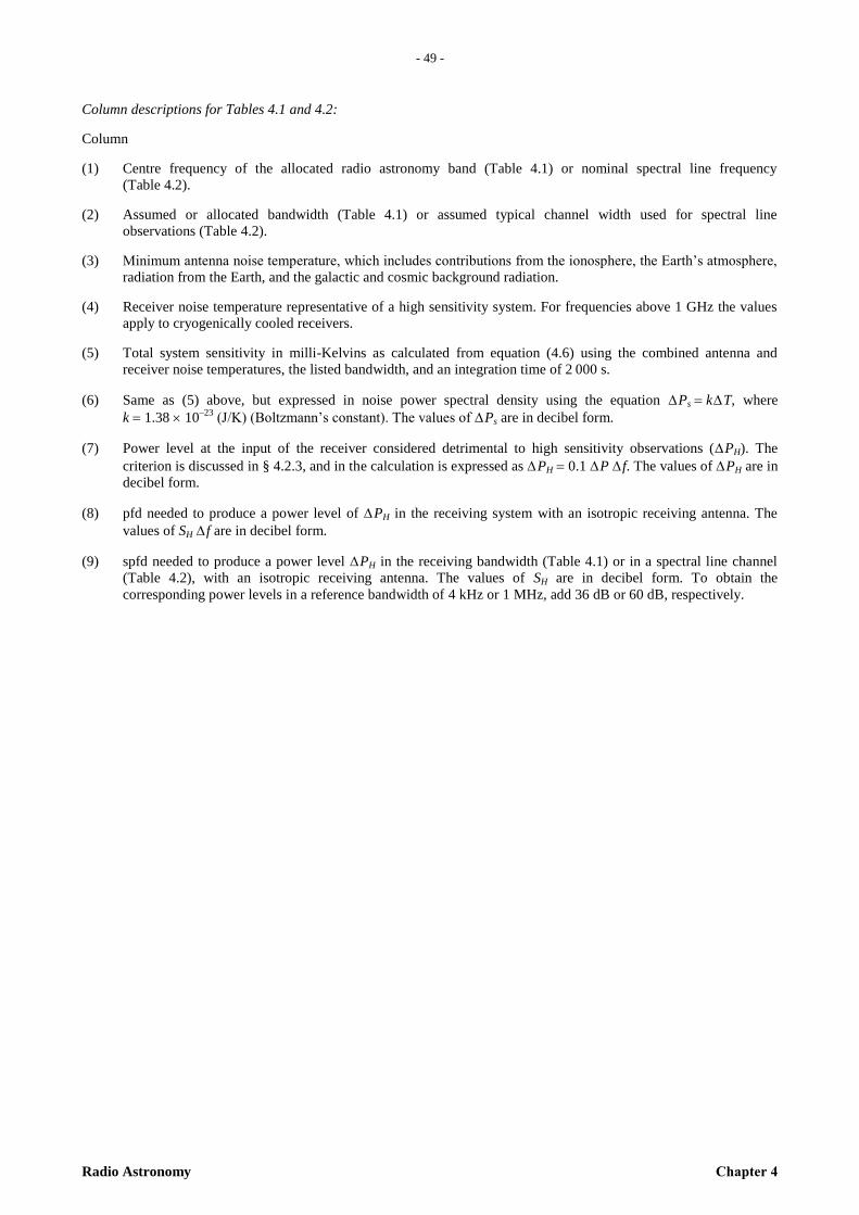
- 49 -
Radio Astronomy Chapter 4
– 4
9 –
Column descriptions for Tables 4.1 and 4.2:
Column
(1) Centre frequency of the allocated radio astronomy band (Table 4.1) or nominal spectral line frequency
(Table 4.2).
(2) Assumed or allocated bandwidth (Table 4.1) or assumed typical channel width used for spectral line
observations (Table 4.2).
(3) Minimum antenna noise temperature, which includes contributions from the ionosphere, the Earth’s atmosphere,
radiation from the Earth, and the galactic and cosmic background radiation.
(4) Receiver noise temperature representative of a high sensitivity system. For frequencies above 1 GHz the values
apply to cryogenically cooled receivers.
(5) Total system sensitivity in milli-Kelvins as calculated from equation (4.6) using the combined antenna and
receiver noise temperatures, the listed bandwidth, and an integration time of 2 000 s.
(6) Same as (5) above, but expressed in noise power spectral density using the equation Ps k T, where
k 1.38 10–23
(J/K) (Boltzmann’s constant). The values of Ps are in decibel form.
(7) Power level at the input of the receiver considered detrimental to high sensitivity observations ( PH). The
criterion is discussed in § 4.2.3, and in the calculation is expressed as PH 0.1 P f. The values of PH are in
decibel form.
(8) pfd needed to produce a power level of PH in the receiving system with an isotropic receiving antenna. The
values of SH f are in decibel form.
(9) spfd needed to produce a power level PH in the receiving bandwidth (Table 4.1) or in a spectral line channel
(Table 4.2), with an isotropic receiving antenna. The values of SH are in decibel form. To obtain the
corresponding power levels in a reference bandwidth of 4 kHz or 1 MHz, add 36 dB or 60 dB, respectively.
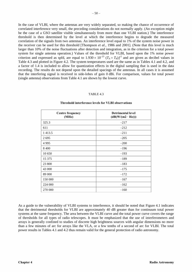
– 50 –
Chapter 4 Radio Astronomy
In the case of VLBI, where the antennas are very widely separated, so making the chance of occurrence of
correlated interference very small, the preceding considerations do not normally apply. (An exception might
be the case of a GSO satellite visible simultaneously from more than one VLBI station.) The interference
threshold is then determined by the level at which the interference begins to degrade the measured
correlation of the signals from two antennas. An interference level equal to 1% of the system noise power in
the receiver can be used for this threshold [Thompson et al., 1986 and 2001]. (Note that this level is much
larger than 10% of the noise fluctuations after detection and integration, as in the criterion for a total power
system for single antenna operation.) Values of the threshold for VLBI, based upon the 1% noise power
criterion and expressed as spfd, are equal to 1.930 10–23
(TA TR) f 2 and are given as decibel values in
Table 4.3 and plotted in Figure 4.2. The system temperatures used are the same as in Tables 4.1 and 4.2, and
a factor of 1.4 is included to allow for quantization effects in the digital sampling that is used in the data
recording. The results do not depend upon the detailed spacings of the antennas. In all cases it is assumed
that the interfering signal is received in side-lobes of gain 0 dBi. For comparison, values for total power
(single antenna) observations from Table 4.1 are shown by the lowest curve.
TABLE 4.3
Threshold interference levels for VLBI observations
As a guide to the vulnerability of VLBI systems to interference, it should be noted that Figure 4.1 indicates
that the detrimental thresholds for VLBI are approximately 40 dB greater than for continuum total power
systems at the same frequency. The area between the VLBI curve and the total power curve covers the range
of thresholds for all types of radio telescopes. It must be emphasized that the use of interferometers and
arrays is generally confined to studies of discrete high brightness sources with angular dimensions no more
than a few minutes of arc for arrays like the VLA, or a few tenths of a second of arc for VLBI. The total
power results in Tables 4.1 and 4.2 thus remain valid for the general protection of radio astronomy.
Centre frequency
(MHz)
Detrimental level
(dB(W/(m2 · Hz)))
325.3 –217
611 –212
1 413.5 –211
2 695 –205
4 995 –200
8 400 –196
10 650 –193
15 375 –189
23 800 –183
43 000 –175
89 000 –172
150 000 –167
224 000 –162
270 000 –160
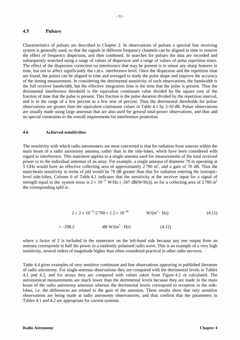
- 51 -
Radio Astronomy Chapter 4
– 5
1 –
4.5 Pulsars
Characteristics of pulsars are described in Chapter 2. In observations of pulsars a spectral line receiving
system is generally used, so that the signals in different frequency channels can be aligned in time to remove
the effect of frequency dispersion, and then combined. In searches for pulsars the data are recorded and
subsequently searched using a range of values of dispersion and a range of values of pulse repetition times.
The effect of the dispersion correction on interference that may be present is to smear any sharp features in
time, but not to affect significantly the r.m.s. interference level. Once the dispersion and the repetition time
are found, the pulses can be aligned in time and averaged to study the pulse shape and improve the accuracy
of the timing measurement. In considering the detrimental sensitivity of such observations, the bandwidth is
the full receiver bandwidth, but the effective integration time is the time that the pulse is present. Thus the
detrimental interference threshold is the equivalent continuum value divided by the square root of the
fraction of time that the pulse is present. This fraction is the pulse duration divided by the repetition interval,
and is in the range of a few percent to a few tens of percent. Thus the detrimental thresholds for pulsar
observations are greater than the equivalent continuum values in Table 4.1 by 2-10 dB. Pulsar observations
are usually made using large antennas that are also used for general total-power observations, and thus add
no special constraints to the overall requirements for interference protection.
4.6 Achieved sensitivities
The sensitivity with which radio astronomers are most concerned is that for radiation from sources within the
main beam of a radio astronomy antenna, rather than in the side-lobes, which have been considered with
regard to interference. This statement applies to a single antenna used for measurements of the total received
power or to the individual antennas of an array. For example, a single antenna of diameter 70 m operating at
5 GHz would have an effective collecting area of approximately 2 700 m2, and a gain of 70 dB. Thus the
main-beam sensitivity in terms of pfd would be 70 dB greater than that for radiation entering the isotropic-
level side-lobes. Column 6 of Table 4.1 indicates that the sensitivity at the receiver input for a signal of
strength equal to the system noise is 2 10–27
W/Hz (–267 dB(W/Hz)), so for a collecting area of 2 700 m2
the corresponding spfd is:
2 2 10–27
/2 700 1.5 10–30
W/(m2 · Hz) (4.11)
= –298.2 dB W/(m2 · Hz) (4.12)
where a factor of 2 is included in the numerator on the left-hand side because any one output from an
antenna corresponds to half the power in a randomly polarised radio wave. This is an example of a very high
sensitivity, several orders of magnitude higher than often considered practical in other radio services.
Table 4.4 gives examples of very sensitive continuum and line observations appearing in published literature
of radio astronomy. For single-antenna observations they are compared with the detrimental levels in Tables
4.1 and 4.2, and for arrays they are compared with values taken from Figure 4.2 or calculated. The
astronomical measurements are much lower than the detrimental levels because they are made in the main
beam of the radio astronomy antennas whereas the detrimental levels correspond to reception in the side-
lobes, i.e. the differences are related to the gain of the antennas. These results show that very sensitive
observations are being made at radio astronomy observatories, and thus confirm that the parameters in
Tables 4.1 and 4.2 are appropriate for current systems.
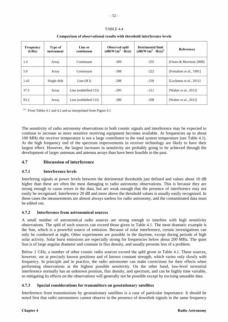
– 52 –
Chapter 4 Radio Astronomy
TABLE 4.4
Comparison of observational results with threshold interference levels
The sensitivity of radio astronomy observations to both cosmic signals and interference may be expected to
continue to increase as more sensitive receiving equipment becomes available. At frequencies up to about
100 MHz the receiver temperature is not a large contributor to the total system temperature (see Table 4.1).
At the high frequency end of the spectrum improvements in receiver technology are likely to have their
largest effect. However, the largest increases in sensitivity are probably going to be achieved through the
development of larger antennas and antenna arrays than have been feasible in the past.
4.7 Discussion of interference
4.7.1 Interference levels
Interfering signals at power levels between the detrimental thresholds just defined and values about 10 dB
higher than these are often the most damaging to radio astronomy observations. This is because they are
strong enough to cause errors in the data, but are weak enough that the presence of interference may not
easily be recognized. Interference 20 dB and more above the threshold values is usually easily recognized. In
these cases the measurements are almost always useless for radio astronomy, and the contaminated data must
be edited out.
4.7.2 Interference from astronomical sources
A small number of astronomical radio sources are strong enough to interfere with high sensitivity
observations. The spfd of such sources can exceed those given in Table 4.1. The most dramatic example is
the Sun, which is a powerful source of emission. Because of solar interference, certain investigations can
only be conducted at night. Other experiments are possible in the daytime, except during periods of high
solar activity. Solar burst emissions are especially strong for frequencies below about 200 MHz. The quiet
Sun is of large angular diameter and constant in flux density, and usually presents less of a problem.
Below 1 GHz, a number of other cosmic radio sources exceed the spfd given in Table 4.1. These sources,
however, are at precisely known positions and of known constant strength, which varies only slowly with
frequency. In principle and in practice, the radio astronomer can make corrections for their effects when
performing observations at the highest possible sensitivity. On the other hand, low-level terrestrial
interference normally has an unknown position, flux density, and spectrum, and can be highly time variable,
so mitigating its effects on the observations will generally not be possible except by excising unusable data.
4.7.3 Special considerations for transmitters on geostationary satellites
Interference from transmissions by geostationary satellites is a case of particular importance. It should be
noted first that radio astronomers cannot observe in the presence of downlink signals in the same frequency
Frequency
(GHz)
Type of
instrument
Line or
continuum
Observed spfd
(dB(W/(m2 · Hz)))
Detrimental limit
(dB(W/(m2 · Hz)))1 References
1.4 Array Continuum –309 –255 [Owen & Morrison 2008]
5.0 Array Continuum –308 –222 [Fomalont et al., 1991]
1.42 Single dish Line (H I) –288 –239 [Lockman et al., 2011]
37.3 Array Line (redshifted CO) –295 –211 [Walter et al., 2012]
93.2 Array Line (redshifted CO) –289 –208 [Walter et al., 2012]
(1) From Tables 4.1 and 4.2 and as interpolated from Figure 4.1

- 53 -
Radio Astronomy Chapter 4
– 5
3 –
band. Thus, considerations of interference from satellites are generally concerned with unwanted emissions
that fall within radio astronomy bands.
Because the power levels in Tables 4.1 and 4.2 are calculated assuming 0 dBi antenna gain, detrimental
interference will be encountered when antenna side-lobes of gain greater than 0 dBi are pointed towards a
transmitter radiating at the levels indicated in Tables 4.1 and 4.2. For a radio astronomy antenna with side-
lobes equal to those of the reference antenna defined in equation (4.1), interference would occur if the
antenna were pointed at an angle of 19 or less to the direction of a satellite radiating at these levels. Thus a
series of similar satellites located at intervals around the geostationary orbit would preclude radio astronomy
observations with high sensitivity from a band of sky 38 or more wide, centred on the orbit. The loss of
such a large area of sky would impose severe restrictions on radio astronomy observations.
A useful criterion for the protection of radio astronomy from geostationary satellite emissions is suggested in
Figure 4.3. This Figure shows the projection of the geostationary orbit in celestial coordinates as viewed
from the latitudes of a number of major radio astronomy observatories. If it were possible to point a radio
telescope to within 5 of the orbit without encountering detrimental interference, then for that telescope a
band of sky 10 wide would be unavailable for high-sensitivity observations. For a given observatory this
would still be a serious loss. However, for a combination of radio telescopes located at northern and southern
latitudes, operating at the same frequencies, the entire sky would be accessible. A value of 5 should
therefore be regarded as the requirement for minimum angular spacing between the main beam of a radio
astronomy antenna and the geostationary orbit.
FIGURE 4.3
Projection of the geostationary orbit on the celestial sphere as seen from a number
of radio observatories
Radio-Astro_43Hour angle (h)
Dec
lin
atio
n a
ng
le (
degre
es)
Radioastronomystations
Parkes
Itapetinga
Arecibo
VLANobevamaOVRONRAOAlgonquinBonnWesterborkOnsala
–6–9
–6
–5
–8
–7
–5
–4 –3 –2 –1 0 1 2 3 4 5 6
–4
–3
–2
–1
0
1
2
3
4
5
6

– 54 –
Chapter 4 Radio Astronomy
In the model antenna response in equation (4.1), the side-lobe level at an angle of 5 from the main beam is
15 dBi. Thus, to avoid detrimental interference to a radio telescope pointed 5 from the transmitter, the
satellite emissions within radio astronomy bands should be reduced 15 dB below the pfd’s given in Tables
4.1 and 4.2. When satellites are spaced at intervals of only a few degrees along the orbit, the e.i.r.p. levels of
the individual transmissions in the direction of an observatory must be even lower to meet the requirement
that the sum of the powers of all the interfering signals received should be 15 dB below PH in Tables 4.1
and 4.2.
It is clear that some further degree of protection from satellite emissions can be achieved by minimization of
the level of side-lobe gain near the main beam. This should be an important consideration in the design of
future radio astronomy antennas.
4.7.4 Filtering
Unwanted signal energy outside the pass-band of a radio astronomy receiver is rejected by using bandpass
filters. Several filters may be inserted at different stages in the receiving system to ensure that at no point are
the unwanted signals sufficiently strong to cause nonlinearity. Very high selectivity can be obtained by using
digital filters, but these must be preceded by sufficient amplification that the signals can be digitized. The
response at the band edges may need to be as low as –100 dB relative to the band center, so the width of the
filter at the –3 dB points may be less than the full width of the assigned band. Since intermediate frequencies
are relatively low, typically between 100 MHz and 10 GHz, relatively steep filter edges are possible. The
slope of the edges of the filter response depends upon the number of filter sections and the designed
response. Some further discussion of filtering is given in Chapter 6.
4.7.5 Interference levels capable of damaging or saturating a radioastronomy receiver
ITU-R Report RA. 2188 – Power flux-density and e.i.r.p. levels potentially damaging to radio astronomy
receivers, notes that input powers of order 25 mW will suffice to damage or destroy most radio astronomy
receivers while much weaker input levels will suffice to saturate their gain. There are several scenarios
involving existing radars that could lead to input of such power levels.
– Main-beam to main-beam coupling. The high gain of radio astronomy antennas, combined with the
high power and small spot sizes of various orbiting earth-sensing radars operating at frequencies
between 1 and 94 GHz represent such a possibility [SFCG Ref], should the main beams of both
systems ever overlap. Although such coupling is expected to be quite rare in a statistical sense, the
consequences to a radio astronomy operator of such an encounter would be quite dire.
– Main-beam to side-lobe coupling. As noted in ITU-R Recommendation 1750 – Mutual planning
between the Earth exploration-satellite service (active) and the radio astronomy service in the 94
GHz and 130 GHz bands, a radio astronomy receiver will saturate whenever the antenna on which it
is mounted is directly illuminated by a high-power earth-sensing orbiting radar, even for reception in
a 0 dBi sidelobe of the radio astronomy antenna. Conversely, the radio astronomy receiver will
saturate when the main beam of the radio astronomy antenna is illuminated by a 0 dBi or even
weaker sidelobe of an orbiting radar, given that the gain of a radio astronomy antenna is higher than
that of the orbiting radar.
Even rather modest transmitters like the 76-77 GHz and 77-81 GHz vehicular radars described in
Recommendation ITU-R M. 1452 – Millimetre wave vehicular collision avoidance radars and
radiocommunication systems for intelligent transport system applications, may produce saturating or
damaging power levels when operated in proximity to a radio astronomy antenna, given the high gain and
small spot sizes that accrue to the frequencies at which they operate.
4.8 Monte Carlo analysis
Monte Carlo analysis is sometimes used to estimate the fraction of time that an interfering signal will exceed
the detrimental threshold for radio astronomy. This procedure is useful in cases where the angle between the
direction of the interfering source and the main beam of the radio telescope varies rapidly. The variation can
result from the motion of the interfering source, as in the case of a non-GSO satellite, and/or the variation in
telescope pointing required by the astronomical program. The number and distance of active interfering
sources can also vary, as in the case of interference from ground-based mobile vehicles. In Monte Carlo
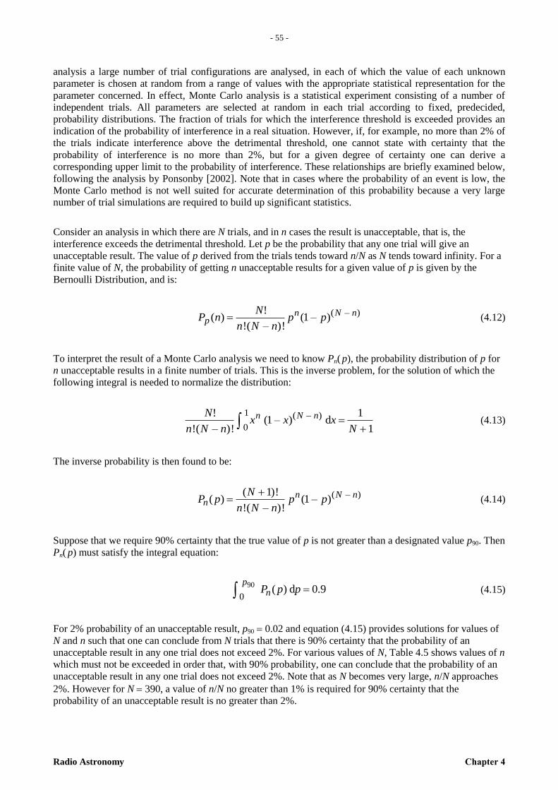
- 55 -
Radio Astronomy Chapter 4
– 5
5 –
analysis a large number of trial configurations are analysed, in each of which the value of each unknown
parameter is chosen at random from a range of values with the appropriate statistical representation for the
parameter concerned. In effect, Monte Carlo analysis is a statistical experiment consisting of a number of
independent trials. All parameters are selected at random in each trial according to fixed, predecided,
probability distributions. The fraction of trials for which the interference threshold is exceeded provides an
indication of the probability of interference in a real situation. However, if, for example, no more than 2% of
the trials indicate interference above the detrimental threshold, one cannot state with certainty that the
probability of interference is no more than 2%, but for a given degree of certainty one can derive a
corresponding upper limit to the probability of interference. These relationships are briefly examined below,
following the analysis by Ponsonby [2002]. Note that in cases where the probability of an event is low, the
Monte Carlo method is not well suited for accurate determination of this probability because a very large
number of trial simulations are required to build up significant statistics.
Consider an analysis in which there are N trials, and in n cases the result is unacceptable, that is, the
interference exceeds the detrimental threshold. Let p be the probability that any one trial will give an
unacceptable result. The value of p derived from the trials tends toward n/N as N tends toward infinity. For a
finite value of N, the probability of getting n unacceptable results for a given value of p is given by the
Bernoulli Distribution, and is:
)–()–1(
!)–(!
!)( nNn
p ppnNn
NnP (4.12)
To interpret the result of a Monte Carlo analysis we need to know Pn( p), the probability distribution of p for
n unacceptable results in a finite number of trials. This is the inverse problem, for the solution of which the
following integral is needed to normalize the distribution:
1
1d)–1(
!)–(!
! )(1
0
Nxxx
nNn
N nNn (4.13)
The inverse probability is then found to be:
)–()–1(
!)–(!
!)1()( nNn
n ppnNn
NpP
(4.14)
Suppose that we require 90% certainty that the true value of p is not greater than a designated value p90. Then
Pn( p) must satisfy the integral equation:
90
09.0d)(
pn ppP (4.15)
For 2% probability of an unacceptable result, p90 0.02 and equation (4.15) provides solutions for values of
N and n such that one can conclude from N trials that there is 90% certainty that the probability of an
unacceptable result in any one trial does not exceed 2%. For various values of N, Table 4.5 shows values of n
which must not be exceeded in order that, with 90% probability, one can conclude that the probability of an
unacceptable result in any one trial does not exceed 2%. Note that as N becomes very large, n/N approaches
2%. However for N 390, a value of n/N no greater than 1% is required for 90% certainty that the
probability of an unacceptable result is no greater than 2%.
– 56 –
Chapter 4 Radio Astronomy
TABLE 4.5
Values of N and n for no more than 2% probability of
an unacceptable result, with 90% certainty
ANNEX 1
TO CHAPTER 4
Side-lobe model from Recommendation ITU-R S.1428
The side-lobe gain model from Recommendation ITU-R S.1428, for antennas of diameter, D, greater than
100 wavelengths, , is as follows:
G() Gmax – 2.5 10–3
{D/λ}2 dBi for 0 m
G() G1 for φm r
G() 29 –25 log() dBi for r 10°
G() 34 – 30 log() dBi for 10 34.1
G() –12 dBi for 34.1 80
G() –7 dBi for 80 120
G() –12 dBi for 120 180
where:
Gmax 10 log{(D/λ)2} dBi
: aperture efficiency for 0.7, Gmax 20 log{D/λ} 8.4 dBi
G1 –1 15 log{D/λ} dBi
m {20λ/D}(Gmax – G1)1/2
degrees
r 15.85 {D/λ}–0.6
degrees
N n n/N
(%)
p90
(%)
292 1 0.52 2.0
397 4 1.01 2.0
776 10 1.29 2.0
1 900 30 1.58 2.0
10 000 181 1.81 2.0
50 000 960 1.92 2.0
- 57 -
Radio Astronomy Chapter 4
– 5
7 –
REFERENCES
BARNBAUM, C. and BRADLEY, R. F. [1998] A new approach to interference excision in Radio
Astronomy: real-time adaptive cancellation. Astron. J., Vol. 116, p. 2598-2614.
CCIR [1966] Report 224-1. Documents of the XIth Plenary Assembly, ITU, Geneva, Vol. IV, p. 537-548.
ELLINGSON, S. W. and CAZEMIER, W. [February 2003] Efficient multibeam synthesis with interference
nulling for large arrays. IEEE Trans. Ant. Prop.
FOMALONT, E. B. et al. [1991] The micro-jansky radio source population at 5 GHz. Astron. J., Vol. 102,
p. 1258-1277.
KRAUS, J. D. [1966] Radio Astronomy. McGraw Hill, New York, NY, Second ed. 1986, Cygnus-Quasar
Books, Powell, OH.
LOCKMAN, F. J., FREE, N. L. and SHIELDS, J. C. [2012] The Neutral Hydrogen Bridge Between M31
and M33, Astron. J., Vol. 144, p. 52 – 67.
OWEN, F. and MORRISON, G. E., [2008] The Deep Swire Field I. 20 cm Continuum Radio Observations:
A Crowded Sky, Astron.. J., Vol. 136, p. 1889-1900.
PONSONBY, J. E. B. [10-14 June 2002] On 2% by Monte Carlo, Proc. of IUCAF Summer School In
Spectrum Management And Frequency Coordination, NRAO, Green Bank, West Virginia.
Planck Collaboration et. al [2011] Planck early results. I. The Planck Mission, Astron. and Astrophys, Vol.
536, 1
SFCG: information available at https://www.sfcgonline.org
SMOOT, G. et al. [1992] Structure in the COBE differential microwave radiometer first-year maps.
Astrophys. J. (Letters), Vol. 396, L1-L5.
THOMPSON, A. R. [1982] The response of a radio-astronomy synthesis array to interfering signals, IEEE
Trans. Ant. Prop., Vol. AP-30, p. 450-456.
THOMPSON, A. R., MORAN, J. M. and SWENSON, G. W. Jr. [1986 and 2001] Interferometry and
synthesis in radio astronomy. John Wiley, New York, NY, reprinted by Krieger Press, Melbourne, FL., see
Chapter 14. Second ed., John Wiley, 2001, see Chapter 15.
WALTER, F. et al [2012] Nature, The intense starburst HDF 850.1 in a galaxy overdensity at z ≈ 5.2 in the
Hubble Deep Field, Vol. 486, p 233-238.
– 58 –
Chapter 5 Radio Astronomy
CHAPTER 5
Sharing the radio astronomy bands with other services
5.1 General remarks
Most radio astronomy bands are shared with active services, which transmit. Such sharing is particularly
difficult for radio astronomy, which is a passive service and is very sensitive to interference. Because of the
great distances of astronomical sources, the pfd levels of the emissions under investigation are often 100 dB
or more below those of man-made transmissions near the radio observatory. The strength and characteristics
of the astronomical signals are determined by laws of nature and are beyond the control of the radio
astronomer. Furthermore, because of the experimental nature of the science the radio astronomer is often
unable to know in advance what the characteristics of the emissions will be. These factors make radio
astronomy particularly vulnerable to interference. Interference can be damaging not only if it is strong and
obliterates the astronomical signals, but also if it is weak. An insidious danger to radio astronomy lies in the
interference which is just below the power level at which it can be recognized in individual measurements,
and which is present for a large fraction of the total time. In this case there may be no means during the
experiment of detecting that interference has occurred, and the subsequent results could contain serious
errors.
Radio astronomy observatories are usually located at sites specially chosen to minimize interference from
other services. The sites are usually at a considerable distance from the major terrestrial sources of
interference and, when not observing at mm-wavelengths, where it is important to get above as much of the
atmosphere as possible, are frequently screened by nearby high ground. With this protection for the
observatory, and the protection afforded by the curvature of the Earth, sharing with terrestrial transmitters is
possible when the transmitter power is low and there is sufficient geographical separation. However, with the
very sensitive systems used in radio astronomy, large separations are usually necessary. It is shown in § 5.3
that sharing is not generally possible when the transmitter is within LoS of the radio astronomy antenna or
the antenna feed. It is usually necessary for the transmitter to lie well over the horizon, at distances of 100
km or more. Transmitters carried in aircraft, spacecraft, high altitude platform stations or balloons can
remain within LoS of an observatory for very great distances, and the advantages associated with a carefully
selected observatory site and attenuation due to curvature of the Earth are both lost. At HF (3-30 MHz) any
interference received is almost invariably propagated via the ionosphere. In this case, the selection of the
observatory site and the curvature of the Earth do not provide protection, and in some circumstances
interference can be expected from a co-channel transmitter anywhere on the Earth.
A useful distinction can be drawn between local, regional and global sharing problems. A local problem such
as interference caused by a transmitter near a radio observatory will need to be solved at a local level, taking
factors such as site shielding into account. Regional problems, such as the interference caused by television
transmitters, have to be addressed on a regional scale, taking into account national frequency plans and other
regional factors; for example the different conditions and frequency assignments in countries that are
geographically close together. Global problems such as the interference caused by satellite-borne transmitters
can only be solved at the ITU level. Each class of sharing problem requires its own type of solution.
5.1.1 Protection criteria for the RAS
An important protection criterion for radio astronomy is the power level of the interference considered
harmful. The harmful threshold depends on the frequency of observation and the type of measurement being
made, as discussed in Chapter 4. The detailed characteristics of the interference may also need to be taken
into account.
A second criterion relates to the fraction of the sky over which radio astronomy observations are to be
protected. For ground-based sources of interference a value of 0 dBi is adopted for the gain of the radio
astronomy antenna in the direction of the interfering source, or in the direction of the horizon for a distant
transmitter. The adoption of this value means that potential sources of interference at the harmful threshold
- 59 -
Radio Astronomy Chapter 5
– 5
9 –
levels given in Recommendation ITU-R RA.769 will not cause detrimental interference to observations
made at elevation angles greater than 19 (based on the model radiation pattern given in Recommendation
ITU-R SA.509). Observations made below 19 elevation will suffer interference if transmissions from the
(terrestrial) interfering source are received through side-lobes with gain greater than 0 dBi. In this case, part
of the sky is effectively blocked for radio astronomy observations, as explained in Annex 1 to
Recommendation ITU-R RA.1513. In fact radio astronomers may be prepared to accept this restriction of
their sky coverage, because Earth rotation will allow most celestial objects to be accessed at a more
favourable elevation angle. However, such sky blockage can be very restrictive for observations of celestial
sources which make only a brief appearance above the horizon (for example, observations of the galactic
centre from high northerly latitudes), or for time-critical observations. For interference from geostationary
spacecraft a value of 12-15 dBi for the gain of the radio astronomy antenna is desirable to allow observations
to be made to within 5 of a satellite in the geostationary orbit, as discussed in Chapter 4. The application of
the concept of sky blockage to cases of interference from transmitters on aircraft of spacecraft in non-
geostationary orbit is described in Recommendations ITU-R S.1586 and ITU-R M.1583.
A third criterion that must be considered is the percentage-of-time that a threshold interference level may be
exceeded without seriously degrading the operation of the service. The percentage-of-time criterion and the
related issue of sky blockage are considered in Recommendation ITU-R RA.1513, which specifies an
aggregate data loss of 5% from transmitters in all services, in any frequency band allocated to the RAS on a
primary basis, and no more than 2% data loss from transmitters in any one service. It is noted that the
concept of aggregate data loss is not fully developed yet and further studies of the apportionment of
interference between different networks and services is needed. Recommendation ITU-R RA.1513 also
specifies that the percentage of data loss is to be determined as the percentage of integration periods of 2 000
s in which the average spfd at the radio telescope exceeds the levels defined in Recommendation ITU-R
RA.769 (assuming 0 dBi antenna gain). The effect of interference that is periodic on timescales of the order
of seconds or less requires further study.
It must be emphasized that for some types of observation a 5% failure rate due to interference imposes
severe restrictions on the radio astronomer. For some observations, such as those of a comet, an occultation
by the moon, or a supernova explosion, a high probability of success is desirable because of the difficulty or
impossibility of repeating them. Other types of observation require simultaneous measurements at different
wavelengths and at a number of sites, at each of which success must be obtained if the experiment as a whole
is to be successful. An example is a coordinated multi-wavelength study of a flaring nova. Such an
experiment may be severely damaged if observations at any one of the observatories are unusable because of
interference. An observatory having difficulties of this type would require special national arrangements at
certain frequencies at certain times.
Another propagation effect to consider is reflection of the interfering signal. Reflections from aircraft are
likely causes of interference in a shared band even when the terrestrial transmitter is distant. The possibility
of interference by reflection from low-orbit satellites also exists. A single reflecting body will be effective
for only a short time and the interference problem will depend on the density of air or space traffic. A
problem is that, as a result of space activities, there are a large number of metallic objects in orbit around the
Earth. For certain types of radio astronomical measurement in shared bands, reflections of terrestrial
transmissions by the Moon can cause serious interference.
The protection criteria so far considered have involved the power threshold of interference, the percentage of
sky to be protected, and the fraction of observing time which is to be protected. These all relate directly to
geographical sharing, that is, the geographical spacing of two services which enables both to work at the
same frequency at the same time. In sharing between some services, additional protection may be obtained
by the use of orthogonal polarisations. This is not a useful technique for protecting radio astronomy since
both polarisations must be used for many observations, and also since the interference generally enters the
radio astronomy system through far side-lobes of a high-gain antenna with polarisation characteristics very
different from those of the main beam.
It should be noted that, except in rare cases, sharing with the RAS is possible only with effective
geographical separation. Limited time-sharing to permit special observations at a radio astronomy site may
be possible, and may indeed be necessary on occasion, as discussed in § 5.9. In particular, this may be useful
in bands not allocated to radio astronomy.
– 60 –
Chapter 5 Radio Astronomy
5.2 Separation distances required for sharing with a single transmitter (see Recom-
mendation ITU-R RA.1031)
If geographical sharing is to be successful, the interfering transmitter and the interfered-with receiver must
be separated by a distance at which the interference is not considered harmful. For the criteria developed in
Chapter 4, the attenuation over this distance must be sufficient to reduce the interfering signal below the
appropriate level in Recommendation ITU-R RA.769, for all but a percentage, p%, of the time. RR Appendix
7 defines transmission loss Lb( p). This equation is given below, with the addition of an Atmospheric
attenuation term, A:
Lb( p) Pt Gt Gr – Pr ( p) - A(5.1)
where:
Lb( p) : minimum permissible basic transmission loss (dB) for p% of the time; this value must be
exceeded by the actual transmission loss for all but p% of the time
Pt : transmitting power level (dBW) in the reference bandwidth at the input to the antenna
Gt : gain (dBi) of the transmitting antenna in the direction of the radio astronomy antenna
Gr : gain (dBi) of the radio astronomy antenna in the direction of the transmitter
Pr ( p) : maximum permissible interference power (dBW) in the reference bandwidth to be
exceeded for no more than p% of time at the receiver input
A: the additional loss factor due to atmospheric absorption.
Using the protection criteria of Chapter 4, Gr 0 dBi and equation (5.1) assumes the form:
Lb( p) Pt Gt – Pr ( p) - A (5.2)
where Pr is to be taken from column 7 of Table 4.1 or Table 4.2 of Chapter 4. Lb( p) should be calculated
using an appropriate model, such as in the comprehensive set given in Recommendations ITU-R P.452,
ITU-R P.526 and ITU-R P.617.
Atmospheric attenuation increases rapidly with increasing humidity and observing frequency. Below
15 GHz, the zenith atmospheric attenuation is often small, < 0.1 dB and may be ignored in equation (5.2).
Between 15 and 115 GHz, the zenith opacity at high dry sites is modest, < 1 dB, and provides only small
interference protection. Above 115 GHz the atmospheric opacity varies rapidly near the resonant frequencies
of molecules in the atmosphere, and provides significant interference protection (see § 5.7).
For LoS transmission the free-space transmission loss is not generally variable and the percentage-of time-
criterion is not pertinent. In this case Lb has a simple analytical form and equation (5.2) may be written as:
20 log(4d ) – 20 log() Pt Gt – Pr - A (5.3)
where d is the distance (m) between transmitter and receiver and is the wavelength (m).
In the above analysis Pt is the power transmitted within the bandwidth Br of the radio astronomy receiver. If
the transmitter power PT is distributed over a bandwidth Bt Br then:
Pt PT – 10 log(Bt / Br) + A (5.4)
assuming that the transmitter power has a uniform spectral density.
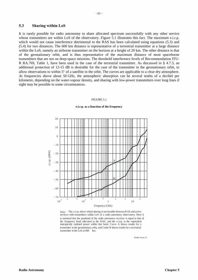
- 61 -
Radio Astronomy Chapter 5
– 6
1 –
5.3 Sharing within LoS
It is rarely possible for radio astronomy to share allocated spectrum successfully with any other service
whose transmitters are within LoS of the observatory. Figure 5.1 illustrates this fact. The maximum e.i.r.p.
which would not cause interference detrimental to the RAS has been calculated using equations (5.3) and
(5.4) for two distances. The 600 km distance is representative of a terrestrial transmitter at a large distance
within the LoS, namely an airborne transmitter on the horizon at a height of 20 km. The other distance is that
of the geostationary orbit, and is thus representative of the maximum distance of most spaceborne
transmitters that are not on deep-space missions. The threshold interference levels of Recommendation ITU-
R RA.769, Table 1, have been used in the case of the terrestrial transmitter. As discussed in § 4.7.3, an
additional protection of 12-15 dB is desirable for the case of the transmitter in the geostationary orbit, to
allow observations to within 5 of a satellite in the orbit. The curves are applicable to a clear dry atmosphere.
At frequencies above about 50 GHz, the atmospheric absorption can be several tenths of a decibel per
kilometre, depending on the water-vapour density, and sharing with low-power transmitters over long lines if
sight may be possible in some circumstances.
FIGURE 5.1
e.i.r.p. as a function of the frequency
Radio-Astro_51
Frequency (GHz)
e.i.
r.p. (
dB
W)
Note – The e.i.r.p. above which sharing is not feasible between RAS and active services with transmitters within LoS of a radio astronomy observatory. Here it
is assumed that the passband of the radio astronomy receiver is equal to that of the frequency band allocated to the RAS, and the e.i.r.p. is the equivalent isotropically radiated power within that band. Curve A shows results for a
transmitter in the geostationary orbit, and Curbe B shows results for a terrestrial transmitter in the LoS at 600 km.
20
10
0
– 10
– 50
– 60
– 20
– 30
– 40
– 70
10–2
10110–1
2 5 2 5 2 5 2
A
B
– 62 –
Chapter 5 Radio Astronomy
It is clear from Figure 5.1 that sharing with a LoS terrestrial transmitter is unlikely to be possible at
frequencies below 10 GHz because of the severe restriction sharing would impose on the transmitter e.i.r.p.
Even for frequencies up to 40 GHz, either the transmitter power must be no more than a few milliwatts, or
the transmitting antenna must provide high discrimination towards the direction of the observatory, for
sharing to be possible. For spaceborne transmitters not in deep-space, with typical power in excess of 1 W,
sharing will not be possible even outside the coverage area of the spaceborne antenna for frequencies up to
about 20 GHz. Between 20 GHz and 50 GHz sharing is not likely to be possible within the coverage area of
the spaceborne antenna. Transmitters on spacecraft at heights less than 6 400 km would need to be restricted
to an e.i.r.p. lying between curves A and B, for sharing to be possible.
A special case of sharing with spacecraft on deep-space missions is described in § 5.8.
5.4 Sharing with services with terrestrial transmitters
The establishment of coordination zones around radio astronomy sites provides a method of avoiding
detrimental interference from terrestrial transmitters of other services that share a radio astronomy band.
From the preceding discussion it is clear that sharing will only be possible for services whose transmitters are
beyond the horizon. The basic criterion used to define a coordination zone is that the total interference from
all users outside the zone must not exceed the harmful threshold level measured at the radio astronomy site.
Thus the size of the coordination zone depends on a number of factors. The types of measurements being
made at the radio astronomy site determine the corresponding interference thresholds given in
Recommendation ITU-R RA.769. The number and distribution of the users outside the zone, the e.i.r.p. of
the user transmissions in the direction of the radio astronomy site, the fraction of the time they are active, and
the propagation characteristics determine the interfering pfd at the radio astronomy site. The propagation
characteristics depend on factors such as the profile of the terrain, presence of trees, and the atmospheric
conditions. Appropriate propagation models are suggested in § 5.2.
Because of the many factors involved, the boundaries of the coordination zones need to be established
individually for each radio astronomy site at which such a zone is required, taking due account of any special
features of the radio astronomy measurements, and of the active service that shares the band. It should be
realized that the size of the coordination zone is likely to be 100 km or more. For many small countries the
coordination zone required may extend beyond the national boundaries into countries where the frequency
allocations are different. Thus special conditions may need to be applied when determining coordination
zones to protect radio astronomy in small countries.
The coordination zone defines a region around the radio observatory outside of which the users of the active
service can transmit freely without causing interference to the radio astronomy observations. For users within
the coordination zone technical means must be found to avoid detrimental interference to the RAS. For
example this could involve careful siting of a fixed transmitter to take advantage of natural shielding, or
designing the transmitting antenna to have a null in the direction of the observatory. In other cases the only
technical solution may be to avoid any transmissions in the radio astronomy band within the coordination
zone.
5.5 Sharing with mobile services
In principle coordination zones can be set up to protect radio astronomy sites from mobile transmitters. In
this case the mobile user must have some means of determining when a coordination zone has been entered,
and some means of reducing the interference received at the radio observatory to a level below the harmful
threshold. Recommendation ITU-R M.1316 sets out principles and a methodology for sharing between the
MSS (Earth-to-space) and the RAS in the bands 1 610.6-1 613.8 MHz and 1 660-1 660.5 MHz, based on a
Monte Carlo simulation approach. The method introduces, in addition to the coordination zone, an inner
exclusion zone where no mobiles may transmit, together with an intermediate restriction zone within which
there may be some restrictions to the operation of mobiles. However the validity of the Monte Carlo
approach as a basis for effective protection of radio astronomy has yet to be demonstrated in practice.
- 63 -
Radio Astronomy Chapter 5
– 6
3 –
For the case of mobile transmitters on aircraft the size of the coordination zone is much larger than for
ground-based transmitters. Aircraft are likely to remain within LoS of a radio observatory for great distances,
as discussed in § 5.3, and sharing is likely to be very difficult. Coordination zones of many hundreds of
kilometres will be needed in general, unless the radio astronomy site is exceptionally well shielded by an
elevated horizon.
5.6 Sharing in radio astronomy bands below 40 GHz
Table 5.1 gives the results of sharing calculations that have been made for shared radio astronomy bands
below 40 GHz (taken from ex-CCIR Report 696-2). The Table illustrates the wide range of sharing scenarios
for the RAS, and the large separation distances that are needed. For most bands a separation distance
necessary for sharing between a hypothetical transmitter and a radio astronomy receiver was calculated as
described in the previous sections. The separation distance providing the necessary basic transmission loss
depends on the propagation mechanism. For frequencies up to 38 MHz ionospheric effects dominate. For
higher frequencies tropospheric scatter is primarily responsible for interference at the 10% of time level. The
separation distances for frequencies 74 MHz to 408 MHz were calculated without the benefit of the latest
models (Recommendations ITU-R P.452, ITU-R P.526 and ITU-R P.617). It is estimated that the
propagation losses may be in error by approximately 10 dB, out of a total basic transmission loss of typically
220 dB. This in turn means that the separation distances may be in error by typically 50-100 km, when
compared with the results obtained using the latest propagation models. The distances for frequencies above
408 MHz were calculated using Recommendation ITU-R P.452-5. The radio astronomy antenna was
assumed throughout to have a height of 25 m. The results are not strongly dependent on this assumption.
Results are given for two cases, one a site with a horizon angle of 1, and the other a well-protected site with
a horizon angle of 4. Some particular frequency bands are discussed in greater detail below.
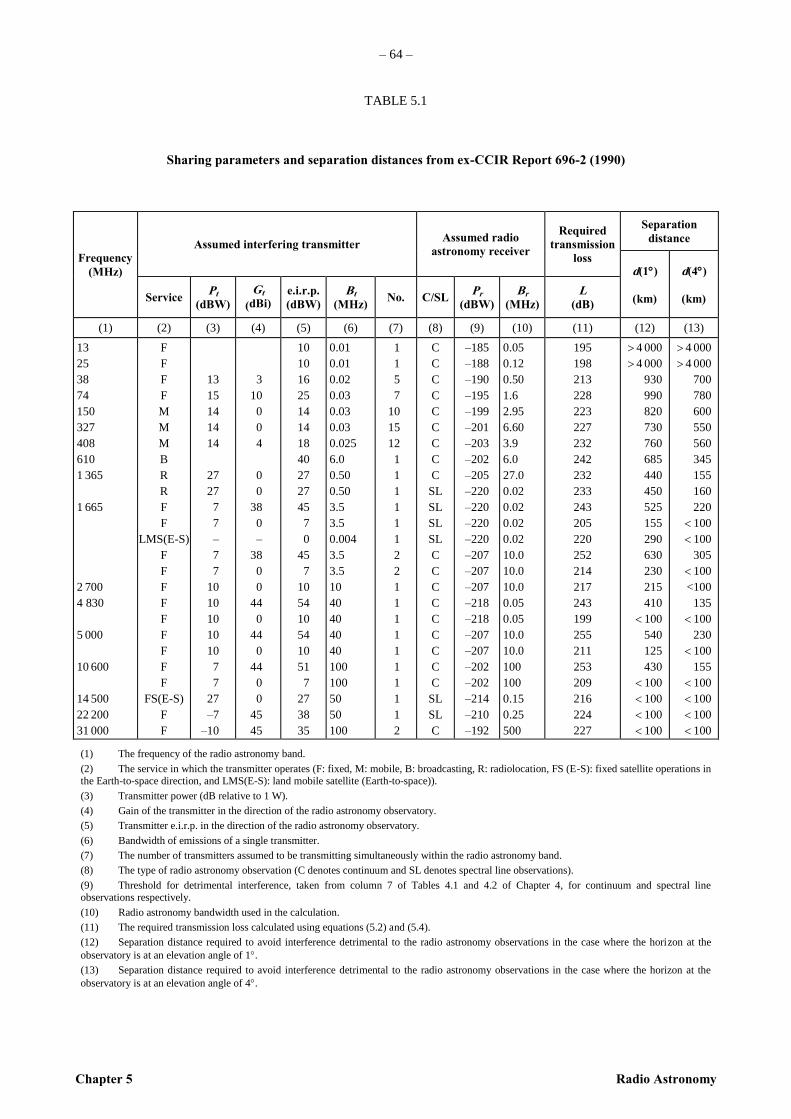
– 64 –
Chapter 5 Radio Astronomy
TABLE 5.1
Sharing parameters and separation distances from ex-CCIR Report 696-2 (1990)
Frequency
(MHz)
Assumed interfering transmitter Assumed radio
astronomy receiver
Required
transmission
loss
Separation
distance
d(1)
(km)
d(4)
(km) Service Pt
(dBW)
Gt
(dBi) e.i.r.p.
(dBW)
Bt
(MHz) No. C/SL
Pr
(dBW)
Br
(MHz)
L
(dB)
(1) (2) (3) (4) (5) (6) (7) (8) (9) (10) (11) (12) (13)
13
25
38
74
150
327
408
610
1 365
1 665
2 700
4 830
5 000
10 600
14 500
22 200
31 000
F
F
F
F
M
M
M
B
R
R
F
F
LMS(E-S)
F
F
F
F
F
F
F
F
F
FS(E-S)
F
F
13
15
14
14
14
27
27
7
7
–
7
7
10
10
10
10
10
7
7
27
–7
–10
3
10
0
0
4
0
0
38
0
–
38
0
0
44
0
44
0
44
0
0
45
45
10
10
16
25
14
14
18
40
27
27
45
7
0
45
7
10
54
10
54
10
51
7
27
38
35
0.01
0.01
0.02
0.03
0.03
0.03
0.025
6.0
0.50
0.50
3.5
3.5
0.004
3.5
3.5
10
40
40
40
40
100
100
50
50
100
1
1
5
7
10
15
12
1
1
1
1
1
1
2
2
1
1
1
1
1
1
1
1
1
2
C
C
C
C
C
C
C
C
C
SL
SL
SL
SL
C
C
C
C
C
C
C
C
C
SL
SL
C
–185
–188
–190
–195
–199
–201
–203
–202
–205
–220
–220
–220
–220
–207
–207
–207
–218
–218
–207
–207
–202
–202
–214
–210
–192
0.05
0.12
0.50
1.6
2.95
6.60
3.9
6.0
27.0
0.02
0.02
0.02
0.02
10.0
10.0
10.0
0.05
0.05
10.0
10.0
100
100
0.15
0.25
500
195
198
213
228
223
227
232
242
232
233
243
205
220
252
214
217
243
199
255
211
253
209
216
224
227
4 000
4 000
930
990
820
730
760
685
440
450
525
155
290
630
230
215
410
100
540
125
430
100
100
100
100
4 000
4 000
700
780
600
550
560
345
155
160
220
100
100
305
100
<100
135
100
230
100
155
100
100
100
100
(1) The frequency of the radio astronomy band.
(2) The service in which the transmitter operates (F: fixed, M: mobile, B: broadcasting, R: radiolocation, FS (E-S): fixed satellite operations in the Earth-to-space direction, and LMS(E-S): land mobile satellite (Earth-to-space)).
(3) Transmitter power (dB relative to 1 W).
(4) Gain of the transmitter in the direction of the radio astronomy observatory.
(5) Transmitter e.i.r.p. in the direction of the radio astronomy observatory.
(6) Bandwidth of emissions of a single transmitter.
(7) The number of transmitters assumed to be transmitting simultaneously within the radio astronomy band.
(8) The type of radio astronomy observation (C denotes continuum and SL denotes spectral line observations).
(9) Threshold for detrimental interference, taken from column 7 of Tables 4.1 and 4.2 of Chapter 4, for continuum and spectral line observations respectively.
(10) Radio astronomy bandwidth used in the calculation.
(11) The required transmission loss calculated using equations (5.2) and (5.4).
(12) Separation distance required to avoid interference detrimental to the radio astronomy observations in the case where the horizon at the
observatory is at an elevation angle of 1.
(13) Separation distance required to avoid interference detrimental to the radio astronomy observations in the case where the horizon at the
observatory is at an elevation angle of 4.
- 65 -
Radio Astronomy Chapter 5
– 6
5 –
5.6.1 The band 1 330-1 427 MHz
The region of the frequency spectrum in the vicinity of the 21 cm wavelength spectral-line of hydrogen is of
very great importance to radio astronomy. This importance has been recognized by the world-wide allocation
to radio astronomy, in the exclusively passive band 1 400 MHz to 1 427 MHz for both line and continuum
observations. Over the years, observations of the hydrogen spectral-line, Doppler-shifted to lower
frequencies, have grown in importance. This shift to lower frequencies is the result of the large velocities at
which distant galaxies are moving away from our Galaxy. The importance of the observations is recognized
in footnote RR No. 5.149 which gives some protection to radio astronomy in a band below 1 400 MHz. In
this band radiolocation has primary status in Regions 2 and 3 and shares primary status with the fixed and
mobile services in Region 1.
A typical radiolocation system used for aeronautical purposes in this band is a ground-based radar with 500
kW peak pulse power and an antenna gain of 34 dBi. If the dynamic range of the radio astronomy receiver is
sufficient to accommodate the radar peak power, the important parameter, with respect to interference, is the
average power into the radio astronomy receiver during its integration time. For a radar scanning 360, the
average e.i.r.p. in the direction of the radio astronomy observatory is of the order of the average power from
the transmitter. The actual power so transmitted is a function of the radar antenna pattern and of the nature of
the scan. With the assumption that the radar has a duty cycle of 0.001, the average power is 500 W. For a
spectral line observation, Table 2 of Recommendation ITU-R RA.769 is used, and the detrimental
interference level is –220 dBW in a 20 kHz band. The radar output power of 500 W is assumed to be
distributed uniformly over 0.5 MHz (a 2 ms pulse). This reduces the power into a single channel of the radio
astronomy receiver by 10 log (500/20) 14 dB. The required basic transmission loss is then 233 dB, leading
to separation distances of 450 km and 160 km for horizon elevations of 1 and 4 respectively: see Table 5.1.
It must be noted that the peak power into the receiver input is 142 dBW when the average interference is
just at the detrimental threshold. This is about 15 dB above the receiver noise power in a 0.5 MHz band and,
particularly if more than one radar signal is in the passband of the receiver front end, non-linear effects may
invalidate the analysis in terms of average power.
5.6.2 The band 4 800-5 000 MHz
In the 4 800-4 990 MHz band, radio astronomy has a secondary allocation, while fixed and mobile services
have primary allocations. However, footnote RR No. 5.149 singles out the bands 4 825-4 835 MHz and
4 950-4 990 MHz for special treatment. The first of these bands is for the observation of a spectral line of
formaldehyde.
In the band 4 990-5 000 MHz, radio astronomy is on an equal primary basis with the fixed and mobile
(except aeronautical mobile) services. Fixed-service usage in this band may be either low power radio-relay
systems or tropospheric scatter systems. Because of the very high average power used in the latter systems,
sharing with radio astronomy is very difficult. The radio-relay systems with perhaps 10 W transmitter power,
40 MHz RF bandwidth and 44 dBi antenna gain present an easier sharing problem. Results are given in
Table 5.1 for two cases of radio-relay systems, one with an antenna pointing directly at the radio
observatory, and the other pointing away from the observatory (0 dBi gain in the direction of the
observatory).
5.6.3 The bands 22.01-22.21 and 22.21-22.5 GHz
In the first of these two bands, radio astronomy has no allocation but administrations are urged to protect
radio astronomy observations. In the second band, radio astronomy has a primary allocation. In both bands
the sharing is with fixed and mobile (except aeronautical mobile) services. The band contains an important
spectral line of water vapour at 22.235 GHz, and it is sharing with spectral-line observations that are
considered here. This spectral line of water can produce a powerful maser emission (a “megamaser”) from
around the massive black hole in the centre of an active galaxy, and can be detected at large Doppler-shifts
from the rest frequency [Greenhill et al., 2003]. Results are presented in Table 5.1 for the case of a fixed
services antenna that is pointing towards the radio observatory.
– 66 –
Chapter 5 Radio Astronomy
5.7 Sharing in radio astronomy bands above 40 GHz
There are allocations above 40 GHz to the RAS for both continuum and spectral line observations. Some of
these allocations are shared with a variety of active services. Until recently there have been relatively few
active systems operating above 40 GHz, and consequently few reported cases of interference to radio
astronomy. This situation is now changing, and sharing studies are being undertaken for several frequency
bands, including the band 42.5-43.5 GHz which is shared between the RAS, the fixed service, the FSS
(Earth-to-space) and the mobile service (except aeronautical). The fixed service applications include high
density fixed service applications, (see footnote RR 5.547). Sharing with active services above 40 GHz may
be easier than at lower frequencies for several reasons. Firstly, high transmitting directivity is easily achieved
at these frequencies with antennas of modest size; secondly, the atmospheric attenuation is higher at these
frequencies; and thirdly, the scattering of signals by the troposphere decreases with increasing frequency.
5.7.1 Sharing between 60 and 275 GHz
Recommendation ITU-R RA.1272 considers the protection of radio astronomy measurements above 60 GHz
from ground-based interference. There are special sharing difficulties unique to these high frequencies.
Millimetre wave receivers for radio astronomy are normally designed to cover the full width of the
atmospheric windows (68-116 GHz, 130-170 GHz, 200-323 GHz etc.), either to take advantage of the
information contained in many spectral lines, or to achieve high bandwidth for sensitive continuum
measurements. Furthermore the superconductor-insulator-superconductor mixers employed as first stages of
the extremely sensitive heterodyne receivers are highly susceptible to saturation or even destruction by
interfering signals from anywhere in the band that they cover, while low loss filter technology to protect
them is not yet available. On the positive side, however, there are only a relatively small number of mm
wave observatories to be protected worldwide, and they are located, whenever practicable, at isolated remote
locations, to take maximum advantage of extremely dry atmospheric conditions and low levels of ground-
based interference. Hence mm wave observatories may be protected effectively from ground-based
transmissions at all frequencies above 60 GHz by means of coordination zones of modest size, with minimal
disruption to ground-based services. Recommendation ITU-R RA.1272 recommends the establishment of
coordination zones around mm wave observatories for all frequencies above 60 GHz, where practicable. The
coordination zones are to be defined using the interference thresholds of Recommendation ITU-R RA.769
and the procedure outlined in Recommendation ITU-R RA.1031
5.7.2 Sharing above 275 GHz
Certain characteristics of the frequency range 275-3 000 GHz combine to reduce the likelihood of
interference between the radio astronomy service and active services in this range. In the range 275-3 000
GHz, propagation through the Earth’s atmosphere is strongly affected by absorption due to atmospheric
molecules. The molecular species most responsible for the absorption are oxygen (O2) and water vapor
(H2O). Non-resonant absorption creates a general continuum of absorption that steadily increases with
frequency, while exceedingly large values of attenuation are found at specific frequencies corresponding to
natural resonances of the molecules. At sea level, the general continuum of absorption is approximately 5
dB/km at 275 GHz, 300 dB/km at 1 000 GHz, and 4 000 dB/km at 3 000 GHz. At specific molecular
resonances in this range, the attenuation can be as high as 550 000 dB/km. Attenuation decreases with
altitude due to lower concentrations of oxygen and water vapor. Figure 5.2 shows attenuation in dB/km at
different altitudes: sea level, 1 000m and 3 000 m. The parameters used in the calculation of these curves are
given in Report ITU-R RA.2189.
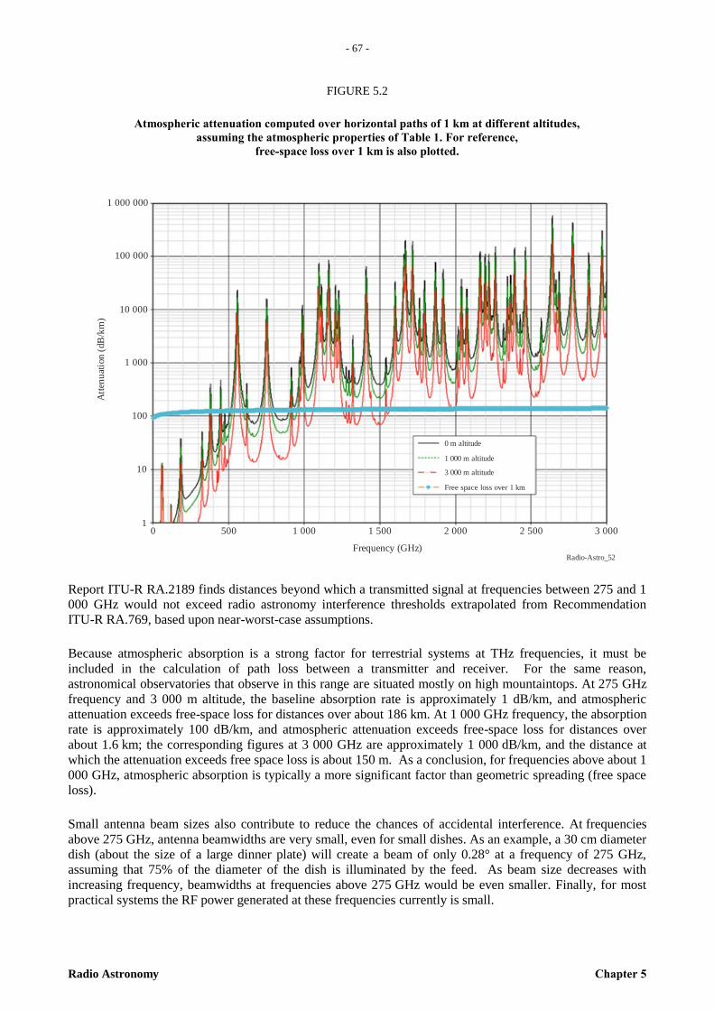
- 67 -
Radio Astronomy Chapter 5
– 6
7 –
FIGURE 5.2
Atmospheric attenuation computed over horizontal paths of 1 km at different altitudes,
assuming the atmospheric properties of Table 1. For reference,
free-space loss over 1 km is also plotted.
Radio-Astro_52
01
10
Frequency (GHz)
1 000 m altitude
Att
enu
atio
n (
dB
/km
)
500 1 000 1 500 2 000 2 500 3 000
1 000 000
100 000
10 000
1 000
100
0 m altitude
3 000 m altitude
Free space loss over 1 km
Report ITU-R RA.2189 finds distances beyond which a transmitted signal at frequencies between 275 and 1
000 GHz would not exceed radio astronomy interference thresholds extrapolated from Recommendation
ITU-R RA.769, based upon near-worst-case assumptions.
Because atmospheric absorption is a strong factor for terrestrial systems at THz frequencies, it must be
included in the calculation of path loss between a transmitter and receiver. For the same reason,
astronomical observatories that observe in this range are situated mostly on high mountaintops. At 275 GHz
frequency and 3 000 m altitude, the baseline absorption rate is approximately 1 dB/km, and atmospheric
attenuation exceeds free-space loss for distances over about 186 km. At 1 000 GHz frequency, the absorption
rate is approximately 100 dB/km, and atmospheric attenuation exceeds free-space loss for distances over
about 1.6 km; the corresponding figures at 3 000 GHz are approximately 1 000 dB/km, and the distance at
which the attenuation exceeds free space loss is about 150 m. As a conclusion, for frequencies above about 1
000 GHz, atmospheric absorption is typically a more significant factor than geometric spreading (free space
loss).
Small antenna beam sizes also contribute to reduce the chances of accidental interference. At frequencies
above 275 GHz, antenna beamwidths are very small, even for small dishes. As an example, a 30 cm diameter
dish (about the size of a large dinner plate) will create a beam of only 0.28° at a frequency of 275 GHz,
assuming that 75% of the diameter of the dish is illuminated by the feed. As beam size decreases with
increasing frequency, beamwidths at frequencies above 275 GHz would be even smaller. Finally, for most
practical systems the RF power generated at these frequencies currently is small.
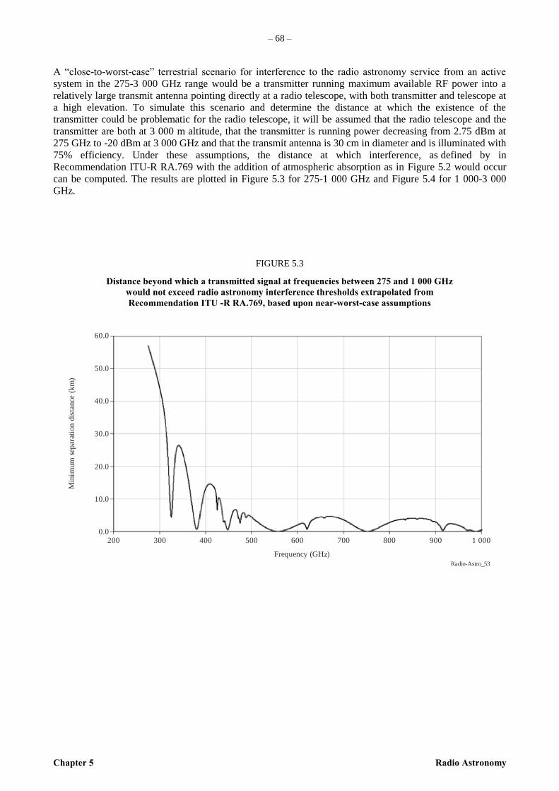
– 68 –
Chapter 5 Radio Astronomy
A “close-to-worst-case” terrestrial scenario for interference to the radio astronomy service from an active
system in the 275-3 000 GHz range would be a transmitter running maximum available RF power into a
relatively large transmit antenna pointing directly at a radio telescope, with both transmitter and telescope at
a high elevation. To simulate this scenario and determine the distance at which the existence of the
transmitter could be problematic for the radio telescope, it will be assumed that the radio telescope and the
transmitter are both at 3 000 m altitude, that the transmitter is running power decreasing from 2.75 dBm at
275 GHz to -20 dBm at 3 000 GHz and that the transmit antenna is 30 cm in diameter and is illuminated with
75% efficiency. Under these assumptions, the distance at which interference, as defined by in
Recommendation ITU-R RA.769 with the addition of atmospheric absorption as in Figure 5.2 would occur
can be computed. The results are plotted in Figure 5.3 for 275-1 000 GHz and Figure 5.4 for 1 000-3 000
GHz.
FIGURE 5.3
Distance beyond which a transmitted signal at frequencies between 275 and 1 000 GHz
would not exceed radio astronomy interference thresholds extrapolated from
Recommendation ITU -R RA.769, based upon near-worst-case assumptions
Radio-Astro_53
2000.0
Frequency (GHz)
Min
imum
sep
arat
ion
dis
tance
(k
m)
300 500 600 700 900 1 000400 800
10.0
20.0
30.0
40.0
50.0
60.0
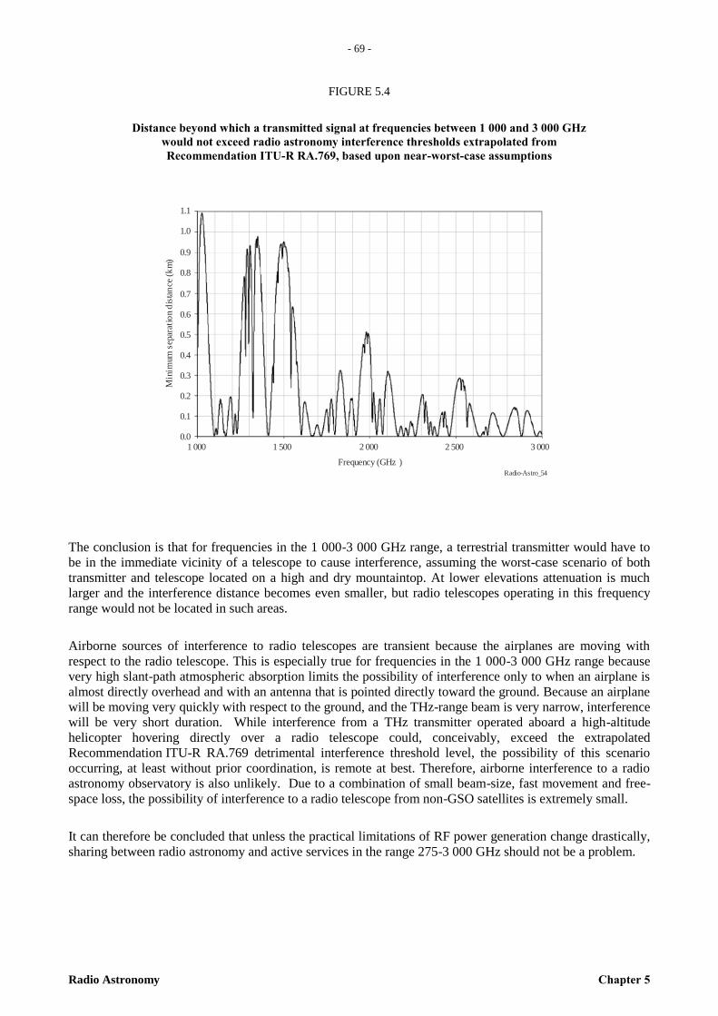
- 69 -
Radio Astronomy Chapter 5
– 6
9 –
FIGURE 5.4
Distance beyond which a transmitted signal at frequencies between 1 000 and 3 000 GHz
would not exceed radio astronomy interference thresholds extrapolated from
Recommendation ITU-R RA.769, based upon near-worst-case assumptions
Radio-Astro_54
1 0000.0
Frequency (GHz )
Min
imum
sep
arat
ion
dis
tan
ce (
km
)
1 500 2 000 2 500 3 000
0.1
0.2
0.3
0.4
0.5
0.6
0.7
0.8
0.9
1.0
1.1
The conclusion is that for frequencies in the 1 000-3 000 GHz range, a terrestrial transmitter would have to
be in the immediate vicinity of a telescope to cause interference, assuming the worst-case scenario of both
transmitter and telescope located on a high and dry mountaintop. At lower elevations attenuation is much
larger and the interference distance becomes even smaller, but radio telescopes operating in this frequency
range would not be located in such areas.
Airborne sources of interference to radio telescopes are transient because the airplanes are moving with
respect to the radio telescope. This is especially true for frequencies in the 1 000-3 000 GHz range because
very high slant-path atmospheric absorption limits the possibility of interference only to when an airplane is
almost directly overhead and with an antenna that is pointed directly toward the ground. Because an airplane
will be moving very quickly with respect to the ground, and the THz-range beam is very narrow, interference
will be very short duration. While interference from a THz transmitter operated aboard a high-altitude
helicopter hovering directly over a radio telescope could, conceivably, exceed the extrapolated
Recommendation ITU-R RA.769 detrimental interference threshold level, the possibility of this scenario
occurring, at least without prior coordination, is remote at best. Therefore, airborne interference to a radio
astronomy observatory is also unlikely. Due to a combination of small beam-size, fast movement and free-
space loss, the possibility of interference to a radio telescope from non-GSO satellites is extremely small.
It can therefore be concluded that unless the practical limitations of RF power generation change drastically,
sharing between radio astronomy and active services in the range 275-3 000 GHz should not be a problem.
– 70 –
Chapter 5 Radio Astronomy
5.8 Sharing with deep-space research
The bands allocated to deep-space research (space-to-Earth) transmissions at 2.3 GHz and 8.4 GHz are
routinely used for VLBI observations for radio astronomy and for geodesy (study of plate tectonics). Deep
space is defined in the RR as the region of space beyond 2 106 km from the Earth. Missions to deep space
involve exploration of planets, comets, asteroids and the solar wind. Typical parameters for space-to-Earth
transmissions from deep-space vehicles are 20 W for the transmitter power and 4 m for the diameter of the
antenna, the latter providing a gain of 36 dBi at 2.3 GHz or 47 dBi at 8.4 GHz. At a distance of 2 106 km
from the Earth the corresponding terrestrial levels of pfd are –148 dB(W/m2) at 2.3 GHz and 137 dB(W/m
2)
at 8.4 GHz. It is clear by reference to Chapter 4 that these levels exceed the harmful thresholds for
interference to total power radio astronomy measurements. However the pfd levels are below the harmful
thresholds for VLBI measurements. Experience to date confirms that, for the particular case of VLBI
measurements, sharing between radio astronomy and deep-space communications is practicable.
For a spacecraft with the same transmitter parameters, a separation distance of 6 107 km would be
necessary to avoid interference harmful to total power radio astronomy measurements. For comparison the
nearest planet Venus has a distance of 4 107 km at its closest approach. Thus in terms of the thresholds in
Chapter 4, signals from spacecraft in the nearer parts of deep space could cause detrimental interference to
radio telescopes sharing the same band, whereas spacecraft on missions to the outer planets would cause very
little interference (and the directions of the interfering spacecraft would be well known). Note that it is here
assumed that the spacecraft signals would be received through side-lobes of the radio telescope which have
gain no greater than 0 dBi.
5.9 Time sharing
Because of the nature of the phenomena observed in radio astronomy, only under special conditions will it be
feasible to devise time-sharing programmes between radio astronomy and active services operating in the
same frequency band. Furthermore users who provide a service to customers may be unwilling or unable to
adopt time sharing. Time sharing may sometimes be possible in principle, but in practice the difficulties
associated with it are operational rather than technical.
Nevertheless, limited time sharing to permit observations at a radio astronomy site may be possible, and may
indeed be necessary on occasion. The special case of receiver blanking to allow observations in the presence
of radar transmitters was already discussed in the previous Chapter. More generally, the science often
requires radio astronomers to observe outside the frequency bands allocated to their service, and in such
cases time sharing with active services may be the only available option. Recommendation ITU-R RA.314
acknowledges this fact, and urges that administrations be asked to provide assistance in the coordination of
experimental observations of spectral lines in bands not allocated to radio astronomy.
5.9.1 Time and frequency sharing coordination
Modern radiotelescopes are capable of observations over an enormous range of frequencies. Telescopes are
often oversubscribed, telescope time is expensive and competition for observing time is fierce.
Consequently, radio astronomers need to operate their telescopes in the most efficient way possible. This
requires that, insofar as possible, they adapt the frequency of observation to the best atmospheric conditions
possible at all times, and some radio astronomy observatories have adopted dynamic scheduling. As an
example, the U.S. National Radio Astronomy Observatory’s Green Bank Telescope (GBT) is capable of
observations in the range 1-100 GHz. Observations at the highest frequencies can however only be made at
certain times in the winter months, under extremely dry atmospheric conditions and it is desirable to exploit
these times to the maximum extent possible. The German Max-Planck Institute’s Bonn radiotelescope covers
a similar frequency range.
Due to the multiplicity of channels used by some of the active services, time coordination, even on short
times scales may, in some cases, be possible. Observatories may relay their schedules to the active services
operating in the bands of interest, and those services may in some cases switch to channels that do not cause
interference to radio astronomy observations. It is recognized that, particularly when radio astronomers
desire to observe outside their allocated bands, such arrangements need to be equitable for all parties, and
need to be implemented on a case-by-case basis. It is to be noted that the effects of propagation vary strongly
with frequency, so that periods of data loss can sometimes be reduced by dynamic rescheduling.
- 71 -
Radio Astronomy Chapter 5
– 7
1 –
REFERENCES
CCIR [1990] Report 696-2 – Feasibility of Frequency Sharing between Radio Astronomy and other Services.
Doc. of the XVIIth Plenary Assembly, Düsseldorf, 1990, Annex to Vol. II, p. 568-584.
GREENHILL, L. J., KNODRATKO, P. T., LOVELL, J. E. J., KUIPER, T. B. H., MORAN, J. M.,
JAUNCEY, D. L. and BAINES, G. P. [2003] Astrophys. J. (Letters), Vol. 582, L11-L14.
– 72 –
Chapter 6 Radio Astronomy
CHAPTER 6
Interference to Radio Astronomy from transmitters in other bands
6.1 Introduction
The cosmic radio emissions that are detected and measured by radio telescopes are far weaker than the
signals used by active (transmitting) services. To measure such weak signals, the receivers used for making
radio astronomical observations are typically the most sensitive that can be achieved with current radio
technology and accessible bandwidth. Because of the weakness of the signals and the sensitivities of the
receivers, radio astronomy observations are extremely vulnerable to interference; this can occur even from
transmitters that do not share the same band. Such interference results from band-edge effects, harmonics of
transmitters, intermodulation effects, etc. The threshold levels of interference to radio astronomy
observations, protection criteria, and limitations to which sharing with other services is feasible, are
discussed in Chapters 4 and 5.
Signal levels encountered in bands adjacent to those used by active services vary widely with the nature of
the service. In addition, designations of services are of a very general nature and any one may involve a
number of different types of transmitting equipment. The highest peak signal levels are likely to be found in
the bands designated for radiolocation and aeronautical radionavigation, since these can include high-
powered radars in aircraft. Mean pfd’s of such signals at relatively isolated observatory sites commonly
exceed –100 dB(W/m2). Very high signal levels are also produced by UHF television.
6.1.1 Definitions from the RR
The following definitions from RR Article 1, Section VI are useful in the discussion of interference from
transmitters in other bands.
Necessary bandwidth (RR No. 1.152): For a given class of emission, the width of the frequency band which
is just sufficient to ensure the transmission of information at the rate and with the quality required under
specified conditions.
Out-of-band emission (RR No. 1.144): Emission on a frequency or frequencies immediately outside the
necessary bandwidth which results from the modulation process, but excluding spurious emissions.
Spurious emission (RR No. 1.145): Emission on a frequency or frequencies which are outside the necessary
bandwidth and the level of which may be reduced without affecting the corresponding transmission of
information. Spurious emissions include harmonic emissions, parasitic emissions, intermodulation products
and frequency conversion products, but exclude out-of-band emissions.
Unwanted emissions (RR No. 1.146): Consist of spurious emissions and out-of-band emissions.
6.1.2 Additional definitions
Some exceptions and modifications to the definitions in § 6.1.1 occur in particular cases. For example,
Recommendation ITU-R SM.1541 contains the following definitions.
Spurious domain11
(of an emission): The frequency range beyond the Out-of-Band (OoB) domain in which
spurious emissions generally predominate.
OoB domain1 (of an emission) the frequency range, immediately outside the necessary bandwidth but
excluding the spurious domain, in which OoB emissions generally predominate.
____________________
11 The terms “OoB domain” and “spurious domain” have been introduced in order to remove some inconsistency now existing
between, on one hand, the definition of the terms “out-of-band emission” and “spurious emission” in RR Article 1 and, on the other
hand, the actual use of these terms in RR Appendix 3 (Rev.WRC-12). OoB and spurious limits apply, respectively, to all unwanted
emissions in the OoB and spurious domains.

- 73 -
Radio Astronomy Chapter 6
– 7
3 –
OoB domain emissions: Any emission outside the necessary bandwidth which occurs in the frequency range
separated from the assigned frequency of the emission by less than 250% of the necessary bandwidth of the
emission will generally be considered an emission in the OoB domain. However, this frequency separation
may be dependent on the type of modulation, the maximum symbol rate in the case of digital modulation, the
type of transmitter, and frequency coordination factors. For example, in the case of some digital, broadband,
or pulse modulated systems, the frequency separation may need to differ from the 250% factor.
Spurious domain emissions: For the purpose of this Recommendation all emissions, including
intermodulation products, conversion products and parasitic emissions, which fall at frequencies separated
from the centre frequency of the emission by 250% or more of the necessary bandwidth of the emission will
generally be considered as emissions in the spurious domain. However, this frequency separation may be
dependent on the type of modulation, the maximum symbol rate in the case of digital modulation, the type of
transmitter, and frequency coordination factors. For example, in the case of some digital, broadband, or
pulse-modulated systems, the frequency separation may need to differ from the 250% factor.
For multichannel or multicarrier transmitters/transponders, where several carriers may be transmitted
simultaneously from a final output amplifier or an active antenna, the centre frequency of the emission is
taken to be the centre of either the assigned bandwidth of the station or of the 3 dB bandwidth of the
transmitter/transponder, using the lesser of the two bandwidths.
OoB spurious emission: The distinction between OoB and spurious emission is usually made in terms of the
frequency, as follows (see Recommendation ITU-R SM.329-9). According to the principles stated in RR
Appendix 3, the spurious domain generally consists of frequencies separated from the centre frequency of
the emission by 250% or more of the necessary bandwidth of the emission. However, this frequency
separation may be dependent on the type of modulation used, the maximum bit rate in the case of digital
modulation, the type of transmitter, and frequency coordination factors. For example, in the case of some
digital, broadband or pulse-modulated systems, the frequency separation may need to differ from the 250%
factor. As the RR forbids any radio service to cause harmful interference outside its allocated band,
transmitter frequencies should be determined so that OoB emissions do not cause harmful interference
outside the allocated band in accordance with RR No. 4.5.
Alternatively, the 250% may apply to channel separation instead of the necessary bandwidth. As an
example, for frequency coordination of the digital fixed service, Recommendation ITU-R F.1191
recommends the use of 250% of the channel separation of the relevant radio-frequency channel
arrangement as frequency boundaries between the OoB and spurious domains.
In case of very narrow or wide bandwidth, this method of determining the spurious domain might not be
appropriate and Recommendation ITU-R SM.1539 provides further guidance.
6.1.3 Mechanisms of interference from transmitters in other bands
Band-edge interference, i.e. interference resulting from a transmitter in an adjacent band, can arise through
three mechanisms:
– Modulation sidebands can fall within the radio astronomy band when the transmitted spectrum from a
transmitter in an adjacent band does not cut off sharply enough at the band edge.
– Two or more strong signals acting upon a non-linear element can generate beat frequencies of the form
(mf1 nf2), where f1 and f2 are transmitted frequencies, and m and n are integers. The integer (m n) is
called the order of the intermodulation. The non-linear element may be in the output of a transmitter,
the input stages of the radio astronomy receiver, or a nearby object such as a rusty joint in a tower or
fence in an area where the electric fields are strong.
– The radio astronomy receiver may respond to signals in an adjacent band if the sensitivity of the
receiver to frequencies outside the radio astronomy band is not sufficiently low.
Interference from transmitters in bands more widely separated in frequency from a radio astronomy band can
result from the following mechanisms.
– Harmonics of the allocated transmitter frequency are likely to be generated in the transmitter, and may
be radiated at a level that can cause interference to radio astronomical observations.
– 74 –
Chapter 6 Radio Astronomy
– Intermodulation between two signals that are rather widely separated in frequency can generate a third
frequency that is well separated from either of the first two.
– The use of wideband modulation and spread spectrum techniques can result in very extensive spectral
sidebands which, if not filtered at the transmitter output, can cause serious interference.
Intermodulation in the input stages of the receiver and insufficient rejection of signals outside the edges of
the radio astronomy band both result from inadequate receiver design. Radio astronomy receivers should
contain sufficient filtering at the input stages to reject signals that may cause intermodulation. Also, they
should be designed with IF filters capable of providing the required rejection at the edges of the radio
astronomy band, which may be as much as –100 dB relative to the band centre.
In general, allocating bands adjacent to radio astronomy bands to services using high-powered transmitters
may lead to difficult and expensive technical problems. Some of the mechanisms of interaction, such as
those involving harmonics or modulation sidebands, depend strongly upon the characteristics of the
transmitter and must be examined individually for different services. Transmissions from satellites and
aircraft are a particular problem for radio astronomy because LoS propagation conditions commonly exist.
Services such as the radiodetermination satellite service and the digital communications services, that use
broadband modulation and spread spectrum techniques from satellites, are examples that have been found to
be particularly troublesome to radio astronomy.
6.2 Limits for unwanted emissions from active services
6.2.1 Limits within the spurious emissions domain
Limits on spurious emissions are given in RR Appendix 3 and also in Recommendation ITU-R SM.329
(Spectrum management series), which specifies various categories. These include:
– Category A limits are the attenuation values used to calculate maximum permitted spurious domain
emission power levels. RR Appendix 3 is derived from Category A limits;
– Category B limits are an example of more stringent spurious limits than Category A limits. They are
based on limits defined and adopted in Europe and used by some other countries;
– Category C limits are an example of more stringent spurious limits than Category A limits. They are
based on limits defined and adopted in the United States of America and Canada and used by some
other countries.
– Category D limits are an example of more stringent spurious limits than Category A limits. They are
based on limits defined and adopted in Japan and used by some other countries.
– Category Z: Radiation limits for ITE specified by the International Special Committee on Radio
Interference (CISPR).
Limits are given in terms of the maximum power level of the spurious emission expressed as dBs below the
power into the antenna transmission line.
For terrestrial services, the Category A limits, with which radio astronomers are most concerned, specify a
minimum attenuation of 43 10 log P dBc, or 70 dBc, whichever is less stringent, where P is the mean
power into the transmission line. The spurious emission for this case is measured in a reference bandwidth of
100 kHz for frequencies of 30 MHz to 1 GHz, and 1 MHz for frequencies above 1 GHz.
For space services, the Category A limits specify 43 10 log P dBc, or 60 dBc, whichever is less stringent.
However, for space services the reference bandwidth in which the spurious emission is measured is specified
as 4 kHz, thus resulting in a power spectral density that is less stringent than for terrestrial services by 14 dB
(10 log(4/100) dB) for 30 MHz to 1 GHz, and 24 dB (10 log(4/1 000) dB) for frequencies above 1 GHz.
As an example of the effects of spurious emissions from space services, a satellite at a distance h m
above a radio astronomy station may produce a spurious spfd of 79 10 log (4h2) GSAT dB(W(m
–2 Hz
1),
where GSAT is the gain of the satellite antenna in the direction of the radio observatory at the frequency of the
spurious emission. To estimate values of the spurious spfd for the frequencies in the radio astronomy bands
for a geostationary-orbit satellite we use h 6.39 106 m and arbitrarily take values of GSAT corresponding to
a 1 m2 aperture for the satellite antenna. We allow a maximum gain of 40 dB for which the footprint
diameter is 1 400 km. The resulting values of spfd are shown by the dotted curve in Figure 6.1. Next, as an
- 75 -
Radio Astronomy Chapter 6
– 7
5 –
example of a low-Earth orbit (LEO) satellite we take h 800 km, and GSAT again corresponding to a 1 m2
aperture, with a maximum value of 20 dB for which the footprint diameter is about 300 km, which is about
as small a footprint as might commonly be used. The resulting values are plotted as the solid curve in Figure
6.1, in which the threshold values of interference for radio astronomy continuum observations, as given in
Recommendation ITU-R RA.769, are shown as crosses. The spurious spfd curves in Figure 6.2 show worst-
case values since we have assumed that the full gain of the satellite antenna occurs in the direction of the
radio astronomy station. Also, for simplicity we have used distances for a satellite at the zenith and ignored
atmospheric attenuation and similar small effects. However, the extent to which the permitted levels of spfd
exceed the detrimental thresholds, i.e. 20 to 50 dB, clearly indicates that in general the spurious emission
limits fall well short of protecting radio astronomy. For terrestrial services the limits on spurious spfd above
1 GHz frequency are 24 dB more stringent than for space services, because of the different reference
bandwidths. Distances of terrestrial transmitters are usually less than those of transmitters for space services,
but terrain shielding can provide substantial protection. For LoS transmissions, the spurious emission limits
again fail to protect radio astronomy in most cases. Recommendation ITU-R SM.329, which specifies the
limits on spurious emissions, also lists the radio astronomy interference thresholds (in Annex 3 of the
Recommendation), but protection to these limits is not mandated, and is regarded as something to be
considered for individual cases as new systems arise.
6.2.2 Limits within the OoB emissions domain
Limits on OoB emissions are given in Recommendation ITU-R SM.1541. Briefly, this Recommendation
gives emission masks for many services, which show limits in the region from the edges of the necessary
band to the inner edges of the region of spurious emissions. These limits are less stringent than those for
spurious emission, but fall off towards the spurious limits at the OoB/spurious boundaries. Thus again the
limits are not intended to protect radio astronomy, and coordination is left to be considered on a case-by-case
basis.
6.2.3 Limits on unwanted emissions of active services to protect radio astronomy bands
A number of footnotes within the RR are intended to protect the radio astronomy service from unwanted
emissions of active services (see for example RR No. 5.208A). At many WRCs, additional footnotes have
been developed in order to provide additional protection to the radio astronomy service from existing and
new active services.
Footnote RR 5.443B concerns protection from unwanted emissions of the radionavigation-satellite service
(space-to-Earth) operating in the band 5 010-5 030 MHz:
“5.443B … In order not to cause harmful interference to the microwave landing system operating above
5 030 MHz, the aggregate power flux-density produced at the Earth’s surface in the band 5 030-5 150 MHz
by all the space stations within any radionavigation-satellite service system (space-to-Earth) operating in the
band 5 010-5 030 MHz shall not exceed −124.5 dB(W/m2) in a 150 kHz band. In order not to cause harmful
interference to the radio astronomy service in the band 4 990-5 000 MHz, radionavigation-satellite service
systems operating in the band 5 010-5 030 MHz shall comply with the limits in the band 4 990-5 000 MHz
defined in Resolution 741 (Rev.WRC-12). (WRC-12)”
Footnotes RR 5.511A and 5.511F concern protection from unwanted emissions of the MSS (space-to-Earth)
operating in the 15.43-15.63 GHz:
“5.511A … In order to protect the radio astronomy service in the band 15.35-15.4 GHz, the aggregate
power flux-density radiated in the 15.35-15.4 GHz band by all the space stations within any feeder-link of a
non-geostationary system in the mobile-satellite service (space-to-Earth) operating in the 15.43-15.63 GHz
band shall not exceed the level of –156 dB(W/m2) in a 50 MHz bandwidth, into any radio astronomy
observatory site for more than 2% of the time. (WRC-2000)”

– 76 –
Chapter 6 Radio Astronomy
FIGURE 6.1
spfd at the ground corresponding to spurious
emission limits for satellites
Radio-Astro_61
0.1
Frequency (GHz)
spfd
at
gro
und
(dB
(W/(
m ·
Hz))
)2
The solid curve and the dotted curve show possible values of spfd at the ground level from LEO and
geostationary orbit satellites, respectively, radiating at the limit for spurious emissions for spacecraft. See text
for details. The crosses show the threshold values for detrimental interferences to radio astronomy as given
in Table 4.1.
–180
–200
–220
–240
–260
1 10 103
102
6.3 Performance of radio astronomy receivers
6.3.1 Filtering of band-edge interference
To calculate the effective input power P received in a radio astronomy receiver from adjacent band signals,
the band-edge response of the receiver has to be known with some accuracy. For example, consider the
upper-frequency edge of the band in Figure 6.2, in which –a0 dB is the level by which the relative gain of the
radiometer has been reduced at the band edge and –k dB/MHz is the slope of the receiver response at that
point.
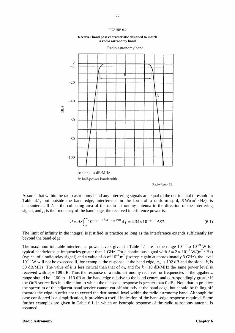
- 77 -
Radio Astronomy Chapter 6
– 7
7 –
FIGURE 6.2
Receiver band pass characteristic designed to match
a radio astronomy band
Radio-Astro_62
(dB
)
Radio astronomy band
A k: slope – dB/MHz
B: half-power bandwidth
–20
–60
–40
–80
–100
0–3
A
B
Assume that within the radio astronomy band any interfering signals are equal to the detrimental threshold in
Table 4.1, but outside the band edge, interference in the form of a uniform spfd, S W/(m2 · Hz), is
encountered. If A is the collecting area of the radio astronomy antenna in the direction of the interfering
signal, and f0 is the frequency of the band edge, the received interference power is:
kASfASPa
f
ffka/1034.4d10
10/–10/)–(10[– 0
0
06–
0
(6.1)
The limit of infinity in the integral is justified in practice so long as the interference extends sufficiently far
beyond the band edge.
The maximum tolerable interference power levels given in Table 4.1 are in the range 10–17
to 1021
W for
typical bandwidths at frequencies greater than 1 GHz. For a continuous signal with S 2 10–13
W/(m2 · Hz)
(typical of a radio relay signal) and a value of A of 10–3
m2 (isotropic gain at approximately 3 GHz), the level
10–21
W will not be exceeded if, for example, the response at the band edge, a0, is 102 dB and the slope, k, is
50 dB/MHz. The value of k is less critical than that of a0, and for k 10 dB/MHz the same power level is
received with a0 109 dB. Thus the response of a radio astronomy receiver for frequencies in the gigahertz
range should be 100 to 110 dB at the band edge relative to the band centre, and correspondingly greater if
the OoB source lies in a direction in which the telescope response is greater than 0 dBi. Note that in practice
the spectrum of the adjacent-band service cannot cut off abruptly at the band edge, but should be falling off
towards the edge in order not to exceed the detrimental level within the radio astronomy band. Although the
case considered is a simplification, it provides a useful indication of the band-edge response required. Some
further examples are given in Table 6.1, in which an isotropic response of the radio astronomy antenna is
assumed.
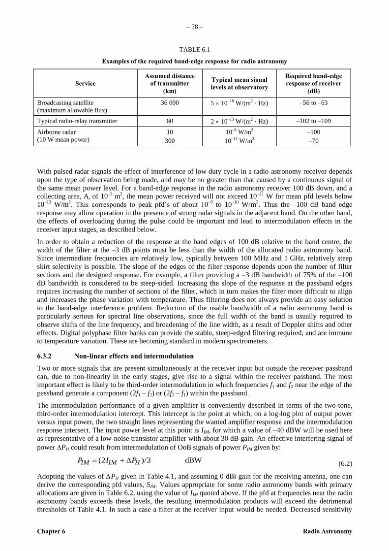
– 78 –
Chapter 6 Radio Astronomy
TABLE 6.1
Examples of the required band-edge response for radio astronomy
With pulsed radar signals the effect of interference of low duty cycle in a radio astronomy receiver depends
upon the type of observation being made, and may be no greater than that caused by a continuous signal of
the same mean power level. For a band-edge response in the radio astronomy receiver 100 dB down, and a
collecting area, A, of 10–3
m2, the mean power received will not exceed 10
–21 W for mean pfd levels below
10–13
W/m2. This corresponds to peak pfd’s of about 10
–9 to 10
–10 W/m
2. Thus the –100 dB band edge
response may allow operation in the presence of strong radar signals in the adjacent band. On the other hand,
the effects of overloading during the pulse could be important and lead to intermodulation effects in the
receiver input stages, as described below.
In order to obtain a reduction of the response at the band edges of 100 dB relative to the band centre, the
width of the filter at the –3 dB points must be less than the width of the allocated radio astronomy band.
Since intermediate frequencies are relatively low, typically between 100 MHz and 1 GHz, relatively steep
skirt selectivity is possible. The slope of the edges of the filter response depends upon the number of filter
sections and the designed response. For example, a filter providing a –3 dB bandwidth of 75% of the –100
dB bandwidth is considered to be steep-sided. Increasing the slope of the response at the passband edges
requires increasing the number of sections of the filter, which in turn makes the filter more difficult to align
and increases the phase variation with temperature. Thus filtering does not always provide an easy solution
to the band-edge interference problem. Reduction of the usable bandwidth of a radio astronomy band is
particularly serious for spectral line observations, since the full width of the band is usually required to
observe shifts of the line frequency, and broadening of the line width, as a result of Doppler shifts and other
effects. Digital polyphase filter banks can provide the stable, steep-edged filtering required, and are immune
to temperature variation. These are becoming standard in modern spectrometers.
6.3.2 Non-linear effects and intermodulation
Two or more signals that are present simultaneously at the receiver input but outside the receiver passband
can, due to non-linearity in the early stages, give rise to a signal within the receiver passband. The most
important effect is likely to be third-order intermodulation in which frequencies f1 and f2 near the edge of the
passband generate a component (2f1 – f2) or (2f2 – f1) within the passband.
The intermodulation performance of a given amplifier is conveniently described in terms of the two-tone,
third-order intermodulation intercept. This intercept is the point at which, on a log-log plot of output power
versus input power, the two straight lines representing the wanted amplifier response and the intermodulation
response intersect. The input power level at this point is IIM, for which a value of –40 dBW will be used here
as representative of a low-noise transistor amplifier with about 30 dB gain. An effective interfering signal of
power PH could result from intermodulation of OoB signals of power PIM given by:
dBW3/)2( HMIMI PIP (6.2)
Adopting the values of PH given in Table 4.1, and assuming 0 dBi gain for the receiving antenna, one can
derive the corresponding pfd values, SIM. Values appropriate for some radio astronomy bands with primary
allocations are given in Table 6.2, using the value of IIM quoted above. If the pfd at frequencies near the radio
astronomy bands exceeds these levels, the resulting intermodulation products will exceed the detrimental
thresholds of Table 4.1. In such a case a filter at the receiver input would be needed. Decreased sensitivity
Service
Assumed distance
of transmitter
(km)
Typical mean signal
levels at observatory
Required band-edge
response of receiver
(dB)
Broadcasting satellite
(maximum allowable flux)
36 000 5 10–18
W/(m2 · Hz) –56 to –63
Typical radio-relay transmitter 60 2 10–13
W/(m2 · Hz) –102 to –109
Airborne radar
(10 W mean power)
10
300
10–8
W/m2
10–11
W/m2
–100
–70
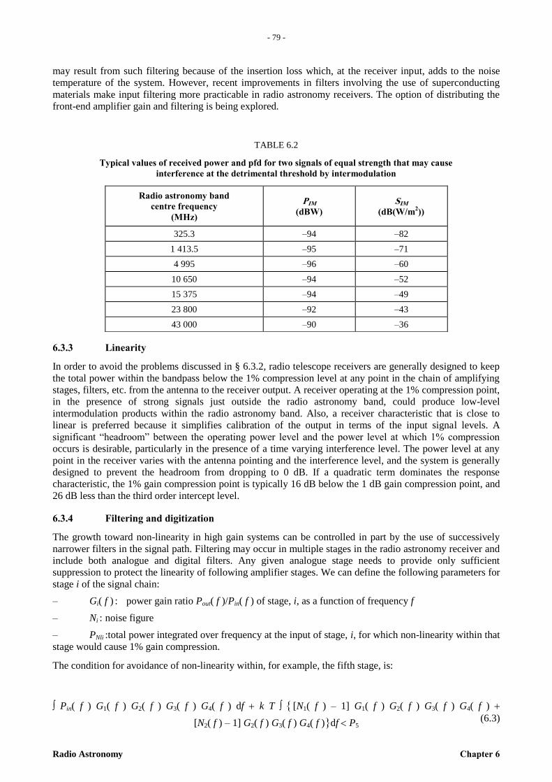
- 79 -
Radio Astronomy Chapter 6
– 7
9 –
may result from such filtering because of the insertion loss which, at the receiver input, adds to the noise
temperature of the system. However, recent improvements in filters involving the use of superconducting
materials make input filtering more practicable in radio astronomy receivers. The option of distributing the
front-end amplifier gain and filtering is being explored.
TABLE 6.2
Typical values of received power and pfd for two signals of equal strength that may cause
interference at the detrimental threshold by intermodulation
6.3.3 Linearity
In order to avoid the problems discussed in § 6.3.2, radio telescope receivers are generally designed to keep
the total power within the bandpass below the 1% compression level at any point in the chain of amplifying
stages, filters, etc. from the antenna to the receiver output. A receiver operating at the 1% compression point,
in the presence of strong signals just outside the radio astronomy band, could produce low-level
intermodulation products within the radio astronomy band. Also, a receiver characteristic that is close to
linear is preferred because it simplifies calibration of the output in terms of the input signal levels. A
significant “headroom” between the operating power level and the power level at which 1% compression
occurs is desirable, particularly in the presence of a time varying interference level. The power level at any
point in the receiver varies with the antenna pointing and the interference level, and the system is generally
designed to prevent the headroom from dropping to 0 dB. If a quadratic term dominates the response
characteristic, the 1% gain compression point is typically 16 dB below the 1 dB gain compression point, and
26 dB less than the third order intercept level.
6.3.4 Filtering and digitization
The growth toward non-linearity in high gain systems can be controlled in part by the use of successively
narrower filters in the signal path. Filtering may occur in multiple stages in the radio astronomy receiver and
include both analogue and digital filters. Any given analogue stage needs to provide only sufficient
suppression to protect the linearity of following amplifier stages. We can define the following parameters for
stage i of the signal chain:
– Gi( f ) : power gain ratio Pout( f )/Pin( f ) of stage, i, as a function of frequency f
– Ni : noise figure
– PNli :total power integrated over frequency at the input of stage, i, for which non-linearity within that
stage would cause 1% gain compression.
The condition for avoidance of non-linearity within, for example, the fifth stage, is:
Pin( f ) G1( f ) G2( f ) G3( f ) G4( f ) df k T [N1( f ) – 1] G1( f ) G2( f ) G3( f ) G4( f )
[N2( f ) – 1] G2( f ) G3( f ) G4( f )df P5 (6.3)
Radio astronomy band
centre frequency
(MHz)
PIM
(dBW) SIM
(dB(W/m2))
325.3 –94 –82
1 413.5 –95 –71
4 995 –96 –60
10 650 –94 –52
15 375 –94 –49
23 800 –92 –43
43 000 –90 –36
– 80 –
Chapter 6 Radio Astronomy
where Pin( f ) is the input power from the antenna, k is Boltzmann’s constant, T 290 K, and it has been
assumed that the gain in the first two stages is sufficiently large that the noise contribution of later stages can
be ignored.
In most radio astronomy receivers used with a single antenna, the signals are processed in an autocorrelator
to provide total-power spectra. In the case of an array of antennas the signals are processed by a cross-
correlator system. In either case the IF signal is digitized and the subsequent processing is done digitally. An
anti-aliasing analogue filter is required at the input of the analogue-to-digital (A/D) converter, to establish
frequency cut-offs of the IF spectrum, so that sampling can be performed at twice the signal bandwidth as
required for Nyquist sampling. If non-linearity is avoided in the analogue system and aliasing is avoided in
the A/D conversion, then further filtering can be inserted digitally before the autocorrelator or cross-
correlator stages. Interfering signals at the detrimental thresholds given in Recommendation ITU-R RA.769,
(and Tables 4.1 and 4.2) result in signal levels in the IF system that are some 40 to 80 dB below that at which
there is danger of non-linearity. Thus signals that exceed these levels by some tens of decibels can be
adequately rejected by the digital filters if they lie outside the radio astronomy band. Digital filters of
finite-impulse-response (FIR) type can provide very sharp cutoff at the band edges, and together with the
analogue filters in the earlier stages can result in rejection in excess of 100 dB. Polyphase filters, in which
the IF signal is convolved with a digital approximation of a sinc function, are particularly effective and are
coming into general use. Thus it is generally possible to design radio astronomy receivers to reject
interference that falls outside the radio astronomy band.
6.4 Interference from transmitters of services in other bands
Recommendations ITU-R RA.517 – Protection of the radio astronomy services from transmitters operating
in adjacent bands, and ITU-R RA.611 – Protection of the radio astronomy service from spurious emissions,
list some of the cases where transmitters operating in adjacent or non adjacent bands may cause interference
to radio astronomy.
6.4.1 Services which could cause interference to radio astronomy through adjacent-band and
harmonic mechanisms
Most active services operating in bands adjacent to radio astronomy bands, or at frequencies that are sub-
harmonics of radio astronomy frequencies, are potential sources of interference to radio astronomy.
However, the likelihood of any service causing such interference depends strongly upon the nature of the
transmissions. For example, transmissions by the fixed and mobile services (except aeronautical mobile)
have rarely presented problems. Services most likely to cause interference through intermodulation and
harmonic effects include those with high output power, such as UHF television. Also, services using
transmissions from satellites can cause serious problems because of LoS propagation, and the need to
minimise weight in a satellite, which can make the installation of filters difficult and expensive. Techniques
that produce a wide spectrum of sidebands, such as direct sequence spread-spectrum, without adequate
filtering of the unused sidebands, have the potential to cause very serious problems to radio astronomy.
6.4.2 The transition to digital television and its impact on the unprotected use by the radio
astronomy service of bands used for terrestrial television broadcasting
Television has become a fundamental form of communication in every region of the world. Its utility as a
source of news, entertainment and emergency information has been evident since its inception more than 60
years ago. Presently providing coverage to a global population numbering in the billions, terrestrial
television broadcasting is one of the most ubiquitous uses of the radio spectrum.
The radio astronomy service does not share any allocations with terrestrial television broadcasting; however,
such broadcasts generally occupy spectrum that is extremely important to low-frequency astrophysics and
the observation of red shifted neutral hydrogen (HI) arising from early epochs in the formation of the
universe. To date, radio astronomers have made use of TV bands to conduct observations, in accordance with
No. 4.4 of the Radio Regulations (RR).
At the present time, many countries are transitioning from analogue to digital television broadcast standards
and some are also revising their broadcast allocations to recover spectrum that is expected to be freed up by
the so-called “digital dividend”. Some aspects of the digital transition are expected to result in a reduction in
the ability of radio astronomers to make use of the terrestrial television broadcast bands for observations that

- 81 -
Radio Astronomy Chapter 6
– 8
1 –
are currently conducted on an unprotected basis (see Figure 6.3). Some aspects may improve the ability to
make passive observations in the TV bands.
The sections below summarize the plans for the transition to digital television for several countries around
the world with current radio astronomy programmes operating within bands used for terrestrial television
broadcasting, and for countries of strategic importance to future radio astronomy stations presently under
design and development that intend to utilize such bands. The impact of service rules for digital television on
the use of the television broadcast bands for radio astronomy is discussed.
FIGURE 6.3
An example of the impact of digital TV signals compared to analogue TV. The spectra were obtained
at a radio astronomy site during a brief period of highly enhanced propagation.
The TV signals are originating from approximately 290 km away
Radio-Astro_63
The digital signal from 181-188 MHz “fills” the spectrum much more substantially than the analogue TV
signals occupying 174-181, 188-195, and 195-202 MHz, whose spectra are concentrated in discrete video,
chrominance, and audio carriers
6.4.2.1 Australia
The Australian Government has announced a programme to switchover from analogue to digital
transmissions. Digital television has been planned for operation within existing allocated broadcasting
services bands in bands III (174-230 MHz), IV (526-582 MHz) and V (582-820 MHz). Australian terrestrial
television broadcasting services have been planned on a 7 MHz channel raster in both VHF and UHF bands.
Australia’s digital services are typically planned with a maximum e.r.p. of 6 dB less than same band
analogue television services.
There are no Australian allocations to radio astronomy in these bands and therefore radio telescopes are sited
in less populated areas to minimize the risk of interference from various radiocommunication systems
including broadcasting. The Parkes radio telescope currently observes in the band 700-764 MHz on a no
protection from interference basis. The Australian Square Kilometre Array (SKA) Pathfinder (ASKAP)
telescope, planned for operation from 2013, will have an operating frequency range of 700 to 1 800 MHz.
Furthermore, Australia is a potential site for the SKA.
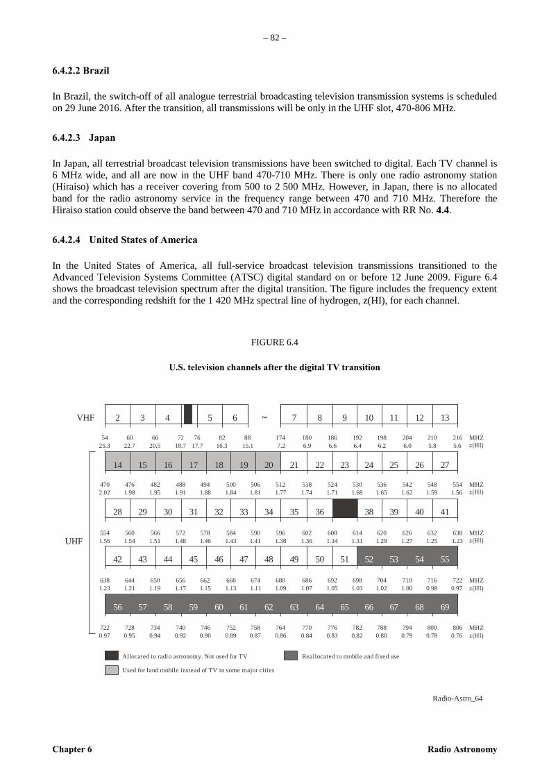
– 82 –
Chapter 6 Radio Astronomy
6.4.2.2 Brazil
In Brazil, the switch-off of all analogue terrestrial broadcasting television transmission systems is scheduled
on 29 June 2016. After the transition, all transmissions will be only in the UHF slot, 470-806 MHz.
6.4.2.3 Japan
In Japan, all terrestrial broadcast television transmissions have been switched to digital. Each TV channel is
6 MHz wide, and all are now in the UHF band 470-710 MHz. There is only one radio astronomy station
(Hiraiso) which has a receiver covering from 500 to 2 500 MHz. However, in Japan, there is no allocated
band for the radio astronomy service in the frequency range between 470 and 710 MHz. Therefore the
Hiraiso station could observe the band between 470 and 710 MHz in accordance with RR No. 4.4.
6.4.2.4 United States of America
In the United States of America, all full-service broadcast television transmissions transitioned to the
Advanced Television Systems Committee (ATSC) digital standard on or before 12 June 2009. Figure 6.4
shows the broadcast television spectrum after the digital transition. The figure includes the frequency extent
and the corresponding redshift for the 1 420 MHz spectral line of hydrogen, z(HI), for each channel.
FIGURE 6.4
U.S. television channels after the digital TV transition
Radio-Astro_64
2 3 4 5 6 7 8 9 10 11 12 13
14 21 22 23 24 25 26 2715 16 17 18 19 20
28
42
56
35
49
63
36
50
64
51
65
38
52
66
39
53
67
40
54
68
41
55
69
29
43
57
30
44
58
31
45
59
32
46
60
33
47
61
34
48
62
54 60 66 72 76 82 88 174 180 186 192 198 204 210 216
25.3 22.7 20.5 18.7 17.7 16.3 15.1 7.2 6.9 6.6 6.4 6.2 6.0 5.8 5.6
VHF
470 476 482 488 494 500 506 512 518 524 530 536 542 548 554
2.02 1.98 1.95 1.91 1.88 1.84 1.81 1.77 1.74 1.71 1.68 1.65 1.62 1.59 1.56
554 560 566 572 578 584 590 596 602 608 614 620 626 632 638
1.56 1.54 1.51 1.48 1.46 1.43 1.41 1.38 1.36 1.34 1.31 1.29 1.27 1.25 1.23
638 644 650 656 662 668 674 680 686 692 698 704 710 716 722
1.23 1.21 1.19 1.17 1.15 1.13 1.11 1.09 1.07 1.05 1.03 1.02 1.00 0.98 0.97
722 728 734 740 752 758 764 770 776 782 788 794 800 806
0.97 0.95 0.94 0.92 0.90 0.89 0.87 0.86 0.84 0.83 0.82 0.80 0.79 0.78 0.76
746
UHF
Allocated to radio astronomy. Not used for TV
Used for land mobile instead of TV in some major cities
Reallocated to mobile and fixed use
~
MHZ
z(HI)
MHZ
z(HI)
MHZ
z(HI)
MHZ
z(HI)
MHZ
z(HI)
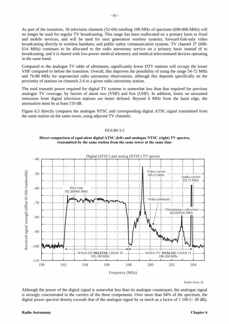
- 83 -
Radio Astronomy Chapter 6
– 8
3 –
As part of the transition, 18 television channels (52-69) totalling 108 MHz of spectrum (698-806 MHz) will
no longer be used for regular TV broadcasting. This range has been reallocated on a primary basis to fixed
and mobile services, and will be used for next generation wireless systems; forward-link-only video
broadcasting directly to wireless handsets; and public safety communication systems. TV channel 37 (608-
614 MHz) continues to be allocated to the radio astronomy service on a primary basis instead of to
broadcasting, and it is shared with low-power medical telemetry and medical telecommand devices operating
in the same band.
Compared to the analogue TV table of allotments, significantly fewer DTV stations will occupy the lower
VHF compared to before the transition. Overall, this improves the possibility of using the range 54-72 MHz
and 76-88 MHz for unprotected radio astronomy observations, although this depends specifically on the
proximity of stations on channels 2-6 to a given radio astronomy station.
The total transmit power required for digital TV systems is somewhat less than that required for previous
analogue TV coverage, by factors of about two (VHF) and five (UHF). In addition, limits on unwanted
emissions from digital television stations are better defined. Beyond 6 MHz from the band edge, the
attenuation must be at least 110 dB.
Figure 6.5 directly compares the analogue NTSC and corresponding digital ATSC signal transmitted from
the same station on the same tower, using adjacent TV channels.
FIGURE 6.5
Direct comparison of equivalent digital ATSC (left) and analogue NTSC (right) TV spectra,
transmitted by the same station from the same tower at the same time
Radio-Astro_65
Frequency (MHz)
198190–110
192 194 196 200 202 204
–100
–90
–80
–70
–60
–50
–40
Rec
eiv
ed s
ignal
stre
ngth
(d
Bm
/10
kH
z b
and
wid
th)
Pilot tone192.309441 MHz
Video carrier199.25 MHz
Audio carrier203.75 MHz
Video sideband
Chrominance subcarrier202.829545 MHz
WXIA-DT CHAN 10192-198 MHz
DIGITAL WXIA-TV CHAN 11198-204 MHz
ANALOG
Digital (ATSC) and analog (NTSC) TV spectra
Although the power of the digital signal is somewhat less than its analogue counterpart, the analogue signal
is strongly concentrated in the carriers of the three components. Over more than 94% of the spectrum, the
digital power spectral density exceeds that of the analogue signal by as much as a factor of 1 100 (> 30 dB).
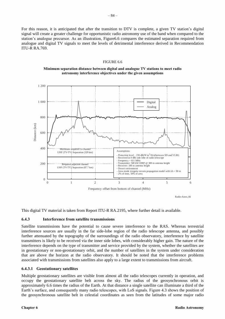
– 84 –
Chapter 6 Radio Astronomy
For this reason, it is anticipated that after the transition to DTV is complete, a given TV station’s digital
signal will create a greater challenge for opportunistic radio astronomy use of the band when compared to the
station’s analogue precursor. As an illustration, Figure6.6 compares the estimated separation required from
analogue and digital TV signals to meet the levels of detrimental interference derived in Recommendation
ITU-R RA.769.
FIGURE 6.6
Minimum separation distance between digital and analogue TV stations to meet radio
astronomy interference objectives under the given assumptions
Radio-Astro_66
Frequency offset from bottom of channel (MHz)
0 1 2 3 4 5 60
200
400
600
800
1 000
1 200
Dis
tance
(km
)
Maximum required co-channel
UHF (TV-TV) Separation (329 km)
Required adjacent channel
UHF (TV-TV) Separation (87.7 km)
Digital
Analog
Assumptions:
- Protection level: –230 dB(W/m /Hz)(between SD and VLBI)- Received in 0 dBi side lobe of radio telescope- Frequency = 611 MHz- Transmitter: 500 kW EIRP @ 300 m antenna height- Receiver: 100 m antenna height- Desert environment- Area-mode irregular terrain propagation model with h = 90 m- 2% of time, 50% of area
2
This digital TV material is taken from Report ITU-R RA.2195, where further detail is available.
6.4.3 Interference from satellite transmissions
Satellite transmissions have the potential to cause severe interference to the RAS. Whereas terrestrial
interference sources are usually in the far side-lobe region of the radio telescope antenna, and possibly
further attenuated by the topography of the surroundings of the radio observatory, interference by satellite
transmitters is likely to be received via the inner side lobes, with considerably higher gain. The nature of the
interference depends on the type of transmitter and service provided by the system, whether the satellites are
in geostationary or non-geostationary orbit, and the number of satellites in the system under consideration
that are above the horizon at the radio observatory. It should be noted that the interference problems
associated with transmissions from satellites also apply to a large extent to transmissions from aircraft.
6.4.3.1 Geostationary satellites
Multiple geostationary satellites are visible from almost all the radio telescopes currently in operation, and
occupy the geostationary satellite belt across the sky. The radius of the geosynchronous orbit is
approximately 6.6 times the radius of the Earth. At that distance a single satellite can illuminate a third of the
Earth’s surface, and consequently many radio telescopes, with LoS signals. Figure 4.3 shows the position of
the geosynchronous satellite belt in celestial coordinates as seen from the latitudes of some major radio

- 85 -
Radio Astronomy Chapter 6
– 8
5 –
astronomy observatories. Plans for the development of some active services call for a large number of
geostationary satellites. Such a series of potential sources of interference that may be received through the
near side-lobes of the radio telescope antenna pattern could present a unique interference problem to radio
astronomers.
Detrimental thresholds for interference to radio astronomy are given in Recommendation ITU-R RA.769.
Listed there is the level, in each radio astronomy band, of the power entering the receiver that is just
sufficient to cause detrimental interference. Also listed are the pfd’s (dB(W/m2)) causing detrimental
interference, which are calculated with the assumption that the gain of the radio telescope is 0 dBi in the
direction of the interfering source. Such a gain is appropriate for consideration of terrestrial sources of
interference confined to the neighbourhood of the horizon. For the case of geostationary sources, the
situation is different.
If we assume that the radio astronomy antenna has the side-lobe characteristics assumed in Recommendation
ITU-R SA.509, the side-lobe gain falls to 0 dBi at 19 from the axis of the main beam. For such an antenna
the detrimental interference level will be exceeded if the main beam is pointed within 19 of a satellite that
produces within the radio astronomy bandwidth a pfd at the radio observatory equal to the detrimental
threshold in Recommendation ITU-R RA.769. A series of satellites spaced at intervals of about 30 along the
geostationary-satellite orbit radiating interference at this level would result in a zone of width approximately
38 centred on the orbit in which radio astronomy observation free from detrimental interference would be
precluded. The width of this precluded zone would increase with the number of interfering satellites in the
orbit, and could, in principle, cover the whole sky. The effective number of interfering satellites will depend
upon whether the interfering signals are beamed by the satellites’ transmitting antennas or are more widely
radiated. An OoB emission that is not widely separated from the satellite’s transmitter frequency is likely to
be directed by the antennas in a way similar to that of the intended signals. Unwanted emissions that are
more widely separated in frequency, such as harmonics, may be radiated more widely but should be more
easily removed by filtering at the transmitter.
A solution to the problem of interference from geostationary satellites clearly involves a compromise
between the area of sky lost to radio astronomy observations and the difficulty of suppressing unwanted
emissions from the satellite transmitters. Examination of Figure 4.3 shows that the position of the
geostationary orbit in the sky, as seen from the Earth, changes by approximately 10 as one goes from
observatories in one hemisphere to those in the other. Thus if observations can be made to within 5 of the
geostationary orbit, each position in the sky can be observed from at least one existing observatory, provided
that it is suitably equipped for the particular observation. The desirability of reducing spurious emissions to
allow radio astronomy observations within 5 of the geostationary orbit is discussed in Chapter 4.
This discussion of radiation from geostationary satellites is based on the assumption that the orbits are
located in the equatorial plane of the Earth. However, for purposes of frequency coordination, a definition of
geostationary satellites includes all geosynchronous satellites with inclination angles less than 15. The effect
of the orbital inclination upon considerations of frequency coordination for radio astronomy will depend
upon the distribution of inclination angles of those satellites that are potential sources of interference.
6.4.3.2 Non-geostationary satellites
The potential for detrimental interference from non-geostationary LEOs is exacerbated by their operation in
large numbers, which make it possible for many of them to be simultaneously above the horizon at a radio
observatory, and within LoS of the radio telescope antenna. This leads to a situation where the radio
telescope antenna can receive unwanted emissions from those visible non-geostationary LEOs through near
and far side-lobes of the antenna beam, and also through the main beam. The interference problem is
complicated by the continually changing directions of arrival of the interfering signals, and the need for the
radio telescope antenna to track the celestial source under observation. Multiple inputs of strong signals may
drive the operating point of the receiver into a non-linear region, resulting in the generation of
intermodulation products.
The impact of unwanted emissions produced at radio astronomy sites by a constellation of satellites in (low)
non-geostationary orbits may be determined using the epfd methodology described in Recommendation ITU-
R S.1586 – Calculation of unwanted emission levels produced by a non-geostationary fixed-satellite service
satellite system at radio astronomy sites, or Recommendation ITU-R M.1583 – Interference calculations
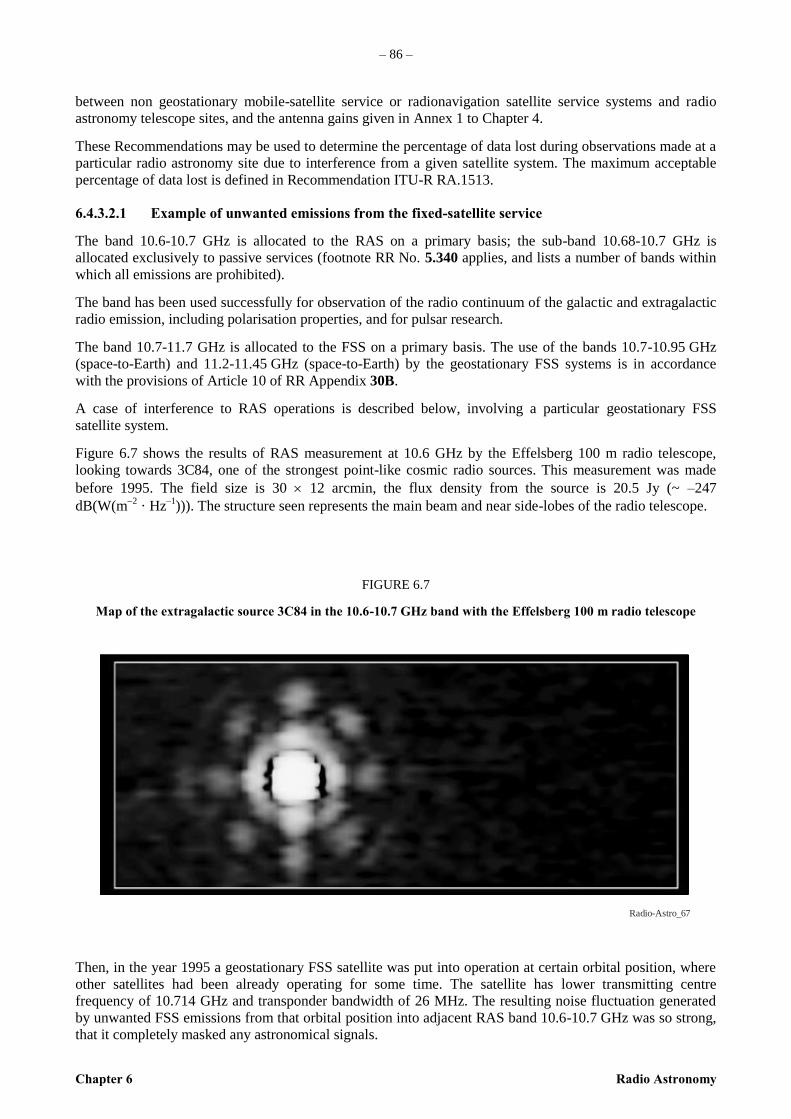
– 86 –
Chapter 6 Radio Astronomy
between non geostationary mobile-satellite service or radionavigation satellite service systems and radio
astronomy telescope sites, and the antenna gains given in Annex 1 to Chapter 4.
These Recommendations may be used to determine the percentage of data lost during observations made at a
particular radio astronomy site due to interference from a given satellite system. The maximum acceptable
percentage of data lost is defined in Recommendation ITU-R RA.1513.
6.4.3.2.1 Example of unwanted emissions from the fixed-satellite service
The band 10.6-10.7 GHz is allocated to the RAS on a primary basis; the sub-band 10.68-10.7 GHz is
allocated exclusively to passive services (footnote RR No. 5.340 applies, and lists a number of bands within
which all emissions are prohibited).
The band has been used successfully for observation of the radio continuum of the galactic and extragalactic
radio emission, including polarisation properties, and for pulsar research.
The band 10.7-11.7 GHz is allocated to the FSS on a primary basis. The use of the bands 10.7-10.95 GHz
(space-to-Earth) and 11.2-11.45 GHz (space-to-Earth) by the geostationary FSS systems is in accordance
with the provisions of Article 10 of RR Appendix 30B.
A case of interference to RAS operations is described below, involving a particular geostationary FSS
satellite system.
Figure 6.7 shows the results of RAS measurement at 10.6 GHz by the Effelsberg 100 m radio telescope,
looking towards 3C84, one of the strongest point-like cosmic radio sources. This measurement was made
before 1995. The field size is 30 12 arcmin, the flux density from the source is 20.5 Jy (~ –247
dB(W(m2
· Hz–1
))). The structure seen represents the main beam and near side-lobes of the radio telescope.
FIGURE 6.7
Map of the extragalactic source 3C84 in the 10.6-10.7 GHz band with the Effelsberg 100 m radio telescope
Radio-Astro_67
Then, in the year 1995 a geostationary FSS satellite was put into operation at certain orbital position, where
other satellites had been already operating for some time. The satellite has lower transmitting centre
frequency of 10.714 GHz and transponder bandwidth of 26 MHz. The resulting noise fluctuation generated
by unwanted FSS emissions from that orbital position into adjacent RAS band 10.6-10.7 GHz was so strong,
that it completely masked any astronomical signals.
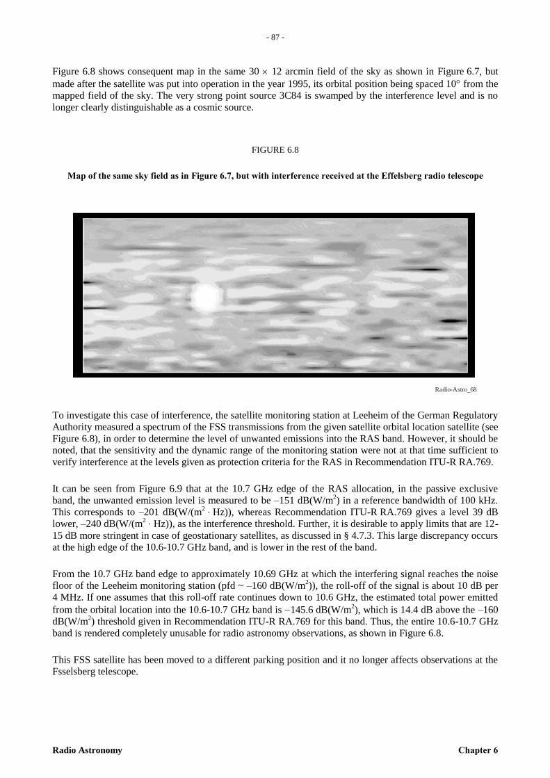
- 87 -
Radio Astronomy Chapter 6
– 8
7 –
Figure 6.8 shows consequent map in the same 30 12 arcmin field of the sky as shown in Figure 6.7, but
made after the satellite was put into operation in the year 1995, its orbital position being spaced 10 from the
mapped field of the sky. The very strong point source 3C84 is swamped by the interference level and is no
longer clearly distinguishable as a cosmic source.
FIGURE 6.8
Map of the same sky field as in Figure 6.7, but with interference received at the Effelsberg radio telescope
Radio-Astro_68
To investigate this case of interference, the satellite monitoring station at Leeheim of the German Regulatory
Authority measured a spectrum of the FSS transmissions from the given satellite orbital location satellite (see
Figure 6.8), in order to determine the level of unwanted emissions into the RAS band. However, it should be
noted, that the sensitivity and the dynamic range of the monitoring station were not at that time sufficient to
verify interference at the levels given as protection criteria for the RAS in Recommendation ITU-R RA.769.
It can be seen from Figure 6.9 that at the 10.7 GHz edge of the RAS allocation, in the passive exclusive
band, the unwanted emission level is measured to be –151 dB(W/m2) in a reference bandwidth of 100 kHz.
This corresponds to –201 dB(W/(m2 · Hz)), whereas Recommendation ITU-R RA.769 gives a level 39 dB
lower, –240 dB(W/(m2 · Hz)), as the interference threshold. Further, it is desirable to apply limits that are 12-
15 dB more stringent in case of geostationary satellites, as discussed in § 4.7.3. This large discrepancy occurs
at the high edge of the 10.6-10.7 GHz band, and is lower in the rest of the band.
From the 10.7 GHz band edge to approximately 10.69 GHz at which the interfering signal reaches the noise
floor of the Leeheim monitoring station (pfd ~ –160 dB(W/m2)), the roll-off of the signal is about 10 dB per
4 MHz. If one assumes that this roll-off rate continues down to 10.6 GHz, the estimated total power emitted
from the orbital location into the 10.6-10.7 GHz band is 145.6 dB(W/m2), which is 14.4 dB above the –160
dB(W/m2) threshold given in Recommendation ITU-R RA.769 for this band. Thus, the entire 10.6-10.7 GHz
band is rendered completely unusable for radio astronomy observations, as shown in Figure 6.8.
This FSS satellite has been moved to a different parking position and it no longer affects observations at the
Fsselsberg telescope.

– 88 –
Chapter 6 Radio Astronomy
FIGURE 6.9
Measurement of the geostationary FSS interference conducted at
Leeheim monitoring station (1995)
Radio-Astro_69
6.4.3.3 Potential cases of harmonic interference from satellites
6.4.3.3.1 Second harmonic radiation in the 23.6-24.0 GHz band from broadcasting satellites
A possible mode of interference to radio astronomy is second harmonic radiation from broadcasting satellites
in the band 11.7 to 12.5 GHz. The harmonic range 23.4 to 25.0 GHz includes the exclusive passive band 23.6
to 24.0 GHz. For Regions 1 and 3, Annex 3 of RR Appendix 30 lists for individual reception a minimum pfd
in the 11.7 to 12.5 GHz band of 103 dB(W/m2) at the edge of the coverage area, and the pfd in the centre of
the coverage area would normally be 100 dB(W/m2). These values of pfd are applicable to each channel of
the broadcasting-satellite service. The total pfd within the band 11.8-12.0 GHz band may reach a value of –
91 dB(W/m2).
According to Table 4.1, interference detrimental to radio astronomy would occur for signals greater than
147 dB(W/m2) in a bandwidth of 400 MHz at 24 GHz. For a side-lobe gain of 0 dBi for the radio astronomy
antenna, the required suppression of the second harmonic is thus 56 dB, which can be achieved with
established design techniques.
- 89 -
Radio Astronomy Chapter 6
– 8
9 –
6.4.3.3.2 Second-harmonic radiation near 22.2 GHz from the FSS
A situation similar to that discussed in § 6.4.3.2.1 exists for the radio astronomy water-vapour band at
22.2 GHz, but the permitted pfd’s at the Earth from transmitters in the fixed service are lower than in the
broadcasting-satellite service, and the interference problem is correspondingly less. This also applies to the
passive bands at 15.35-15.4 GHz and 164-168 GHz, which also contain second harmonics of frequencies
allocated to space-to-Earth transmissions.
6.4.3.3.3 Second-harmonic radiation in the 4 990-5 000 MHz band from the radiodetermination
satellite and mobile satellite band
The band 2 483.5-2 500 MHz has been allocated to the radiodetermination satellite and mobile satellite
services for downlink transmissions from satellites to user units. Second harmonics of such transmissions
extend over the worldwide primary radio astronomy band 4 990-5 000 MHz (4 950-5 000 MHz in Argentina,
Australia, and Canada). The detrimental threshold for interference to radio astronomy in the 4 990-
5 000 MHz band is –171 dB(W/m2) from Table 4.1.
6.4.3.3.4 Third-harmonic radiation in the 1 400-1 427 MHz band from the meteorological-satellite
service
Some meteorological satellites use the band 460-470 MHz for interrogation of platforms on the Earth to
obtain data that is then relayed to data-collection centres. The third harmonic of such transmissions above
466 MHz falls within the 1 400-1 427 MHz radio astronomy band. Powers up to 40 W are used for these
transmissions. With the assumption of a geostationary satellite with 0 dBi gain in the transmitting antenna at
the third harmonic, the pfd at the subsatellite point on the Earth is 146 dB(W/m2). For reception in the 0 dBi
side-lobes of the radio astronomy antenna the harmonic suppression must be at least –34 dB relative to the
fundamental transmission intensity.
6.5 Unwanted emissions from wideband modulation
See Recommendation ITU-R RA.1237 – Protection of the RAS from unwanted emissions resulting from
applications of wideband digital modulation.
6.5.1 Usage of broadband modulation
In certain types of transmissions often associated with digital data, spectral sidebands are generated over a
much broader frequency range than is used in reception of the signals. In particular, digital phase-shift
keying modulation techniques produce a power spectrum of the form [sin(x)/x]2 with recurring subsidiary
maxima outside the wanted band, which decrease only slowly with frequency. Although, in general, only the
central maximum of the spectrum is used in reception by the service concerned, the sidebands are sometimes
radiated without effective filtering. The envelope of the unfiltered sidebands, for example, at 10 times the –3
dB spectral bandwidth from the centre frequency, is reduced by only 29 dB below the power level at the
central maximum. If, in addition, the keying frequency of a transmission with binary phase-shift keying
(BPSK) is 10-20 MHz, then these ten bandwidths extend over several hundred megahertz around the
assigned frequency. For example, consider a simple unfiltered BPSK transmitter with a keying frequency of
10 MHz centred on 1 615 MHz, and an output power of 40 W radiating through an isotropic antenna
mounted on an aircraft. At a LoS distance of 400 km from an observatory, unwanted sidebands would result
in a pfd level at the spectral maxima in the 1 400-1 427 MHz radio astronomy band that is 48 dB above the
corresponding detrimental threshold level in Table 4.1. Emission in the 1 610.6-1 613.8 MHz and 1 660-1 670
MHz bands, which are also allocated to radio astronomy, would be at a significantly higher level.
PSK is also used in direct-sequence spread-spectrum modulation. A characteristic common to most spread-
spectrum techniques is a wide-band signal with low power spectral density. This characteristic reduces the
probability of such transmissions causing interference to conventional narrow-band communications
systems, in which the only interest is in retrieving the modulation from a signal. In contrast, the concern in
radio astronomy is in precisely measuring the power received from natural sources. Cosmic radio waves
generally have the characteristics of random noise, and wide receiver bandwidths must often be used to
provide the required sensitivity. Thus, there is often no way to distinguish between spread spectrum signals
– 90 –
Chapter 6 Radio Astronomy
and cosmic signals. The detrimental thresholds of pfd for interference to radio astronomy in Chapter 4 apply
to unwanted as well as to intentional emissions, and to all types of modulation including those
discussed above.
6.5.2 Pulse shaping to reduce unwanted emissions
The levels of unwanted emissions from digital modulation can be greatly reduced by pulse shaping, that is,
by using pulse shapes that avoid sharp near-rectangular transitions in amplitude or phase. A theorem of
Fourier transforms indicates that if the pulse shape as a function of time becomes impulsive at the n-th
derivative, then in the power spectrum the sidebands fall off as the inverse frequency to the power 2n. In the
case of rectangular pulses in the time domain, the pulse shape function becomes impulsive at the first
derivative (n 1), and the sidebands fall off as f –2
, as in the sinc-squared form mentioned above. As an
example of pulse shaping consider the case of pulses in which the rectangular transitions of unit amplitude
are replaced by [1 sin (x)]/2 where x goes linearly from /2 to /2 for positive transitions and /2 to –/2
for negative ones. The resulting pulse waveform becomes impulsive at the third derivative, and hence the
power spectrum falls off as f –6
. This result has been demonstrated [Ponsonby, 1994]. Thus, for example, at a
frequency where the envelope of the power spectrum has fallen to –20 dB relative to the maximum for
rectangular pulses, it would have fallen to –60 dB with the sinusoidal shaping just described. Such a result is
very helpful, since the spectral range over which modulation-induced unwanted emissions could be
detrimental to radio astronomy is greatly reduced. Numerous other practical forms of pulse shaping to reduce
unwanted emissions have been described; for example, Gaussian-filtered minimun shift keying (GMSK)
[Murota and Hirade, 1981; Otter, 1994].
Use of modulation techniques designed to minimize unwanted emissions can be effective only if the power
amplifier stages following the modulator are sufficiently linear to avoid generating unwanted emissions as
intermodulation products. This is a particular problem for satellite transmissions for which the limits on
electrical power may lead to maximization of the transmitter efficiency at the expense of linearity. In some
communications satellites a number of different beams are used for the downlink transmissions to allow
frequency re-use. The beams are formed by appropriate phasing of a large number of radiating elements,
each of which is driven by a separate power amplifier. Filtering of the amplified signals to remove unwanted
emissions is not always considered practical in such cases.
6.5.3 Example of interference from broadband modulation.
The GLONASS series of radiodetermination satellites [Daly, 1988; Ponsonby, 1991], have been a source of
interference to radio astronomy observations in the bands 1 610.6-1 613.8 MHz and 1 660-1 670 MHz since
the mid 1980s [Galt, 1990]. The fully deployed system includes 24 satellites in three orbital planes. Initially
24 transmission channels with centre frequencies spaced at intervals of 0.5625 MHz from 1 602.5625 MHz
to 1 615.5 MHz were planned to be used. Interference is caused by satellites with channels well outside the
radio astronomy bands as a result of sidebands from the spread spectrum modulation. The sidebands show a
structure in their frequency spectrum which recurs at intervals of 0.511 and 5.11 MHz resulting from the
keying frequencies of the low- and high-precision code modulations respectively. The main structure in the
sidebands is the series of maxima spaced at 5.11 MHz, and narrow spikes in frequency that occur in some of
the nulls. Some of the null spikes can be found at frequencies as far from the transmit channel as the
1 660-1 670 MHz radio astronomy band.
A sequence of tests was executed by the GLONASS administration working in collaboration with IUCAF, in
November 1992. Satellites using transmission channels close to the 1 610.6-1 613.8 MHz band were shifted
in frequency or turned off in stages. Fifteen observatories around the world assisted in evaluating the effects
of these GLONASS system modifications on the quality of the astronomical data. The evaluation of the
results formed the basis for formal agreements between the GLONASS administration, IUCAF, and several
national governments, describing a comprehensive solution to the GLONASS interference problem in the
radio astronomy bands. This solution consists of:
– a reduction of the number of required frequency channels by using the same channel for antipodal
satellites;
– a downward shift in assigned channel frequencies away from the radio astronomy band; and
– the application of filtering above the first null in the spread spectrum of the highest frequency channel.
- 91 -
Radio Astronomy Chapter 6
– 9
1 –
Since the GLONASS-IUCAF agreement, no spacecraft with frequency capacity higher than 1 610 MHz have
been launched, and all have OoB filters; after 1999 the main emissions in the 1 612 MHz radio astronomy
band have been eliminated. The GLONASS-IUCAF agreement has been explicitly recognized in the Radio
Regulations i.e. Table 1-2 of Annex 1 to Res 739 (Rev.WRC-07) states: "This Resolution does not apply to
current and future assignments of the radionavigation satellite system GLONASS/GLONASS-M in the band
1 559-1 610 MHz, irrespective of the date of reception of the related coordination or notification
information, as appropriate. The protection of the radio astronomy service in the 1 610.6 -1 613.8 MHz band
is ensured and will continue to be in accordance with the bilateral agreement between the Russian
Federation, the notifying administration of the GLONASS/GLONASS-M system, and IUCAF, and
subsequent bilateral agreements with other administrations."
6.5.4 Example: Radio interference from the IRIDIUM (HIBLEO-2) MSS system
This section is derived from ECC Report 171, where extensive details of the methodology and measurements
are provided.
6.5.4.1 RAS operations in the band 1610.6-1613.8 MHz
The 1 610.6-1 613.8 MHz band is allocated to the radio astronomy service on a primary basis. It used for
spectral line observations of the hydroxyl radical (OH). The OH transition at rest frequency 1 612 MHz is
one of the most important spectral lines for RAS, and is listed as such in Recommendation ITU-R RA.314.
OH was the first cosmic radical to be detected at radio frequencies (1963) and continues to be a powerful
research tool. In its ground state the OH molecule produces four spectral lines, at frequencies of
approximately 1 612, 1 665, 1 667 and 1 720 MHz, all of which have been observed in emission and in
absoprtion in our Galaxy, as well as in external galaxies. The study of OH lines provides information on a
wide range of astronomical phenomena, e.g. the formation of protostars and the evolution of stars. To
interpret most observations made of the OH molecule, it is necessary to measure the relative strength of
several of these lines. The loss of the ability to observe any one of these lines will prevent the study of these
classes of physical phenomena.
6.5.4.2 IRIDIUM constellation description
The Mobile-Satellite Service (Earth-to-Space) is allocated in the band 1610.0 - 1626.5 MHz and the Mobile-
Satellite (Space-to-Earth) has a secondary allocation in the band 1613.8 – 1626.5 MHz. Footnote 5.208B
stipulates that Resolution 739 (WRC-07) applies to future systems planned for this band.
The IRIDIUM system employs 66 Low Earth Orbit (LEO) satellites that support user-to-user, user-to-
gateway, and gateway-to-gateway communications. The 66 satellites are evenly distributed in six orbital
planes with a 86.4° inclination, with one in-orbit spare for each orbital plane. Except for planes 1 and 6, the
orbital planes are co-rotating planes spaced 31.6° apart. The first and last orbital planes are spaced 22° apart
and form a seam where the satellites are counter-rotating. The satellites orbit at an altitude of 780 km and
have an orbital period of approximately 100 min 28 s.
They communicate in the band 1618.25 – 1626.5 MHz with special mobile equipment on the ground and in
the air and provide a global communications service that reaches all locations on our planet.
6.5.4.3 Nature and characteristics of the IRIDIUM interference.
Theoretical predictions carried out in 1998 with the Iridium (HIBLEO-2) constellation under artificial full-
load conditions have been summarised in ITU-R Recommendation SM.1633 (2003), Annex 6:
“4.2 Calculation of the interference level
Unwanted emissions in terms of aggregate spfd of HIBLEO-2 satellite transmissions in the 1 610.6-1 613.8
MHz band have been theoretically estimated to range between -214 dB(W/(m2/Hz)) and -223 dB(W/(m
2/Hz))
at some radio astronomy sites, under fully loaded conditions."
The IRIDIUM satellite interference in the band 1610.6 -1613.8 MHz is caused by 7th order intermodulation
products generated on the satellite and not by overloading of radio astronomical receivers. Analysis of
spectra of the interference taken at the Effelsberg telescope (report from 1.3.2006) shows that the two
fundamental Iridium carriers at f1 = 1618.25 MHz and f2= 1620.25 MHz produce the observed interference at
1612.25 MHz, which corresponds to the intermod relation f1 – 3df = 4f1 - 3f2 and suggests a 4 + 3 = 7-th

– 92 –
Chapter 6 Radio Astronomy
order IM product. No evidence was found of any lower order products at 1.61425 and 1.61625 GHz.
Ordinary amplifiers and mixers would produce an interference pattern where the power in IM products
decreases with increasing order. These low (3-5) IM orders are evidently suppressed by signal processing on
board the IRIDIUM satellite while high order IM products are still evident.
State-of-the-art microwave amplifiers and radio astronomical receivers have third order intercept points
(IIP3) at -30 to -25 dBm. A main carrier of –178 dBm of the IRIDIUM satellite (as observed) cannot create
detectable self-interference in a radio astronomical receiver frontend. The strength of the interference
allows an estimate of the 7th order intercept for the satellite transmitter of about +19dBW, which is close to
the satellite e.i.r.p. of +11 dBW. This suggests that the satellite transmitter has been driven into compression
will produce strong out of band emissions on both sides of the IRIDIUM band. For certain transmission
channel allocations, the 7th order intermodulation products will fall into the RAS band.
6.5.4.4 Measurements and verification
A collaborative test program, conducted by HIBLEO-2 (Iridium) and the United States National
Radio Astronomy Observatory (NRAO) in 1998, measured spfd values ranging from ‒220 to
‒240 dB(W/(m2/Hz)) at these sites. These values refer to the so-called voice channels that are turned on
when communication takes place. In addition the HIBLEO-2 system was found to radiate broadcast signals
at all times. The spectra of the broadcasting channels showed 9-10 narrow (less than 40 kHz wide) peaks
within the radio astronomy band. spfd peak values appeared to average ‒227 dB(W/(m2/Hz)) over 90 ms.
(Source: ITU-R Recommendation SM.1633 (2003) as cited in ECC Report 171).
6.5.4.5 Measurements at Leeheim MS on 8-9.6.2010
The Leeheim Space Radio Monitoring Station is located approximately 35 km south-west of Frankfurt/Main.
The Leeheim MS has a number of satellite antennas including a 12 m parabolic reflector Antenna 1 designed
to cover the 1 -13 GHz frequency range, with which the monitoring was done. High-precision angular
pointing allowed for accurate tracking of moving satellites.
The main measurement campaign at Leeheim was jointly carried out by MPIfR, ASTRON and BNetzA on
Iridium satellites on 8th and 9th June, 2010.Measurements were taken once per second in 6.1 kHz channels
in the range 1610.6-1613.8 MHz from 28 satellite passes of the Iridium constellation, observed between
08:30 and 17:30 (local time) over two days.
A 70 dB stop-band filter was used in front of the receiver to suppress the strong satellite emissions in the
1613.8 – 1626.5 MHz band in order to avoid non-linearities of the receiving system when the antenna
tracked an active satellite.
Calibrations were made directly on radio sources Cas-A and Cyg-A on the same day, using the same
configuration as for the satellite measurements thus providing an absolute flux density calibration of all
spectrometer channels.
A typical example of the spectra that were obtained is shown in Figure 6.10. The observed interference in the
RAS band has the same peak characteristics as those reported in SM.1633 dating from 1998. The peak
emission values obtained in the Leeheim MS measurements are comparable with those predicted
theoretically for fully loaded conditions, where -214 dB(W/m2Hz) translates into 40 kJy.
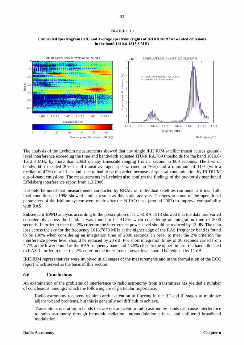
- 93 -
Radio Astronomy Chapter 6
– 9
3 –
FIGURE 6.10
Calibrated spectrogram (left) and average spectrum (right) of IRIDIUM 97 unwanted emissions
in the band 1610.6-1613.8 MHz
Radio-Astro_610
Fequency (MHz)
MPIFR AFFTS 2010-02-25T13:03:56.1561GPS
Spectral power flux density (dB (Jy))
1 611 1 611.5 1 612 1 612.5 1 613 1 613.5
0
100
200
300
400
500
600
1 610.5 1 611 1 611.5 1 612 1 612.5 1 613 1 613.5 1 614
Frequency (MHz)
MPIFR AFFTS 2010-02-25T13:03:56.1561GPS
Tim
e (
s)
0 10 20 30 40 50 60
0
1
2
3
4
5
6
7
8
910
4
ITU-R RA 769 threshold = 498.0429 Jy
exceeded in 456 of 525 channels
Speci
al
pow
er
flu
x d
ensi
ty (
Jy)
The analysis of the Leeheim measurements showed that any single IRIDIUM satellite transit causes ground-
level interference exceeding the time and bandwidth adjusted ITU-R RA.769 thresholds for the band 1610.6-
1613.8 MHz by more than 20dB on any timescale ranging from 1 second to 800 seconds. The loss of
bandwidth exceeded 30% in all transit averaged spectra (median 76%) and a minimum of 11% (with a
median of 47%) of all 1 second spectra had to be discarded because of spectral contamination by IRIDIUM
out-of-band emissions. The measurements in Leeheim also confirm the findings of the previously mentioned
Effelsberg interference report from 1.3.2006.
It should be noted that measurements conducted by NRAO on individual satellites run under artificial full-
load conditions in 1998 showed similar results as this static analysis. Changes to some of the operational
parameters of the Iridium system were made after the NRAO tests (around 2003) to improve compatibility
with RAS.
Subsequent EPFD analysis according to the prescription of ITU-R RA 1513 showed that the data loss varied
considerably across the band. It was found to be 93.2% when considering an integration time of 2000
seconds. In order to meet the 2% criterion the interference power level should be reduced by 13 dB. The data
loss across the sky for the frequency 1613.7878 MHz at the higher edge of the RAS frequency band is found
to be 100% when considering an integration time of 2000 seconds. In order to meet the 2% criterion the
interference power level should be reduced by 20 dB. For short integration times of 30 seconds varied from
4.7% at the lower bound of the RAS frequency band and 43.5% close to the upper limit of the band allocated
to RAS. In order to meet the 2% criterion the interference power level should be reduced by 11 dB.
IRIDIUM representatives were involved in all stages of the measurements and in the formulation of the ECC
report which served as the basis of this section.
6.6 Conclusions
An examination of the problems of interference to radio astronomy from transmitters has yielded a number
of conclusions, amongst which the following are of particular importance.
– Radio astronomy receivers require careful attention to filtering in the RF and IF stages to minimize
adjacent-band problems, but this is generally not difficult to achieve.
– Transmitters operating in bands that are not adjacent to radio astronomy bands can cause interference
to radio astronomy through harmonic radiation, intermodulation effects, and unfiltered broadband
modulation.
– 94 –
Chapter 6 Radio Astronomy
– Transmitters on satellites or aircraft can pose particular difficulties because LoS propagation
conditions generally exist and the probability of reception in side-lobes near the main beam (rather
than the far side-lobes) is greater than for terrestrial transmissions.
– In general, allocating bands adjacent to radio astronomy bands to services using high-powered
terrestrial transmissions or transmitters on satellites may lead to difficult and expensive technical
problems.
– Broadband emissions from satellites, such as signals using direct-sequence spread-spectrum
modulation, can result in particularly serious problems for radio astronomy unless such transmissions
are adequately filtered. Such unwanted emissions can be greatly reduced by the use of pulse-shaping
modulation techniques.
REFERENCES
DALY, P. [1988] Aspects of the Soviet Union’s Glonass satellite navigation system.
J. of Navigation, Vol. 41, p. 186-198.
GALT, J. [1990] Contamination from satellites. Nature, Vol. 345, p. 483.
MUROTA, K and HIRADE, K. [1981] GMSK modulation for digital mobile radio telephony.
IEEE Trans. Commun., Vol. COM-29, p. 1044-1050.
OTTER, M. A. [June 1994] A comparison of QPSK, OQPSK, BPSK and GMSK modulation schemes.
Report of the European Space Agency, European Space Operations Center, Darmstadt, Germany.
PONSONBY, J. E. B. [July 1991] Spectrum management and the impact of the GLONASS and GPS satellite
systems on Radioastronomy. J. of Navigation, Vol. 44, p. 392-398.
PONSONBY, J. E. B. [July 1994] Impact of the direct sequence spread spectrum signals from the Global
Satellite Navigation System GLONASS on radio astronomy: problem and proposed solution. Proc. of the
IEEE Spread Spectrum Symposium, Oulu, Finland.
- 95 -
Radio Astronomy Chapter 7
– 9
5 –
CHAPTER 7
Special techniques, applications and observing locations
7.1 Introduction
This Chapter discusses techniques and observing locations that are not fully covered by the more general
considerations in earlier Chapters. In particular, certain applications of radio astronomy involve observation
with one or more antennas in space, and are sometimes referred to as space radio astronomy. The reasons
why an antenna in space is required include:
– In VLBI, correlation of signals from terrestrial antennas with signals from an antenna in space
provides longer baselines, and thus greater angular resolution, than can be achieved using terrestrial
antennas alone. The motion of the space antenna in an orbit about the Earth provides variation in
the directions of the baselines that it forms with the terrestrial antennas, which is important for two-
dimensional imaging.
– For observation and measurement of the structure of the cosmic microwave background (CMB)
radiation, very high sensitivity is required at frequencies of approximately 30 GHz and higher.
Avoiding atmospheric absorption, and in particular the variations in signal strength resulting from
atmospheric irregularities is very important, especially for single antenna (total power)
measurements.
– For frequencies close to those of the strong absorption lines of H2O and O2 in the Earth’s
atmosphere (see Figure 3.1), observations from space are necessary.
– For observations at low frequencies, at which radio waves cannot penetrate the ionosphere or are
strongly attenuated, observations from space are also necessary.
The most important locations of space antennas for radio astronomy are as follows:
– Earth orbit, especially useful for VLBI (see § 7.2).
– The L2 Sun-Earth Lagrangian point (see § 7.3), approximately 1.5 106 km from Earth and thus
providing some protection from terrestrial interference.
– Earth-trailing orbits in which the satellite is close to the Earth’s orbit around the Sun but trails the
Earth by a distance typically 106-10
7 km, again providing some protection from terrestrial
interference.
– The shielded zone of the Moon, (see § 7.4) which provides the most effective protection from
terrestrial interference but has not yet been used.
The L2 point, the shielded zone of the Moon, and most planned Earth orbits all lie within the 2 106 km
distance that defines the boundary between near-Earth space and deep space. Earth orbits and the L2 point
have been used in observations of the structure of the CMB radiation. Terrestrial sites chosen for the lowest
atmospheric water vapour, the South Pole and the Atacama desert, have also been used for CMB
observations (see § 7.5).
Other special techniques and applications discussed in this chapter include geodetic measurements using
VLBI (see § 7.2.2), observation of pulsars, which have possible applications in timekeeping (see § 7.6) and
observations of the Sun and its effects on space weather (see § 7.7).
– 96 –
Chapter 7 Radio Astronomy
7.2 VLBI, including Space VLBI
The VLBI technique involves simultaneous observations of a radio source using antennas separated by large
distances, often in different countries or in Earth orbit. The angular resolution for VLBI observations is
unsurpassed by any other ground-based astronomical technique. VLBI arrays with maximum baselines
approaching the diameter of the Earth can achieve an angular resolution of less than one milli-arcsecond.
Precisely matched observing frequencies can be achieved at the antennas of a VLBI array using highly stable
atomic clocks to maintain phase coherence without a real-time reference link. When hydrogen masers are
used as clocks, the coherent integration time is generally limited only by differential variations in path length
through the atmosphere and ionosphere. However, at high frequencies the stability of the masers (10–14
) can
be the limiting factor; for instance, at 100 GHz it would limit the coherent integration time to 1 000 s. The
data obtained at the individual antenna sites are either recorded (currently on magnetic disks) or transmitted
via high-speed wide-area networks. Recorded or transmitted data rates depend on the scientific goals and
observing procedures, and on the available technical facilities. Maximum rates used in current practice are
approaching 2 Gigabit/sec, which is a new standard adopted by the Very Long Baseline Array (VLBA), a
dedicated VLBI instrument with ten observing stations distributed across the breadth of the United States of
America. A central processing facility aligns the reproduced signals in time, allowing for the substantial
light-travel delay of up to 20 milliseconds, and combines all pairs of signals to form correlation products.
The resolution of the VLBI technique enables radio astronomers to observe relative motions of individual
condensations of high-energy plasmas being ejected at relativistic velocities from active galactic nuclei.
Within the Milky Way Galaxy, VLBI can measure parallax-based distances across the entire Galactic disk,
and an intensive observing program is now surveying the spiral structure of the Galaxy with unprecedented
accuracy. VLBI is a major component in the definition of celestial and terrestrial reference frames, and
standard times, and has important applications in other areas ranging from the motion of the Earth’s crustal
plates to precise angular positioning of distant spacecraft.
The sensitivity of VLBI networks to interference from active services is discussed in § 4.4 and the use of
certain frequency bands is discussed in § 5.8.
7.2.1 Space VLBI
Space VLBI extends the VLBI technique’s resolution beyond the limits imposed by the size of the Earth, by
including an antenna in a high orbit around the Earth in the observing array. The following subsections
review past, current, and planned future missions (§ 7.2.1.1), the instrumental features unique to Space VLBI
(§ 7.2.1.2), and in particular the technique’s requirements for communication frequencies (§ 7.2.1.3).
7.2.1.1 Space VLBI projects
Table 7.1 summarizes the basic parameters of the Space VLBI projects described in this section.
Frequencies cited in the table and the subsequent discussions refer to the radio emissions received from
natural cosmic radio sources.
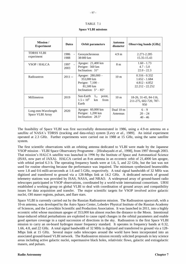
- 97 -
Radio Astronomy Chapter 7
– 9
7 –
TABLE 7.1
Space VLBI missions
The feasibility of Space VLBI was first successfully demonstrated in 1986, using a 4.9-m antenna on a
satellite of NASA’s TDRSS (tracking and data-relay) system [Levy et al., 1989]. An initial experiment
operated at 2.3 GHz. Further experiments were carried out in 1988 at 15 GHz, using the same satellite
system.
The first scientific observations with an orbiting antenna dedicated to VLBI were made by the Japanese
VSOP mission – VLBI Space Observatory Programme – [Hirabayashi et al., 1998], from 1997 through 2003.
That mission’s HALCA satellite was launched in 1996 by the Institute of Space and Astronautical Science
(ISAS, now part of JAXA). HALCA carried an 8-m antenna in an eccentric orbit of 21,4000 km apogee,
with orbital period 6.3 h. The operating frequency bands were at 1.6, 5, and 22 GHz, but the last was not
used for routine observing because the performance was impaired. The minimum synthesized beamwidths
were 1.8 and 0.6 milli-arcseconds at 1.6 and 5 GHz, respectively. A total signal bandwidth of 32 MHz was
digitized and transferred to ground via a 128-Mbps link at 14.2 GHz. A dedicated network of ground
telemetry stations was provided by ISAS, NASA, and NRAO. A widespread array of ground-based radio
telescopes participated in VSOP observations, coordinated by a world-wide international consortium. URSI
established a working group on global VLBI to deal with coordination of ground arrays and compatibility
issues for data acquisition and transfer. The major scientific targets for VSOP involved active galactic
nuclei, OH maser regions, pulsars, and flare stars.
Space VLBI is currently carried out by the Russian Radioastron mission. The Radioastron spacecraft, with a
10-m antenna, was developed by the Astro Space Center, Lebedev Physical Institute of the Russian Academy
of Sciences, and the Lavochkin Scientific and Production Association. It was launched in 2011, into a highly
eccentric orbit whose maximum apogee of 353,000 km almost reaches the distance to the Moon. Intentional
lunar-induced orbital perturbations are exploited to cause rapid changes in the orbital parameters and enable
good aperture coverage in a rapid succession of directions in the sky. Radioastron is the first Space VLBI
mission to carry an on-board hydrogen maser frequency standard. It operates in frequency bands at 0.32,
1.66, 4.8, and 22 GHz. A total signal bandwidth of 32 MHz is digitized and transferred to ground via a 128-
Mbps link at 15 GHz. Several major radio telescopes around the world have been incorporated into an
associated ground-based VLBI network. The Radioastron mission recently solicited proposals in key science
areas including active galactic nuclei, supermassive black holes, relativistic flows, galactic and extragalactic
masers, and pulsars.
Mission /
Experiment Dates Orbit parameters
Antenna
diameter Observing bands [GHz]
TDRSS VLBI
experiment 1986 -
1988
Geosynchronous
38 000 km
4.9 m 2.271-2.285
15.35-15.43
VSOP / HALCA 1997 -
2003
Apogee: 21,400 km
Perigee: 560 km
Inclination: 31°
8 m 1.60 - 1.73
4.7 - 5.0
22.0 - 22.3
Radioastron 2011 -- Apogee: 280,000 –
353,000 km
Perigee: 7,100 –
81,500 km
Inclination: 5° – 85°
10 m 0.316 - 0.332
1.652 - 1.684
4.812 - 4.852
22.212 - 22.252
Millimetron 2019 Sun-Earth L2 point,
1.5 106 km from
Earth
10 m 18-26, 31-45, 84-116,
211-275, 602-720, 787-
950
Long-mm-Wavelength
Space VLBI Array
2020 Apogee: 60,000 km
Perigee: 1,200 km
Inclination: 28.5°
Dual 10-m
Antennas
6 – 9
20 – 24
40 - 46
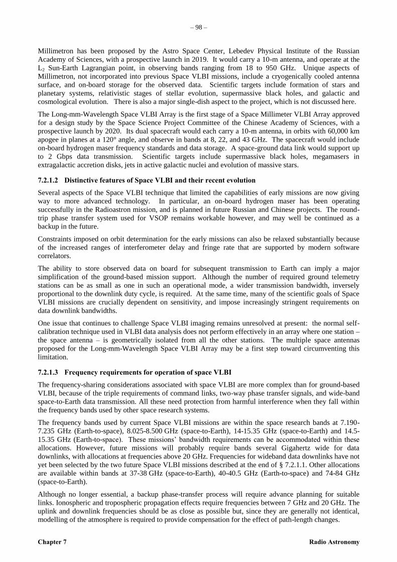
– 98 –
Chapter 7 Radio Astronomy
Millimetron has been proposed by the Astro Space Center, Lebedev Physical Institute of the Russian
Academy of Sciences, with a prospective launch in 2019. It would carry a 10-m antenna, and operate at the
L2 Sun-Earth Lagrangian point, in observing bands ranging from 18 to 950 GHz. Unique aspects of
Millimetron, not incorporated into previous Space VLBI missions, include a cryogenically cooled antenna
surface, and on-board storage for the observed data. Scientific targets include formation of stars and
planetary systems, relativistic stages of stellar evolution, supermassive black holes, and galactic and
cosmological evolution. There is also a major single-dish aspect to the project, which is not discussed here.
The Long-mm-Wavelength Space VLBI Array is the first stage of a Space Millimeter VLBI Array approved
for a design study by the Space Science Project Committee of the Chinese Academy of Sciences, with a
prospective launch by 2020. Its dual spacecraft would each carry a 10-m antenna, in orbits with 60,000 km
apogee in planes at a 120° angle, and observe in bands at 8, 22, and 43 GHz. The spacecraft would include
on-board hydrogen maser frequency standards and data storage. A space-ground data link would support up
to 2 Gbps data transmission. Scientific targets include supermassive black holes, megamasers in
extragalactic accretion disks, jets in active galactic nuclei and evolution of massive stars.
7.2.1.2 Distinctive features of Space VLBI and their recent evolution
Several aspects of the Space VLBI technique that limited the capabilities of early missions are now giving
way to more advanced technology. In particular, an on-board hydrogen maser has been operating
successfully in the Radioastron mission, and is planned in future Russian and Chinese projects. The round-
trip phase transfer system used for VSOP remains workable however, and may well be continued as a
backup in the future.
Constraints imposed on orbit determination for the early missions can also be relaxed substantially because
of the increased ranges of interferometer delay and fringe rate that are supported by modern software
correlators.
The ability to store observed data on board for subsequent transmission to Earth can imply a major
simplification of the ground-based mission support. Although the number of required ground telemetry
stations can be as small as one in such an operational mode, a wider transmission bandwidth, inversely
proportional to the downlink duty cycle, is required. At the same time, many of the scientific goals of Space
VLBI missions are crucially dependent on sensitivity, and impose increasingly stringent requirements on
data downlink bandwidths.
One issue that continues to challenge Space VLBI imaging remains unresolved at present: the normal self-
calibration technique used in VLBI data analysis does not perform effectively in an array where one station –
the space antenna – is geometrically isolated from all the other stations. The multiple space antennas
proposed for the Long-mm-Wavelength Space VLBI Array may be a first step toward circumventing this
limitation.
7.2.1.3 Frequency requirements for operation of space VLBI
The frequency-sharing considerations associated with space VLBI are more complex than for ground-based
VLBI, because of the triple requirements of command links, two-way phase transfer signals, and wide-band
space-to-Earth data transmission. All these need protection from harmful interference when they fall within
the frequency bands used by other space research systems.
The frequency bands used by current Space VLBI missions are within the space research bands at 7.190-
7.235 GHz (Earth-to-space), 8.025-8.500 GHz (space-to-Earth), 14-15.35 GHz (space-to-Earth) and 14.5-
15.35 GHz (Earth-to-space). These missions’ bandwidth requirements can be accommodated within these
allocations. However, future missions will probably require bands several Gigahertz wide for data
downlinks, with allocations at frequencies above 20 GHz. Frequencies for wideband data downlinks have not
yet been selected by the two future Space VLBI missions described at the end of § 7.2.1.1. Other allocations
are available within bands at 37-38 GHz (space-to-Earth), 40-40.5 GHz (Earth-to-space) and 74-84 GHz
(space-to-Earth).
Although no longer essential, a backup phase-transfer process will require advance planning for suitable
links. Ionospheric and tropospheric propagation effects require frequencies between 7 GHz and 20 GHz. The
uplink and downlink frequencies should be as close as possible but, since they are generally not identical,
modelling of the atmosphere is required to provide compensation for the effect of path-length changes.

- 99 -
Radio Astronomy Chapter 7
– 9
9 –
The protection criteria for telecommunication links for manned and unmanned near-Earth research satellites
are listed in Recommendation ITU-R SA.609. These are also appropriate for the telemetering and timing
links of planned space VLBI systems. The recommended harmful interference thresholds, to be exceeded no
more than 0.1% of the time, are –216 dB(W/Hz) at the Earth station receiver, and –177 dB(W/kHz) at the
satellite receiver. The frequency bands to be used for the communication links of planned space VLBI
projects are allocated to many radiocommunication services. However, consideration of the potential
interference levels as a function of orbital position of the satellites indicates that effective sharing is possible.
In some cases, careful coordination may be required.
7.2.2 Geodetic applications using VLBI
VLBI is an essential tool in measuring and monitoring the Earth. Given a network of antennas at different
locations around the world, and a system of radio sources with accurately determined positions, distances
between pairs of antennas can be determined with an accuracy of a few millimetres. VLBI is the only
geodetic technique capable of providing a full set of Earth Orientation Parameters (EOPs: length of day and
orientation of the pole) which place the Earth with respect to the inertial Celestial Reference Frame (CRF),
described by a catalogue of quasars. By measuring the EOPs, VLBI provides an absolute orientation and
scale for the Terrestrial Reference Frame (TRF). The EOPs are essential for spacecraft navigation but they
change on short timescales and are not predictable, so they require regular measurement. Calibration of GPS
satellite data would not be possible without VLBI for example. The International VLBI Service (IVS) for
Geodesy and Astrometry (Schuh and Behrend 2012) are charged with the mission of maintaining the CRF
and providing regular measurement of the EOPs.
In recent years a plan has been formulated to modernise the network of telescopes contributing to IVS to
meet some challenging goals, including accuracies of 1 mm in position and 0.1 mm/y in velocity
[Petrachenko et al, 2013]. This initiative, termed the VLBI2010 Global Observing System (VGOS) requires
new small, fast moving telescopes and broadband receiving systems. Some new telescopes have already been
built (e.g. the AuScope VLBI Array, Lovell et al., 2013), are under construction or are planned. Broadband
receiving systems are required to provide both the frequency coverage and sensitivity required to meet the
VGOS goals. Observatories will record four dual-polarisation bands 1 GHz wide spread between 2 and
14 GHz.
7.3 Radio astronomy from the L2 Sun-Earth Lagrangian point
There are five special libration (Lagrangian) points in the gravitational field of the Sun-Earth system around
which stable (halo) orbits can be established for spacecraft. The positions are useful for establishing
permanent laboratories in space. The L1 and L2 points are located along the Sun-Earth line, at distances of
approximately 1.5 106 km each side the Earth, see Figure 7.1. The L2 point is further from the Sun, and at
this location the LoSs to the Sun, Earth and Moon lie within a few degrees of each other. The diameter of the
geostationary orbit around the Earth subtends an angle of approximately 3.1 from the L2 point, so an
antenna with low back side-lobes, pointing away from the earth, could be well protected from most
transmitters in the vicinity of the Earth. This consideration, and other advantages such as the favourable
conditions in space for maintaining low physical temperatures of the antenna and receiving equipment, have
led to proposals for a number of astronomical missions to be located in orbit around the L2 point. Preliminary
data for several of these are listed in Table 7.2. Protection of the electromagnetic environment near the L2
point is the subject of Recommendation ITU-R RA.1417, which recommends that a volume of space of
radius 250 000 km centred on the L2 point should be protected as a coordination zone of low electromagnetic
emission.
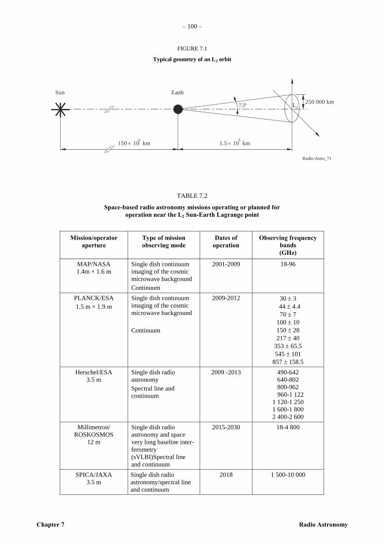
– 100 –
Chapter 7 Radio Astronomy
FIGURE 7.1
Typical geometry of an L2 orbit
Radio-Astro_71
150 10 km6
EarthSun
7.5° 250 000 km
L2
1.5 10 km6
TABLE 7.2
Space-based radio astronomy missions operating or planned for
operation near the L2 Sun-Earth Lagrange point
Mission/operator
aperture
Type of mission
observing mode
Dates of
operation
Observing frequency
bands
(GHz)
MAP/NASA
1.4m × 1.6 m
Single dish continuum
imaging of the cosmic
microwave background
Continuum
2001-2009
18-96
PLANCK/ESA
1.5 m × 1.9 m
Single dish continuum
imaging of the cosmic
microwave background
Continuum
2009-2012
30 3
44 4.4
70 7
100 10
150 28
217 40
353 65.5
545 101
857 158.5
Herschel/ESA
3.5 m
Single dish radio
astronomy
Spectral line and
continuum
2009 -2013
490-642
640-802
800-962
960-1 122
1 120-1 250
1 600-1 800
2 400-2 600
Millimetron/
ROSKOSMOS
12 m
Single dish radio
astronomy and space
very long baseline inter-
ferometry
(sVLBI)Spectral line
and continuum
2015-2030
18-4 800
SPICA/JAXA
3.5 m
Single dish radio
astronomy/spectral line
and continuum
2018 1 500-10 000
- 101 -
Radio Astronomy Chapter 7
– 1
01 –
7.4 Radio astronomy from the shielded zone of the Moon
The electromagnetic spectrum is now so heavily used on Earth that much of its value for radio astronomy
research has been seriously reduced. This is not only because of the general increase in
radiocommunications, especially involving Earth satellites, but also because in radio astronomy some
observations are required at spectral-line frequencies that have no protection in the RR, and have little hope
of gaining protection in the future.
The far side of the Moon is perhaps the one remaining accessible location where radio astronomy
observations would be possible over the entire radio spectrum without interference. However, deep-space
probes, lunar satellites, scientific instrument packages and research stations on the lunar surface would still
have the potential to interfere with the observations, and should be allocated frequencies carefully, to avoid
interference to radio astronomy in the shielded zone.
7.4.1 The shielded zone of the Moon
The Moon has a period of rotation about its axis equal to its period of revolution around the Earth, which
means that the same side always faces the Earth. Because the orbit around the Earth is slightly elliptical and
inclined, more than half the Moon’s surface is visible to observers on Earth. The hidden part of the Moon’s
surface is always protected from interfering signals generated on or near the Earth: see Figure 7.2. The
shielded area on the surface is that which lies more than 23.2 beyond the mean limb of the Moon as would
be seen from the centre of the Earth. RR No. 22.22.1 defines the shielded zone of the Moon as the shielded
area together with an adjacent volume of space that is shielded from interference originating within a
distance of 100 000 km from the centre of the Earth.
FIGURE 7.2
Simplified diagram of the shielded zone of the Moon
Radio-Astro_72
MoonEarth
Sources ofman-made RFI
Shielded zoneof the Moon
RFI: radiofrequency interference
~ 6 700 km
~ 3
500 k
m
~ 380 000 km
100 000 km
7.4.2 Spectral ranges preferred for observations from the Moon
Radio astronomy observations at low frequencies are capable of providing important data on solar activity,
cosmic rays, and magnetic fields in our Galaxy, and on the low-frequency spectra of discrete galactic and
extragalactic radio sources. However, such observations are very difficult to perform on Earth below about
30 MHz because of the opacity and inhomogeneities of the ionosphere. Observations below 20 MHz are
– 102 –
Chapter 7 Radio Astronomy
possible only under exceptional circumstances, at special locations, and only for limited periods of time (see
Chapter 3). Terrestrial radio interference, natural as well as man-made, also affects radio astronomy
observations at these frequencies. Below about 500 kHz, auroral radiation is the dominant source of noise.
Between 1 and 30 MHz, long-range communication transmissions dominate. In fact, the spectrum up to 300
MHz is heavily used by active services. In view of these restrictions, it is important that the shielded zone of
the Moon, which is not affected by either ionospheric effects or man-made emissions, be reserved for low-
frequency radio astronomy observations.
At higher frequencies, up to about 20 GHz, radio astronomy on Earth is greatly restricted by man-made
emissions. Although many of the astrophysically important spectral-line transitions are afforded some
protection in the Radio Regulations (see Chapter 3), in general there is little protection for the Doppler-
shifted frequencies associated with distant red-shifted galaxies. Moreover, important transitions are still
being detected, and have frequencies that are not protected, for example, the lines of methanol (CH3OH) at
6.7 GHz and 12.2 GHz, and cyclopropenylidene (C3H2) at 18.3 GHz. The 1 420 MHz line of neutral atomic
hydrogen has been detected at Doppler-shifted frequencies as low as 323 MHz [Uson et al., 1991], and
protection should be sought for the complete spectral range below 1 420 MHz.
At frequencies above 20 GHz, radio astronomy observations made from the Earth’s surface are hampered by
atmospheric opacity due to strong transitions of H2O and O2 (see Chapter 3). Although some observations
are successfully carried out in the atmospheric windows between the transitions, they become progressively
more difficult with increasing frequency. Most molecular lines are located at high frequencies, and some
cannot be observed from the Earth. For radio astronomy, the absence of interference in the frequency bands
obscured by the Earth’s atmosphere would be of importance for observatories in the shielded zone of the
Moon, although successful observations at such frequencies might also be possible at other space locations.
7.4.3 Regulation of use of the shielded zone of the Moon
Because the entire frequency spectrum in the shielded zone of the Moon is free from radiations originating
from the Earth’s vicinity, the zone is a unique site for scientific observations. Radio astronomical and other
scientific experiments from the zone are possible within the foreseeable future, and it is essential to regulate
the activities of the radiocommunication services whose facilities may radiate in the zone. Account must be
taken of the requirements of Earth satellites, deep space probes, and transmitters to be planned for the
shielded zone, on the understanding that it is desirable to maintain the zone as free as possible from radio
interference and thus to preserve its great value for passive observations.
RR Nos. 22.22 to 22.25 recognize the necessity to maintain the shielded zone as an area of great potential for
observations by radio astronomy and passive space research services, and consequently as free as possible
from transmissions.
Recommendation ITU-R RA.479 recommends that in planning the use of the radio spectrum in the shielded
zone of the Moon, both nationally and internationally, account be taken of the need to provide for radio
astronomy observations. It further recommends that special attention be given to those frequency bands in
which observations are difficult or impossible from the surface of the Earth, and that use of the spectrum is
in keeping with a set of preliminary guidelines. According to these guidelines, in the shielded zone the entire
radio frequency spectrum would be available for use by passive services except for frequency bands
currently available or allocated in the future:
– for the support of space research by the space research service, the space operations service, the Earth
exploration-satellite service, and the radiodetermination-satellite service, and
– for radiocommunication and space research transmissions within the zone.
Space radio services with transmitters operating at distances exceeding 100 000 km from the Earth would be
required to coordinate their activities with the RAS. The final recommendation is that radio astronomy
should be protected from harmful interference when operating in the shielded zone at frequencies considered
for use by active and passive space stations in the zone.
Guidelines can be established for the choice of frequency bands to be reserved for radio astronomy in the
shielded zone of the Moon. The transitions of 1 420 MHz HI, 115 GHz CO, and to a lesser extent 1 612
MHz, 1 665 MHz, 1 667 MHz and 1 720 MHz OH, feature most prominently in redshift studies of distant
galaxies. Thus, for HI and OH studies alone, the spectral region below 2 GHz should be kept free of
- 103 -
Radio Astronomy Chapter 7
– 1
03 –
emissions. For Doppler-shifted CO observations, the most important spectral regions to reserve are those
where the opacity of the terrestrial atmosphere is high. Frequency bands for many of the astrophysically most
important transitions should be reserved, in particular those which currently have little protection. This
would enable VLBI observations that include an antenna in the shielded zone. These frequencies should be
afforded maximum protection from harmful interference, whether from in-band or OoB emissions (including
those from harmonically related bands). At frequencies above 15 GHz, the spectral regions hidden from
Earth by the atmosphere should be kept accessible to radio astronomers. The problem of future detection of
spectral lines in unprotected bands could be lessened if systems for radiocommunications and data
transmissions in the shielded zone have the flexibility in frequency to enable them to change bands in the
event of a major spectral line discovery within a transmitting band.
7.5 Terrestrial sites with low atmospheric absorption
Sites with particularly low atmospheric water vapour provide the best locations for terrestrial observations in
the submillimeter wavelength range, that is, at radio frequencies above 300 GHz. For some further details of
parameters of sites beyond those noted here, see Chapter 13 of [Thompson et al., 2001].
7.5.1 Antarctica
The high altitude and extreme cold of the Antarctic plateau result in very low water vapour column density
and make it the best site known on Earth for astronomical observations in the frequency range 300-15 000
GHz (wavelength range 1-0.02 mm). An additional advantage, relevant to radio astronomy observations at
lower frequencies, is that satellites in the strictly geostationary orbit are below the horizon at this location.
However, the Antarctic plateau is relatively inaccessible, and is currently underdeveloped as an observatory
site. Although a little diminished in observing quality compared with the plateau, the South Pole is arguably
the best high-frequency observatory site in the world that is accessible. Here, telescopes can make
observations that are very difficult or impossible to make elsewhere, because the atmosphere is transparent in
the spectral range given above for essentially all of the time. The very high stability of the atmospheric
opacity is particularly advantageous for measurements of low brightness features. Note, however, that
assuming that radio telescopes can cover the sky down to about a 5º elevation angle, the fraction of the
celestial sphere that can be observed from the pole is only half that observable from lower latitude sites such
as Cerro Chajnantor or Mauna Kea that are noted below.
The 10m South Pole Telescope observes at frequencies 95 – 350 GHz. Also operating at the South Pole is
the 13-feed DASI interferometer that observes in the 26-36 GHz frequency range [Leitch et al., 2002].
7.5.2 Cerro Chajnantor, Chile
The Atacama desert of Chile in the vicinity of the ALMA telescope site at 67o45’11.4”W, -23
o01’22”
provides a site at an elevation of 5 000 m where the atmospheric conditions for radio astronomy are
comparable to those at the South Pole. ALMA is a complex instrument consisting of arrays of 50x12m,
12x7 m, and 4x12 m antennas observing in the 30-950 GHz range. Nearby are the 12m APEX and ASTE
telecopes. The same area is also the site of another instrument specifically designed to measure the CMB,
the cosmic background imager, which uses the same 26-36 GHz range as DASI but covers a complimentary
range of angular structure [Padin et al., 2001].
7.5.3 Mauna Kea, Hawaii
The summit of Mauna Kea, Hawaii (155o28’18”W, +19
o49’36”) at an elevation of 4 080 m is the location of
the 10x6 m submillimeter array (SMA) [Moran, 1998], the 10 m CSO and the 15 m JCMT, which operate in
the 180-900 GHz range.
7.5.4 Mt. Graham, Arizona
This site at altitude 3200m (109o53’28.5” W, +32
o42’05.8”) hosts the 10m SMT, operating at 200 –
700 GHz, and the large optical 2x8m LBT telescope.
– 104 –
Chapter 7 Radio Astronomy
7.6 Pulsar observations and application as time standards
Radio pulsars have been discussed in detail in Chapter 2.
The observed pulse periods range from seconds down to milliseconds; a period as low as 1.55 ms has been
observed. The main pulse and sometimes a faint secondary pulse generally occupy only a small fraction of
the cycle. In general, the pulse cycles are remarkably regular. However, in some cases the periods suffer
sudden changes. In addition, some periods show small regular periodic variations, which indicate that the
neutron star is part of a binary system, and is orbiting around a low-mass stellar companion. Pulse arrival-
time measurements, extending over some years, yield not only accurate positions and related proper motions
(i.e. angular motions across the sky) of the pulsars, but also information about the long-term stability of the
pulsar periods.
The detection of single pulses is possible only for the stronger pulsars. In such cases, it has been found that
the intensity of the pulses can vary greatly; some of the variation is believed to be scintillation caused by the
interstellar medium through which the pulses have travelled. For weak pulsars, pulse averaging techniques
with integration times of up to some hours are used to define a mean pulse profile. Generally, the intensity of
pulsar emission decreases more rapidly with increasing frequency than for most other types of radio sources.
7.6.1 Pulsars as standard clocks
Pulsars with millisecond periods have been found to be very stable. The period derivative (the variation of
period with time) is in the 10–18
to 10–20
range, which is some four to five orders of magnitude smaller than
for other pulsars. These pulsars are of great astrophysical interest, and several observatories around the world
are conducting searches for these objects. About 100 ms pulsars are known.
Long-term timing observations of millisecond pulsars are being made. They indicate that the long-term
stability of the pulsar periods is at least comparable to that presently achieved using atomic frequency
standards. This suggests the possibility of using such pulsars for future accurate timekeeping. This view has
been reinforced by the detection of a southern millisecond pulsar two orders of magnitude brighter than any
other detected millisecond pulsar. Its intensity enables individual pulses to be sampled. Research is
underway to study the use of these pulsars in establishing a future precision time scale.
Several decisions must be reached before millisecond pulsars can be involved in future timekeeping (see e.g.
Question ITU-R 205/7, Report ITU-R RA.2099). These concern observational aspects such as the preferred
frequency bands for pulsar observations (for example, a wide band at 1 330-1 427 MHz has been suggested),
the levels of unwanted signals that would cause harmful interference, and the feasibility of frequency sharing
of observing bands with other services. Other concerns include the comparison of timing data with the
atomic timescale, the definition of pulse arrival time, the evaluation of the timing measurement precision,
detection methods in the presence of interference, and the procedure to be followed in comparing timing data
with an atomic time scale.
7.6.2 Pulsars as reference coordinate objects
In the beginning of this Chapter, VLBI application of radio astronomy is being discussed as a technique
giving the highest angular resolution, in particular space VLBI. Angular dimensions of pulsars are as small
as 10–7
to 10–10
arcsec. The brightness distribution of their magnetosphere, it is believed, cannot be resolved.
Pulsars themselves can be considered as reference coordinate points in the sky. The timing in years of the
position of a pulsar is measured in the dynamic reference frame with an accuracy of 0.5 milliarcsec,
corresponding to uncertainties of 1 ms in timing and 300 m in the Earth’s orbit. Comparable accuracy can be
achieved by intercontinental VLBI at S-band (Kalyazin, Russia – Kashima, Japan) [Sekido et al., 1998].
VLBI data of pulsar coordinates are obtained in ICRF. It gives the possibility to adjust the sky coordinate
system with high accuracy. Pulsar coordinates from VLBI data could be used as independent ones, when a
fitting procedure is applied to find out pulsar parameters (Period, time derivatives of the period, coordinates,
proper motion and Keplerian parameters for a binary system).
7.7 Solar monitoring
As solar activity can affect the operation of some services such as electric utilities, it is monitored worldwide
in different regions of the electromagnetic spectrum. As an example of monitoring, since 1947 the National
Research Council of Canada has made daily measurements of solar radio emission at a wavelength of

- 105 -
Radio Astronomy Chapter 7
– 1
05 –
10.7 cm. This programme, consisting of precise measurements of the total spfd and the operation of a flare
patrol, has provided the longest quantitative record of solar activity in existence. The measurement, in given
in solar flux units (1 sfu ≡ 10-22
Wm–2
Hz–1
) is commonly denoted as F10.7 and is used worldwide as a prime
index of solar activity. It is not only used within the solar physics community, but also by atmospheric
scientists, communications engineers, power utilities, and other organizations whose operation can be
degraded by high solar activity and the concomitant geomagnetic storms. It is also used by space agencies in
the modeling of the density of the Earth’s upper atmosphere for satellite orbit calculations. Because the solar
radio emission at centimetre wavelengths is dominated by a contribution (the slowly-varying component)
produced in concentrations of plasma supported by magnetic fields and by thermal electrons in magnetic
fields, the 10.7 cm intensity correlates strongly with the total magnetic flux. It also correlates well with other
measures of solar activity, and is widely used as a proxy for quantities such as the Zurich sunspot number,
the solar luminosity and the integrated UV intensity, which are difficult to measure with the required
consistency and continuity. A detailed discussion of F10.7 is given by [Tapping, 2013].
Because of the intensity of solar emissions, and because most measurements in recent years have been made
from well-shielded sites, harmful interference from active services has not been a problem. Nonetheless,
prime users of the monitored information have indicated that any data loss rates due to technical failure or
interference must be kept to below 1% in any given year.
A more powerful solar monitoring instrument, the Nobeyama (Japan) radioheliograph, was completed in
1992, and is operating daily at 17 GHz with an angular resolution on the Sun of 10 arcsec and a time
resolution as high as 20 ms. A new and more versatile instrument, the frequency agile solar array (FASR),
which will be able to create images of the Sun and its atmosphere with arcsec resolution over a frequency
range of 0.1-30 GHz, is under study [Bastian et al., 1998].
– 106 –
Chapter 7 Radio Astronomy
REFERENCES
BASTIAN, T. S., GARY, D. E., WHITE, S. M. and HURFORD, G. J. [1998] Broadband imaging
spectroscopy with a solar-dedicated array. Proc. SPIE, Vol. 3357. Advanced technology MMW, radio, and
terahertz telescopes. T. G. Phillips, ed. p. 609-619.
D’ADDARIO, L. R. [1991] Time synchronization in orbiting VLBI. IEEE Trans. Instrum. Meas.,
Vol. IM-40, p. 584-590.
HEWISH, A., BELL, S. J., PILKINGTON, J. D. H., SCOTT, P. F. and COLLINS, R. A. [1968]
Observations of a rapidly pulsating radio source. Nature, Vol. 217, p. 709-713.
HIRABAYASHI, H. et al. (52 coauthors) [1998] Overview and initial results of the very long baseline
interferometry space observatory programme. Science, Vol. 281, p. 1825-1829.
LEITCH, E. M. et al. [2002] Experiment design and first season observations with the degree angular scale
interferometer. Astrophys. J., Vol. 568, p. 28-37.
LEVY, G. S. et al. (31 co-authors) [1989] VLBI using a telescope in Earth orbit. 1. The observations.
Astrophys. J., Vol. 336, p. 1098.
LOVELL, J. E. J., MCCALLUM, J. N., REID, P. B., MCCULLOCH, P. M., BAYNES, B. E., DICKEY, J.
M., SHABALA, S. S., WATSON, C. S., TITOV, O., RUDDICK, R., TWILLEY, R., REYNOLDS, C.,
TINGAY, S. J., SHIELD, P., ADADA, R., ELLINGSEN, S. P., MORGAN, J. S., & BIGNALL, H. E.
[2013], “The AuScope geodetic VLBI array”, Journal of Geodesy 87 527-538
MORAN, J. M. [1998] The submillimeter array. Proc. Spie. Vol. 3357. Advanced technology MMW, radio,
and terahertz telescopes, T. G. Phillips, ed., p. 208-219.
PADIN, S. et al. [2001] First intrinsic anisotropy observations with the cosmic background imager.
Astrophys. J. Lett., L1-L5.
PETRACHENKO, WILLIAM, BEHREND, DIRK, HASE, HAYO, MA, CHOPO, NIELL, ARTHUR,
SCHUH, HARALD, & WHITNEY, ALAN 2013, “The VLBI2010 Global Observing System (VGOS)”
EGU General Assembly, held 7-12 April, [2013] in Vienna, Austria, id. EGU2013-12867,
http://adsabs.harvard.edu/abs/2013EGUGA..1512867P
PRESTON, R. A., BURKE, B. F., DOXSEY, R., JORDAN, J. F., MORGAN, S. H., ROBERTS, D. H. and
SHAPIRO, I. I. [1983] The future of VLBI observatories in space. (Techniques d'interférométrie à très
grande base). F. Biraud, ed., Cepadues, Toulouse, France.
SEKIDO, M., IMAE, M., HANADO, Yu., HAMA, S., KOYAMA, Y., KONDO, T., NAKAJIMA, J.,
KAWAI, E., KURIHARA, N., ILYASOV, Yu. P., ORESHKO, V. V. and RODIN, A. E. [1998] Pulsar
VLBI experiment with Kashima (Japan) – Kalyazin (Russia) baseline. New Astronomy Rev. Vol. 43,
p. 599-602.
SCHUH, H. and BEHREND, D. [2012], “VLBI: A fascinating technique for geodesy and astrometry”.
Journal of Geodynamics, 61, 68-80.
TAPPING, K.F., “The 10.7cm solar radio flux (F10.7) ”, Space Weather, Volume 11, Issue 7, July [2013],
Pages: 394–406.
THOMPSON, A. R., MORAN, J. M. and SWENSON, G. W. [2001] Interferometry and synthesis in radio
astronomy. 2nd ed. Wiley, New York, United States of America.
USON, J. M., BAGRI, D. S. and CORNWELL, T. S. [1991] Radio detection of neutral hydrogen at redshift
z 3.4. Phys. Rev. (Lett.), Vol. 67, p. 3328-3331.
- 107 -
Radio Astronomy Chapter 8
– 1
07 –
CHAPTER 8
Interference mitigation
This Chapter addresses Radio Frequency Interference (RFI) mitigation issues in radio astronomy. A
comprehensive description and extensive references are provided in Report ITU-R RA.2126 - Techniques for
mitigation of radio frequency interference in radio astronomy.
8.1 Introduction - Objectives
Interference mitigation in radio astronomy is aimed at reducing or removing the impact of signals from
active services arising from within or from outside radio astronomy bands. Interference (almost) always
leads to both data loss and to a loss of data quality, which, if within an allocated RAS band, poses a
regulatory problem. However, there can be no recourse to regulatory action for data loss in bands not
allocated to the RAS. Data loss is clearly best avoided by regulatory action that may prevent the presence of
interference signals; prevention is much better than mitigation. Mitigation methods, which include proactive
methods to change the local RFI environment by means of regulation, pre- and post-detection methods,
various pre-correlation methods and methods applied at correlation and post-correlation, may be introduced
at a variety of points within the data acquisition system. However, the earlier a problem is dealt with in the
processing chain, the better. Early intervention results in less data loss, lower downstream costs and less
system complexity. Interference mitigation is more easily achievable when there is a significant interference-
to-noise ratio (INR). Weak RFI is best addressed later in the processing chain following data integration to
increase the signal-to-noise ratio (SNR).
For modern-day, scientific reasons, current RAS systems operate with increasingly wide bandwidths and
ever-higher system sensitivity. As a result, observations often cover bands allocated to active services, where
the RAS has no protection. RFI mitigation techniques are therefore necessary to obtain good astronomical
data in non-allocated bands.
A major problem encountered by the RAS in operating over wider bandwidths arose from the introduction of
low-power, broadband, spread-spectrum devices that are unlicensed and mass-produced. Creative mitigation
solutions are required to enable optimal RAS operations. Another problem for out-of-band radio astronomy
operations is dynamic spectrum access (DSA) that allows systems to operate in vacant spectrum (white
spaces). Cognitive radio devices are expected to increasingly fill the spectrum in a new form of spectrum
sharing. Of course, RAS broadband operation depends on the same DSA principle as the new cognitive
radio devices being introduced.
8.2 Signatures of RFI sources and their impact
The actual impact of interference on data obtained with radio astronomy telescopes depends on a number of
factors, the first of which being the type of radio telescope used. Single-dish telescopes are the most
vulnerable as they have little directional discrimination against incoming RFI, which results in the
astronomical and RFI signals being coherently added. This contrasts with the sensitivity to RFI of telescopes
incorporated into connected arrays for interferometry, where RFI partly enters the system incoherently. In
these configurations the extended baselines serve as a spatial filter that discriminates against RFI. Every
interferometric system using “fringe stopping” techniques has a baseline-dependent capacity for the rejection
of RFI, the more so the longer the baseline. Nevertheless, the calibration of each station in an array is still
affected by its local RFI.
The second factor depends on the type of observation. While continuum measurements can sacrifice certain
time slots or frequency bands within the time-frequency diagram of an observation, a spectral line
observation is damaged whenever the frequency and width of the RFI directly affects the astronomical
signal.
– 108 –
Chapter 8 Radio Astronomy
Thirdly, the impact on the data depends on the type of RFI. Is the RFI time-variable (impulsive), narrow-
band or wide-band, and/or is there a superposition of RFI patterns? Direct (and indirect) transmissions from
terrestrial networks, that follow population density and the affluence of the local community, give a
persistent signal background. Satellites and aeronautical services may cause both steady and transient RFI
components. The location of an observatory relative to aeronautical traffic lanes may ensure the presence of
their direct emissions and the reflections of terrestrial signals, such as those from airport radars. Most RFI
results from side-lobe coupling with active services, though destructive main-beam coupling can arise from
satellites and from aeronautical services, as can happen for instance from the Cloudsat satellite at 94 GHz. In
addition to external RFI, there is also the prospect of gratuitous, observatory-generated RFI from on site
computing and electronics: these sources can be identified and should be adequately shielded.
Fourthly, time variability of RFI may particularly impact time-critical astronomical observations. Variable,
non-repetitive RFI occurring during studies of transients and pulsars may destroy critical observations that
are unique and cannot be repeated. It may affect the time sequencing of pulses, and may also affect the time-
critical calibration of data.
Finally, the RFI environment has changed rapidly over recent years, as new service applications are
introduced and others phased out. The introduction of broadband, spread-spectrum applications for
broadcasting and communication, as well as of unlicensed devices, that take away the peaked, high-power
signals of yore by replacing them with broader signals of lower power, generate signals that are not easy to
remove from RAS data. The intensification of spectrum use and of dynamic spectrum access will
increasingly change the character of the RFI environment, and will increasingly require the radio astronomy
community to adjust its approach to reducing the impact of RFI on its data.
8.3 RFI Mitigation Methodologies - layers of mitigation
A number of RFI mitigation methods may be used at different stages in the data acquisition process. The first
and most powerful method is to control incoming RFI signals before they enter the receiver, by modifying
the local and regional RFI environment. As a second layer, pre-detection methods may be applied in the
receiver system itself, possibly in connection with the data-taking backend. A third layer, consisting of
digital excision and RFI removal methods, may be used before correlation. With the advent of software (SW)
correlation, these digital methods may also be incorporated into the correlation process. A fourth possible
layer would invoke the application of digital methods after correlation and after data integration or data
buffering. Finally, a fifth mitigation layer consists of manipulating (excising and flagging) the collected
astronomical data to eliminate the effects of known and unknown sources of RFI.
The performance of all of these methods depends on the INR, i.e. on the relative strength of the RFI or on the
ratio of system-noise variance to RFI variance. Most methods are only effective when RFI is clearly
detectable within the data, and can only remove its effects down to the instantaneous noise level. A figure of
merit for these methods is the processing gain after the RFI suppression or reduction given by the ratio of the
SNR(after) to SNR(before).
The quality of the performance of any method depends on the required level of suppression, since each layer
of mitigation has its own limitations. The occupied bandwidth of an astronomical signal relative to that of the
RFI plays a role here. It is important that loss of the signal of interest (SOI) is considered while judging the
results of mitigation, as this varies with each method. Indeed a layering of several methods has a cumulative
effect, as each subsequent layer of mitigation operates on the remnant of any RFI signal remaining from
prior processing. In addition, each applied method can introduce a measure of toxicity, i.e. the damage done
to data that adds incremental degradation to the data quality. The total damage done to data, as a measure of
the data loss resulting from (subsequent) mitigation processing, is quantified by the ratio of the SNR(after
processing) to the SNR(in the absence of RFI).
8.4 Pro-active methods - changing the RFI environment
Coordination with active users and recourse to national and international regulations may reduce the
occurrence of RFI at a radio astronomy station, and may reduce its impact on observations. Improving and
strengthening the regulatory framework at national, regional and international levels plays an important role
in protecting passive use of the spectrum: resources in support of this approach are to be found in this
Handbook, in ITU-R Recommendations, particularly the Radio Astronomy (RA) series, the RA series of
- 109 -
Radio Astronomy Chapter 8
– 1
09 –
ITU-R Reports and the CRAF Handbook. Coordination zones and radio quiet zones may be used to modify
the RFI environment that would be generated by terrestrial sources of interference at a telescope. Many
observatories have local and national regulations that prevent the installation of transmitters in the immediate
proximity (within 2-6 kilometres) of an observatory. Large-scale coordination and quiet zones have been
implemented for a few sites, such as the National Radio Quiet Zone around Green Bank, West Virginia in
the USA, the Puerto Rico Coordination Zone around the Arecibo Observatory in Puerto Rico, or the
coordination zone established around the ALMA Observatory in the Atacama Desert, in Chile. The
environments for new telescopes, such as two prospective sites for the Square Kilometre Array, are being
regulated by forward-looking, national regulations to enable the most sensitive observations to be undertaken
at these sites.
Because it is better to solve potential RFI issues before implementation, it is important to identify both
existing and prospective new transmitters that may affect the portions of the radio spectrum of interest to an
observatory, by keeping up with changes in local licensing and by recognizing trends in spectrum use.
Spectrum monitoring may be used to identify trends, to identify “spectrum neighbours”, and to get to “know
thine enemy”. Spectrum monitoring is also a tool to determine the percentage of data loss caused by
interference in the passive bands.
Experience shows that observatories themselves are often significant sources of RFI. Computing hardware
and electronic installations in buildings can generate harmonic and broadband emissions that enter a
telescope's detection system. Identification and elimination of these sources is a high priority for every
observatory. RFI-tight cabinets and Faraday cages to accommodate electronics and computing equipment, as
well as the reduction of human activity (remote control rooms) and a restriction on local computer use, help
to make an observatory “radio-quiet”. This to-do list is part of the necessary preparations for an observatory
to conduct the most sensitive observations.
8.5 Pre-detection & post-detection
A standard method for excising RFI in the frequency domain is to install a bandpass or high/low pass filter in
a receiver, which results in an insertion loss and substantially raises the system temperature at frequencies
close to a band-edge. Super-conducting filter technology can significantly decrease the impact of such filters.
Filtering of RAS bands serves to prevent damage due to strong signals outside the bands. Filtering also
results in data loss for continuum observations, while it is often essential to enable spectral line observations
when RFI occurs at a critical frequency within a receiver's passband.
Blanking or stopping the data-taking process, such as halting the accumulation of data in the correlator, may
be used to achieve excision in the temporal domain. This method has been used successfully for impulsive
and periodic signals. The Arecibo Observatory implemented an airport radar blanking system that stops
correlator processing in synch with the period of the radar pulse during a time window tailored to encompass
the consequent radar artiefacts from terrain and multi-path scattering. Lost data is counted as a loss of
observing time when this variety of RFI occurs within an allocated RAS band.
Much research has been applied to the design of robust receivers with a high degree of linearity, so that harsh
RFI environments do not affect them. Broadband observations are possible when receiver systems are
sufficiently linear that no aliasing occurs, no inter-modulation products are generated, and no overloading
occurs.
8.6 Pre-correlation
8.6.1 Antenna-based digital processing
Real-time digital processing may be implemented as part of the IF processing of single-dish radio telescopes
(RTs), and as part of the station processing and/or beamforming process for array instruments. This cost-
effective method works well for impulsive (transient) RFI and requires fast data sampling as well as the
availability of computing cycles at each of the stations. The amount of data loss is determined by the
transient nature of the RFI. Real-time, IF-based flagging and excising minimizes the data loss incurred by the
flagging - excision method by only dealing with the RFI-infected time and frequency segments; this should
not inflict collateral damage on neighbouring time and frequency intervals. This is different from post-
correlation processing, which is more vigorous as integrated data samples are used for baseline and antenna
flagging and excising.
– 110 –
Chapter 8 Radio Astronomy
Thresholding in both the temporal and frequency domains may be applied when the RFI in sampled data is
strong and identifiable, and the spectral occupancy of the RFI is relatively low. Thresholding was first used
to remove RFI at the Ratan 600 telescope and has been used many more times since. A recent successful
application was at the Westerbork Synthesis Radio Telescope (WSRT), where 20 MHz dual-polarisation data
from each of the fourteen telescopes was processed in real-time. This thresholding method has also been
applied to pulsar data prior to period folding.
Sub-space filtering methods search for a particular signature in the RFI power component of data in order to
identify and remove it. A particularly successful application is the search for cyclo-stationarity within data,
which works well for digitally modulated RFI signals.
Another form of sub-space excision exploits the probability distribution analysis of signals. Since the RFI
contribution changes the power spectrum to a non-central (chi-square) distribution, as determined by its
higher moments, it can be removed from data. A similar approach is to use kurtosis (fourth moment of the
power spectrum) to identify and remove the RFI component. This has been used for single-dish solar
observations, and for (post-) correlation processing in a software correlation environment. Median filtering
and taking advantage of the median properties of a multi-feed system, also exploit the statistical properties of
data and are effective in real-time RFI mitigation of spectral-line data.
Pre-correlation mitigation methods that involve the removal of data samples result in changes in the gain
calibration of data. This requires accurate bookkeeping to determine the effect on the data and the associated
data loss. Replacing affected data in the frequency (or time) domain with a fitted baseline only affects the
root mean square of affected channels.
8.6.2 Adaptive (temporal) noise cancellation
Adaptive noise cancellation (ANC) is often used in communication and military technology. The basic
principle of temporal adaptive filtering is to Fast Fourier Transform (FFT) the incoming data, perform an
adaptation operation on the frequency bins, and then return to the frequency domain via an inverse FFT. This
method, based on Wiener filtering, works for interfering signals with a significant INR, i.e. when the RFI
dominates the system noise. The suppression of the interfering signal can be about equal to its instantaneous
INR. Adaptive filters are effective when spectral information is unimportant, such as in pulsar and
continuum studies. This method has also been used effectively with multi-feed or focal plane arrays on single
dishes (see next section). A variation on adaptive filtering is to subtract a reference data-channel from a
signal data-channel using a copy of the RFI itself, by comparing on-source plus RFI and off-source plus RFI
signals. In some existing telescope systems, the copy of the RFI is taken from an auxiliary reference antenna
aimed at its source. However, each distinct source of RFI then requires its own antenna.
Parametric estimation of known RFI signals and their subtraction from the data has been applied successfully
for Glonass C/A satellite transmissions by exploiting their known modulation properties: a signal
cancellation of more than 20 dB was achieved without recourse to auxiliary antennas. A recent
implementation of adaptive filtering techniques aims to remove the signature of the L3 transmissions from a
single GPS satellite at the Arecibo Observatory.
8.6.3 Spatial filtering and null steering
Every multiple-antenna array has sidelobes and nulls in its beam pattern that can be used to reduce signals
from localized sources of RFI. In general, an adaptive system using a beam-forming algorithm requires a
high INR and is limited to a small number of RFI targets to be tracked during an observation. The RFI
sources also need to remain stable and predictable through an observation. Spatial filtering in beam-forming
mode for a limited number of RFI sources generally does not degrade the image generated by the main beam.
Smart antenna techniques, using multiple sensors in radar and communication systems, are used to determine
the direction-of-arrival and to implement beam-forming algorithms. Similarly, multiple-sensor, new-
generation telescopes with a direct view of identified RFI sources (such as the Low Frequency Array
(LOFAR) and the Murchison Widefield Array (MWA)) allow the beam-forming process to be optimized to
include real-time, adaptive nulling and spatial filtering of these distinct RFI sources. In a practical
implementation, one hundred LOFAR antennas were used to generate two separate beams, while placing a
permanent null at one position 15 degrees above the horizon. Well-calibrated, multi-sensor, phased arrays

- 111 -
Radio Astronomy Chapter 8
– 1
11 –
offer the possibility of steering a null to track a satellite while maintaining a high-gain beam on a target field,
though the processing complexity increases rapidly if one is coping with a multi-satellite system.
For sparse arrays, with relatively long baselines, correlation may be performed first and the beams
synthesized afterwards. Assuming the RFI sources are localized, their suppression is then achieved by
processing short time intervals of the data stream, and applying complex weighting during image processing.
Computer simulations of post-correlation spatial filtering show that cleaning with an RFI-corrected beam can
be effective.
Focal plane array (FPA) systems and multi-beam receivers provide new opportunities for spatial filtering, as
each of the component feeds has an independent sky signal together with the common RFI signal. In
addition, one of the feeds in a multi-beam system can always be used as a reference antenna.
8.7 At correlation
As part of the correlation process, digitized data are generally integrated over time intervals ranging from the
sampling time up to seconds, which significantly raises the INR. In consequence, persistent but weak RFI,
that could not be treated in real-time, and weak (spectral) remnants of earlier mitigation operations become
accessible for processing. On the other hand, significant peaks of a variable RFI signal may be reduced in
strength by this integration. For array instruments, spatial filtering resulting from delay (fringe) tracking of a
celestial source also reduces the strength of terrestrial RFI in cross-correlated data.
At this point in the data taking process, anti-coincidence protocols may be incorporated to identify the RFI
components, as well as digital mitigation processing and the use of data from a reference antenna. New
generation software correlators permit the integration of (kurtosis-based flagging) applications before and
after FX (Fourier Transform before multiplication) correlation and stacking protocols. Mitigation at different
stages during processing is being implemented in LOFAR. For single-dish instruments the correlation
processing of (multiple) single bands may incorporate both thresholding or statistical methods and noise
cancellation with a reference antenna.
Deploying digital processing and input from reference antennas during SW correlation is equivalent to the
baseband pre-correlation processing outlined above. On the other hand, their implementation in conventional
(existing) hardware backends requires the addition of both special hardware and software.
8.8 Post-correlation - before or during imaging
Traditional post-correlation processing consists of flagging and excising, which is time consuming and often
done by hand. Because this operation is performed on integrated and correlated data, the data loss resulting
from flagging can be quite significant, the more as whole time-slots, whole baselines, and/or whole antennas
may be flagged. This differs from antenna-based IF flagging or excising where small subsets are flagged,
which inherently results in a smaller proportion of data loss overall.
On-line or off-line processing of (integrated) correlated data makes it possible to incorporate automated
flagging and excision, as more sophisticated statistical or sub-space processing (see § 8.6.1) can be
implemented to remove the RFI component without much associated data loss.
Indeed, a reference antenna has been implemented at the post-correlation stage to remove the signal from a
well-defined source using the available closure relations.
Array instruments employ fringe-stopping and delay-compensation techniques during observations to keep
the fringe rate of the central observing position at zero during observations. As a result the stationary
(terrestrial) and satellite RFI components in the data distinguish themselves by fringing faster than
astronomical sources, i.e. at the fringe-stopping rate. This distinct (relative) motion allows the off-line
identification and elimination of stationary RFI sources from both the correlated data and the image plane
without causing data loss. A code first applied at the GMRT is now incorporated into AIPS.
8.9 Implementation at telescopes - strategy
The data acquisition process of radio astronomy observatories is evolving to cope with the rapidly changing
technological environment. The analog to digital conversions of signals now occurs as early as possible in
the data-handling scheme, which allows digital processing throughout most of the data chain. Increased

– 112 –
Chapter 8 Radio Astronomy
capabilities allow the processing of larger bandwidth data, with higher time-resolution and higher frequency
(< kHz) resolution.
Many current backends do not allow the implementation of mitigation at early stages of the data handling
chain without incurring (severe) hardware modifications. By contrast, new-generation backends and software
correlation facilitate such schemes at different stages of the processing.
Since every mitigation method requires a definite INR threshold for its operation, removal of most of the RFI
requires a layered application of methods to exploit the progressive integration of the data and its increasing
INR. While no method can remove RFI below the noise floor it encounters, subsequent mitigation steps may
remove remnants of the mitigated RFI, as well as weak RFI that is only apparent after integration.
The implementation of auxiliary antennas for array instruments depends on the possibility of incorporating
their output into the processing system, (most particularly) at the correlator. Directed reference antennas
generally cope with particular RFI sources and are less effective in a complicated environment.
Human intervention in the RFI mitigation process plays an important role in practical operations. Thus real-
time on-line processing that is adaptable to a variety of RFI signatures may be preferred to the restrictive use
of reference antennas and/or spatial filtering for known and fixed transmitters. This is likely to be the case
until some artificial intelligence controller can be invoked to guide and dictate the RFI mitigation scheme.
Interferometers are less vulnerable to RFI. Fringe-stopping and decorrelation by delay compensation provide
for its natural suppression on the longer baselines. However, strong RFI still adds to the system noise, and
still affects the calibration and the complex visibilities of a station. VLBI stations and distributed sensor
networks can implement mitigation at every individual station to reduce the impact of local RFI on the whole
system.
To correctly calibrate a system, accurate bookkeeping is required for all affected data in order to obtain the
correct weights for later self-calibration, cleaning and imaging procedures.
Future mitigation implementations need to consider more sophisticated methods than the simple (kurtosis or
other) RFI flagging and excising algorithms that are generally current at this time. The use of statistical
methods using higher moments opens the possibility of removing RFI components without affecting the rest
of the data, and there are methods that allow partial restoration of data that reduce data loss. Adaptive
filtering of spread-spectrum systems may become possible when their digital keying schemes are known.
8.10 Conclusions
On-line and off-line data processing have both been successfully used in mitigating the RFI environment of
radio astronomy observatories. Although there is an increasing variety of successful mitigation options, the
choice of method depends strongly on the characteristics of the RFI, the type of radio telescope and the type
of observation. In particular, on-line real-time data-processing may be preferred in a variable RFI
environment, while special measures utilizing reference antennas and spatial filtering may be preferred for
known and fixed sources of RFI. In addition to this, the absence of human involvement in the mitigation
process may render automated on-line processing an attractive option.
No universal method exists for mitigating RFI in astronomical data. The effective suppression of RFI
depends on the INR and its temporal and spectral characteristics. A quantitative evaluation of the method
used is not always possible because mitigation algorithms are generally non-linear processes that can affect
the noise characteristics and the calibration. The total data loss resulting from a particular method is a factor
that guides the evaluation of the method of choice.
Multiple methods may need to be applied to deal with a more general RFI environment. However, RFI
removal at each mitigation step changes the data characteristics and the cumulative effect of RFI mitigation
is not linear, but rather the sum of what is practicable.
The cost of computing hardware and data digitization is falling rapidly providing opportunities for
implementing and automating RFI mitigation algorithms. This permits increased bandwidths, higher time
resolution and higher spectral resolution of astronomical observations. However, as a consequence of the
increasingly large data volumes, the introduction of automated data reduction pipelines and associated
automatic mitigation algorithms will be necessary.
- 113 -
Radio Astronomy Chapter 8
– 1
13 –
New telecommunication and broadcasting technologies are reaching the market place, many in the form of
unlicensed mobile devices. Since their ever-changing locations are impossible to control, they will rapidly
affect observatory operations. Algorithm research is needed to eliminate such signals from astronomical data.
In particular, spread spectrum (ultra-wide band) devices pose a problem for passive services, as their digital
modulation schemes span the boundaries of spectrum allocations. Current estimates suggest that the number
of transmitting devices used by each person is set to increase dramatically and many of these will rely on
dynamic spectrum access.
The discovery space for radio astronomy is determined to a significant degree by the technical characteristics
of the observing system and by limiting factors such as the RFI environment. While new generation
telescopes are located at the most pristine possible sites, existing facilities must coexist with local conditions.
In order to prevent RFI becoming the limiting factor for existing facilities, spectrum management has to be
accorded a high priority.

– 114 –
Chapter 9 Radio Astronomy
CHAPTER 9
Radio quiet zones
9.1 Introduction
This Chapter addresses the definition of a radio quiet zone (RQZ) and the key issues in developing and
maintaining one. A more complete description and numerous examples are provided in Report ITU-R
RA.2259 – Characteristics of radio quiet zones.
9.1.1 Definition and general requirements of a radio quiet zone
Because radio astronomy observations from the surface of the Earth are intrinsically sensitive to radio
interference from man-made sources, whether intentional or unintentional, radio quiet zones have been
implemented by some administrations. An RQZ is defined here as any recognized geographic area within
which the usual spectrum management procedures are modified for the specific purpose of reducing or
avoiding interference to radio telescopes, in order to optimize the environment in which observations are
carried out.
There are a number of different procedures that can be used, and these may apply to some specific frequency
bands, to some specific periods of time and/or to various classes of interference sources. The controls may be
technical, geographic and/or regulatory. Different RQZ definitions and management methods will therefore
apply to different radio telescopes, depending on their specific requirements.
Most restrictions implemented in RQZs are limited to fixed, terrestrial transmitters, not air or satellite borne
transmissions. The reason for this is that interference that originates in mobile, particularly aeronautical,
sources is usually of short duration; the interference is easily identified, while the source of interference itself
is usually gone by the time it can be identified. No RQZ restricts satellite transmissions. Report ITU-R
RA.2259 identifies the broad range of controls used and provides examples of a variety of RQZs around the
world.
It is important to emphasize that an RQZ does not imply a complete absence of radio transmissions.
Coexistence with a range of man-made devices will always be necessary. An RQZ may include options for
notification of other users and for negotiation in mitigating interference. An RQZ is therefore a buffer zone
that allows for the implementation of mechanisms to protect radio astronomy observations from detrimental
radio frequency interference, through effective mitigation strategies and regulation of radio frequency
transmitters.
9.1.2 Role of regulation
Regulatory controls of local radio interference are managed on a national basis by government regulators. A
core component of national regulation is a radio-frequency spectrum plan which identifies the allocation of
frequency bands to services, including some bands allocated to radio astronomy. These national spectrum
plans are based on the ITU Radio Regulations to the extent necessary to avoid harmful interference between
different countries.
For RQZs, national regulators may choose to implement a variety of controls as described in Report ITU-R
RA.2259, and to assist in resolving problems of harmful interference that arise if the regulations are not
followed.
In the case of interference between different national administrations, the ITU has processes to assist in
resolving problems. This is unlikely to be relevant to RQZs.
- 115 -
Radio Astronomy Chapter 9
– 1
15 –
9.2 Considerations in developing an RQZ
9.2.1 Geographic
Besides locating radio astronomy stations as far from heavily populated areas as possible, placing them in
areas that provide some level of natural terrain shielding is helpful. Some observatories have found benefits
to surrounding their radio telescopes by forests of coniferous trees, which, due to the moisture content of
their needles, can provide additional protection from RFI coming from the horizon, particularly at
frequencies above a few GHz. Observatories located on mountain peaks with very long lines of sight (LoS)
are particularly challenging for RQZ coordination.
One model of an RQZ is that no transmitters at all are allowed within the quiet zone, perhaps over a specific
frequency range that is related to the operation of a radio telescope. In another model, transmitters are
allowed as long as the received signal level at the radio astronomy station does not exceed a specified
interference threshold, again over some frequency range. Other quiet zones may be a combination of the two
models, with an “inner ring” where no transmitters are allowed, and an “outer ring” in which any transmitters
must meet the specified interference criteria. Some radio quiet zones operate over the entire radio spectrum.
Some of the most significant interference to radio astronomy is due to aircraft. The possibility of creating a
national no-fly zone above an observatory should be examined. This will reduce, but not eliminate airborne
sources of interference, because the radio horizon of an aircraft at cruising altitude may be close to 400 km.
9.2.2 Frequency
The frequency range of operation of an RQZ must be clearly related to the protected operation of the
astronomical instruments within it. Only the frequencies that are necessary to provide for the protected
operation of the astronomical instruments, present and planned, need be controlled. Nonetheless, owing to
the broad bandwidths of modern radio receivers and the desire to follow the Doppler shift of spectral signals
to lower frequency in the expanding Universe, broad frequency ranges are necessarily entailed. An RQZ will
probably cover the frequency ranges used by numerous other radiocommunication systems.
9.2.3 Impact of RFI on RAS observations
The impact of RFI on radio observations varies greatly, from a simple increase in noise levels that can be
mitigated, up to levels that can destroy the receivers in a radio telescope. To enable the RAS to operate, RFI
should never be so intense that it drives the amplifiers of receivers non-linear. RFI that is present at low
enough levels so that radio observations are possible still requires some form of mitigation. The greatest
advantage of RQZs is the inherent low levels of RFI that not only protect radio astronomy receivers but also
allow for the simplest and easiest forms of mitigation. More extensive discussion of the impact of RFI on
RAS observations is provided in Chapters 6 and 8.
9.3 Electromagnetic environment
A diversity of interference sources to radio astronomy observations exist, each of which may require a
different type of control.
Individual interference issues arising from single transmitters can in most cases be addressed through current
spectrum management processes. However, with the growing deployment of mobile communication and
other electronic devices emitting intentional or unintentional signals, the noise floor is raised as the number
of devices increases. A programme for systematically measuring the noise floor and its changes with time is
essential for identifying problems before these manifest themselves by causing significant losses of data and
observing time.
9.3.1 Intentional radiators
Intentional radiators are those systems and devices which produce radio-frequency emissions for the purpose
of communication or sensing; that is, the transmission of radio energy is intrinsic to their operation. In
general, this means that the frequency band, bandwidth, transmitted power level, modulation scheme and
other operational parameters are known or can be estimated with some accuracy. Intentional radiators also
operate, in general, in narrow frequency bands relative to unintentional radiators and radio astronomy
receivers, which both cover wide bands.
– 116 –
Chapter 9 Radio Astronomy
The ITU-R defines a large number of radio services including terrestrial systems (aeronautical mobile,
aeronautical radionavigation, amateur, broadcasting, fixed, land mobile, maritime mobile, maritime
radionavigation, meteorological aids, radiolocation, radionavigation, standard frequency and time) and
satellite systems (Earth-exploration satellite, fixed satellite, inter-satellite, meteorological satellite, mobile
satellite, space operations and space research).
Licensed radio devices are those for which the national regulator has authorized operation. They may be
licensed on an individual basis, in which case the regulator has knowledge of the location (or area of
operation), frequency, power, bandwidth, modulation, antenna height and radiation pattern, and other
parameters of the station. This allows some control for a radio quiet zone by restricting or limiting certain
types of transmitters, for example, by frequency band or by power level. Many administrations also have a
spectrum licensing option, where users have the right to a given frequency band in a given geographic area,
possibly for a given period of time. Under spectrum licences, users may deploy radio transmitters within the
nominated frequency and geographic space as desired. This makes control for a radio quiet zone more
difficult than for the individually licensed devices described above unless the spectrum licence conditions
specifically include RQZ limits.
Class-licensed (or unlicensed) devices are those which are operated without a specific licensing agreement
between the user and the regulator. These are restricted to identified frequency bands, and devices are limited
in power, bandwidth and other parameters by national regulation. They are typically low-powered and often
mobile. Examples include cordless telephones, Wi-Fi, radio-frequency identification tags and vehicle keyless
entry. In general they are consumer-grade devices or used by industry in large deployments. Control of class-
licensed transmitters for an RQZ is more difficult than for licensed devices as the location of operation and
other parameters are not known to the national regulator.
Airborne radio transmitters may also cause interference to radio astronomy receivers as described earlier.
9.3.2 Unintentional radiators
Unintentional radiators produce radio-frequency noise as a by-product of their main function. Typically this
is at lower power spectral density than intentional radiators, but over wider frequency bands. The emitted
radio-frequency energy is not well characterized in power level, frequency or statistical characteristics, but is
generally a combination of background noise with Gaussian statistics and impulse noise of higher levels but
lower probability.
Equipment in industrial and consumer use has the potential to radiate radio interference. Although on an
individual basis devices may be producing levels of interference not exceeding established standards, the
total emission may be strong enough to create an interference problem for radio observatories. Such
interference is likely to have a broad-band, noise-like spectrum upon which narrow-band time-varying
signals are superimposed.
The ignition systems of vehicles as well as other motors (fans, wipers, heaters, etc.) also produce radio-
frequency noise. Typically this noise decreases with increasing frequency, so that bands below about 1 GHz
are most affected. Many vehicles have computerized engine management systems which are further potential
sources of interference.
Radio interference from power lines may be generated from sparking and, for line voltages of approximately
70 kV and above, from corona discharge. More recently, the use of power distribution systems as a medium
for the delivery of telecommunication services has been considered.
Power line telecommunications (PLT) systems make use of radio frequency signals of up to 200 MHz
applied on mains power distribution lines. PLT signals on these lines have the potential to cause interference
to radiocommunication services, including the radio astronomy service. Due to the ionospheric effects on HF
propagation and the cumulation of PLT radiation, the implementation of PLT modems, even when far from
radio astronomy observatories, may cause detrimental interference to radio astronomy observations.
Industrial, scientific and medical (ISM) devices are those which use radio-frequency energy for a purpose
other than communication. Examples include microwave ovens, medical diathermy and RF welders. For the
purposes of an RQZ, these are similar to class-licensed devices and often share the same frequency bands.
- 117 -
Radio Astronomy Chapter 9
– 1
17 –
9.3.3 Propagation of interfering signals
In evaluating the potential for interference from the sources described above to a radio astronomy site, it is
necessary to predict the propagation of the RFI signal.
It is essential to distinguish between propagation prediction for radio system design and that for interference
analysis. System design must account for the maximum (or near maximum) loss on a path between
transmitter and receiver to ensure that a sufficient power level is received. Interference analysis, on the other
hand, must calculate the minimum (or near minimum) loss on a path between transmitter and victim receiver
to evaluate the maximum power level likely to be received. In using the Recommendations of ITU-R Study
Group 3 or other propagation prediction methods, this distinction should be observed.
The main propagation mechanisms affecting the level of interference from an interference source to a radio
telescope receiver are free space loss, diffraction over terrain or other obstructions, attenuation by
atmospheric gases and/or precipitation, ducting, and scattering or reflection off meteors and overflying
aircraft.
9.4 Methods to achieve an RQZ
A range of methods can be implemented to achieve an RQZ. These can conveniently be classified into
receiver-side methods and transmit-side methods. Several of these methods may be used in combination, the
choice of method being highly dependent on frequency, location, type of observation required, current land
use and other factors.
9.4.1 Receive-side methods
To achieve the optimal radio frequency environment in which radio astronomy observations are made, radio
astronomy observatories make use of geographical factors and their impact on radio frequency signal
propagation. A judicious choice of these factors provides a methodology for meeting the requirements of an
RQZ.
The nature of radio frequency propagation is such that interference power decreases with increasing distance
from transmitters. The most basic approach, therefore, is to select a geographic location that is sufficiently
far away from population centres and traffic. This is ideal for new, major facilities but may not be practical
for all telescope facilities. Mountain top sites are often useful for their remoteness; they also provide a
shorter path through the atmosphere, which is particularly advantageous at higher frequencies.
Where possible, natural shielding of the site should be used. In contrast to the mountaintop site mentioned
above, this approach gives preference to valley locations surrounded by hills or mountains, and is
particularly chosen for low frequency observations.
The absence of a direct LoS between interference sources and the RQZ does not guarantee absolute quiet,
however, as signals will arrive via diffraction paths over the terrain or via reflections from large structures.
At low frequencies in particular (below about 1 GHz), site shielding may offer marginal benefit. The effect
of diffraction should be estimated for the frequency range of interest using detailed knowledge of the local
terrain whenever possible.
However, in situations where terrain by itself might provide adequate protection, this could be negated by the
erection of just a single large reflecting structure, such as a wind-turbine, on top of a nearby hill.
9.4.2 Transmit-side methods – Managing an RQZ
The major component in managing an RQZ is the control of radiators of potentially interfering signals within
the zone, while still ensuring the delivery of telecommunication and other services to small pockets of
population within an RQZ. When defining the zone, consideration needs to be given to both the requirements
of the instrumentation intended for it at the time, and to what additional capabilities and instrumentation may
conceivably be added during the life of the zone.
An additional need is for suitable bureaucratic processes in managing the RQZ over decadal timescales, to
deal with applications for community and industrial development and other natural processes of land
management. Further, in the definition of the zone, the possibility of entirely new instruments and observing
capabilities should not be forgotten.
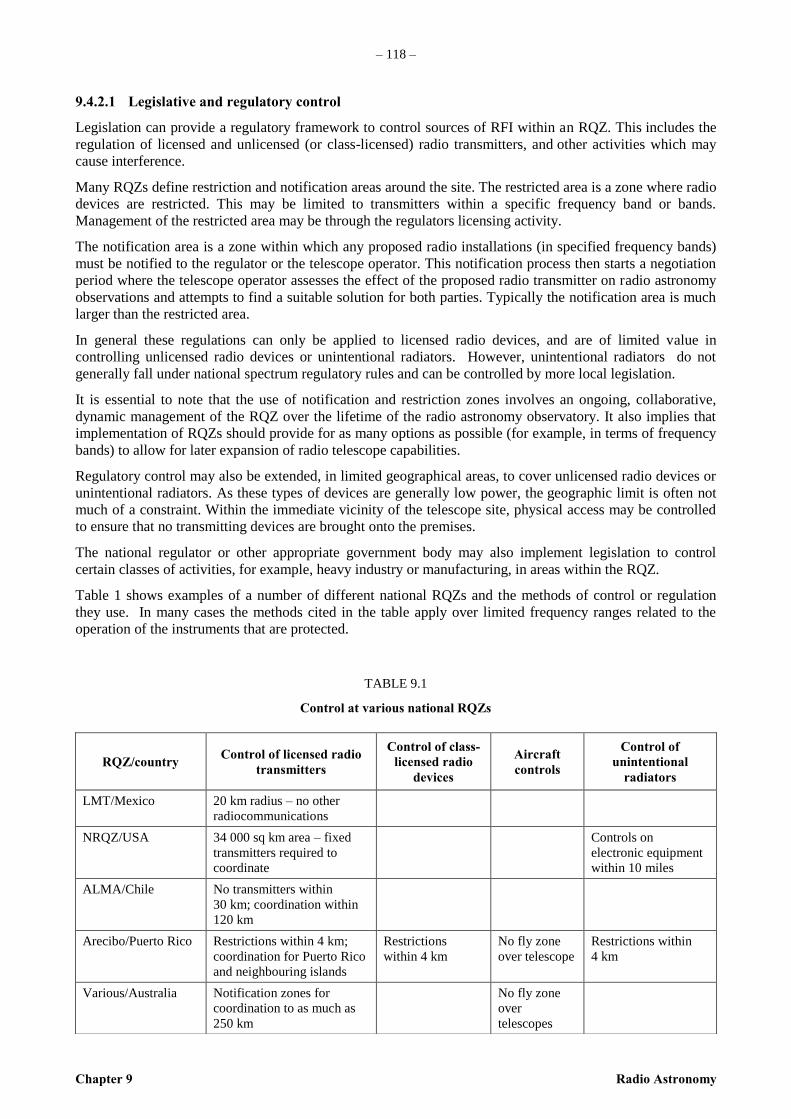
– 118 –
Chapter 9 Radio Astronomy
9.4.2.1 Legislative and regulatory control
Legislation can provide a regulatory framework to control sources of RFI within an RQZ. This includes the
regulation of licensed and unlicensed (or class-licensed) radio transmitters, and other activities which may
cause interference.
Many RQZs define restriction and notification areas around the site. The restricted area is a zone where radio
devices are restricted. This may be limited to transmitters within a specific frequency band or bands.
Management of the restricted area may be through the regulators licensing activity.
The notification area is a zone within which any proposed radio installations (in specified frequency bands)
must be notified to the regulator or the telescope operator. This notification process then starts a negotiation
period where the telescope operator assesses the effect of the proposed radio transmitter on radio astronomy
observations and attempts to find a suitable solution for both parties. Typically the notification area is much
larger than the restricted area.
In general these regulations can only be applied to licensed radio devices, and are of limited value in
controlling unlicensed radio devices or unintentional radiators. However, unintentional radiators do not
generally fall under national spectrum regulatory rules and can be controlled by more local legislation.
It is essential to note that the use of notification and restriction zones involves an ongoing, collaborative,
dynamic management of the RQZ over the lifetime of the radio astronomy observatory. It also implies that
implementation of RQZs should provide for as many options as possible (for example, in terms of frequency
bands) to allow for later expansion of radio telescope capabilities.
Regulatory control may also be extended, in limited geographical areas, to cover unlicensed radio devices or
unintentional radiators. As these types of devices are generally low power, the geographic limit is often not
much of a constraint. Within the immediate vicinity of the telescope site, physical access may be controlled
to ensure that no transmitting devices are brought onto the premises.
The national regulator or other appropriate government body may also implement legislation to control
certain classes of activities, for example, heavy industry or manufacturing, in areas within the RQZ.
Table 1 shows examples of a number of different national RQZs and the methods of control or regulation
they use. In many cases the methods cited in the table apply over limited frequency ranges related to the
operation of the instruments that are protected.
TABLE 9.1
Control at various national RQZs
RQZ/country Control of licensed radio
transmitters
Control of class-
licensed radio
devices
Aircraft
controls
Control of
unintentional
radiators
LMT/Mexico 20 km radius – no other
radiocommunications
NRQZ/USA 34 000 sq km area – fixed
transmitters required to
coordinate
Controls on
electronic equipment
within 10 miles
ALMA/Chile No transmitters within
30 km; coordination within
120 km
Arecibo/Puerto Rico Restrictions within 4 km;
coordination for Puerto Rico
and neighbouring islands
Restrictions
within 4 km
No fly zone
over telescope
Restrictions within
4 km
Various/Australia Notification zones for
coordination to as much as
250 km
No fly zone
over
telescopes

- 119 -
Radio Astronomy Chapter 9
– 1
19 –
9.4.2.2 Alternative technologies and network design
The national regulator or the telescope operator may choose to provide alternative technologies to those
which cause harmful levels of interference. For example, the provision of cable television over fibre-optic
cable may be a suitable replacement for broadcasting. One mobile radio network could be replaced by
another at a more convenient frequency band.
9.5 Implications in establishing an RQZ
9.5.1 Maintenance of RQZs
RQZs require considerable effort to maintain after their creation. Almost the entire burden falls upon the
operator of the radio astronomy facility.
One activity that must be supported is routine monitoring of the radio environment, including all equipment
that is to be installed on the site. This activity is often conducted with standalone monitoring stations and test
facilities that are typically separate from the radio telescope itself.
Another activity is identifying sources of RFI that appear in telescope data, but that might not be sufficiently
strong to detect with the monitoring station(s). Analysis of these cases can be very difficult as the bandwidth,
Doppler tracking, integration time and antenna pattern of a telescope may not be suitable to identify the exact
frequency, time variability or location of the interference source. Moreover, some interference only
becomes apparent long after the observations were taken, when the complete dataset can be fully treated for
the first time. In any case, once RFI has been identified, action must be taken to mitigate or eliminate the
source of the RFI.
RQZ/country Control of licensed radio
transmitters
Control of class-
licensed radio
devices
Aircraft
controls
Control of
unintentional
radiators
MRO/Australia Frequency band plan – RAS
is primary within 70 km;
coordination zone to 260 km
Class licences –
no interference
allowed within
70 km
No fly zone
over site
Protocol for
electronic equipment
used by RAS within
10 km
IRAM/Spain Restrictions on transmitters
up to 5 km radius;
coordination to 10 km radius
1 km minimum
separation to
industry, rail, HV
power lines
Itapetinga/Brazil 4 km diameter zone with no
new urban activity
4 km diameter
zone with no new
urban activity
4 km diameter zone
with no new urban
activity
AGAA/South Africa No transmissions in area of
140 km2, essential services
only in area of up to
123 408 km2
Core area of
140 km2
controlled to
18 500 m
altitude
Pushchino/Russian
Federation
2 km diameter zone with no
new urban activity
Control within
5 km zone
(Pushchino town)
Control the level of
attended interferences
Dominion
RAO/Canada
Licensing tightly controlled
out to 200 km
Nothing within
line-of-sight and
restrictions within
4 km, whichever
is the larger
There was a
no-fly zone
but that has
now expired
No new urban
activity within line of
sight, and restricted
out to 4 km,
whichever is the
larger
FAST/China No transmitters within 5 km;
coordination within 75 km
radius
– 120 –
Chapter 9 Radio Astronomy
Most observatories establish RFI buffer zones within the observatory grounds, with increasingly stringent
restrictions on potentially RFI-generating equipment as distance to the radio astronomy equipment decreases.
Radio quiet zone staff must educate staff and visitors, and be prepared to enforce the local rules.
Considerations for RFI zones should ideally be in place before the observatory is even built.
Radio quiet zone staff will also need to address cases of RFI that arise from sources beyond the observatory
grounds. Unauthorized transmitters that otherwise require an operating license may be the easiest situation to
deal with under national regulation. The most difficult case that arises in RQZ administration is RFI from
unlicensed devices that are external to the observatory property. Dealing with these situations within existing
quiet zones is becoming increasingly problematic. No clear solution is at hand.
A substantial burden in large RQZs can be the processing of license applications for new transmitters within
the quiet zone. Some quiet zones may be easy to administer, if transmitters are simply not allowed within the
quiet zone. Other quiet zones may establish detrimental interference thresholds, in which case license
proposals must be carefully analysed to see if the transmitted signal will exceed established interference
thresholds at the observatory.
Lastly, observatories should not underestimate the need for education and public outreach to explain the need
for the quiet zone, and to make spectrum users aware of their obligations under quiet zone rules.
9.5.2 Long–term considerations
RQZs have often been designed with particular telescopes in mind. The most usual subsequent evolution of
the telescope has then been to increase its utility for higher frequencies through an upgrading of the
instrument. More recently a trend has emerged towards collocation of telescopes onto sites where their
purposes can be adequately met, while they share in the economies of installed infrastructure and regulation,
as well as to shared access to power, communications and roads.
This in turn may well be accompanied by an increase in the frequency range to be protected for the
instruments on a site. It is accordingly advisable to design the parameters of an RQZ as broadly as
circumstances will allow.
Once an RQZ is agreed to, it is required to be in place for a considerable time. This suggests that its
economic impact and its potential impact on future population distribution and development in the affected
area be taken thoroughly into account when designing an RQZ.
Finally, the pace of technical development in society must be expected to continue to result in new
innovations leading to changes in the EMC environment around an RQZ. While impossible to predict, this
trend again indicates the need to design the RQZ to be as broad and robust as possible.
- 121 -
Radio Astronomy Chapter 10
– 1
21 –
CHAPTER 10
Searches for extraterrestrial intelligence (Seti) using observations
at radio frequencies
10.1 Introduction
Fundamental to the perception of our place in the universe is to know whether Earth is the only planet
supporting intelligent life. If the Earth’s intelligent life is truly alone, then it must be either an extraordinary
occurrence or a unique consequence of evolution of the cosmos. On the other hand, if it is but one of a
multitude of intelligent groups populating our Galaxy, then life on Earth may be part of a collection of great
evolutionary diversity, and possibly not unique in its development and civilization. The problem is to
determine whether or not life on Earth is alone.
Some scientists believe that life is common in our Galaxy, and that it could have developed into advanced
forms that possess a telecommunication capability similar or superior to ours. Of course, the details of
transmitting stations – such as the frequencies, modulations, polarisations and locations – used by
extraterrestrial civilizations, if they exist, are not known. To seek the signals from these stations, scientists
must probe the Universe with the most sensitive receiving equipment, carefully and extensively searching the
radio spectrum for tell-tale signs of signals produced by other civilizations.
The first scheme to beam radio signals into space dates back to Tesla’s work in 1899. A special 1939
transmission of signals encoding US television shows has by now reached at least a thousand stars. The most
ambitious attempt to provide other possible civilizations with details about life on Earth occurred in 1974,
with a transmission, sent from the 305 m diameter radio telescope in Arecibo, Puerto Rico, describing our
solar system, DNA composition, and our species.
Morrison and Cocconi [1959] were the first to point out the possibility of receiving radio signals from
extraterrestrial civilizations. Drake [1961] carried out the first microwave search (Project Ozma), using a 25
m radio telescope for observations of two stars about twelve light years away. Since then, scientists from
several countries have conducted more than 99 different documented searches [Tarter, 2001]. Russian
scientists dominated the field for the first decade. The first Russian book in which the SETI problems were
considered was written by I.S. Shklovsky in 1962. The book was translated into many languages and had
great influence on the development of SETI work in the USSR (nowadays Russian Federation). Kardashev
[1963] suggested the possibility of finding more advanced societies than ours, which would have mastered
the technique of radio communication and be capable of producing an output power of more than 1026
W for
transmitting continuous isotropic broadband signals. Many investigations have been carried out [Troitsky et
al., 1971]. Advances in computer and communications technology have made more sensitive and
comprehensive searches possible. Some of the efforts yielded events which could not be explained, for
example, several intriguing signals recorded between 1986 and 1989 during the Megachannel Extraterrestrial
Assay (META) program using a radio telescope at Harvard University, United States of America [Sagan and
Horowitz, 1993]. Recent repetition of observations with much better sensitivity [Lazio et al., 2002] argues
against these being a class of extraterrestrial technological signals. There is, at present, no convincing
evidence of signals from extraterrestrial civilizations. For most of this period, the searches were made with
inadequate sensitivities, and covered only a tiny fraction of the possible frequencies, modulation schemes,
and directions.
Additional background information concerning SETI has been provided by Oliver [1987], Bates [1988], and
Drake and Sobel [1992]. With the advent of relatively inexpensive computer and digital signal processing
technology in the last two decades, more comprehensive searches began. In 1992 NASA launched the
High-Resolution Microwave Survey (HRMS), involving some of the largest radio telescopes on Earth, and
new sensitive radio-receiver equipment. Although the NASA project was cancelled in 1993, the US SETI
Institute continued the high-sensitivity “Targeted Search” portion of the HRMS as Project Phoenix.
– 122 –
Chapter 10 Radio Astronomy
The SETI Institute and the University of California, Berkeley have built the Allen Telescope Array (ATA),
with continuous SETI observations as a major motivation. The ATA has a collecting area equivalent to a 40
m dish. The array has a system noise temperature of 40 K and bandwidth covering the entire range from 0.5
GHz to 11.4 GHz. It generates multiple beams within a field of view (at 1 GHz) allowing full-time SETI
and other radio astronomy observations. The fully-steerable ATA allows longer integration times than were
used in past SETI observations. Advances in computer and digital signal processing technology can also
improve the intrinsic sensitivity of SETI receiver systems.
The ATA also serves as a prototype for a much larger telescope, the square kilometre array (SKA). Now in
the design and prototype phase, the SKA is under development by an international consortium of universities
and research institutes. If international funding is obtained, the SKA will have a collecting area 45 dB greater
than the ATA and more than 13 dB greater than the Arecibo 305 m telescope. Most of the designs under
consideration can form multiple beams thus allowing the possibility of full time SETI observations. Coupled
with more powerful signal processing systems, the SKA will allow a search for the equivalent of terrestrial
radio technology out to 1 000 light years.
The possibility of detecting any microwave signals depends strongly on having a quiet radio environment at
sites where the searches are conducted. Therefore, these sites should be protected to the maximum extent
possible from man-made radio interference. Although modern technology can provide some discrimination
against man-made signals, it may turn out to be inadequate in the face of the rapidly increasing use of the
radio spectrum for a wide variety of telecommunication services and functions. As time passes, the
probability of successful detection would then be correspondingly reduced.
10.2 Detectability of SETI signals
If we assume that signals from extraterrestrial civilizations are reaching the Earth, our ability to detect them
depends upon several factors:
– the strength of the signals arriving at Earth;
– the collecting area and illumination efficiency of the search antenna;
– the sensitivity and frequency flexibility of the receiving system;
– the ability to point the antenna in the direction of the signals;
– the ability to distinguish the received signal from noise due to components of the receiving system,
natural phenomena in the Galaxy, and man-made interference.
Antenna pointing strategies and the selection of search integration time and other system parameters are
important elements of the design of a SETI search. Efforts are being made to develop sensitive systems
covering a broad frequency range and capable of targeting multiple stars simultaneously, surveying the sky
(particularly the Galactic plane), and imaging 2 steradians at once. The eventual performance of these new
systems will be determined to a large extent by the interference environment.
10.3 Signal intensity
The intensity of an extraterrestrial signal at the surface of the Earth depends on the transmitted power and the
characteristics of the path of propagation. The flux density of the signal to be detected is unknown. However,
the distance over which the signal has had to travel must be great, and the intensity at the Earth is expected to
be very low. Detection would therefore be limited by the overall sensitivity of the observing system. Figure
10.1 shows, for several assumed distances of the transmitter, the pfd of the signal received at Earth as a
function of the transmitter power.
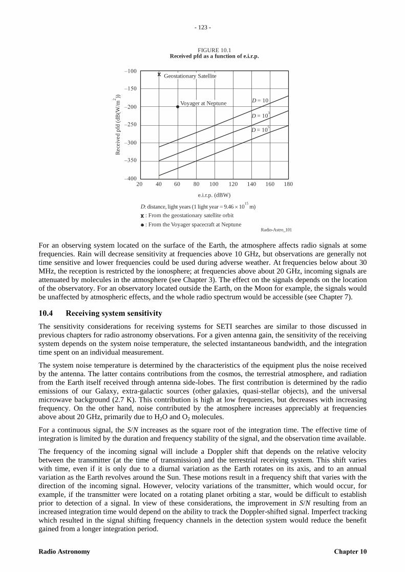
- 123 -
Radio Astronomy Chapter 10
– 1
23 –
Radio-Astro_101
FIGURE 10.1Received pfd as a function of e.i.r.p.
e.i.r.p. (dBW)
Geostationary Satellite
Voyager at Neptune
Rece
ived p
fd (
dB
(W/m
))2
D: distance, light years (1 light year = 9.46 10 m)15
: From the geostationary satellite orbit
: From the Voyager spacecraft at Neptune
D = 10
D = 103
D = 105
20 40 60 80 100 120 140 160 180
–100
–150
–200
–250
–300
–350
–400
For an observing system located on the surface of the Earth, the atmosphere affects radio signals at some
frequencies. Rain will decrease sensitivity at frequencies above 10 GHz, but observations are generally not
time sensitive and lower frequencies could be used during adverse weather. At frequencies below about 30
MHz, the reception is restricted by the ionosphere; at frequencies above about 20 GHz, incoming signals are
attenuated by molecules in the atmosphere (see Chapter 3). The effect on the signals depends on the location
of the observatory. For an observatory located outside the Earth, on the Moon for example, the signals would
be unaffected by atmospheric effects, and the whole radio spectrum would be accessible (see Chapter 7).
10.4 Receiving system sensitivity
The sensitivity considerations for receiving systems for SETI searches are similar to those discussed in
previous chapters for radio astronomy observations. For a given antenna gain, the sensitivity of the receiving
system depends on the system noise temperature, the selected instantaneous bandwidth, and the integration
time spent on an individual measurement.
The system noise temperature is determined by the characteristics of the equipment plus the noise received
by the antenna. The latter contains contributions from the cosmos, the terrestrial atmosphere, and radiation
from the Earth itself received through antenna side-lobes. The first contribution is determined by the radio
emissions of our Galaxy, extra-galactic sources (other galaxies, quasi-stellar objects), and the universal
microwave background (2.7 K). This contribution is high at low frequencies, but decreases with increasing
frequency. On the other hand, noise contributed by the atmosphere increases appreciably at frequencies
above about 20 GHz, primarily due to H2O and O2 molecules.
For a continuous signal, the S/N increases as the square root of the integration time. The effective time of
integration is limited by the duration and frequency stability of the signal, and the observation time available.
The frequency of the incoming signal will include a Doppler shift that depends on the relative velocity
between the transmitter (at the time of transmission) and the terrestrial receiving system. This shift varies
with time, even if it is only due to a diurnal variation as the Earth rotates on its axis, and to an annual
variation as the Earth revolves around the Sun. These motions result in a frequency shift that varies with the
direction of the incoming signal. However, velocity variations of the transmitter, which would occur, for
example, if the transmitter were located on a rotating planet orbiting a star, would be difficult to establish
prior to detection of a signal. In view of these considerations, the improvement in S/N resulting from an
increased integration time would depend on the ability to track the Doppler-shifted signal. Imperfect tracking
which resulted in the signal shifting frequency channels in the detection system would reduce the benefit
gained from a longer integration period.
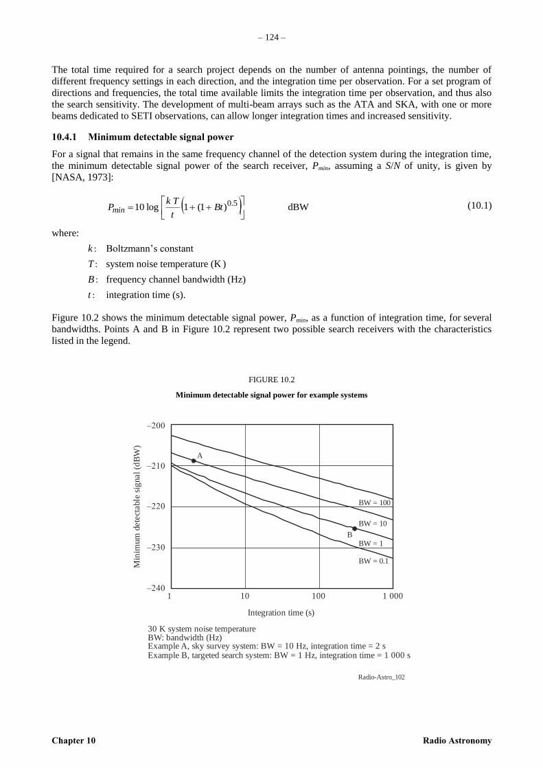
– 124 –
Chapter 10 Radio Astronomy
The total time required for a search project depends on the number of antenna pointings, the number of
different frequency settings in each direction, and the integration time per observation. For a set program of
directions and frequencies, the total time available limits the integration time per observation, and thus also
the search sensitivity. The development of multi-beam arrays such as the ATA and SKA, with one or more
beams dedicated to SETI observations, can allow longer integration times and increased sensitivity.
10.4.1 Minimum detectable signal power
For a signal that remains in the same frequency channel of the detection system during the integration time,
the minimum detectable signal power of the search receiver, Pmin, assuming a S/N of unity, is given by
[NASA, 1973]:
(10.1)
where:
k : Boltzmann’s constant
T : system noise temperature (K )
B : frequency channel bandwidth (Hz)
t : integration time (s).
Figure 10.2 shows the minimum detectable signal power, Pmin, as a function of integration time, for several
bandwidths. Points A and B in Figure 10.2 represent two possible search receivers with the characteristics
listed in the legend.
FIGURE 10.2
Minimum detectable signal power for example systems
Radio-Astro_102
Integration time (s)
Min
imum
dete
ctable
sig
nal
(dB
W)
30 K system noise temperatureBW: bandwidth (Hz)Example A, sky survey system: BW = 10 Hz, integration time = 2 sExample B, targeted search system: BW = 1 Hz, integration time = 1 000 s
BW = 0.1
BW = 100
1 10 100 1 000
–200
–210
–220
–240
–230
BW = 10
BW = 1B
A
dBW)1(1log10 5.0
Bt
t
TkPmin
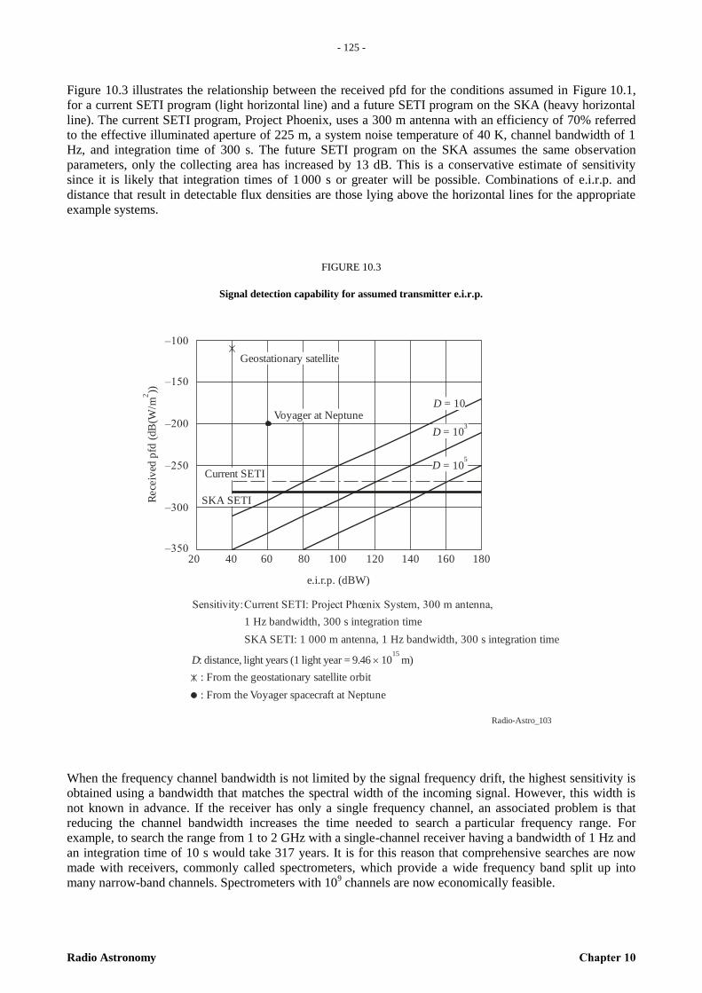
- 125 -
Radio Astronomy Chapter 10
– 1
25 –
Figure 10.3 illustrates the relationship between the received pfd for the conditions assumed in Figure 10.1,
for a current SETI program (light horizontal line) and a future SETI program on the SKA (heavy horizontal
line). The current SETI program, Project Phoenix, uses a 300 m antenna with an efficiency of 70% referred
to the effective illuminated aperture of 225 m, a system noise temperature of 40 K, channel bandwidth of 1
Hz, and integration time of 300 s. The future SETI program on the SKA assumes the same observation
parameters, only the collecting area has increased by 13 dB. This is a conservative estimate of sensitivity
since it is likely that integration times of 1 000 s or greater will be possible. Combinations of e.i.r.p. and
distance that result in detectable flux densities are those lying above the horizontal lines for the appropriate
example systems.
FIGURE 10.3
Signal detection capability for assumed transmitter e.i.r.p.
Radio-Astro_103
e.i.r.p. (dBW)
Geostationary satellite
Voyager at Neptune
Rece
ived
pfd
(dB
(W/m
))2
D: distance, light years (1 light year = 9.46 10 m)15
: From the geostationary satellite orbit
: From the Voyager spacecraft at Neptune
Current SETI
SKA SETI
Sensitivity:Current SETI: Project Phœnix System, 300 m antenna,
1 Hz bandwidth, 300 s integration time
SKA SETI: 1 000 m antenna, 1 Hz bandwidth, 300 s integration time
D = 10
D = 103
D = 105
20 40 60 80 100 120 140 160 180
–100
–150
–200
–350
–250
–300
When the frequency channel bandwidth is not limited by the signal frequency drift, the highest sensitivity is
obtained using a bandwidth that matches the spectral width of the incoming signal. However, this width is
not known in advance. If the receiver has only a single frequency channel, an associated problem is that
reducing the channel bandwidth increases the time needed to search a particular frequency range. For
example, to search the range from 1 to 2 GHz with a single-channel receiver having a bandwidth of 1 Hz and
an integration time of 10 s would take 317 years. It is for this reason that comprehensive searches are now
made with receivers, commonly called spectrometers, which provide a wide frequency band split up into
many narrow-band channels. Spectrometers with 109 channels are now economically feasible.

– 126 –
Chapter 10 Radio Astronomy
10.5 Antenna pointing direction
Antennas with large collecting area (that is, high gain) are desirable in order to increase the search
sensitivity, and correspondingly enhance the probability of detection. However, for single antennas, an
increase in collecting area usually results in a decrease in antenna beamwidth, and the number of position
settings needed to search a given area of sky must be increased. This means that, for a given integration time,
the total search time would need to be increased. Increasing the collecting area by adding additional antennas
could overcome the problem.
The antenna pointing strategy is a fundamental feature of a SETI search. There are two alternatives: targeted
searches, or general sky surveys. In a targeted search, antennas are pointed towards selected stars: there are
nearly a thousand stars similar to the Sun within 100 light years of the Earth. Real-time monitoring of signals
enables a possible detection be checked out on the search antenna or another support instrument. A signal
from an extraterrestrial technology orbiting a target star should vanish when the antenna is directed away
from the target, and return when the target is re-acquired. Because a long time can be spent on each target,
the time-frequency domain of signals output by the spectrometer can be searched for both continuous wave
(CW) and pulsed signals. The search can even extend to patterns drifting in frequency.
Surveys of extra solar planets have provided new targets for SETI searches (Siemion 2013). In addition, the
steadily improving digital signal processing technologies have enabled much broader bandwidth searches,
with finer spectral resolution. The spectral range of a search for narrow band signals (< 5 Hz) towards
detected planets is shown in Figure 10.4.
FIGURE 10.4
Radio background intensity versus frequency plot
Radio-Astro_104
Frequency (GHz)
H O2
No
ise
tem
per
atu
re (
Kel
vin
)
0.1 1 10 1 000
100
10
1100
1 000
O2
O2
H O2
21 cmhyperfine H
21 cmhyperfine OH
Water hole
Terrestrial MicrowaveWindow
Galactic N
on-T
herm
al black
gro
und
GB
T S
ET
I b
an
d
The plot chart shows external contributions to the receiver system temperature and indicates rangesfor SETI. The frequency range 1 to 10 GHz has both low galactic emission and terrestrial
atmosphere contributions to the system temperature. The 0.8 GHz bandwidth Green Bank Telescope Kepler planet search range is shown. Figure from A. Siemion (2013).
Atmospheric rotationaltransitions
General sky surveys over large volumes of space require much more time, and the time spent in each
direction is more limited. Specific scan strategies can be devised to discriminate between signals associated
with celestial objects and signals associated with orbiting or ground-based transmitters.

- 127 -
Radio Astronomy Chapter 10
– 1
27 –
A hybrid of these two concepts is an omni-directional system that uses many small elements for its collecting
area, and combines their outputs to target all possible beams on the visible sky simultaneously. This radio
array will have limited sensitivity unless the number of elements is very large, and that imposes enormous
computing challenges that have not yet become affordable.
10.6 Signal identification and interference rejection
Most searchers assume that the signals from an extraterrestrial civilization will be narrow-band, e.g., 1 Hz,
and possibly may vary in intensity with time. A fundamental problem facing the detection of such signals is
being able to determine that the signal is not the result of natural or man-made noise.
For natural random noise, the probabilities related to amplitude are well understood. The probability that a
noise peak exceeds a search signal threshold may be finite, yet this peak would be registered as a possible
extraterrestrial detection. The rate of these false detections would depend on the adopted threshold level, and
can be calculated for the case of Gaussian (white) noise. Raising the threshold to reduce the rate of false
alarms reduces the receiver sensitivity. Several antennas working in unison lessen the false detection rate.
When these antennas are separated by large distances, terrestrial interference decorrelates and is strongly
reduced.
Man-made signals occupy much of the radio spectrum, particularly at the lower frequencies.
Search strategies should include the ability to classify these signals, and reject them as possible candidates.
The rejection may be based on a-priori knowledge of signals likely to affect an observatory, or on
measurements made at the observatory. The success in excluding these interfering signals from the data base
used for further detailed analysis is a major component in the feasibility of a successful search.
The increasing use of the radio spectrum by radiocommunication and other services will make future SETI
searches more difficult. In particular, the rapidly growing addition of satellites to the geostationary orbit will
increasingly preclude the possibility of searching a zone of sky in directions close to the orbit at many
frequencies. It should be noted that, from the point of view of SETI, all man-made radio emissions, whether
authorized or not, represent potential radio frequency interference. In view of the increasing demands on the
radio spectrum, it is clear that SETI searches should be conducted as soon as possible to minimize the
problem of radio interference.
10.7 Candidate bands to be searched
There can be no prior knowledge of the frequency and other characteristics of signals that may be detected
from extraterrestrial civilizations, and one cannot realistically cover the entire radio spectrum, or even that
part which is available to observatories on the Earth’s surface. Therefore, restricted frequency bands must be
selected on the basis of calculated guesses.
Ex-CCIR Report 700-1 (Dusseldorf, 1990) discusses the rationale for the selection of particular frequency
bands for the searches. A common aspect of many of the suggested bands is an association with frequencies
of naturally occurring phenomena. The underlying assumption is that extraterrestrial civilizations may elect
to transmit at frequencies that are common throughout the Galaxy, or are at some multiple of these common
frequencies, on the basis that other civilizations would be also aware of these frequencies and would plan
their receiving systems accordingly. Thus, the bands are related to frequencies of known spectral lines
associated with the most abundant interstellar atoms and molecules atomic hydrogen (HI) at 1 420 MHz,
hydroxyl radical (OH) at 1 612, 1 665, 1 667 and 1 720 MHz, and formaldehyde (H2CO) at 4 830 MHz. The
region between the hydrogen and hydroxyl lines, called the “water hole”, has been favoured in the belief that
water-based life forms might consider this spectral region significant. A band containing a 203 GHz spectral
line of the lightest artificial atom, positronium, has even been suggested.
Several bands allocated to the RAS are protected from man-made emissions, as are also several bands
allocated for passive sensing. Because they are protected from interference, and in many cases contain
spectral lines occurring widely throughout the Galaxy, these bands are good candidates for use in a SETI
programme.
There are many points of view concerning choice of bands. However, because there is no a priori knowledge
about the character or even existence of the extraterrestrial signals, comprehensive searches should cover a
frequency range as wide as possible.
– 128 –
Chapter 10 Radio Astronomy
REFERENCES
BATES, D. [1988] Radio searches for extraterrestrial civilizations. Quarterly J. of the Royal Astronom. Soc.,
Vol. 29, p. 307-311.
COCCONI, G. and MORRISON, P. [1959] Searching for interstellar communications. Nature, 184,
p. 844-846.
DRAKE, F. D. [1961] Project Ozma. Physics Today, Vol. 14, p. 40-46.
DRAKE, F. D. and SOBEL, D. [1992] Is anyone out there?: The Scientific Search for Extraterrestrial
Intelligence. Delacorte Press, New York, United States of America.
KARDASHEV, N. S. [1964] Transmission of Information by Extraterrestrial Civilizations. Soviet
Astronomy, AJ, 8, p. 217-221.
LAZIO, T. J. W., TARTER, J. C. and BACKUS, P. R. [July 2002] The META Candidates Were Not
Transmissions From Intrinsically Steady Sources. Astronomical J., Vol. 124, p. 560-564.
NASA [July 1973] Project Cyclops. Ames Research Center, Moffett Field, California, United States of
America, Report CR 114445, Revised Edition, p. 243.
OLIVER, B. M. [1987] The windows of SETI: frequency and time in the search for extraterrestrial
intelligence. The Planetary Report, Vol. VII, 6, p. 23-25.
SAGAN, C. and HOROWITZ, P. [September 1993] Five Years Of Project META: An All-Sky Narrowband
Radio Search For Extraterrestrial Signals. Astrophysical J., Vol. 415, 218, p. 218-235.
TARTER, J. C. [2001] The Search for Extraterrestrial Intelligence (SETI). Annual Rev. of Astronom. and
Astrophys., Vol. 39, p. 511-548.
TROITSKY, V. S., STARODUBTSEV, A. M., GERSHTEIN, L. L and RAKHLIN, V. L. [1971]
The experience of the search for monochromatic radio emission from stars in the vicinity of the Sun at a
frequency of 927 mc/s. Astronomicheskii Zhurnal, Vol. 48, p. 645-647.
SIEMION, A. P. V, DEMOREST, P., KORPELA, E. MADDALENA, R., WERTHIMER, D., COBB, J.,
HOWARD, A.W.,LANGSTON, G., LEBOFSKY, M, MARCY, G.W., TARTER, J., A 1.1-1.9 GHz SETI
Survey of the Kepler Field. I. A Search for Narrow-band Emission from Select Targets, Astrophysical. J.,
Vol. 767, p. 94.
SHKLOVSKII, I. S. and SAGAN, C. [1966] Intelligent life in the Universe, Holden-Day, Inc.
- 129 -
Radio Astronomy Chapter 11
– 1
29 –
CHAPTER 11
Ground-based radar astronomy
11.1 Introduction
Radar astronomy has the same requirements as radio astronomy, namely access to interference-free bands in
the radio spectrum. It differs from radio astronomy in that it is an active service, transmitting as well as
receiving. It also differs in that there are only three transmitting sites currently active in the field, one in
Puerto Rico, one in California, and one in the Crimea, operating in four bands between 430 MHz and 8 GHz
(see Table 11.1). Since the reception of a radar echo can be either by the transmitting antenna or by an
auxiliary antenna, there are approximately twice as many active receiving sites as transmitting sites. All of
the transmitting and receiving antennas currently in use are also used for passive radio astronomy
observations or for spacecraft communications. There has been a renewal of interest in radar observations of
the solar corona and discussions of a transmitter system to operate in conjunction with the planned low
frequency array radio telescope (LOFAR). A frequency has not been selected but it would probably be in the
range 15 MHz to 50 MHz.
Radar astronomy involves the use of Earth-based radar systems to:
– study the radio wavelength reflection properties, size and rotation vectors of the large and small
solid bodies in the solar system;
– measure Doppler shifts and time delays to derive velocities and distances for determination of
orbital parameters, especially for near Earth asteroids which may pose a future threat to the Earth;
– study the interplanetary medium and solar corona via their effects on radar signals propagating
through them and by studying radar reflections from the solar corona.
Related disciplines which have similar requirements to radar astronomy are the studies of the Earth’s
ionosphere and atmosphere using incoherent scatter, stratospheric and meteor radars.
Radar astronomy had its official beginning in 1946 with the detection of the first echoes from the Moon, but
its real start as a sub-discipline of astronomy was in 1961 with the detection of echoes from Venus. Detection
of the other terrestrial planets, Mercury and Mars, followed soon after. The successes of these early years
included the determination of the rotation periods of Venus and Mercury and a factor of one hundred
improvement in our knowledge of the astronomical unit. These years also saw considerable emphasis on the
development of observational techniques and instrumentation. A description of the early observations and
instrumentation development can be found in Evans and Hagfors [1968] and an account of the early history
of radar astronomy can be found in Butrica [1996].
The second decade of radar astronomy beginning in the early 1970s saw a considerable increase in the
sensitivity of the systems used, with the installation of a 2.38 GHz radar on the then newly resurfaced 305 m
Arecibo telescope, and improvements to the 8.5 GHz system on the then NASA/JPL Goldstone 64 m
telescope. At the same time, the UK Jodrell Bank and US Haystack planetary radar systems ceased
operations, leaving two antennas in the United States of America and one in the then Soviet Union (now the
Republic of the Ukraine) as the only planetary radar astronomy transmitting sites; this situation persists to
this day, as indicated in Table 11.1.
– 130 –
Chapter 11 Radio Astronomy
In the twenty years between 1972 and 1992, radar astronomy made many contributions to our knowledge of
the solar system (see Ostro [2002] for a review). The particles in the rings of Saturn were found to be
centimetre-sized or larger, the unusual scattering properties of the icy Galilean satellites of Jupiter were
discovered, 40% of the surface of Venus was imaged at 2 km resolution, ice deposits were discovered at the
poles of Mercury, the radio wavelength reflection properties were measured for dozens of main belt and
near-Earth asteroids plus several comets, and high-resolution delay-Doppler images were obtained for two
Earth-approaching asteroids. In the area of instrumentation, radar interferometry was introduced to resolve
the north-south ambiguity inherent in delay-Doppler imaging, bistatic systems were developed, especially
between the Goldstone antenna (transmitting) and the VLA in New Mexico (receiving), and pseudo-infinite
length coding schemes were used to overcome the overspread problem when imaging rapidly rotating
targets.
During the mid-1990s the optics of the Arecibo telescope were changed to use a dual Gregorian sub-reflector
system to correct for the telescope’s spherical aberration. A 15 m high ground screen was also constructed
around the perimeter of the 305 m primary reflector to shield the receivers from ground radiation. These
modifications resulted in a significant increase in the sensitivity of the telescope at frequencies above 1.0
GHz and a reduction in system temperatures. When combined with a doubling of the power of the S-Band
transmitter to 1 MW, these improvements resulted in an increase in the sensitivity of the Arecibo S-Band
radar system of a factor of 10 at zenith and over a factor of 20 at the telescope’s maximum zenith angle of
20. At about the same time improved klystrons gave a small improvement in the sensitivity of the Goldstone
X-Band radar system. The Goldstone S-Band planetary radar transmitter was decommissioned in 2001.
Over the past few years the upgraded Arecibo and Goldstone systems have been used extensively for studies
of both near Earth (NEAs) and mainbelt asteroids resulting in the discovery of binary NEAs. Arecibo has
been used to study the surfaces of Titan and Iapetus, satellites of Saturn, and to image the rings of Saturn.
Higher resolution imagery has been obtained for the ice deposits at the poles of Mercury, altimetric
observations have been made of the polar regions of the Moon and surficial deposits on the surface of Venus
studied via an analysis of the polarisation properties of the reflected echo.
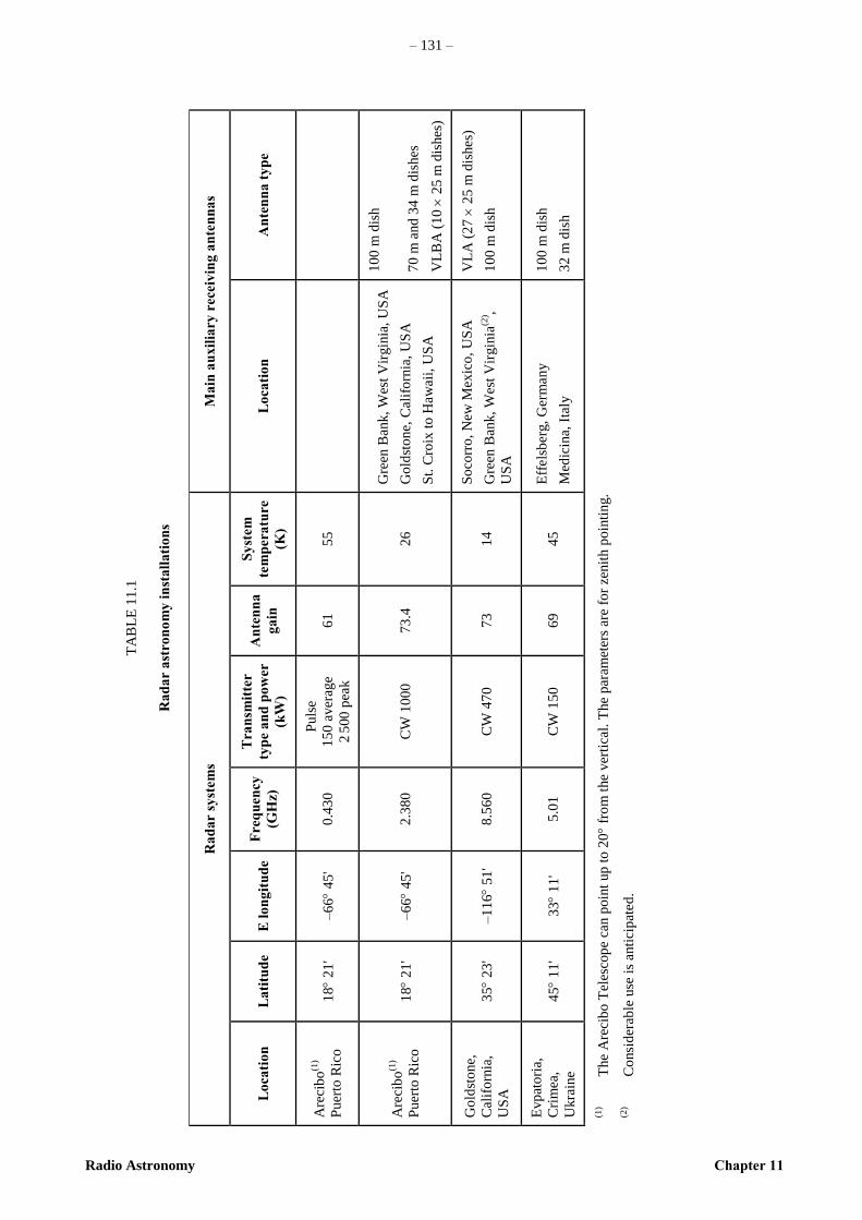
– 131 –
Radio Astronomy Chapter 11
TA
BL
E 1
1.1
Ra
da
r a
stro
no
my
in
sta
lla
tio
ns
Ra
da
r sy
stem
s M
ain
au
xil
iary
rece
ivin
g a
nte
nn
as
Lo
cati
on
L
ati
tud
e
E l
on
git
ud
e
Fre
qu
ency
(GH
z)
Tra
nsm
itte
r
typ
e a
nd
po
wer
(kW
)
An
ten
na
ga
in
Sy
stem
tem
per
atu
re
(K)
Lo
cati
on
A
nte
nn
a t
yp
e
Are
cib
o(1
)
Puer
to R
ico
1
8
21
' –
66
45
' 0
.43
0
Puls
e
15
0 a
ver
age
2 5
00
pea
k
61
55
Are
cib
o(1
)
Puer
to R
ico
1
8
21
' –
66
45
' 2
.38
0
CW
10
00
73
.4
26
Gre
en B
ank,
Wes
t V
irgin
ia,
US
A
Go
ldst
one,
Cal
ifo
rnia
, U
SA
St.
Cro
ix t
o H
aw
aii,
US
A
10
0 m
dis
h
70
m a
nd
34
m d
ishes
VL
BA
(1
0
25 m
dis
hes
)
Go
ldst
one,
Cal
ifo
rnia
,
US
A
35
23
' –
11
6
51
' 8
.56
0
CW
47
0
73
14
So
corr
o,
New
Mex
ico
, U
SA
Gre
en B
ank,
Wes
t V
irgin
ia(2
) ,
US
A
VL
A (
27
2
5 m
dis
hes)
10
0 m
dis
h
Evp
ato
ria,
Cri
mea
,
Ukra
ine
45
11
' 3
3
11
' 5
.01
CW
15
0
69
45
Eff
els
ber
g,
Ger
man
y
Med
icin
a, I
taly
10
0 m
dis
h
32
m d
ish
(1)
The
Are
cib
o T
eles
cop
e ca
n p
oin
t up
to
20
fro
m t
he
ver
tica
l. T
he
par
amet
ers
are
for
zenit
h p
oin
tin
g.
(2)
Co
nsi
der
able
use
is
anti
cip
ated
.
– 132 –
Chapter 11 Radio Astronomy
11.2 Sensitivity issues
To achieve its objectives, the study of the large and small bodies in our solar system, radar astronomy is
driven by the need for large antennas, high-powered transmitters, and very low-noise front-end amplifiers.
This need is dictated by the inverse fourth power dependence of received signal strength with distance. For
an antenna with forward gain, G, equipped with a CW transmitter of power, PT, (with the exception of the
Arecibo 430 MHz system, all planetary radar transmitters are CW since for virtually all objects studied the
overall sensitivity is dependent on the average transmitted power) the power P received by an antenna with
effective collecting area A after reflection from a target with cross section at a distance R from the radar is
given by:
22)( 4 R
AGPP T
(11.1)
If, as is normally the case, the same antenna is used for both transmitting and receiving at wavelength ,
then:
43
22
)(4 R
GPP T
(11.2)
The overall sensitivity of the radar system is dependent on the ratio of the received signal power to the rms
noise power fluctuations arising from additive noise contributions from the sky (the microwave background
and, at the lower frequencies, non-thermal radiation from our Galaxy), the atmosphere, ground radiation, the
front-end amplifiers and, of course, interference. The sum of these noise powers is normally characterized by
a system temperature, Ts, which is related to the noise power, PN, by PN k Ts B, where k is Boltzmann’s
constant and B is the relevant frequency bandwidth, normally the Doppler broadening. The r.m.s. noise
fluctuations are given by PN (B)–1/2
where is the integration time.
Ignoring the target properties and other constants:
Sensitivity 2/1)/( B
T
GAP
S
T (11.3)
or, in the case where the same antenna is used for transmitting and receiving:
Sensitivity 2/1
22
)/( BT
GP
S
T
(11.4)
Thus, the requirements of radar astronomy are very similar to those of radio astronomy (large antennas, low-
noise front-end amplifiers and an absence of interfering signals), coupled with very high-powered
transmitters. Since the gain, G, is inversely proportional to 2, equations (11.1) and (11.2) imply that the
higher the frequency, the higher the sensitivity.
11.3 Operational modes and bandwidth requirements
Both CW and modulated waveforms are used in radar astronomy with the choice depending on the nature of
the target object and the aims of the experiment. In CW experiments where a monochromatic signal is
transmitted, the reflected signal is Doppler broadened due to the target object’s rotational angular velocity
rad/s with the broadening given by:
sin4 0
c
a (11.5)

- 133 -
Radio Astronomy Chapter 11
– 1
33 –
where:
a : object radius
0 : transmitted frequency
c : velocity of light
: angle between the rotation axis and the LoS from the radar.
Normally, a circularly-polarised wave is transmitted, and the spectra of the reflected signal in the two senses
of received circular polarisation provides information about the radar albedo, the wavelength scale surface
roughness, the rotation period, etc. While frequency switching of the transmitted signal every few seconds
may be used to improve detectability of the received signal, the total bandwidths used for transmission and
reception in the CW case rarely exceed a few tens of kilohertz.
Two-dimensional (delay-Doppler) imaging is used to map the radio wavelength reflection properties over the
surfaces of the terrestrial planets, asteroids and, hopefully in the future, comets. The necessary modulation of
the transmitted signal can be achieved by pulse modulation. Some early systems were pulsed but all recent
ones have been CW since sensitivity is normally dependent on the average transmitted power, and high
average powers are more easily and cheaply obtained with CW transmitters. Therefore, modern systems
phase-modulate a CW signal using a bi-phase modulation based on repetitive, maximal-length, shift-register
codes. The properties of the autocorrelation functions of these codes make them ideal for planetary radar
applications. At present, the shortest basic interval in routine use for switching the phase between the two
states 180 apart is 0.1 ms, corresponding to a range resolution of 15 m. The receiver bandwidth needed when
a 0.1 ms switching interval is used is approximately 20 MHz, and this bandwidth sets radar astronomy’s
current requirements. The Doppler shift due to the relative motion of the target object and the Earth can
offset the receiver band relative to the transmitter frequency by up to several megahertz. Of course, strong
interference just outside the edges of this band could cause significant degradation of receiver performance.
11.4 Radar astronomy installations
As an active service with stringent requirements for interference-free bands in the radio spectrum, radar
astronomy has the same requirements as radio astronomy, but without access to protected bands. To date, the
frequencies chosen have been dictated by considerations such as the availability of high-powered klystrons
or, as is the case for the 8.5 GHz Goldstone facility, the need for high-powered transmitters for other
purposes such as spacecraft communications.
Table 11.1 shows the systems currently used for planetary radar astronomy. The two most sensitive are the
8.5 GHz system on the 70 m antenna of NASA Deep Space Network at Goldstone, California, and the 2.4
GHz system on the 305 m Arecibo radio/radar telescope in Puerto Rico, operated by SRI International,
USRA and UMET, under a cooperative agreement with the U.S. National Science Foundation NSF, with
support from NASA for the planetary programme.
– 134 –
Chapter 11 Radio Astronomy
REFERENCES
BUTRICA, A. J. [1996] To See the Unseen: A History of Planetary Radar Astronomy. NASA SP-4218,
NASA History Office.
EVANS, J. V. and HAGFORS, T., Ed. [1968] Radar Astronomy, McGraw-Hill.
OSTRO S. J. [2002] Planetary radar astronomy. Encyclopedia of Physical Science and Technology,
Third Edition, Vol. 12, p. 295-327, Academic Press.
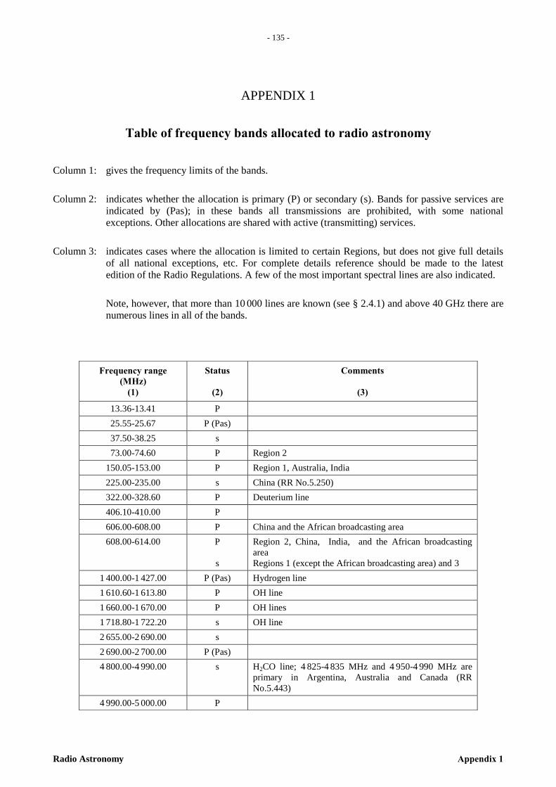
- 135 -
Radio Astronomy Appendix 1
– 1
35 –
APPENDIX 1
Table of frequency bands allocated to radio astronomy
Column 1: gives the frequency limits of the bands.
Column 2: indicates whether the allocation is primary (P) or secondary (s). Bands for passive services are
indicated by (Pas); in these bands all transmissions are prohibited, with some national
exceptions. Other allocations are shared with active (transmitting) services.
Column 3: indicates cases where the allocation is limited to certain Regions, but does not give full details
of all national exceptions, etc. For complete details reference should be made to the latest
edition of the Radio Regulations. A few of the most important spectral lines are also indicated.
Note, however, that more than 10 000 lines are known (see § 2.4.1) and above 40 GHz there are
numerous lines in all of the bands.
Frequency range
(MHz)
(1)
Status
(2)
Comments
(3)
13.36-13.41 P
25.55-25.67 P (Pas)
37.50-38.25 s
73.00-74.60 P Region 2
150.05-153.00 P Region 1, Australia, India
225.00-235.00 s China (RR No.5.250)
322.00-328.60 P Deuterium line
406.10-410.00 P
606.00-608.00 P China and the African broadcasting area
608.00-614.00 P
s
Region 2, China, India, and the African broadcasting
area
Regions 1 (except the African broadcasting area) and 3
1 400.00-1 427.00 P (Pas) Hydrogen line
1 610.60-1 613.80 P OH line
1 660.00-1 670.00 P OH lines
1 718.80-1 722.20 s OH line
2 655.00-2 690.00 s
2 690.00-2 700.00 P (Pas)
4 800.00-4 990.00 s H2CO line; 4 825-4 835 MHz and 4 950-4 990 MHz are
primary in Argentina, Australia and Canada (RR
No.5.443)
4 990.00-5 000.00 P
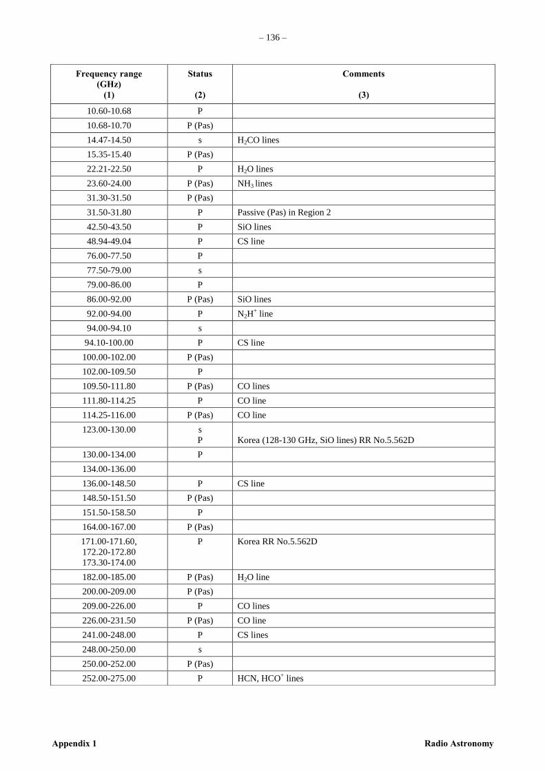
– 136 –
Appendix 1 Radio Astronomy
Frequency range
(GHz)
(1)
Status
(2)
Comments
(3)
10.60-10.68 P
10.68-10.70 P (Pas)
14.47-14.50 s H2CO lines
15.35-15.40 P (Pas)
22.21-22.50 P H2O lines
23.60-24.00 P (Pas) NH3 lines
31.30-31.50 P (Pas)
31.50-31.80 P Passive (Pas) in Region 2
42.50-43.50 P SiO lines
48.94-49.04 P CS line
76.00-77.50 P
77.50-79.00 s
79.00-86.00 P
86.00-92.00 P (Pas) SiO lines
92.00-94.00 P N2H+ line
94.00-94.10 s
94.10-100.00 P CS line
100.00-102.00 P (Pas)
102.00-109.50 P
109.50-111.80 P (Pas) CO lines
111.80-114.25 P CO line
114.25-116.00 P (Pas) CO line
123.00-130.00 s
P
Korea (128-130 GHz, SiO lines) RR No.5.562D
130.00-134.00 P
134.00-136.00
136.00-148.50 P CS line
148.50-151.50 P (Pas)
151.50-158.50 P
164.00-167.00 P (Pas)
171.00-171.60,
172.20-172.80
173.30-174.00
P Korea RR No.5.562D
182.00-185.00 P (Pas) H2O line
200.00-209.00 P (Pas)
209.00-226.00 P CO lines
226.00-231.50 P (Pas) CO line
241.00-248.00 P CS lines
248.00-250.00 s
250.00-252.00 P (Pas)
252.00-275.00 P HCN, HCO+ lines
- 137 -
Radio Astronomy Appendix 1
– 1
37 –
In addition to the allocations, RR No. 5.149 urges administrations to take all practicable steps to protect the
RAS from harmful interference in the following bands:
13 360-13 410 kHz,
25 550-25 670 kHz,
37.5-38.25 MHz,
73-74.6 MHz in Regions 1 and 3,
150.05-153 MHz in Region 1,
322-328.6 MHz,
406.1-410 MHz,
608-614 MHz in Regions 1 and 3,
1 330-1 400 MHz,
1 610.6-1 613.8 MHz,
1 660-1 670 MHz,
1 718.8-1 722.2 MHz,
2 655-2 690 MHz,
3 260-3 267 MHz,
3 332-3 339 MHz,
3 345.8-3 352.5 MHz,
4 825-4 835 MHz,
4 950-4 990 MHz,
4 990-5 000 MHz,
6 650-6 675.2 MHz,
10.6-10.68 GHz,
14.47-14.5 GHz,
22.01-22.21 GHz,
22.21-22.5 GHz,
22.81-22.86 GHz,
23.07-23.12 GHz,
31.2-31.3 GHz,
31.5-31.8 GHz in Regions 1 and 3,
36.43-36.5 GHz,
42.5-43.5 GHz,
48.94-49.04 GHz,
76-86 GHz,
92-94 GHz,
94.1-100 GHz,
102-109.5 GHz,
111.8-114.25 GHz,
128.33-128.59 GHz,
129.23-129.49 GHz,
130-134 GHz,
136-148.5 GHz,
151.5-158.5 GHz,
168.59-168.93 GHz,
171.11-171.45 GHz,
172.31-172.65 GHz,
173.52-173.85 GHz,
195.75-196.15 GHz,
209-226 GHz,
241-250 GHz,
252-275 GHz
At frequencies above 275 GHz, there are no ITU-R band allocations. However, WRC-2012 approved
the following provision via RR No. 5.565:
5.565 The following frequency bands in the range 275-1 000 GHz are identified for use by
administrations for passive service applications:
– radio astronomy service: 275-323 GHz, 327-371 GHz, 388-424 GHz, 426-442 GHz,
453-510 GHz, 623-711 GHz, 795-909 GHz and 926-945 GHz;
– Earth exploration-satellite service (passive) and space research service (passive):
275-286 GHz, 296-306 GHz, 313-356 GHz, 361-365 GHz, 369-392 GHz, 397-399 GHz,
409-411 GHz, 416-434 GHz, 439-467 GHz, 477-502 GHz, 523-527 GHz, 538-581 GHz,
611-630 GHz, 634-654 GHz, 657-692 GHz, 713-718 GHz, 729-733 GHz, 750-754 GHz,
771-776 GHz, 823-846 GHz, 850-854 GHz, 857-862 GHz, 866-882 GHz, 905-928 GHz,
951-956 GHz, 968-973 GHz and 985-990 GHz.
The use of the range 275-1 000 GHz by the passive services does not preclude use of this range
by active services. Administrations wishing to make frequencies in the 275-1 000 GHz range available for
active service applications are urged to take all practicable steps to protect these passive services from
harmful interference until the date when the Table of Frequency Allocations is established in the above-
mentioned 275-1 000 GHz frequency range.
All frequencies in the range 1 000-3 000 GHz may be used by both active and passive
services. (WRC-12)
– 138 –
Appendix 2 Radio Astronomy
APPENDIX 2
Registration of radio astronomy stations
It is important for administrations operating radio astronomy stations to register them with the
Radiocommunications Bureau (BR) of the International Telecommunication Union (ITU).
Registration offers a number of advantages:
– Co-channel interference protection, when observations are conducted in shared bands allocated to the
RAS on a primary basis, particularly when cross-border protection is important.
– Several footnotes in the Radio Regulations provide protection to radio astronomy stations from
unwanted emissions by satellites. As an example, footnote RR No. 5.511A states:
“ ... In order to protect the radio astronomy service in the band 15.35-15.4 GHz, the aggregate power
flux-density radiated in the 15.35-15.4 GHz band by all the space stations within any feeder-link of a
non-geostationary system in the mobile-satellite service (space-to-Earth) operating in the 15.43-15.63
GHz band shall not exceed the level of 156 dB(W/m2) in a 50 MHz bandwidth, into any radio
astronomy observatory site for more than 2% of the time.”
When examining a satellite system for compliance with such a footnote, the BR will consider only those
radio astronomy stations that are registered. Registration will:
– allow a radio astronomy station to be taken into account by those planning to establish new
transmitters in its vicinity. International registration is particularly important when a station is located
close to a national border, and bilateral or multilateral coordination may be necessary or desirable;
– establish chronological priority for the registered station. When registered, radio astronomy stations
observing in certain bands (e.g. 15.35-15.4 GHz) may claim protection from unwanted emissions of
satellite systems filed for operation in adjacent or nearby bands at a later date.
Registration of radio astronomy stations must take place through the telecommunications authority of
national administrations. The characteristics of the radio astronomy station that must be supplied are
described in Annex 2, Appendix 4 of the Radio Regulations.
Portions of the RR, including the parameters required for registration of a radio astronomy station may be
modified at every WRC. For example, WRC-03 added several new parameters to those required to register a
radio astronomy station (such as minimum elevation angle at which a radio telescope may observe, which is
necessary to calculate the aggregate power flux-density of space stations in a non-geostationary satellite
system as referred in footnote RR No. 5.511A). The most recent version of the RR should be consulted
before registering a particular station.
Most radio astronomy stations observe over spectrum ranges that are wider than the bands that are allocated
to radio astronomy. In registering radio astronomy stations, care should be taken in breaking up the
observing frequency ranges into those portions that are allocated to radio astronomy on a primary basis and
those that are not, as protection of the station applies only in primary radio astronomy bands. For example, if
a station operates a receiver that covers the range 15-16 GHz, the station should be registered in three
frequency bands:
– 15.00-15.35 GHz where no protection applies;
– 15.35-15.40 GHz where footnote RR No. 5.511A applies, and
– 15.40-16.00 GHz where no protection applies.
If the 15.00-16.00 GHz band is registered as a single entity, no protection will be provided to any portion of
it. Registration of spectrum ranges that do not receive protection could still be useful for purposes of
planning and coordination.
- 139 -
RADIO ASTRONOMY Appendix 3
– 1
39 –
APPENDIX 3
Units in radio astronomy
Radio astronomers use a number of units and specifications that are different from those used in most other
services. The purpose of this appendix is to provide a translation between jargon used by radio astronomers
and that used by other services, particularly with regard to signal strength and antenna gain.
Signal strength
Radio astronomers specify signal strength in units of Janskys (abbreviated Jy). The unit is named for Karl
Jansky, the discoverer of cosmic radio signals. The Jy is a unit of power per unit area per unit bandwidth (i.e.
power spectral flux density):
1 Jy ≡ 10-26
W/(m2 Hz)
Several factors make radio astronomers express signal strength in Jy:
– Radio astronomy signals are very weak, hence the very small value of the Jy.
– Radio astronomers use a variety of different antennas with different collecting area. To be able to
compare measured signal strengths among different antennas, the Jy expresses the signal strength on a
per unit area of antenna collecting surface. By normalizing the per unit area and per unit bandwidth,
the Jy allows measured signal strengths to be directly compared among different radio telescopes.
– Many radio astronomy signals are broadband (for example, thermal emission from a warm gas), and
the power received depends on the total receiver bandwidth. The Jy takes this into account by
expressing the signal strength on a per unit bandwidth basis.
Many radiocommunication services express signal strength in terms of power only. A common unit is the
dBm, or decibels above 1 mW. The dBm is a logarithmic unit, which is useful because of the many orders of
magnitude range in signal strength that can be expressed from terrestrial radio signals, especially given the
dBm can be used to express both transmit and received power, which can range over 200 dB or more. For
comparison, signal strengths in radio astronomy do not vary over quite such a large range – a 1 Jy source is
very strong, and typical radio telescope sensitivities range down to the microjansky (μJy) level, or only about
60 dB total range.
While the Jy (power spectral flux density) and the dBm (power) are two different units, they can be
compared given some nominal assumptions. A Jy is converted to a power by multiplying by the receiver
bandwidth and the effective antenna collecting area. The following table compares the two by assuming a
bandwidth relevant to some common terrestrial signals, and by assuming that the antenna collecting area
corresponds to the isotropic collecting area, λ2/4π:
Power (in mW) = Power Spectral Flux Density (in Jy) * 10-26
W/(m2 Hz) * 1000 mW/W * bandwidth (Hz) *
[Wavelength (m)]2 ÷ 4π
Power (dBm) = 10 * log10[Power (mW)]

– 140 –
Appendix 3 Radio Astronomy
Examples of received signal strength in dBm corresponding to a 1 Jy signal received by an isotropic
antenna across the specified bandwidth, for a number of common signals
To put these numbers in perspective, the reference GSM handset sensitivity is -111 dBm (per the GSM
specifications), therefore a 1 Jy signal is 93 dB below the GSM sensitivity limit, while a 1 μJy signal is some
153 dB below the GSM sensitivity limit. A radio telescope can be more than 15 orders of magnitude more
sensitive than a GSM receiver.
A radio astronomer attempting to convert terrestrial signal strength into its Jy equivalent may occasionally
find signal strengths expressed in microvolts per meter (μV/m), or its decibel equivalent, dB(μV/m)12
. This is
simply a measure of the electric field amplitude (E), and Ohm’s Law can be used to convert E to an
equivalent power: P(W/m2) = E
2/Z0, where Z0 = 377 Ω is the impedance of free space. Electric field
amplitudes (instead of power) are often encountered in EMC work, for example in the U.S. Federal
Communications Commission’s unlicensed devices rules. With a bit of algebra, the following conversions
are derived:
P(mW) = 1.9x10⁻⁸
* [E(μV/m)]2 * [f(MHz)]
-2
P(dBm) = -77.2 + E[dB(μV/m)] – 20*log10[f(MHz)]
This conversion is also noted in Report ITU-R RA.2131 which gives the protection thresholds for RAS
observations in terms of their electric field equivalents
Antennas
Radio astronomers commonly convert power flux density or spectral power flux density (both measures of
power or power spectral density over a unit area) into a total power. The effective collecting area of the
antenna is therefore a more useful expression of antenna performance than antenna gain. The effective
antenna collecting area Ae is a combination of the geometrical collecting area Ag (if defined) and the aperture
efficiency ηa: Ae = ηa Ag. A common expression of radio astronomy antenna gain is the rise in receiver
temperature (in Kelvins) attributable to the collection of power in a single polarisation from a source of total
flux density (F) of 1 Jy. This is referred to as the antenna gain (G) in K/Jy. To convert between Ae and G:
( )
where kB is Boltzmann’s constant.
Radiocommunication services typically specify basic antenna performance by a different expression of
antenna gain: The amount by which the signal strength at the output of an antenna is increased (or decreased)
relative to the signal strength that would be obtained at the output of a standard reference antenna, assuming
the signal was along the main beam of the reference antenna. The most common reference antenna is the
isotropic antenna. The effective collecting area Ae of an isotropic antenna is λ2/4π = 7162/[f(MHz)]
2,
____________________
12 Note that dB(μV/m) = 20*log10(μV/m), and not 10* log10(μV/m), because it is an electric field value rather than a power value.
Signal type Bandwidth Frequency/Wavelength dBm corresponding to 1 Jy
Land mobile 12.5 kHz 450 MHz/0.67 m 1 Jy = -204 dBm
GSM 200 kHz 1 800 MHz/0.17 m 1 Jy = -204 dBm
DVB-T 8 MHz 500 MHz/0.6 m 1 Jy = -176 dBm
LTE 10 MHz 2 655 MHz/0.11 m 1 Jy = -190 dBm
Wi-Fi 40 MHz 5 300 MHz/0.06 m 1 Jy = -190 dBm
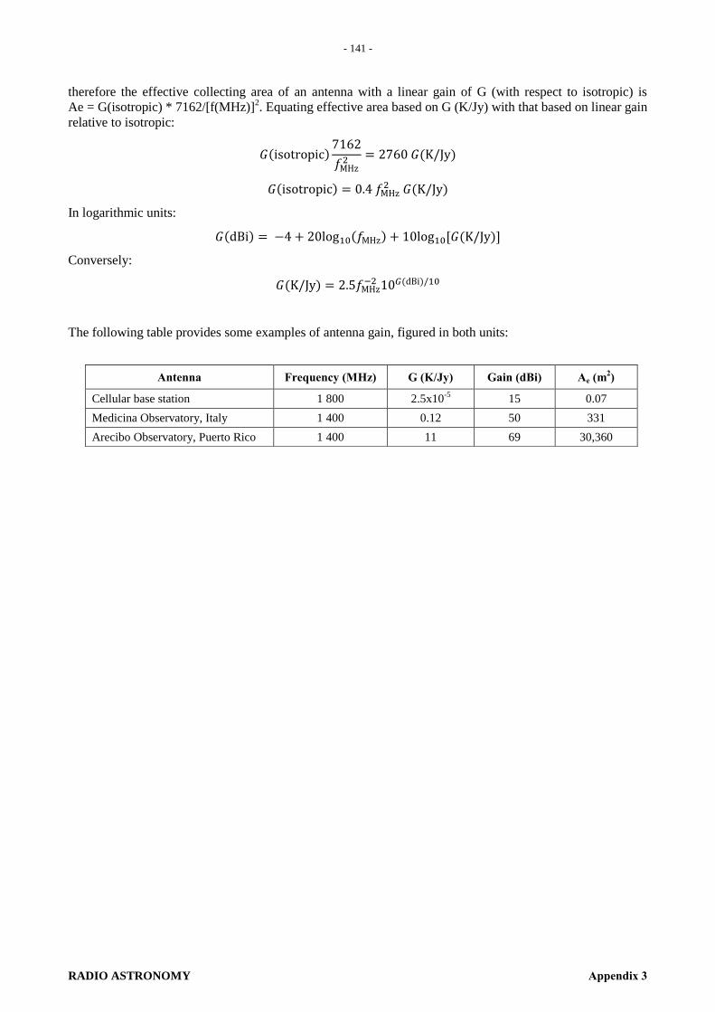
- 141 -
RADIO ASTRONOMY Appendix 3
– 1
41 –
therefore the effective collecting area of an antenna with a linear gain of G (with respect to isotropic) is
Ae = G(isotropic) * 7162/[f(MHz)]2. Equating effective area based on G (K/Jy) with that based on linear gain
relative to isotropic:
In logarithmic units:
Conversely:
The following table provides some examples of antenna gain, figured in both units:
Antenna Frequency (MHz) G (K/Jy) Gain (dBi) Ae (m2)
Cellular base station 1 800 2.5x10⁻⁵
15 0.07
Medicina Observatory, Italy 1 400 0.12 50 331
Arecibo Observatory, Puerto Rico 1 400 11 69 30,360
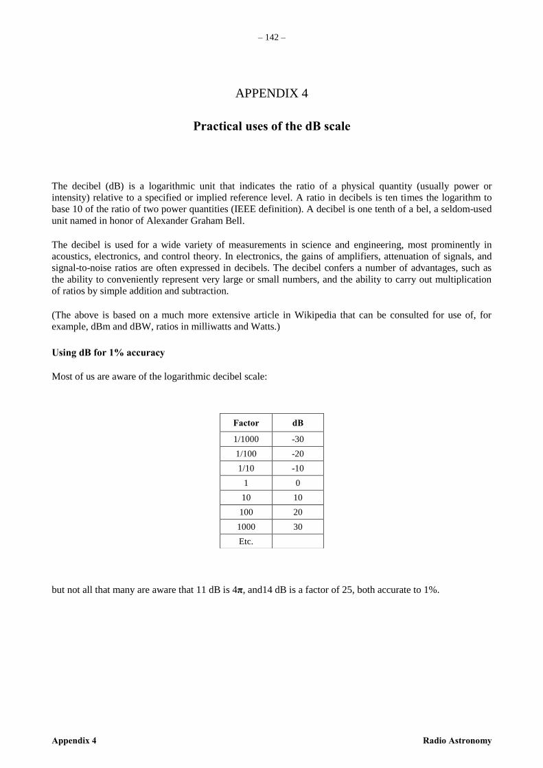
– 142 –
Appendix 4 Radio Astronomy
APPENDIX 4
Practical uses of the dB scale
The decibel (dB) is a logarithmic unit that indicates the ratio of a physical quantity (usually power or
intensity) relative to a specified or implied reference level. A ratio in decibels is ten times the logarithm to
base 10 of the ratio of two power quantities (IEEE definition). A decibel is one tenth of a bel, a seldom-used
unit named in honor of Alexander Graham Bell.
The decibel is used for a wide variety of measurements in science and engineering, most prominently in
acoustics, electronics, and control theory. In electronics, the gains of amplifiers, attenuation of signals, and
signal-to-noise ratios are often expressed in decibels. The decibel confers a number of advantages, such as
the ability to conveniently represent very large or small numbers, and the ability to carry out multiplication
of ratios by simple addition and subtraction.
(The above is based on a much more extensive article in Wikipedia that can be consulted for use of, for
example, dBm and dBW, ratios in milliwatts and Watts.)
Using dB for 1% accuracy
Most of us are aware of the logarithmic decibel scale:
but not all that many are aware that 11 dB is 4π, and14 dB is a factor of 25, both accurate to 1%.
Factor dB
1/1000 -30
1/100 -20
1/10 -10
1 0
10 10
100 20
1000 30
Etc.
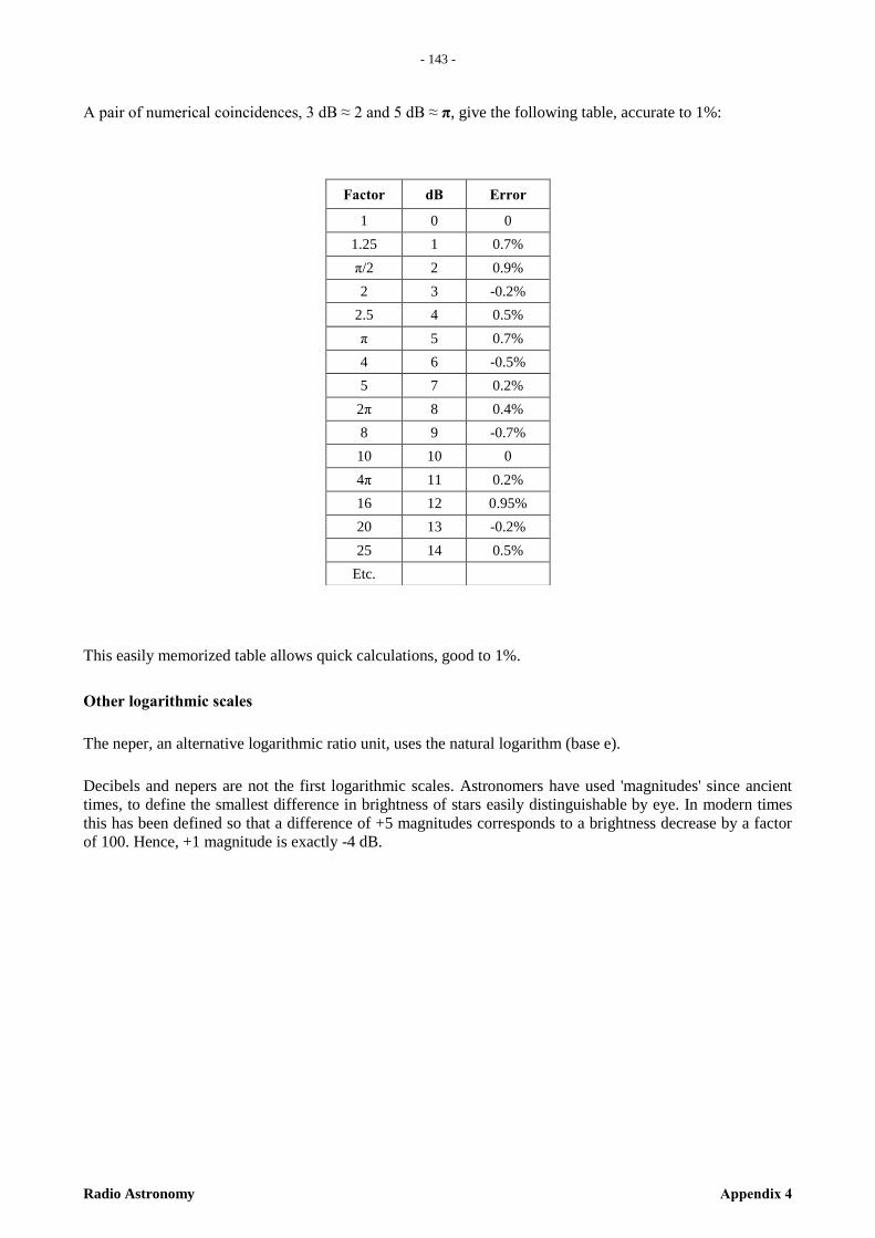
- 143 -
Radio Astronomy Appendix 4
– 1
43 –
A pair of numerical coincidences, 3 dB ≈ 2 and 5 dB ≈ π, give the following table, accurate to 1%:
This easily memorized table allows quick calculations, good to 1%.
Other logarithmic scales
The neper, an alternative logarithmic ratio unit, uses the natural logarithm (base e).
Decibels and nepers are not the first logarithmic scales. Astronomers have used 'magnitudes' since ancient
times, to define the smallest difference in brightness of stars easily distinguishable by eye. In modern times
this has been defined so that a difference of +5 magnitudes corresponds to a brightness decrease by a factor
of 100. Hence, +1 magnitude is exactly -4 dB.
Factor dB Error
1 0 0
1.25 1 0.7%
π/2 2 0.9%
2 3 -0.2%
2.5 4 0.5%
π 5 0.7%
4 6 -0.5%
5 7 0.2%
2π 8 0.4%
8 9 -0.7%
10 10 0
4π 11 0.2%
16 12 0.95%
20 13 -0.2%
25 14 0.5%
Etc.
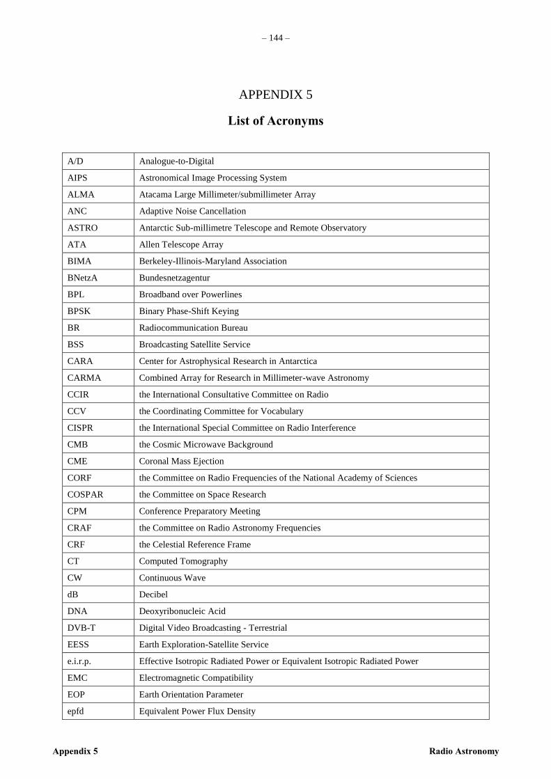
– 144 –
Appendix 5 Radio Astronomy
APPENDIX 5
List of Acronyms
A/D Analogue-to-Digital
AIPS Astronomical Image Processing System
ALMA Atacama Large Millimeter/submillimeter Array
ANC Adaptive Noise Cancellation
ASTRO Antarctic Sub-millimetre Telescope and Remote Observatory
ATA Allen Telescope Array
BIMA Berkeley-Illinois-Maryland Association
BNetzA Bundesnetzagentur
BPL Broadband over Powerlines
BPSK Binary Phase-Shift Keying
BR Radiocommunication Bureau
BSS Broadcasting Satellite Service
CARA Center for Astrophysical Research in Antarctica
CARMA Combined Array for Research in Millimeter-wave Astronomy
CCIR the International Consultative Committee on Radio
CCV the Coordinating Committee for Vocabulary
CISPR the International Special Committee on Radio Interference
CMB the Cosmic Microwave Background
CME Coronal Mass Ejection
CORF the Committee on Radio Frequencies of the National Academy of Sciences
COSPAR the Committee on Space Research
CPM Conference Preparatory Meeting
CRAF the Committee on Radio Astronomy Frequencies
CRF the Celestial Reference Frame
CT Computed Tomography
CW Continuous Wave
dB Decibel
DNA Deoxyribonucleic Acid
DVB-T Digital Video Broadcasting - Terrestrial
EESS Earth Exploration-Satellite Service
e.i.r.p. Effective Isotropic Radiated Power or Equivalent Isotropic Radiated Power
EMC Electromagnetic Compatibility
EOP Earth Orientation Parameter
epfd Equivalent Power Flux Density

- 145 -
Radio Astronomy Appendix 5
– 1
45 –
ESA European Space Agency
EU European Union
FET Field Effect Transistor
FFT Fast Fourier Transform
FPA Focal plane array
FSS Fixed Satellite Service
FX Fourier Transform before multiplication
GaAs FET Gallium Arsenide Field Effect Transistors
GBT Green Bank Telescope
GHz GigaHertz (= 1 000 000 000 Hertz)
GMRT Giant Metrewave Radio Telescope
GMSK Gaussian-filtered Minimum Shift Keying
GNSS Global Navigation Satellite System
GPS Global Positioning System
GSM Global System for Mobile Communications
GSO Geo-Stationary Orbit
HI Neutral Hydrogen
HII Ionised Hydrogen
HEMT High Electron Mobility Transistor
HF High Frequency
IAU the International Astronomical Union
ICSU the International Council of Scientific Unions
IEEE the Institute of Electrical and Electronics Engineers, Inc.
IF Intermediate Frequency
INR Interference to Noise Ratio
ISAS the Institute of Space and Astronautical Science
ISM Industrial, Scientific and Medical
ITU International Telecommunication Union
ITU-R the Radiocommunication Sector of the ITU
ITU-T the Telecommunication Standardization Sector of the ITU
IUCAF the Inter-Union Commission for the Allocation of Frequencies for Radio Astronomy and
Space Science
IVS International VLBI Service for Geodesy and Astronomy
JAXA Japan Aerospace Exploration Agency
JPL Jet Propulsion Laboratory
Jy Jansky (= 1 x 10-26
W/m2/Hz = -260 dB(W/m
2/Hz))
kHz KiloHertz (= 1 000 Hertz)
LAN Local Area Network
LEO Low Earth Orbit
LOFAR Low Frequency Array

– 146 –
Appendix 5 Radio Astronomy
LoS Line of Sight
LTE Long Term Evolution
MHz MigaHertz (= 1 000 000 Hertz)
MPIfR Max Planck Institut für Radioastronomie
MSS Mobile Satellite Service
MWA Murchison Widefield Array
NASA National Aeronautics and Space Administration
NDACC Network for Detection of Atmospheric Composition Change
NEA Near Earth Asteroid
NEO Near Earth Object
NIR Near Infrared
NRAO National Radio Astronomy Observatory
NRC National Research Council
NSF National Science Foundation (USA)
OoB Out-of-Band
OVRO Owens Valley Radio Observatory
pc parsec(=3.09x10¹⁶
m = 3.26 light year)
PET Positron Emission Tomography
pdf Power Flux Density
PLC Power Line Communications
PLT Power Line Telecommunications
PSK Phase-Shift Keying
RA Radiocommunication Assembly
RAFCAP the Radio Astronomy Frequency Committee in the Asia-Pacific Region
RAG the Radiocommunication Advisory Group
RAS Radio Astronomy Service
RF Radio Frequency
RFI Radio Frequency Interference
RLS Radiolocation service
rms Root Mean Square
RNSS Radionavigation Satellite Service
RQZ Radio Quiet Zone
RR Radio Regulations
RRB the Radio Regulations Board
SCRPM the Special Committee for Regulatory and Procedural Matters
SETI the Search for ExtraTerrestrial Intelligence
SFCG Space Frequency Coordination Group
SG Study Group
SIS Superconductor Insulator Superconductor
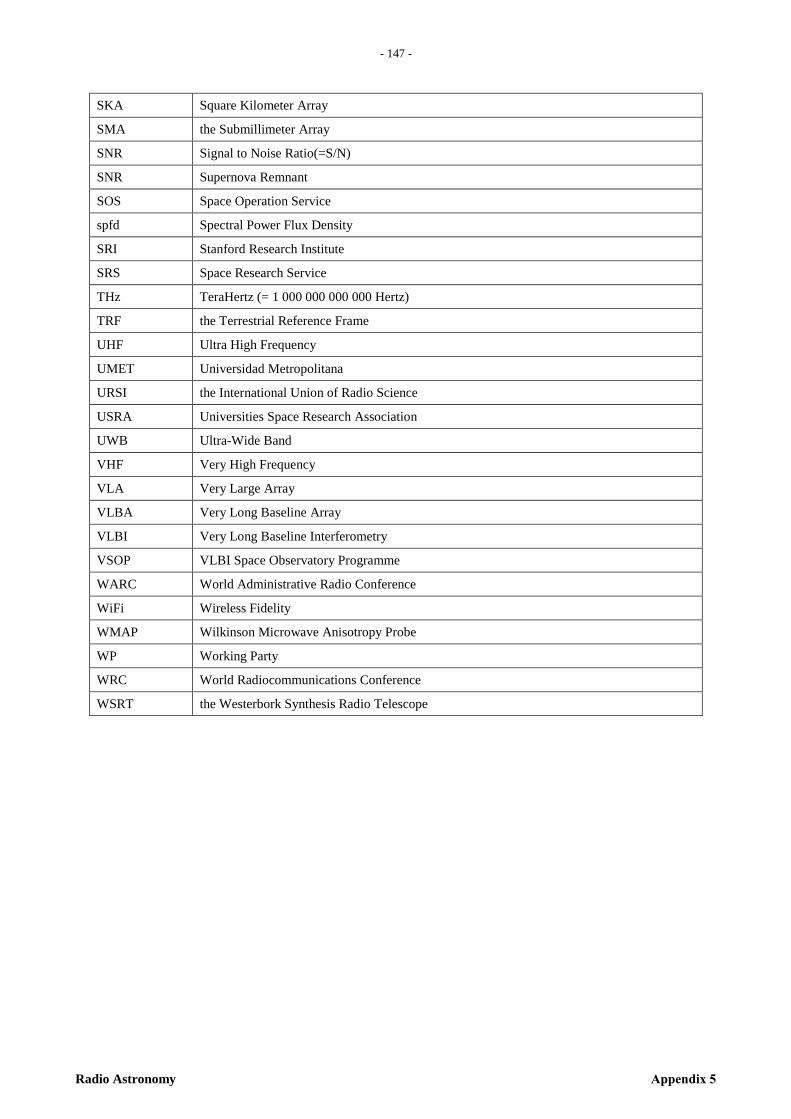
- 147 -
Radio Astronomy Appendix 5
– 1
47 –
SKA Square Kilometer Array
SMA the Submillimeter Array
SNR Signal to Noise Ratio(=S/N)
SNR Supernova Remnant
SOS Space Operation Service
spfd Spectral Power Flux Density
SRI Stanford Research Institute
SRS Space Research Service
THz TeraHertz (= 1 000 000 000 000 Hertz)
TRF the Terrestrial Reference Frame
UHF Ultra High Frequency
UMET Universidad Metropolitana
URSI the International Union of Radio Science
USRA Universities Space Research Association
UWB Ultra-Wide Band
VHF Very High Frequency
VLA Very Large Array
VLBA Very Long Baseline Array
VLBI Very Long Baseline Interferometry
VSOP VLBI Space Observatory Programme
WARC World Administrative Radio Conference
WiFi Wireless Fidelity
WMAP Wilkinson Microwave Anisotropy Probe
WP Working Party
WRC World Radiocommunications Conference
WSRT the Westerbork Synthesis Radio Telescope


HANDBOOK ON RADIO ASTRONOMY
Printed in Switzerland Geneva, 2013
ISBN: 978-92-61-14481-4 Photo credit: ATCA David Smyth
International Telecommunication Union
Sales and Marketing Division Place des Nations CH-1211 Geneva 20 Switzerland Fax: +41 22 730 5194 Tel.: +41 22 730 6141 E-mail: [email protected] Web: www.itu.int/publications
E d i t i o n o f 2 0 1 3Radiocommunication Bureau
*38650*
HANDBOOK ON RADIO ASTRONOMY
Edition of 2013