handling occlusions in dense multi-view stereo · handling occlusions in dense multi-view stereo...

Handling Occlusions in Dense Multi-view Stereo

Sing Bing Kang, Richard Szeliski, and Jinxiang Chai1

September 2001

Technical Report

MSR-TR-2001-80

While stereo matching was originally formulated as the recovery of 3D shape from

a pair of images, it is now generally recognized that using more than two images

can dramatically improve the quality of the reconstruction. Unfortunately, as more

images are added, the prevalence of semi-occluded regions (pixels visible in some but

not all images) also increases. In this paper, we propose some novel techniques to

deal with this problem. Our first idea is to use a combination of shiftable windows

and a dynamically selected subset of the neighboring images to do the matches. Our

second idea is to explicitly label occluded pixels within a global energy minimization

framework, and to reason about visibility within this framework so that only truly visible

pixels are matched. Experimental results show a dramatic improvement using the first

idea over conventional multibaseline stereo, especially when used in conjunction with

a global energy minimization technique. These results also show that explicit occlusion

labeling and visibility reasoning do help, but not significantly, if the spatial and temporal

selection is applied first.

Microsoft Research

Microsoft Corporation

One Microsoft Way

Redmond, WA 98052

http://www.research.microsoft.com

Longer version of a paper to be presented at the IEEE Computer Society Conference on

Computer Vision and Pattern Recognition (CVPR’2001), Kauai, Hawaii, December 2001.

1Current affiliation: The Robotics Institute, Carnegie Mellon University, Pittsburgh, PA 15213.

1 Introduction

One of the classic research problems in computer vision is that of stereo, i.e., the reconstruction

of three-dimensional shape from two or more intensity images. Such reconstruction has many

practical applications, including robot navigation, object recognition, and more recently, realistic

scene visualization (image-based rendering).

Why is stereo so difficult? Even if we disregard non-rigid effects such as specularities, reflec-

tions, and transparencies, a complete and general solution to stereo has yet to be found. This can be

attributed to depth discontinuities, which cause occlusions and disocclusions, and to lack of texture

in images. Depth discontinuities cause objects to appear and disappear at different viewpoints, thus

confounding the matching process at or near object boundaries. The lack of texture, meanwhile,

results in ambiguities in depth assignments caused by the presence of multiple good matches.

1.1 Previous work

A substantial amount of work has been done on stereo; a survey on stereo methods can be found

in [DA89]. Stereo can generally be described in terms of the following components: matching

criterion, aggregation method, and winner selection [SS98, SZ99].

1.1.1 Matching criterion

The matching criterion is used as a means of measuring the similarity of pixels or regions across

different images. A typical error measure is the RGB or intensity difference between images (these

differences can be squared, or robust measures can be used). Some methods compute subpixel

disparities by computing the analytic minimum of the local error surface [MSK89] or using gradient-

based techniques [LK81, ST94, SC97]. Birchfield and Tomasi [BT98] measure pixel dissimilarity

by taking the minimum difference between a pixel in one image and the interpolated intensity

function in the other image.

1.1.2 Aggregation method

The aggregation method refers to the manner in which the error function over the search space

is computed or accumulated. The most direct way is to apply search windows of a fixed size

over a prescribed disparity space for multiple cameras [OK93] or for verged camera configuration

1

[KWZK95]. Others use adaptive windows [OK92], shiftable windows [Arn83, BI99, TSK01],

or multiple masks [NMSO96]. Another set of methods accumulates votes in 3D space, e.g., the

space sweep approach [Col96] and voxel coloring and its variants [SD97, SG99, KS99]. More

sophisticated methods take into account occlusion in the formulation, for example, by erasing pixels

once they have been matched [SD97, SG99, KS99], by estimating a depth map per image [Sze99],

or using prior color-based segmentation followed by iterative analysis-by-synthesis [TSK01].

1.1.3 Optimization and winner selection

Once the initial or aggregated matching costs have been computed, a decision must be made as

to the correct disparity assignment for each pixel d(x, y). Local methods do this at each pixel

independently, typically by picking the disparity with the minimum aggregated value. Multires-

olution approaches have also been used [BAHH92, Han91, SC94] to guide the winner selection

search. Cooperative/competitive algorithms can be used to iteratively decide on the best assignments

[MP79, SS98, ZK00].

Dynamic programming can be used for computing depths associated with edge features [OK85]

or general intensity similarity matches. These approaches can take advantage of one-dimensional

ordering constraints along the epipolar line to handle depth discontinuities and unmatched regions

[GLY92, Bel96, BI99]. However, these techniques are limited to two frames.

Fully global methods attempt to find a disparity surface d(x, y) that minimizes some smooth-

ness or regularity property in addition to producing good matches. Such approaches include surface

model fitting [HA86], regularization [PTK85, Ter86, SC97] Markov Random Field optimization

with simulated annealing [GG84, MMP87, Bar89], nonlinear diffusion of support at different dis-

parity hypotheses [SS98], graph cut methods [RC98, IG98, BVZ99], and the use of graph cuts in

conjuction with planar surface fitting [BT99].

1.1.4 Using layers and regions

Many techniques have resorted to using layers to handle scenes with possible textureless regions

and large amounts of occlusion. One of the first techniques, in the context of image compression,

uses affine models [WA93]. This was later further developed in various ways: smoothness within

layers [Wei97], “skin and bones” [JBJ96] and additive models [SAA00] to handle transparency,

and depth reconstruction from multiple images [BSA98].

2

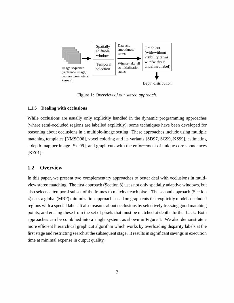
Image sequence(reference image,camera parametersknown)

Spatiallyshiftablewindows

Temporalselection

Winner-take-allas initializationstates

Data andsmoothnessterms

Graph cut(with/withoutvisibility terms,with/withoutundefined label)

Depth distribution

Figure 1: Overview of our stereo approach.

1.1.5 Dealing with occlusions

While occlusions are usually only explicitly handled in the dynamic programming approaches

(where semi-occluded regions are labelled explicitly), some techniques have been developed for

reasoning about occlusions in a multiple-image setting. These approaches include using multiple

matching templates [NMSO96], voxel coloring and its variants [SD97, SG99, KS99], estimating

a depth map per image [Sze99], and graph cuts with the enforcement of unique correspondences

[KZ01].

1.2 Overview

In this paper, we present two complementary approaches to better deal with occlusions in multi-

view stereo matching. The first approach (Section 3) uses not only spatially adaptive windows, but

also selects a temporal subset of the frames to match at each pixel. The second approach (Section

4) uses a global (MRF) minimization approach based on graph cuts that explicitly models occluded

regions with a special label. It also reasons about occlusions by selectively freezing good matching

points, and erasing these from the set of pixels that must be matched at depths further back. Both

approaches can be combined into a single system, as shown in Figure 1. We also demonstrate a

more efficient hierarchical graph cut algorithm which works by overloading disparity labels at the

first stage and restricting search at the subsequent stage. It results in significant savings in execution

time at minimal expense in output quality.

3

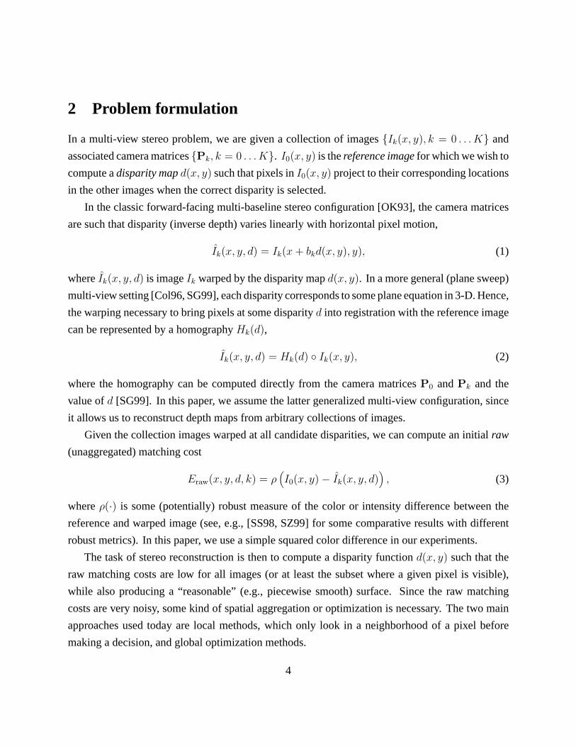
2 Problem formulation

In a multi-view stereo problem, we are given a collection of images {Ik(x, y), k = 0 . . . K} and

associated camera matrices {Pk, k = 0 . . . K}. I0(x, y) is the reference image for which we wish to

compute a disparity map d(x, y) such that pixels in I0(x, y) project to their corresponding locations

in the other images when the correct disparity is selected.

In the classic forward-facing multi-baseline stereo configuration [OK93], the camera matrices

are such that disparity (inverse depth) varies linearly with horizontal pixel motion,

Ik(x, y, d) = Ik(x + bkd(x, y), y), (1)

where Ik(x, y, d) is image Ik warped by the disparity map d(x, y). In a more general (plane sweep)

multi-view setting [Col96, SG99], each disparity corresponds to some plane equation in 3-D. Hence,

the warping necessary to bring pixels at some disparity d into registration with the reference image

can be represented by a homography Hk(d),

Ik(x, y, d) = Hk(d) ◦ Ik(x, y), (2)

where the homography can be computed directly from the camera matrices P0 and Pk and the

value of d [SG99]. In this paper, we assume the latter generalized multi-view configuration, since

it allows us to reconstruct depth maps from arbitrary collections of images.

Given the collection images warped at all candidate disparities, we can compute an initial raw

(unaggregated) matching cost

Eraw(x, y, d, k) = ρ(I0(x, y) − Ik(x, y, d)

), (3)

where ρ(·) is some (potentially) robust measure of the color or intensity difference between the

reference and warped image (see, e.g., [SS98, SZ99] for some comparative results with different

robust metrics). In this paper, we use a simple squared color difference in our experiments.

The task of stereo reconstruction is then to compute a disparity function d(x, y) such that the

raw matching costs are low for all images (or at least the subset where a given pixel is visible),

while also producing a “reasonable” (e.g., piecewise smooth) surface. Since the raw matching

costs are very noisy, some kind of spatial aggregation or optimization is necessary. The two main

approaches used today are local methods, which only look in a neighborhood of a pixel before

making a decision, and global optimization methods.

4

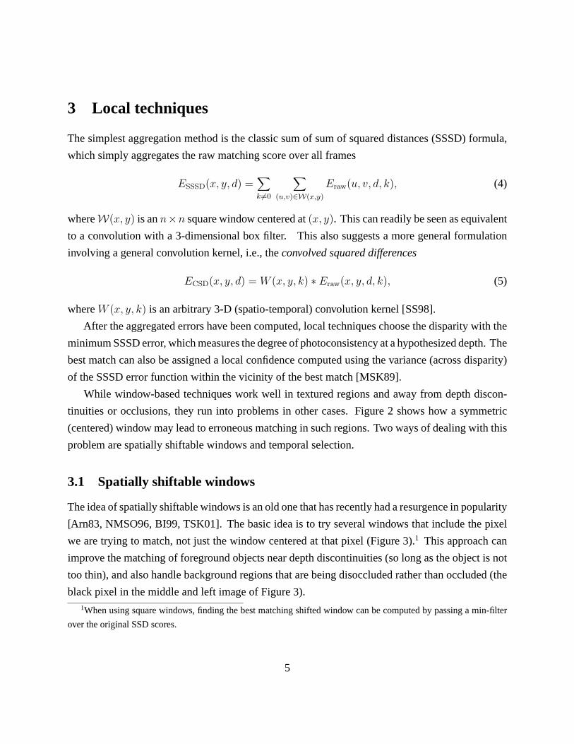
3 Local techniques

The simplest aggregation method is the classic sum of sum of squared distances (SSSD) formula,

which simply aggregates the raw matching score over all frames

ESSSD(x, y, d) =∑k �=0

∑(u,v)∈W(x,y)

Eraw(u, v, d, k), (4)

where W(x, y) is an n×n square window centered at (x, y). This can readily be seen as equivalent

to a convolution with a 3-dimensional box filter. This also suggests a more general formulation

involving a general convolution kernel, i.e., the convolved squared differences

ECSD(x, y, d) = W (x, y, k) ∗ Eraw(x, y, d, k), (5)

where W (x, y, k) is an arbitrary 3-D (spatio-temporal) convolution kernel [SS98].

After the aggregated errors have been computed, local techniques choose the disparity with the

minimum SSSD error, which measures the degree of photoconsistency at a hypothesized depth. The

best match can also be assigned a local confidence computed using the variance (across disparity)

of the SSSD error function within the vicinity of the best match [MSK89].

While window-based techniques work well in textured regions and away from depth discon-

tinuities or occlusions, they run into problems in other cases. Figure 2 shows how a symmetric

(centered) window may lead to erroneous matching in such regions. Two ways of dealing with this

problem are spatially shiftable windows and temporal selection.

3.1 Spatially shiftable windows

The idea of spatially shiftable windows is an old one that has recently had a resurgence in popularity

[Arn83, NMSO96, BI99, TSK01]. The basic idea is to try several windows that include the pixel

we are trying to match, not just the window centered at that pixel (Figure 3).1 This approach can

improve the matching of foreground objects near depth discontinuities (so long as the object is not

too thin), and also handle background regions that are being disoccluded rather than occluded (the

black pixel in the middle and left image of Figure 3).1When using square windows, finding the best matching shifted window can be computed by passing a min-filter

over the original SSD scores.

5

A

B C D EF

A

B C D EF

A

B C D EF

left middle right

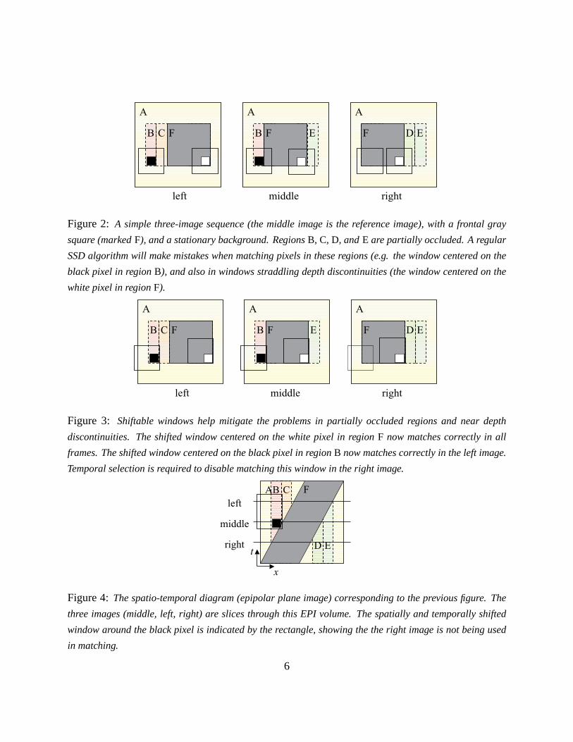
Figure 2: A simple three-image sequence (the middle image is the reference image), with a frontal gray

square (marked F), and a stationary background. Regions B, C, D, and E are partially occluded. A regular

SSD algorithm will make mistakes when matching pixels in these regions (e.g. the window centered on the

black pixel in region B), and also in windows straddling depth discontinuities (the window centered on the

white pixel in region F).

A

B C D EF

A

B C D EF

A

B C D EF

left middle right

Figure 3: Shiftable windows help mitigate the problems in partially occluded regions and near depth

discontinuities. The shifted window centered on the white pixel in region F now matches correctly in all

frames. The shifted window centered on the black pixel in region B now matches correctly in the left image.

Temporal selection is required to disable matching this window in the right image.

A

ED

CBleft

middle

right

F

x

t

Figure 4: The spatio-temporal diagram (epipolar plane image) corresponding to the previous figure. The

three images (middle, left, right) are slices through this EPI volume. The spatially and temporally shifted

window around the black pixel is indicated by the rectangle, showing the the right image is not being used

in matching.

6

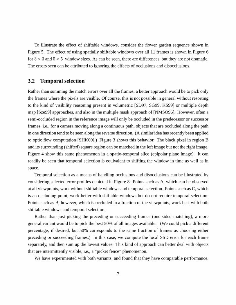
To illustrate the effect of shiftable windows, consider the flower garden sequence shown in

Figure 5. The effect of using spatially shiftable windows over all 11 frames is shown in Figure 6

for 3 × 3 and 5 × 5 window sizes. As can be seen, there are differences, but they are not dramatic.

The errors seen can be attributed to ignoring the effects of occlusions and disocclusions.

3.2 Temporal selection

Rather than summing the match errors over all the frames, a better approach would be to pick only

the frames where the pixels are visible. Of course, this is not possible in general without resorting

to the kind of visibility reasoning present in volumetric [SD97, SG99, KS99] or multiple depth

map [Sze99] approaches, and also in the multiple mask approach of [NMSO96]. However, often a

semi-occluded region in the reference image will only be occluded in the predecessor or successor

frames, i.e., for a camera moving along a continuous path, objects that are occluded along the path

in one direction tend to be seen along the reverse direction. (A similar idea has recently been applied

to optic flow computation [SHK00].) Figure 3 shows this behavior. The black pixel in region B

and its surrounding (shifted) square region can be matched in the left image but not the right image.

Figure 4 show this same phenomenon in a spatio-temporal slice (epipolar plane image). It can

readily be seen that temporal selection is equivalent to shifting the window in time as well as in

space.

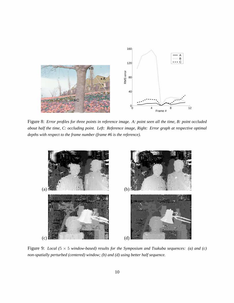
Temporal selection as a means of handling occlusions and disocclusions can be illustrated by

considering selected error profiles depicted in Figure 8. Points such as A, which can be observed

at all viewpoints, work without shiftable windows and temporal selection. Points such as C, which

is an occluding point, work better with shiftable windows but do not require temporal selection.

Points such as B, however, which is occluded in a fraction of the viewpoints, work best with both

shiftable windows and temporal selection.

Rather than just picking the preceding or succeeding frames (one-sided matching), a more

general variant would be to pick the best 50% of all images available. (We could pick a different

percentage, if desired, but 50% corresponds to the same fraction of frames as choosing either

preceding or succeeding frames.) In this case, we compute the local SSD error for each frame

separately, and then sum up the lowest values. This kind of approach can better deal with objects

that are intermittently visible, i.e., a “picket fence” phenomenon.

We have experimented with both variants, and found that they have comparable performance.

7

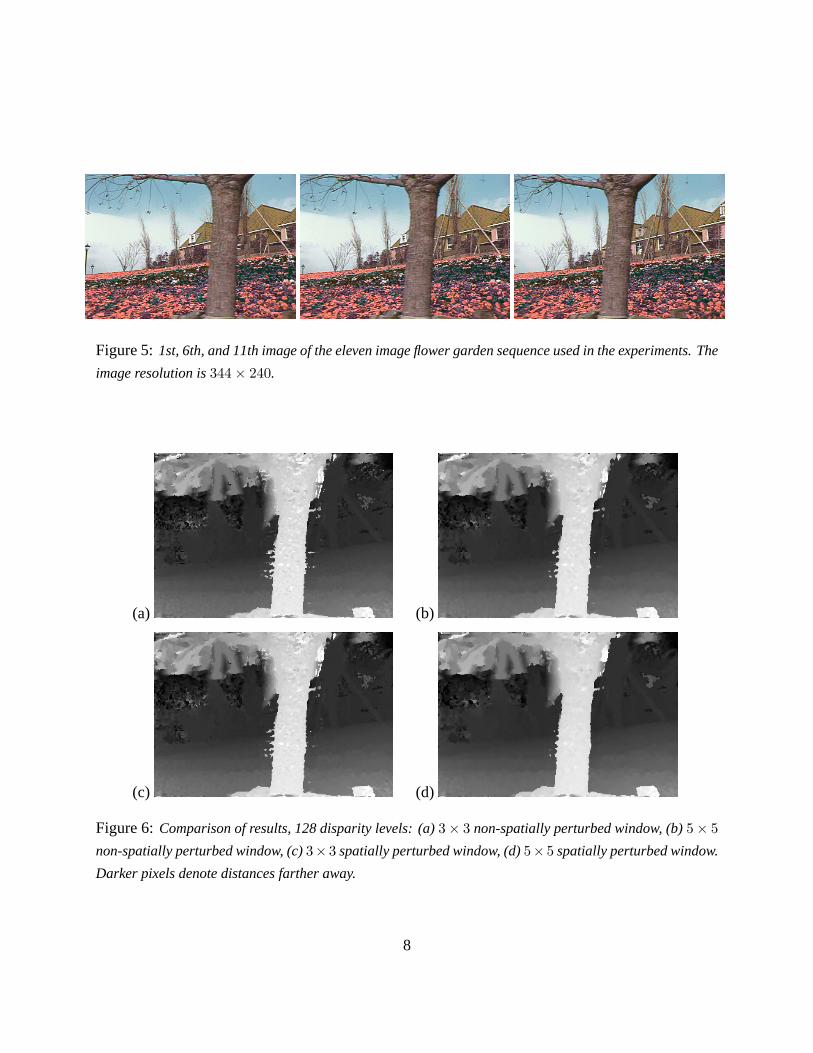
Figure 5: 1st, 6th, and 11th image of the eleven image flower garden sequence used in the experiments. The

image resolution is 344 × 240.

(a) (b)

(c) (d)

Figure 6: Comparison of results, 128 disparity levels: (a) 3 × 3 non-spatially perturbed window, (b) 5 × 5

non-spatially perturbed window, (c) 3× 3 spatially perturbed window, (d) 5× 5 spatially perturbed window.

Darker pixels denote distances farther away.

8

(a) (b)

(c) (d)

(e) (f)

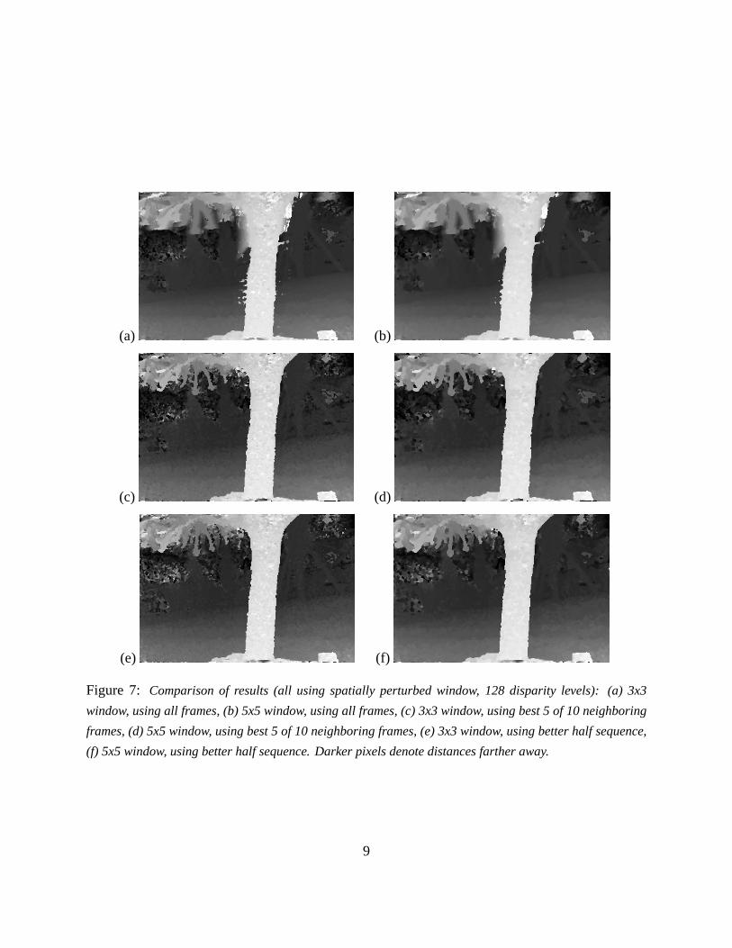
Figure 7: Comparison of results (all using spatially perturbed window, 128 disparity levels): (a) 3x3

window, using all frames, (b) 5x5 window, using all frames, (c) 3x3 window, using best 5 of 10 neighboring

frames, (d) 5x5 window, using best 5 of 10 neighboring frames, (e) 3x3 window, using better half sequence,

(f) 5x5 window, using better half sequence. Darker pixels denote distances farther away.

9

0 4 8 120

40

80

120

160

Frame #

RM

S e

rror

ABC

Figure 8: Error profiles for three points in reference image. A: point seen all the time, B: point occluded

about half the time, C: occluding point. Left: Reference image, Right: Error graph at respective optimal

depths with respect to the frame number (frame #6 is the reference).

(a) (b)

(c) (d)

Figure 9: Local (5 × 5 window-based) results for the Symposium and Tsukuba sequences: (a) and (c)

non-spatially perturbed (centered) window; (b) and (d) using better half sequence.

10

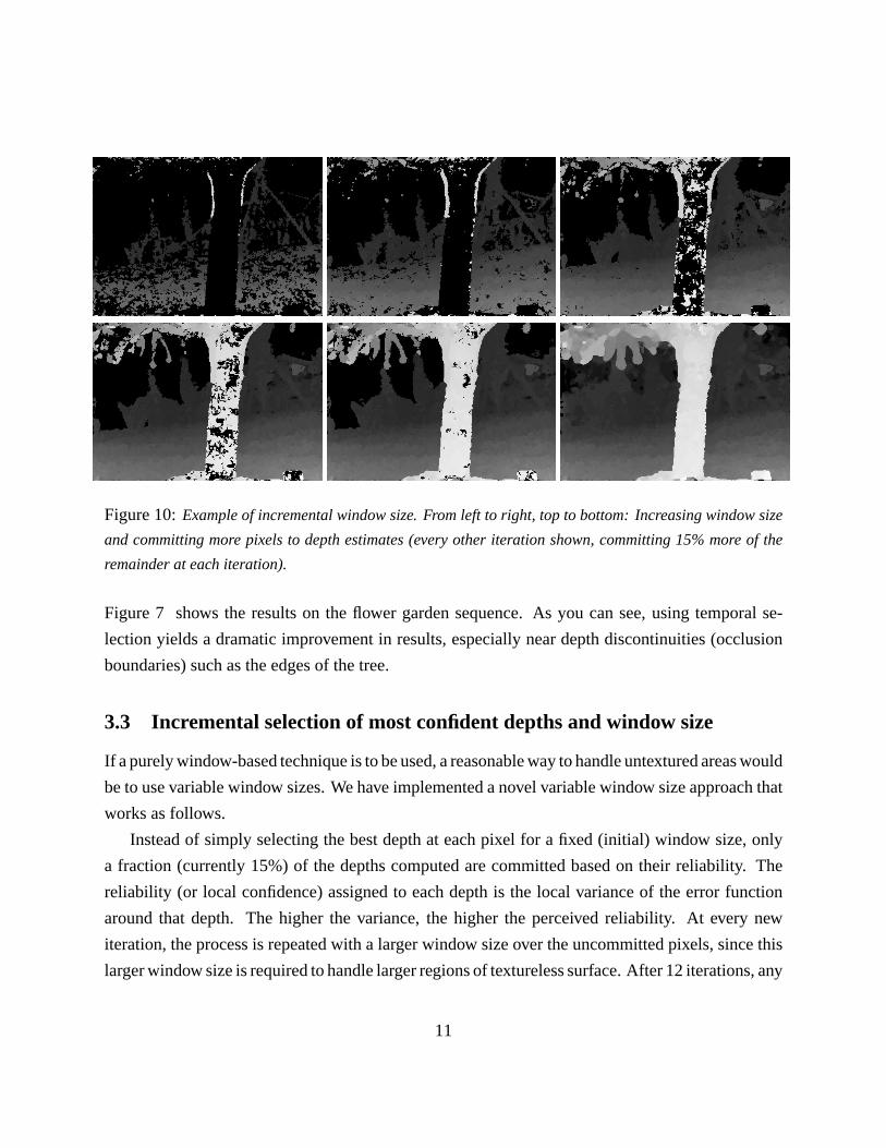
Figure 10: Example of incremental window size. From left to right, top to bottom: Increasing window size

and committing more pixels to depth estimates (every other iteration shown, committing 15% more of the

remainder at each iteration).

Figure 7 shows the results on the flower garden sequence. As you can see, using temporal se-

lection yields a dramatic improvement in results, especially near depth discontinuities (occlusion

boundaries) such as the edges of the tree.

3.3 Incremental selection of most confident depths and window size

If a purely window-based technique is to be used, a reasonable way to handle untextured areas would

be to use variable window sizes. We have implemented a novel variable window size approach that

works as follows.

Instead of simply selecting the best depth at each pixel for a fixed (initial) window size, only

a fraction (currently 15%) of the depths computed are committed based on their reliability. The

reliability (or local confidence) assigned to each depth is the local variance of the error function

around that depth. The higher the variance, the higher the perceived reliability. At every new

iteration, the process is repeated with a larger window size over the uncommitted pixels, since this

larger window size is required to handle larger regions of textureless surface. After 12 iterations, any

11

undecided pixels are forced to commit. By using the error variance as a measure of depth reliability,

we ensure that larger regions of textureless surfaces get to be handled by larger windows.

Our approach bears some resemblance to the recent proposal by Zhang and Shan [ZS00],

which starts with point matches and grows matching regions around these points. In our approach,

however, there is no requirement to grow existing regions; instead, the most confident pixels are

simply selected at each iteration. Our idea of variable window sizes is also similar to [OK92].

However, we adopt a highest confidence first approach [CB90] to choosing a window size rather

than testing at each pixel location all the windows sizes in order to select an optimal size.

Results of using the incremental selection approach can be seen in Figure 10, Figure 12 (for

sequence shown in Figure 11), and Figure 14 (for sequence shown in Figure 13). While it generally

interpolates across textureless regions reasonably well, determining the correct fraction of pixels

to commit at each iteration requires a heuristic decision (i.e., it may be scene dependent).

4 Global techniques

The second general approach to dealing with ambiguity in stereo correspondence is to optimize a

global energy function. Typically, such a function consists of two terms,

Eglobal(d(x, y)) = Edata + Esmooth. (6)

The value of the disparity field d(x, y) that minimizes this global energy is chosen as the desired

solution.2

The data term Edata is just a summation of the local (aggregated or unaggregated) matching

costs, e.g.,

Edata =∑(x,y)

ESSSD(x, y, d(x, y)). (7)

Because a smoothness term is used, spatial aggregation is usually not used, i.e., the window W (x, y)in the SSSD term is a single pixel (but see, e.g., [BI99] for a global method that starts with a window-

based cost measure).2Because of the tight connection between this kind of global energy and the log-likelihood of a Bayesian model

using Markov Random Fields, these methods are also often called Bayesian or MRF methods [GG84, Bel96, BVZ99].

12

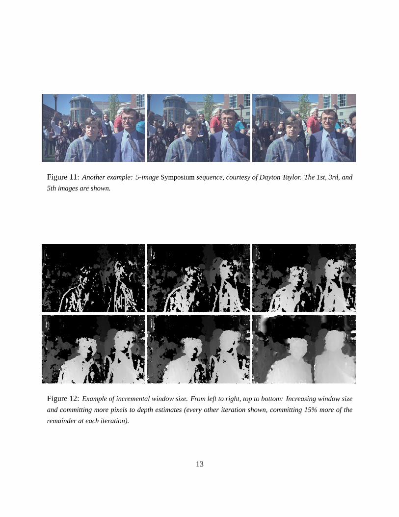
Figure 11: Another example: 5-image Symposium sequence, courtesy of Dayton Taylor. The 1st, 3rd, and

5th images are shown.




13

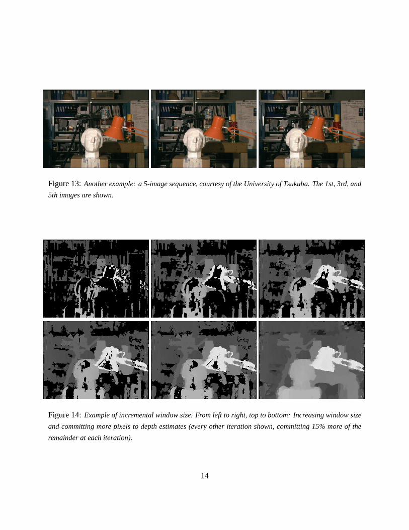
Figure 13: Another example: a 5-image sequence, courtesy of the University of Tsukuba. The 1st, 3rd, and

5th images are shown.




14

The smoothness term Esmooth measures the piecewise-smoothness in the disparity field,

Esmooth =∑(x,y)

shx,yφ(d(x, y) − d(x + 1, y)) (8)

+ svx,yφ(d(x, y) − d(x, y + 1)).

The smoothness potential φ(·) can be a simple quadratic, a delta function, a truncated quadratic, or

some other robust function of the disparity differences [BR96, BVZ99]. The smoothness strengths

shx,y and sv

x,y can be spatially varying (or even tied to additional variables called line processes

[GG84, BR96]). The MRF formulation used by [BVZ99] makes shx,y and sv

x,y monotonic functions of

the local intensity gradient, which greatly helps in forcing disparity discontinuities to be coincident

with intensity discontinuities.

If the vertical smoothness term is ignored, the global minimization can be decomposed into an

independent set of 1-D optimizations, for which efficient dynamic programming algorithms exist

[GLY92, Bel96, BI99]. Many different algorithms have also been developed for minimizing the

full 2-D global energy function, e.g., [GG84, PTK85, Ter86, SC97, SS98, RC98, IG98, BVZ99].

In this section, we propose a number of extensions to the graph cut formulation introduced by

[BVZ99] in order to better handle the partial occlusions that occur in multi-view stereo: explicit

occluded pixel labeling, visibility computation, and hierarchical disparity computation.

4.1 Explicit occluded pixel labeling

When using a global optimization framework, pixels that do not have good matches in other images

will still be assigned some disparity. Such pixels are often associated with a high local matching

cost, and can be detected in a post-processing phase. However, occluded pixels also tend to occur

in contiguous regions, so it makes sense to include this information within the smoothness function

(i.e., within the MRF formulation).

Our solution to this problem is to include an additional label that indicates pixels that are either

outliers or potentially occluded. A fixed penalty is associated with adopting this label, as opposed to

the local matching cost associated with some other disparity label. (In our current implementation,

this penalty is set at 18 intensity levels.) The penalty should be set to be somewhat higher that the

largest value observed for correctly matching pixels. The smoothness term for this label is a delta

function, i.e., a fixed penalty is paid for every non-occluded pixel that borders an occluded one.

15

Figure 15: Effect of using the undefined label for 11-frame flower garden sequence (64 depth levels, no

visibility terms, using best frames): (a) Reference image is 1st image, (b) Reference image is 6th image, (c)

Reference image is 11th image. The undefined label is red, while the intensities for the rest are bumped up

for visual clarity.

Examples of using such a label can be seen in Figure 15. Unfortunately, this approach sometimes

fails to correctly label pixels in occluded textureless regions (since these pixels may still match

correctly at the frontal depth). In addition, the optimal occluded label penalty setting depends on

the amount of contrast in a given scene.

4.2 Visibility reasoning

An idea that has proven to be very effective in dealing with occlusions in volumetric [SD97, SG99,

KS99] or multiple depth map [Sze99] approaches is that of visibility reasoning. Once a pixel has

been matched at one disparity level, it is possible to “erase” that pixel from consideration when

considering possible matches at disparities further back. This is the most principled way to reason

about visibility and partial occlusions in multi-view stereo. However, since the algorithms cited

above make independent decisions between pixels or frames, their results may not be optimal.

To incorporate visibility into the global optimization framework, we compute a visibility func-

tion similar to the one presented in [SG99]. The visibility function v(x, y, d, k) can be computed as

a function of the disparity assignments at layers closer than d. Let o(x, y, d′) = δ(d′, d(x, y)) be the

opacity (or indicator) function, i.e., a binary image of those pixels assigned to level d′. The shadow

s(x, y, d′, d, k) that this opacity casts relative to camera k onto another level d can be derived from

the homographies that map between disparities d′ and d

s(x, y, d′, d, k) = (Hk(d)H−1k (d′)) ◦ o(x, y, d′) (9)

16

(we can, for instance, use bilinear resampling to get “soft” shadows, indicative of partial visibility).

The visibility of a pixel (x, y) at disparity d relative to camera k can be computed as

v(x, y, d, k) =∏d′<d

(1 − s(x, y, d′, d, k)). (10)

Finally, the raw matching cost (3) can then be replaced by

Evis(x, y, d, k) = v(x, y, d, k)ρ(I0(x, y) − Ik(x, y, d)

). (11)

The above visibility-modulated matching score thus provides a principled way to compute the

goodness of a particular disparity map d(x, y) while explicitly taking into account occlusions and

partial visibility. For any given labeling d(x, y), we can compute the opacities, shadows, and

visibilities, and then sum up the visibility-modulated matching scores (11) to obtain the final global

energy (6). Unfortunately, it is not obvious how to minimize such a complicated energy function.

One possibility would be to start with all pixels visible, and to then run the usual graph-cut

algorithm. From the initial d(x, y) solution, we could recompute visibilities, and then re-optimize

the modified energy function. Unfortunately, this process may not converge, since the energy

function is being modified from iteration to iteration, and the visibilities assumed for one iteration

may be undone by a re-assignment of labels in that iteration.

The alternative we have come up with (inspired by Chou’s Highest Confidence First algorithm

[CB90]) is to progressively commit the best-matching depths (i.e., freeze their labels) and apply

graph cut on the remaining pixels. This approach is related to the voxel coloring work [SD97], where

voxels are tagged from front to back. However, in our approach, the best 15% of the pixels (based

on the current visibility-modulated matching score (11)) whose depths have been computed by the

graph cut are frozen. The visibility function and matching costs are then recomputed, which may

affect costs at more distal voxels. Within each iteration, graph-cut labeling effectively takes into

account neighboring pixels’ preferences and tries to make the disparity function piecewise-smooth,

whereas the voxel coloring approach only uses per-pixel photo-consistency. After 12 iterations, the

remaining uncommitted pixels are frozen at their best value.

Thus, our multiview stereo algorithm uses a combination of HCF and graph-cut optimization

of a global energy with visibility terms. Its steps are:

1. Run a plane sweep to compute the local matcing costs, which are then used for initializing

the data terms for a graph cut algorithm. The color reference image is used to set the spatial

smoothness terms.

17

2. Iterate the following:

(a) Run the graph cut minimization algorithm

(b) Compute confidence associated with the depths that has not been frozen, and freeze a

portion of them (15% in our case)

(c) Recompute the data terms with visibility taken into account as a result of the frozen

depths.

Step 2 is repeated for a maximum number of times (12 in our case). At the last iteration, all

remaining pixels are committed. Depths are frozen by setting data costs associated with other depths

very high (108 in our case). The visibility terms v(x, y, d, k) in (10) are computed by performing a

front-to-back sweep and masking out pixels from non-reference views as they are touched by the

frozen depths in the reference view, as described above.

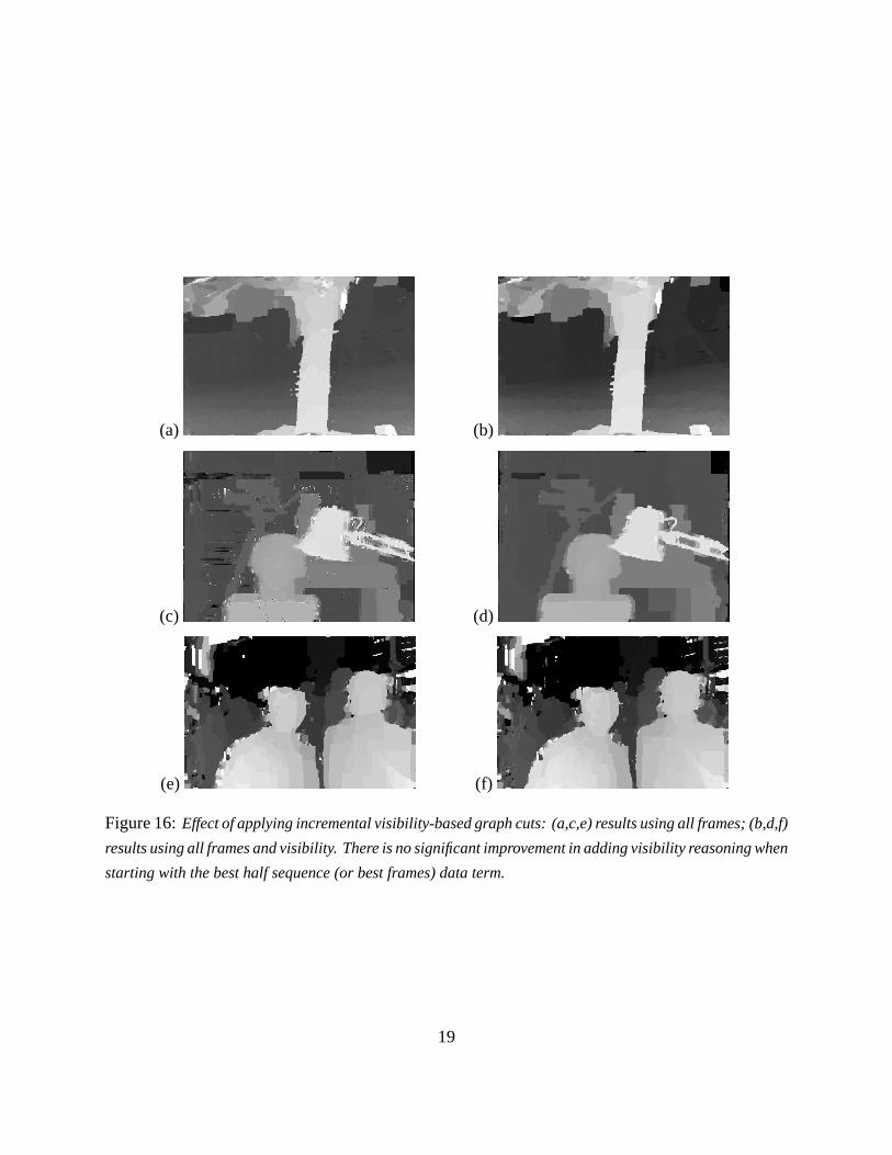
Figure 16 shows the results of adding visibility reasoning to the graph cut algorithm when starting

with all frames as the data cost (no temporal selection). As can be seen by comparing the first two

columns, the improvement is significant. Surprisingly, the addition of visibility computation to the

graph cut did not produce significant improvements to our algorithm when the original matching

costs were computed using a shiftable window and temporal selection. This suggests that the

shiftable window, and especially temporal selection, handled the occlusion problem well.

4.3 Hierarchical disparity computation

While the graph cut algorithm and its variants can produce very good results, the problem of

computing the exact minimum via graph cuts is NP-hard [Vek99]. Furthermore, the complexity of

the approximated algorithm is quadratic in the number of labels. As a result, we need to keep the

number of labels (in the form of disparities) to a minimum.

To reduce the severity of this problem, we first solve the graph cut algorithm using a smaller

number of labels, and then solve for an assignment at the desired final resolution level. In the

first phase, each overloaded label represents a range of disparity values, as indicated in Figure 17.

The cost function associated with a label is the minimum of the costs associated with its range of

disparity values, i.e.,

C∗(u, v, d′k) = min

di∈d′k

C(u, v, di). (12)

18

(a) (b)

(c) (d)

(e) (f)

Figure 16: Effect of applying incremental visibility-based graph cuts: (a,c,e) results using all frames; (b,d,f)

results using all frames and visibility. There is no significant improvement in adding visibility reasoning when

starting with the best half sequence (or best frames) data term.

19

d’k

d’0

d’N-1

d0...

dR-1

dRk

dR(k+1)-1

dR(N-1)

dRN-1

......

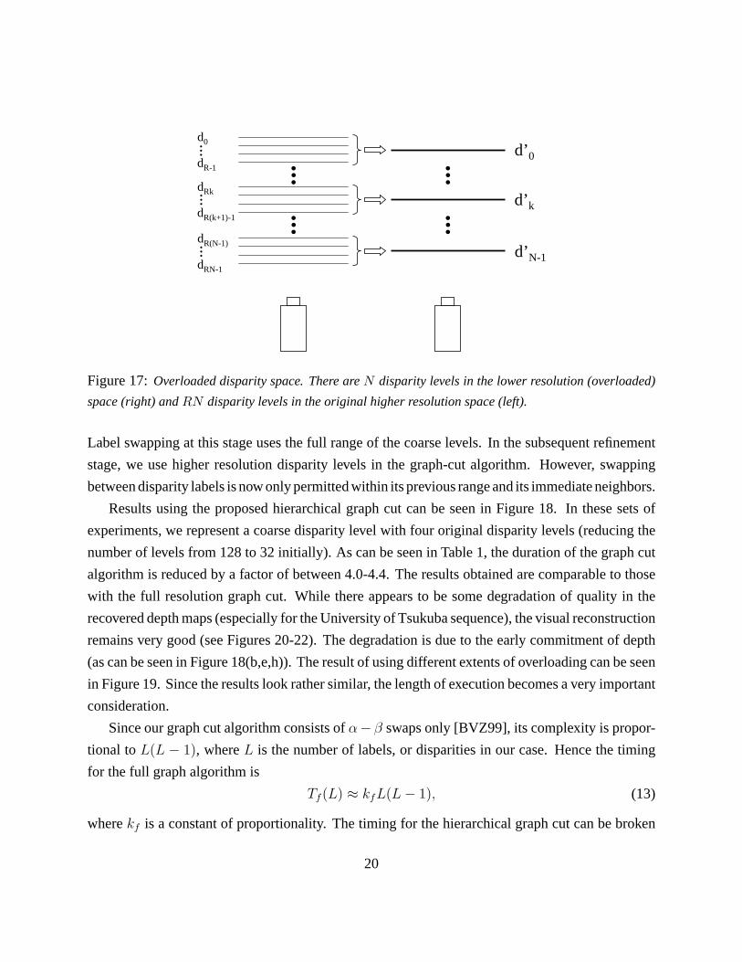
Figure 17: Overloaded disparity space. There are N disparity levels in the lower resolution (overloaded)

space (right) and RN disparity levels in the original higher resolution space (left).

Label swapping at this stage uses the full range of the coarse levels. In the subsequent refinement

stage, we use higher resolution disparity levels in the graph-cut algorithm. However, swapping

between disparity labels is now only permitted within its previous range and its immediate neighbors.

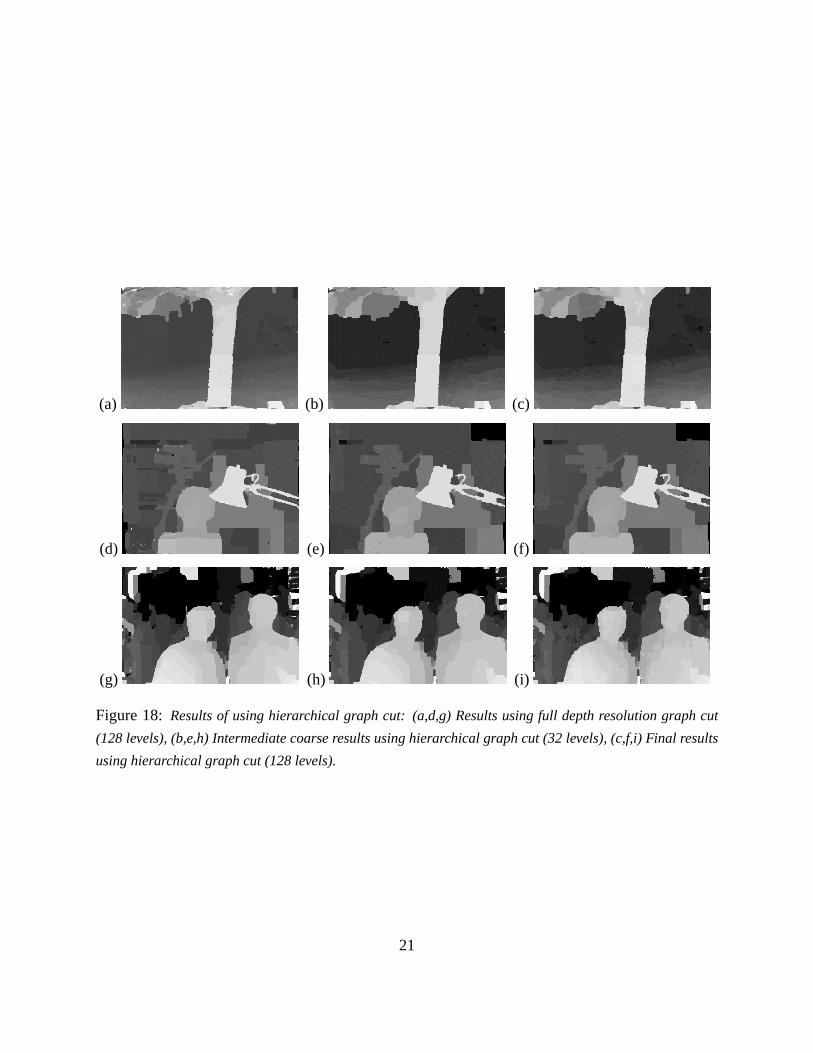
Results using the proposed hierarchical graph cut can be seen in Figure 18. In these sets of

experiments, we represent a coarse disparity level with four original disparity levels (reducing the

number of levels from 128 to 32 initially). As can be seen in Table 1, the duration of the graph cut

algorithm is reduced by a factor of between 4.0-4.4. The results obtained are comparable to those

with the full resolution graph cut. While there appears to be some degradation of quality in the

recovered depth maps (especially for the University of Tsukuba sequence), the visual reconstruction

remains very good (see Figures 20-22). The degradation is due to the early commitment of depth

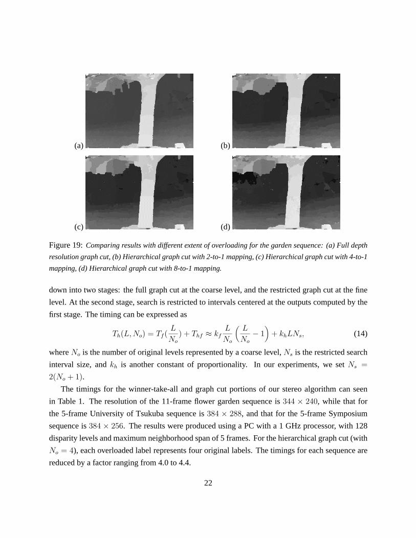
(as can be seen in Figure 18(b,e,h)). The result of using different extents of overloading can be seen

in Figure 19. Since the results look rather similar, the length of execution becomes a very important

consideration.

Since our graph cut algorithm consists of α − β swaps only [BVZ99], its complexity is propor-

tional to L(L − 1), where L is the number of labels, or disparities in our case. Hence the timing

for the full graph algorithm is

Tf (L) ≈ kfL(L − 1), (13)

where kf is a constant of proportionality. The timing for the hierarchical graph cut can be broken

20

(a) (b) (c)

(d) (e) (f)

(g) (h) (i)

Figure 18: Results of using hierarchical graph cut: (a,d,g) Results using full depth resolution graph cut

(128 levels), (b,e,h) Intermediate coarse results using hierarchical graph cut (32 levels), (c,f,i) Final results

using hierarchical graph cut (128 levels).

21

(a) (b)

(c) (d)

Figure 19: Comparing results with different extent of overloading for the garden sequence: (a) Full depth

resolution graph cut, (b) Hierarchical graph cut with 2-to-1 mapping, (c) Hierarchical graph cut with 4-to-1

mapping, (d) Hierarchical graph cut with 8-to-1 mapping.

down into two stages: the full graph cut at the coarse level, and the restricted graph cut at the fine

level. At the second stage, search is restricted to intervals centered at the outputs computed by the

first stage. The timing can be expressed as

Th(L, No) = Tf (L

No

) + Thf ≈ kfL

No

(L

No

− 1)

+ khLNs, (14)

where No is the number of original levels represented by a coarse level, Ns is the restricted search

interval size, and kh is another constant of proportionality. In our experiments, we set Ns =2(No + 1).

The timings for the winner-take-all and graph cut portions of our stereo algorithm can seen

in Table 1. The resolution of the 11-frame flower garden sequence is 344 × 240, while that for

the 5-frame University of Tsukuba sequence is 384 × 288, and that for the 5-frame Symposium

sequence is 384 × 256. The results were produced using a PC with a 1 GHz processor, with 128

disparity levels and maximum neighborhood span of 5 frames. For the hierarchical graph cut (with

No = 4), each overloaded label represents four original labels. The timings for each sequence are

reduced by a factor ranging from 4.0 to 4.4.

22

Operation Flower garden Tsukuba Symposium

Winner-take-all 2:19 2:20 2:27

Graph cut (full) 48:40 56:50 59:32

Graph cut (hierarchical) 11:03 14:05 13:24

Table 1: Timings for the three sequences (all in “minutes:seconds”). Note that in each case, the graph cut

algorithm is iterated four times for convergence.

A table comparing the timings for hierarchical graph cuts with different extents of overloading

is shown in Table 2. “L-to-1” refers to a coarse level representing L original levels. As can be

seen, increasing L does not necessarily reduce the duration of execution. We use average of the

University of Tsukuba and Symposium timings in Table 1 to estimate the ratio kh

kf, which yielded

2.249. We use this value to predict the timings for the flower garden sequence using (14); the

predicted values, which appear to be reasonable, are shown in Table 2.

Operation Actual Predicted

Graph cut (full) 48:40 —

Graph cut (hierarchical, 2-to-1) 18:17 17:15



Table 2: Graph cut timings for the flower garden sequence (all in “minutes:seconds”). Note that in each

case, the graph cut algorithm is iterated four times for convergence.

5 Discussion of Results

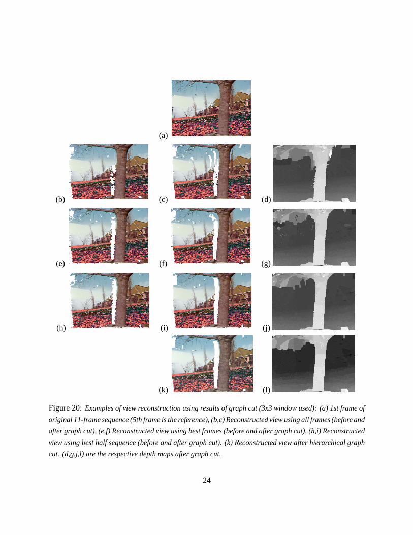
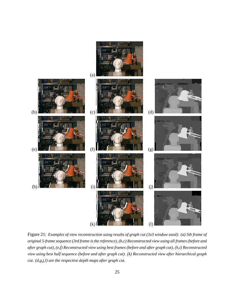
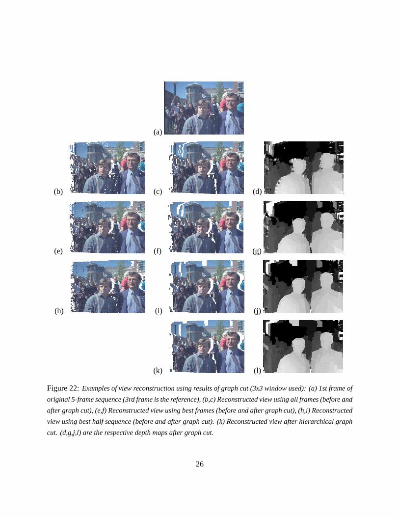
Figures 20-22 show view reconstruction results on our three image sequences. Note that the white

cracks observed in the reconstructed views are caused by transferring adjacent pixels with depth

discontinuities.

While our algorithm is targeted specifically towards multi-view stereo (with sequences of more

than two frames), it also produces reasonable results in two frame situations. The temporal selection

23

(a)

(b) (c) (d)

(e) (f) (g)

(h) (i) (j)

(k) (l)

Figure 20: Examples of view reconstruction using results of graph cut (3x3 window used): (a) 1st frame of

original 11-frame sequence (5th frame is the reference), (b,c) Reconstructed view using all frames (before and

after graph cut), (e,f) Reconstructed view using best frames (before and after graph cut), (h,i) Reconstructed

view using best half sequence (before and after graph cut). (k) Reconstructed view after hierarchical graph

cut. (d,g,j,l) are the respective depth maps after graph cut.

24

(a)

(b) (c) (d)

(e) (f) (g)

(h) (i) (j)

(k) (l)

Figure 21: Examples of view reconstruction using results of graph cut (3x3 window used): (a) 5th frame of

original 5-frame sequence (3rd frame is the reference), (b,c) Reconstructed view using all frames (before and




25

(a)

(b) (c) (d)

(e) (f) (g)

(h) (i) (j)

(k) (l)

Figure 22: Examples of view reconstruction using results of graph cut (3x3 window used): (a) 1st frame of

original 5-frame sequence (3rd frame is the reference), (b,c) Reconstructed view using all frames (before and




26

(a) (b)

(c) (d)

(e) (f)

(g) (h)

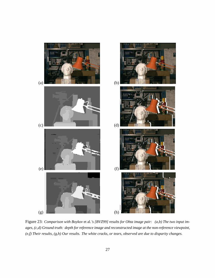
Figure 23: Comparison with Boykov et al.’s [BVZ99] results for Ohta image pair: (a,b) The two input im-

ages, (c,d) Ground truth: depth for reference image and reconstructed image at the non-reference viewpoint,

(e,f) Their results, (g,h) Our results. The white cracks, or tears, observed are due to disparity changes.

27

component is inoperative in this case. Our results compare favorably with Boykov et al.’s [BVZ99],

as can be seen in Figure 23.

To summarize our results, figures 7 and 9 show results using spatially shiftable windows op-

tionally combined with temporal selection, followed by a simple winner-take-all. The effects of

temporal selection are more dramatric than spatial shifting, and yield their biggest improvements

near depth discontinuities. Large textureless regions are still not recovered well.

Using incremental window sizes (Figures 10, 12, and 14) helps fill in more reasonable disparity

values in textureless regions, but still does not do that well in some areas such as the sky in the

Symposium sequence and the upper right corner of the U. Tsukuba sequence. Global optimization

techniques generally outperform this idea.

Adding an extra occluded pixel label to global optimization helps find regions that are visible

in only one image, such as the start and end frames for a multi-view sequence (Figure 15). This

should help the most when only a small number of frames is available (e.g., in classical two-frame

matching).

Finally, visibility reasoning is a good way to obtain better results near depth discontinuities

when the complete set of images is used as input to the data cost term (Figure 16). Reasoning about

which pixels are occluded allows us to iteratively re-compute a better data term. However, to our

surprise, this idea does not seem to help much if temporal selection has already been applied to

heuristically reject possibly occluded pixels, at least not on the data sets we have currently tried.

One possible direction for future work would be to take the visibility-based optimization for-

mulation (11) and to try to devise an algorithm that directly minimizes this function. Starting with a

solution that minimizes the original optimization formulation (i.e., ignoring the v(x, y, d, k) term),

we could optimize the complete function using a series of α − β swaps. Additional graph edge

links would have to be added between pixels in the current foreground (say α) layer and the pixels

in the current background (β) layer that they occlude to encode the change in visibility due to a

swap in the occluder’s status.

6 Conclusions

In this paper, we have presented several new ideas for improving the results of multi-view stereo

correspondence algorithms. Our particular emphasis has been on better dealing with pixels and

regions that are occluded in some images but not in others. Some of our ideas, such as temporal

28

selection, can be applied at the initial matching cost stage. Other ideas, such as outlier/invisible pixel

labeling and visibility reasoning, can be used to enhance the performance of global optimization

techniques such as graph cut algorithms. In addition, we have demonstrated that a hierarchical

graph cut algorithm can significantly reduce the execution time at a minimal loss in output quality.

Of all the ideas we have developed, using temporal selection (using only a subset of all frames

for computing the matching cost), followed by a regular graph cut global optimization, seems to

yield the best results for the least computational effort. It will be interesting to see how these ideas

generalize to other versions of multi-view stereo reconstruction, such as the extraction of multiple

layers and volumetric reconstruction techniques.

Acknowledgments

We would like to thank Ramin Zabih and Anandan for initial discussions on stereo matching.

References

[Arn83] R. D. Arnold. Automated stereo perception. Technical Report AIM-351, Artificial

Intelligence Laboratory, Stanford University, March 1983.

[BAHH92] J. R. Bergen, P. Anandan, K. J. Hanna, and R. Hingorani. Hierarchical model-based

motion estimation. In Second European Conference on Computer Vision (ECCV’92),

pages 237–252, Santa Margherita Liguere, Italy, May 1992. Springer-Verlag.

[Bar89] S. T. Barnard. Stochastic stereo matching over scale. International Journal of Com-

puter Vision, 3(1):17–32, 1989.

[Bel96] P. N. Belhumeur. A Bayesian-approach to binocular stereopsis. International Journal

of Computer Vision, 19(3):237–260, August 1996.

[BI99] A. F. Bobick and S. S. Intille. Large occlusion stereo. International Journal of Com-

puter Vision, 33(3):181–200, September 1999.

[BR96] M. J. Black and A. Rangarajan. On the unification of line processes, outlier rejec-

tion, and robust statistics with applications in early vision. International Journal of

Computer Vision, 19(1):57–91, 1996.

29

[BSA98] S. Baker, R. Szeliski, and P. Anandan. A layered approach to stereo reconstruction.

In IEEE Computer Society Conference on Computer Vision and Pattern Recognition

(CVPR’98), pages 434–441, Santa Barbara, June 1998.

[BT98] S. Birchfield and C. Tomasi. A pixel dissimilarity measure that is insensitive to im-

age sampling. IEEE Transactions on Pattern Analysis and Machine Intelligence,

20(4):401–406, April 1998.

[BT99] S. Birchfield and C. Tomasi. Multiway cut for stereo and motion with slanted surfaces.

In Seventh International Conference on Computer Vision (ICCV’99), pages 489–495,

Kerkyra, Greece, September 1999.

[BVZ99] Y. Boykov, O. Veksler, and R. Zabih. Fast approximate energy minimization via graph

cuts. In Seventh International Conference on Computer Vision (ICCV’99), pages 377–

384, Kerkyra, Greece, September 1999.

[CB90] P. B. Chou and C. M. Brown. The theory and practice of Bayesian image labeling.

International Journal of Computer Vision, 4(3):185–210, June 1990.

[Col96] R. T. Collins. A space-sweep approach to true multi-image matching. In IEEE Com-

puter Society Conference on Computer Vision and Pattern Recognition (CVPR’96),

pages 358–363, San Francisco, California, June 1996.

[DA89] U. R. Dhond and J. K. Aggarwal. Structure from stereo—a review. IEEE Transactions

on Systems, Man, and Cybernetics, 19(6):1489–1510, November/December 1989.

[GG84] S. Geman and D. Geman. Stochastic relaxation, Gibbs distribution, and the Bayesian

restoration of images. IEEE Transactions on Pattern Analysis and Machine Intelli-

gence, PAMI-6(6):721–741, November 1984.

[GLY92] D. Geiger, B. Ladendorf, andA.Yuille. Occlusions and binocular stereo. In Second Eu-

ropean Conference on Computer Vision (ECCV’92), pages 425–433, Santa Margherita

Liguere, Italy, May 1992. Springer-Verlag.

[HA86] W. Hoff and N. Ahuja. Surfaces from stereo. In Eighth International Conference on

Pattern Recognition (ICPR’86), pages 516–518, Paris, France, October 1986. IEEE

Computer Society Press.

30

[Han91] K. J. Hanna. Direct multi-resolution estimation of ego-motion and structure from

motion. In IEEE Workshop on Visual Motion, pages 156–162, Princeton, New Jersey,

October 1991. IEEE Computer Society Press.

[IG98] H. Ishikawa and D. Geiger. Occlusions, discontinuities, and epipolar lines in stereo. In

Fifth European Conference on Computer Vision (ECCV’98), pages 232–248, Freiburg,

Germany, June 1998. Springer-Verlag.

[JBJ96] S. X. Ju, M. J. Black, and A. D. Jepson. Skin and bones: Multi-layer, locally affine,

optical flow and regularization with transparency. In IEEE Computer Society Confer-

ence on Computer Vision and Pattern Recognition (CVPR’96), pages 307–314, San

Francisco, California, June 1996.

[KS99] K. N. Kutulakos and S. M. Seitz. A theory of shape by space carving. In Seventh

International Conference on Computer Vision (ICCV’99), pages 307–314, Kerkyra,

Greece, September 1999.

[KWZK95] S. B. Kang, J. Webb, L. Zitnick, and T. Kanade. A multibaseline stereo system with

active illumination and real-time image acquisition. In Fifth International Conference

on Computer Vision (ICCV’95), pages 88–93, Cambridge, Massachusetts, June 1995.

[KZ01] V. Kolmogorov and R. Zabih. Computing visual correspondence with occlusions using

graph cuts. In Eighth International Conference on Computer Vision (ICCV 2001),

volume II, pages 508–515, Vancouver, Canada, July 2001.

[LK81] B. D. Lucas and T. Kanade. An iterative image registration technique with an ap-

plication in stereo vision. In Seventh International Joint Conference on Artificial

Intelligence (IJCAI-81), pages 674–679, Vancouver, 1981.

[MMP87] J. Marroquin, S. Mitter, and T. Poggio. Probabilistic solution of ill-posed problems in

computational vision. Journal of the American Statistical Association, 82(397):76–89,

March 1987.

[MP79] D. C. Marr and T. Poggio. A computational theory of human stereo vision. Proceedings

of the Royal Society of London, B 204:301–328, 1979.

31

[MSK89] L. H. Matthies, R. Szeliski, and T. Kanade. Kalman filter-based algorithms for es-

timating depth from image sequences. International Journal of Computer Vision,

3:209–236, 1989.

[NMSO96] Y. Nakamura, T. Matsuura, K. Satoh, andY. Ohta. Occlusion detectable stereo - occlu-

sion patterns in camera matrix. In IEEE Computer Society Conference on Computer

Vision and Pattern Recognition (CVPR’96), pages 371–378, San Francisco, California,

June 1996.

[OK85] Y. Ohta and T. Kanade. Stereo by intra- and inter-scanline search using dynamic pro-

gramming. IEEE Transactions on Pattern Analysis and Machine Intelligence, PAMI-

7(2):139–154, March 1985.

[OK92] M. Okutomi and T. Kanade. A locally adaptive window for signal matching. Interna-

tional Journal of Computer Vision, 7(2):143–162, April 1992.

[OK93] M. Okutomi and T. Kanade. A multiple baseline stereo. IEEE Transactions on Pattern

Analysis and Machine Intelligence, 15(4):353–363, April 1993.

[PTK85] T. Poggio, V. Torre, and C. Koch. Computational vision and regularization theory.

Nature, 317(6035):314–319, 26 September 1985.

[RC98] S. Roy and I. J. Cox. A maximum-flow formulation of the N-camera stereo correspon-

dence problem. In Sixth International Conference on Computer Vision (ICCV’98),

pages 492–499, Bombay, January 1998.

[SAA00] R. Szeliski, S.Avidan, and P.Anandan. Layer extraction from multiple images contain-

ing reflections and transparency. In IEEE Computer Society Conference on Computer

Vision and Pattern Recognition (CVPR’2000), volume 1, pages 246–253, Hilton Head

Island, June 2000.

[SC94] R. Szeliski and J. Coughlan. Hierarchical spline-based image registration. In

IEEE Computer Society Conference on Computer Vision and Pattern Recognition

(CVPR’94), pages 194–201, Seattle, Washington, June 1994. IEEE Computer Society.

[SC97] R. Szeliski and J. Coughlan. Hierarchical spline-based image registration. Interna-

tional Journal of Computer Vision, 22(3):199–218, March/April 1997.

32

[SD97] S. M. Seitz and C. M. Dyer. Photorealistic scene reconstrcution by voxel coloring.

In IEEE Computer Society Conference on Computer Vision and Pattern Recognition

(CVPR’97), pages 1067–1073, San Juan, Puerto Rico, June 1997.

[SG99] R. Szeliski and P. Golland. Stereo matching with transparency and matting. Interna-

tional Journal of Computer Vision, 32(1):45–61, August 1999. Special Issue for Marr

Prize papers.

[SHK00] S. Sun, D. Haynor, andY. Kim. Motion estimation based on optical flow with adaptive

gradients. In International Conference on Image Processing (ICIP-2000), volume I,

pages 852–855, Vancouver, September 2000.

[SS98] D. Scharstein and R. Szeliski. Stereo matching with nonlinear diffusion. International

Journal of Computer Vision, 28(2):155–174, July 1998.

[ST94] J. Shi and C. Tomasi. Good features to track. In IEEE Computer Society Conference

on Computer Vision and Pattern Recognition (CVPR’94), pages 593–600, Seattle,

Washington, June 1994. IEEE Computer Society.

[SZ99] R. Szeliski and R. Zabih. An experimental comparison of stereo algorithms. In In-

ternational Workshop on Vision Algorithms, pages 1–19, Kerkyra, Greece, September

1999. Springer.

[Sze99] R. Szeliski. A multi-view approach to motion and stereo. In IEEE Computer Society

Conference on Computer Vision and Pattern Recognition (CVPR’99), volume 1, pages

157–163, Fort Collins, June 1999.

[Ter86] D. Terzopoulos. Regularization of inverse visual problems involving discontinuities.

IEEE Transactions on Pattern Analysis and Machine Intelligence, PAMI-8(4):413–

424, July 1986.

[TSK01] H. Tao, H.S. Sawhney, and R. Kumar. A global matching framework for stereo compu-

tation. In Eighth International Conference on Computer Vision (ICCV 2001), volume I,

pages 532–539, Vancouver, Canada, July 2001.

[Vek99] O. Veksler. Efficient Graph-based Energy Minimization Methods in Computer Vision.

PhD thesis, Cornell University, July 1999.

33

[WA93] J. Y. A. Wang and E. H. Adelson. Layered representation for motion analysis. In

IEEE Computer Society Conference on Computer Vision and Pattern Recognition

(CVPR’93), pages 361–366, New York, New York, June 1993.

[Wei97] Y. Weiss. Smoothness in layers: Motion segmentation using nonparametric mixture

estimation. In IEEE Computer Society Conference on Computer Vision and Pattern

Recognition (CVPR’97), pages 520–526, San Juan, Puerto Rico, June 1997.

[ZK00] C. L. Zitnick and T. Kanade. A cooperative algorithm for stereo matching and oc-

clusion detection. IEEE Transactions on Pattern Analysis and Machine Intelligence,

22(7):675–684, July 2000.

[ZS00] Z. Zhang and Y. Shan. A progressive scheme for stereo matching. In M. Pollefeys

et al., editors, Second European Workshop on 3D Structure from Multiple Images of

Large-Scale Environments (SMILE 2000), pages 68–85, Dublin, Ireland, July 2000.

34

handling occlusions in dense multi-view stereo · handling occlusions in dense multi-view stereo...

Documents