hardware realization of a transform domain …
TRANSCRIPT

HARDWARE REALIZATION OF A TRANSFORM
DOMAIN COMMUNICATION SYSTEM
THESIS
Marshall E. Haker, Captain, USAF
AFIT/GE/ENG/07-10
DEPARTMENT OF THE AIR FORCEAIR UNIVERSITY
AIR FORCE INSTITUTE OF TECHNOLOGYWright-Patterson Air Force Base, Ohio
APPROVED FOR PUBLIC RELEASE; DISTRIBUTION UNLIMITED

The views expressed in this thesis are those of the author and do not reflect the official policy or position of the United States Air Force, Department of Defense, or the United States Government.

AFIT/GE/ENG/07-10
HARDWARE REALIZATION OF A TRANSFORM DOMAIN COMMUNICATION SYSTEM
THESIS
Presented to the Faculty
Department of Electrical and Computer Engineering
Graduate School of Engineering and Management
Air Force Institute of Technology
Air University
Air Education and Training Command
In Partial Fulfillment of the Requirements for the
Degree of Master of Science in Electrical Engineering
Marshall E. Haker, BS
Captain, USAF
March 2007
APPROVED FOR PUBLIC RELEASE; DISTRIBUTION UNLIMITED.

AFIT/GE/ENG/07-10
HARDWARE REALIZATION OF A TRANSFORMDOMAIN COMMUNICATION SYSTEM
Marshall E. Haker, BSCaptain, USAF
Approved:
/signed/ ____________________________________
Richard K. Martin (Chairman) date
/signed/ ____________________________________
Michael A. Temple (Member) date
/signed/____________________________________
Stewart L. DeVilbiss (Member) date

AFIT/GE/ENG/07-10
Abstract
The purpose of this research was to implement a Transform Domain Communication
System (TDCS) in hardware and compare experimental bit error performance with results
published in literature. The intent is to demonstrate the effectiveness or ineffectiveness
of a TDCS in communicating binary data across a real channel. In this case, an acoustic
channel that is laden with narrowband interference was considered. A TDCS user pair
was constructed to validate the proposed design using Matlab® to control a PC sound
card. The proposed TDCS design used the Bartlett method of spectrum estimation, the
spectral notching algorithm found in TDCS literature, quadrature phase shift keying, and
minimum mean square error transverse equalization to mitigate the effects of noise and
intersymbol interference. Water-filling was evaluated as an alternative to spectral
notching for performing waveform design and is shown to perform equivalently.
Validated software was migrated to code suitable for use onboard a Digital Signal
Processor Starter Kit (DSK). Two DSK boards were used, one for transmission and
reception, and bit error performance results were obtained. Bit error analysis reveals that
the TDCS hardware performs approximately the same as literature suggests.
iv

AFIT/GE/ENG/07-10
To my Son and Daughter,
my two best reasons for getting out of bed in the morning
v

Acknowledgments
I would like to express my sincere gratitude to my faculty advisor, Dr. Richard
Martin, who steered me through this research process, and who never left me feeling
stupid for asking something really stupid. Thanks also to my thesis committee members,
Dr. Michael Temple and Dr. Stewart Devilbiss, for taking me on as an occasional
schedule-killer in the impromptu office visit. Further gratitude goes out to my research
sponsor, Mr. Vasu Chakravarthy of the Air Force Research Laboratory Sensors
Directorate, who didn't blink when the risks in trying to “do it” in hardware came up.
Of course, thanks to my family, my parents and brothers, and my in-laws (have
in-laws ever been acknowledged before?).
There's a long list of people who have helped me get here, some of the most
notable being Lt Col Gary Ashworth, Lt Col Earl Culek, Major George Mellen, Lt and
Mrs. Bill Keichel, Lt and Mrs. Matt Williams, Dr. Lee Potter, Mr. Glen Hosford, Mr.
Ralph Petrosky, Mr. Tom Ramsey, Col Dan Lombardi, and the Technical Gladiators:
Mr. Dan Mitchell, Dr. Kristian Olivero, Mr. Jimmy Byus, and certainly Mr. Jess Phillips.
Finally, I'm most thankful of all to my wife, who succeeded in keeping our
children giggling outside while their dad was holed up in the dungeon. Next time it's
your turn, as you've been waiting to “do something great.” I think you already have.
Marshall E. Haker
vi
Table of Contents
PageAbstract ....................................................................................................................... iv
Dedication .....................................................................................................................v
Acknowledgments ....................................................................................................... vi
Table of Contents .......................................................................................................vii
List of Figures .............................................................................................................. ix
I. Introduction ............................................................................................................11.1. Background.................................................................................................... 11.2. Problem Statement......................................................................................... 21.3. Goals...............................................................................................................21.4. Scope.............................................................................................................. 31.5. Assumptions................................................................................................... 31.6. Methodology...................................................................................................41.7. Materials.........................................................................................................41.8. Overview........................................................................................................ 5
II. Literature Review................................................................................................... 72.1. Transform Domain Communication System (TDCS) History.......................72.2. An Aside on Hadamard Multiplication and the Hadamard Product............ 122.3. Current State of the TDCS Architecture...................................................... 13
2.3.1. Estimate Spectrum.............................................................................132.3.2. Spectrum Magnitude......................................................................... 152.3.3. Pseudorandom Phase......................................................................... 162.3.4. Scaling............................................................................................... 172.3.5. IDFT.................................................................................................. 172.3.6. Buffer.................................................................................................182.3.7. Modulation/Transmission..................................................................192.3.8. Receiver Architecture at Large..........................................................19
2.4. Synchronization of Received TDCS Signals................................................202.5. Spectrally Modulated, Spectrally Encoded Signaling..................................212.6. Equalization of Received TDCS Signals......................................................282.7. Coexistence.................................................................................................. 302.8. Coexistence and the Pursuit of LPI/LPD Communications......................... 34
2.8.1. Water-filling...................................................................................... 352.9. Digital Signal Processing Hardware and Programming...............................38
vii

PageIII. TDCS Architecture Implementation.................................................................. 40
3.1. Transmitter................................................................................................403.1.1. Spectrum Estimation.....................................................................403.1.2. Spectrum Magnitude Calculation................................................. 443.1.3. Pseudorandom Phase Generation................................................. 473.1.4. Data (Waveform) Modulation...................................................... 493.1.5. Scaling.......................................................................................... 493.1.6. IDFT............................................................................................. 503.1.7. Buffer............................................................................................523.1.8. Modulation (Bits-to-Symbols)/Transmission............................... 53
3.2. Acquisition of Received Signals...............................................................533.3. Synchronization of Received Signals....................................................... 533.4. Reception and Demodulation of Received Signals.................................. 553.5. Equalizing Received Signals.................................................................... 573.6. Computing SNR and Eb/N0.......................................................................................................................... 60
IV. Spectral Notching Versus Water-filling.............................................................634.1. TDCS Performance: Spectral Notching vs. Water-filling....................... 654.2. Coexistence Performance: Spectral Notching vs. Water-filling..............664.3. Spectrum Estimate Mismatch: Spectral Notching vs. Water-filling...... 674.4. Interpretation of Simulation Results.........................................................694.5. Summary...................................................................................................70
V. Hardware Implementation Results..................................................................... 715.1. No Spectral Notching with No Interference Added to Environment....... 735.2. No Spectral Notching with Interference Added to Environment............. 755.3. Spectral Notching with Interference Added to Environment................... 765.4. Spectral Notching with No Interference Added to Environment............. 795.5. Comparing Unequalized and Equalized Bit Error Performance Results..815.6. Summary...................................................................................................81
VI. Conclusion..........................................................................................................846.1. Recommendations for Further Research.................................................. 85
Bibliography................................................................................................................ 86
Vita...............................................................................................................................89
viii

List of Figures
Figure Page
1. TDCS Transmitter Block Diagram.......................................................................14
2. Bartlett Method of Spectrum Estimation..............................................................15
3. Spectrum Magnitude Block Functionality............................................................16
4. Pseudorandom Phase Vector Generation..............................................................17
5. TDCS Receiver Block Diagram........................................................................... 20
6. PSD of Two Narrowband QPSK Interferers in Noiseless Channel......................36
7. Spectrum Estimate (via Bartlett Method) ofInterferers Theoretically Obtained by Transmitter............................................... 36
8. PSD of Proposed Waveform Generated for Transmission via Water-filling....... 37
9. Spectrum Estimate of Water-filled TDCSCommunications Waveform Coexisting with Interferers.....................................37
10. Portion of Flattened Spectrum Immediately Aroundthe Higher Powered of the Two Narrowband Interferers..................................... 38
11. TDCS Transmitter Block Diagram Incorporating SMSE Notation......................41
12. Single Realization of Bartlett Spectrum Estimation Output forTypically Noisy Channel with Tone Interferer Present at 2.000 kHz.................. 45
13. Single Realization of Spectrum Magnitude Output for TypicallyNoisy Channel with Tone Interferer Present at 2.000 kHz...................................47
14. Single Realization of Pseudorandom CodeVector c[m] for Use in Spectral Encoding............................................................50
15. Time-domain Communications Signal Waveforms for TD-QPSK Signaling..... 52
16. TD-QPSK Signal Space and Decision Boundaries for Hardware Implementation54
16. TD-QPSK Signal Space and DecisionBoundaries for Hardware Implementation........................................................... 57
17. TDCS Receiver Block Diagram Incorporating SMSE Notation.......................... 56
ix

Figure Page
18. Demodulated TD-QPSK Symbol Constellation of 375 DemodulatedSymbols at Eb/N0 = 9.85 dB Communicated in a Single One-Second Burst........57
19. Equalized TD-QPSK Symbol Constellation of 375 DemodulatedSymbols at Eb/N0 = 9.85 dB in Same One Second Burst Used in Figure 18........ 60
20. Bit Error Performance for TDCS usingSpectral Notching and Water-filling.....................................................................66
21. Bit Error Performance for QPSK User Coexistingwith TDCS User (No Interference Present)..........................................................67
22. Bit Error Performance for Spectrally Mismatched TDCS User Pair....................69
23. Photograph Illustrating Equipment PositioningDuring All DSK-based Experiments.................................................................... 72
24. Unequalized Bit Error Performance Curve of HardwareRealization. No Spectral Notching in an EnvironmentWithout Additional Narrowband Interference...................................................... 74
25. Equalized Bit Error Performance Curve of HardwareRealization. No Spectral Notching in an EnvironmentWithout Additional Narrowband Interference...................................................... 74
26. Unequalized Bit Error Performance Curve of HardwareRealization. No Spectral Notching in anEnvironment with Additional Narrowband Interference...................................... 76
27. Equalized Bit Error Performance Curve of HardwareRealization. No Spectral Notching in anEnvironment with Additional Narrowband Interference...................................... 76
28. Unequalized Bit Error Performance Curve of HardwareRealization using Spectral Notching in an Environmentwith Additional Narrowband Interference............................................................ 78
29. Equalized Bit Error Performance Curve of HardwareRealization using Spectral Notching in an Environmentwith Additional Narrowband Interference............................................................ 78
x

Figure Page
30. Unequalized Bit Error Performance Curve of HardwareRealization using Spectral Notching in an Environment Without Additional Narrowband Interference...................................................... 80
31. Equalized Bit Error Performance Curve of HardwareRealization using Spectral Notching in an Environment Without Additional Narrowband Interference...................................................... 80
32. Comparison of Unequalized and Equalized Bit ErrorPerformance in Scenario with No Spectral Notching and No Narrowband Interference Added to the Environment.....................................82
33. Comparison of Unequalized and Equalized Bit ErrorPerformance in Scenario with No Spectral Notchingand with Additional Narrowband Interference..................................................... 82
34. Comparison of Unequalized and Equalized Bit ErrorPerformance in Scenario with Spectral Notchingand with Additional Narrowband Interference..................................................... 83
35. Comparison of Unequalized and Equalized Bit ErrorPerformance in Scenario with Spectral Notching andNo Narrowband Interference Added to the Environment.....................................83
xi

HARDWARE REALIZATION OF A
TRANSFORM DOMAIN COMMUNICATION SYSTEM
I. Introduction
1.1. Background
Transform Domain Communications System (TDCS) research has been
conducted for over a decade in a joint effort between the Air Force Institute of
Technology (AFIT) and the Air Force Research Laboratory (AFRL) Sensors Directorate
[1]-[8]. This research was spurred by the notion that it may be possible to communicate
using digital signaling while both avoiding interfering signals in the RF spectrum
bandpass of interest [9] and ensuring a low probability of detection, intercept, and/or
exploitation (LPD/LPI/LPE) [8, 10]. Over the course of the last decade, this research has
involved efforts to determine the feasibility and effectiveness of a TDCS in signal
acquisition and synchronization, application in a multiple access network, and the impact
of multipath and intersymbol interference on TDCS signaling. The intrinsic capability of
a TDCS to avoid interference has been studied as well. While this research has been
published and reported in venues such as the IEEE Communications Magazine [8], and
has even at least partially motivated the development of a digital communications
signaling framework [11], there has never been a formal attempt to implement a TDCS in
hardware. Rather, all previous research has involved simulating TDCS signaling between
a user pair in various environments. The intent of this research was to take the next
1

logical step in TDCS research: the realization and study of a TDCS hardware
implementation.
1.2. Problem Statement
There has never been a formal attempt to implement the TDCS architecture in
hardware. To do this, the design and construction of the traditional transmitter-receiver
user pair, as well as functions such as synchronization and equalization, must be
considered. Furthermore, several different design decisions must be made in order to fill
gaps between a communications transceiver or network model used in simulations and a
realized, functional hardware implementation. This thesis represents the first attempt at
realizing a TDCS in hardware, with the perspective taken that this realization is intended
to serve as a proof-of-concept. This being the case, the TDCS hardware realization uses
an acoustic channel that is intended to serve as a scale model of an RF channel, complete
with noise and interference.
1.3. Goals
The overarching goals of this research effort are:
1. To compare the bit error performance of a TDCS hardware implementation with
the expected values expressed in literature.
2. To assess the capability of a digital signal processor (DSP) in hosting either a
TDCS transmitter or receiver.
3. To examine the utility of applying a method of communications waveform
sculpting, other than the previously used spectral notching technique [1-8], such
as water-filling, through the use of Matlab®-based simulations.
2
1.4. Scope
This research is restricted to examining an implementation of a TDCS in
hardware using transform domain quadrature phase shift keying (TD-QPSK) and a
minimum mean square error (MMSE) equalizer in an undefined channel. This channel is
assumed to consist of additive white Gaussian noise (AWGN), various interfering signals
(both controlled and uncontrolled), and intersymbol interference due to multipath
propagation effects. Given the channel at hand, the ability of a TDCS hardware user pair
to conduct trained channel estimation via an MMSE equalizer is intrinsically studied.
There is no attempt made to implement other modulation schemes, such as cyclic shift
keying (CSK) or any form of M-ary PSK other than QPSK, nor is there an attempt made
to optimize the equalization or synchronization algorithms, either in terms of efficiency or
effectiveness. There is no attempt to compare the performance of a TDCS user pair with
simulated results in terms of the ability of the TDCS receiver to acquire a TDCS
transmission. Synchronization is and must be performed in order to process received
communications symbols, but the effectiveness of synchronization is not explicitly
studied.
1.5. Assumptions
The following assumptions are made in this research:
1. The MMSE equalizer implemented in the user pair is assumed to mitigate all
residual effects due to multipath, so the assumption is made that the matched filter
correlation process used to demodulate received TDCS signals is optimal.
3

2. The hardware-implemented TDCS user pair is assumed to be perfectly
synchronized.
1.6. Methodology
TDCS software simulations are used to initially validate the TDCS algorithm used
in the hardware user pair. Once this validation is complete, the TDCS software is
implemented in a hybrid software/hardware PC-based prototyping platform to conduct
validation of the software in an acoustic channel consisting of a common office or home
environment. This hybrid prototyping platform consisting of a single PC with multiple
instances of Matlab® running. One instance of Matlab® code is written to generate
and transmit a TDCS signal through an acoustic channel, using PC speakers. The other
instance of code is written for receiving the TDCS signal using a PC microphone and for
processing the received signal. Finally, the TDCS software is migrated to a format
suitable for a DSP, the software is transferred to the DSP cards, and experiments are
conducted. These experiments, conducted using four scenarios, result in calculation of
empirically-obtained bit error rates, which are then compared with the analytic QPSK
curve, as well as bit error rates from other scenarios.
1.7. Materials
All simulations and the initial software/hardware hybrid prototyping is performed
using Matlab® Student Version 7.0 (R14). Simulations and prototyping are run on
stand-alone PCs, including a Dell Pentium-based laptop and a Dell Pentium-based
desktop computer. The DSP-based TDCS hardware user pair is implemented using two
Spectrum Digital TMS320C6416 (1 GHz) DSP Starter Kits (DSK). The DSK uses the
4

Texas Instruments TMS3206416 fixed point DSP operating at 1 GHz. The DSK is
programmed using the Texas Instruments Code Composer Studio Version 3.1, included
with the DSK. Code Composer Studio uses C-based scripts to control the DSK. Two
Cyber Acoustics AC-54 PC desktop microphones, one for each DSK, are used to perform
signal reception and environmental sampling for spectrum estimation. Acoustic signal
transmission is performed using one Labtec LCS-1070 PC desktop speaker. Narrowband
interfering signals are generated using Matlab® to control two Labtec LCS-1050 PC
desktop speakers.
1.8. Overview
This thesis is organized into six chapters. Chapter II, the Literature Review,
provides a historical perspective on TDCS and discusses literature on several topics of
interest used to make the design decisions involved in this research effort. These topics
include discussion of the framework for spectrally modulated, spectrally encoded (SMSE)
digital communications; interference avoidance and its association with coexistence and
LPD communication; how waveform design, or “sculpting,” thus waveform agility,
enables interference avoidance; equalization of received digital communications signals;
and background into the DSK implementation. Chapter III outlines the architecture of the
TDCS system being implemented, and includes several illustrations to convey graphically
some of the ideas behind the theory. Chapter III also discusses the tradeoffs involved in
the design used to obtain results with the hardware user pair. Chapter IV provides some
simulation results used when studying water-filling as an alternative to spectral notching
when performing TDCS communications symbol waveform design. Water-filling is
5

studied because literature indicates that water-filling may more optimally fit within the
managed spectrum than spectral notching. Simulated bit error performance curves
resulting from this research are provided in Chapter IV. Chapter V provides the bit error
results obtained with DSK hardware. These results are then compared with the analytic
QPSK bit error performance curve and with previous results in TDCS literature. Finally,
Chapter VI contains the research conclusion and provides some recommendations for
future TDCS research.
6

II. Literature Review
2.1. Transform Domain Communication System (TDCS) History
There have been several theses written by graduate students at AFIT on various
aspects of TDCS. In all cases, the research approach in studying TDCS consists of,
unless stated otherwise in the context of a specific research effort, conducting a literature
review on digital communications enterprise-wide approaches to resolving the obstacles
in fielding a TDCS user pair or network, as well as obviously all literature on previous
TDCS research efforts. Once the literature review is completed, design approaches are
integrated into the TDCS transceiver architecture. The integration into the TDCS design
model of the algorithm in question (such as Roberts' integration of synchronization
algorithms into the TDCS architecture [3], or Klein or Lee's integration of wavelet-
domain processing in the TDCS spectrum estimation algorithm [4, 5], for example) is
then performed using Matlab®, and the results obtained via simulations using the
Matlab® models are then compared with expected results from literature.
Initially, the TDCS research line was initiated with AFRL-contracted efforts that
led to a technical report [9] and the filing of a patent [10]. These technical reports were
then used as foundational works by Radcliffe in his groundbreaking proposal of the
TDCS, which is outlined in his thesis [1]. The original block diagram for the TDCS
transmitter and receiver proposed by Radcliffe still largely stand as written [1]. Radcliffe
demonstrated that in an AWGN channel with interference of varying types (tone, swept
tone, limited instances of partial band, and interference across the bandwidth of the
TDCS signaling) present, the TDCS interference avoidance algorithm demonstrates better
7

performance (at a signal energy to channel noise ratio (Eb/N0) of 4 dB, antipodal signaling
exhibited 12.7 dB improvement, while binary orthogonal modulation exhibited a 6.8 dB
improvement [1]) than direct sequence spread spectrum. Radcliffe's research is limited to
cases involving a single stationary transmitter and a single stationary receiver operating as
a user pair that shares a channel that contains only AWGN and various types of
interfering signals (thus no multipath) [1]. Radcliffe assumed that the TDCS user pair
operates with a flat frequency magnitude response over the bandwidth of interest, that the
propagation delay between transmitter and receiver is zero, that synchronization between
the transmitter and receiver is perfect, and that there is a perfect consensus reached
between the transmitter and receiver in all decisions on which areas of the spectrum are
impacted by interference, thus which parts of the spectrum to avoid [1]. Radcliffe
provided the TDCS architecture on which all other AFIT and AFRL research efforts are
based.
Swackhammer followed up Radcliffe's work by studying the potential for multiple
TDCS users working in a multiple access network, and found that code division multiple
access (CDMA) algorithms could be used to achieve multiple access capability [2]. This
CDMA coding is integrated into the TDCS waveform design algorithm, and an
asynchronous multiple access network of up to eight channels is simulated. The bit error
performance of a single user pair within this network is studied for Eb/N0 ranging from 0
to 9 dB [2]. Swackhammer then compared simulation results with bit error performance
estimates using cross-correlation calculations and concluded that TDCS signaling could
be employed practically in a multiple access network [2]. Swackhammer's research is
8

limited to cases involving up to eight stationary transmitters and up to eight stationary
receivers operating as user pairs that simultaneously share a channel containing only
AWGN and multiple access interference created by user pairs within the network (thus no
multipath or interfering signals not associated with users in the multiple access network)
[2]. Swackhammer assumed that the TDCS user pair operates with a flat frequency
magnitude response over the bandwidth of interest, that the propagation delay between
transmitter and receiver is zero, that synchronization between the transmitter and receiver
is perfect, and that there is a perfect consensus reached between the transmitter and
receiver in all decisions on which areas of the spectrum are impacted by interference [2].
Swackhammer's work justifies further study into TDCS in a multiple access environment,
and perhaps the physical implementation of TDCS into a network.
Roberts performed study into synchronization of a TDCS system, and found that a
TDCS user pair can indeed be synchronized when signaling in the presence of
interference [3]. Roberts studied several different acquisition and synchronization
protocols, integrated them into the TDCS architecture, and found that a Direct Time
Correlation (DTC) algorithm can be executed to provide both peak and threshold
detection [3]. Peak and threshold detection enable synchronization and acquisition,
respectively. Roberts examined the use of German's technique [9], and found that
specifically for threshold detection above -12 dB signal-to-noise ratio (SNR), German's
technique performs better than DTC [3]. Roberts's research is limited to cases involving
a single stationary transmitter and a single stationary receiver operating as a user pair
sharing channel containing only AWGN and 10% partial band interference (thus no
9

multipath) [3]. Roberts assumed that the TDCS user pair operates with a flat frequency
magnitude response over the bandwidth of interest, that the propagation delay between
transmitter and receiver is zero, and that there is a perfect consensus reached between the
transmitter and receiver in all decisions on which areas of the spectrum are impacted by
interference [3]. Roberts' research into the acquisition and synchronization of a TDCS is
used in the various design decisions made in implementing TDCS in hardware, such as
the use of DTC for symbol synchronization. Roberts goes much further to contribute to
TDCS research in offering a framework for SMSE signaling (in which TDCS is
included), but discussion into this subject is reserved for Section 2.5.
Klein integrated wavelet processing techniques into the TDCS framework,
yielding a Wavelet Domain Communication System (WDCS) [4]. Lee contributed
further by integrating the use of packets into the WDCS construct [5]. The work of
neither Klein nor Lee has been used in this research effort, so no further discussion into
WDCS is included here.
Radcliffe, Swackhammer, and Roberts all used antipodal and CSK modulation to
communicate bit values [1-3]. The use of CSK enabled M-ary (as opposed to binary)
signaling, but exhibits less spectral efficiency than what can be achieved by other means
[6]. Nunez researched the integration of PSK modulation into TDCS signaling, to answer
this shortcoming [6]. His design involves implementation of transform domain PSK
modulation in the time-domain after performing a discrete Fourier transform on TDCS
frequency-domain waveforms. This is done through the use of fixed phase rotations of
the pseudorandom phase vector used to spectrally encode the TDCS communications
10

symbols [6]. Section 2.3.5 goes further to discuss the specifics of how PSK modulation
is implemented in TDCS, and Section 2.5 presents modulation in the SMSE framework.
Nunez's results demonstrate that TD-QPSK mitigates interference in an AWGN channel
with a bit error performance roughly equivalent to spectrally unencoded PSK signaling
with no interference present [6]. It is expected that applying the spectral notching
algorithm to experiments that use TD-QPSK will yield the same result. Nunez's work
also yields the finding that, in the presence of narrowband interference and at bit error
rates of less than 10-3, the use of spectral notching yields a gain in Eb/N0 of greater than 1
dB, and that at bit error rates of less than 10-2, there should be an appreciable
improvement in bit error performance [6]. Nunez's research is limited to cases involving
up to 32 stationary transmitters and up to 32 stationary receivers operating as user pairs
simultaneously sharing a channel containing AWGN, narrowband interference, and
multiple access interference (thus no multipath) [6]. Nunez assumed that the TDCS user
pair operates with a flat frequency magnitude response over the bandwidth of interest,
that the propagation delay between transmitter and receiver is zero, that synchronization
between the transmitter and receiver is perfect, and that there is a perfect consensus
reached between the transmitter and receiver in all decisions on which areas of the
spectrum are impacted by interference [6]. Nunez's work is used directly in
implementing TDCS in hardware, as TD-QPSK is used exclusively in all waveform
designs.
In the latest of the AFIT research efforts addressing TDCS as the explicit focus,
Gaona was the first to study TDCS performance in the presence of multipath interference
11

[7]. He integrated a RAKE receiver into the TDCS architecture, and found that TDCS
intrinsically mitigates multipath effects [7]. A RAKE receiver exploits multipath
propagation to coherently reconstruct a communications signal by processing the multiple
received signals resulting from the various propagation paths [16]. Gaona's research is
limited to cases involving a single transmitter and a single receiver operating as a user
pair sharing a channel containing AWGN, various types of interfering signals, and
multipath propagation of the TDCS transmission [7]. Gaona assumed that the TDCS user
pair operates with a flat frequency magnitude response over the bandwidth of interest,
that synchronization between the transmitter and receiver is perfect, and that there is a
perfect consensus reached between the transmitter and receiver in all decisions on which
areas of the spectrum are impacted by interference [7]. As discussed in Section 2.6, a
RAKE receiver is not implemented in the hardware realization used in this research, as
multipath is intended to be mitigated through the use of an MMSE transverse equalizer.
2.2. An Aside on Hadamard Multiplication and the Hadamard Product
One of the principle instruments of the matrix mathematics used in describing
SMSE signaling is Hadamard multiplication, denoted by the symbol e . The Hadamard
product involves multiplication, on a point-by-point basis, of the elements of equally
sized matrices or vectors as follows [12]:
( )ij ij ijA B a b=e (1)
An example to describe how Hadamard multiplication works for a 3x3 matrix is
as follows:
12

11 11 12 12 13 13 11 12 13 11 12 13
21 21 22 22 23 23 21 22 23 21 22 23
31 31 32 32 33 33 31 32 33 31 32 33
a b a b a b a a a b b ba b a b a b a a a b b ba b a b a b a a a b b b
=
e (2)
Though this operation is performed using 3x3 matrices, it can be extended to any equally
sized matrices.
2.3. Current State of the TDCS Architecture
The TDCS transmitter block diagram in its most recently published state is
illustrated in Figure 1.
2.3.1. Estimate Spectrum
The purpose of this block is to characterize the RF spectrum of interest to the
TDCS user pair. Through the use of a spectral estimation algorithm, the regions of the
spectrum containing interference are identified [8]. Periodogram [1], autoregressive [1],
and wavelet-based [4] estimation techniques have previously been used. Parametric
spectral estimation techniques could possibly be used to characterize the spectrum, if
communications systems are operating cooperatively, as cooperative operation would
allow for some assumptions about the behavior of the cooperative communications
signals [13]. There are many methods available for use in spectral estimation. One such
method is the Bartlett method of periodogram-based estimation. The Bartlett method is
designed to reduce the wide variations typically seen in periodogram estimates by
dividing N observations into L = N / M subsamples of M observations per subsample,
calculating periodograms for each of these L subsamples, and then averaging the
periodograms [13]. The Bartlett method is calculated using the following equation [13]:
13

Figure 1. TDCS Transmitter Block Diagram [8]
B=1L ∑j=1
L j (3)
where
j = 1M ∣∑
t=1
M
y j t e− j t∣
2
(4)
Note that (4) is simply the equation for a periodogram calculation. The equation for the
observation of the jth subsample is as follows [13]:
y jt = y [ j−1M t ]; t=1 ,..., M ; j=1 ,..., L (5)
An illustration of the Bartlett method is provided in Figure 2.
In the case where only the relative values between frequencies of a spectrum
estimate are required, as is the case when performing waveform sculpting, the
periodograms of subsamples can then be calculated and and summed on a frequency
14
A'(ω)
ejθ(ω)
b(t)
s(t)Estimatespectrum
Pseudorandomphase
d(t)Data
Bb(ω)
IDFT
TransmissionSpectrummagnitude
B(ω)Scaling
b(t)Buffer Modulation
(bits-to-symbols)

Figure 2. Bartlett Method of Spectrum Estimation [15]
point-by-point basis. Moses has written Matlab® functions that execute the Bartlett
method practically [14], and these functions are used in the Matlab® simulations and
Matlab®-based experiments in this research effort.
2.3.2. Spectrum Magnitude
The purpose of this block is to construct a frequency-domain communications waveform,
referred to by Chakravarthy et al. as the Fundamental Modulation Waveform (FMW) [8].
Spectral notching consists of restricting subcarriers from use when the spectrum estimate
corresponding with this subcarrier exceeds a hard threshold. This process yields a
communications waveform power spectral density (PSD) that contains no power in the
portion of the spectrum that has been notched, thus the waveform inherently avoids
interference in the spectrum [8]. Execution of the spectrum magnitude function yields a
vector of magnitude components, A'(ω), valued at either 1 or 0 (for frequency
components where interference at the given frequency ω in the spectrum estimate is
below or above, respectively, the threshold). An illustration of this is provided in Figure
3. This illustration is intended to convey an intuitive explanation of the TDCS spectral
notching algorithm, and does not represent actual simulation results.
15
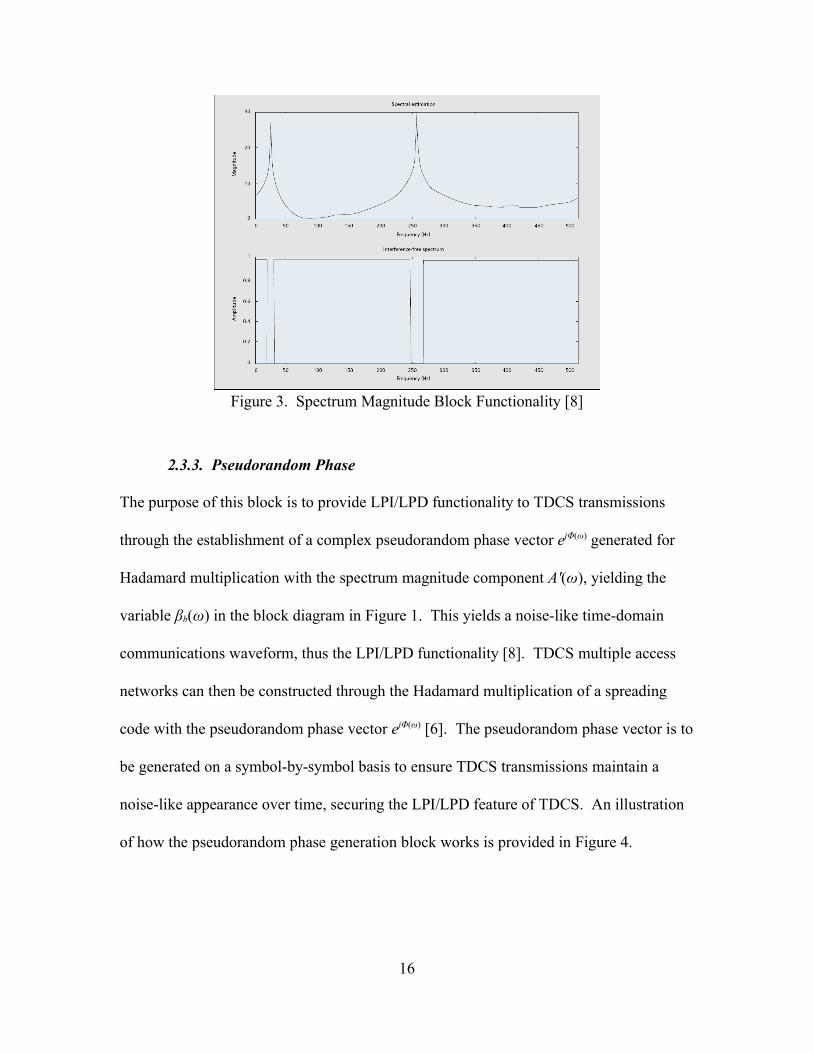
Figure 3. Spectrum Magnitude Block Functionality [8]
2.3.3. Pseudorandom Phase
The purpose of this block is to provide LPI/LPD functionality to TDCS transmissions
through the establishment of a complex pseudorandom phase vector ejΦ(ω) generated for
Hadamard multiplication with the spectrum magnitude component A'(ω), yielding the
variable βb(ω) in the block diagram in Figure 1. This yields a noise-like time-domain
communications waveform, thus the LPI/LPD functionality [8]. TDCS multiple access
networks can then be constructed through the Hadamard multiplication of a spreading
code with the pseudorandom phase vector ejΦ(ω) [6]. The pseudorandom phase vector is to
be generated on a symbol-by-symbol basis to ensure TDCS transmissions maintain a
noise-like appearance over time, securing the LPI/LPD feature of TDCS. An illustration
of how the pseudorandom phase generation block works is provided in Figure 4.
16

Figure 4. Pseudorandom Phase Vector Generation [8]
2.3.4. Scaling
Scaling of the complex frequency-domain signal βb(ω) is performed, yielding the
scaled signal β(ω). This ensures an appropriate amount of energy is contained in the
communications symbol to be transmitted, and that all communications symbols contain
the same amount of energy [8]. Thus, an appropriate bit error rate through the
communications channel is achieved, given the mapping between Eb/N0 and bit error rate
Pb.
2.3.5. IDFT
The spectrally encoded frequency-domain communications symbol β(ω) is inverse
Fourier transformed, yielding the time-domain symbol b(t) [8]. A waveform is generated
for each data symbol, so if two bits per symbol are to be transmitted, four symbols must
be constructed, thus four waveforms are generated. In the case of QPSK, the frequency-
domain waveform β(ω) is rotated using Hadamard multiplication with an additional
modulating vector to generate symbols that are 90, 180, or 270 degrees away from each
other. This is done through the use of a Hadamard multiplication with ejπ/2 for the second
17

symbol, ejπ for the third symbol , and ej3π/2 for the fourth symbol (neglecting Gray coding
in this description). These time-domain symbols will appear noise-like, thus increasing
the potential for LPI/LPD, through the multiplication with the pseudorandom phase
vector; and will intrinsically avoid interference, through the use of the spectral notching
algorithm.
A hardware implementation problem that has been observed in the use of any
modulation scheme that relies on an inverse Fourier transform (such as multicarrier
modulation) to generate time-domain communications waveforms is the construction of
symbols that contain exceptionally high peak-to-average power ratios (PAPR). Symbols
that contain high PAPR will exhibit instantaneous spikes of very large power, due to the
constructive addition in phase of subcarriers [16]. These spikes saturate the transmitter
power amplifier, force a clipping of the communications symbol, and cause
intermodulation distortion. This clipping inadvertently reduces the symbol energy and
creates a difference in symbol shape between the received time-domain symbol and the
demodulator matched filter reference symbol. Both of these problems increase the end-
to-end bit error rate. Several techniques have emerged to mitigate this phenomenon, such
as the use of the central limit theorem to limit the bounds of the envelope of the time-
domain communications symbol waveform [17].
2.3.6. Buffer
The purpose of this block is simply to provide a storage space for the
communications symbols (four symbols in the case of QPSK) for subsequent mapping
between data bits and symbol waveforms [8]. The refresh rate for the waveforms, the rate
18

at which spectrum estimation and spectral encoding occurs, depends on the requirements
of the communications system, and the channel variance over time.
2.3.7. Modulation/Transmission
Time-domain communications symbol waveforms are concatenated in accordance
with the mapping between data bits and symbol waveforms to generate a discrete-valued
time-domain communications signal. This signal is then converted to an analog signal
and radiated through the channel.
2.3.8. Receiver Architecture at Large
The TDCS receiver block diagram is illustrated in Figure 5. It contains blocks
used to locally generate time-domain reference signals cj(T), indicated by the dashed line
in the figure [8]. These reference signals are used in time-domain matched filter
correlation with received symbol waveforms to generate a test statistic zj(t) that is
compared with a maximum likelihood decision rule, yielding estimates of the symbol
most likely to have been received. The reference symbol associated with the output test
statistic with the highest magnitude becomes the symbol estimate, and is mapped to bits.
This is the same matched filter detection technique used in conventional correlation
receivers. The difference in receivers between those that use TD-PSK and those that use
conventional PSK is the process by which reference signals are generated. As can be
seen in Figure 5, five highlighted blocks are integrated to construct local symbol
waveforms. These blocks are used in the same manner as blocks of the same name in the
transmitter. This will yield identical transmitted signals and demodulator reference
signals, assuming both the transmitter and receiver are obtaining identical channel
19

Figure 5. TDCS Receiver Block Diagram [8]
spectrum estimates and that the pseudorandom phase vector is synchronized between the
transmitter and receiver. This creates a problem in implementing TDCS in hardware, as
the transmitter and receiver may not be obtaining identical spectrum estimates. The
results of simulations and experiments demonstrating the effect of spectrum estimate
mismatch are provided in Sections 4.3 and 5.4, respectively.
2.4. Synchronization of Received TDCS Signals
As stated in Section 2.1, Roberts performed the initial study into TDCS
synchronization, and concluded that DTC can be used to provide both peak and threshold
detection, which in turn yields synchronization and acquisition, respectively [3]. In order
to perform DTC, a predetermined synchronization codeword that is shared between the
transmitter and the receiver is translated into a preamble waveform [3]. This codeword
consists of a predetermined group of symbols that, when used in conjunction with a
buffer in the receiver, are used in both threshold and peak detection [3]. In threshold
detection, which provides signal acquisition, received signals and noise are continuously
20
zj(t) M
Estimatespectrum
IDFT
Spectrummagnitude
Scaling
Conj
cj(t)
Dashed line encloses FMW generation process(identical to process used by transmitter)
M
M( )
Tdt•∫
Decision rule
d(t)Data
r(t)
Pseudorandomphase

correlated with the predetermined codeword waveform [3]. The result of this correlation,
a simple dot product of the received signal and the predetermined codeword waveform,
will either be above or below a predetermined threshold. If the result of this dot product
is greater than the value of the threshold, than a decision is made within the receiver
programming that a TDCS signal is present. If no signal is determined to be present at
the receiver, no further processing is conducted by the receiver, beyond the ongoing
correlation for signal acquisition. However, if a signal is determined to be present, then
peak detection is performed, which yields symbol synchronization [3]. In peak detection,
correlation is performed again with the buffered received signal and the predetermined
codeword waveform. Correlation for peak detection again yields a simple dot product.
The difference in peak detection, however, is that the position in time of the peak value of
the correlation, rather than the amplitude of the correlation values, is important. The
position (in discrete samples) where the peak value of the correlation occurs should be the
position of the last sample of the synchronization waveform codeword. This sample,
along with all buffered samples before this sample, is discarded, as the position of the
start of the data waveform has been identified to be the next sample. Once this process is
complete, synchronization between the transmission and the receiver has been achieved.
2.5. Spectrally Modulated, Spectrally Encoded Signaling
Roberts recently published a digital communications framework for categorizing
modulation schemes that rely on SMSE signaling [11]. Roberts defines communications
signaling as SMSE when “both 1) data modulation [spectral modulation] and 2) encoding
[spectral encoding] are applied as amplitude and/or phase variations on a discrete
21

[frequency domain] component-by-component basis...” [11: 70]. The SMSE (or SMSE
signaling) framework integrates digital communications schemes that rely on waveform
design in the frequency domain into a mathematical framework for a cognitive radio-
based software defined radio. Examples of SMSE signaling include TDCS, multicarrier
code division multiple access (MC-CDMA), or one of the variants of orthogonal
frequency division multiplexing. The SMSE framework leverages modern vector and
matrix mathematics to functionally describe and design multicarrier- or subcarrier-based
communications symbols (for example, in MC-CDMA or TDCS, respectively). The
framework consolidates six waveform design variables to enable analytic unification for
SMSE signaling. These six variables, described as vectors by lower-case bold letters,
include the code c, the data modulation d, the window w, the orthogonality term o, the
assigned frequencies a, and the used frequencies u [11].
The code vector c is described as follows [11]:
1 2 1[ , ,..., ] [ ] , FF
NN i i ic c c c c== = ∈c £ (6)
where ci represents the value, which is complex numbered as denoted by £ , of the code
vector for the ith of the NF frequency subcarriers used in generating communications
symbols. In the case of TDCS signaling, the code vector consists of the series of
pseudorandom phase variations [11], as described in Section 2.3.3.
The data modulation vector d is described as follows [11]:
1 2 1[ , ,..., ] [ ] , FF
NN i i id d d d d== = ∈d £ (7)
where di represents the value, again which can be complex valued, of the data modulation
vector for the ith subcarrier. In the case of TD-QPSK, the data modulation vector d for
22
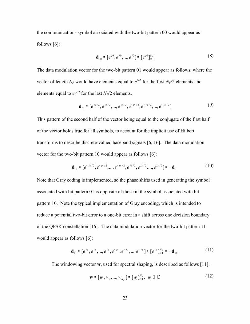
the communications symbol associated with the two-bit pattern 00 would appear as
follows [6]:
0 0 0 000 1[ , ,..., ] [ ] FNj j j j
ie e e e == =d (8)
The data modulation vector for the two-bit pattern 01 would appear as follows, where the
vector of length NF would have elements equal to ejπ/2 for the first NF/2 elements and
elements equal to e-jπ/2 for the last NF/2 elements.
/ 2 / 2 / 2 / 2 / 2 / 201 [ , ,..., , , ,..., ]j j j j j je e e e e eπ π π π π π− − −=d (9)
This pattern of the second half of the vector being equal to the conjugate of the first half
of the vector holds true for all symbols, to account for the implicit use of Hilbert
transforms to describe discrete-valued baseband signals [6, 16]. The data modulation
vector for the two-bit pattern 10 would appear as follows [6]:
/ 2 / 2 / 2 / 2 / 2 / 210 01[ , ,..., , , ,..., ]j j j j j je e e e e eπ π π π π π− − −= = −d d (10)
Note that Gray coding is implemented, so the phase shifts used in generating the symbol
associated with bit pattern 01 is opposite of those in the symbol associated with bit
pattern 10. Note the typical implementation of Gray encoding, which is intended to
reduce a potential two-bit error to a one-bit error in a shift across one decision boundary
of the QPSK constellation [16]. The data modulation vector for the two-bit pattern 11
would appear as follows [6]:
11 1 00[ , ,..., , , ,..., ] [ ] FNj j j j j j jie e e e e e eπ π π π π π π− − −
== = = −d d (11)
The windowing vector w, used for spectral shaping, is described as follows [11]:
1 2 1[ , ,..., ] [ ] , FF
NN i i iw w w w w== = ∈w £ (12)
23

where wi represents the value, again which can be complex numbered, of the windowing
vector for the ith subcarrier. In the case of TDCS signaling, the windowing vector
consists simply of all elements equal to one, or rectangular windowing [11].
The orthogonality vector o, which is used to induce orthogonality between
simultaneously transmitted signals in multiple access applications, is described as follows
[11]:
1 2 1[ , ,..., ] [ ] , , 1FF
NN i i i io o o o o o i== = ∈ = ∀o £ (13)
where oi represents the value, again which can be complex valued, of the orthogonality
vector for the ith subcarrier. For this design vector, each of the individual elements of the
vector has unit magnitude, as this vector is only used to rotate the phase of individual
frequency-domain subcarriers. In the case of a single user pair, there is no need to use an
orthogonality vector, so the elements of the vector are simply equal to one.
The frequency assignment vector a, dictated to individual user pairs by a multi-
user network controller to individual user pairs (enabling frequency division multiple
access) is described as follows [11]:
1 2 1[ , ,..., ] [ ] , {0,1}FF
NN i i ia a a a a== = ∈a (14)
where ai, valued at either 0 or 1, determines whether a potential frequency subcarrier is
allowed by the network controller for use by a user pair. In other words, if a set of
frequency subcarriers have frequency assignment vector elements equal to 1, then the
bands used by the associated frequency subcarriers are allowed for use by the user pair. If
an element associated with a subcarrier is equal to zero, then the frequency subcarrier is
24

not allowed for use by the user pair. In the scenario where only a single user pair is
involved, the elements of the frequency assignment vector are all equal to one.
The frequency use vector u is determined through a consensus within one user
pair to perform functions such as interference avoidance and coexistence (rather than
multiple access) assurance. The vector u is described as follows [11]:
1 2 1[ , ,..., ] [ ] , {0,1}FF
NN i i iu u u u u== = ∈u (15)
where ui equals 0 or 1 and dictates whether a potential frequency subcarrier is to be used.
As with the frequency assignment vector, if a set of subcarriers have frequency use vector
elements equal to 1, then the band used by the associated frequency subcarrier will
contain energy upon signal transmission. It is worth noting that, practically speaking, the
elements of the frequency use vector u will be equal to or smaller than the elements of the
frequency assignment vector a. Expressing this mathematically [11],
i iu a i≤ ∀ (16)
In all scenarios where CR-based SDR concepts are applied in a hardware implementation,
the frequency assignment vector will vary over time to compensate for environmental
conditions, to include the presence of interference in the channel. Discussion of specific
examples of the TDCS frequency use vector will be reserved for Section 3.1.2.
These six symbol design variables are consolidated to express the baseband value
of the kth symbol sk[m] as a series of NF terms through the following equation [11]:
( ), ,
1
,0
[ ]F
d c w om k m m m k
Nj
k m m m m k mm
s m a u c d w eθ θ θ θ
−+ + +
=
= (17)
25

where m is the index of the frequency component (the index of the subcarrier) and am, um,
cm, θc, dm,k, θd, wm, θw, and θo are the magnitudes (denoted by a letter) and phases (denoted
by θ) of the six design variables. Using row vector notation in the case of one user pair,
or matrix notation in the case of multiple user pairs (where each user pair occupies one
row of the matrix), the following equation expresses the time-domain output of (17),
sSMSE(t) [11]:
sSMSE t=F−1{ S k=A⊙θ⊙F } (18)
where Sk represents one of K distinct communications symbols that have been
concatenated together to form a signal for transmission. The variable A represents the
resulting magnitude vector of the Hadamard products of design variable magnitudes cm,
dm,k, wm; the variable Θ represents the resulting phase vector of the additions of design
variables θc, θd, θw, and θo; and the variable F, the frequency component identification
vector, represents the product of the Hadamard multiplication of the frequency
assignment and use vectors a and u. While this expression completely describes the
time-domain value of an SMSE-based communications symbol, it does not convey that
only the real value of a generated signal is radiated by an antenna, thus (18) is restated for
practical use as follows:
sSMSE t=ℜ{ F−1 {S k=A⊙θ⊙F }} (19)
While all symbol concatenation is performed in the time-domain in the TDCS
hardware implementation, Roberts asserts an additional variable for concatenating
symbols in the frequency domain, which exploits the relationship between delays in time
and phase shifts in frequency. All transmission waveforms can then be designed in the
26

frequency domain, so the final frequency-domain signal can be inverse Fourier
transformed to the time domain for transmission [11]. This approach may reduce latency
due to signal processing time requirements.
In the SMSE framework, a received signal rs[n] is expressed as [11]:
r [ ] s [ ]*h [ ] [ ]s s sn n n nη= + (20)
where hs[n] is the impulse response of the channel at time index n, * indicates a
convolution operator, and η[n] is the summation of all noise and interference. (20) is
simply the standard model for an end-to-end communications channel consisting of a
single user pair. Roberts goes further to expand this channel model by incorporating an
RF filter (be it a lowpass or bandpass filter) on the front end of the receiver for noise
reduction. This expansion of (20) for a single user pair that includes an RF filter is as
follows [11]:
( )r [ ] s [ ]*h [ ] [ ] h [ ]k s s rfn n n n nη= + ∗ (21)
where hrf[n] is the impulse response of the RF filter. As discussed in Section 2.9, the
practical design requirement for an RF filter is satisfied within the design of the DSK-
based hardware realization. An FFT is then performed on received signal rk[n] for
spectral demodulation [11]. As discussed in Section 3.5, the TDCS receiver design does
not use an FFT for processing received signals. Roberts modifies the TDCS receiver
design in his research for the purposes of describing TDCS within the SMSE framework
[11].
27
2.6. Equalization of Received TDCS Signals
Though DTC provides a means by which symbol waveforms can be synchronized,
DTC does nothing to mitigate phase offsets in the received signal caused by sample
timing offsets between the transmitter and receiver nor phase shifts induced by
propagation delays. Furthermore, the channel between the transmitter and receiver may
be less than ideal, consisting only of an impulse at time t = 0 (thus the impulse has no
delay). In a noiseless ideal channel, the received signal exactly equals the transmitted
signal [18]. A less than ideal channel, which is expected when constructing a hardware
implementation of a digital communications user pair, is one where a transmitted signal
incurs a phase delay and a channel consisting of multiple taps. Channel taps can result
from communicating in a multipath-laden environment [19]. As stated in Section 2.1,
Gaona studied TDCS performance in the presence of multipath propagated signals,
including the implementation of a RAKE receiver [7]. Using a RAKE receiver to
coherently reconstruct TDCS signals may be practical for a fixed-site user pair (such as
would be found in communications between buildings), but clearly isn't practical in
mobile communications. The prevalent method for mitigating the effects of a less-than-
ideal communications channels is through equalization [19]. Typical solutions for
equalizing received signals, in either a deterministic or a statistical manner, are a zero-
forcing or an MMSE equalizer, respectively [19]. Because an MMSE equalizer does
more to mitigate the effects of noise than a zero-forcing equalizer [19], an MMSE
equalizer has been implemented in hardware to address the issues of imperfect channels
and phase offsets in the received signal.
28

The mathematics in implementing an MMSE equalizer consist of several
computations based on matrix algebra. Given a received vector of distorted samples x of
finite length which composes the Toeplitz matrix X; a reference vector of undistorted
samples z[n] of finite length, referred to as a training sequence; and a channel response
vector c of finite length, with individual elements representing channel taps; the
following equation expresses how the channel response is computed for use in
equalization [19]:
1xx xz−=c R R (22)
Rxx, the autocorrelation matrix of the received samples, is calculated as follows [19]:
Hxx =R X X (23)
Rxz, the cross-correlation vector, is calculated as follows [19]:
Hxz =R X z (24)
The Toeplitz matrix X is generated for use in (23) and (24) by placing the values of the
received vector x in X in the following format [19]:
[ ] 0 0 0 0[ 1] [ ] 0
[ ] [ 1] [ 2] [1 ] [ ]
0 0 0 [ ] [ 1]0 0 0 0 [ ]
x Nx N x N
x N x N x N x N x N
x N x Nx N
− − + − = − − − −
−
X
LL L L
M M ML
M M MLL
(25)
The index of the received samples n = -N,...,N, the first column of (25), consists of a
vector where the first 2N+1 elements is the entire received vector x. The Toeplitz matrix
X is of size mxn, where m is two times the length of z minus one, and n is the length of z.
29
When used practically, z is modified with zero padding both before and after the training
values. If z is originally of length 19, z is modified with zero padding so that it is of
length 37. Zero padding is done with an equal number of elements before and after the
training values, so there would be nine elements of zero value both before and after
training values.
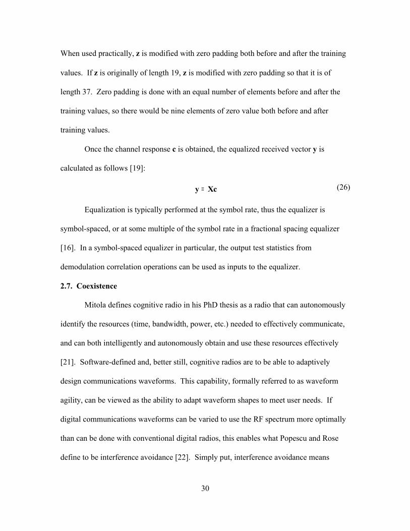
Once the channel response c is obtained, the equalized received vector y is
calculated as follows [19]:
=y Xc (26)
Equalization is typically performed at the symbol rate, thus the equalizer is
symbol-spaced, or at some multiple of the symbol rate in a fractional spacing equalizer
[16]. In a symbol-spaced equalizer in particular, the output test statistics from
demodulation correlation operations can be used as inputs to the equalizer.
2.7. Coexistence
Mitola defines cognitive radio in his PhD thesis as a radio that can autonomously
identify the resources (time, bandwidth, power, etc.) needed to effectively communicate,
and can both intelligently and autonomously obtain and use these resources effectively
[21]. Software-defined and, better still, cognitive radios are to be able to adaptively
design communications waveforms. This capability, formally referred to as waveform
agility, can be viewed as the ability to adapt waveform shapes to meet user needs. If
digital communications waveforms can be varied to use the RF spectrum more optimally
than can be done with conventional digital radios, this enables what Popescu and Rose
define to be interference avoidance [22]. Simply put, interference avoidance means
30

transmitting the most signal energy in areas where there is the least interference [22]. It is
further suggested here that this definition of interference avoidance holds true spectrally,
spatially, temporally, and among other areas of communications dimensionality. This
statement is inferred by Popescu and Rose as well [22].
User capacity C (bits per second) using the Shannon-Hartley capacity theorem, is
computed as follows, where W is the communications bandwidth (Hertz), S is the average
communications signal power (Watts), and N is the average noise power (Watts) [19]:
2log 1 SC WN
= + (27)
The mapping between SNR and Eb/N0 for baseband signals in an AWGN channel
is as follows [19], where Rb is the bit rate (bits/second):
0
b bE RSN N W
= (28)
Given (27) and (28), the capacity equation can be rewritten as follows:
20
log 1 b bE RC WN W
= +
(29)
Bit error rate Pb for a coherently detected M-ary PSK system, given Eb/N0 with
Gray coded symbol assignment, is expressed as follows [19], where M is the number of
communications symbol waveforms required to transmit a given number of bits per
symbol:
2
2 0
2 log ( )2 sinlog ( )
bb
M EP Q
M N Mπ ≈
(30)
31

Given (29) and (30) specifically for coherently detected M-ary PSK, the theoretic
transmission rate for a given channel and bit error performance can be associated as
follows:
2
1 22
2
log ( )1 1log 12log ( ) 2sin
b b
UNCODED
M P RC W QM W
Mπ
−
= +
(31)
This association allows for the assertion of a codependent relationship between bit
error rate, SNR, bandwidth, and the required transmission rate. This codependence
defines one of the fundamental tradeoffs in communications engineering: how best to
manage resources to transmit information at a given bit error rate. While admittedly this
relationship does not take forward error correction coding into consideration,
acknowledgment of this codependent relationship allows the first of the two requirements
for cognitive radio to be addressed. This assertion furthermore means coexistence
between independently functioning communications resource users (users not operating
in a multiple access network) can be addressed in a framework shared by all users of the
communications resource. Acknowledgment and management of this codependency
enables cognitive communication, as defined by Mitola [21], for all users of the
communications medium.
Another way of looking at channel capacity theory is by taking this view of the
problem: a given channel will permit a fixed number of information bits per second to be
communicated through the channel. This fixed number is divided among all users of the
channel. If all users are operating using the same SNR, the same bit rate, the same
32
forward error correction scheme, the same modulation type, and the same bandwidth and
center frequency, capacity theory can be used to determine the maximum number of users
operating at a given signal-to-interference plus noise-ratio (SINR) [22]. High data rate
modulation types simply take up a larger share of the total channel capacity available to
all users. Through being able to avoid interference and by properly identifying the
resources required to communicate, cognition is reached. By managing (29) and (31), a
multi-user view of communications cognition can be taken. If one can accurately
estimate the PSD of a channel over time, manage the codependent communications
variables which compose (31), and communicate using agile waveforms to best
accommodate a time-varying channel, one truly achieves communications cognition.
The ability to coexist in a manner that more optimally uses communications
resources requires that all users of a given spectrum perform interference avoidance to
deconflict their transmissions with each other, thus coexist. This is not how a multiple
access network behaves, where users of the network operate given a set of predetermined
rules; coexistence means there are no rules. This gives way to what is called greedy
interference avoidance, where each user greedily maximizes its own SINR given a user
pair's ability to provide feedback on interference conditions from the receiver to the
transmitter [22]. What Popescu and Rose assert is the counterintuitive conclusion that the
use of greedy interference avoidance tends to optimize the use of communications
resources (in terms of sum capacity) [22]. What Popescu, Popescu, and Rose have found
is that optimization of sum capacity is usually reached through what is called water-filling
in general information theory. The use of water-filling means that each user is operating
33
in its own self-interest to maximize SINR [23]. This gives way to what Clemens and
Rose have implicitly identified as the fundamental precept of spectrum management in
unlicensed, thus laissez faire, bands: cognitive radio (awareness of the environment and
the ability to adapt to the environment) will be required to achieve optimal coexistence
[24].
2.8. Coexistence and the Pursuit of LPI/LPD Communications
For an LPI/LPD communications system to be effective at avoiding detection, the
system must be able to coexist with other communicators. The premise is that if a
coexistent user of the spectrum of interest is suffering from degraded performance when
the system of interest is transmitting, but doesn't suffer from degraded performance when
the system of interest is not transmitting, the coexistent user becomes aware that
something is using the spectrum. The coexistent user, whether the other user even knows
it or not, is detecting the system of interest. This means the system of interest should not
be classified as LPD, leading to the conclusion that coexistence is a non-negotiable
requirement in an LPD communications system. Therefore, coexistence enables not only
interference avoidance, but LPI/LPD capability as well.
Initial TDCS research involved the explicit use of different kinds of jamming
signals to simulate interference. This definition can be broadened without any
breakdowns in the simulations and mathematics simply by asserting that jammers are, if
present in the spectrum, in and of themselves simply the most aggressive interferers. In
this context, the goal of TDCS is simply to coexist undetected.
34
2.8.1. Water-filling
Water-filling in the context of communications resource management is explained
by Cover and Thomas as follows:
The vertical levels indicate the noise levels in the various channels. As signal power is increased from zero, we allot the power to the channels with the lowest noise. When the available power is increased still further, some of the power is put into noisier channels. The process by which the power is distributed among the various bins is identical to the way in which water distributes itself in a vessel [25: 253].
This explanation is explicitly stated here because Cover and Thomas are cited when
defining water-filling in [22] and [23]. Cover and Thomas provide a definition of water-
filling that enables adaptive communications symbol waveform design in a manner that,
in the words of Popescu and Rose, yields optimal use of the RF spectrum [22]. Popescu
and Rose apply Cover and Thomas provide an equation to define water-filling, but for the
purposes of this research, water-filling is taken as a concept, rather than a specific
equation, so no specific mathematical equation is used.
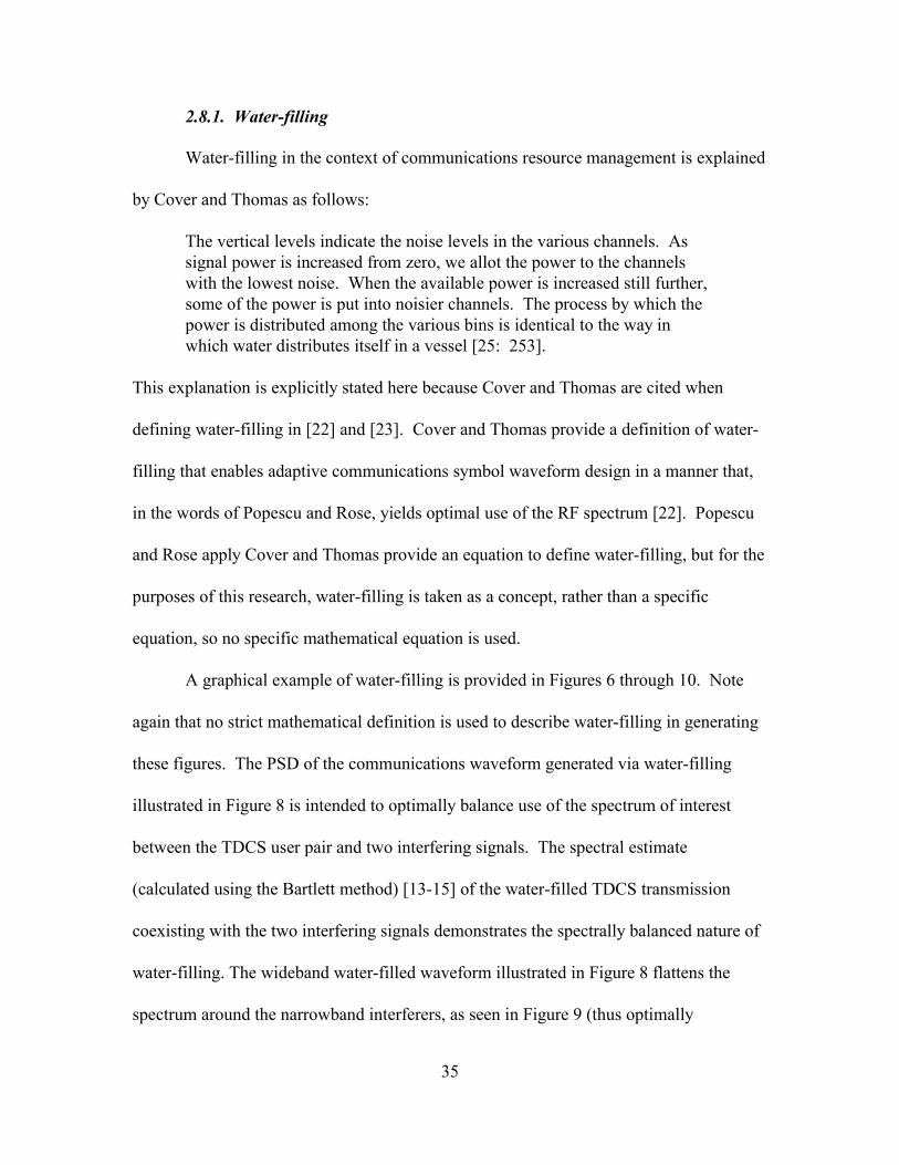
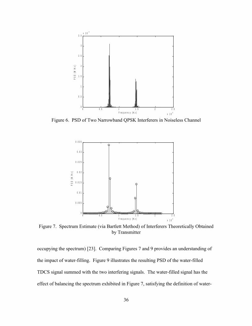
A graphical example of water-filling is provided in Figures 6 through 10. Note
again that no strict mathematical definition is used to describe water-filling in generating
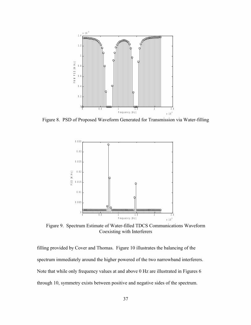
these figures. The PSD of the communications waveform generated via water-filling
illustrated in Figure 8 is intended to optimally balance use of the spectrum of interest
between the TDCS user pair and two interfering signals. The spectral estimate
(calculated using the Bartlett method) [13-15] of the water-filled TDCS transmission
coexisting with the two interfering signals demonstrates the spectrally balanced nature of
water-filling. The wideband water-filled waveform illustrated in Figure 8 flattens the
spectrum around the narrowband interferers, as seen in Figure 9 (thus optimally
35
0 0 . 5 1 1 . 5 2 2 . 5
x 1 04
0
0 . 5
1
1 . 5
2
2 . 5
3
3 . 5x 1 0
- 4
F r e q u e n c y ( H z )
PS
D (
W/H
z)
Figure 6. PSD of Two Narrowband QPSK Interferers in Noiseless Channel
0 0 . 5 1 1 . 5 2 2 . 5
x 1 04
0
0 . 0 0 5
0 . 0 1
0 . 0 1 5
0 . 0 2
0 . 0 2 5
0 . 0 3
0 . 0 3 5
F r e q u e n c y ( H z )
PS
D (
W/H
z)
Figure 7. Spectrum Estimate (via Bartlett Method) of Interferers Theoretically Obtained by Transmitter
occupying the spectrum) [23]. Comparing Figures 7 and 9 provides an understanding of
the impact of water-filling. Figure 9 illustrates the resulting PSD of the water-filled
TDCS signal summed with the two interfering signals. The water-filled signal has the
effect of balancing the spectrum exhibited in Figure 7, satisfying the definition of water-
36
0 0 . 5 1 1 . 5 2 2 . 5
x 1 04
0
0 . 2
0 . 4
0 . 6
0 . 8
1
1 . 2
1 . 4x 1 0
- 3
F r e q u e n c y ( H z )
FM
W P
SD
(W
/Hz)
Figure 8. PSD of Proposed Waveform Generated for Transmission via Water-filling
0 0 . 5 1 1 . 5 2 2 . 5
x 1 04
0
0 . 0 0 5
0 . 0 1
0 . 0 1 5
0 . 0 2
0 . 0 2 5
0 . 0 3
0 . 0 3 5
F r e q u e n c y ( H z )
PS
D (
W/H
z)
Figure 9. Spectrum Estimate of Water-filled TDCS Communications Waveform Coexisting with Interferers
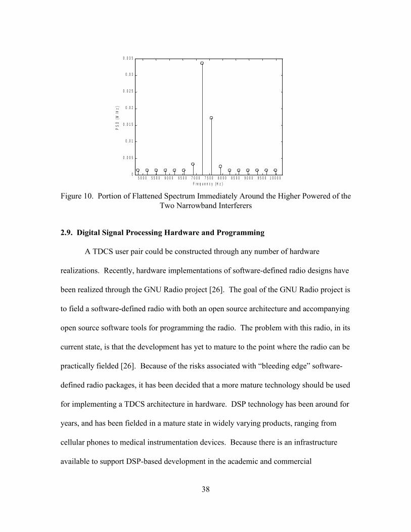
filling provided by Cover and Thomas. Figure 10 illustrates the balancing of the
spectrum immediately around the higher powered of the two narrowband interferers.
Note that while only frequency values at and above 0 Hz are illustrated in Figures 6
through 10, symmetry exists between positive and negative sides of the spectrum.
37
5 0 0 0 5 5 0 0 6 0 0 0 6 5 0 0 7 0 0 0 7 5 0 0 8 0 0 0 8 5 0 0 9 0 0 0 9 5 0 0 1 0 0 0 00
0 . 0 0 5
0 . 0 1
0 . 0 1 5
0 . 0 2
0 . 0 2 5
0 . 0 3
0 . 0 3 5
F r e q u e n c y ( H z )
PS
D (
W/H
z)
Figure 10. Portion of Flattened Spectrum Immediately Around the Higher Powered of the Two Narrowband Interferers
2.9. Digital Signal Processing Hardware and Programming
A TDCS user pair could be constructed through any number of hardware
realizations. Recently, hardware implementations of software-defined radio designs have
been realized through the GNU Radio project [26]. The goal of the GNU Radio project is
to field a software-defined radio with both an open source architecture and accompanying
open source software tools for programming the radio. The problem with this radio, in its
current state, is that the development has yet to mature to the point where the radio can be
practically fielded [26]. Because of the risks associated with “bleeding edge” software-
defined radio packages, it has been decided that a more mature technology should be used
for implementing a TDCS architecture in hardware. DSP technology has been around for
years, and has been fielded in a mature state in widely varying products, ranging from
cellular phones to medical instrumentation devices. Because there is an infrastructure
available to support DSP-based development in the academic and commercial
38

communities, it is believed that a DSP-based implementation is less risky than a more
novel hardware technology.
There are several different technical challenges in implementing a digital
communications system onboard a hardware platform. Interfacing the AIC23
Coder/Decoder (codec), which contains the analog-to-digital converter (ADC) and the
digital-to-analog converter (DAC), with the DSP chip onboard the DSK requires
particular attention. In order to obtain input samples of the noisy, interference-laden
spectrum and/or the communications signal of interest, the ADC onboard the codec is
used [27]. The ADC converts an analog acoustic signal into a digital value. This digital
value is then transferred to the DSP chip for processing. The processed outputs to be
emitted from the DSP chip are passed back to the codec where they are converted from
digital values to analog signal levels through use of the DAC.
When sampling received signals at a rate of 48 kHz using the AIC23 codec, an
anti-aliasing filter is automatically applied to the received signal [28]. This anti-aliasing
filter serves as the RF filter described in (21).
39

III. TDCS Architecture Implementation
Implementing a TDCS, as with any other engineering effort, requires the designer
to make choices based on informed trade-offs. The approach taken in this research effort
is to integrate theory with pragmatic solutions to existing problems. A few areas where
trade-offs and design choices are made in this research include:
● Choosing a technique for use in spectrum estimation.
● Designing communications symbol waveforms in the presence of an
indeterminate, suboptimal (less than flat) end-to-end spectrum response.
● Managing the need to equalize the received TDCS signal.
This chapter outlines these design choices made in implementing TDCS in hardware, and
integrates the notation offered by Roberts' proposed framework for SMSE digital
communications [11] discussed in Section 2.5 into the TDCS architecture.
3.1. Transmitter
Figure 1 illustrates the general TDCS transmitter block diagram commonly
published in literature [8]. The SMSE framework discussed in Section 2.5 has brought
about the need to revise the block diagram to incorporate the notation used in the SMSE
framework. Figure 11 illustrates the updated TDCS transmitter block diagram used in the
implementation of the DSK-based design.
3.1.1. Spectrum Estimation
Spectrum estimation is performed using the Bartlett method, as discussed in
Section 2.3.1. The absolute magnitude of the spectrum estimate at a given frequency is
not required, as the spectrum estimate is only used to perform communications symbol
40

f[m ]
Φ[m ]
c[m ]
s[n]sk[n]s
k[n]
s(t)Estimatespectrum
Pseudorandomphase
IDFT Buffer Modulation(bits-to-symbols)
Transmission
Data (bitstream)
Spectrummagnitude
sk[m] s
k[m ]
ScalingData (waveform)modulation
dk[m]
Figure 11. TDCS Transmitter Block Diagram Incorporating SMSE Notation
waveform design. This being the case, spectrum estimation is performed by calculating
the periodograms of subsequences of samples of the noisy environment. The
periodograms are then summed, which yields a relative PSD estimate between various
frequencies in the environment. This estimate can then be used to perform waveform
design.
Performing accurate spectrum estimation in a hardware implementation that uses
a wireless channel is complicated by hardware limitations. While the DSK is capable of a
sampling frequency of 48 kHz, with a frequency response that is assumed to be flat
throughout the codec passband, the microphone used to sample the acoustic environment
may have a much smaller bandwidth than the DSK. The microphone may also have a
less than optimal magnitude response within its passband, though no attempt is made in
this research to characterize the frequency response of the microphone. In an interference
avoiding digital communications design, spectrum estimation of a noisy environment is
performed to identify frequency bands that have been compromised by the presence of
41

interference. If the hardware involved in this process is integrated together in such a
manner that the end-to-end signal path between the noisy environment and the digital
processor is suboptimal, then areas of the spectrum where the magnitude response of the
estimation hardware is relatively high will seemingly exhibit more noise than areas where
the magnitude response is relatively low. This phenomenon will drive the uninformed
user of the interference avoidant system to avoid areas of the spectrum where the
magnitude response of the hardware is highest, as the user operates under the impression
that these frequencies are compromised. If the transmitter and receiver use the same
hardware for reception of interference avoidant signals as for spectrum estimation, parts
of the spectrum that may be most favorable for transmission of signals go ignored in
favor of less suitable frequency bands. On the other hand, the interference avoidant
waveforms generated through spectrum magnitude calculations will load power in areas
of the spectrum where the estimation hardware may have no magnitude response at all.
In this case, if the transmitter and receiver use the same hardware for reception of
interference avoidant signals as for spectrum estimation, then signal power will be
transmitted in areas of the spectrum that may go entirely unreceived. More power may
then be wasted through the use of interference avoidance algorithms than would be
through conventional waveform design techniques. No interference avoidant
communications design is free from this difficulty. As discussed in Section 2.7, Mitola
describes cognitive radio as the ability to intelligently and autonomously use
communications resources effectively [21]. Therefore, if a hardware implementation of a
software-defined radio architecture does not perform estimation of the end-to-end
42
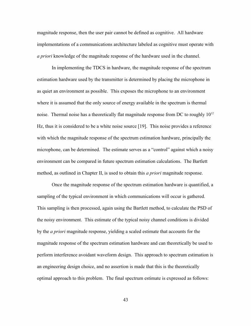
magnitude response, then the user pair cannot be defined as cognitive. All hardware
implementations of a communications architecture labeled as cognitive must operate with
a priori knowledge of the magnitude response of the hardware used in the channel.
In implementing the TDCS in hardware, the magnitude response of the spectrum
estimation hardware used by the transmitter is determined by placing the microphone in
as quiet an environment as possible. This exposes the microphone to an environment
where it is assumed that the only source of energy available in the spectrum is thermal
noise. Thermal noise has a theoretically flat magnitude response from DC to roughly 1012
Hz, thus it is considered to be a white noise source [19]. This noise provides a reference
with which the magnitude response of the spectrum estimation hardware, principally the
microphone, can be determined. The estimate serves as a “control” against which a noisy
environment can be compared in future spectrum estimation calculations. The Bartlett
method, as outlined in Chapter II, is used to obtain this a priori magnitude response.
Once the magnitude response of the spectrum estimation hardware is quantified, a
sampling of the typical environment in which communications will occur is gathered.
This sampling is then processed, again using the Bartlett method, to calculate the PSD of
the noisy environment. This estimate of the typical noisy channel conditions is divided
by the a priori magnitude response, yielding a scaled estimate that accounts for the
magnitude response of the spectrum estimation hardware and can theoretically be used to
perform interference avoidant waveform design. This approach to spectrum estimation is
an engineering design choice, and no assertion is made that this is the theoretically
optimal approach to this problem. The final spectrum estimate is expressed as follows:
43

1
0
ˆ [ ][̂ ] ˆ [ ]
FN
Noisy
White m
mm
mφ
φφ
−
=
=
(32)
where m represents the index of a given frequency domain “subcarrier” and NF represents
the number of frequency-domain subcarriers in the communications symbol waveform.
The output of the spectrum estimation algorithm for a single realization of noise
plus interference, expressed in terms of the variables in (32), is illustrated in Figure 12.
This realization is generated using the Matlab® wavplay and wavrecord functions with
PC speakers and microphone. A single tone interferer is present in the noisy spectrum at
a frequency of 2.000 kHz. This interference appears as it should in the figure, with
interference present in the noisy and final estimates at and around 2 kHz. While only
frequency values at and above 0 Hz are illustrated in Figure 12, symmetry exists between
positive and negative sides of the spectrum.
3.1.2. Spectrum Magnitude Calculation
As stated in Section 2.3.2, the spectrum magnitude output consists simply of a
vector of ones and zeros, as implied in Figure 3 [8]. This vector serves as the frequency
component identification vector f[m] in the SMSE framework, as described in Section
2.5, and is the Hadamard product of the frequency assignment vector a and the frequency
use vector u, so
{ } 1
0[ ] [ ] [ ] FN
mm m m −
==f a u (33)
As stated in Section 2.5, the frequency assignment vector is dictated to users by a network
controller, so the frequency assignment vector is disregarded. The frequency use vector,
on the other hand, provides the means by which the TDCS interference avoidance
44
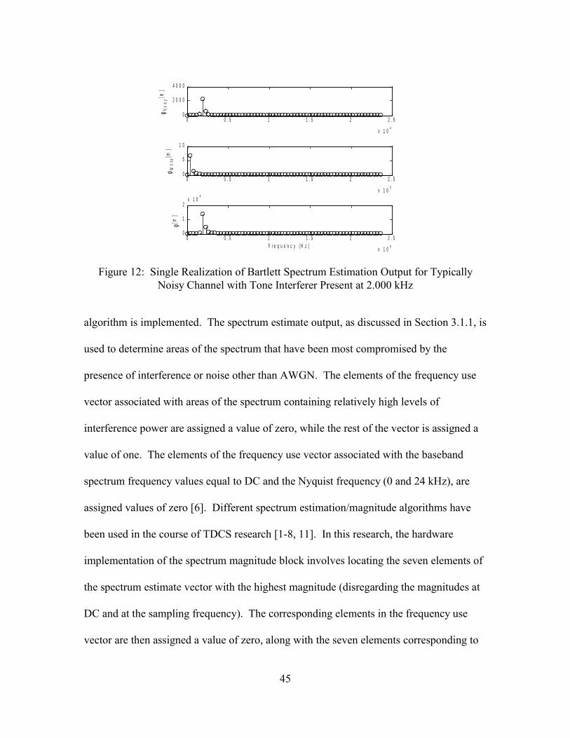
0 0 . 5 1 1 . 5 2 2 . 5
x 1 04
0
2 0 0 0
4 0 0 0
φ Noi
sy[m
]
0 0 . 5 1 1 . 5 2 2 . 5
x 1 04
0
5
1 0
φ Whi
te[m
]
0 0 . 5 1 1 . 5 2 2 . 5
x 1 04
0
1
2x 1 0
4
φ[m]
F r e q u e n c y ( H z )
Figure 12: Single Realization of Bartlett Spectrum Estimation Output for Typically Noisy Channel with Tone Interferer Present at 2.000 kHz
algorithm is implemented. The spectrum estimate output, as discussed in Section 3.1.1, is
used to determine areas of the spectrum that have been most compromised by the
presence of interference or noise other than AWGN. The elements of the frequency use
vector associated with areas of the spectrum containing relatively high levels of
interference power are assigned a value of zero, while the rest of the vector is assigned a
value of one. The elements of the frequency use vector associated with the baseband
spectrum frequency values equal to DC and the Nyquist frequency (0 and 24 kHz), are
assigned values of zero [6]. Different spectrum estimation/magnitude algorithms have
been used in the course of TDCS research [1-8, 11]. In this research, the hardware
implementation of the spectrum magnitude block involves locating the seven elements of
the spectrum estimate vector with the highest magnitude (disregarding the magnitudes at
DC and at the sampling frequency). The corresponding elements in the frequency use
vector are then assigned a value of zero, along with the seven elements corresponding to
45
the same frequency on the opposite side of the spectrum. There are several reasons this
approach to spectral notching has been taken. First, it allows for an interference
algorithm to be incorporated into the design without having to perform scaling on a
symbol-by-symbol basis, as described in Section 2.3.4. Second, this approach is
relatively simple to implement. Third, there is little processing latency associated with
this approach. Fourth, this approach ensures the same number of subcarriers are “notched
out” on both the transmit and receive sides of the user pair. Finally, since there is no
means by which spectral notching information is being communicated from transmitter to
receiver (which would most likely require error correction coding, and is outside the
scope of this thesis), spectrum estimation and spectrum frequency use vector mismatches
will occur in hardware experiments. This will lead to suboptimal symbol estimation and
an increase in bit error curves. Given this is the case, initiating interference avoidance for
a small subset of the available subcarriers allows for interference avoidance
experimentation on a limited scope without compromising the results as a whole. An
illustration of the output vector of the spectrum magnitude operation is provided in Figure
13. This figure is generated using the same scenario used to generate the illustration of
the spectrum estimation process provided in Figure 12. Note that 14 subcarriers, plus the
frequencies associated with DC and the Nyquist frequency, are “zeroed out” in the
frequency assignment vector f[m]. The decision to notch out 14 subcarriers (disregarding
the subcarriers at DC and the Nyquist frequency) incidentally brings this research effort in
line with Roberts' work in SMSE signaling. In the bit error performance curves generated
through simulations that involve spectral notching, Roberts used partial band interference
46

0 0 . 5 1 1 . 5 2 2 . 5
x 1 04
0
5 0 0 0
1 0 0 0 0
1 5 0 0 0
φ[m]
0 0 . 5 1 1 . 5 2 2 . 5
x 1 04
0
0 . 5
1f[
m]
F r e q u e n c y ( H z )
Figure 13: Single Realization of Spectrum Magnitude Output for Typically Noisy Channel with Tone Interferer Present at 2.000 kHz
that spanned 10% of the available frequencies [11]. If spectral notching is used with 128
total subcarriers, notching out 14 of these subcarriers reduces the available spectrum by
10.9%. The 14 subcarrier frequencies where the most interference is observed, plus the
subcarriers at DC and the Nyquist frequency, will be notched out. While only frequency
values at and above 0 Hz are illustrated in Figure 13, symmetry exists between positive
and negative sides of the spectrum.
3.1.3. Pseudorandom Phase Generation
As stated in Sections 2.3.3 and 2.5, the pseudorandom phase generation operation
consists of establishing a uniformly distributed and complex-valued pseudorandom code
vector c[m] to spectrally encode communications symbol waveforms. The magnitude of
the elements of the complex-valued code vector are all of unit magnitude [1-8, 11], and
are Hadamard multiplied with the frequency assignment vector f[m] discussed in Section
3.1.2. Though the TDCS transmitter block diagram in Figure 11 does nothing to express
47

this, the orthogonality vector o[m] described in Section 2.5 can be Hadamard multiplied
with the code vector to produce communications symbols that are suitable for multiple
access applications.
In practice, the code vector is generated by randomly assigning phase angles of
positions on the unit circle to elements within the code vector. The phase angles are
equally spaced on the unit circle, thus a uniform distribution is achieved. While the code
vector is to be generated on a transmitted symbol-by-symbol basis to ensure LPI/LPD
functionality is maintained, it is assumed that all code vectors exhibit equivalent bit error
performance. It is further assumed that all communications symbols are mutually
independent from one another in terms of demodulation (and subsequent bit error
performance), so only one realization of a code vector is used in the hardware
implementation. This is done to ease the computational burden in the hardware
realization. As with (8)-(11), the code vector is actually split in half to account for the
implicit use of Hilbert transforms to describe discrete-valued baseband signals [6, 18].
Therefore, the first half of the baseband spectrum is assigned negative phase angles
between 0 and 2π radians, while the second half of the baseband spectrum is assigned a
reflection of the first half around the y-axis. The reflection in the second half is then
multiplied by -1 to account for the implicit use of Hilbert transforms. The elements of the
code vector associated with the DC and Nyquist frequencies are always assigned values
of zero, and held out of the pseudorandom phase vector generation process. The values
of the code vector at DC and Nyquist frequency element positions is irrelevant, since the
frequency assignment vector has values of zero at these two elements, so no power will
48

be present at these two frequencies during symbol transmission. One realization of a
generated code vector is illustrated in Figure 14. The value of Θ[m] illustrates the nature
of the reflection around the y-axis.
3.1.4. Data (Waveform) Modulation
Data modulation is conducted using the data modulation vectors d00[m], d01[m],
d10[m], and d11[m] expressed in (8)-(11) respectively. In a TD-QPSK design, four distinct
communications symbols are required. These four data modulation vectors answer this
requirement. The data modulation vectors are Hadamard multiplied with the frequency
assignment vector and the code vector. The resulting symbol waveform, sk[m], is
expressed as follows:
{ } 1
0[ ] [ ] [ ] [ ] FN
k k mm m m m −
==s f c d (34)
where k denotes the symbol index.
The reason TD-QPSK is used exclusively in the hardware implementation is to
provide a means by which orthogonal, rather than simply antipodal, signaling can be
studied. Section 2.5 describes how the data modulation vectors used for this research are
constructed.
3.1.5. Scaling
As stated in Section 2.3.4, scaling is performed on the complex-valued frequency domain
communications symbol waveforms s00[m], s01[m], s10[m], and s11[m] to ensure that a
required bit error performance is obtained regardless of the number of elements that are
valued at one or zero in the frequency identification vector f[m]. If the number of
frequency subcarriers activated for use with the frequency identification vector varies,
49
- 2 . 5 - 2 - 1 . 5 - 1 - 0 . 5 0 0 . 5 1 1 . 5 2 2 . 5
x 1 04
- 1 0
0
1 0
θ[m]
P s e u d o r a n d o m p h a s e
- 2 . 5 - 2 - 1 . 5 - 1 - 0 . 5 0 0 . 5 1 1 . 5 2 2 . 5
x 1 04
- 1
0
1
Rea
l(c[m
])
- 2 . 5 - 2 - 1 . 5 - 1 - 0 . 5 0 0 . 5 1 1 . 5 2 2 . 5
x 1 04
- 1
0
1
Imag
inar
y(c[
m])
F r e q u e n c y ( H z )
Figure 14. Single Realization of Pseudorandom Code Vector c[m] for Use in Spectral Encoding
scaling is performed to maintain the bit energy level required to sustain a given error rate.
Given that a fixed number of elements in the frequency identification vector are set to
zero in the hardware implementation, there is no need to account for this function in the
hardware implementation.
3.1.6. IDFT
As stated in Section 2.3.5, the complex-valued frequency domain communications
symbols s00[m], s01[m], s10[m], and s11[m] are inverse Fourier transformed, yielding time
domain symbols s00[n], s01[n], s10[n], and s11[n], respectively. An FFT function is
provided by Chassaing [27] for use onboard the DSK. This “black box” FFT function
can be used to perform an IFFT by simply adding a 1/N scaling factor (where N is the
number of complex-valued points in the FFT computations) and conjugating the twiddle
factors used in the FFT algorithm [27].
50

Section 2.3.5 discusses a potential problem in hardware implementation of
multicarrier modulation schemes where constructed time-domain waveforms may exhibit
exceptionally high PAPR. This problem is intrinsically addressed, as scaling is
performed on the time-domain symbols to raise or lower the peak instantaneous
magnitude of all four symbols to the maximum possible magnitude output by the DSK
codec. This error-free scaling is enabled through the use of floating-point arithmetic in
either the Matlab®-based TDCS implementation or the DSK-based implementation,
and is performed using the same scale factor for all four time-domain communications
symbol waveforms used in TD-QPSK. The communications symbol sk[n] after scaling is
expressed as
( ) ( ) ( ) ( )( )128 128 128 12800 01 10 111 1 1 1
[ ][ ]max max [ ] , max [ ] , max [ ] , max [ ]
kk
k k k k
nn Gn n n n
= = = =
← sss s s s
(35)
where G is the maximum magnitude the DSK codec is capable of outputting, thus the
peak value of the TDCS signal transmission will be equal to G.
Generated communications symbols, representing one realization of TD-QPSK
time-domain communications waveforms, are illustrated in Figure 15, assuming a
maximum signal output magnitude G equal to one. The four communications symbols
illustrated in Figure 15 are concatenated together in a time-domain waveform, in
accordance with the mapping of bits to symbols dictated by the data bitstream input to the
TDCS transmitter. The noise-like structure of the waveforms, is due to the spectrally
encoded nature of the waveforms, and works to enable LPI/LPD. Note also that between
the symbols s00[n] versus s11[n] and s01[n] versus s10[n] that the symbols opposite in bit
51

0 0 . 5 1 1 . 5 2 2 . 5 3
x 1 0- 3
- 1
0
1
s 00[n
]
I D F T
0 0 . 5 1 1 . 5 2 2 . 5 3
x 1 0- 3
- 1
0
1
s 01[n
]
0 0 . 5 1 1 . 5 2 2 . 5 3
x 1 0- 3
- 1
0
1s 10
[n]
0 0 . 5 1 1 . 5 2 2 . 5 3
x 1 0- 3
- 1
0
1
s 11[n
]
T i m e ( s e c )
Figure 15. Time-domain Communications Signal Waveforms for TD-QPSK Signaling
pattern (00 versus 11 and 01 versus 10) are the opposite symbol reflected around the x-
axis. In other words, s00[n] equals -s11[n] and s01[n] equals -s10[n], as is expected with
QPSK signaling. Finally, symbols s00[n] and s11[n] are both orthogonal to symbols s01[n]
and s10[n], as is expected in TD-QPSK signaling [6]. It is appropriate to point out that the
symbol waveforms are illustrated using a “connect-the-dots” plot rather than a stem plot.
This is done only to cleanly communicate the appearance of the waveform.
3.1.7. Buffer
As stated in Section 2.3.6, the buffer is used to provide a storage for the
communications symbols. The DSK-based hardware implementation has buffer space
intrinsically built within the design. In the design of the hardware user pair, there is no
refreshing of the symbols stored in the buffer within the one-second transmission burst. It
is assumed that the spectrum estimate will not vary enough to merit a refreshing.
52

3.1.8. Modulation (Bits-to-Symbols)/Transmission
As stated in Section 2.3.7, modulation refers to the mapping of bit patterns to
communications symbols. Two-bit patterns contained in input bitstreams are mapped to
communications waveforms that are concatenated in time in preparation for transmission.
An illustration of the constellation used in this TD-QPSK design is provided in Figure 16.
Note that Gray coding is used in mapping bit patterns to communications symbols.
As stated in Section 2.3.7, transmission consists of converting the final digital
TDCS signal data vector s[n] to analog signal s(t) and the subsequent transmission of the
analog signal into the channel.
3.2. Acquisition of Received Signals
Acquisition of TDCS signals is performed by manually directing the transmitting
DSK and the receiving DSK to operate simultaneously. This process is initiated by
simultaneously toggling dip switches on the transmitting and received boards. The
receiving DSK stores the one-second burst output to the channel by the transmitting DSK
into a buffer sized to store a two-second recording from the receiver microphone.
3.3. Synchronization of Received Signals
Synchronization of TDCS signals is performed using peak detection, as discussed
in Section 2.4, and is conducted using only the DTC method. The minimum Eb/N0 value
required to evaluate the bit error performance is 0 dB, the TDCS hardware realization
operates at a baseband two-sided bandwidth of 48.000 kHz, and 128 samples/symbol are
arbitrarily used. Given these conditions, the lowest SNR used in hardware experiments is
approximately -18 dB, per (28). Roberts determined that for an 80% probability of
53
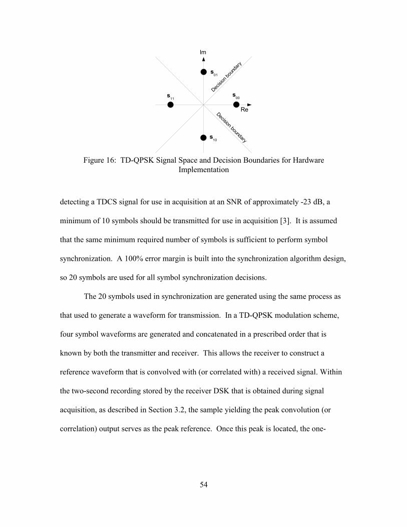
Re
Im
s00
s01
s10
s11
Decision boundary
Decisio
n bou
ndary
Figure 16: TD-QPSK Signal Space and Decision Boundaries for Hardware Implementation
detecting a TDCS signal for use in acquisition at an SNR of approximately -23 dB, a
minimum of 10 symbols should be transmitted for use in acquisition [3]. It is assumed
that the same minimum required number of symbols is sufficient to perform symbol
synchronization. A 100% error margin is built into the synchronization algorithm design,
so 20 symbols are used for all symbol synchronization decisions.
The 20 symbols used in synchronization are generated using the same process as
that used to generate a waveform for transmission. In a TD-QPSK modulation scheme,
four symbol waveforms are generated and concatenated in a prescribed order that is
known by both the transmitter and receiver. This allows the receiver to construct a
reference waveform that is convolved with (or correlated with) a received signal. Within
the two-second recording stored by the receiver DSK that is obtained during signal
acquisition, as described in Section 3.2, the sample yielding the peak convolution (or
correlation) output serves as the peak reference. Once this peak is located, the one-
54

second TDCS transmission burst (as well as noise, interference, and channel effects due
to such phenomena as multipath propagation) is identified.
3.4. Reception and Demodulation of Received Signals
Figure 5 illustrates the general TDCS receiver block diagram published in the
literature. As with the TDCS transmitter, the SMSE framework discussed in Section 2.5
has brought about the need to revise the block diagram to incorporate the notation used in
the SMSE framework. Figure 17 illustrates the updated receiver block diagram used in
the implementation of the DSK-based design.
The receiver block diagram in Figure 17 includes several common functions with
the transmitter diagram illustrated in Figure 11, including “Estimate spectrum,”
“Spectrum magnitude,” “Data (waveform) modulation,” “Pseudorandom phase,” and
“IDFT.” This highlights the fact that the transmitter and receiver perform the same
operations to construct communications symbol waveforms on both the transmit-side and
receive-side of the user pair. The only difference is that only two waveforms are required
for demodulation (though all the waveforms are generated by the receiver to construct a
reference signal for use in synchronization). These two waveforms, expressed in the
block diagram as s00[n] and s01[n], serve as inphase and quadrature reference signals when
performing TD-QPSK demodulation. Subscripts 00 and 01 are used to convey that the
waveform mapped to the two-bit symbol 00 is used in correlation to generate the X
statistic, while the waveform mapped to the two-bit symbol 01 is used to generate the Y
statistic. The lines with arrows through the reference waveforms s00[n] and s01[n] convey
that these waveforms are generated adaptively through the spectrum magnitude function
55

Figure 17. TDCS Receiver Block Diagram Incorporating SMSE Notation
shared by both the transmitter and receiver. Once these reference waveforms are
generated, a synchronized received signal is demodulated using these waveforms. The
output values from the correlation, X and Y, are input to a four-quadrant arctangent
operation. The output of this operation serves to assign a phase value to the received
symbol in question. This phase value is compared with a decision rule used to determine
a final symbol estimate, si. The specific decision rule being used in the implemented
demodulator, as stated in Section 3.1.8, is illustrated in Figure 16. An illustration of a
received and demodulated TD-QPSK symbol constellation is provided in Figure 18. The
constellation for Eb/N0 = 9.85 dB uses the decision boundaries illustrated in Figure 16.
Each data point in Figure 18 represents the test statistic output value from a single
communications symbol, so there are 375 data points illustrated in Figure 18. Note that
the constellation points exhibit a phase offset around the unit circle and that there is some
degree of variance around the centroid of each of the clusters of points. This variance is
56
X =∑n=1
N
r [n]s00 [n]
f[m]
Φ[m]
c[m]
sk[n]
Estimatespectrum
Pseudorandomphase
IDFT
Spectrummagnitude
sk[m]
Data (waveform)modulation
dk[m]
r(t)s
00[n]
s01
[n]
Estimatespectrum
tan-1(Y/X) Decisionrule
Y=∑n=1
N
r [n]s01[n]
si

- 0 . 1 5 - 0 . 1 - 0 . 0 5 0 0 . 0 5 0 . 1 0 . 1 5
- 0 . 1 5
- 0 . 1
- 0 . 0 5
0
0 . 0 5
0 . 1
0 . 1 5
I n p h a s e
Qua
drat
ure
B e f o r e e q u a l i z a t i o n , Eb
/ N0
= 9 . 8 5 d B , E r r o r s = 3 / 7 5 0
Figure 18. Demodulated TD-QPSK Symbol Constellation of 375 Demodulated Symbols at Eb/N0 = 9.85 dB Communicated in a Single One-Second Burst
due to noise, be it AWGN, intersymbol interference, and/or an interfering signal present
near the receiver. Demodulation of this specific realization of TDCS signaling yielded
three bit errors out of 750 total transmitted bits.
An RF filter, as described in (21), is incorporated intrinsically into the design of
the receiver when incorporating the TDCS algorithm onboard the DSK. This RF filter is
brought about through the use of the anti-aliasing filter built into the codec, and is
described in Section 2.9.
3.5. Equalizing Received Signals
As discussed in Section 2.6, the hardware realization includes an MMSE equalizer
that is implemented as described in (22)-(26). The MMSE equalizer requires a reference
signal for training, and is used in generating the cross-correlation vector Rxz. The
reference signal is obtained by performing a demodulation operation on the reference
waveform used for synchronization. The output test statistics from the correlators are
57

then placed into a complex-valued format. The first 19 of the 20 symbols used to
construct the synchronization reference waveforms are used in training the equalizer, thus
the equalizer is permitted 19 filter taps. Once correlation is performed on a received
TDCS signal and the test statistics output from the two correlators are available, the first
19 of the received symbol statistic outputs are placed into Toeplitz matrix X, as expressed
in (25). The autocorrelation matrix Rxx of the received symbol test statistics is then
calculated, as stated in (23). Computation of Rxx is performed by multiplying matrices
containing complex-valued elements, so a Hermetian transpose is used. The first 19, as
opposed to 20, symbols are used to generate z because an odd-numbered length is easier
to process. This allows the Toeplitz matrix X to be assembled using elements from x that
range from index -N to N, as opposed to having to zero-pad a leading or trailing element
in the x and/or z vector. In the hardware implementation, computing the autocorrelation
matrix, as with all matrix-matrix and matrix-vector multiplication operations, requires
either an extensive effort to manage the computation of complex valued matrices, or the
use of library functions. One such set of functions for performing complex arithmetic in
C-based programs is offered by Press, Flannery, Teukolsky, and Vetterling [29]. These
functions are integrated into the design of the software onboard the receive-side DSK.
Once the autocorrelation matrix is computed, it is multiplied with the cross-correlation
vector, as expressed in (22), to obtain the equalizer coefficients, which requires a matrix
inverse operation. Though literature is explicit in stating that direct matrix inverse
computation is to be avoided [30], the decision was made to perform matrix inverse
operations via the Gauss-Jordan method [20], thus the matrix is inverted directly. While
58

direct computation of matrix inverses are intensive, the inverse of a 19x19 matrix is not
unreasonably expensive. An algorithm performing direct inversion of a complex-valued
matrix is embedded into the equalizer design and requires less than one second to
compute onboard the DSK. This approach is not recommended for real-time operations,
however, and the positive semi-definite nature of the autocorrelation matrix lends itself to
a more efficient calculation of the inverse. Regardless, the entire vector of received
complex-valued symbol test statistics are input into a Toeplitz matrix, as seen in (25).
The Toeplitz matrix is multiplied by the vector of equalizer taps, yielding the equalized
channel test statistic estimates used to demodulate the signal. This set of estimates then
theoretically represents symbol test statistics in which noise, ISI, and phase offsets are
mitigated.
In the design of the hardware user pair, there is no retraining past the initial
training of the equalizer. This is because the TDCS signal is transmitted in a one-second
burst, and it is assumed that the channel response will not vary enough to merit a
refreshing of the equalizer training.
Figure 19 illustrates the effect that equalization can have on received symbol test
statistics. Figure 19 is generated using an equalized version of the same realization of
received symbol test statistic values as those used to generate Figure 18. As in Figure 18,
each data point in Figure 19 represents the test statistic output value from a single
communications symbol, so there are 375 data points illustrated in Figure 19. The three
received bit errors illustrated in Figure 18 are corrected through equalization. The
differences between Figures 18 and 19 are obvious, as the phase offset is corrected and
59

- 2 0 - 1 5 - 1 0 - 5 0 5 1 0 1 5 2 0- 2 0
- 1 5
- 1 0
- 5
0
5
1 0
1 5
2 0
I n p h a s e
Qua
drat
ure
A f t e r e q u a l i z a t i o n , Eb
/ N0
= 9 . 8 5 d B , E r r o r s = 0 / 7 1 2
Figure 19. Equalized TD-QPSK Symbol Constellation of 375 Demodulated Symbols at Eb/N0 = 9.85 dB in Same One Second Burst Used in Figure 18
the variances around the cluster centroids are reduced, relative to the scale of the decision
regions. Though this is only one example of equalization, the effectiveness of the MMSE
equalizer is visually obvious.
3.6. Computing SNR and Eb/N0
As expressed in (28), there is a linear relationship between SNR and Eb/N0. The
bit error curves provided in Chapter V illustrate bit error rates relative to Eb/N0, but in
reality, SNR is computed at the receiver and then Eb/N0 is subsequently calculated using
(28). SNR is simply the average power PS of the received TDCS signal r[n] divided by
the average power PN of the noise received simultaneously with the signal. Noise power
can be closely approximated by the following relationship [19]:
2 2N N NP mσ≅ + (36)
where σN2 is the variance of noise samples and mN is the mean value of noise samples.
Note that (36) assumes that the noise is wide-sense stationary, so the noise has a constant
60
mean and an autocorrelation as a function of n1 – n2 alone [31]. The assumption is made
in the hardware implementation that all noise and interference has zero mean, and that
any realizations of received signals have a non-zero mean only because of a bias voltage
in the ADC. Given this assumption, the mean value of a received realization r[n] can
then be neglected. The transmitted signal s[n] has zero mean as a result of the uniformly
distributed phase encoding employed in the TDCS design. After synchronization of the
received signal, there are N = 48000 samples in the one second time window within
which the TDCS transmission resides. The value of each sample is simply the sum of the
received TDCS transmission r[n] at time index n plus the sum of all noise and
interference present in the received signal at time index n. Given the assumption that
noise plus interference has zero mean, the noise power PN can be estimated per (36)
simply by computing the variance of the noise plus interference. The following
expression is used to compute the sample variance of the noise plus interference [31], and
together with (36) yields an estimate of the power PN of all noise plus interference:
480002 2
1
1 ( [ ] [ ])47999N N
nP r n s nσ
=
≅ = −∑ (37)
The expression in (37) is normalized by N-1 rather than N samples (47999 versus 48000)
to perform unbiased estimation of the sample variance. Unbiased estimation of the
variance has been chosen because the noise plus interference signal available to the DSK
represents a sampling, rather than the population, of the signal. Note that (37) assumes
that the noise plus interference samples are independent and identically distributed.
The use of (37) is limited to instances when the magnitude of the received TDCS
signal s[n] is known. Given the received signal is the sum of the received TDCS signal
61
and all noise plus interference simultaneously present in the environment, the magnitude
of the received TDCS signal must be scaled to accurately calculate the noise power. This
scaling in turn intrinsically yields an estimate of received TDCS signal power. To
perform this estimate, the mean square error (MSE) criterion is used. The function used
to estimate the power PS of the received TDCS signal, using the MSE criterion, is as
follows [27]:
248000
01
minarg [ ] [ ]
[0, )Sn S
KP K r n s nK σ=
≅ = − ∈ ∞ ∑ (38)
where K represents a scale factor and σS is the standard deviation of s[n]. The value of K
that minimizes the argument, K0, is equal to PS, so all that is required to compute SNR is
the power of the sum of noise plus interference, PN. Given the scaled version of the
received TDCS signal, and the assumption that noise plus interference has zero mean, it
is assumed that the noise plus interference power can be computed as follows:
248000
0
1
1 [ ] [ ]47999N
n S
KP r n s n
σ=
= −
∑ (39)
Therefore, (28) can be restated as follows:
02
480000 0
1
1 [ ] [ ]47999
b
bn S
E WKN K
R r n s nσ=
=
− ∑
(40)
where W is the bandwidth (Hz) and Rb is the bit rate (bits/second). For practical purposes,
(40) accurately expresses how all Eb/N0 calculations are made in generating the results
provided in Chapter V.
62
IV. Spectral Notching Versus Water-filling
This chapter outlines research conducted to determine whether or not water-filling
is a more optimal means than spectral notching for generating TDCS communications
symbol waveforms. TDCS literature is explicit in stating that the spectral notching
algorithm described in Section 2.3.2 may not be optimal [3], and no attempt has been
made to optimize TDCS waveform designs. As discussed in Section 2.8.1, the optimal
means by which available spectrum is occupied is usually a water-filled solution [22, 23].
Though this statement has several conditions placed on it in literature, it suggests that a
water-filling waveform design algorithm may provide an advantage over spectral
notching. This suggestion motivates the simulations conducted in this chapter. If water-
filling indeed usually optimally uses the available spectrum, and if spectral notching
performs equivalently to water-filling in any given scenario, then spectral notching must
usually optimally use the available spectrum as well.
Formal Matlab® simulations are conducted to determine whether a water-filling
algorithm yields better bit error performance than spectral notching. This comparison is
reasonable, as both the water-filled and spectrally notched waveforms contain the same
amount of energy and occupy the same amount of bandwidth. The water-filling
algorithm is used directly in identifying which areas of the spectrum of interest are
notched out. The only difference between the water-filled and the spectrally notched
waveforms is how power is distributed in various areas of the spectrum. The implication
of using a water-filling algorithm, or any sort of frequency-domain waveform sculpting
63
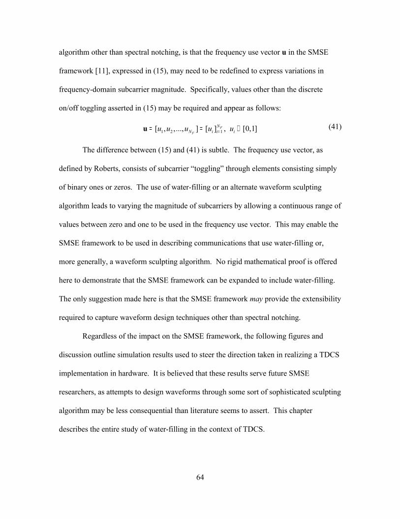
algorithm other than spectral notching, is that the frequency use vector u in the SMSE
framework [11], expressed in (15), may need to be redefined to express variations in
frequency-domain subcarrier magnitude. Specifically, values other than the discrete
on/off toggling asserted in (15) may be required and appear as follows:
1 2 1[ , ,..., ] [ ] , [0,1]FF
NN i i iu u u u u== = ∈u (41)
The difference between (15) and (41) is subtle. The frequency use vector, as
defined by Roberts, consists of subcarrier “toggling” through elements consisting simply
of binary ones or zeros. The use of water-filling or an alternate waveform sculpting
algorithm leads to varying the magnitude of subcarriers by allowing a continuous range of
values between zero and one to be used in the frequency use vector. This may enable the
SMSE framework to be used in describing communications that use water-filling or,
more generally, a waveform sculpting algorithm. No rigid mathematical proof is offered
here to demonstrate that the SMSE framework can be expanded to include water-filling.
The only suggestion made here is that the SMSE framework may provide the extensibility
required to capture waveform design techniques other than spectral notching.
Regardless of the impact on the SMSE framework, the following figures and
discussion outline simulation results used to steer the direction taken in realizing a TDCS
implementation in hardware. It is believed that these results serve future SMSE
researchers, as attempts to design waveforms through some sort of sophisticated sculpting
algorithm may be less consequential than literature seems to assert. This chapter
describes the entire study of water-filling in the context of TDCS.
64

All Eb/N0 computations are performed at the point of the simulated receiver
antenna. Unless explicitly stated, each data point in simulated bit error curves in Figures
20 to 22 are generated using at least 1000 bit errors.
4.1. TDCS Performance: Spectral Notching vs. Water-filling
The comparison of bit error performance of the TDCS user pair involves
simulating the transmission of TDCS waveforms through an AWGN channel containing
two randomly spread QPSK interferers and then processing the TDCS signals received
through the simulated channel. The interferers are spread using a randomly generated
CDMA spreading code. Demodulation is performed independently using the water-
filling and spectral notching algorithm. The TDCS user pair shares four communications
symbols used in a TD-QPSK modulation scheme. The interferers are implemented using
a bit energy equal to the bit energy of the TDCS transmission, so Eb/N0 will be equal for
all three users of the spectrum. The locations of the frequency components are the same
for both the spectrally notched and the water-filled TDCS communications symbols. The
water-filling algorithm is used to directly identify frequency subcarriers suitable for use in
spectral notching, so the TDCS transmission bandwidth is equal in both the spectral
notching and water-filling case. Figure 20 illustrates TDCS bit error performance using
spectral notching and water-filling over an interference-laden AWGN channel. The two
curves appear to be approximately equivalent; spectral notching and water-filling appear
to perform approximately equivalently in this scenario. Furthermore, both simulated
curves appear to be roughly equivalent to the analytic curve.
65
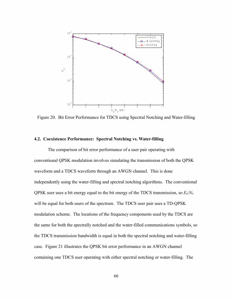
0 1 2 3 4 5 6 71 0
- 4
1 0- 3
1 0- 2
1 0- 1
E b / N o ( d B )
Pb
A n a l y t i c
W a t e r f i l l i n gN o t c h i n g
Figure 20. Bit Error Performance for TDCS using Spectral Notching and Water-filling
4.2. Coexistence Performance: Spectral Notching vs. Water-filling
The comparison of bit error performance of a user pair operating with
conventional QPSK modulation involves simulating the transmission of both the QPSK
waveform and a TDCS waveform through an AWGN channel. This is done
independently using the water-filling and spectral notching algorithms. The conventional
QPSK user uses a bit energy equal to the bit energy of the TDCS transmission, so Eb/N0
will be equal for both users of the spectrum. The TDCS user pair uses a TD-QPSK
modulation scheme. The locations of the frequency components used by the TDCS are
the same for both the spectrally notched and the water-filled communications symbols, so
the TDCS transmission bandwidth is equal in both the spectral notching and water-filling
case. Figure 21 illustrates the QPSK bit error performance in an AWGN channel
containing one TDCS user operating with either spectral notching or water-filling. The
66

0 1 2 3 4 5 6 71 0
- 4
1 0- 3
1 0- 2
1 0- 1
E b / N o ( d B )
Pb
A n a l y t i c
W a t e r f i l l i n gN o t c h i n g
Figure 21. Bit Error Performance for QPSK User Coexisting with TDCS User (No Interference Present)
two curves appear to be approximately equivalent. Given this is the case, spectral
notching and water-filling appear to coexist roughly equivalently with a typical digital
communications user pair. Furthermore, the QPSK user pair is performing roughly
equivalently with what would be expected given the analytic curve in an AWGN channel
with no interference. This being the case, TDCS user pairs appear to coexist with other
users, regardless of which waveform design algorithm is used.
4.3. Spectrum Estimate Mismatch: Spectral Notching vs. Water-filling
The comparison of bit error performance of the TDCS user pair involves
simulating the transmission of TDCS waveforms through an AWGN channel containing
two randomly spread QPSK interferers and then processing the TDCS signals received
through the simulated channel. The difference between this scenario and the original
study of TDCS bit error performance is that the spectrum estimates used by the TDCS
67

transmitter and receiver are no longer equal. Independent realizations of noise and
interference are generated for use independently by the TDCS transmitter and receiver,
though the pseudorandom phase vector is synchronized between transmitter and receiver.
This will have the effect of mismatching the TDCS signals received by the TDCS
receiver and the reference signals generated by the TDCS receiver for use in matched
filter detection. The test statistics output by the demodulator will then be less than
optimally computed. This simulation is performed using the water-filling and spectral
notching algorithms independently. The TDCS user pair uses a TD-QPSK modulation
scheme. The interferers are implemented using a bit energy equal to the bit energy of the
TDCS transmission, so Eb/N0 will be equal for all three users of the spectrum. The
locations of the frequency components used for transmission are the same for both the
spectrally notched and the water-filled TDCS communications symbols, so the TDCS
transmission bandwidth is equal in both the spectral notching and water-filling case.
Figure 22 illustrates the bit error performance of a TDCS user pair communicating in an
interference-laden AWGN channel when there is a mismatch between TDCS transmitter
and TDCS receiver spectrum estimates. Each point along the simulated curves is
generated using at least 2000 bit errors. Note that the two curves appear to be
approximately equivalent. There is a roughly equivalent degradation in performance in
both the spectral notching and water-filling cases, versus a scenario where the spectrum
estimates are equal between transmitter and receiver. The loss due to the spectrum
estimate mismatch is, in its worst case, almost 1.0 dB, at an Eb/N0 between 0 and 7 dB.
68

0 1 2 3 4 5 6 71 0
- 4
1 0- 3
1 0- 2
1 0- 1
E b / N o ( d B )
Pb
A n a l y t i c
W a t e r f i l l i n gN o t c h i n g
Figure 22. Bit Error Performance for Spectrally Mismatched TDCS User Pair
4.4. Interpretation of Simulation Results
In all three simulation scenarios in Sections 4.1 through 4.3, spectral notching and
water-filling yield roughly equivalent bit error performance in an AWGN channel. The
comparison of TDCS performance using both spectral notching and water-filling (Figure
20) and the comparison of a randomly spread QPSK user pair coexisting with a TDCS
transmission (Figure 21) demonstrate that, regardless of the waveform design algorithm, a
TDCS user pair coexists with interferers in the spectrum of interest.
The degradation in bit error performance seen in the case where spectrum
estimates are mismatched between TDCS transmitter and receiver is less than 1 dB in an
AWGN channel at an Eb/N0 between 0 and 7 dB.
4.5. Summary
Given the result that spectral notching and water-filling yield roughly equivalent
bit error performance, this implies that balancing the PSD of the TDCS signals through
69
water-filling may not be as important as literature implies [22]. However, one should not
infer that a water-filling approach has no value, as water-filling allows us to set a
threshold that intrinsically distributes power in the most appropriate manner for a given
Eb/N0. In an AWGN channel, the weighing function used to balance power among the
frequency components in the spectrum magnitude algorithm may not provide any
advantage over spectral notching. Spectral notching is much less computationally intense
than water-filling, so using a threshold to generate spectral notches may be the best
solution for a TDCS user. There may be a more optimal weighting scheme that can be
used to distribute symbol waveform power in the spectrum, but these results lend to a
degree of skepticism about this possibility. Water-filling is intended to optimize use of
the spectrum in terms of sum capacity, so as data rates are increased among coexistent
users of the spectrum, there may be motivation to use water-filling rather than spectral
notching.
The degradation in bit error performance in the scenario where the spectrum
estimates are mismatched between the TDCS transmitter and receiver is not as severe as
might be expected. This implies that, in an AWGN channel, synchronization between
transmitter and receiver spectrum estimates may not be critical in all instances to
communicate somewhat effectively. In this instance, whether this result has value to the
user depends entirely on what the user requires in terms of bit error performance.
70
V. Hardware Implementation Results
Four different scenarios are examined to address the research objective: to prove,
through successful TDCS signaling in a hardware implementation, that the concept of
TDCS-based digital communications is viable. For all four scenarios, the number of
received bit errors is computed both with and without use of the MMSE equalizer
discussed in Section 3.5. These scenarios are as follows:
1. No spectral notching with no narrowband interference added to the environment,
2. No spectral notching with narrowband interference added to the environment,
3. Spectral notching with narrowband interference added to the environment, and
4. Spectral notching with no narrowband interference added to the environment (to
examine the effects of potential spectral mismatch).
Figure 23 illustrates the equipment positioning used to generate all results
provided herein. There is a separation of approximately 0.30 meters between transmitter
speakers and receiver microphone in all experiments. The transmitter speaker volume is
adjusted to control the gain of the transmitted signal. The narrowband interfering signal
consists of a sinusoidal tone generated via Matlab® and transmitted using PC speakers.
The narrowband tone resides at randomly chosen frequencies between 1.500 and 22.500
kHz, and remains at a constant frequency and magnitude throughout the duration of a
one-second (750 bits/second) TDCS transmission.
Figures 24 through 31 illustrate the bit error performance observed in each of the
four different scenarios. There are 100 empirically obtained points in each of the eight
figures. In the cases where an equalizer is not used (Figures 24, 26, 28, and 30), 750
71

Figure 23. Photograph Illustrating Equipment Positioning During All DSK-based Experiments
received bits are compared with true values to determine bit error performance. In the
cases where an equalizer is used (Figures 25, 27, 29, and 31), 712 received bits are
compared with true values to determine bit error performance (750 bits are transmitted
and received, with 38 of these bits communicated in the 19 training symbols in the
preamble to the message). In all instances, the bit error rate is plotted against the received
Eb/N0 calculated as described in Section 3.6. Each of the figures includes the analytic
curve for M-ary PSK signaling expressed by (30) for comparison, where M = 4
communications symbols required to transmit 2 bits per symbol. In each of the
observations, colored noise may be present, so differences between empirically obtained
observations and the analytic curve may not be absolute. The curve is intended to serve
as a reference point for the observations at large, both within and between figures.
Although narrowband interference and other interference sources are colored, Eb/N0 is
used in all figures (versus SNR or SINR) to enable comparison with TD-QPSK
72

performance curves found in literature, particularly those developed by Nunez [6].
Semilogarithmic plots are not provided, as is typically the case in a bit error performance
plot. This is because many empirical observations yielded zero bit errors, which cannot
be accurately illustrated in a semilogarithmic plot.
All comparisons are made qualitatively, rather than quantitatively. This is
because SNR is deliberately uncontrolled in these experiments, to test the utility of the
spectral notching algorithm and the use of the MMSE equalizer in the TDCS architecture.
Because of the undefined and dynamic nature of the frequency magnitude and phase
responses of the speakers and microphones, it is believed that there is no way to
practically construct controlled experiments without the use of more sophisticated
hardware and test environments (such as an acoustic chamber). As will be seen, these
figures provide results that can be used for qualitative comparison.
5.1. No Spectral Notching with No Interference Added to Environment
Figure 24 illustrates the unequalized bit error performance of the hardware
realization when no spectral notching is applied and when there is no deliberately
generated interference present in the environment. Figure 25 illustrates the equalized bit
error performance using the same realizations of received TDCS signals as those used in
generating Figure 24.
The trend of the empirical bit error performance illustrated in Figure 24 appears to
coincide with the analytic curve. The trend of the empirical bit error performance
illustrated in Figure 25, on the other hand, indicates that bit error performance is
improved by the equalizer at an Eb/N0 above approximately -15 dB. The equalizer
73

- 1 0 0 - 8 0 - 6 0 - 4 0 - 2 0 0 2 00
0 . 1
0 . 2
0 . 3
0 . 4
0 . 5
0 . 6
0 . 7
Eb
/ N0
( d B )
Pb
N o n o t c h i n g , n o i n t e r f e r e n c e , u n e q u a l i z e d
A n a l y t i c
E m p i r i c a l
Figure 24. Unequalized Bit Error Performance Curve of Hardware Realization. No Spectral Notching in an Environment Without Additional Narrowband Interference
- 1 0 0 - 8 0 - 6 0 - 4 0 - 2 0 0 2 00
0 . 1
0 . 2
0 . 3
0 . 4
0 . 5
0 . 6
0 . 7
Eb
/ N0
( d B )
Pb
N o n o t c h i n g , n o i n t e r f e r e n c e , e q u a l i z e d
A n a l y t i c
E m p i r i c a l
Figure 25. Equalized Bit Error Performance Curve of Hardware Realization. No Spectral Notching in an Environment Without Additional Narrowband Interference
actually appears to degrade bit error performance below -15 dB. While this could be
interpreted to mean that the equalizer should not be used when the received Eb/N0 is
below -15 dB, the bit accuracy rate at this low SNR already approaches the coin flip
74

probability of 0.5, so it is not believed that TD-QPSK would be practically attempted
under these circumstances. The reason for the performance improvement on the part of
the equalizer, to the point where the performance exceeds the analytical curve, is because
the MMSE equalizer mitigates some noise effects by design [19]. Judging from Figures
24 and 25 together, it is believed that the hardware realization is performing as it should,
and that the firmware used to control the transmitter and receiver is correctly written.
5.2. No Spectral Notching with Interference Added to Environment
Figure 26 illustrates the unequalized bit error performance of the hardware
realization when no spectral notching is applied and when there is deliberately generated
narrowband interference present in the environment. Figure 27 illustrates the equalized
bit error performance using the same realizations of received TDCS signals as those used
in generating Figure 26.
The trend of the empirical bit error performance illustrated in Figure 26 appears to
coincide with the analytic curve. The trend of the empirical bit error performance
illustrated in Figure 27, on the other hand, indicates that bit error performance is
improved by the equalizer above approximately -15 dB, while the equalizer degrades bit
error performance below -15 dB. This is the case in Scenario 1 as well. When comparing
Figures 25 and 27, the presence of deliberately applied narrowband interference in the
spectrum of interest appears to only minimally impact the performance of the TDCS user
pair operating with the MMSE equalizer when no spectral notching is used.
75
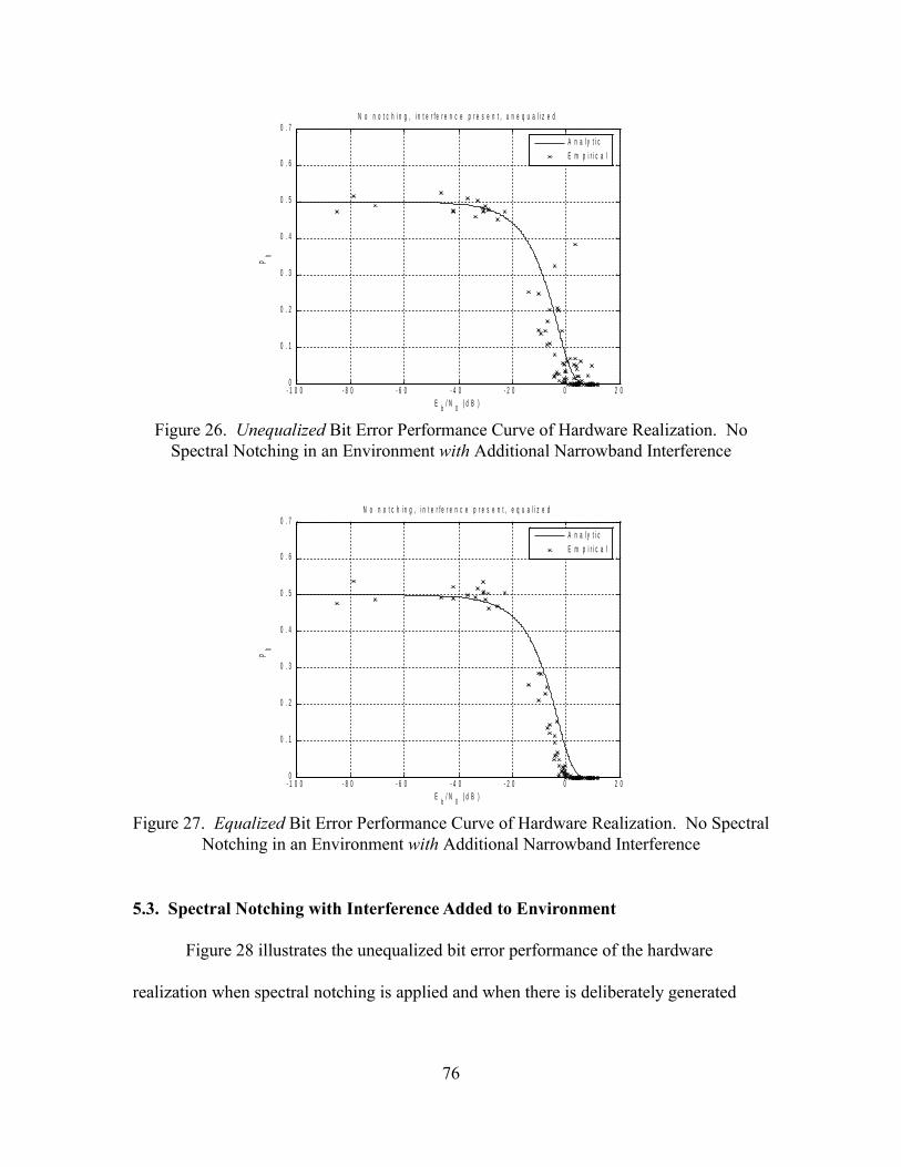
- 1 0 0 - 8 0 - 6 0 - 4 0 - 2 0 0 2 00
0 . 1
0 . 2
0 . 3
0 . 4
0 . 5
0 . 6
0 . 7
Eb
/ N0
( d B )
Pb
N o n o t c h i n g , i n t e r f e r e n c e p r e s e n t , u n e q u a l i z e d
A n a l y t i c
E m p i r i c a l
Figure 26. Unequalized Bit Error Performance Curve of Hardware Realization. No Spectral Notching in an Environment with Additional Narrowband Interference
- 1 0 0 - 8 0 - 6 0 - 4 0 - 2 0 0 2 00
0 . 1
0 . 2
0 . 3
0 . 4
0 . 5
0 . 6
0 . 7
Eb
/ N0
( d B )
Pb
N o n o t c h i n g , i n t e r f e r e n c e p r e s e n t , e q u a l i z e d
A n a l y t i c
E m p i r i c a l
Figure 27. Equalized Bit Error Performance Curve of Hardware Realization. No Spectral Notching in an Environment with Additional Narrowband Interference
5.3. Spectral Notching with Interference Added to Environment
Figure 28 illustrates the unequalized bit error performance of the hardware
realization when spectral notching is applied and when there is deliberately generated
76

narrowband interference present in the environment. Figure 29 illustrates the equalized
bit error performance using the same realizations of received TDCS signals as those used
in generating Figure 28.
The empirical bit error performance illustrated in Figures 28 and 29 both appear
to be different from the performance illustrated in Figures 24 and 26 or Figures 25 and
27, respectively (when comparing the unequalized cases or the equalized cases). In both
Figures 28 and 29, bit error performance above approximately -35 dB appears to be
superior to the analytic curve. This is due to the fact that the Eb/N0 estimation algorithm
outlined in Section 3.6 simply separates the received signal into either the TDCS
transmission or noise plus interference, while the use of N0 implies that the PSD of the
noise is flat. When spectral notching is used, an interfering signal is avoided by the
TDCS user pair, thus that portion of the spectrum is avoided. The noise plus interference
content in that area of the spectrum should not be weighed as heavily as in parts of the
spectrum that are used by the TDCS user pair, in order to obtain true SINR measurements
or Eb/N0 calculations at the receiver. The Eb/N0 estimation algorithm, which yields Eb/N0
estimates observed at the position immediately after signals are output from the receive-
side microphone, does not weigh parts of the spectrum that are disregarded by the TDCS
user pair differently from parts of the spectrum that are used in TDCS signaling. In other
words, the Eb/N0 estimation algorithm simply determines the SNR using the signal
content from all parts of the available spectrum. While the Eb/N0 estimation methodology
is admittedly flawed, it does allow for comparisons between cases when spectral notching
is not used and when spectral notching is used. Comparing Figures 26 and 28 with
77

- 1 0 0 - 8 0 - 6 0 - 4 0 - 2 0 0 2 00
0 . 1
0 . 2
0 . 3
0 . 4
0 . 5
0 . 6
0 . 7
Eb
/ N0
( d B )
Pb
N o t c h i n g , i n t e r f e r e n c e p r e s e n t , u n e q u a l i z e d
A n a l y t i c
E m p i r i c a l
Figure 28. Unequalized Bit Error Performance Curve of Hardware Realization using Spectral Notching in an Environment with Additional Narrowband Interference
- 1 0 0 - 8 0 - 6 0 - 4 0 - 2 0 0 2 00
0 . 1
0 . 2
0 . 3
0 . 4
0 . 5
0 . 6
0 . 7
Eb
/ N0
( d B )
Pb
N o t c h i n g , i n t e r f e r e n c e p r e s e n t , e q u a l i z e d
A n a l y t i c
E m p i r i c a l
Figure 29. Equalized Bit Error Performance Curve of Hardware Realization using Spectral Notching in an Environment with Additional Narrowband Interference
Figures 27 and 29, it can clearly be seen that the bit error performance using spectral
notching is superior to the bit error performance when spectral notching is not used, in
both the unequalized and equalized cases. As discussed in Section 2.1, Nunez showed
that an appreciable improvement in bit error performance is expected in cases where
78

spectral notching is applied, versus cases when spectral notching is not applied, in the
presence of narrowband interference. The results obtained experimentally illustrate the
same phenomenon.
Nunez's results demonstrate that TD-QPSK mitigates interference roughly
equivalently in an AWGN channel to spectrally unencoded PSK signaling with no
interference present [6]. Applying the spectral notching algorithm to experiments that use
TD-QPSK is expected to yield the same result. Nunez's works also yielded the finding
that, in the presence of narrowband interference and at bit error rates of less than 10-3,
using spectral notching yielded a gain in Eb/N0 of greater than 1 dB, and that at bit error
rates of less than 10-2, there should be an appreciable improvement in bit error
performance [6].
5.4. Spectral Notching with No Interference Added to Environment
Figure 30 illustrates the unequalized bit error performance of the hardware
realization when spectral notching is applied and when there is no deliberately generated
narrowband interference present in the environment. Figure 31 illustrates the equalized
bit error performance using the same realizations of received TDCS signals as those used
in generating Figure 30.
The degradation in bit error performance due to spectral estimation mismatch is
discussed in Section 4.3. This scenario has been developed to empirically evaluate this
possible degradation. The simulated scenario in Section 4.3 assumed completely random
spectral mismatches, while in the experiments used to generate the results illustrated in
Figures 30 and 31, the microphones used by the transmitter and receiver for spectrum
79
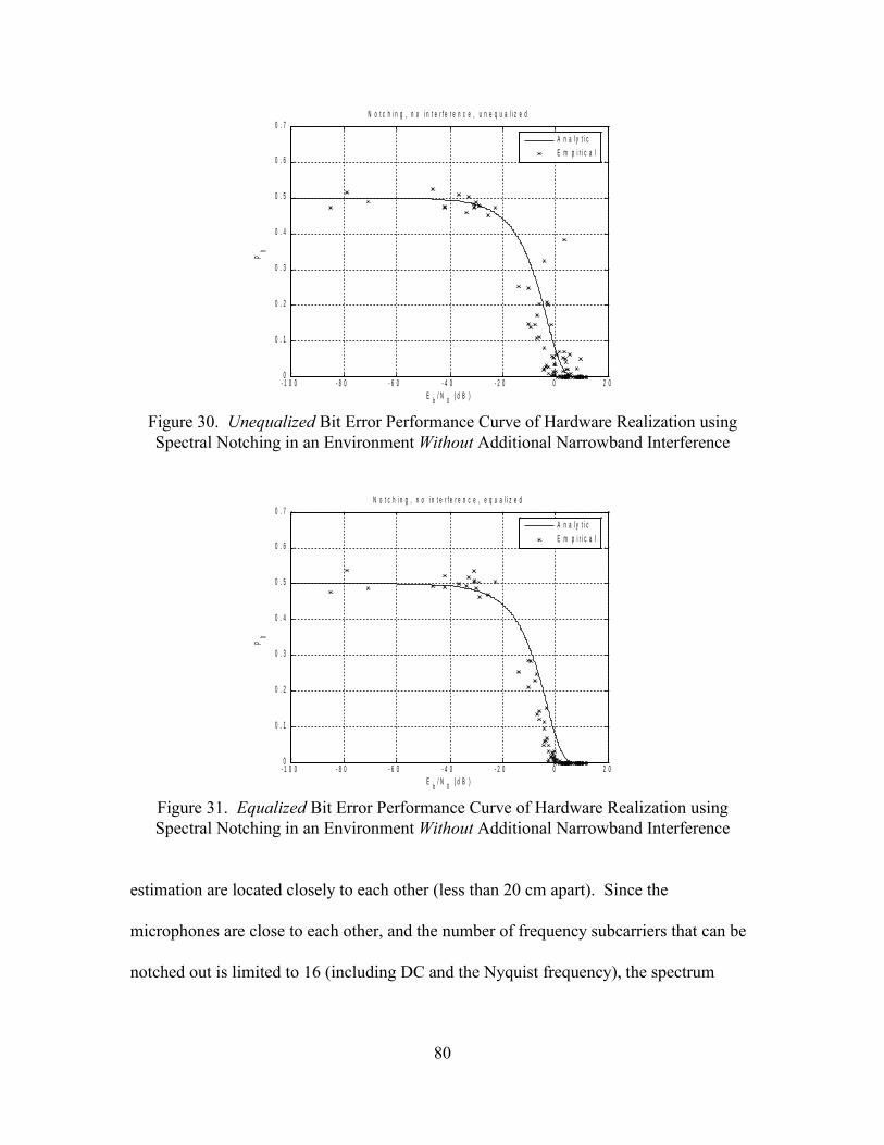
- 1 0 0 - 8 0 - 6 0 - 4 0 - 2 0 0 2 00
0 . 1
0 . 2
0 . 3
0 . 4
0 . 5
0 . 6
0 . 7
Eb
/ N0
( d B )
Pb
N o t c h i n g , n o i n t e r f e r e n c e , u n e q u a l i z e d
A n a l y t i c
E m p i r i c a l
Figure 30. Unequalized Bit Error Performance Curve of Hardware Realization using Spectral Notching in an Environment Without Additional Narrowband Interference
- 1 0 0 - 8 0 - 6 0 - 4 0 - 2 0 0 2 00
0 . 1
0 . 2
0 . 3
0 . 4
0 . 5
0 . 6
0 . 7
Eb
/ N0
( d B )
Pb
N o t c h i n g , n o i n t e r f e r e n c e , e q u a l i z e d
A n a l y t i c
E m p i r i c a l
Figure 31. Equalized Bit Error Performance Curve of Hardware Realization using Spectral Notching in an Environment Without Additional Narrowband Interference
estimation are located closely to each other (less than 20 cm apart). Since the
microphones are close to each other, and the number of frequency subcarriers that can be
notched out is limited to 16 (including DC and the Nyquist frequency), the spectrum
80
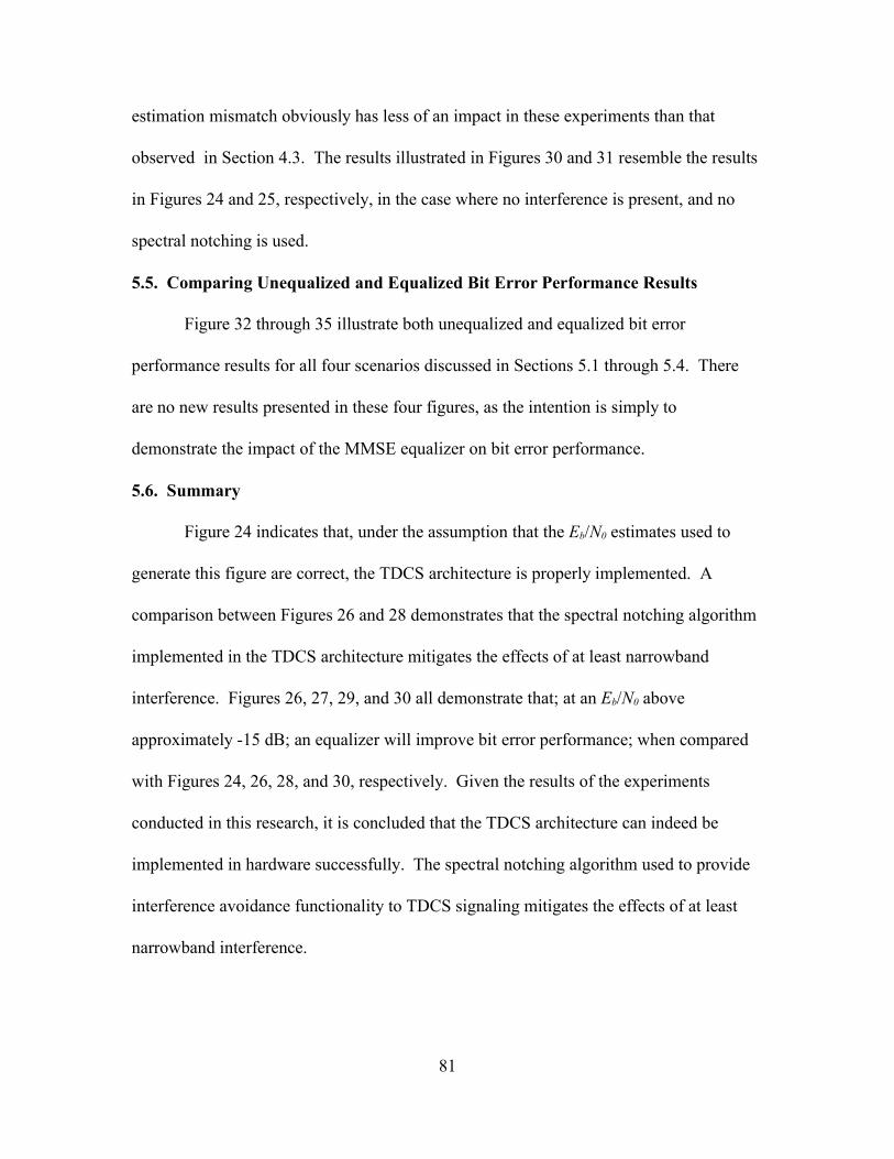
estimation mismatch obviously has less of an impact in these experiments than that
observed in Section 4.3. The results illustrated in Figures 30 and 31 resemble the results
in Figures 24 and 25, respectively, in the case where no interference is present, and no
spectral notching is used.
5.5. Comparing Unequalized and Equalized Bit Error Performance Results
Figure 32 through 35 illustrate both unequalized and equalized bit error
performance results for all four scenarios discussed in Sections 5.1 through 5.4. There
are no new results presented in these four figures, as the intention is simply to
demonstrate the impact of the MMSE equalizer on bit error performance.
5.6. Summary
Figure 24 indicates that, under the assumption that the Eb/N0 estimates used to
generate this figure are correct, the TDCS architecture is properly implemented. A
comparison between Figures 26 and 28 demonstrates that the spectral notching algorithm
implemented in the TDCS architecture mitigates the effects of at least narrowband
interference. Figures 26, 27, 29, and 30 all demonstrate that; at an Eb/N0 above
approximately -15 dB; an equalizer will improve bit error performance; when compared
with Figures 24, 26, 28, and 30, respectively. Given the results of the experiments
conducted in this research, it is concluded that the TDCS architecture can indeed be
implemented in hardware successfully. The spectral notching algorithm used to provide
interference avoidance functionality to TDCS signaling mitigates the effects of at least
narrowband interference.
81

- 1 0 0 - 8 0 - 6 0 - 4 0 - 2 0 0 2 00
0 . 1
0 . 2
0 . 3
0 . 4
0 . 5
0 . 6
0 . 7
Eb
/ N0
( d B )
Pb
N o n o t c h i n g , n o i n t e r f e r e n c e
A n a l y t i c
E m p i r i c a l u n e q u a l i z e dE m p i r i c a l e q u a l i z e d
Figure 32. Comparison of Unequalized and Equalized Bit Error Performance in Scenario with No Spectral Notching and No Narrowband Interference Added to the Environment
- 1 0 0 - 8 0 - 6 0 - 4 0 - 2 0 0 2 00
0 . 1
0 . 2
0 . 3
0 . 4
0 . 5
0 . 6
0 . 7
Eb
/ N0
( d B )
Pb
N o n o t c h i n g , i n t e r f e r e n c e p r e s e n t
A n a l y t i c
E m p i r i c a l u n e q u a l i z e dE m p i r i c a l e q u a l i z e d
Figure 33. Comparison of Unequalized and Equalized Bit Error Performance in Scenario with No Spectral Notching and with Additional Narrowband Interference
82

- 1 0 0 - 8 0 - 6 0 - 4 0 - 2 0 0 2 00
0 . 1
0 . 2
0 . 3
0 . 4
0 . 5
0 . 6
0 . 7
Eb
/ N0
( d B )
Pb
N o t c h i n g , i n t e r f e r e n c e p r e s e n t
A n a l y t i c
E m p i r i c a l u n e q u a l i z e dE m p i r i c a l e q u a l i z e d
Figure 34. Comparison of Unequalized and Equalized Bit Error Performance in Scenario with Spectral Notching and with Additional Narrowband Interference
- 1 0 0 - 8 0 - 6 0 - 4 0 - 2 0 0 2 00
0 . 1
0 . 2
0 . 3
0 . 4
0 . 5
0 . 6
0 . 7
Eb
/ N0
( d B )
Pb
N o t c h i n g , n o i n t e r f e r e n c e
A n a l y t i c
E m p i r i c a l u n e q u a l i z e dE m p i r i c a l e q u a l i z e d
Figure 35. Comparison of Unequalized and Equalized Bit Error Performance in Scenario with Spectral Notching and No Narrowband Interference Added to the Environment
83

VI. Conclusion
Given experimental results obtained in this research, it is concluded that the
TDCS architecture can indeed be implemented successfully in hardware. The spectral
notching algorithm, as used to provide interference avoidance functionality to TDCS
signaling, effectively mitigates the effects of narrowband interference (the only
interference considered for this work).
There were three objectives for this research effort. The first of these objectives,
to compare the bit error performance of a TDCS hardware implementation with simulated
results from literature, has been met. This comparison has been completed, and results
provided in Chapter V validate the simulated results from literature. The second goal,
assessing the capability of a DSP in hosting TDCS transmit/receive functionality, has
been met. The DSK used for transmission and reception is indeed capable of hosting the
TDCS design. The third goal, examining the utility of applying a method of waveform
sculpting other than spectral notching, has been met. This comparison has been
completed and results presented in Chapter IV suggest that spectral notching may be as
effective as water-filling in providing interference avoidance functionality. Furthermore,
spectral notching does not require the computational overhead of water-filling. This
result appears to validate incorporation of the SMSE frequency “use” vector, as expressed
in (15), to mitigate interference by assigning a one or a zero in all elements of the vector.
Collectively, the goals of this research have been successfully met; the TDCS concept can
indeed be successfully implemented in hardware. While the system demonstrated under
this research is admittedly a scaled version of what would be fielded for practical
84

applications, none of the results obtained preclude TDCS from future implementation in a
wireless communications link.
6.1. Recommendations for Further Research
Executing this research effort led to the uncovering of several areas where further
study is recommended. These areas are as follows:
1. The implementation of SMSE+ signaling, as discussed by Roberts [11], onboard a
DSP-based hardware platform.
2. The implementation of a wavelet-based spectrum estimation algorithm in
hardware. A WDCS could be implemented as a standalone realization, or
wavelet-domain spectrum estimation could be integrated into SMSE+ signaling
and then implemented.
3. The implementation of a hardware realization in a multiple access network.
4. The use of higher-order PSK constellations when implementing TDCS or SMSE+
in hardware.
5. The implementation of real-time SMSE+ or TDCS processing in hardware, to
include the embedding of acquisition and fast equalizer algorithms.
6. Much of the DSK firmware uses floating-point calculations. These are more
computationally expensive than fixed-point calculations, and are probably
unnecessary. Conversion to fixed-point processing is recommended to better
optimize the cognitive user pair. An example of conversion techniques for use
with trigonometric functions like sine and cosine are described in literature [32],
and are recommended for further study.
85
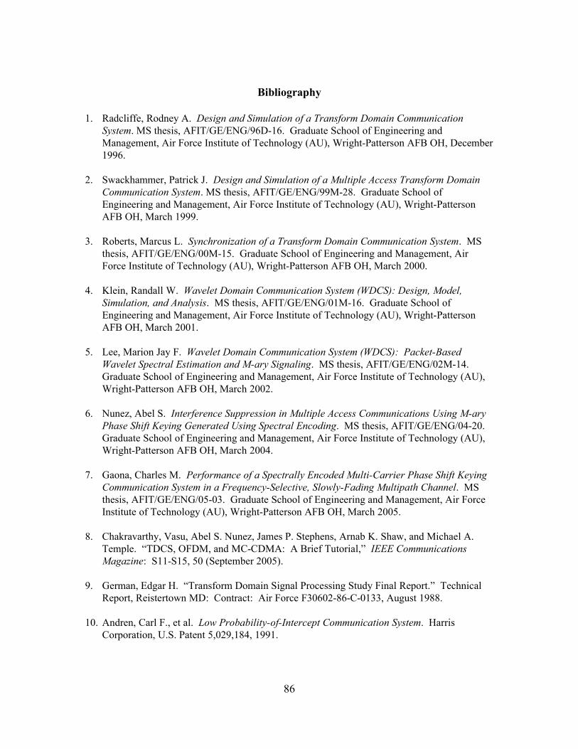
Bibliography
1. Radcliffe, Rodney A. Design and Simulation of a Transform Domain Communication System. MS thesis, AFIT/GE/ENG/96D-16. Graduate School of Engineering and Management, Air Force Institute of Technology (AU), Wright-Patterson AFB OH, December 1996.
2. Swackhammer, Patrick J. Design and Simulation of a Multiple Access Transform Domain Communication System. MS thesis, AFIT/GE/ENG/99M-28. Graduate School of Engineering and Management, Air Force Institute of Technology (AU), Wright-Patterson AFB OH, March 1999.
3. Roberts, Marcus L. Synchronization of a Transform Domain Communication System. MS thesis, AFIT/GE/ENG/00M-15. Graduate School of Engineering and Management, Air Force Institute of Technology (AU), Wright-Patterson AFB OH, March 2000.
4. Klein, Randall W. Wavelet Domain Communication System (WDCS): Design, Model, Simulation, and Analysis. MS thesis, AFIT/GE/ENG/01M-16. Graduate School of Engineering and Management, Air Force Institute of Technology (AU), Wright-Patterson AFB OH, March 2001.
5. Lee, Marion Jay F. Wavelet Domain Communication System (WDCS): Packet-Based Wavelet Spectral Estimation and M-ary Signaling. MS thesis, AFIT/GE/ENG/02M-14. Graduate School of Engineering and Management, Air Force Institute of Technology (AU), Wright-Patterson AFB OH, March 2002.
6. Nunez, Abel S. Interference Suppression in Multiple Access Communications Using M-ary Phase Shift Keying Generated Using Spectral Encoding. MS thesis, AFIT/GE/ENG/04-20. Graduate School of Engineering and Management, Air Force Institute of Technology (AU), Wright-Patterson AFB OH, March 2004.
7. Gaona, Charles M. Performance of a Spectrally Encoded Multi-Carrier Phase Shift Keying Communication System in a Frequency-Selective, Slowly-Fading Multipath Channel. MS thesis, AFIT/GE/ENG/05-03. Graduate School of Engineering and Management, Air Force Institute of Technology (AU), Wright-Patterson AFB OH, March 2005.
8. Chakravarthy, Vasu, Abel S. Nunez, James P. Stephens, Arnab K. Shaw, and Michael A. Temple. “TDCS, OFDM, and MC-CDMA: A Brief Tutorial,” IEEE Communications Magazine: S11-S15, 50 (September 2005).
9. German, Edgar H. “Transform Domain Signal Processing Study Final Report.” Technical Report, Reistertown MD: Contract: Air Force F30602-86-C-0133, August 1988.
10. Andren, Carl F., et al. Low Probability-of-Intercept Communication System. Harris Corporation, U.S. Patent 5,029,184, 1991.
86

11. Roberts, Marcus L. A General Framework for Analyzing, Characterizing, and Implementing Spectrally Modulated, Spectrally Encoded Signals. Air Force Institute of Technology (AU), Wright-Patterson AFB OH, August 2006.
12. Horn, Roger A. and Charles R. Johnson. Topics in Matrix Analysis. Cambridge UK: Cambridge, 1991.
13. Stoica, Petre and Randolph Moses. Spectral Analysis of Signals. Upper Saddle River NJ: Pearson Prentice Hall, 2005.
14. Moses, Randolph. Matlab® functions bartlettse.m, welchse.m, and periodogramse.m. Matlab® function software. http://www.ece.osu.edu/~randy/SAtext/sm-Matlab®-2ed.zip. 29 January 2007.
15. Moses, Randolph. “Lecture notes to accompany Introduction to Spectral Analysis.” Presentation slideshow. http://www.ece.osu.edu/~randy/SAtext/sm-slides-2ed-ver0.9.pdf. 29 January 2007.
16. Proakis, John G. and Masoud Salehi. Communications Systems Engineering, Second Edition. Upper Saddle River NJ: Prentice Pearson Hall, 2002.
17. Dinur, Nati and Dov Wulich. “Peak-to-Average Power Ratio in High-Order OFDM,” IEEE Transactions on Communications, Volume 49, Number 6: 1063-1072 (June 2001).
18. Oppenheim, Alan V. and Ronald W. Schafer. Discrete-Time Signal Processing, Second Edition. Upper Saddle River NJ: Prentice Hall, 1999.
19. Sklar, Bernard. Digital Communications: Fundamentals and Applications, Second Edition. Upper Saddle River NJ: Prentice Hall PTR, 2001.
20. Strang, Gilbert. Linear Algebra and Its Applications, Fourth Edition. Belmont CA: Thomson Brooks/Cole, 2006.
21. Mitola, Joseph. Cognitive Radio: An Integrated Agent Architecture for Software Defined Radio. PhD thesis. Royal Institute of Technology, 2000.
22. Popescu, Dimitrie and Christopher Rose. Interference Avoidance Methods for Wireless Systems. New York: Kluwer Academic/Plenum Publishers, 2004.
23. Popescu, Dimitrie, Otilia Popescu and Christopher Rose. “Interference Avoidance Versus Iterative Water Filling in Multiaccess Vector Channels,” Proceedings of the IEEE 60th Vehicular Technologies Conference. 2058-2062, September 2004.
24. Clemens, Neville and Christopher Rose. “Evolving Strategies for Contentious but Efficient Coexistence in Unlicensed Bands.” Presentation slideshow. http://www.winlab.rutgers.edu/~crose/papers/nev_iab3.ppt. 29 January 2007.
87

25. Cover, Thomas M. and Joy A. Thomas. Elements of Information Theory. New York: Wiley-Interscience, 1991.
26. Cass, Stephen. “Hardware for Your Software Radio,” IEEE Spectrum: 52-54 (October 2006).
27. Chassaing, Rulph. Digital Signal Processing and Applications with the C6713 and C6416 DSK. New York: Wiley-Interscience, 2005.
28. TLV320AIC23 Stereo Audio Codec, 8- to 96- kHz, with Integrated Headphone Amplifier Data Manual. Dallas: Texas Instruments, 2001.
29. Press, William H., Brian P. Flannery, Saul A. Teukolsky, and William T. Vetterling. Numerical Recipes in C. Cambridge UK: Cambridge, 1988.
30. Golub, Gene H. and Charles F. Van Loan. Matrix Computations, Third Edition. Baltimore: Johns Hopkins University Press, 1996.
31. Leon-Garcia, Alberto. Probability and Random Processes for Electrical Engineering, Second Edition. Reading MA: Addison Wesley Longman, 1994.
32. Ylöstalo, Jyri. “Function Approximation using Polynomials,” IEEE Signal Processing Magazine, Volume 23, Number 5: 99-102 (September 2006).
88

Vita
Captain Marshall E. Haker graduated from Washingon High School in Vinton, Iowa in 1993. He
enlisted in the United States Air Force soon after graduation from high school, and served as an electronic
signals intelligence analyst at the National Air and Space Intelligence Center (NASIC) at Wright-Patterson
AFB, Ohio. While assigned to NASIC, he was deployed to Saudi Arabia in 1997 in support of Operation
SOUTHERN WATCH and to Europe in 1999 in support of Operation ALLIED FORCE.
After being named to an education and commissioning program in 1999, he pursued undergraduate
studies at The Ohio State University in Columbus, Ohio where he graduated with honors with a Bachelor of
Science in Electrical and Computer Engineering in August 2002. He was subsequently commissioned
through the USAF Officer Training School at Maxwell AFB, Alabama in December 2002.
His first assignment upon commissioning was to the Oklahoma City Air Logistics Center
(OC-ALC) at Tinker AFB, Oklahoma. More specifically, he served in the 827th Aircraft Sustainment
Group as an electrical systems engineer, where he led the engineering effort on multiple communications
and situational awareness avionics upgrade and sustainment efforts onboard the KC-135 airborne refueler.
In April 2004, he was moved within OC-ALC to the 76th Commodities Maintenance Group where he
served as the lead electrical engineer tasked with the sustainment and upgrading of the B-52, C/KC-135,
and E-3 radome electrical test range at Tinker AFB. The success of the four person engineering team
charged with ensuring the continued operation of the test range, an effort in which he personally designed
the modernized radio frequency signal processing architecture, led to the team being awarded the 2006 U.S.
Air Force Chief of Staff Team Excellence Award.
In August 2005, he entered the Graduate School of Engineering and Management, Air Force
Institute of Technology (AFIT). Upon completion of his Masters Degree at AFIT, Captain Haker will be
assigned to the Air Force Research Laboratory Sensors Directorate, where he will continue his research into
cognitive and software-defined wireless communications and non-communications methods.
89

REPORT DOCUMENTATION PAGEForm ApprovedOMB No. 074-0188
The public reporting burden for this collection of information is estimated to average 1 hour per response, including the time for reviewing instructions, searching existing data sources, gathering and maintaining the data needed, and completing and reviewing the collection of information. Send comments regarding this burden estimate or any other aspect of the collection of information, including suggestions for reducing this burden to Department of Defense, Washington Headquarters Services, Directorate for Information Operations and Reports (0704-0188), 1215 Jefferson Davis Highway, Suite 1204, Arlington, VA 22202-4302. Respondents should be aware that notwithstanding any other provision of law, no person shall be subject to an penalty for failing to comply with a collection of information if it does not display a currently valid OMB control number. PLEASE DO NOT RETURN YOUR FORM TO THE ABOVE ADDRESS.1. REPORT DATE (DD-MM-YYYY)22-03-2007
2. REPORT TYPE Master’s Thesis
3. DATES COVERED (From – To)Jan 2006 – Mar 2007
4. TITLE AND SUBTITLE
Hardware Realization of a Transform Domain Communication System
5a. CONTRACT NUMBER
5b. GRANT NUMBER
5c. PROGRAM ELEMENT NUMBER
6. AUTHOR(S)
Haker, Marshall, E., Captain, USAF
5d. PROJECT NUMBER
5e. TASK NUMBER
5f. WORK UNIT NUMBER
7. PERFORMING ORGANIZATION NAMES(S) AND ADDRESS(S) Air Force Institute of Technology Graduate School of Engineering and Management (AFIT/EN)
2950 Hobson Way WPAFB OH 45433-7765
8. PERFORMING ORGANIZATION REPORT NUMBER
AFIT/GE/ENG/07-10
9. SPONSORING/MONITORING AGENCY NAME(S) AND ADDRESS(ES) AFRL/SNRW
Attn: Mr. Vasu Chakravarthy 2241 Avionics Circle WPAFB OH 45433 DSN: 785-5579x4245
10. SPONSOR/MONITOR’S ACRONYM(S)
11. SPONSOR/MONITOR’S REPORT NUMBER(S)
12. DISTRIBUTION/AVAILABILITY STATEMENT APPROVED FOR PUBLIC RELEASE; DISTRIBUTION UNLIMITED.
13. SUPPLEMENTARY NOTES
14. ABSTRACT The purpose of this research was to implement a Transform Domain Communication System (TDCS) in hardware and compare experimental bit error performance with results published in literature. The intent is to demonstrate the effectiveness or ineffectiveness of a TDCS in communicating binary data across a real channel. In this case, an acoustic channel that is laden with narrowband interference was considered. A TDCS user pair was constructed to validate the proposed design using Matlab® to control a PC sound card. The proposed TDCS design used the Bartlett method of spectrum estimation, the spectral notching algorithm found in TDCS literature, quadrature phase shift keying, and minimum mean square error transverse equalization to mitigate the effects of noise and intersymbol interference. Water-filling was evaluated as an alternative to spectral notching for performing waveform design and is shown to perform equivalently. Validated software was migrated to code suitable for use onboard a Digital Signal Processor Starter Kit (DSK). Two DSK boards were used, one for transmission and reception, and bit error performance results were obtained. Bit error analysis reveals that the TDCS hardware performs approximately the same as literature suggests.
15. SUBJECT TERMSTransform Domain Communication System, Digital Communications, Adaptive Communications, Secure Communications, Radio Interference
16. SECURITY CLASSIFICATION OF: REPORTU
ABSTRACTU
c. THIS PAGEU
17. LIMITATION OF ABSTRACT
UU
18. NUMBER OF PAGES102
19a. NAME OF RESPONSIBLE PERSONRichard K. Martin (ENG)
19b. TELEPHONE NUMBER (Include area code)(937) 255-3636, ext 4625; e-mail: [email protected]
Standard Form 298 (Rev: 8-98)Prescribed by ANSI Std. Z39-18
90